J Geod (2010) 84:605–624 DOI 10.1007/s00190-010-0401-7 ORIGINAL ARTICLE The celestial mechanics approach: theoretical foundations Gerhard Beutler · Adrian Jäggi · Leoš Mervart · Ulrich Meyer Received: 31 October 2009 / Accepted: 29 July 2010 / Published online: 24 August 2010 © Springer-Verlag 2010 Abstract Gravity field determination using the measure- ments of Global Positioning receivers onboard low Earth orbiters and inter-satellite measurements in a constellation of satellites is a generalized orbit determination problem involv- ing all satellites of the constellation. The celestial mechanics approach (CMA) is comprehensive in the sense that it encom- passes many different methods currently in use, in particular so-called short-arc methods, reduced-dynamic methods, and pure dynamic methods. The method is very flexible because the actual solution type may be selected just prior to the com- bination of the satellite-, arc- and technique-specific normal equation systems. It is thus possible to generate ensembles of substantially different solutions—essentially at the cost of generating one particular solution. The article outlines the general aspects of orbit and gravity field determination. Then the focus is put on the particularities of the CMA, in partic- ular on the way to use accelerometer data and the statistical information associated with it. Keywords Celestial mechanics · Orbit determination · Global gravity field modeling · CHAMP · GRACE 1 Problem description and overview This article has the focus on the theoretical foundations of the so-called celestial mechanics approach (CMA). Applications G. Beutler (B ) · A. Jäggi · U. Meyer Astronomical Institute, University of Bern, Sidlerstrasse 5, 3012 Bern, Switzerland e-mail: [email protected] L. Mervart Institute of Advanced Geodesy, Czech Technical University, K-152, FSvCVVT, Thakurova 7, 16629 Prague 6-Dejvice, Czech Republic of the CMA, in particular to the GRACE mission, may be found in Beutler et al. (2010) and Jäggi et al. (2010b). The determination of the Earth’s global gravity field using the data of space missions is nowadays either based on 1. the observations of spaceborne Global Positioning (GPS) receivers onboard low Earth orbiters (LEOs) (see Reigber et al. 2004), 2. or precise inter-satellite distance monitoring of a close satellite constellation using microwave links (combined with the measurements of the GPS receivers on all space- crafts involved) (see Tapley et al. 2004), 3. or on gradiometer measurements realized by three pairs of three-dimensional accelerometers onboard a LEO measuring the complete gravitational tensor of the Earth along the satellite’s trajectory (combined with the obser- vations of the onboard GPS receiver) (see Drinkwater et al. 2006). The CHAllenging Minisatellite Payload (CHAMP) mission is generating the first kind of data set, the Gravity Recov- ery And Climate Experiment (GRACE) mission the second one, and the Gravity field and steady-state Ocean Circulation Explorer (GOCE) mission the third one. The first type of data is available for all three missions. The gravity fields emerging from one of the above data sets are often combined in a statistically correct way with the solutions obtained from Satellite Laser Ranging (SLR) and/or from ground-based or airborne gravimetry (see Förste et al. 2008). We do not consider combinations of this kind here, but focus on the contribution of the mentioned satellite missions. The above observational data are supported by the mea- surements of accelerometers (Touboul et al. 1999), e.g., placed in the satellite’s center of mass, which give—as a 123 brought to you by CORE View metadata, citation and similar papers at core.ac.uk provided by RERO DOC Digital Library

Welcome message from author
This document is posted to help you gain knowledge. Please leave a comment to let me know what you think about it! Share it to your friends and learn new things together.
Transcript

J Geod (2010) 84:605–624DOI 10.1007/s00190-010-0401-7
ORIGINAL ARTICLE
The celestial mechanics approach: theoretical foundations
Gerhard Beutler · Adrian Jäggi · Leoš Mervart ·Ulrich Meyer
Received: 31 October 2009 / Accepted: 29 July 2010 / Published online: 24 August 2010© Springer-Verlag 2010
Abstract Gravity field determination using the measure-ments of Global Positioning receivers onboard low Earthorbiters and inter-satellite measurements in a constellation ofsatellites is a generalized orbit determination problem involv-ing all satellites of the constellation. The celestial mechanicsapproach (CMA) is comprehensive in the sense that it encom-passes many different methods currently in use, in particularso-called short-arc methods, reduced-dynamic methods, andpure dynamic methods. The method is very flexible becausethe actual solution type may be selected just prior to the com-bination of the satellite-, arc- and technique-specific normalequation systems. It is thus possible to generate ensemblesof substantially different solutions—essentially at the costof generating one particular solution. The article outlines thegeneral aspects of orbit and gravity field determination. Thenthe focus is put on the particularities of the CMA, in partic-ular on the way to use accelerometer data and the statisticalinformation associated with it.
Keywords Celestial mechanics · Orbit determination ·Global gravity field modeling · CHAMP · GRACE
1 Problem description and overview
This article has the focus on the theoretical foundations of theso-called celestial mechanics approach (CMA). Applications
G. Beutler (B) · A. Jäggi · U. MeyerAstronomical Institute, University of Bern, Sidlerstrasse 5,3012 Bern, Switzerlande-mail: [email protected]
L. MervartInstitute of Advanced Geodesy, Czech Technical University,K-152, FSvCVVT, Thakurova 7, 16629 Prague 6-Dejvice,Czech Republic
of the CMA, in particular to the GRACE mission, may befound in Beutler et al. (2010) and Jäggi et al. (2010b).
The determination of the Earth’s global gravity field usingthe data of space missions is nowadays either based on
1. the observations of spaceborne Global Positioning (GPS)receivers onboard low Earth orbiters (LEOs) (seeReigber et al. 2004),
2. or precise inter-satellite distance monitoring of a closesatellite constellation using microwave links (combinedwith the measurements of the GPS receivers on all space-crafts involved) (see Tapley et al. 2004),
3. or on gradiometer measurements realized by three pairsof three-dimensional accelerometers onboard a LEOmeasuring the complete gravitational tensor of the Earthalong the satellite’s trajectory (combined with the obser-vations of the onboard GPS receiver) (see Drinkwateret al. 2006).
The CHAllenging Minisatellite Payload (CHAMP) missionis generating the first kind of data set, the Gravity Recov-ery And Climate Experiment (GRACE) mission the secondone, and the Gravity field and steady-state Ocean CirculationExplorer (GOCE) mission the third one. The first type of datais available for all three missions.
The gravity fields emerging from one of the above datasets are often combined in a statistically correct way withthe solutions obtained from Satellite Laser Ranging (SLR)and/or from ground-based or airborne gravimetry (see Försteet al. 2008). We do not consider combinations of this kindhere, but focus on the contribution of the mentioned satellitemissions.
The above observational data are supported by the mea-surements of accelerometers (Touboul et al. 1999), e.g.,placed in the satellite’s center of mass, which give—as a
123
brought to you by COREView metadata, citation and similar papers at core.ac.uk
provided by RERO DOC Digital Library

606 G. Beutler et al.
function of time—biased and scaled values of the non-gravitational accelerations acting on the satellites. Themeasurements are performed in three orthogonal directions,usually closely related to the radial (R), the out-of-plane (W ),and the along-track component (S), which are associatedwith the unit vectors er in the radial, eW in the out-of-plane,and eS
.= eW × eR in the (approximate) along-track direc-tions. Accelerometer bias parameters have to be set up andestimated in the generalized orbit estimation process. Oneshould also solve for accelerometer scale parameters. Theseparameters are, however, highly correlated with the once-per-revolution dynamic parameters, which is why we usu-ally do not solve for them. In order to refer the GPS- andinter-satellite measurements to the satellites’ centers of mass,the attitude of the satellite-fixed coordinate system has to beoriented in the inertial system (using star-tracking cameras)and the sensor offsets in the satellite-fixed coordinate systemhave to be known.
The complexity of the parameter estimation problem maybe considerably reduced by not analyzing the original (phaseand code) GPS measurements in the gravity field estimationprocess, but rather the LEOs’ so-called kinematic positions(Švehla et al. 2004), using optionally parts of the variance–covariance matrices, hereafter called simply covariancematrices, associated with them. As the GPS-derived kine-matic positions are not original measurements, but usedsubsequently as observations in the parameter estimationprocedures, we also refer to them as pseudo-observationsor pseudo-measurements. Kinematic LEO orbits are derivedfrom the LEO receivers’ GPS code and phase measurementsusing a precise point positioning (PPP) procedure (Zumbergeet al. 1997). More information is provided in Sect. 3.2.
Static “satellite-only” gravity fields based on long dataspans should be based on solutions not making use of infor-mation other than that contained in the measurements. Com-binations with other solutions on the normal equation system(NEQ) level involving other techniques should be made afterthe satellite-only solutions. This demand is “rather absolute”and never can be really met, because one will, e.g., alwaysmake use (and be it only for reasons of computation effi-ciency) of a rather good a priori gravity field—meaning thatreasonable approximate values are used at least for the termsup to degree n = 20. The dependency on the a priori gravityfield was studied in some detail in Jäggi et al. (2010b), wherethe EGM96 (Lemoine et al. 1997) served as a priori field.Virtually the same results were obtained when using a muchbetter a priori field. We are therefore confident that the CMAmeets the demand of “independency on the a priori gravityfield” to a great extent. As long as all coefficients set up inthe a priori field are also estimated in the subsequent param-eter estimation procedure, the impact of the a priori gravityfield on the estimated field must be small—and should disap-pear completely, if the solution is iteratively improved using
the estimated parameters as new a priori values in a seconditeration step. The dependency on many other backgroundmodels (e.g., tides) are much more problematic and difficultto avoid.
The situation is different if the interest is on the time vary-ing part of the gravity field using a rather short data span(usually one month in the case of GRACE). There it maymake sense to generate solutions, which are based on an apriori gravity field of high degree and order (e.g., with a cut-off degree of n = 150–180, which was derived previously),and to determine the gravity field parameters up to a modestlimiting degree only, e.g., between 20 and 60. The aspect ofextracting the time varying part of the gravity field is, how-ever, not in the center of this article. Such a set-up to studythe impact of different solution strategies on the achievableresults is used in Beutler et al. (2010). Note, as well, that sev-eral research centers determine monthly gravity fields fromGRACE up to degree 120 and that Liu et al. (2010) retrievedtemporal signals above degree 70 in monthly GRACE gravityfields using filtering techniques.
The CMA has its roots in the Bernese GPS Software (Dachet al. 2007), which was extensively used for determining theorbits of Global Navigation Satellite Systems (GNSS). TheCMA was generalized to determine the orbits of LEOs byJäggi (2007) with special emphasis on the stochastic proper-ties of the orbits. In recent years the CMA was further devel-oped and used for gravity field determination. This articlerepresents the first consistent description of the CMA, thekey aspects of which are:
− The CMA is based on the foundations of celestialmechanics. It is a package designed for orbit and for grav-ity field determination, where the latter task is merely ageneralization of the former.
− The modularity of the CMA allows it to study or improveindividual contributions to a resulting orbit or gravityfield. It also may be used as an ideal tool for planningfuture space missions (gravity field oriented or other).
− The use of kinematic positions derived from GPS,together with the options to use either the full or onlythe epoch-specific covariance matrices from PPP, is per-fectly suited to study the quality of GPS-only orbits andtheir contribution to gravity fields.
− The CMA is based not on stochastic, but on piecewisedeterministic equations of motion. With its capabilities toset up pseudo-stochastic parameters (of different kinds)with a dense spacing, the CMA orbits may be made closerelatives of solutions of stochastic differential equations.
The aspects of Celestial Mechanics relevant for gravity fielddetermination are described in Sect. 2. The CMA’s responseto these challenges may be found in Sect. 3. Section 4 reviewsdifferent methods used for gravity field determination and
123

The celestial mechanics approach: theoretical foundations 607
puts them in relation to the CMA. Section 5 summarizes themain findings and the conclusions emerging from this work.
2 Orbit and gravity field determination
Every procedure to determine the Earth’s gravity field usingspace data has to be based on the foundations of celestialmechanics. A static gravity field to be derived from the GOCEmission seems to be an exception at first sight, because thekey instrument, the gradiometer, provides the gravitationaltensor along the satellite’s trajectories as in situ measure-ments, which depend only weakly on the satellite’s orbitalmotion. Due to the limited bandwidth of the gradiometer,however, the lower degree harmonics are almost uniquelydetermined by the orbital motion of the GOCE satellite (Pailet al. 2006). Because of the low altitude of the satellite, thegravity field derived from the GOCE GPS data alone shouldalready be of remarkable quality and resolution—and it hasto be combined in a consistent way with the results emergingfrom the gradiometer.
Our procedure should be called more precisely “themethod to generate ensembles of orbits and gravity field solu-tions fully exploiting the degrees of freedom offered by celes-tial mechanics and using the power of applied mathematicsto generate the precise solutions in an efficient way”. As thisdescription is of the lengthy kind, we stick to the short title“CMA”.
Before highlighting the essential elements of our methodin Sect. 3 we review the key characteristics of orbital motionand of gravity field determination in general in this section.
2.1 Equations of motion and their solution
The geocentric position vector r(t) of a satellite’s centerof mass solves the so-called equations of motion for eachtime argument t . These are usually written as second order,non-linear ordinary differential equations based on Newton’sprinciples and on his law of universal gravitation, amended bycorrections due to the special and general theories of relativ-ity. The equations used today are often referred to as param-eterized post-Newtonian equations (Seidelmann 1992). Thesatellite’s position vector r(t) at any given epoch t is a partic-ular solution of the equations of motion defined by the initialposition and velocity vectors r0
.= r(t0) and v0.= r(t0) at an
initial epoch t0. The initial position and velocity vectors arealso referred to as “initial state vector” (with six elements).The initial state vector is defined by six quantities, e.g., theinitial osculating orbital elements. For a general discussionof the orbit determination problem see Beutler (2005, Vol. 1,Chapter 8).
In order to solve the parameter estimation problem, therelationship between the observables (see Sect. 2.2) and the
parameters has to be linearized. Linearization implies forour problems that each orbit (arc) involved is approximatedas a linear function of its defining parameters including thosedynamical parameters common to several or all orbits. In ageneric way a linearized orbit may be written as
r(t) .= r0(t) +npar∑
i=1
∂r0(t)
∂pi(pi − p0i ), (1)
where the a priori orbit (or “initial orbit” or “reference orbit”)r0(t)
.= r(t; p01, p02, . . . , p0,npar ) is a function of time andcharacterized by known approximate values p0i of the param-eters pi , i = 1, 2, . . . , npar; the partial derivatives on therighthand side should be understood as the partial deriva-tives of the function r(t; p1, p2, . . . , pnpar ) w.r.t. the param-eters pi , evaluated at pi = p0i ; npar is the number of orbitparameters defining the orbit r(t). Whereas all methods arebased on a linearized representation of the unknown orbits asa function of the parameters, one should clearly specify howthe reference orbits and the partial derivatives of the referenceorbits w.r.t. the parameters of different type are generated.
2.2 Observables and observations
Two classes of observations (measurements) should be dis-tinguished in modern gravity field determination:
− Class I: observations measuring functions of the satel-lites’ position and/or velocity vectors at particularepochs,
− Class II: observations measuring (parts of) the force field(or functions of the field) acting on the satellites at par-ticular epochs.
The observed functions of the parameters are also referred toas observables.
Kinematic positions derived from spaceborne GPS receiv-ers and the K-Band range or range-rate Level 1b measure-ments of the GRACE mission are typical representatives ofobservations of Class I, accelerometer and gradiometer mea-surements of Class II.
The observations actually used in the parameter adjust-ment process may be the original measurements gained bythe satellites’ sensors or functions thereof. Often it is assumedthat the errors in the original measurements (e.g., the GPSphase or the K-Band Level 1a range measurements) haveparticularly simple statistical characteristics, e.g., indepen-dent and normally distributed. It does not matter whether theoriginal measurements or functions thereof are analyzed inthe adjustment process—as long as the mathematical corre-lations between the errors in the original measurements andthose analyzed are taken into account. If, e.g., the full covari-ance matrix of the kinematic positions covering the entire
123

608 G. Beutler et al.
time span of data as a function of the GPS phase (and code)observations is available and used in the adjustment process(what is, however, usually not done), the results are the sameas if the orbits and/or the gravity fields would have beenestimated directly with the original observations. The sameremarks apply to the use of Level 1b ranges or range-ratesinstead of the Level 1a ranges.
In the absence of Class II observations parameter estima-tion is a straightforward affair. The observations are eitherindependent with known variances or they are linear combi-nations of the original observations of Class I. In the formercase the weight matrix is diagonal, in the latter case fullypopulated. The impact of the non-modeled parts of the forcefield are treated as stochastic quantities by the adjustmentprocess, reflected by an enlarged root mean square (RMS)error a posteriori (w.r.t. the known RMS error a priori) ofthe Class I observations. Pure dynamic methods are usuallybased on this procedure.
Properly taking into account the stochastic properties ofClass II observations is in practice less trivial, because theobservables of Class I are functions of the force field, aswell, i.e., also of the observations of Class II. It is, however,in principle easy to set up a correct analysis involving bothclasses of observations:
1. The observations of the force field have to be introducedwith their known statistical properties into the adjust-ment process, i.e., in addition to the Class I observationequations there is also one observation equation for eachmeasurement of Class II.
2. The impact of the observables of Class II on the obser-vations of Class I has to be taken into account.
Let us outline the correct procedure using the Level 1a accel-erometer observations a′
k of the GRACE mission as an exam-ple. We assume that these measurements are independentand of the same accuracy. In practice, the measurementsa′
k are filtered, resulting in a smoothed series ak0, which isthen used as the empirically given non-gravitational forcein the integration process. In order to analyze the structureof the problem we skip the filtering process and assume thatthe empirical non-gravitational forces are constant in the timeintervals [tk, tk+1] and directly given by the Level 1a data
ak0.= a′
k, t ∈ [tk, tk+1], k = 1, 2, . . . . (2)
This view is statistically correct, because the use of the unfil-tered data is equivalent to the use of the filtered data togetherwith the corresponding correct correlation matrix.
In order to take the statistical nature of the measurementsa′
k into account one must introduce the parameters �ak ,standing for the difference between the true and the mea-sured acceleration. The measurements thus may be writtenas a′
k.= ak0−�ak . The quantities �ak are normal parameters
of the adjustment process governed by the observation equa-tion
�ak = 0, k = 1, 2, . . . . (3)
Assuming that the measurements a′k are not correlated and
all have the same variance σ 2a , the above measurements are
associated with the weights σ 20 /σ 2
a , where σ0 is the standarddeviation of the weight unit used in the adjustment.
The impact of the parameters �ak on the kinematic posi-tions and inter-satellite distances has to be taken into account,as well. This problem is, in principle, easily solved: thedependency of the orbit on the parameters is described ina generic way by Eq. (1), where the �ak are elements of theparameter list. The position and/or velocity vectors are there-fore also linear functions of the �ak corresponding to epochsprior to the observation epoch. The same linear dependencythus also holds for functions of these vectors.
The partial derivatives w.r.t. the �ak can be calculated,without additional computational burden, as linear combina-tions of the partial derivatives w.r.t. the six parameters defin-ing the initial state vector and the partial derivative w.r.t. aconstant force in the direction considered. As the functionaldependency of the Class I observables on the satellite posi-tions and velocities is known anyway for each time argumentt , it is also straightforward to model the influence of thesenew parameters �ak on the Class I observables like range,range-rate, etc. This completes the correct way of taking thestochastic properties of the accelerometer measurements intoaccount. No problems of principle have been encountered.
The problem with this purist approach resides in the poten-tially huge number of additional parameters associated withit: when using accelerometer data with a 0.1 s spacing, oneends up with 864,000 additional parameters in the dailyNEQs—definitely a hopeless affair. The problem can ofcourse be alleviated by taking into account the correlationsonly over short time periods and by (pre-)eliminating theparameters �ak of the short time intervals. There are waysto do this efficiently.
The effort of taking into account the impact of Class IIon Class I observables becomes irrelevant, if their impacton the Class I observables is much smaller than the ClassI RMS errors. For GRACE-like missions this requirementobviously would have an impact on the stochastic propertiesof the range and of the accelerometer observables.
2.3 An experiment applied to an ideal gravity mission
The following simulation illustrates that the above postulatedindependence is not given for all observables of the GRACEmission: a Keplerian orbit is perturbed by normally distrib-uted, random accelerations a′
R,k, a′S,k, a′
W,k in theR-, S- and W -directions, which are constant in the time inter-vals [tk, tk+1], k = 0, 1, 2, . . . , where tk+1 − tk = �tp =
123

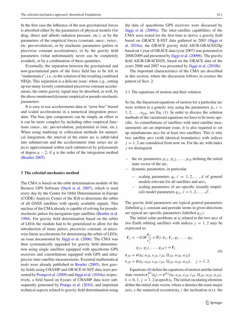
The celestial mechanics approach: theoretical foundations 609
Fig. 1 Residuals in R-, S-,W -directions of an orbitperturbed by piecewise constantaccelerations (spacing of 0.1 s,RMS = 10−10 m/s2) usingvelocities (left) or positions(right) as observations, bothwithout measurement noise
0 50 100 150 200 250 300 350 400−4
−3
−2
−1
0
1
2
3
4 x 10⁻⁹
Time (min)m
/s
radialalong−trackout of plane
0 50 100 150 200 250 300 350 400−2
−1.5
−1
−0.5
0
0.5
1
1.5
2 x 10⁻⁶
Time (min)
m
radialalong−trackout of plane
0.1 s. An RMS error of σa = 10−10 m/s2 is assumed for thesenormally distributed piecewise constant accelerations in thethree directions.
The components of the perturbed position or velocity vec-tor are used as observations (without adding any additionalmeasurement noise) in a conventional least-squares process,which assumes all Class 1 observables as independent and ofthe same accuracy (weight matrix = identity matrix), to esti-mate the orbit of a 6h-arc. The simulation represents a hypo-thetical “super gravity field experiment”, which measureseach component of the two satellites’ position or velocityvectors with infinite accuracy. Its only “weakness” residesin the limited accuracy of the accelerometers. The six ini-tial osculating elements and the unconstrained pulses in theR-, S- and W -directions at 30- min intervals are the param-eters of the orbit determination procedure. Figure 1 (left)shows the residuals of the orbit determination experimentusing the velocity components as observations, and Fig. 1(right) the residuals using the position components. Despitethe fact that the measurement noise of the components of thevelocity and position vectors was assumed to be zero in ourexperiment, the RMS error a posteriori of the orbit determi-nation (based, as mentioned, on a conventional least-squaresestimator) using the components of the velocity vector asobservations is of the order of 10−9 m/s, it is of the order of10−6 m when using the components of the position vector.Whether or not this accelerometer-induced noise on the ClassI observables can be ignored depends on the noise character-istics of the Class I observables.
The results of the simulation experiment may be trans-lated, to some extent, to the realities of the GRACE mission:the GRACE accelerometer measurements—when perform-ing at the promised nominal level—have an impact of thekind illustrated by Fig. 1 on the components of the velocityand the position vector, respectively. These small effects donot matter at all when considering the impact on the GPS-derived positions (we are speaking of position RMS errorsof few centimeters for the kinematic positions).
The accelerometers also have an impact of the orderof magnitude given by Fig. 1 (multiplied by
√2) on the
inter-satellite range-rates and ranges. The RMS errors of theorder of 1–2×10⁻⁷ m/s for inter-satellite range-rates usinga K-Band link (derived by numerical differentiation fromranges) between the satellites is still large compared to theaccelerometer-induced noise in Fig. 1 (left). We thereforeconclude that the impact of the stochastic properties of theGRACE accelerometers on the velocity observable is neg-ligible in terms of the RMS estimated by the least-squaresadjustment—provided the accelerometers perform asclaimed by Touboul et al. (1999). The situation is not soclear for the range observable: Fig. 1 (right) indicates thatsmall accelerometer RMS errors of σa ≈ 10−10 m/s2 gener-ate a systematic pattern in the range residuals of the order of10−6 m. The impact of the accelerometer-induced noise onthe range observable is thus of the same order of magnitudeas the RMS of the Level 1b range measurements and shouldbe captured by methods described in the previous section.
The experiment performed in this section was based, asstated initially, on simplifying assumptions. An in-depth anal-ysis should not be based simply on a comparison of RMSvalues of the involved observations, because of a possibledependency of noise on frequency, but on the power spectraldensities of the range (or range-rate), the accelerometer, andthe GPS-related observables.
2.4 Primary and variational equations
The initial orbit r0(t) in Eq. (1) should be a sufficientlygood approximation of the “final” orbit r(t) (resulting in theparameter estimation process) in order to justify the negli-gence of the non-linear terms.
The initial orbit r0(t) is usually obtained by numericallysolving the equations of motion. The partial derivatives inEq. (1) solve the so-called variational equations (seeSect. 3.7). As the number of parameters is counted in tensof thousands in gravity field determination, it is important tosolve the variational equations efficiently.
In the context of parameter estimation the equations ofmotion are called the primary equations. The primary equa-tions have to be solved as accurately as needed, the actual
123

610 G. Beutler et al.
requirements being dictated by the accuracy of the observa-tions. When analyzing inter-satellite distances accurate to afew microns, “as accurately as needed” translates into “asaccurately as possible” (see also Sect. 3.5).
2.5 Parameter estimation
Gravity field determination only makes sense, if the totalnumber of observations vastly exceeds the total number ofparameters. An estimation principle has to transform theobservation equations into a system of equations, where thedimension equals the number of parameters. The methodof least-squares demands the sum of the weighted residualsquares to be minimum, which in turn implies that the partialderivatives of this sum w.r.t. each parameter are zero. Theleast-squares principle thus leads to a system of linear equa-tions, the NEQs, the dimension of which equals the number ofparameters. For more information concerning least-squaresand other estimation principles we refer to Strang and Borre(1997).
2.6 Arc, arc length
We refer to a satellite arc as the trajectory r(t) between timelimits tb ≤ t ≤ te, represented by one and the same initialposition and velocity vectors r0
.= r(t0) and v0.= r(t0).
The arc length is the length |te − tb| of the time intervalIarc = [tb, te]. Usually this time interval coincides with theinterval containing all observations used to determine the ini-tial state vector and other orbit parameters. t0 usually coin-cides with tb.
The arc length is an important option available to the ana-lyst. In the history of celestial mechanics one usually madethe attempt to render the arcs as long as possible in order tominimize the total number of parameters of a particular task(Biancale et al. 2000). Prior to the satellite missions of thetwenty-first century most classical problems were governedby relatively few observations.
The age of modern gravity field determination has led to arevision of this concept. The availability of virtually continu-ous tracking by GPS (typically allowing for the determinationof a satellite position every 10–30 s) and of continuous inter-satellite measurements made short-arc methods a valuableand attractive alternative absorbing many biases of unclearorigin into the initial state vectors. The success of proce-dures developed by Mayer-Gürr et al. (2005) and Mayer-Gürr(2008) underlines this statement.
2.7 Orbit determination
Orbit determination was originally understood as the task ofdetermining six parameters, defining the initial state vector ofthe satellite, using all observations available in a certain time
interval. A slightly more general case is that of determiningthe initial state vector and a certain number of arc-specificparameters from the mentioned set of observations (see, e.g.,Beutler 2005). In the most general case one has to determinein addition parameters defining the force field. Such parame-ters may be either satellite- and arc-specific or -independent.Parameters of this kind may be called dynamic parameters.As gravity field parameters are dynamic parameters, gravityfield determination is nothing but a generalized orbit deter-mination task.
As the same dynamic parameters may show up in orbitsof different satellites or in different arcs of the same satellite,the generalized orbit determination problem may be morecomplex than the pure orbit determination problem: the arc-specific parameters have to be pre-eliminated from the arc-specific NEQs, these reduced NEQs have to be accumulatedand eventually the dynamic parameters common to all arcsand satellites have to be estimated by solving the resultingNEQ. The arc-specific parameters may then be calculatedin a re-substitution procedure (if sufficient information wasstored in the pre-elimination step) or by a pure orbit deter-mination problem using the previously determined satellite-and arc-independent parameters as known values.
2.8 Empirical and non-gravitational accelerations
From the mathematical point of view empirical dynamicforces are indistinguishable from deterministic forces basedon a physical force model. Empirical dynamic forces usu-ally are meant to absorb poorly modelled parts of the forcefield. Typical empirical forces are constant, or once-, twice-,etc. per-revolution forces in predefined directions (e.g., inR, S, and W ). The independent argument associated withthe periodic forces needs to be specified (e.g., the argumentof latitude u, the osculating true anomaly v, etc.).
Empirical forces are, e.g., required to solve for at leastthree constant accelerations per arc (in the 3 nominallyorthogonal measurement directions), when using three-dimensional accelerometers to define the non-gravitationalforces, because accelerometer measurements are biased.
The separation of the gravitational and the non-gravitational forces is an important issue for gravity fielddetermination. For gravity field determination with theCHAMP, GRACE, and GOCE missions the following casescan be distinguished (where we use the Class I and Class IIobservables as introduced in Sect. 2.2):
1. Use of the Class I observables (e.g., kinematic positionswhen determining the gravity field from GPS only, kine-matic positions and K-Band range-rates or ranges in thecase of the GRACE mission)
2. Use of Class I and of Class II observables (in particularof accelerometer data).
123
The celestial mechanics approach: theoretical foundations 611
In the first case the influence of the non-gravitational forcesis absorbed either by the parameters of physical models (fordrag, direct and albedo radiation pressure, etc.), or by theparameters of the empirical forces (constant, once-, twice-,etc. per-revolution), or by stochastic parameters (pulses orpiecewise constant accelerations), or by the gravity fieldparameters (what unfortunately never can be completelyavoided), or by a combination of these quantities.
Eventually, the separation between the gravitational andnon-gravitational parts of the force field has to be left to“mathematics”, i.e., to the solution of the resulting combinedNEQs. This separation is a delicate issue: when, e.g., settingup too many loosely constrained piecewise constant acceler-ations, the entire gravity signal may be absorbed, as well, bythe above mentioned dynamic empirical or pseudo-stochasticparameters.
It is easy to use accelerometer data as “error free” biasedand scaled accelerations in a numerical integration proce-dure. The bias (per component) can be simply an offset orit can be more complex by including other empirical func-tions (once-, etc. per-revolution, polynomial in time, etc.).When using multistep or collocation methods for numeri-cal integration, the interval of the entire arc is subdividedinto subintervals and the accelerometer time series are defacto approximated within each subinterval by polynomialsof degree q − 2, if q is the order of the integration method(Beutler 2005).
3 The celestial mechanics method
The CMA is based on the orbit determination module of theBernese GPS Software (Dach et al. 2007), which is usedevery day by the Center for Orbit Determination in Europe(CODE) Analysis Center of the IGS to determine the orbitsof all GNSS satellites with openly available signals. Thisnucleus of the CMA already is capable of solving for pseudo-stochastic pulses for navigation-type satellites (Beutler et al.1994). For gravity field determination based on the orbitsof LEOs the module had to be generalized to allow for theintroduction of many pulses, piecewise constant, or piece-wise linear accelerations for determining the orbits of LEOs,an issue documented by Jäggi et al. (2006). The CMA wasthen systematically upgraded for gravity field determina-tion using single satellites equipped with spaceborne GPSreceivers and constellations equipped with GPS and ultra-precise inter-satellite measurements. Essential mathematicaltools were already published in Beutler (2005), first grav-ity fields using CHAMP and GRACE hl-SST data were pre-sented by Prange et al. (2009) and Jäggi et al. (2010a), respec-tively, a field based on 6 years of CHAMP data were sub-sequently generated by Prange et al. (2010), and importanttechnical aspects related to gravity field determination using
the data of spaceborne GPS receivers were discussed byJäggi et al. (2009a). The inter-satellite capabilities of theCMA were tested for the first time to derive a gravity fieldbased on GRACE ll-SST data gathered in 2003 (Jäggi etal. 2010a), the GRACE gravity field AIUB-GRACE02Spbased on 1 year of GRACE data (year 2007) was generated in2008/2009 and presented by Jäggi et al. (2009b). The gravityfield AIUB-GRACE02S, based on the GRACE data of theyears 2006 and 2007 was presented by Jäggi et al. (2010b).
The important characteristics of the CMA are describedin this section, where the discussion follows in essence thepattern of Sect. 2.
3.1 The equations of motion and their solution
So far, the linearized equations of motion for a particular arcwere written in a generic way using the parameters pi , i =1, 2, . . . , npar, see Eq. (1). In order to discuss the solutionmethods of the variational equations we have to be more spe-cific. As constellations of satellites with inter-satellite mea-surements are an important issue, it is also required to setup simultaneous arcs for at least two satellites. This is whytwo satellite arcs (with identical boundaries) with indicesj = 1, 2 are considered from now on. For the arc with indexj we distinguish
− the six parameters p j1, p j2, . . . , p j6 defining the initialstate vector of the arc,
− dynamic parameters, in particular
− scaling parameters qi , i = 1, 2, . . . , d of generalmodels relevant for all satellites and arcs,
− scaling parameters of arc-specific (usually empiri-cal) model parameters q ji , i = 1, 2, . . . , d ′.
The gravity field parameters are typical general parameters(labelled qi ), constant and periodic terms in given directionsare typical arc-specific parameters (labelled q ji ).
The initial value problems at t0 related to the two arcs oftwo Earth orbiting satellites with indices j = 1, 2 may beexpressed as:
r j = −G Mr j
r3j
+ f(t, r j , r j , q1, . . . , qd ,
q j1, q j2, . . . , q jd ′).= f j
(4)r j0 = r(t0; a j0, e j0, i j0,� j0, ω j0, u j0)
v j0 = r(t0; a j0, e j0, i j0,� j0, ω j0, u j0), j = 1, 2.
Equations (4) define the equations of motion and the initialstate vectors r(k)
j (t0) = r(k)(t0; a j0, e j0, i j0,� j0, ω j0, u j0),
k = 0, 1, j = 1, 2 at epoch t0. The initial osculating elementsdefine the initial state vector, where a denotes the semi-majoraxis, e the numerical eccentricity, i the inclination w.r.t. the
123

612 G. Beutler et al.
equatorial plane, � the right ascension of the ascending node,ω the argument of perigee, and u the argument of latitude attime t0.
Equations (4) refer to an inertial reference frame, the sys-tem J2000 in our case. The Earth-fixed frame is the Inter-national Terrestrial Reference Frame (ITRF), underlying thegeneration of the CODE products (in general we use theITRF-05, see Altamimi et al. 2007). The transformationparameters between the Earth-fixed and the inertial systemare in part provided by CODE (polar motion and length ofday) and in part by the IERS (see McCarthy and Petit 2003).
The equations of motion (4) implicitly contain many moredynamic parameters, which are related to models assumedas known in our context, e.g., the transformation parametersbetween the Earth-fixed and the inertial frames, the param-eters defining the orbits and gravitational attraction of Sun,Moon and planets on the satellites, and the parameters defin-ing the a priori known time varying part of the Earth’s gravityfield (due to atmosphere and oceans). Table 1 contains a listof the more important models. In most cases it is possibleto select alternative models to describe one and the samephysical phenomenon.
One might miss parametric models for the prominent non-gravitational forces such as atmospheric drag, solar radia-tion pressure, albedo radiation pressure. They are not listed,because their effect should be captured by the accelerometersand/or the empirical dynamic models in Table 1. In the lattercase, the impact of the non-gravitational forces is absorbeduniquely by the empirical accelerations in Table 1 and/or bystochastic parameters.
3.2 The GPS-derived observables
The original observations of the CHAMP, GRACE, andGOCE missions are those acquired by the spaceborne GPSreceivers, by the K-Band instrument, and by the accelerome-ters. GPS is the primary observation technique in the case ofthe CHAMP mission, K-Band plays this role for the GRACEmission, and the ensemble of three pairs of three-dimensionalaccelerometers, the gradiometer, is the primary instrumentfor the GOCE mission. The following discussion is confinedto the role of the three observation types for the first twomissions.
A PPP based on the ionosphere-free linear combinationof phase observations of the LEO GPS receivers generatesthe positions r′
l of a satellite at epochs tl , l = 1, 2, . . . , and,in principle, the full covariance matrix cov(r′
l) associatedwith them. The PPP procedure of the development versionof the Bernese GPS Software (Dach et al. 2007) is used for allthree missions. The kinematic positions are the GPS-derivedobservables in the CMA. The ensemble of the kinematic posi-tions is sometimes referred to as kinematic orbit.
Table 1 Force models for satellite motion
Characteristic Comment
Force fieldGravitational
Earth’s gravity field Development of the Earth’s static gravityfield into spherical harmonics. Maximumdegree n and order m selectable
Solid Earth tides IERS2000 (McCarthy and Petit 2003),elastic Earth
Ocean tides Many models, e.g., FES2004 (Lyard et al.2006)
Sun, Moon, Planets Point mass attractions, based on JPLDevelopment Ephemeris DE-405 (Jupiter,Venus, and Mars used)
De-aliasing Due to the atmosphere and the oceans’response (see Flechtner 2005)
Non-gravitationalAccelerometer Optionally, each set of tabular values of
the three accelerations measured onboard asatellite may be used as empirically givenforces
Empirical (constant) Constant accelerations in the R-, S-, andW -directions
Empirical (periodic) Accelerations of type ac cos ku + as sin kuin the R-, S-, and W -directions; u = argu-ment of latitude, k = 1, 2, . . . , 5 stand foronce- twice-, etc. per-revolution
TransformationNutation IAU2000 (McCarthy and Petit 2003)Subdaily polar motion IERS2000 (McCarthy and Petit 2003)Mean pole According to McCarthy and Petit (2003)Polar motion Values of the CODE Analysis Center usedUT CODE values for length of day (LoD),
initial value fixed on VLBI-derived series(from IERS)
The use of the kinematic positions instead of the originalGPS observations is statistically correct, if the full covariancematrix of the PPP is used. Currently, it is feasible in the CMAto make use of the full covariance matrix up to time intervalsof about one revolution period for a 30 s sampling. Usually,however, the epoch-specific covariance matrices associatedwith the kinematic positions are used to define the epoch-specific weight matrices of the kinematic positions:
Pl.= σ 2
ph[cov(r′l)]−1, (5)
where the covariance matrix refers to the a priori error σph.
σph is the RMS error a priori of the GPS phase observation ofthe L1 carrier phase, where σph ≈ 0.001 m for the Blackjackreceiver combined with a choke ring antenna (Montenbrucket al. 2006).
With definition (5) of the weight matrix, the RMS error inthe parameter determination process(es) based on the GPSpositions r′
j i has the same meaning as in the preceding PPP-procedure using the original GPS observations.
Alternatively, a diagonal weight matrix in the (R, S, W )-system may be used. Prange et al. (2009) showed, however,
123

The celestial mechanics approach: theoretical foundations 613
that the choice (5) gives better results than a diagonal weightmatrix.
3.3 The filtered K-Band observations
The biased GRACE Level 1a K-Band ranges, generated ata 10 Hz rate, are not publicly available. The Level 1a dataare filtered. The filtering process substantially decimates thenumber of observation equations (by a factor of 50) withoutlosing the accuracy inherent in the original data and withoutchanging the information content in the bandwidth importantfor gravity field determination. The filter used to transformthe GRACE Level 1a into the Level 1b data is describedby Thomas (1999). The filter is linear, i.e., the ensembleof filtered Level 1b 5 s data ρ is a linear combination ofthe ensemble of 10 Hz Level 1a data p. As the filter alsoprovides the first and second time derivatives of ρ we maywrite:
ρ = D p
ρ = D p (6)
ρ = D p.
The matrices D, D and D are band-diagonal. Each filteredvalue is based on 707 consecutive unfiltered values (con-tained in a time window of 70.7 s). As subsequent filteredvalues are based on heavily overlapping time windows, thecorrelations between the filtered values must be studied inthe analysis of Level 1b data.
Assuming that the Level 1a ranges are statistically inde-pendent and of the same accuracy, it is easily possible tocompute the covariance matrix of the entire set of filteredvalues (ranges, range-rates, or range-accelerations) as a func-tion of the covariance matrix of the errors in the unfilteredmeasurements:
cov(ρ) = σ 2kbd DDT, (7)
where σkbd is the RMS error of the Level 1a ranges.The corresponding weight matrix is
P = (DDT )−1. (8)
The weight matrices corresponding to range-rate and range-accelerations may be written as
P′ = σ 2kbd cov(ρ)−1 = (DD
T)−1 (9)
and
P′′ = σ 2kbd cov(ρ)−1 = (DD
T)−1. (10)
The CMA allows it to analyze range or range-rate Level 1bK-Band data. Optionally, the correlations may be taken intoaccount when analyzing the K-Band data, however, not overthe entire arc (1 day), but over user-specified time intervals of
the order of 15–60 min. It is also possible to analyze subse-quent range differences or range-double-differences (with-out taking correlations into account). The issue is studied indetail by Beutler et al. (2010).
3.4 Accelerometer measurements
The correct, but unrealistic way of dealing with the acceler-ometer observations was outlined in Sect. 2.2. The discus-sion was based on the original Level 1a measurements, oftenassumed to be independent. The Level 1b accelerations, gen-erated at a 1 s spacing, are filtered using a similar filter (doublewindow width, no polynomial fit, see Thomas 1999) as thatused for the K-Band observations. The statistical propertiesof the Level 1b accelerations, emerging from the filter pro-cess, are thus known and might be taken into account (forthe observations of Classes I and II). The pulses or piece-wise constant accelerations, the so-called pseudo-stochasticparameters (see Sect. 3.9), are an important style elementof the CMA. When setting up the pulses with the spac-ing of the accelerometer Level 1a measurements and whenusing observation equations of type (3) for the accelerometermeasurements, the statistical treatment of the observationswould be correct. In the CMA the pseudo-stochastic param-eters are currently set up with a spacing of only 5–15 min,which is of course far from the theoretically required spac-ing dictated by the accelerometer measurements. Thediscussion concerning the statistical treatment of the accel-erometer measurements will be continued in Beutler et al.(2010).
3.5 Primary equations
When dealing with orbit or gravity field determination, eacharc is represented as a linear function of the unknown param-eters according to Eq. (1), implying that particular solutionsof the initial value problems (4) with given a priori valuesfor the dynamic parameters and a given initial state vectorhave to be generated. The computed values of the observables(the term “c” of “o-c”) have to be calculated as a function ofthe known a priori values of the parameters with an intrinsicaccuracy better than the accuracy of the observations.
The collocation method of selectable order q = 8 − 12,exactly as described by Beutler (2005), was initially used inthe CMA to solve the initial value problems (4). Internally,each component of the solution vector is represented piece-wise (in consecutive, non-overlapping and contiguous sub-intervals of length H covering the entire arc) by polynomialsof degree q. The stepsize H may be either defined automat-ically or set to a constant value. If no accelerometer-derivedempirical forces are used, an algorithm with automatic step-size control can be used.
123

614 G. Beutler et al.
Fig. 2 Accumulated roundingerrors in R-, S- andW -directions; left conventionalcollocation method, rightmodified collocation method(note the scale differences in thefigures)
-20
-15
-10
-5
0
5
10
0 200 400 600 800 1000 1200 1400 0 200 400 600 800 1000 1200 1400
um
Minutes of dayR S WR S W
-0.1
0
0.1
0.2
0.3
0.4
0.5
um
Minutes of day
It is not trivial to generate solutions of the initial valueproblems (4), from which inter-satellite distances with anaccuracy of about 1 µm may be derived for arcs as longas 1 day. In order to check the performance of our inte-grator, the following experiment was performed: an “error-free” series of satellite positions with a spacing of 10 s wasproduced using the collocation method of order q = 8 withautomatic stepsize control. The Earth’s gravity field Eigen-CG03C (Förste et al. 2008) was cut off after the degreenmax = 150. The third-body perturbations, the fixed-bodyand the ocean tides were taken into account. Air drag andradiation pressure were ignored. These positions were thenused (with the same force field) with a collocation proce-dure of order q = 9 and a slightly different setting for theautomatic stepsize control in an iterative orbit improvementprocess (to avoid the generation of identical rounding errorsin the simulation and estimation procedures), where only thesix initial osculating elements were determined. One wouldexpect the residuals, i.e., the differences between the sim-ulated and estimated positions, to be below the 1 µm level.The average stepsize H was 11.2 and 16.2 s for the simula-tion and the orbit determination run, respectively. Figure 2(left) shows the errors in the R-, S-, W -components overthe entire day using the collocation method provided byBeutler (2005). The resulting residuals are clearly above therequired accuracy level. Differences of up to about 15 µmshow up between the simulated and estimated S-componentof the satellite positions. The same figure also proves thatthe conventional procedure may be used without concernsfor gravity field determination based “only” on GPS-derivedpositions: the resulting inconsistencies are clearly below theaccuracy of the kinematic satellite positions.
In order to guarantee accuracies <1 µm for inter-satellitedistances, the collocation procedure in Beutler (2005) wasmodified to represent the initial state vectors associated withthe subintervals with better than double precision (corre-sponding to 64 bits assigned to a floating point number). Thiscan be achieved easily, as the individual integration step atepoch ti of our numerical integration procedure solving thesystem of type (4) for one of the satellites can be brought intothe form
r(ti+1) = r(ti ) + �ri,i+1(11)
r(ti+1) = r(ti ) + �ri,i+1
and because the absolute values of the increments are muchsmaller than those of the state vector at ti . It is thus sufficientin a first order to store only the initial state vector r(ti ), r(ti )with higher than double precision and to calculate only thesums in Eq. (11) in extended precision. The modified proce-dure reduces the rounding error by several orders of magni-tude.
The sketched modified procedure has roughly the samecharacteristics concerning computational efficiency and stor-age requirements as the conventional method, but reduces theaccumulated rounding errors below the required error level.Figure 2 (right) shows the success of the procedure.
The example indicates that FORTRAN “double preci-sion” (with 64 bits per double precision number) reaches itslimits for our demanding application. A general change to“extended precision” (with 128 bits per extended precisionnumber) is currently not considered. With increasing com-puting power, better processors, and improved FORTRANcompilers, this rigorous solution might become feasible infuture for the purpose of numerical integration, which mightbe important for the analysis of future gravity missions basedon even more accurate inter-satellite data such as interfero-metric laser measurements.
Equation (1) is used for orbit and gravity field determina-tion. The equation was obtained by linearizing the originalequations of motion (4). It is important to keep the linear-ization errors in the satellite orbits small. For gravity fielddetermination using kinematic positions and inter-satellitemeasurements the a priori orbits are established by the fol-lowing four-step procedure (described in more detail by Jäggiet al. 2010b):
1. Approximate orbit parameters in Eqs. (4) are obtained,separately for each arc and satellite, with an iterativeorbit determination procedure using an a priori gravityfield and using only the kinematically established satel-lite positions as pseudo-observations (together with theassociated weight matrices) to determine the six initial
123

The celestial mechanics approach: theoretical foundations 615
osculating elements per arc and the other satellite- andarc-specific parameters (pulses or piecewise constantaccelerations) as unknowns, with a spacing foreseen forthe “final” solution. The corresponding NEQs are saved.
2. The orbits resulting from step 1 are used to set up thenormal equations using the K-Band observations (withthe same parametrization). The resulting NEQs containthe arc-specific parameters for both satellites.
3. The two GPS NEQs and the K-Band NEQ are now com-bined, using a realistic weight ratio of the two observabletypes to derive the a priori orbits for the satellites ofthe constellation. The resulting orbits represent the kine-matic positions with an accuracy of few cm, the K-Bandobservations with an accuracy of few µm for range orabout 0.1–0.2 µm/s for range-rate (if a good a priorifield is used).
4. The orbits resulting from step 3 (based on GPS andK-Band) are used as a priori orbits for gravity field deter-mination. In this “final” step the parameter list has tobe enlarged to contain the gravity field parameters, aswell. Note that three NEQs are set up, namely two GPS-specific related to the kinematic positions of the two sat-ellites and one related to the K-Band observations (if theparameter transformation of Sect. 3.14 is applied, the twoGPS NEQs are merged into one GPS NEQ before com-bining the resulting GPS NEQ with the K-Band NEQ).
The quality of the a priori gravity field is not critical inthis procedure—even the EGM96 (Lemoine et al. 1997) issufficient. The truth of this statement was demonstrated byJäggi et al. (2010a). For gravity field determination basedonly on the GPS-derived kinematic positions the entire pro-cedure is reduced to the first step—with the exception thatthe gravity field parameters have to be set up, as well, in thelast step of the iterative orbit improvement and stored in thecorresponding NEQ.
3.6 Arcs, arc length and pulses
One set of initial osculating elements might in principle bedeclared valid over very long time intervals (e.g., over years).The example of the preceding section showed, however, thatorbital arcs with a length of 1 day and an accuracy <1 µm percoordinate are already difficult to generate with pure dynamicmethods. As the data of gravity missions are usually madeavailable in 1-day batches, arc lengths of 1 day are conve-nient. One day arcs are therefore used as the basic arc lengthin the CMA.
By allowing for instantaneous velocity changes (pulses)�vRl ,�vSl , and �vWl , in the pre-defined directions eR,
eS, eW and at user-defined epochs tpl , l = 1, 2, . . . , ns witha spacing of �tp min, it is easily possible to generate manydifferent contiguous short-arc solutions with lengths of �tp
min or multiples thereof. In the CMA we usually select �tp
between 5 and 30 min. The short arcs generated by the CMAdiffer from “normal” short arcs, which are described by a fullset of six initial or boundary values. Normal short arcs arenot contiguous.
The actual selection of the short-arc length takes placewhen stacking the sets of the daily NEQs. The additionalstorage requirements for one daily NEQ with pulses are mod-est: for a �tp = 15 min spacing between subsequent pulses3 × 95 ≈ 300 additional parameters have to be added to theNEQs without pulses. This additional burden does almost notmatter for gravity field determination, where the parametersare typically counted in tens of thousands.
By setting up in addition to the pulses offsets in threeorthogonal directions at the boundary epochs it would be eas-ily possible to modify the CMA procedure to make it fullyequivalent to a conventional short-arc method. As a similareffect in the data fit may be achieved by reducing the timeinterval �tp between pulses, as well, this generalization wasnot implemented into the CMA.
3.7 Variational equations
With the introduction of pulses at ns epochs separated by�tp the list of parameters defining the arc with index j readsas:
{p j1, p j2, . . . , p j,6+d+d ′+3ns }.= {
a j , e j , i j ,� j , ω j , u j0, q1, . . . , qd , q j1, . . . , q jd ′ ,
�v j R1,�v j R2 , . . . ,�v j Rns,
�v j S1,�v j S2 , . . . ,�v j Sns,
�v jW1,�v jW2 , . . . ,�v jWns
}. (12)
Each arc is thus defined by six initial osculating elements, 3ns
pulses, d ′ satellite- and arc-specific, and d general dynamicparameters. Each orbit may thus be written in linearized formas stated in Eq. (1). Introducing for abbreviation the symbol
z jk(t).= ∂r0 j (t)
∂p jk, (13)
where r0 j (t) define the a priori orbits based on the setsp j01, p j02, . . . , p j0,6+d+d ′+3ns of known approximate val-ues of the parameters (12) (the understanding of the functionsr0 j (t) and of the partial derivatives of them is the same asthat related to the corresponding symbols in Eq. (1)). Takingthe derivative of Eqs. (4) w.r.t. parameter p jk one obtains theso-called variational equations for this parameter togetherwith the corresponding initial values:
z jk = A j0 · z jk + A j1 · z jk + ∂f j0
∂p jk
z jk(t0) = ∂
∂p jk
{r(p j01, p j02, . . . , p j0,6+d+d ′+3ns )
}
123

616 G. Beutler et al.
.= ∂r j0
∂p jk
z jk(t0) = ∂
∂p jk
{r(p j01, p j02, . . . , p j0,6+d+d ′+3ns )
}
.= ∂ r j0
∂p jk, (14)
where the 3 × 3 matrices A j0 and A j1 are defined by
A j0[lm] = ∂ f j0l
∂r j0m
, A j1[lm] = ∂ f j0l
∂ r j0m
, (15)
and where f j0ldenotes the component l of the total acceler-
ation f j0 in Eqs. (4); the subscript “0” indicates that the forcerefers to the known a priori orbit. The initial values z jk(t0)and z jk(t0) are zero for all dynamic parameters, whereas theexplicit derivative of the force vector f j0 w.r.t. parameter p jk
is zero for the initial osculating elements and for the pulses.The matrices A j0 and A j1 are the same for all parameters, i.e.,all variational equations are based on the same homogeneoussystem. In the absence of velocity-dependent forces we haveA j1 = 0. Note that A j1(t) �= 0, as soon as empirical forcesin directions S or W are set up, because the velocity vectoris required to calculate the unit vectors in these directions.
The differential equation system in Eqs. (14) is linear,homogeneous and of second order with initial values z jk
(t0) �= 0 and z jk(t0) �= 0, if the parameter p jk is either oneof the initial osculating elements or one of the pulses, whereasthe variational equations in Eqs. (14) are linear, but inhomo-geneous for p jk ∈ {q1, . . . , qd , q j1 , q j2 , . . . , q j ′d }, but thenthey have zero initial values, namely z jk(t0) = z jk(t0) = 0.
According to the theory of linear differential equation sys-tems the general solution of a homogeneous linear differen-tial equation system of order N and dimension D is givenby N D linearly independent particular solutions. As N = 2and D = 3 in the case of orbit or gravity field determination,the six solutions z jm(t), m = 1, 2, . . . , 6, associated withthe initial osculating elements (for each arc and satellite),may be selected as the elements of the complete system ofsolutions of the homogeneous part of Eqs. (14).
In the CMA the six solutions of Eqs. (14) associated withthe initial osculating elements are generated by simultaneousnumerical integration with the primary system (4). No use ismade of the linearity of the system (14) at this stage. Thepartial derivatives z jk(t) for all other parameters p jk, k > 6are represented as linear combinations of the partial deriva-tives w.r.t. the six initial osculating elements:
z jk(t) =6∑
m=1
αk jm z jm(t)
(16)
z jk(t) =6∑
m=1
αk jm z jm(t),
where the coefficients are time-independent, if the parame-ter p jk corresponds to a pulse, they are functions of time t ,if p jk is one of the dynamic parameters. In the former casethe time-independent parameters result as the solution of alinear system of equations, in the latter case they emerge asintegrals (see Beutler 2005, Vol. 1, Chapter 5).
The solution of the primary equations (4) and of the sixvariational equations associated with the six initial osculat-ing elements on one hand is completely separated from thesolution of the variational equations for all other parameterson the other hand. The computational burden for the solu-tion of the variational equation w.r.t. pulses is negligible inthe CMA, as the corresponding partial derivatives (16) arelinear combinations of the partial derivatives w.r.t. the initialosculating elements with time-independent coefficients.
The six coefficients of the linear combination (16) haveto be calculated as integrals in the case of dynamical param-eters. Instead of numerically solving a differential equationsystem of order 2 and dimension 3 one thus has to solve sixdefinite integrals by numerical quadrature. As there are muchmore efficient methods available for numerical quadraturethan for the numerical solution of ordinary differential equa-tion systems, namely the Gaussian quadrature procedures,which are consistently used in the CMA, the computationalburden is substantially reduced, as well, for the solution ofthe variational equations for the dynamic parameters. Theefficiency gain is (a) due to the elimination of all iterativeprocedures occurring in the solvers of ordinary differentialequations (each integrated value is a linear combination ofa small number of values of the integrand) and (b) due tothe fact that the Gaussian quadrature formulas approximatedefinite integrals based on q values of the integrand by apolynomial (Taylor series expansion) of degree 2q − 1 andnot of q −1, as it would be the case for differential equations.This behavior essentially breaks error propagation.
The reduction of CPU requirements is, as a matter of fact,so significant that the coefficients αk jm(t) are not stored andthen interpolated to particular values, but actually re-calcu-lated as integrals whenever needed.
The solution of the primary equations, the complete sys-tem of the six solutions of the homogeneous part of Eqs. (14),and the coefficients αk jm for all pulses (or accelerations) are,however, stored together with the pulse epochs in a so-calledstandard orbit file, allowing the retrieval of the position vec-tor and its time derivatives for each time argument t in thearc to the accuracy needed. The information in the standardorbit file allows it therefore, as well, to retrieve the partialderivatives w.r.t. the initial osculating elements and w.r.t. allpulses. The bureaucratic burden of the procedure and the stor-age requirements are considerably reduced by making conse-quent use of the representation (16) for the partial derivativesw.r.t. the dynamic parameters. For more information we referto Beutler (2005, Vol I, Chapters 5 and 7).
123

The celestial mechanics approach: theoretical foundations 617
3.8 Pulses versus piecewise-constant accelerations
The CMA allows it to set up piecewise constant accelerationsin the R-, S-, and W -directions in the intervals [tpl , tpl +�tp]instead of setting up pulses at the epochs tpl . The partialderivatives w.r.t. the piecewise-constant accelerations maybe computed very efficiently, as well. The partial derivativeswith respect to all piecewise-constant accelerations in a par-ticular direction may be written in the form (16), where thecoefficients may be derived according to Jäggi et al. (2006)from the coefficients of the partial derivative of the orbit w.r.t.a constant acceleration in the same direction acting over theentire arc. Jäggi et al. (2006) state that piecewise-constantaccelerations are preferable for orbit determination. For grav-ity field determination different recommendations are made(see Beutler et al. 2010).
3.9 Constraining the pulses or the piece-wise constantaccelerations
The introduction of pulses or piece-wise constant acceler-ations is motivated by exactly the same reasons as the useof short-arcs, namely by the imperfectly known force field(with or without using accelerometer data). Compared to theclassical short-arc method one is, however, in a much bet-ter position to make use of the known statistical propertiesof the non-modelled parts of the force field by constrainingthe pulses or accelerations. Theoretically one might achievesimilar effects by constraining the offsets and the pulses inconventional short-arc methods, but one then would haveto refer all short-arcs to one and the same a priori “long-arc” orbit; this requirement would remove the simplenessand attractiveness of the conventional short-arc method to agreat extent.
A pulse �vl in a particular direction e(tl) at time tl is tothe first order in �tp equivalent to an acceleration al(t) ofconstant size �al acting in the direction e(t), i.e., al(t)
.=�al e(t) ≈ �al e(tl), and in the time interval [tl , tl + �tp],�tp = |[tl , tl+1]|. The pulse and the acceleration are thusapproximately related by
�vl ≈ �al �tp. (17)
Equation (17) should be used in particular when accountingfor the impact of the stochastic part of the accelerometer datain Eq. (3) using constrained pulses.
Currently the pulses or accelerations are set up in the CMAtypically with a spacing of �tp = 5–30 min. In order to comeup with meaningful constraints for these parameters from thepoint of view of theory we have to estimate their size as afunction of the accelerometer Level 1a accuracy of about1 × 10−10 m/s2 in the accelerations (for the more accurateaxes). Assuming that the accelerometer accuracy is the onlyerror source, this value can be transformed into an “elemen-
tary” pulse accuracy of the duration of �tplk,L1 = 0.1 s of1 × 10−11 m/s at epochs tplk regularly spaced in the interval[tl , tl + �tp], where �tp,L1 = 0.1 s is the spacing of “inde-pendent” Level 1a accelerometer measurements. Assumingthese elementary pulses to be independent we can assess theRMS error of the CMA pulse �vl(�tp) set up every �tp
seconds approximately as
σ 2vl
(�tp) =m∑
k=1
σ 2plk,L1 = m · σ 2
p,L1, (18)
where m = �tp/�tp,L1. For pulses set up at 15- min inter-vals we thus have
σvl (�tp) = √m · σp,L1 ≈ 1 × 10⁻⁹ m/s. (19)
The corresponding value for piecewise constant accelera-tions can be calculated from Eq. (19) using Eq. (17).
When accelerometer data are ignored or not available andwhen the non-gravitational forces are accounted for only by amodest empirical model with few estimated parameters, e.g.,constant and once-per-revolution terms in the three directionsR, S, and W , one has to expect effects due to the residual partof the non-gravitational forces of the order of a few 10−9 m/s2
in the accelerations (about 10–100 times smaller in the dif-ferences of the accelerations between GRACE-A and -B).As this problem can hardly be treated by statistical consider-ations, one should either use unconstrained solutions or findthe appropriate weighting by numerical experiments. Theimpact of setting up constrained piecewise constant accel-erations or pulses will be further discussed by Beutler et al.(2010).
3.10 Parameter estimation: general aspects
Parameter estimation is based on the classical least-squaresmethod and the satellite orbits solve ordinary differentialequations in the CMA. Pulses or piecewise constant acceler-ations with a high time resolution give the orbits a flexibilityclose to that offered by a filter approach based on stochas-tic differential equation systems. The relationship betweenleast-squares method based on pulses and accelerations onone hand and the filter approaches on the other hand wastreated by Beutler et al. (2006).
The NEQ contributions are set up separately for the GPSand the K-Band observables. In principle the contributions ofthe accelerometers are also set up separately, but the result-ing NEQs are not made available as separate entities. TheGPS contributions are generated separately for all satellitesand arcs involved. It is thus possible to derive gravity fieldsusing only GPS (even for individual satellites) and to find thecorrect weight ratio of the K-Band and GPS-contributions(Beutler et al. 2010).
123

618 G. Beutler et al.
3.11 Parameter estimation: the GPS contribution
For the solution of the variational equations the distinctionwas made between parameters defining the initial state vec-tor, the force field, and the stochastic parameters. In thissection we only make the distinction between arc-andsatellite-specific parameters on one hand and general param-eters occurring in different NEQs. The parameters of the for-mer kind define the underlying orbit determination problem,the parameters of the latter kind, e.g., the gravity field.
The linearized observation equation for the position ofsatellite j at time tl may thus be written as:
Ao, jl o j + Aq, jl q − �r jl = v jl , (20)
where o j is the array containing all parameters defining theinitial conditions, all satellite- and arc-specific dynamicparameters, and all stochastic pulses, q is the array with thecommon dynamic parameters, �r jl
.= r′jl − r0 j (tl) con-
tains the terms “observed - computed” for the satellite andtime considered, and v jl is the array with the residuals. Ao, jl
and Aq, jl are the first design matrices corresponding to theparameter arrays o j and q. The first design matrices A... con-tain three lines corresponding to the three Cartesian coordi-nates. The number of columns corresponds to the number ofparameters of the particular type. Each column of any of thematrices A... may be written as
A...,k = ∂r0 j (tl)
∂p jk, (21)
where p jk is the parameter pertaining to column k (the under-standing of the functions r0 j (t) and of their partial derivativesis the same as that related to the corresponding symbols inEq. (1)).
Assuming an epoch specific weight matrix according toEq. (5) the NEQ contribution arising from the kinematic posi-tion of satellite j at time tl is:(
ATo, jlP jlAo, jl , AT
o, jlP jlAq, jl
ATq, jlP jlAo, jl , AT
q, jlP jlAq, jl
)(o j
q
)
=(
ATo, jlP jl�r jl
ATq, jlP jl �r jl
). (22)
The total NEQ contribution for one satellite and for one arcis simply obtained by summing up all contributions (22) forl = 1, 2, . . .. In an attempt to further simplify matters theNEQs for the two satellites of the constellation are writtenas:(
N11 N1q
NT1q Nqq
) (o1
q
)=
(b1
bq
)and
(M22 M2q
MT2q Mqq
) (o2
q
)=
(c2
cq
). (23)
Gravity field determination based only on the positions ofthe satellites is completed by stacking the arc-specific con-tributions (23)—after having pre-eliminated the arc-specificparameters. The pre-elimination results in the followingreduced NEQ for the first satellite:[Nqq − NT
1qN−111 N1q
]q = bq − NT
1qN−111 b1. (24)
GPS-specific weekly, monthly, annual, etc., solutions areobtained by stacking the reduced daily NEQs (24). Fromthe formal point of view it does not matter whether only oneor several different satellites are involved. One expects ofcourse better results if satellites with different orbit charac-teristics contribute to a particular solution. This statementis based on the experiences of the pre-GPS era, when theglobal gravity field had to be reconstructed mainly from theSLR and astrometric tracking techniques (see Biancale et al.2000).
3.12 Parameter estimation: the K-Band contribution
As in the case of the GPS observation equations we distin-guish (a) satellite- and arc-specific and (b) common param-eters. A “new” parameter type, namely the K-Band biasparameters, has to be considered when analyzing ranges,because the K-Band range measurements are biased, (range-rates are not biased). Designating the new array of commonparameters containing all parameters related to the force fieldand the range biases by q, the observation equation for theinter-satellite distance d(tl) at time tl may then be written as
Ao,1l o1 + Ao,2l o2 + Aql q − �dl = vl , (25)
where Ao,... are the first design matrices of the observed dis-tance corresponding to the satellite- and arc-specific param-eters for the two satellites and where Aql is the first designmatrix corresponding to the common parameters.�dl = ρl−d(tl) is the term “observed distance − a priori value for thedistance” at time tl , and
d(tl) = |r02(tl) − r01(tl)| (26)
is the distance as derived from the particular solutions of theequations of motion at time tl for the two satellites considered.
For a particular satellite-specific parameter we have
Ao,1l;k = −r02(tl) − r01(tl)
d(tl)· ∂r01(tl)
∂o1,kand
Ao,2l;k = +r02(tl) − r01(tl)
d(tl)· ∂r02(tl)
∂o2,k, (27)
and for a common dynamic parameters qk
Aql,k = r02(tl) − r01(tl)
d(tl)·[∂r02(tl)
∂qk− ∂r01(tl)
∂qk
]. (28)
123

The celestial mechanics approach: theoretical foundations 619
If the element No. k of Aql corresponds to a bias parameter(active at tl ) we have
Aql,k = 1. (29)
In the most general case a fully populated weight matrix Phas to be taken into account when creating the NEQ. It makestherefore sense to write all K-Band specific observation equa-tions of one arc (actually: all K-Band observations within aninterval in which the correlations are modelled correctly) inmatrix form
Ao,1 o1 + Ao,2 o2 + Aq q − �d = v, (30)
where line l of matrix Ao, j , j = 1, 2 is the matrix Ao, jl ,etc. Assuming that P is the weight matrix of the entire set ofmeasurements, the resulting NEQ assumes the form⎛
⎜⎝A
To,1PAo,1 , A
To,1PAo,2 , A
To,1PAq
ATo,2PAo,1 , A
To,2PAo,2 , A
To,2PAq
ATq PAo,1 , A
Tq PAo,2 , A
Tq PAq
⎞
⎟⎠
⎛
⎝o1
o2
q
⎞
⎠
=⎛
⎜⎝A
To,1P �d
ATo,2P �d
ATq P �d
⎞
⎟⎠ . (31)
3.13 Parameter estimation: combining the GPSand K-Band contributions
The NEQ (31) containing the K-Band contribution must nowbe combined with the GPS-systems (23). The only open issueis the determination of the correct ratio of the RMS errorsσph/σkbd of the two measurement techniques, which has tobe taken into account when stacking the K-Band and the GPSNEQ contributions.
It is important to note that this ratio is of the order ofσph/σkbd ≈ 1,000 when using K-Band ranges, it is of theorder of σph/σkbd ≈ 10, 000 s when using K-Band range-rates. Such ratios may give rise to numerical problems whencombining the GPS- and K-Band-specific NEQs, becauseboth contributions have to be referred to one and the samemean error a priori (in the case of the CMA either to σph
or to σkbd ). A scaling of the K-Band system with a factor ofσ 2
ph/σ2kbd (adopting σph as weight unit) will lead to the loss of
many significant digits of the GPS contribution. This partic-ular numerical problem is significantly reduced by applyingthe transformation proposed in the next paragraph.
3.14 Parameter estimation: transformation of orbitalparameters for constellations
When dealing with constellations of satellites separated by afew hundred km only it is not advisable to use the NEQs andthe stacking procedure given in the previous section. In order
to illustrate the problems involved, we analyze the structureof the observation equation (25) related to the inter-satellitedistance d(tl) of two satellites.
If the two satellites are close in space (in the case of theGRACE mission the distance d(t) varies between about 170and 270 km) we may conclude from Eqs. (27):
Ao,2l ≈ −Ao,1l . (32)
Whether or not a particular element Aql,k of the line matrixAql is small depends on the wavelength of the particular termof the gravity field. If the element Aql,k corresponds to a termof low degree, it is actually small in absolute value, which iswhy the K-Band measurements are not well suited to deter-mine the low degree terms. If the wavelength is, however, ofthe order of the distance d ≈ 200 km between the satellites,this will in general not be the case.
Equation (32) shows that the satellite positions themselvesare not well established with equations of type (25). This iswhy the following parameter transformation is performed:
p1.= 1
2[o1 + o2], o1 = p1 + p2
(33)p2
.= 1
2[o1 − o2], o2 = p1 − p2.
Using transformation (33) the observation equations (25),l = 1, 2, . . . may be modified as follows:
[A1 + A2] p1 + [A1 − A2] p2 + A3 q − �d = v. (34)
Equation (32) says that the mean values of the orbit elementsand the mean values of the pseudo-stochastic pulses may beestimated from (34) only with a poor quality (in the approx-imation (32) this would not be possible at all), whereas thedifference between the orbital elements and the pulses maybe established rather accurately.
Equations (25) and (34) are algebraically equivalent. Fromthe numerical perspective version (34) is much better, becauseit separates those satellite-specific parameters, which maybe established well (and do not pose any problems in a pre-elimination procedure) from those, which are poorly deter-mined by the K-Band observations (and which might be putto zero in a first approximation).
Based on the observation equations (34) the followingmodified NEQ contribution of K-Band observations may beset up:⎛
⎜⎜⎝
Nkbd,11, Nkbd,12, Nkbd,1q
NTkbd,12, Nkbd,22, Nkbd,2q
NTkbd,1q , NT
kbd,2q , Nkbd,qq
⎞
⎟⎟⎠
⎛
⎝p1
p2
q
⎞
⎠ =⎛
⎝bkbd,1
bkbd,2
bkbd,3
⎞
⎠ (35)
The parameter transformation (33) also has to be applied tothe GPS part (23) of the analysis, because we have to stack theNEQ contributions stemming from GPS and the contribution
123

620 G. Beutler et al.
stemming from the K-Band. The combined NEQ contribu-tion from GPS before performing the parameter transforma-tion simply reads as:⎛
⎝N11, 0, N1q
0, M22, M2q
NT1q , MT
2q , Nqq + Mqq
⎞
⎠
⎛
⎝o1
o2
q
⎞
⎠ =⎛
⎝b1
c2
bq + cq
⎞
⎠ .
(36)
By applying the parameter transformation (33) to the abovecombined equation one obtains:⎛
⎝N11 + M22, N11 − M22, N1q + M2q
NT11 − MT
22, N11 + M22, N1q − M2q
NT1q + MT
2q , NT1q − MT
2q , Nqq + Mqq
⎞
⎠
⎛
⎝p1
p2
q
⎞
⎠
=⎛
⎝b1 + c2
b1 − c2
bq + cq
⎞
⎠ . (37)
Using the same kind of arguments as in the case of the K-Bandequations, we conclude that the parameters p1 are betterestablished than the p2. The superposition of the transformedK-Band NEQ contribution (35) and the combined and trans-formed GPS-contribution (37) (with appropriate weights)should therefore ideally strengthen the determination of bothparameter types.
The transformation greatly reduces the loss of signifi-cant digits of the combined GPS and K-Band solution. Itis, however, even more important that different constraintsmay be imposed on the mean values and half-differencesof the pseudo-stochastic parameters. To combine the dailyGPS- and K-Band-files into one daily file containing bothcontributions one still has to weight the K-Band solutionwith σ 2
ph/σ2kbd , but the effect is numerically much less detri-
mental, because the terms N11 + M22 remain large in abso-lute value, whereas the corresponding term Nkbd,11 in theK-Band Eq. (35) becomes very small; the terms N11 − M22,on the other hand, are becoming small in absolute value andhardly influence the term Nkbd,22 when superposing Eqs. (35)and (37).
3.15 Orbit determination
Orbit determination in its simplest form was defined inSect. 2.7 as the task of estimating six parameters definingthe initial state vector (plus optionally a certain number ofsatellite- and arc-specific parameters, e.g., pulses) from a setof observations. In the context of gravity field determinationusing satellites and/or satellite constellations orbit determi-nation serves two purposes in the CMA:
1. The generation of a priori orbits (reference orbits) r0(t)based on all observations (GPS and K-Band) withinthe arc.
2. The generation of the residuals for all observations aftergravity field determination.
The first task was already discussed in Sect. 3.5. The solutionof the second task is actually almost identical with the solu-tion of the first one when using the estimated gravity fieldas the a priori gravity field. The only difference concernsstep four of the procedure: the parametrization will not bechanged to contain the gravity field parameters. The result-ing standard orbits may now be used to generate the residualsof the gravity field determination process. It is important, inparticular when using kinematic positions and inter-satellitemeasurements for gravity field determination, to generate theresiduals for all observation types.
3.16 Empirical and non-gravitational forces
In Sect. 2.8 the distinction was made of methods baseduniquely on the Class I observations and those using in addi-tion Class II observations (in particular the accelerometerdata). Both options are available in the CMA. One may easilyswitch from one mode to the other if the empirical dynamicparameters are the same in both cases. When, e.g., settingup constant and once-per-revolution terms for the three com-ponents R, S, and W —and solving for the correspondingscaling parameters—these empirical models may be inter-preted as bias parameters for the accelerometer data. Whennot using the accelerometer data the same terms absorb tothe extent possible also the deterministic part describing thenon-gravitational forces. The only difference between thetwo options to deal with the non-gravitational forces residesin the constraints, which are put on the pulses (accelerations).Whereas these constraints have to be relatively loose whennot using the accelerometer data, they may be rather tightwhen making use of the accelerometer data. The concretesettings of the constraints are an important issue of the anal-ysis. Needless to say that the gravity field results improve, ifthe constraints can be tightened – as long as the non-gravi-tational contributions still may be absorbed by the empiricalterms. The issue is further studied by Beutler et al. (2010).
4 Methods for gravity field recovery using GRACE
Many methods for determining static and time varying grav-ity fields were developed and applied to GRACE data inrecent years. To point out a few important differencesbetween the CMA and alternative approaches, we briefly dis-cuss four of them, namely the developments of the
1. GeoForschungszzentrum Potsdam/Groupe de Recherchede Géodésie Spatiale (Potsdam/Toulouse), resulting inthe series of the EIGEN gravity fields (Förste et al. 2008),
123

The celestial mechanics approach: theoretical foundations 621
2. Center for Space Research (University of Texas at Aus-tin), resulting in the series of GGM gravity fields (Tapleyet al. 2005),
3. Institut für Geodäsie und Geoinformation in Bonn, result-ing in the series of ITG gravity fields (Mayer-Gürr 2008),
4. Delft Institute of Earth Observation and Space Systems(DEOS) resulting in the first release of DEOS MassTransport (DMT-1) monthly models (Liu 2008).
The first two methods are classical dynamic orbit and gravityadjustment processes, which have their roots in the analy-sis of SLR observations. The two methods are similar fromthe point of view of structure and parametrization, they dif-fer somewhat in the establishment of the GPS contribution:the EIGEN solutions first determine the GPS orbits and GPSclock corrections using data from a ground tracking network,then the GPS-derived NEQs for orbit and gravity field deter-mination are exploited using the LEO/GPS data together withthe GPS orbits and clocks determined previously. The GGMsolutions rely on the GPS orbits and GPS clock correctionsfrom the IGS. The GPS-specific NEQs for LEO orbit deter-mination and gravity field determination are then establishedas in the EIGEN solutions. The K-Band range-rates are ana-lyzed in the same way in both solutions: the accelerometeroffset parameters are set up in the three orthogonal directionsfor each day, one accelerometer scale is estimated for eachday in the case of the EIGEN solutions, one per month forthe GGM solutions. No attempt is made to absorb the defi-ciencies of the force field model by setting up other than theaccelerometer-related empirical dynamic parameters in theadjustment process. In order to absorb such effects and pos-sible errors in the K-Band range-rate observable, so-calledK-Band empirical parameters (also called kinematic parame-ters), namely, biases, slopes, and once-per-revolution param-eters are introduced. One set of such parameters is set upevery 45 min for biases and slopes, every 90 min for the once-per-rev terms. The parametrization follows in essence therecommendations made by Kim (2000) and obviously triesto avoid the absorption of gravity field signals by empiricaldynamic parameters. The GPS- and K-Band NEQs are com-bined in the same way as in the CMA. The main differencesto the CMA are (a) the absence of pseudo-stochastic param-eters, (b) the use of empirical parameters for K-Band, and(c) the use of the original GPS observables instead of thekinematic positions.
The procedures for gravity field determination developedby Mayer-Gürr (2008) differ from the aforementioned meth-ods by (a) using the positions from the GRACE science orbitas kinematic positions, by (b) using short-arcs of 30 min, by(c) using the K-Band ranges as the principal observations,and by (d) taking the impact of accelerometer noise on theK-Band observable into account through a covariance matrix.The model used by Mayer-Gürr (2008) is closely related to
setting up pulses frequently. We use Eqs. (30) as the start-ing point to demonstrate this relationship. The equations aremodified to contain the pulses related to the two satellitesin array p, the other orbit parameters and the gravity fieldparameters in array q′:
A′q q′ + Ap p − �d = v. (38)
According to Sect. 3.9 the constraints put on the pulses arecaptured by the following pseudo-observation equations:
p − 0 = vp, (39)
where vp are the residuals associated with the pulses (in thisspecial case identical with the pulses). When assigning theweight of 1 to the range observations (assumed as uncorre-lated with an RMS error of σkbd ) and the weight σ 2
kbd/σ 2p to
the pulses, the following NEQ results from Eqs. (38, 39):⎛
⎜⎜⎝
A′Tq A
′q , A
′Tq Ap
ATp A
′q , A
Tp Ap + σ 2
kbdσ 2
pUp
⎞
⎟⎟⎠
⎛
⎝q′
p
⎞
⎠ =⎛
⎝ A′Tq �d
ATp �d
⎞
⎠ ,
(40)
where Up is the identity matrix (the dimension of whichequals the number of pulses). If the pulses are not of interestand if the GPS NEQs are not considered, the vector p may bepre-eliminated in the NEQs (35). The result may by writtenas:
A′Tq PA
′q q′ = A
′Tq P�d, (41)
with
P = Uq ′ − σ 2p
σ 2kbd
Ap
{Up + σ 2
p
σ 2kbd
ATp Ap
}−1
ATp . (42)
Equation (42) is identical with the weight matrix resultingfrom the covariance matrix (4.193) proposed by Mayer-Gürr(2008) for the range observable (when assuming uncorre-lated ranges, uncorrelated pulses, and using the sameapproximation as above). The statistical model used byMayer-Gürr (2008) for short-arcs is thus very closely relatedto our pseudo-stochastic model emerging from constrainedpulses.
The above developments neglect the impact of the pulseson the GPS observation equations. This neglect is not impor-tant for short-arcs, because the impact of orbit deficiencieson the GPS observation equations is greatly reduced by theclassical orbit parameters of the short-arcs (initial or bound-ary values) and because the impact of the constrained pulseswithin the short-arc on the kinematic positions is well belowtheir RMS errors. Equation (42) should not be used for long-arcs. Formulas analogous to Eq. (35) have to be set up forthe GPS contributions of GRACE-A and -B and these have
123

622 G. Beutler et al.
to be superposed to Eq. (35) using the correct weight ratioprior to the pre-elimination of the pulses.
Let us conclude this section with a few comments concern-ing a class of methods determining the gravity field withoutincluding orbit parameters in the estimation process. The so-called acceleration approach, applied to observations froma single satellite, is used as an example, because it is verytransparent. One of the latest treatments of this method andits application to GRACE data is due to Liu (2008).
We assume that the second derivatives of the positionvector have been observed (or derived by numerical differ-entiation from kinematic positions). The CMA observationequations for the accelerations referring to epoch tl followfrom Eq. (20) by taking twice the time derivative at tl :
6+3ns∑
k=1
∂ r(tl)∂ok
· ok +d∑
k=1
∂ r(tl)∂qk
· qk − �rl = vl , (43)
where it was assumed that no arc-specific empirical dynamicparameters were set up. �rl stands for the observed minus thecomputed acceleration. The partial derivatives in the secondsum may be replaced by the right-hand sides of the variationalequations (14):
∂ r(tl)∂qk
= ∂f(tl)∂r(tl)
· ∂r(tl)∂qk
+ ∂f(tl)∂ r(tl)
· ∂ r(tl)∂qk
+ ∂f(tl)∂qk
, (44)
where use was made of Eq. (15). The observation equationsused in the acceleration approach simply read as:
d∑
k=1
∂f(tl)∂qk
· qk − �rl = vl . (45)
When using an a priori orbit solving the equations of motionparameterized with the parameters ok, k = 1, 2, . . . , 6+3ns ,Eq. (45) implies from the standpoint of the CMA that the fol-lowing approximation was made:
6+3ns∑
k=1
∂ r(tl)∂ok
· ok +d∑
k=1
[∂f(tl)∂r(tl)
· ∂r(tl)∂qk
+ ∂f(tl)∂ r(tl)
· ∂ r(tl)∂qk
]
·qk.= 0. (46)
The acceleration method thus assumes that the changes inthe second derivatives of the orbit caused by the estimatedgravity field parameters qk are counterbalanced by changesof the second derivatives of the orbit due to the changes in thearc-specific parameters ok . The assumption is obviously metif the a priori orbit used to compute �rl in the accelerationapproach equals the estimated a posteriori orbit resulting inthe CMA. If this is not the case, the assumption cannot bemet precisely. The actual error introduced into the observa-tion equations of the acceleration method on top of the inevi-table linearization error depends on the quality of the a prioriorbit. The method is successfully used to analyze CHAMP
and GRACE data by Liu (2008) and others, indicating thatthe neglect may be acceptably small for certain applications.
The acceleration approach was developed “…to avoidcostly computations employed in conventional techniques(e.g., computing the partial derivatives which require anumerical integration of variation equations) …” Liu (2008).In Sect. 3.7 it was, however, shown that the solution of thevariational equations, as performed in the CMA, is neithertime consuming nor costly for dynamical parameters includ-ing gravity field parameters.
5 Summary and conclusions
The key issues of celestial mechanics related to orbit andgravity field estimation were outlined in Sect. 2, the specificcharacteristics of the CMA and its responses to the mentionedissues of celestial mechanics were developed in Sect. 3.
The CMA is designed for orbit and gravity field determi-nation of constellations of satellites using kinematic positionsdetermined by GPS as pseudo-observations and ultra-preciseinter-satellite measurements.
Gravity field coefficients, range biases, initial osculat-ing elements, empirical dynamic parameters, accelerometer-specific parameters, regularly spaced pseudo-stochasticparameters, either pulses or constant accelerations, may beset up in the R, S, and W directions. The latter parametersmay be constrained.
The variational equations associated with each parame-ter are second-order linear differential equations, which aresolved very efficiently in the CMA: the solutions correspond-ing to pseudo-stochastic pulses are obtained as linear com-binations of the solutions of the six variational equationsassociated with the initial osculating elements. The coeffi-cients of the linear combination for each pulse are constantand are derived from a system of six linear equations. Thesolutions of all other variational equations (associated withthe gravity field, the accelerometers, and empirical dynamicparameters) are also obtained as linear combinations of thesolutions of the six variational equations associated with thesix initial osculating elements, but the coefficients are func-tions of time. The coefficients are obtained by numericalquadrature. The time (CPU) required to solve the variationalequations is not an important issue in the CMA.
In order to allow for maximum flexibility all satellite-specific parameters o1 and o2 are transformed according toEq. (33) to give the mean value p1 and half of their differencep2 as a result.
Figure 1 in Sect. 2 shows that even very small, normallydistributed stochastic variations of the acceleration field mayhave a seizable influence on the orbits, thus also on the mea-sured inter-satellite distances and therefore should be con-sidered together with the noise characteristics of the other
123

The celestial mechanics approach: theoretical foundations 623
measurements (range and GPS-derived observations). Note,that the experiment documented by Fig. 1 was based, as statedin Sect. 2, on simplifying assumptions. An in-depth analysisshould not be based simply on a comparison of RMS values ofthe involved observations, because of a possible dependencyof noise on frequency. Such an analysis should include thepower spectral densities of the range (or the range-rate), theaccelerometer, and the GPS-related observables.
In the CMA the perturbations with periods longer thanthe spacing between the pseudo-stochastic parameters are toa great extent absorbed by the pseudo-stochastic parameters,either pulses of piece-wise constant accelerations. Beutleret al. (2010) illustrate many of the key components of theCMA using a limited amount of data of the GRACE mission.
Acknowledgments This work was supported by the Swiss NationalScience Foundation (project “gravity field determination using positionsof low Earth orbiters established with the GPS” with number 200020-117908) and by the Institute for Advanced study (IAS) of the TechnischeUniversität München. Both contributions are gratefully acknowledged.
References
Altamimi Z, Collilieux X, Legrand J, Garayt B, Boucher C (2007)ITRF2005: a new release of the international terrestrial refer-ence frame based on time series of station positions and Earthorientation parameters. J Geophys Res 112:B09401. doi:10.1029/2007JB004949
Beutler G, Brockmann E, Gurtner W, Hugentobler U, Mervart L,Rothacher M (1994) Extended orbit modeling techniques at theCODE processing center of the international GPS service for geo-dynamics (IGS): theory and initial results. Manuscr Geod 19:367–386
Beutler G (2005) Methods of celestial mechanics. Springer, BerlinBeutler G, Jäggi A, Hugentobler U, Mervart L (2006) Efficient satellite
orbit modelling using pseudo-stochastic parameters. J Geod 80(7):353–372. doi:10.1007/s00190-006-0072-6
Beutler G, Jäggi A, Meyer U, Mervart L (2010) The celestial mechan-ics approach: application to data of the GRACE mission. J Geod.doi:10.1007/s00190-010-0402-6
Biancale R, Balmino G, Lemoine J-M, Marty J-C, Moynot B, Barlier F,Exertier P, Laurain O, Gegout P, Schwintzer P, Reigber C, BodeA, König R, Massmann F-H, Raimondo J-C, Schmidt R, ZhuSY (2000) A new global Earth’s gravity field model from satelliteorbit perturbations: GRIM5-S1. Geophys Res Lett 27(22):3611–3614. doi:10.1029/2000GL011721
Dach R, Hugentobler U, Meindl M, Fridez P (eds) (2007) The BerneseGPS Software Version 5.0. Astronomical Institute, University ofBern
Drinkwater M, Haagmans R, Muzi D, Popescu A, Floberghagen R,Kern M, Fehringer M (2006) The GOCE gravity mission: ESA’sfirst core explorer. ESA SP-627, ESA Publication Division, pp 1–7
Flechtner F (2005) AOD1B product description document. Techni-cal Report GRACE 327-750, JPL. http://podaac.jpl.nasa.gov/pub/grace/doc/newsletters/GRACE_SDS_NL_0401.pdf
Förste C, Schmidt R, Stubenvoll R, Flechtner F, Meyer U, König R,Meumayer H, Biancale R, Lemoine JM, Bruinsma S, Loyer S,Barthelmes F, Esselborn S (2008) The GeoForschungszentrumPotsdam/Groupe de Recherche de Géodésie Spatiale satellite-onlyand combined gravity field models: EIGEN-GL04S1 and EIGEN-GL04C. J Geod 82(6):331–346. doi:10.1007/s00190-007-0183-8
Jäggi A, Beutler G, Hugentobler U (2006) Pseudo-stochastic orbit mod-eling techniques for low-Earth orbiters. J Geod 80(1):47–60.doi:10.1007/s00190-006-0029-9
Jäggi A (2007) Pseudo-stochastic orbit modeling of low Earth satellitesusing the Global Positioning System. Geodätisch-geophysikali-sche Arbeiten in der Schweiz, vol 73, Schweizerische GeodätischeKommission, Institut für Geodäsie und Photogrammetrie, Eidg.Technische Hochschule zürich, zürich
Jäggi A, Dach R, Montenbruck O, Hugentobler U, Bock H, BeutlerG (2009a) Phase center modeling for LEO GPS receiver antennasand its impact on precise orbit determination. J Geod 83(12):1145–1162. doi:10.1007/s00190-009-0333-2
Jäggi A, Beutler G, Prange L, Meyer U, Mervart L, Dach R, Rummel R,Gruber T (2009b) Gravity field determination at AIUB: currentactivities. EGU General Assembly 2009, EGU2009-8714
Jäggi A, Beutler G, Mervart L (2010a) GRACE gravity field determi-nation using the celestial mechanics approach—first results. In:Mertikas S (ed) Gravity, geoid and Earth observation. Springer,Berlin, pp 177–184. doi:10.1007/978-3-642-10634-7-24
Jäggi A, Beutler G, Meyer U, Mervart L, Prange L, Dach R (2010b)AIUB-GRACE02S—status of GRACE gravity field recoveryusing the celestial mechanics approach. In: International associa-tion of geodesy symposium (accepted)
Kim J (2000) Simulation study of a low-low satellite-to-satellite track-ing mission. PhD Dissertation, The University of Texas at Austin
Lemoine FG, Smith DE, Kunz L, Smith R, Pavlis NK, Klosko SM,Chinn DS, Torrence MH, Willamson RG, Cox CM, RachlinKE, Wang YM, Kenyon SC, Salman R, Trimmer R, Rapp RH,Nerem RS (1997) The development of the NASA GSFC andNIMA joint geopotential model. In: Segawa J, Fujimoto H,Okubo S (eds) IAG symposia: gravity, geoid and marine geodesy.Springer, Berlin, pp 461–469
Liu X (2008) Global gravity field recovery from satallite-to-satellitetracking data with the acceleration approach. Publications onGeodesy, Nederlandse Commissie voor Geodesie, NetherlandsGeodetic Commission, No 68
Liu X, Ditmar P, Siemes C, Slobbe DC, Revtova E, Klees R, Riva R,Zhao Q (2010) DEOS mass transport model (DMT-1) based onGRACE satellite data: methodology and validation. Geophys JInt. doi:10.1111/j.1365-246X.2010.04533.x
Lyard F, Lefevre F, Letellier T, Francis O (2006) Modelling the globalocean tides: insight from FES2004. Ocean Dyn 56:394–415
Mayer-Gürr T, Ilk KH, Eicker A, Feuchtinger M (2005) ITG-CHAMP01: a CHAMP gravity field model from short kinematicalarcs of a one-year observation period. J Geod 78:462–480
Mayer-Gürr T (2008) Gravitationsfeldbestimmung aus der Analysekurzer Bahnbögen am Beispiel der Satellitenmissionen CHAMPund GRACE. Dissertation Schriftenreihe Institut für Geodäsie undGeoinformation No 9, University of Bonn
McCarthy DD, Petit G (eds) (2003) IERS conventions (2003), interna-tional Earth rotation and reference systems service (IERS). IERSTechnical Note No. 32, Verlag des Bundesamtes für Karthographieund Geodäsie, Frankfurt am Main, 2004
Montenbruck O, Garcia-Fernandez M, Williams J (2006) Performancecomparison of semi-codeless GPS receivers for LEO satellites.GPS Solut 10(4):249–261. doi:10.1007/s10291-006-0025-9
Pail R, Metzler B, Lackner B, Preimesberger T, Höck E, Schuh W-D, Alkathib H, Boxhammer C, Siemes C, Wermuth M (2006)GOCE gravity field analysis in the framework of HPF: operationalsoftwaresystem and simulation results. In: 3rd GOCE User work-shop, Frascati, Italy, ESA SP-627, pp 249–256, 6–8 November2006
Prange L, Jäggi A, Beutler G, Mervart L, Dach R (2009) Gravity fielddetermination at the AIUB—the celestial mechanics approach. In:Sideris MG (ed) observing our changing Earth. Springer, Berlin,pp 353–362. doi:10.1007/978-3-540-85426-5-42
123

624 G. Beutler et al.
Prange L, Jäggi A, Bock H, Dach R (2010) The AIUB-CHAMP02Sand the influence of GNSS model changes on gravity field recov-ery using spaceborne GPS. Adv Space Res 45(2):215–224. doi:10.1016/j.asr.2009.09.020
Reigber C, Jochmann H, Wünsch J, Petrovic S, Schwintzer F,Barthelmes F, Neumayer K H, König R, Förste C, Balmino G,Biancale R, Lemoine JM, Loyer S, Pérosanz F (2004) Earth grav-ity field and seasonal variability from CHAMP. In: Reigber C,Schwintzer P, Wickert J (eds) Earth observation from CHAMP—results from three years in orbit. Springer, Berlin, pp 25–30
Seidelmann PK (ed) (1992) Explanatory supplement to the astronom-ical almanac. University Science Books, Mill Valley
Strang G, Borre K (1997) Linear algebra, geodesy, and GPS. Welles-ley-Cambridge Press, Wellesley
Švehla D, Rothacher M (2004) Kinematic precise orbit determinationfor gravity field determination. In: Sansò F (ed) A window onthe future of geodesy. Springer, Berlin, pp 181–188. doi:10.1007/3-540-27432-4-32
Tapley BD, Bettadpur S, Ries JC, Thompson PF, Watkins M (2004)GRACE measurements of mass variability in the Earth system.Science 305(5683): 503–505
Tapley BD, Ries J, Bettapour S, Chambers D, Cheng M, Condi F,Gunter B, Kang Z, Nagel P, Pastor R, Pekker T, Poole S,Wang F (2005) GGM02—an improved Earth gravity model fromGRACE. J Geod 79:467–478
Thomas JB (1999) An analysis of gravity-field estimation based onintersatellite dual-1-way biased ranging JPL Publication 98-15.http://podaac.jpl.nasa.gov/pub/grace/doc/newsletters/GRACE_SDS_NL_0401.pdf
Touboul P, Willemenot E, Foulon B, Josselin V (1999) Accelerometersfor CHAMP, GRACE and GOCE space missions: synergy andevolution. Boll Geofis Teor Appl 40:321–327
Zumberge JF, Heflin MB, Jefferson DC, Watkins MM, Webb FH (1997)Precise point positioning for the efficient and robust analysis ofGPS data from large networks. J Geophys Res 102:5005–5017
123
Related Documents