The Blind Tricyclist Problem and a Comparative Study of Nonlinear

Copyright © 2012 by Mark L. Psiaki. All rights reserved. Preprint from the 52nd Israel Annual Conf. on Aerospace Sciences, 29 Feb. - 1 March 2012, Tel Aviv & Haifa, Israel.

The Blind Tricyclist Problem and a Comparative Study of Nonlinear Filters

Mark L. Psiaki∗ Cornell University, Ithaca, N.Y. 14853-7501, U.S.A.

A blind tricyclist problem, an example nonlinear Kalman filtering problem, has been developed and used to compare several nonlinear estimation methods. This comparison illustrates potential weaknesses of algorithms that many practitioners had believed to be suitable for most nonlinear/non-Gaussian problems. It also highlights the strength of a relatively new algorithm, the Backwards-Smoothing Extended Kalman Filter (BSEKF). The blind tricyclist problem has nonlinear dynamics and measurement models. The kinematic state of the tricyclist is comprised of the two-dimensional Cartesian position in the horizontal plane and the heading. The tricyclist navigates based on relative-bearing measurements to moving targets that have parametric location uncertainties. Thus, the full filter state includes the tricyclist's position and heading along with the unknown parameters of the moving reference points. The extended Kalman filter (EKF), the unscented sigma-points Kalman filter (UKF), the particle filter (PF), a batch least-squares filter (BLSF), and the BSEKF are all tested on this problem. For moderate levels of initial uncertainty, all of the filters show reasonable performance. For larger initial uncertainties, however, the EKF performs poorly, as does the UKF and the PF. The BLSF has degraded accuracy, but it does not diverge. The BSEKF performs the best. The BSEKF is expensive computationally, but the PF is even more expensive on this problem. Additional tests using two 1-dimensional problems counter-balance the results on the blind tricyclist problem. They show that the PF has advantages in certain situations.

I. Introduction Dynamic filters can provide powerful means to estimate hidden system states based on

sensor data. For linear problems with Gaussian noise, the Kalman filter is the known optimal solution and has been available for a long time 1,2. For nonlinear problems, however, exact optimal solutions are rarely available, and the typical user selects from a variety of approximate solution techniques. These include the traditional extended Kalman filter (EKF) 3,4,5, the iterated extended Kalman filter (IEKF) 4, the unscented Kalman filter (UKF) 5,6,7, the Particle Filter (PF) 5,8,9, and the Gaussian Mixture Filter (GMF) 5,10,11,12. The EKF is widely used, but is known to have degraded accuracy or even to lose stability for certain nonlinear/non-Gaussian problems 5,13,14.

∗ Professor, Sibley School of Mechanical & Aerospace Engr. e-mail: [email protected].

2

The UKF and the PF have been developed in hopes of overcoming these difficulties. The UKF seeks to improve on the EKF by using sigma-points 6,7. Its calculations match the true nonlinear propagation and measurement update operations out to a somewhat higher order in the perturbations from a nominal point than does the EKF. As a further advantage, the UKF does not require any derivatives of problem functions -- the EKF does. The PF use Monte-Carlo-type techniques to approximate the Bayesian manipulations of probability density functions that are inherent in the dynamic propagation and measurement update of a nonlinear/non-Gaussian filter 8. Its actions can be interpreted as approximating the true probability density functions as weighted sums of Dirac delta functions 12. In the limit of very many delta functions, i.e., very many "particles", the PF method is guaranteed to converge to the true optimal result 8.

The GMF can be viewed as a generalization of the PF that smears the particles out into "blobs" of finite "width" 12. It does this by replacing the Dirac delta functions with finite-covariance Gaussian distributions. The question of how best to replace the re-sampling step of a PF in the context of GMF, however, still does not have a satisfactory answer. Therefore, the GMF is not yet a "full-service" nonlinear filter.

There appears to be a wide-spread perception within the controls community that the advantages of a UKF or a PF make it a "silver bullet" that can solve any nonlinear estimation problem. It is the experience of the present author and of colleagues in the estimation sub-community that this is not true. Although the UKF uses a higher-order approximation than a typical EKF, there can be cases where its approximation is insufficiently precise so that convergence or accuracy problems occur just as with the EKF 13. The PF can require vary large numbers of particles to yield reasonable results on anything other than a low-dimensional problem. In a 7-dimensional state space, 107 particles are needed for each particle to have 10 independent value choices in each dimension, which can be an overwhelming number. Even that large number might be insufficient to achieve good filter performance.

The objectives of the present paper are to introduce an interesting test problem, one with significant complexity, and to compare the performance of several candidate nonlinear filters on this problem. One aim of the comparison is to dispel the mis-perception within the wider controls community about the supremacy/reliability of the UKF and the PF. The compared filters include the EKF, the UKF, and the PF. They also include the traditional batch least-squares filter (BLSF) over a finite window and a related extension that is called the Backwards-Smoothing Extended Kalman Filter (BSEKF). The latter filter extends the idea of the IEKF: In addition to using nonlinear least-squares iteration on the nonlinearities in the present measurement update, it includes iteration on nonlinearities in past dynamic propagations and measurement updates 13. The GMF is not included in the comparison because its various current forms are not sufficiently general to be applicable to any given nonlinear filtering problem.

The example test problem under consideration is that of a blind tricyclist who is trying to navigate around an amusement park based only on relative bearings measurements from one or more friends who shout to him intermittently from one or more merry-go-rounds. The tricyclist also must estimate the unknown initial rotation angle and the constant rotation rate of each merry-go-round. Thus, this problem has the flavor of a simultaneous localization and mapping (SLAM) problem in that there are unknown parameters associated with the reference points that the tricyclist uses to navigate. It is not completely a SLAM problem, however, because the center point and radius of each merry-go-round are assumed to be known. This problem includes significant nonlinearities in its tricycle kinematics model and in its relative bearing measurement model. The minimum number of unknown states is 5, the north and east position

3

of the tricycle, its heading angle, and the initial angle and rate of at least one merry-go-round. Given its nonlinearities and the minimum dimension of its state space, this problem contains significant challenges for nonlinear estimation that make it suitable for revealing the strengths and weaknesses of the various nonlinear estimation algorithms that are considered.

As will be seen, the comparison results based on the blind tricyclist problem indicate significant weaknesses in two currently popular filters. Therefore, it was deemed necessary, out of fairness, to present results for alternative test problems in which at least one of these popular filters would be likely to perform well. The two chosen problems have a 1-dimensional state vector and dynamics and measurement models that give rise to a bi-modal prior distribution. One is the example problem of Ref. 9, and the other is a moderately similar problem.

This paper formulates its filter comparisons and documents their results in six main sections plus conclusions. Section II defines the blind tricyclist estimation problem. Section III presents the two 1-dimensional estimation problems. Section IV briefly reviews the characteristics and implementations of the nonlinear filters that are compared on the three example problems. Section V explains the use of truth-model simulation and Monte-Carlo techniques for purposes of filter evaluation. Section VI presents the actual comparison results. Section VII discusses some implications of the results. Section VIII summarizes the paper's findings and gives its conclusions.

II. Blind Tricyclist Problem Definition The blind tricyclist problem was originally conceived as a means of introducing estimation

concepts to senior-level undergraduate engineering students who had no previous exposure to the area of estimation and filtering. It poses an estimation problem that can be stated in simple terms, but whose solvability is not obvious. An appropriate solution algorithm also is not obvious to senior engineering students. Even an experienced estimation practitioner should not jump to conclusions about appropriate algorithms.

The blind tricyclist peddles and steers himself around an amusement park. He does not know his initial position in the horizontal plane of his travels, nor does he know his initial heading angle. If he were given that information, then he could perform dead reckoning reasonably well based on his steer-angle inputs and his pedal strokes. Thus, given his initial position and heading, he has an ability to estimate his new position and heading at any given time.

The only navigation data available to him are measurements of the relative bearing angle between his forward direction and the direction to a friend. He can measure this angle by using his hearing to listen for intermittent shouts from his friend. It is assumed that he is able to sense the relative direction of each shout by applying stereoscopic techniques to the differential sound heard by his two ears.

As a complication, he does not know his friend's exact location. He only knows that his friend is riding on a particular merry-go-round. The merry-go-round has a known location and a known radius of its riders. Unknown, however, are its initial rotation angle and its constant rotation rate. Therefore, the blind tricyclist must also estimate these two "nuisance" parameters in order to determine his own position and heading.

4

A. Geometry of Tricyclist Problem

The geometry of this problem is depicted in Fig. 1. The tricycle's state is characterized by the east and north locations of the mid-point between its rear wheels, X and Y, respectively, and by the heading angle of its centerline, θ. Heading is 0 east and +π/2 radians (+90 deg) north. The mth merry-go-round has the known east/north position (Xm,Ym) and the known radius ρm. Unknown are the rotation angle of the mth friend who shouts from that merry-go-round, φm, and the merry-go-round's constant rotation rate mφ& . The tricyclist's control inputs are the commanded tricycle steer angle time history γ(t) and the commanded speed time history of the mid-point between its rear wheels V(t).

Figure 1. Geometry of tricycle dynamics & measurement models.

This model includes the possibility of measuring the relative bearing ψm to m different friends on m different merry-go-rounds. This possibility is important because of observability considerations. One of the uses of this model is to introduce the concept of observability. A useful question about a filtering method is whether it can be adapted to determine the observability of a system. This issue will be addressed during the comparison of filters in Section VI.

B. Tricyclist Filter State Vector and Dynamics Model

The filter state vector that goes with the model in Fig. 1 takes the form

γ

mψ θ

mφmφ&mρ

mX mY XEast,

YNorth,

Y

X

Tricycle

Round-Go-Merry thm

V

5

⎥⎥⎥⎥⎥⎥⎥⎥⎥⎥

⎦

⎤

⎢⎢⎢⎢⎢⎢⎢⎢⎢⎢

⎣

⎡

=

M

M

YX

φ

φφ

φθ

&M

&

M

1

1x (1)

where M is the number of different friends on different merry-go-rounds. Its dimension is 3+2M. The 2-dimensional control input vector is

⎥⎦⎤

⎢⎣⎡= γVu (2)

The discrete-time dynamics models for the state vector elements are:

}{ )()([)( 2111

w

kkkkkkkkk b

wtanwVΔtcincsinΔtwVXX ++++=+γθ

kw

kkkkk Δtw

bwtanwVΔt

sinccos 321 ]

)()( }{ +++

+γθ (3a)

}{ )()([)( 2111

w

kkkkkkkkk b

wtanwVΔtcinccosΔtwVYY ++−++=+γθ

kw

kkkkk Δtw

bwtanwVΔtsincsin 4

21 ])()( }{ ++++ γθ (3b)

kw

kkkkkk Δtw

bwtanwVΔt

521

1)()( ++++=+

γθθ (3c)

Δtmkmkmk φφφ &+=+1 for m = 1, ..., M (3d)

mkmk φφ && =+1 for m = 1, ..., M (3e)

where xk = [Xk;Yk;θk;φ1k;...;φMk; k1φ& ;...; Mkφ& ] is the system state vector at sample time tk = kΔt, and Δt is the duration of each sample interval.

The position and heading kinematics model in Eqs. (3a)-(3c) assumes that the commanded speed and steer angle are held fixed for the entire sample interval from time tk to time tk+1. The commanded fixed values are Vk and γk. The model assumes that the true speed and steer angles are slightly different, and it parameterizes these differences as the first two components of the process noise vector, w1k and w2k. The nominal resulting path is part of a circle with turn radius bw/tan(γk+w2k), where bw is the wheel base distance from the ground contact point of the front wheel to the mid-point between the ground contact points of the 2 rear wheels. This nominal circular motion is modeled by the second terms on the right-hand sides of Eqs. (3a)-(3c). The special functions used in these terms are:

6

K−+−+−≅−=!8!6!4!2

1)()(753 αααα

ααα coscinc (4a)

K+−+−≅=!7!5!3

1)()(642 ααα

ααα sinsinc (4b)

This definition of sinc(α) is standard, but the above definition of cinc(α) is not. Their Taylor series expansions prove that they are well-defined at α = 0 despite the divisions by α in their definitions. This is an important fact because α = 0 is the case of straight-line motion.

Additional process noise terms in Eqs. (3a)-(3c) allow for the possibility of wheel slippage of the tricycle. The terms Δtw3k in Eq. (3a) and Δtw4k in Eq. (3b) account for common-mode wheel slip in, respectively, the east direction and the north direction. Each of these will be a combination of slide-slip and slippage in the direction of travel, depending on the heading angle. The term Δtw5k in Eq. (3c) accounts for differential wheel slippage in the direction of travel, which gives rise to a random heading change.

The merry-go-round rotation angle and rotation rate dynamic models are contained in Eqs. (3d) and (3e). They are simple kinematic models which assume that each merry-go-round rotates at a constant rate. They do not include any process-noise terms.

The dynamic model in Eqs. (3a)-(3e) can be recast into the following generic discrete-time nonlinear form: ),,(1 kkkkk wuxfx =+ (5)

where the known 2-dimensional control vector is uk = [Vk;γk] and unknown 5-dimensional random process-noise vector is wk = [w1k;w2k;w3k;w4k;w5k]. It would be possible to drop the time index subscript k from the definition of fk in Eq. (5) because the dynamics model functions in Eqs. (3a)-(3e) do not depend directly on k. This notation is retained because it is needed for the other example problems, the ones defined in Section III.

The process noise vector wk is modeled as being discrete-time Gaussian white noise with statistics:

⎩⎨⎧

=≠== kjQ

kjEEk

jkk if if0}{,0}{ Twww (6)

The positive-definite covariance matrix Qk is assumed to be known.

C. Relative-Bearing Measurement Model

The relative bearing to the mth friend on the mth merry-go-round can be expressed as a function of the state vector elements in Eq. (1). Referring to the geometry of Fig. 1, the expression takes the form

)}coscos(),sinsin{( krkmkmmkrkmkmmmk bXbYatan2 θφρθφρψ −−+−−+= XY mkk νθ +− (7)

where ψmk = ψm(tk) and where br is the distance from the ground point below the blind tricyclist's head to the mid-point between the ground contact points of the 2 rear wheels. The quantity vmk is the relative bearing measurement noise. It is assumed to be discrete-time Gaussian white noise with statistics:

7

⎩⎨⎧

=≠

==kjkj

EEm

mjmkmk if if0

}{,0}{ 2σννν (8a)

mlkjE ljmk ≠= if & allfor 0}{ νν (8b) That is, the relative bearing measurement errors to different merry-go-round-riding friends are uncorrelated.

The relative bearing measurements need to be expressed in the following general form for use in this paper's filters: kkkk ν+= )(xhy (9)

where yk is the vector of all available relative bearing measurements, hk(xk) is a vector function of the state vector, and νk is the measurement noise vector. This form requires a covariance matrix Rk for the measurement noise vector so that the measurement noise statistics can be modeled as follows:

⎩⎨⎧

=≠== kjR

kjEEk

jkk if if0}{,0}{ Tννν (10)

Rk is a diagonal matrix with 2mσ terms on its diagonal.

The blind tricyclist problem calls for intermittent shouting by the M friends on the M merry-go-rounds. This fact implies that the common dimension of yk, hk(xk), and νk can be any number in the range from 0 to M for a given sample index k. Additionally, the particular merry-go-round and friend that correspond to a given element of yk, hk(xk), and νk can vary from sample to sample.

The blind tricyclist problem keeps track of the intermittent relative bearing measurements by using the index vector myk = [myk1;myk2;...; myklk]. This vector has lk elements that constitute the identifier indices of the lk merry-go-round-riding friends who shout at sample time tk. Therefore, 1 ≤ mykj ≤ M for all j = 1, ..., lk, 0 ≤ lk ≤ M, and mykj ≠ mykl if j ≠ l. The actual indices in each myk vector and the value of its dimension lk constitute part of a particular filtering problem definition.

Using this index vector, one defines the lk-dimensional vectors yk, hk(xk), and νk and the lk-by-lk-dimensional matrix Rk as follows:

⎥⎥⎥⎥

⎦

⎤

⎢⎢⎢⎢

⎣

⎡

=

km

km

km

k

yklk

yk

yk

ψ

ψψ

M2

1

y (11a)

k

krkkmmmkrkkmmm

krkkmmmkrkkmmm

krkkmmmkrkkmmm

kk

bXbYatan2

bXbYatan2bXbYatan2

yklkyklkyklk

yklkyklkyklk

ykykyk

ykykyk

ykykyk

ykykyk

θ

θφρθφρ

θφρθφρθφρθφρ

⎥⎥⎥

⎦

⎤

⎢⎢⎢

⎣

⎡

−

⎥⎥⎥⎥⎥⎥⎥⎥

⎦

⎤

⎢⎢⎢⎢⎢⎢⎢⎢

⎣

⎡

−−+−−+

−−+−−+−−+−−+

=

1

11

)}coscos(),sinsin{(

)}coscos(),sinsin{()}coscos(),sinsin{(

)(222

222

111

111

MM

XY

XY

XY

xh (11b)

8

⎥⎥⎥⎥

⎦

⎤

⎢⎢⎢⎢

⎣

⎡

=

km

km

km

k

yklk

yk

yk

ν

νν

M2

1

ν (11c)

⎥⎥⎥⎥⎥⎥

⎦

⎤

⎢⎢⎢⎢⎢⎢

⎣

⎡

=

2

2

2

00

00

00

2

1

yklk

yk

yk

m

m

m

kR

σ

σ

σ

KMOMM

K

K

(11d)

An equivalent alternative problem definition can be used, one that keeps the dimensions of the alternative vectors yaltk, haltk(xk), and νaltk fixed at M and the dimension of the alternative covariance matrix Raltk fixed at M-by-M. These are used to define the alternative measurement model: altkkaltkaltk ν+= )(xhy (12a)

with

⎩⎨⎧

=≠== kjR

kjEEaltk

altjaltkaltk if if0}{,0}{ Tννν (12b)

These alternative measurement quantities are defined as follows:

⎩⎨⎧

∉∈

=ykykmk

maltk mm

mm

y if0 if

)(ψ

for m = 1, ..., M (13a)

⎪⎩

⎪⎨⎧

∉

∈−−−+−−+

=yk

ykkkrkmkmmkrkmkmm

maltkm

mbXbYatan2

mm

h if0

if)}coscos(),sinsin{(

)( θθφρθφρ

XY

for m = 1, ..., M (13b)

⎥⎥⎥

⎦

⎤

⎢⎢⎢

⎣

⎡

=

Mk

kk

altk

ν

νν

M21

ν (13c)

⎥⎥⎥⎥

⎦

⎤

⎢⎢⎢⎢

⎣

⎡

=

2

22

21

00

0000

M

altkR

σ

σσ

KMOMM

K

K

(13d)

where the notation ()m refers to the mth element of the vector in question. In this model, any row element of yaltk and haltk(xk) corresponding to a missing measurement is replaced by dummy zero-valued entries. The corresponding elements of νaltk and Raltk need not be zero-valued because they will have no impact on the filter, and zero-valued entries of Raltk would cause singularity problems.

9

The alternate model form in Eqs. (13a)-(13c) is convenient for filter implementations that are not easily adaptable to situations in which the dimension of the measurement vector changes as a function of the sample index. Note that some filters may require the use of special measurement update-type operations or the omission of these operations if the actual number of measurements lk = 0 on a particular sample.

D. Unwrapping of Measurement Ambiguity

The atan2(,) function used in Eqs. (7), (11b), and (13b) has a singularity at atan2(0,-X) for any positive value X. atan2(ε,-X) ≅ π for positive ε << X, but atan2(-ε,-X) ≅ -π. This singularity has the potential to cause grave difficulties for any nonlinear estimation algorithm. Therefore, an ad hoc method has been used to remove the problematic effects of this singularity.

The problem occurs when the function hk(xk) or haltk(xk) is evaluated by the estimator. Each element has the potential to differ from the corresponding element of yk or yaltk by almost 2π when the difference should be very small. These large differences can confuse an estimator into falsely determining that its corresponding xk estimate is inaccurate.

The solution to this problem is to increment the measurement function by an integer multiple of 2π in order to bring hk(xk) and yk or haltk(xk) and yaltk into agreement to within ± π. This fix is implemented as follows:

⎟⎠

⎞⎜⎝

⎛ −+=

ππ

2)(

2)()( kkkkkkfixk round

xhyxhxh (14a)

⎟⎠

⎞⎜⎝

⎛ −+=

ππ

2)(

2)( kaltkaltkaltkkaltfixk round

xhyhxh (14b)

where round() is the usual rounding function. It takes each element of the input vector and rounds it to the nearest integer in order to produce the corresponding element of the output vector. Equations (14a) and (14b) guarantee that no element of |)(| kfixkk xhy − or

|)(| kaltfixkaltk xhy − is greater than π.

III. One-State Problems with Bi-Modal Priors

A. Bi-Modal Problem with Monotonic Measurement

A second test problem has been considered as a means of providing a balanced comparison of the different estimators. It is system with 1-dimensional state, process-noise, and measurement vectors, xk, wk, and yk. Its dynamics model takes the general form ),(1 kkkk wxfx =+ (15)

where this scalar dynamics function is kkkkk kcosatan wxwxf ++= )3/(5.0)(2),( π (16)

This model form differs from that of Eq. (5) because it does not include a known control input. This difference is immaterial in the filter formulation given that the control input uk is assumed known in Eq. (5).

The measurement model for this problem conforms to the standard form in Eq. (9) with the scalar measurement function defined as

32)( kkkkk xxxxh ++= (17)

10

The dynamics model in Eqs. (15) and (16) bears some similarity to the dynamics model used in Ref. 9 as an example PF application. Both Ref. 9's example and the current example consist of a nonlinear system forced sinusoidally. The unforced system has two stable equilibria that are separated by an unstable equilibrium, much as in the 2-well potential problem associated with chaotic response of Duffing's equation 15. The system in Eqs. (15) and (16) has stable equilibria at ± 2.3311 and an unstable equilibrium at 0. This bi-modal behavior of the equilibria gives rise to a largely bi-model distribution for the state prior to any filter measurement updates.

The measurement model in Eq. (17) differs markedly from the example problem in Ref. 9. The xk and 3

kx terms in Eq. (17) make the present estimation problem easier than that of Ref. 9 because the present hk(xk) is monotonic in xk while that of Ref. 9 is a non-monotonic even function: hk(xk) = hk(-xk). The monotonicity allows the filter to estimate the sign of xk based on the measurement alone.

B. Bi-Modal Problem with Ambiguous Non-Monotonic Measurement

Yet a third test problem has been considered in order to provide additional balance to this paper's comparison of nonlinear filters. It is the example problem of Ref. 9. It is also a 1-state system with a dynamics model in the standard form of Eq. (15) and a measurement model in the standard form of Eq. (9). Its dynamics and measurement functions are:

kk

kkkkk kcos w

xxxwxf +++

++= )]1(2.1[8

125

2),( 2 (18a)

20)(

2k

kkxxh = (18b)

Similar to the system in Eqs. (16) and (17), this system would have two stable equilibria in the absence of sinusoidal forcing. They are at xk = ± 7. The non-monotonic evenness of hk(xk) in this problem makes estimation somewhat more difficult than in the previous example. This hk(xk) does not provide sign information about xk. Sign information is contained only in the phase of the output oscillations relative to the driving sinusoidal term in the dynamics model.

IV. The Candidate Nonlinear Filters This section briefly describes the various nonlinear filter implementations that have been

applied to the example problems of the previous 2 sections. It gives only brief descriptions, and it refers the interested reader to relevant literature that presents the details of each algorithm.

A. Extended Kalman Filter

The EKF has been included as a comparison case because it has been the "workhorse" of nonlinear estimation for more than 4 decades. When researchers want to propose a new filter, they invariably describe its merits relative to the EKF, e.g., see Refs. 5 and 7. Thus, the EKF represents a default algorithm to which all other algorithms are normally compared. This paper includes it in that tradition.

The EKF works with low-order Taylor series approximations of the nonlinear dynamics function, fk(xk,uk,wk) from Eq. (5) or fk(xk,wk) from Eq. (15), and of the nonlinear measurement function hk(xk) from Eq. (9). In the present case, a standard first-order EKF is used, which employs linear approximations. The linearization of fk(xk,uk,wk) or fk(xk,wk) for use in the dynamic propagation from sample k to sample k+1 is performed about the a posteriori estimate

11

of the state xk and the a priori estimate of the process noise wk = 0. The linearization of hk+1(xk+1) for the measurement update at sample k+1 is performed about the a priori estimate of xk+1.

The EKF calculations are carried out using a Square-Root Information Filter formulation adapted from Ref. 16. The specific adaptations required to deal with the linearizations of the underlying nonlinear functions are described in detail in Section II of Ref. 17.

The inputs to the filter are the initial state estimate 0x̂ and its estimation error covariance P0. Also input are the process noise covariance time history Qk for k = 0, 1, 2, ..., the measurement time history yk with its corresponding error covariance Rk for k = 1, 2, 3, ..., and if used, the control time history uk for k = 0, 1, 2, ... The dynamics function, fk(xk,uk,wk) or fk(xk,wk), and its Jacobian first partial derivatives Φk = kk xf ∂∂ / and Γk = kk wf ∂∂ / must be provided as callable software functions. Similarly, software-callable versions of the measurement function hk(xk) and its Jacobian first partial derivative Hk = kk xh ∂∂ / must be provided.

The important outputs of the EKF include a time history of the a posteriori state estimate kx̂ for k = 1, 2, 3, ... and its corresponding square-root information matrix, Rxxk. This matrix

constitutes the filter's calculated value of the inverse square-root of its estimation error covariance. The filter's computed a posteriori estimation error covariance is

T11T )(})ˆ)(ˆ{( −−≅−−= xxkxxkkkkkk RREP xxxx (19)

where the second equality in Eq. (19) would be exact if the dynamics and measurement functions were linear.

It is possible, perhaps standard, to implement an EKF without using square-root techniques even though a non-square-root method is more likely to encounter difficulties due to computer round-off error. An example of a standard Kalman filter, as opposed to an SRIF implementation, is described in Ref. 3 and in numerous other references. The implementation used here is not a second-order implementation. Thus, it differs from the EKF of Ref. 4 in more ways than in its use of square roots because it does not employ second partial derivatives of fk or hk in its calculations.

A useful property of the EKF is its ready adaptability to carry out a local observability analysis. Local observability is defined as local uniqueness of the minimum of a corresponding negative log-likelihood batch nonlinear least-squares problem. Solution uniqueness can be investigated by considering whether an approximation of the batch problem's Hessian is positive definite. The approximate Hessian is the equivalent of an observability Gramian, and it can be calculated using the Jacobian matrices that have been generated for the EKF calculations. It takes the form:

∑==

−−−−N

kkkkkkkkN ΦΦΦHRHΦΦΦ

1021

1-TT021 ][][ KKG (20)

If this Gramian is positive definite, then the system is locally observable. An assessment of observability can be important to an estimation application. As will be

shown in Section VI, the blind tricyclist problem is unobservable for the case of M = 1 merry-go-round-riding friend. Without an observability analysis to determine this fact, one might try to design filters for M = 1. All attempts would fail. If one did not realize that the deficiency lay in the problem as posed, then one might attribute each filter's poor performance to some fault of the particular filtering algorithm.

12

With an observability analysis, one can determine that the state is unobservable for M = 1 but observable for M = 2. One can inform the system design team of the need for the extra sensor signal, and one can design successful filters for the resulting augmented system. Therefore, information about observability can be crucial to the development of useful sensing and estimation systems.

B. Unscented Sigma-Points Kalman Filter

The UKF, which is also known as a sigma-points Kalman filter, has been proposed as being an improvement over the EKF 6,7. One clear advantage of the UKF over the EKF is that it does not use the Jacobian matrices Φk, Γk, or Hk. Thus, the UKF avoids the encoding and computation of problem model function derivatives. Another advantage of the UKF is that its calculations effectively include additional Taylor series terms beyond those used by a simple first-order EKF.

Many in the controls community seem to believe that the UKF is always or almost always superior to the EKF. A widely held opinion is that the UKF is one of the two best nonlinear filters currently available, the other being the PF. Therefore, the UKF is a natural candidate for this study's comparison.

The UKF has been implemented using a variation of the design given in Ref. 7. It performs dynamic propagations and measurement updates using sigma points as in Eqs. (7.50)-(7.63) of Ref. 7, but with several modifications. Sigma points are similar to samples from an underlying Gaussian distribution, except they are not really random, and they have weights associated with them.

One deviation from Ref. 7 is that the effect of non-additive process noise wk is handled by using 2dim(wk) extra sigma-points in the calculations. These extra points are calculated using perturbations in the wk direction along columns of the matrix square-root of Qk. Their inclusion replaces the addition of the Qk matrix in the dynamic propagation calculation in Eq. (7.55) of Ref. 7 -- note that the Qk of the present paper is called the Rv matrix in Ref. 7.

The UKF in Ref. 7 involves 3 tuning parameters that define the spread of its sigma-points about a mean value. These parameters are α, β, and κ and are introduced after Eq. (7.30) in Ref. 7. The parameter L of Ref. 7 corresponds to dim(xk), and the parameter λ = α2(L+κ) - L is derived from the other parameters. A modification used here is L = dim(xk) + dim(wk), which is consistent with the present non-additive wk case. This change implies that one of the recommended tuning values of κ is κ = 3 - L = 3 - dim(xk) - dim(wk).

One final change from the algorithm of Ref. 7 is the use of square-root information matrices to represent the computed covariances. Thus, the a posteriori state estimation error covariance Pk is represented by the corresponding square-root information matrix Rxxk, as in Eq. (19) for the EKF. The necessary square-root versions of the calculations are similar to those defined in Ref. 18, except that the present calculations invert the resulting square-root covariance matrix in order to determine the square-root information matrix Rxxk.

There is no straight-forward way to adapt UKF calculations to produce an observability analysis. Therefore, the UKF cannot help answer the question of whether the system is observable in the first place.

13

C. Particle Filter

The PF uses Monte-Carlo-type calculations to approximate the underlying conditional probability distributions of nonlinear filtering and to compute their first and second moments 5,8,9. Its calculations involve approximations of the underlying true Bayesian dynamic-propagation and measurement-update formulas. These calculations involve sampled states and sampled process noise vectors that are generated using Monte-Carlo techniques If the PF's approximations are accurate, then its estimates will be good. Accuracy is generally guaranteed in the limit of very many samples. For this reason, some researchers imply that the PF is the best possible nonlinear filter. They recognize that its computational cost could be large, but they leave many colleagues in the wider controls community with the impression that this cost may not be inordinately large or that parallel computations could provide a straight-forward way to implement a practical PF. Given the current high regard for the PF, it is sensible to include it as one of this paper's comparison nonlinear estimation algorithms.

Similar to the UKF, an added convenience of the PF is that its calculations do not use the Jacobian partial derivative matrices Φk, Γk, or Hk. Thus, the PF has an advantage over the EKF of relative ease of implementation.

The PF used in the present comparison is the regularized particle filter of Refs. 5 and 9. Its calculations are summarized as Algorithm 6 of Ref. 9. The distribution used as the proposal sampling distribution ),|( 1 k

ikkq zxx − is )|( 1

ikkp −xx . This distribution is easy to implement

by sampling the process noise wk-1, and it simplifies the weight calculation in Eq. (48) of Ref. 9. This is almost the same algorithm that appears in Table 3.6 of Ref. 5, except that the initial un-normalized weighting calculation in Ref. 5 does not agree with the corresponding calculation in Eq. (48) of Ref. 9. The weight calculation from Ref. 9 is used because the one from Ref. 5 obviously contains a typographical error: omission of the weight factor of the preceding sample.

The regularized re-sampling algorithm dithers the re-sampled points in order to give them added diversity. The regularization algorithms in these two papers have a discrepancy. It involves the tuning parameters hopt and A, which set the magnitude of the dither. The formulas used here for these parameters appear in Eq. (3.51) of Ref. 5. These formulas presume an underlying Gaussian density function for the state and an Epanechnikov re-sampling kernel for the dithering process. These formulas for hopt and A should be the same as Eqs. (77) and (78) of Ref. 9. Unfortunately, Eq. (77) of Ref. 9 appears to have the typographical error of a missing negative sign in its exponent.

Similar to the UKF, there is no obvious way to use PF calculations in order to perform an observability analysis. This fact must be counted as a short-coming of any PF algorithm.

D. Batch Least-Squares Filter

A BLSF is included for 3 reasons. First, it is a well-known algorithm. Second, it can be tailored to handle nonlinearities in a way that avoids the divergence issues which can plague other filters. Third, it has similarities to the BSEKF of Ref. 13, which is the last filter included for comparison purposes.

The batch least-squares filter estimates a whole state time history, xk for k = 0, ..., N, based on the corresponding data time history, yk for k = 1, ..., N. It does this by solving the following constrained nonlinear least-squares problem:

14

Find: xk for k = 0, 1, 2, ... N (21a)

to minimize: J = 12 ∑

−

=+++

−++++

1

0111

11

T111 )](-[)](-[

N

kkkkkkkk R xhyxhy (21b)

subject to: xk+1 = fk(xk,uk,0) for k = 0, 1, 2, ... N-1 (21c) This problem can be transformed into a weighted sum of the squared errors in an over-

determined system of nonlinear equations in the unknown initial state x0. The needed transformation uses the dynamics model constraint in Eq. (21c) in order to express each xk as a function of x0 for all k = 1, 2, 3, ... N. The resulting system of equations is

,0)},({ 00011 uxfhy = (22a) ,0]},0),,([{ 1000122 uuxffhy = (22b)

,0]},0),,0},,{([{ 210001233 uuuxfffhy = (22c) M

,0]},0),,0},,{([{ 123321 −−−−−−= NNNNNNNN uuufffhy K (22d)

The weighting matrix for the errors in this system of equations is

⎥⎥⎥⎥⎥⎥

⎦

⎤

⎢⎢⎢⎢⎢⎢

⎣

⎡

=

−

−

−

−

1

13

12

11

000

000000000

N

BLSF

R

RR

R

W

KMOMMM

K

K

K

(23)

This weighted nonlinear least-squares problem is solved used the iterative gradient-based technique known as the Gauss-Newton method 19. It can be guaranteed to converge at least to a local minimum of the cost function J in Eq. (21b). Once solved for x0, Eq. (21c) can be iterated in order to compute the remaining states xk for k = 1, 2, 3, ... N.

Note how the dynamics model in Eq. (21c) presumes that the process noise is identically zero, i.e., that wk = 0 for k = 0, 1, 2, ... N-1. In problems with low levels of process noise, this simplification does not cause much error. If the process noise is significant, then this approximation can lead to poor filter accuracy. Batch filters are typically used in situations where the assumption of negligible process noise is reasonable, such as orbit determination 20. As will be seen in Section VI, the assumption of negligible process noise is problematic for the blind tricyclist problem, but not to the point of making the batch results meaningless. The batch filter has not been used for the other two example problems because of the significant effects of non-zero process noise in their dynamics.

It is important to note that the BLSF is not a true filter except for its estimate of xN. This final state is the only of its estimates that relies solely on data prior and up to the sample of interest. Its estimates of xk for k = 0, 1, 2, ... N-1 are actually smoothed estimates, estimates that depend on a batch of data that runs past any given sample of interest. Therefore, it is not completely reasonable to compare its estimates of xk for any k < N with those of any of the other filters. Nevertheless, these comparisons are informative, especially given the relationship between the BLSF and the BSEKF of the next subsection.

It would be possible to create a true filter based on the BLSF. The necessary calculations would involve re-solving the problem in Eqs. (21a)-(21c) for many different values of N, starting

15

with the smallest for which the system was observable and continuing up through each new data point. For each such solution, only its terminal state, Nx̂ , would be considered the filter output. Such an implementation has not been considered here because it bears a great deal of resemblance to the BSEKF. Therefore, it has not been deemed worthy of independent investigation.

Another difference between the BLSF and the other filters is its omission of a priori information. The other filters all make use of the mean and covariance of the initial Gaussian state distribution at sample k = 0, 0x̂ and P0. The BLSF could be modified to incorporate this information by adding the term )ˆ()ˆ( 00

10

T002

1 xxxx −− −P to the cost function in Eq. (21b). This term has been omitted in order to make the BLSF more like typical batch filters. This omission increases the challenge of batch estimation because it must work with less information than do the dynamic filters.

The Gauss-Newton BLSF enables a local observability analysis. Each Gauss-Newton iteration involves solution of a linearized version of the over-determined system in Eqs. (22a)-(22d). It takes the form:

0

0321

0123012

01

321

x

y

yyy

Δ

ΦΦΦΦH

ΦΦΦHΦΦHΦH

Δ

ΔΔΔ

NNNNN ⎥⎥⎥⎥⎥

⎦

⎤

⎢⎢⎢⎢⎢

⎣

⎡

=

⎥⎥⎥⎥⎥

⎦

⎤

⎢⎢⎢⎢⎢

⎣

⎡

−−− KMM

(24)

where ,0]},0),,0},,{([{ 123321 −−−−−−−= kkkkkkkkkΔ uuufffhyy K for k = 1, 2, 3, ..., N, where Φk and Hk are the dynamics and measurement Jacobian partial derivative matrices that have already been defined in connection with the EKF, and where Δx0 is the proposed Gauss-Newton increment to the algorithm's current iterate of 0x̂ . The large block matrix on the right-hand side of Eq. (24), the coefficient of Δx0, amounts to the linearized system's time-varying observability matrix. Thus, local linearized observability of this system is determined by computing the rank of this matrix. If its rank equals the dimension of x0, that is, if its columns are linearly independent, then the system is locally observable.

Similar to the EKF, a disadvantage of the batch filter is its need to explicitly calculate the first partial derivatives of the fk and hk functions. These are the matrices Φk and Hk.

E. Backwards-Smoothing Extended Kalman Filter

The BSEKF is a relatively new nonlinear filter that has been developed by the author. It has achieved good performance, much better than that of an EKF or a UKF, on a challenging nonlinear estimation problem 13. It has never been compared directly with a PF.

The difficult filtering problem in Ref. 13 is a 3-axis spacecraft attitude and rate estimation problem with simultaneous estimation of dynamics model parameters. Such a problem is too complex and specialized for members of the general estimation and filtering community to use for comparison purposes. A major motivation of the present paper has been to compare the BSEKF to currently popular filters when solving example problems that are easily accessible to the estimation community.

The BSEKF computes its estimate kx̂ and the corresponding estimation error covariance Pk by solving the following fixed-window nonlinear smoothing problem 13:

16

Find: xk along with xi and wi for i = k-n, ..., k-1 (25a)

to minimize: J = 12 ∑ +

−

−=+++

−++++

−1111

11

T111

1T )]}(-[)](-[{k

nkiiiiiiiiiii RQ xhyxhyww

+ 12 )ˆ-()()ˆ-( *1*T*

nknknknknk P −−−

−−− xxxx (25b) subject to: xi+1 = fi(xi,ui,wi) for i = k-n, ..., k-1 (25c)

where n is the number of explicitly considered sample intervals in each nonlinear smoothing calculation and where *ˆ nk −x and *

nkP − enter this formulation as though they were, respectively, the filtered state estimate at sample k-n and its estimation error covariance. Except for a normalization constant, the cost function in Eq. (25b) is an approximation of the negative logarithm of the conditional joint probability density p(xk-n,...,xk,wk-n,...,wk-1|y1,...,yk). Thus, the resulting estimate is an approximation of the maximum a posteriori (MAP) estimate 4.

The only approximation in the cost function lies in the term involving *ˆ nk −x and *nkP − . It

approximates the net effects of integrating out the dependency of the conditional probability density function on x0, ..., xk-n-1 and w0, ..., wk-n-1. The values of *ˆ nk −x and *

nkP − are chosen in a way this is designed to make this approximation reasonably good in the neighborhood of likely xk-n values that will be determined by the solution of Problem (25a)-(25c) 13. An advantage of the BSEKF is that its kx̂ solution will be insensitive to *ˆ nk −x and *

nkP − inaccuracies if the number of explicitly considered sample intervals, n, is large.

The problem in Eqs. (25a)-(25c) amounts to a nonlinear least-squares problem, and it can be solved using Gauss-Newton iteration 13,19. This can be expensive, given that each iteration involves function evaluations and Jacobian evaluations at n sample times and given that the problem must be re-solved at each successive k value. Nevertheless, the computational cost can be less than that of a PF that delivers similar or worse performance.

The BSEKF estimation problem in Eqs. (25a)-(25c) is similar to the BLSF estimation problem in Eqs. (21a)-(21c), but there are 3 important differences. First, the process noise wi for i = k-n, ..., k-1 is permitted to be non-zero, and there are additional process noise penalty terms in the cost function of Eq. (25b). Although not apparent, the choices of *ˆ nk −x and *

nkP − implicitly allow wi for i = 0, ..., k-n-1 to be non-zero, and they implicitly include the effects of penalty terms for these earlier process noise samples. Second, the information contained in 0x̂ and P0 is included in the formulation. This inclusion is implicit through *ˆ nk −x and *

nkP − when k-n > 0, but it becomes explicit when k-n = 0 because *

0x̂ = 0x̂ and *0P = P0. Third, the problem in Eqs.

(25a)-(25c) is re-solved for each sample k in order to compute the corresponding kx̂ . The covariance matrix Pk is computed as part of the corresponding Gauss-Newton calculations. This computation is similar to an EKF's covariance calculation, except that it uses linearizations and Jacobian matrices re-computed at the smoothed solution values of xi and wi for i = k-n, ..., k-1.

The efficacy of the BSEKF rests on a little-known property of Kalman filters: When a new measurement is obtained, say yk, the measurement update process does more than revise its a priori estimate of xk to produce the improved a posteriori estimate kx̂ . It also re-assesses its estimates of xi and wi for i = 0, ..., k-1. That is, it re-smoothes its estimates of previous states and process noise 13. This re-estimation of previous xi and wi values is carried out only implicitly in most filters. In a linear filter, this implicit re-estimation is exact, and its effects on kx̂ are exactly what they should be. In a typical non-linear filter, this implicit re-estimation is in-exact. Even if it were exact, the modified xi and wi estimates for i = 0, ..., k-1 might lie outside the

17

regions of validity of the linear approximations that had been computed for the corresponding fi and hi functions during the forward filtering pass. This general problem of erroneous implicit re-smoothing can occur with an EKF, a UKF, or even a PF. Being implicit, however, this problem normally goes unnoticed.

The BSEKF addresses this issue head-on by explicitly re-estimating xi and wi for i = k-n, ..., k-1 and by explicitly revising its approximations of fi and hi through re-calculation of these functions' values and Jacobians at the revised xi and wi points. This technique represents a natural generalization of the iterated EKF 4, which re-linearizes only the present hk function about an improved estimate of xk. As demonstrated in Ref. 13, the BSEKF's explicit re-evaluation of the past can have important benefits when estimating the present state kx̂ . Stated philosophically, one should study history, not just to avoid repeating its mistakes, but to better one's understanding of the present because the present is intimately connected to the past.

The BSEKF calculations involve computation of the Jacobian matrices Φk, Γk, and Hk, usually multiple times for a given sample index. Therefore, this algorithm shares the drawback of the EKF and the BLSF of requiring derivation and encoding of the Jacobian calculations. As a benefit, however, its calculations are also easily adapted to yield a local observability analysis, again similar to the EKF and the BLSF.

The BSEKF involves iterative solution of a new nonlinear smoothing problem at each sample. The required number of iterations can be kept small by starting them from a reasonable first guess. A good first guess usually can be generated from the solution at the previous sample.

V. Truth-Model-Based Filter Comparison The filters of Section IV have been tested on the 3 example problems that have been defined

in Sections II and III. In each case, the tests have begun by generating 100 different truth-model simulations using Monte-Carlo techniques. Each filter has operated on the data from the 100 simulations. Filter performance metrics have been produced based on filter state estimation errors from the simulated "truth" states. Each metric has considered all 100 cases, some being 100-case averages of a metric and others being worst-case values of a metric over the 100 cases. Comparisons between different filters have been based on the 100-case metrics and on several individual cases that illustrate general trends.

A. Monte-Carlo Generation of Sets of 100 Truth-Model Cases

Blind-Tricyclist Problem. The 100 blind-tricyclist truth-model simulations have been generated using the same "truth" initial state x0, the same sample times tk for k = 0, ..., N, and the same control time history for the commanded speed and steer angles, uk for k = 0, ..., N-1. The random process noise has been generated using a Gaussian random-number generator and the covariance matrix Qk = diag{[(0.238 m/sec)2; (1.963x10-3 rad)2; (7.940x10-2 m/sec)2; (7.940x10-2 m/sec)2; (1.701x10-3 rad/sec)2]}. The result is the "truth" process-noise time history wk for k = 0, ..., N-1. The "truth" x0 and the "truth" wk for k = 0, ..., N-1 are iterated in Eq. (5) to yield the "truth" state time history xk for k = 1, ..., N. These values, in turn, are input to the measurement model in Eq. (12a) along with the random-number-generated νaltk to generate the simulated measurements yaltk for k = 1, ..., N. Each simulated "truth" element of νaltk that corresponds to

ykm m∈ is sample from a zero-mean Gaussian distribution with standard deviation σm. Figure 2 maps the easting and northing positions for three example trajectories of the blind

tricyclist. It also depicts the initial positions of M = 2 friends on 2 merry-go-rounds. The solid

18

blue and dashed brown curves are for cases with zero process noise, and the dash-dotted red curve is for a case that has the same initial conditions as the blue curve, but that includes process noise with the covariance given above. Each trajectory spans 141 seconds of elapsed time with a 2 Hz sampling rate; that is, Δt = 0.5 sec and N = 282. The differences between the solid blue and dash-dotted red trajectories illustrate the level of dynamic uncertainty introduced by the process noise for this example. The 100 different Monte-Carlo runs for this case have been generated using the "truth" initial state x0 and the control time history that produced both the process-noiseless solid blue curve and the dash-dotted red curve in Fig. 2.

-30 -20 -10 0 10 20 30 40 50 60 70-30

-20

-10

0

10

20

30

40

East Position (m)

Nor

th P

ositi

on (m

)

Non-zero processnoise trajectoryAlternate unobservable

zero process noise trajectory with only

friend #1

Merry-go-round #2

Friend #2 starting position

Merry-go-round #1

Friend #1 starting position

Alternateunobservable

friend #1 startingposition

Zero processnoise trajectory

Tricycle start

Tricycle end

Figure 2. Blind tricyclist ground-plane trajectories with and without process noise, locations of two merry-go-rounds, and an alternative unobservable state rotation in the absence of the second merry-go-round.

One hundred different 0x̂ estimates have been generated for the corresponding 100 different Kalman filtering cases. These have been generated by adding perturbations to the "truth" x0, perturbations that are samples from a zero-mean Gaussian random vector. These samples have been generated using the covariance P0 = diag{[(18.75 m)2; (18.75 m)2; (5π/8 rad)2; (5π/6 rad)2; (5π/6 rad)2; (1.857x10-2 rad/sec)2; (1.857x10-2 rad/sec)2]}. This represents a fairly large initial uncertainty because it causes the nonlinear effects to become important in the estimation problem, as will be shown in the results section.

The merry-go-rounds in Fig. 2 have their centers at [X1; Y1] = [0; -15] m and [X2; Y2] = [2; 15] m. Their radii are ρ1 = 7.5 m and ρ2 = 6.5 . The relative bearing measurement accuracies to the shouting friends on each of these merry-go-rounds are σ1 = 1.745x10-2 rad (1 deg) and σ2 = 1.164x10-2 rad (2/3 deg). Their "truth" rotation rates are 1φ& = 2π/50 rad/sec and 2φ& = -2π/70 rad/sec. The friends on both merry-go-rounds each shout 47 times out of a total of 282 possible samples during the simulated filtering interval. Each friend shouts periodically once every 6 samples -- every 3 seconds, but the shouting schedule for the 2 friends is 180 deg out of phase.

19

The shouts from the first friend occur at sample times 0.5, 3.5, 6.5, ..., while the shouts from the second friend occur at the times 2, 5, 8, ...

The tricycle has the following design geometry: bw = 1.25 m and br = 0.3 m. All of the input parameters of these cases are available in Ref. 21. This reference includes

MATLAB code for the dynamics function fk(xk,uk,wk), the measurement function hk(xk), and the Monte-Carlo simulation that calls them both. It also includes a sample simulation input/output data file that contains all of the tricycle and merry-go-round parameter values along with the values tk for k = 0, ..., N and uk for k = 0, ..., N-1. A ReadMe.pdf file of Ref. 21 gives the proper translations from notation in the present paper to variable and function names in the package. The fk(xk,uk,wk) and hk(xk) functions include Jacobian calculations so that they can be called by a filter that requires these matrices.

Bi-Modal Example Problems. The 100 Monte-Carlo simulations of the two example problems of Section III have been generated as follows: Each simulation starts with the same initial data: 0x̂ , P0, Q, R, and N, where Qk = Q and Rk+1 = R for all k = 0, ..., N-1. Each simulation's "truth" value of x0 is generated by adding to the given 0x̂ a sample from the zero-mean Gaussian distribution with covariance P0. The "truth" process-noise time history wk for k = 0, ..., N-1 is generated by drawing N samples from a zero-mean Gaussian distribution with covariance Q. These are used in Eq. (15) along with the "truth" x0 in order to generate the "truth" state time history xk for k = 1, ..., N. This time history, along with the truth measurement noise time history νk for k = 1, ..., N, is input to the measurement model in Eq. (9) in order to generate the truth measurement time history yk for k = 1, ..., N. Each sample of the "truth" measurement noise νk is drawn from a zero-mean Gaussian distribution with covariance R.

The following data are used for the two bi-modal example problems: For the problem from Section III.A: 0x̂ = 4, P0 = 2, Q = 1, R = 0.25, and N = 100. For the problem from Section III.B:

0x̂ = 0, P0 = 25, Q = 10, R = 1, and N = 100.

B. Evaluations Metrics for 100-Case Monte-Carlo Filtering Results

A set of performance metrics have been generated for each set of 100 Monte-Carlo simulation cases for each filter. One performance metric is the root-mean-square (RMS) error of a filtered state or set of states, with the mean being taken over the 100 Monte-Carlo cases. Another metric is the maximum error over the 100 cases. Each of the means and maxima is computed independently for each sample k. Thus, there are time histories of RMS and maximum state errors for each filter type. These characterize each filter's kx̂ accuracy.

For the blind tricyclist problem, several states or combinations of states have been considered in the evaluation of filter accuracy. The position accuracy has been characterized by the distance between the "truth" and estimated tricycle position:

22 )ˆ()ˆ( kkkkxk YYXXΔ −+−=ρ (26)

The heading accuracy has been characterized by

|ˆkkxk θθ|Δ −=θ (27)

The accuracies of the friends' merry-go-round angles have been characterized by

∑ −==

M

mmkmkxkΔ

1

2)ˆ( φφφ (28)

20

Another metric is based on the chi-squared state estimation error statistic:

)ˆ()ˆ( 1T2kkkkkx P

kxxxx −−= −χ (29)

where Pk is the filter's computed estimation error covariance matrix. This statistic should approximately equal a sample from a chi-squared distribution with degree equal to the dimension of xk. This distribution has a mean value equal to the state dimension. This statistic is used to evaluate the filter by counting how many of the cases exceed various probability thresholds for a true chi-squared statistic of the same degree. If too many cases exceed a given threshold, then this fact indicates that the filter's computed Pk is not indicative of its true accuracy.

C. Additional Monte-Carlo Results for Blind Tricyclist Problem

The initial uncertainty levels for the blind tricyclist simulations are large enough to cause many of the filters to have serious convergence issues due to the nonlinearities. Therefore, some additional cases have been run with lower initial estimation error covariances P0. These have been used to generate initial 0x̂ estimates that are closer to the truth x0 value. A small number of cases of this type have been examined in order to verify that the filters function properly when the nonlinearities are not large enough to cause significant mis-modeling errors in each filter's approximation.

VI. Comparison Results

A. Local Observability of the Blind Tricyclist Problem

As a preliminary, the local observability of the Blind Tricyclist problem has been investigated. It is necessary to verify observability because no filter will be able to produce good results with poor a priori information if the original problem is unobservable.

The observability has been investigated with the local linearization technique that has been discussed in connection with the EKF and the BLSF. The initial observability analysis concentrated on the M = 1 single merry-go-round case. This case has been shown to be unobservable. The reason for its unobservability is illustrated in Fig. 2 by the solid blue tricycle position trajectory and the dashed brown alternate trajectory in conjunction with merry-go-round m = 1, the magenta merry-go-round in the bottom half of the figure. Suppose that the blue trajectory and the corresponding blue square initial location of friend m = 1 correspond to a particular set of initial state elements {X0,Y0,θ0,φ10}. The brown trajectory and brown square correspond to the following alternate set of initial state elements: {[cos(Δθ0)(X0-X1)-sin(Δθ0)(Y0-Y1)+X1], {[sin(Δθ0)(X0-X1)+cos(Δθ0)(Y0-Y1)+Y1], (θ0+Δθ0), (φ10+Δθ0)} with Δθ0 = 0.3491 rad (20 deg). In other words, the brown curve starts from a state that is the same as the blue initial state except for a linked 20 deg counter-clockwise rotation of all relevant states about the center of the first merry-go-round. This combined rotation of all the initial states will have no effect on any of the ψ1k relative bearing measurements. This is true regardless of the size of the rotation Δθ0. Therefore, Δθ0 parameterizes a 1-dimensional unobservable sub-manifold of the state space.

Observability can be obtained if M is increased to 2. This has been done by adding the second merry-go-round, the one depicted by the green circle that lies slightly above and to the left of the center of Fig. 2. The linearized observability analysis associated with Eq. (24) yields a full-rank observability matrix for this case when the trajectory follows the solid blue curve in the figure. A modified linearized observability analysis that includes process noise to produce the

21

dash-dotted red trajectory in Fig. 2 also verifies observability in the M = 2 merry-go-round case. The reason for M = 2 observability is that any linked rotation of initial conditions about one or the other merry-go-round will cause changes in the relative bearing measurements to the friend on the other merry-go-round. All subsequent filter comparisons and analyses of this paper use the observable M = 2 merry-go-rounds shown in Fig. 2.

B. Representative Simulation Results for the Blind Tricyclist Problem

The first comparison between the different filters has been conducted for a case with reduced initial uncertainty. The initial estimation error covariance matrix is P0 = diag{[(7.500 m)2; (7.500 m)2, (π/4 rad)2; (π/3 rad)2; (π/3 rad)2; (7.427x10-3 rad/sec)2; (7.427x10-3 rad/sec)2]}. This lowered value reduces the impact of nonlinearity on each filter's ability to converge.

The results for a Monte-Carlo simulation with this reduced P0 are shown in Fig. 3. The figure shows the truth northing vs. easting ground track (solid blue curve) and the corresponding estimates for 7 filter runs. The blue asterisk shows the "truth" initial position of the tricycle, and the red asterisk shows the position estimate that is used to initialize each of the filters. The "truth" and estimated initial friend locations on the two merry-go-rounds are depicted by, respectively, the blue and red squares. The 7 filter runs include two UKF cases and two BSEKF cases: UKF A uses the tuning parameters κ = 3 - dim(xk) - dim(wk) = -9, α = 0.1, and β = 2 for its sigma-points spread, but UKF B uses the values κ = 0, α = 0.01, and β = 2. BSEKF A uses n = min(k,30) explicit sampling intervals in its backwards smoothing calculations, but BSEKF B uses n = min(k,40). An additional difference of BSEKF B is that it is allowed to perform up to 100 Gauss-Newton iterations while BSEKF A must quit with its best solution after a limit of 10 iterations. The PF uses 3000 particles, and it re-samples whenever the particle diversity metric,

effN̂ in Eq. (51) of Ref. 9, is smaller than 400. Re-sampling occurs after 32 of the 94 measurement updates.

It is clear from Fig. 3 that all of the filters except UKF B and the BLSF converge to the "truth" trajectory by about the time of the final turn from a southward heading to a westward heading. Most of them have significant errors during the initial northward leg. Perhaps the most interesting feature of these curves is the poorer performance of the two UKFs (dashed brown curve and dotted light blue curve) relative to the EKF (solid red curve) after about the middle of the initial northward leg. This contradicts a widely held perception in the controls community that the UKF is always superior to the EKF.

A more interesting example occurs when using the larger P0 that has been used for the 100 Monte-Carlo simulation cases. The corresponding filter estimates of the tricycle trajectories for one such case are shown in Fig. 4. This figure uses all of the same labeling conventions as Fig. 3. It is clear from this figure that the EKF, both UKFs, and the PF encountered serious difficulties. UKF B's estimated trajectory, the dotted-light blue curve, leaves the figure and never returns. The PF trajectory, the dash-dotted purple curve, leaves and returns and leaves again. The EKF, the solid red curve, and UKF A, the dashed brown curve, never approach very near the "truth" trajectory, but at least they do not completely leave the area of likely locations. The only filters that do a reasonable job are the two BSEKFs, the dashed light-green curve and the dash-dotted grey curve, and the BLSF, the dotted dark-green curve. Both BSEKF curves converge to the true trajectory by the time of the southward leg prior to the final turn from a southward heading to a westward heading.

22

-20 -10 0 10 20 30 40 50 60 70

-30

-20

-10

0

10

20

30

40

East Position (m)

Nor

th P

ositi

on (m

)

TruthEKFUKF AUKF BPFBLSFBSEKF ABSEKF B

Initialestimates

"Truth" initialconditions

Figure 3. Blind tricyclist filter performance comparison for case with moderate initial uncertainty.

-40 -20 0 20 40 60 80

-50

-40

-30

-20

-10

0

10

20

30

40

East Position (m)

Nor

th P

ositi

on (m

)

TruthEKFUKF AUKF BPFBLSFBSEKF ABSEKF B

Initialestimates

"Truth" initialconditions

Figure 4. Comparison of filters on blind tricyclist problem with large initial uncertainty.

23

The BLSF trajectory is the same as in Fig. 3 because its estimates are independent of initial information, as per Eqs. (21a)-(21c). Although its estimate does not quite converge to the true trajectory, it is never very far from it. By adding the possibility of process noise and by including the a priori state information, the BSEKF trajectories are able to improve on this performance.

It is interesting to note that BSEKF B converges to the true trajectory more quickly than BSEKF A -- note how the dash-dotted grey curve converges to near the solid blue curve about half way along the initial northward leg while the dashed light-green curve is generally further away from the solid blue curve along this leg. Initially, when k ≤ 30, the two BSEKF curves lie on top of each other except when their differing iteration limits cause BSEKF B to achieve a slightly better solution. When k > 30, BSEKF B is likely to yield a better solution due to its explicit treatment of a greater number of past sample intervals.

The poor PF performance is likely due to its limited number of particles. Therefore, an alternate run of the PF has been tried for this case, one that increases both the number of particles, from 3000 to 10000, and the particle diversity re-sampling threshold effN̂ , from 400 to 5000. The new results are not much better than those of the original PF; therefore, they are not plotted on Fig. 4. Further increases in the number of particles and in the re-sampling threshold would be expected to improve the PF. It seems unreasonable, however, to use the PF with a larger number of particles because its computation time at 10000 particles already exceeds the computation times of BSEKFs A and B by factors of, respectively, 11.88 and 6.75.

C. Monte-Carlo Results for the Blind Tricyclist Problem

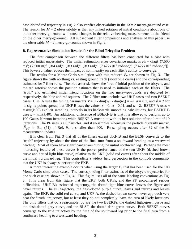
The relative rankings of the filters for the case in Fig. 4 are borne out by the 100-run Monte Carlo simulation tests. Figure 5 shows the computed RMS position error time history of each filter. It also shows results for the alternate PF with 10000 particles and a re-sampling threshold of effN̂ = 5000; these results are plotted as the dotted dark grey curve labeled PF B. The plotted value at each sample time tk is the corresponding RMS Δρxk value, computed as per Eq. (26), with the RMS computed by averaging over the 100 simulations. The best filter is BSEKF B (dash-dotted grey curve), and the worst is UKF B (dotted light-blue curve) for the first half and PF B (dotted dark-grey curve) for the last half. The ranking of the other filters from best to worst is BSEKF A (dashed light-green), EKF (solid red), UKF A (dashed brown) and PF (dash-dotted purple). The range of performance difference from the best to the worst filter is very large -- note the logarithmic vertical scale in the figure. Only the two BSEKF filters have reasonable performance, consistent with Fig. 4.

The BLSF is not included in this comparison because it is actually a smoother for all but its end point. It is plotted on Fig. 5 only for reference purposes. Its performance is better than that of any dynamic filter at initial sample t0 due to its smoothing nature and despite its lack of a process noise model or a priori information. Its performance is not as good as that of either BSEKF at the final sample t282 due to lack of a process noise model.

It is surprising that PF B performed worse than the original PF towards the end of the run. One would expect the greater number of particles in PF B to give it a clear advantage. Perhaps a factor of 3.3 increase in the number of particles is insufficient to ensure improvement in a 100-run Monte Carlo simulation. Alternatively, the dithering that is inherent in PF regularization could be interfering with the filter's accuracy convergence in the limit of a large number of particles.

24

0 50 100 150100

101

102

103

Time (sec)

RM

S P

ositi

on E

rror M

agni

tude

(m)

EKFUKF AUKF BPFPF BBLSFBSEKF ABSEKF B

Figure 5. Comparison of RMS position error time histories of filters computed from 100 Monte-Carlo simulations.

The time histories of the RMS values of the other error metrics in Eqs. (27) and (28), Δθxk and Δφxk, yield similar relative rankings between the filters. BSEKF B is the best and BSEKF A is second best. The EKF is next best in terms of RMS Δθxk heading error, but the EKF and UKF A are similar in terms of RMS Δφxk merry-go-round phase error. PF B is always the worst performer, and PF and UKF B are almost always in the group of worst performers. Similar rankings hold true when considering maximum error time histories maximized over the 100 Monte-Carlo cases instead of RMS time histories.

Another important evaluation metric is the required computation time of each filter. The PF and the BSEKF are much more complex computationally than are the EKF and the UKF. Therefore, any potential performance improvement must be weighed against the required computational resources. Consider the mean computation time in MATLAB on a 3 GHz 4-core Windows workstation per filtering run for the 100 cases. It was the following for the filter cases considered: EKF 0.0812 sec, UKF A 1.1821 sec, UKF B 1.1828 sec, PF 249.7 sec, PF B 680.9 sec, BSEKF A 60.84 sec, BSEKF B 110.62 sec. The maximum computation times over the 100 cases showed a similar trend: EKF 0.2434 sec, UKF A 1.2692 sec, UKF B 1.2258 sec, PF 314.6 sec, PF B 725.4 sec, BSEKF A 69.23 sec, BSEKF B 161.96 sec. Thus, the EKF had the fastest execution speed, and PF B was the slowest. Both PF and PF B were too slow, on average, to function in real-time because the total filtering interval was only 141 sec. All of the other filters showed potential for real-time operation, though BSEKF B was marginal in its ability to function in real-time. Given that PF and PF B had much worse accuracy than either BSEKF and given that the standard method for fixing such accuracy problems is to increase the number of particles, the PF seems clearly to be inferior to the BSEKF for this problem.

25

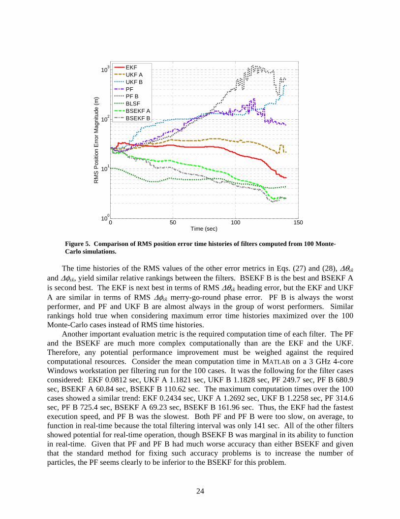
The reliability of the various filters' computed Pk covariance matrices are characterized by Fig. 6. It plots the fraction of the 100 cases that produced 2

kxχ from Eq. (29) that exceeded the 99.99% threshold value for a degree-7 distribution, i.e., that exceeded 29.8775. Nominally, this number should be 0.0001 for each plot. Given that the resolution is only 0.01 for 100 cases, this number should be zero on the plot. Obviously, it is significantly larger than this for all but a few cases at the start of the filtering interval, except that PF B shows reasonable values for most of the first half of the interval. The EKF (solid red curve) consistently has the worst performance, and PF B (dotted dark-grey curve) has the best performance. The two UKFs and the PF start with nearly the best performance, but their performance continuously degrades. The two BSEKFs show nearly the best performance by the end of the filtering interval, and it appears likely that they would overtake PF B if the interval were extended. In all cases except for the early PF B values, these results are far enough above 0.0001 to indicate problems with the computed Pk matrices, problems with the assumption of Gaussian behavior of the state errors, or both.

0 50 100 1500

0.1

0.2

0.3

0.4

0.5

0.6

0.7

0.8

0.9

1

Time (sec)

Frac

tion

of C

ases

EKFUKF AUKF BPFPF BBSEKF ABSEKF B

Figure 6. The various filters' fractions of cases in which 2

kxχ exceeds the 99.99% threshold for

a degree-7 χ2 distribution.

D. Monte-Carlo Results for Bi-Model 1-Dimensional Problems

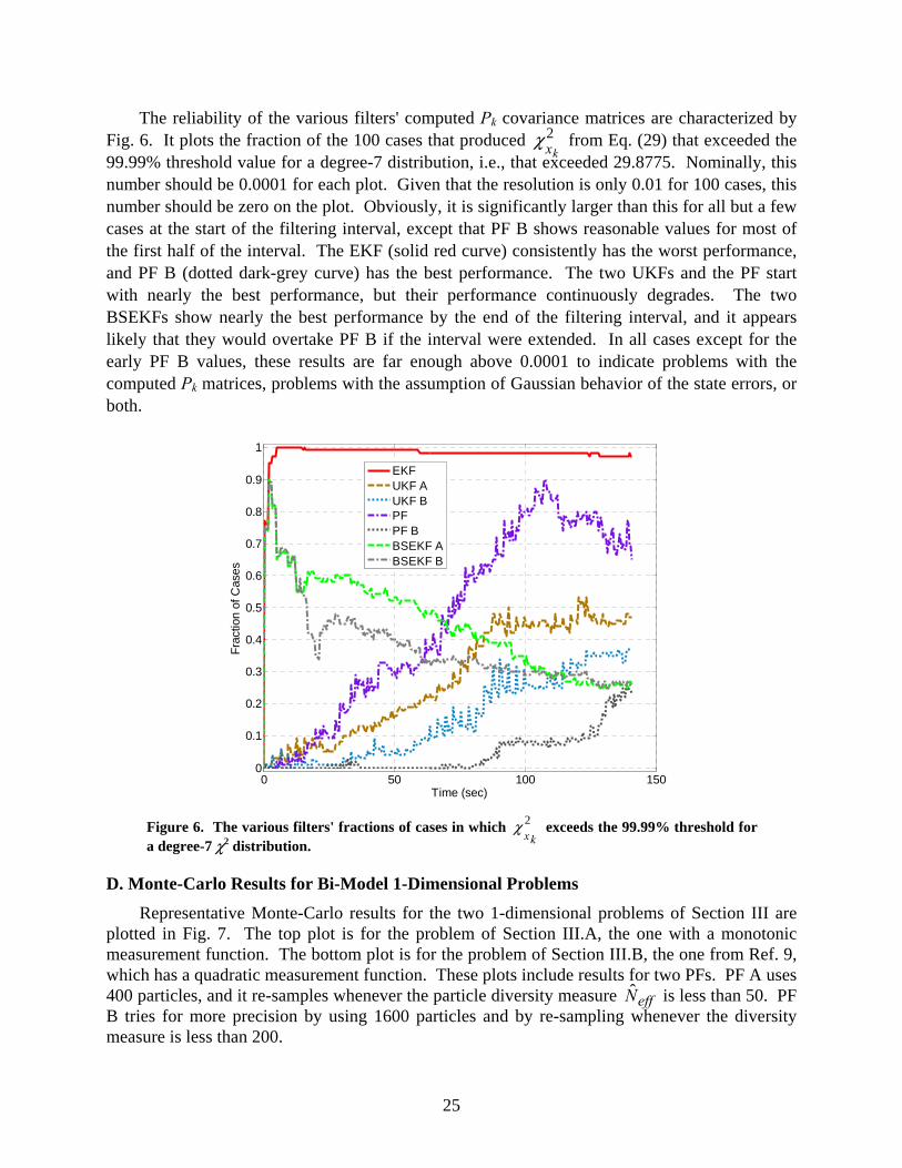
Representative Monte-Carlo results for the two 1-dimensional problems of Section III are plotted in Fig. 7. The top plot is for the problem of Section III.A, the one with a monotonic measurement function. The bottom plot is for the problem of Section III.B, the one from Ref. 9, which has a quadratic measurement function. These plots include results for two PFs. PF A uses 400 particles, and it re-samples whenever the particle diversity measure effN̂ is less than 50. PF B tries for more precision by using 1600 particles and by re-sampling whenever the diversity measure is less than 200.

26

0 10 20 30 40 50 60 70 80 90 10010-2

100

102

104

RM

S S

tate

Erro

r

0 10 20 30 40 50 60 70 80 90 100100

102

104

Sample Index k

RM

S S

tate

Erro

r

EKFUKF AUKF BPF APF BBSEKF ABSEKF B

Figure 7. Filter comparison of RMS state errors for 100 Monte-Carlo runs of the two bi-model 1-dimensional problems; top plot: first 1-D problem with monotonic measurement; bottom plot: second 1-D problem with quadratic measurement.

It is evident from the two plots that the EKF (red dots) and the two UKFs (brown x and light-blue +) have poorer performance than the two BSEKFs (light-green diamond and grey down-pointing triangle) and the two PFs (purple asterisk and dark-green up-pointing triangle). The two BSEKFs and the two PFs have nearly identical performance for the first example problem (top plot), but the two PFs clearly have superior accuracy for the second problem (lower plot). The maximum state errors maximized over the 100 Monte-Carlo cases yield similar relative results, except that a slight superiority of the PFs over the BSEKFs for the first example problem is somewhat more obvious from the maximal error time histories than from the RMS error time histories.

The counts of the times that the 2kxχ thresholds have been exceeded have been calculated

for these two cases. As per the discussion of Fig. 6 for the blind tricyclist problem, these can give an indication of how well each filter's Pk covariance matrix predicts its actual state estimation error statistics. The counts of violation of the 99.99% chi-squared threshold are consistent with theory for the two BSEKFs on the first 1-dimensional example. The PFs do not do as well on this example. For the second example, the roles are reversed. The two PFs are consistent with a true chi-square distribution, but the BSEKFs are much less consistent. The EKF has the poorest consistency for both example problems. The two UKFs have the next worst consistency.

Based on their accuracies and on their chi-squared consistencies, the BSEKFs are the best filters for the 1-D example problem with the monotonic measurement function, and the PFs are a close second. For the 1-D example problem with the quadratic measurement, on the other hand, the PFs are clearly the best filters, and the BSEKFs are a not-so-close second.

27

VII. Discussion Proponents of the UKF or the PF might feel that an unfair comparison has been made here,

especially for the blind tricyclist problem. One could try different κ, α, β tunings of the UKF's sigma-points spread in hopes of improving its performance. PFs can encounter difficulties when estimating constant parameters such as the merry-go-round rates 22. There are various other possible PFs besides the regularized PF defined in Refs. 5 and 9. One might try to develop a Rao-Blackwellized PF, as briefly discussed in Ref. 5, in hopes of reducing the dimensionality of the space in which particles are needed. Unfortunately, it is not obvious that Rao-Blackwellization can be applied to the blind tricyclist.

The UKF and PF implementations used in the present paper are only the most standard implementations, and more sophisticated ones may be available or under development. The author recommends that UKF and PF proponents apply any promising new versions of these filters to the blind tricyclist problem, treating it as a benchmark nonlinear estimation problem. The MATLAB functions and data file for the problem are available electronically in Ref. 21. If a successful UKF or PF can be developed for the case of large initial state uncertainty, then that result should be publishable.

At this point, there does not appear to be any one filter that performs well in all situations. The BSEKF seems to come nearest to this ideal, but its performance was unsatisfactory on the second 1-dimensional problem, and its covariance consistency was poor on the blind tricyclist problem. Therefore, further improvements in nonlinear filtering algorithms should be pursued. The following are several possible avenues of development.

Gaussian mixture filters 10,11 could be improved by having a better re-sampling method that would keep the distribution widths bounded to allow EKF or UKF propagation, as has been attempted in Ref. 12. The result might be a generalization of the particle filter that replaced infinitesimal-width particles with Gaussian components of finite covariance. The hope would be to achieve good nonlinear performance with orders of magnitude fewer Gaussian components than particles because each such component and its weight would carry much more information.

Another possibility is to use a combination of BSEKF techniques and PF techniques. BSEKF calculations could be used to generate proposal distributions for the PF that were fairly near the true distribution. This would represent an extension of known methods that use an EKF, a UKF, an IEKF, or an iterated UKF to generate the proposal distributions 23. This extension might allow accurate PF calculations with many fewer samples. It also might improve on the BSEKF covariance calculations. PF techniques, in turn, could help BSEKF calculations by providing seed guesses for its iterative nonlinear backwards smoothing problems that might help it to locate multiple modes if they existed. These first guesses would be in addition to the first guess near the solution of the problem associated with the previous sample.

It might be possible to incorporate UKF techniques into the BSEKF iterative nonlinear smoothing calculations. There already exists a UKF smoother 24. If this smoother could be adapted to iteratively improve its approximations of the underlying nonlinearities, then it could be used to solve each backwards smoothing problem of the BSEKF. This could give two advantages to the BSEKF. First, it would not need to used explicitly computed Jacobian matrices Φk, Γk, and Hk. Second, the convergence would likely be improved due to the usual second-order information contained in the UKF. This second-order information might also improve the convergence speed of the iterative nonlinear smoothing calculations.

28

An alternative improvement to the BSEKF would be to directly incorporate second derivative information. This would speed the convergence of each nonlinear smoothing solution, thereby reducing computational requirements. It could also improve the BSEKF covariance estimate. Such an approach would have the effect of making the modeling more difficult by requiring explicit Hessians of the components of the problem model functions fk and hk.

VIII. Conclusions This paper has developed a new example nonlinear filtering problem, and it has used this

new problem and two other problems to compare the performance of a number of nonlinear filters. The new problem is called the blind tricyclist problem. It involves a sightless tricyclist who peddles around an amusement park while deriving navigation information from the relative bearing measurements to friends who periodically shout to him from merry-go-rounds. The tricyclist must estimate his east/north position and his heading plus each friend's merry-go-round rotation angle and rate. The problem is observable with 2 or more merry-go-round riding friends, but it has significant nonlinearities that pose challenges to standard nonlinear estimation schemes.

The blind tricyclist problem has been used to compare the performance of 5 filters. They are the extended Kalman filter, the unscented Kalman filter, a regularized version of the particle filter, a batch least-squares filter, and a new filter called the backwards smoothing extended Kalman filter. The filters all perform reasonably well on the 2-merry-go-round blind tricyclist problem when the initial state uncertainty is moderate. When the initial uncertainty becomes too large, however, only the batch least-squares filter and the backwards smoothing extended Kalman filter show good performance. Surprisingly, the extended Kalman filter, although not good, was not the worst of the filters.

The backwards smoothing filter is computationally expensive because it solves a moving horizon nonlinear least-squares smoothing problem at each measurement update. Despite its complexity, the backwards smoothing algorithm requires significantly less computation time than corresponding particle filters while yielding a better solution.

The particle filter performed as well as or better than the backwards smoothing extended Kalman filter on two simpler example problems. The two filters' performance was nearly equal on one of the problems, but the particle filter was much better than the backwards smoothing filter on the other problem.

Thus, no one filter dominates as a sure solution to all nonlinear estimation problems. The discipline of nonlinear estimation is one in which new developments have the potential to make significant improvements towards the goal of developing a generally applicable algorithm.

References

1. Kalman, R.E., "A New Approach to Linear Filtering and Prediction Problems," Trans. ASME Journal of Basic Engineering, Vol. 82, March 1960, pp. 34-45.

2. Kalman, R.E., and Bucy, R., "New Results in Linear Filtering and Prediction Theory," Trans. ASME Journal of Basic Engineering, Vol. 83, March 1961, pp. 95-108.

3. Brown, R.G., and Hwang, P.Y.C., Introduction to Random Signals and Applied Kalman Filtering, 3rd Edition, J. Wiley & Sons, (New York, 1997), pp. 345-346.

29

4. Bar-Shalom, Y., Li, X.-R., and Kirubarajan, T., Estimation with Applications to Tracking and Navigation, J. Wiley & Sons, (New York, 2001), pp. 92-98, 381-395, 404-409, 441-466.

5. Ristic, B., Arulampalam, S., and Gordon, N., Beyond the Kalman Filter, Artech House, (Boston, 2004), pp. 19-22, 24-31, 35-60, 94-98.

6. Julier, S., Uhlmann, J., and Durrant-Whyte, H.F., "A New Method for the Nonlinear Transformation of Means and Covariances in Filters and Estimators," IEEE Transactions on Automatic Control, Vol. AC-45, No. 3, 2000, pp. 477-482.

7. Wan, E.A., and van der Merwe, R., "The Unscented Kalman Filter," Kalman Filtering and Neural Networks, S. Haykin, ed., J. Wiley & Sons, (New York, 2001), pp. 221-280.

8. Gordon, N.J., Salmond, D.J., and Smith, A.F.M., "Novel Approach to Nonlinear/Non-Gaussian Bayesian State Estimation," IEE Proceedings-F, Radar and Signal Processing, Vol. 140, No. 2, 1993, pp. 107-113.

9. Arulampalam, M.S., Maskell, S., Gordon, N., and Clapp, T., "A Tutorial on Particle Filters for Online Nonlinear/Non-Gaussian Bayesian Tracking," IEEE Transactions on Signal Processing, Vol. 50, No. 2, Feb. 2002, pp. 174-188.

10. Sorenson, H.W., and Alspach, D.L., "Recursive Bayesian Estimation Using Gaussian Sums," Automatica, Vol. 7, No. 4, 1971, pp. 465-479.

11. van der Merwe, R., and Wan, E., "Gaussian Mixture Sigma-Point Particle Filters for Sequential Probabilistic Inference in Dynamic State-Space Models," Proceedings of the International Conference on Acoustics, Speech and Signal Processing, (Hong Kong), IEEE, Apr. 2003. Available at http://www.cse.ogi.edu/~rudmerwe/pubs/index.html.

12. Psiaki, M.L., Schoenberg, J.R., and Miller, I.T., "Gaussian Mixture Approximation by Another Gaussian Mixture for 'Blob' Filter Re-Sampling," AIAA Paper No. 2010-7747, Proc. AIAA Guidance, Navigation, and Control Conf., Aug. 2-5, 2010, Toronto, Canada.

13. Psiaki, M.L., "Backward-Smoothing Extended Kalman Filter," Journal of Guidance, Control, and Dynamics, Vol. 28, No. 5, Sept.-Oct. 2005, pp. 885-894.

14. Crassidis, J.L., and Markley, F.L., "Unscented Filtering for Spacecraft Attitude Estimation," Journal of Guidance, Control, and Dynamics, Vol. 26, No. 4, 2003, pp. 536-542.

15. Moon, F.C., Chaotic Vibrations, J. Wiley & Sons, (New York, 1987), pp. 77-79. 16. Bierman, G.J., Factorization Methods for Discrete Sequential Estimation, Academic Press,

(New York, 1977), pp. 69-76, 115-122, 214-217. 17. Psiaki, M.L., Theiler, J., Bloch, J., Ryan, S., Dill, R.W., and Warner, R.E., “ALEXIS

Spacecraft Attitude Reconstruction with Thermal/Flexible Motions Due to Launch Damage,” Journal of Guidance, Control, and Dynamics, Vol. 20, No. 5, Sept.-Oct. 1997, pp. 1033-1041.

18. Brunke, S., and Campbell, M.E., "Square Root Sigma Point Filtering for Real-Time, Nonlinear Estimation," Journal of Guidance, Control, and Dynamics, Vol. 27, No. 2, 2004, pp. 314-317.

19. Gill, P.E., Murray, W., and Wright, M.H., Practical Optimization, Academic Press, (New York, 1981), pp. 133-141.

20. Tapley, B.D., Schutz. B.E., and Born, G.H., Statistical Orbit Determination, Elsevier, (New York, 2004), pp. 159-261.

30

21. Psiaki, M.L., "Blind Tricyclist Problem MATLAB Functions and Example Input/Output Data File," available at URL http://web.mae.cornell.edu/psiaki/blind_tricyclist_ modeling_and_sim_fncts_and_example_data.zip, Oct. 2011.

22. Djuric, P.M., Bugallo, M.F., and Miguez, J., "Density Assisted Particle Filters for State and Parameter Estimation," Proc. IEEE Int'l. Conf. on Acoustics, Speech, and Signal Processing (ICASSP '04), Vol. 2, Montreal, Canada, 17-21 May 2004, pp. 701-704.

23. Cao, H., Ohnishi, N., Takeuchi, Y., Matsumoto, T., and Kudo, H., "Gauss-Newton Particle Filter," IEICE Transactions on Fundamentals of Electronics, Communications and Computer Sciences, Vol. E90-A, No. 6, June 2007, pp. 1235-1239.

24. Psiaki, M.L., and Wada, M., "Derivation and Simulation Testing of a Sigma-Points Smoother," Journal of Guidance, Control, and Dynamics, Vol. 30, No. 1, Jan.-Feb. 2007, pp. 78-86.