The Benefits of Mandatory Disclosure: Evidence from ...

The Benefits of Mandatory Disclosure: Evidence from Regulation S-X Article 11

Matthew Kubic*

Duke University

[email protected]

January 20, 2020

ABSTRACT

The SEC mandates disclosure of Article 11 pro forma financial statements (pro formas) for

acquisitions that exceed one of three bright-line materiality thresholds. Motivated by two theories

of mandated disclosure, I test whether pro formas improve analyst forecasts or mitigate incentive

alignment problems. Using a fuzzy regression discontinuity design, I provide evidence that pro

formas reduce post-acquisition forecast errors and improve target selection. The improvement in

forecast accuracy (target selection) is concentrated in acquirers with low analyst following

(acquisitions involving third-party advisors), suggesting that benefits to mandated pro forma

disclosure depend on the pre-existing information environment.

Keywords: accuracy enhancement; acquisition; incentive alignment; pro forma disclosure

* I thank my dissertation committee members Scott Dyreng, Elisabeth de Fontenay, Bill Mayew (co-

chair), and Katherine Schipper (co-chair) for their support and guidance. I thank Oliver Binz, Robert Hills, Duncan Thomas, Xu Jiang, and workshop participants at Duke University and the 2019 AAA/ Deloitte Foundation/ J. Michael Cook Doctoral Consortium for helpful comments and suggestions. I thank Daniel Giron, Katherine Guo, and Hyun Kwon for their assistance in data collection. All errors

are my own.

1

I. INTRODUCTION

Few transactions generate as much public attention and academic research as mergers

and acquisitions (M&A) (Betton et al. 2008). M&A generates significant gains or losses for

shareholders (Moeller et al. 2005), reallocates resources within the economy, generates billions

in annual advisory fees (Golubov et al. 2012), and increases uncertainty (Erickson et al. 2012).

Acquiring firms spend significant resources to obtain information about target quality, identify

and estimate synergies, and forecast results of the combined enterprise, resulting in asymmetric

information between managers and shareholders (Li et al. 2018; Golubov et al. 2012). Prior

research shows asymmetric information and incentive misalignment play an important role in

explaining acquisition structure (Travlos 1987), the allocation merger gains (Betton et al. 2008),

the existence of fairness opinions (Kisgen and Song 2009), shareholder voting (Li et al. 2018),

and governance mechanisms (Masulis et al. 2007). Article 11 of Regulation S-X (Article 11)

requires SEC registrants to provide pro forma financial information for acquisitions that exceed

one of three 20% materiality thresholds based on the relative sizes of the bidder and target (the

asset test, income test, and investment test). Bidders whose acquisitions lie just above the

threshold are required to provide pro formas, while otherwise similar bidders whose acquisitions

lie just below the threshold have no required disclosure. For acquisitions with required pro

forma disclosure, the acquirer must provide an as-if consolidated balance sheet and income

statement, with separate columns presenting historical acquirer financial statements, historical

target financial statements, pro forma adjustments, and pro forma results. The economic

importance of M&A, combined with disclosure rules that apply only to certain acquisitions,

make the setting well-suited for testing the benefits of event-based mandated disclosure.

2

Prior literature considers at least two objectives of disclosure regulation. First, the

accuracy enhancement hypothesis posits that mandatory disclosure provides information that is

useful in valuing securities, and absent a mandate, firms would not provide the information

(Coffee Jr 1984; Admati and Pfleiderer 2000). Under this hypothesis, the requirement to provide

pro forma disclosure does not affect an acquirer’s acquisition decision but does affect market

participants’ ability to value the combined enterprise. Second, the incentive alignment

hypothesis posits that mandated disclosure alleviates an agency problem by aligning incentives

(Mahoney 1995). Managers may wish to invest in low-quality projects rather than return capital

to shareholders (Jensen 1986; Chen 2019), or managers may face perverse incentives as the

capital market is less informed (Kanodia and Lee 1998). If managers lack acquisition expertise,

they may hire an outside advisor, such as an investment bank, who receives a contingent fee on

deal closing, creating misaligned incentives (Mahoney 1995; Buffett 2018). Mandated

disclosure may alleviate these problems by increasing transparency and reputational concerns

(Chemmanur and Fulghieri 1994), or by providing an ex post measure of target selection which

disciplines ex ante investment decisions (Kanodia and Lee 1998). Under the incentive alignment

hypothesis, firms modify acquisition decisions (e.g., choose different targets, adjust payment

terms, etc.) knowing that pro formas will provide transparency into target selection. Prior

research (Bushman et al. 2006; Mahoney 1995; Paul 1992; Gjesdal 1981) shows that mandated

disclosure theories may be complementary, competing, or independent, which suggests that I

may find support in favor of both, one, or neither hypothesis.

I test my hypotheses using a sample of 3,080 acquisitions between 2002 and 2016, with

an aggregate transaction consideration of over 2 trillion dollars. To address endogeneity

concerns, I use a fuzzy regression discontinuity (RD) design around the 20% investment test

3

threshold. Below the 20% investment threshold, only 19.5% of acquirers file pro formas, either

voluntarily or because they cross another unobservable threshold. Above the investment test

threshold, 94.6% of acquirers file pro formas.

First, I test the accuracy enhancement hypothesis that pro formas improve market

participants’ ability to forecast future earnings, consistent with the SEC’s claim that pro formas

help investors predict the “financial condition and results of operations of the combined entity

following the acquisition” (SEC 2015). Under the null hypothesis, firms have strong incentives

to provide informative voluntary disclosure (Grossman 1981; Grossman and Hart 1980) and,

even in the absence of full disclosure, it is unlikely that mandated uniform disclosure will

provide precisely the type of information that is needed to forecast future earnings (Stigler 1964;

Mahoney 1995). Moreover, pro forma disclosure is unaudited, does not contain a forecast, and

only allows for the presentation of factually supportable synergies, which may limit its

usefulness (CFA Institute 2016; SEC 2019). Finally, the existing information environment,

including other mandated filings and information produced by other market participants, may

already contain all information included in Article 11 pro formas, leading to the prediction that

forecasting benefits depend on the amount of information produced absent a mandate.

I test the accuracy enhancement hypothesis by examining analyst forecast errors in the

post-combination period. I show that forecast errors increase in the post-acquisition period, and

using a fuzzy RD design, I provide evidence pro formas mitigate the increase in post-acquisition

analyst forecast errors. The coefficient magnitudes suggest that for acquisitions right above the

20% threshold, the provision of pro formas may fully offset the increase forecast errors. I show

the results are robust to weighting observations, alternative specifications, and two measures of

common and total uncertainty from Barron et al. (1998).

4

I conduct two tests to determine whether the forecasting benefit of pro formas depends

on the pre-existing information environment. First, I split the sample by analyst following and

find a forecasting benefit only for firms with below-median analyst following. This result

suggests that information necessary to forecast earnings is produced even without a disclosure

mandate for firms with above-median analyst following. Second, I examine the effect of pro

formas on forecast errors for different target types as forecasting difficulty may vary with target

pre-acquisition information. I find a negative association between pro formas and three (two of

three) outcome measures in the subsample of private and subsidiary targets (public targets).

Overall, the evidence is consistent with the accuracy enhancement hypothesis.

Next, I test whether pro forma disclosure mitigates an incentive alignment problem by

providing information about target selection. I define high (low) quality target selection as

acquisitions with a higher (lower) net present value. Following Bao and Edmans (2011), I use 3-

day announcement returns as a proxy for target quality and show pro forma income statement

metrics (pro forma EPS, purchase price to revenue, and pro forma operating margin) explain

variation in announcement returns. Using multiple specifications, I show that the provision of

pro formas is associated with higher quality target selection. I show this result is concentrated in

acquisitions of non-public targets involving an outside advisor, and I find that acquirers using an

outside advisor are less likely to complete acquisitions that are accretive to pro forma EPS.

Overall, the evidence is consistent with mandated pro forma disclosure mitigating an incentive

problem between outside advisors and shareholders by improving transparency.

While mandated disclosure is a first-order policy issue (Stigler 1964; Coffee Jr 1984;

Leuz and Wysocki 2016), Healy and Palepu (2001) note limited research on disclosure regulation

before 2000. Leuz and Wysocki (2016) review a growing number of regulatory studies focused

5

on a small number of well-known changes in the 2000s (IFRS adoption, Regulation FD, or

Sarbanes-Oxley) and discuss inference limitations due to commonalities in design. In many

cases, regulatory changes are in response to a financial or economic crisis (e.g., Enron), occur at

the same time as other institutional changes (e.g., changes in enforcement as discussed in

Christensen et al. (2013)), and apply to most firms in an economy making it difficult to identify

counterfactuals. I contribute to this literature by studying a new type of disclosure mandate, in a

new setting, using a design with different strengths and weaknesses. With regard to limitations,

the main concern is that acquirers manipulate transactions to avoid the threshold. While I make

research design choices to mitigate the possibility of manipulation and conduct tests to address

the concern, I cannot rule out a selection or manipulation threat. Moreover, the choice of a

bandwidth requires a tradeoff between sample size and comparability of acquisitions. With

regard to strengths, treatment occurs consistently throughout my sample period, reducing validity

threats from contemporaneous economic shocks or changes in enforcement, and across the

spectrum of firm size and characteristics. A large firm with high analyst following could be a

treatment firm in one year and a control firm in the next year. By conducting both large-sample

tests focused on identification and subsample analysis using hand-collected disclosure, I am able

more closely link disclosure attributes to outcomes. Finally, this setting allows for

diversification of empirical evidence and helps identify the conditions under which disclosure

regulation is, or is not, likely to improve outcomes (Leuz and Wysocki 2016).

My paper makes the following contributions. First, the SEC is considering amendments

to the pro forma guidance as part of a larger project on disclosure effectiveness, and there is no

academic research on the costs or benefits of pro formas (SEC 2015, 2019). I provide evidence

on potential benefits of pro forma disclosure, which may be useful to the SEC (Leuz 2018).

6

Second, I contribute to the literature on mandated financial disclosure by examining event-based

pro forma disclosure (Stigler 1964; Benston 1969; Bushee and Leuz 2005; Greenstone et al.

2006). I provide evidence on the forecasting (Ramnath et al. 2008) and incentive alignment

(Jensen 1986; Mahoney 1995; Chen 2019) benefits of pro forma disclosure and contribute to the

literature on M&A advisors (Bao and Edmans 2011; Golubov et al. 2012). My incentive

alignment tests compliment Chen (2019), who shows Rule 3-05 disclosure of target historical

financial is associated with better post-acquisition operating performance. Finally, I contribute to

the literature on acquisition announcement returns by showing that pro forma metrics, which

exclude anticipated synergies, explain variation in announcement returns (Betton et al. 2008).

This study proceeds as follows. Section 2 provides background, Section 3 discusses

hypothesis development and Section 4 provides sample selection. Section 5 tests accuracy

enhancement, section 6 tests incentive alignment, and Section 7 concludes.

II. BACKGROUND ON ARTICLE PRO FORMA DISCLOSURE

In 1982, the SEC added Article 11 to Regulation S-X (Article 11). Article 11 requires

SEC registrants to provide pro forma financial information, including a balance sheet, income

statements, and footnotes, for material transactions. The objective of pro forma information is to

“help investors understand the impact of a significant transaction, such as a business

combination or disposition, by showing how it might have affected the historical financial

statements (Young 2016).” In this paper, I focus on M&A pro forma disclosures.

The SEC and FASB acknowledge that “information about a reporting entity is more

useful if it can be compared with similar information about other entities and with similar

information about the same entity for another period or another date (FASB 2010, QC 20).”

After an acquisition, the post-acquisition financial statements of the acquirer are less comparable

7

to prior periods. To improve comparability, the SEC mandates disclosure of pro forma

information, specifically, an as-if consolidated balance sheet and income statement, with

separate columns presenting historical financial statements of the acquirer, historical financial

statements of the target, pro forma adjustments, and pro forma results (Young 2016). Article 11

requires disclosure of pro forma financial information when an acquisition is probable or

completed. The form requiring pro forma disclosure depends on the nature of the transaction. In

transactions requiring a vote by the shareholders (Li et al. 2018), or requiring the registration of

new shares (Deloitte 2018), acquirers provide Article 11 pro formas in the prospectus or

registration statements (typically, a Form S-4). In these cases, investors have access to pro

forma financial statements before the acquisition closing. In addition, firms must file pro formas

in a Form 8-K within 4 business days of acquisition closing, with an optional 71 calendar day

extension. If the acquirer files pro formas before acquisition closing, either in Form 8-K or a

registration statement, the acquirer may file updated pro formas in the post-closing period or may

incorporate by reference the previous pro formas. The SEC requires Article 11 pro forma

disclosure if an acquisition is material at the 20% threshold under the following 3 tests:

Asset Test – The ratio of the target’s pre-acquisition assets to the acquirer’s pre-

acquisition assets, as of the most recently completed fiscal year.

Investment test – The ratio of the purchase price, as defined in US GAAP, to the

acquirer’s pre-acquisition total assets.

Income test – The ratio of the target’s income before taxes to the acquirer’s income

before taxes, subject to certain adjustments.1

Pro forma financial statements are required if the largest ratio from the three tests is greater than

20%. Registrants must provide the same pro forma information, whether barely exceeding one

1 Income in this test is defined as the absolute value of “income from continuing operations before income taxes,

extraordinary items and cumulative effect of a change in accounting principle (Young 2016).” If current acquirer

income is 10% less than the 5 year average, then the 5 year average should be used (SEC 2015).

8

threshold or greatly exceeding all three thresholds. While some firms may voluntarily provide

pro formas, other firms with an obligation to provide pro formas may seek relief from the SEC.

Pro forma financial statements require condensed presentation of the income statement

and balance sheet, including columnar presentation of the following:

Historical financial statements of the acquirer

Historical financial statement of the target

Pro-forma adjustments

Pro-forma results that reflect the sum of the historical financial statements and pro

forma adjustments

For public acquirers, the historical financial statements are already publicly available, and the

availability of pre-acquisition target financial statements depends on the target’s pre-acquisition

reporting requirements. If the historical financial statements of the target are not publicly

available, Rule 3-05 requires the acquirer to disclose audited financial statements of the target.2

Target financial statements reflect the target’s historical accounting and may be prepared in a

different currency, using a different basis of GAAP, and in certain situations, current practice

allows for abbreviated presentation (Young 2016; Deloitte 2018; SEC 2019; Young 2019).

Adding the target and acquirer’s historical financial statements will not result in a balance sheet

or income statement that is comparable to the combined entity, as the acquirer must apply

purchase accounting, and certain known adjustments will cause historical financial statements to

differ from future financial statements. To address these issues, a pro forma adjustment column

presents adjustments that meet the following criteria:

1. Directly attributable to the transaction

2. Have a continuing effect on income, and

3. Factually supportable

2 Unlike Rule 3-05 financial statements, Article 11 pro formas are unaudited. While not subject to an audit, the

registrant’s auditor must still comply with professional auditing standards (for example, PCAOB AU 550 requires

auditors to review pro formas to ensure they are not “inconsistent” with the audited financial statements), and

auditors may perform procedures requested by 3rd parties (e.g. comfort letters). (Young 2016)

9

While the most common pro forma adjustment is the application of purchase accounting, firms

recognize pro forma adjustments for other known changes, such as adjustments to capital

structure.3 The directly attributable criterion requires adjustments to be directly related to the

acquisition. For example, suppose a firm incurs a large restructuring expense and then

completes an unrelated acquisition. The directly attributable criterion prohibits a pro forma

adjustment to remove the restructuring expense, as it is not directly attributable to the

acquisition. The 2nd criterion requires pro forma adjustments to have a continuing effect on

income. Pro forma income statements exclude transaction costs, inventory fair value

adjustments, and short-term favorable/unfavorable contract amortization. The 3rd criterion,

factually supportable, is the most contentious as it prevents registrants from including anticipated

synergies as they are not factually supportable (Young 2016).4

Appendix A provides an illustrative example of a pro forma income statement for the

AT&T acquisition of DirectTV. Since DirectTV was a public company prior to the acquisition,

the only new information contained in the disclosure is pro forma adjustments. Examples of

AT&T pro forma adjustments include conforming accounting policies, eliminating intercompany

sales, and applying purchase accounting (AT&T 2015). Since purchase accounting is not

complete, AT&T shows how property, plant, and equipment fair value changes will affect future

depreciation. Since AT&T financed the acquisition with debt and equity, AT&T shows the new

interest expense and the effect of equity issuances on earnings per share (AT&T 2015).

3 The E&Y business combination guidance provides illustrative examples of 18 different types of pro forma

adjustments in business combinations, including the treatment of transaction costs, compensation, disposals, taxes,

restructuring, accounting policy changes, impairment, deferred revenue, and inventory valuation (Young 2016). 4 In 2015, the SEC issued a request for feedback on the usefulness of pro formas (SEC 2015). Several respondents

raised concerns about the application of the factually supportable criterion (Respondents 2015). These

respondents stated that pro formas would be more useful if firms were permitted to include adjustments met some

lower standard such as “reasonably estimable and reasonably expected to occur” (Young 2019; SEC 2019).

10

III. HYPOTHESIS DEVELOPMENT AND RESEARCH DESIGN

While there is no current unifying theory that explains the problem solved by mandated

disclosure (Verrecchia 2001; Beyer et al. 2010), securities laws in most developed economies

require extensive disclosure (Mahoney 2009; Berger 2011). The benefits to mandatory

disclosure are widely debated and depend on the information produced absent a mandate (Stigler

1964; Coffee Jr 1984; Mahoney 2009; Dye 1990). The empirical literature on mandated

disclosure begins with research on the Securities Act of 1933 and the Exchange Act of 1934 (the

Securities Acts). While early academic research generally found no benefit to the Securities

Acts (Stigler 1964; Benston 1969, 1973), later critiques discuss methodological concerns and

design limitations that limit inferences (Friend and Herman 1964; Seligman 1983). Subsequent

research tests the market response to expanding the Securities Acts to OTC or OTCBB firms

(Greenstone et al. 2006; Bushee and Leuz 2005). While Greenstone et al. (2006) find a positive

market response to mandated disclosure regulation, Bushee and Leuz (2005) document a

negative market response, and show 76% of firms choose to delist, suggesting that costs

outweigh the benefits for firms of a certain size.5

Prior research on mandated disclosure in an M&A setting focuses on the 1968 Williams

Act issued in response to perceived abuses, such as “Saturday night raids,” where acquirers

secretly purchased shares from large blockholders. Congress passed the Williams Act to protect

target shareholders by requiring an orderly auction process (e.g., minimum 20 day offer period)

and mandating disclosure in a Form 14D (Betton et al. 2008). Research on the Williams Act

documents higher target premiums (Jarrell and Bradley 1980) and a reduction to quasi-rents

5 The studies compare newly regulated OTC or OTCBB firms to existing SEC registrants. Greenstone et al. (2006)

suggest that differences in results are due to differential size of treatment firms, as their average (median)

treatment firm is approximately 7 (8) times larger than the treatment firms in Bushee and Leuz (2005).

11

available to acquirers (Schipper and Thompson 1983), but is unable to determine whether the

effects are due to mandated disclosure or changes in the tender process (Betton et al. 2008). My

study examines one type of disclosure mandated by the Securities Acts not explored in prior

literature, the requirement to provide event-based Article 11 pro formas.

Two common explanations for mandated disclosure are accuracy enhancement (Coffee Jr

1984; SEC 2013; Admati and Pfleiderer 2000; Barth et al. 2001) and incentive alignment

(Mahoney 1995; Kothari et al. 2010). Prior research on disclosure regulation usually focuses on

capital market effects, such as improved liquidity or forecasting ability, or real effects (Healy

and Palepu 2001; Leuz and Wysocki 2016). Similarly, I use these two theories to motivate my

hypotheses on mandated pro forma disclosure. Analytical research shows that it is possible to

have a financial measure that is useful for valuing the firm but not addressing agency problems

(Paul 1992; Gjesdal 1981; Lambert 2001, Section 3.5). Mahoney (1995, 2008) argues that

accuracy enhancement and agency cost are competing hypotheses, while Bushman et al. (2006)

show a positive association between the value of earnings in valuation and contracting,

suggesting the possibility of complementarities. Based on these differing perspectives, it seems

possible that I may find support for one hypothesis, both hypotheses, or neither hypothesis.

The Accuracy Enhancement Hypothesis

The accuracy enhancement hypothesis argues a market failure prevents voluntary

disclosure of all information necessary to price securities and that the purpose of mandated

disclosure is to provide information that is useful in determining the value of the firm.6 Given

the link between earnings and firm value (Ohlson 1995), I test whether pro forma information

6 Coffee Jr (1984) and Simon (1989) argue that financial information is similar to a public good and the free-rider

problem may lead to underproduction. Easterbrook and Fischel (1996) argue that free-rider problems are more

prominent when information produced by one firm is used by investors of another firm. Verrecchia (1983) shows

disclosure may reveal proprietary information which prevents full unraveling.

12

improves market participants’ ability to forecast earnings, consistent with the SEC’s claim that

pro formas help investors predict the “financial condition and results of operations of the

combined entity (SEC 2015).” Following prior literature (Bradshaw et al. 2017), I use analyst

forecasts as a proxy for the market’s expectation of future earnings. The pro forma requirement

to only include items with a recurring effect on income appears consistent with analyst forecasts,

which often exclude transitory items (Bradshaw et al. 2018). In addition, there is anecdotal

evidence that analysts use pro formas. When discussing the AT&T acquisition of Time Warner,

Bank of America analyst David Barden stated: “We expect AT&T to file pro forma financial

statements in the coming weeks which should improve Street models… and add conviction to

numbers” (Franck 2018). This reasoning leads to my first hypothesis:

H1A: Article 11 pro forma financial statements reduce analyst forecast errors

There are several reasons why Article 11 pro forma disclosure may not reduce analyst forecast

errors. First, pro formas are unaudited, and investors may have concerns about reliability.7 If the

purpose of mandatory disclosure is to confirm more informative voluntary disclosure, then

unaudited pro forma disclosure may provide little value (Gigler and Hemmer 1998). Second,

some view the current pro forma requirements as too restrictive to be useful. For example, the

CFA stated, “investors are primarily interested in understanding how a company will look going

forward… Thus, the current limitations on significant planned changes by the acquirer, such as

workforce reductions, facility closings, actually hinder, rather than help, the investor (CFA

Institute 2016).” Third, firms may provide more informative voluntary disclosure (Grossman

and Hart 1980; Grossman 1981). Even if firms do not disclose all relevant information, prior

7 Teoh and Wong (1993) show equity investors place more weight on audited earnings, and Francis et al. (1999)

show that high quality auditors are associated with more credible reporting.

13

literature argues that it is unlikely that a regulator can design a uniform disclosure rule requiring

precisely the type of information that investors need to forecast earnings, but firms wish to

withhold (Stigler 1964, 1971; Mahoney 1995). Finally, the existing information environment

may already contain all information included in Article 11 pro formas. In addition to Article 11

pro formas, firms must file merger agreements in a Form 8-K, and ASC 805-10-50, Business

Combinations requires disclosure of the purchase price allocation, pro forma revenue, and pro

forma earnings calculated on a different basis.8 Market participants, including sell-side analysts,

have strong incentives to gather information, raising the possibility that market participants

produce information contained in pro formas even absent a mandate (Bradshaw et al. 2017;

Kothari et al. 2016; Grossman and Stiglitz 1980). Moreover, some targets are publicly traded

and covered by analysts before the acquisition. Thus, the forecasting benefit to pro formas may

depend on the pre-existing information environment, which leads to the following hypothesis:

H1B: The effect of Article 11 pro forma financial statements on analyst forecast errors

depends on the pre-existing information environment of the target and acquirer

The Incentive Alignment Hypothesis

Prior academic literature discusses two potential incentive problems in an M&A setting.

First, managers with misaligned incentives may wish to invest in low-quality projects rather than

return capital to shareholders (Jensen 1986; Morck et al. 1990; Chen 2019). Second, managers

may lack acquisition experience and hire an outside advisor whose incentives are not aligned with

shareholders (Mahoney 1995; Kosnik and Shapiro 1997; Buffett 2018). Both of these incentive

problems may lead to acquisitions with a lower net present value or internal rate of return, the two

8 Ernst and Young describe ASC 805 pro formas as “different from and substantially less detailed than the

information required [by] Article 11” and the PwC Business Combination guide discusses differences in format,

content, the level income statement disaggregation, and treatment of non-recurring transactions (PwC 2014).

14

most common metrics used by managers to evaluate investment projects (Graham and Harvey

2001). Warren Buffet expressed similar concerns in his 2017 shareholder letter:

"Once a CEO hungers for a deal, he or she will never lack for forecasts that justify the purchase.

Subordinates will be cheering, envisioning enlarged domains and the compensation levels that

typically increase with corporate size. Investment bankers, smelling huge fees, will be applauding

as well. (Don’t ask the barber whether you need a haircut.) If the historical performance of the

target falls short of validating its acquisition, large “synergies” will be forecast.” (Buffett 2018)

Mahoney (1995) argues the purpose of mandated disclosure is to reduce agency conflicts,

and that information designed to address agency problems should be limited in scope, precise,

and not overly costly to produce. These criteria appear consistent with pro forma disclosure,

which is substantially shorter than periodic financial statements, the factually supportable

criterion ensures that adjustments have high precision, and pro forma information is potentially a

subset of the entire information set management used to evaluate the acquisition and thus not

overly costly to produce. Kanodia and Lee (1998) show disclosure that helps investors identify

low-quality investment ex post will discipline managers’ ex ante investment choices. Consistent

with this framework, Chen (2019) shows that acquirers who provide target audited financial

statements experience better post-acquisition fundamental performance (ROA, 3-year abnormal

returns, and lack of goodwill impairment). Chemmanur and Fulghieri (1994) show reputational

concerns can alleviate an incentive problem between shareholders and the 3rd party advisors.

Shareholders may evaluate the target quality using pro forma information, leading to increased

transparency and reputational concerns.9 This reasoning leads to my second set of hypotheses:

H2A: Article 11 pro forma financial statements mitigate an incentive alignment problem

between managers and firm shareholders

H2B: Article 11 pro forma financial statements mitigate an incentive alignment problem

between third party advisors and firm shareholders

9 In the absence of pro forma disclosure, investors will learn about acquisition performance in the post-acquisition

financial statements. These financial statements will reflect both the quality of target selection and the realization

of forecasted synergies, and thus will be a noisier signal regarding target selection.

15

There are several reasons why I may fail to find support for H2A or H2B. First, pro formas do

not require disclosure of conflicts of interest or 3rd party fee arrangements even though these are

the types of disclosures Mahoney (1995) argues are most useful in addressing agency conflicts.

Second, acquisitions are widely publicized events (Golubov et al. 2012), and other disclosures,

such as fairness opinions, may increase transparency and leave little role for pro forma

disclosure.10 Golubov et al. (2012) show that top-tier investment banks deliver higher

announcement date returns on public acquisitions due to increased publicity, raising the question

of whether mandated disclosure can increase transparency for acquisitions of non-public targets.

Finally, respondents to the SEC’s 2015 request for feedback rarely discuss the incentive

alignment perspective, and proposed amendments would allow pro forma disclosure to include

forward looking information (SEC 2019; Young 2019), suggesting that the SEC may not have

designed Article 11 to address incentive alignment problems.

RESEARCH DESIGN

I use the following empirical specification to test my hypotheses:

𝑂𝑢𝑡𝑐𝑜𝑚𝑒𝑖,𝑗 = 𝛽1𝑃𝑟𝑜𝐹𝑜𝑟𝑚𝑎𝑖,𝑗 + 𝛽2𝐼𝑛𝑣𝑒𝑠𝑡𝑚𝑒𝑛𝑡 𝑇𝑒𝑠𝑡𝑖,𝑗 + ∑ 𝛼𝑐𝐶𝑜𝑛𝑡𝑟𝑜𝑙𝑠𝑐𝑐 𝑖,𝑗

+ 𝛿𝑡 + 𝜑𝑘 + 𝜖 [1]

The test variable (𝑃𝑟𝑜𝐹𝑜𝑟𝑚𝑎) is an indicator variable equal to one if firm i files Article 11 pro

formas related to acquisition j. Investment Test is the ratio of purchase price to acquirer’s pre-

acquisition total assets. When testing H1A and H1B, the dependent variable is the change in

analyst forecast errors (AFE Change) measured as the absolute value of post-acquisition forecast

errors less the absolute value of pre-acquisition forecast errors averaged over four quarters,

10 Both the target and acquirer may obtain a fairness opinion. Prior research usually focuses on target fairness

opinions, which are not intended to solve an acquiring firm incentive problem (Shaffer 2018; Bowers 2001).

Research on acquirer fairness opinions provides mixed evidence, with studies showing they are associated with

lower target premiums but also lower acquirer returns (Bowers and Latham 2006; Kisgen and Song 2009).

16

scaled by pre-acquisition average EPS.11 I exclude the acquisition quarter to ensure that

acquirers file pro formas before measuring forecast errors. When testing H2A and H2B, I use 3-

day abnormal announcement returns as a measure of target selection quality. Following Bao and

Edmans (2011), I calculate announcement returns as the three-day cumulative abnormal return

(CAR) over the CRSP value-weighted index (ARET).

To test H1, I predict a negative coefficient on 𝑃𝑟𝑜𝐹𝑜𝑟𝑚𝑎𝑖,𝑗 if the provision of pro formas

reduce analyst forecast errors. I control for deal and acquirer characteristics from prior literature

(Erickson et al. 2012; Betton et al. 2008).12 To test H2, I predict a positive coefficient on

𝑃𝑟𝑜𝐹𝑜𝑟𝑚𝑎𝑖,𝑗 if pro forma disclosure improves target quality by mitigating an incentive

alignment problem. When testing H2, I include control variables from prior literature on M&A

announcement returns (Chen 2019; Golubov et al. 2012; Bao and Edmans 2011).13 Finally, I

include industry (𝜑𝑘) and year (𝛿𝑡) fixed effects. Appendix B provides variable definitions.

I face three empirical challenges. First, since pro formas are costly to prepare, the SEC

only requires disclosure on material transactions (i.e., those that exceed one 20% threshold).

Prior research shows a positive association between acquisition materiality and post-acquisition

uncertainty (Haw et al. 1994; Erickson et al. 2012), and a negative association between

acquisition size and announcement returns (Chang 1998; Andrade et al. 2001), two associations

11 Using analyst forecasts as proxy for investor expectations assumes unbiased analyst forecasts. Prior literature

notes potential conflicts of interests in an attempt to cross-sell more profitable investment banking services

(Bradshaw et al. 2017). My sample is concentrated in the post Global Settlement period, where conflicts of

interest are less common (Kadan et al. 2008), and I conduct robustness tests to address this concern. 12 Deal characteristics include abnormal returns, foreign targets, public targets, subsidiary targets (private targets are

the omitted group), cash consideration, the natural log of diligence days, diversifying deals, and an indicator

variable if the purchase price exceeds cash-on-hand (External Financing). Acquirer characteristics include analyst

coverage, acquirer size, pre-acquisition goodwill, Tobin’s Q, Big 4 auditor and an indicator for serial acquirers.

Since any set of covariates is likely incomplete, I use a fuzzy RD design to address endogeneity concerns. 13 In announcement return regressions, I control for the use of a 3rd party advisor, foreign targets, public targets,

subsidiary targets, cash consideration deals, diversifying deals, the need for external financing, Tobin’s Q,

leverage, the size of the acquirer (Acq Size), and the size of the target (Tgt Size).

17

that are opposite of my predictions, and that will bias against finding results.14 Second, some

firms may petition the SEC for exemptions from providing pro formas, while other firms may

voluntarily provide pro formas, which creates selection concerns.15 Finally, for a majority of

firms in my sample, I only observe the investment test. The unobservable asset and income tests

are likely correlated with my outcome measures, creating a correlated omitted variable.

To address these concerns, I use a fuzzy regression discontinuity design with the

investment test threshold as an instrument to identify exogenous variation in pro forma financial

statements. Conceptually, this design compares acquisitions right above the 20% threshold to

those below the threshold. This fuzzy RD design differs from a sharp regression discontinuity

design, where treatment is a deterministic function of a single forcing variable, as firms below

(above) the investment test threshold may (not) provide pro formas. However, exceeding the

investment test threshold does strictly increase in the probability of filing pro formas, creating a

discontinuous increase in mandated pro forma disclosure. As suggested by Hahn et al. (2001), I

estimate treatment effects using two-stage least-squares (also see Imbens and Wooldridge (2009)

and Lee and Lemieux (2010)). I use the following first-stage model (FS) with investment test

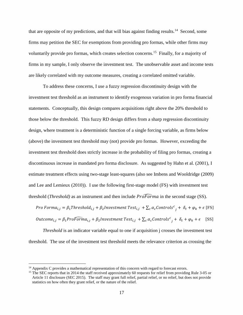
threshold (Threshold) as an instrument and then include 𝑃𝑟𝑜𝐹𝑜𝑟𝑚𝑎̂ in the second stage (SS).

𝑃𝑟𝑜 𝐹𝑜𝑟𝑚𝑎𝑖,𝑗 = 𝛽1𝑇ℎ𝑟𝑒𝑠ℎ𝑜𝑙𝑑𝑖,𝑗 + 𝛽2𝐼𝑛𝑣𝑒𝑠𝑡𝑚𝑒𝑛𝑡 𝑇𝑒𝑠𝑡𝑖,𝑗 + ∑ 𝛼𝑐𝐶𝑜𝑛𝑡𝑟𝑜𝑙𝑠𝑐𝑐 𝑗

+ 𝛿𝑡 + 𝜑𝑘 + 𝜖 [FS]

𝑂𝑢𝑡𝑐𝑜𝑚𝑒𝑖,𝑗 = 𝛽1𝑃𝑟𝑜𝐹𝑜𝑟𝑚𝑎𝑖,𝑗̂ + 𝛽2𝐼𝑛𝑣𝑒𝑠𝑡𝑚𝑒𝑛𝑡 𝑇𝑒𝑠𝑡𝑖,𝑗 + ∑ 𝛼𝑐𝐶𝑜𝑛𝑡𝑟𝑜𝑙𝑠𝑐

𝑐 𝑗+ 𝛿𝑡 + 𝜑𝑘 + 𝜖 [SS]

Threshold is an indicator variable equal to one if acquisition j crosses the investment test

threshold. The use of the investment test threshold meets the relevance criterion as crossing the

14 Appendix C provides a mathematical representation of this concern with regard to forecast errors. 15 The SEC reports that in 2014 the staff received approximately 60 requests for relief from providing Rule 3-05 or

Article 11 disclosure (SEC 2015). The staff may grant full relief, partial relief, or no relief, but does not provide

statistics on how often they grant relief, or the nature of the relief.

18

threshold increases the probability of filing pro formas. The exclusion criterion requires that

barely exceeding the investment test threshold at 20% does not result in a discontinuous change

in analyst forecast errors or announcement returns, other than through the effect of pro forma

disclosure. For private and subsidiary targets, I can only calculate the investment test, and thus

the asset test and income test are included in the error term of the first-stage model. This raises

the concern that the error term in the first stage might be correlated with the investment test

threshold, which would violate the exclusion criterion. Formally stated, the investment test

threshold would not be a valid instrument if either of the following occurs:

𝑐𝑜𝑣(𝐼𝑛𝑣𝑒𝑠𝑡 𝑇𝑒𝑠𝑡 𝑇ℎ𝑟𝑒𝑠ℎ𝑜𝑙𝑑, 𝐴𝑠𝑠𝑒𝑡 𝑇𝑒𝑠𝑡 𝑇ℎ𝑟𝑒𝑠ℎ𝑜𝑙𝑑 |𝐼𝑛𝑣𝑒𝑠𝑡 𝑡𝑒𝑠𝑡) ≠ 0 [𝐸𝐶1]

𝑐𝑜𝑣(𝐼𝑛𝑣𝑒𝑠𝑡 𝑇𝑒𝑠𝑡 𝑇ℎ𝑟𝑒𝑠ℎ𝑜𝑙𝑑, 𝐼𝑛𝑐𝑜𝑚𝑒 𝑇𝑒𝑠𝑡 𝑇ℎ𝑟𝑒ℎ𝑠𝑜𝑙𝑑 |𝐼𝑛𝑣𝑒𝑠𝑡 𝑡𝑒𝑠𝑡) ≠ 0 [𝐸𝐶2]

Including the investment test percentage in the first-stage controls for a linear relation between

the excluded tests and the investment test. However, a non-linear relation between the

investment test and the excluded tests would violate the exclusion criterion.

IV. SAMPLE SELECTION AND DESCRIPTIVE STATISTICS

There is no commercially available database of pro forma financial statements, so I

obtain a sample of acquisitions from SDC platinum and then hand-collect pro forma financial

information from SEC filings. I start my sample in 2002 to avoid acquisitions accounted for

under the pooling-of-interest method and the anomalous share-based technology acquisitions

identified in Moeller et al. (2005).16 I identify 25,120 acquisitions in SDC platinum, completed

between January 1, 2002, and December 31, 2016, with a US publicly traded acquirer and SDC

deal value greater than $10 million. I include acquisitions of foreign and domestic public,

16 Starting the sample in 2002 alleviates concerns about analyst conflicts of interest during the 1990s which led to

congressional investigations, the global settlement, and new regulations (Bradshaw et al. 2017; Kadan et al. 2008).

19

private, and subsidiary targets. I match each acquirer to Compustat, CRSP, and IBES, which

reduces the sample to 12,140 observations. Following Chen (2019), I use the ratio of SDC deal

value to acquirer’s pre-acquisition assets from the most recently completed annual period as a

proxy for the investment test. I remove all acquisitions with an investment test ratio below 5% or

greater than 40%, which reduces the sample to 5,247. Given the importance of appropriately

identifying firms above and below the 20% threshold, I verify the purchase price for acquisitions

with a deal value between 15% and 25% of acquirer pre-acquisition assets. Since one of my

main outcome variables is analyst forecast errors, I remove observations with acquirers covered

by less than three analysts and without forecasts in all four pre and post-acquisition quarters. To

reduce confounding effects from other acquisitions, I remove acquisitions in which the acquirer

completes another transaction above 20% in either the 365 days before or after closing. Finally, I

remove acquisitions completed by REITs or Real estate firms subject to the guidance Regulation

S-X 3-14, which has different thresholds. My final sample is 3,080 observations.

For each of the 3,080 acquisitions, I determine whether the acquiring firm provides

Article 11 pro forma financial statements. I conduct a keyword search of 8-K, S-4, and proxy

statement filings to identify a sample of firms who reference pro forma financial statements.17 I

review every disclosure to ensure that the firm provides Article 11 pro formas. For all

observations without pro forma disclosure that are above the investment test threshold, I

manually search Edgar filings to ensure no disclosure. Ultimately, 1,128 firms provide Article

11 pro forma disclosure. Table 1 shows the sample:

[INSERT TABLE 1]

17 I search 8-K, S-4 and proxy statement filings with for the phrases "unaudited W/250 pro forma W/250 acquisition

/merger/combin*." I search 8-K filings in the 100 day post-acquisition period. I search S-4 and proxy statement

filings between the acquisition announcement and closing date.

20

For each observation with pro forma disclosure, I hand-collect key balance sheet, annual income

statement, and footnote information. I remove 164 observations with confounding events, such

as a previous acquisition or disposition, or incomplete disclosure. I also remove 18 observations

with no target revenue, as I use purchase price to revenue as a test variable.

Descriptive Statistics

[INSERT TABLE 2 PANEL A]

Table 2 Panel A provides the number of acquisitions in 7 different investment test size

bins, using 5% intervals. For each bin, I present the number of observations, the percentage of

firms filing pro formas, the change in forecast errors, and the abnormal announcement return. I

find 19.5% of observations below the threshold include pro formas, with the percentage

increasing from 14.3% in the smallest bucket (5% to 10%) to 29.6% in the 15% to 20% size

bucket. The importance of the threshold is observable in the data. The percentage of firms

providing pro formas jumps from 29.6% right below the threshold, to 91.8% in the bucket right

above the threshold (20 to 25%). Overall, 94.6% of firms above the 20% threshold file pro

formas. I use the 20% threshold as an instrument, as crossing the threshold increases the

probability of providing pro formas. Figure 1 provides a graphical illustration of the

discontinuous increase in pro formas around the threshold.

[INSERT FIGURE 1]

The bottom of Table 2 Panel A shows that the average change in forecast errors is 5.0%

below the 20% threshold and 5.1% above the threshold. In particular, the change in forecast

errors falls to almost zero in the bin right above the threshold, and the average forecast error is

smaller in the 25-30% bin than in the 10-15%. Examining announcement returns, the average

return below the threshold is 1.0%, while the average return above the threshold is 1.9%.

21

A concern with using known thresholds as a source of exogenous variation is the

possibility of manipulation around the threshold. For example, Li et al. (2018) show that

acquiring firms alter the mix of cash and stock consideration, but not the amount of total

consideration, to avoid shareholder votes. To manipulate the investment test, the acquiring firm

shareholders must convince the target firm shareholders to accept a lower purchase price. Given

an average price of $665 million, an acquirer must convince target shareholders to accept $13.3

million less to manipulate the investment test from 21% to 19%. However, there is anecdotal

evidence of acquirers trying to avoid providing pro formas (Chen 2019), so I formally test

whether manipulation is of concern in my setting.

Starting with McCrary (2008), economists have developed tests to examine whether there

is a manipulation around a threshold. The general idea behind these tests is to examine whether

there is an abnormal number of observations right above or below the threshold, which would

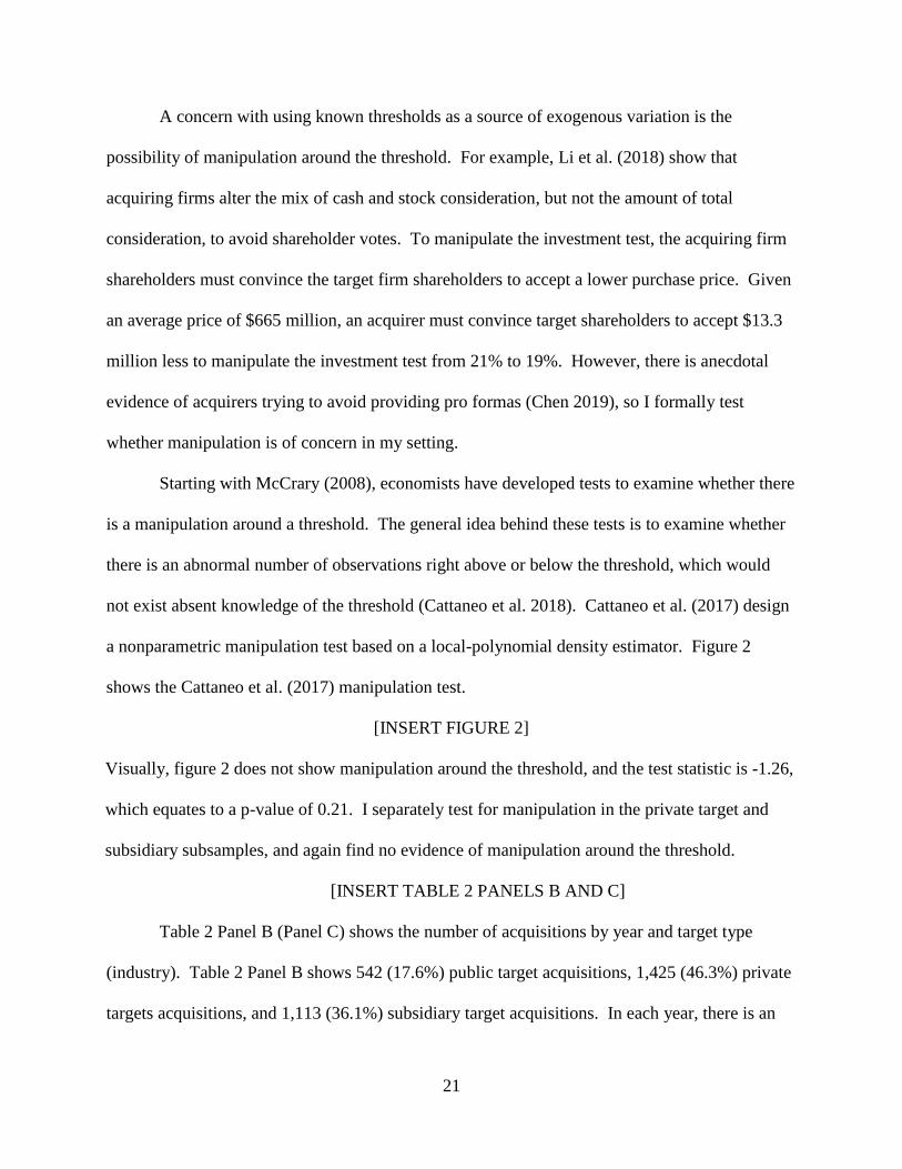
not exist absent knowledge of the threshold (Cattaneo et al. 2018). Cattaneo et al. (2017) design

a nonparametric manipulation test based on a local-polynomial density estimator. Figure 2

shows the Cattaneo et al. (2017) manipulation test.

[INSERT FIGURE 2]

Visually, figure 2 does not show manipulation around the threshold, and the test statistic is -1.26,

which equates to a p-value of 0.21. I separately test for manipulation in the private target and

subsidiary subsamples, and again find no evidence of manipulation around the threshold.

[INSERT TABLE 2 PANELS B AND C]

Table 2 Panel B (Panel C) shows the number of acquisitions by year and target type

(industry). Table 2 Panel B shows 542 (17.6%) public target acquisitions, 1,425 (46.3%) private

targets acquisitions, and 1,113 (36.1%) subsidiary target acquisitions. In each year, there is an

22

increase in post-acquisition forecast errors and positive announcement returns. The probability

of filing pro formas conditional on being above (below) the investment test threshold is between

88.1% and 100% (14.9% and 28.7%) with no discernable yearly trends.

Table 2 Panel C shows variation in purchase price by industry, with utilities and

telecommunications having the largest acquisitions. All industries have an increase in post-

acquisition forecast errors, and every industry other than utilities has positive acquisition

announcement returns. In industries other than finance, firms under (above) the 20% investment

threshold file pro formas in less than 30% (more than 91%) of observations. In the finance

industry, 55.3% of acquisitions below the threshold still file pro forma financial statements.18

This suggests that using the investment test as an instrument is weakest in the finance industry,

and I ensure all results are robust to dropping financial acquisitions.

Table 3 Panel A provides acquisition-level descriptive statistics. The average change in

forecast errors is 5.0%, the average abnormal return is 1.2%, and 36.6% observations include pro

formas. In 21.6% of cases, the acquisition falls above the investment test threshold, and the

acquirer provides pro formas. In 13.0% of cases, the acquisition falls below the investment test

threshold, but I verify that the acquisition crosses either the asset or income test threshold, and

pro forma disclosure is required. Finally, in 2.1% of cases, the firm includes pro forma financial

statements, but hand-collected data from the disclosure does not show the acquisition exceeding

one of the three thresholds.19 The target is foreign in 18.5% of observations and in a different

industry in 28.7% of observations. 10.5 (8) analysts cover the average (median) acquirer.

18 This is likely due to the structure of bank acquisitions, as the acquiring bank assumes all assets and liabilities and

banks have high leverage, thus making it relatively more likely that the asset test is greater than 20%. 19 I use historical target information contained in pro formas to determine whether pro forma disclosure below the

investment test threshold is mandated or voluntary. My classification likely contains measurement error as the

test calculations are complicated with multiple exceptions (SEC FRM 2017).

23

Table 3 Panel B shows the Pearson correlation matrix. There is an insignificant 0.01

correlation between my main outcomes measures (post-acquisition forecast errors and abnormal

returns). There is a positive correlation of 0.04, significant at the 5% level, between Pro Forma

and the change in post-acquisition forecast errors, inconsistent with H1A. As discussed above,

this positive association is not surprising as the SEC requires pro formas for larger transactions,

where forecasting earnings is likely more difficult. Pro Forma and announcement returns have a

positive correlation of 0.06, significant at the 0.01 level, consistent with H2A and H2B.

Finally, Table 3 Panel C describes pro forma disclosure using hand-collected data. While

all pro formas contain an annual income statement, only 77.2% contain an interim income

statement, and only 89.9% contain a balance sheet.20 On average, pro formas contain 13.9 notes,

although the average pro forma note is only a few sentences. On a pro forma basis, 37.6% of

acquisitions are accretive to EPS, and 45.6% increase net income. The average (median)

purchase price to revenue multiple is 5.10 (2.02). In 39.2% of observations, there is a negative

pro forma operating margin, and conditional on having a positive operating margin, the average

pro forma operating margin is 18.0%. The bottom of Table 3 Panel C compares historical target

financial metrics to historical plus pro forma financial metrics to provide evidence on the

magnitude of pro forma adjustments. On average, target revenue only changes by 2.5%, and in

66.0% of observations, there are no pro forma adjustments to target revenue. However, the

change in target operating income and net income both exceed 100%. On average, firms

recognize downward pro forma adjustments to revenue, operating income, and net income,

which is not surprising due to the application of purchase accounting.

20 A pro forma balance sheet is not required if the acquirer has filed a balance sheet reflecting the acquisition in a 10-

K or 10-Q filing (SEC FRM 2017, Section 3220).

24

V. A TEST OF THE ACCURACY ENHANCEMENT HYPOTHESIS

The accuracy enhancement hypothesis predicts a negative association between pro forma

disclosure and post-acquisition forecast errors. To test H1A, I estimate Equation 1 with the

change in forecast errors as the dependent variable for each of the four post-acquisition quarters.

Table 4 presents the results.

[INSERT TABLE 4]

In column 1, I estimate Equation 1 using OLS and find an insignificant coefficient on Pro

Forma. Using a fuzzy RD design in column 2, I find a negative coefficient on Pro Forma IV,

significant at the 0.01 level. For brevity, I do not present the first-stage model, but

unsurprisingly the F-statistic from the first stage is 285.8, suggesting no concerns about a weak

instrument. In column 3, I weight observations by 1 minus the absolute value of the distance to

the threshold, which places greater weight on observations closer to the threshold, and I continue

to document a negative association, significant at the 0.01 level. In columns 4 and 5, I split the

sample by post-acquisition quarters, with the first two quarters in column 4 and the second two

quarters in column 5, to test whether the documented effect is stronger in the quarters

immediately after the acquisition. In both subsamples, the coefficient on Pro Forma IV is

negative and significant, and coefficient estimates are of similar magnitude.21 In column 6, I

only include observations within the 15 to 25% window, which reduces the sample size to 2,548

(a reduction of 79.3%), and the coefficient on Pro Forma IV remains negative but is insignificant

at the 0.10 level. The first stage F-Test is only 27.7, suggesting that the insignificant coefficient

might be related to the well documented weak instrument problem (Gow et al. 2016; Feir et al.

21 The fact that coefficient estimates do not attenuate in quarters 3 and 4 is of some concern, as one would expect the

effects of pro forma to attenuate as more post-acquisition consolidated financial information becomes available.

To address this concern, I re-run the analysis using quarters in the year after the acquisition (t+5 to t+8) and in

untabulated results, find insignificant coefficient estimates.

25

2016).22 In column 8, I include an interaction term for the investment test threshold and the

investment test, which allows for the slope on the forcing variable to change when crossing the

threshold (Wooldridge 2010, pg 958). Again, I find a negative association between post-

acquisition forecast errors and Pro Forma IV.

In Table 4, the coefficient magnitude on Pro Forma IV is between -0.109 and -0.129,

which translates to a 10.9% to 12.9% decrease in the forecast errors. The coefficient on

investment test suggests that for an acquisition right at the 20% threshold, there is an increase in

analyst forecast errors of 6.9% to 9.0% (0.344*0.2 = 6.9% and 0.450*0.2= 9.0%). Thus, for an

acquisition right above the threshold, there is no post-acquisition increase in forecast errors.

In my main test I focus on analyst forecast errors, while prior literature often uses both

forecast errors and dispersion as measures of uncertainty (Ramnath et al. 2008). Barron et al.

(1998) show how researchers can use analyst forecasts to measure total uncertainty as the sum of

idiosyncratic uncertainty (dispersion in forecasts) and common uncertainty (squared forecast

errors – dispersion/number of analysts). To examine the robustness of results to alternative

dependent variables, I use the Barron et al. (1998) Total Uncertainty, Common Uncertainty, and

Idiosyncratic Uncertainty measures to test the accuracy enhancement hypothesis. I predict that

pro formas reduce Total Uncertainty and Common Uncertainty, but do not forward a hypothesis

related to dispersion as analytical models show that analyst forecast dispersion depends on the

analysts’ private information and differential ability to interpret public information (Barron et al.

1998; Harris and Raviv 1993; Kandel and Pearson 1995). Table 5 presents the results.

[INSERT TABLE 5]

22 Feir et al. (2016) note that the first-stage F-test rule of thumb of 10 used to identify weak instruments is not

suitable for identifying weak instrument in a fuzzy RD setting.

26

Table 5 shows a negative effect of pro forma disclosure on Barron et al. (1998) Total

Uncertainty, significant at the 0.01 level, using unweighted (column 1) or distance-weighted

regressions (column 2). Column 3 restricts the sample to observations between 15 and 25%, and

the coefficient on Pro Forma IV remains negative, significant at the 0.10 level. To interpret

economic magnitude, I compare the column 1 Pro Forma IV coefficient (-.057) to an acquisition

at the 20% threshold (20%*0.22 = 0.0432) and find that pro formas offset the increase in overall

uncertainty. When the dependent variable is Common Uncertainty in columns 4 through 6, the

coefficient on Pro Forma IV is negative and significant at the 0.01 or 0.10. In columns 6-9, the

dependent variable is Idiosyncratic Uncertainty, and the coefficient Pro Forma IV is

indistinguishable from zero at the 0.10 level. Collectively, the evidence in Tables 4 and 5

suggest that pro formas reduce post-acquisition forecast errors, but do not affect dispersion.23

A Test of H1B - Benefits Conditional on Pre-Existing Information Environment

To test whether the forecasting benefit of pro formas depends on the information

environment, I split the sample by analyst following and target type (public, private, subsidiary).

Following Botosan (1997), I test whether the results in Table 4 (forecast accuracy) and Table 5

(total and common uncertainty) differ based on the acquirer’s analyst following. Prior literature

shows that analysts both interpret public information and create new information (Asquith et al.

2005; Ivković and Jegadeesh 2004), which raises the possibility that analysts can produce the

information contained in pro formas absent mandated disclosure. Table 6 presents the results.

[INSERT TABLE 6]

23 The analysis in Tables 4 and 5 rely on plausibly exogenous variation in the mandatory requirement to provide pro

formas, but do not tie characteristics of pro forma disclosure to forecast errors. In the online appendix Table A1, I

show that analyst forecast errors are larger when pro forma earnings are less predictive of future earnings.

27

The top (bottom) panel presents results for acquirers with below (above) median analyst

following. For each outcome measure (AFE Change in columns 1-3, Total Uncertainty in

columns 4-6, and Common Uncertainty in columns 7-9), I present results using an unweighted

regression, distance-weighted regression, and using the 15-25% window. In eight of the nine

columns in the top panel (low analyst following), the coefficient on Pro Forma IV is negative

and significant at the 0.01 or 0.10 level. Statistical significance is similar to Tables 4 and 5, even

though the sample is half the size. In the bottom panel (high analyst following), the coefficient

on Pro Forma IV is indistinguishable from zero in all 9 columns. These results suggest that pro

formas benefit firms with low analyst following. For firms with high analyst following, it

appears that the information contained in pro formas is produced even absent a mandate.

Next, I conduct subsample analysis by target type as pre-acquisition information and

potential benefits to disclosure may differ for public, private, and subsidiary targets. For

example, it might be more difficult to forecast post-acquisition earnings for private targets

without historical financial statements or analyst coverage. For subsidiary and private targets, I

continue to use the investment test threshold as my instrument. For public targets, I observe all

three tests and use the three thresholds as instruments. Table 7 presents the results.

[INSERT TABLE 7]

For the subsample of private (subsidiary) targets, columns 1 through 3 (4 through 6)

show the coefficient on Pro Forma IV is negative and significant at the 0.05 (0.10) level. For

public targets, the coefficient on Pro Forma IV is negative in column 7 but insignificant at

conventional levels. The smaller subsample of public targets weakens my test, but observing all

three thresholds increases the strength of my instrument (the first stage F test is 303.4, higher

than the first stage F of 160.9 or 84.6 for private and subsidiary targets, respectively). In column

28

8 (column 9), when the dependent variable is total uncertainty (common uncertainty), the

coefficient on Pro Forma IV is negative and significant at the 0.10 level.

Overall, I interpret the results Tables 4 through 7 as evidence consistent with the

accuracy enhancement hypothesis. Using a fuzzy RD design, I find that pro formas reduce

forecast errors, total uncertainty, and common uncertainty. The benefits to pro forma disclosure

appear concentrated in firms with a weaker pre-existing information environment. In the online

appendix (Table A2), I show that results are robust to measuring outcomes using percentile ranks

(Panel A), excluding acquirers hiring an investment bank which may create conflicts of interests

(Panel B), including high order polynomials of the forcing variable (Panel C), and removing

observations close to the threshold possibly subject to manipulation (Panel D).

VI. A TEST OF THE INCENTIVE ALIGNMENT HYPOTHESIS

The incentive alignment hypothesis predicts that pro formas are useful in mitigating an

agency problem by providing information about target quality. To test H2A and H2B, I first

examine whether information in pro forma financial statements explains variation in acquisition

returns (i.e., can be used to identify low-quality projects) by estimating the following equation

𝐴𝑅𝐸𝑇𝑖,𝑗 = 𝛽1𝑃𝐹 𝑉𝑎𝑟𝑠𝑖,𝑗 + ∑ 𝛼𝑐𝐶𝑜𝑛𝑡𝑟𝑜𝑙𝑠𝑐𝑐 𝑖,𝑗

+ 𝛿𝑡 + 𝜑𝑘 + 𝜖 [2]

Where PF Vars is either an indicator variable equal to 1 if the acquisition increases pro forma

EPS (Accretive EPS), or the decile rank of the purchase price to pro forma revenue (Price to

Revenue) and the decile rank of pro forma operating margin (PF Op Margin). While firms file

pro formas after the announcement date, many firms discuss the acquisition on a conference call

or in a press release (Kimbrough and Louis 2011). I include industry (𝜑𝑘) and year (𝛿𝑡) fixed

effects, and cluster standard errors by firm. Table 8 presents the results.

[INSERT TABLE 8]

29

Table 8 column 1 presents the results without any pro forma variables. Consistent with

prior literature (Golubov et al. 2012; Bao and Edmans 2011; Chen 2019), there are negative

coefficients on Public Tgt, Tobin Q, Size, and Serial Acq. The adjusted R2 of 5.3% is similar to

prior literature that documents an adjusted R2 between 3.6 and 6.0% using firm and deal

characteristics (Golubov et al. 2015). In column 2, I include EPS Accretive. The coefficient on

EPS Accretive is positive, significant at the 0.05 level, and suggests 1.1% higher announcement

returns on acquisitions that are accretive to pro forma EPS. In column 3, I include Price to

Revenue and PF Op Margin. The negative coefficient on Price to Revenue suggests a negative

market reaction when the acquirer pays more for target historical revenue, and the positive

coefficient on PF Op Margin suggests higher returns when pro forma operating margins are

higher. In column 3, the adjusted R2 increases to 7.6%, a relative increase of 43.4% compared to

column 1. Columns 1-3 include all acquisitions, even though traditional accounting metrics may

not explain some acquirer returns. For example, a biotechnology firm might purchase a target to

obtain in-process research and development (IPR&D), and the acquirers’ stock might not trade

based on accounting fundamentals. To address this concern, I repeat the analysis on the subset

of acquirers who either have a current, or 5-year average, unlevered PE ratio between zero and

50 (columns 4-6). In this smaller subsample, results are qualitatively similar.

Having established that pro formas provide a measure of target quality, I proceed to test

H2A and H2B. I predict a positive coefficient on Pro Forma if pro forma disclosure mitigates an

incentive alignment problem. Table 9 Panel A (Table 9 Panel B) presents results using value-

weighted (Market model, Fama-French 3-Factor, and a 4-factor model) abnormal returns.

[INSERT TABLE 9 PANELS A AND B]

30

In Table 9 Panel A, column 1 (column 2) presents results when adding Pro Forma (and the

investment test ratio) to the standard announcement return model. In both cases, the coefficient

on pro forma is positive, significant at the 0.01 or 0.05 level, and suggests 0.7% to 0.9% higher

returns when the acquirer provides pro formas. Since firms may voluntarily provide pro formas,

I split the Pro Forma variable into mandated and voluntary disclosure. While the coefficients on

both voluntary and mandatory pro forma are positive and similar in magnitude, only the

coefficient on PF Mandatory is significant at the 0.10 level. So far, the evidence is consistent

with both H2A and H2B. To provide evidence on the type of incentive alignment problem, I

split the sample by target type and whether the acquirer engages a 3rd party advisor.

For the acquisition of public targets, reputational incentives due to greater publicity might

mitigate any agency problem (Golubov et al. 2012). In column 4, I restrict the sample to public

targets and find the coefficient on PF Mandatory is indistinguishable from zero. Columns 5 and

6 split the sample non-public targets into those with no 3rd party advisor (column 5) and those

with a 3rd party advisor (column 6). In column 5 (column 6), the coefficient on PF Mandatory is

positive, significant at the 0.05 (0.01) level. In column 6 (private target acquisitions involving a

3rd party advisor), the coefficient magnitude suggests a 1.7% larger returns when pro forma

disclosure is required.

In columns 1-6, I use OLS to facilitate comparison with prior literature (Golubov et al.

2012; Chen 2019). However, unobservable acquisition characteristics might bias the pro forma

coefficient estimates. For example, pro formas are more likely when the target has high

historical earnings due to the income test, and Table 8 shows higher earnings are associated with

higher announcement returns, creating a correlated omitted variable. To address this concern, I

use a fuzzy RD design with the investment test as a threshold. Columns 7-9 presents the results.

31

In column 7 (public target subsample), the coefficient on the pro forma test variable is

insignificant at the 0.10 level, similar to column 4. Column 8 presents the results for the private

target sample without an 3rd party advisor. The coefficient on Pro Forma IV is indistinguishable

from zero, a change from column 5. In column 9, I continue to find a positive coefficient on the

pro forma variable in the subsample of non-public target acquisitions with outside advisors.

Table 9 Panel B shows similar inferences using three different return measures.

Conditioning on Analyst Following

Section 5 provides evidence that information contained within pro formas is produced

even without a mandate for acquirers with high analyst following and the forecasting benefit of

pro formas in concentrated in acquirers with low analyst following. Prior literature uses low

analyst following as a measure of high information asymmetry (Brennan and Subrahmanyam

1995; Armstrong et al. 2011) and shows incentive alignment problems are more pronounced

when there is high information asymmetry (Francis and Martin 2010). For these reasons, I split

the sample by analyst following and repeat the analysis in Table 9. Table 10 presents the results.

[INSERT TABLE 10]

The top (bottom) panel presents results for acquirers with below (above) median analyst

following. In columns 1 through 3, the coefficient on Pro Forma is positive and significant at

the 0.01 level in the low analyst subsample, and statistically indistinguishable from zero in the

high analyst subsample. In the low analyst subsample, the coefficient PF Mandatory (Pro

Forma IV) is positive and significant in columns 5 and 6 (column 9), consistent with Table 9

Panels A and B. In contrast, in the high analyst subsample, the coefficient on pro forma switch

from negative and significant (column 4) to positive and significant (column 6), and is otherwise

indistinguishable from zero (columns 5, 7, 8, and 9). Overall, Table 10 suggests the incentive

32

alignment benefit is concentrated in the subsample of acquirers with low analyst following, the

same subsample in which I find a forecasting benefit to Article 11 pro forma disclosure.

Additional Analysis

Collectively, the evidence points towards a positive association between pro forma

disclosure and target quality in acquisitions of non-public targets. Results differ based on

acquirer analyst following and the involvement of outside advisors. To provide evidence on the

characteristics of acquisitions involving an outside advisor, I estimate the following equation

𝑃𝐹 𝑉𝑎𝑟𝑠𝑖,𝑗 = 𝛽1𝐴𝑐𝑞 𝐴𝑑𝑣𝑖𝑠𝑜𝑟𝑖,𝑗 + ∑ 𝛼𝑐𝐶𝑜𝑛𝑡𝑟𝑜𝑙𝑠𝑐𝑐 𝑖,𝑗

+ 𝛿𝑡 + 𝜑𝑘 + 𝜖 [3]

Where PF Vars are the same three pro forma metrics from Equation 2 and Table 8, the test

variable is Acq Advisor, and I include controls and fixed effects. 24 Table 11 presents the results.

[INSERT TABLE 11]

Columns 1 and 2 (columns 3 and 4) present the results when the dependent variable is Accretive

EPS using a linear probability model (Logit). In all 4 columns, the coefficient on Acq Advisor is

negative and statistically significant. In column 1 (column 2), the 0.071 (0.067) magnitude

suggests acquisitions with an outside advisor are 7.1% (6.7%) less likely to be accretive to EPS

on a pro forma basis, an 18.9% (17.8%) decrease compared to the unconditional mean of 37.6%.

Columns 5 and 6 show no association between outside advisor involvement and the revenue

multiple paid in the acquisition. Columns 7 and 8 show outside advisor involvement is

associated with lower pro forma operating margins; both coefficient estimates are significant at

the 0.01 level. Together, the results suggest that advisor-assisted acquisitions are less likely to

24 Unfortunately I can only conduct this analysis on the subsample of acquisitions with pro formas. If an incentive

alignment problem does exist and is mitigated by pro forma disclosure, then analysis on the subsample of

acquisitions with pro formas may find no remaining differences between advisor and non-advisor deals.

33

be accretive to pro forma EPS, not because the acquirer pays a higher multiple for revenue, but

instead because advisor-assisted acquisitions have lower operating margins.

I interpret the results in Tables 8 through 11 as follows. Pro forma disclosure contains

information that is useful in understanding the quality of target selection. Mandated pro forma

disclosure is also associated with higher acquisition returns, concentrated in acquisitions of non-

public targets with the use of a 3rd party advisors. This evidence is consistent with pro forma

disclosure alleviating an incentive alignment problem between shareholders and firm advisors.

VII. CONCLUSION

The purpose of, and benefits to, mandatory disclosure are widely debated and depend on

the nature of information production without a mandatory requirement (Stigler 1964; Coffee Jr

1984; Mahoney 2009; Dye 1990). In a sample of 3,080 acquisitions, I test whether mandated pro

forma disclosure reduces analyst forecast errors, as predicted by the accuracy enhancement

hypothesis, or alleviates an incentive alignment problem. Using a fuzzy RD design, I provide

evidence that mandated pro forma disclosure improves analysts’ forecast accuracy. I find a

reduction in forecast errors only for firms with below-median analyst following, suggesting that

the benefits to pro forma disclosure depend on the pre-existing information environment. Using

announcement returns as a measure of target quality, I document higher quality target selection

in acquisitions with pro forma disclosure, concentrated in acquisitions of non-public targets with

outside advisors. I interpret the evidence as mandated pro forma disclosure mitigating an

incentive alignment problem between outside advisors and shareholders by improving

transparency regarding target selection. My results make a contribution to the literature on

mandated disclosure (Leuz and Wysocki 2016) and provide evidence on an issue important to

the SEC’s project on disclosure effectiveness (SEC 2015).

34

REFERENCES

Admati, A. R., and P. Pfleiderer. 2000. Forcing firms to talk: Financial disclosure regulation and

externalities. The Review of Financial Studies 13 (3):479-519.

Andrade, G., M. Mitchell, and E. Stafford. 2001. New evidence and perspectives on mergers.

Journal of economic perspectives 15 (2):103-120.

Armstrong, C. S., J. E. Core, D. J. Taylor, and R. E. Verrecchia. 2011. When does information

asymmetry affect the cost of capital? Journal of Accounting Research 49 (1):1-40.

Asquith, P., M. B. Mikhail, and A. S. Au. 2005. Information content of equity analyst reports.

Journal of Financial Economics 75 (2):245-282.

AT&T. 2015. AT&T Unaudited Pro Forma Condensed Combined Financial Statements.

Bao, J., and A. Edmans. 2011. Do investment banks matter for M&A returns? The Review of

Financial Studies 24 (7):2286-2315.

Barron, O. E., O. Kim, S. C. Lim, and D. E. Stevens. 1998. Using analysts' forecasts to measure

properties of analysts' information environment. Accounting Review:421-433.

Barth, M. E., W. H. Beaver, and W. R. Landsman. 2001. The relevance of the value relevance

literature for financial accounting standard setting: another view. Journal of Accounting

and Economics 31 (1-3):77-104.

Benston, G. J. 1969. The value of the SEC's accounting disclosure requirements. The Accounting

Review 44 (3):515-532.

———. 1973. Required disclosure and the stock market: An evaluation of the Securities

Exchange Act of 1934. The American Economic Review 63 (1):132-155.

Berger, P. G. 2011. Challenges and opportunities in disclosure research—A discussion of ‘the

financial reporting environment: Review of the recent literature’. Journal of Accounting

and Economics 51 (1-2):204-218.

Betton, S., B. E. Eckbo, and K. S. Thorburn. 2008. Corporate takeovers. Handbook of Corporate

Finance: Empirical Corporate Finance 2:291-430.

Beyer, A., D. A. Cohen, T. Z. Lys, and B. R. Walther. 2010. The financial reporting

environment: Review of the recent literature. Journal of Accounting and Economics 50

(2):296-343.

Botosan, C. A. 1997. Disclosure level and the cost of equity capital. Accounting Review:323-349.

Bowers, H., and W. R. Latham. 2006. Information asymmetry, litigation risk, uncertainty and the

demand for fairness opinions: Evidence from US mergers and acquisitions, 1980-2002.

Working Paper.

Bowers, H. M. 2001. Fairness opinions and the business judgment rule: an empirical

investigation of target firms' use of fairness opinions. Nw. UL Rev. 96:567.

Bradshaw, M., Y. Ertimur, and P. O'Brien. 2017. Financial analysts and their contribution to

well-functioning capital markets. Foundations and Trends® in Accounting 11 (3):119-

191.

Bradshaw, M. T., T. E. Christensen, K. H. Gee, and B. C. Whipple. 2018. Analysts’ GAAP

earnings forecasts and their implications for accounting research. Journal of Accounting

and Economics 66 (1):46-66.

Brennan, M. J., and A. Subrahmanyam. 1995. Investment analysis and price formation in

securities markets. Journal of Financial Economics 38 (3):361-381.

Buffett, W. 2018. Berkshire Hathaway 2017 Annual Shareholder Letter.

35

Bushee, B. J., and C. Leuz. 2005. Economic consequences of SEC disclosure regulation:

evidence from the OTC bulletin board. Journal of Accounting and Economics 39 (2):233-

264.

Bushman, R., E. Engel, and A. Smith. 2006. An analysis of the relation between the stewardship

and valuation roles of earnings. Journal of Accounting Research 44 (1):53-83.

Cattaneo, M. D., M. Jansson, and X. Ma. 2017. Simple Local Polynomial Density Estimators.

———. 2018. Manipulation testing based on density discontinuity. The Stata Journal 18

(1):234-261.

Chang, S. 1998. Takeovers of privately held targets, methods of payment, and bidder returns.

The Journal of Finance 53 (2):773-784.

Chemmanur, T. J., and P. Fulghieri. 1994. Investment bank reputation, information production,

and financial intermediation. The Journal of Finance 49 (1):57-79.

Chen, C. W. 2019. The disciplinary role of financial statements: evidence from mergers and

acquisitions of privately held targets. Journal of Accounting Research.

Christensen, H. B., L. Hail, and C. Leuz. 2013. Mandatory IFRS reporting and changes in

enforcement. Journal of Accounting and Economics 56 (2):147-177.

Coffee Jr, J. C. 1984. Market failure and the economic case for a mandatory disclosure system.

Virginia Law Review:717-753.

Comment, R. t. S. R. f. Comments on Request for Comment on the Effectiveness of Financial

Disclosures about Entities Other than the Registrant 2015 [cited. Available from

https://www.sec.gov/comments/s7-20-15/s72015.shtml.

Deloitte. 2018. A Roadmap to SEC Reporting Considerations for Business Combinations. In

Roadmap Series.

Dye, R. A. 1990. Mandatory versus voluntary disclosures: The cases of financial and real

externalities. Accounting Review:1-24.

Easterbrook, F. H., and D. R. Fischel. 1996. The economic structure of corporate law: Harvard

University Press.

Erickson, M., S.-W. Wang, and X. F. Zhang. 2012. The change in information uncertainty and

acquirer wealth losses. Review of Accounting Studies 17 (4):913-943.

FASB. 2010. Conceptual Framework for Financial Reporting. Statement of Financial

Accounting Concepts No. 8: FASB Norwalk, CT.

Feir, D., T. Lemieux, and V. Marmer. 2016. Weak identification in fuzzy regression

discontinuity designs. Journal of Business & Economic Statistics 34 (2):185-196.

Francis, J. R., and X. Martin. 2010. Acquisition profitability and timely loss recognition. Journal

of Accounting and Economics 49 (1-2):161-178.

Francis, J. R., E. L. Maydew, and H. C. Sparks. 1999. The role of Big 6 auditors in the credible

reporting of accruals. Auditing: A Journal of Practice & Theory 18 (2):17-34.

Franck, T. Bank of America upgrades AT&T on Time Warner merger, sees little risk deal

overturned 2018 [cited 5/21/2019. Available from

https://www.cnbc.com/2018/07/30/att-upgraded-at-bank-of-america-time-warner-tax-

cuts-buoy-

outlook.html?__source=yahoo%7Cfinance%7Cheadline%7Cstory%7C&par=yahoo&yptr

=yahoo.

Friend, I., and E. S. Herman. 1964. The SEC through a glass darkly. The Journal of Business 37

(4):382-405.

36

Gigler, F., and T. Hemmer. 1998. On the frequency, quality, and informational role of mandatory

financial reports. Journal of Accounting Research 36:117-147.

Gjesdal, F. 1981. Accounting for stewardship. Journal of Accounting Research 19 (1):208-231.

Golubov, A., D. Petmezas, and N. G. Travlos. 2012. When it pays to pay your investment

banker: New evidence on the role of financial advisors in M&As. The Journal of Finance

67 (1):271-311.

Golubov, A., A. Yawson, and H. Zhang. 2015. Extraordinary acquirers. Journal of Financial

Economics 116 (2):314-330.

Gow, I. D., D. F. Larcker, and P. C. Reiss. 2016. Causal inference in accounting research.

Journal of Accounting Research 54 (2):477-523.

Graham, J. R., and C. R. Harvey. 2001. The theory and practice of corporate finance: Evidence

from the field. Journal of Financial Economics 60 (2-3):187-243.

Greenstone, M., P. Oyer, and A. Vissing-Jorgensen. 2006. Mandated disclosure, stock returns,

and the 1964 Securities Acts amendments. The Quarterly Journal of Economics 121

(2):399-460.

Grossman, S. J. 1981. The informational role of warranties and private disclosure about product

quality. The Journal of Law and Economics 24 (3):461-483.

Grossman, S. J., and O. D. Hart. 1980. Disclosure laws and takeover bids. The Journal of

Finance 35 (2):323-334.

Grossman, S. J., and J. E. Stiglitz. 1980. On the impossibility of informationally efficient

markets. The American Economic Review 70 (3):393-408.

Hahn, J., P. Todd, and W. Van der Klaauw. 2001. Identification and estimation of treatment

effects with a regression‐discontinuity design. Econometrica 69 (1):201-209.

Harris, M., and A. Raviv. 1993. Differences of opinion make a horse race. The Review of

Financial Studies 6 (3):473-506.

Haw, I.-M., K. Jung, and W. Ruland. 1994. The accuracy of financial analysts' forecasts after

mergers. Journal of Accounting, Auditing & Finance 9 (3):465-483.

Healy, P. M., and K. G. Palepu. 2001. Information asymmetry, corporate disclosure, and the

capital markets: A review of the empirical disclosure literature. Journal of Accounting

and Economics 31 (1-3):405-440.

Imbens, G. W., and J. M. Wooldridge. 2009. Recent developments in the econometrics of

program evaluation. Journal of economic literature 47 (1):5-86.

Institute, C. 2016. Re: File No. S7-20-15, Request for Comment on the Effectiveness of

Financial Disclosures About Entities Other Than the Registrant – Regulation S-X.

Ivković, Z., and N. Jegadeesh. 2004. The timing and value of forecast and recommendation

revisions. Journal of Financial Economics 73 (3):433-463.

Jarrell, G. A., and M. Bradley. 1980. The economic effects of federal and state regulations of

cash tender offers. The Journal of Law and Economics 23 (2):371-407.

Jensen, M. C. 1986. Agency costs of free cash flow, corporate finance, and takeovers. The

American Economic Review 76 (2):323-329.

Kadan, O., L. Madureira, R. Wang, and T. Zach. 2008. Conflicts of interest and stock

recommendations: The effects of the global settlement and related regulations. The

Review of Financial Studies 22 (10):4189-4217.

Kandel, E., and N. D. Pearson. 1995. Differential interpretation of public signals and trade in

speculative markets. Journal of Political Economy 103 (4):831-872.

37

Kanodia, C., and D. Lee. 1998. Investment and disclosure: The disciplinary role of periodic

performance reports. Journal of Accounting Research 36 (1):33-55.

Kimbrough, M. D., and H. Louis. 2011. Voluntary disclosure to influence investor reactions to

merger announcements: An examination of conference calls. The Accounting Review 86

(2):637-667.

Kisgen, D. J., and W. Song. 2009. Are fairness opinions fair? The case of mergers and

acquisitions. Journal of Financial Economics 91 (2):179-207.

Kosnik, R. D., and D. L. Shapiro. 1997. Agency conflicts between investment banks and

corporate clients in merger and acquisition transactions: Causes and remedies. Academy

of Management Perspectives 11 (1):7-20.

Kothari, S., K. Ramanna, and D. J. Skinner. 2010. Implications for GAAP from an analysis of

positive research in accounting. Journal of Accounting and Economics 50 (2):246-286.

Kothari, S. P., E. So, and R. Verdi. 2016. Analysts’ forecasts and asset pricing: A survey. Annual

Review of Financial Economics 8:197-219.

Lambert, R. A. 2001. Contracting theory and accounting. Journal of Accounting and Economics

32 (1):3-87.

Lee, D. S., and T. Lemieux. 2010. Regression discontinuity designs in economics. Journal of

economic literature 48 (2):281-355.

Leuz, C. 2018. Evidence-based policymaking: promise, challenges and opportunities for

accounting and financial markets research. Accounting and Business Research 48

(5):582-608.

Leuz, C., and P. D. Wysocki. 2016. The economics of disclosure and financial reporting

regulation: Evidence and suggestions for future research. Journal of Accounting Research

54 (2):525-622.

Li, K., T. Liu, and J. Wu. 2018. Vote avoidance and shareholder voting in mergers and

acquisitions. The Review of Financial Studies 31 (8):3176-3211.

Mahoney, P. G. 1995. Mandatory disclosure as a solution to agency problems. The University of

Chicago Law Review 62 (3):1047-1112.

———. 2009. The development of securities law in the United States. Journal of Accounting

Research 47 (2):325-347.

Masulis, R. W., C. Wang, and F. Xie. 2007. Corporate governance and acquirer returns. The

Journal of Finance 62 (4):1851-1889.

McCrary, J. 2008. Manipulation of the running variable in the regression discontinuity design: A

density test. Journal of econometrics 142 (2):698-714.

Moeller, S. B., F. P. Schlingemann, and R. M. Stulz. 2005. Wealth destruction on a massive

scale? A study of acquiring‐firm returns in the recent merger wave. The Journal of

Finance 60 (2):757-782.

Morck, R., A. Shleifer, and R. W. Vishny. 1990. Do managerial objectives drive bad

acquisitions? The Journal of Finance 45 (1):31-48.

Ohlson, J. A. 1995. Earnings, book values, and dividends in equity valuation. Contemporary

Accounting Research 11 (2):661-687.

Paul, J. M. 1992. On the efficiency of stock-based compensation. The Review of Financial

Studies 5 (3):471-502.

PwC. 2014. Business combinations and noncontrolling interests: Application of the U.S. GAAP

and IFRS Standards.

38

Ramnath, S., S. Rock, and P. Shane. 2008. The financial analyst forecasting literature: A

taxonomy with suggestions for further research. International Journal of Forecasting 24

(1):34-75.

Schipper, K., and R. Thompson. 1983. The impact of merger-related regulations on the

shareholders of acquiring firms. Journal of Accounting Research:184-221.

SEC. About the SEC: What We Do 2013 [cited 5/21/2019. Available from

https://www.sec.gov/Article/whatwedo.html.

———. 2015. Request for comment of the effectiveness of financial disclosures about entities

other than the registrant

———. 2017. Financial Reporting Manual.

———. 2019. Amendments to Financial Disclosures about Acquired and Disposed Businesses.

Seligman, J. 1983. The historical need for a mandatory corporate disclosure system. J. Corp. L.

9:1.

Shaffer, M. 2018. Truth and Bias in M&A Target Fairness Valuations: Appraising the

Appraisals. Working Paper.

Simon, C. J. 1989. The effect of the 1933 Securities Act on investor information and the

performance of new issues. The American Economic Review:295-318.

Stigler, G. J. 1964. Public regulation of the securities markets. The Journal of Business 37

(2):117-142.

———. 1971. The theory of economic regulation. The Bell Journal of Economics and

Management Science:3-21.

Teoh, S. H., and T. Wong. 1993. Perceived auditor quality and the earnings response coefficient.

Accounting Review:346-366.

Travlos, N. G. 1987. Corporate takeover bids, methods of payment, and bidding firms' stock

returns. The Journal of Finance 42 (4):943-963.

Verrecchia, R. E. 1983. Discretionary disclosure. Journal of Accounting and Economics 5:179-

194.

———. 2001. Essays on disclosure. Journal of Accounting and Economics 32 (1-3):97-180.

Wooldridge, J. M. 2010. Econometric analysis of cross section and panel data: MIT press.

Young, E. 2016. SEC Financial Reporting Series: Pro forma financial information.

Young, E. a. 2019. To the Point: SEC proposes changing disclosure requirements for

acquisitions and disposals of businesses.

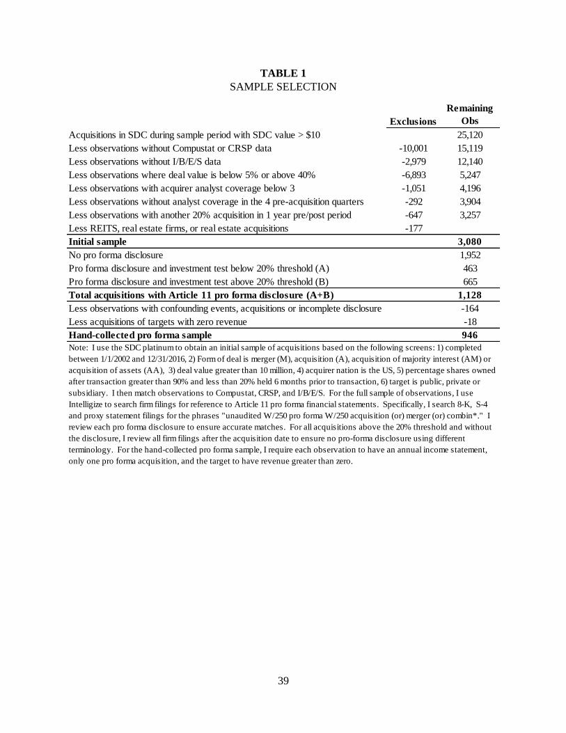
39

TABLE 1

SAMPLE SELECTION

Exclusions

Remaining

Obs

25,120

Less observations without Compustat or CRSP data -10,001 15,119

Less observations without I/B/E/S data -2,979 12,140

Less observations where deal value is below 5% or above 40% -6,893 5,247

Less observations with acquirer analyst coverage below 3 -1,051 4,196

Less observations without analyst coverage in the 4 pre-acquisition quarters -292 3,904

Less observations with another 20% acquisition in 1 year pre/post period -647 3,257

Less REITS, real estate firms, or real estate acquisitions -177

Initial sample 3,080

No pro forma disclosure 1,952

Pro forma disclosure and investment test below 20% threshold (A) 463

Pro forma disclosure and investment test above 20% threshold (B) 665

Total acquisitions with Article 11 pro forma disclosure (A+B) 1,128

Less observations with confounding events, acquisitions or incomplete disclosure -164

Less acquisitions of targets with zero revenue -18

Hand-collected pro forma sample 946

Acquisitions in SDC during sample period with SDC value > $10

Note: I use the SDC platinum to obtain an initial sample of acquisitions based on the following screens: 1) completed

between 1/1/2002 and 12/31/2016, 2) Form of deal is merger (M), acquisition (A), acquisition of majority interest (AM) or

acquisition of assets (AA), 3) deal value greater than 10 million, 4) acquirer nation is the US, 5) percentage shares owned

after transaction greater than 90% and less than 20% held 6 months prior to transaction, 6) target is public, private or

subsidiary. I then match observations to Compustat, CRSP, and I/B/E/S. For the full sample of observations, I use

Intelligize to search firm filings for reference to Article 11 pro forma financial statements. Specifically, I search 8-K, S-4

and proxy statement filings for the phrases "unaudited W/250 pro forma W/250 acquisition (or) merger (or) combin*." I

review each pro forma disclosure to ensure accurate matches. For all acquisitions above the 20% threshold and without

the disclosure, I review all firm filings after the acquisition date to ensure no pro-forma disclosure using different

terminology. For the hand-collected pro forma sample, I require each observation to have an annual income statement,

only one pro forma acquisition, and the target to have revenue greater than zero.

40

TABLE 2 PANEL A

DESCRIPTIVE STATISTICS BY INVESTMENT TEST SIZE

Investment Test Obs % Obs

Pro Forma

% AFE Change ARET

5% < Investment Test < 10% 1,247 40.5% 14.3% 3.5% 1.0%

10% ≤ Investment Test < 15% 715 23.2% 23.1% 7.3% 1.1%

15% ≤ Investment Test < 20% 415 13.5% 29.6% 5.7% 0.6%

20% ≤ Investment Test < 25% 219 7.1% 91.8% 0.2% 1.4%

25% ≤ Investment Test < 30% 192 6.2% 96.4% 6.4% 2.0%

30% ≤ Investment Test < 35% 159 5.2% 96.2% 8.1% 2.1%

35% ≤ Investment Test < 40% 133 4.3% 94.7% 7.9% 2.2%

Total / Average 3,080 100% 36.8% 5.0% 1.2%

Below Investment Test threshold 2,377 77.2% 19.5% 5.0% 1.0%

Above Investment Test threshold 703 22.8% 94.6% 5.1% 1.9%

Difference 75.1% 0.1% 0.9%

Difference - narrow subsample 62.1% -5.5% 0.8%

Note: The sample selection procedure is described in Table 1. This table presents the number of observations, percentage

of observations with pro forma financial statements, the average change in post-acquisition forecast errors, and abnormal

announcement date returns for 7 different size bins based on the investment test. I calculate the investment test as

purchase price scaled by acquirer assets from the most recent fiscal year, consistent with the requirements in S-X Rule 1-

02(w) and Article 11. For any investment test ratio within 5% of the threshold (i.e. 15 to 25%), I verify the purchase price

to ensure accurate calculate of the investment test ratio. For acquisitions below the 20% threshold, pro forma disclosure

may still be required if the acquisition exceeds either the asset or income test, which are unobservable for private and

subsidiary transactions, or the acquirer may voluntarily provide pro forma disclosure. For acquisition above the threshold,

firms may petition the SEC for relief from pro forma disclosure, explaining why the percentage is less than 100%.

41

TABLE 2 PANEL B

DESCRIPTIVE STATISTICS AND TARGET TYPE BY YEAR

Year Public Private Subsidiary

2002 37 96 91 $217 $90 24.3% 100.0% 75.7% 3.3% 1.1%

2003 43 80 65 $281 $100 28.7% 95.6% 66.9% 5.8% 2.1%

2004 49 120 70 $838 $117 19.7% 98.0% 78.4% 4.4% 0.9%

2005 38 108 85 $549 $100 19.7% 98.1% 78.5% 8.3% 1.0%

2006 42 109 80 $818 $128 20.6% 95.1% 74.5% 0.5% 1.3%

2007 61 112 65 $538 $155 22.5% 88.2% 65.8% 7.0% 0.5%

2008 30 109 58 $487 $112 17.2% 91.3% 74.1% 9.7% 0.9%

2009 20 50 37 $363 $110 14.9% 100.0% 85.1% 2.3% 1.1%

2010 38 72 65 $1,069 $202 16.5% 88.1% 71.6% 3.2% 0.8%

2011 23 102 70 $633 $164 17.6% 95.2% 77.6% 0.1% 0.9%

2012 28 104 93 $740 $175 16.2% 97.8% 81.6% 7.7% 1.3%

2013 34 81 84 $555 $158 24.2% 95.7% 71.5% 4.4% 1.5%

2014 35 114 90 $486 $199 18.8% 91.4% 72.6% 8.6% 1.5%

2015 36 91 71 $1,333 $222 17.5% 96.4% 78.9% 4.8% 1.5%

2016 28 77 89 $1,027 $225 14.9% 90.0% 75.1% 3.0% 1.5%

Total/Ave 542 1,425 1,113 $665 $142 19.5% 94.6% 75.1% 5.0% 1.2%

Note: The sample selection procedure is described in Table 1. This table presents the number of observations per year for each target type (subsidiary, private,

public). The column Pr(PF | Below Threshold) presents the probability of pro forma disclosure conditional on the acquisition being below the investment test

threshold. The column Pr(PF | Above Threshold) presents the probability of pro forma disclosure conditional on the acquisition being above the investment test

threshold. Threshold Jump is the difference between Pr(PF | Above Threshold) and Pr(PF | Below Threshold). Average AFE change presents the average change in

analysts forecast errors (AFE) in the 4 post-acquisition quarters, compared the 4 pre-acquisition quarters, scaled by pre-acquisition average EPS. Abnormal

announcement returns are measured in measured in the 3-day window (-1,0,1) centered on the acquisition announcement date. Following Bao and Edmans (2011), I

compute the abnormal return as the acquirer's CAR over the CRSP value weighted index.

ARET

Target Type AFE

Change

Pr(PF | Below

Threshold)

Pr(PF | Above

Threshold)

Threshold

Jump

Average

Purchase

Price

Median

Purchase

Price

42

TABLE 2 PANEL C

DESCRIPTIVE STATISTICS BY INDUSTRY

Indsutry Classification Obs

FF 1 - Consumer NonDurables - Food, Textiles, Apparel, Toys 165 $695 $210 14.8% 91.9% 77.0% 2.9% 2.8%

FF2 - Consumer Durables - Cars, TV's, Furniture, Appliances 59 $276 $143 4.5% 100.0% 95.5% 0.7% 1.2%

FF 3 - Manufacturing - Machinery, Trucks, Planes, Furniture 395 $471 $172 10.6% 95.3% 84.6% 3.2% 1.8%

FF 4 - Oil, Gas, and Coal Extraction and Products 197 $1,277 $231 23.5% 93.8% 70.3% 9.1% 1.2%

FF 5 - Chemicals and Allied Products 58 $628 $322 18.2% 100.0% 81.8% 1.1% 1.0%

FF 6 - Business Equipment - Computers, Software, Electronics 909 $437 $88 17.4% 94.8% 77.4% 6.4% 0.5%

FF 7 - Telephone and Television Transmission 87 $1,969 $250 19.4% 95.0% 75.6% 1.1% 0.6%

FF 8 - Utilities 48 $2,382 $889 27.3% 93.3% 66.1% 4.2% -0.6%

FF 9 -Wholesale, Retail, and Some Service (Laundries, Repair) 258 $465 $146 13.2% 98.1% 84.9% 2.0% 1.9%

FF 10 - Healthcare, Medical Equipment, and Drugs 285 $780 $123 14.8% 93.4% 78.6% 6.3% 0.8%

FF 11 - Finance 223 $1,401 $218 55.3% 93.9% 38.7% 2.6% 0.7%

FF 12 - Other -- Mines, Constr, Trans, Hotels, Serv, Entertain 396 $263 $105 19.7% 92.1% 72.4% 7.3% 1.8%

Total / Average 3,080 $665 $142 19.5% 94.6% 75.1% 5.0% 1.2%

AFE

Change ARET

Note: The sample selection procedure is described in Table 1. This table presents the number of observations per year for each Fama-French 12 industry. The column Pr(PF | Below

Threshold) presents the probability of pro forma disclosure conditional on the acquisition being below the investment test threshold. The column Pr(PF | Above Threshold) presents the

probability of pro forma disclosure conditional on the acquisition being above the investment test threshold. Threshold Jump is the difference between Pr(PF | Above Threshold) and Pr(PF

| Below Threshold). Average AFE change presents the average change in analysts forecast errors (AFE) in the 4 post-acquisition quarters, compared the 4 pre-acquisition quarters, scaled

by pre-acquisition average earnings. Abnormal announcement returns are measured in measured in the 3-day window (-1,0,1) centered on the acquisition announcement date. Following

Bao and Edmans (2011), I compute the abnormal return as the acquirer's CAR over the CRSP value weighted index.

Pr(PF|Below

Threshold)

Threshold

Jump

Pr(PF|Above

Threshold)

Average

Purchase

Price

Median

Purchase

Price

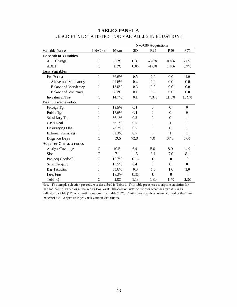
43

TABLE 3 PANEL A

DESCRIPTIVE STATISTICS FOR VARIABLES IN EQUATION 1

Variable Name Ind/Cont Mean SD P25 P50 P75

AFE Change C 5.0% 0.31 -3.8% 0.8% 7.6%

ARET C 1.2% 0.06 -1.8% 1.0% 3.9%

Pro Forma I 36.6% 0.5 0.0 0.0 1.0

Above and Mandatory I 21.6% 0.4 0.0 0.0 0.0

Below and Mandatory I 13.0% 0.3 0.0 0.0 0.0

Below and Voluntary I 2.1% 0.1 0.0 0.0 0.0

Investment Test C 14.7% 0.1 7.8% 11.9% 18.9%

Deal Characteristics

Foreign Tgt I 18.5% 0.4 0 0 0

Public Tgt I 17.6% 0.4 0 0 0

Subsidiary Tgt I 36.1% 0.5 0 0 1

Cash Deal I 56.1% 0.5 0 1 1

Diversifying Deal I 28.7% 0.5 0 0 1

External Financing I 51.3% 0.5 0 1 1

Diligence Days C 59.5 72.9 7.0 37.0 77.0

Acquirer Characteristics

Analyst Coverage C 10.5 6.9 5.0 8.0 14.0

Size C 7.1 1.5 6.1 7.0 8.1

Pre-acq Goodwill C 16.7% 0.16 0 0 0

Serial Acquirer I 15.5% 0.4 0 0 0

Big 4 Auditor I 89.6% 0.3 1.0 1.0 1.0

Loss Firm I 15.2% 0.36 0 0 0

Tobin Q C 2.03 1.13 1.30 1.70 2.38

Dependent Variables

Test Variables

Note: The sample selection procedure is described in Table 1. This table presents descriptive statistics for

test and control variables at the acquisition level. The column Ind/Cont shows whether a variable is an

indicator variable ("I") or a continuous/count variable ("C"). Continuous variables are winsorized at the 1 and

99 percentile. Appendix B provides variable definitions.

N=3,080 Acquisitions

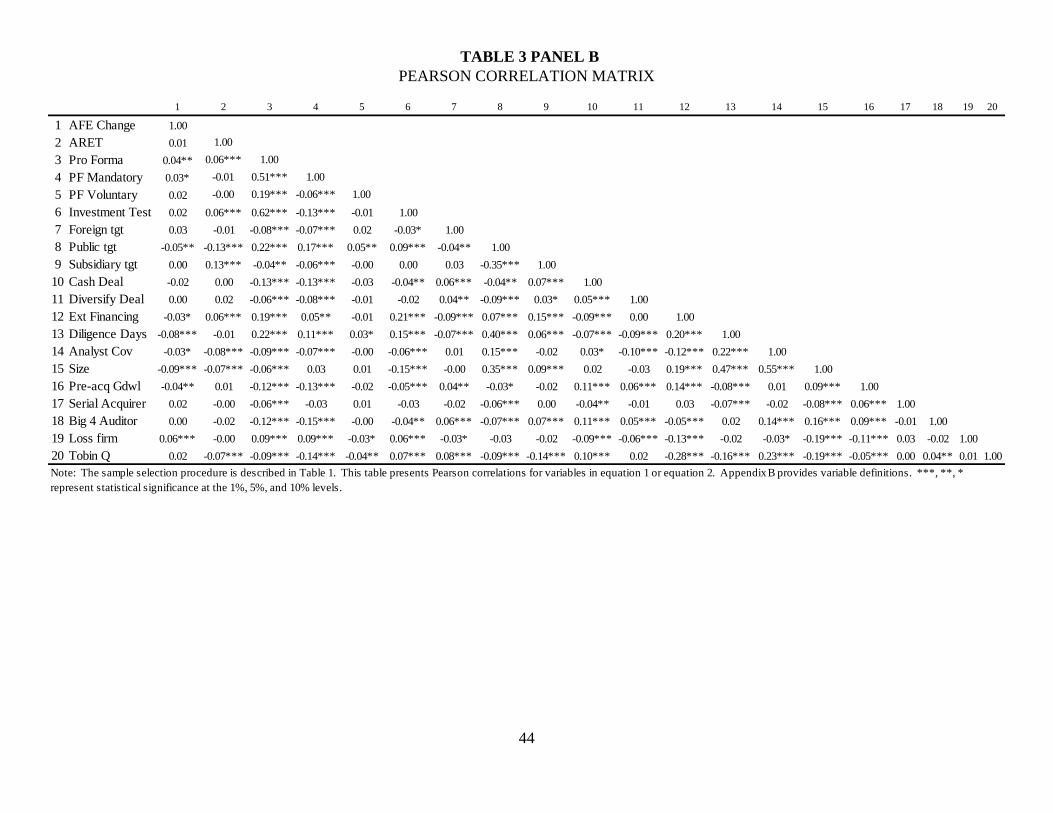
44

TABLE 3 PANEL B

PEARSON CORRELATION MATRIX

1 2 3 4 5 6 7 8 9 10 11 12 13 14 15 16 17 18 19 20

1 AFE Change 1.00

2 ARET 0.01 1.00

3 Pro Forma 0.04** 0.06*** 1.00

4 PF Mandatory 0.03* -0.01 0.51*** 1.00

5 PF Voluntary 0.02 -0.00 0.19*** -0.06*** 1.00

6 Investment Test 0.02 0.06*** 0.62*** -0.13*** -0.01 1.00

7 Foreign tgt 0.03 -0.01 -0.08*** -0.07*** 0.02 -0.03* 1.00

8 Public tgt -0.05** -0.13*** 0.22*** 0.17*** 0.05** 0.09*** -0.04** 1.00

9 Subsidiary tgt 0.00 0.13*** -0.04** -0.06*** -0.00 0.00 0.03 -0.35*** 1.00

10 Cash Deal -0.02 0.00 -0.13*** -0.13*** -0.03 -0.04** 0.06*** -0.04** 0.07*** 1.00

11 Diversify Deal 0.00 0.02 -0.06*** -0.08*** -0.01 -0.02 0.04** -0.09*** 0.03* 0.05*** 1.00

12 Ext Financing -0.03* 0.06*** 0.19*** 0.05** -0.01 0.21*** -0.09*** 0.07*** 0.15*** -0.09*** 0.00 1.00

13 Diligence Days -0.08*** -0.01 0.22*** 0.11*** 0.03* 0.15*** -0.07*** 0.40*** 0.06*** -0.07*** -0.09*** 0.20*** 1.00

14 Analyst Cov -0.03* -0.08*** -0.09*** -0.07*** -0.00 -0.06*** 0.01 0.15*** -0.02 0.03* -0.10*** -0.12*** 0.22*** 1.00

15 Size -0.09*** -0.07*** -0.06*** 0.03 0.01 -0.15*** -0.00 0.35*** 0.09*** 0.02 -0.03 0.19*** 0.47*** 0.55*** 1.00

16 Pre-acq Gdwl -0.04** 0.01 -0.12*** -0.13*** -0.02 -0.05*** 0.04** -0.03* -0.02 0.11*** 0.06*** 0.14*** -0.08*** 0.01 0.09*** 1.00

17 Serial Acquirer 0.02 -0.00 -0.06*** -0.03 0.01 -0.03 -0.02 -0.06*** 0.00 -0.04** -0.01 0.03 -0.07*** -0.02 -0.08*** 0.06*** 1.00

18 Big 4 Auditor 0.00 -0.02 -0.12*** -0.15*** -0.00 -0.04** 0.06*** -0.07*** 0.07*** 0.11*** 0.05*** -0.05*** 0.02 0.14*** 0.16*** 0.09*** -0.01 1.00

19 Loss firm 0.06*** -0.00 0.09*** 0.09*** -0.03* 0.06*** -0.03* -0.03 -0.02 -0.09*** -0.06*** -0.13*** -0.02 -0.03* -0.19*** -0.11*** 0.03 -0.02 1.00

20 Tobin Q 0.02 -0.07*** -0.09*** -0.14*** -0.04** 0.07*** 0.08*** -0.09*** -0.14*** 0.10*** 0.02 -0.28*** -0.16*** 0.23*** -0.19*** -0.05*** 0.00 0.04** 0.01 1.00

Note: The sample selection procedure is described in Table 1. This table presents Pearson correlations for variables in equation 1 or equation 2. Appendix B provides variable definitions. ***, **, *

represent statistical significance at the 1%, 5%, and 10% levels.

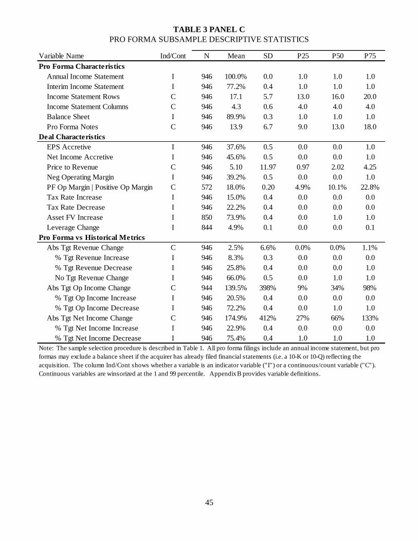
45

TABLE 3 PANEL C

PRO FORMA SUBSAMPLE DESCRIPTIVE STATISTICS

Variable Name Ind/Cont N Mean SD P25 P50 P75

Annual Income Statement I 946 100.0% 0.0 1.0 1.0 1.0

Interim Income Statement I 946 77.2% 0.4 1.0 1.0 1.0

Income Statement Rows C 946 17.1 5.7 13.0 16.0 20.0

Income Statement Columns C 946 4.3 0.6 4.0 4.0 4.0

Balance Sheet I 946 89.9% 0.3 1.0 1.0 1.0

Pro Forma Notes C 946 13.9 6.7 9.0 13.0 18.0

EPS Accretive I 946 37.6% 0.5 0.0 0.0 1.0

Net Income Accretive I 946 45.6% 0.5 0.0 0.0 1.0

Price to Revenue C 946 5.10 11.97 0.97 2.02 4.25

Neg Operating Margin I 946 39.2% 0.5 0.0 0.0 1.0

PF Op Margin | Positive Op Margin C 572 18.0% 0.20 4.9% 10.1% 22.8%

Tax Rate Increase I 946 15.0% 0.4 0.0 0.0 0.0

Tax Rate Decrease I 946 22.2% 0.4 0.0 0.0 0.0

Asset FV Increase I 850 73.9% 0.4 0.0 1.0 1.0

Leverage Change I 844 4.9% 0.1 0.0 0.0 0.1

Abs Tgt Revenue Change C 946 2.5% 6.6% 0.0% 0.0% 1.1%

% Tgt Revenue Increase I 946 8.3% 0.3 0.0 0.0 0.0

% Tgt Revenue Decrease I 946 25.8% 0.4 0.0 0.0 1.0

No Tgt Revenue Change I 946 66.0% 0.5 0.0 1.0 1.0

Abs Tgt Op Income Change C 944 139.5% 398% 9% 34% 98%

% Tgt Op Income Increase I 946 20.5% 0.4 0.0 0.0 0.0

% Tgt Op Income Decrease I 946 72.2% 0.4 0.0 1.0 1.0

Abs Tgt Net Income Change C 946 174.9% 412% 27% 66% 133%

% Tgt Net Income Increase I 946 22.9% 0.4 0.0 0.0 0.0

% Tgt Net Income Decrease I 946 75.4% 0.4 1.0 1.0 1.0

Note: The sample selection procedure is described in Table 1. All pro forma filings include an annual income statement, but pro

formas may exclude a balance sheet if the acquirer has already filed financial statements (i.e. a 10-K or 10-Q) reflecting the

acquisition. The column Ind/Cont shows whether a variable is an indicator variable ("I") or a continuous/count variable ("C").

Continuous variables are winsorized at the 1 and 99 percentile. Appendix B provides variable definitions.

Deal Characteristics

Pro Forma Characteristics

Pro Forma vs Historical Metrics

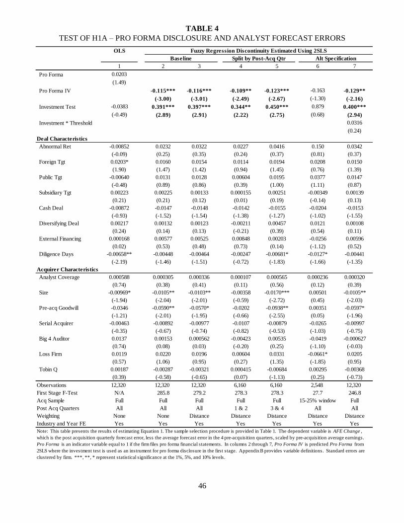
46

TABLE 4

TEST OF H1A – PRO FORMA DISCLOSURE AND ANALYST FORECAST ERRORS

OLS

1 2 3 4 5 6 7

Pro Forma 0.0203

(1.49)

Pro Forma IV -0.115*** -0.116*** -0.109** -0.123*** -0.163 -0.129**

(-3.00) (-3.01) (-2.49) (-2.67) (-1.30) (-2.16)

Investment Test -0.0383 0.391*** 0.397*** 0.344** 0.450*** 0.879 0.400***

(-0.49) (2.89) (2.91) (2.22) (2.75) (0.68) (2.94)

Investment * Threshold 0.0316

(0.24)

Deal Characteristics

Abnormal Ret -0.00852 0.0232 0.0322 0.0227 0.0416 0.150 0.0342

(-0.09) (0.25) (0.35) (0.24) (0.37) (0.81) (0.37)

Foreign Tgt 0.0203* 0.0160 0.0154 0.0114 0.0194 0.0208 0.0150

(1.90) (1.47) (1.42) (0.94) (1.45) (0.76) (1.39)

Public Tgt -0.00640 0.0131 0.0128 0.00604 0.0195 0.0377 0.0147

(-0.48) (0.89) (0.86) (0.39) (1.00) (1.11) (0.87)

Subsidiary Tgt 0.00223 0.00225 0.00133 0.000155 0.00251 -0.00349 0.00139

(0.21) (0.21) (0.12) (0.01) (0.19) (-0.14) (0.13)

Cash Deal -0.00872 -0.0147 -0.0148 -0.0142 -0.0155 -0.0204 -0.0153

(-0.93) (-1.52) (-1.54) (-1.38) (-1.27) (-1.02) (-1.55)

Diversifying Deal 0.00217 0.00132 0.00123 -0.00211 0.00457 0.0121 0.00108

(0.24) (0.14) (0.13) (-0.21) (0.39) (0.54) (0.11)

External Financing 0.000168 0.00577 0.00525 0.00848 0.00203 -0.0256 0.00596

(0.02) (0.53) (0.48) (0.73) (0.14) (-1.12) (0.52)

Diligence Days -0.00658** -0.00448 -0.00464 -0.00247 -0.00681* -0.0127* -0.00441

(-2.19) (-1.46) (-1.51) (-0.72) (-1.83) (-1.66) (-1.35)

Acquirer Characteristics

Analyst Coverage 0.000588 0.000305 0.000336 0.000107 0.000565 0.000236 0.000320

(0.74) (0.38) (0.41) (0.11) (0.56) (0.12) (0.39)

Size -0.00969* -0.0105** -0.0103** -0.00358 -0.0170*** 0.00501 -0.0105**

(-1.94) (-2.04) (-2.01) (-0.59) (-2.72) (0.45) (-2.03)

Pre-acq Goodwill -0.0346 -0.0590** -0.0570* -0.0202 -0.0938** 0.00351 -0.0597*

(-1.21) (-2.01) (-1.95) (-0.66) (-2.55) (0.05) (-1.96)

Serial Acquirer -0.00463 -0.00892 -0.00977 -0.0107 -0.00879 -0.0265 -0.00997

(-0.35) (-0.67) (-0.74) (-0.82) (-0.53) (-1.03) (-0.75)

Big 4 Auditor 0.0137 0.00153 0.000562 -0.00423 0.00535 -0.0419 -0.000627

(0.74) (0.08) (0.03) (-0.20) (0.25) (-1.10) (-0.03)

Loss Firm 0.0119 0.0220 0.0196 0.00604 0.0331 -0.0661* 0.0205

(0.57) (1.06) (0.95) (0.27) (1.35) (-1.85) (0.95)

Tobin Q 0.00187 -0.00287 -0.00321 0.000415 -0.00684 0.00295 -0.00368

(0.39) (-0.58) (-0.65) (0.07) (-1.13) (0.25) (-0.73)

Observations 12,320 12,320 12,320 6,160 6,160 2,548 12,320

First Stage F-Test N/A 285.8 279.2 278.3 278.3 27.7 246.8

Acq Sample Full Full Full Full Full 15-25% window Full

Post Acq Quarters All All All 1 & 2 3 & 4 All All

Weighting None None Distance Distance Distance Distance Distance

Industry and Year FE Yes Yes Yes Yes Yes Yes Yes

Note: This table presents the results of estimating Equation 1. The sample selection procedure is provided in Table 1. The dependent variable is AFE Change ,

which is the post acquisition quarterly forecast error, less the average forecast error in the 4 pre-acquisition quarters, scaled by pre-acquisition average earnings.

Pro Forma is an indicator variable equal to 1 if the firm files pro forma financial statements. In columns 2 through 7, Pro Forma IV is predicted Pro Forma from

2SLS where the investment test is used as an instrument for pro forma disclosure in the first stage. Appendix B provides variable definitions. Standard errors are

clustered by firm. ***, **, * represent statistical significance at the 1%, 5%, and 10% levels.

Fuzzy Regression Discontinuity Estimated Using 2SLS

Baseline Split by Post-Acq Qtr Alt Specification

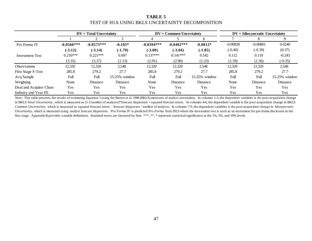
47

TABLE 5

TEST OF H1A USING BKLS UNCERTAINTY DECOMPOSITION

1 2 3 4 5 6 7 8 9

Pro Forma IV -0.0566*** -0.0575*** -0.105* -0.0394*** -0.0402*** -0.0812* -0.00828 -0.00801 0.0240

(-3.12) (-3.14) (-1.70) (-3.00) (-3.04) (-1.85) (-0.40) (-0.39) (0.37)

Investment Test 0.216*** 0.221*** 0.697 0.137*** 0.141*** 0.542 0.112 0.110 -0.243

(3.35) (3.37) (1.13) (2.91) (2.96) (1.23) (1.59) (1.56) (-0.35)

Observations 12,320 12,320 2,548 12,320 12,320 2,548 12,320 12,320 2,548

First Stage F-Test 285.8 279.2 27.7 285.8 279.2 27.7 285.8 279.2 27.7

Acq Sample Full Full 15-25% window Full Full 15-25% window Full Full 15-25% window

Weighting None Distance Distance None Distance Distance None Distance Distance

Deal and Acquirer Chars Yes Yes Yes Yes Yes Yes Yes Yes Yes

Industry and Year FE Yes Yes Yes Yes Yes Yes Yes Yes Yes

DV = Idiosyncratic Uncertainty

Note: This table presents the results of estimating Equation 1 using the Barron et al. 1998 (BKLS) measures of analyst uncertainty. In columns 1-3, the dependent variables is the post-acquisition change

in BKLS Total Uncertainty , which is measured as (1-1/number of analysts)*forecast dispersion + squared forecast errors. In columns 4-6, the dependent variable is the post-acquisition change in BKLS

Common Uncertainty, which is measured as squared forecast errors – forecast dispersion / number of analysts. In columns 7-9, the dependent variables is the post-acquisition change in Idiosyncratic

Uncertainty, which is measured using analyst forecast dispersion . Pro Forma IV is predicted Pro Forma from 2SLS where the investment test is used as an instrument for pro forma disclosure in the

first stage. Appendix B provides variable definitions. Standard errors are clustered by firm. ***, **, * represent statistical significance at the 1%, 5%, and 10% levels.

DV = Total Uncertainty DV = Common Uncertainty

48

TABLE 6

TEST OF H1B – ANALYSIS BASED ON ANALYST FOLLOWING

1 2 3 4 5 6 7 8 9

Pro Forma IV -0.165*** -0.169*** -0.412 -0.0932*** -0.0956*** -0.300* -0.0636*** -0.0652*** -0.197*

(-2.73) (-2.78) (-1.49) (-3.16) (-3.19) (-1.78) (-2.89) (-2.92) (-1.67)

Investment Test 0.507** 0.526** 3.250 0.302*** 0.312*** 2.584 0.192** 0.199** 1.668

(2.44) (2.50) (1.14) (3.02) (3.06) (1.49) (2.53) (2.57) (1.37)

Observations 6,224 6,224 1,384 6,224 6,224 1,384 6,224 6,224 1,384

First Stage F-Test 143.6 139.1 7.8 143.6 139.1 7.8 143.6 139.1 7.8

Pro Forma IV -0.0548 -0.0545 -0.00355 -0.00774 -0.00781 0.0520 -0.00721 -0.00763 0.00903

(-1.17) (-1.17) (-0.03) (-0.39) (-0.40) (1.12) (-0.53) (-0.57) (0.28)

Investment Test 0.212 0.210 -0.536 0.0619 0.0621 -0.698 0.0400 0.0418 -0.222

(1.24) (1.22) (-0.39) (0.82) (0.82) (-1.38) (0.78) (0.82) (-0.63)

Observations 6,096 6,096 1,164 6,096 6,096 1,164 6,096 6,096 1,164

First Stage F-Test 147.1 145.6 15.7 147.1 145.6 15.7 147.1 145.6 15.7

Acq Sample Full Full 15-25% window Full Full 15-25% window Full Full Full

Weighting None Distance Distance None None Distance Distance Distance Distance

Deal and Acquirer Chars Yes Yes Yes Yes Yes Yes Yes Yes Yes

Industry and Year FE Yes Yes Yes Yes Yes Yes Yes Yes Yes

Note: This table presents the results of estimating Equation 1 separately for below median analyst following (top panel) and above median analyst following (bottom panel). In columns 1-3,

the dependent variable is AFE Change , which is the post acquisition quarterly forecast error, less the average forecast error in the 4 pre-acquisition quarters, scaled by pre-acquisition

average earnings. In columns 4-6 (7-9) the dependent variables is the post-acquisition change in Total Uncertainty (Common Uncertainty ) from Barron et al. 1998 (see appendix B or Table

5 for calculation details). Pro Forma IV is predicted Pro Forma from 2SLS where the investment test is used as an instrument for pro forma disclosure in the first stage. Standard errors are

clustered by firm. ***, **, * represent statistical significance at the 1%, 5%, and 10% levels.

Below Median Analyst Following

Above Median Analyst Following

DV = AFE Change DV = Total Uncertainty DV = Common Uncertainty

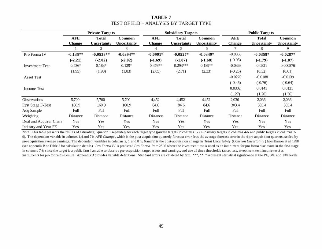
49

TABLE 7

TEST OF H1B – ANALYSIS BY TARGET TYPE

AFE

Change

Total

Uncertainty

Common

Uncertainty

AFE

Change

Total

Uncertainty

Common

Uncertainty

AFE

Change

Total

Uncertainty

Common

Uncertainty

1 2 3 4 5 6 7 8 9

Pro Forma IV -0.135** -0.0538** -0.0394** -0.0991* -0.0527* -0.0349* -0.0358 -0.0358* -0.0287*

(-2.21) (-2.02) (-2.02) (-1.69) (-1.87) (-1.68) (-0.95) (-1.79) (-1.87)

Investment Test 0.436* 0.183* 0.129* 0.476** 0.293*** 0.189** -0.0393 0.0321 0.000876

(1.95) (1.90) (1.83) (2.05) (2.71) (2.33) (-0.25) (0.32) (0.01)

Asset Test -0.0270 -0.0188 -0.0139

(-0.45) (-0.76) (-0.64)

Income Test 0.0302 0.0141 0.0121

(1.27) (1.20) (1.36)

Observations 5,700 5,700 5,700 4,452 4,452 4,452 2,036 2,036 2,036

First Stage F-Test 160.9 160.9 160.9 84.6 84.6 84.6 303.4 303.4 303.4

Acq Sample Full Full Full Full Full Full Full Full Full

Weighting Distance Distance Distance Distance Distance Distance Distance Distance Distance

Deal and Acquirer Chars Yes Yes Yes Yes Yes Yes Yes Yes Yes

Industry and Year FE Yes Yes Yes Yes Yes Yes Yes Yes Yes

Note: This table presents the results of estimating Equation 1 separately for each target type (private targets in columns 1-3, subsidiary targets in columns 4-6, and public targets in columns 7-

9). The dependent variable in columns 1,4 and 7 is AFE Change , which is the post acquisition quarterly forecast error, less the average forecast error in the 4 pre-acquisition quarters, scaled by

pre-acquisition average earnings. The dependent variables in columns 2, 5, and 8 (3, 6 and 9) is the post-acquisition change in Total Uncertainty (Common Uncertainty ) from Barron et al. 1998

(see appendix B or Table 5 for calculation details). Pro Forma IV is predicted Pro Forma from 2SLS where the investment test is used as an instrument for pro forma disclosure in the first stage.

In columns 7-9, since the target is a public firm, I am able to observe pre-acquisition target assets and earnings, and use all three thresholds (asset test, investment test, income test) as

instruments for pro forma disclosure. Appendix B provides variable definitions. Standard errors are clustered by firm. ***, **, * represent statistical significance at the 1%, 5%, and 10% levels.

Private Targets Subsidiary Targets Public Targets

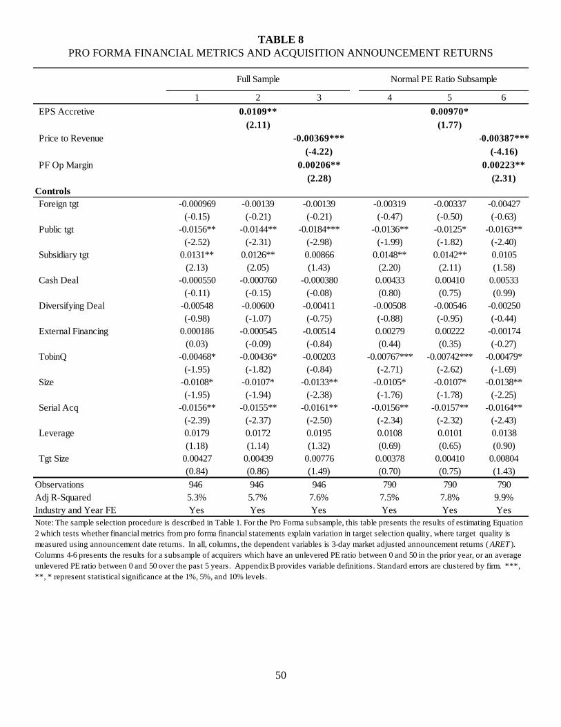
50

TABLE 8

PRO FORMA FINANCIAL METRICS AND ACQUISITION ANNOUNCEMENT RETURNS

1 2 3 4 5 6

EPS Accretive 0.0109** 0.00970*

(2.11) (1.77)

Price to Revenue -0.00369*** -0.00387***

(-4.22) (-4.16)

PF Op Margin 0.00206** 0.00223**

(2.28) (2.31)

Controls

Foreign tgt -0.000969 -0.00139 -0.00139 -0.00319 -0.00337 -0.00427

(-0.15) (-0.21) (-0.21) (-0.47) (-0.50) (-0.63)

Public tgt -0.0156** -0.0144** -0.0184*** -0.0136** -0.0125* -0.0163**

(-2.52) (-2.31) (-2.98) (-1.99) (-1.82) (-2.40)

Subsidiary tgt 0.0131** 0.0126** 0.00866 0.0148** 0.0142** 0.0105

(2.13) (2.05) (1.43) (2.20) (2.11) (1.58)

Cash Deal -0.000550 -0.000760 -0.000380 0.00433 0.00410 0.00533

(-0.11) (-0.15) (-0.08) (0.80) (0.75) (0.99)

Diversifying Deal -0.00548 -0.00600 -0.00411 -0.00508 -0.00546 -0.00250

(-0.98) (-1.07) (-0.75) (-0.88) (-0.95) (-0.44)

External Financing 0.000186 -0.000545 -0.00514 0.00279 0.00222 -0.00174

(0.03) (-0.09) (-0.84) (0.44) (0.35) (-0.27)

TobinQ -0.00468* -0.00436* -0.00203 -0.00767*** -0.00742*** -0.00479*

(-1.95) (-1.82) (-0.84) (-2.71) (-2.62) (-1.69)

Size -0.0108* -0.0107* -0.0133** -0.0105* -0.0107* -0.0138**

(-1.95) (-1.94) (-2.38) (-1.76) (-1.78) (-2.25)

Serial Acq -0.0156** -0.0155** -0.0161** -0.0156** -0.0157** -0.0164**

(-2.39) (-2.37) (-2.50) (-2.34) (-2.32) (-2.43)

Leverage 0.0179 0.0172 0.0195 0.0108 0.0101 0.0138

(1.18) (1.14) (1.32) (0.69) (0.65) (0.90)

Tgt Size 0.00427 0.00439 0.00776 0.00378 0.00410 0.00804

(0.84) (0.86) (1.49) (0.70) (0.75) (1.43)

Observations 946 946 946 790 790 790

Adj R-Squared 5.3% 5.7% 7.6% 7.5% 7.8% 9.9%

Industry and Year FE Yes Yes Yes Yes Yes Yes

Full Sample

Note: The sample selection procedure is described in Table 1. For the Pro Forma subsample, this table presents the results of estimating Equation

2 which tests whether financial metrics from pro forma financial statements explain variation in target selection quality, where target quality is

measured using announcement date returns. In all, columns, the dependent variables is 3-day market adjusted announcement returns ( ARET ).

Columns 4-6 presents the results for a subsample of acquirers which have an unlevered PE ratio between 0 and 50 in the prior year, or an average

unlevered PE ratio between 0 and 50 over the past 5 years. Appendix B provides variable definitions. Standard errors are clustered by firm. ***,

**, * represent statistical significance at the 1%, 5%, and 10% levels.

Normal PE Ratio Subsample

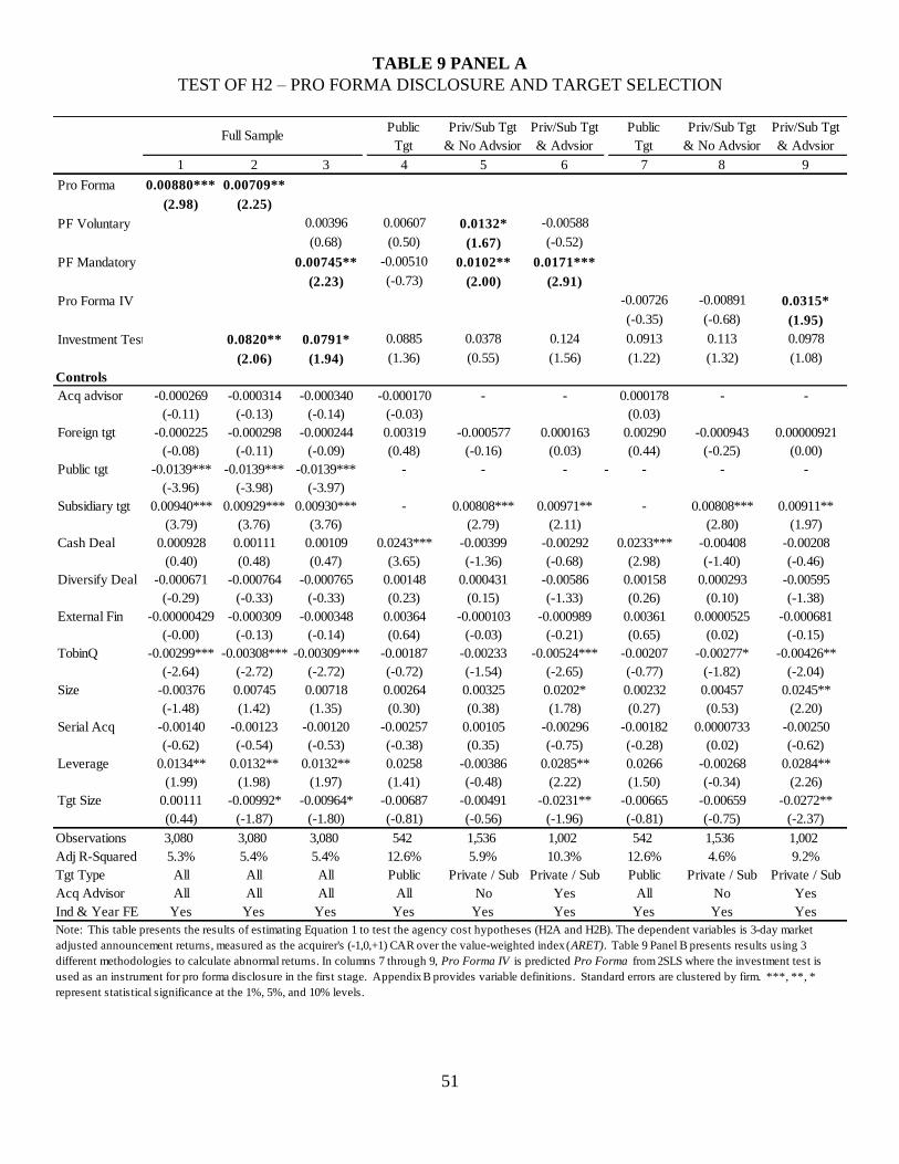
51

TABLE 9 PANEL A

TEST OF H2 – PRO FORMA DISCLOSURE AND TARGET SELECTION

Public

Tgt

Priv/Sub Tgt

& No Advsior

Priv/Sub Tgt

& Advsior

Public

Tgt

Priv/Sub Tgt

& No Advsior

Priv/Sub Tgt

& Advsior

1 2 3 4 5 6 7 8 9

Pro Forma 0.00880*** 0.00709**

(2.98) (2.25)

PF Voluntary 0.00396 0.00607 0.0132* -0.00588

(0.68) (0.50) (1.67) (-0.52)

PF Mandatory 0.00745** -0.00510 0.0102** 0.0171***

(2.23) (-0.73) (2.00) (2.91)

Pro Forma IV -0.00726 -0.00891 0.0315*

(-0.35) (-0.68) (1.95)

Investment Test 0.0820** 0.0791* 0.0885 0.0378 0.124 0.0913 0.113 0.0978

(2.06) (1.94) (1.36) (0.55) (1.56) (1.22) (1.32) (1.08)

Controls

Acq advisor -0.000269 -0.000314 -0.000340 -0.000170 - - 0.000178 - -

(-0.11) (-0.13) (-0.14) (-0.03) (0.03)

Foreign tgt -0.000225 -0.000298 -0.000244 0.00319 -0.000577 0.000163 0.00290 -0.000943 0.00000921

(-0.08) (-0.11) (-0.09) (0.48) (-0.16) (0.03) (0.44) (-0.25) (0.00)

Public tgt -0.0139*** -0.0139*** -0.0139*** - - - - - - -

(-3.96) (-3.98) (-3.97)

Subsidiary tgt 0.00940*** 0.00929*** 0.00930*** - 0.00808*** 0.00971** - 0.00808*** 0.00911**

(3.79) (3.76) (3.76) (2.79) (2.11) (2.80) (1.97)

Cash Deal 0.000928 0.00111 0.00109 0.0243*** -0.00399 -0.00292 0.0233*** -0.00408 -0.00208

(0.40) (0.48) (0.47) (3.65) (-1.36) (-0.68) (2.98) (-1.40) (-0.46)

Diversify Deal -0.000671 -0.000764 -0.000765 0.00148 0.000431 -0.00586 0.00158 0.000293 -0.00595

(-0.29) (-0.33) (-0.33) (0.23) (0.15) (-1.33) (0.26) (0.10) (-1.38)

External Fin -0.00000429 -0.000309 -0.000348 0.00364 -0.000103 -0.000989 0.00361 0.0000525 -0.000681

(-0.00) (-0.13) (-0.14) (0.64) (-0.03) (-0.21) (0.65) (0.02) (-0.15)

TobinQ -0.00299*** -0.00308*** -0.00309*** -0.00187 -0.00233 -0.00524*** -0.00207 -0.00277* -0.00426**

(-2.64) (-2.72) (-2.72) (-0.72) (-1.54) (-2.65) (-0.77) (-1.82) (-2.04)

Size -0.00376 0.00745 0.00718 0.00264 0.00325 0.0202* 0.00232 0.00457 0.0245**

(-1.48) (1.42) (1.35) (0.30) (0.38) (1.78) (0.27) (0.53) (2.20)

Serial Acq -0.00140 -0.00123 -0.00120 -0.00257 0.00105 -0.00296 -0.00182 0.0000733 -0.00250

(-0.62) (-0.54) (-0.53) (-0.38) (0.35) (-0.75) (-0.28) (0.02) (-0.62)

Leverage 0.0134** 0.0132** 0.0132** 0.0258 -0.00386 0.0285** 0.0266 -0.00268 0.0284**

(1.99) (1.98) (1.97) (1.41) (-0.48) (2.22) (1.50) (-0.34) (2.26)

Tgt Size 0.00111 -0.00992* -0.00964* -0.00687 -0.00491 -0.0231** -0.00665 -0.00659 -0.0272**

(0.44) (-1.87) (-1.80) (-0.81) (-0.56) (-1.96) (-0.81) (-0.75) (-2.37)

Observations 3,080 3,080 3,080 542 1,536 1,002 542 1,536 1,002

Adj R-Squared 5.3% 5.4% 5.4% 12.6% 5.9% 10.3% 12.6% 4.6% 9.2%

Tgt Type All All All Public Private / Sub Private / Sub Public Private / Sub Private / Sub

Acq Advisor All All All All No Yes All No Yes

Ind & Year FE Yes Yes Yes Yes Yes Yes Yes Yes Yes

Note: This table presents the results of estimating Equation 1 to test the agency cost hypotheses (H2A and H2B). The dependent variables is 3-day market

adjusted announcement returns, measured as the acquirer's (-1,0,+1) CAR over the value-weighted index (ARET). Table 9 Panel B presents results using 3

different methodologies to calculate abnormal returns. In columns 7 through 9, Pro Forma IV is predicted Pro Forma from 2SLS where the investment test is

used as an instrument for pro forma disclosure in the first stage. Appendix B provides variable definitions. Standard errors are clustered by firm. ***, **, *

represent statistical significance at the 1%, 5%, and 10% levels.

Full Sample

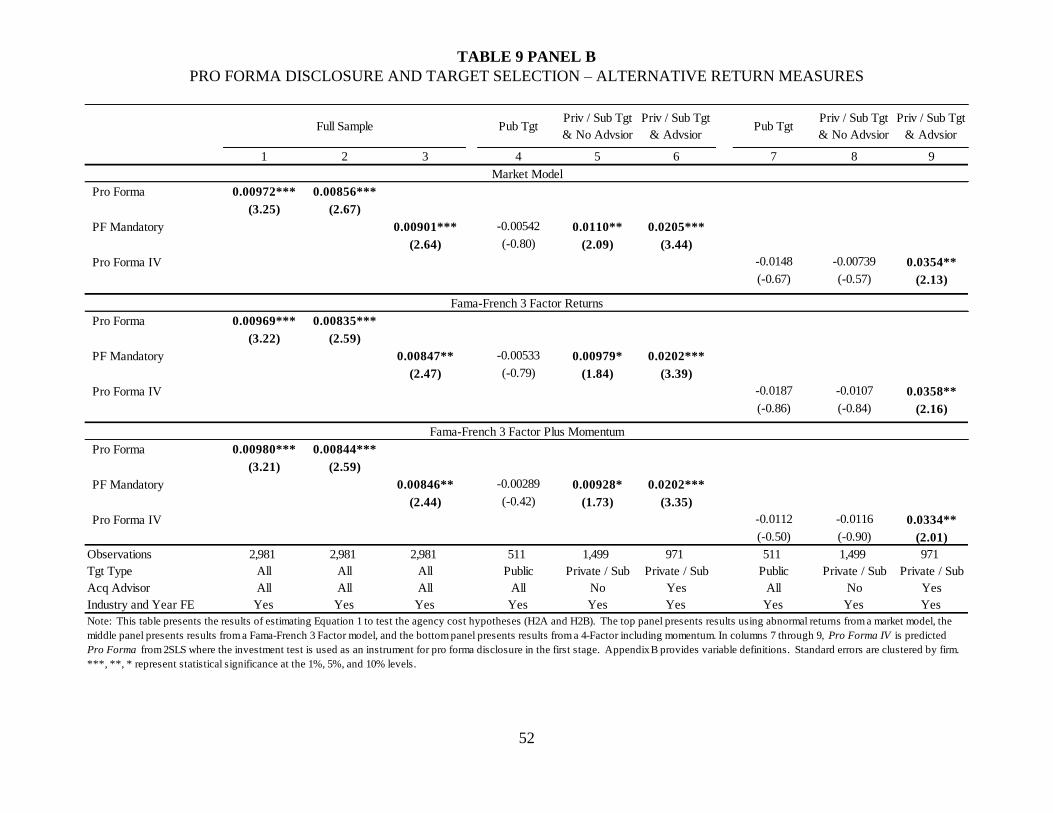
52

TABLE 9 PANEL B

PRO FORMA DISCLOSURE AND TARGET SELECTION – ALTERNATIVE RETURN MEASURES

Pub TgtPriv / Sub Tgt

& No Advsior

Priv / Sub Tgt

& AdvsiorPub Tgt

Priv / Sub Tgt

& No Advsior

Priv / Sub Tgt

& Advsior

1 2 3 4 5 6 7 8 9

Pro Forma 0.00972*** 0.00856***

(3.25) (2.67)

PF Mandatory 0.00901*** -0.00542 0.0110** 0.0205***

(2.64) (-0.80) (2.09) (3.44)

Pro Forma IV -0.0148 -0.00739 0.0354**

(-0.67) (-0.57) (2.13)

Pro Forma 0.00969*** 0.00835***

(3.22) (2.59)

PF Mandatory 0.00847** -0.00533 0.00979* 0.0202***

(2.47) (-0.79) (1.84) (3.39)

Pro Forma IV -0.0187 -0.0107 0.0358**

(-0.86) (-0.84) (2.16)

Pro Forma 0.00980*** 0.00844***

(3.21) (2.59)

PF Mandatory 0.00846** -0.00289 0.00928* 0.0202***

(2.44) (-0.42) (1.73) (3.35)

Pro Forma IV -0.0112 -0.0116 0.0334**

(-0.50) (-0.90) (2.01)

Observations 2,981 2,981 2,981 511 1,499 971 511 1,499 971

Tgt Type All All All Public Private / Sub Private / Sub Public Private / Sub Private / Sub

Acq Advisor All All All All No Yes All No Yes

Industry and Year FE Yes Yes Yes Yes Yes Yes Yes Yes Yes

Note: This table presents the results of estimating Equation 1 to test the agency cost hypotheses (H2A and H2B). The top panel presents results using abnormal returns from a market model, the

middle panel presents results from a Fama-French 3 Factor model, and the bottom panel presents results from a 4-Factor including momentum. In columns 7 through 9, Pro Forma IV is predicted

Pro Forma from 2SLS where the investment test is used as an instrument for pro forma disclosure in the first stage. Appendix B provides variable definitions. Standard errors are clustered by firm.

***, **, * represent statistical significance at the 1%, 5%, and 10% levels.

Market Model

Fama-French 3 Factor Returns

Fama-French 3 Factor Plus Momentum

Full Sample

53

TABLE 10

TEST OF H2 - CONDITIONAL ON ANALYST FOLLOWING

Pub TgtPriv / Sub Tgt

& No Advsior

Priv / Sub Tgt

& AdvsiorPub Tgt

Priv / Sub Tgt

& No Advsior

Priv / Sub Tgt

& Advsior

1 2 3 4 5 6 7 8 9

Pro Forma 0.0151*** 0.0138***

(3.51) (3.07)

PF Mandatory 0.0140*** 0.0197 0.0160*** 0.0170*

(2.93) (1.56) (2.67) (1.71)

Pro Forma IV 0.0375 -0.00221 0.0559*

(1.18) (-0.14) (1.86)

Observations 1,556 1,556 1,556 220 897 439 220 897 439

Adj R-Squared 7.0% 7.1% 7.1% 26.7% 10.2% 12.9% 25.9% 9.0% 8.1%

Pro Forma 0.00256 0.000427

(0.59) (0.09)

PF Mandatory 0.000637 -0.0204** 0.00126 0.0185**

(0.13) (-2.35) (0.13) (2.40)

Pro Forma IV -0.0292 -0.0201 0.0139

(-1.14) (-0.84) (0.75)

Observations 1,524 1,524 1,524 322 639 563 322 639 563

Adj R-Squared 5.7% 6.0% 6.0% 20.5% 4.8% 14.2% 19.7% 2.9% 13.8%

Tgt Type All All All Public Private / Sub Private / Sub Public Private / Sub Private / Sub

Acq Advisor All All All All No Yes All No Yes

Ind & Year FE Yes Yes Yes Yes Yes Yes Yes Yes Yes

Above Median Analyst Following

Note: This table presents the results of testing the agency cost hypotheses (H2A and H2B) separately for below median analyst following (top panel) and above median analyst following (bottom

panel). The dependent variables is 3-day market adjusted announcement returns, measured as the acquirer's (-1,0,+1) CAR over the value-weighted index (ARET). In columns 7 through 9, Pro

Forma IV is predicted Pro Forma from 2SLS where the investment test is used as an instrument for pro forma disclosure in the first stage. Appendix B provides variable definitions. Standard

errors are clustered by firm. ***, **, * represent statistical significance at the 1%, 5%, and 10% levels.

Full Sample

Below Median Analyst Following

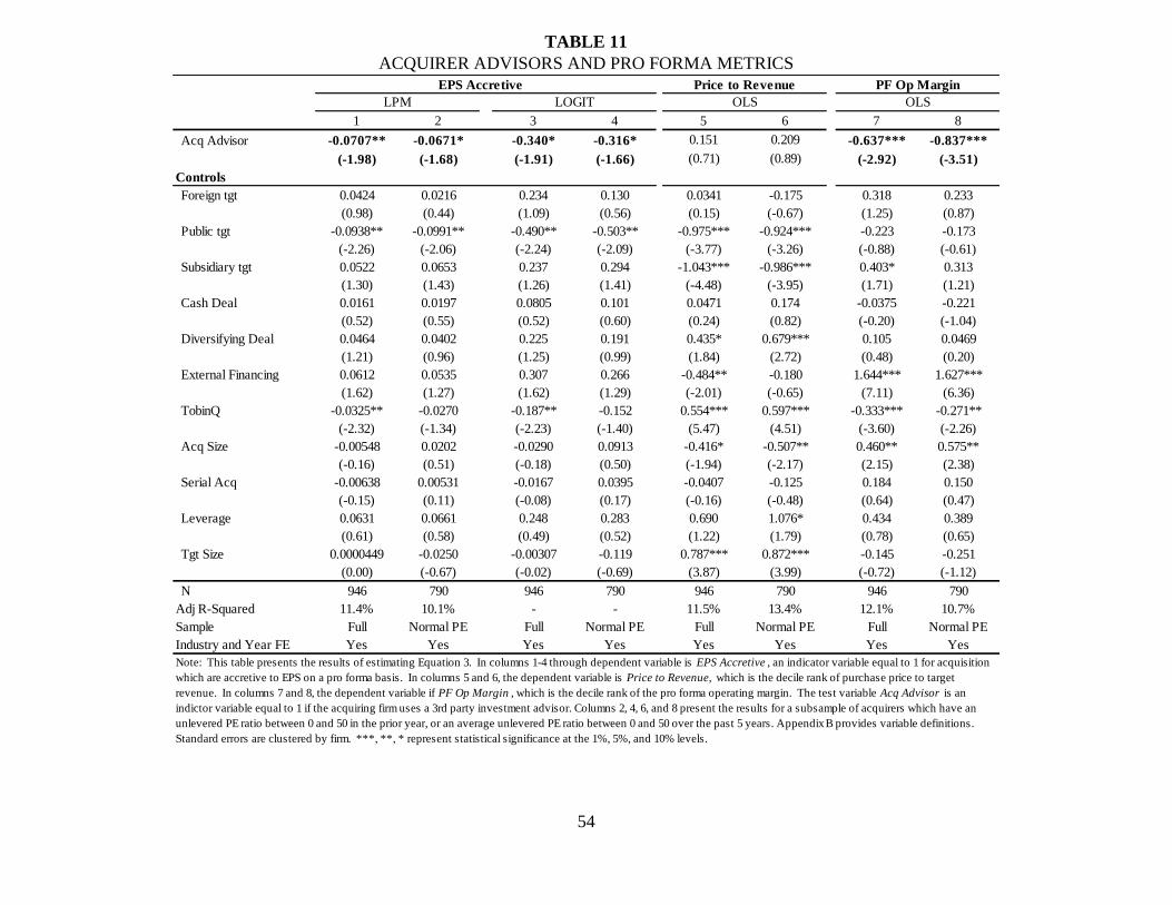
54

TABLE 11

ACQUIRER ADVISORS AND PRO FORMA METRICS

1 2 3 4 5 6 7 8

Acq Advisor -0.0707** -0.0671* -0.340* -0.316* 0.151 0.209 -0.637*** -0.837***

(-1.98) (-1.68) (-1.91) (-1.66) (0.71) (0.89) (-2.92) (-3.51)

Controls

Foreign tgt 0.0424 0.0216 0.234 0.130 0.0341 -0.175 0.318 0.233

(0.98) (0.44) (1.09) (0.56) (0.15) (-0.67) (1.25) (0.87)

Public tgt -0.0938** -0.0991** -0.490** -0.503** -0.975*** -0.924*** -0.223 -0.173

(-2.26) (-2.06) (-2.24) (-2.09) (-3.77) (-3.26) (-0.88) (-0.61)

Subsidiary tgt 0.0522 0.0653 0.237 0.294 -1.043*** -0.986*** 0.403* 0.313

(1.30) (1.43) (1.26) (1.41) (-4.48) (-3.95) (1.71) (1.21)

Cash Deal 0.0161 0.0197 0.0805 0.101 0.0471 0.174 -0.0375 -0.221

(0.52) (0.55) (0.52) (0.60) (0.24) (0.82) (-0.20) (-1.04)

Diversifying Deal 0.0464 0.0402 0.225 0.191 0.435* 0.679*** 0.105 0.0469

(1.21) (0.96) (1.25) (0.99) (1.84) (2.72) (0.48) (0.20)

External Financing 0.0612 0.0535 0.307 0.266 -0.484** -0.180 1.644*** 1.627***

(1.62) (1.27) (1.62) (1.29) (-2.01) (-0.65) (7.11) (6.36)

TobinQ -0.0325** -0.0270 -0.187** -0.152 0.554*** 0.597*** -0.333*** -0.271**

(-2.32) (-1.34) (-2.23) (-1.40) (5.47) (4.51) (-3.60) (-2.26)

Acq Size -0.00548 0.0202 -0.0290 0.0913 -0.416* -0.507** 0.460** 0.575**

(-0.16) (0.51) (-0.18) (0.50) (-1.94) (-2.17) (2.15) (2.38)

Serial Acq -0.00638 0.00531 -0.0167 0.0395 -0.0407 -0.125 0.184 0.150

(-0.15) (0.11) (-0.08) (0.17) (-0.16) (-0.48) (0.64) (0.47)

Leverage 0.0631 0.0661 0.248 0.283 0.690 1.076* 0.434 0.389

(0.61) (0.58) (0.49) (0.52) (1.22) (1.79) (0.78) (0.65)

Tgt Size 0.0000449 -0.0250 -0.00307 -0.119 0.787*** 0.872*** -0.145 -0.251

(0.00) (-0.67) (-0.02) (-0.69) (3.87) (3.99) (-0.72) (-1.12)

N 946 790 946 790 946 790 946 790

Adj R-Squared 11.4% 10.1% - - 11.5% 13.4% 12.1% 10.7%

Sample Full Normal PE Full Normal PE Full Normal PE Full Normal PE

Industry and Year FE Yes Yes Yes Yes Yes Yes Yes Yes

Note: This table presents the results of estimating Equation 3. In columns 1-4 through dependent variable is EPS Accretive , an indicator variable equal to 1 for acquisition

which are accretive to EPS on a pro forma basis. In columns 5 and 6, the dependent variable is Price to Revenue, which is the decile rank of purchase price to target

revenue. In columns 7 and 8, the dependent variable if PF Op Margin , which is the decile rank of the pro forma operating margin. The test variable Acq Advisor is an

indictor variable equal to 1 if the acquiring firm uses a 3rd party investment advisor. Columns 2, 4, 6, and 8 present the results for a subsample of acquirers which have an

unlevered PE ratio between 0 and 50 in the prior year, or an average unlevered PE ratio between 0 and 50 over the past 5 years. Appendix B provides variable definitions.

Standard errors are clustered by firm. ***, **, * represent statistical significance at the 1%, 5%, and 10% levels.

Price to Revenue

OLS OLS

PF Op MarginEPS Accretive

LPM LOGIT

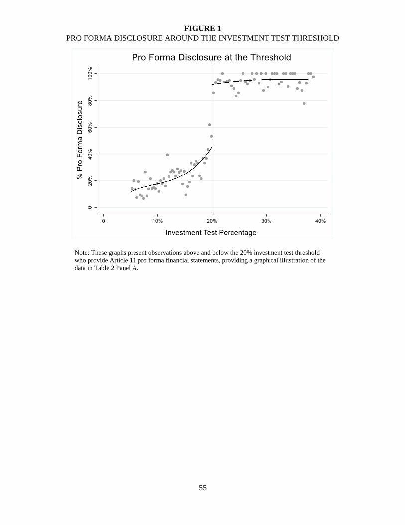
55

FIGURE 1

PRO FORMA DISCLOSURE AROUND THE INVESTMENT TEST THRESHOLD

Note: These graphs present observations above and below the 20% investment test threshold

who provide Article 11 pro forma financial statements, providing a graphical illustration of the

data in Table 2 Panel A.

56

FIGURE 2

THRESHOLD MANIPULATION TEST

Note: The figure above presents the Cattaneo et al. (2017) nonparametric manipulation

test which is designed to test for an abnormal number of observations right above or

below the 20% investment test threshold. The test statistics is -1.26 which equates to a

p-value of 0.21, and I reject manipulation around the threshold. The grey bands

surrounding the fitted lines overlap around the 20% investment test threshold,

providing visual evidence that there is no statistical evidence of manipulation around

the threshold. The table below presents the test statistics for different subsamples.

SampleTest

StatisticP-Value

Evidence of

Manipulation

Full -1.26 0.21 No

Private Tgt -1.46 0.15 No

Public Tgt -0.38 0.71 No

Subsidiary Tgt -0.57 0.57 No

Non-Public Tgt & Outside Advisor -1.23 0.22 No

Non-Public Tgt & No Outside Advisor 0.34 0.73 No

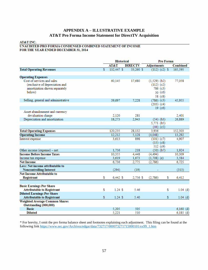
57

APPENDIX A – ILLUSTRATIVE EXAMPLE

AT&T Pro Forma Income Statement for DirectTV Acquisition

* For brevity, I omit the pro forma balance sheet and footnotes explaining each adjustment. This filing can be found at the

following link https://www.sec.gov/Archives/edgar/data/732717/000073271715000101/ex99_1.htm

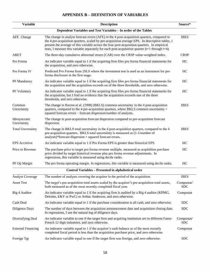
58

APPENDIX B – DEFINITION OF VARIABLES

Variable Description Source*

Dependent Variables and Test Variables – In order of the Tables

AFE Change The change in analyst forecast errors (AFE) in the 4 post-acquisition quarters, compared to

the 4 pre-acquisition quarters, scaled by pre-acquisition average EPS. In descriptive tables, I

present the average of this variable across the four post-acquisition quarters. In empirical

tests, I measure this variable separately for each post-acquisition quarter (t+1 through t+4).

IBES

ARET The three-day cumulative abnormal return (CAR) over the CRSP value-weighted index. CRSP

Pro Forma An indicator variable equal to 1 if the acquiring firm files pro forma financial statements for

the acquisition, and zero otherwise.

HC

Pro Forma IV Predicted Pro Forma from 2SLS where the investment test is used as an instrument for pro

forma disclosure in the first stage.

HC

PF Mandatory An indicator variable equal to 1 if the acquiring firm files pro forma financial statements for

the acquisition and the acquisition exceeds on of the three thresholds, and zero otherwise.

HC

PF Voluntary An indicator variable equal to 1 if the acquiring firm files pro forma financial statements for

the acquisition, but I find no evidence that the acquisition exceeds one of the three

thresholds, and zero otherwise.

HC

Common

Uncertainty

The change in Barron et al. (1998) (BKLS) common uncertainty in the 4 post-acquisition

quarters, compared to the 4 pre-acquisition quarters, where BKLS common uncertainty =

squared forecast errors – forecast dispersion/number of analysts.

IBES

Idiosyncratic

Uncertainty

The change in post-acquisition forecast dispersion compared to pre-acquisition forecast

dispersion.

Total Uncertainty The change in BKLS total uncertainty in the 4 post-acquisition quarters, compared to the 4

pre-acquisition quarters. BKLS total uncertainty is measured as (1-1/number of

analysts)*forecast dispersion + squared forecast errors.

IBES

EPS Accretive An indicator variable equal to 1 if Pro Forma EPS is greater than historical EPS. HC

Price to Revenue The purchase price to target pro forma revenue multiple, measured as acquisition purchase

price divided by target historical revenue plus pro forma revenue adjustments. In

regressions, this variable is measured using decile ranks.

HC

PF Op Margin The pro forma operating margin. In regressions, this variable is measured using decile ranks. HC

Control Variables – Presented in alphabetical order

Analyst Coverage The number of analysts covering the acquirer in the period of the acquisition. IBES

Asset Test The target’s pre-acquisition total assets scaled by the acquirer’s pre-acquisition total assets,

both measured as of the most recently completed fiscal year.

Compustat/

SDC

Big 4 Auditor An indicator variable equal to 1 if the acquiring firm is audited by a Big 4 auditor (KPMG,

Deloitte, E&Y or PwC) or Arthur Anderson, and zero otherwise.

Compustat

Cash Deal An indicator variable equal to 1 if the purchase consideration is all cash, and zero otherwise. SDC

Diligence Days The number of days between the acquisition announcement date and acquisition closing date.

In regressions, I use the natural log of diligence days.

SDC

Diversifying Deal An indicator variable to one if the target firm and acquiring institution are in different Fama-

French 12 digit industries, and zero otherwise.

Compustat/

SDC

External Financing An indicator variable equal to 1 if the acquirer’s cash balance as of the most recently

completed fiscal period is less than the acquisition purchase price, and zero otherwise.

Compustat

Foreign Tgt An indicator variable equal to one if the target firm was foreign, and zero otherwise. SDC

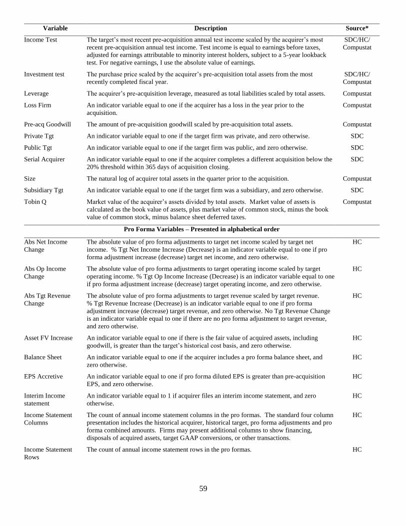
59

Variable Description Source*

Income Test The target’s most recent pre-acquisition annual test income scaled by the acquirer’s most

recent pre-acquisition annual test income. Test income is equal to earnings before taxes,

adjusted for earnings attributable to minority interest holders, subject to a 5-year lookback

test. For negative earnings, I use the absolute value of earnings.

SDC/HC/

Compustat

Investment test The purchase price scaled by the acquirer’s pre-acquisition total assets from the most

recently completed fiscal year.

SDC/HC/

Compustat

Leverage The acquirer’s pre-acquisition leverage, measured as total liabilities scaled by total assets. Compustat

Loss Firm An indicator variable equal to one if the acquirer has a loss in the year prior to the

acquisition.

Compustat

Pre-acq Goodwill The amount of pre-acquisition goodwill scaled by pre-acquisition total assets. Compustat

Private Tgt An indicator variable equal to one if the target firm was private, and zero otherwise. SDC

Public Tgt An indicator variable equal to one if the target firm was public, and zero otherwise. SDC

Serial Acquirer An indicator variable equal to one if the acquirer completes a different acquisition below the

20% threshold within 365 days of acquisition closing.

SDC

Size The natural log of acquirer total assets in the quarter prior to the acquisition. Compustat

Subsidiary Tgt An indicator variable equal to one if the target firm was a subsidiary, and zero otherwise. SDC

Tobin Q Market value of the acquirer’s assets divided by total assets. Market value of assets is

calculated as the book value of assets, plus market value of common stock, minus the book

value of common stock, minus balance sheet deferred taxes.

Compustat

Pro Forma Variables – Presented in alphabetical order

Abs Net Income

Change

The absolute value of pro forma adjustments to target net income scaled by target net

income. % Tgt Net Income Increase (Decrease) is an indicator variable equal to one if pro

forma adjustment increase (decrease) target net income, and zero otherwise.

HC

Abs Op Income

Change

The absolute value of pro forma adjustments to target operating income scaled by target

operating income. % Tgt Op Income Increase (Decrease) is an indicator variable equal to one

if pro forma adjustment increase (decrease) target operating income, and zero otherwise.

HC

Abs Tgt Revenue

Change

The absolute value of pro forma adjustments to target revenue scaled by target revenue.

% Tgt Revenue Increase (Decrease) is an indicator variable equal to one if pro forma

adjustment increase (decrease) target revenue, and zero otherwise. No Tgt Revenue Change

is an indicator variable equal to one if there are no pro forma adjustment to target revenue,

and zero otherwise.

HC

Asset FV Increase An indicator variable equal to one if there is the fair value of acquired assets, including

goodwill, is greater than the target’s historical cost basis, and zero otherwise.

HC

Balance Sheet An indicator variable equal to one if the acquirer includes a pro forma balance sheet, and

zero otherwise.

HC

EPS Accretive An indicator variable equal to one if pro forma diluted EPS is greater than pre-acquisition

EPS, and zero otherwise.

HC

Interim Income

statement

An indicator variable equal to 1 if acquirer files an interim income statement, and zero

otherwise.

HC

Income Statement

Columns

The count of annual income statement columns in the pro formas. The standard four column

presentation includes the historical acquirer, historical target, pro forma adjustments and pro

forma combined amounts. Firms may present additional columns to show financing,

disposals of acquired assets, target GAAP conversions, or other transactions.

HC

Income Statement

Rows

The count of annual income statement rows in the pro formas. HC

60

Variable Description Source*

Leverage Change The change in leverage, measured as pro forma total liabilities scaled by pro forma total

assets minus acquirer historical liabilities scaled by acquirer historical assets.

HC

Neg Op Margin An indicator variable equal to 1 if the pro forma operating margin is negative, and zero

otherwise.

HC

Pro Forma Notes The count of pro forma notes. Each separate letter or number is considered a different pro

forma note.

HC

Tax Rate Decrease An indicator variable equal to one if the pro forma tax rate is smaller than the acquirer’s pre-

acquisition tax rate by 5% or more.

HC

Tax Rate Increase An indicator variable equal to one if the pro forma tax rate is greater than the acquirer’s pre-

acquisition tax rate by 5% or more.

HC

*HC indicates that the data was hand-collected.

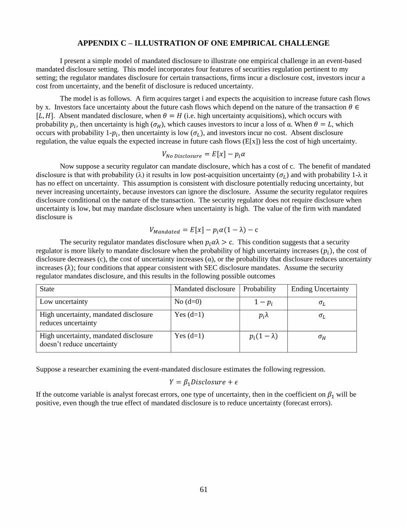
61

APPENDIX C – ILLUSTRATION OF ONE EMPIRICAL CHALLENGE

I present a simple model of mandated disclosure to illustrate one empirical challenge in an event-based

mandated disclosure setting. This model incorporates four features of securities regulation pertinent to my

setting; the regulator mandates disclosure for certain transactions, firms incur a disclosure cost, investors incur a

cost from uncertainty, and the benefit of disclosure is reduced uncertainty.

The model is as follows. A firm acquires target i and expects the acquisition to increase future cash flows

by x. Investors face uncertainty about the future cash flows which depend on the nature of the transaction 𝜃 ∈[𝐿, 𝐻]. Absent mandated disclosure, when 𝜃 = 𝐻 (i.e. high uncertainty acquisitions), which occurs with

probability 𝑝𝑖, then uncertainty is high (𝜎𝐻), which causes investors to incur a loss of α. When 𝜃 = 𝐿, which

occurs with probability 1-𝑝𝑖, then uncertainty is low (𝜎𝐿), and investors incur no cost. Absent disclosure

regulation, the value equals the expected increase in future cash flows (E[x]) less the cost of high uncertainty.

𝑉𝑁𝑜 𝐷𝑖𝑠𝑐𝑙𝑜𝑠𝑢𝑟𝑒 = 𝐸[𝑥] − 𝑝𝑖𝛼

Now suppose a security regulator can mandate disclosure, which has a cost of c. The benefit of mandated

disclosure is that with probability (λ) it results in low post-acquisition uncertainty (𝜎𝐿) and with probability 1-λ it

has no effect on uncertainty. This assumption is consistent with disclosure potentially reducing uncertainty, but

never increasing uncertainty, because investors can ignore the disclosure. Assume the security regulator requires

disclosure conditional on the nature of the transaction. The security regulator does not require disclosure when

uncertainty is low, but may mandate disclosure when uncertainty is high. The value of the firm with mandated

disclosure is

𝑉𝑀𝑎𝑛𝑑𝑎𝑡𝑒𝑑 = 𝐸[𝑥] − 𝑝𝑖𝛼(1 − λ) − c

The security regulator mandates disclosure when 𝑝𝑖𝛼λ > c. This condition suggests that a security

regulator is more likely to mandate disclosure when the probability of high uncertainty increases (𝑝𝑖), the cost of

disclosure decreases (c), the cost of uncertainty increases (α), or the probability that disclosure reduces uncertainty

increases (λ); four conditions that appear consistent with SEC disclosure mandates. Assume the security

regulator mandates disclosure, and this results in the following possible outcomes

State Mandated disclosure Probability Ending Uncertainty

Low uncertainty No (d=0) 1 − 𝑝𝑖 𝜎𝐿

High uncertainty, mandated disclosure

reduces uncertainty

Yes (d=1) 𝑝𝑖λ 𝜎𝐿

High uncertainty, mandated disclosure

doesn’t reduce uncertainty

Yes (d=1) 𝑝𝑖(1 − λ) 𝜎𝐻

Suppose a researcher examining the event-mandated disclosure estimates the following regression.

𝑌 = 𝛽1𝐷𝑖𝑠𝑐𝑙𝑜𝑠𝑢𝑟𝑒 + 𝜖

If the outcome variable is analyst forecast errors, one type of uncertainty, then in the coefficient on 𝛽1 will be

positive, even though the true effect of mandated disclosure is to reduce uncertainty (forecast errors).

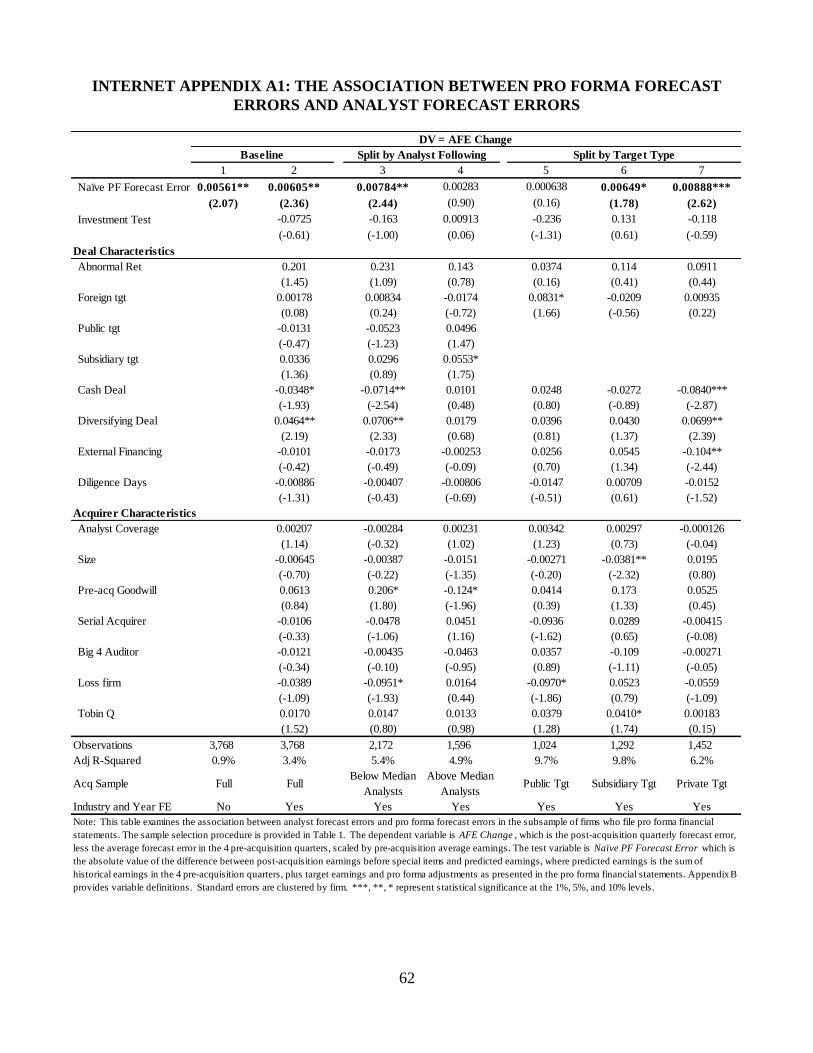
62

INTERNET APPENDIX A1: THE ASSOCIATION BETWEEN PRO FORMA FORECAST

ERRORS AND ANALYST FORECAST ERRORS

1 2 3 4 5 6 7

Naïve PF Forecast Error 0.00561** 0.00605** 0.00784** 0.00283 0.000638 0.00649* 0.00888***

(2.07) (2.36) (2.44) (0.90) (0.16) (1.78) (2.62)

Investment Test -0.0725 -0.163 0.00913 -0.236 0.131 -0.118

(-0.61) (-1.00) (0.06) (-1.31) (0.61) (-0.59)

Deal Characteristics

Abnormal Ret 0.201 0.231 0.143 0.0374 0.114 0.0911

(1.45) (1.09) (0.78) (0.16) (0.41) (0.44)

Foreign tgt 0.00178 0.00834 -0.0174 0.0831* -0.0209 0.00935

(0.08) (0.24) (-0.72) (1.66) (-0.56) (0.22)

Public tgt -0.0131 -0.0523 0.0496

(-0.47) (-1.23) (1.47)

Subsidiary tgt 0.0336 0.0296 0.0553*

(1.36) (0.89) (1.75)

Cash Deal -0.0348* -0.0714** 0.0101 0.0248 -0.0272 -0.0840***

(-1.93) (-2.54) (0.48) (0.80) (-0.89) (-2.87)

Diversifying Deal 0.0464** 0.0706** 0.0179 0.0396 0.0430 0.0699**

(2.19) (2.33) (0.68) (0.81) (1.37) (2.39)

External Financing -0.0101 -0.0173 -0.00253 0.0256 0.0545 -0.104**

(-0.42) (-0.49) (-0.09) (0.70) (1.34) (-2.44)

Diligence Days -0.00886 -0.00407 -0.00806 -0.0147 0.00709 -0.0152

(-1.31) (-0.43) (-0.69) (-0.51) (0.61) (-1.52)

Acquirer Characteristics

Analyst Coverage 0.00207 -0.00284 0.00231 0.00342 0.00297 -0.000126

(1.14) (-0.32) (1.02) (1.23) (0.73) (-0.04)

Size -0.00645 -0.00387 -0.0151 -0.00271 -0.0381** 0.0195

(-0.70) (-0.22) (-1.35) (-0.20) (-2.32) (0.80)

Pre-acq Goodwill 0.0613 0.206* -0.124* 0.0414 0.173 0.0525

(0.84) (1.80) (-1.96) (0.39) (1.33) (0.45)

Serial Acquirer -0.0106 -0.0478 0.0451 -0.0936 0.0289 -0.00415

(-0.33) (-1.06) (1.16) (-1.62) (0.65) (-0.08)

Big 4 Auditor -0.0121 -0.00435 -0.0463 0.0357 -0.109 -0.00271

(-0.34) (-0.10) (-0.95) (0.89) (-1.11) (-0.05)

Loss firm -0.0389 -0.0951* 0.0164 -0.0970* 0.0523 -0.0559

(-1.09) (-1.93) (0.44) (-1.86) (0.79) (-1.09)

Tobin Q 0.0170 0.0147 0.0133 0.0379 0.0410* 0.00183

(1.52) (0.80) (0.98) (1.28) (1.74) (0.15)

Observations 3,768 3,768 2,172 1,596 1,024 1,292 1,452

Adj R-Squared 0.9% 3.4% 5.4% 4.9% 9.7% 9.8% 6.2%

Acq Sample Full FullBelow Median

Analysts

Above Median

AnalystsPublic Tgt Subsidiary Tgt Private Tgt

Industry and Year FE No Yes Yes Yes Yes Yes Yes

Note: This table examines the association between analyst forecast errors and pro forma forecast errors in the subsample of firms who file pro forma financial

statements. The sample selection procedure is provided in Table 1. The dependent variable is AFE Change , which is the post-acquisition quarterly forecast error,

less the average forecast error in the 4 pre-acquisition quarters, scaled by pre-acquisition average earnings. The test variable is Naïve PF Forecast Error which is

the absolute value of the difference between post-acquisition earnings before special items and predicted earnings, where predicted earnings is the sum of

historical earnings in the 4 pre-acquisition quarters, plus target earnings and pro forma adjustments as presented in the pro forma financial statements. Appendix B

provides variable definitions. Standard errors are clustered by firm. ***, **, * represent statistical significance at the 1%, 5%, and 10% levels.

DV = AFE Change

Baseline Split by Analyst Following Split by Target Type

63

INTERNET APPENDIX A2: ACCURACY ENHANCEMENT ROBUSTNESS TESTS

1 2 3 4 5 6 7 8 9

Pro Forma IV -7.057** -7.021** -6.172 -8.544** -8.472** -1.717 -7.662** -7.599** -5.595

(-2.07) (-2.05) (-0.60) (-2.39) (-2.36) (-0.16) (-2.18) (-2.16) (-0.54)

Investment Test 21.06* 21.07* 28.66 29.80** 29.69** -20.82 22.33* 22.15* 17.91

(1.79) (1.77) (0.27) (2.39) (2.36) (-0.19) (1.84) (1.81) (0.17)

Observations 12,320 12,320 2,536 12,320 12,320 2,536 12,320 12,320 2,536

First Stage F-Test 288.2 281.4 26.8 288.2 281.4 26.8 288.2 281.4 26.8

Pro Forma IV -0.140** -0.140** -0.0729 -0.0633** -0.0640** -0.139 -0.0420** -0.0429** -0.109

(-2.31) (-2.30) (-0.39) (-2.45) (-2.45) (-1.41) (-2.23) (-2.25) (-1.50)

Investment Test 0.460** 0.463** -0.276 0.249** 0.254** 1.366 0.150** 0.156** 1.056

(2.08) (2.07) (-0.12) (2.56) (2.57) (1.20) (2.10) (2.13) (1.25)

Observations 6,512 6,512 1,160 6,512 6,512 1,160 6,512 6,512 1,160

First Stage F-Test 157.0 154.4 16.5 157.0 154.4 16.5 157.0 154.4 16.5

Pro Forma IV -0.113*** -0.115*** -0.146 -0.0558*** -0.0566*** -0.0983* -0.0392*** -0.0399*** -0.0736*

(-3.02) (-3.05) (-1.30) (-3.21) (-3.23) (-1.83) (-3.07) (-3.11) (-1.91)

Investment Test 0.406 0.401 4.879 0.239** 0.244** 2.857 0.146* 0.151* 2.735

(1.61) (1.58) (0.78) (2.00) (2.02) (0.94) (1.72) (1.76) (1.25)

Investment Test2 -0.0503 -0.0202 -10.58 -0.0628 -0.0643 -5.616 -0.0226 -0.0252 -5.741

(-0.09) (-0.04) (-0.72) (-0.25) (-0.25) (-0.81) (-0.12) (-0.13) (-1.14)

Observations 12,320 12,320 2,536 12,320 12,320 2,536 12,320 12,320 2,536

First Stage F-Test 356.6 347.9 38.3 356.6 347.9 38.3 356.6 347.9 38.3

Pro Forma IV -0.105*** -0.105*** -0.0749 -0.0498*** -0.0502*** -0.0637 -0.0348*** -0.0353*** -0.0601

(-2.77) (-2.79) (-0.69) (-2.81) (-2.83) (-1.03) (-2.62) (-2.65) (-1.27)

Investment Test 0.362*** 0.365*** 0.0856 0.194*** 0.197*** 0.316 0.123*** 0.126*** 0.352

(2.74) (2.76) (0.08) (3.13) (3.15) (0.53) (2.61) (2.65) (0.75)

Observations 11,912 11,912 2,128 11,912 11,912 2,128 11,912 11,912 2,128

First Stage F-Test 309.2 306.1 38.2 309.2 306.1 38.2 309.2 306.1 38.2

Acq Sample Full Full 15-25% window Full Full 15-25% window Full Full Full

Weighting None Distance Distance None None Distance Distance Distance Distance

Deal and Acquirer Chars Yes Yes Yes Yes Yes Yes Yes Yes Yes

Industry and Year FE Yes Yes Yes Yes Yes Yes Yes Yes Yes

Panel D - Removing Observations Close (within 1%) of the Threshold

Note: This table presents the results four robustness tests related to the accuracy enhancement hypothesis. Panel A shows results measuring outcome variables using percentile ranks. Panel B excludes

acquisitions involving an investment bank which may create a conflict of interest. Panel C includes investment test squared. As suggested by Almond et al. (2011), Panel D removes observations close to

the threshold possibly subject to manipulation. In columns 1-3, the dependent variable is AFE Change , which is the post acquisition quarterly forecast error, less the average forecast error in the 4 pre-

acquisition quarters, scaled by pre-acquisition average earnings. In columns 4-6 (7-9) the dependent variables is the post-acquisition change in Total Uncertainty (Common Uncertainty ) from Barron et

al. 1998 (see appendix B or Table 5 for calculation details). Pro Forma IV is predicted Pro Forma from 2SLS where the investment test is used as an instrument for pro forma disclosure in the first stage.

Standard errors are clustered by firm. ***, **, * represent statistical significance at the 1%, 5%, and 10% levels.

Panel B - Non-Advisor Acquisitions Subsample Robustness Test

DV = AFE Change DV = Total Uncertainty DV = Common Uncertainty

Panel A - Measuring the Dependent Variable in Percentile Ranks

Panel C - Including Higher Order Polynomials of the Investment Test