THE ANALYSIS OF HOUSEHOLD SURVEYS A Microeconometric Approach to Development Policy Angus Deaton Published for the World Bank The Johns Hopkins University Press Baltimore and London

Welcome message from author
This document is posted to help you gain knowledge. Please leave a comment to let me know what you think about it! Share it to your friends and learn new things together.
Transcript

THE ANALYSIS OF
HOUSEHOLD
SURVEYS
A Microeconometric Approach
to Development Policy
Angus Deaton
Published for the World BankThe Johns Hopkins University Press
Baltimore and London

2 Econometric issuesfor survey data
This chapter, like the previous one, lays groundwork for the analysis to follow.The approach is that of a standard econometric text, emphasizing regression anal-ysis and regression "diseases" but with a specific focus on the use of survey data.The techniques that I discuss are familiar, but I focus on the methods and variantsthat recognize that the data come from surveys, not experimental data nor timeseries of macroeconomic aggregates, that they are collected according to specificdesigns, and that they are typically subject to measurement error. The topics arethe familiar ones; dependency and heterogeneity in regression residuals, and pos-sible dependence between regressors and residuals. But the reasons for theseproblems and the contexts in which they arise are often specific to survey data.For example, the weighting and clustering issues with which I begin do not occurexcept in survey data, although the methodology has straightforward parallelselsewhere in econometrics.
What might be referred to as the "econometric" approach is not the only wayof thinking about regressions. In Chapter 3 and at several other points in thisbook, I shall emphasize a more statistical and descriptive methodology. Since thedistinction is an important one in general, and since it separates the material inthis chapter from that in the next, I start with an explanation. The statistical ap-proach comes first, followed by the econometric approach. The latter is developedin this chapter, the former in Chapter 3 in the context of substantive applications.
From the statistical perspective, a regression or "regression function" is de-fined as an expectation of one variable, conventionally written y, conditional onanother variable, or vector of variables, conventionally written x. I write this inthe standard form
(2.1) m(x) = E(ylx) = fydFc(ylx)
where FC is the distribution function of y conditional on x. This definition of a re-gression is descriptive and carries no behavioral connotation. Given a set of vari-ables (y,x) that are jointly distributed, we can pick out one that is of interest, inthis case y, compute its distribution conditional on the others, and calculate theassociated regression function. From a household survey, we might examine the
63

64 THE ANALYSIS OF HOUSEHOLD SURVEYS
regression of per capita expenditure (y) on household size (x), which would beequivalent to a tabulation of mean per capita expenditure for each household size.But we might just as well examine the reverse regression, of household size onper capita expenditure, which would tell us the average household size at differentlevels of resources per capita. In such a context, the estimation of a regression isprecisely analogous to the estimation of a mean, albeit with the complication thatthe mean is conditioned on the prespecified values of the x-variables. When wethink of the regression this way, it is natural to consider not only the conditionalmean, but other conditional measures, such as the median or other percentiles,and these different kinds of regression are also useful, as we shall see below.Thinking of a regression as a set of means also makes it clear how to incorporateinto regressions the survey design issues that I discussed at the end of Chapter 1.
When the conditioning variables in the regression are continuous, or whenthere is a large number of discrete variables, the calculations are simplified if weare prepared to make assumptions about the functional form of m(x). The mostobvious and most widely used assumption is that the regression function is linearin x,
(2.2) m(x) = fYx
where P is a scalar or vector as x is a scalar or vector, and where, by defining oneof the elements of x to be a constant, we can allow for an intercept term. In thiscase, the ,B-parameters can be estimated by ordinary least squares (OLS), and theestimates used to estimate the regression function according to (2.2).
The econometric approach to regression is different, in rhetoric if not in real-ity. The starting point is usually the linear regression model
(2.3) y = f'x + u
where u is a "residual," "disturbance," or "error" term representing omitted deter-minants of y, including measurement error, and satisfying
(2.4) E(ulx) = 0.
The combination of (2.3) and (2.4) implies that 'x is the expectation of y condi-tional on x, so that (2.3) and (2.4) imply the combination of (2.1) and (2.2). Simi-larly, because a variable can always be written as its expectation plus a residualwith zero expectation, the combination of (2.1) and (2.2) imply the combinationof (2.3) and (2.4). As a result, the statistical and econometric approaches are for-mally identical. The difference lies in the rhetoric, and particularly in the contrastbetween "model" and "description." The linear regression as written in (2.3) and(2.4) is often thought of as a model of determination, of how the "independent"variables x determine the "dependent" variable y. By contrast, the regressionfunction (2.1) is more akin to a cross-tabulation, devoid of causal significance, adescriptive device that is (at best) a preliminary to more "serious," or model-based, analysis.
ECONOMETRIC ISSUES FOR SURVEY DATA 65
A good example of the difference comes from the analysis of poverty, whereregression methods have been applied for a very long time (see Yule 1899). Sup-pose that the variable y, is 1 if household i is in poverty and is 0 if not. Supposethat the conditioning variables x are a set of dummy variables representing re-gions of a country. The coefficients of a linear regression of y on x are then a"6poverty profile,'' the fractions of households in poverty in each of the regions.These results could also have been represented by a table of means by region, ora regression function. A poverty profile can incorporate more than regional infor-mation, and might include local variables, such as whether or not the communityhas a sealed road or an irrigation system, or household variables, such as theeducation of the household head. Such regressions answer questions about differ-ences in poverty rates between irrigated and unirrigated villages, or the extent towhich poverty is predicted by low education. They are also useful for targetingantipoverty policies, as when transfers are conditioned on geography or on land-holding (see, for example, Grosh 1994 or Lipton and Ravallion 1995.) Of course,such descriptions are not informative about the determinants of poverty. House-holds in communities with sealed roads may be well-off because of the tradebrought by the road, or the road may be there because the inhabitants have theeconomic wherewithal to pay for it, or the political power to have someone elsedo so. Correlation is not causation, and while poverty regressions are excellenttools for constructing poverty profiles, they do not measure up to the more rigor-ous demands of project evaluation.
Much of the theory and practice of econometrics consists of the developmentand use of tools that permit causal inference in nonexperimental data. Althoughthe regression of individual poverty on roads cannot tell us whether or by howmuch the construction of roads will reduce poverty, there exist techniques thathold out the promise of being able to do so, if not from an OLS regression, at leastfrom an appropriate modification. Econometric theorists have constructed a cata-log of regression "diseases," the presence of any of which can prevent or distortcorrect inference of causality. For each disease or combination of diseases, thereexist techniques that, at least under ideal conditions, cart repair the situation.Econometrics texts are largely concerned with these techniques, and their applica-tion to survey data is the main topic of this chapter.
Nevertheless, it pays to be skeptical and, in recent years, many economists andstatisticians have become increasingly dissatisfied with technical fixes, and inparticular, with the strong assumptions that are required for them to work. In atleast some cases, the conditions under which a procedure will deliver the rightanswer are almost as implausible, and as difficult to validate, as those required forthe original regression. Readers are referred to the fine skeptical review by Freed-man (1991), who concludes "that statistical technique can seldom be an adequatesubstitute for good design, relevant data, and testing predictions against reality ina variety of settings." One of my aims in this chapter is to clarify the often ratherlimited conditions under which the various econometric techniques work, and toindicate some more realistic alternatives, even if they promise less. A good start-ing point for all econometric work is the (obvious) realization that it is not always

66 THE ANALYSIS OF HOUSEHOLD SURVEYS
possible to make the desired inferences with the data to hand. Nevertheless, evenif we must sometimes give up on causal inference, much can be learned fromcareful inspection and description of data, and in the next chapter, I shall discusstechniques that are useful and informative for this more modest endeavor.
This chapter is organized as follows. There are nine sections, the last of whichis a guide to further reading. The first two pick up from the material at the end ofChapter I and look at the role of survey weights (Section 2.1) and clustering (Sec-tion 2.2) in regression analysis. Section 2.3 deals with the fact that regressionfunctions estimated from survey data are rarely homoskedastic, and I presentbriefly the standard methods for dealing with the fact. Quantile regressions areuseful for exploring heteroskedasticity (as well as for many other purposes), andthis section contains a brief presentation. Although the consequences of hetero-skedasticity are readily dealt with in the context of regression analysis, the sameis not true when we attempt to use the various econometric methods designed todeal with limited dependent variables. Section 2.4 recognizes that survey data arevery different from the controlled experimental data that would ideally be re-quired to answer many of the questions in which we are interested. I review thevarious econometric problems associated with nonexperimental data, includingthe effects of omitted variables, measurement error, simultaneity, and selectivity.Sections 2.5 and 2.6 review the uses of panel data and of instrumental variables(IV), respectively, as a means to recover structure from nonexperimental data.Section 2.7 shows how a time series of cross-sectional surveys can be used to ex-plore changes over time, not only for national aggregates, but also for socioeco-nomic groups, especially age cohorts of people. Indeed, such data can be used inways that are similar to panel data, but without some of the disadvantages-parti-cularly attrition and measurement error. I present some examples, and discusssome of the associated econometric issues. Finally, section 2.8 discusses twotopics in statistical inference that will arise in the empirical work in later chapters.
2.1 Survey design and regressions
As we have already seen in Section 1.1, there are both statistical and practical rea-sons for household surveys to use complex designs in which different householdshave different probabilities of being selected into the sample. We have also seenthat such designs have to be taken into account when calculating means and otherstatistics, usually by weighting, and that the calculation of standard errors for theestimates should depend on the sample design. We also saw that, standard errorscan be seriously misleading if the sample design is not taken into account in theircalculation, particularly in the case of clustered samples. In this section, I take upthe same questions in the context of regressions. I start with the use of weights,and with the old and still controversial issue of whether or not the survey weightsshould be used in regression. As we shall see, the answer depends on what onethinks about and expects from a regression, and on whether one takes an econo-metric or statistical view. I then consider the effects of clustering, and show thatthere is no ambiguity about what to do in this case; standard errors should be cor-
ECONOMETRIC ISSUES FOR SURVEY DATA 67
rected for the design. I conclude the section with a brief overview of regressionstandard errors and sample design, going beyond clustering to the effects of strati-fication and probability weighting.
Weighting in regressions
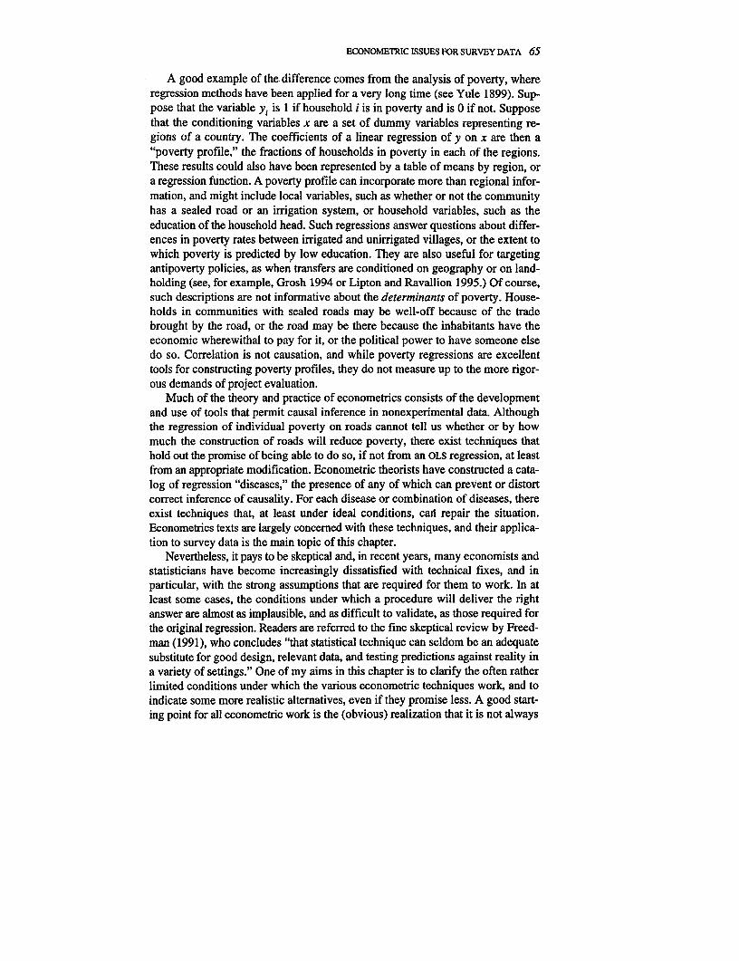
Consider a sample in which households belong to one of S "sectors," and wherethe probability of selection into the sample varies from sector to sector. In thesimplest possible case, there are two sectors, for example, rural and urban, thesample consists of rural and urban households, and the probability of selection ishigher in the urban sector. The sectors will often be sample strata, but my concernhere is with variation in weights across sectors-however defined-and not di-rectly with stratification. If the means are different by sector, we know that theunweighted sample mean is a biased and inconsistent estimator of the populationmean, and that a consistent estimator can be constructed by weighting the indivi-dual observations by inflation factors, or equivalently, by computing the meansfor each sector, and weighting them by the fractions of the population in each.The question is whether and how this procedure extends from the estimation ofmeans to the estimation of regressions.
Suppose that there are Ns population households and n, sample households insector s. With simple random sampling within sectors, the inflation factor for ahousehold i in s is w,, = N/In,, so that the weighted mean (1.25) is
s ns s
Z 1 SWj8xjs E sX NSX( -= i=_ X= = L. -X = X.
(2.5) W S S N
s=li=l s=l
Hence, provided that the sample means for each sector are unbiased for the cor-responding population means, so is the weighted mean for the overall populationmean. Equation (2.5) also shows that it makes no difference whether we take aweighted mean of individual observations with inflation factors as weights, orwhether we compute the sector means first, and then weight by population shares.
Let us now move to the case where the parameters of interest are no longerpopulation totals or means, but the parameters of a linear regression model. With-in each sector s = 1, . . S,
(2.6) YS = XjP3 + X5
and, in general, the parameter vectors P, differ across sectors. In such a case, wemight decide, by analogy with the estimation of means, that the parameter ofinterest is the population-weighted average
(2.7) B = N-1 EN,.s=l

68 THE ANALYSIS OF HOUSEHOLD SURVEYS
Consider the only slightly artificial example where the regressions are Engelcurves for a subsidized food, such as rice, and we are interested in the effects of ageneral increase in income on the aggregate demand for rice, and thus on the totalcost of the subsidy. If the marginal propensity to spend on rice varies from onesectors to another, then (2.7) gives the population average, which is the quantitythat we need to know.
Again by analogy with the estimation of means, we might proceed by estimat-ing a separate regression for each sector, and weighting them together using thepopulation weights. Hence,
s N(2.8) = . N 0' = (X,'X,)Q Xy,
.V= N
Such regressions are routinely calculated when the sectors are broad, such as inthe urban versus rural example, and where there are good prior reasons for sup-posing that the parameters differ across sectors. Such a procedure is perhaps lessattractive when there is little interest in the individual sectoral parameter esti-mates, or when there are many sectors with few households in each, so that theparameters for each are estimated imprecisely. But such cases arise in practice;some sample designs have hundreds of strata, chosen for statistical or adminis-trative rather than substantive reasons, and we may not be sure that the parametersare the same in each stratum. If so, the estimator (2.8) is worth consideration, andshould not be rejected simply because there are few observations per stratum. Ifthe strata are independent, the variance of 3 is
(2.9) V(j3) = E( V() =E (X,
where oa2 is the residual variance in stratum s. Because the population fractions in(2.9) are squared, 0 will be more precisely estimated than are the individual 0.
Instead of estimating parameters sector by sector, it is more common to esti-mate a regression from all the observations at once, either using the inflationfactors to calculate a weighted least squares estimate, or ignoring them, and esti-mating by unweighted OLS. The latter can be written
(2.10) =(E X
In general, the OLS estimator will not yield any parameters of interest. Supposethat, as the sample size grows, the moment matrices in each stratum tend to finitelimits, so that we can write
(2.11) plim n,')X,'XS = M.; plim n 'X(y' = cS = MTPSn,-. n,--
where M, and c, are nonrandom and the former is positive definite. (Note that, asin Chapter 1, I am assuming sampling with replacement, so that it is possible tosample an infinite number from a finite population.) By (2.11), the probabilitylimit of the OLS estimator (2.10) is

ECONOMETRIC ISSUES FOR SURVEY DATA 69
(2.12) plim, = ( nS/n) Ms) l (ns,n)Css=I s=1
where I have assumed that, as the sample size grows, the proportions in eachsector are held fixed. If all the Ps are the same, so that c5 = Ms P for all s, then theOLS estimator will be consistent for the common P. However, even if the structureof the explanatory variables is the same in each of the sectors, so that M. = M forall s and cs = MP3s, equation (2.12) gives the sample-weighted average of the P,which is inconsistent unless the sample is a simple random sample with equalprobabilities of selection in all sectors.
The inconsistency of the OLS estimator for the population parameters mirrorsthe inconsistency of the unweighted mean for the population mean. Consider thenthe regression counterpart of the weighted mean, in which each household'scontribution to the moment matrices is inflated using the weights,
(2.13) 3w E S iSis) ( E wisxisYis)s=l i=l s=l i=l
where x1, is the vector of explanatory variables for household i in sector s, and Y',is the corresponding value of the dependent variable. In this case, the weights are N.1n,and vary only across sectors, so that the estimator can also be written as
(2.14) ( = ( = (X'WXYSX'Wy
where X and y have their usual regression connotations-the X. and y5 matricesfrom each sector stacked vertically-and W is an n x n matrix with the weightsNslns on the diagonal and zeros elsewhere. This is the weighted regression that iscalculated by regression packages, including STATA.
If we calculate the probability limits as before, we get instead of (2.12)
(2.15) plimn = ( .NMS -1 SIINMsPS
so that, where we previously had sample shares as weights, we now have popu-lation shares. The weighted estimator thus has the (perhaps limited) advantageover the OLS estimator of being independent of sample design; the right-hand sideof (2.15) contains only population magnitudes. Like the OLS estimator it is consis-tent if all the , are identical, and unlike it, will also be consistent if the Ms mat-rices are identical across sectors. We have already seen one such case; when thereis only a constant in the regression, Ms = 1 for all s, and we are estimating thepopulation mean, where weighting gives the right answer. But it is hard to thinkof other realistic examples in which the M, are common and the c5 differ. In gen-eral, the weighted estimator will not be consistent for the weighted sum of theparameter vectors because
70 THE ANALYSIS OF HOUSEHOLD SURVEYS
- S A I S S S
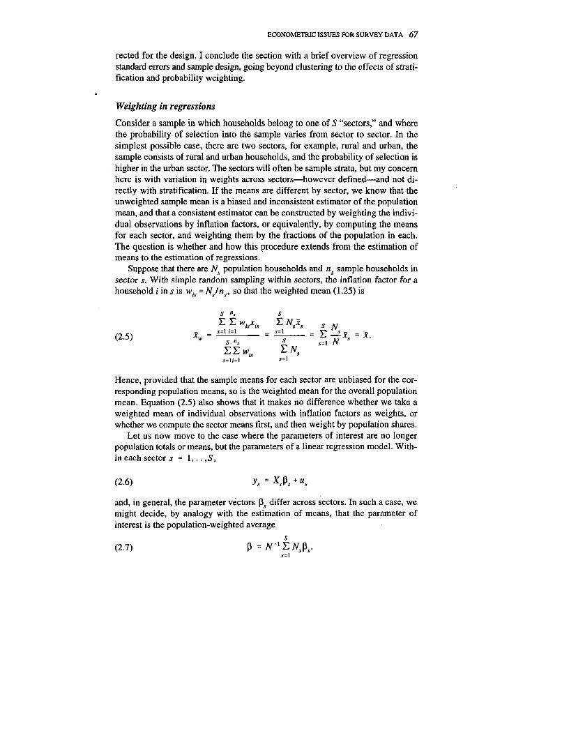
(2.16) E (N,1N)Ms (NsIN)c, o E(Ns1N)Is1C5= ((Ns/N)ps = P.2 s=. s= s=1 s=l
In this case, which is probably the typical one, there is no straightforward analogybetween the estimation of means and the estimation of regression parameters. Theweighted estimator, like the OLS estimator, is inconsistent.
As emphasized by Dumouchel and Duncan (1983), the weighted OLS estimatorwill be consistent for the parameters that would have been estimated using censusdata; as usual, the weighting makes the sample look like the population and re-moves the dependence of the estimates on the sample design, at least when sam-ples are large enough. However, the difference in parameter values across strata isa feature of the population, not of the sample design, so that running a regressionon census data is no less problematic than running it on sample data. In neithercase can we expect to recover parameters of interest. The issue is not sampledesign, but population heterogeneity. Of course, if the population is homoge-neous, so that the regression coefficients are identical in each stratum, bothweighted and unweighted estimators will be consistent. In such a case, and in theabsence of other problems, the unweighted OLS estimator is to be preferred since,by the Gauss-Markov theorem, least squares is more efficient than the weightedestimator. This is the classic econometric argument against the weighted estima-tor: when the sectors are homogeneous, OLS is more efficient, and when they arenot, both estimators are inconsistent. In neither case is there an argument forweighting.
Even so, it is possible to defend the weighted estimator. I present one argu-ment that is consistent with the modeling point of view, and one that is not. Sup-pose that there are many sectors, that we suspect heterogeneity, but the heteroge-neity is not systematically linked to the other variables. Consider again the proba-bility limit of the weighted estimator, (2.15), substitute cc=MAP, and writePs = P + (P - P) to reach
s ~~~~I s(2.17) plimno = P+ ( (N/N)M) E (Ns/N)M5 (Ps-P).
s=l ~~~~s=lThe weighted estimate will therefore be consistent for P if
s(2.18) I (N5 /N)Ms (P., -P) = 0.
This will be the case if the variation in the parameters across sectors is randomand is unrelated to the moment matrices Ms in each, and if the number of sectorsis large enough for the weighted mean to be zero. The same kind of argument ismuch harder to make for the unweighted (oLs) estimator. The orthogonality con-dition (2.18) is a condition on the population, while the corresponding conditionfor the OLS estimator would have to hold for the sample, so that the estimatorwould (at best) be consistent for only some sampling schemes. Even then, itsprobability limit would not be P but the sample-weighted mean of the sector-specific Ps, a quantity that is unlikely to be of interest.

ECONOMETRIC ISSUES FOR SURVEY DATA 71
Perhaps the strongest argument for weighted regression comes from those whoregard regression as descriptive, not structural. The case has been put forcefullyby Kish and Frankel (1974), who argue that regression should be thought of as adevice for summarizing characteristics of the population, heterogeneity and all, sothat samples ought to be weighted and regressions calculated according to (2.13)or (2.14). A weighted regression provides a consistent estimate of the populationregression function-provided of course that the assumption about functionalform (in this case that it is linear) is correct. The argument is effectively that theregression function itself is the object of interest. I shall argue in the next chapterthat this is frequently the case, both for the light that the regression functionsometimes sheds on policy, and when not, as a preliminary description of thedata. Of course, if we are trying to estimate behavioral models, and if those mod-els are different in different parts of the population, the classic econometric argu-ment is correct, and weighting is at best useless.
Recommendationsforpractice
How then should we proceed? Should the weights be ignored, or should we usethem in the regressions? What about standard errors? If regressions are primarilydescriptive, exploring association by looking at the mean of one variable condi-tional on others, the answer is straightforward: use the weights and correct thestandard errors for the design. For modelers who are concerned about heterogene-ity and its interaction with sample design, matters are somewhat more compli-cated.
For descriptive purposes, the only issue that I have not dealt with is the com-putation of standard errors. In principle, the techniques of Section 1.4 can be usedto give explicit formulas that take into account the effect of survey design on thevariance-covariance matrices of parameter estimates. At the time of writing, suchformulas are being incorporated into STATA. Alternatively, the bootstrap providesa computationally intensive but essentially mechanical way of calculating stand-ard errors, or at least for checking that the standard errors given by the conven-tional formulas are not misleading. As in Section 1.4, the bootstrap should be pro-grammed so as to reflect the sample design: different strata should be bootstrap-ped separately and, for two-stage samples, bootstrap draws should be made ofclusters or primary sampling units (PSUs), not of the households within them.Because hypothetical replications of the survey throw up new households at eachreplication, with new values of x's as well as y's, the bootstrap should do thesame. In this context, it makes no sense to condition on the original x's, holdingthem fixed in repeated samples. Instead, each bootstrap sample will contain aresampling of households, with their associated x's, y's, and weights w's, andthese are used to compute each bootstrap regression.
In practice, the design feature that usually has the largest effect on standarderrors is clustering, and the most serious problem with the conventional formulasis that they overstate precision by ignoring the dependence of observations withinthe same Psu. We have already seen this phenomenon for estimation of the mean

72 THE ANALYSIS OF HOUSEHOLD SURVEYS
in Section 1.4, and it is sufficiently important that I shall return to it in Section 2.2below. It is as much an issue for structural estimation as it is for the use of regres-sions as descriptive tools.
The regression modeler has a number of different strategies for dealing withheterogeneity and design. At one extreme is what might be called the standardapproach. Behavior is assumed to be homogeneous across (statistical or substan-tive) subunits, the data are pooled, and the weights ignored. The other extreme isto break up the sample into cells whenever behavior is thought likely to differ orwhere the sampling weights differ across groups. Separate regressions are thenestimated for each cell and the results combined using population weights accord-ing to (2.8). When the distinctions between groups are of substantive interest-aswill often be the case, since regions, sectors, or ethnic characteristics are oftenused for stratification-it makes sense to test for differences between them usingcovariance analysis, as described, for example, by Johnston (1972, pp. 192-207).
When adopting the standard approach, it is also wise to adopt Dumouchel andDuncan's suggestion of calculating both weighted and unweighted estimators andcomparing them. Under the null that the regressions are homogeneous acrossstrata, both estimators are unbiased, so that the difference between them has anexpectation of zero. By contrast, when heterogeneity and design effects are im-portant, the two expectations will differ. The difference between the weightedestimator (2.13) and the OLS estimator can be written as
tOOS = (X'WX)'1X'Wy -(X'X)IX'y(2.19) = (X'WX)Y'X'W(I-X(X'X) 'X ')y
= (X 'WX) -IX /WMXy
where Mx is the matrix I-X(X'X)-yX'. By (2.19) the difference between the twoestimators is the vector of parameter estimates from a weighted regression of theunweighted OLS residuals on the x's. Its variance-covariance matrix can readily becalculated in order to form a test statistic, but the easiest way to test whether(2.19) is zero is to run the "auxiliary" regression
(2.20) y = Xb + WXg+v
and to use an F-statistic to test g = 0 (see also Davidson and MacKinnon 1993.pp. 237-42, who discuss Hausman (1978) tests, of which this is a special case).
In the case of many sectors, when we rely on the interpretation that the inter-sectoral heterogeneity is random variation in the parameters as in (2.17) above,note that the residuals of the regressions, whether weighted or unweighted, will beboth heteroskedastic and dependent. Rewrite the regressions (2.6) as
(2.21) Y, = XV (p-i + U., = V + E.,
where , is defined in (2.7) and where the compound residual is is defined by thesecond equality. If the intrasectoral variance-covariance matrix of the P, is Q,
ECONOMETRIC ISSUES FOR SURVEY DATA 73
the variances and covariances of the new residuals are zero between residuals indifferent sectors, while within each sector we have
(2.22) E(t, C$) = X (,X' + a21
where I is the n,xn. identity matrix. Hence, if the different sectors in (2.21) arecombine'd, or "stacked," into a single regression, the variance-covariance matrixof the residuals will have a block diagonal structure, displaying both heteroske-dasticity and intercorrelation. In such circumstances, neither the weighted norunweighted regressions will be efficient, and perhaps more seriously, the standardformulas for the estimated standard errors will be incorrect. In the next two sec-tions, we shall see how to detect and deal with these problems in a slightly differ-ent but mathematically identical context.
2.2 The econometrics of clustered samples
In Chapter 1, we saw that most household surveys in developing countries use atwo-stage design, in which clusters or Psus are drawn first, followed by a selec-tion of households from within each PsU. In Section 1.4, I explored the conse-quences of clustered designs for the estimation of means and their standard errors.Here I discuss the use of clusters in empirical work more broadly. When the sur-vey data are gathered from rural areas in developing countries, the clustering isoften of substantive interest in its own right. I begin with some of these positiveaspects of clustered sampling, and then discuss its effects on inference in regres-sion analysis.
The economics of clusters in developing countries
In surveys of rural areas in developing countries, clusters are often villages, sothat households in a single cluster live near one another, and are interviewed atmuch the same time during the period that the survey team is in the village. Inmany countries, these arrangements will produce household data where obser-vations from the same cluster are much more like one another than are observa-tions from different clusters. At the simplest, there may be neighborhood effects,so that local eccentricities are copied by those who live near one another and be-come more or less uniform within a village. Sample villages are often widelyseparated geographically, their inhabitants may belong to different ethnic andreligious groups, they may have distinct occupational structures as well as differ-ent crops and cropping patterns. Where agriculture is important-as it is in mostpoor countries-there will usually be more homogeneity within villages than bet-ween them. This applies not only to the types of crops and livestock, but also tothe effects of weather, pests, and natural hazards. If the rains fail for a particularvillage, everyone engaged in rainfed agriculture will suffer, as will those in occu-pations that depend on rainfed agriculture. If the harvest is good, prices will below for everyone in the village, and although the effects will spread out to other

74 THE ANALYSIS OF HOUSEHOLD SURVEYS
villages through the market, poor transport networks and high transport costs maylimit the spread of low prices to other survey villages. Indeed, there is often onlyone market in each village, so that everyone in the village will be paying the sameprices for what they buy, and will be facing the same prices for their wage labor,their produce, and their livestock. This fact alone is likely to induce a good dealof similarity between households within a given sample cluster.
Cluster similarity has both costs and benefits. The cost is that inference is sim-plest when all the observations in the sample are independent, and that a positivecorrelation between observations not only makes calculations more complex, butalso inflates variance above what it would have been in the independent case. Inthe extreme case, when all villagers are clones of one another, we need sampleonly one of them, and if the sample contains more than one person from eachvillage, the effective sample size is the number of villages not the number ofvillagers. This argument applies just as much to regressions, and to other types ofinference, as it does to the estimation of means.
The benefit of cluster sampling comes from the fact that the clusters are vill-ages, and as such are often economically interesting in their own right. For manypurposes it makes sense to examine what happens within each village in a differ-ent way from what happens between villages. In addition, cluster sampling givesus multiple observations from the same environment, so that we can sometimescontrol for unobservables in ways that would not otherwise be possible. Oneimportant example is the effects of prices, a topic to which I shall return in Chap-ter 5. Often, we do not observe prices directly, and since prices in each villagewill typically be correlated with other village variables such as incomes or agri-cultural production, it is impossible to estimate the effects of these observablesuncontaminated by the effects of the unobservable prices. However, if we areprepared to maintain that prices have additive effects on the variable in which weare interested, differences between households within a village are unaffected byprices, and can be used to make inferences that are robust to the lack of pricedata. In this way the village structure of samples can be turned to advantage.
Estimating regressions from clustered samples
If the cluster design of the data is ignored, standard formulas for variances ofestimated means are too small, a result which applies in essentially the same wayto the formulas for the variance-covariance matrices of regression parameters esti-mated by OLS. At the very least then, we require some procedure for correctingthe estimated standard errors of the least squares regression. There is also anefficiency issue; because the error terms in the regressions are correlated acrossobservations, OLS regression is not efficient even within the class of linear estima-tors and it might be possible to do better with some other linear estimator. (Effi-ciency is also a potential issue for the sample mean, though I did not discuss it inSection 1.4.)
The simplest example with which to begin is where the cluster design is bal-anced, so that there are m households in each cluster, and where the explanatory

ECONOMETRIC ISSUES FOR SURVEY DATA 75
variables vary only between clusters, and not within them. This will be the case,for example, when we are studying the effects of prices on behavior and there isonly one market in each village, or when the explanatory variables are govern-ment services, like schools or clinics, where access is the same for everyone in thesame village. I follow the discussion in Section 1.4 on the superpopulation ap-proach to clustering and write the regression equation for household i in cluster c[compare (1.64)],
(2.23) Yc =XC + ac + Ec = XCf + uic
so that the x's are common to all households in the cluster, and the regressionerror term uic is the sum of a cluster component a,C and an individual component ek^.Both components have mean 0, and their covariance structure can be derivedfrom the assumption that the a's are uncorrelated across clusters, and the e's bothwithin and across clusters. Hence,
2
E(u1 c) = a2 =0 2 a + e
(2.24) E(ujCUj) = a = ( 2i2) P
E(u1cu1jc) = 0, c#c'.
Within the cluster, the errors are equicorrelated with intracluster correlation coef-ficient p, but between clusters, they are uncorrelated.
This case has been analyzed by Kloek (1981), who shows that the specialstructure implies that the OLS estimator and the generalized least squares estimatorare identical, so that OLS is fully efficient. Further, the true variance-covariancematrix of the OLS estimator-as well as of the generalized least squares (GLs) esti-mator-is given by
(2.25) V(IO) = o2 (X X)-[1 + (m - 1) p]
so that, just as in estimating the variance of the mean, the variance has to be scal-ed up by the design effect, a factor that varies from 1 to m, depending on the sizeof p.
As before, ignoring the cluster design will lead to standard errors that are toosmall, and t-values that are too large. There is also a (lesser) problem withestimating the regression standard error o2. If N is the sample size-the numberof clusters n multiplied by m, the number of observations in each-and k is thenumber of regressors, the standard formula (N-k)-1 e le is no longer unbiased for o2,although it remains consistent provided the cluster size remains fixed as the sam-ple size expands. Kloek shows that an unbiased estimator can be calculated fromthe design effectd = 1 + (m-I) p using the formula
(2.26) o2 = e'e(N-kd) 1 .

76 THE ANALYSIS OF HOUSEHOLD SURVEYS
Moulton (1986, 1990) provides a number of examples of potential underesti-mation of standard errors in this case, some of which are dramatic. For example,in an individual wage equation for the U.S. with only state-level explanatory vari-ables, the design effect is more than 10; here a small but significant intrastatecorrelation coefficient, 0.028, is combined with very large cluster sizes, nearly400 observations per state. In this case, ignoring the correction to (2.25) wouldunderstate standard errors by a factor of more than three.
That this is likely to be the worst case is shown in papers by Scott and Holt(1982) and Pfefferman and Smith (1985). They show that when the explanatoryvariables differ within clusters, (2.25)-or when there are unequal numbers ofobservations in each cluster, (2.25) with the size of the largest cluster replacingr-provides an upper bound for the true variance-covariance matrix, and that inmost cases, the bound is not tight. They also show that, although the OLS estima-tor is inefficient when the explanatory variables are not constant within clusters,the efficiency losses are typically small. These results are comforting becausethey provide a justification for using OLS, and a means of assessing the maximalextent to which the design effects are biasing standard errors. Even so, the biasesmight still be large enough to worry about, and to warrant correction.
One obvious possibility is to estimate by OLS, use the residuals to estimate a2from (2.26)-or even from the standard formula-as well as an estimate of theintracluster correlation coefficient
n m m
X tY2e.e.(2.27) c=i j=l k'j
nm(m- 1) a2
and then to estimate the variance-covariance matrix using
(2.28) i(5) = a2(X'X)-1X'AX(X'X)-1
where A is a block-diagonal matrix with one block for each cluster, and whereeach block has a unit diagonal and a p in each off-diagonal position. An alterna-tive and more robust procedure is to use the OLS residuals from each cluster ec toform the cluster matrices 2. according to
(2.29) 5; = ecec
and then to place these matrices on the diagonal of A in (2.28). This is equivalentto calculating the variance-covariance matrix using
n
(2.30) V() = (X/X)-1(EXC[ece'XcX)(XX)-l.c=1
Provided that the cluster size remains fixed as the sample size becomes large-which is usually the case in practice-(2.30) will provide a consistent estimate ofthe variance-covariance matrix of the oLs estimator, and will do so even if theerror variances differ across clusters, and even in the face of arbitrary correlation
ECONOMETRIC ISSUES FOR SURVEY DATA 77
patterns within clusters (see White 1984, pp. 134-42.) In consequence, it can alsobe applied to the case of heterogeneity within strata discussed in the previoussection; the strata are simply thought of as clusters, and the same analysis applied.As we shall see in Section 2.4 below, the same procedures can also be applied tothe analysis of panel data where there are repeat observations on the same indivi-duals-the individuals play the role of the village, and successive observationsplay the role of the villagers (see also Arellano 1987).
Note that the consistency of (2.30) does not suppose (or require) that the 2matrices in (2.29) are consistent estimates of the cluster variance-covariance ma-trices; indeed it is clearly impossible to estimate these matrices consistently froma single realization of the cluster residuals. Nevertheless, (2.30) is consistent forthe variance-covariance matrix of the parameters, and will presumably be moreaccurate in finite samples the more clusters there are, and the smaller is the clustersize relative to the number of clusters. Although (2.30) will typically require spe-cial coding or software, it is implemented in STATA as the option "group" in the"huber" or "hreg" command.
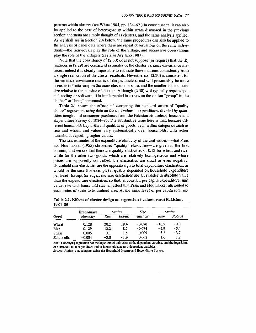
Table 2.1 shows the effects of correcting the standard errors of "qualitychoice" regressions using data on the unit values-expenditures divided by quan-tities bought-of consumer purchases from the Pakistan Household Income andExpenditure Survey of 1984-85. The substantive issue here is that, because dif-ferent households buy different qualities of goods, even within categories such asrice and wheat, unit values vary systematically over households, with richerhouseholds reporting higher values.
The OLS estimates of the expenditure elasticity of the unit values-what Praisand Houthakker (1955) christened "quality" elasticities-are given in the firstcolumn, and we see that there are quality elasticities of 0.13 for wheat and rice,while for the other two goods, which are relatively homogeneous and whoseprices are supposedly controlled, the elasticities are small or even negative.Household size elasticities are the opposite sign to total expenditure elasticities, aswould be the case (for example) if quality depended on household expenditureper head. Except for sugar, the size elasticities are all smaller in absolute valuethan the expenditure elasticities, so that, at constant per capita expenditure, unitvalues rise with household size, an effect that Prais and Houthakker attributed toeconomies of scale to household size. At the same level of per capita total ex-
Table 2.1. Effects of cluster design on regression t-values, rural Pakistan,1984-85
Expenditure t-value Size t-valueGood elasticity Raw Robust elasticity Raw Robust
Wheat 0.128 20.2 18.4 -0.070 -10.5 -9.0Rice 0.129 12.2 8.7 -0.074 -6.9 -5.4Sugar 0.005 3.1 1.5 -0.009 -5.2 -3.7Edible oils -0.004 -3.0 -1.9 0.002 1.6 1.2Note: Underlying regression has the logarithm of unit value as the dependent variable, and the logarithmsof household total expenditure and of household size as independent variables.Source: Author's calculations using the Household Income and Expenditure Survey.

78 THE ANALYSIS OF HOUSEHOLD SURVEYS
penditure, larger households are better-off than smaller households and, in con-sequence, buy better-quality foods. The robust t-values are smaller than theuncorrected values, although as suggested by the theoretical results, the ratios ofthe adjusted to unadjusted values are a good deal smaller than the (square roots ofthe) design effects. Even so, the reductions in the t-values for the estimated qua-lity elasticities for sugar and edible oils are substantial. Without correction, wewould almost certainly (mistakenly) reject the hypothesis that the quality elastici-ties for these two goods are zero; after correction, the t-values come within therange of acceptance.
2.3 Heteroskedasticity and quantile regressions
As we shall see in the next chapter, when we come to look at the distributionsover households of the various components of living standards-income, con-sumption of various goods and their aggregate-it is rare to find variables that arenormally distributed, even after standard transformations like taking logarithms orforming ratios. The large numbers of observations in many surveys permit us tolook at the distributional assumptions that go into standard regression analysis,and even after transformation it is rarely possible to justify the textbook assump-tions that, conditional on the independent variables, the dependent variables areindependently, identically, and normally distributed. The previous section dis-cussed how a cluster survey design is likely to lead to a violation of conditionalindependence. In this section, I turn to the "identically distributed" assumption,and consider the consequences of heteroskedasticity. Just as lack of independenceappears to be the rule rather than the exception, so does heteroskedasticity seemto be almost always present in survey data.
The first subsection looks at linear regression models, at the reasons for het-eroskedasticity, and at its consequences. I suggest that the computation of quan-tile regressions is useful, both in its own right, because quantile regression esti-mates will often have better properties than OLS, as a way of assessing the hetero-skedasticity in the conditional distribution of the variable of interest, and as astepping stone to the nonparametric methods discussed in the next two chapters.As was the case for clustering, a consequence of heteroskedasticity in regressionanalysis is to invalidate the usual formulas for the calculation of standard errors,and as with clustering, there exists a straightforward correction procedure.
Matters are much less simple when we move from regressions to models withlimited dependent variables. In regression analysis, the estimation of scale param-eters can be separated from the estimation of location parameters, but the separa-tion breaks down in probits, logits, Tobits, and in sample selectivity models. Iillustrate some of the difficulties using the Tobit model, and provide a simple butrealistic example of censoring at zero where the application of maximum-likeli-hood Tobit techniques-something that is nowadays quite routine in the develop-ment literature-can lead to estimates that are no better than OLS. There are cur-rently no straightforward solutions to these difficulties, but I review some of theoptions and make some suggestions for practice.

ECONOMETRIC ISSUES FOR SURVEY DATA 79
Heteroskedasticity in regression analysis
It is a fact that regression functions estimated from survey data are typically nothomoskedastic. Why this should be is of secondary importance; indeed it is just asreasonable to ask why it should be supposed that conditional expectations shouldbe homoskedastic. Nevertheless, we have already seen in Section 2.1 above thateven when individual behavior generates homoskedastic regression functionswithin strata or villages, but there is heterogeneity between villages, there will beheteroskedasticity in the overall regression function. Similar results apply to het-erogeneity at the individual level. If the response coefficients , differ by house-hold, and we treat them as random, we may write
(2.31) E(y;ixi,Pi) = 1x2; V(yix1,,id = a-2
Suppose that the ,Bi have mean P and variance-covariance matrix Q, then (2.31)generates the heteroskedastic regression model
(2.32) E(yi1xi) = P'xi; V(yiIxi) = o2 +x'Qx .
Models like (2.32) motivate the standard test procedures for heteroskedasticitysuch as the Breusch-Pagan (1979) test, or White's (1980) information matrix test(see also Chesher 1984 for the link with individual heterogeneity.) The Breusch-Pagan test is particularly straightforward to implement. The OLS residuals fromthe regression with suspected heteroskedasticity are first normalized by divisionby the estimated standard error of the equation. Their squares are then regressedon the variables thought to be generating the heteroskedasticity-if (2.32) iscorrect, these should include the original x-variables, their squares, and cross-pro-ducts-and half the explained sum of squares tested against the x2 distributionwith degrees of freedom equal to the number of variables in this supplementaryregression.
In the presence of heteroskedasticity, OLS is inefficient and the usual formulasfor standard errors are incorrect. In cases where efficiency is not a prime concern,we may nevertheless want to use the OLS estimates, but to correct the standarderrors. This can be done exactly as in (2.30) above, a formula that is robust to thepresence of both heteroskedasticity and cluster effects. If there are no clusters,(2.30) can be applied by treating each household as its own cluster so that thereare no cross-effects within clusters and the formula can be written
(2.33) V(o) = (X'X)'- (E ei2xixi/') (X 'X)-l
where xi is the column vector of explanatory variables for household i and ei2 isthe squared residual from the OLS regression. This formula, which comes origin-ally from Eicker (1967) and Huber (1967), was introduced into econometrics byWhite (1980). Its performance in finite samples can be improved by a number ofpossible corrections; the simplest requires that e 2 in (2.33) be multiplied by

80 THE ANALYSIS OF HOUSEHOLD SURVEYS
(n - k)Y'n, where k is the number of regressors and n the sample size, see David-son and MacKinnon (1993, 552-56.) In practice, the heteroskedasticity correctionto the variance-covariance matrix (2.33) is usually quantitatively less importantthan the correction for intracluster correlations, (2.30).
Quantile regressions
The presence of heteroskedasticity can be conveniently analyzed and displayed byestimating quantile regressions following the original proposals by Koenker andBassett (1978, 1982). To see how these work, it is convenient to start from thestandard homoskedastic regression model.
Figure 2.1 illustrates quantiles in the (standard) case where heteroskedasticityis absent. The regression line a + Px is the expectation of y conditional on x, andthe three "humped" curves schematically illustrate the conditional densities of theerrors given x; in principle, these densities should rise perpendicularly from thepage. For each value of x, consider a process whereby we mark the percentiles ofthe conditional distribution, and then connect up the same percentiles for differentvalues of x. If the distribution of errors is symmetrical, as shown in Figure 2.1, theconditional mean, or regression function, will be at the 50th percentile or median,so that joining up the conditional medians simply reproduces the regression. Whenthe distribution of errors is also homoskedastic, the percentiles will always be atthe same distance from the median, no matter what the value of x. Figure 2.1shows the lines formed by joining the points corresponding to the 10th and 90th
Figure 2.1. Schematic figure of a homoskedastic linear regression function
90th~~~~~~~~~~~It percentile
Note: The solid line shows the regression function of y on x, assumed to be linear. The broken linesshow the 10th and 90th percentiles of the distribution of y conditional on x.

ECONOMETRIC ISSUES FOR SURVEY DATA 81
percentiles of the conditional distributions. Because the regression is homoske-dastic, these are straight lines that are parallel to, and equidistant from, the regres-sion line.
When regressions are heteroskedastic, or when the errors are asymmetric,marking and joining up percentiles will give quite different results. If the residualsare symmetric but heteroskedastic, the distance of each percentile from the regres-sion line will be different at different values of x. Joining up the percentiles fordifferent values of x will not necessarily lead to straight lines or to any other sim-ple curve. However, we can stillfit straight lines to the percentiles, and it is thisthat is accomplished by quantile regression. If the heteroskedasticity is linked tothe value of x, with the distribution of residuals becoming more or less dispersedas x becomes larger, then the quantile regressions for percentiles other than themedian will no longer be parallel to the regression line, but will diverge from it (orconverge to it) for larger values of x.
Figure 2.2 illustrates using a food Engel curve for the rural data from the1984-85 Household Income and Expenditure Survey of Pakistan. Previous experi-ence has shown that the budget share devoted to food can often be well approxi-mated as a linear function of the logarithm of household expenditure per capita, asfirst proposed by Working (1943). The points in the figure are a 10 percent ran-dom sample of the 9,119 households in the survey whose logarithm of per capitaexpenditure lies between 3 and 8; a small number of households at the extremes ofthe distribution are thereby excluded from the figure, but not from the calcula-
Figure 2.2. Scatter diagram and quantile regressions for food shareand total expenditure, Pakistan, 1984-85
90th percentile
0.8 i
0
0.4-
0.2
10th percentile
0.0.4-
II I I I
3 4 5 6 7 8Logarithm of household expenditure per head
Note: The scatter as shown is a ten percent random sample of the points used in the regressions. Theregression lines shown were obtained using the 'qreg' command in STATA and correspond to the 10th,50th, and 90th percentiles.Source: Author's calculations based on Household Income and Expenditure Survey.

82 THE ANALYSIS OF HOUSEHOLD SURVEYS
tions. The three lines in the figure are the quantile regressions corresponding tothe 10th, 50th, and 90th percentiles of the distribution of the food share condi-tional on the logarithm of household expenditure per head; these were calculatedusing all 9,119 households. The procedures for estimating these regressions,calculated using the "qreg" command in STATA, are discussed in the technicalnote that follows, but the principle should be clear from the foregoing discussion.
The slopes of the three lines differ; the median regression (50th percentile) hasa slope of -0.094 (the OLS slope is -0.091), while the lower line has slope -0.121,and the upper -0.054. These differences and the widening spread between thelines as we move to the right show the increase in the conditional variance of theregression among better-off households; the 10th and 90th percentiles of the con-ditional distribution are much further apart among richer than poorer households.Those with more to spend in total devote a good deal less of their budgets to food,but there is also more dispersion of tastes among them.
Quantile regressions are not only useful for discovering heteroskedasticity. Bycalculating regressions for different quantiles, it is possible to explore the shapeof the conditional distribution, something that is often of interest in its own right,even when heteroskedasticity is not the immediate cause for concern. A verysimple example is shown in Figure 2.3, which illustrates age profiles of earningsfor black and white workers from the 1993 South African Living Standards Sur-vey. Earnings are monthly earnings in the "regular" sector, and the graphs use
Figure 2.3. Quantile regressions of the logarithm of earnings on age by race,South Africa, 1993(log of rand per month)
Blacks Whites9 9
8 /= =""\ 80hecni
X0thh peentile
20 60 4 0 6 0 2 0 4 50t 60 701
10kh perodctl
05 5
4 ~~~~4 _ _ _ _ _ _ _ _
20 30 40 50 60 70' 20 310 40 50 60 70
Age
Source: Authoes calculations using the South African Living Standards Survey, 1993.

ECONOMETRIC ISSUES FOR SURVEY DATA 83
only data for those workers who report such earnings. The two panels show thequantile regressions of the logarithm of earnings on age and age squared for the10th, 50th, and 90th percentiles for Black and White workers separately. The useof a quadratic in age restricts the shapes of the profiles, but allows them to differby race and by percentile, as in fact they do. The curves show not only the vastdifferences in earnings between Blacks and Whites-a difference in logarithms of1 is a ratio difference of more than 2.7-but also that the shapes of the age pro-files are different. Those whose earnings are at the top within their age group arethe more highly-educated workers in more highly-skilled jobs, and because thehuman capital required for these jobs takes time to accumulate, the profile at the90th percentile for whites has a stronger hump-shape than do the profiles for the50th and 10th percentiles. There is no corresponding phenomenon for Blacks,presumably because, in South Africa in 1993, even the most able Blacks are res-tricted in their access to education and to high-skill jobs. These graphs and theunderlying regressions do not tell us anything about the causal processes thatgenerate the differences, but they present the data in an interesting way that canbe suggestive of ideas for a deeper investigation (see Mwabu and Schultz 1995for more formal analysis of earnings in South Africa, Mwabu and Schultz 1996for a use of quantile regression in the same context, and Buchinsky 1994 for theuse of quantile regressions to describe the wage structure in the U.S.)
There are also arguments for preferring the parameters of the median regres-sion to those from the OLS regression. Even given the Gauss-Markov assumptionsof homoskedasticity and independence, least squares is only efficient within the(restrictive) class of linear, unbiased estimators, although if the conditional distri-bution is normal, OLS will be minimum variance among the broader class of allunbiased estimators. When the distribution of residuals is not normal, there willusually exist nonlinear (and/or biased) estimators that are more efficient than OLS,and quantile regressions will sometimes be among them. In particular, the medianregression is more resistant to outliers than is OLS, a major advantage in workingwith large-scale survey data.
*Technical note: calculating quantile regressions
In the past, the applicability of quantile regression techniques has been limited,not because they are inherently unattractive, but by computational difficulties.These have now been resolved. Just as in calculating the median itself, medianregression can be defined by minimizing the absolute sum of the errors ratherthan, as in least squares, by minimizing the sum of their squares. It is thus alsoknown as the LAD estimator, for Least Absolute Deviations. Hence, the medianregression coefficients can be obtained by minimizing 4 given by
n n
(2.34) = Elyi _XiPI = (y 1 -xi,)sgn(yi-x /)i=l i=1
where sgn(a) is the sign of a, 1 if a is positive, and -1 if a is negative or zero. (Ihave reverted to the standard use of n for the sample size, since there is no longer
84 THE ANALYSIS OF HOUSEHOLD SURVEYS
a need to separate the number of clusters from the total number of observations.)The intuition for why (2.34) works comes from thinking about the first-order con-dition that is satisfied by the parameters that minimize (2.34), which is, forj = l, ..,k, n
(2.35) Exijsgn(y i x)) = 0.i=1
Note first that if there is only a constant in the regression, (2.35) says that the con-stant should be chosen so that there are an equal number of points on either sideof it, which defines the median. Second, note the similarity between (2.35) andthe OLS first-order conditions, which are identical except for the "sgn" function;in median regression, it is only the sign of each residual that counts, whereas inOLS it is its magnitude.
Quantile regressions other than median can be defined by minimizing, not(2.34), but
q = -(1-q) S (yi-x/P) + q E (yi-x,i/)
(2.36) y•xP y>x/p
= E [q-l(yS,•xiPA)](yi -x'i)i=1
where O<q<l is the quantile of interest, and the value of the function l(z) signalsthe truth (1) or otherwise (0) of the statement z. The minimization conditioncorresponding to (2.35) is now
(2.37) Exij[q - 1(yi <xP)] = 0
which is clearly equivalent to (2.35) when q is a half. Once again, note that if theregression contains only a constant term, the constant is set so that lOOq percentof the sample points are below it, and 100(1 - q) percent above.
The computation of quantile estimators is eased by the recognition that theminimization of (2.36) can be accomplished by linear programming, so that evenfor large data sets, the calculations are not burdensome. The same cannot be saidfor the estimation of the variance-covariance matrix of the parameter estimates.When the residuals are homoskedastic, there is an asymptotic formula providedby Koenker and Bassett (1982) that gives the variance-covariance matrix of theparameters as the usual (XIX)-i matrix scaled by a quantity that depends (in-versely) on the density of the errors at the quantiles of interest. Estimation of thisdensity is not straightforward, but more seriously, the formula appears to givevery poor results-typically gross underestimation of standard errors-in thepresence of heteroskedasticity, which is often the reason for using quantile reg-ression in the first place!
It is therefore important to use some other method for estimating standarderrors, such as the bootstrap, a version of which is implemented in the "bsqreg"command in STATA, whose manual, Stata Corporation (1993, Vol. 3, 96-106)provides a useful description of quantile regressions in general. (Note that theSTATA version does not allow for clustering but it is straightforward, if time-con-
ECONOMETRIC ISSUES FOR SURVEY DATA 85
suming, to bootstrap quantile regressions using the clustered bootstrap illustratedin Example 1.3 in the Code Appendix.)
Heteroskedasticity and limited dependent variable models
In regression analysis, the presence of heteroskedasticity and nonnormality isproblematic because of potential efficiency losses, and because of the need tocorrect the usual formulas for standard errors. However, regression analysis issomewhat of a special case because the estimation of parameters of location-theconditional mean or conditional median-is independent of the estimation ofscale-the dispersion around the conditional location. In limited dependent vari-able models, scale and location are intimately bound together, and as a result,misspecification of scale can lead to inconsistency in estimates of location.
Probit and logit models provide perhaps the clearest examples of the difficul-ties that arise. There is a dependent variable yi which is either 1 or 0 according towhether or not an unobserved or latent variable y' is positive or nonpositive. Thelatent variable is defined by analogy to a regression model,
(2.38) yi = f(xi) + ui, E(u;) = 0, E(ui2) = a2[ g(Zi)12
where x and z are vectors of variables controlling the "regression" and the "hete-roskedasticity" respectively, and f (.) and g (.) are functions, the former usuallyassumed to be known, the latter unknown. Suppose that F(.) is the cumulativedistribution function (CDF) of the standardized residual u,/ag (zi), and that F(.)is symmetric around 0 so that F(a) = 1 - F( -a), then
(2.39) Pi = Prob(y, = 1) = F[f(x 1 )/ag(z,)].
If we know the function F(.), which is in itself assuming a great deal, then givendata on y, x, and z, the model gives no more information on which to base estima-tion than is contained in the probabilities (2.39). But by inspection of (2.39) it isimmediately clear that it is not possible to separate the "heteroskedasticity" func-tion g (z) from the "regression" function f( x). For example, suppose that f( x)has the standard linear specification x '13, that the elements of z are the same asthose of x, and that it so happens that g(z) = g(x) =x'13/x'y. Then the applica-tion of maximum-likelihood estimation (MLE) will yield estimates that are con-sistent, not for 1, but for y! The latent-variable or regression approach to dicho-tomous models can be misleading if we treat it too seriously; we observe l's orO's, and we can use them to model the probabilities, but that is all.
The point of the previous paragraph is so obvious and so well understood thatit is hardly of practical importance; the confounding of heteroskedasticity and"structure" is unlikely to lead to problems of interpretation. It is standard proce-dure in estimating dichotomous models to set the variance in (2.38) to be unity,and since it is clear that all that can be estimated is the effects of the covariates onthe probability, it will usually be of no importance whether the mechanism works

86 THE ANALYSIS OF HOUSEHOLD SURVEYS
through the mean or the variance of the latent "regression" (2.38). While it iscorrect to say that probit or logit is inconsistent under heteroskedasticity, theinconsistency would only be a problem if the parameters of the function f werethe parameters of interest. These parameters are identified only by the homoske-dasticity assumption, so that the inconsistency result is both trivial and obvious.(It is perhaps worth noting that STATA has "hlogit" and "hprobit" commands forlogit and probit that match the "hreg" command for regression. But these shouldnot be used to correct standard errors in logit and probit; rather they should beused to correct standard errors for clustering, so that the analogy is with (2.30),not (2.33).)
Related but more serious difficulties occur with heteroskedasticity when ana-lyzing censored regression models, truncated regressions, or regressions with se-lectivity, where the inconsistencies are a good deal more troublesome. I illustrateusing the censored regression model, or Tobit-after Tobin's (1958) probit-because the model is directly relevant to the analysis in later chapters, and be-cause the technique is widely used in the development literature. Consider inparticular the demand for a good, which can be purchased only in positive quanti-ties. If there were no such restriction, we might postulate a linear regression of theform(2.40) Yi =x,$ + ui.
When y,* is positive, everything is as usual and actual demand y1 is equal to y,*.But negative values of yi* are "censored" and replaced by zero, the minimumallowed. The model for the observed yi can thus be written as
(2.41) yi = max(0, x' + ui ).
I note in passing that the model can be derived more elegantly as in Heckman(1974), who considers a labor supply example, and shows that (2.41) is consistentwith choice theory when hours worked cannot be negative.
The left-hand panel of Figure 2.4 shows a simulation of an example of a stand-ard Tobit model. The latent variable is given by x, - 40 + ui with the x's takingthe 100 values from 1 to 100, and the u's randomly and independently drawnfrom a normal distribution with mean zero and standard deviation 20. The smallcircles on the graph show the resulting scatter of y, against xi. Because of thecensoring, which is more severe for low values of the explanatory variable, theOLS regression line has a slope less than one; in 100 replications the OLS estimatorhad a mean of 0.637 with a standard deviation of 0.055, so that the bias shown inthe figure for one particular realization is typical of this situation. A better methodis to follow Tobin, and maximize the log-likelihood function
InL = _-t (Ina + ln21) - ...LE(Y. -x,$)22 20_,,
(2.42) +Ei (xl

ECONOMETRIC ISSUES FOR SURVEY DATA 87
where n+ is the number of strictly positive observations, i, and io indicate thatthe respective sums are taken over positive and zero observations, respectively,and 1 is the c.d.f. of the standard normal distribution. The first two terms on theright-hand side of (2.42) are exactly those that would appear in the likelihoodfunction of a standard normal regression, and would be the only terms to appearin the absence of censoring. The final term comes from the observations that arecensored to zero; for each such observation we do not observe the exact value ofthe latent variable, only that it is zero or less, so that the contribution to the loglikelihood is the logarithm of the probability of that event. Estimates of ,3 and aare obtained by maximizing (2.42), a nonlinear problem whose solution is guar-anteed by the fact the log-likelihood function is convex in the parameters, and sohas a unique maximum. This maximum-likelihood technique works well for theleft-hand panel of the figure; in the 100 replications, the Tobit estimates of theslope averaged 1.009 with a standard deviation of 0.100. In this case, where thenormality assumption is correct, and the disturbances homoskedastic, maximumlikelihood overcomes the inconsistency of OLS.
That all will not be as well in the presence of heteroskedasticity can be seenfrom the likelihood function (2.42) where the last term, which is the contributionto the likelihood of the censored observations, contains both the scale and loca-tion parameters. The standard noncensored likelihood function, which is (2.42)without the last term, has the property that the derivatives of the log-likelihoodfunction with respect to the P's are independent of a, at least in expectation, andvice versa, something that is not true for (2.42). This gives a precise meaning tothe notion that scale and location are independent in the regression model, but
Figure 2.4. Tobit models with and without heteroskedasticity
Without heteroskedasticity With heteroskedasticity
100 °000
80 0
60 * 04a OLtregtesoioo v ofr >
> 40 0 00 00.. 0 oLs regression 0
4F 0. oO°, 0H ,ooz°OQ.00 0.00
0 f 0~~~~~0
O) *.. o °~ 0 t 0 o.,'0 a 0 a0.-' 00
Tbbit aE One
0 20 40 60 80 100 0 20 40 60 80 100
Independent variable x
Note: See text for model definition and estimation procedures.Source: Author's calculations.
88 THEANALYSISOFHOUSEHOLDSURVEYS
dependent in these models with limited dependent variables. As a result of thedependence, misspecification of scale will cause the P's that maximize (2.42) tobe inconsistent for the true parameters, a result first noted by Hurd (1979), Nelson(1981), and Arabmazar and Schmidt (1981).
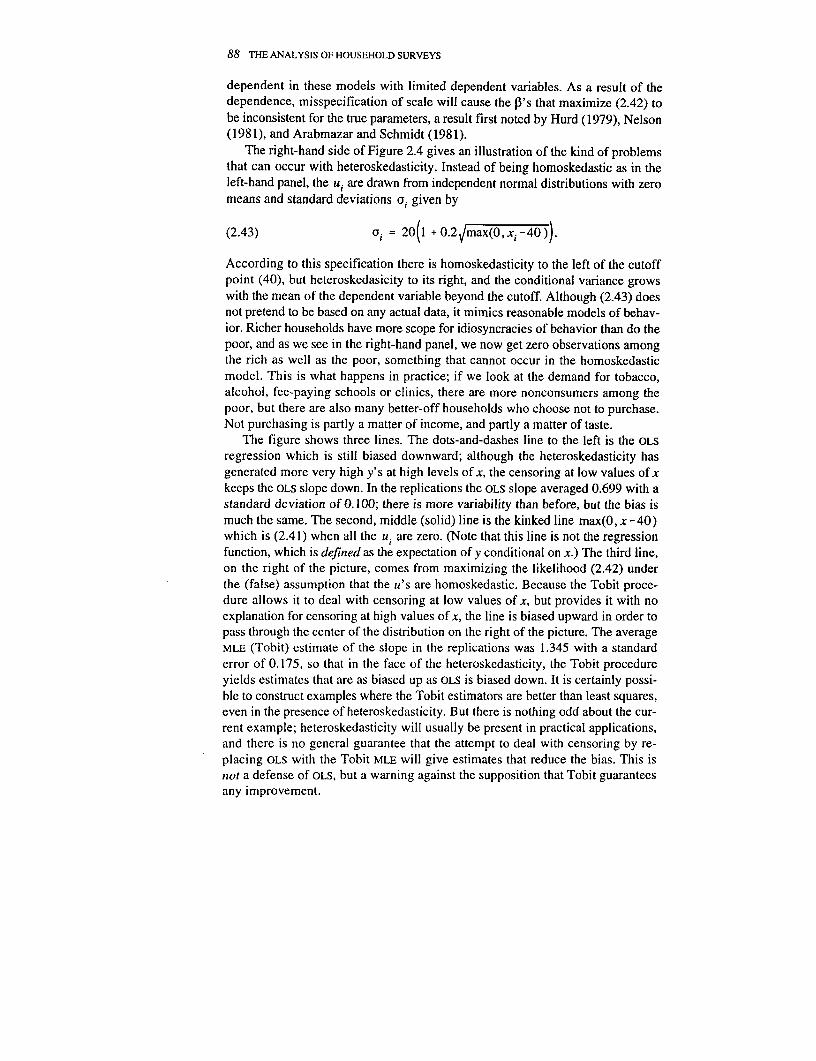
The right-hand side of Figure 2.4 gives an illustration of the kind of problemsthat can occur with heteroskedasticity. Instead of being homoskedastic as in theleft-hand panel, the ui are drawn from independent normal distributions with zeromeans and standard deviations a, given by
(2.43) °i = 20(1 +0.2 nmax(0,xi- 40 )).
According to this specification there is homoskedasticity to the left of the cutoffpoint (40), but heteroskedasicity to its right, and the conditional variance growswith the mean of the dependent variable beyond the cutoff. Although (2.43) doesnot pretend to be based on any actual data, it mimics reasonable models of behav-ior. Richer households have more scope for idiosyncracies of behavior than do thepoor, and as we see in the right-hand panel, we now get zero observations amongthe rich as well as the poor, something that cannot occur in the homoskedasticmodel. This is what happens in practice; if we look at the demand for tobacco,alcohol, fee-paying schools or clinics, there are more nonconsumers among thepoor, but there are also many better-off households who choose not to purchase.Not purchasing is partly a matter of income, and partly a matter of taste.
The figure shows three lines. The dots-and-dashes line to the left is the OLS
regression which is still biased downward; although the heteroskedasticity hasgenerated more very high y's at high levels of x, the censoring at low values of xkeeps the OLS slope down. In the replications the OLS slope averaged 0.699 with astandard deviation of 0.100; there is more variability than before, but the bias ismuch the same. The second, middle (solid) line is the kinked line max(0, x - 40)which is (2.41) when all the ui are zero. (Note that this line is not the regressionfunction, which is defined as the expectation of y conditional on x.) The third line,on the right of the picture, comes from maximizing the likelihood (2.42) underthe (false) assumption that the u's are homoskedastic. Because the Tobit proce-dure allows it to deal with censoring at low values of x, but provides it with noexplanation for censoring at high values of x, the line is biased upward in order topass through the center of the distribution on the right of the picture. The averageMLE (Tobit) estimate of the slope in the replications was 1.345 with a standarderror of 0.175, so that in the face of the heteroskedasticity, the Tobit procedureyields estimates that are as biased up as OLS is biased down. It is certainly possi-ble to construct examples where the Tobit estimators are better than least squares,even in the presence of heteroskedasticity. But there is nothing odd about the cur-rent example; heteroskedasticity will usually be present in practical applications,and there is no general guarantee that the attempt to deal with censoring by re-placing OLS with the Tobit MLE will give estimates that reduce the bias. This isnot a defense of OLS, but a warning against the supposition that Tobit guaranteesany improvement.

ECONOMETRIC ISSUES FOR SURVEY DATA 89
In practice, the situation is worse than in this example. Even when there is noheteroskedasticity, the consistency of the Tobit estimates requires that the distri-bution of errors be normal, and biases can occur when it is not (see Goldberger1983 and Arabmazar and Schmidt 1982). And since the distribution of the u's isalmost always unknown, it is unclear how one might respecify the likelihoodfunction in order to do better. Even so, censored data occur frequently in practice,and we need some method for estimating sensible models. There are two very dif-ferent approaches; the first is to look for estimation strategies that are robustagainst heteroskedasticity of the u's in (2.41) and that require only weak assump-tions about their distribution, while the second is more radical, and essentiallyabandons the Tobit approach altogether. I begin with the former.
*Robust estimation of censored regression models
There are a number of different estimators that implement the first approach,yielding nonparametric Tobit estimators-nonparametric referring to the distribu-tion of the u's, not to the functional form of the latent variable which remainslinear. None of these has yet passed into standard usage, and I review only one,Powell's (1984) censored LAD estimator. It is relatively easily implemented andappears to work in practice. (An alternative is Powell's (1986) symmetricallytrimmed least squares estimator.)
One of the most useful properties of quantiles is that they are preserved undermonotone transformations; for example, if we have a set of positive observations,and we take logarithms, the median of the logarithms will be the logarithm of themedian of the untransformed data. Since max(O, z) is monotone nondecreasing inz, we can take medians of (2.41) conditional on xi to get
(2.44) q50(yilxi) = max[0,q50(x,'f +uiIxi)] = max(0,x1x/)
where q50(. Ix) denotes the median of the distribution coniditional on x and themedian of u, is assumed to be 0. But as we have already seen, LAD regressionestimates the conditional median regression, so that J3 can be consistently esti-mated by the parameter vector that minimizes
n
(2.45) Y I yi - max(0, x,i ) Ii=l
which is what Powell suggests. The consistency of this estimator does not requireknowledge of the distribution of the u's, nor is it assumed that the distribution ishomoskedastic, only that it has median 0.
Although Powell's estimator is not available in standard software, it can becalculated from repeated application of median regression following a suggestionof Buchinsky (1994, p. 412). The first regression is run on all the observations,and the predicted values x,'f calculated; these are used to discard sample observa-tions where the predicted values are negative. The median regression is then re-peated on the truncated sample, the parameter estimates used to recalculate x,/f
90 THE ANALYSIS OF HOUSEHOLD SURVEYS
for the whole sample, the negative values discarded, and so on until convergence.In (occasional) cases where the procedure does not converge, but cycles througha finite set of parameters, the parameters with the highest value of the criterionfunction should be chosen. Standard errors can be taken from the final iterationthough, as before, bootstrapped estimates should be used.
Such a procedure is easily coded in STATA, and was applied to the heteroske-dastic example given above and shown in Figure 2.4 (see Example 2.1 in theCode Appendix). To simplify the coding, the procedure was terminated after 10median regressions, so that to the extent that convergence had not been attained,the results will be biased against Powell's estimator. On average, the method doeswell, and the mean of the censored LAD estimator over the 100 replications was0.946. However, there is a price to be paid in variance, and the standard deviationof 0.305 is three times that of the OLS estimator and more than one and a halftimes larger than that of the Tobit. As a result, and although both Tobit and OLS
are inconsistent, in only 55 out of 100 of the replications is the censored LAD
closer to the truth than both OLS and Tobit. Of course, the bias to variance trade-off turns in favor of Powell's estimator as the sample size becomes larger. With1,000 observations instead of 100, and with the new x values again equally spacedbut 10 times closer, the censored LAD estimator is closer to the truth than eitherOLS or Tobit in 96 percent of the cases. Since most household surveys will havesample sizes at least this large, Powell's estimator is worth serious consideration.At the very least, comparing it with the Tobit estimates will provide a usefulguide to failure of homoskedasticity or normality (see Newey 1987 for an exer-cise of this kind).
Even so, the censored LAD estimator is designed for the censored regressionmodel, and does not apply to other cases, such as truncation, where the observa-tions that would have been negative do not appear in the sample instead of beingreplaced by zeros, nor to more general models of sample selectivity. In these, thecensoring or truncation of one variable is determined by the behavior of a secondlatent variable regression, so that
(2.46) Yi1 =Y2i = ZiY + U2N
where u1 and u2 are typically allowed to be correlated, y2i is observed as adichotomous variable indicating whether or not Y" is positive, and yli is observedas yi when Y2, is 1, and is zero otherwise. Equations (2.46) are a generalizationof Tobit, whereby the censoring is controlled by variables that are different fromthe variables that control the magnitude of the variable of interest. If the two setsof u's are assumed to be jointly normally distributed, (2.46) can be estimated bymaximum likelihood, or by Heckman's (1976) two-step estimator-the "Heckit"procedure (see the next section for further discussion). As with Tobit, which is aspecial case, these methods do not yield consistent estimates in the presence ofheteroskedasticity or nonnormality, and as with Tobit, the provision of nonpara-metric estimators is a lively topic of current research in econometrics. I shallreturn to these topics in more detail in the next section.
ECONOMETRIC ISSUES FOR SURVEY DATA 91
Radical approaches to censored regressions
Serious attention must also be given to a second, more radical, approach thatquestions the usefulness of these models in general. There are conceptual issuesas well as practical ones. In the first place, these models are typically presented aselaborations of linear regression, in which a standard regression equation is ex-tended to deal with censoring, truncation, selectivity, or whatever is the issue athand. However, in so doing they make a major break from the standard situationpresented in the introduction where the regressionfunction, the expectation of thedependent variable conditional on the covariates, coincides with the deterministicpart of the regression model. In the Tobit and its generalizations, the regressionfunctions are no longer simple linear functions of the x's, but are more complexexpressions that involve the distribution of the u's. For example, in the censoredregression model (2.41), the regression function is given by
E(yixI) = xi)x3 + E(u Ix,l + u 2 0)
(2.47) x,p + [I-F(-x!l)]f f udF(u)
where F(u) is the CDF of the u's. Absent knowledge of F, this regression functiondoes not even identify the Al's-see Powell (1989)-but more fundamentally, weshould ask how it has come about that we have to deal with such an awkward,difficult, and nonrobust object.
Regressions are routinely assumed to be linear, not because linearity is thoughtto be exactly true, but because it is convenient. A linear model is often a sensiblefirst approximation, and linear regressions are easy to estimate, to replicate, andto interpret. But once we move into models with censoring or selection, it is muchless convenient to start with linearity, since it buys us no simplification. It istherefore worth considering alternative possibilities, such as starting by specifyinga suitable functional form for the regression function itself, rather than for the partof the model that would have been the regression function had we been dealingwith a linear model. Linearity will often not be appropriate for the regressionfunction, but there are many other possibilities, and as we shall see in the nextchapter, it is often possible to finesse the functional form issue altogether. Suchan approach goes beyond partially nonparametric treatments that allow arbitrarydistributional assumptions for the disturbances while maintaining linearity for thefunctional form of the model itself, and recognizes that the functional form is asmuch an unknown as is the error distribution. It also explicitly abandons theattempt to estimate the structure of selectivity or censoring, and focusses on fea-tures of the data-such as regression functions-that are clearly and uncontrover-sially observable. There will sometimes be a cost to abandoning the structure, butthere are many policy problems for which the structure is irrelevant, and whichcan be addressed through the regression function.
A good example is the effect of a change in tax rates on tax revenue. A gov-ernment is considering a reduction in the subsidy on wheat (say), and needs to

92 THE ANALYSIS OF HOUSEHOLD SURvEYS
know the extent to which demand will be reduced at the higher price. The quan-tity of interest is the effect of price on average demand. Suppose that we have sur-vey data on wheat purchases, together with regional or temporal price variation aswell as other relevant explanatory variables. Some households buy positive quan-tities of wheat, and some buy none, a situation that would seem to call for a TobitEstimation of the model yields an estimate of the response of quantity to price forthose who buy wheat. But the policymaker is interested not only in this effect, butalso in the loss of demand from those who previously purchased, but who willdrop out of the market at the higher price. These effects will have to be modeledseparately and added into the calculation. But this is an artificial and unneces-sarily elaborate approach to the problem. The policy question is about the effectof price on average demand, averaged over consumers and nonconsumers alike.But this is exactly what we would estimate if we simply regressed quantity onprice, with zeros and nonzeros included in the regression. In this case, not only isthe regression function more convenient to deal with from an econometric per-spective, it is also what we need to know for policy.
2.4 Structure and regression in nonexperimental data
The regression model is the standard workhorse for the analysis of survey data,and the parameters estimated by regression analysis frequently provide usefulsummaries of the data. Even so, they do not always give us what we want. This isparticularly so when the survey data are a poor substitute for unobtainable experi-mental data. For example, if we want to know the effect of constructing healthclinics, or of expanding schools, or what will happen if a minimum wage orhealth coverage is mandated, we should ideally like to conduct an experiment, inwhich some randomly chosen group is given the "treatment," and the results com-pared with a randomly selected group of controls from whom the treatment iswithheld. The randomization guarantees that there are no differences-observableor unobservable-between the two groups. In consequence, if there is a signifi-cant difference in outcomes, it can only be the effect of the treatment. Althoughthe role of policy experiments has been greatly expanded in recent years (seeGrossman 1994 and Newman, Rawlings, and Gertler 1994), there are many caseswhere experiments are difficult or even impossible, sometimes because of thecost, and sometimes because of the moral and political implications. Instead, wehave to use nonexperimental survey data to look at the differences in behaviorbetween different people, and to try to relate the degree of exposure to the treat-ment to variation in the outcomes in which we are interested. Only under idealconditions will regression analysis give the right answers. In this section, I ex-plore the various difficulties; in the next two sections, I look at two of the mostimportant of the econometric solutions, panel data and the technique of instru-mental variables.
The starting point for a nonexperimental study is often a regression model, inwhich the outcome variable y is related to a set of explanatory variables x. At leastone of the x-variables is the treatment variable, while others are "control" vari-

ECONOMETRIC ISSUES FOR SURVEY DATA 93
ables, included so as to allow for differences in outcomes that are not caused bythe treatment and to allow the treatment effect to be isolated. These variables playthe same role as the control group in an experiment. The error term in the regres-sion captures omitted controls, as well as measurement error in the outcome y,and is assumed to satisfy (2.4), that its expectation conditional on the x's is 0. Inthis setup, the expectation of y conditional on x is ,51x, and the effects of thetreatment and controls can be recovered by estimating P3. The most commonproblem with this procedure is the failure-or at least implausibility-of theassumption that the conditional mean of the error term is zero. If a relevant vari-able is omitted, perhaps because it is unobservable or because data are unavail-able, and if that variable is correlated with any of the included x's, the error willnot be orthogonal to the x's, and the conditional expectation of y will not be ,'x.The regression function no longer coincides with the structure that we are tryingto recover, and estimation of the regression function will not yield the parametersof interest. The failure of the structure and the regression function to coincidehappens for many different reasons, some more obvious than others. In this sec-tion, I consider a number of cases that are important in the analysis of householdsurvey data from developing countries.
Simultaneity, feedback, and unobserved heterogeneity
Simultaneity is a classic argument for a correlation between error terms and ex-planatory variables. If we supplement the regression model (2.3) with anotherequation or equations by which some of the explanatory variables are determinedby factors that include y, then the error term in (2.3) will be correlated with one ormore of the x's and OLS estimates will be biased and inconsistent. The classictextbook examples of simultaneity, the interdependence of supply or demand andprice, and the feedbacks through national income from expenditures to income,are usually thought not to be important for microeconomic data, where the pur-chases of individuals are too small to affect price or to influence their own in-comes through macroeconomic feedbacks. As we shall see, this is not necessarilythe case, especially when there are local village markets. Other forms of simulta-neity are also important in micro data, although the underlying causes often havemore to do with omitted or unobservable variables than with feedbacks throughtime. Four examples illustrate.
Example 1. Price and quantities in local markets
In the analysis of demand using microeconomic data, it is usually assumed thatindividual purchases are too small to affect price, so that the simultaneity betweenprice and aggregate demand can be ignored in the analysis of the microeconomicdata. Examples where this is not the case have been provided by Kennan (1989),and local markets in developing countries provide a related case. Suppose that thedemand function for each individual in each village contains an unobservablevillage-level component, and that, because of poor transportation and lack of an

94 THE ANALYSIS OF HOUSEHOLD SURVEYS
integrated market, supply and demand are equilibriated at the village level. Al-though the village-level component in individual demands may contribute little tothe total variance of demand, the other components will cancel out over the vil-lage as a whole, so that the variation in price across villages is correlated withvillage-level taste for the good. Villages that have a relatively high taste for wheatwill tend to have a relatively high price for wheat, and the correlation can beimportant even when regressions are run using data from individuals or house-holds.
To illustrate, write the demand function in the form
(2.48) Yi = aO f pXiC -TPC + Ui, = aO % pxiC - YPc + ac + Cic
where yic is demand by household i in cluster c, xi, is income or some other indi-vidual variable, pc is the common village price, and u k is the error term. As inprevious modeling of clusters, I assume that uic is the sum of a village term acand an idiosyncratic term ec,i both of which are mean-zero random variables.Suppose that aggregate supply for the village is zc per household, which comesfrom a weather-affected harvest but is unresponsive to price (or to income). Mar-ket clearing implies that
(2.49) ZC = Yc = ao + pC - Ypc + ac
which determines price in terms of the village taste effect, supply, and averagevillage income. Because markets have to clear at the village level, the price ishigher in villages with a higher taste for the commodity. In consequence, the priceon the right-hand side of (2.48) is correlated with the ac component of the errorterm, and OLS estimates will be inconsistent. The inconsistency arises even if thevillage contains many households, each of which has a negligible effect on price.
The bias can be large in this case. To make things simple, assume that , = 0,so that income does not appear in (2.48) nor average income in (2.49). Accordingto the latter, price in village c is
(2.50) PC = Y (ao + aC - Zc).
Write V for the OLS estimate of y obtained by regressing individual householddemands on the price in the village in which the household lives. Provided thattastes are uncorrelated with harvests, it is straightforward to show that
y 2
(2.51) plimy =______22a+a
The price response is biased downwards; in addition to the negative effect ofprice on demand, there is a positive effect from demand to price that comes fromthe effect on both of village-level tastes. The bias will only vanish when the vil-lage taste effects aC are absent, and will be large if the variance of tastes is largerelative to the variance of the harvest.
ECONOMETRIC ISSUES FOR SURVEY DATA 95
Example 2. Farm size andfarm productivity
Consider a model of the determinants of agricultural productivity, and in particu-lar the old question of whether larger or smaller farms are more productive; theobservation of an inverse relationship between farm size and productivity goesback to Chayanov (1925), and has acquired the status of a stylized fact; see Sen(1962) for India and Berry and Cline (1979) for reviews.
To examine the proposition, we might use survey data to regress output perhectare on farm size and on other variables not shown, viz.
(2.52) ln(Qi/Ai) = a + , lnAA + ui
where Qi is farm output, A, is farm size, and the common finding is that f0 < 0,so that small farms are "more productive" than large farms. This might be inter-preted to mean that, compared with hired labor, family labor is of better quality,more safely entrusted with valuable animals or machinery, and needs less moni-toring (see Feder 1985; Otsuka, Chuma, and Hayami 1992; and Johnson andRuttan 1994), or as an optimal response by small farmers to uncertainty (seeSrinivasan 1972). It has also sometimes been interpreted as a sign of inefficiency,and of dualistic labor markets, because in the absence of smoothly operating labormarkets farmers may be forced to work too much on their own farms, pushingtheir marginal productivity below the market wage (see particularly Sen 1966,1975). However, if a relationship like (2.52) is estimated on a cross section offarms, and even if the amount of land is outside the control of the farner, (2.52)is likely to suffer from what are effectively simultaneity problems. Such issueshave the distinction of being among the very first topics studied in the early daysof econometrics (see Marschak and Andrews 1944).
Although it may be reasonable to suppose that the farmer treats his farm sizeas fixed when deciding what to plant and how hard-to work, this does not meanthat Ai is uncorrelated with u, in (2.52). Farm size may not be controlled by thefarmer, but fanns do not get to be the size they are at random. The mechanismdetermining farm size will differ from place to place and time to time, but it isunlikely to be independent of the quality of the land. "Desert" farms that are usedfor low-intensity animal grazing are typically larger than "garden" farms, wherethe land is rich and output per hectare is high. Such a correlation will be presentwhether farms are allocated by the market-low-quality land is cheaper per hect-are so that it is easier for an owner-occupier to buy a large farm-or by state-mandated land schemes-each farmer is given a plot large enough to make aliving. In consequence, the right-hand side of (2.52) is at least partly determinedby the left-hand side, and regression estimates of ,5 will be biased downward.
We can also give this simultaneity an omitted variable interpretation whereland quality is the missing variable; if quality could be included in the regressioninstead of in the residual, the new residual could more plausibly be treated asorthogonal to farm size. At the same time, the coefficient f3 would more nearlymeasure the effect of land size, and not as in (2.52) the effect of land size contam-
96 THE ANALYSIS OF HOUSEHOLD SURVEYS
inated by the (negative) projection of land quality on farm size. Indeed, when dataare available on land quality-Bhalla and Roy (1988)-or when quality is con-trolled by iv methods-Benjamin (1993)-there is little or no evidence of a nega-tive relationship between farm size and productivity.
The effect of an omitted variable is worth recording explicitly, since the for-mula is one of the most useful in the econometrician's toolbox, and is routinelyused to assess results and to calculate the direction of bias caused by the omission.Suppose that the correct model is
(2.53) Yi = a + pxi + yzi + ui
and that we have data on y and x, but not on z. In the current example, y is yield,and z is land quality. If we run the regression of y on x, the probability limit of theOLS estimate of P is
(2.54) plim = + y cov(x,Z)var x
In the example, it might be the case that , = 0, so that farm size has no effect onyields conditional on land quality. But y >0, because better land has higheryields, and the probability limit of f3 will be negative because farm size and landquality are negatively correlated.
The land quality problem arises in a similar form if we attempt to use equa-tions like (2.52) to measure the effects on output of extension services or "mod-ern" inputs such as chemical fertilizer. Several studies, Bevan, Collier and Gun-ning (1989) for Kenya and Tanzania, and Deaton and Benjamin (1988) for C6ted'Ivoire, find that a regression of output on fertilizer input shows extremely highreturns, estimates that, if correct, imply considerable inefficiency and scope forgovernment intervention.
Deaton and Benjamin use the 1985 Living Standards Survey of C6te d'Ivoireto estimate the following regression between cocoa output, the structure of theorchard, and the use of fertilizer and insecticide,
ln(Q ILM) = 5.621 + 0.526 (LO ILM) + 0.0541nsect
(2.55) (68.5) (4.3) (2.5)(2.55) + 0.158 Fert
(2.8)
where Q is kilos of cocoa produced on the farm, LM and LO are the numbers ofhectares of "mature" and "old" trees, respectively, and Insect and Fert are ex-penditures in thousands of Central African francs per cocoa hectare on insecticideand fertilizer, respectively. According to (2.55), an additional 1,000 francs spenton fertilizer will increase the logarithm of output per hectare by 0.158, which at asample mean log yield of 5.64 implies an additional 48 kilos of cocoa at 400francs per kilo, or an additional 19,200 francs. However, only slightly more thana half of the cocoa stands are fully mature, and the farmers pay the mettayeurswho harvest the crop between a half and a third of the total. But even after these

ECONOMETRIC ISSUES FOR SURVEY DATA 97
adjustments, the farmer will be left with a return of 5,400 for an outlay of 1,000francs. Insecticide is estimated to be somewhat less profitable, and the same cal-culation gives a return of only 1,800 for each 1,000 francs outlay. Yet only 1 in14 farmers uses fertilizer, and 1 in 5 uses insecticide.
On the surface, these results seem to indicate very large inefficiencies. How-ever, there are other interpretations. It is likely that highly productive farms aremore likely to adopt fertilizer, particularly if the use of fertilizer is an indicator offarmer quality and the general willingness to adopt modern methods, high-yield-ing varieties, and so on. Credit for fertilizer purchases may only be available tobetter, or to better-off farmers. Suppose also that some farmers cannot use fertil-izer because of local climatic or soil conditions or because the type of trees intheir stand, while others have the conditions to make good use of it. When wecompare these different farms, we shall find what we have found, that farmersthat use fertilizer are more productive, but there is no implication that more fertil-izer should be used. Expenditure on fertilizer in (2.55) may do no more thanindicate that the orchard contains new hybrid varieties of cocoa trees, somethingon which the survey did not collect data.
Example 3. The evaluation of projects
Analysis of the effectiveness of government programs and projects has alwaysbeen a central topic in development economics. Regression analysis seems like ahelpful tool in this endeavor, because it enables us to link outcomes-incomes,consumption, employment, health, fertility-to the presence or extent of pro-grams designed to influence them. The econometric problems of such analysesare similar to those we encountered when linking farm outputs to farm inputs. Inparticular, it is usually impossible to maintain that the explanatory variables-inthis case the programs-are uncorrelated with the regression residuals. Govern-ment programs are not typically run as experiments, in which some randomlyselected groups are treated and others are left alone.
A regression analysis may show that health outcomes are better in areas wherethe government has put clinics, but such an analysis takes no account of the pro-cess whereby sites are chosen. Clinics may be put where health outcomes werepreviously very poor, so that the cross-section regression will tend to underesti-mate their effects, or they may be allocated to relatively wealthy districts that arepolitically powerful, in which case regression analysis will tend to overstate theirtrue impact. Rosenzweig and Wolpin (1986) found evidence of underestimationin the Philippines, where the positive effect of clinics on children's health did notshow up in a cross section of children because clinics were allocated first to theareas where they were most needed. The clinics were being allocated in a desir-able way, and that fact caused regression analysis to fail to detect the benefits. Inthe next section, I shall follow Rosenzweig and Wolpin and show how panel datacan sometimes be used to circumvent these difficulties. I shall return to the issueof project evaluation later in this section when I come to discuss selection bias,and again in Section 2.6 on IV estimation.

98 THE ANALYSIS OF HOUSEHOLD SURVEYS
Example 4. Simultaneity and lags: nutrition andproductivity
It is important to realize that in cross-section data, simultaneity cannot usually beavoided by using lags to ensure that the right-hand side variables are prior in timeto the left-hand side variables. If x precedes y, then it is reasonable to suppose thaty cannot affect x directly. However, there is often a third variable that affects ytoday as well as x yesterday, and if this variable is omitted from the regression,today's y will contain information that is correlated with yesterday's x. The landquality issue in the previous example can be thought about this way; althoughfarm size is determined before the farmer's input and effort decisions, and beforethey and the weather determine farm output, both output and inputs are affectedby land quality, so that there remains a correlation between output and the prede-ternined variables. As a final example, consider one of the more intractable casesof simultaneity, between nourishment and productivity. If poor people cannotwork because they are malnourished, and they cannot eat because they do notearn enough, poor people are excluded from the labor market and there is persis-tent unemployment and destitution. The theory of this interaction was developedby Mirrlees (1975) and Stiglitz (1976), and it has been argued that such a mecha-nism helps account for destitution in India (Dasgupta 1993) and for the slow paceof premodern development in Europe (Fogel 1994).
People who eat better may be more productive, because they have more en-ergy and work more efficiently, but people who work more efficiently also earnmore, out of which they will spend more on food. Disentangling the effect ofnutrition on wages from the Engel curve for food is difficult, and as emphasizedby Bliss and Stern (1981), it is far from clear that the two effects can ever be -disentangled. One possibility, given suitable data, is to suppose that productivitydepends on nutrition with a lag-sustained nutrition is needed for work-whileconsumption depends on current income. Hence, if yt is the productivity of indi-vidual i at time t, and cit is consumption of calories, we might write
(2.56) Yit ~ l= 1 + pici-+ +YZli, +lit
cit = a 2 + P2+ Y2Z2it+ U2 it
where Zt and Z2 are other variables needed to identify the system. Provided equa-tion (2.56) is correct and the two error terms are serially independent, both equa-tions can consistently be estimated by least squares in a cross section with infor-mation on lagged consumption. However, any form of serial dependence in theresiduals ulit will make OLS estimates of the first equation inconsistent. But thereis a good reason to suppose that these residuals will be serially correlated, sincepermanent productivity differences across people that are not attributable to nutri-tion or the other variables will add a constant "individual" component to the error.Individuals who are more productive in one period are likely to be more produc-tive in the next, even when we have controlled for their nutrition and other ob-servable covariates. More productive individuals will have higher incomes and

ECONOMETRIC ISSUES FOR SURVEY DATA 99
higher levels of nutrition, not only today but also yesterday, so that the lag in theequation no longer removes the correlation between the error term and the-right-hand-side variable. In a cross section, predetermined variables can rarely be legit-imately treated as exogenous.
Measurement error
Measurement error in survey data is a fact of life, and while it is not always pos-sible to counter its effects, it is always important to realize what those effects arelikely to be, and to beware of inferences that are possibly attributable to, or con-taminated by, measurement error.
The textbook case is the univariate regression model where both the explana-tory and dependent variables are subject to mean-zero errors of measurement.Hence, for the correctly measured variables y and x, we have the linear relation-ship
(2.57) Yi = a + pxi + u
together with the measurement equations
(2.58) x, = xi + C1i ,i = Yi + C2i
where the measurement error is assumed to be orthogonal to the true variables.Faute de mieux, g is regressed on x, and the OLS parameter estimate of , has theprobability limit
(2.59) plim, = Mx + = PIO
where m. is the variance of the unobservable, correctly measured x, and a2 is thevariance of the measurement error in x. Equation (2.59) is the "iron law of econo-metrics," that the OLS estimate of , is biased towards zero, or "attenuated." Thedegree of attenuation is the ratio of signal to combined signal and noise, AX, thereliability ratio. The presence of measurement error in the dependent variabledoes not bias the regression coefficients, because it simply adds to the variance ofthe equation as a whole. Of course, this measurement error, like the measurementerror in x, will decrease the precision with which the parameters are estimated.
Attenuation bias is amplified by the addition of correctly measured explana-tory variables to the bivariate regression (2.57). Suppose we add a vector z to theright-hand side of (2.57), and assume that z is uncorrelated with the measurementerror in x and with the original residuals. Then the probability limit of the OLS
estimate of J3, the coefficient of x, is now I 1p where the new reliability ratioAl is
(2.60) X, 2 s - O1 - R

100 THE ANALYSIS OF HOUSEHOLD SURVEYS
and R~ is the R2 from the regression of x on z. The new explanatory variables z"soak up" some of the signal from the noisy regressor x, so that the reliabilityratio for , is reduced, and the "iron law" more severely enforced.
More generally, consider a multivariate regression where all regressors may benoisy and where the measurement error in the independent variables may becorrelated with the measurement error in the dependent variable. Suppose that thecorrectly measured variables satisfy
(2.61) y = X, + u.
Then the oLs parameter estimates have probability limits given by
(2.62) plim, = (M+Q)'IMp + (M+n)- 1 y
where M is the moment matrix of the true x's, n is the variance-covariance ma-trix of the measurement error in the x's, and y is the vector of covariances be-tween the measurement errors in the x's and the measurement error in yF. Thefirst term in (2.62) is the matrix generalization of the attenuation effect in theunivariate regression-the vector of parameters is subject to a matrix rather thanscalar shrinkage factor-while the second term captures any additional bias froma correlation between the measurement errors in dependent and independent vari-ables. The latter effects can be important; for example, if consumption is beingregressed on income, and if there is a common and noisily measured imputationterm in both-home-produced food, or the imputed value of owner-occupiedhousing-then there will be an additional source of bias beyond attenuation ef-fects. Even in the absence of this second term on the right-hand side of (2.62)and, in spite of the obvious generalization from scalar to matrix attenuation, theresult does not yield any simple result on the direction of bias in any one coeffi-cient (unless, of course, Q is diagonal).
One useful general lesson is to be specific about the structure of measurementerror, and to use a richer and more appropriate specification than the standard oneof mean-zero, independent noise. The analysis is rarely complex, is frequentlyworthwhile, and will not always lead to the standard attenuation result. One spe-cific example is worth a brief discussion. It arises frequently and is simple, but isnevertheless sometimes misunderstood. Consider the model
(2.63) Yic = a + pxi. + yz, +u "i
where i is an individual who lives in village c, yi, is an outcome variable, xic and zcare individual and village-level explanatory variables. In a typical example, ymight be a measure of educational attainment, x a set of family background vari-ables, and z a measure of educational provision or school quality in the village.The effect of health provision on health status might be another example. What -often happens in practice is that the z-variables are obtained from administrative,not survey data, so that we do not have village-level data on z, but only broader
ECONOMETRIC ISSUES FOR SURVEY DATA 101
measures, perhaps at a district or provincial level. These measures are error-rid-den proxies for the ideal measures, and it might seem that the iron law wouldapply. But this is not so.
To see why, write zp for the broad measure-p is for province-so that
(2.64) p Pp CGpc
where np is the number of villages in the province. Hence, instead of themeasurement equation (2.58) where the observable is the unobservable plus anunrelated measurement error, we have
(2.65) Z, = Zp + Ec
and it is now the observable zp that is orthogonal to the measurement error. Be-cause the measurement error in (2.65) is the deviation of the village-level z fromits provincial mean, it is orthogonal to the observed zp by construction. As aresult, when we run the regression (2.63) with provincial data replacing villagedata, there is no correlation between the explanatory variables and the error term,and the OLS estimates are unbiased and consistent. Of course, the loss of thevillage-level information is not without cost. By (2.65), the averages are less vari-able than the individuals, so that the precision of the estimates will be reduced.And we must always be careful in these cases to correct standard errors for groupeffects as discussed in Section 2.2 above. But there is no errors-in-variables atten-uation bias.
In Section 2.6 below, I review how, in favorable circumstances, Iv techniquescan be used to obtain consistent estimates of the parameters even in the presenceof measurement error. Note, however, that if it is possible to obtain estimates of
2.measurement error variances and covariances, ( in (2.59) or Q and y in (2.62),then the biases can be corrected and consistent estimates obtained.by substitutingthe OLS estimate on the left-hand side of (2.62), replacing Q, y, and M on theright-hand side by their estimates, and solving for P. For (2.62), this leads to theestimator(2.66) b = y
where n is the sample size, and the tildes denote variables measured with error.The estimator (2.66) is consistent if Q and y are known or are replaced by consis-tent estimates. This option will not always be available, but is sometimes possible,for example, when there are several mismeasured estimates of the same quantity,and we shall see practical examples in Section 5.3 and 5.4 below.
Selectivity issues
In Chapter 1 and the first sections of this chapter, I discussed the construction ofsamples, and the fact that the sample design frequently needs to be taken intoaccount when estimating characteristics of the underlying population. This is
102 THE ANALYSIS OF HOUSEHOLD SURVEYS
particularly important when the selection of the sample is related to the quantityunder study; average travel time in a sample of travelers is likely to be quiteunrepresentative of average travel time among the population as a whole: if wagesinfluence the decision to work, average wages among workers-which are oftenthe only wages observed-will be an upward-biased estimator of actual and po-tential wages. Sample selection also affects behavioral relationships. In one of thefirst and most famous examples, Gronau (1973) found that women's wages werehigher when they had small children, a result whose inherent implausibilityprompted the search for an alternative explanation, and which led to the selectionstory. Women with children have higher reservation wages, fewer of them work,and the wages of those who do are higher. As with the other cases in this section,the econometric problem is the induced correlation between the error terms andthe regressors. In the Gronau example, the more valuable is a woman's time athome, the larger will have to be the unobserved component in her wages in orderto induce her to work, so that among working women, there is a positive correla-tion between the number of children and the error term in the wage equation.
A useful and quite general model of selectivity is given in Heckman (1990);according to this there are two different regressions or regimes, and the modelswitches between them according to a dichotomous "switch" that is itself ex-plained. The model is written:
(2.67) Yoi= xo Poi, Yii= x I iI+U 11
together with the { 1,0} variable d, which satisfies
(2.68) di = 1(z,y + u 2 i>0)
where the indicator function 1(.) takes the value 1 when the statement it containsis true, and is zero otherwise. The observed variable y, is determined according to
(2.69) Yi = diyoi +(1 -di)yli.
The model is sometimes used in almost exactly this form; for example, the twoequations in (2.67) could be wage equations in the formal and informal sectorsrespectively, while (2.68) models the decision about which sector to join (see, forexample, van der Gaag, Stelcner and Vijverberg 1989 for a model of this sortapplied to LSMS data from Peru and CMte d'Ivoire). However, it also covers sev-eral special cases, many of them useful in their own right.
If the right-hand side of the second equation in (2.67) were zero, as it wouldbe if P1 =0 and the variance of u, were zero, we would have the censored regres-sion model or generalized Tobit. This further specializes to the Tobit model if theargument of (2.68) and the right-hand side of the first equation coincide, so thatthe switching behavior and the size of the response are controlled by the samefactors. However, the generalized Tobit model is also useful; for example, it isoften argued that the factors that determine whether or not people smoke tobacco

ECONOMETRIC ISSUES FOR SURVEY DATA 103
are different from the factors that determine how much smokers smoke. In thiscase, (2.69) implies that for those values of y that are positive, the regressionfunction is(2.70) E(ylxi, zi, yi>0) = xiP+ A (zi /y)
where, since there is only one x and one ,B, I have dropped the zero suffix, andwhere the last term is defined by
(2.71) (z'y) = E(uo0 iu2 i2 -z,y).
(Compare this with the Tobit in (2.47) above.) This version of the model can alsobe used to think about the case where the data are truncated, rather than censoredas in the Tobit and generalized Tobit. Censoring refers to the case where obser-vations that fall outside limits-in this case below zero-are replaced by the limitpoints, hence the term "censoring." With truncation, observations beyond thelimit are discarded and do not appear in our data. Censoring is easier to deal withbecause, although we do not observe the underlying latent variable, individual ob-servations are either censored or not censored, and for both we observe thecovariates x and z, so that it is possible to estimate the switching equation (2.68)as well as (2.70). With truncation, we know nothing about the truncated observa-tions, so that we cannot estimate the switching process, and we are restricted to(2.70). The missing information in the truncated regression makes it difficult tohandle convincingly, and it should be avoided when possible.
A second important special case of the general model is the "treatment" or"policy evaluation" case. In the standard version, the right-hand sides of the twoswitching regressions in (2.67) are taken to be identical apart from their constantterms, so that (2.69) takes the special form
(2.72) Y= a+ Odi + x) + ui
so that the parameter 0 is the effect on the outcome variable of whether or not the"treatment" is applied. If this were a controlled and randomized experiment, therandomization would guarantee that dj would be orthogonal to ui. However,since u2 in (2.68) is correlated with the error terms in the regressions in (2.67),least squares will not yield consistent estimates of (2.72) because di is correlatedwith u;. This model is the standard one for examining union wage differentials,for example, but it also applies to many important applications in developmentwhere di indicates the presence of some policy or project. The siting of healthclinics and schools are the perhaps the most obvious examples. As we have al-ready seen above, this version of the model can also be thought of in terms ofsimultaneity bias.
There are various methods of estimating the general model and its variants.One possibility is to specify some distribution for the three sets of disturbances in(2.67) and (2.68), typically joint normality, and then to estimate by maximumlikelihood. Given normality, the y-parameters in (2.68) can be estimated (up to

104 THE ANALYSIS OF HOUSEHOLD SURVEYS
scale) by probit, and again given normality, the A-function in (2.71) has a specificform-the (inverse) Mills' ratio-and as Heckman (1976) showed in a famouspaper, the results from the probit can be substituted into (2.70) in such a way thatthe remaining unknown parameters can be estimated by least squares. Since Ishall refer to this again, it is worth briefly reviewing the mechanics.
When uo and u2 are jointly normally distributed, the expectation of eachconditional on the other is linear, so that we can write
(2.73) uoi= a0 p(u2,/C2 ) + Ci
where ei is orthogonal to u2i, Io and 02 are the two standard deviations, and p isthe correlation coefficient. (Note that p°O /02 = °02 /°2 is the large-sample regres-sion coefficient of uo on u2, the ratio of the covariance to variance.) Given(2.73), we can rewrite (2.71) as
(2.74) (, °y) = pE a P J = (z0YIo202 02 U (1(z`yIo2)
where 4 (.) and (D(.) are the density and distribution functions of the standardnormal distribution, and where the final formula relies on the special properties ofthe normal distribution. The regression function (2.70) can then be written as
4)(Zi/yIo2)(2.75) Yi = xJ3 + poo .
D(Z1 Y/0 2 )
The vector of ratios y/° 2 can be estimated by running a probit on the dichoto-mous di from (2.68), the estimates used to compute the inverse Mills' ratio on theright-hand side of (2.75), and consistent estimates of , and poo obtained by OLS
regression.This "Heckit" (Heckman's probit) procedure is widely used in the empirical
development literature, to the extent that it is almost routinely applied as a methodof dealing with selectivity bias. In recent years, however, it has been increasinglyrealized that the normality assumptions in these and similar procedures are farfrom incidental, and that the results-and even the identification of the models-may be compromised if we are not prepared to maintain normality. Even whennormality holds, there will be the difficulties with heteroskedasticity that we havealready seen. Recent work has been concerned with the logically prior question asto whether and under what conditions the parameters of these models are identi-fied without further parametric distributional assumptions, and with how identi-fied models can be estimated in a way that is consistent and at least reasonablyefficient under the sort of assumptions that make sense in practice.
The identification of the general model turns out to be a delicate matter, and isdiscussed in Chamberlain (1986), Manski (1988), and Heckman (1990). Givendata on which observations are in which regime, the switching equation (2.68) isidentified without further distributional assumptions; at least if we make the (es-sentially normalizing) assumption that the variance of u2 is unity. The identifica-tion of the other equations requires that there be at least one variable in the

ECONOMETRIC ISSUES FOR SURVEY DATA 105
switching equation that does not appear in the substantive equations, and eventhen there can be difficulties; for example, identification requires that the vari-ables unique to the switching equation be continuous. In many practical applica-tions, these conditions will not be met, or at best be controversial. In particular, itis often difficult to exclude any of the selection variables from the substantiveequations. Gronau's example, in which children clearly do not belong in the wageequation, seems to be the exception rather than the rule, and unless it is clear howthe selection mechanism is working, there seems little point in pursuing thesesorts of models, as opposed to a standard investigation of appropriate condition-ing variables and how they enter the regression function.
The robust estimation of the parameters of selection models is a live researchtopic, although the methods are still experimental, and there is far from generalagreement on which are best. In the censoring model (2.70), there exist distribu-tion-free methods that generalize Heckman's two stage procedure (see, for ex-ample, Newey, Powell, and Walker 1990, who make use of the kernel estimationmethods that are discussed in Chapters 3 and 4 below.
One possible move in this direction is to retain a probit-or even linear prob-ability model, regressing di on zi-for the first-stage estimation of (2.68), and touse the estimates to form the index z 'y, which is entered in the second-stage reg-ression (2.70), not through the Mills' ratio as in (2.75), but in polynomial form,with the polynomial regarded as an approximation to whatever the true X-functionshould be. This is perhaps an unusual mixture of parametric and nonparametrictechniques, but the probit model or linear probability model (if the probabilitiesare typically far from either zero or one) are typically acceptable as functionalforms, and it makes most sense to focus on removing the normality assumptions.
The "policy evaluation" or "treatment" model (2.72) is most obviously estima-ted using Iv techniques as described in Section 2.6 below. Note that the classicexperimental case corresponds to the case where treatment is randomly assigned,or is randomly assigned to certain groups, so that in either case the u2i in (2.68) isuncorrelated with the errors in the outcome equations (2.67). In most economicapplications, the "treatment" has at least some element of self-selection, so that diin (2.72) will be correlated with the errors, and instrumentation is required. Theobvious instruments are the z-variables, although in practice there will often bedifficulties in finding instruments that can be plausibly excluded from the sub-stantive equation. Good instruments in this case can sometimes be provided by"natural experiments," where some feature of the policy design allows the con-struction of "treatments" and "controls" that are not self-selected. I shall discussthese in more detail below.
2.5 Panel data
When our data contain repeated observations on each individual, the resultingpanel data open up a number of possibilities that are not available in the singlecross section. In particular, the opportunity to compare the same individual underdifferent circumstances permits the possibility of using that individual as his or
106 THE ANALYSIS OF HOUSEHOLD SURVEYS
her own control, so that we can come closer to the ideal experimental situation. Inthe farm example of the previous section, the quality of the farm-or indeed ofthe fanner-can be controlled for, and indeed, the first use of panel data in econo-metrics was by Mundlak (1961)-see also Hoch (1955)-who estimated farmproduction functions controlling for the quality of farm management. Similarly,we have seen that the use of regression for project evaluation is often invalidatedby the purposeful allocation of projects to regions or villages, so that the explana-tory variable-the presence or absence of the project-is correlated with unob-served characteristics of the village. Rosenzweig and Wolpin (1986) and Pitt,Rosenzweig, and Gibbons (1993) have made good use of panel data to test forsuch effects in educational, health, and family planning programs in the Philip-pines and Indonesia.
Several different kinds of panel data are sometimes available in developingcountries (see also the discussion in Section 1.1 above). A very few surveys-most notably the ICRPSAT survey in India-have followed the same householdsover a substantial period of time. In some of the LSMS surveys, households werevisited twice, a year apart, and there are several cases of opportunistic surveysreturning to households for repeat interviews, often with a gap of several years.Since many important changes take time to occur, and projects and policies taketime to have their effect, the longer gap often produces more useful data. It is alsopossible to "create" panel data from cross-sectional data, usually by aggregation.For example, while it is not usually possible to match individuals from one censusto another, it is frequently possible to match locations, so as to create a panel atthe location level. A good example is Pitt, Rosenzweig, and Gibbons (1993), whouse several different cross-sectional surveys to construct data on facilities for1980 and 1985 for 3,302 kecamatan (subdistricts) in Indonesia. In Section 2.7below, I discuss another important example in some detail, the use of repeated butindependent cross sections to construct panel data on birth cohorts of individuals.For all of these kinds of data, there are opportunities that are not available with asingle cross-sectional survey.
Dealing with heterogeneity: difference- and within-estimation
To see the main advantage of panel data, start from the linear regression model
(2.76) yi, = p xi.t+ ei + Pt + Uit
where the index i runs from 1 to n, the sample size, and t from 1 to T, where T isusually small, often just two. The quantity p, is a time (or macro) effect, that ap-plies to all individuals in the sample at time t. The parameter O is a fixed effectfor observation i; in the farm size example above it would be unobservable landquality, in the nutritional wage example, it would be the unobservable personalproductivity characteristic of the individual, and in the project evaluation case, itwould be some unmeasured characteristic of the individual (or of the individual'sregion) that affects program allocation. These fixed effects are designed to cap-

ECONOMETRIC ISSUES FOR SURVEY DATA 107
ture the heterogeneity that causes the inconsistency in the OLS cross-sectionalregression, and are set up in such a way as to allow their control using panel data.Note that there is nothing to prevent us from thinking of the 0's as randomlydistributed over the population-so that in this sense the term "fixed effects" is anunfortunate one-but we are not prepared to assume that they are uncorrelatedwith the observed x's in the regression. Indeed, it is precisely this correlation thatis the source of the difficulty in the farm, project evaluation, and nutrition exam-ples.
The fact that we have more than one observation on each of the sample pointsallows us to remove the 0's by taking differences, or when there are more thantwo observations, by subtracting (or "sweeping out") the individual means. Sup-pose that T = 2, so that from (2.76), we can write
(2.77) Yi - yi, = (p 2 - P 1) + [Y(X -xi) + Ui2 -uil
an equation that can be consistently and efficiently estimated by OLS. When T isgreater than two, use (2.76) to give
(2.78) yi, -ji = (p, - p) + p/(X0 -. , ) + u, -Ui
where the notation 5i denotes the time mean for individual i. Equation (2.78) canbe estimated as a pooled regression by OLS, although it should be noted (a) thatthere are n (T - 1) independent observations, not n T. Neither (2.77) nor (2.78)contains the individual fixed effects O,, so that these regressions are free of anycorrelation between the explanatory variables and the unobserved fixed effects,and the parameters can be estimated consistently by OLS. Of course, the fixedeffect must indeed be fixed over time-which there is often little reason to sup-pose-and it must enter the equation additively and linearly. But given theseassumptions, ots estimation of the suitably transformed regression will yield con-sistent estimates in the presence of unobserved heterogeneity-or omitted vari-ables-even when that heterogeneity is correlated with one or more of the in-cluded right-hand side variables.
In the example from the Philippines studied by Rosenzweig and Wolpin(1986), there are data on 274 children from 85 households in 20 barrios. Thecross-section regression of child nutritional status (age-standardized height) onexposure to rural health units and family planning programs gives negative (andinsignificant) coefficients on both. Because the children were observed in twoyears, 1975 and 1979, it is also possible to run (2.77), where changes in height areregressed on changes in exposure, in which regression both coefficients becomepositive. Such a result is plausible if the programs were indeed effective, but wereallocated first to those who needed them the most.
The benefit of eliminating unobserved heterogeneity does not come withoutcost, and a number of points should be noted. Note first that the regression (2.77)has exactly half as many observations as the regression (2.76), so that, in order toremove the inconsistency, precision has been sacrificed. More generally, with Tperiods, one is sacrificed to control for the fixed effects, so that the proportional

108 THE ANALYSIS OF HOUSEHOLD SURVEYS
loss of efficiency is greatest when there are only two observations. Of course, itcan be argued that there are limited attractions to the precise estimation of some-thing that we do not wish to know, but a consistent but imprecise estimate can befurther from the truth than an inconsistent estimator. The tradeoff between biasand efficiency has to be made on a case-by-case basis. We must also beware ofmisinterpreting a decrease in efficiency as a change in parameter estimates be-tween the differenced and undifferenced equations. If the cross-section estimateshows that P is positive and significant, and if the differenced data yield an esti-mate that is insignificantly different from both zero and the cross-section esti-mate, it is not persuasive to claim that the cross-section result is an artifact of not"treating" the heterogeneity. Second, the differencing will not only sweep out thefixed effects, it will sweep out all fixed effects, including any regressor that doesnot change over the period of observation. In some cases, this removes the attrac-tion of the procedure, and will limit it in short panels. In the Ivorian cocoa farm-ing example in the previous section, most of the farmers who used fertilizer re-ported the same amount in both periods, so that, although the panel data allows usto control for farm fixed effects, it still does not allow us to estimate how muchadditional production comes from the application of additional fertilizer.
Panel data and measurement error
Perhaps the greatest difficulties for difference- and within-estimators occur in thepresence of measurement error. Indeed, when regressors are measured with error,within- or difference-estimators will no longer be consistent in the presence of un-observed individual fixed effects, nor need their biases be less than that of the un-corrected OLS estimator.
Consider the univariate versions of the regressions (2.76) and (2.77), and com-pare the probability limits of the oLs estimators in the two cases when, in additionto the fixed effects, there is white noise measurement error in x. Again, for sim-plicity, I compare the results from estimation on a single cross section with thosefrom a two-period panel. The probability limit of the OLS estimator in the crosssection (2.76) is given by
P3M + cxe(2.79) Plim = 2
mxx: + a,l
where cx0 is the covariance of the fixed effect and the true x, al is the variance ofthe measurement error, and I have assumed that the measurement errors and fixedeffects are uncorrelated. The formula (2.79) is a combination of omitted variablebias, (2.54), and measurement error bias, (2.59). The probability limit of thedifference-estimator in (2.77) is
(2.80) plim, = PM mA + oA,
where m. is the variance of the difference of the true x, and a2 is the variance ofthe difference of measurement error in x.

ECONOMETRIC ISSUES FOR SURVEY DATA 109
That the estimate in the levels suffers from two biases-attenuation bias andomitted variable bias-while the difference-estimate suffers from only attenuationbias is clearly no basis for preferring the latter! The relevant question is not thenumber of biases but whether the differencing reduces the variance in the signalrelative to the variance of the noise so that the attenuation bias in the difference-estimator is more severe than the combined attenuation and omitted variablebiases in the cross-section regression. We have seen one extreme case already;when the true x does not change between the two periods, the estimator will bedominated by the measurement error and will converge to zero. Although the ext-reme case would often be apparent in advance, there are many cases where thecross-section variance is much larger than the variance in the changes over time,especially when the panel observations are not very far apart in time. Althoughmeasurement error may also be serially correlated, with the same individual mis-reporting in the same way at different times, there will be other cases where errorsare uncorrelated over time, in which case the error difference will have twice thevariance of the errors in levels.
Consider again the two examples of farm productivity and nutritional wages,where individual fixed effects are arguably important. In the first case, mu is thecross-sectional variance of farm size, while mA is the cross-sectional variance ofthe change in farm size from one period to another, something that will usually besmall or even zero. In the nutritional wage example, there is probably much great-er variation in eating habits between people than there is for the same person overtime, so that once again, the potential for measurement error to do harm is muchenhanced. One rather different case is worth recording since it is a rare exampleof direct evidence on measurement error. Bound and Krueger (1991) matchedearnings data from the U.S. Current Population Survey with Social Security re-cords, and were thus able to calculate the measurement error in the former. Theyfound that measurement error was serially correlated and negatively related toactual earnings. The reliability ratios-the ratios of signal variance to total vari-ance-which are also the multipliers of ,B in (2.79) and (2.80), fall from 0.82 inlevels to 0.65 in differences for men, and from 0.92 to 0.81 for women.
Since measurement error is omnipresent, and because of the relative ineffi-ciency of difference- and within-estimators, we must be careful never to assumethat the use of panel data will automatically improve our inference, or to treat theestimate from panel data as a gold standard for judging other estimates. Neverthe-less, it is clear that there is more information in a panel than in a single crosssection, and that this information can be used to improve inference. Much can belearned from comparing different estimates. If the difference-estimate has a dif-ferent sign from the cross-sectional estimate, inspection of (2.79) and (2.80)shows that the covariance between x and the heterogeneity must be nonzero;measurement error alone cannot change the signs. When there are several periodsof panel data, the difference-estimator (2.77) and the within-estimator (2.78) aremathematically distinct, and in the presence of measurement error will have dif-ferent probability limits. Griliches and Hausman (1986) show how the compari-son of these two estimators can identify the variance of the measurement error
110 THE ANALYSIS OF HOUSEHOLD SURVEYS
when the errors are independent over time-so that consistent estimators can beconstructed using (2.66). When errors are correlated over time-as will be thecase if households persistently make errors in the same direction-information onmeasurement error can be obtained by comparing parameters from regressionscomputed using alternative differences, one period apart, two periods apart, andso on.
Lagged dependent variables and exogeneity in panel data
Although it will not be of great concern for this book, I should also note that thereare a number of specific difficulties that arise when panel data are used to esti-mate regressions containing lagged dependent variables. In ordinary linear regres-sions, serial correlation in the residuals makes OLS inconsistent in the presence ofa lagged dependent variable. In panel data, the presence of unobserved individualheterogeneity will have the same effect; if farm output is affected by unobservedfarm quality, so must be last period's output on the same farm, so that this pe-riod's residual will be correlated with the lagged dependent variable. Nor can theheterogeneity be dealt with by using the standard within- or difference-estimators.When there is a lagged dependent variable together with unobserved fixed effects,and we difference, the right-hand side of the equation will have the lagged differ-ence y-, - Y1,1- 2, and although the fixed effects have been removed by the differ-encing, there is a differenced error term u, - uU, which is correlated with thelagged difference because ui, 1 is correlated with yi,. Similarly, the within-estimator is inconsistent because the deviation of lagged y, l from its mean overtime is correlated, with the deviation of uh, from its mean, not because u,, is cor-related with y.,-1, but because the two means are correlated. These inconsistenciesvanish as the number of time periods in the panel increases but, in practice, mostpanels are short.
Nor are the problems confined to lagged-dependent variables. Even if all theright-hand side variables are uncorrelated with the contemporaneous regressionerror u.,, the deviations from their means can be correlated with the average overtime, u;. For this not to be the case, we require that explanatory variables beuncorrelated with the errors at all lags and leads, a requirement that is much morestringent than the usual assumption in time-series work that a variable is predeter-mined. It is also a requirement that is unlikely to be met in several of the exam-ples I have been discussing. For example, farm yields may depend on farm size,on the weather, on farm inputs such as fertilizer and insecticide, and on (unob-served) quality. The inputs are chosen before the farmer knows output, but a goodoutput in one year may make the farmer more willing, or more able, to use moreinputs in a subsequent year. In such circumstances, the within-regression willeliminate the unobservable quality variable, but it will induce a correlation be-tween inputs and the error term, so that the within-estimator will be inconsistent.
These problems are extremely difficult to deal with in a convincing and robustway, although there exist a number of techniques (see in particular Nickell 1981;Chamberlain 1984; Holtz-Eakin, Newey, and Rosen 1988; and particularly the
ECONOMETRIC ISSUES FOR SURVEY DATA 111
series of papers, Arellano and Bond 1991, Arellano and Bover 1993, and Alonso-Borrego and Arellano 1996). But too much should not be expected from thesemethods; attempts to disentangle heterogeneity, on the one hand, and dynamics, onthe other, have a long and difficult history in various branches of statistics andeconometrics.
2.6 Instrumental variables
In all of the cases discussed in Section 2.4, the regression function differs fromthe structural model because of correlation between the error terms and the ex-planatory variables. The reasons differ from case to case, but it is the correlationthat produces the inconsistency in OLS estimation. The technique of iv is thestandard prescription for correcting such cases, and for recovering the structuralparameters. Provided it is possible to find instrumental variables that are corre-lated with the explanatory variables but uncorrelated with the error terms, then rvregression will yield consistent estimates.
For reference, it is useful to record the formulas. If X is the nxk matrix ofexplanatory variables, and if W is an nxk matrix of instruments, then the IVestimator of ,3 is given by
(2.81) PIv = (W'X)'1W'y.
Since y = X,B + u and W is orthogonal to u by assumption, (2.81) yields consistentestimators if the premultiplying matrix W'X is of full rank. If there are fewerinstruments than explanatory variables-and some explanatory variables willoften be suitable to serve as their own instruments-the IV estimate does not exist,and the model is underidentified. When there are exactly as many instruments asexplanatory variables, the model is said to be exactly identified. In practice, it isdesirable to have more instruments than strictly needed, because the additional in-struments can be used either to increase precision or to construct tests. In thisoveridentified case, suppose that Z is an nxk' matrix of potential instruments,with k '> k. Then all the instruments are used in the construction of the set W byusing two-stage least squares, so that at the first stage, each X is regressed on allthe instruments Z, with the predicted values used to construct W. If we define the"projection" matrix Pz = Z(Z'Z)'Z', the IV estimator is written
(2.82) PI3v = (X'Z(Z'Z) 1IZ'X)Y1 X'Z(Z 'Z)1 Z'y = (X PzX)YX 'Pzy.
Under standard assumptions, Plv is asymptotically normally distributed withmean ,B and a variance-covariance matrix that can be estimated by
(2.83) V = (XPzX)-.(X'PzDPzX) (XPzX)-'.
The choice of D depends on the treatment of the variance-covariance matrix ofthe residuals, and is handled as with OLS, replaced by 02 I under homoskedas-

112 THEANALYSISOFHOUSEHOLDSURVEYS
ticity, or by a diagonal matrix of squared residuals if heteroskedasticity is sus-pected, or by the appropriate matrix of cluster residuals if the survey is clustered(see (2.30) above). (Note that the residuals must be calculated as y -Xp,, whichis not the vector of residuals from the second stage of two-stage least squares.However, this is hardly ever an issue in practice, since econometric packagesmake the correction automatically.)
When the model is overidentified, and k'> k, the (partial) validity of theinstruments is usually assessed by computing an overidentification (OID) teststatistic. The simplest-and most intuitive-way to calculate the statistic is to re-gress the Iv residuals y - Xp,, on the matrix of instruments Z and to multiply theresulting (uncentered) R 2 statistic by the sample size n (see Davidson and Mac-Kinnon 1993, pp. 232-37). (The uncentered R2 iS I minus the ratio of the sum ofsquared residuals to the sum of squared dependent variables.) Under the nullhypothesis that the instruments are valid, this test statistic is distributed as a x2statistic with k '-k degrees of freedom. This procedure tests whether, contrary tothe hypothesis, the instruments play a direct role in determining y, not just anindirect role, through predicting the x's. If the test fails, one or more of the instru-ments are invalid, and ought to be included in the explanation of y. Put differ-ently, the OID test tells us whether we would get (significantly) different answersif we used different instruments or different combinations of instruments in theregression. This interpretation also clarifies the limitations of the test. It is a test ofoveridentification, not of all the instruments. If we have only k instruments and kregressors, the model is exactly identified, the residuals of the iv regression areorthogonal to the instruments by construction, so that the OID test is mechanicallyequal to zero, there is only one way of using the instruments, and no alternativeestimates to compare. So the OID test, useful though it is, is only informativewhen there are more instruments than strictly necessary.
Although estimation by Iv is one of the most useful and most used tools ofmodern econometrics, it does not offer a routine solution for the problems diag-nosed in Section 2.4. Just as it is almost always possible to find reasons-meas-urement error, omitted heterogeneity, selection, or omitted variables-why thestructural variables are correlated with the error terms, so is it almost always dif-ficult to find instruments that do not have these problems, while at the same timebeing related to the structural variables. It is easy to generate estimates that aredifferent from the OLS estimates. What is much harder is to make the case thatthese estimates are necessarily to be preferred. Credible identification and estima-tion of structural equations almost always requires real creativity, and creativitycannot be produced to a formula.
Policy evaluation and natural experiments
One promising approach to the selection of instruments, especially for the treat-ment model, is to look for "natural experiments," cases where different sets ofindividuals are treated differently in a way that, if not random by design, waseffectively so in practice.
ECONOMETRIC ISSUES FOR SURVEY DATA 113
One of the best, and certainly earliest, examples is Snow's (1855) analysis ofdeaths in the London cholera epidemic of 1853-54, work that is cited by Freed-man (1991) as a leading example of convincing statistical work in the socialsciences. The following is based on Freedman's account. Snow's hypothesis-which was not widely accepted at the time-was that cholera was waterborne. Hediscovered that households were supplied with water by two different water com-panies, the Lambeth water company, which in 1849 had moved its water intake toa point in the Thames above the main sewage discharge, and the Southwark andVauxhall company, whose intake remained below the discharge. There was nosharp separation between houses supplied by the two companies, instead "themixing of the supply is of the most intimate kind. The pipes of each Company godown all the streets, and into nearly all the courts and alleys.... The experiment,too, is on the grandest scale. No fewer than three hundred thousand people ofboth sexes, of every age and occupation, and of every rank and station, fromgentlefolks down to the very poor, were divided into two groups without theirchoice, and in most cases, without their knowledge; one group supplied withwater containing the sewage of London, and amongst it, whatever might havecome from the cholera patients, the other group having water quite free from suchimpurity." Snow collected data on the addresses of cholera victims, and foundthat there were 8.5 times as many deaths per thousand among households sup-plied by the Southwark and Vauxhall company.
Snow's analysis can be thought of in terms of instrumental variables. Cholerais not directly caused by the position of a water intake, but by contamination ofdrinking water. Had it then been possible to do so, an alternative analysis mighthave linked the probability of contracting cholera to a measure of water purity.But even if such an analysis had shown significant results, it would not have beenvery convincing. The people who drank impure water were also more likely to bepoor, and to live in an environment contaminated in many ways, not least by the"poison miasmas" that were then thought to be the cause of cholera. In terms ofthe discussion of Section 2.4, the explanatory variable, water purity, is correlatedwith omitted variables or with omitted individual heterogeneity. The identity ofthe water supplier is an ideal iv for this analysis. It is correlated with the explana-tory variable (water purity) for well-understood reasons, and it is uncorrelatedwith other explanatory variables because of the "intimate" mixing of supplies andthe fact that most people did not even know the identity of their supplier.
There are a number of good examples of natural experiments in the economicsliterature. Card (1989) shows that the Mariel boatlift, where political events inCuba led to the arrival of 125,000 Cubans in Miami between May and September1980, had little apparent effect on wages in Miami, for either Cubans or non-Cubans. Card and Krueger (1994) study fast-food outlets on either side of the bor-der between New Jersey and Pennsylvania around the time of an increase in NewJersey's minimum wage, and find that employment rose in New Jersey relative toPennsylvania. Another example comes from the studies by Angrist (1990) andAngrist and Krueger (1994) into eamings differences of American males by vet-eran status. The "treatment" variable is spending time in the military, and the out-

114 THEANALYSISOFHOUSEHOLDSURVEYS
come is the effect on wages. The data present somewhat of a puzzle becauseveterans of World War II appear to enjoy a substantial wage premium over otherworkers, while veterans of the Vietnam War are typically paid less than othersimilar workers. The suspicion is that selectivity is important, the argument beingthat the majority of those who served in Vietnam had relatively low unobservablelabor market skills, while in World War II, where the majority served, only thosewith relatively low skills were excluded from service.
Angrist and Krueger (1994) point out that in the late years of World War II,the selection mechanism acted in such a way that those born early in the year hada (very slightly) higher chance of being selected than those born later in the year.They can then use birth dates as instruments, effectively averaging over all indivi-duals born in the same quarter, so that to preserve variation in the averages, Ang-rist and Krueger require a very large sample, in this case 300,000 individualsfrom the 1980 census. (Large sample sizes will often be required by "natural ex-periments" since instruments that are convincingly uncorrelated with the residualswill often be only weakly correlated with the selection process.) In the Iv esti-mates, the World War II premium is reversed, and earnings are lower for thosecohorts who had a larger fraction of veterans. By contrast, Angrist (1990) findsthat instrumenting earnings equations for Vietnam veterans using the draft lotterymakes little difference to the negative earnings premium experienced by theseworkers, so that the two studies together suggest that time spent in the militarylowers earnings compared with the earnings of those who did not serve.
Impressive as these studies are, natural experiments are not always availablewhen we need them, and some cases yield better instruments than others. Because"natural" experiments are not genuine, randomized experiments, the fact that theexperiment is effectively (or quasi-) randomized has to be argued on a case-by-case basis, and the argument is not always as persuasive as in Snow's case. Forexample, government policies only rarely generate convincing experiments (seeBesley and Case 1994). Although two otherwise similar countries (towns, or pro-vinces) may experience different policies, comparison of outcomes is always be-deviled by the concern that the differences are not random, but linked to somecharacteristic of the country (town or province) that caused the government todraw the distinction in the first place.
However, it may be possible to follow Angrist and Krueger's lead in looking,not at programs themselves, but at the details of their administration. The argu-ment is that in any program with limited resources or limited reach, where someunits are treated and some not, the administration of the project is likely to lead, atsome level, to choices that are close to random. In the World War II example, it isnot the draft that is random, but the fact that local draft boards had to fill quotas,and that the bureaucrats who selected draftees did so partially by order of birth. Inother cases, one could imagine people being selected because they are higher inthe alphabet than others, or because an administrator used a list constructed forother purposes. While the broad design of the program is likely to be politicallyand economically motivated, and so cannot be treated as an experiment, natural orotherwise, the details are handled by bureaucrats who are simply trying to get the

ECONOMETRIC ISSUES FOR SURVEY DATA 1 Is
job done, and who make selections that are effectively random. This is a recipefor project evaluation that calls for intimate knowledge and examination of detail,but it is one that has some prospect of yielding convincing results.
One feature of good natural experiments is their simplicity. Snow's study is amodel in this regard. The argument is straightforward, and is easily explained tononstatisticians or noneconometricians, to whom the concept of instrumental vari-ables could not be readily communicated. Simplicity not only aids communica-tion, but greatly adds to the persuasiveness of the results and increases the likeli-hood that the results will affect the policy debate. A case in point is the recentpolitical firestorm in the United States over Card and Krueger's (1994) findingson the minimum wage.
Econometric issues for instrumental variables
iv estimators are invaluable tools for handling nonexperimental data. Even so,there are a number of difficulties of which it is necessary to be aware. As withother techniques for controlling for nonexperimental inconsistencies, there is acost in terms of precision. The variance-covariance matrix (2.83) exceeds thecorresponding OLS matrix by a positive definite matrix, so that, even when thereis no inconsistency, the IV estimators-and all linear combinations of the Iv esti-mates-will have larger standard errors than their oLs counterparts. Even whenoL.s is inconsistent, there is no guarantee that in individual cases, the Iv estimateswill be closer to the truth, and the larger the variance, the less likely it is that theywill be so.
It must also be emphasized that the distributional theory for iv estimates isasymptotic, and that asymptotic approximations may be a poor guide to finitesample performance. Formulas exist for the finite sample distributions of Iv esti-mators (see, for example, Anderson and Sawa 1979) but these are typically notsufficiently transparent to provide practical guidance. Nevertheless, a certainamount is known, and this knowledge provides some warnings for practice.
Finite sample distributions of Iv estimators will typically be more dispersedwith more mass in the tails than either OLS estimators or their own asymptoticdistributions. Indeed, IV estimates possess moments only up to the degree of over-identification, so that when there is one instrument for one suspect structural vari-able, the Iv estimate will be so dispersed that its mean does not exist (see David-son and MacKinnon 1993, 220-4) for further discussion and references. As aresult, there will always be the possibility of obtaining extreme estimates, whosepresence is not taken into account in the calculation of the asymptotic standarderrors. Given sufficient overidentification so that the requisite moments exist-and note that this rules out some of the most difficult cases-Nagar (1959) andBuse (1992) show that in finite samples, IV estimates are biased towards the OLS
estimators. This gives support to many students' intuition when first confrontedwith iv estimation, that it is a clever trick designed to reproduce the OLS estimateas closely as possible while guaranteeing consistency in a (conveniently hypo-thetical) large sample. In the extreme case, where there are as many instruments

116 THE ANALYSIS OF HOUSEHOLD SURVEYS
as observations so that the first stage of two-stage least squares fits the data per-fectly, the iv and OLS estimates are identical. More generally, there is a tradeoffbetween having too many instruments, overfitting at the first stage, and beingbiased towards OLS, or having too few instruments, and risking dispersion andextreme estimates. Either way, the asymptotic standard errors on which we rou-tinely rely will not properly indicate the degree of bias or the dispersion.
Nelson and Startz (1990a, 1990b) and Maddala and Jeong (1992) have ana-lyzed the case of a univariate regression where the options are OLS or IV estima-tion with a single instrument. Their results show that the central tendency of thefinite-sample distribution of the iv estimator is biased away from the true valueand towards the OLS value. Perhaps most seriously, the asymptotic distribution isa very poor approximation to the finite-sample distribution when the instrument isa poor one, in the sense that it is close to orthogonal to the explanatory variable.Additional evidence of poor performance comes from Bound, Jaeger, and Baker(1993), who show that the empirical results in Angrist and Krueger (1991), whoused up to 180 instruments with 30,000 observations, can be closely reproducedwith randomly generated instruments. Both sets of results show that poor instru-ments do not necessarily reveal themselves as large standard errors for the ivestimates. Instead it is easy to produce situations in which y is unrelated to x, andwhere z is a poor instrument for x, but where the Iv estimate of the regression of yon x with z as instrument generates a parameter estimate whose "asymptotic t-value" shows an apparently significant effect. As a result, if Iv results are to becredible, it is important to establish first that the instruments do indeed have,pre-dictive power for the contaminated right-hand-side variables. This means display-ing the first-stage regressions-a practice that is far from routine-or at the leastexamining and presenting evidence on the explanatory power of the instruments.(Note that when calculating two-stage least squares, the exogenous x variables arealso included on the right-hand-side with the instruments, and that it is the predic-tive power of the latter that must be established, for example, by using an F-testfor those variables rather than the R2 for the regression as a whole.)
In recent work, Staiger and Stock (1993) have proposed a new asymptotictheory for iv when the instruments are only wealcy correlated with the regressors,and have produced evidence that their asymptotics provides a good approximationto the finite-sample distribution of IV estimators, even in difficult cases such asthose examined by Nelson and Startz. These results may provide a better basis foriv inference in future work.
2.7 Using a time series of cross sections
Although long-running panels are rare in both developed and developing count-ries, independent cross-sectional household surveys are frequently conducted ona regular basis, sometimes annually, and sometimes less frequently. In Chapter 1,I have already referred to and illustrated from the Surveys of Personal IncomeDistribution in Taiwan (China), which have been running annually since 1976,and I shall use these data further in this section. Although such surveys select

ECONOMETRIC ISSUES FOR SURVEY DATA 117
different households in each survey, so that there is no possibility of followingindividuals over time, it is still possible to follow groups of people from onesurvey to another. Obvious examples are the group of the whole population,where we use the surveys to track aggregate data over time, or regional, sectoral,or occupational groups, where we might track the differing fortunes over time offarmers versus government servants, or where we might ask whether poverty isdiminishing more rapidly in one region than in another.
Perhaps somewhat less obvious is the use of survey data to follow cohorts ofindividuals over time, where cohorts are defined by date of birth. Provided thepopulation is not much affected by immigration and emigration, and provided thecohort is not so old that its members are dying in significant numbers, we can usesuccessive surveys to follow each cohort over time by looking at the members ofthe cohort who are randomly selected into each survey. For example, we can lookat the average consumption of 30-year-olds in the 1976 survey, of 31 -year-olds inthe 1977 survey, and so on. These averages, because they relate to the same groupof people, have many of the properties of panel data. Cohorts are frequently inter-esting in their own right, and questions about the gainers and losers from econo-mic development are often conveniently addressed by following such groups overtime. Because there are many cohorts alive at one time, cohort data are morediverse and richer than are aggregate data, but their semiaggregated structureprovides a link between the microeconomic household-level data and the macro-economic data from national accounts. The most important measures of livingstandards, income and consumption, have strong life-cycle age-related compon-ents, but the profiles themselves will move upward over time with economicgrowth as each generation becomes better-off than its predecessors. Trackingdifferent cohorts through successive surveys allows us to disentangle the gene-rational from life-cycle components in income and consumption profiles.
Cohort data: an example
The left-hand top panel of Figure 2.5 shows the averages of real earnings for vari-ous cohorts in Taiwan (China) observed from 1976 through to 1990. The datawere constructed according to the principles outlined above. For example, for thecohort born in 1941, who were 35 years old in 1976, I used the 1976 survey tocalculate the average earnings of all those aged 35, and the result is plotted as thefirst point in the third line from the left in the figure. The average earnings of 36-year-olds in the 1977 survey is calculated and forms the second point on the samesegment. The rest of the line comes from the other surveys, tracking the cohortborn in 1941 through the 15 surveys until they are last observed at age 49 in1990. Table 2.2 shows that there were 699 members of the cohort in the 1976survey, 624 in the 1977 survey, 879 in the 1978 survey (in which the sample sizewas increased), and so on until 691 in 1990. The figure illustrates the same pro-cess for seven cohorts, born in 1951, 1946, and so on backward at five-year inter-vals until the oldest, which was born in 1921, and the members of which were 69years old when last seen in 1990. Although it is possible to make graphs for all

Figure 2.5. Earnings by cohort and their decomposition, Taiwan (China), 1976-90
25- 0-
20 Earnings by -1c \oot effectscohon
8 5t4Vs i<§~~~~~5 / 65 2i5 35 4 553 ~~~~~~Age Cobort: age in
_ a ~~~~~~~~~~~~~~~~~~~~~~~~~~~1976
oo 8~~~~~~~~~0 Year effects/
25 235 ' 45 55 65 ' 8 84Age Year
Note: Author's calculations based on Surveys of Personal Income Distribution.
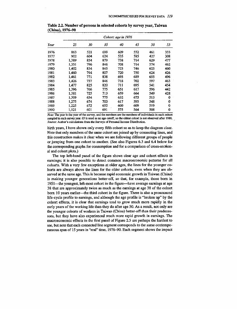
ECONOMETRIC ISSUES FOR SURVEY DATA 119
Table 2.2. Number of persons in selected cohorts by survey year, Taiwan(China), 1976-90
Cohort: age in 1976
Year 25 30 35 40 45 50 55
1976 863 521 699 609 552 461 3331977 902 604 624 535 585 427 3081978 1,389 854 879 738 714 629 4771979 1,351 796 846 708 714 574 4621980 1,402 834 845 723 746 625 4601981 1,460 794 807 720 750 624 4261982 1,461 771 838 695 689 655 4961983 1,426 737 846 718 702 597 4631984 1,477 825 820 711 695 541 4541985 1,396 766 775 651 617 596 4421986 1,381 725 713 659 664 549 4281987 1,309 634 775 632 675 513 01988 1,275 674 700 617 595 548 01989 1,225 672 652 600 609 519 01990 1,121 601 691 575 564 508 0Note: The year is the year of the survey, and the numbers are the numbers of individuals in each cohortsampled in each survey year. 65 is used as an age cutoff, so the oldest cohort is not observed after 1986.Source: Author's calculations from the Surveys of Personal Income Distribution.
birth years, I have shown only every fifth cohort so as to keep the diagram clear.Note that only members of the same cohort are joined up by connecting lines, andthis construction makes it clear when we are following different groups of peopleor jumping from one cohort to another. (See also Figures 6.3 and 6.4 below forthe corresponding graphs for consumption and for a comparison of cross-section-al and cohort plots.)
The top left-hand panel of the figure shows clear age and cohort effects inearnings; it is also possible to detect common macroeconomic patterns for allcohorts. With a very few exceptions at older ages, the lines for the younger co-horts are always above the lines for the older cohorts, even when they are ob-served at the same age. This is because rapid economic growth in Taiwan (China)is making younger generations better-off, so that, for example, those born in1951-the youngest, left-most cohort in the figure-have average earnings at age38 that are approximately twice as much as the earnings at age 38 of the cohortborn 10 years earlier-the third cohort in the figure. There is also a pronouncedlife-cycle profile to earnings, and although the age profile is "broken up" by thecohort effects, it is clear that earnings tend to grow much more rapidly in theearly years of the working life than they do after age 50. As a result, not only arethe younger cohorts of workers in Taiwan (China) better-off than their predeces-sors, but they have also experienced much more rapid growth in earnings. Themacroeconomic effects in the first panel of Figure 2.5 are perhaps the hardest tosee, but note that each connected line segment corresponds to the same contempo-raneous span of 15 years in "real" time, 1976-90. Each segment shows the impact

120 THE ANALYSIS OF HOUSEHOLD SURVEYS
of the slowdown in Taiwanese economic growth after the 1979 oil shock. Eachcohort has very rapid growth from the second to third year observed, which is1977-78, somewhat slower growth for the next two years, 1978-80, and then twoyears of slow or negative growth after the shock. This decomposition into cohort,age, and year effects can be formalized in a way that will work even when thedata are not annual and not necessarily evenly spaced, a topic to which I return inthe final subsection below. Before that, however, it is useful to use this exampleto highlight the advantages and disadvantages of cohort data more generally.
Cohort data versus panel data
A useful comparison is between the semiaggregated cohort data and genuinepanel data in which individual households are tracked over time. In both cases,we have a time series of observations on a number of units, with units defined aseither cohorts or individuals. The cohort data cannot tell us anything about dy-namics within the cohorts; each survey tells us about the distribution of the char-acteristic in the cohort in each period, but two adjacent surveys tell us nothingabout the joint distribution of the characteristic in the two periods. In the earningsexample, the time series of cross sections can tell us about average earnings forthe cohort over time, and it can tell us about inequality of earnings within thecohort and how it is changing over time, but it cannot tell us how long individualsare poor, or whether the people ftho are rich now were rich or poor at some ear-lier date. But apart from dynamics, the cohort data can do most of what would beexpected of panel data. In particular, and as we shall see in the next subsection,the cohort data can be used to control for unobservable fixed effects just as withpanel data, a feature that is often thought to be the main econometric attraction ofthe latter.
Cohort data also have a number of advantages over most panels. As we haveseen in Chapter 1, many panels suffer from attrition, especially in the early years,and so run the risk of becoming increasingly unrepresentative over time. Becausethe cohort data are constructed from fresh samples every year, there is no attri-tion. There will be (related) problems with the cohort data if the sampling designchanges over time, or if the probabilities of selection into the sample depend onage as, for example, for young men undergoing military training. The way inwhich the cohort data are used will often be less susceptible to measurement errorthan is the case with panels. The quantity that is being tracked over time is typi-cally an average (or some other statistic such as the median or other percentile)and the averaging will nearly always reduce the effects of measurement error andenhance the signal-to-noise ratio. In this sense, cohort methods can be regarded asiv methods, where the instruments are grouping variables, whose applicationaverages away the measurement error. Working with aggregated data at a levelthat is intermediate between micro and macro also brings out the relationshipbetween household behavior and the national aggregates and helps bridge the gapbetween them; in Figure 2.5, for example, the behavior of the aggregate economyis clearly apparent in the averages of the household data.

ECONOMETRIC ISSUES FOR SURVEY DATA 121
It should be emphasized that cohort data can be constructed for any character-istic of the distribution of interest; we are not confined to means. As we shall seein Chapter 6, it can be interesting and useful to study how inequality changeswithin cohorts over time, and since we have the micro data for each cohort ineach year, it is as straightforward to work with measures of dispersion as it is towork with measures of central tendency. Medians can be used instead of means-a technique that is often useful in the presence of outliers-and if the theory sug-gests working with some transform of the data, the transform can be made prior toaveraging. When working with aggregate data, theoretical considerations oftensuggest working with the mean of a logarithm, for example, rather than with thelogarithm of the mean. The former is not available from aggregate data, but canbe routinely computed from the micro data when calculating the semiaggregatedcohort averages.
A final advantage of cohort methods is that they allow the combination of datafrom different surveys on different households. The means of cohort consumptionfrom an expenditure survey can be combined with the means of cohort incomefrom a labor force survey, and the hybrid data set used to study saving. It is notnecessary that all variables are collected from the same households in one survey.
Against the use of cohort data, it should be noted that there are sometimesproblems with the assumption that the cohort population is constant, an assump-tion that is needed if the successive surveys are to generate random samples fromthe same underlying population. I have already noted potential problems withmilitary service, migration, aging, and death. But the more serious difficultiescome when we are forced to work, not with individuals, but with households, andto define cohorts of households by the age of the head. If households once formedare indissoluble, there would be no difficulty, but divorce and remarriage reorga-nize households, as does the process whereby older people go to live with theirchildren, so that previously "old" households become "young" households in sub-sequent years. It is usually clear when these problems are serious, and they affectsome segments of the population more than others, so that we know which data totrust and which to suspect.
Panel data from successive cross sections
It is useful to consider briefly the issues that arise when using cohort data as ifthey were repeated observations on individual units. I show first how fixed effectsat the individual level carry through to the cohort data, and what steps have to betaken if they are to be eliminated. Consider the simplest univariate model withfixed effects, so that at the level of the individual household, we have (2.76) witha single variable
(2.84) Yit = a +.pxi,+Pt,Oi+ui,
where the ,u are year dummies and O6 is an individual-specific fixed effect. Ifthere were no fixed effects, it would be possible to average (2.84) over all the

122 THE ANALYSIS OF HOUSEHOLD SURVEYS
households in each cohort in each year to give a corresponding equation for thecohort averages. When there are fixed effects, (2.84) still holds for the cohortpopulation means, with cohort fixed effects replacing the individual fixed effects.However, if we average (2.84) over the members of the cohorts who appear in thesurvey, and who will be different from year to year, the "fixed effect" will not befixed, because it is the average of the fixed effects of different households in eachyear. Because of this sampling effect, we cannot remove the cohort fixed effectsby differencing or using within-estimators.
Consider an alternative approach based on the unobservable population meansfor each cohort. Start from the cohort version of (2.84), and denote populationmeans in cohorts by the subscripts c, so that, simply changing the subscript i to c,we have
(2.85) Yc, = a+IpxC+P +Oc+u,
and take first differences-the comparable analysis for the within-estimator is leftas an exercise-to eliminate the fixed effects so that
(2.86) Ayc, = Ap, + PAxC, + Au,
where the first term is a constant in any given year. This procedure has eliminatedthe fixed effects, but we are left with the unobservable changes in the populationcohort means in place of the sample cohort means, which is what we observe. Ifwe replace Ay and Ax in (2.84) by the observed changes in the sample means,we generate an error-in-variables problem, and the estimates will be attenuated.
There are at least two ways of dealing with this problem. The first is to notethat, just as the sample was used to provide an estimate of the cohort mean, it canalso be used to provide an estimate of the standard error of the estimate, which inthis context is the variance of the measurement error. For the example (2.86), wecan use overbars to denote sample means and write
(2.87) AsY, = Ay,, + E2, -El,ct-,( . ) ~~~~~A XCt = A xCt + E2,t -'E2,t-I
where Etc, and e&, are sampling errors in the cohort means. Because they comefrom different surveys with independently selected samples, they are independent
2 2over time, and their variances and covariance, a,, a2, and 0,2 are calculated inthe usual way, from the variances and covariance in the sample divided by thecohort size (with correction for cluster effects as necessary.) From (2.87), we seethat the variances and covariances of the sample cohort means are inflated by thevariances and covariances of the sampling errors, but that, if these are subtractedout, we can obtain consistent estimates of P in (2.86) from-cf. also (2.62) above,
cov(AX.8Ay8-) - 012, - G12t-1
var(A5%,) - a2 - <2
and where, for illustrative purposes, I have assumed that there are only two timeperiods t and t - 1. The standard error for (2.88) can be calculated using the boot-strap or the delta method-discussed in the next section-which can also take

ECONOMETRIC ISSUES FOR SURVEY DATA 123
into account the fact that the variance and covariances of the sampling errors areestimated (see Deaton 1985, who also discusses the multivariate case, and Fuller1987, who gives a general treatment for a range of similar models).
Another possible estimation strategy is to use IV, with changes from earlieryears used as instruments. Since the successive samples are independently drawn,changes in cohort means from t -2 to t - 1 are measured independently of thechange from t to t + 1. In some cases, the cohort samples may be large enoughand the means precisely enough estimated so that these corrections are smallenough to ignore. In any case, it is a good idea to check the standard errors of thecohort means, to make sure that regression results are not being dominated bysampling effects, and if so, to increase the cohort sizes, for example, by workingwith five-year age bands instead of single years. In some applications, this mightbe desirable on other grounds; in some countries, people do not know their datesof birth well enough to be able to report age accurately, and reported ages "heap"at numbers ending in 5 and 0.
Decompositions by age, cohort, and year
A number of the quantities most closely associated with welfare, including familysize, earnings, income, and consumption, have distinct and characteristic life-cycle profiles. Wage rates, earnings, and saving usually have hump-shaped ageprofiles, rising to their maximum in the middle years of life, and declining some-what thereafter. The natural process of bearing and raising children induces asimilar profile in average family size. Moreover, all of these quantities are subjectto secular variation; consumption, earnings, and incomes rise over time witheconomic development, and family size decreases as countries pass through thedemographic transition. In consequence, even if the shape of the age profiles re-mains the same for successive generations, their position will shift from one to thenext. The age profile from a single cross section confounds the age profile withthe generational or cohort effects. For example, a cross-sectional earnings profilewill tend to exaggerate the downturn in earnings at the highest age because, as welook at older and older individuals, we are not just moving along a given age-earnings profile, but we are also moving to ever lower lifetime profiles. The co-hort data described in this section allow us to track the same cohort over severalyears and thus to avoid the difficulty; indeed, the Taiwanese earnings example inFigure 2.5 provides a clear example of the differences between the age profiles ofdifferent cohorts. In many cases, diagrams like Figure 2.5 will tell us all that weneed to know. However, since each cohort is only observed for a limited period oftime, it is useful to have a technique for linking together the age profiles fromdifferent cohorts to generate a single complete life-cycle age profile. This is par-ticularly true when there is only a limited number of surveys, and the intervalsbetween them are more than one year. In such cases, diagrams like Figure 2.5 areharder to draw, and a good deal less informative.
In this subsection, I discuss how the cohort data can be decomposed into ageeffects, cohort effects, and year effects, the first to give the typical age profile, the

124 THE ANALYSIS OF HOUSEHOLD SURVEYS
second the secular trends that lead to differences in the positions of age profilesfor different cohorts, and the third the aggregate effects that synchronously buttemporarily move all cohorts off their profiles. These decompositions are basedon models and are certainly not free of structural assumptions; they assume awayinteraction effects between age, cohort, and years, so that, for example, the shapeof age profiles is unaffected by changes in their position, and the appropriatenessand usefulness of the assumption has to be judged on a case-by-case basis.
To make the analysis concrete, consider the case of the lifetime consumptionprofile. If the growth in living standards acts so as to move up the consumption-age profiles proportionately, it makes sense to work in logarithms, and to writethe logarithm of consumption as
(2.89) Incc, = ,+ a + Yc + *t + uCZ
where the superscripts c and t (as usual) refer to cohort and time (year), and arefers to age, defined here as the age of cohort c in year t. In this particular case,(2.89) can be given a theoretical interpretation, since according to life-cycle the-ory under certainty, consumption is the product of lifetime wealth, the cohortaggregate of which is constant over time, and an age effect, which is determinedby preferences (see Section 6.1 below). In other contexts where there is no suchtheory, the decomposition is often a useful descriptive device, as for earnings inTaiwan (China), where it is hard to look at the top left-hand panel of Figure 2.5without thinking about an age and cohort decomposition.
In order to implement a model like (2.89), we need to decide how to labelcohorts. A convenient way to do so is to choose c as the age in year t =0. By this,c is just a number like a and t. We can then choose to restrict the age, cohort, andyear effects in (2.89) in various different ways. In particular, we can choose poly-nomials or dummies. For the year effects, where there is no obvious pattern apriori, dummy variables would seem to be necessary, but age effects could rea-sonably be modeled as a cubic, quartic, or quintic polynomial in age, and cohorteffects, which are likely to be trend-like, might even be adequately handled aslinear in c. Given the way in which we have defined cohorts, with bigger valuesof c corresponding to older cohorts, we would expect yc to be declining with c.When data are plentiful, as in the Taiwanese case, there is no reason not to usedummy variables for all three sets of effects, and thus to allow the data to chooseany pattern.
Suppose that A is a matrix of age dummies, C a matrix of cohort dummies, andY a matrix of year dummies. The cohort data are arranged as cohort-year pairs,with each "observation" corresponding to a single cohort in a specific year. Ifthere are m such cohort-year pairs, the three matrices will each have m rows; thenumber of columns will be the number of ages (or age groups), the number ofcohorts, and the number of years, respectively. The model (2.89) can then bewritten in the form
(2.90) y = +Aa+Cy+Yd,i+u

ECONOMETRIC ISSUES FOR SURVEY DATA 125
where y is the stacked vector of cohort-year observations-each row correspondsto a single observation on a cohort-on the cohort means of the logarithm of con-sumption. As usual, we must drop one column from each of the three matrices,since for the full matrices, the sum of the columns is a column of ones, which isalready included as the constant term.
However, even having dropped these columns, it is still impossible to estimate(2.90) because there is an additional linear relationship across the three matrices.The problem lies in the fact that if we know the date, and we know when a cohortwas born, then we can infer the cohort's age. Indeed, since c is the age of thecohort in year 0, we have
(2.91) act = c + t
which implies that the matrices of dummies satisfy
(2.92) Asa = Csc + Ysy
where the s vectors are arithmetic sequences { 0,1,2,3, . . of the length givenby the number of columns of the matrix that premultiplies them. Equation (2.92)is a single identity, so that to estimate the model it is necessary to drop one morecolumn from any one of the three matrices.
The normalization of age, cohort, and year effects has been discussed in dif-ferent contexts by a number of authors, particularly Hall (1971), who provides anadmirably clear account in the context of embodied and disembodied technicalprogress for different vintages of pickup trucks, and by Weiss and Lillard (1978),who are concerned with age, vintage, and time effects in the earnings of scientists.The treatment here is similar to Hall's, but is based on that given in Deaton andPaxson (1994a). Note first that in (2.90), we can replace the parameter vectors a,y, and * by
(2.93) = a +Ksa, ' =y -KSc, vsy = -KSy
for any scalar constant Kc, and by (2.92) there will be no change in the predictedvalue of y in (2.87). According to (2.90), a time-trend can be added to the agedummies, and the effects offset by subtracting time-trends from the cohort dum-mies and the year dummies.
Since these transformations are a little hard to visualize, and a good deal morecomplicated than more familiar dummy-variable normalizations, it is worth con-sidering examples. Suppose first that consumption is constant over cohorts, ages,and years, so that the curves in Figure 2.5 degenerate to a single straight line withslope 0. Then we could "decompose" this into a positive age effect, with con-sumption growing at (say) five percent for each year of age, and offset this by anegative year effect of five percent a year. According to this, each cohort wouldget a five percent age bonus each year, but would lose it to a macroeconomiceffect whereby everyone gets five percent less than in the previous year. If this

126 THEANALYSISOFHOUSEHOLDSURVEYS
were all, younger cohorts would get less than older cohorts at the same age, be-cause they come along later in time. To offset this, we need to give each cohortfive percent more than the cohort born the year previously which, since the oldercohorts have higher cohort numbers, means a negative trend in the cohort effects.More realistically, suppose that when we draw Figure 2.5, we find that the con-sumption of each cohort is growing at three percent a year, and that each succes-sive cohort's profile is three percent higher than that of its predecessor. Everyonegets three percent more a year as they age, and starting consumption rises by threepercent a year. This situation can be represented (exactly) by age effects that riselinearly with age added to cohort effects that fall linearly with age by the sameamount each year; note that cohorts are labeled by age at a fixed date, so thatolder cohorts (larger c) are poorer, not richer. But the same data can be represent-ed by a time-trend of three percent a year in the age effects, without either cohortor year effects.
In practice, we choose a normalization that is most suitable for the problem athand, attributing time-trends to year effects, or to matching age and cohort ef-fects. In the example here, where consumption or earnings is the variable to bedecomposed, a simple method of presentation is to attribute growth to age andcohort effects, and to use the year effects to capture cyclical fluctuations or busi-ness-cycle effects that average to zero over the long run. A normalization thataccomplishes this makes the year effects orthogonal to a time-trend, so that, usingthe same notation as above,
(2.94) s,y = 0.
The simplest way to estimate (2.90) subject to the normalization (2.94) is to re-gress y on (a) dummies for each cohort excluding (say) the first, (b) dummies foreach age excluding the first, and (c) a set of T- 2 year dummies defined as fol-lows, from t = 3,.., T
(2.95) d, = d,-[(t-1)d 2 -(t-2)d 11
where dt is the usual year dummy, equal to 1 if the year is t and 0 otherwise. Thisprocedure enforces the restriction (2.94) as well as the restriction that the yeardummies add to zero. The coefficients of the di* give the third through final yearcoefficients; the first and second can be recovered from the fact that all year ef-fects add to zero and satisfy (2.94).
This procedure is dangerous when there are few surveys, where it is difficultto separate trends from transitory shocks. In the extreme case where there are onlytwo years, the method would attribute any increase in consumption between thefirst and second years to an increasing age profile combined with growth fromolder to younger cohorts. Only when there are sufficient years for trend and cycleto be separated can we make the decomposition with any confidence.
The three remaining panels of Figure 2.5 show the decomposition of the earn-ings averages into age, cohort, and year dummies. The cohort effects in the top

ECONOMETRIC ISSUES FOR SURVEY DATA 127
right-hand panel are declining with age; the earlier you are born, the older you arein 1976, and age in 1976 is the cohort measure. Although the picture is one that isclose to steady growth from cohort to cohort, there has been a perceptibleacceleration in the rate of growth for the younger cohorts. The bottom left-handpanel shows the estimated age effects; according to this, wages are a concavefunction of age, and although there is little wage increase after age 50, there is noclear turning down of the profile. Although the top left panel creates an impres-sion of a hump-shaped age profile of earnings, much of the impression comesfrom the cohort effects, not the age effects, and although the oldest cohort shownhas declining wages from ages 58 through 65, other cohorts observed at the sameages do not display the same pattern. (Note that only every fifth cohort is includedin the top left panel, but all cohorts are included in the regressions, subject only toage lying being between 25 and 65 inclusive.) The final panel shows the yeareffects, which are estimated to be much smaller in magnitude than either thecohort or age effects; nevertheless they show a distinctive pattern, with the econ-omy growing much faster than trend at the beginning and end of the period, andmuch more slowly in the middle after the 1979 oil shock.
Age and cohort profiles such as those in Figure 2.5 provide the material forexamining the structural consequences of changes in the rates of growth of popu-lation and real income. For example, if the age profiles of consumption and in-come are determined by tastes and technology, and are invariant to changes in therate of economic growth, we can change the cohort effects holding the age effectsconstant and thus derive the effects of growth on aggregates of consumption,saving, and income. Changes in population growth rates redistribute the popula-tion over the various ages, so that, once again, we can use the age profiles as thebasis for aggregating over different age distributions of the population. Much pre-vious work has been forced to rely on single cross sections to estimate age pro-files, and while this is sometimes the best that can be done, cross-sectional ageprofiles confuse the cohort and age effects, and will typically give much less reli-able estimates than the methods discussed in this section. I return to these tech-niques in the final chapter when I come to examine household saving behavior.
2.8 Two issues in statistical inference
This final section deals briefly with two topics that will be required at variouspoints in the rest of the book, but which do not fit easily into the rest of this chap-ter. The first deals with a situation that often arises in practice, when the parame-ters of interest are not the parameters that are estimated, but functions of them. Ibriefly explain the "delta" method which allows us to transform the variance-covariance matrix of the estimated parameters into the variance-covariance matrixof the parameters of interest, so that we can construct hypothesis tests for thelatter. Even when we want to use the bootstrap to generate confidence intervals,asymptotic approximation to variances are useful starting points that can be im-proved using the bootstrap (see Section 1.4). The second topic is concerned withsample size, and its effects on statistical inference. Applied econometricians often

128 THE ANALYSIS OF HOUSEHOLD SURVEYS
express the view that rejecting a hypothesis using 100 observations does not havethe same meaning as rejecting a hypothesis using 10,000 observations, and thatnull hypotheses are more often rejected the larger is the sample size. Householdsurveys vary in size from a few hundred to tens or even hundreds of thousands ofobservations, so that if inference is indeed the hostage of sample size, it is import-ant to be aware of exactly what is going on, and how to deal with it in practice.
*Parameter transformations: the delta method
Suppose that we have estimates of a parameter vector ,, but that the parametersof interest are not P, but some possibly nonlinear transformation a, where
(2.96) a = h(p)
for some known vector of differentiable functions h. In general, this function willalso depend on the data, or on some characteristics of the data such as samplemeans. It will also usually be the case that a and P will have different numbers ofelements, k for , and q for a, with q • k. Our estimation method has yielded anestimate , for , and an associated variance-covariance matrix V, for which anestimate is also available. The delta method is a means of transforming V, intoV.; a good formal account is contained in Fuller (1987, pp. 85-88). Here I con-fine myself to a simple intuitive outline.
Start by substituting the estimate of ,B to obtain the obvious estimate of a,a = h (n). If we then take a Taylor series approximation of a = h ( ) around thetrue value of ,B, we have for i = 1 ... q,
kah(2.97) di & ai + E3 pi)
or in an obvious matrix notation
(2.98) & H(O - ).
The matrix H is the qxk Jacobian matrix of the transformation. If we then post-multiply (2.98) by its transpose and take expectations, we have
(2.99) Va HVpHW.
In practice (2.99) is evaluated by replacing the three terms on the right-hand sideby their estimates calculated from the estimated parameters. The estimate of thematrix H can either be programmed directly once the differentiation has beendone analytically, or the computer can be left to do it, either using the analyticaldifferentiation software that is increasingly incorporated into some econometricpackages, or by numerical differentiation around the estimates of P.
Variance-covariance matrices from the delta method are often employed tocalculate Wald test statistics for hypotheses that place nonlinear restrictions on the

ECONOMETRIC ISSUES FOR SURVEY DATA 129
parameters. The procedure follows immediately from the analysis above by writ-ing the null hypothesis in the form:
(2.100) Ho a = h(,) = 0
for which we can compute the Wald statistic
(2.101) W = &,val.-.
Under the null hypothesis, W is asymptotically distributed as X2 with q degrees offreedom. For this to work, the matrix Va has to be nonsingular, for which anecessary condition is that q be no larger than k; clearly we must not try to test thesame restriction more than once.
As usual, some warnings are in order. These results are valid only as large-sample approximations, and may be seriously misleading in finite samples. Forexample, the ratio of two normally distributed variables has a Cauchy distributionwhich does not possess any moments, yet the delta method will routinely providea "variance" for this case. In the context of the Wald tests of nonlinear restric-tions, there are typically many different ways of writing the restrictions, and un-less the sample size is large and the hypothesis correct, these will all lead to dif-ferent values of the Wald test (see Gregory and Veall 1985 and Davidson andMacKinnon 1993, pp. 463-7 1, for further discussion).
Sample size and hypothesis tests
Consider the frequently encountered situation where we wish to test a simple nullhypothesis against a compound alternative, that j3 = Po for some known poagainst the alternative ,B 9# Po. A typical method for conducting such a test wouldbe to calculate some statistic from the data and to see how far it is from the valuethat it would assume under the null, with the size of the discrepancy acting asevidence against the null hypothesis. Most obviously, we might estimate f3 itselfwithout imposing the restriction, and compare its value with Po Likelihood-ratiotests-or other measures based on fit-compare how well the model fits the dataat unrestricted and restricted estimates of P. Score-or Lagrange multiplier-testscalculate the derivative of the criterion function at Po, on the grounds that non-zero values indicate that there are better-fitting alternatives nearby, so castingdoubt on the null. All of these supply a measure of the failure of the null, and ouracceptance and rejection of the hypothesis can be based on how big is the mea-sure.
The real differences between different methods of hypothesis testing come,not in the selection of the measure, but in the setting of a critical value, abovewhich we reject the hypothesis on the grounds that there is too much evidenceagainst it, and below which we accept it, on the grounds that the evidence is notstrong enough to reject. Classical statistical procedures-which dominate econo-metric practice-set the critical value in such a way that the probability of reject-

130 THE ANALYSIS OF HOUSEHOLD SURVEYS
ing the null when it is correct, the probability of Type I error, or the size of thetest, is fixed at some preassigned level, for example, five or one percent. In theideal situation, it is possible under the null hypothesis to derive the samplingdistribution of the quantity that is being used as evidence against the null, so thatcritical values can be calculated that will lead to exactly five (one) percent ofrejections when the null is true. Even when this cannot be done, the asymptoticdistribution of the test statistic can usually be derived, and if this is used to selectcritical values, the null will be rejected five percent of the time when the samplesize is sufficiently large. These procedures take no explicit account of the powerof the test, the probability that the null hypothesis will be rejected when it is false,or its complement, the Type II error, the probability of not rejecting the null whenit is false. Indeed, it is hard to see how these errors can be controlled because thepower depends on the unknown true values of the parameter, and tests will typi-cally be more powerful the further is the truth from the null.
That classical procedures can generate uncomfortable results as the samplesize increases is something that is often expressed informally by practitioners, andthe phenomenon has been given an excellent treatment by Leamer (1978, pp.100- 120), and it is on his discussion that the following is based.
The effect most noted by empirical researchers is that the null hypothesisseems to be more frequently rejected in large samples than in small. Since it ishard to believe that the truth depends on the sample size, something else must begoing on. If the critical values are exact, and if the null hypothesis is exactly true,then by construction the null hypothesis will be rejected the same fraction oftimes in all sample sizes; there is nothing wrong with the logic of the classicaltests. But consider what happens when the null is not exactly true, or alterna-tively, that what we mean when we say that the null is true is that the parametersare "close" to the null, "close" referring to some economic or substantive mean-ing that is not formally incorporated into the statistical procedure. As the samplesize increases, and provided we are using a consistent estimation procedure, ourestimates will be closer and closer to the truth, and less dispersed around it, sothat discrepancies that were undetectable with small sample sizes will lead torejections in large samples. Larger sample sizes are like greater resolving poweron a telescope; features that are not visible from a distance become more andmore sharply delineated as the magnification is turned up.
Over-rejection in large samples can also be thought about in terms of Type Iand Type II errors. When we hold Type I error fixed and increase the sample size,all the benefits of increased precision are implicitly devoted to the reduction ofType II error. If there are equal probabilities of rejecting the null when it is trueand not rejecting it when it is false at a sample size of 100, say, then at 10,000, wewill have essentially no chance of accepting it when it is false, even though weare still rejecting it five percent of the time when it is true. For economists, whoare used to making tradeoffs and allocating resources efficiently, this is a verystrange thing to do. As Leamer points out, the standard defense of the fixed sizefor classical tests is to protect the null, controlling the probability of rejecting itwhen it is true. But such a defense is clearly inconsistent with a procedure that
ECONOMETRIC ISSUES FOR SURVEY DATA 131
devotes none of the benefit of increased sample size to lowering the probabilitythat it will be so rejected.
Repairing these difficulties requires that the critical values of test statistics beraised with the sample size, so that the benefits of increased precision are moreequally allocated between reduction in Type I and Type II errors. That said, it is agood deal more difficult to decide exactly how to do so, and to derive the rulefrom basic principles. Since classical procedures cannot provide such a basis,Bayesian alternatives are the obvious place to look. Bayesian hypothesis testing isbased on the comparison of posterior probabilities, and so does not suffer fromthe fundamental asymmetry between null and alternative that is the source of thedifficulty in classical tests. Nevertheless, there are difficulties with the Bayesianmethods too, perhaps most seriously the fact that the ratio of posterior probabili-ties of two hypotheses is affected by their prior probabilities, no matter what thesample size. Nevertheless, the Bayesian approach has produced a number of pro-cedures that seem attractive in practice, several of which are reviewed by Leamer.
It is beyond the scope of this section to discuss the Bayesian testing proce-dures in any detail. However, one of Leamer's suggestions, independently pro-posed by Schwarz (1978) in a slightly different form, and whose derivation is alsoinsightfully discussed by Chow (1983, pp. 300-2), is to adjust the critical valuesfor F and x2 tests. Instead of using the standard tabulated values, the null is re-jected when the calculated F-value exceeds the logarithm of the sample size, Inn,or when a X2 statistic for q restrictions exceeds qlnn. To illustrate, when thesample size is 100, the null hypothesis would be rejected only if calculated F-statistics are larger than 4.6, a value that would be doubled to 9.2 when workingwith sample sizes of 10,000.
In my own work, some of which is discussed in the subsequent chapters of thisbook, I have often found these Leamer-Schwarz critical values to be useful. Thisis especially true in those cases where the theory applies most closely, when weare trying to choose between a restricted and unrestricted model, and when wehave no particular predisposition either way except perhaps simplicity, and wewant to know whether it is safe to work with the simpler restricted model. If theLeamer- Schwarz criterion is too large, experience suggests that such simplifica-tions are indeed dangerous, something that is not true for classical tests, wherelarge-sample rejections can often be ignored with impunity.
2.9 Guide to further reading
The aim of this chapter has been to extract from the recent theoretical and appliedeconometric literature material that is useful for the analysis of household-leveldata. The source of the material was referenced as it was introduced, and in mostcases, there is little to consult apart from these original papers. I have assumedthat the reader has a good working knowledge of econometrics at the level of anadvanced undergraduate, masters', or first-year graduate course in econometricscovering material such as that presented in Pindyck and Rubinfeld (1991). At thesame level, the text by Johnston and DiNardo (1996) is also an excellent starting

132 THE ANALYSIS OF HOUSEHOLD SURVEYS
point and, on many topics, adopts an approach that is sympathetic to that takenhere. A more advanced text that covers a good deal of the modern theoreticalmaterial is Davidson and MacKinnon (1993), but like other texts it is not writtenfrom an applied perspective. Cramer (1969), although now dated, is one of thefew genuine applied econometrics texts, and contains a great deal that is stillworth reading, much of it concerned with the analysis of survey data. Some of thematerial on clustering is discussed in Chapter 2 of Skinner, Holt, and Smith(1989). Groves (1989, ch. 6) contains an excellent discussion of weighting in thecontext of modeling versus description. The STATA manuals, Stata Corporation(1993), are in many cases well ahead of the textbooks, and provide brief discus-sions and references on each of the topics with which they deal.
Related Documents