Spatially Balanced Sampling Methods in Household Surveys A thesis submitted in partial fulfilment of the requirements for the degree of Doctor of Philosophy in Statistics By Naeimeh Abi Supervised by Prof. Jennifer Brown Assoc. Prof. Elena Moltchanova Dr. Blair Robertson Mr. Richard Penny School of Mathematics and Statistics University of Canterbury May, 2019

Welcome message from author
This document is posted to help you gain knowledge. Please leave a comment to let me know what you think about it! Share it to your friends and learn new things together.
Transcript
Spatially Balanced Sampling Methods in Household
Surveys
A thesis submitted in partial fulfilment of the requirements for the degree of
Doctor of Philosophy in Statistics
By
Naeimeh Abi
Supervised by
Prof. Jennifer Brown
Assoc. Prof. Elena Moltchanova
Dr. Blair Robertson
Mr. Richard Penny
School of Mathematics and Statistics
University of Canterbury
May, 2019
i
Abstract
Household surveys are the most common type of survey used for providing information
about the social and economic characteristics of a population of people. In these
surveys, information is usually collected by sampling the houses where people live and
then enumerating one or more persons at each home. Current sampling methodologies
used in designing household surveys generally do not take into account the spatial
structure of populations. This may lead to selection of units (i.e., households,
individuals) near to each other that usually provide similar information in the sample.
As a result, the selected sample tends to be less efficient than a sample that reflects all
attributes of the population.
Spatially balanced sampling is a popular design for selecting samples from
natural resources and environmental studies, which avoids selecting neighbouring units
in the same sample. Spatially balanced sampling design ensures the selection of a
representative sample by providing a spatial coverage of a region corresponding to the
population of interest.
This doctoral thesis aims to assess the possibility of applying spatially balanced
sampling in designing household surveys. After investigating spatially balanced
methods available in the literature, balanced acceptance sampling (BAS), developed by
Robertson et al (2013) is considered for further investigation in this study.
This research comprises two main parts: (1) exploring the characteristics of
BAS from a practical perspective, (2) promoting the application of spatially balanced
sampling in household surveys. The first part looks into the advantages of the BAS
method in practical cases. It aims to highlight the potential advantages of the BAS
method for selecting samples in practical situations in environmental studies. The
flexible characteristics of BAS and its practical benefits (e.g., being able to
accommodate missed sampling units and the ability to add extra sampling units during
survey implementation) discussed in the first part, show that BAS has the potential to
be extended for application in other surveys, specifically, household surveys.
In the second part, the applicability of spatially balanced sampling in household
surveys is assessed. A technique for selecting a spatially balanced sample from a
ii
discrete population, called BAS-Frame, is introduced. The spatial and statistical
properties of the proposed method are investigated through conducting simulation
studies using the census 2013 meshblocks of selected regions in New Zealand. The
results from these simulation studies show that the proposed method is sufficiently
robust in spreading the sample over the population of interest. In addition, it is seen
that applying spatially balanced sampling in selecting samples for household surveys
provides more precise estimates when compared to non-spatially balanced sampling
methods.
The feasibility of spatially balanced sampling methods to deal with some practical
aspects of designing a household survey is also investigated in the second part (e.g.,
designing a primary sampling unit (PSU) which meet a pre-specified minimum number
of sampling units, designing longitudinal surveys, and selecting a sample in the
presence of auxiliary variables). A method on the basis of the BAS-Frame is developed
to merge undersized units with their nearby units as much as possible to define PSUs.
A simulation study shows that the proposed method is more powerful than the
conventional method (i.e., the Kish method) in combining the undersized units with
their undersized neighbours. The application of the BAS-Frame for controlling overlap
between rotation groups in the longitudinal designs is discussed. Finally the
performance of the BAS-Frame in spreading the sample over the space of the auxiliary
variables available in the frame is investigated. This study shows that in the case of the
existence of a small number of auxiliary variables (fewer than five variables), the BAS-
Frame can provide a good spread, not only over the geographical space of the
population, but also over the space of the auxiliary variables.
This research, by studying multiple concepts of spatially balanced sampling, leads
to better understanding of these sampling methods, and the advantages of extending
their applications to household surveys

iii
Acknowledgements
I would like to express my profound gratitude to my supervisors, Professor
Jennifer Brown, Associate Professor Elena Moltchanova, Senior Lecturer Blair
Robertson and Mr. Richard Penny. Without their guidance, technical discussions,
continuous support and encouragement, this work would not have been possible.
I would also like to thank Stats NZ for providing me with official data used for
analysis in this dissertation.
Many thanks are due to my friends and colleagues for their support and friendship
which made these four years of my life memorable.
To my mother and father for their love, unwavering support, prayers and
understanding during my PhD studies. Finally, I am immensely appreciative of my
husband, Amir, for being the source of my joy, inspiration and encouragement.
iv
List of contents
Abstract .................................................................................................................... i
Acknowledgements ................................................................................................ iii
Introduction ........................................................................................... 1
1.1 Background ....................................................................................................... 1
1.2 Research Motivations........................................................................................ 2
1.3 Research Objectives and Scope of Work .......................................................... 4
1.4 Organization of Thesis ...................................................................................... 5
1.5 References ......................................................................................................... 7
Sampling Design Approaches ............................................................... 9
2.1 Introduction ....................................................................................................... 9
2.2 Essential Concepts and Notations ................................................................... 10
2.3 Probability Sampling Design .......................................................................... 11
2.4 Review on Some Classic Sampling Designs................................................... 12
2.4.1 Simple Random Sampling ....................................................................... 13
2.4.2 Stratified Sampling .................................................................................. 14
2.4.3 Cluster and Multistage Sampling ............................................................. 15
2.5 Sampling Designs in Household Surveys ....................................................... 16
2.5.1 Defining PSUs in Household Surveys ..................................................... 17
2.5.2 Stratifying PSUs in Household Surveys .................................................. 19
2.5.3 Sampling PSUs in Household Surveys .................................................... 19
2.5.4 Longitudinal Designs in Household Surveys ........................................... 19
2.6 Spatial Autocorrelation and Moran’s I Index ................................................. 20
2.6.1 Review of Some Spatially Balanced Sampling Methods ......................... 22
2.6.2 Parameter Estimation in Spatially Balanced Sampling Methods ............. 32
v
2.6.3 Spatial Coverage ...................................................................................... 33
2.7 Conclusions ..................................................................................................... 36
2.8 References ....................................................................................................... 36
Balanced Acceptance Sampling and its Application to an Intertidal
Survey .......................................................................................................................... 42
3.1 Introduction ..................................................................................................... 42
3.2 Background to BAS ........................................................................................ 42
3.2.1 Random Numbers and Methodology of BAS .......................................... 42
3.2.2 Selecting a Sample by BAS ..................................................................... 45
3.2.3 Inclusion Probabilities and Population Estimations ................................. 46
3.3 Application of BAS to a Semi-Realistic Dataset ............................................ 47
3.3.1 Population Description ............................................................................. 47
3.3.2 Sample Selection ...................................................................................... 49
3.3.3 Spatial Coverage and Parameter Estimation ............................................ 50
3.4 Further Discussions about BAS ...................................................................... 53
3.5 Conclusions ..................................................................................................... 55
3.6 References ....................................................................................................... 56
Population Characteristics and Performance of Balanced Acceptance
Sampling ...................................................................................................................... 57
4.1 Introduction ..................................................................................................... 57
4.2 Application of BAS on Populations With Different Spatial Autocorrelation . 58
4.2.1 Using BAS in Populations Where Observations Have a Gaussian
Distribution ............................................................................................................... 58
4.2.2 Using BAS in Populations Where Responses are Binary Data ................ 65
4.3 BAS for Stratified Populations ....................................................................... 72
4.3.1 Considering Same Sampling Fraction in Each Stratum ........................... 72
vi
4.3.2 Considering Different Sampling Fractions in Strata ................................ 77
4.4 Conclusions ..................................................................................................... 81
4.5 References ....................................................................................................... 82
Spatially Balanced Sampling Methods for Household Surveys ......... 83
5.1 Introduction ..................................................................................................... 83
5.2 Spatially Balanced Sampling Methods in Environmental Studies Versus
Household Surveys ....................................................................................................... 84
5.2.1 Suitability of Balanced Acceptance Sampling for Selecting Samples From
Discrete Populations.................................................................................................. 87
5.3 A Frame for BAS for Discrete Populations .................................................... 89
5.3.1 Spatial Properties of the BAS-Frame Technique ..................................... 95
5.3.2 Statistical Properties of the BAS-Frame Technique ................................ 98
5.3.3 Application of Spatially Balanced Sampling Methods on Real Data .... 104
5.4 Implementation of Spatially Balanced Sampling Methods on Stratified
Populations in Household Surveys .............................................................................. 109
5.4.1 BAS-Frame Technique for a Stratified Population ................................ 110
5.4.2 Spatially Balanced Sampling Methods When the Population is Stratified
Geographically ........................................................................................................ 112
5.4.3 Spatially Balanced Sampling When the Population is Stratified
Demographically ..................................................................................................... 115
5.5 Conclusions ................................................................................................... 123
5.6 References ..................................................................................................... 125
Properties of Sampling Frames for Spatial Sampling in Household
Surveys ...................................................................................................................... 127
6.1 Introduction ................................................................................................... 127
6.2 Spatially Balanced Sampling Methods in Conducting a Two-Stage Cluster
Sampling ..................................................................................................................... 128
vii
6.2.1 Stage 1 – Selecting Sample Area Units in the Presence of an Area
Frame ...................................................................................................................... 128
6.2.2 Stage 2 – Selecting Sample Households in the Presence of a List
Frame ...................................................................................................................... 133
6.3 Spatially Balanced Sampling Methods in the Presence of a List of Household
Registry ....................................................................................................................... 134
6.3.1 Cluster BAS-Frame Method .................................................................. 136
6.3.2 Application of the Cluster BAS-Frame Method .................................... 138
6.4 Application of Spatially Balanced Sampling Methods in Household Surveys
in Non-ideal Situations ................................................................................................ 141
6.4.1 Selecting a Spatially Balanced Sample From a Map Using the BAS
Method .................................................................................................................... 142
6.5 Conclusions ................................................................................................... 147
6.6 References ..................................................................................................... 148
Spatially Balanced Sampling Methods and Some Features of
Household Surveys .................................................................................................... 151
7.1 Introduction ................................................................................................... 151
7.2 Constructing PSUs in Household Surveys .................................................... 151
7.2.1 Using the BAS-Frame Technique for Combining Undersized
Neighbouring Units ................................................................................................. 154
7.2.2 Application of the Proposed Technique on the Christchurch
Meshblocks ............................................................................................................. 158
7.3 Spatially Balanced Sampling Methods and Longitudinal Designs ............... 160
7.3.1 Overlap Control between Different Household Surveys ....................... 166
7.4 Spatially Balanced Sampling Methods and Availability of Auxiliary
Information in the Design Stage ................................................................................. 168
7.4.1 The Principles of LPMs and BAS-Frame in Spreading the Samples Over
the Space of Auxiliary Variables ............................................................................ 168
viii
7.4.2 Efficiency of BAS-Frame and Number of Auxiliary Variables ............. 174
7.5 Conclusions ................................................................................................... 183
7.6 References ..................................................................................................... 184
Conclusions and Recommendations ................................................. 187
8.1 Key Contributions ......................................................................................... 188
8.1.1 Part 1: Practical Aspects of the BAS Method ........................................ 188
8.1.2 Part 2: Application of Spatially Balanced Sampling in Household
Surveys .................................................................................................................... 189
8.2 Recommendations for Future Work .............................................................. 195
8.3 References ..................................................................................................... 196
Appendix A An Algorithm for Simulating a Spatial Auto-Correlated Population
................................................................................................................................... 197
A.1 Introduction .................................................................................................. 197
A.2 Generating a Population With a Specified Spatial Auto-Correlation .......... 197
A.2.1 Generating a Spatially Auto-Correlated Bernoulli Population ............. 199
A.3 References .................................................................................................... 203
ix
List of Figures
Figure 2-1. Two grid patterns that are usually used in two-dimensional systematic
sampling: (a) a square lattice, (b) a triangular lattice. ................................................. 23
Figure 2-2 the first three levels of a hierarchical quadrat partitioning in GRTS
(courtesy of Stevens, D. and Olsen (2004))................................................................. 25
Figure 2-3 implementation of the Brewer and Hanif (2013) method for selecting
equal and unequal probability samples. ....................................................................... 26
Figure 2-4 An example of implementing the suboptimal LPM in a population with
15 units that have been ordered according to a relevant variable associated with the
distance. Solid squares denote decided units and white squares denote undecided units.
Unit 𝑖 = 7 is selected randomly. A local subset that contains unit 𝑖’s potential
neighbours is selected among undecided units by considering ℎ = 3. ....................... 30
Figure 2-5 The Voronoi polygons generated around sampling units in a given
population with 56 units. Selected sampling units are shown enlarged. ..................... 35
Figure 3-1 The arrangement of the first 10 Halton points with 𝑝1 = 2 and 𝑝2 = 3.
..................................................................................................................................... 44
Figure 3-2 Number of Nasima dotilliformis in the simulated population that covers
400×400 equal quadrats. .............................................................................................. 48
Figure 3-3 Moran scatter plot of number of crab burrows in the study area formed
by 400 × 400 quadrats. ............................................................................................... 49
Figure 3-4 A sample of size equal to 48 quadrats drawn using (a) the BAS method,
(b) the two-dimensional systematic sampling method, and (c) the simple random
sampling method, respectively. ................................................................................... 51
Figure 3-5 The 𝑉𝑎𝑟𝑐𝑜𝑚𝑝𝑙𝑒𝑥/𝑉𝑎𝑟𝑆𝑅𝑆 of two different sampling methods (BAS
and SYS) with different sample sizes. ......................................................................... 52
Figure 3-6 The resultant survey when only 30 quadrats instead of 48 quadrats are
selected with (a) BAS and (b) two-dimensional systematic sampling method,
respectively. ................................................................................................................. 53
x
Figure 3-7 Examples of sampling units selected using the two-dimensional
systematic sampling method from a study area with irregular shape: (a) the resultant
sample size = 5, (b) the resultant sample size =3. ....................................................... 55
Figure 4-1 The spatial features of the generated Gaussian population with different
Moran’s I indices. ........................................................................................................ 60
Figure 4-2 Trend of simulated variance of the HT estimator for Gaussian
populations amongst different levels of Moran’s I when BAS and SRS are used to select
different sample sizes (a) 𝑛 = 50, (b) 𝑛 = 100, ( c) 𝑛 = 150, (d) 𝑛 = 200, (e) 𝑛 =
250, (f) 𝑛 = 300 and (g) 𝑛 = 350. ............................................................................. 64
Figure 4-3 The ratio of variance of the HT estimator of the BAS method to the
variance of the HT estimator of SRS, 𝑟𝐵𝐴𝑆/𝑆𝑅𝑆, for Gaussian populations amongst
different levels of Moran’s I. ....................................................................................... 64
Figure 4-4 Spatial features of the generated population with a Bernoulli
distribution with parameter 𝑝 = 0.5. ........................................................................... 67
Figure 4-5 Trend of the estimated variance of the HT estimator for different levels
of Moran’s I in Bernoulli populations with 𝑝 = 0.5 when BAS and SRS are used to
select different sample sizes (a) 𝑛 = 50, (b) 𝑛 = 100, (c) 𝑛 = 150, (d) 𝑛 = 200, (e)
𝑛 = 250, (f) 𝑛 = 300 and (g) 𝑛 = 350. ..................................................................... 70
Figure 4-6 The ratio of the variance of the HT estimator of the BAS method to the
variance of the HT estimator of the SRS, 𝑟𝐵𝐴𝑆/𝑆𝑅𝑆, for populations with Bernoulli
distribution for different levels of Moran’s I. ............................................................. 71
Figure 4-7 Study area of the population of crabs, which is partitioned into four
different strata. ............................................................................................................. 73
Figure 4-8 Variance of the achieved HT estimator among 1000 simulated samples
selected by two different sampling designs (BAS with proportional allocation, and
BAS) for a range of sample sizes. ............................................................................... 77
Figure 4-9 Polygons (envelopes) of boundaries of samples selected by BAS with
stratified sampling and StratBAS along with average values of the calculated 𝐾𝑟 for a
xi
range of sample sizes (a) 𝑛 = 36, (b) 𝑛 = 81, (c) 𝑛 = 121, (d) 𝑛 = 169, (e) 𝑛 = 196,
(f) 𝑛 = 256, (g) 𝑛 = 289. ........................................................................................... 80
Figure 5-1 Google images of (a) a discrete population (www.hnzc.co.nz) and (b)
a continuous population (www.financialtribune.com). ............................................... 85
Figure 5-2 A spatial sample selected from a continuous population. .................. 86
Figure 5-3 Sampling areas selected by overlaying a grid on a small part of a city.
Selected areas are shown by . ................................................................................... 86
Figure 5-4 (a) An example of a discrete population (b) equal boxes are placed
around discrete units, (c) using the BAS method, a unit is selected if the Halton point
is within the unit’s box. The boxes of four selected sampling units are shown in red.
Solid triangles show Halton points are located outside the boxes. .............................. 88
Figure 5-5 An example of a discrete population in which sampling units are
located very close to each other. Very close units are shown in circles. Non-overlapping
boxes around these units are so small that using BAS would be inefficient. .............. 89
Figure 5-6 The geographical locations of 506 cases in Boston Housing Dataset.
The study area is divided vertically into two boxes (B1 and B2). Since the number of
units (houses) is even (506), it is not necessary to add an extra unit randomly to it. .. 90
Figure 5-7 Boxes created after the horizontal division. Horizontal division is done
in each box achieved in the previous step. In this example, each created box in the first
step contains 253 units, so an extra unit (red points) was added randomly to each box.
The current boxes are halved with the same count of units. ........................................ 91
Figure 5-8 Boston Housing data study area split into 64 boxes after the first six
levels of the partitioning process. During the partitioning process of the Boston
Housing data into 64 boxes with the same counts of units, some units are added
randomly; these units are shown in red. ...................................................................... 92
Figure 5-9 Units in the Boston Housing dataset that have the same longitude are
shown in red. Green points show units that have the same latitude. ........................... 93
xii
Figure 5-10 A regular frame based on the primary frame shown in Figure 5-8 for
selecting equal probability sampling units using the BAS method. This frame contains
64 equal-sized boxes that are addressed the same way as the primary frame. ............ 94
Figure 5-11 (a) Selected boxes using the BAS method from a regular frame, and
(b) the location of the selected boxes on the relevant primary frame. ......................... 95
Figure 5-12 An artificial population used in a spatial balance investigation of the
BAS-Frame technique, overlaid with a 10 × 10 grid of square cells. .......................... 96
Figure 5-13 Comparison of spatial balance of SRS, GRTS, BAS, LPM1 and SCPS
using the quadrat-based method. Results are based on using 1000 samples of size 50.
The achieved sample size is the number of samples that fell into each of the 100 square
cells. ............................................................................................................................. 96
Figure 5-14 A map of Christchurch meshblock boundaries including the centre of
each meshblock. .......................................................................................................... 98
Figure 5-15 Three different layers of Christchurch meshblocks showing their
densities. ...................................................................................................................... 99
Figure 5-16 Spatial trends of the response variable 𝑦 for all Christchurch
meshblocks and three different layers of the Christchurch meshblocks. .................. 101
Figure 5-17 A population consisting of 64 units which are stratified into two strata
(“x” and “o”). ............................................................................................................. 111
Figure 5-18 The first option for sample selection from a stratified population using
the BAS-Frame technique. ........................................................................................ 111
Figure 5-19 The second option for sample selection from a stratified population
using the BAS-Frame technique. ............................................................................... 112
Figure 5-20 Variance of 𝑚ℎ𝑖 among all iterations for all evaluated designs and all
sample sizes. .............................................................................................................. 119
Figure 5-21 Trends of ratio of variances related to each target variable among the
different sample sizes. ............................................................................................... 122
Figure 6-1 Achieved 𝜇(𝜁) for all evaluated methods and different sampling
fractions. .................................................................................................................... 131
xiii
Figure 6-2 Estimated 𝐷𝑒𝑓𝑓𝑐𝑜𝑚𝑝𝑙𝑒𝑥, 𝐶𝑃 for all evaluated methods and different
sampling fractions. .................................................................................................... 132
Figure 6-3 Two different rules of listing paths (Redrawn from Centers for Disease
Control (2010)). ......................................................................................................... 133
Figure 6-4 Locations of generated housing units in two meshblocks in
Christchurch. Red points show the locations of two-storey housing units. ............... 139
Figure 6-5 An example of an area frame shown on a map. In this map, the
boundaries of the area units (meshblocks) are clear. ................................................. 143
Figure 6-6 Illustration of a situation that centre of an irregular shaped area is not
located within the boundaries. ................................................................................... 143
Figure 6-7 A sample of size 10 meshblocks selected by (a) BAS and (b) SRS from
a map frame of a small part of Christchurch city. ..................................................... 145
Figure 6-8 Spatial distribution of area of some meshblocks considered in the
simulation study. ........................................................................................................ 146
Figure 7-1 The geographical position of units in the population described in
Example 7.1. .............................................................................................................. 155
Figure 7-2 (a) Vertical temporary boxes achieved after completing the first step of
the division, (b) total numbers of households in each created vertical temporary box.
................................................................................................................................... 156
Figure 7-3 (a) Horizontal temporary boxes which are achieved after completing
the second step of the division,(b) total numbers of households in each created
horizontal temporary box. ......................................................................................... 156
Figure 7-4 (a) Vertical temporary boxes achieved after completing the third step
of the division, (b) total numbers of households in each created vertical temporary box
in the third step. ......................................................................................................... 157
Figure 7-5 (a) Vertical permanent boxes achieved after completing the third step
of the division, (b) total numbers of households in each created vertical permanent box
in the third step. ......................................................................................................... 157
xiv
Figure 7-6 (a) final boxes after completing the division process, (b) total numbers
of households in each created box after completing the division process. ................ 158
Figure 7-7 (a) Average distances (𝑑) calculated using both methods for a range of
pre-specified PSU size thresholds varying from 2 to 60 households. (b) The total
distance to visit all the created PSUs. ........................................................................ 160
Figure 7-8 The ratio of 𝜁𝑛 for GRTS, BAS-Frame when compared to SRS and
each other for a situation when sampling units are added to the sample one by one over
a period of time. ......................................................................................................... 162
Figure 7-9 Sample dwellings allocated into 20 different rotation groups using the
BAS-Frame technique. Dwellings with same colour are in the same rotation group.
................................................................................................................................... 164
Figure 7-10 An example of a rotation pattern which is conducted quarterly for
three successive years. Rotation groups are defined by alphabetic characters. The
number of appearing of a rotation group in the sample is defined by its subscript: for
example 𝐾3 means that rotation group 𝐾 is revisited for the third time. Rotation groups
that are entered to the sample for the first time are shown in grey. ........................... 164
Figure 7-11 Spatial balance of the selected sampling units in each period. ...... 166
Figure 7-12 Sampling distribution of the auxiliary variables for three different
sampling methods among 1000 samples of size 10. .................................................. 172
Figure 7-13 Trend of average of spatial balance, 𝜁 , for each sampling method
amongst the number of auxiliary variables and for a range of sampling fractions: (a)
sampling fraction = 7%,( b) sampling fraction = 9% and (c) sampling fraction = 10%.
................................................................................................................................... 177
Figure 7-14 The “scree plot” for the PCs determined from the Christchurch
meshblocks dataset. ................................................................................................... 179
Figure 7-15 The simulated variances of the auxiliary variables for LPM and BAS-
Frame in relation to SRS for two situations: (1) when PC1 was the only auxiliary
variable in the sample selection process, and (2) when all 10 auxiliary variables were
considered in the sample selection process and for three sampling fractions: (a)

xv
sampling fraction = 7%,( b) sampling fraction = 9% and (c) sampling fraction = 10%.
................................................................................................................................... 182
xvi
List of Tables
Table 3-1 𝜇𝜁, the simulated variance of the HT estimator and the estimated
variance 𝑉𝑎𝑟𝑒𝑠𝑡 for two sampling schemes with different sample sizes. ................... 52
Table 4-1 Simulated variance of the HT estimator when BAS and SRS are
employed to select samples (of sizes 𝑛 = 50, 100, 150, 200, 250, 300 and 350) from
Gaussian populations with different levels of Moran’s I. ........................................... 61
Table 4-2 Simulated variance of the HT estimator for eight binary populations
with different levels of Moran’s I when 𝑝 = 0.5 and BAS and SRS are used to select
samples of size n=50, 100, 150, 200, 250, 300 and 350. ............................................. 68
Table 4-3 Average and variance of the observed quadrats in each stratum for 1000
samples selected by BAS and SRS for a range of different sample sizes. Sample sizes
allocated to each stratum if stratified sampling with proportional allocation were
applied, are shown in rows entitled “proportional”. .................................................... 75
Table 4-4 Simulated variance of the achieved HT estimator for 1000 simulated
samples and the average of the estimated variances for 1000 samples selected by two
different sampling designs (BAS with proportional allocation and BAS). ................. 76
Table 4-5 The average of 𝜁 for two sampling schemes (BAS with stratified
sampling and StratBAS) in different sample sizes. ..................................................... 78
Table 5-1 Comparison of the spatial balance of SRS, GRTS, BAS, LPM1 and
SCPS using the Voronoi polygons method. The values of 𝜇(𝜁)were estimated from
1000 simulated samples and for five different sample sizes. ...................................... 97
Table 5-2 Average area of meshblocks (𝑘𝑚2), density, and standard deviation
(𝑘𝑚2) of the area of Christchurch city meshblocks (𝑘𝑚2) in each layer................. 100
Table 5-3 The number of meshblocks and Moran’s I value of the response
variables 𝑦 for different layers of Christchurch city meshblocks. ............................. 100
Table 5-4 Achieved values of 𝜇(𝜁) and 𝐷𝑒𝑓𝑓 for estimating the response variable
among all Christchurch and three different layers using 1000 simulated samples with
different sampling fractions using four different sampling schemes......................... 103
xvii
Table 5-5 Moran’s I for the response variables among meshblocks in Canterbury
region. ........................................................................................................................ 105
Table 5-6 Estimated Deff relevant to each sampling design for estimating the mean
of the considered response variables. ........................................................................ 107
Table 5-7 Average of Deff on all response variables relevant to each sampling
design for estimating the average value of the considered response variables.......... 108
Table 5-8 Average of 𝜁 among all 1000 replicates for the evaluated sampling
design. ........................................................................................................................ 109
Table 5-9 Calculated 𝑑(km) among 1000 repetitions for the evaluated sampling
methods in urban and rural strata. ............................................................................. 114
Table 5-10 Calculated relative distance corresponding to LPM and BAS-Frame
technique, for urban and rural strata, and for three different sampling fractions. ..... 114
Table 5-11 The average and variance of 𝑚ℎ𝑖 among all iterations for all evaluated
designs and all sample sizes. ..................................................................................... 118
Table 5-12 The ratio of variance related to each target variables and for all
considered sample sizes. ............................................................................................ 121
Table 6-1 Achieved 𝜇(𝜁) and 𝐷𝑒𝑓𝑓𝑐𝑜𝑚𝑝𝑙𝑒𝑥, 𝐶𝑃using 1000 samples for different
sampling fractions. .................................................................................................... 131
Table 6-2 Simulated variance of HT estimator for estimating households’ average
income and the shortest distance (km) for visiting the selected sample among 1000
samples selected by the Cluster BAS-Frame and BAS-Frame method for a range of
sampling fraction. ...................................................................................................... 140
Table 6-3 The average of 𝜁 among 1000 samples selected by four different
sampling methods (i.e., BAS on a map frame, SRS on a map frame, BAS-Frame using
centre of areas, and SRS) and for five different sampling fractions. ......................... 147
Table 7-1 Geographical units along with their sizes. ........................................ 153
Table 7-2 Geographical units which either itself or its next following unit has less
than 25 households in the considered population. ..................................................... 153
xviii
Table 7-3 The average of 𝜁 among 1000 iterations for BAS-Frame and LPM in
comparison with the relevant value for SRS. ............................................................ 171
Table 7-4 The simulated variance of the total estimation of the variables of interest
where samples are selected by LPM1 and BAS in relation to SRS........................... 173
Table 7-5 List of auxiliary variables in each stage of the simulation study. ..... 175
Table 7-6 The ratio of the average of 𝜁 for the spatially balanced sampling methods
when compared to the relevant values achieved from SRS, for each sampling fraction
and number of considered auxiliary variables. .......................................................... 176
Table 7-7 The ratio of the average of 𝜁 for the spatially balanced sampling methods
when compared to the relevant values achieved from SRS. ...................................... 180
Table 7-8 The simulated variances of the auxiliary variables for LPM and BAS-
Frame in relation to SRS for three sampling fractions (7%, 9% and 10%) and two
situations: (1) when PC1 was the only auxiliary variable in the sample selection
process, and (2) when all 10 auxiliary variables were considered in the sample selection
process. ...................................................................................................................... 181
1
Introduction
1.1 Background
Demand for reliable and detailed information about demographic and socio-economic
characteristics of households and individuals has increased dramatically over the past
few decades. In general, demographic and socio-economic information is collected
from each individual in a population by conducting a population and dwelling census,
hereinafter referred to as a census. Although censuses are major sources of baseline
data on demographic and socio-economic characteristics, they may not be able to
respond to all the varied demands for information. Censuses are usually carried out at
five- or ten-year intervals, and information from intermediate years may be required.
In addition, it is not usually feasible to use censuses to cover a range of different subject
matter in detail. Because of these reasons, and in an attempt to reduce the cost of data
collection, the method of generating demographic and socio-economic information has
transformed from the full census enumeration to the theory of sampling surveys
(Kruskal & Mosteller, 1979).
In many countries, household sampling surveys are the most common mechanism
for obtaining the required information in socio-economic studies. Undoubtedly,
increasing the efficiency of household sampling surveys can lead to more reliable
estimation of socio-economic factors in a population. It is critical, therefore, for
statisticians and statistical agencies to explore new ways that make household sampling
surveys more efficient.
Consideration of the spatial properties of sampling units has led to a new area of
sampling methodology entitled spatially balanced sampling (Wang, J.-F. et al., 2012;
Benedetti et al., 2017). The idea behind spatially balanced sampling is to spread the
sampling units evenly over a region corresponding to the population of interest.
Although spatially balanced sampling has been developed over the past few years, its
application is relatively new in socio-economic surveys.
Chapter 1 Introduction
2
This PhD research intends to assess the possibilities for the application of spatially
balanced sampling in socio-economic studies and, in particular, household surveys.
Household surveys are important as they are widely used for collecting a range of social
and economic information (e.g., income, employment, education, health, political
opinion) from the population.
1.2 Research Motivations
The current methodologies for conducting household surveys use standard and rather
elementary sampling designs. Recent studies (Brown et al., 2015; Grafström & Schelin,
2014) have shown that spatially balanced sampling methods—which provide a good
spatial coverage of the population of interest— can be employed for selecting
representative samples. This research is intended to examine the applicability of these
methods in household surveys in an attempt to enrich the range of sampling designs.
Household surveys are typically multi-objective surveys that provide estimates for
a vast variety of variables of interest (e.g., unemployment rate, median income, etc.).
They usually use stratified sampling methods to achieve more precise estimates and
include various sub-groups of interest in the sample. However, choosing appropriate
variables for constructing homogenous strata and allocating sample size to each stratum
are some of the most challenging issues raised in conducting a multi-objective
household survey. Because spatially balanced sampling methods can use the
geographical coordinates associated with population units (Benedetti et al., 2017), the
motivation for this research was to investigate whether these methods can be used
instead of a conventional stratified sampling method in multi-objective surveys.
A complete and reliable list of households (or individuals) is usually unavailable,
and hence household surveys typically employ a multi-stage sampling design in which
sampling is done sequentially through two or more hierarchical stages (Chauvet, 2015).
Sampling units at the early stages of a multi-stage sampling design in household
surveys are drawn from a list of geographical areas (e.g., counties, postcode areas or
blocks), while the sampling units at the last stage need to be selected from a list of
dwelling units in the selected geographical areas.
To date, the common practice of preparing a frame for the last stage of a multi-
stage sampling design in a household survey has been to send interviewers to the
Chapter 1 Introduction
3
sampled geographical areas in order to create a list of dwelling units. The development
of these frames may be expensive and time-consuming, therefore national statistical
agencies have been motivated to replace these frames with a new form of sampling
frame, namely a list of residential postal addresses (Kalton et al., 2014; Valliant et al.,
2014; Australian Bureau of Statistics, 2014).
Since address-based frames (based on a list of residential postal addresses) will
support household surveys in the future, this study proposes a technique to use spatially
balanced sampling methods for selecting samples from a list of registered housing
units. Furthermore, in some cases, household sampling surveys need to be conducted
in non-ideal situations (e.g., when sampling frames are not available). This may be the
case when conducting household surveys in poorly resourced countries or after a
disaster. This is another motivation for this thesis: to investigate how spatially balanced
sampling can be modified to be used in these non-ideal situations.
Over the last few decades, there has been a growing tendency to conduct
household surveys to monitor population characteristics over time. This highlights the
importance of using longitudinal designs, because they allow for collecting data over
periods of time. Longitudinal designs involve a sequence of samples, which may or
may not overlap in time (Elliot et al., 2009). One important type of longitudinal design
is rotation panel sampling, which is extensively used in household surveys (Steel,
1997). In rotation panel sampling, a portion of sampling units is replaced with new
sampling units on each fieldwork occasion (e.g., months, quarters and years). Groups
of sampling units that are visited on the same fieldwork occasion are called rotation
groups and should have no overlap with each other. Overlap between rotation groups
is conventionally controlled by providing a master sampling frame that is updated
regularly and allocating its units systematically to the rotation groups (Steel, 1997).
Spatially balanced sampling methods have the potential to select samples with no
overlap and this aspect motivated this research to examine its applicability in
conducting a rotation panel sampling in order to control overlap between rotation
groups.
There have been few studies on the application of spatially balanced sampling
methods to household surveys (Kumar, 2007; Kondo et al., 2014). This thesis will
Chapter 1 Introduction
4
contribute to understanding their use in household surveys. The focus is on the
implementation of a spatially balanced sampling method called Balanced Acceptance
Sampling (BAS; Robertson et al., 2013) as this sampling method is based on a
relatively simple algorithm, and can easily be used in a large population.
1.3 Research Objectives and Scope of Work
The objectives of this thesis are as follows:
Part 1. To explore the characteristics of BAS from a practical standpoint by:
Applying the BAS method to selecting samples from a semi-realistic
dataset and identifying the potential benefits of implementing BAS in
practical cases.
Investigating the effect of the spatial autocorrelation of the population
units on the efficiency of BAS (i.e., in terms of precision of estimates of
the parameters of interest).
Examining the applicability of the BAS method as a tool for selecting a
sample from stratified populations.
Part 2. To promote the application of spatially balanced sampling in
household surveys by:
Exploring the dissimilarities of the implementation of spatially balanced
sampling in environmental studies compared with household surveys.
Introducing a technique that increase the efficiency of using the BAS
method in finite (discrete) populations where the units are located over the
space irregularly by:
o Comparing the efficiency of the proposed technique, in terms of
providing more precise estimates, with available spatially
balanced sampling methods in the literature.
o Studying the application of the proposed technique on a real
dataset.
o Investigating the application of the proposed technique for
selecting samples from stratified populations.
Chapter 1 Introduction
5
Investigating the effect of the sample-frame properties in household
surveys on the applicability of spatially balanced sampling methods by:
o Assessing the applicability of spatially balanced sampling
methods in selecting samples from frames that are conventionally
used in multi-stage sampling designs for household surveys (i.e.,
a list of geographical areas known as area frames at the early
stages, and a list of dwelling units known as list frames at the last
stage).
o Introducing a technique to use the BAS method for selecting
samples from address-based frames (i.e., a list of residential postal
addresses).
o Investigating the application of the BAS method when the only
available frame is a map-based frame (i.e., a map of geographical
areas).
Studying the applicability of the BAS method to design primary sampling
units (PSUs) in a multi-stage sampling design for household surveys.
Investigating the applicability of the BAS method in longitudinal designs
in household surveys.
Assessing if the incorporation of information from auxiliary variables
would limit the use of spatially balanced sampling methods in household
surveys.
1.4 Organization of Thesis
The thesis consists of eight chapters, including Introduction, Conclusions and six
core chapters.
Chapter 2 summarises the main literature relevant to this thesis. An introduction
to the theory of sampling design and the important features of household sampling
surveys are discussed. The concept of spatial autocorrelation in a spatial population and
the methodology of some spatially balanced sampling methods are reviewed. Finally,
the indices used for comparing the efficiency of spatially balanced sampling in terms
of providing spatially balanced samples are summarized.
Chapter 1 Introduction
6
Chapter 3 discusses the implementation of the BAS method for practical settings
in environmental studies, where the aim is to gather information from a continuous or
regular discrete population. A comprehensive review of the theory of the BAS method
and its application to a case study of crustaceans is presented. The dataset used in this
chapter contains information on crabs from Alkhor, Qatar. On completing the study,
the results associated with the implementation of BAS are compared with a two-
dimensional systematic sampling method — a common sampling method in
environmental studies.
Chapter 4 presents the applicability of the BAS method in the presence of
populations with different characteristics. The first part discusses the effect of the
distribution of a unit’s response variables on the efficiency of the BAS method in terms
of the precision of estimates of the parameters of interest. To this end, some artificial
data sets were generated, with different levels of spatial autocorrelation from two types
of populations: a population where the units follow a Gaussian distribution, and a
population with binary responses. In the second part, application of the BAS method
on stratified populations is assessed. A simulation study is conducted to understand
whether the BAS method can be used as an alternative to the stratified sampling method
when samples are selected from strata with an equal sampling fractions.
Chapter 5 provides a more detailed investigation on the applicability of spatially
balanced sampling in household surveys. This chapter introduces a technique (called
BAS-Frame) for implementing the BAS method in a discrete population including
where the units are located irregularly over the region of interest. This chapter also
presents the application of the BAS-Frame and other spatially balanced sampling
methods for selecting samples from a list of meshblocks (i.e., the smallest geographical
area defined by Stats NZ) in New Zealand. The implementation of spatially balanced
sampling methods for selecting samples from rural and urban areas in New Zealand is
also investigated. Finally, this chapter discusses the potential benefits of implementing
spatially balanced sampling methods in multi-objective household surveys that aim to
optimize the sample design for a list of variables of interest.
Chapter 6 discusses the role of sampling frames for applying spatially balanced
sampling methods in household surveys. Applicability of the spatially balanced
Chapter 1 Introduction
7
sampling methods is investigated in three different situations: (a) an ideal situation
when there is an area frame, (b) an ideal situation when there is a list frame, and (c) a
non-ideal situation where a reliable frame is not available. For the first two situations,
the spatially balanced sampling methods are compared with the conventional sampling
techniques (simple random sampling, systematic sampling, proportional to size
sampling) in a two-stage cluster sampling. For the third situation, the implementation
of the BAS method on a map-based frame is studied. A new technique is presented,
which can be used for selecting samples from a list of housing postal addresses. The
efficiency of this technique is investigated through conducting a simulation study on
an artificial population generated from information on the meshblocks.
Chapter 7 investigates the applicability of spatially balanced sampling to deal
with some practical aspects of designing a household survey. In the first part, a
procedure on the basis of the BAS-Frame method for combining undersized PSUs is
presented. The implementation of spatially balanced sampling in longitudinal designs
in household surveys is also discussed. Finally the incorporation of information from
auxiliary variables on the efficiency of spatially balanced sampling methods is
assessed.
Chapter 8 presents the overall conclusions to the research and discusses possible
extensions and future work.
1.5 References
Australian Bureau of Statistics. (2014). Sample and Frame Maintenance Procedures for
Census and Household Surveys. www.abs.gov.au.
Benedetti, R., Piersimoni, F., & Postiglione, P. (2017). Spatially balanced sampling: a
review and a reappraisal. International Statistical Review, 85(3), 439-454.
Brown, J., Robertson, B., & McDonald, T. (2015). Spatially balanced sampling: application
to environmental surveys. Procedia Environmental Sciences, 27, 6-9.
Chauvet, G. (2015). Coupling methods for multistage sampling. The Annals of Statistics,
43(6), 2484-2506.
Elliot, D., Lynn, P., & Smith, P. (2009). Sample design for longitudinal surveys.
Methodology of longitudinal surveys. John Wiley.
Grafström, A., & Schelin, L. (2014). How to select representative samples. Scandinavian
Journal of Statistics, 41(2), 277-290.
Chapter 1 Introduction
8
Kalton, G., Kali, J., & Sigman, R. (2014). Handling frame problems when address-based
sampling is used for in-person household surveys. Journal of Survey Statistics and
Methodology, 2(3), 283-304.
Kondo, M. C., Bream, K. D., Barg, F. K., & Branas, C. C. (2014). A random spatial
sampling method in a rural developing nation. BMC public health, 14(1), 338.
Kruskal, W., & Mosteller, F. (1979). Representative sampling, III: The current statistical
literature. International Statistical Review/Revue Internationale de Statistique,
245-265.
Kumar, N. (2007). Spatial sampling design for a demographic and health survey.
Population Research and Policy Review, 26(5-6), 581-599.
Robertson, B., Brown, J., McDonald, T., & Jaksons, P. (2013). BAS: balanced acceptance
sampling of natural resources. Biometrics, 69(3), 776-784.
Steel, D. (1997). Producing monthly estimates of unemployment and employment
according to the International Labour Office definition. Journal of the Royal
Statistical Society: Series A (Statistics in Society), 160(1), 5-46.
Valliant, R., Hubbard, F., Lee, S., & Chang, C. (2014). Efficient use of commercial lists in
US Household Sampling. Journal of Survey Statistics and Methodology, 2(2), 182-
209.
Wang, J.-F., Stein, A., Gao, B.-B., & Ge, Y. (2012). A review of spatial sampling. Spatial
Statistics, 2, 1-14.
9
Sampling Design Approaches
2.1 Introduction
In sampling, a subset of the target population, the “sample”, is selected according to
specific rules, the “sampling design”. After collecting information from this sample,
the results are generalized to make inferences about the whole population (Hájek,
1959). Different objectives of a survey and the properties of the population under study
necessitate the application of different sampling designs (Cochran, 1977; Levy, P. &
Lemeshow, 2013; Särndal et al., 2003). For instance, a proper sampling design to study
the labour force structure in a city may be completely different from the sampling
design suitable for a study investigating the prevalence of respiratory disease in a city.
Selecting appropriate sampling designs for socio-economic studies is very
important for both the statistical precision of the estimates and for practical and
financial aspects. In many countries, household surveys are the most common
mechanism to obtain the required information in socio-economic studies. Undoubtedly,
increasing the efficiency of household sampling surveys can lead to more reliable
estimation of key socio-economic factors of the population; therefore, it is critical for
statisticians and statistical agencies to explore new ways that make household sampling
surveys more efficient.
As already discussed in Chapter 1, the purpose of this thesis is to investigate the
suitability of spatially balanced sampling methods in socio-economic studies focused
on household surveys. This chapter provides a review of the theoretical framework and
background that will be used or further developed in the following chapters. After an
introduction to sampling design theory and common sampling methods, the properties
of household sampling surveys as the main tool for generating socio-economic
information will be discussed. Then, some recently developed sampling methods will
be introduced that consider the geographical locations of population units in the sample
selection process.
Chapter 2 Sampling Design Approaches
10
2.2 Essential Concepts and Notations
A survey population in socio-economic studies is often defined by a set of 𝑁
identifiable units which may be labeled with numbers 𝑖 = 1, 2, … , 𝑁.
𝑈 = {1, 2, … ,𝑁}
With each unit 𝑖 in the population, there is an associated value 𝑌𝑖. The values 𝑌𝑖
can be numerical, categorical or ordinal values. Since the statistical inferences that will
be used in this thesis rely on design-based techniques, the values of 𝑌𝑖 are considered
to be fixed, but unknown quantities.
Often a specific function of the population values, say a parameter 𝜃(𝑌1, … ,
𝑌𝑁) = 𝜃(𝒀), is unknown. Sampling surveys aim to obtain unbiased and precise
estimates of parameters through suitable sampling designs (Cochran, 1977; Thompson,
1997; Lohr, 2009). The common parameters in socio-economic studies include the
population total given by
𝑇 =∑𝑌𝑖𝑖∈𝑈
(2.1)
and the population mean given by
�� = 𝑁−1∑𝑌𝑖𝑖∈𝑈
(2.2)
Once a subset of the population, 𝑠, is selected, the observed data can be used to
estimate the unknown parameters in the population. Assuming 𝑦1, … , 𝑦𝑛 are sampling
survey data of size 𝑛 on the variable 𝑦, let 𝜃 ≔ 𝜃(𝑦1, … , 𝑦𝑁) be an estimator of the
parameter of interest 𝜃.
As mentioned above, a sampling survey is characterized by a combination of a
sampling design and an estimator of the parameter of interest (Hájek, 1959). In this
thesis, more attention will be paid to the choice of sampling design while attention to
the estimator methods is restricted to the use of some simple estimators such as the
Horvitz–Thompson (HT) estimator of total (Horvitz & Thompson, 1952).
Chapter 2 Sampling Design Approaches
11
2.3 Probability Sampling Design
With regard to the techniques for selecting the sampling units, the sampling designs
can be classified as probability or non-probability sampling. In probability sampling
designs, sampling units are selected from the population based on randomization. In
fact, in probability sampling designs each unit in the population is assigned a known
non-zero probability of being including in the sample, which enables statisticians to
make inferences about the population based on the selected sample (Cochran, 1977;
Tillé, 2006). Randomness in selection of sampling units in socio-economic surveys can
increase the chance of obtaining a more representative sample (United Nations-
Statistical Division, 2008). In contrast, in non-probability sampling designs, samples
are not selected based on randomization. In these cases, sampling units are usually
selected on the basis of their accessibility or personal judgment of the researcher
(Cochran, 1977).
This thesis focuses on probability sampling designs, which are suitable for socio-
economic surveys. In a finite population of size 𝑁, with a probability sampling design,
unit 𝑖 is assigned an inclusion probability 𝜋𝑖 such that
0 ≤ 𝜋𝑖 ≤ 1 & ∑𝜋𝑖
𝑁
𝑖=1
= 𝑛 (2.3)
where 𝑛 is the sample size.
Given inclusion probabilities for all units in the population, an unbiased estimator
for 𝑇 = ∑ 𝑌𝑖𝑁𝑖=1 is the Horvitz-Thompson (HT) estimator, given by
��𝐻𝑇 =∑𝑌𝑖𝜋𝑖
𝑁
𝑖=1
𝐼𝑖 (2.4)
where 𝐼𝑖 is 1, if the 𝑖𝑡ℎ unit in the population is selected in the sample, and 0 otherwise.
The variance of ��𝐻𝑇 is
𝑉(��𝐻𝑇) = −1
2∑ ∑(𝜋𝑖𝑗 − 𝜋𝑖𝜋𝑗) (
𝑌𝑖𝜋𝑖−𝑌𝑗𝜋𝑗)
2𝑁
𝑗=1(𝑗≠𝑖)
𝑁
𝑖=1
(2.5)
Chapter 2 Sampling Design Approaches
12
where 𝜋𝑖𝑗 is the second order inclusion probability, i.e., the probability of including
both units 𝑖 and unit 𝑗 in a sample of size 𝑛.
Using the unbiased Sen–Yates–Grundy estimator, the variance of ��𝐻𝑇 in Equation
(2.5) can be estimated as below
��𝑆𝑌𝐺(��𝐻𝑇) = −1
2 ∑ ∑
(𝜋𝑖𝑗 − 𝜋𝑖𝜋𝑗)
𝜋𝑖𝑗
𝑁
𝑗=1(𝑗≠𝑖)
𝑁
𝑖=1
(𝑌𝑖𝜋𝑖−𝑌𝑗𝜋𝑗)
2
𝐼𝑖𝑗 (2.6)
where 𝐼𝑖𝑗 is 1 if both the 𝑖𝑡ℎ and 𝑗𝑡ℎ units are selected in sample and 0 otherwise.
When all population units are assigned an equal inclusion probability (i.e., 𝜋𝑖 =
𝑛 𝑁⁄ for 𝑖 = 1,2,… ,𝑁), all units have an equal chance of being selected in the sample.
This is called equal probability sampling or an equal probability selection method
(EPSEM) (Hansen et al., 1953). In practical settings, especially in socio-economic
studies where sampling units vary in their importance, an equal probability sampling
might result in an unfortunate selection of only less important units, with none of the
highly important units included. Hence, the estimates from such a sample may be
misleading.
Unequal probability sampling is one solution to achieve a more informative
sample. In unequal probability sampling, units in the population are assigned different
inclusion probabilities (e.g., based on their expected response values where the units
with higher expected response values have a higher chance of being selected in the
sample). Unequal probability sampling designs can result in more precise estimates by
assigning higher inclusion probability to more important units (Thompson, 1997).
2.4 Review on Some Classic Sampling Designs
Simple random sampling (SRS), stratified sampling and cluster sampling are three
major probabilistic sampling designs that play important roles in socio-economic
surveys. Since these methods form the basis for extending new sampling methods, they
are reviewed briefly in this section. Skinner et al. (1989), Thompson (1997), Särndal et
al. (2003), and Chambers and Skinner (2003) provide full theoretical details about these
sampling designs. Their practical aspects can also be found in Lehtonen and Pahkinen
(2004), and Korn and Graubard (2011).
Chapter 2 Sampling Design Approaches
13
2.4.1 Simple Random Sampling
SRS is the simplest probability sampling method: it can choose a random sample with
or without replacement of size 𝑛. In this thesis we use SRS without replacement
(SRSWOR). With SRSWOR, each unit is assigned an equal chance (probability) of
being included in the sample, 𝜋𝑖 = 𝑛 𝑁⁄ for 𝑖 = 1, 2,… , 𝑁. So the HT estimator and
its variance can respectively be rewritten as
THT−SRS =N
n ∑𝑦𝑖𝑖∈𝑠
(2.7)
V(THT−SRS) = N(N − n)𝑆𝑦2
n (2.8)
where 𝑆𝑦2 is the variance of the population, which is given by
𝑆𝑦2 =
1
𝑁 − 1∑(𝑌𝑖 − ��)
2
𝑖∈𝑈
(2.9)
An unbiased estimator of Equation (2.8) is given by
��(��𝐻𝑇−𝑆𝑅𝑆) = 𝑁(𝑁 − 𝑛)𝑠𝑦2
𝑛 (2.10)
where 𝑠𝑦2 is the variance of the selected sample, which is given by
𝑠𝑦2 =
1
𝑛 − 1 ∑(𝑦𝑖 − ��)
2
𝑖∈𝑠
(2.11)
where �� =1
𝑛∑ 𝑦𝑖𝑖∈𝑠 is the sample mean of the variable of interest.
Although SRS is a straightforward sampling design in theory, it may be difficult
to perform in practice due to the need for a complete list of eligible population units.
SRS is a baseline for developing other complex sampling designs. Also, it is often used
as a benchmark for comparing the relative efficiency of other sampling techniques
(Lohr, 2009; Levy, P. & Lemeshow, 2013). This comparison can be done by calculating
the ratio of the variance of the parameter of interest in the complex sampling design to
that in SRS of the same size. This ratio, which is referred to as “design effect” (𝐷𝑒𝑓𝑓)
expresses how much larger the sampling variance for the complex survey is compared
with a simple random sample of the same size:
Chapter 2 Sampling Design Approaches
14
𝐷𝑒𝑓𝑓 =𝑉(𝜃𝐶𝑜𝑚𝑝𝑙𝑒𝑥 𝑆𝑢𝑟𝑣𝑒𝑦)
𝑉(𝜃𝑆𝑅𝑆) (2.12)
If a complex survey has a higher variance compared with SRS then 𝐷𝑒𝑓𝑓 > 1 and the
complex survey would be considered to have lower precision. In contrast, if 𝐷𝑒𝑓𝑓 <
1, it shows that the complex survey would have a smaller variance compared with SRS
and therefore would be more precise.
2.4.2 Stratified Sampling
In socio-economic surveys, there is often additional auxiliary information about the
population units (individuals or households) that can be used to partition the population
into homogeneous subgroups (strata). Examples of subgroups are ones based on
geographical boundaries such as rural versus urban, or non-geographical measures such
as age, gender, or employment status.
Stratified sampling is a classic sampling technique that uses auxiliary information
to increase the efficiency of a sampling design by selecting a more representative
sample across all the identified subgroups (Tschuprow, 1923; Neyman, 1934). In
stratified sampling, once the strata have been defined, sampling units within each
stratum are selected independently of the other strata (Groves et al., 2011). The overall
sample estimates are calculated from the weighted sum of the stratum estimates. The
sampling fraction in each stratum, that is, the ratio of the sample size to the size of the
stratum (Dodge & Marriott, 2003) can be controlled by allocating sample units to each
stratum. “Equal allocation”, “proportional allocation”, “square root allocation” and
“Kish allocation” are common allocation methods for determining the strata sample
size, see Cochran (1977), Kish (2004) and Lohr (2009) for more details of explicit
stratification and sample size allocation to each stratum.
Selecting proper stratification variables that are strongly correlated with the
variable of interest increases both the homogeneity within strata and heterogeneity
between strata. This reduces the sampling error, and consequently increases the
precision of the estimates (Cochran, 1977). However, if strata are chosen with no regard
for the variable of interest, it is possible that the variance of the parameter estimator is
not reduced by stratified sampling, compared with SRS. This may happen in large
multipurpose surveys that aim to meet several objectives. In these situations, there is a
Chapter 2 Sampling Design Approaches
15
possibility that the preferred stratification variable for a certain objective would not be
relevant to other objectives.
This problem may also arise in longitudinal surveys in which sampling units are
followed over a considerable period of time and where the strata boundaries are
changed. In fact, there is no guarantee that the demographic variables that are
commonly used as stratification variables remain constant over time. Hence, the
boundaries of strata might be unsuitable in the latter periods of observation in a
longitudinal survey.
This thesis will investigate the suitability of using the geographical location of
population units as an auxiliary variable in conducting multipurpose and longitudinal
surveys.
2.4.3 Cluster and Multistage Sampling
Cluster sampling is a procedure to select sampling units from a population whose units
are naturally grouped together into clusters. Cluster sampling is done in a two-step
process whereby, in the first step, a sample of clusters is selected randomly and then in
the second step, all or a subset of units within the selected clusters are visited as
sampling units (Cochran, 1977). Cluster sampling is usually less precise than SRS, but
it is performed in most of the large-scale socio-economic surveys such as household
surveys (Harter et al., 2010).
Reducing the survey cost is the first and main reason for using cluster sampling in
socio-economic surveys that are based on personal contact. For example, it is usually
more cost-effective to observe 500 individuals in 10 clusters (50 units per cluster) than
to visit 500 individuals selected randomly throughout the population.
In addition, extracting a sample of individuals (for example, households) directly
from a population needs a complete and suitable list of all eligible individuals. One
way to construct such a list is to enumerate all individuals in the population, an
expensive and time-consuming task. In this situation, cluster sampling may reduce the
time and costs by selecting some geographical regions as sample clusters, and then
creating a list of individuals in the sampled clusters – who were selected in the first
stage – instead of enumerating the entire population.
Chapter 2 Sampling Design Approaches
16
Cluster sampling can be extended into a more complicated format that selects
sampling units in more than two stages, hierarchically. This sampling scheme is called
multistage sampling. In the first stage of the multistage sampling method, some units,
termed “primary sampling units” (PSUs) in sampling literature, are selected randomly.
In the second stage, some units are sampled from the selected PSUs. These units are
called second-stage units or “secondary sampling units” (SSUs); units selected from
the sampled SSUs at the third stage are referred to as the third-stage units, and so on.
In the end, the units that are selected at the last stage are known as “ultimate sampling
units” (USUs).
Decisions on which units can be used as PSUs and the way they should be selected
are important aspects in using multistage sampling in socio-economic surveys. A
special form of multistage sampling that is commonly used in socio-economic surveys
is area sampling. In area sampling, geographical areas such as counties, townships, and
city blocks, are visited as the intermediate units to access the target units (households
or individuals) in lower levels (Valliant et al., 2013).
2.5 Sampling Designs in Household Surveys
Household surveys are the most common type of sampling surveys that are carried out
by statistical agencies to obtain social and demographic information about the
population of interest. Sampling designs for household surveys in most countries have
many similar features. Generally, they are complicated designs as they usually include
multistage sampling, stratification and unequal selection probabilities in each stage
(Yansaneh, 2005). Furthermore, most household surveys are multipurpose in scope,
and this increases their complexity. Commonly used sampling methods in household
surveys are stratified multistage probability sampling designs. These sampling
strategies rely on the advantages of both stratification and multistage sampling to
increase the survey efficiency and decrease the survey cost (Som, 1973).
In stratified multistage sampling, the population is partitioned into strata according
to relevant available auxiliary variables. Then, the sample selection process is
hierarchically carried out within the strata. In each stratum, the numbers of stages, and
number of sampling units in each stage, are varied in different surveys according to the
Chapter 2 Sampling Design Approaches
17
target population, objectives of the survey, and prevalence rates for specified
population characteristics.
The idea of selecting sampling units (households or individuals) in socio-
economic studies using multistage methods has been around for many years (Murphy,
2008). In 1802, in order to estimate the population of France, Laplace suggested to
sample a subset of small administrative districts known as communes instead of
enumerating the entire population. After counting the total population in
communes (𝑦), the population of France was estimated by (𝐵 ×𝑦
𝑏) , where 𝑏 and 𝐵 are
the known number of births in communes and nation, respectively (Wright, 2001). In
1895, A.N. Hiaer, the Norwegian statistician, proposed a method for socio-economic
surveys by selecting a portion of towns or districts in the first step and then selecting
sub-units systematically within the selected towns or districts in the second stage
(Wright, 2001). National Health Interview Survey (NHIS), Household Expenditure and
Income Survey (HEIS), and Labor Force Survey (LFS) which are conducted in most
countries rely on stratified multistage sampling.
According to the suggestions of the United Nations for designing household
surveys (Pettersson, 2005), the area units are generally formed into PSUs. After
constructing the PSUs, some of them are selected randomly in the first stage with
probability proportional to some measure of size variables, such as estimated or known
number of households or individuals. The process of selection continues for two or
three stages and finally, ultimate units (households or individuals) are selected
randomly within each sampling unit selected in the recent stage.
Sample selection in the first-stage of a stratified multistage sampling is performed
in three major steps including defining PSUs, stratifying PSUs, and sampling the PSUs.
These steps are explained below.
2.5.1 Defining PSUs in Household Surveys
As mentioned before, PSUs in household surveys are often composed of geographic
areas. For instance, PSUs in the Household Labour Force Survey (HLFS) in New
Zealand are aggregations of one or more meshblocks, which are the smallest units of
geographical area in New Zealand (Stats NZ, 2017). In the Current Population Survey
Chapter 2 Sampling Design Approaches
18
(CPS) in the United States, each PSU consists of either a single county or two or more
contiguous counties (United States Bureau of the Census, 2000).
PSUs play an important role in the quality of the sampling survey process, so
particular attention should be dedicated to defining them carefully. Yansaneh (2005)
introduces some properties of a suitable PSU, as listed below:
a) Its boundaries should be identified clearly to ensure stability of the
PSU over time.
b) All PSUs together have to cover the population completely.
c) The PSU should have a measure-of-size variable for conducting
unequal probability sampling methods during the sampling process.
d) The PSU should have some auxiliary variables for stratification
purposes.
e) The PSU should be large enough to prevent exhaustion problems
when the PSU has to be used extensively. The size of a PSU depends
on the predetermined workload in the survey. For example, each PSU
in CPS has a population of at least 7500 (United States Bureau of the
Census, 2000), and Statistics New Zealand considered an average of
70 occupied and under-construction dwellings as the size of PSUs
constructed from the 2013 Census (Stats NZ, 2017).
In order to form desirable PSUs, usually very small natural geographical areas
(such as meshblocks or counties) are combined with their neighbours and very large
ones are divided into a number of reasonably sized subregions called segments.
Combining small PSUs is harder than partitioning large ones. Kish (1965)
introduced a procedure for combining PSUs, but this procedure does not guarantee that
the selected PSUs for grouping are contiguous. This thesis addresses this drawback by
using a partitioning technique that is used in some spatially balanced sampling
methods. The proposed technique for defining PSUs with desirable sizes will be
discussed in Chapter 7.
Chapter 2 Sampling Design Approaches
19
2.5.2 Stratifying PSUs in Household Surveys
Once PSUs have been defined, they are stratified using a set of geographical and socio-
economic variables. Selecting a set of these auxiliary variables correlated with the key
variable of interest is an important part of experimental design.
There are some software packages that can be used to perform the PSU
stratification in household surveys. The CPS, for instance, uses the stratification search
program (SSP), created by Bureau of Labour Statistics in United States, to perform the
PSU stratification (Thurgood et al., 2003; Murphy, 2008).
Stratification techniques are further discussed in Chapter 5 in the context of
applying spatially balanced sampling methods to household surveys.
2.5.3 Sampling PSUs in Household Surveys
After stratifying PSUs, the probability sampling method can be used to select PSUs
randomly from each stratum with probabilities usually proportional to some measure
of size such as total population or the number of households within PSUs. This method
is called probability proportionate to size (PPS) sampling.
In order to create a reasonable geographical spread, the PSUs are usually listed in
some kind of geographical order (e.g., cities in a province) and then systematic
selection is applied. In Chapter 6, spatially balanced sampling methods are used as
alternative sampling methods for selecting PSUs, and the efficiencies of these methods
are compared with the sampling methods that are currently used for selecting sample
PSUs.
2.5.4 Longitudinal Designs in Household Surveys
Longitudinal or repeated designs are a type of survey that collects data from the same
sampling units over a period of time (monthly, quarterly or yearly) to measure changes
of some population characteristics (Binder, 1998). Monitoring socio-economic
indicators and detecting changes in time is the main reason for utilizing repeated
designs (Steel & McLaren, 2009). A special case of repeated surveys used in most
statistical organizations is a rotating panel that replaces a predetermined proportion of
the sample with new units on each occasion. Some examples of rotating panel designs
Chapter 2 Sampling Design Approaches
20
include quarterly labour force surveys in the United States, Australia, New Zealand,
Iran, Canada and Japan.
Defining the rotation pattern and the rotation groups are two major aspects in
designing a rotating panel survey. Both of these aspects are dictated by the nature of
the survey characteristics and the number of times the agency can revisit a unit (Smith,
P. et al., 2009). Two frequent rotation patterns are “in-for-T” and “T-O-T”. In the first,
a sample unit is revisited for T successive occasions and then left out from the sample.
In the second, a unit is in the sample for T successive occasions, left out for O
successive occasions and then it is sampled again for a further T successive occasions
(Steel, 1997). For example, the CPS in the United States and HLFS in New Zealand
have “4-8-4” and “in-for-8” designs, respectively.
In order to manage rotation of the sample between different occasions, the
sampling units are split into rotation groups. In order to avoid the selection of adjacent
housing units in the same rotation group, the housing units can be systematically
allocated in different rotation groups. For example, in a PSU consisting of 50
dwellings (𝑑1, 𝑑2, … , 𝑑50), the 5 rotation groups can be defined by
Rotation group 1: 𝑑1, 𝑑6, … , 𝑑46
Rotation group 2: 𝑑2, 𝑑7, … , 𝑑47
Rotation group 3: 𝑑3, 𝑑8, … , 𝑑48
Rotation group 4: 𝑑4, 𝑑9, … , 𝑑49
Rotation group 5: 𝑑5, 𝑑10, … , 𝑑50
In Chapter 7 of this thesis I will explain how the spatially balanced sampling
method can produce different independent rotation groups in longitudinal designs.
2.6 Spatial Autocorrelation and Moran’s I Index
The importance of considering the geographical relationship between sampling units
was first pointed out by Francis Galton in his exchange with Tylor (1889) over Tylor’s
presentation, in which Tylor had gathered information on institutions of marriage and
descent for 350 cultures. After analysing the data, he interpreted his results as
indications of a general evolutionary sequence. Galton’s criticism was that the
observations that were collected across areal entities were not independent
observations. Galton’s critique has since been known as Galton’s Problem (Naroll,
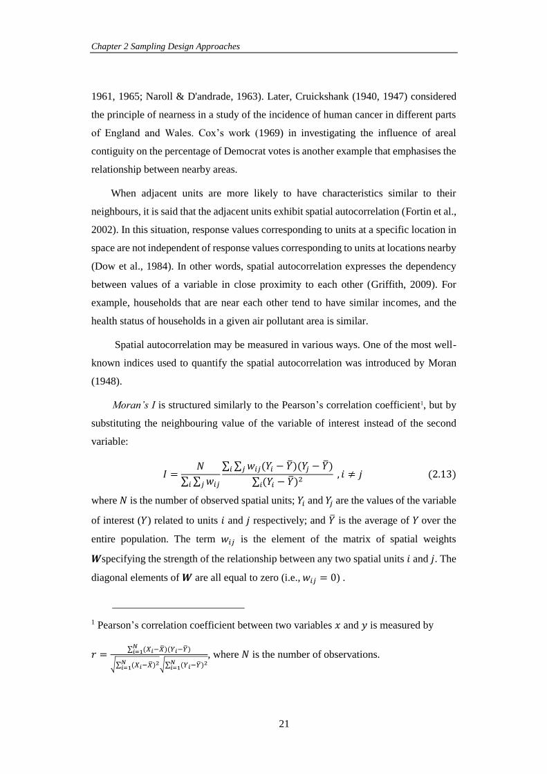
Chapter 2 Sampling Design Approaches
21
1961, 1965; Naroll & D'andrade, 1963). Later, Cruickshank (1940, 1947) considered
the principle of nearness in a study of the incidence of human cancer in different parts
of England and Wales. Cox’s work (1969) in investigating the influence of areal
contiguity on the percentage of Democrat votes is another example that emphasises the
relationship between nearby areas.
When adjacent units are more likely to have characteristics similar to their
neighbours, it is said that the adjacent units exhibit spatial autocorrelation (Fortin et al.,
2002). In this situation, response values corresponding to units at a specific location in
space are not independent of response values corresponding to units at locations nearby
(Dow et al., 1984). In other words, spatial autocorrelation expresses the dependency
between values of a variable in close proximity to each other (Griffith, 2009). For
example, households that are near each other tend to have similar incomes, and the
health status of households in a given air pollutant area is similar.
Spatial autocorrelation may be measured in various ways. One of the most well-
known indices used to quantify the spatial autocorrelation was introduced by Moran
(1948).
Moran’s I is structured similarly to the Pearson’s correlation coefficient1, but by
substituting the neighbouring value of the variable of interest instead of the second
variable:
𝐼 =𝑁
∑ ∑ 𝑤𝑖𝑗𝑗𝑖
∑ ∑ 𝑤𝑖𝑗(𝑌𝑖 − ��)(𝑌𝑗 − ��)𝑗𝑖
∑ (𝑌𝑖 − ��)2
𝑖
, 𝑖 ≠ 𝑗 (2.13)
where 𝑁 is the number of observed spatial units; 𝑌𝑖 and 𝑌𝑗 are the values of the variable
of interest (𝑌) related to units 𝑖 and 𝑗 respectively; and �� is the average of 𝑌 over the
entire population. The term 𝑤𝑖𝑗 is the element of the matrix of spatial weights
𝑾specifying the strength of the relationship between any two spatial units 𝑖 and 𝑗. The
diagonal elements of 𝑾 are all equal to zero (i.e., 𝑤𝑖𝑗 = 0) .
1 Pearson’s correlation coefficient between two variables 𝑥 and 𝑦 is measured by
𝑟 =∑ (𝑋𝑖−��)(𝑌𝑖−��)𝑁𝑖=1
√∑ (𝑋𝑖−��)2𝑁
𝑖=1 √∑ (𝑌𝑖−��)2𝑁
𝑖=1
, where 𝑁 is the number of observations.
Chapter 2 Sampling Design Approaches
22
There are a number of ways to define the weights matrix 𝑾 via similarity
measures. Generally, it is defined using contiguity between units. The two most
common forms of contiguity in spatial studies are “rook” and “queen” definitions of
neighbours. In the rook relationship, the units that share a common boundary with the
unit of interest are considered neighbours of that unit, whereas a queen relationship
means that the units adjacent via either side or corner are the unit’s neighbours. As
another option, the weights matrix 𝑊 may represents the inverse distance between
units.
The value of Moran's I usually lies between −1 and +1, but sometimes falls
outside that range (Legendre & Fortin, 1989). Under the assumption that the data are
independent and identically distributed normal random variates, Moran's I is
asymptotically normally distributed and, under the null hypothesis of no spatial
autocorrelation, its expectation is (𝐼) = −1
𝑁−1 , which tends to zero as 𝑁 increases.
Positive spatial autocorrelation is indicated by values greater than 𝐸(𝐼), whereas values
less than 𝐸(𝐼) imply negative spatial autocorrelation (Griffith, 1987).
In Chapter 4 of this thesis I will use the Moran’s I index in order to characterise
synthetic populations with different levels of spatial autocorrelation. Moran’s I will
also be employed in Chapter 5 to describe the spatial autocorrelation among units of
the population under study.
2.6.1 Review of Some Spatially Balanced Sampling Methods
In the presence of spatial autocorrelation, neighbouring units tend to have similar
values of the variable of interest and therefore provide little additional information.
Spatially balanced sampling methods are sampling designs that avoid selecting
neighbouring units in the same sample. These sampling methods, which are popular in
environmental studies, can improve the efficiency of population estimates by selecting
a sample with few nearby units (Theobald et al., 2007). Here, some well-known
spatially balanced sampling methods which are used in the next chapters are reviewed.
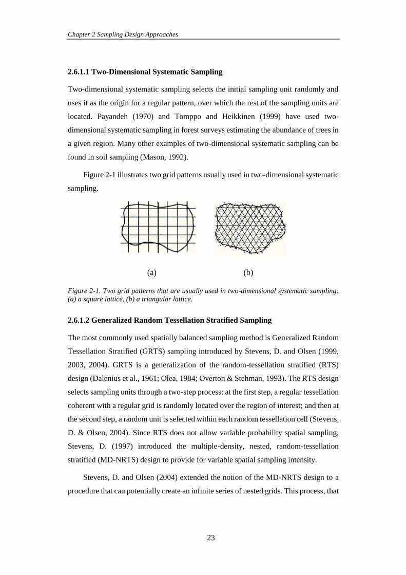
Chapter 2 Sampling Design Approaches
23
2.6.1.1 Two-Dimensional Systematic Sampling
Two-dimensional systematic sampling selects the initial sampling unit randomly and
uses it as the origin for a regular pattern, over which the rest of the sampling units are
located. Payandeh (1970) and Tomppo and Heikkinen (1999) have used two-
dimensional systematic sampling in forest surveys estimating the abundance of trees in
a given region. Many other examples of two-dimensional systematic sampling can be
found in soil sampling (Mason, 1992).
Figure 2-1 illustrates two grid patterns usually used in two-dimensional systematic
sampling.
Figure 2-1. Two grid patterns that are usually used in two-dimensional systematic sampling: (a) a square lattice, (b) a triangular lattice.
2.6.1.2 Generalized Random Tessellation Stratified Sampling
The most commonly used spatially balanced sampling method is Generalized Random
Tessellation Stratified (GRTS) sampling introduced by Stevens, D. and Olsen (1999,
2003, 2004). GRTS is a generalization of the random-tessellation stratified (RTS)
design (Dalenius et al., 1961; Olea, 1984; Overton & Stehman, 1993). The RTS design
selects sampling units through a two-step process: at the first step, a regular tessellation
coherent with a regular grid is randomly located over the region of interest; and then at
the second step, a random unit is selected within each random tessellation cell (Stevens,
D. & Olsen, 2004). Since RTS does not allow variable probability spatial sampling,
Stevens, D. (1997) introduced the multiple-density, nested, random-tessellation
stratified (MD-NRTS) design to provide for variable spatial sampling intensity.
Stevens, D. and Olsen (2004) extended the notion of the MD-NRTS design to a
procedure that can potentially create an infinite series of nested grids. This process, that
(a) (b)
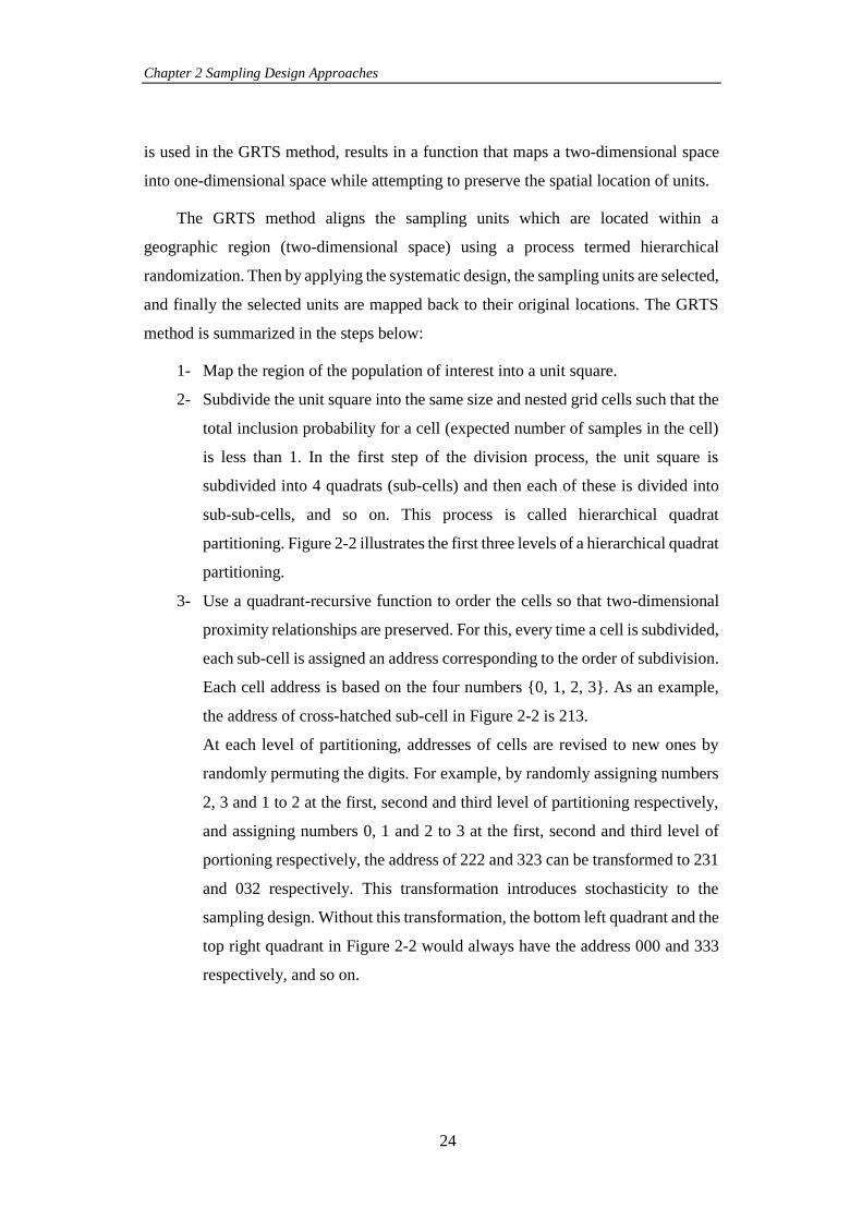
Chapter 2 Sampling Design Approaches
24
is used in the GRTS method, results in a function that maps a two-dimensional space
into one-dimensional space while attempting to preserve the spatial location of units.
The GRTS method aligns the sampling units which are located within a
geographic region (two-dimensional space) using a process termed hierarchical
randomization. Then by applying the systematic design, the sampling units are selected,
and finally the selected units are mapped back to their original locations. The GRTS
method is summarized in the steps below:
1- Map the region of the population of interest into a unit square.
2- Subdivide the unit square into the same size and nested grid cells such that the
total inclusion probability for a cell (expected number of samples in the cell)
is less than 1. In the first step of the division process, the unit square is
subdivided into 4 quadrats (sub-cells) and then each of these is divided into
sub-sub-cells, and so on. This process is called hierarchical quadrat
partitioning. Figure 2-2 illustrates the first three levels of a hierarchical quadrat
partitioning.
3- Use a quadrant-recursive function to order the cells so that two-dimensional
proximity relationships are preserved. For this, every time a cell is subdivided,
each sub-cell is assigned an address corresponding to the order of subdivision.
Each cell address is based on the four numbers {0, 1, 2, 3}. As an example,
the address of cross-hatched sub-cell in Figure 2-2 is 213.
At each level of partitioning, addresses of cells are revised to new ones by
randomly permuting the digits. For example, by randomly assigning numbers
2, 3 and 1 to 2 at the first, second and third level of partitioning respectively,
and assigning numbers 0, 1 and 2 to 3 at the first, second and third level of
portioning respectively, the address of 222 and 323 can be transformed to 231
and 032 respectively. This transformation introduces stochasticity to the
sampling design. Without this transformation, the bottom left quadrant and the
top right quadrant in Figure 2-2 would always have the address 000 and 333
respectively, and so on.
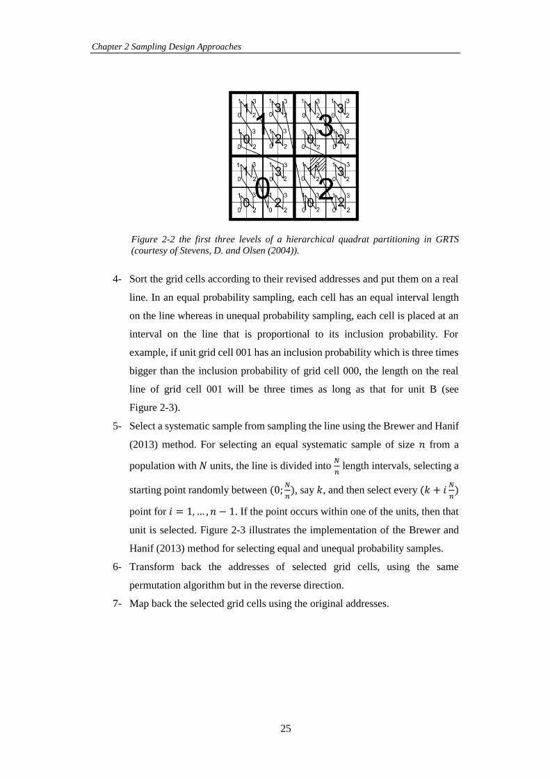
Chapter 2 Sampling Design Approaches
25
Figure 2-2 the first three levels of a hierarchical quadrat partitioning in GRTS
(courtesy of Stevens, D. and Olsen (2004)).
4- Sort the grid cells according to their revised addresses and put them on a real
line. In an equal probability sampling, each cell has an equal interval length
on the line whereas in unequal probability sampling, each cell is placed at an
interval on the line that is proportional to its inclusion probability. For
example, if unit grid cell 001 has an inclusion probability which is three times
bigger than the inclusion probability of grid cell 000, the length on the real
line of grid cell 001 will be three times as long as that for unit B (see
Figure 2-3).
5- Select a systematic sample from sampling the line using the Brewer and Hanif
(2013) method. For selecting an equal systematic sample of size 𝑛 from a
population with 𝑁 units, the line is divided into 𝑁
𝑛 length intervals, selecting a
starting point randomly between (0;𝑁
𝑛), say 𝑘, and then select every (𝑘 + 𝑖
𝑁
𝑛)
point for 𝑖 = 1, … , 𝑛 − 1. If the point occurs within one of the units, then that
unit is selected. Figure 2-3 illustrates the implementation of the Brewer and
Hanif (2013) method for selecting equal and unequal probability samples.
6- Transform back the addresses of selected grid cells, using the same
permutation algorithm but in the reverse direction.
7- Map back the selected grid cells using the original addresses.
Chapter 2 Sampling Design Approaches
26
Figure 2-3 implementation of the Brewer and Hanif (2013) method for selecting equal and unequal probability samples.
2.6.1.3 Spatially Correlated Poisson Sampling
A few years after introducing GRTS, Grafström (2012) presented a method called
spatially correlated Poisson sampling (SCPS). Grafström’s design is based on that
proposed by Bondesson and Thorburn (2008), termed correlated Poisson sampling
(CPS). CPS is a list sequential PPS sampling method that is suitable for real-time
sampling (Meister, 2004). In real time sampling, the units of the population are visited
by the sampler one by one in some order. It is a decision to be made by the sampler at
the visit whether the unit should be sampled. In real time sampling, there is no
probability of revisiting units at a later time. For implementing a list sequential method
in a population in which the units are labelled 1 to 𝑁 (according to the order they are
visited or some other order), the sampling outcome (i.e., in terms of including or
excluding the unit in the sample) is first decided for the unit labelled 1, then for the unit
labelled 2 and so forth. In fact, the sample selection process is done at several steps so
that after selecting a unit at each step the inclusion probabilities of the remaining units
are updated.
By considering distances between units, rather than just having an ordered list of
the units, Grafström (2012) adapted the CPS method to SCPS. By considering distances
000
001
002
003
Equal probability sampling Unequal probability sampling
…
331
332
333
000
001
002
003
…
332
333
Chapter 2 Sampling Design Approaches
27
between units it aims to create a negative correlation between the inclusion
probabilities of units that are close to each other.
In CPS, the first unit is sampled with probability 𝜋1 and if it is included in the
sample, 𝑈1 = 1, otherwise 𝑈1 = 0. When unit 𝑗 − 1 has been visited and the value (0
or 1) of the sampling indicator 𝑈𝑗−1 has been recorded, the inclusion probabilities for
all the remaining units are updated. The updated probabilities are denoted 𝜋𝑖(𝑗−1)
, 𝑖 ≥ 𝑗
and unit 𝑗 is then sampled with probability 𝜋𝑗(𝑗−1)
.
Let 𝜋𝑖(0)(= 𝜋𝑖) be a predefined (initial) inclusion probability of unit 𝑖 and let
𝜋𝑖(𝑗−1)
, 𝑖 ≥ 𝑗 be the updated inclusion probability of unit 𝑖 when unit 𝑗 − 1 has been
visited. Let, in the 𝑗𝑡ℎoutcome, 𝑈1, 𝑈2, … , 𝑈𝑗 corresponding to the 1𝑠𝑡 to 𝑗𝑡ℎ unit
respectively have been defined such that 𝑈𝑘 𝑘 = 1,… , 𝑗 is equal to 1 if the 𝑘𝑡ℎunit was
included in sample and 0 otherwise. Having this information, 𝜋𝑖(𝑗)
can be calculated
using Equation (2.14) below:
𝜋𝑖(𝑗)= 𝜋𝑖
(𝑗−1)− (𝑈𝑗 − 𝜋𝑗
(𝑗−1))𝑤𝑖−𝑗
(𝑖) 𝑖 ≥ 𝑗 + 1; 𝑗 = 1, 2 , … (2.14)
where 𝑤𝑖−𝑗(𝑖)
are the weights given to units 𝑖 = 𝑗 + 1, 𝑗 + 2, . . . , 𝑁 by unit 𝑗.
In SCPS, Grafström introduced “maximal weights” and “Gaussian preliminary
weights” as two different methods for assigning weights that express the distances
between units.
In the maximal weight strategy, in the 𝑗𝑡ℎ step, the unit 𝑗 gives the largest weight
to the closest unit among the units 𝑖 = 𝑗 + 1, 𝑗 + 2, … ,𝑁. Then, the second closest
unit to the 𝑗𝑡ℎ unit receives the next largest weight, and so on, with the restriction that
the sum of the weights equals unity (∑wi = 1). For units with equal distances, the
weights are distributed equally.
In the Gaussian preliminary weights strategy, some preliminary weights with sum
1 are associated with the units. The preliminary weights are controlled by a Gaussian
distribution centred at the position of unit 𝑗 as below:
𝑤𝑗(𝑖)∗ ∝ 𝑒𝑥𝑝(−(𝑑(𝑖, 𝑗) 𝜎⁄ )2) , 𝑖 = 𝑗 + 1, 𝑗 + 2, . . . , 𝑁 (2.15)
Chapter 2 Sampling Design Approaches
28
where w𝑗(i)∗
is the preliminary weight given to unit 𝑖 by unit 𝑗, 𝜎 is a parameter that can
control the spread of weights and can be chosen according to the distance between
units, and 𝑑(𝑖, 𝑗) is the distance between units 𝑖 and 𝑗. In this strategy, the biggest
weight is allocated to the nearest unit, so one option for choosing σ is the average (or
median) of the distances between each unit and its closest neighbour (Grafström, 2012).
2.6.1.4 Local Pivotal Methods
In addition to SCPS, Grafström et al. (2012) proposed two other spatial sampling
methods – local pivotal methods 1 and 2 (LPM1 and LPM2). These methods are based
on the pivotal method (PM) presented by Deville and Tille (1998). In LPMs the
population units’ inclusion probabilities are updated iteratively until 𝑛 units have
inclusion probabilities equal to 1. The main idea of these methods is to create a negative
correlation between the inclusion probabilities of close units. In this way, the
probability of selecting adjacent units together in a sample is decreased.
The pivotal method in each step of sample selection modifies the inclusion
probabilities of only two units. So, for a population of size 𝑁, a sample is obtained by
updating the inclusion probabilities in 𝑁 steps at most. The process of updating
continues until the inclusion probabilities of all the units equal either 1 or 0. When the
inclusion probability of a unit is updated to either 1 or 0, this unit is “finished”
(Grafström et al., 2012).
If 𝜋𝑖 and 𝜋𝑗 are inclusion probabilities of the 𝑖𝑡ℎ and 𝑗𝑡ℎ unit respectively, the PM
rule produces ��𝑖 and ��𝑗 as updated inclusion probabilities according to the following
rule:
Chapter 2 Sampling Design Approaches
29
if πi + πj < 1, then
(��𝑖 , ��𝑗) =
{
(0, πi + πj) with probability πj
πi + πj
(πi + πj, 0) with probability πi
πi + πj
and if πi + πj ≥ 1, then (2.16)
(��𝑖, ��𝑗) =
{
(1, πi + πj − 1) with probability
1 − πj
2 − πi − πj
(πi + πj − 1,1) with probability 1 − πi
2 − πi − πj.
At the first step, at least one of the units is finished. Finished units are not allowed
to be chosen in the next step, so the problem of sample selection is reduced to a
population with size of at most 𝑁 − 1 units at the second step. Recall that the updating
process is repeated until all of the inclusion probabilities are changed to either 0 or 1.
The process of selecting a sample by LPM1 is as follows:
a) Randomly choose one unit 𝑖.
b) Choose unit 𝑗, a nearest neighbour to 𝑖. If two or more units have the same
distance to 𝑖, then randomly choose one of them with equal probability.
c) If 𝑗 has 𝑖 as its nearest neighbour, then update the inclusion probabilities
of units 𝑖 and 𝑗 according to Equation (2.16). Otherwise go to (a).
d) If all units are finished, then stop. Otherwise go to (a).
The process of selecting a sample by LPM2 is similar to the process of LPM1, but
in this method it is not necessary to find out whether unit 𝑖 is the nearest neighbour of
unit 𝑗. In LPM2, (c) is removed from the process and the inclusion probabilities of both
units 𝑖 and 𝑗 are directly updated.
Of the two strategies for selecting sampling units introduced by Grafström et al.
(2012), LPM1 produces a more spatially balanced sample, whereas LPM2 is simpler
and faster.
In the LPM algorithm, after selecting the unit 𝑖 randomly, finding unit 𝑗, the
nearest neighbour to 𝑖 among the entire population is a computationally intensive
process. The expected number of computations needed to select a sample by LPMs is
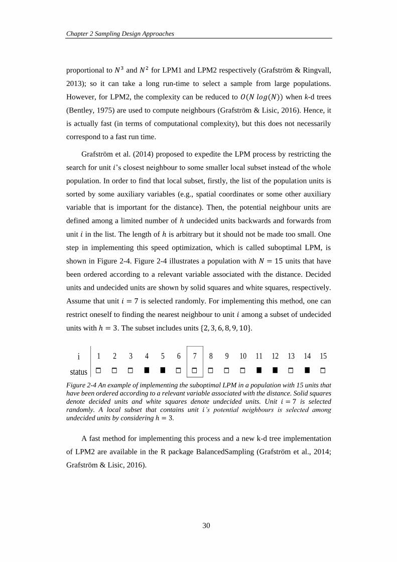
Chapter 2 Sampling Design Approaches
30
proportional to 𝑁3 and 𝑁2 for LPM1 and LPM2 respectively (Grafström & Ringvall,
2013); so it can take a long run-time to select a sample from large populations.
However, for LPM2, the complexity can be reduced to 𝑂(𝑁 𝑙𝑜𝑔(𝑁)) when k-d trees
(Bentley, 1975) are used to compute neighbours (Grafström & Lisic, 2016). Hence, it
is actually fast (in terms of computational complexity), but this does not necessarily
correspond to a fast run time.
Grafström et al. (2014) proposed to expedite the LPM process by restricting the
search for unit 𝑖’s closest neighbour to some smaller local subset instead of the whole
population. In order to find that local subset, firstly, the list of the population units is
sorted by some auxiliary variables (e.g., spatial coordinates or some other auxiliary
variable that is important for the distance). Then, the potential neighbour units are
defined among a limited number of ℎ undecided units backwards and forwards from
unit 𝑖 in the list. The length of ℎ is arbitrary but it should not be made too small. One
step in implementing this speed optimization, which is called suboptimal LPM, is
shown in Figure 2-4. Figure 2-4 illustrates a population with 𝑁 = 15 units that have
been ordered according to a relevant variable associated with the distance. Decided
units and undecided units are shown by solid squares and white squares, respectively.
Assume that unit 𝑖 = 7 is selected randomly. For implementing this method, one can
restrict oneself to finding the nearest neighbour to unit 𝑖 among a subset of undecided
units with ℎ = 3. The subset includes units {2, 3, 6, 8, 9, 10}.
Figure 2-4 An example of implementing the suboptimal LPM in a population with 15 units that
have been ordered according to a relevant variable associated with the distance. Solid squares
denote decided units and white squares denote undecided units. Unit 𝑖 = 7 is selected
randomly. A local subset that contains unit 𝑖’s potential neighbours is selected among
undecided units by considering ℎ = 3.
A fast method for implementing this process and a new k-d tree implementation
of LPM2 are available in the R package BalancedSampling (Grafström et al., 2014;
Grafström & Lisic, 2016).
i 1 2 3 4 5 6 7 8 9 10 11 12 13 14 15
status
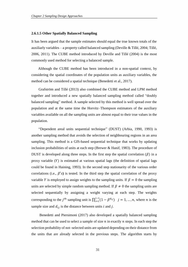
Chapter 2 Sampling Design Approaches
31
2.6.1.5 Other Spatially Balanced Sampling
It has been argued that the sample estimates should equal the true known totals of the
auxiliarly variables – a property called balanced sampling (Deville & Tillé, 2004; Tillé,
2006, 2011). The CUBE method introduced by Deville and Tillé (2004) is the most
commonly used method for selecting a balanced sample.
Although the CUBE method has been introduced in a non-spatial context, by
considering the spatial coordinates of the population units as auxiliary variables, the
method can be considered a spatial technique (Benedetti et al., 2017).
Grafström and Tillé (2013) also combined the CUBE method and LPM method
together and introduced a new spatially balanced sampling method called “doubly
balanced sampling” method. A sample selected by this method is well spread over the
population and at the same time the Horvitz–Thompson estimators of the auxiliary
variables available on all the sampling units are almost equal to their true values in the
population.
“Dependent areal units sequential technique” (DUST) (Arbia, 1990, 1993) is
another sampling method that avoids the selection of neighbouring regions in an area
sampling. This method is a GIS-based sequential technique that works by updating
inclusion probabilities of units at each step (Brewer & Hanif, 1983). The procedure of
DUST is developed along three steps. In the first step the spatial correlation (𝛽) in a
proxy variable (𝑌) is estimated at various spatial lags (the definition of spatial lags
could be found in Haining, 1993). In the second step stationarity of the various order
correlations (i.e., 𝛽′𝑠) is tested. In the third step the spatial correlation of the proxy
variable 𝑌 is employed to assign weights to the sampling units. If 𝛽 = 0 the sampling
units are selected by simple random sampling method. If 𝛽 ≠ 0 the sampling units are
selected sequentially by assigning a weight varying at each step. The weights
corresponding to the 𝑗𝑡ℎ sampling unit is ∏ (1 − 𝛽𝑑𝑖𝑗)𝑗−1𝑖=1 𝑗 = 1, … , 𝑛, where 𝑛 is the
sample size and 𝑑𝑖𝑗 is the distance between units 𝑖 and 𝑗.
Benedetti and Piersimoni (2017) also developed a spatially balanced sampling
method that can be used to select a sample of size 𝑛 in exactly 𝑛 steps. In each step the
selection probability of not–selected units are updated depending on their distance from
the units that are already selected in the previous steps. The algorithm starts by
Chapter 2 Sampling Design Approaches
32
randomly selecting a unit 𝑖 with equal probability from the population
(𝑈 = {1, 2,… , 𝑁}). Then, at every step where 𝑡 ≤ 𝑛, the algorithm updates the
selection probabilities of every other units of the population according to
𝜋𝑗𝑡 =
𝜋𝑗𝑡−1��𝑖𝑗
∑ 𝜋𝑗𝑡−1��𝑖𝑗𝑗∈𝑈
(2.17)
where 𝜋𝑗𝑡−1 is the selection probability of the unit 𝑗 at step 𝑡 − 1, and ��𝑖𝑗 is an
appropriate transformation applied to the distance matrix (𝐷𝑈 = {𝑑𝑖𝑗; 𝑖, 𝑗 = 1, … , 𝑁}).
The transformation is considered in order to standardize the distance matrix to have
known and fixed products by row ∏ 𝑑𝑖𝑗𝑖≠𝑗,𝑖∈𝑈 and column ∏ 𝑑𝑖𝑗𝑖≠𝑗,𝑖∈𝑈 .
2.6.2 Parameter Estimation in Spatially Balanced Sampling Methods
In spatially balanced sampling methods, the population total can be estimated by a
standard design-based estimator such as the HT estimator given in Equation (2.3).
However, the Sen–Yates–Grundy estimator given in Equation (2.5) for estimating the
variance of the HT estimator in spatially balanced sampling methods may be unstable
because the second order inclusion probabilities of neighbouring units are often zero or
near to zero (Robertson et al., 2013). In these cases, Stevens, D. and Olsen (2004)
presented an estimator called the “local mean variance” estimator, which is a contrast-
based estimator (Yates, 1953; Overton & Stehman, 1993; Wolter, 2007). This estimator
was first developed to estimate the variance for the GRTS method, and it has more
recently been used to compute the variance estimators for other spatially balanced
sampling methods.
The local mean variance estimator is given by:
VNBH(��𝑇) =∑∑wij ( yjπ𝑗⁄ − yDi)
2
j∈Di𝑖∈𝑠
(2.18)
where 𝐷𝑖 is a neighbourhood to unit 𝑖, containing at least four units, ��𝐷𝑖 is the total
responses of units that are located in the neighbourhood of unit 𝑖, and 𝑤𝑖𝑗 are weights
that decrease as the distance between units 𝑖 and 𝑗 increase and satisfy ∑ 𝑤𝑖𝑗𝑗∈𝐷𝑖= 1.
More details about computing the weights (𝑤𝑖𝑗) can be found in Stevens, D. and Olsen
(2003).
Chapter 2 Sampling Design Approaches
33
2.6.3 Spatial Coverage
As mentioned earlier, much of the interest in using spatially balanced sampling
methods is spreading the sample over the population and avoiding the selection of
neighboring units. Spatial balance can be measured and tested in different ways. This
section briefly reviews some techniques that will be used in the next chapters to test the
spatial coverage of a sample.
2.6.3.1 Spatial Point Pattern Analysis
A spatial point pattern analysis provides statistical methods to study the spatial
arrangements of units in the region of the population of interest. Study of spatial point
patterns has a long history and its applications appear widely in many different areas
of study (Ripley, 1977, Getis, 1984, Upton & Fingleton, 1985). This thesis uses some
of the methods in an exploration of spatial point patterns to evaluate the spatial pattern
of selected sampling units.
Generally, the spatial point pattern analysis methods are classified into quadrat-
based and distance-based methods. Quadrat-based methods are based on overlaying
areas of equal size on the region of the population of interest, whereas distance-based
methods develop statistics based on the distribution of distances between the sampling
and neighbouring units.
The simplest form of quadrat-based methods is the quadrat method where the
region of the population of interest is divided into some small quadrats of the same size.
Quadrats may have any desired shape, but they are usually square or circular. After
counting the frequency of sampling units in each quadrat, a test statistic can be
calculated using:
𝑇 =(𝑚 − 1)𝑠2
�� (2.19)
where 𝑚 is number of quadrats, �� and 𝑠2 are the observed average and observed
variance of the frequency of units among quadrats, respectively. To test the departure
from complete spatial randomness, 𝑇 can be compared to a 𝜒2 distribution with 𝑚− 1
degrees of freedom.
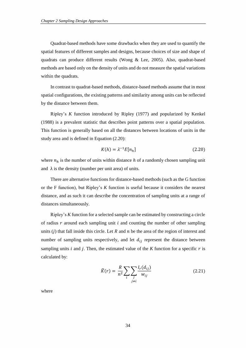
Chapter 2 Sampling Design Approaches
34
Quadrat-based methods have some drawbacks when they are used to quantify the
spatial features of different samples and designs, because choices of size and shape of
quadrats can produce different results (Wong & Lee, 2005). Also, quadrat-based
methods are based only on the density of units and do not measure the spatial variations
within the quadrats.
In contrast to quadrat-based methods, distance-based methods assume that in most
spatial configurations, the existing patterns and similarity among units can be reflected
by the distance between them.
Ripley’s K function introduced by Ripley (1977) and popularized by Kenkel
(1988) is a prevalent statistic that describes point patterns over a spatial population.
This function is generally based on all the distances between locations of units in the
study area and is defined in Equation (2.20):
𝐾(ℎ) = 𝜆−1𝐸[𝑛ℎ] (2.20)
where 𝑛ℎ is the number of units within distance ℎ of a randomly chosen sampling unit
and λ is the density (number per unit area) of units.
There are alternative functions for distance-based methods (such as the G function
or the F function), but Ripley’s K function is useful because it considers the nearest
distance, and as such it can describe the concentration of sampling units at a range of
distances simultaneously.
Ripley’s K function for a selected sample can be estimated by constructing a circle
of radius 𝑟 around each sampling unit 𝑖 and counting the number of other sampling
units (𝑗) that fall inside this circle. Let 𝑅 and 𝑛 be the area of the region of interest and
number of sampling units respectively, and let 𝑑𝑖𝑗 represent the distance between
sampling units 𝑖 and 𝑗. Then, the estimated value of the K function for a specific 𝑟 is
calculated by:
𝐾(𝑟) = 𝑅
𝑛2∑∑
𝐼𝑟(𝑑𝑖𝑗)
𝑤𝑖𝑗𝑗𝑗≠𝑖
𝑖
(2.21)
where
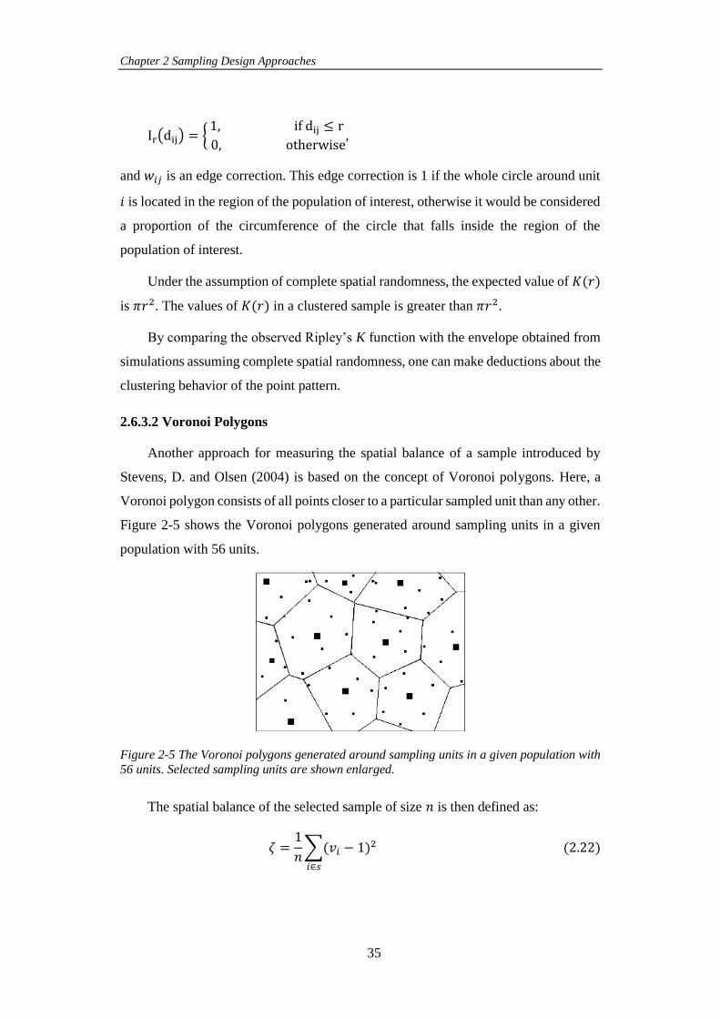
Chapter 2 Sampling Design Approaches
35
Ir(dij) = {1, if dij ≤ r
0, otherwise,
and 𝑤𝑖𝑗 is an edge correction. This edge correction is 1 if the whole circle around unit
𝑖 is located in the region of the population of interest, otherwise it would be considered
a proportion of the circumference of the circle that falls inside the region of the
population of interest.
Under the assumption of complete spatial randomness, the expected value of 𝐾(𝑟)
is 𝜋𝑟2. The values of 𝐾(𝑟) in a clustered sample is greater than 𝜋𝑟2.
By comparing the observed Ripley’s K function with the envelope obtained from
simulations assuming complete spatial randomness, one can make deductions about the
clustering behavior of the point pattern.
2.6.3.2 Voronoi Polygons
Another approach for measuring the spatial balance of a sample introduced by
Stevens, D. and Olsen (2004) is based on the concept of Voronoi polygons. Here, a
Voronoi polygon consists of all points closer to a particular sampled unit than any other.
Figure 2-5 shows the Voronoi polygons generated around sampling units in a given
population with 56 units.
Figure 2-5 The Voronoi polygons generated around sampling units in a given population with
56 units. Selected sampling units are shown enlarged.
The spatial balance of the selected sample of size 𝑛 is then defined as:
𝜁 =1
𝑛∑(𝑣𝑖 − 1)
2
𝑖∈𝑠
(2.22)
Chapter 2 Sampling Design Approaches
36
where 𝑣𝑖 indicates the sum of the inclusion probabilities of all units in the Voronoi
polygon related to the 𝑖𝑡ℎ sampling unit.
Lower values of ζ indicate a higher level of spatial balance. However, because the
range of ζ is not fixed, it can only be used in a comparative way and cannot determine
absence or presence of spatial balance in an individual sample (Tillé et al., 2017).
Recently, Tillé et al. (2017) introduced a new index based on Moran’s I that has a finite
range from −1 (perfect spatial balance) to +1 (maximum clustered), and can evaluate
the degree of spatial balance in a sample.
This thesis uses ζ as it just aims to compare the level of spatial balance among
different samples selected from the same population.
2.7 Conclusions
After introducing the concept of probability sampling, this chapter provided a
review of the relevant literature on different features of household sampling surveys.
Since the application of spatial sampling methods is a new topic in household surveys,
the properties of some common spatial methods were reviewed in this chapter. Finally,
in the last section of this chapter, some criteria that evaluate the spatial balance of the
sample were introduced.
2.8 References
Arbia, G. (1990). Sampling dependent spatial units. Paper presented at the workshop on
spatial statistics, Commission on mathematical modelling of the IGU, Boston.
Arbia, G. (1993). The use of GIS in spatial statistical surveys. International Statistical
Review/Revue Internationale de Statistique, 339-359.
Benedetti, R., & Piersimoni, F. (2017). Fast Selection of Spatially Balanced Samples. arXiv
preprint arXiv:1710.09116.
Benedetti, R., Piersimoni, F., & Postiglione, P. (2017). Spatially balanced sampling: a
review and a reappraisal. International Statistical Review, 85(3), 439-454.
Bentley, J. L. (1975). Multidimensional binary search trees used for associative searching.
Communications of the ACM, 18(9), 509-517.
Binder, D. A. (1998). Longitudinal surveys: why are these surveys different from all other
surveys? Survey Methodology, 24, 101-108.
Bondesson, L., & Thorburn, D. (2008). A list sequential sampling method suitable for real‐time sampling. Scandinavian Journal of Statistics, 35(3), 466-483.
Chapter 2 Sampling Design Approaches
37
Brewer, K. R., & Hanif, M. (1983). Sampling with unequal probabilities (Vol. 15). New
York: Springer-Verlag.
Brewer, K. R., & Hanif, M. (2013). Sampling with unequal probabilities (Vol. 15):
Springer Science & Business Media.
Chambers, R. L., & Skinner, C. J. (2003). Analysis of survey data: John Wiley & Sons.
Cochran, W. G. (1977). Sampling Techniques: 3d Ed: Wiley.
Cox, K. R. (1969). The voting decision in a spatial context. Progress in geography, 1, 81-
117.
Cruickshank, B. (1940). BA contribution towards the rational study of regional inference:
group information under random conditions. Papworth Research Bulletin, 5, 36-
81.
Cruickshank, B. (1947). Regional influences in Cancer. British journal of cancer, 1(2),
109.
Dalenius, T., Hájek, J., & Zubrzycki, S. (1961). On plane sampling and related geometrical
problems. Paper presented at the Proceedings of the 4th Berkeley symposium on
probability and mathematical statistics.
Deville, J.-C., & Tille, Y. (1998). Unequal probability sampling without replacement
through a splitting method. Biometrika, 85(1), 89-101.
Deville, J.-C., & Tillé, Y. (2004). Efficient balanced sampling: the cube method.
Biometrika, 91(4), 893-912.
Dodge, Y., & Marriott, F. (2003). International Statistical Institute. The Oxford dictionary
of statistical terms.
Dow, M. M., Burton, M. L., White, D. R., & Reitz, K. P. (1984). Galton's problem as
network autocorrelation. American Ethnologist, 754-770.
Fortin, M. J., Dale, M. R., & Ver Hoef, J. M. (2002). Spatial analysis in ecology. Wiley
StatsRef: Statistics Reference Online.
Getis, A. (1984). Interaction modeling using second-order analysis. Environment and
Planning A, 16(2), 173-183.
Grafström, A. (2012). Spatially correlated Poisson sampling. Journal of Statistical
Planning and Inference, 142(1), 139-147.
Grafström, A., & Lisic, J. (2016). BalancedSampling: Balanced and spatially balanced
sampling. R package version, 1(1).
Grafström, A., Lundström, N. L., & Schelin, L. (2012). Spatially balanced sampling
through the pivotal method. Biometrics, 68(2), 514-520.
Grafström, A., & Ringvall, A. H. (2013). Improving forest field inventories by using remote
sensing data in novel sampling designs. Canadian Journal of Forest Research,
43(11), 1015-1022.
Grafström, A., Saarela, S., & Ene, L. T. (2014). Efficient sampling strategies for forest
inventories by spreading the sample in auxiliary space. Canadian Journal of Forest
Research, 44(10), 1156-1164.
Grafström, A., & Tillé, Y. (2013). Doubly balanced spatial sampling with spreading and
restitution of auxiliary totals. Environmetrics, 24(2), 120-131.
Chapter 2 Sampling Design Approaches
38
Griffith, D. A. (1987). Spatial Autocorrelation: A Primer. Washington. DC: Association of
American Geographers.
Griffith, D. A. (2009). Spatial autocorrelation. International encyclopedia of human
geography, 2009, 308-316.
Groves, R. M., Fowler Jr, F. J., Couper, M. P., Lepkowski, J. M., Singer, E., & Tourangeau,
R. (2011). Survey methodology (Vol. 561): John Wiley & Sons.
Haining, R. (1993). Spatial data analysis in the social and environmental sciences:
Cambridge University Press.
Hájek, J. (1959). Optimal strategy and other problems in probability sampling. Časopis pro
pěstování matematiky, 84(4), 387-423.
Hansen, M. H., Hurwitz, W. N., & Madow, W. G. (1953). Sample survey methods and
theory. V. 1. Methods and applications. V. 2. Theory: John Wiley & Sons.
Harter, R., Eckman, S., English, N., & O’Muircheartaigh, C. (2010). Applied sampling for
large-scale multi-stage area probability designs: Emerald.
Horvitz, D. G., & Thompson, D. J. (1952). A generalization of sampling without
replacement from a finite universe. Journal of the American statistical Association,
47(260), 663-685.
Kenkel, N. (1988). Pattern of self‐thinning in jack pine: testing the random mortality
hypothesis. Ecology, 69(4), 1017-1024.
Kish, L. (1965). Survey sampling. New York: John Wiley and Sons.
Kish, L. (2004). Statistical design for research (Vol. 83): John Wiley & Sons.
Korn, E. L., & Graubard, B. I. (2011). Analysis of health surveys (Vol. 323): John Wiley
& Sons.
Legendre, P., & Fortin, M. J. (1989). Spatial pattern and ecological analysis. Vegetatio,
80(2), 107-138.
Lehtonen, R., & Pahkinen, E. (2004). Practical methods for design and analysis of complex
surveys: John Wiley & Sons.
Levy, P., & Lemeshow, S. (2013). Sampling of populations: methods and applications:
John Wiley & Sons.
Lohr, S. (2009). Sampling: design and analysis: Nelson Education.
Mason, B. J. (1992). Preparation of soil sampling protocols: sampling techniques and
strategies (No. PB-92-220532/XAB). Retrieved from Nevada Univ., Las Vegas,
NV (United States). Environmental Research Center.
Meister, K. (2004). On methods for real time sampling and distributions in sampling.
(Doctoral dissertation), Umeå University, Matematisk statistik.
Moran, P. A. (1948). The interpretation of statistical maps. Journal of the Royal Statistical
Society. Series B (Methodological), 10(2), 243-251.
Murphy, P. (2008). An overview of primary sampling units (PSUs) in multi-stage samples
for demographic surveys. Paper presented at the Proceedings of the American
Statistical Association, Government Statistics Section.
Naroll, R. (1961). Two solutions to Galton's problem. Philosophy of Science, 15-39.
Chapter 2 Sampling Design Approaches
39
Naroll, R. (1965). Galton's problem: The logic of cross-cultural analysis. Social Research,
428-451.
Naroll, R., & D'andrade, R. G. (1963). Two further solutions to Galton's problem. American
Anthropologist, 65(5), 1053-1067.
Neyman, J. (1934). On the two different aspects of the representative method: the method
of stratified sampling and the method of purposive selection. Journal of the Royal
Statistical Society, 97(4), 558-625.
Olea, R. A. (1984). Sampling design optimization for spatial functions. Journal of the
International Association for Mathematical Geology, 16(4), 369-392.
Overton, S. W., & Stehman, S. V. (1993). Properties of designs for sampling continuous
spatial resources from a triangular grid. Communications in Statistics--Theory and
Methods, 22(9), 251-264.
Payandeh, B. (1970). Relative efficiency of two-dimensional systematic sampling. Forest
science, 16(3), 271-276.
Pettersson, H. (2005). Design of master sampling frames and master samples for household
surveys in developing countries. In Household surveys in developing and transition
countries. UN Department of Economic and Social Affairs, Statistics Division.
Ripley, B. D. (1977). Modelling spatial patterns. Journal of the Royal Statistical Society.
Series B (Methodological), 172-212.
Robertson, B., Brown, J., McDonald, T., & Jaksons, P. (2013). BAS: balanced acceptance
sampling of natural resources. Biometrics, 69(3), 776-784.
Särndal, C.-E., Swensson, B., & Wretman, J. (2003). Model assisted survey sampling:
Springer Science & Business Media.
Skinner, C. J., Holt, D., & Smith, T. F. (1989). Analysis of complex surveys: John Wiley &
Sons.
Smith, P., Lynn, P., & Elliot, D. (2009). Sample design for longitudinal surveys.
Methodology of Longitudinal Surveys, 21-33.
Som, R. K. (1973). A manual of sampling techniques: Heinemann Educational Books.
Stats NZ. (2017). Household Labour Force Survey sources and methods: 2016. In: in April
2017 by Stats NZ Tatauranga Aotearoa Wellington, New Zealand.
Steel, D. (1997). Producing monthly estimates of unemployment and employment
according to the International Labour Office definition. Journal of the Royal
Statistical Society: Series A (Statistics in Society), 160(1), 5-46.
Steel, D., & McLaren, C. (2009). Design and analysis of surveys repeated over time. In
Handbook of Statistics (Vol. 29, pp. 289-313): Elsevier.
Stevens, D. (1997). Variable density grid‐based sampling designs for continuous spatial
populations. Environmetrics: The official journal of the International
Environmetrics Society, 8(3), 167-195.
Stevens, D., & Olsen, A. (1999). Spatially restricted surveys over time for aquatic
resources. Journal of Agricultural, Biological, and Environmental Statistics, 415-
428.
Chapter 2 Sampling Design Approaches
40
Stevens, D., & Olsen, A. (2003). Variance estimation for spatially balanced samples of
environmental resources. Environmetrics, 14(6), 593-610.
Stevens, D., & Olsen, A. (2004). Spatially balanced sampling of natural resources. Journal
of the American statistical Association, 99(465), 262-278.
Theobald, D. M., Stevens Jr, D. L., White, D., Urquhart, N. S., Olsen, A. R., & Norman, J.
B. (2007). Using GIS to generate spatially balanced random survey designs for
natural resource applications. Environmental Management, 40(1), 134-146.
Thompson, M. (1997). Theory of sample surveys (Vol. 74): CRC Press.
Thurgood, L., Walter, E., Carter, G., Henn, S., Huang, G., Nooter, D., Smith, W., Cash, R.
W., Salvucci, S., & Seastrom, M. (2003). NCES Handbook of Survey Methods:
Technical Report.
Tillé, Y. (2006). Sampling algorithms: Springer.
Tillé, Y. (2011). Ten years of balanced sampling with the cube method: an appraisal. Survey
Methodology, 37(2), 215-226.
Tillé, Y., Dickson, M. M., Espa, G., & Giuliani, D. (2017). Measuring the spatial balance
of a sample: A new measure based on the Moran's I index. arXiv preprint
arXiv:1710.04549.
Tomppo, E., & Heikkinen, J. (1999). National forest inventory of Finland—past, present
and future. Statistics, registries and research-experiences from Finland, 89-108.
Tschuprow, A. A. (1923). On the mathematical expectation of the moments of frequency
distributions in the case of correlated observations (Chapters 4-6). Metron, 2, 646-
683.
Tylor, E. B. (1889). On a method of investigating the development of institutions; applied
to laws of marriage and descent. The Journal of the Anthropological Institute of
Great Britain and Ireland, 18, 245-272.
United Nations-Statistical Division. (2008). Designing household survey samples:
practical guidelines (Vol. 98): United Nations Publications.
United States Bureau of the Census. (2000). Current Population Survey: Design and
Methodology (Vol. 63): US Department of Commerce, Bureau of the Census.
Upton, G., & Fingleton, B. (1985). Spatial data analysis by example. Volume 1: Point
pattern and quantitative data: John Wiley & Sons Ltd.
Valliant, R., Dever, J. A., & Kreuter, F. (2013). Practical tools for designing and weighting
survey samples: Springer.
Wolter, K. (2007). Introduction to variance estimation: Springer Science & Business
Media.
Wong, W., & Lee, J. (2005). Statistical analysis of geographic information with ArcView
GIS and ArcGIS: Wiley.
Wright, T. (2001). Selected moments in the development of probability sampling: theory
and practice. Paper presented at the Survey research methods section newsletter.
Yansaneh, I. S. (2005). Overview of sample design issues for household surveys in
developing and transition countries. In Household sample surveys in developing

Chapter 2 Sampling Design Approaches
41
and transition countries. UN Department of Economic and Social Affairs,
Statistics Division.
Yates, F. (1953). Sampling methods for censuses and surveys. Sampling methods for
censuses and surveys.(2nd ed).
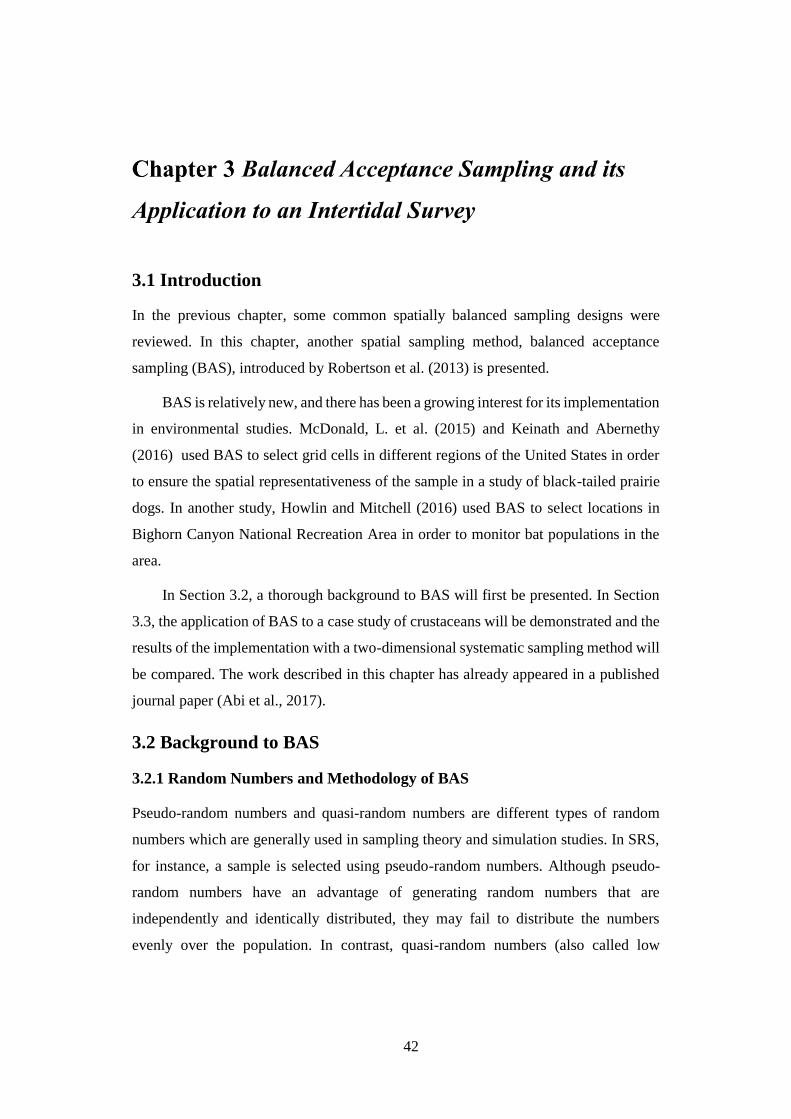
42
Balanced Acceptance Sampling and its
Application to an Intertidal Survey
3.1 Introduction
In the previous chapter, some common spatially balanced sampling designs were
reviewed. In this chapter, another spatial sampling method, balanced acceptance
sampling (BAS), introduced by Robertson et al. (2013) is presented.
BAS is relatively new, and there has been a growing interest for its implementation
in environmental studies. McDonald, L. et al. (2015) and Keinath and Abernethy
(2016) used BAS to select grid cells in different regions of the United States in order
to ensure the spatial representativeness of the sample in a study of black-tailed prairie
dogs. In another study, Howlin and Mitchell (2016) used BAS to select locations in
Bighorn Canyon National Recreation Area in order to monitor bat populations in the
area.
In Section 3.2, a thorough background to BAS will first be presented. In Section
3.3, the application of BAS to a case study of crustaceans will be demonstrated and the
results of the implementation with a two-dimensional systematic sampling method will
be compared. The work described in this chapter has already appeared in a published
journal paper (Abi et al., 2017).
3.2 Background to BAS
3.2.1 Random Numbers and Methodology of BAS
Pseudo-random numbers and quasi-random numbers are different types of random
numbers which are generally used in sampling theory and simulation studies. In SRS,
for instance, a sample is selected using pseudo-random numbers. Although pseudo-
random numbers have an advantage of generating random numbers that are
independently and identically distributed, they may fail to distribute the numbers
evenly over the population. In contrast, quasi-random numbers (also called low
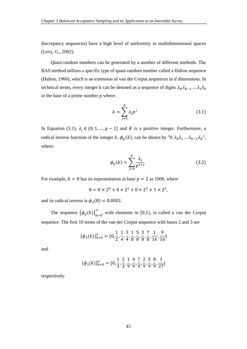
Chapter 3 Balanced Acceptance Sampling and its Application to an Intertidal Survey
43
discrepancy sequences) have a high level of uniformity in multidimensional spaces
(Levy, G., 2002).
Quasi-random numbers can be generated by a number of different methods. The
BAS method utilizes a specific type of quasi-random number called a Halton sequence
(Halton, 1960), which is an extension of van der Corput sequences in 𝑑 dimensions. In
technical terms, every integer k can be denoted as a sequence of digits 𝜆𝐾𝜆𝐾−1…𝜆1𝜆0
in the base of a prime number p where:
𝑘 =∑𝜆𝑗𝑝𝑗
𝐾
𝑗=0
(3.1)
In Equation (3.1), 𝜆𝑗 ∈ {0, 1, … , 𝑝 − 1} and 𝐾 is a positive integer. Furthermore, a
radical inverse function of the integer 𝑘, 𝜙𝑝(𝑘), can be shown by "0. 𝜆0𝜆1…𝜆𝐾−1𝜆𝐾",
where:
𝜙𝑝(𝑘) =∑𝜆𝑗𝑝1+𝑗
𝐾
𝑗=0
(3.2)
For example, 𝑘 = 8 has its representation in base 𝑝 = 2 as 1000, where
8 = 0 × 20 + 0 × 21 + 0 × 22 + 1 × 23,
and its radical inverse is 𝜙2(8) = 0.0001.
The sequence {𝜙𝑝(𝑘)}𝑘=0∞
, with elements in [0,1), is called a van der Corput
sequence. The first 10 terms of the van der Corput sequence with bases 2 and 3 are
{𝜙2(𝑘)}𝑘=09 = {0,
1
2,1
4,3
4,1
8,5
8,3
8,7
8,1
16,9
16}
and
{𝜙3(𝑘)}𝑘=09 = {0,
1
3,2
3,1
9,4
9,7
9,2
9,5
9,8
9,1
27}
respectively.
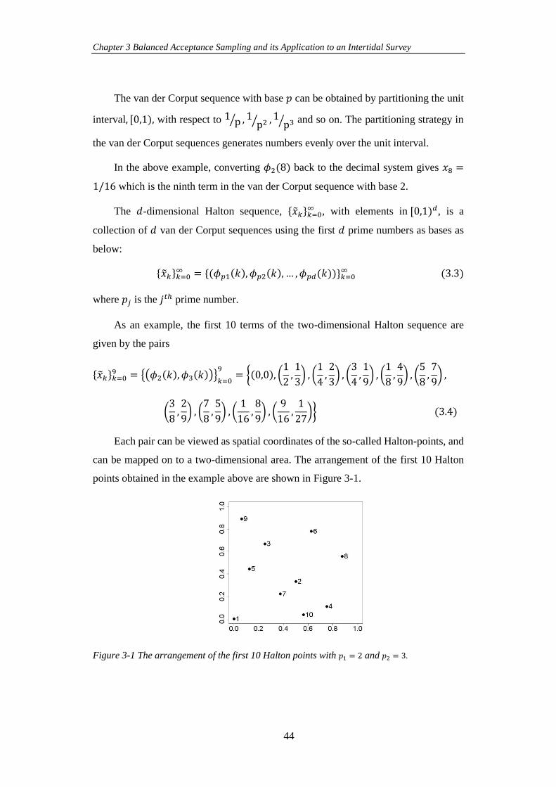
Chapter 3 Balanced Acceptance Sampling and its Application to an Intertidal Survey
44
The van der Corput sequence with base 𝑝 can be obtained by partitioning the unit
interval, [0,1), with respect to 1 p⁄ , 1 p2⁄ , 1 p3⁄ and so on. The partitioning strategy in
the van der Corput sequences generates numbers evenly over the unit interval.
In the above example, converting 𝜙2(8) back to the decimal system gives 𝑥8 =
1/16 which is the ninth term in the van der Corput sequence with base 2.
The 𝑑-dimensional Halton sequence, {��𝑘}𝑘=0∞ , with elements in [0,1)𝑑, is a
collection of 𝑑 van der Corput sequences using the first 𝑑 prime numbers as bases as
below:
{��𝑘}𝑘=0∞ = {(𝜙𝑝1(𝑘), 𝜙𝑝2(𝑘),… , 𝜙𝑝𝑑(𝑘))}𝑘=0
∞ (3.3)
where 𝑝𝑗 is the 𝑗𝑡ℎ prime number.
As an example, the first 10 terms of the two-dimensional Halton sequence are
given by the pairs
{��𝑘}𝑘=09 = {(𝜙2(𝑘), 𝜙3(𝑘))}𝑘=0
9= {(0,0), (
1
2,1
3) , (
1
4,2
3) , (
3
4,1
9) , (
1
8,4
9) , (
5
8,7
9) ,
(3
8,2
9) , (
7
8,5
9) , (
1
16,8
9) , (
9
16,1
27)} (3.4)
Each pair can be viewed as spatial coordinates of the so-called Halton-points, and
can be mapped on to a two-dimensional area. The arrangement of the first 10 Halton
points obtained in the example above are shown in Figure 3-1.
Figure 3-1 The arrangement of the first 10 Halton points with 𝑝1 = 2 and 𝑝2 = 3.
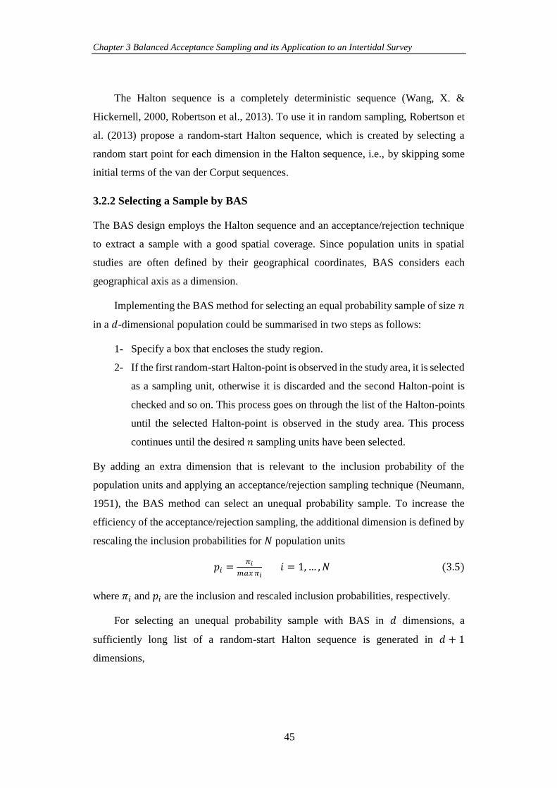
Chapter 3 Balanced Acceptance Sampling and its Application to an Intertidal Survey
45
The Halton sequence is a completely deterministic sequence (Wang, X. &
Hickernell, 2000, Robertson et al., 2013). To use it in random sampling, Robertson et
al. (2013) propose a random-start Halton sequence, which is created by selecting a
random start point for each dimension in the Halton sequence, i.e., by skipping some
initial terms of the van der Corput sequences.
3.2.2 Selecting a Sample by BAS
The BAS design employs the Halton sequence and an acceptance/rejection technique
to extract a sample with a good spatial coverage. Since population units in spatial
studies are often defined by their geographical coordinates, BAS considers each
geographical axis as a dimension.
Implementing the BAS method for selecting an equal probability sample of size 𝑛
in a 𝑑-dimensional population could be summarised in two steps as follows:
1- Specify a box that encloses the study region.
2- If the first random-start Halton-point is observed in the study area, it is selected
as a sampling unit, otherwise it is discarded and the second Halton-point is
checked and so on. This process goes on through the list of the Halton-points
until the selected Halton-point is observed in the study area. This process
continues until the desired 𝑛 sampling units have been selected.
By adding an extra dimension that is relevant to the inclusion probability of the
population units and applying an acceptance/rejection sampling technique (Neumann,
1951), the BAS method can select an unequal probability sample. To increase the
efficiency of the acceptance/rejection sampling, the additional dimension is defined by
rescaling the inclusion probabilities for 𝑁 population units
𝑝𝑖 =𝜋𝑖
𝑚𝑎𝑥𝜋𝑖 𝑖 = 1, … , 𝑁 (3.5)
where 𝜋𝑖 and 𝑝𝑖 are the inclusion and rescaled inclusion probabilities, respectively.
For selecting an unequal probability sample with BAS in 𝑑 dimensions, a
sufficiently long list of a random-start Halton sequence is generated in 𝑑 + 1
dimensions,
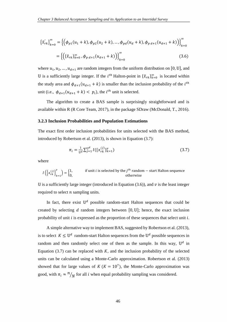
Chapter 3 Balanced Acceptance Sampling and its Application to an Intertidal Survey
46
{��𝑟𝑘 }𝑘=0∞
= {(𝜙𝑝1(𝑢1 + 𝑘), 𝜙𝑝2(𝑢2 + 𝑘),… ,𝜙𝑝𝑑(𝑢𝑑 + 𝑘), 𝜙𝑝 𝑑+1(𝑢𝑑+1 + 𝑘))}𝑘=0
∞
= {({��𝑟𝑘}𝑘=0∞ , 𝜙𝑝 𝑑+1(𝑢𝑑+1 + 𝑘))}
𝑘=0
∞
(3.6)
where 𝑢1, 𝑢2, … , 𝑢𝑑+1 are random integers from the uniform distribution on [0, 𝕌], and
𝕌 is a sufficiently large integer. If the 𝑖𝑡ℎ Halton-point in {��𝑟𝑘}𝑘=0∞ is located within
the study area and 𝜙𝑑+1(𝑢𝑑+1 + 𝑘) is smaller than the inclusion probability of the 𝑖𝑡ℎ
unit (i.e., 𝜙𝑑+1(𝑢𝑑+1 + 𝑘) < 𝑝𝑖), the 𝑖𝑡ℎ unit is selected.
The algorithm to create a BAS sample is surprisingly straightforward and is
available within R (R Core Team, 2017), in the package SDraw (McDonald, T., 2016).
3.2.3 Inclusion Probabilities and Population Estimations
The exact first order inclusion probabilities for units selected with the BAS method,
introduced by Robertson et al. (2013), is shown in Equation (3.7):
𝜋𝑖 =1
𝕌𝑑∑ 𝐼({𝑥𝑟𝑘
(𝑗)}𝑘=1𝑣 )𝕌𝑑
𝑗=1 (3.7)
where
𝐼 ({𝑥𝑟𝑘(𝑗)}𝑘=1
𝑣
) = {1, if unit 𝑖 is selected by the 𝑗𝑡ℎ random − start Halton sequence0, otherwise
𝕌 is a sufficiently large integer (introduced in Equation (3.6)), and 𝑣 is the least integer
required to select 𝑛 sampling units.
In fact, there exist 𝕌𝑑 possible random-start Halton sequences that could be
created by selecting 𝑑 random integers between [0, 𝕌]; hence, the exact inclusion
probability of unit 𝑖 is expressed as the proportion of these sequences that select unit 𝑖.
A simple alternative way to implement BAS, suggested by Robertson et al. (2013),
is to select 𝐾 ≤ 𝕌𝑑 random-start Halton sequences from the 𝕌𝑑 possible sequences in
random and then randomly select one of them as the sample. In this way, 𝕌𝑑 in
Equation (3.7) can be replaced with 𝐾, and the inclusion probability of the selected
units can be calculated using a Monte-Carlo approximation. Robertson et al. (2013)
showed that for large values of 𝐾 (𝐾 = 107), the Monte-Carlo approximation was
good, with 𝜋𝑖 ≈𝑛𝑁⁄ for all 𝑖 when equal probability sampling was considered.
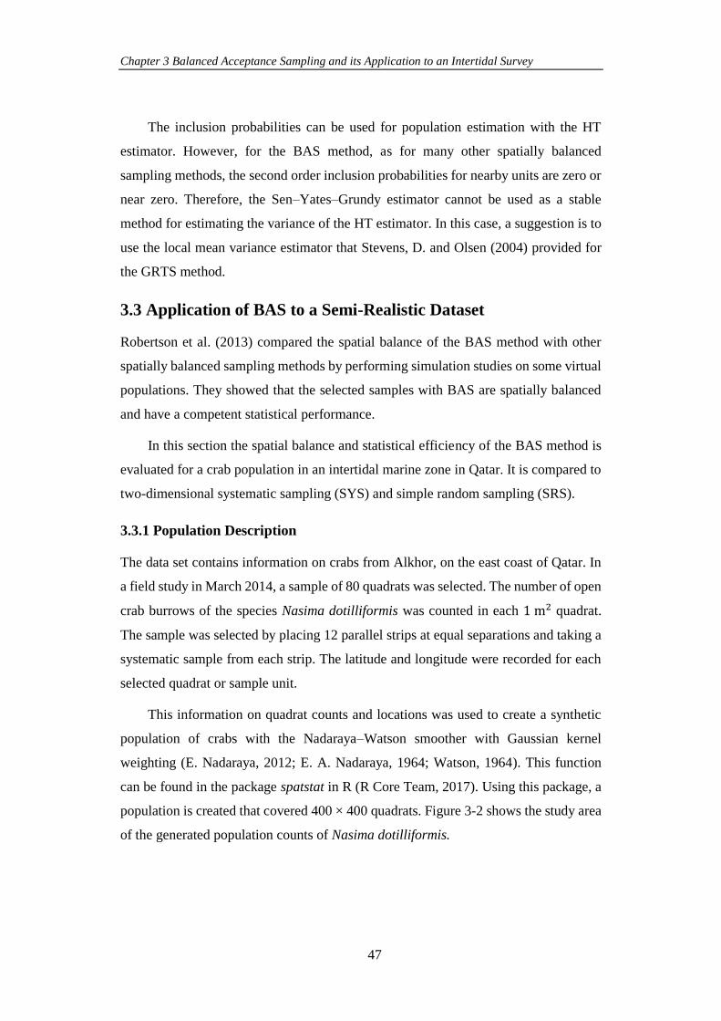
Chapter 3 Balanced Acceptance Sampling and its Application to an Intertidal Survey
47
The inclusion probabilities can be used for population estimation with the HT
estimator. However, for the BAS method, as for many other spatially balanced
sampling methods, the second order inclusion probabilities for nearby units are zero or
near zero. Therefore, the Sen–Yates–Grundy estimator cannot be used as a stable
method for estimating the variance of the HT estimator. In this case, a suggestion is to
use the local mean variance estimator that Stevens, D. and Olsen (2004) provided for
the GRTS method.
3.3 Application of BAS to a Semi-Realistic Dataset
Robertson et al. (2013) compared the spatial balance of the BAS method with other
spatially balanced sampling methods by performing simulation studies on some virtual
populations. They showed that the selected samples with BAS are spatially balanced
and have a competent statistical performance.
In this section the spatial balance and statistical efficiency of the BAS method is
evaluated for a crab population in an intertidal marine zone in Qatar. It is compared to
two-dimensional systematic sampling (SYS) and simple random sampling (SRS).
3.3.1 Population Description
The data set contains information on crabs from Alkhor, on the east coast of Qatar. In
a field study in March 2014, a sample of 80 quadrats was selected. The number of open
crab burrows of the species Nasima dotilliformis was counted in each 1 m2 quadrat.
The sample was selected by placing 12 parallel strips at equal separations and taking a
systematic sample from each strip. The latitude and longitude were recorded for each
selected quadrat or sample unit.
This information on quadrat counts and locations was used to create a synthetic
population of crabs with the Nadaraya–Watson smoother with Gaussian kernel
weighting (E. Nadaraya, 2012; E. A. Nadaraya, 1964; Watson, 1964). This function
can be found in the package spatstat in R (R Core Team, 2017). Using this package, a
population is created that covered 400 × 400 quadrats. Figure 3-2 shows the study area
of the generated population counts of Nasima dotilliformis.
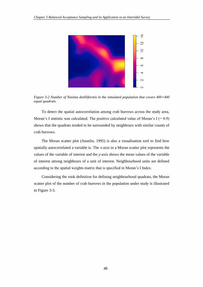
Chapter 3 Balanced Acceptance Sampling and its Application to an Intertidal Survey
48
Figure 3-2 Number of Nasima dotilliformis in the simulated population that covers 400×400
equal quadrats.
To detect the spatial autocorrelation among crab burrows across the study area,
Moran’s I statistic was calculated. The positive calculated value of Moran’s I (= 0.9)
shows that the quadrats tended to be surrounded by neighbours with similar counts of
crab burrows.
The Moran scatter plot (Anselin, 1995) is also a visualisation tool to find how
spatially autocorrelated a variable is. The x-axis in a Moran scatter plot represents the
values of the variable of interest and the y-axis shows the mean values of the variable
of interest among neighbours of a unit of interest. Neighbourhood units are defined
according to the spatial weights matrix that is specified in Moran’s I Index.
Considering the rook definition for defining neighbourhood quadrats, the Moran
scatter plot of the number of crab burrows in the population under study is illustrated
in Figure 3-3.
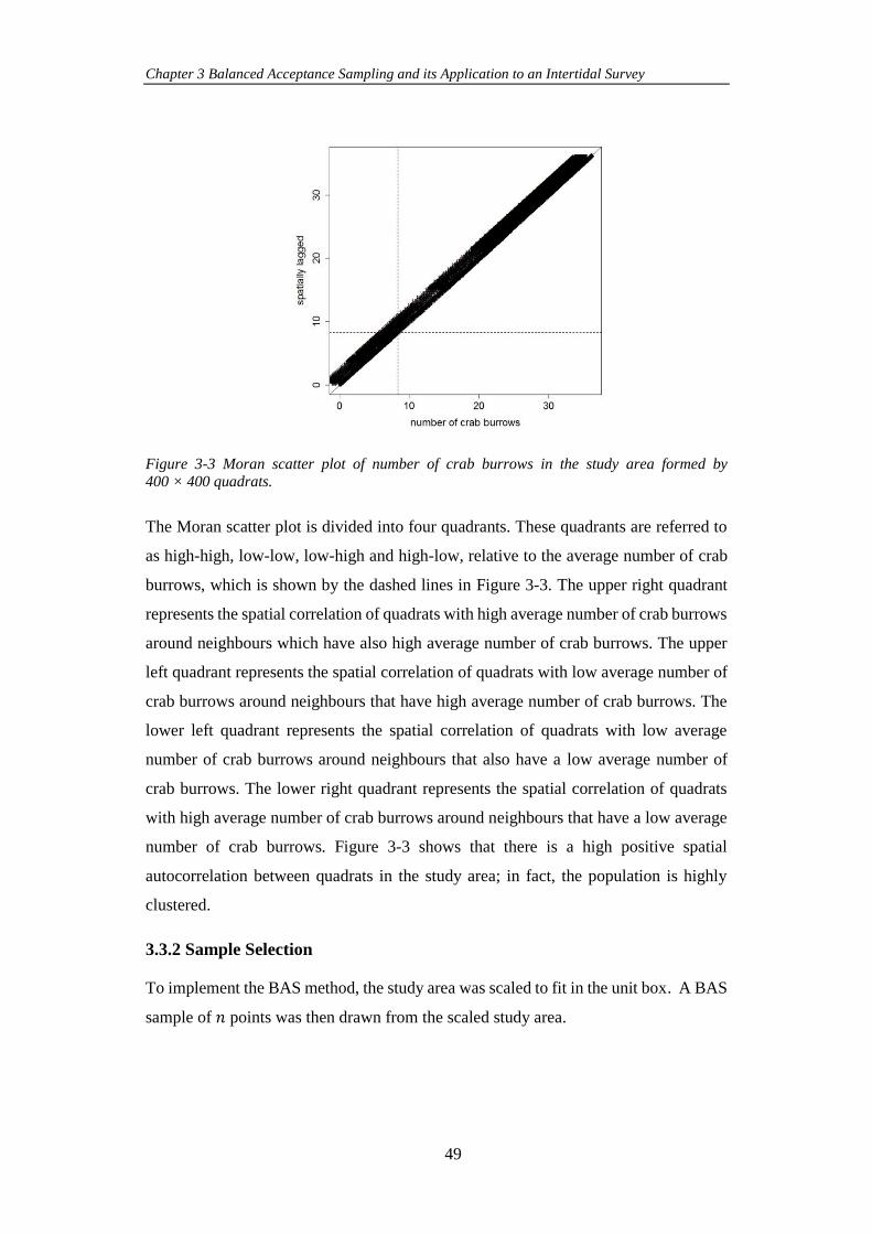
Chapter 3 Balanced Acceptance Sampling and its Application to an Intertidal Survey
49
Figure 3-3 Moran scatter plot of number of crab burrows in the study area formed by 400 × 400 quadrats.
The Moran scatter plot is divided into four quadrants. These quadrants are referred to
as high-high, low-low, low-high and high-low, relative to the average number of crab
burrows, which is shown by the dashed lines in Figure 3-3. The upper right quadrant
represents the spatial correlation of quadrats with high average number of crab burrows
around neighbours which have also high average number of crab burrows. The upper
left quadrant represents the spatial correlation of quadrats with low average number of
crab burrows around neighbours that have high average number of crab burrows. The
lower left quadrant represents the spatial correlation of quadrats with low average
number of crab burrows around neighbours that also have a low average number of
crab burrows. The lower right quadrant represents the spatial correlation of quadrats
with high average number of crab burrows around neighbours that have a low average
number of crab burrows. Figure 3-3 shows that there is a high positive spatial
autocorrelation between quadrats in the study area; in fact, the population is highly
clustered.
3.3.2 Sample Selection
To implement the BAS method, the study area was scaled to fit in the unit box. A BAS
sample of 𝑛 points was then drawn from the scaled study area.
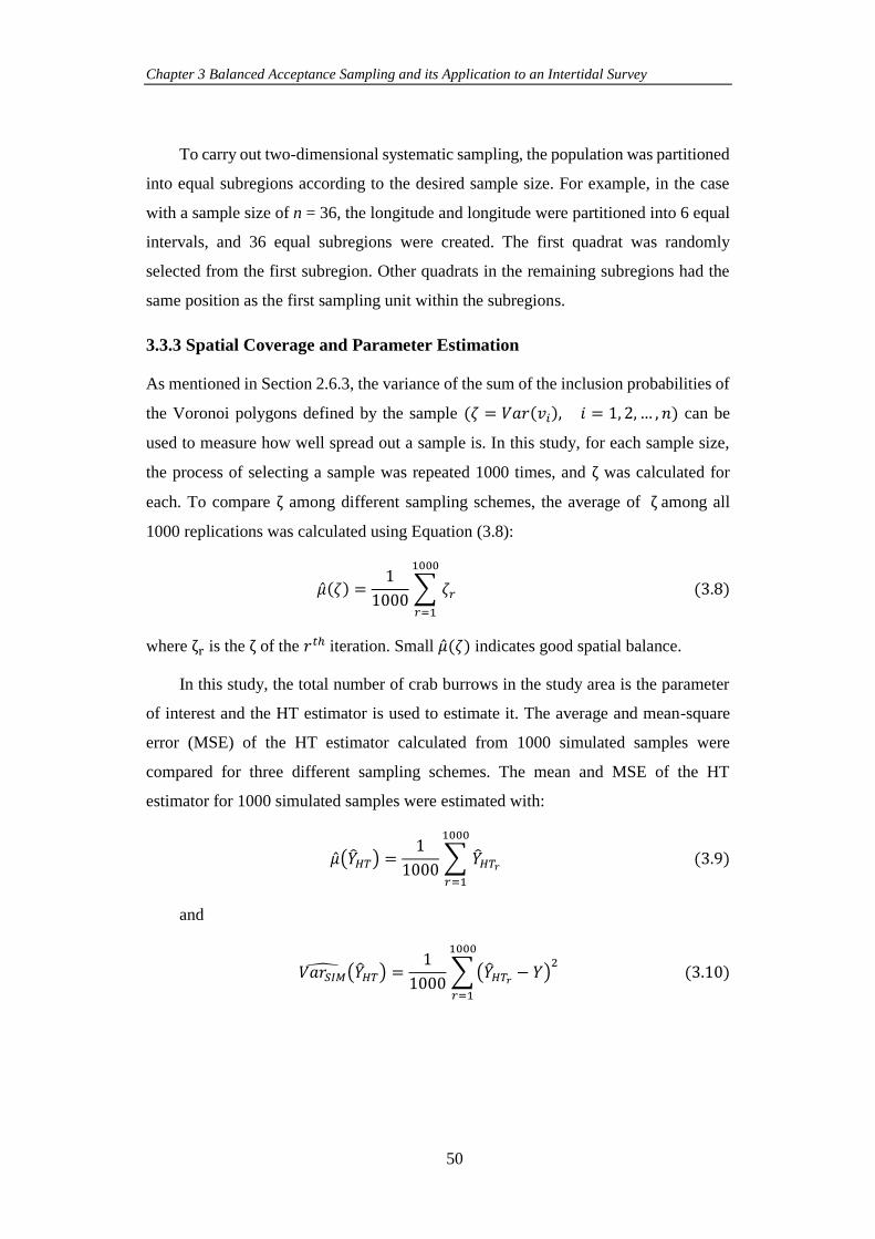
Chapter 3 Balanced Acceptance Sampling and its Application to an Intertidal Survey
50
To carry out two-dimensional systematic sampling, the population was partitioned
into equal subregions according to the desired sample size. For example, in the case
with a sample size of n = 36, the longitude and longitude were partitioned into 6 equal
intervals, and 36 equal subregions were created. The first quadrat was randomly
selected from the first subregion. Other quadrats in the remaining subregions had the
same position as the first sampling unit within the subregions.
3.3.3 Spatial Coverage and Parameter Estimation
As mentioned in Section 2.6.3, the variance of the sum of the inclusion probabilities of
the Voronoi polygons defined by the sample (𝜁 = 𝑉𝑎𝑟(𝑣𝑖), 𝑖 = 1, 2,… , 𝑛) can be
used to measure how well spread out a sample is. In this study, for each sample size,
the process of selecting a sample was repeated 1000 times, and ζ was calculated for
each. To compare ζ among different sampling schemes, the average of ζ among all
1000 replications was calculated using Equation (3.8):
��(𝜁) =1
1000∑ 𝜁𝑟
1000
𝑟=1
(3.8)
where ζr is the ζ of the 𝑟𝑡ℎ iteration. Small ��(𝜁) indicates good spatial balance.
In this study, the total number of crab burrows in the study area is the parameter
of interest and the HT estimator is used to estimate it. The average and mean-square
error (MSE) of the HT estimator calculated from 1000 simulated samples were
compared for three different sampling schemes. The mean and MSE of the HT
estimator for 1000 simulated samples were estimated with:
��(��𝐻𝑇) =1
1000∑ ��𝐻𝑇𝑟
1000
𝑟=1
(3.9)
and
𝑉𝑎𝑟𝑆𝐼��(��𝐻𝑇) =1
1000∑(��𝐻𝑇𝑟 − 𝑌)
21000
𝑟=1
(3.10)
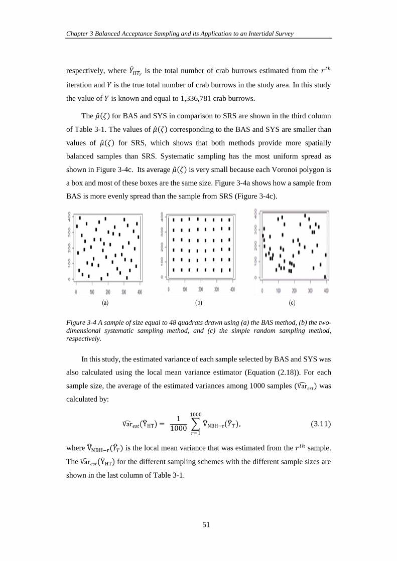
Chapter 3 Balanced Acceptance Sampling and its Application to an Intertidal Survey
51
respectively, where ��𝐻𝑇𝑟 is the total number of crab burrows estimated from the 𝑟𝑡ℎ
iteration and 𝑌 is the true total number of crab burrows in the study area. In this study
the value of 𝑌 is known and equal to 1,336,781 crab burrows.
The ��(𝜁) for BAS and SYS in comparison to SRS are shown in the third column
of Table 3-1. The values of ��(𝜁) corresponding to the BAS and SYS are smaller than
values of ��(𝜁) for SRS, which shows that both methods provide more spatially
balanced samples than SRS. Systematic sampling has the most uniform spread as
shown in Figure 3-4c. Its average ��(𝜁) is very small because each Voronoi polygon is
a box and most of these boxes are the same size. Figure 3-4a shows how a sample from
BAS is more evenly spread than the sample from SRS (Figure 3-4c).
Figure 3-4 A sample of size equal to 48 quadrats drawn using (a) the BAS method, (b) the two-
dimensional systematic sampling method, and (c) the simple random sampling method, respectively.
In this study, the estimated variance of each sample selected by BAS and SYS was
also calculated using the local mean variance estimator (Equation (2.18)). For each
sample size, the average of the estimated variances among 1000 samples (Var𝑒𝑠𝑡) was
calculated by:
Var𝑒𝑠𝑡(YHT) = 1
1000 ∑ VNBH−r(��𝑇)
1000
𝑟=1
, (3.11)
where VNBH−r(��𝑇) is the local mean variance that was estimated from the 𝑟𝑡ℎ sample.
The Var𝑒𝑠𝑡(YHT) for the different sampling schemes with the different sample sizes are
shown in the last column of Table 3-1.
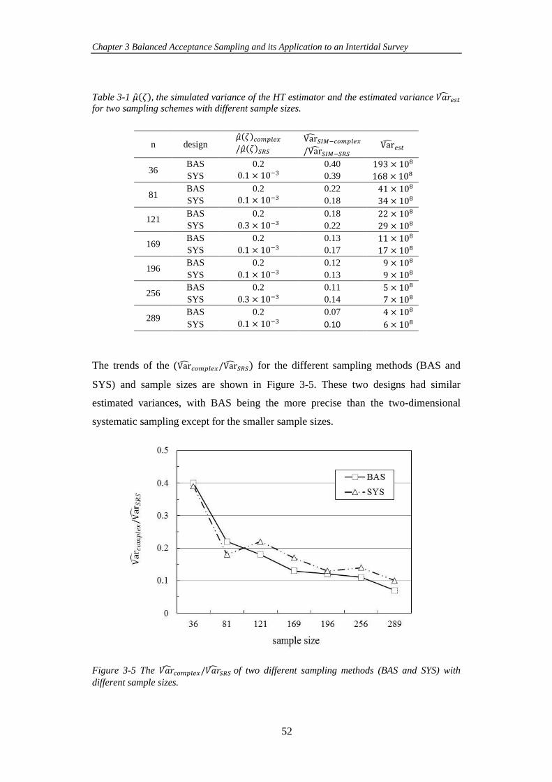
Chapter 3 Balanced Acceptance Sampling and its Application to an Intertidal Survey
52
Table 3-1 ��(𝜁), the simulated variance of the HT estimator and the estimated variance 𝑉𝑎��𝑒𝑠𝑡 for two sampling schemes with different sample sizes.
n design ��(𝜁)𝑐𝑜𝑚𝑝𝑙𝑒𝑥/��(𝜁)𝑆𝑅𝑆
Var𝑆𝐼𝑀−𝑐𝑜𝑚𝑝𝑙𝑒𝑥/Var𝑆𝐼𝑀−𝑆𝑅𝑆
Var𝑒𝑠𝑡
36 BAS 0.2 0.40 193 × 108
SYS 0.1 × 10⁻³ 0.39 168 × 108
81 BAS 0.2 0.22 41 × 108
SYS 0.1 × 10⁻³ 0.18 34 × 108
121 BAS 0.2 0.18 22 × 108
SYS 0.3 × 10⁻³ 0.22 29 × 108
169 BAS 0.2 0.13 11 × 108
SYS 0.1 × 10⁻³ 0.17 17 × 108
196 BAS 0.2 0.12 9 × 10⁸
SYS 0.1 × 10⁻³ 0.13 9 × 10⁸
256 BAS 0.2 0.11 5 × 10⁸
SYS 0.3 × 10⁻³ 0.14 7 × 10⁸
289 BAS 0.2 0.07 4 × 10⁸
SYS 0.1 × 10⁻³ 0.10 6 × 10⁸
The trends of the (Var𝑐𝑜𝑚𝑝𝑙𝑒𝑥/Var𝑆𝑅𝑆) for the different sampling methods (BAS and
SYS) and sample sizes are shown in Figure 3-5. These two designs had similar
estimated variances, with BAS being the more precise than the two-dimensional
systematic sampling except for the smaller sample sizes.
Figure 3-5 The 𝑉𝑎��𝑐𝑜𝑚𝑝𝑙𝑒𝑥/𝑉𝑎��𝑆𝑅𝑆 of two different sampling methods (BAS and SYS) with
different sample sizes.
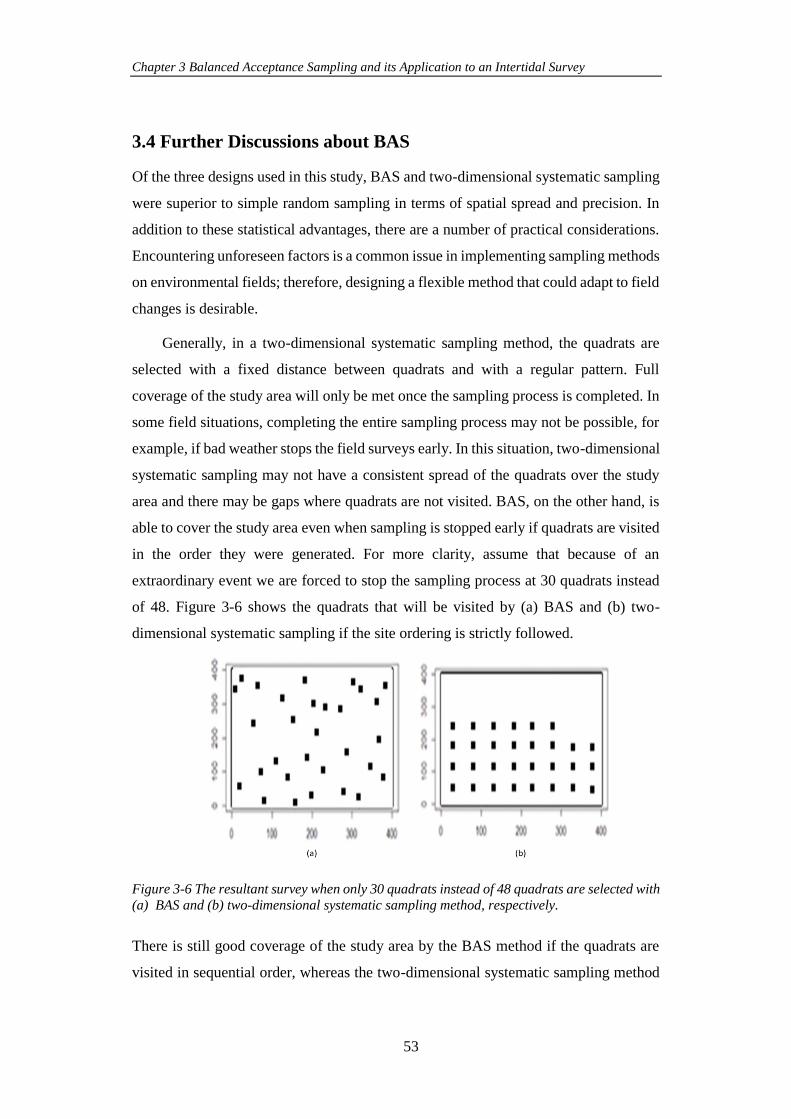
Chapter 3 Balanced Acceptance Sampling and its Application to an Intertidal Survey
53
3.4 Further Discussions about BAS
Of the three designs used in this study, BAS and two-dimensional systematic sampling
were superior to simple random sampling in terms of spatial spread and precision. In
addition to these statistical advantages, there are a number of practical considerations.
Encountering unforeseen factors is a common issue in implementing sampling methods
on environmental fields; therefore, designing a flexible method that could adapt to field
changes is desirable.
Generally, in a two-dimensional systematic sampling method, the quadrats are
selected with a fixed distance between quadrats and with a regular pattern. Full
coverage of the study area will only be met once the sampling process is completed. In
some field situations, completing the entire sampling process may not be possible, for
example, if bad weather stops the field surveys early. In this situation, two-dimensional
systematic sampling may not have a consistent spread of the quadrats over the study
area and there may be gaps where quadrats are not visited. BAS, on the other hand, is
able to cover the study area even when sampling is stopped early if quadrats are visited
in the order they were generated. For more clarity, assume that because of an
extraordinary event we are forced to stop the sampling process at 30 quadrats instead
of 48. Figure 3-6 shows the quadrats that will be visited by (a) BAS and (b) two-
dimensional systematic sampling if the site ordering is strictly followed.
Figure 3-6 The resultant survey when only 30 quadrats instead of 48 quadrats are selected with
(a) BAS and (b) two-dimensional systematic sampling method, respectively.
There is still good coverage of the study area by the BAS method if the quadrats are
visited in sequential order, whereas the two-dimensional systematic sampling method
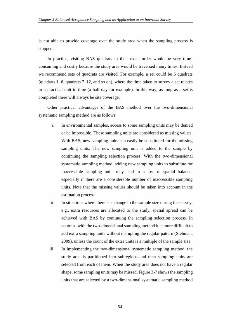
Chapter 3 Balanced Acceptance Sampling and its Application to an Intertidal Survey
54
is not able to provide coverage over the study area when the sampling process is
stopped.
In practice, visiting BAS quadrats in their exact order would be very time-
consuming and costly because the study area would be traversed many times. Instead
we recommend sets of quadrats are visited. For example, a set could be 6 quadrats
(quadrats 1–6, quadrats 7–12, and so on), where the time taken to survey a set relates
to a practical unit in time (a half-day for example). In this way, as long as a set is
completed there will always be site coverage.
Other practical advantages of the BAS method over the two-dimensional
systematic sampling method are as follows:
i. In environmental samples, access to some sampling units may be denied
or be impossible. These sampling units are considered as missing values.
With BAS, new sampling units can easily be substituted for the missing
sampling units. The new sampling unit is added to the sample by
continuing the sampling selection process. With the two-dimensional
systematic sampling method, adding new sampling units to substitute for
inaccessible sampling units may lead to a loss of spatial balance,
especially if there are a considerable number of inaccessible sampling
units. Note that the missing values should be taken into account in the
estimation process.
ii. In situations where there is a change to the sample size during the survey,
e.g., extra resources are allocated to the study, spatial spread can be
achieved with BAS by continuing the sampling selection process. In
contrast, with the two-dimensional sampling method it is more difficult to
add extra sampling units without disrupting the regular pattern (Stehman,
2009), unless the count of the extra units is a multiple of the sample size.
iii. In implementing the two-dimensional systematic sampling method, the
study area is partitioned into subregions and then sampling units are
selected from each of them. When the study area does not have a regular
shape, some sampling units may be missed. Figure 3-7 shows the sampling
units that are selected by a two-dimensional systematic sampling method
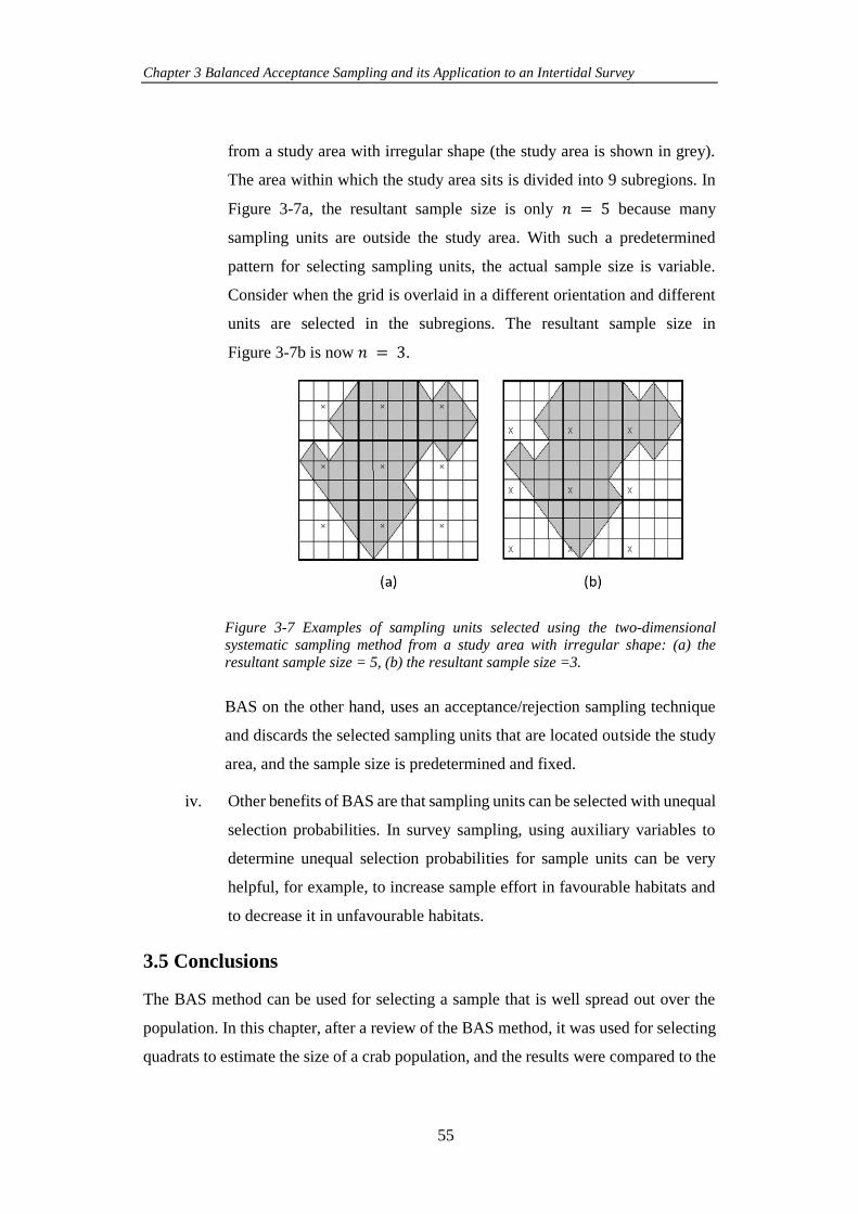
Chapter 3 Balanced Acceptance Sampling and its Application to an Intertidal Survey
55
from a study area with irregular shape (the study area is shown in grey).
The area within which the study area sits is divided into 9 subregions. In
Figure 3-7a, the resultant sample size is only 𝑛 = 5 because many
sampling units are outside the study area. With such a predetermined
pattern for selecting sampling units, the actual sample size is variable.
Consider when the grid is overlaid in a different orientation and different
units are selected in the subregions. The resultant sample size in
Figure 3-7b is now 𝑛 = 3.
Figure 3-7 Examples of sampling units selected using the two-dimensional systematic sampling method from a study area with irregular shape: (a) the
resultant sample size = 5, (b) the resultant sample size =3.
BAS on the other hand, uses an acceptance/rejection sampling technique
and discards the selected sampling units that are located outside the study
area, and the sample size is predetermined and fixed.
iv. Other benefits of BAS are that sampling units can be selected with unequal
selection probabilities. In survey sampling, using auxiliary variables to
determine unequal selection probabilities for sample units can be very
helpful, for example, to increase sample effort in favourable habitats and
to decrease it in unfavourable habitats.
3.5 Conclusions
The BAS method can be used for selecting a sample that is well spread out over the
population. In this chapter, after a review of the BAS method, it was used for selecting
quadrats to estimate the size of a crab population, and the results were compared to the
Chapter 3 Balanced Acceptance Sampling and its Application to an Intertidal Survey
56
results for a two-dimensional systematic sampling and the simple random sampling
method. Although the results for BAS and SYS were comparable, BAS has several
practical advantages, including its ability to adapt to unexpected changes in the
sampling process, which make it preferable.
3.6 References
Abi, N., Moradi, M., Salehi, M., Brown, J., Al-Khayat, J. A., & Moltchanova, E. (2017).
Application of balanced acceptance sampling to an intertidal survey. Journal of
Landscape Ecology, 10(1), 96-107.
Anselin, L. (1995). Local indicators of spatial association-LISA. Geographical Analysis,
27(2), 93-115.
Halton, J. H. (1960). On the efficiency of certain quasi-random sequences of points in
evaluating multi-dimensional integrals. Numerische Mathematik, 2(1), 84-90.
Howlin, S., & Mitchell, J. (2016). Monitoring Black-Tailed Prairie Dogs in Colorado with
the 2015 NAIP Imagery. Google Scholar.
Keinath, D. A., & Abernethy, I. (2016). Bat population monitoring of Bighorn Canyon
National Recreation Area: 2015 progress report. Prepared for the Bighorn Canyon
NRA by the Wyoming Natural Diversity Database, University of Wyoming,
Laramie, Wyoming.
Levy, G. (2002). An introduction to quasi-random numbers. Numerical Algorithms Group
Ltd., http://www. nag. co. uk/IndustryArticles/introduction_to_quasi_random_
numbers. pdf (last accessed in April 10, 2012), 143.
McDonald, L., Mitchell, J., Howlin, S., & Goodman, C. (2015). Range-wide monitoring of
Black-tailed Prairie Dogs in the United States: pilot study. Western Ecosystems
Technology Inc., Laramie, Wyoming.
McDonald, T. (2016). SDraw: Spatially balanced sample draws for spatial objects. R
package ver, 2(3).
R Core Team. (2017). R: A language and environment for statistical computing. R
Foundation for Statistical Computing, Vienna, Austria. URL https://www. R-
project. org.
Robertson, B., Brown, J., McDonald, T., & Jaksons, P. (2013). BAS: balanced acceptance
sampling of natural resources. Biometrics, 69(3), 776-784.
Stehman, S. V. (2009). Sampling designs for accuracy assessment of land cover.
International Journal of Remote Sensing, 30(20), 5243-5272.
Stevens, D., & Olsen, A. (2004). Spatially balanced sampling of natural resources. Journal
of the American statistical Association, 99(465), 262-278.
Wang, X., & Hickernell, F. J. (2000). Randomized Halton sequences. Mathematical and
Computer Modelling, 32(7-8), 887-899.
57
Population Characteristics and
Performance of Balanced Acceptance Sampling
4.1 Introduction
It is important to consider the characteristics of the population of interest during the
design of a sampling scheme. For instance, the similarity between neighbouring units
is one of the characteristics of most spatial populations and by using spatially balanced
sampling methods selection of neighbouring units in a sample can be avoided.
Although there are a number of different spatially balanced sampling methods in the
literature, their implementations have been usually for populations where the response
variables follow a continuous distribution. In contrast, there has been little discussion
on application of spatially balanced sampling methods in the cases where the response
variables are dependent binary data (e.g., the presence or absence of a characteristic).
Collecting and analysing the binary data (dichotomous responses) such as
presence or absence of children, retirees, disabled persons in the household, whether or
not the household possesses a car or has access to running water is a common task in
many social surveys. Therefore, it is helpful to consider whether using spatially
balanced sampling methods can be useful in these situations. The first part of this
chapter intends to examine whether the balanced acceptance sampling (BAS) method,
as an example of a spatially balanced sampling method, is an efficient design when the
response variable is binary.
The presence (existence) of some specific subgroups in a population is better dealt
with via the use of stratified sampling methods. Employing a stratified sampling
method ensures that the selected sample includes representation from each subgroup
(Cochran, 1977). Whilst stratified sampling is an effective sampling scheme, it can only
be implemented when the boundaries of the strata are clearly delineated. Sometimes
defining mutually exclusive strata may be a challenging process, and therefore
statisticians try to find an appropriate solution to avoid defining strata. With increasing
Chapter 4 Population Characteristics and Performance of Balanced Acceptance Sampling
58
interest in applying spatially balanced sampling methods, an important question is
whether these sampling methods can be used as an alternative to the stratified sampling.
The second part of this chapter seeks to investigate the suitability of applying BAS
in stratified sampling. It also compares the efficiency of two possible ways of applying
BAS on a stratified population.
4.2 Application of BAS on Populations With Different Spatial
Autocorrelation
Obtaining precise population estimates is one of the most important goals in selecting
a suitable sampling design. Most of the literature in the area of spatially balanced
sampling methods have emphasized that these sampling designs are more precise than
the non-spatially balanced sampling methods when there is spatial autocorrelation in
the population of interest (Stevens, D. & Olsen, 2004; Grafström et al., 2012). In this
section, we examine to what extent spatial autocorrelation affects the efficiency of
BAS.
The performance of the BAS method in populations with different levels of spatial
autocorrelation was examined through conducting simulation studies on synthetic
georeferenced populations. Each georeferenced population consisted of 100 by 100
square units, 𝑁 = 10,000. From each georeferenced population, 1000 samples were
selected using two different sampling methods (SRS and BAS), and the results were
compared. To ensure that the results were not affected by the size of the selected
samples, the sample selection process was repeated for seven different sample sizes
(𝑛 = 50, 100, 150, 200, 250, 300 and 350). In this evaluation, two types of
georeferenced populations were considered: a population where the response has a
Gaussian distribution, and a population with binary responses.
4.2.1 Using BAS in Populations Where Observations Have a Gaussian
Distribution
In this case, it was assumed that the response values came from a standard normal
distribution, 𝑁(0,1). After generating populations consisting of 10,000 observations
(100 by 100 grid), the simulation study was conducted with different variations of the
spatial features. To ensure that the results were consistent with the structure of the
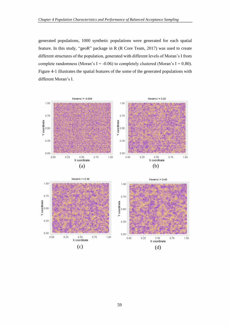
Chapter 4 Population Characteristics and Performance of Balanced Acceptance Sampling
59
generated populations, 1000 synthetic populations were generated for each spatial
feature. In this study, “geoR” package in R (R Core Team, 2017) was used to create
different structures of the population, generated with different levels of Moran’s I from
complete randomness (Moran’s I = -0.06) to completely clustered (Moran’s I = 0.80).
Figure 4-1 illustrates the spatial features of the some of the generated populations with
different Moran’s I.
(a) (b)
(c) (d)
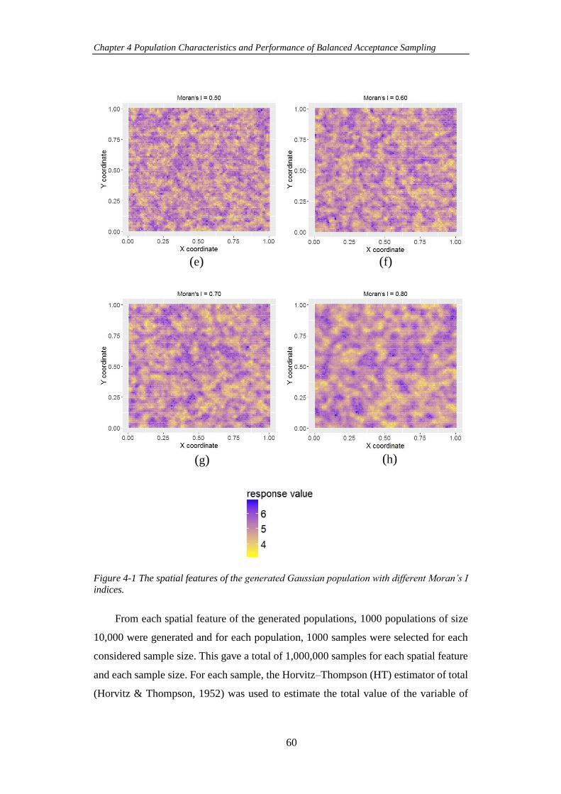
Chapter 4 Population Characteristics and Performance of Balanced Acceptance Sampling
60
Figure 4-1 The spatial features of the generated Gaussian population with different Moran’s I
indices.
From each spatial feature of the generated populations, 1000 populations of size
10,000 were generated and for each population, 1000 samples were selected for each
considered sample size. This gave a total of 1,000,000 samples for each spatial feature
and each sample size. For each sample, the Horvitz–Thompson (HT) estimator of total
(Horvitz & Thompson, 1952) was used to estimate the total value of the variable of
(e) (f)
(g) (h)
(i)
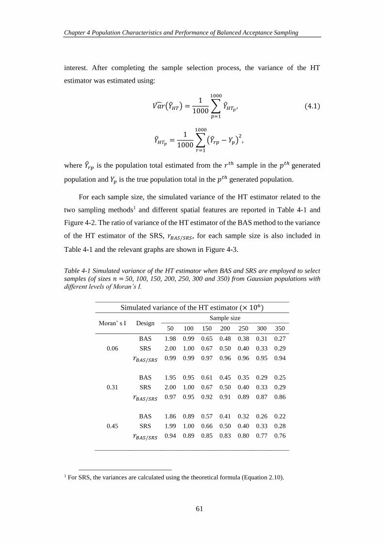
Chapter 4 Population Characteristics and Performance of Balanced Acceptance Sampling
61
interest. After completing the sample selection process, the variance of the HT
estimator was estimated using:
𝑉𝑎��(��𝐻𝑇) =1
1000∑ ��𝐻𝑇𝑝 ,
1000
𝑝=1
(4.1)
��𝐻𝑇𝑝 =1
1000∑(��𝑟𝑝 − 𝑌𝑝)
21000
𝑟=1
,
where ��𝑟𝑝 is the population total estimated from the 𝑟𝑡ℎ sample in the 𝑝𝑡ℎ generated
population and 𝑌𝑝 is the true population total in the 𝑝𝑡ℎ generated population.
For each sample size, the simulated variance of the HT estimator related to the
two sampling methods1 and different spatial features are reported in Table 4-1 and
Figure 4-2. The ratio of variance of the HT estimator of the BAS method to the variance
of the HT estimator of the SRS, 𝑟𝐵𝐴𝑆/𝑆𝑅𝑆, for each sample size is also included in
Table 4-1 and the relevant graphs are shown in Figure 4-3.
Table 4-1 Simulated variance of the HT estimator when BAS and SRS are employed to select
samples (of sizes 𝑛 = 50, 100, 150, 200, 250, 300 and 350) from Gaussian populations with
different levels of Moran’s I.
Simulated variance of the HT estimator (× 106)
Moran’ s I Design Sample size
50 100 150 200 250 300 350
BAS 1.98 0.99 0.65 0.48 0.38 0.31 0.27
0.06 SRS 2.00 1.00 0.67 0.50 0.40 0.33 0.29
𝑟𝐵𝐴𝑆/𝑆𝑅𝑆 0.99 0.99 0.97 0.96 0.96 0.95 0.94
BAS 1.95 0.95 0.61 0.45 0.35 0.29 0.25
0.31 SRS 2.00 1.00 0.67 0.50 0.40 0.33 0.29
𝑟𝐵𝐴𝑆/𝑆𝑅𝑆 0.97 0.95 0.92 0.91 0.89 0.87 0.86
BAS 1.86 0.89 0.57 0.41 0.32 0.26 0.22
0.45 SRS 1.99 1.00 0.66 0.50 0.40 0.33 0.28
𝑟𝐵𝐴𝑆/𝑆𝑅𝑆 0.94 0.89 0.85 0.83 0.80 0.77 0.76
1 For SRS, the variances are calculated using the theoretical formula (Equation 2.10).
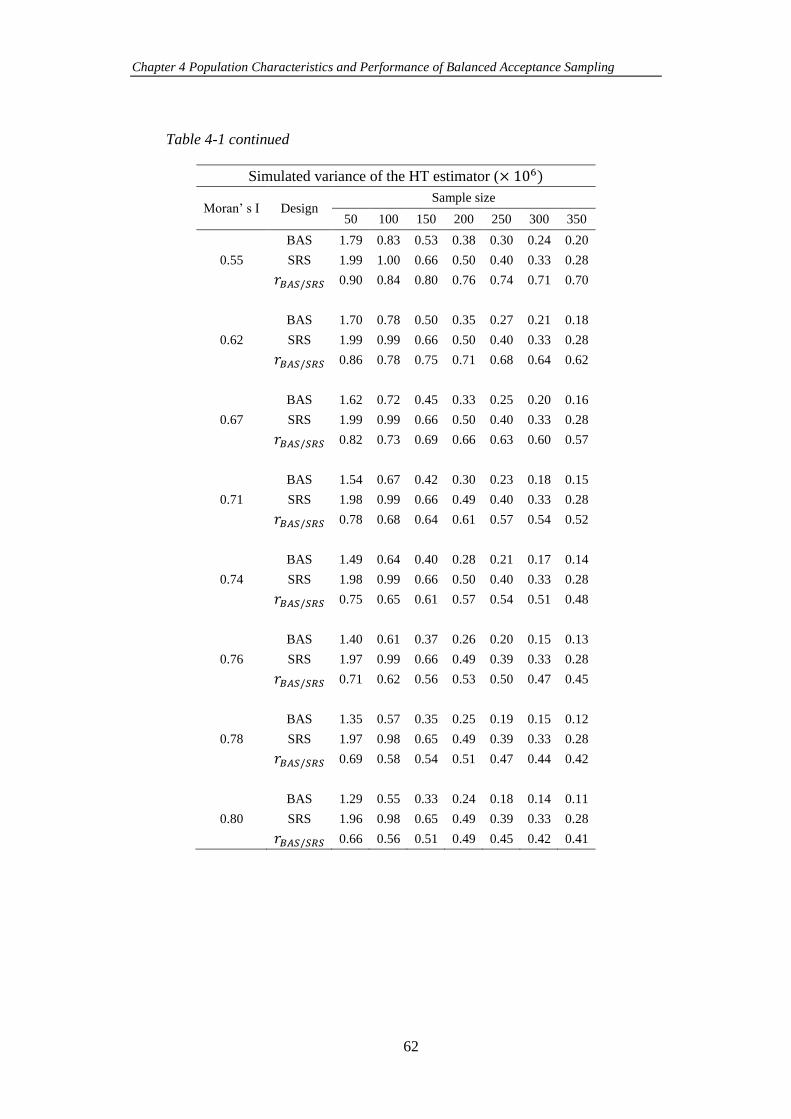
Chapter 4 Population Characteristics and Performance of Balanced Acceptance Sampling
62
Table 4-1 continued
Simulated variance of the HT estimator (× 106)
Moran’ s I Design Sample size
50 100 150 200 250 300 350
BAS 1.79 0.83 0.53 0.38 0.30 0.24 0.20
0.55 SRS 1.99 1.00 0.66 0.50 0.40 0.33 0.28
𝑟𝐵𝐴𝑆/𝑆𝑅𝑆 0.90 0.84 0.80 0.76 0.74 0.71 0.70
BAS 1.70 0.78 0.50 0.35 0.27 0.21 0.18
0.62 SRS 1.99 0.99 0.66 0.50 0.40 0.33 0.28
𝑟𝐵𝐴𝑆/𝑆𝑅𝑆 0.86 0.78 0.75 0.71 0.68 0.64 0.62
BAS 1.62 0.72 0.45 0.33 0.25 0.20 0.16
0.67 SRS 1.99 0.99 0.66 0.50 0.40 0.33 0.28
𝑟𝐵𝐴𝑆/𝑆𝑅𝑆 0.82 0.73 0.69 0.66 0.63 0.60 0.57
BAS 1.54 0.67 0.42 0.30 0.23 0.18 0.15
0.71 SRS 1.98 0.99 0.66 0.49 0.40 0.33 0.28
𝑟𝐵𝐴𝑆/𝑆𝑅𝑆 0.78 0.68 0.64 0.61 0.57 0.54 0.52
BAS 1.49 0.64 0.40 0.28 0.21 0.17 0.14
0.74 SRS 1.98 0.99 0.66 0.50 0.40 0.33 0.28
𝑟𝐵𝐴𝑆/𝑆𝑅𝑆 0.75 0.65 0.61 0.57 0.54 0.51 0.48
BAS 1.40 0.61 0.37 0.26 0.20 0.15 0.13
0.76 SRS 1.97 0.99 0.66 0.49 0.39 0.33 0.28
𝑟𝐵𝐴𝑆/𝑆𝑅𝑆 0.71 0.62 0.56 0.53 0.50 0.47 0.45
BAS 1.35 0.57 0.35 0.25 0.19 0.15 0.12
0.78 SRS 1.97 0.98 0.65 0.49 0.39 0.33 0.28
𝑟𝐵𝐴𝑆/𝑆𝑅𝑆 0.69 0.58 0.54 0.51 0.47 0.44 0.42
BAS 1.29 0.55 0.33 0.24 0.18 0.14 0.11
0.80 SRS 1.96 0.98 0.65 0.49 0.39 0.33 0.28
𝑟𝐵𝐴𝑆/𝑆𝑅𝑆 0.66 0.56 0.51 0.49 0.45 0.42 0.41
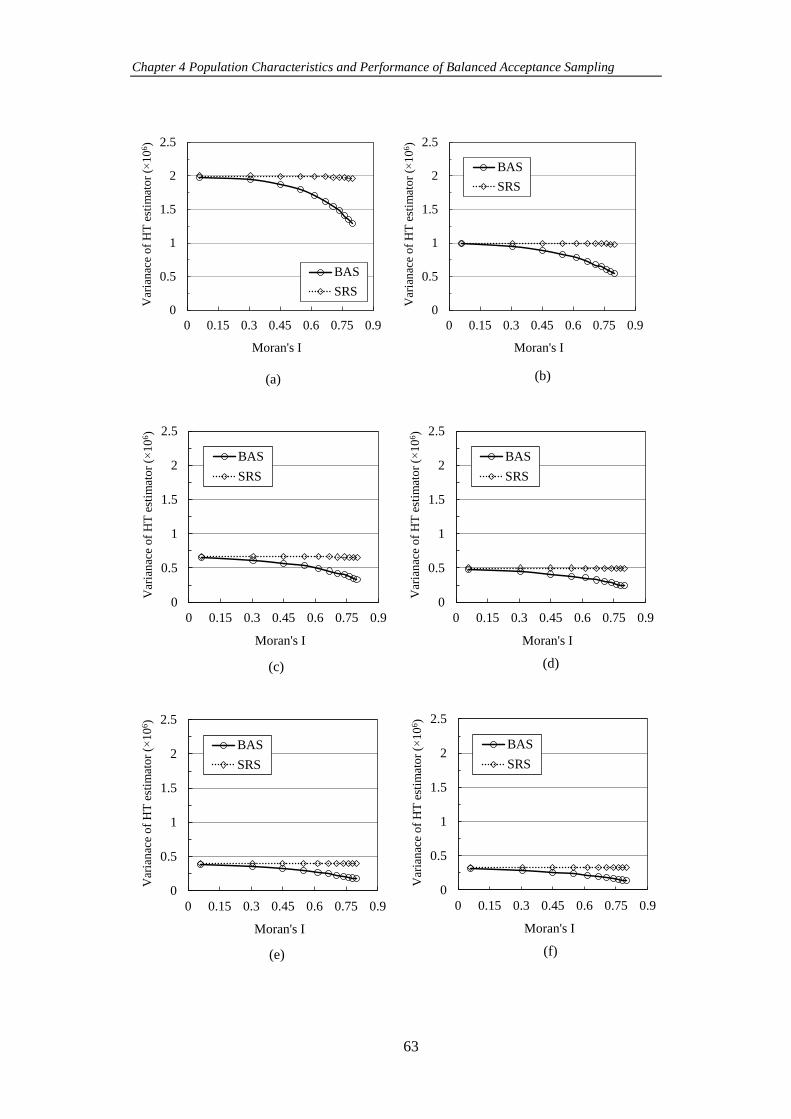
Chapter 4 Population Characteristics and Performance of Balanced Acceptance Sampling
63
(a) (b)
0
0.5
1
1.5
2
2.5
0 0.15 0.3 0.45 0.6 0.75 0.9
Moran's I
BAS
SRS
Var
ian
ace
of
HT
est
imat
or
( 1
06)
0
0.5
1
1.5
2
2.5
0 0.15 0.3 0.45 0.6 0.75 0.9
Moran's I
BAS
SRS
Var
ian
ace
of
HT
est
imat
or
( 1
06)
(c) (d)
0
0.5
1
1.5
2
2.5
0 0.15 0.3 0.45 0.6 0.75 0.9
Moran's I
BAS
SRS
Var
ian
ace
of
HT
est
imat
or
( 1
06)
0
0.5
1
1.5
2
2.5
0 0.15 0.3 0.45 0.6 0.75 0.9
Moran's I
BAS
SRS
Var
ian
ace
of
HT
est
imat
or
( 1
06)
(e) (f)
0
0.5
1
1.5
2
2.5
0 0.15 0.3 0.45 0.6 0.75 0.9
Moran's I
BAS
SRS
Var
ian
ace
of
HT
est
imat
or
( 1
06)
0
0.5
1
1.5
2
2.5
0 0.15 0.3 0.45 0.6 0.75 0.9
Moran's I
BAS
SRS
Var
ian
ace
of
HT
est
imat
or
( 1
06)
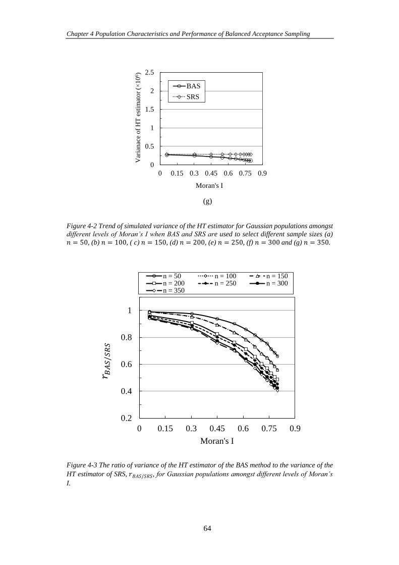
Chapter 4 Population Characteristics and Performance of Balanced Acceptance Sampling
64
Figure 4-2 Trend of simulated variance of the HT estimator for Gaussian populations amongst
different levels of Moran’s I when BAS and SRS are used to select different sample sizes (a)
𝑛 = 50, (b) 𝑛 = 100, ( c) 𝑛 = 150, (d) 𝑛 = 200, (e) 𝑛 = 250, (f) 𝑛 = 300 and (g) 𝑛 = 350.
Figure 4-3 The ratio of variance of the HT estimator of the BAS method to the variance of the
HT estimator of SRS, 𝑟𝐵𝐴𝑆/𝑆𝑅𝑆, for Gaussian populations amongst different levels of Moran’s
I.
(g)
0
0.5
1
1.5
2
2.5
0 0.15 0.3 0.45 0.6 0.75 0.9
Moran's I
BAS
SRS
Var
ian
ace
of
HT
est
imat
or
( 1
06)
0.2
0.4
0.6
0.8
1
0 0.15 0.3 0.45 0.6 0.75 0.9
Moran's I
n = 50 n = 100 n = 150n = 200 n = 250 n = 300n = 350
Chapter 4 Population Characteristics and Performance of Balanced Acceptance Sampling
65
As can be seen in Table 4-1, Figure 4-2 and Figure 4-3, for increasing spatial
autocorrelation, the BAS method is more efficient than SRS for all sample sizes. The
variance of the HT estimator with SRS is almost constant for different levels of Moran’s
I, and there is no relationship between the underlying population’s spatial pattern and
the precision of the estimate. In contrast, there is a significant gap between the
simulated variance of the HT estimator in the population with a low Moran’s I value
and in the population with a high Moran’s I value, when BAS is used for selecting the
samples. This emphasizes how using BAS for a spatially autocorrelated population
with Gaussian response can increase the precision of the estimates.
4.2.2 Using BAS in Populations Where Responses are Binary Data
Populations that can be characterised by a Bernoulli distribution where its units have
binary responses, such as employment status (employed/unemployed). In order to
understand whether the BAS method can be an efficient sampling design to select
samples from this kind of population, a simulation study similar to that performed in
the previous subsection was conducted. The difference here is that instead of using a
normal distribution, the observations were generated from a Bernoulli response
distribution. Using “geoR” package in R (R Core Team, 2017), different spatial
structures of a population with a Bernoulli distribution with parameter 𝑝 = 0.5 from
complete spatial randomness (Moran’s I = 0.006) to spatial clustered (Moran’s I = 0.80)
were generated. Some discussions on generating spatially auto-correlated data can be
found in Appendix A. Considered spatial features of some of the generated Bernoulli
populations with 𝑝 = 0.5 are illustrated in Figure 4-4.
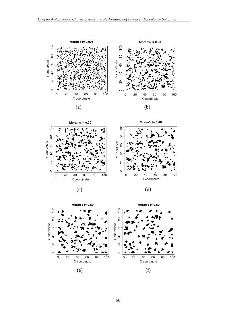
Chapter 4 Population Characteristics and Performance of Balanced Acceptance Sampling
66
(a) (b)
(c) (d)
(e) (f)
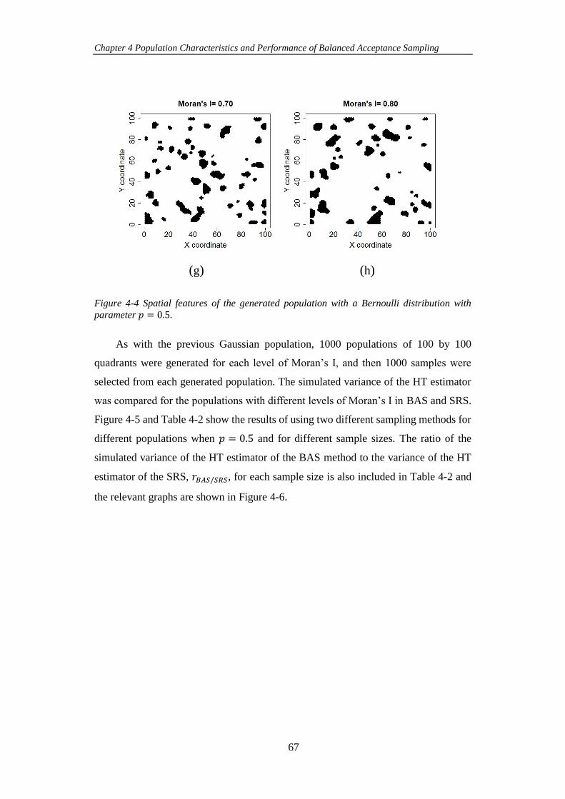
Chapter 4 Population Characteristics and Performance of Balanced Acceptance Sampling
67
Figure 4-4 Spatial features of the generated population with a Bernoulli distribution with
parameter 𝑝 = 0.5.
As with the previous Gaussian population, 1000 populations of 100 by 100
quadrants were generated for each level of Moran’s I, and then 1000 samples were
selected from each generated population. The simulated variance of the HT estimator
was compared for the populations with different levels of Moran’s I in BAS and SRS.
Figure 4-5 and Table 4-2 show the results of using two different sampling methods for
different populations when 𝑝 = 0.5 and for different sample sizes. The ratio of the
simulated variance of the HT estimator of the BAS method to the variance of the HT
estimator of the SRS, 𝑟𝐵𝐴𝑆/𝑆𝑅𝑆, for each sample size is also included in Table 4-2 and
the relevant graphs are shown in Figure 4-6.
(g) (h)
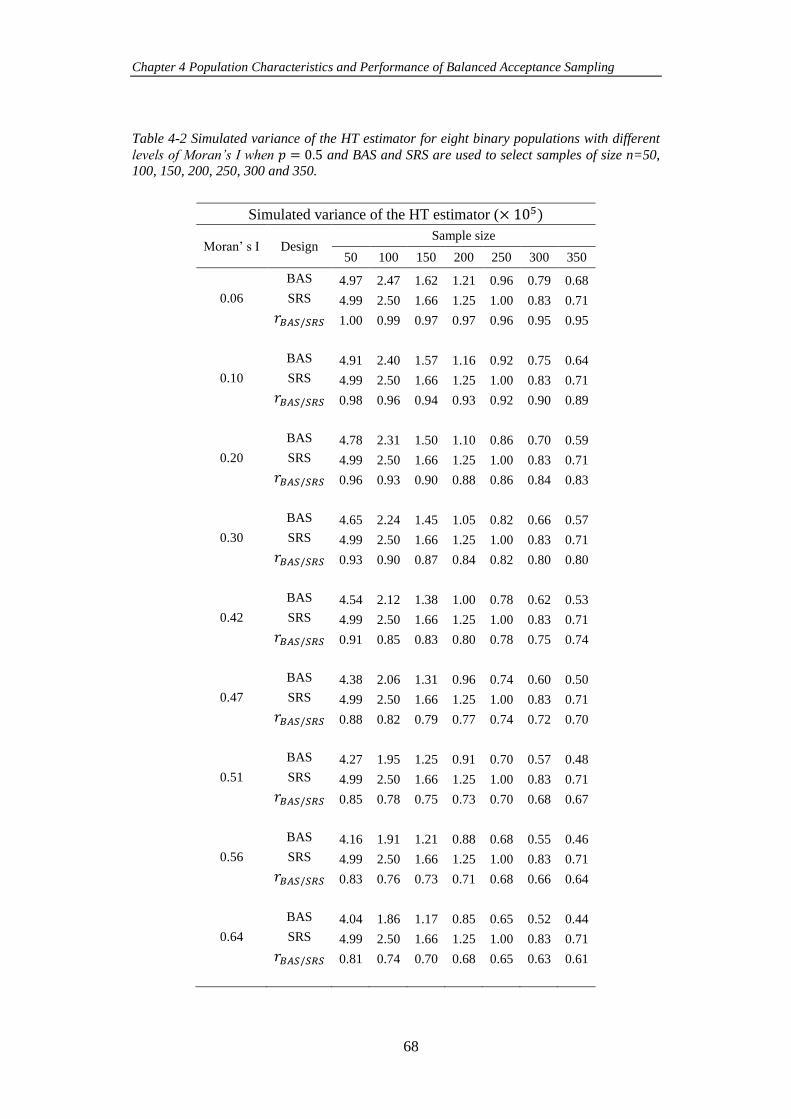
Chapter 4 Population Characteristics and Performance of Balanced Acceptance Sampling
68
Table 4-2 Simulated variance of the HT estimator for eight binary populations with different
levels of Moran’s I when 𝑝 = 0.5 and BAS and SRS are used to select samples of size n=50, 100, 150, 200, 250, 300 and 350.
Simulated variance of the HT estimator (× 105)
Moran’ s I Design Sample size
50 100 150 200 250 300 350
BAS 4.97 2.47 1.62 1.21 0.96 0.79 0.68
0.06 SRS 4.99 2.50 1.66 1.25 1.00 0.83 0.71 𝑟𝐵𝐴𝑆/𝑆𝑅𝑆 1.00 0.99 0.97 0.97 0.96 0.95 0.95
BAS 4.91 2.40 1.57 1.16 0.92 0.75 0.64
0.10 SRS 4.99 2.50 1.66 1.25 1.00 0.83 0.71 𝑟𝐵𝐴𝑆/𝑆𝑅𝑆 0.98 0.96 0.94 0.93 0.92 0.90 0.89
BAS 4.78 2.31 1.50 1.10 0.86 0.70 0.59
0.20 SRS 4.99 2.50 1.66 1.25 1.00 0.83 0.71 𝑟𝐵𝐴𝑆/𝑆𝑅𝑆 0.96 0.93 0.90 0.88 0.86 0.84 0.83
BAS 4.65 2.24 1.45 1.05 0.82 0.66 0.57
0.30 SRS 4.99 2.50 1.66 1.25 1.00 0.83 0.71 𝑟𝐵𝐴𝑆/𝑆𝑅𝑆 0.93 0.90 0.87 0.84 0.82 0.80 0.80
BAS 4.54 2.12 1.38 1.00 0.78 0.62 0.53
0.42 SRS 4.99 2.50 1.66 1.25 1.00 0.83 0.71 𝑟𝐵𝐴𝑆/𝑆𝑅𝑆 0.91 0.85 0.83 0.80 0.78 0.75 0.74
BAS 4.38 2.06 1.31 0.96 0.74 0.60 0.50
0.47 SRS 4.99 2.50 1.66 1.25 1.00 0.83 0.71 𝑟𝐵𝐴𝑆/𝑆𝑅𝑆 0.88 0.82 0.79 0.77 0.74 0.72 0.70
BAS 4.27 1.95 1.25 0.91 0.70 0.57 0.48
0.51 SRS 4.99 2.50 1.66 1.25 1.00 0.83 0.71 𝑟𝐵𝐴𝑆/𝑆𝑅𝑆 0.85 0.78 0.75 0.73 0.70 0.68 0.67
BAS 4.16 1.91 1.21 0.88 0.68 0.55 0.46
0.56 SRS 4.99 2.50 1.66 1.25 1.00 0.83 0.71 𝑟𝐵𝐴𝑆/𝑆𝑅𝑆 0.83 0.76 0.73 0.71 0.68 0.66 0.64
BAS 4.04 1.86 1.17 0.85 0.65 0.52 0.44
0.64 SRS 4.99 2.50 1.66 1.25 1.00 0.83 0.71 𝑟𝐵𝐴𝑆/𝑆𝑅𝑆 0.81 0.74 0.70 0.68 0.65 0.63 0.61
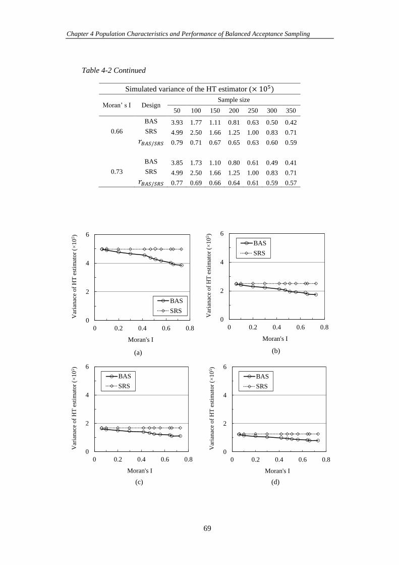
Chapter 4 Population Characteristics and Performance of Balanced Acceptance Sampling
69
Table 4-2 Continued
Simulated variance of the HT estimator (× 105)
Moran’ s I Design Sample size
50 100 150 200 250 300 350
BAS 3.93 1.77 1.11 0.81 0.63 0.50 0.42
0.66 SRS 4.99 2.50 1.66 1.25 1.00 0.83 0.71 𝑟𝐵𝐴𝑆/𝑆𝑅𝑆 0.79 0.71 0.67 0.65 0.63 0.60 0.59
BAS 3.85 1.73 1.10 0.80 0.61 0.49 0.41
0.73 SRS 4.99 2.50 1.66 1.25 1.00 0.83 0.71 𝑟𝐵𝐴𝑆/𝑆𝑅𝑆 0.77 0.69 0.66 0.64 0.61 0.59 0.57
(a) (b)
0
2
4
6
0 0.2 0.4 0.6 0.8
Moran's I
BAS
SRS
Var
ian
ace
of
HT
est
imat
or
( 1
05)
0
2
4
6
0 0.2 0.4 0.6 0.8
Moran's I
BAS
SRS
Var
ian
ace
of
HT
est
imat
or
( 1
05)
0
2
4
6
0 0.2 0.4 0.6 0.8
Moran's I
BAS
SRS
Var
ian
ace
of
HT
est
imat
or
( 1
05)
0
2
4
6
0 0.2 0.4 0.6 0.8
Moran's I
BAS
SRS
Var
ian
ace
of
HT
est
imat
or
( 1
05)
(c) (d)
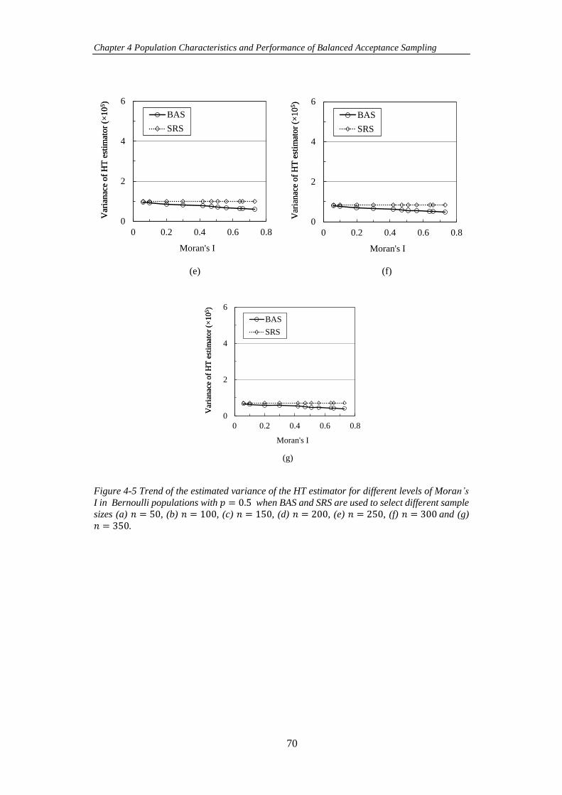
Chapter 4 Population Characteristics and Performance of Balanced Acceptance Sampling
70
Figure 4-5 Trend of the estimated variance of the HT estimator for different levels of Moran’s
I in Bernoulli populations with 𝑝 = 0.5 when BAS and SRS are used to select different sample
sizes (a) 𝑛 = 50, (b) 𝑛 = 100, (c) 𝑛 = 150, (d) 𝑛 = 200, (e) 𝑛 = 250, (f) 𝑛 = 300 and (g)
𝑛 = 350.
0
2
4
6
0 0.2 0.4 0.6 0.8
Moran's I
BAS
SRS
Var
ian
ace
of
HT
est
imat
or
( 1
05)
Var
ian
ace
of
HT
est
imat
or
( 1
05)
0
2
4
6
0 0.2 0.4 0.6 0.8
Moran's I
BAS
SRS
Var
ian
ace
of
HT
est
imat
or
( 1
05)
Var
ian
ace
of
HT
est
imat
or
( 1
05)
(e) (f)
0
2
4
6
0 0.2 0.4 0.6 0.8
Moran's I
BAS
SRS
Var
ian
ace
of
HT
est
imat
or
( 1
05)
Var
ian
ace
of
HT
est
imat
or
( 1
05)
(g)
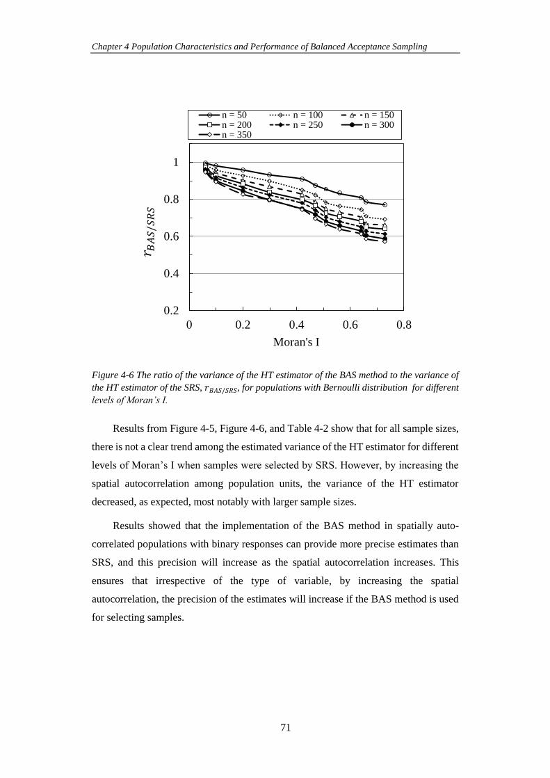
Chapter 4 Population Characteristics and Performance of Balanced Acceptance Sampling
71
Figure 4-6 The ratio of the variance of the HT estimator of the BAS method to the variance of
the HT estimator of the SRS, 𝑟𝐵𝐴𝑆/𝑆𝑅𝑆, for populations with Bernoulli distribution for different
levels of Moran’s I.
Results from Figure 4-5, Figure 4-6, and Table 4-2 show that for all sample sizes,
there is not a clear trend among the estimated variance of the HT estimator for different
levels of Moran’s I when samples were selected by SRS. However, by increasing the
spatial autocorrelation among population units, the variance of the HT estimator
decreased, as expected, most notably with larger sample sizes.
Results showed that the implementation of the BAS method in spatially auto-
correlated populations with binary responses can provide more precise estimates than
SRS, and this precision will increase as the spatial autocorrelation increases. This
ensures that irrespective of the type of variable, by increasing the spatial
autocorrelation, the precision of the estimates will increase if the BAS method is used
for selecting samples.
0.2
0.4
0.6
0.8
1
0 0.2 0.4 0.6 0.8
Moran's I
n = 50 n = 100 n = 150n = 200 n = 250 n = 300n = 350
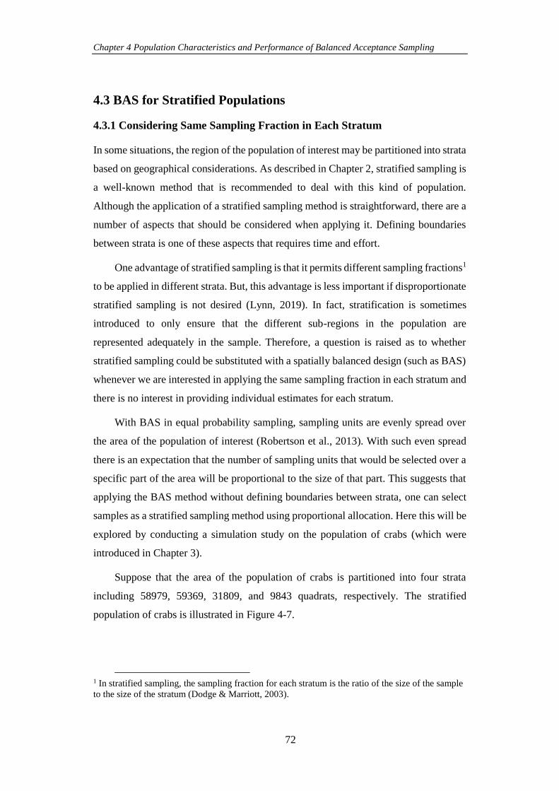
Chapter 4 Population Characteristics and Performance of Balanced Acceptance Sampling
72
4.3 BAS for Stratified Populations
4.3.1 Considering Same Sampling Fraction in Each Stratum
In some situations, the region of the population of interest may be partitioned into strata
based on geographical considerations. As described in Chapter 2, stratified sampling is
a well-known method that is recommended to deal with this kind of population.
Although the application of a stratified sampling method is straightforward, there are a
number of aspects that should be considered when applying it. Defining boundaries
between strata is one of these aspects that requires time and effort.
One advantage of stratified sampling is that it permits different sampling fractions1
to be applied in different strata. But, this advantage is less important if disproportionate
stratified sampling is not desired (Lynn, 2019). In fact, stratification is sometimes
introduced to only ensure that the different sub-regions in the population are
represented adequately in the sample. Therefore, a question is raised as to whether
stratified sampling could be substituted with a spatially balanced design (such as BAS)
whenever we are interested in applying the same sampling fraction in each stratum and
there is no interest in providing individual estimates for each stratum.
With BAS in equal probability sampling, sampling units are evenly spread over
the area of the population of interest (Robertson et al., 2013). With such even spread
there is an expectation that the number of sampling units that would be selected over a
specific part of the area will be proportional to the size of that part. This suggests that
applying the BAS method without defining boundaries between strata, one can select
samples as a stratified sampling method using proportional allocation. Here this will be
explored by conducting a simulation study on the population of crabs (which were
introduced in Chapter 3).
Suppose that the area of the population of crabs is partitioned into four strata
including 58979, 59369, 31809, and 9843 quadrats, respectively. The stratified
population of crabs is illustrated in Figure 4-7.
1 In stratified sampling, the sampling fraction for each stratum is the ratio of the size of the sample
to the size of the stratum (Dodge & Marriott, 2003).
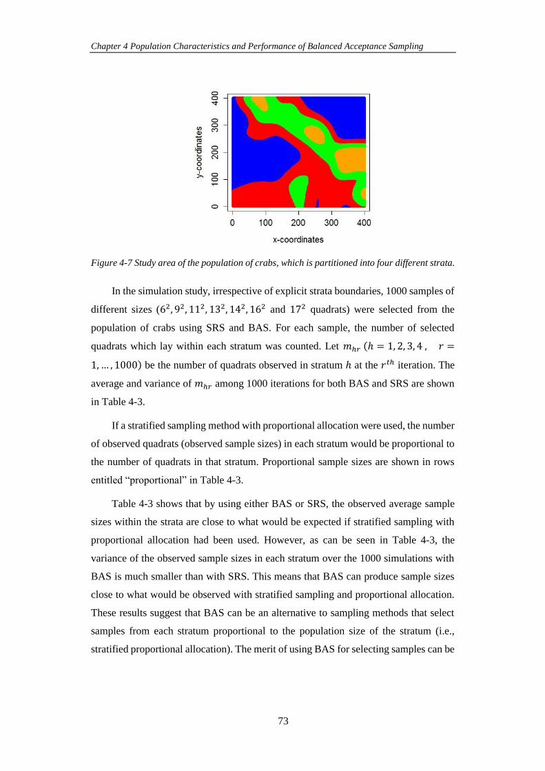
Chapter 4 Population Characteristics and Performance of Balanced Acceptance Sampling
73
Figure 4-7 Study area of the population of crabs, which is partitioned into four different strata.
In the simulation study, irrespective of explicit strata boundaries, 1000 samples of
different sizes (62, 92, 112, 132, 142, 162 and 172 quadrats) were selected from the
population of crabs using SRS and BAS. For each sample, the number of selected
quadrats which lay within each stratum was counted. Let 𝑚ℎ𝑟 (ℎ = 1, 2, 3, 4 , 𝑟 =
1, … , 1000) be the number of quadrats observed in stratum ℎ at the 𝑟𝑡ℎ iteration. The
average and variance of 𝑚ℎ𝑟 among 1000 iterations for both BAS and SRS are shown
in Table 4-3.
If a stratified sampling method with proportional allocation were used, the number
of observed quadrats (observed sample sizes) in each stratum would be proportional to
the number of quadrats in that stratum. Proportional sample sizes are shown in rows
entitled “proportional” in Table 4-3.
Table 4-3 shows that by using either BAS or SRS, the observed average sample
sizes within the strata are close to what would be expected if stratified sampling with
proportional allocation had been used. However, as can be seen in Table 4-3, the
variance of the observed sample sizes in each stratum over the 1000 simulations with
BAS is much smaller than with SRS. This means that BAS can produce sample sizes
close to what would be observed with stratified sampling and proportional allocation.
These results suggest that BAS can be an alternative to sampling methods that select
samples from each stratum proportional to the population size of the stratum (i.e.,
stratified proportional allocation). The merit of using BAS for selecting samples can be
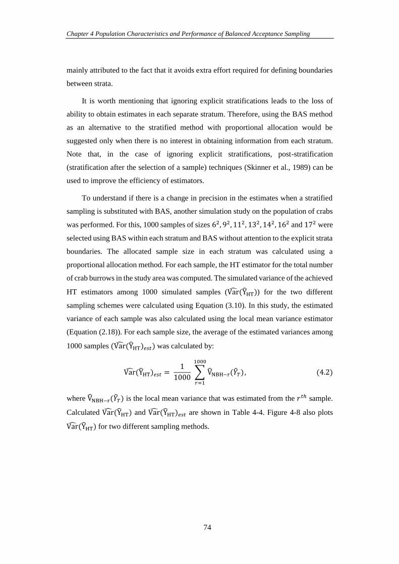
Chapter 4 Population Characteristics and Performance of Balanced Acceptance Sampling
74
mainly attributed to the fact that it avoids extra effort required for defining boundaries
between strata.
It is worth mentioning that ignoring explicit stratifications leads to the loss of
ability to obtain estimates in each separate stratum. Therefore, using the BAS method
as an alternative to the stratified method with proportional allocation would be
suggested only when there is no interest in obtaining information from each stratum.
Note that, in the case of ignoring explicit stratifications, post-stratification
(stratification after the selection of a sample) techniques (Skinner et al., 1989) can be
used to improve the efficiency of estimators.
To understand if there is a change in precision in the estimates when a stratified
sampling is substituted with BAS, another simulation study on the population of crabs
was performed. For this, 1000 samples of sizes 62, 92, 112, 132, 142, 162 and 172 were
selected using BAS within each stratum and BAS without attention to the explicit strata
boundaries. The allocated sample size in each stratum was calculated using a
proportional allocation method. For each sample, the HT estimator for the total number
of crab burrows in the study area was computed. The simulated variance of the achieved
HT estimators among 1000 simulated samples (Var(YHT)) for the two different
sampling schemes were calculated using Equation (3.10). In this study, the estimated
variance of each sample was also calculated using the local mean variance estimator
(Equation (2.18)). For each sample size, the average of the estimated variances among
1000 samples (Var(YHT)𝑒𝑠𝑡) was calculated by:
Var(YHT)𝑒𝑠𝑡 = 1
1000 ∑ VNBH−r(��𝑇)
1000
𝑟=1
, (4.2)
where VNBH−r(��𝑇) is the local mean variance that was estimated from the 𝑟𝑡ℎ sample.
Calculated Var(YHT) and Var(YHT)𝑒𝑠𝑡 are shown in Table 4-4. Figure 4-8 also plots
Var(YHT) for two different sampling methods.
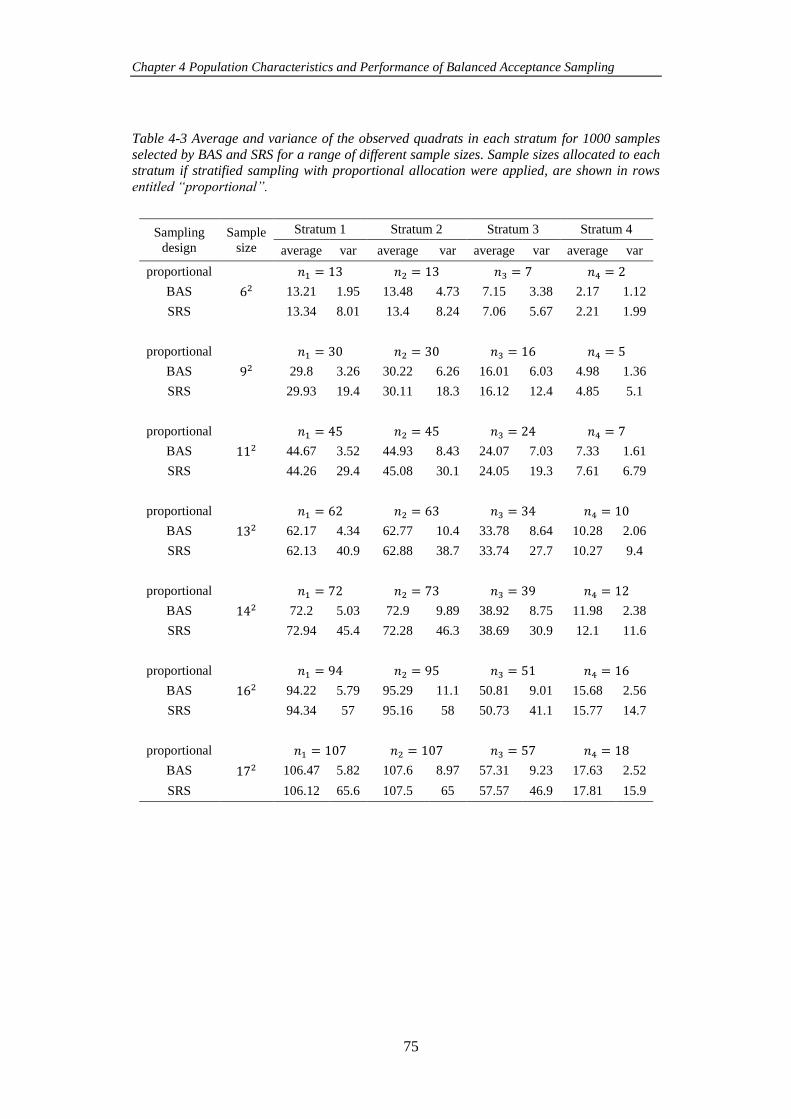
Chapter 4 Population Characteristics and Performance of Balanced Acceptance Sampling
75
Table 4-3 Average and variance of the observed quadrats in each stratum for 1000 samples
selected by BAS and SRS for a range of different sample sizes. Sample sizes allocated to each stratum if stratified sampling with proportional allocation were applied, are shown in rows
entitled “proportional”.
Sampling
design
Sample
size
Stratum 1 Stratum 2 Stratum 3 Stratum 4
average var average var average var average var
proportional
62
𝑛1 = 13 𝑛2 = 13 𝑛3 = 7 𝑛4 = 2
BAS 13.21 1.95 13.48 4.73 7.15 3.38 2.17 1.12
SRS 13.34 8.01 13.4 8.24 7.06 5.67 2.21 1.99
proportional
92
𝑛1 = 30 𝑛2 = 30 𝑛3 = 16 𝑛4 = 5
BAS 29.8 3.26 30.22 6.26 16.01 6.03 4.98 1.36
SRS 29.93 19.4 30.11 18.3 16.12 12.4 4.85 5.1
proportional
112
𝑛1 = 45 𝑛2 = 45 𝑛3 = 24 𝑛4 = 7
BAS 44.67 3.52 44.93 8.43 24.07 7.03 7.33 1.61
SRS 44.26 29.4 45.08 30.1 24.05 19.3 7.61 6.79
proportional
132
𝑛1 = 62 𝑛2 = 63 𝑛3 = 34 𝑛4 = 10
BAS 62.17 4.34 62.77 10.4 33.78 8.64 10.28 2.06
SRS 62.13 40.9 62.88 38.7 33.74 27.7 10.27 9.4
proportional
142
𝑛1 = 72 𝑛2 = 73 𝑛3 = 39 𝑛4 = 12
BAS 72.2 5.03 72.9 9.89 38.92 8.75 11.98 2.38
SRS 72.94 45.4 72.28 46.3 38.69 30.9 12.1 11.6
proportional
162
𝑛1 = 94 𝑛2 = 95 𝑛3 = 51 𝑛4 = 16
BAS 94.22 5.79 95.29 11.1 50.81 9.01 15.68 2.56
SRS 94.34 57 95.16 58 50.73 41.1 15.77 14.7
proportional
172
𝑛1 = 107 𝑛2 = 107 𝑛3 = 57 𝑛4 = 18
BAS 106.47 5.82 107.6 8.97 57.31 9.23 17.63 2.52
SRS 106.12 65.6 107.5 65 57.57 46.9 17.81 15.9
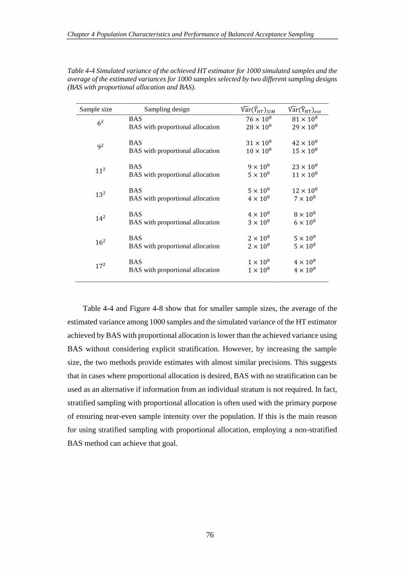
Chapter 4 Population Characteristics and Performance of Balanced Acceptance Sampling
76
Table 4-4 Simulated variance of the achieved HT estimator for 1000 simulated samples and the
average of the estimated variances for 1000 samples selected by two different sampling designs (BAS with proportional allocation and BAS).
Sample size Sampling design Var(��𝐻𝑇)𝑆𝐼𝑀 Var(YHT)𝑒𝑠𝑡
62 BAS 76 × 108 81 × 108 BAS with proportional allocation 28 × 108 29 × 108
92 BAS 31 × 108 42 × 108 BAS with proportional allocation 10 × 108 15 × 108
112 BAS 9 × 10⁸ 23 × 108 BAS with proportional allocation 5 × 10⁸ 11 × 108
132 BAS 5 × 10⁸ 12 × 108 BAS with proportional allocation 4 × 10⁸ 7 × 10⁸
142 BAS 4 × 10⁸ 8 × 10⁸ BAS with proportional allocation 3 × 10⁸ 6 × 10⁸
162 BAS 2 × 10⁸ 5 × 10⁸ BAS with proportional allocation 2 × 10⁸ 5 × 10⁸
172 BAS 1 × 10⁸ 4 × 10⁸ BAS with proportional allocation 1 × 10⁸ 4 × 10⁸
Table 4-4 and Figure 4-8 show that for smaller sample sizes, the average of the
estimated variance among 1000 samples and the simulated variance of the HT estimator
achieved by BAS with proportional allocation is lower than the achieved variance using
BAS without considering explicit stratification. However, by increasing the sample
size, the two methods provide estimates with almost similar precisions. This suggests
that in cases where proportional allocation is desired, BAS with no stratification can be
used as an alternative if information from an individual stratum is not required. In fact,
stratified sampling with proportional allocation is often used with the primary purpose
of ensuring near-even sample intensity over the population. If this is the main reason
for using stratified sampling with proportional allocation, employing a non-stratified
BAS method can achieve that goal.
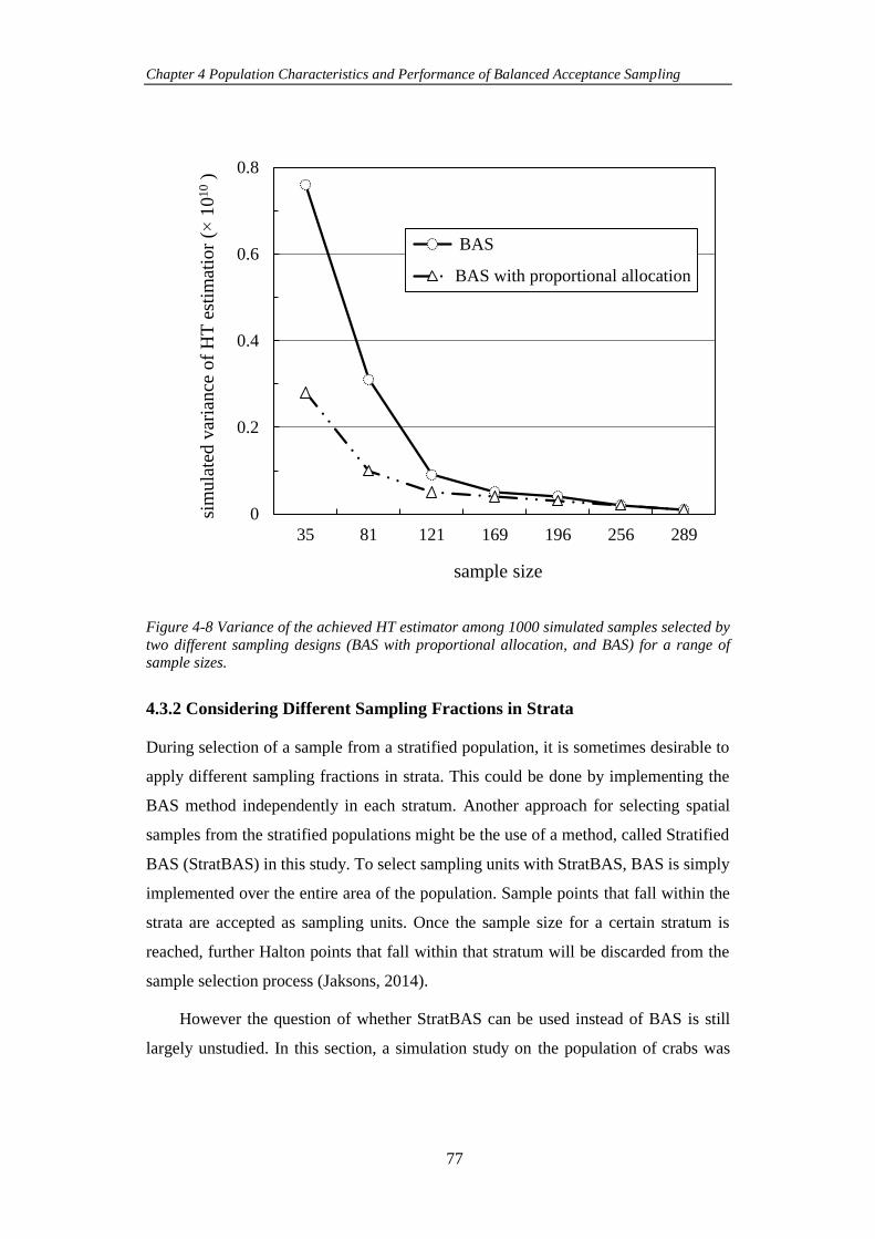
Chapter 4 Population Characteristics and Performance of Balanced Acceptance Sampling
77
Figure 4-8 Variance of the achieved HT estimator among 1000 simulated samples selected by
two different sampling designs (BAS with proportional allocation, and BAS) for a range of sample sizes.
4.3.2 Considering Different Sampling Fractions in Strata
During selection of a sample from a stratified population, it is sometimes desirable to
apply different sampling fractions in strata. This could be done by implementing the
BAS method independently in each stratum. Another approach for selecting spatial
samples from the stratified populations might be the use of a method, called Stratified
BAS (StratBAS) in this study. To select sampling units with StratBAS, BAS is simply
implemented over the entire area of the population. Sample points that fall within the
strata are accepted as sampling units. Once the sample size for a certain stratum is
reached, further Halton points that fall within that stratum will be discarded from the
sample selection process (Jaksons, 2014).
However the question of whether StratBAS can be used instead of BAS is still
largely unstudied. In this section, a simulation study on the population of crabs was
0
0.2
0.4
0.6
0.8
35 81 121 169 196 256 289
sim
ula
ted
var
ian
ce o
f H
T e
stim
atio
r (
10
10
)
sample size
BAS
BAS with proportional allocation
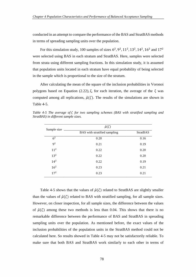
Chapter 4 Population Characteristics and Performance of Balanced Acceptance Sampling
78
conducted in an attempt to compare the performance of the BAS and StratBAS methods
in terms of spreading sampling units over the population.
For this simulation study, 100 samples of sizes 62, 92, 112, 132, 142, 162 and 172
were selected using BAS in each stratum and StratBAS. Here, samples were selected
from strata using different sampling fractions. In this simulation study, it is assumed
that population units located in each stratum have equal probability of being selected
in the sample which is proportional to the size of the stratum.
After calculating the mean of the square of the inclusion probabilities in Voronoi
polygons based on Equation (2.22), ζ, for each iteration, the average of the ζ was
computed among all replications, ��(𝜁). The results of the simulations are shown in
Table 4-5.
Table 4-5 The average of 𝜁 for two sampling schemes (BAS with stratified sampling and
StratBAS) in different sample sizes.
Sample size ��(𝜁)
BAS with stratified sampling StratBAS
62 0.20 0.16
92 0.21 0.19
112 0.22 0.20
132 0.22 0.20
142 0.22 0.19
162 0.23 0.21
172 0.23 0.21
Table 4-5 shows that the values of ��(𝜁) related to StratBAS are slightly smaller
than the values of ��(𝜁) related to BAS with stratified sampling, for all sample sizes.
However, on closer inspection, for all sample sizes, the difference between the values
of ��(𝜁) among these two methods is less than 0.04. This shows that there is no
remarkable difference between the performance of BAS and StratBAS in spreading
sampling units over the population. As mentioned before, the exact values of the
inclusion probabilities of the population units in the StratBAS method could not be
calculated here. So results showed in Table 4-5 may not be satisfactorily reliable. To
make sure that both BAS and StratBAS work similarly to each other in terms of
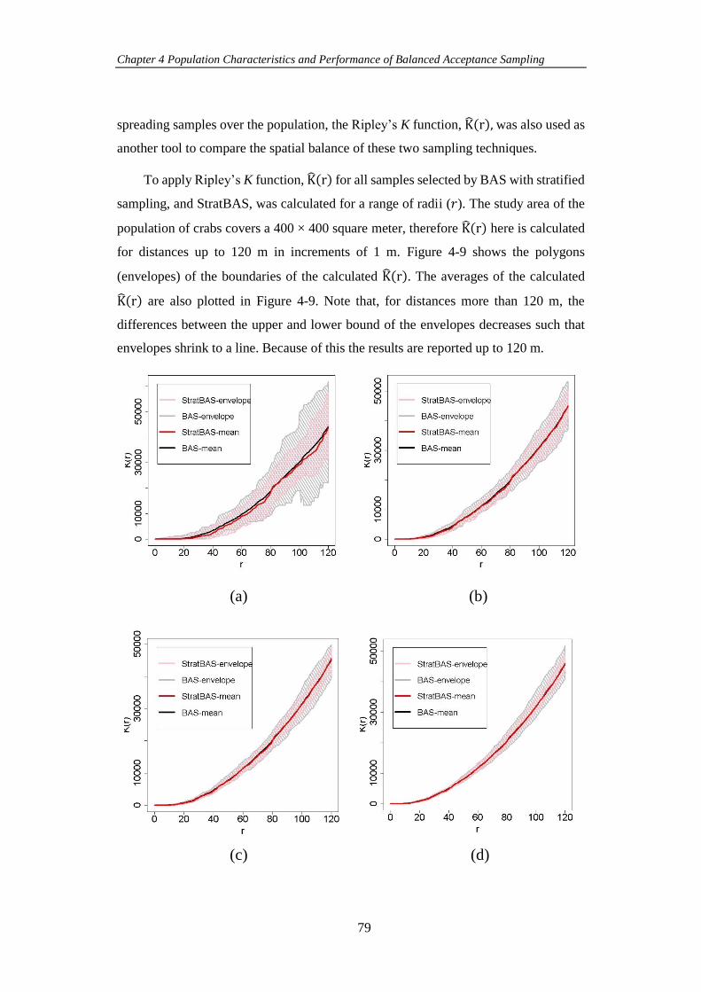
Chapter 4 Population Characteristics and Performance of Balanced Acceptance Sampling
79
spreading samples over the population, the Ripley’s K function, K(r), was also used as
another tool to compare the spatial balance of these two sampling techniques.
To apply Ripley’s K function, K(r) for all samples selected by BAS with stratified
sampling, and StratBAS, was calculated for a range of radii (𝑟). The study area of the
population of crabs covers a 400 × 400 square meter, therefore K(r) here is calculated
for distances up to 120 m in increments of 1 m. Figure 4-9 shows the polygons
(envelopes) of the boundaries of the calculated K(r). The averages of the calculated
K(r) are also plotted in Figure 4-9. Note that, for distances more than 120 m, the
differences between the upper and lower bound of the envelopes decreases such that
envelopes shrink to a line. Because of this the results are reported up to 120 m.
(a) (b)
(c) (d)
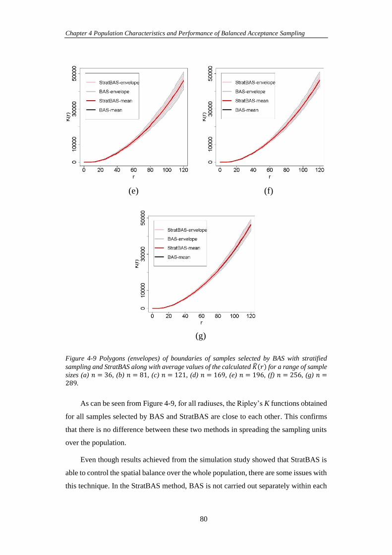
Chapter 4 Population Characteristics and Performance of Balanced Acceptance Sampling
80
Figure 4-9 Polygons (envelopes) of boundaries of samples selected by BAS with stratified
sampling and StratBAS along with average values of the calculated ��(𝑟) for a range of sample
sizes (a) 𝑛 = 36, (b) 𝑛 = 81, (c) 𝑛 = 121, (d) 𝑛 = 169, (e) 𝑛 = 196, (f) 𝑛 = 256, (g) 𝑛 =289.
As can be seen from Figure 4-9, for all radiuses, the Ripley’s K functions obtained
for all samples selected by BAS and StratBAS are close to each other. This confirms
that there is no difference between these two methods in spreading the sampling units
over the population.
Even though results achieved from the simulation study showed that StratBAS is
able to control the spatial balance over the whole population, there are some issues with
this technique. In the StratBAS method, BAS is not carried out separately within each
(e) (f)
(g)
Chapter 4 Population Characteristics and Performance of Balanced Acceptance Sampling
81
stratum, causing the sampling selection process in each stratum to be dependent on
other strata. Hence, the inclusion probabilities of the population units are difficult to
compute. In addition, the formulas used in the common stratified sampling method may
not be applicable for estimating the parameters of interest with StratBAS. This may
lead to an estimation of the parameters with a bigger variance.
Hence, considering the advantages of the BAS method where it is applied within
each stratum, over the StratBAS method, the use of BAS within each stratum
independently is recommended instead of StratBAS.
4.4 Conclusions
This chapter evaluated the effect of spatial autocorrelation of observations on the
precision of the population estimates when BAS is used to select the sample. To test
this, two simulation studies were conducted on two different types of populations
(populations where responses have Gaussian and Bernoulli distribution). The results of
the simulation studies showed that in both populations, by increasing the spatial
autocorrelation (which is measured by Moran’s I in this thesis), the precision of the
population estimates increased compared to selecting the sample by SRS.
This chapter also investigated the application of BAS in stratified populations. For
this, simulation studies were performed on a population derived from a study of counts
of crab burrows. The simulation studies showed that BAS can be considered as an
alternative method for stratified sampling when proportional allocation is designed. In
fact, when BAS is used as an alternative to proportional allocation in stratified
sampling, it has the advantage that there is no need to create explicit strata.
In situations that need to use different sampling fractions in strata, samples can be
selected either by applying BAS in each stratum independently or implementing a
technique called StratBAS. This chapter through conducting a simulation study showed
that BAS and StratBAS methods have similar performances in terms of spreading
sampling units over the population.
In this chapter it was found that the BAS method has a number of advantages when
it is used in practical settings in environmental studies. This indicates that the BAS
method has promising potential to be extended to other surveys (i.e., household
Chapter 4 Population Characteristics and Performance of Balanced Acceptance Sampling
82
sampling surveys). In the following chapters, I will investigate this matter by trying to
apply the BAS method and other spatially balanced sampling methods in selecting
sampling units in social studies.
4.5 References
Cochran, W. G. (1977). Sampling Techniques: 3d Ed: Wiley.
Dodge, Y., & Marriott, F. (2003). International Statistical Institute. The Oxford dictionary
of statistical terms.
Grafström, A., Lundström, N. L., & Schelin, L. (2012). Spatially balanced sampling
through the pivotal method. Biometrics, 68(2), 514-520.
Horvitz, D. G., & Thompson, D. J. (1952). A generalization of sampling without
replacement from a finite universe. Journal of the American statistical Association,
47(260), 663-685.
Jaksons, P. (2014). A new approach to adaptive monitoring. (PhD), School of Mathematics
and Statistics, University of Canterbury.
Lynn, P. (2019). The advantage and disadvantage of implicitly stratified sampling. MDA:
methods, data, analyses, 13(2), 14.
R Core Team. (2017). R: A language and environment for statistical computing. R
Foundation for Statistical Computing, Vienna, Austria. URL https://www. R-
project. org.
Robertson, B., Brown, J., McDonald, T., & Jaksons, P. (2013). BAS: balanced acceptance
sampling of natural resources. Biometrics, 69(3), 776-784.
Skinner, C. J., Holt, D., & Smith, T. F. (1989). Analysis of complex surveys: John Wiley &
Sons.
Stevens, D., & Olsen, A. (2004). Spatially balanced sampling of natural resources. Journal
of the American statistical Association, 99(465), 262-278.
83
Spatially Balanced Sampling Methods for
Household Surveys
5.1 Introduction
Household surveying is inherently a spatial science because it almost always involves human
populations living in specific geographic regions. Viewed in this way, the human and physical
characteristics of locations where people live and the interrelationships among neighbouring
people should be considered when designing a sampling survey. Several studies in the
literature have reported that people with similar socio-economic characteristics (for example,
income, occupation, education) tend to live close to each other. For instance, a study
conducted by Kalogirou and Hatzichristos (2007) on modelling the income estimation in
Athens in 2001 showed that there was a very strong relationship between the mean household
income in each area and the proportion of its residents with high levels of education. In
addition, the study indicated that relationship between income and education was not
stationary across the areas of Athens, and the data were spatially autocorrelated. In another
study, Cuberes and Roberts (2015) found that there was a positive correlation between a
household’s income and the distance from their home to the city centre in Britain. In two
separate studies, Kantar and Aktaş (2016) and Alves (2012) also investigated the pattern of
unemployment rate over the provinces in Turkey and subsections of Porto city in Portugal,
respectively. The results of both studies showed that there was a spatial dependency between
neighbouring regions in terms of unemployment rate.
The fact that there is often a spatial similarity between neighbouring people, households
or regions means that selecting nearby sampling units (i.e., people, households, regions) can
provide us with similar information. In household surveys, these samples (that contain nearby
units) are considered as undesirable samples and should be avoided as much as possible in
sample selection.
In the previous chapters, spatially balanced sampling methods were introduced as
sampling methods that avoid selecting nearby units. Although these methods have been
widely used in environmental surveys, they have not been applied in sampling of human
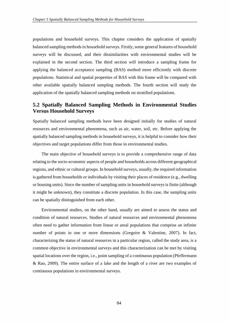
Chapter 5 Spatially Balanced Sampling Methods for Household Surveys
84
populations and household surveys. This chapter considers the application of spatially
balanced sampling methods in household surveys. Firstly, some general features of household
surveys will be discussed, and their dissimilarities with environmental studies will be
explained in the second section. The third section will introduce a sampling frame for
applying the balanced acceptance sampling (BAS) method more efficiently with discrete
populations. Statistical and spatial properties of BAS with this frame will be compared with
other available spatially balanced sampling methods. The fourth section will study the
application of the spatially balanced sampling methods on stratified populations.
5.2 Spatially Balanced Sampling Methods in Environmental Studies
Versus Household Surveys
Spatially balanced sampling methods have been designed initially for studies of natural
resources and environmental phenomena, such as air, water, soil, etc. Before applying the
spatially balanced sampling methods in household surveys, it is helpful to consider how their
objectives and target populations differ from those in environmental studies.
The main objective of household surveys is to provide a comprehensive range of data
relating to the socio-economic aspects of people and households across different geographical
regions, and ethnic or cultural groups. In household surveys, usually, the required information
is gathered from households or individuals by visiting their places of residence (e.g., dwelling
or housing units). Since the number of sampling units in household surveys is finite (although
it might be unknown), they constitute a discrete population. In this case, the sampling units
can be spatially distinguished from each other.
Environmental studies, on the other hand, usually are aimed to assess the status and
condition of natural resources. Studies of natural resources and environmental phenomena
often need to gather information from linear or areal populations that comprise an infinite
number of points in one or more dimensions (Gregoire & Valentine, 2007). In fact,
characterizing the status of natural resources in a particular region, called the study area, is a
common objective in environmental surveys and this characterization can be met by visiting
spatial locations over the region, i.e., point sampling of a continuous population (Pfeffermann
& Rao, 2009). The entire surface of a lake and the length of a river are two examples of
continuous populations in environmental surveys.
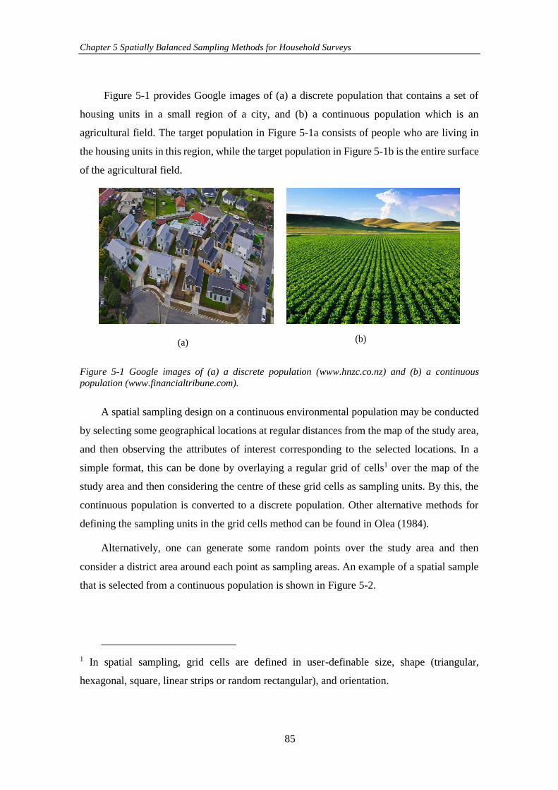
Chapter 5 Spatially Balanced Sampling Methods for Household Surveys
85
Figure 5-1 provides Google images of (a) a discrete population that contains a set of
housing units in a small region of a city, and (b) a continuous population which is an
agricultural field. The target population in Figure 5-1a consists of people who are living in
the housing units in this region, while the target population in Figure 5-1b is the entire surface
of the agricultural field.
Figure 5-1 Google images of (a) a discrete population (www.hnzc.co.nz) and (b) a continuous
population (www.financialtribune.com).
A spatial sampling design on a continuous environmental population may be conducted
by selecting some geographical locations at regular distances from the map of the study area,
and then observing the attributes of interest corresponding to the selected locations. In a
simple format, this can be done by overlaying a regular grid of cells1 over the map of the
study area and then considering the centre of these grid cells as sampling units. By this, the
continuous population is converted to a discrete population. Other alternative methods for
defining the sampling units in the grid cells method can be found in Olea (1984).
Alternatively, one can generate some random points over the study area and then
consider a district area around each point as sampling areas. An example of a spatial sample
that is selected from a continuous population is shown in Figure 5-2.
1 In spatial sampling, grid cells are defined in user-definable size, shape (triangular,
hexagonal, square, linear strips or random rectangular), and orientation.
(a) (b)
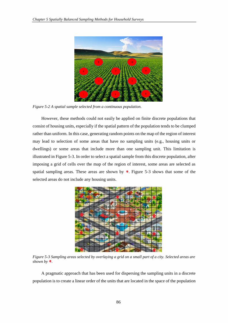
Chapter 5 Spatially Balanced Sampling Methods for Household Surveys
86
Figure 5-2 A spatial sample selected from a continuous population.
However, these methods could not easily be applied on finite discrete populations that
consist of housing units, especially if the spatial pattern of the population tends to be clumped
rather than uniform. In this case, generating random points on the map of the region of interest
may lead to selection of some areas that have no sampling units (e.g., housing units or
dwellings) or some areas that include more than one sampling unit. This limitation is
illustrated in Figure 5-3. In order to select a spatial sample from this discrete population, after
imposing a grid of cells over the map of the region of interest, some areas are selected as
spatial sampling areas. These areas are shown by . Figure 5-3 shows that some of the
selected areas do not include any housing units.
Figure 5-3 Sampling areas selected by overlaying a grid on a small part of a city. Selected areas are
shown by .
A pragmatic approach that has been used for dispersing the sampling units in a discrete
population is to create a linear order of the units that are located in the space of the population
1 2 3
4 5
6 7 8
9 10
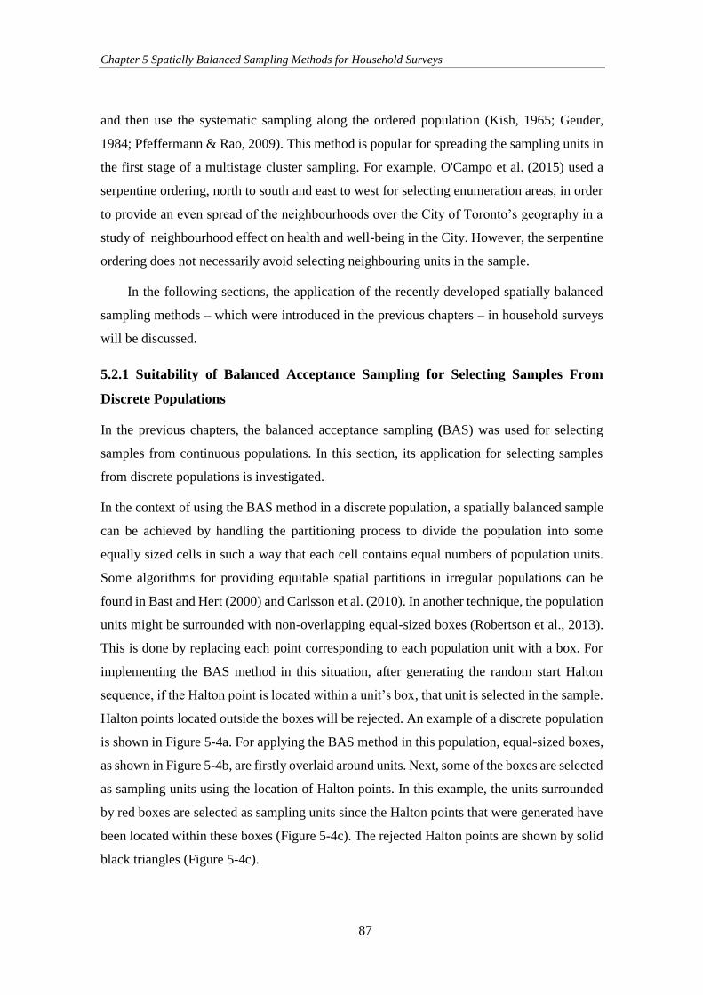
Chapter 5 Spatially Balanced Sampling Methods for Household Surveys
87
and then use the systematic sampling along the ordered population (Kish, 1965; Geuder,
1984; Pfeffermann & Rao, 2009). This method is popular for spreading the sampling units in
the first stage of a multistage cluster sampling. For example, O'Campo et al. (2015) used a
serpentine ordering, north to south and east to west for selecting enumeration areas, in order
to provide an even spread of the neighbourhoods over the City of Toronto’s geography in a
study of neighbourhood effect on health and well-being in the City. However, the serpentine
ordering does not necessarily avoid selecting neighbouring units in the sample.
In the following sections, the application of the recently developed spatially balanced
sampling methods – which were introduced in the previous chapters – in household surveys
will be discussed.
5.2.1 Suitability of Balanced Acceptance Sampling for Selecting Samples From
Discrete Populations
In the previous chapters, the balanced acceptance sampling (BAS) was used for selecting
samples from continuous populations. In this section, its application for selecting samples
from discrete populations is investigated.
In the context of using the BAS method in a discrete population, a spatially balanced sample
can be achieved by handling the partitioning process to divide the population into some
equally sized cells in such a way that each cell contains equal numbers of population units.
Some algorithms for providing equitable spatial partitions in irregular populations can be
found in Bast and Hert (2000) and Carlsson et al. (2010). In another technique, the population
units might be surrounded with non-overlapping equal-sized boxes (Robertson et al., 2013).
This is done by replacing each point corresponding to each population unit with a box. For
implementing the BAS method in this situation, after generating the random start Halton
sequence, if the Halton point is located within a unit’s box, that unit is selected in the sample.
Halton points located outside the boxes will be rejected. An example of a discrete population
is shown in Figure 5-4a. For applying the BAS method in this population, equal-sized boxes,
as shown in Figure 5-4b, are firstly overlaid around units. Next, some of the boxes are selected
as sampling units using the location of Halton points. In this example, the units surrounded
by red boxes are selected as sampling units since the Halton points that were generated have
been located within these boxes (Figure 5-4c). The rejected Halton points are shown by solid
black triangles (Figure 5-4c).
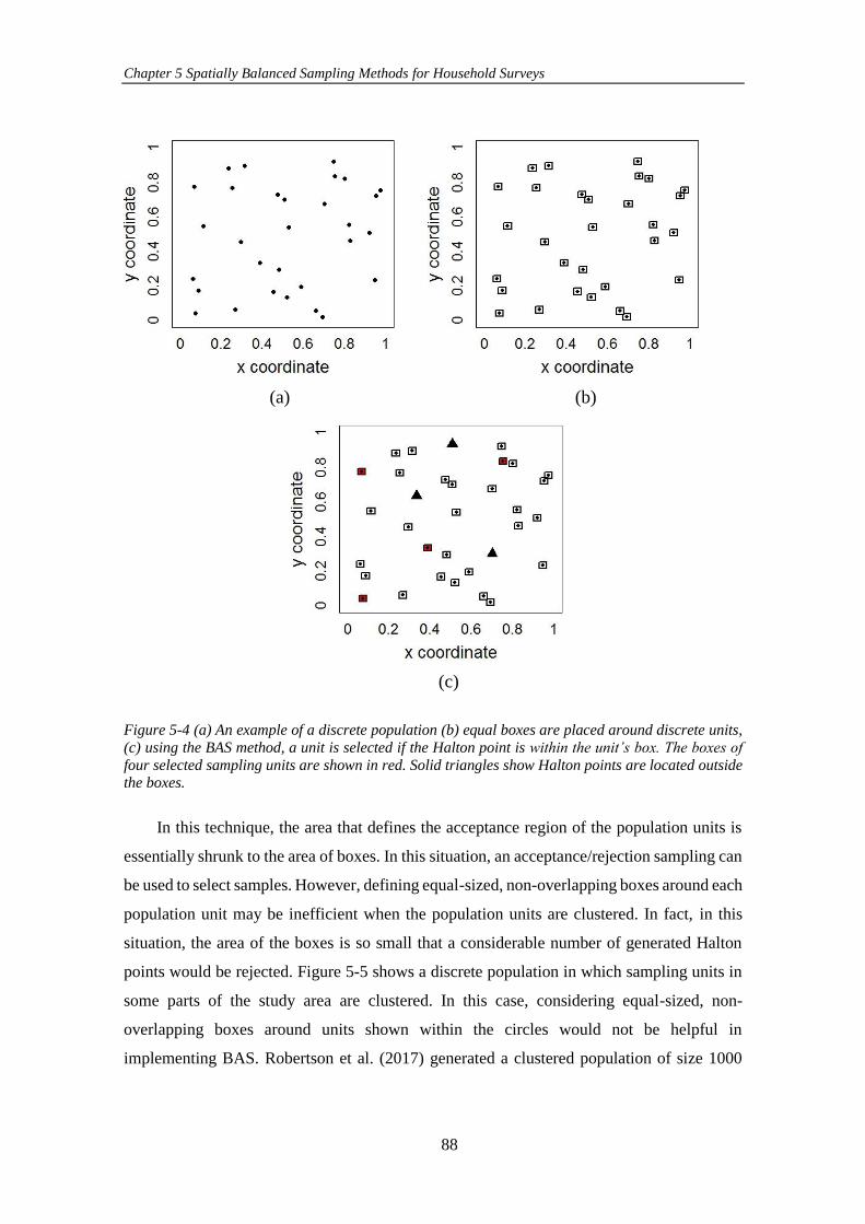
Chapter 5 Spatially Balanced Sampling Methods for Household Surveys
88
Figure 5-4 (a) An example of a discrete population (b) equal boxes are placed around discrete units,
(c) using the BAS method, a unit is selected if the Halton point is within the unit’s box. The boxes of
four selected sampling units are shown in red. Solid triangles show Halton points are located outside the boxes.
In this technique, the area that defines the acceptance region of the population units is
essentially shrunk to the area of boxes. In this situation, an acceptance/rejection sampling can
be used to select samples. However, defining equal-sized, non-overlapping boxes around each
population unit may be inefficient when the population units are clustered. In fact, in this
situation, the area of the boxes is so small that a considerable number of generated Halton
points would be rejected. Figure 5-5 shows a discrete population in which sampling units in
some parts of the study area are clustered. In this case, considering equal-sized, non-
overlapping boxes around units shown within the circles would not be helpful in
implementing BAS. Robertson et al. (2017) generated a clustered population of size 1000
(a) (b)
(c)
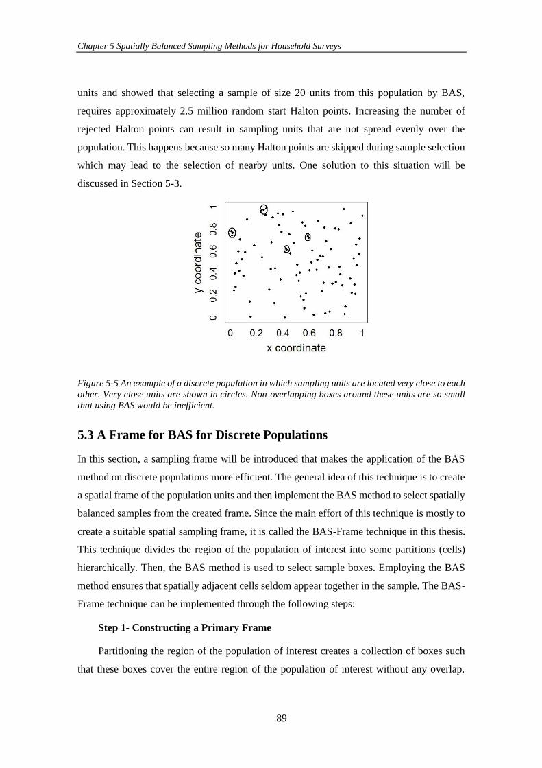
Chapter 5 Spatially Balanced Sampling Methods for Household Surveys
89
units and showed that selecting a sample of size 20 units from this population by BAS,
requires approximately 2.5 million random start Halton points. Increasing the number of
rejected Halton points can result in sampling units that are not spread evenly over the
population. This happens because so many Halton points are skipped during sample selection
which may lead to the selection of nearby units. One solution to this situation will be
discussed in Section 5-3.
Figure 5-5 An example of a discrete population in which sampling units are located very close to each
other. Very close units are shown in circles. Non-overlapping boxes around these units are so small
that using BAS would be inefficient.
5.3 A Frame for BAS for Discrete Populations
In this section, a sampling frame will be introduced that makes the application of the BAS
method on discrete populations more efficient. The general idea of this technique is to create
a spatial frame of the population units and then implement the BAS method to select spatially
balanced samples from the created frame. Since the main effort of this technique is mostly to
create a suitable spatial sampling frame, it is called the BAS-Frame technique in this thesis.
This technique divides the region of the population of interest into some partitions (cells)
hierarchically. Then, the BAS method is used to select sample boxes. Employing the BAS
method ensures that spatially adjacent cells seldom appear together in the sample. The BAS-
Frame technique can be implemented through the following steps:
Step 1- Constructing a Primary Frame
Partitioning the region of the population of interest creates a collection of boxes such
that these boxes cover the entire region of the population of interest without any overlap.
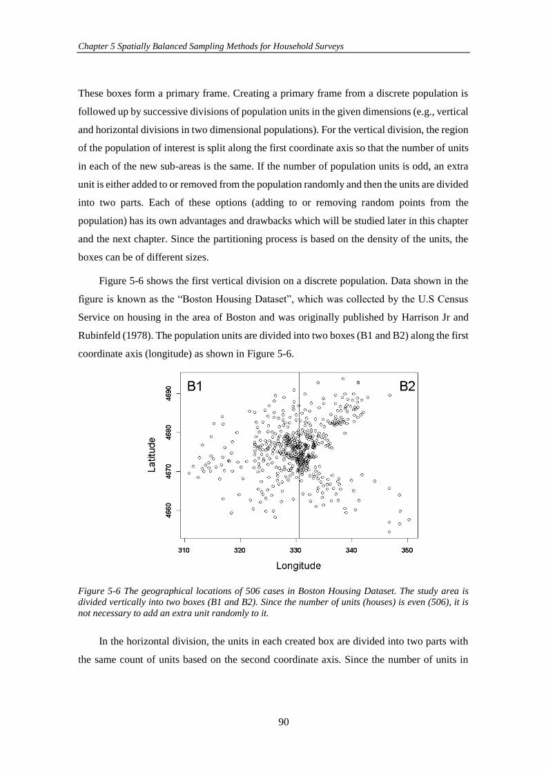
Chapter 5 Spatially Balanced Sampling Methods for Household Surveys
90
These boxes form a primary frame. Creating a primary frame from a discrete population is
followed up by successive divisions of population units in the given dimensions (e.g., vertical
and horizontal divisions in two dimensional populations). For the vertical division, the region
of the population of interest is split along the first coordinate axis so that the number of units
in each of the new sub-areas is the same. If the number of population units is odd, an extra
unit is either added to or removed from the population randomly and then the units are divided
into two parts. Each of these options (adding to or removing random points from the
population) has its own advantages and drawbacks which will be studied later in this chapter
and the next chapter. Since the partitioning process is based on the density of the units, the
boxes can be of different sizes.
Figure 5-6 shows the first vertical division on a discrete population. Data shown in the
figure is known as the “Boston Housing Dataset”, which was collected by the U.S Census
Service on housing in the area of Boston and was originally published by Harrison Jr and
Rubinfeld (1978). The population units are divided into two boxes (B1 and B2) along the first
coordinate axis (longitude) as shown in Figure 5-6.
Figure 5-6 The geographical locations of 506 cases in Boston Housing Dataset. The study area is divided vertically into two boxes (B1 and B2). Since the number of units (houses) is even (506), it is
not necessary to add an extra unit randomly to it.
In the horizontal division, the units in each created box are divided into two parts with
the same count of units based on the second coordinate axis. Since the number of units in
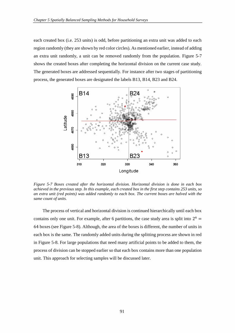
Chapter 5 Spatially Balanced Sampling Methods for Household Surveys
91
each created box (i.e. 253 units) is odd, before partitioning an extra unit was added to each
region randomly (they are shown by red color circles). As mentioned earlier, instead of adding
an extra unit randomly, a unit can be removed randomly from the population. Figure 5-7
shows the created boxes after completing the horizontal division on the current case study.
The generated boxes are addressed sequentially. For instance after two stages of partitioning
process, the generated boxes are designated the labels B13, B14, B23 and B24.
Figure 5-7 Boxes created after the horizontal division. Horizontal division is done in each box
achieved in the previous step. In this example, each created box in the first step contains 253 units, so an extra unit (red points) was added randomly to each box. The current boxes are halved with the
same count of units.
The process of vertical and horizontal division is continued hierarchically until each box
contains only one unit. For example, after 6 partitions, the case study area is split into 26 =
64 boxes (see Figure 5-8). Although, the area of the boxes is different, the number of units in
each box is the same. The randomly added units during the splitting process are shown in red
in Figure 5-8. For large populations that need many artificial points to be added to them, the
process of division can be stopped earlier so that each box contains more than one population
unit. This approach for selecting samples will be discussed later.
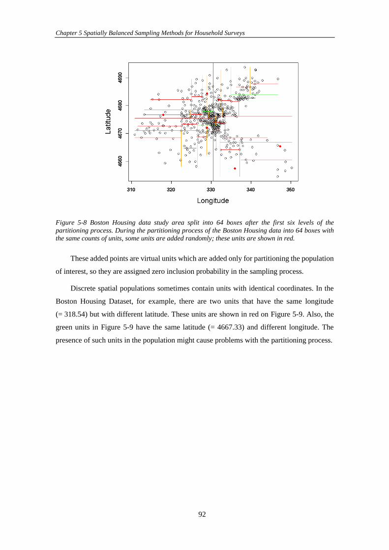
Chapter 5 Spatially Balanced Sampling Methods for Household Surveys
92
Figure 5-8 Boston Housing data study area split into 64 boxes after the first six levels of the
partitioning process. During the partitioning process of the Boston Housing data into 64 boxes with the same counts of units, some units are added randomly; these units are shown in red.
These added points are virtual units which are added only for partitioning the population
of interest, so they are assigned zero inclusion probability in the sampling process.
Discrete spatial populations sometimes contain units with identical coordinates. In the
Boston Housing Dataset, for example, there are two units that have the same longitude
(= 318.54) but with different latitude. These units are shown in red on Figure 5-9. Also, the
green units in Figure 5-9 have the same latitude (= 4667.33) and different longitude. The
presence of such units in the population might cause problems with the partitioning process.
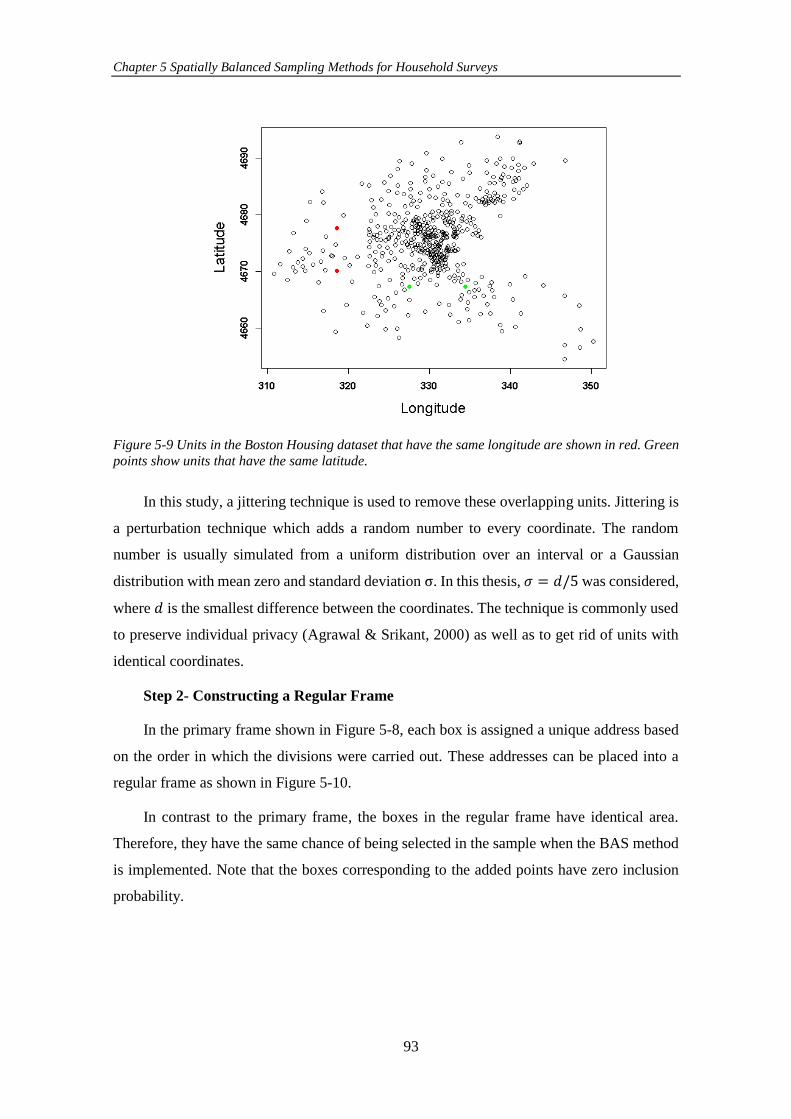
Chapter 5 Spatially Balanced Sampling Methods for Household Surveys
93
Figure 5-9 Units in the Boston Housing dataset that have the same longitude are shown in red. Green
points show units that have the same latitude.
In this study, a jittering technique is used to remove these overlapping units. Jittering is
a perturbation technique which adds a random number to every coordinate. The random
number is usually simulated from a uniform distribution over an interval or a Gaussian
distribution with mean zero and standard deviation σ. In this thesis, 𝜎 = 𝑑/5 was considered,
where 𝑑 is the smallest difference between the coordinates. The technique is commonly used
to preserve individual privacy (Agrawal & Srikant, 2000) as well as to get rid of units with
identical coordinates.
Step 2- Constructing a Regular Frame
In the primary frame shown in Figure 5-8, each box is assigned a unique address based
on the order in which the divisions were carried out. These addresses can be placed into a
regular frame as shown in Figure 5-10.
In contrast to the primary frame, the boxes in the regular frame have identical area.
Therefore, they have the same chance of being selected in the sample when the BAS method
is implemented. Note that the boxes corresponding to the added points have zero inclusion
probability.
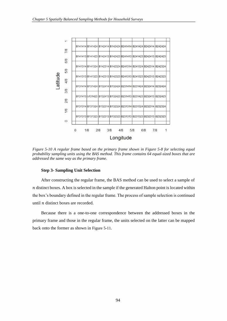
Chapter 5 Spatially Balanced Sampling Methods for Household Surveys
94
Figure 5-10 A regular frame based on the primary frame shown in Figure 5-8 for selecting equal
probability sampling units using the BAS method. This frame contains 64 equal-sized boxes that are
addressed the same way as the primary frame.
Step 3- Sampling Unit Selection
After constructing the regular frame, the BAS method can be used to select a sample of
𝑛 distinct boxes. A box is selected in the sample if the generated Halton point is located within
the box’s boundary defined in the regular frame. The process of sample selection is continued
until 𝑛 distinct boxes are recorded.
Because there is a one-to-one correspondence between the addressed boxes in the
primary frame and those in the regular frame, the units selected on the latter can be mapped
back onto the former as shown in Figure 5-11.
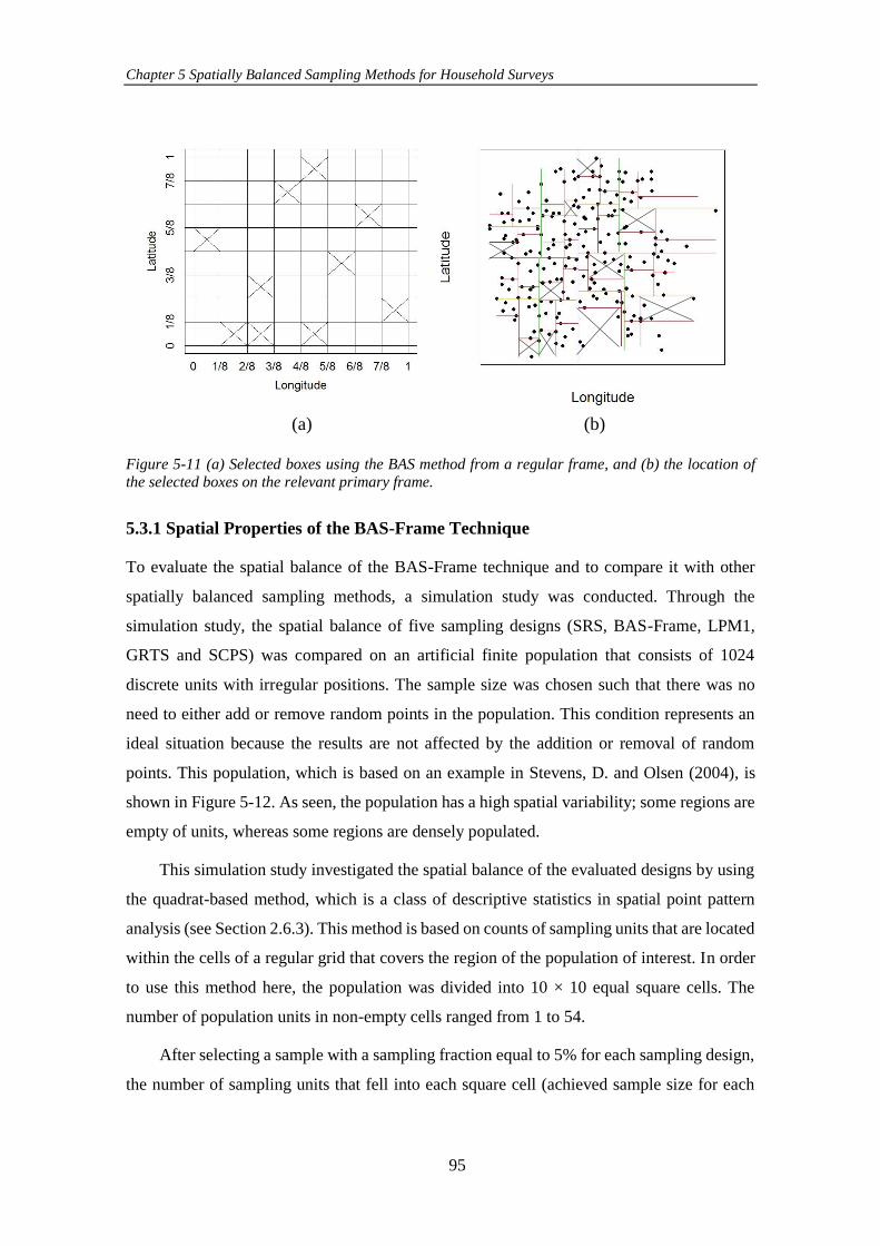
Chapter 5 Spatially Balanced Sampling Methods for Household Surveys
95
Figure 5-11 (a) Selected boxes using the BAS method from a regular frame, and (b) the location of the selected boxes on the relevant primary frame.
5.3.1 Spatial Properties of the BAS-Frame Technique
To evaluate the spatial balance of the BAS-Frame technique and to compare it with other
spatially balanced sampling methods, a simulation study was conducted. Through the
simulation study, the spatial balance of five sampling designs (SRS, BAS-Frame, LPM1,
GRTS and SCPS) was compared on an artificial finite population that consists of 1024
discrete units with irregular positions. The sample size was chosen such that there was no
need to either add or remove random points in the population. This condition represents an
ideal situation because the results are not affected by the addition or removal of random
points. This population, which is based on an example in Stevens, D. and Olsen (2004), is
shown in Figure 5-12. As seen, the population has a high spatial variability; some regions are
empty of units, whereas some regions are densely populated.
This simulation study investigated the spatial balance of the evaluated designs by using
the quadrat-based method, which is a class of descriptive statistics in spatial point pattern
analysis (see Section 2.6.3). This method is based on counts of sampling units that are located
within the cells of a regular grid that covers the region of the population of interest. In order
to use this method here, the population was divided into 10 × 10 equal square cells. The
number of population units in non-empty cells ranged from 1 to 54.
After selecting a sample with a sampling fraction equal to 5% for each sampling design,
the number of sampling units that fell into each square cell (achieved sample size for each
(a) (b)
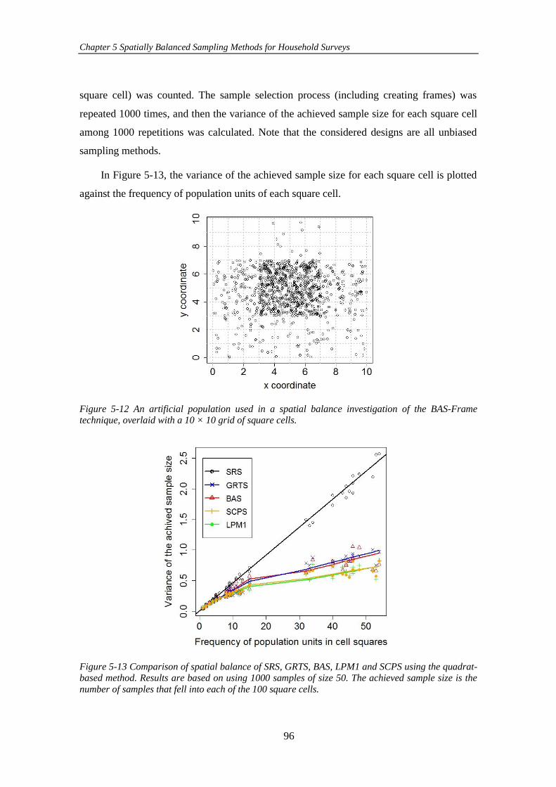
Chapter 5 Spatially Balanced Sampling Methods for Household Surveys
96
square cell) was counted. The sample selection process (including creating frames) was
repeated 1000 times, and then the variance of the achieved sample size for each square cell
among 1000 repetitions was calculated. Note that the considered designs are all unbiased
sampling methods.
In Figure 5-13, the variance of the achieved sample size for each square cell is plotted
against the frequency of population units of each square cell.
Figure 5-12 An artificial population used in a spatial balance investigation of the BAS-Frame technique, overlaid with a 10 × 10 grid of square cells.
Figure 5-13 Comparison of spatial balance of SRS, GRTS, BAS, LPM1 and SCPS using the quadrat-based method. Results are based on using 1000 samples of size 50. The achieved sample size is the
number of samples that fell into each of the 100 square cells.
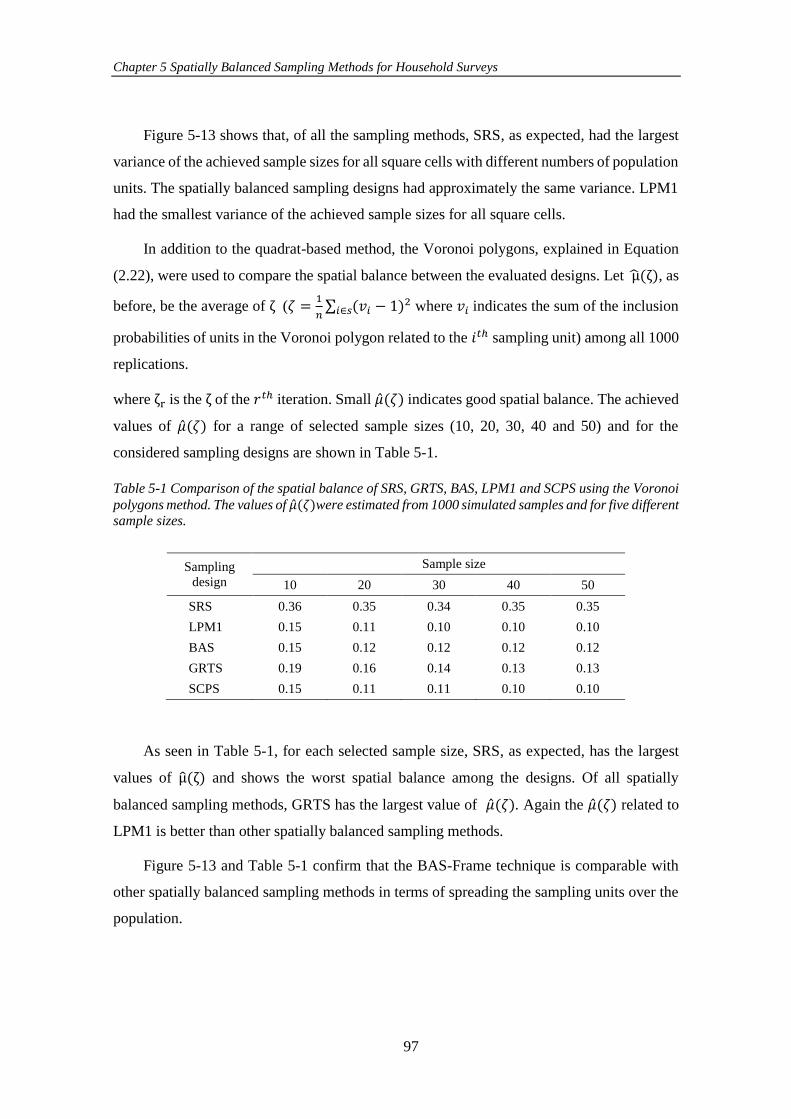
Chapter 5 Spatially Balanced Sampling Methods for Household Surveys
97
Figure 5-13 shows that, of all the sampling methods, SRS, as expected, had the largest
variance of the achieved sample sizes for all square cells with different numbers of population
units. The spatially balanced sampling designs had approximately the same variance. LPM1
had the smallest variance of the achieved sample sizes for all square cells.
In addition to the quadrat-based method, the Voronoi polygons, explained in Equation
(2.22), were used to compare the spatial balance between the evaluated designs. Let μ(ζ), as
before, be the average of ζ (𝜁 =1
𝑛∑ (𝑣𝑖 − 1)
2𝑖∈𝑠 where 𝑣𝑖 indicates the sum of the inclusion
probabilities of units in the Voronoi polygon related to the 𝑖𝑡ℎ sampling unit) among all 1000
replications.
where ζr is the ζ of the 𝑟𝑡ℎ iteration. Small ��(𝜁) indicates good spatial balance. The achieved
values of ��(𝜁) for a range of selected sample sizes (10, 20, 30, 40 and 50) and for the
considered sampling designs are shown in Table 5-1.
Table 5-1 Comparison of the spatial balance of SRS, GRTS, BAS, LPM1 and SCPS using the Voronoi
polygons method. The values of ��(𝜁)were estimated from 1000 simulated samples and for five different sample sizes.
Sampling
design
Sample size
10 20 30 40 50
SRS 0.36 0.35 0.34 0.35 0.35
LPM1 0.15 0.11 0.10 0.10 0.10
BAS 0.15 0.12 0.12 0.12 0.12
GRTS 0.19 0.16 0.14 0.13 0.13
SCPS 0.15 0.11 0.11 0.10 0.10
As seen in Table 5-1, for each selected sample size, SRS, as expected, has the largest
values of μ(ζ) and shows the worst spatial balance among the designs. Of all spatially
balanced sampling methods, GRTS has the largest value of ��(𝜁). Again the ��(𝜁) related to
LPM1 is better than other spatially balanced sampling methods.
Figure 5-13 and Table 5-1 confirm that the BAS-Frame technique is comparable with
other spatially balanced sampling methods in terms of spreading the sampling units over the
population.
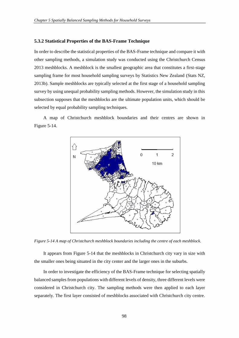
Chapter 5 Spatially Balanced Sampling Methods for Household Surveys
98
5.3.2 Statistical Properties of the BAS-Frame Technique
In order to describe the statistical properties of the BAS-Frame technique and compare it with
other sampling methods, a simulation study was conducted using the Christchurch Census
2013 meshblocks. A meshblock is the smallest geographic area that constitutes a first-stage
sampling frame for most household sampling surveys by Statistics New Zealand (Stats NZ,
2013b). Sample meshblocks are typically selected at the first stage of a household sampling
survey by using unequal probability sampling methods. However, the simulation study in this
subsection supposes that the meshblocks are the ultimate population units, which should be
selected by equal probability sampling techniques.
A map of Christchurch meshblock boundaries and their centres are shown in
Figure 5-14.
Figure 5-14 A map of Christchurch meshblock boundaries including the centre of each meshblock.
It appears from Figure 5-14 that the meshblocks in Christchurch city vary in size with
the smaller ones being situated in the city center and the larger ones in the suburbs.
In order to investigate the efficiency of the BAS-Frame technique for selecting spatially
balanced samples from populations with different levels of density, three different levels were
considered in Christchurch city. The sampling methods were then applied to each layer
separately. The first layer consisted of meshblocks associated with Christchurch city centre.
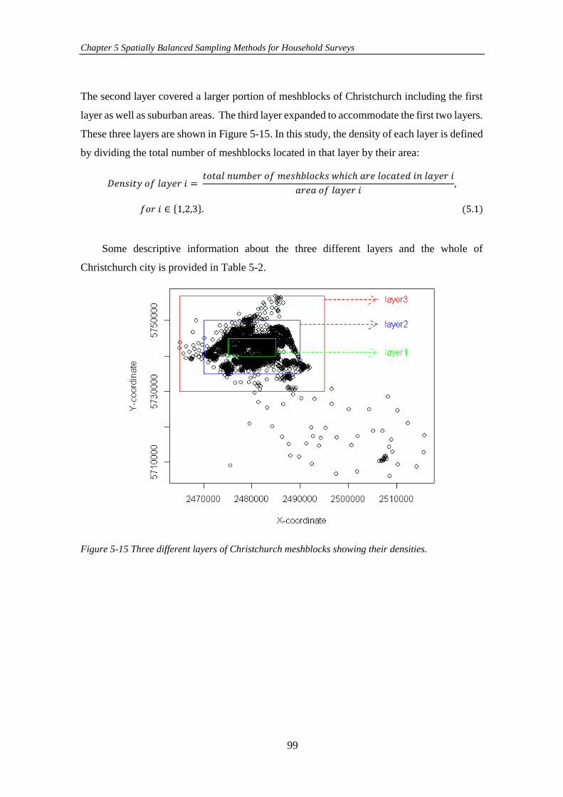
Chapter 5 Spatially Balanced Sampling Methods for Household Surveys
99
The second layer covered a larger portion of meshblocks of Christchurch including the first
layer as well as suburban areas. The third layer expanded to accommodate the first two layers.
These three layers are shown in Figure 5-15. In this study, the density of each layer is defined
by dividing the total number of meshblocks located in that layer by their area:
𝐷𝑒𝑛𝑠𝑖𝑡𝑦 𝑜𝑓 𝑙𝑎𝑦𝑒𝑟 𝑖 = 𝑡𝑜𝑡𝑎𝑙 𝑛𝑢𝑚𝑏𝑒𝑟 𝑜𝑓 𝑚𝑒𝑠ℎ𝑏𝑙𝑜𝑐𝑘𝑠 𝑤ℎ𝑖𝑐ℎ 𝑎𝑟𝑒 𝑙𝑜𝑐𝑎𝑡𝑒𝑑 𝑖𝑛 𝑙𝑎𝑦𝑒𝑟 𝑖
𝑎𝑟𝑒𝑎 𝑜𝑓 𝑙𝑎𝑦𝑒𝑟 𝑖,
𝑓𝑜𝑟 𝑖 ∈ {1,2,3}. (5.1)
Some descriptive information about the three different layers and the whole of
Christchurch city is provided in Table 5-2.
Figure 5-15 Three different layers of Christchurch meshblocks showing their densities.
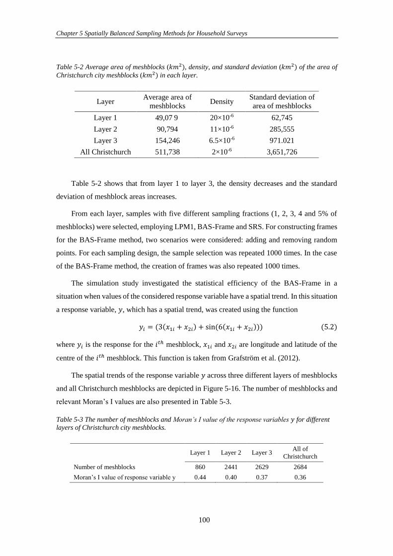
Chapter 5 Spatially Balanced Sampling Methods for Household Surveys
100
Table 5-2 Average area of meshblocks (𝑘𝑚2), density, and standard deviation (𝑘𝑚2) of the area of
Christchurch city meshblocks (𝑘𝑚2) in each layer.
Layer Average area of
meshblocks Density
Standard deviation of
area of meshblocks
Layer 1 49,07 9 20×10-6 62,745
Layer 2 90,794 11×10-6 285,555
Layer 3 154,246 6.5×10⁻⁶ 971.021
All Christchurch 511,738 2×10⁻⁶ 3,651,726
Table 5-2 shows that from layer 1 to layer 3, the density decreases and the standard
deviation of meshblock areas increases.
From each layer, samples with five different sampling fractions (1, 2, 3, 4 and 5% of
meshblocks) were selected, employing LPM1, BAS-Frame and SRS. For constructing frames
for the BAS-Frame method, two scenarios were considered: adding and removing random
points. For each sampling design, the sample selection was repeated 1000 times. In the case
of the BAS-Frame method, the creation of frames was also repeated 1000 times.
The simulation study investigated the statistical efficiency of the BAS-Frame in a
situation when values of the considered response variable have a spatial trend. In this situation
a response variable, 𝑦, which has a spatial trend, was created using the function
𝑦𝑖 = (3(𝑥1𝑖 + 𝑥2𝑖) + sin(6(𝑥1𝑖 + 𝑥2𝑖))) (5.2)
where 𝑦𝑖 is the response for the 𝑖𝑡ℎ meshblock, 𝑥1𝑖 and 𝑥2𝑖 are longitude and latitude of the
centre of the 𝑖𝑡ℎ meshblock. This function is taken from Grafström et al. (2012).
The spatial trends of the response variable 𝑦 across three different layers of meshblocks
and all Christchurch meshblocks are depicted in Figure 5-16. The number of meshblocks and
relevant Moran’s I values are also presented in Table 5-3.
Table 5-3 The number of meshblocks and Moran’s I value of the response variables 𝑦 for different
layers of Christchurch city meshblocks.
Layer 1 Layer 2 Layer 3 All of
Christchurch
Number of meshblocks 860 2441 2629 2684
Moran’s I value of response variable y 0.44 0.40 0.37 0.36
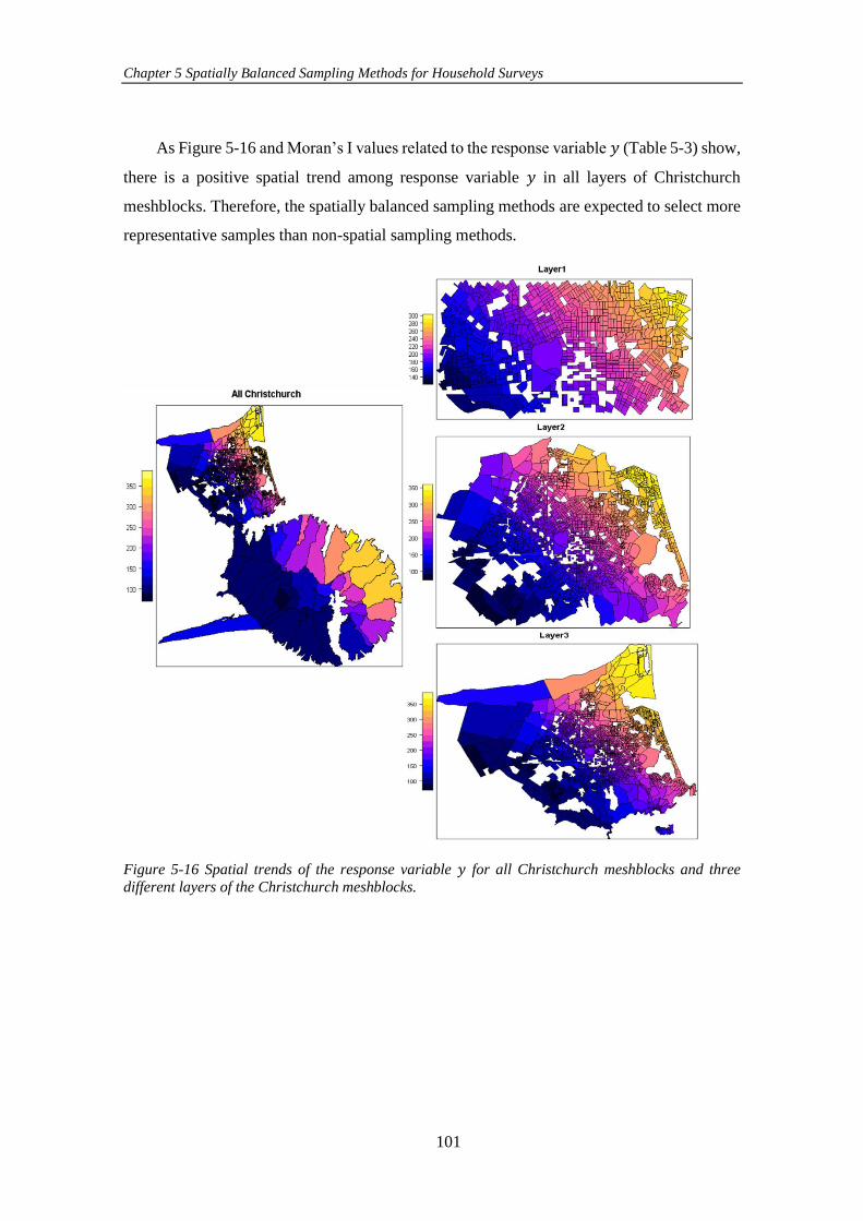
Chapter 5 Spatially Balanced Sampling Methods for Household Surveys
101
As Figure 5-16 and Moran’s I values related to the response variable 𝑦 (Table 5-3) show,
there is a positive spatial trend among response variable 𝑦 in all layers of Christchurch
meshblocks. Therefore, the spatially balanced sampling methods are expected to select more
representative samples than non-spatial sampling methods.
Figure 5-16 Spatial trends of the response variable 𝑦 for all Christchurch meshblocks and three
different layers of the Christchurch meshblocks.
Chapter 5 Spatially Balanced Sampling Methods for Household Surveys
102
After selecting 1000 samples from each sampling scheme, the variance of the HT
estimator was simulated:
��(��𝐻𝑇) =1
1000∑(��𝐻𝑇𝑖 − 𝑇)
21000
𝑖=1
(5.3)
where ��𝐻𝑇_𝑖 is the total value of the response variable, which is estimated from the 𝑖𝑡ℎ iteration
and 𝑇 is the true total value of the response variable.
In this study, the total value of the response variable (𝑇 = ∑ 𝑦𝑖𝑖 ) is known for each layer.
Regarding the simulated ��(��𝐻𝑇), 𝐷𝑒𝑓𝑓 was estimated for each sampling design using
the following equation:
𝐷𝑒𝑓𝑓 =V(THT−𝐶𝑜𝑚𝑝𝑙𝑒𝑥 𝑆𝑢𝑟𝑣𝑒𝑦)
V(TSRS). (5.4)
The results of the simulation study for estimating the response variable 𝑦 are shown in
Table 5-4. The average of 𝜁 (according to Equation (2.22)) among all 1000 replicates (��(𝜁))
is also reported in Table 5-4 as an index of spatial balance created by each sampling design.
Table 5-4 shows that for all sampling fractions and in all considered layers, the 𝐷𝑒𝑓𝑓
related to the spatially balanced sampling methods are smaller than 1. This shows that the
spatially balanced sampling methods estimated the total value of the response variable (��𝐻𝑇)
with a variance that was smaller than the variance of the SRS method. Therefore, the spatially
balanced sampling methods are more precise than SRS in terms of estimating the population
parameters. Table 5-4 shows that there is no remarkable difference between results in the
different layers considered. It confirms that the spatially balanced sampling methods can
select precise samples from populations with different levels of density. Findings from
Table 5-4 indicate that the BAS-Frame method can work as precisely as other spatially
balanced sampling methods. Comparing two scenarios (adding or removing random points)
for implementing the BAS-Frame method, it was found that the removal of random points
results in samples which are more spatially balanced. In this example, the population units
had the same inclusion probability; therefore removing points randomly did not change the
probability of selection of the population units. The values of μ(ζ) indicate that LPM1
provides more spatially balanced samples when compared to other methods.
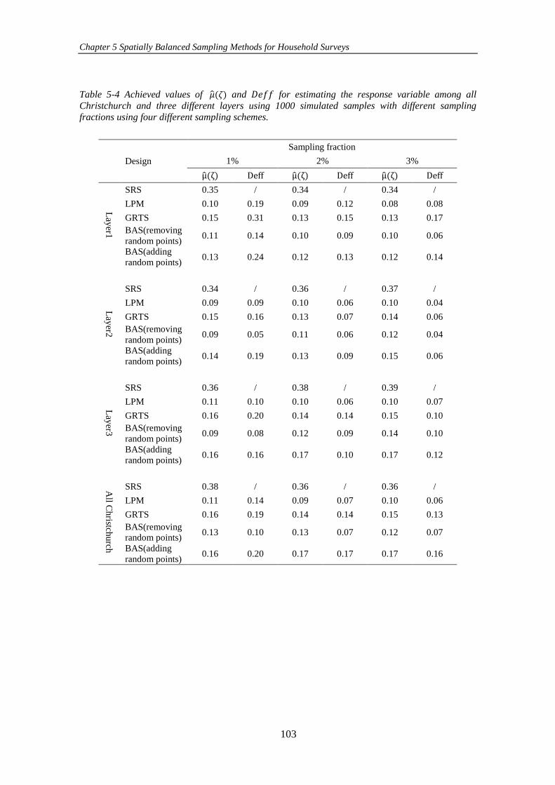
Chapter 5 Spatially Balanced Sampling Methods for Household Surveys
103
Table 5-4 Achieved values of ��(𝜁) and 𝐷𝑒𝑓𝑓 for estimating the response variable among all
Christchurch and three different layers using 1000 simulated samples with different sampling
fractions using four different sampling schemes.
Design
Sampling fraction
1% 2% 3%
μ(ζ) Deff μ(ζ) Deff μ(ζ) Deff
Lay
er1
SRS 0.35 / 0.34 / 0.34 /
LPM 0.10 0.19 0.09 0.12 0.08 0.08
GRTS 0.15 0.31 0.13 0.15 0.13 0.17
BAS(removing
random points) 0.11 0.14 0.10 0.09 0.10 0.06
BAS(adding
random points) 0.13 0.24 0.12 0.13 0.12 0.14
Lay
er2
SRS 0.34 / 0.36 / 0.37 /
LPM 0.09 0.09 0.10 0.06 0.10 0.04
GRTS 0.15 0.16 0.13 0.07 0.14 0.06
BAS(removing
random points) 0.09 0.05 0.11 0.06 0.12 0.04
BAS(adding
random points) 0.14 0.19 0.13 0.09 0.15 0.06
Lay
er3
SRS 0.36 / 0.38 / 0.39 /
LPM 0.11 0.10 0.10 0.06 0.10 0.07
GRTS 0.16 0.20 0.14 0.14 0.15 0.10
BAS(removing
random points) 0.09 0.08 0.12 0.09 0.14 0.10
BAS(adding
random points) 0.16 0.16 0.17 0.10 0.17 0.12
All C
hristch
urch
SRS 0.38 / 0.36 / 0.36 /
LPM 0.11 0.14 0.09 0.07 0.10 0.06
GRTS 0.16 0.19 0.14 0.14 0.15 0.13
BAS(removing
random points) 0.13 0.10 0.13 0.07 0.12 0.07
BAS(adding
random points) 0.16 0.20 0.17 0.17 0.17 0.16
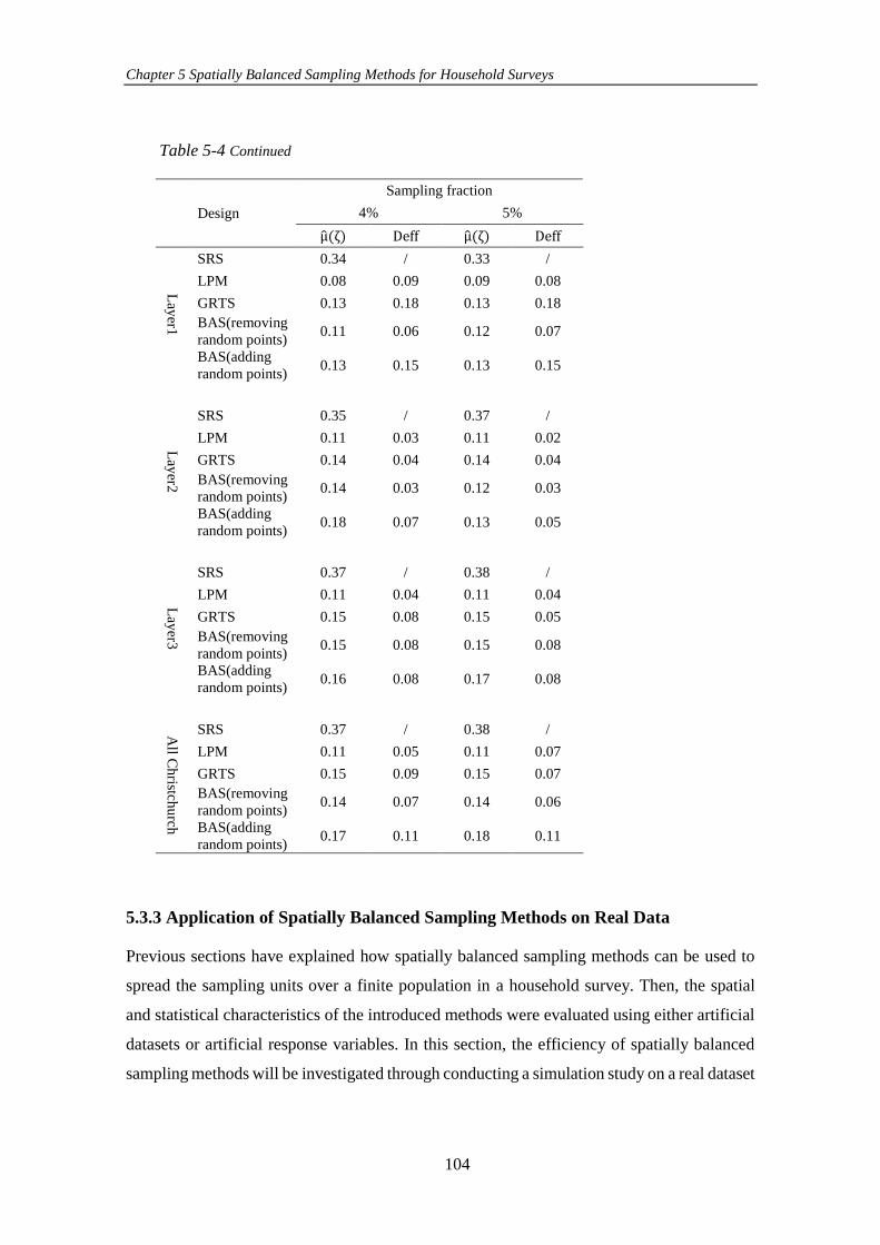
Chapter 5 Spatially Balanced Sampling Methods for Household Surveys
104
Table 5-4 Continued
Design
Sampling fraction
4% 5%
μ(ζ) Deff μ(ζ) Deff
Lay
er1
SRS 0.34 / 0.33 /
LPM 0.08 0.09 0.09 0.08
GRTS 0.13 0.18 0.13 0.18
BAS(removing
random points) 0.11 0.06 0.12 0.07
BAS(adding
random points) 0.13 0.15 0.13 0.15
Lay
er2
SRS 0.35 / 0.37 /
LPM 0.11 0.03 0.11 0.02
GRTS 0.14 0.04 0.14 0.04
BAS(removing
random points) 0.14 0.03 0.12 0.03
BAS(adding
random points) 0.18 0.07 0.13 0.05
Lay
er3
SRS 0.37 / 0.38 /
LPM 0.11 0.04 0.11 0.04
GRTS 0.15 0.08 0.15 0.05
BAS(removing
random points) 0.15 0.08 0.15 0.08
BAS(adding
random points) 0.16 0.08 0.17 0.08
A
ll Ch
ristchu
rch
SRS 0.37 / 0.38 /
LPM 0.11 0.05 0.11 0.07
GRTS 0.15 0.09 0.15 0.07
BAS(removing
random points) 0.14 0.07 0.14 0.06
BAS(adding
random points) 0.17 0.11 0.18 0.11
5.3.3 Application of Spatially Balanced Sampling Methods on Real Data
Previous sections have explained how spatially balanced sampling methods can be used to
spread the sampling units over a finite population in a household survey. Then, the spatial
and statistical characteristics of the introduced methods were evaluated using either artificial
datasets or artificial response variables. In this section, the efficiency of spatially balanced
sampling methods will be investigated through conducting a simulation study on a real dataset
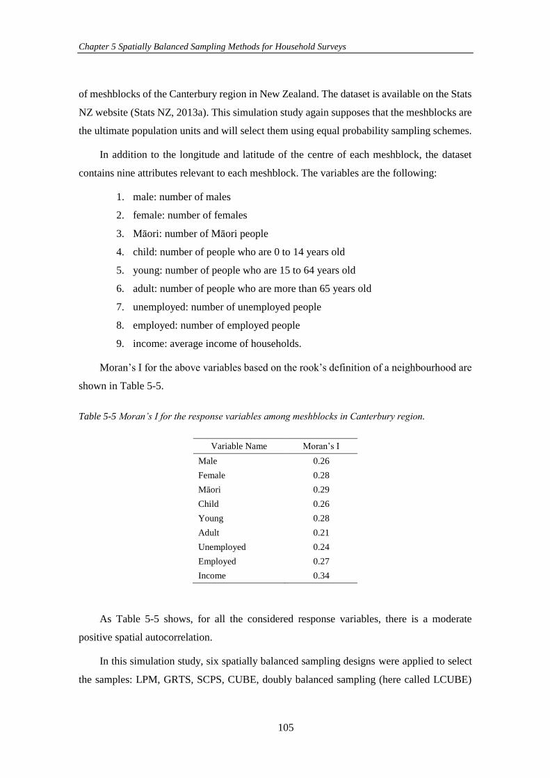
Chapter 5 Spatially Balanced Sampling Methods for Household Surveys
105
of meshblocks of the Canterbury region in New Zealand. The dataset is available on the Stats
NZ website (Stats NZ, 2013a). This simulation study again supposes that the meshblocks are
the ultimate population units and will select them using equal probability sampling schemes.
In addition to the longitude and latitude of the centre of each meshblock, the dataset
contains nine attributes relevant to each meshblock. The variables are the following:
1. male: number of males
2. female: number of females
3. Māori: number of Māori people
4. child: number of people who are 0 to 14 years old
5. young: number of people who are 15 to 64 years old
6. adult: number of people who are more than 65 years old
7. unemployed: number of unemployed people
8. employed: number of employed people
9. income: average income of households.
Moran’s I for the above variables based on the rook’s definition of a neighbourhood are
shown in Table 5-5.
Table 5-5 Moran’s I for the response variables among meshblocks in Canterbury region.
Variable Name Moran’s I
Male 0.26
Female 0.28
Māori 0.29
Child 0.26
Young 0.28
Adult 0.21
Unemployed 0.24
Employed 0.27
Income 0.34
As Table 5-5 shows, for all the considered response variables, there is a moderate
positive spatial autocorrelation.
In this simulation study, six spatially balanced sampling designs were applied to select
the samples: LPM, GRTS, SCPS, CUBE, doubly balanced sampling (here called LCUBE)
Chapter 5 Spatially Balanced Sampling Methods for Household Surveys
106
and BAS-Frame. Two scenarios were considered for the BAS-Frame method: adding and
removing random points. SRS was also used as a benchmark for comparing the spatially
balanced sampling methods. For selecting spatially balanced samples using the CUBE and
LCUBE methods, the coordinates of the centres of the meshblocks were considered as
balanced variables. As in other simulation studies that have been conducted in this thesis, a
range of five different sampling fractions was considered: 1, 2, 3, 4 and 5% of the meshblocks.
After selecting 1000 samples for each sampling method and calculating the variance of
the HT estimator for estimating the mean of each response variable, the 𝐷𝑒𝑓𝑓 relevant to
each sampling design was calculated using Equation (2.12). Results of the simulation study
for estimating the mean of the response variables for different sampling fractions are
reported in Table 5-6.
Table 5-7 also reports the average of 𝐷𝑒𝑓𝑓 (over all variables) for each sampling design.
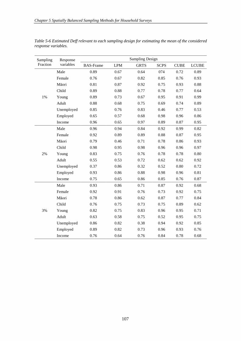
Chapter 5 Spatially Balanced Sampling Methods for Household Surveys
107
Table 5-6 Estimated Deff relevant to each sampling design for estimating the mean of the considered
response variables.
Sampling
Fraction
Response
variables
Sampling Design
BAS-Frame LPM GRTS SCPS CUBE LCUBE
1%
Male 0.89 0.67 0.64 074 0.72 0.89
Female 0.76 0.67 0.82 0.85 0.76 0.93
Māori 0.81 0.87 0.92 0.75 0.93 0.88
Child 0.89 0.88 0.77 0.78 0.77 0.64
Young 0.89 0.73 0.67 0.95 0.91 0.99
Adult 0.88 0.68 0.75 0.69 0.74 0.89
Unemployed 0.85 0.76 0.83 0.46 0.77 0.53
Employed 0.65 0.57 0.68 0.98 0.96 0.86
Income 0.96 0.65 0.97 0.89 0.87 0.95
2%
Male 0.96 0.94 0.84 0.92 0.99 0.82
Female 0.92 0.89 0.89 0.88 0.87 0.95
Māori 0.79 0.46 0.71 0.78 0.86 0.93
Child 0.98 0.95 0.98 0.96 0.96 0.97
Young 0.83 0.75 0.76 0.78 0.78 0.80
Adult 0.55 0.53 0.72 0.62 0.62 0.92
Unemployed 0.37 0.86 0.32 0.52 0.80 0.72
Employed 0.93 0.86 0.88 0.98 0.96 0.81
Income 0.75 0.65 0.86 0.85 0.76 0.87
3%
Male 0.93 0.86 0.71 0.87 0.92 0.68
Female 0.92 0.91 0.76 0.73 0.92 0.75
Māori 0.78 0.86 0.62 0.87 0.77 0.84
Child 0.76 0.75 0.73 0.75 0.89 0.62
Young 0.82 0.75 0.83 0.96 0.95 0.71
Adult 0.63 0.58 0.75 0.52 0.95 0.75
Unemployed 0.86 0.82 0.38 0.94 0.92 0.85
Employed 0.89 0.82 0.73 0.96 0.93 0.76
Income 0.76 0.64 0.76 0.84 0.78 0.68
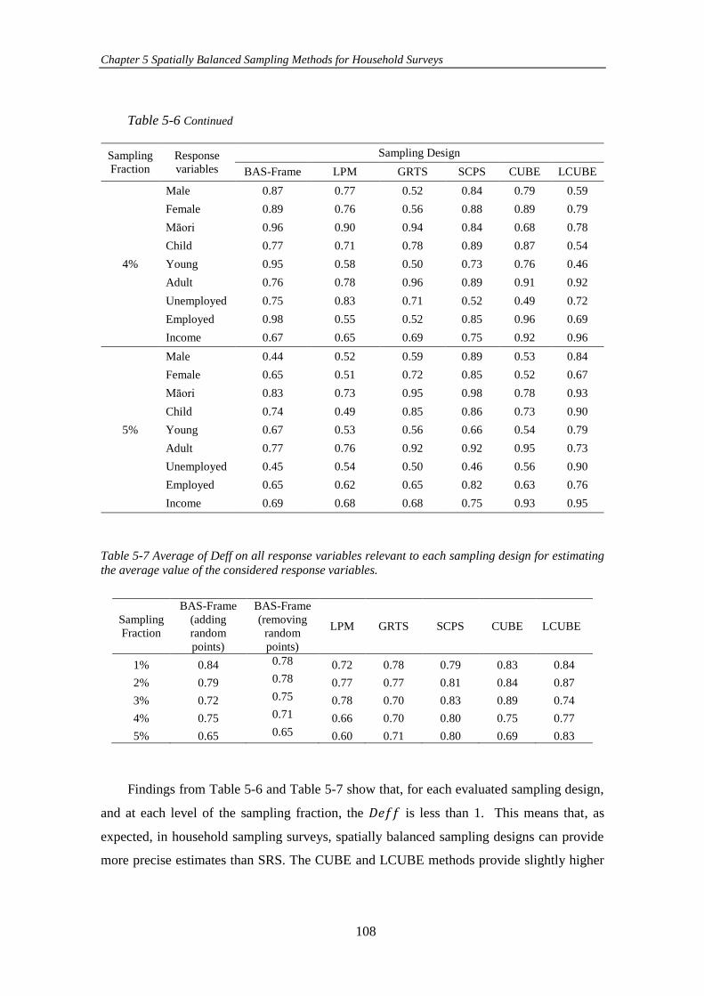
Chapter 5 Spatially Balanced Sampling Methods for Household Surveys
108
Table 5-6 Continued
Sampling
Fraction
Response
variables
Sampling Design
BAS-Frame LPM GRTS SCPS CUBE LCUBE
4%
Male 0.87 0.77 0.52 0.84 0.79 0.59
Female 0.89 0.76 0.56 0.88 0.89 0.79
Māori 0.96 0.90 0.94 0.84 0.68 0.78
Child 0.77 0.71 0.78 0.89 0.87 0.54
Young 0.95 0.58 0.50 0.73 0.76 0.46
Adult 0.76 0.78 0.96 0.89 0.91 0.92
Unemployed 0.75 0.83 0.71 0.52 0.49 0.72
Employed 0.98 0.55 0.52 0.85 0.96 0.69
Income 0.67 0.65 0.69 0.75 0.92 0.96
5%
Male 0.44 0.52 0.59 0.89 0.53 0.84
Female 0.65 0.51 0.72 0.85 0.52 0.67
Māori 0.83 0.73 0.95 0.98 0.78 0.93
Child 0.74 0.49 0.85 0.86 0.73 0.90
Young 0.67 0.53 0.56 0.66 0.54 0.79
Adult 0.77 0.76 0.92 0.92 0.95 0.73
Unemployed 0.45 0.54 0.50 0.46 0.56 0.90
Employed 0.65 0.62 0.65 0.82 0.63 0.76
Income 0.69 0.68 0.68 0.75 0.93 0.95
Table 5-7 Average of Deff on all response variables relevant to each sampling design for estimating
the average value of the considered response variables.
Sampling
Fraction
BAS-Frame
(adding
random
points)
BAS-Frame
(removing
random
points)
LPM GRTS SCPS CUBE LCUBE
1% 0.84 0.78 0.72 0.78 0.79 0.83 0.84
2% 0.79 0.78 0.77 0.77 0.81 0.84 0.87
3% 0.72 0.75 0.78 0.70 0.83 0.89 0.74
4% 0.75 0.71 0.66 0.70 0.80 0.75 0.77
5% 0.65 0.65 0.60 0.71 0.80 0.69 0.83
Findings from Table 5-6 and Table 5-7 show that, for each evaluated sampling design,
and at each level of the sampling fraction, the 𝐷𝑒𝑓𝑓 is less than 1. This means that, as
expected, in household sampling surveys, spatially balanced sampling designs can provide
more precise estimates than SRS. The CUBE and LCUBE methods provide slightly higher
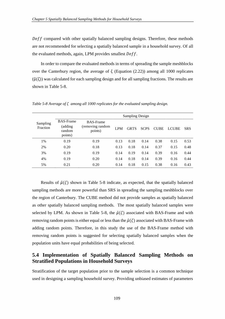
Chapter 5 Spatially Balanced Sampling Methods for Household Surveys
109
𝐷𝑒𝑓𝑓 compared with other spatially balanced sampling designs. Therefore, these methods
are not recommended for selecting a spatially balanced sample in a household survey. Of all
the evaluated methods, again, LPM provides smallest 𝐷𝑒𝑓𝑓.
In order to compare the evaluated methods in terms of spreading the sample meshblocks
over the Canterbury region, the average of ζ (Equation (2.22)) among all 1000 replicates
(μ(ζ)) was calculated for each sampling design and for all sampling fractions. The results are
shown in Table 5-8.
Table 5-8 Average of 𝜁 among all 1000 replicates for the evaluated sampling design.
Sampling
Fraction
Sampling Design
BAS-Frame
(adding
random
points)
BAS-Frame
(removing random
points) LPM GRTS SCPS CUBE LCUBE SRS
1% 0.19 0.19 0.13 0.18 0.14 0.38 0.15 0.53
2% 0.20 0.18 0.13 0.18 0.14 0.37 0.15 0.48
3% 0.19 0.19 0.14 0.19 0.14 0.39 0.16 0.44
4% 0.19 0.20 0.14 0.18 0.14 0.39 0.16 0.44
5% 0.21 0.20 0.14 0.18 0.15 0.38 0.16 0.43
Results of ��(𝜁) shown in Table 5-8 indicate, as expected, that the spatially balanced
sampling methods are more powerful than SRS in spreading the sampling meshblocks over
the region of Canterbury. The CUBE method did not provide samples as spatially balanced
as other spatially balanced sampling methods. The most spatially balanced samples were
selected by LPM. As shown in Table 5-8, the ��(𝜁) associated with BAS-Frame and with
removing random points is either equal or less than the ��(𝜁) associated with BAS-Frame with
adding random points. Therefore, in this study the use of the BAS-Frame method with
removing random points is suggested for selecting spatially balanced samples when the
population units have equal probabilities of being selected.
5.4 Implementation of Spatially Balanced Sampling Methods on
Stratified Populations in Household Surveys
Stratification of the target population prior to the sample selection is a common technique
used in designing a sampling household survey. Providing unbiased estimates of parameters
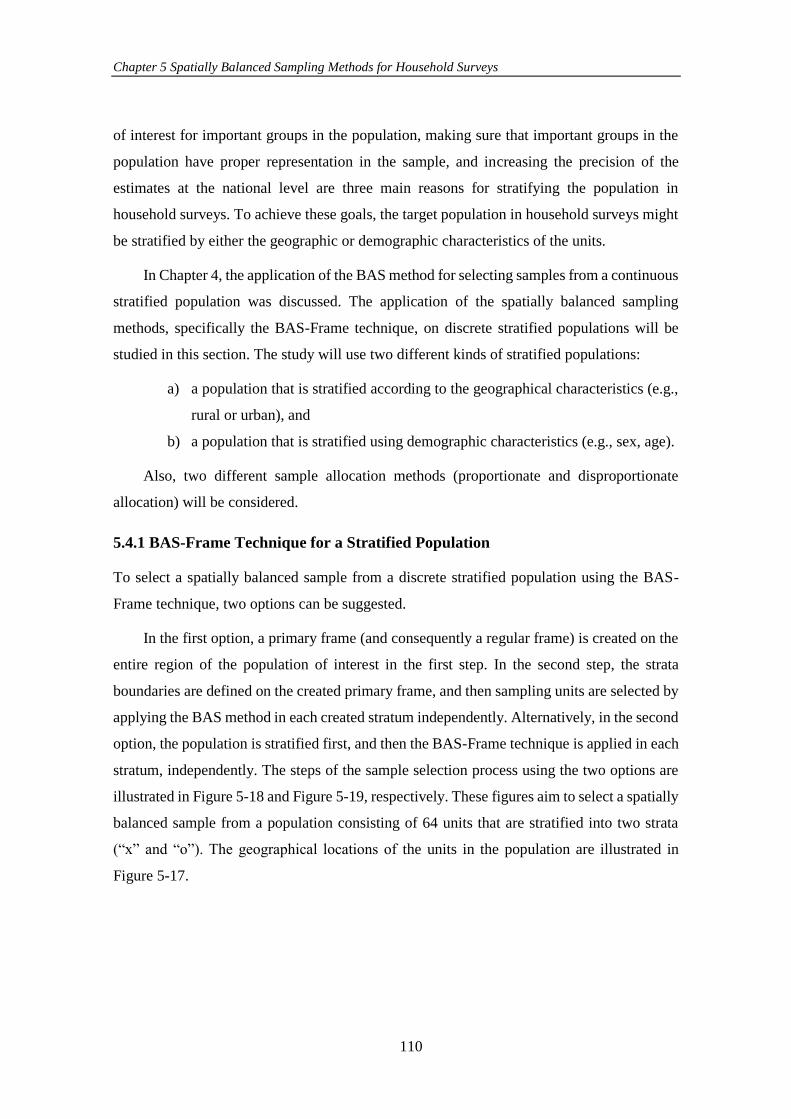
Chapter 5 Spatially Balanced Sampling Methods for Household Surveys
110
of interest for important groups in the population, making sure that important groups in the
population have proper representation in the sample, and increasing the precision of the
estimates at the national level are three main reasons for stratifying the population in
household surveys. To achieve these goals, the target population in household surveys might
be stratified by either the geographic or demographic characteristics of the units.
In Chapter 4, the application of the BAS method for selecting samples from a continuous
stratified population was discussed. The application of the spatially balanced sampling
methods, specifically the BAS-Frame technique, on discrete stratified populations will be
studied in this section. The study will use two different kinds of stratified populations:
a) a population that is stratified according to the geographical characteristics (e.g.,
rural or urban), and
b) a population that is stratified using demographic characteristics (e.g., sex, age).
Also, two different sample allocation methods (proportionate and disproportionate
allocation) will be considered.
5.4.1 BAS-Frame Technique for a Stratified Population
To select a spatially balanced sample from a discrete stratified population using the BAS-
Frame technique, two options can be suggested.
In the first option, a primary frame (and consequently a regular frame) is created on the
entire region of the population of interest in the first step. In the second step, the strata
boundaries are defined on the created primary frame, and then sampling units are selected by
applying the BAS method in each created stratum independently. Alternatively, in the second
option, the population is stratified first, and then the BAS-Frame technique is applied in each
stratum, independently. The steps of the sample selection process using the two options are
illustrated in Figure 5-18 and Figure 5-19, respectively. These figures aim to select a spatially
balanced sample from a population consisting of 64 units that are stratified into two strata
(“x” and “o”). The geographical locations of the units in the population are illustrated in
Figure 5-17.
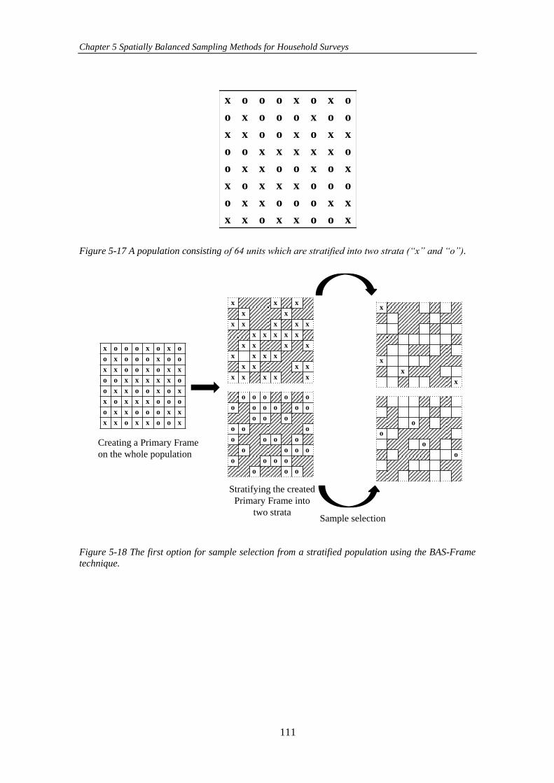
Chapter 5 Spatially Balanced Sampling Methods for Household Surveys
111
Figure 5-17 A population consisting of 64 units which are stratified into two strata (“x” and “o”).
Figure 5-18 The first option for sample selection from a stratified population using the BAS-Frame
technique.
x o o o x o x o
o x o o o x o o
x x o o x o x x
o o x x x x x o
o x x o o x o x
x o x x x o o o
o x x o o o x x
x x o x x o o x
x o o o x o x o
o x o o o x o o
x x o o x o x x
o o x x x x x o
o x x o o x o x
x o x x x o o o
o x x o o o x x
x x o x x o o x
x x x
x x
x x x x x
x x x x x
x x x x
x x x x
x x x x
x x x x x
o o o o o
o o o o o o
o o o
o o o
o o o o
o o o o
o o o o
o o o
Creating a Primary Frame
on the whole population
Sample selection
Stratifying the created
Primary Frame into
two strata
x
x
x
x
o
o
o
o
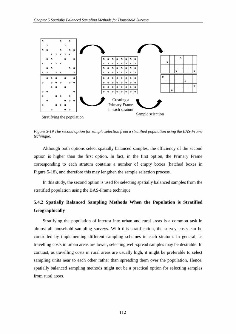
Chapter 5 Spatially Balanced Sampling Methods for Household Surveys
112
Figure 5-19 The second option for sample selection from a stratified population using the BAS-Frame
technique.
Although both options select spatially balanced samples, the efficiency of the second
option is higher than the first option. In fact, in the first option, the Primary Frame
corresponding to each stratum contains a number of empty boxes (hatched boxes in
Figure 5-18), and therefore this may lengthen the sample selection process.
In this study, the second option is used for selecting spatially balanced samples from the
stratified population using the BAS-Frame technique.
5.4.2 Spatially Balanced Sampling Methods When the Population is Stratified
Geographically
Stratifying the population of interest into urban and rural areas is a common task in
almost all household sampling surveys. With this stratification, the survey costs can be
controlled by implementing different sampling schemes in each stratum. In general, as
travelling costs in urban areas are lower, selecting well-spread samples may be desirable. In
contrast, as travelling costs in rural areas are usually high, it might be preferable to select
sampling units near to each other rather than spreading them over the population. Hence,
spatially balanced sampling methods might not be a practical option for selecting samples
from rural areas.
x x x
x x
x x x x x
x x x x x
x x x x
x x x x
x x x x
x x x x x
o o o o o
o o o o o o
o o o
o o o
o o o o
o o o o
o o o o
o o o
x x x x x x x x
x x x x x x x x
x x x x x x x x
x x x x x x x x
o o o o o o o o
o o o o o o o o
o o o o o o o o
o o o o o o o o
x
x
x x
o
o
o
o
Creating a
Primary Frame
in each stratumSample selection
Stratifying the population
Chapter 5 Spatially Balanced Sampling Methods for Household Surveys
113
This subsection aims to investigate the travelling costs in rural and urban areas when
sampling units are selected using spatially balanced sampling methods. For this, a simulation
study was conducted on meshblocks of Ashburton town in New Zealand. Meshblocks in this
town are categorized into five geographical levels: main urban, secondary urban, minor
urban, rural centre, and rural areas. Using this information, the “urban” stratum was generated
by combining main urban, secondary urban and minor urban meshblocks. The combination
of rural centre and rural area meshblocks, was considered as the “rural” stratum.
After defining rural and urban strata, two different spatially balanced sampling designs
(LPM and BAS-Frame technique) and a non-spatially balanced sampling method (SRS) were
employed to select sample meshblocks from each stratum by considering equal sampling
fractions. The sampling process was repeated 1000 times for three different sampling
fractions (10, 15 and 20%).
In the dataset, the only available information for modelling travel cost is the
geographical coordinates of the centre of meshblocks in the population frame. Therefore, by
assuming that travelling cost is affected only by travelling distance, the length of the path
among selected meshblocks is considered as an index to define the travelling costs for that
sample. The distance in this study was computed using the travelling salesperson problem
(TSP) (Hahsler & Hornik, 2007). TSP’s goal is to find the shortest path that visits each
sampled meshblock once and then returns to the starting meshblock.
After selecting 1000 samples, the average of the shortest distance for each sampling
method (��) was calculated using
�� = 1
1000 ∑ 𝑑𝑖
1000
𝑖=1
(5.5)
where 𝑑𝑖 is the shortest distance, which is determined with the help of TSP, for the 𝑖𝑡ℎ
iteration. The values 𝑑𝑖 and �� are expressed in kilometres (km).
The calculated values of �� for the evaluated sampling methods in the urban and rural
strata and for three different sampling fractions are shown in Table 5-9.
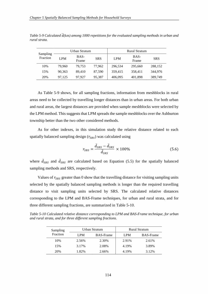
Chapter 5 Spatially Balanced Sampling Methods for Household Surveys
114
Table 5-9 Calculated ��(km) among 1000 repetitions for the evaluated sampling methods in urban and
rural strata.
Sampling
Fraction
Urban Stratum Rural Stratum
LPM BAS-
Frame SRS LPM
BAS-
Frame SRS
10% 79,960 79,753 77,962 296,534 295,660 288,152
15% 90,363 89,410 87,590 359,415 358,411 344,976
20% 97,125 97,927 95,387 406,095 401,898 389,749
As Table 5-9 shows, for all sampling fractions, information from meshblocks in rural
areas need to be collected by travelling longer distances than in urban areas. For both urban
and rural areas, the largest distances are provided when sample meshblocks were selected by
the LPM method. This suggests that LPM spreads the sample meshblocks over the Ashburton
township better than the two other considered methods.
As for other indexes, in this simulation study the relative distance related to each
spatially balanced sampling design (𝑟𝑆𝐵𝑆) was calculated using
𝑟𝑆𝐵𝑆 =��𝑆𝐵𝑆 − ��𝑆𝑅𝑆
��𝑆𝑅𝑆 × 100% (5.6)
where ��𝑆𝐵𝑆 and ��𝑆𝑅𝑆 are calculated based on Equation (5.5) for the spatially balanced
sampling methods and SRS, respectively.
Values of 𝑟𝑆𝐵𝑆 greater than 0 show that the travelling distance for visiting sampling units
selected by the spatially balanced sampling methods is longer than the required travelling
distance to visit sampling units selected by SRS. The calculated relative distances
corresponding to the LPM and BAS-Frame techniques, for urban and rural strata, and for
three different sampling fractions, are summarized in Table 5-10.
Table 5-10 Calculated relative distance corresponding to LPM and BAS-Frame technique, for urban
and rural strata, and for three different sampling fractions.
Sampling
Fraction
Urban Stratum Rural Stratum
LPM BAS-Frame LPM BAS-Frame
10% 2.56% 2.30% 2.91% 2.61%
15% 3.17% 2.08% 4.19% 3.89%
20% 1.82% 2.66% 4.19% 3.12%
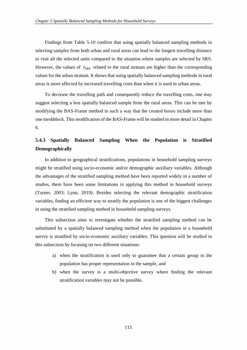
Chapter 5 Spatially Balanced Sampling Methods for Household Surveys
115
Findings from Table 5-10 confirm that using spatially balanced sampling methods in
selecting samples from both urban and rural areas can lead to the longest travelling distance
to visit all the selected units compared to the situation where samples are selected by SRS.
However, the values of 𝑟𝑆𝐵𝑆 related to the rural stratum are higher than the corresponding
values for the urban stratum. It shows that using spatially balanced sampling methods in rural
areas is more affected by increased travelling costs than when it is used in urban areas.
To decrease the travelling path and consequently reduce the travelling costs, one may
suggest selecting a less spatially balanced sample from the rural areas. This can be met by
modifying the BAS-Frame method in such a way that the created boxes include more than
one meshblock. This modification of the BAS-Frame will be studied in more detail in Chapter
6.
5.4.3 Spatially Balanced Sampling When the Population is Stratified
Demographically
In addition to geographical stratifications, populations in household sampling surveys
might be stratified using socio-economic and/or demographic auxiliary variables. Although
the advantages of the stratified sampling method have been reported widely in a number of
studies, there have been some limitations in applying this method in household surveys
(Turner, 2003; Lynn, 2019). Besides selecting the relevant demographic stratification
variables, finding an efficient way to stratify the population is one of the biggest challenges
in using the stratified sampling method in household sampling surveys.
This subsection aims to investigate whether the stratified sampling method can be
substituted by a spatially balanced sampling method when the population in a household
survey is stratified by socio-economic auxiliary variables. This question will be studied in
this subsection by focusing on two different situations:
a) when the stratification is used only to guarantee that a certain group in the
population has proper representation in the sample, and
b) when the survey is a multi-objective survey where finding the relevant
stratification variables may not be possible.
Chapter 5 Spatially Balanced Sampling Methods for Household Surveys
116
These two situations were studied through simulation on meshblocks of Christchurch
city. For simplicity, the population of meshblocks was stratified using only one stratification
variable.
Māori are deemed to be a group of high importance for most household sampling surveys
conducted by Stats NZ. Hence, Stats NZ tries to select an adequate representation of this
group in its household samples by targeting areas of high Māori population density. Usually
this is done by considering Māori population density as one of the stratification variables.
Here, to make the simulation studies more similar to the household sampling surveys of Stats
NZ, the density of the Māori population is considered as the stratification variable.
In this study, according to the proportion of Māori in meshblocks, the meshblocks in
Christchurch city are stratified into two strata:
1) stratum with high Māori population density (“high Māori”), and
2) stratum with low Māori population density (“low Māori”).
In this study, the high Māori stratum includes meshblocks that have more than 12 percent
Māori. In contrast, the proportion of Māori in meshblocks located in the low Māori stratum
is less than 12 percent. The total number of meshblocks in Christchurch city that are located
in the high Māori stratum is almost 4 times greater than the number of meshblocks located in
the low Māori stratum.
The details of the simulation studies related to each of the two situations mentioned
above are explained next.
Situation (a): when the stratification is used only to guarantee that a certain group
in the population has proper representation in the sample
In some practical cases, the stratification process is done only to ensure that all target
groups – especially those that represent a small proportion of the population – are represented
in the sample appropriately. In these situations, the stratification is not aimed at providing
separate estimates for these groups. Chapter 4 of this thesis showed that in cases of continuous
populations, the BAS method can perform as well as the stratified sampling method with
proportional allocation; in other words, the population does not need to be stratified explicitly.
As explained before, this is because the number of sampling units selected by BAS from a
specific part of a continuous population is proportional to the area of that part.
Chapter 5 Spatially Balanced Sampling Methods for Household Surveys
117
The simulation study in this subsection aims to understand whether the BAS-Frame
method can be used as an alternative method to the stratified sampling method with
proportional allocation for selecting samples from a stratified discrete population.
In the simulation study, 1000 samples of different sizes (1, 2, 3, 4, and 5% of the total
number of meshblocks) were selected from the meshblocks of Christchurch city without
attention to the boundaries of the defined strata (high Māori and low Māori). Samples were
selected using two spatially balanced sampling methods (LPM and BAS-Frame) and a non-
spatially balanced sampling method (SRS). For each selected sample the numbers of
meshblocks located in the low Māori stratum and high Māori stratum were counted. Let
𝑚ℎ𝑖 (ℎ ∈ {𝑙𝑜𝑤 𝑀��𝑜𝑟𝑖, ℎ𝑖𝑔ℎ 𝑀��𝑜𝑟𝑖}, 𝑖 = 1, … , 1000) be the number of selected
meshblocks within stratum ℎ at the 𝑖𝑡ℎ iteration.
Using the stratified sampling method with proportional allocation ensures that the
number of selected meshblocks in the high Māori stratum was almost 4 times greater than the
number of selected meshblocks in the low Māori stratum. Therefore, comparing the values of
𝑚ℎ𝑖 with the expected value according to the proportional allocation will reveal to what extent
the performance of the evaluated designs is close to the performance of the proportional
stratified sampling method. The average values and variance of 𝑚ℎ𝑖 among all iterations for
all evaluated designs and all sample sizes are shown in Table 5-11. The numbers of allocated
meshblocks to strata according to the stratified sampling method with proportional allocation
are in bold in Table 5-11.
As seen in Table 5-11, for all the sample sizes, the average number of selected
meshblocks (𝑚ℎ𝑖) in each stratum obtained by spatially balanced sampling methods
satisfactorily matches the expected values associated with a proportional stratified sampling
method. This means that the samples selected by the spatially balanced sampling methods
consist of meshblocks with different Māori population density. The results confirm that
implementing a spatially balanced sampling method in irregular discrete populations can
perform as well as proportional stratified sampling.
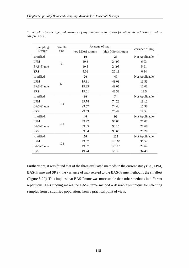
Chapter 5 Spatially Balanced Sampling Methods for Household Surveys
118
Table 5-11 The average and variance of 𝑚ℎ𝑖 among all iterations for all evaluated designs and all
sample sizes.
Sampling
Design
Sample
size
Average of 𝑚ℎ𝑖 Variance of 𝑚ℎ𝑖
low Māori stratum high Māori stratum
stratified
35
10 25 Not Applicable
LPM 10.3 24.97 6.03
BAS-Frame 10.5 24.95 5.91
SRS 9.01 26.19 6.94
stratified
69
20 49 Not Applicable
LPM 19.91 49.09 13.53
BAS-Frame 19.85 49.05 10.01
SRS 19.01 48.39 13.5
stratified
104
30 74 Not Applicable
LPM 29.78 74.22 18.12
BAS-Frame 29.57 74.43 15.98
SRS 29.53 74.47 19.54
stratified
138
40 98 Not Applicable
LPM 39.92 98.08 25.02
BAS-Frame 39.85 98.15 20.68
SRS 39.34 98.66 25.29
stratified
173
50 123 Not Applicable
LPM 49.67 123.63 31.52
BAS-Frame 49.87 123.13 25.64
SRS 49.24 123.76 34.49
Furthermore, it was found that of the three evaluated methods in the current study (i.e., LPM,
BAS-Frame and SRS), the variance of 𝑚ℎ𝑖 related to the BAS-Frame method is the smallest
(Figure 5-20). This implies that BAS-Frame was more stable than other methods in different
repetitions. This finding makes the BAS-Frame method a desirable technique for selecting
samples from a stratified population, from a practical point of view.
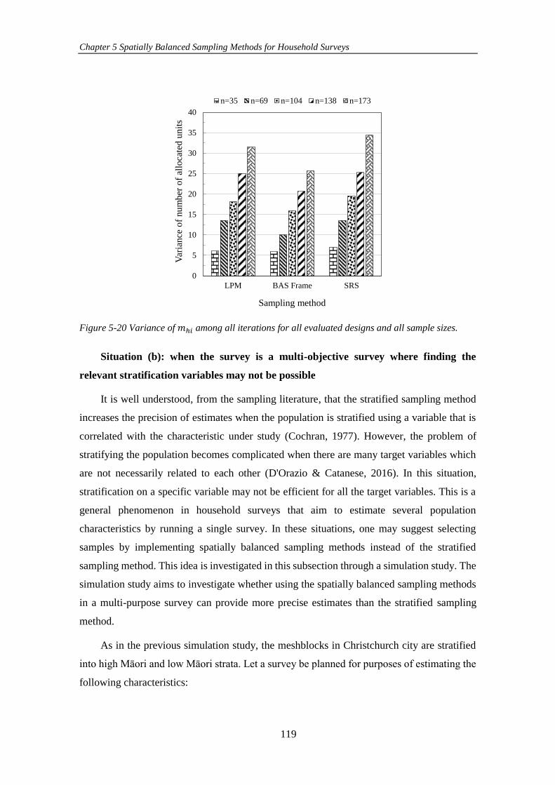
Chapter 5 Spatially Balanced Sampling Methods for Household Surveys
119
Figure 5-20 Variance of 𝑚ℎ𝑖 among all iterations for all evaluated designs and all sample sizes.
Situation (b): when the survey is a multi-objective survey where finding the
relevant stratification variables may not be possible
It is well understood, from the sampling literature, that the stratified sampling method
increases the precision of estimates when the population is stratified using a variable that is
correlated with the characteristic under study (Cochran, 1977). However, the problem of
stratifying the population becomes complicated when there are many target variables which
are not necessarily related to each other (D'Orazio & Catanese, 2016). In this situation,
stratification on a specific variable may not be efficient for all the target variables. This is a
general phenomenon in household surveys that aim to estimate several population
characteristics by running a single survey. In these situations, one may suggest selecting
samples by implementing spatially balanced sampling methods instead of the stratified
sampling method. This idea is investigated in this subsection through a simulation study. The
simulation study aims to investigate whether using the spatially balanced sampling methods
in a multi-purpose survey can provide more precise estimates than the stratified sampling
method.
As in the previous simulation study, the meshblocks in Christchurch city are stratified
into high Māori and low Māori strata. Let a survey be planned for purposes of estimating the
following characteristics:
0
5
10
15
20
25
30
35
40
LPM BAS Frame SRS
Var
ian
ce o
f n
um
ber
of
allo
cate
d u
nit
s
Sampling method
n=35 n=69 n=104 n=138 n=173
Chapter 5 Spatially Balanced Sampling Methods for Household Surveys
120
total number of people who bike to work,
total number of people who have a partner,
total number of females with no alive born children,
total number of people who can speak te reo Māori (the Māori language) , and
total number of people who are involved in unpaid household work.
Of the five considered target variables, it could be assumed that “people who can speak
te reo Māori” is the only variable that might have a correlation with the stratification variable
(high/low Māori). On the basis of the available dataset, there is a positive correlation between
the “people who can speak te reo Māori” and the stratification variable (i.e., approximately
11%). The other variables do not have any correlation with the stratification variable.
Sample meshblocks in this study were selected using SRS, LPM and BAS-Frame
methods separately in each created stratum. Also, LPM and BAS-Frame were used to select
spatial samples without attention to the boundaries of the strata. The sample selection was
repeated 1000 times and for five different sample sizes (1, 2, 3, 4, and 5% of the total number
of meshblocks). For simplicity, the same sampling fraction was used in each stratum.
After selecting samples, the variance of the HT estimator for estimating the
characteristics of interest was estimated for each evaluated sampling method. In order to
compare the evaluated designs, the ratio of variance related to each spatially balanced
sampling design was calculated by dividing the simulated variance of that spatial design by
the simulated variance of the stratified SRS.
Ratio of Variance = Variance of spatially balanced sampling design
variance of stratified SRS. (5.7)
The ratio of variances related to each characteristic and for all sample sizes are reported
in Table 5-12. Trends of ratio of variances related to each target variable among the different
sample sizes are shown in Figure 5-21.
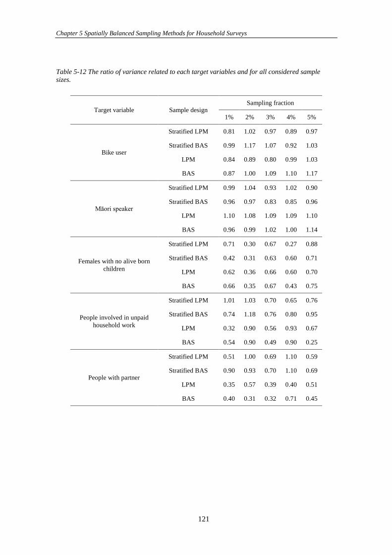
Chapter 5 Spatially Balanced Sampling Methods for Household Surveys
121
Table 5-12 The ratio of variance related to each target variables and for all considered sample sizes.
Target variable Sample design Sampling fraction
1% 2% 3% 4% 5%
Bike user
Stratified LPM 0.81 1.02 0.97 0.89 0.97
Stratified BAS 0.99 1.17 1.07 0.92 1.03
LPM 0.84 0.89 0.80 0.99 1.03
BAS 0.87 1.00 1.09 1.10 1.17
Māori speaker
Stratified LPM 0.99 1.04 0.93 1.02 0.90
Stratified BAS 0.96 0.97 0.83 0.85 0.96
LPM 1.10 1.08 1.09 1.09 1.10
BAS 0.96 0.99 1.02 1.00 1.14
Females with no alive born
children
Stratified LPM 0.71 0.30 0.67 0.27 0.88
Stratified BAS 0.42 0.31 0.63 0.60 0.71
LPM 0.62 0.36 0.66 0.60 0.70
BAS 0.66 0.35 0.67 0.43 0.75
People involved in unpaid
household work
Stratified LPM 1.01 1.03 0.70 0.65 0.76
Stratified BAS 0.74 1.18 0.76 0.80 0.95
LPM 0.32 0.90 0.56 0.93 0.67
BAS 0.54 0.90 0.49 0.90 0.25
People with partner
Stratified LPM 0.51 1.00 0.69 1.10 0.59
Stratified BAS 0.90 0.93 0.70 1.10 0.69
LPM 0.35 0.57 0.39 0.40 0.51
BAS 0.40 0.31 0.32 0.71 0.45
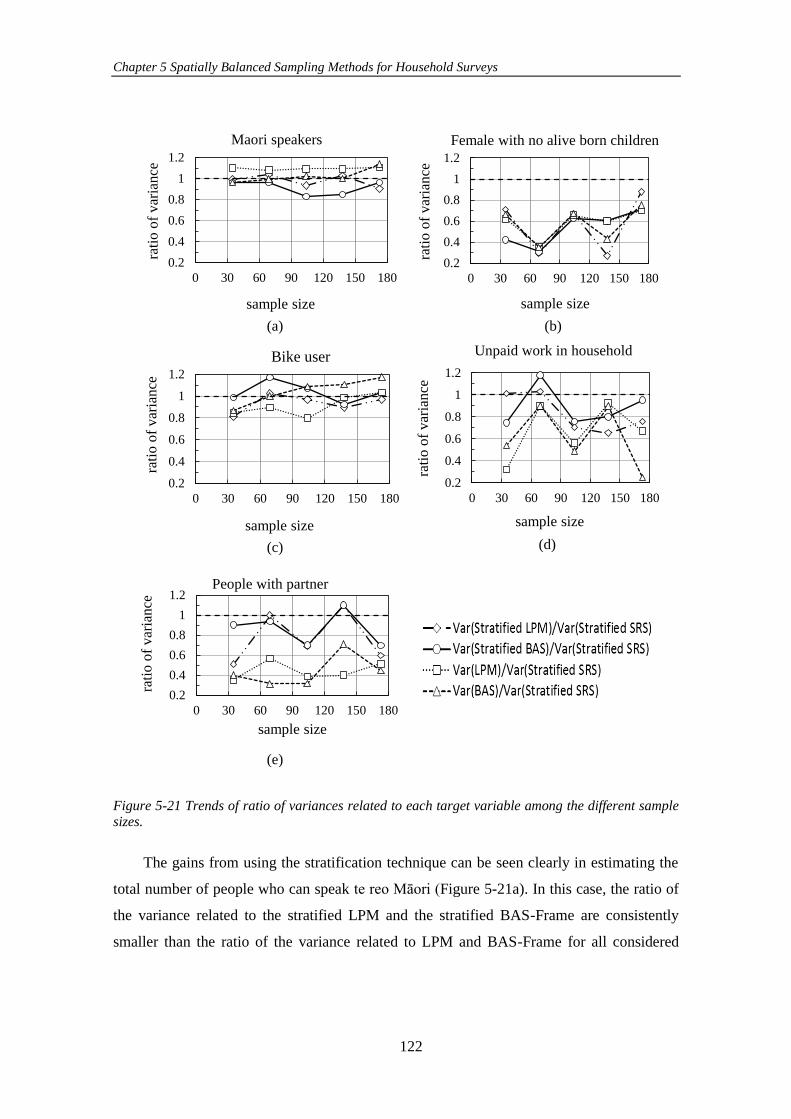
Chapter 5 Spatially Balanced Sampling Methods for Household Surveys
122
Figure 5-21 Trends of ratio of variances related to each target variable among the different sample sizes.
The gains from using the stratification technique can be seen clearly in estimating the
total number of people who can speak te reo Māori (Figure 5-21a). In this case, the ratio of
the variance related to the stratified LPM and the stratified BAS-Frame are consistently
smaller than the ratio of the variance related to LPM and BAS-Frame for all considered
0.2
0.4
0.6
0.8
1
1.2
0 30 60 90 120 150 180
rati
o o
f v
aria
nce
sample size
Maori speakers
0.2
0.4
0.6
0.8
1
1.2
0 30 60 90 120 150 180
rati
o o
f v
aria
nce
sample size
Bike user
(a) (b)
(c) (d)
0.2
0.4
0.6
0.8
1
1.2
0 30 60 90 120 150 180
rati
o o
f v
aria
nce
sample size
Female with no alive born children
0.2
0.4
0.6
0.8
1
1.2
0 30 60 90 120 150 180
rati
o o
f v
aria
nce
sample size
Unpaid work in household
0.2
0.4
0.6
0.8
1
1.2
0 30 60 90 120 150 180
rati
o o
f v
aria
nce
sample size
People with partner
(e)
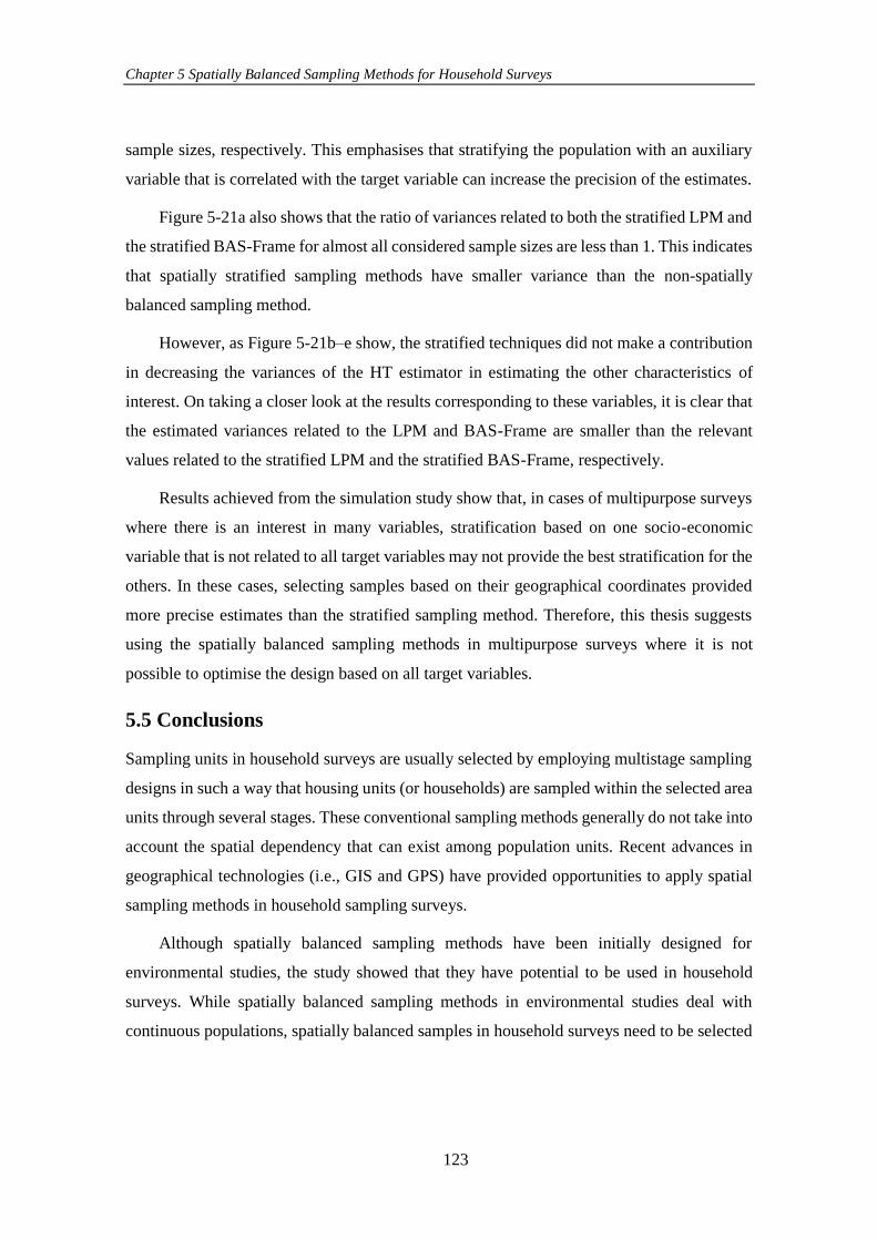
Chapter 5 Spatially Balanced Sampling Methods for Household Surveys
123
sample sizes, respectively. This emphasises that stratifying the population with an auxiliary
variable that is correlated with the target variable can increase the precision of the estimates.
Figure 5-21a also shows that the ratio of variances related to both the stratified LPM and
the stratified BAS-Frame for almost all considered sample sizes are less than 1. This indicates
that spatially stratified sampling methods have smaller variance than the non-spatially
balanced sampling method.
However, as Figure 5-21b–e show, the stratified techniques did not make a contribution
in decreasing the variances of the HT estimator in estimating the other characteristics of
interest. On taking a closer look at the results corresponding to these variables, it is clear that
the estimated variances related to the LPM and BAS-Frame are smaller than the relevant
values related to the stratified LPM and the stratified BAS-Frame, respectively.
Results achieved from the simulation study show that, in cases of multipurpose surveys
where there is an interest in many variables, stratification based on one socio-economic
variable that is not related to all target variables may not provide the best stratification for the
others. In these cases, selecting samples based on their geographical coordinates provided
more precise estimates than the stratified sampling method. Therefore, this thesis suggests
using the spatially balanced sampling methods in multipurpose surveys where it is not
possible to optimise the design based on all target variables.
5.5 Conclusions
Sampling units in household surveys are usually selected by employing multistage sampling
designs in such a way that housing units (or households) are sampled within the selected area
units through several stages. These conventional sampling methods generally do not take into
account the spatial dependency that can exist among population units. Recent advances in
geographical technologies (i.e., GIS and GPS) have provided opportunities to apply spatial
sampling methods in household sampling surveys.
Although spatially balanced sampling methods have been initially designed for
environmental studies, the study showed that they have potential to be used in household
surveys. While spatially balanced sampling methods in environmental studies deal with
continuous populations, spatially balanced samples in household surveys need to be selected
Chapter 5 Spatially Balanced Sampling Methods for Household Surveys
124
from target populations that typically consist of a finite number of discrete units. Thus, in this
chapter, a new modification of the BAS method, the BAS-Frame method, was developed.
Results from simulations showed that the BAS-Frame method is able to select spatially
balanced samples as well as other spatially balanced sampling methods.
In the second part of this chapter, the BAS-Frame method along with spatially balanced
sampling methods were examined in the process of selecting samples from a list of
meshblocks in the region of Canterbury, New Zealand. The outcomes indicated that spatially
balanced sampling methods provided more precise estimates of the population characteristics
when compared to the SRS method in spite of relatively poor spatial autocorrelation for the
considered response variables. It was found that LPM has the best performance among all the
methods evaluated in this study.
The third part of the chapter investigated the application of the BAS-Frame method in
populations that are stratified either geographically or demographically. In household
surveys, a common geographical stratification variable is urban/rural area. In order to
investigate the undesirable effect of spatially balanced sampling on the survey cost in each
urban and rural area, a simulation was performed on a population that was stratified into rural
and urban strata. Results of the simulation study confirmed that in comparison to SRS, using
the spatially balanced sampling in a rural stratum may increase the travel costs, while travel
cost increase is not marked in the urban stratum.
Regarding the use of geographic variables in the stratification process, this chapter
focused on two different situations: when the stratification is used only to guarantee that
sampling units are spread evenly over the population and when a population needs to be
stratified for running a multi-objective survey. Findings derived from the simulation studies
showed that, for the first situation, and in cases where the same sampling fraction is used in
all strata, it is not necessary to stratify the population explicitly. In these cases, a BAS-Frame
technique can be used as an alternative method to the stratified sampling method with
proportional allocation. Finding a suitable stratification variable that is related to all target
variables is one difficulty in using the stratified sampling in multi-objective surveys. One
suggestion to address this difficulty is using spatially balanced sampling methods. This
suggestion was investigated through a simulation study. Results of the simulation study
showed that the spatially balanced sampling methods provided more precise estimates than
Chapter 5 Spatially Balanced Sampling Methods for Household Surveys
125
the stratified sampling method when the survey is a multi-objectives survey and finding a
relevant stratification variable is not possible.
5.6 References
Agrawal, R., & Srikant, R. (2000). Privacy-preserving data mining. ACM Sigmod Record, 29(2),
439-450.
Alves, S. (2012). The patterns of unemployment and the geography of social housing. World
Academy of Science, Engineering and Technology, 71, 759-767.
Bast, H., & Hert, S. (2000). The area partitioning problem. Paper presented at the 12th Canadian
Conference on Computational Geometry, Fredericton, New Brunswick.
Carlsson, J. G., Armbruster, B., & Ye, Y. (2010). Finding equitable convex partitions of points in
a polygon efficiently. ACM Transactions on Algorithms (TALG), 6(4), 72.
Cochran, W. G. (1977). Sampling Techniques: 3d Ed: Wiley.
Cuberes, D., & Roberts, J. (2015). Household location and income: a spatial analysis for British
cities. The Sheffield Economic Research Paper Series (SERPS), 201502(022).
D'Orazio, M., & Catanese, E. (2016). A New Approach for Multipurpose Stratification in
Agriculture Surveys. Paper presented at the Fifth International Conference of
Establishment Surveys, Geneve.
Geuder, J. (1984). Paper stratification in SRS area sampling frames: US Department of
Agriculture, Statistical Reporting Service, Statistical Research Division.
Grafström, A., Lundström, N. L., & Schelin, L. (2012). Spatially balanced sampling through the
pivotal method. Biometrics, 68(2), 514-520.
Gregoire, T. G., & Valentine, H. T. (2007). Sampling strategies for natural resources and the
environment: CRC Press.
Hahsler, M., & Hornik, K. (2007). TSP-Infrastructure for the traveling salesperson problem.
Journal of Statistical Software, 23(2), 1-21.
Harrison Jr, D., & Rubinfeld, D. L. (1978). Hedonic housing prices and the demand for clean air.
Journal of Environmental Economics and Management, 5(1), 81-102.
Kalogirou, S., & Hatzichristos, T. (2007). A spatial modelling framework for income estimation.
Spatial Economic Analysis, 2(3), 297-316.
Kantar, Y. M., & Aktaş, S. G. (2016). Spatial Correlation Analysis of Unemployment Rates in
Turkey. Journal of Eastern Europe Research in Business and Economics, 1-9.
Kish, L. (1965). Survey sampling. New York: John Wiley and Sons.
Lynn, P. (2019). The advantage and disadvantage of implicitly stratified sampling. MDA:
methods, data, analyses, 13(2), 14.
O'Campo, P., Wheaton, B., Nisenbaum, R., Glazier, R. H., Dunn, J. R., & Chambers, C. (2015).
The neighbourhood effects on health and well-being (NEHW) study. Health & place, 31,
65-74.
Olea, R. A. (1984). Sampling design optimization for spatial functions. Journal of the
International Association for Mathematical Geology, 16(4), 369-392.
Chapter 5 Spatially Balanced Sampling Methods for Household Surveys
126
Pfeffermann, D., & Rao, C. R. (2009). Sample surveys: Design, methods and applications:
Elsevier.
Robertson, B., Brown, J., McDonald, T., & Jaksons, P. (2013). BAS: balanced acceptance
sampling of natural resources. Biometrics, 69(3), 776-784.
Robertson, B., McDonald, T., Price, C., & Brown, J. (2017). A modification of balanced
acceptance sampling. Statistics & Probability Letters, 129, 107-112.
Stats NZ. (2013a). Retrieved from https://www.stats.govt.nz/large-datasets/csv-files-for-
download/
Stats NZ. (2013b). Meshblock definition. Retrieved from
http://archive.stats.govt.nz/methods/classifications-and-standards/classification-related-
stats-standards/meshblock/definition.aspx
Stevens, D., & Olsen, A. (2004). Spatially balanced sampling of natural resources. Journal of the
American Statistical Association, 99(465), 262-278.
Turner, A. G. (2003). Sampling strategies. Handbook on designing of household sample surveys.
Geneva: United Nations Statistics Division.
127
Properties of Sampling Frames for Spatial
Sampling in Household Surveys
6.1 Introduction
To conduct a probability sample a list of target units should be available from which the
samples are drawn. Such a list is called a sampling frame (Särndal et al., 2003). In ideal
situations, when sampling frames are available, “area frame” and “list frame” are the two
most common types of frames that are used to design a household survey (Turner, 2003).
These frames are developed usually by national statistical agencies, based on the information
obtained from censuses. Therefore, these frames are supposed to be accurate and reliable at
the date of conducting the censuses.
However, as time goes on, getting an up-to-date and reliable version of area frames and
list frames, especially in regions where rapid changes are frequent, is very difficult. In these
situations, alternative sampling frames (i.e., lists of residential postal addresses or lists of
telephone numbers) and consequently different sampling approaches should be considered
for household surveys.
Furthermore, sometimes the household surveys need to be conducted in a non-ideal
situation where often the sampling frames are not available (e.g., designing a survey after a
disaster or selecting a sample from poorly resourced settings). The absence of a well-defined
sampling frame in non-ideal situations is a great challenge for survey statisticians and
motivates them to use new technologies (Google Earth imagery, GIS, etc.) and new sampling
schemes.
This chapter aims to investigate the feasibility of applying spatially balanced sampling
methods for selecting spatial samples in the three different situations mentioned above (in the
presence of an area frame or a list frame in ideal situations, in the presence of a list of
residential postal addresses, and in non-ideal situations where there is lack of reliable
sampling frame). The application of spatially balanced sampling methods for selecting
samples in a two-stage cluster sampling design – which is a common household sampling
design– will be studied in the next section. In that section, the precision of spatially balanced
Chapter 6 Properties of Sampling Frames for Spatial Sampling in Household Surveys
128
sampling methods in selecting primary sampling units from an area frame in the first stage of
a two-stage cluster sampling design will be compared with the precision of a probability
proportional to size (PPS) without replacement sampling method. Then, for sampling in the
second stage, the precision of the spatially balanced sampling methods will be compared with
the precision of systematic sampling for selecting ultimate units from a list frame.
The third section of this chapter describes how spatially balanced sampling methods can
be used to select sample households directly from a list of addresses of households. A
modification of the BAS-Frame technique for conducting a spatial single-stage and a spatial
two-stage cluster sample will be introduced.
Finally, the fourth section will explain the application of the BAS method for selecting
samples in non-ideal situations.
6.2 Spatially Balanced Sampling Methods in Conducting a Two-Stage
Cluster Sampling
6.2.1 Stage 1 – Selecting Sample Area Units in the Presence of an Area Frame
An area frame in a household survey is usually made up of geographical units of a country
that are arranged hierarchically. This frame typically includes some features such as cities,
districts, villages in rural regions and blocks in urban regions. Each feature in an area frame
is assigned a unique code. Geographical units in an ideal area frame cover the entire area of
the target population and each unit has well-defined boundaries. A list of meshblocks in
Christchurch is an example of an area frame.
As explained in Chapter 2, area frames are usually used at the first stage of the sample
selection process in household surveys. In classical household sampling techniques, sample
area units are often selected from area frames using a PPS sampling method. However, this
sampling method does not guarantee that the selected area units are well spread over the
population.
With the increasing availability of geographical information (e.g., online maps, and
satellite imagery), the sampling selection process in the first stage of a household sampling
survey can be enhanced by employing spatially balanced sampling methods. In this
subsection, the effect of using spatially balanced sampling methods on increasing the
representativeness of area samples was investigated through conducting a simulation study
Chapter 6 Properties of Sampling Frames for Spatial Sampling in Household Surveys
129
on Christchurch meshblocks. The available area frame of meshblocks contains a list of the
meshblocks’ unique codes as well as the geographical coordinates of the geometric centre of
each meshblock and some attributes related to each meshblock. The geographical positions
of the centre of the meshblocks are shown in Figure 5-14. In this thesis, the geometric centre
of meshblocks were calculated using “sp” package in R (R Core Team, 2017).
In the simulation study, sample area units (meshblocks) were selected using five
different sampling methods:
1) PPS systematic (PPS-SYS) sampling without replacement where meshblocks
arranged by their unique codes,
2) PPS-SYS sampling without replacement where meshblocks arranged firstly by
their longitude and then by their latitude,
3) Spatially balanced sampling methods (LPM, BAS-Frame with adding random
points and GRTS) with unequal sample inclusion probability,
4) Balanced sampling (CUBE method), and
5) Conditional Poisson (CP) sampling.
PPS-SYS sampling selects samples by using systematic random sampling with
probability proportional to size. In this method sampling units are selected at a fixed selection
interval throughout the sampling frame after selection of a random start. The systematic
selection interval is the ratio of the total size to the sample size (𝑀 𝑛⁄ ). If the size of the 𝑖𝑡ℎ
unit (𝑀𝑖) is greater than the selection interval, the 𝑖𝑡ℎ unit might be selected more than once.
To avoid any duplications in the sample, the size of the 𝑖𝑡ℎ unit (𝑀𝑖) is required to be less
than 𝑀 𝑛⁄ .
Poisson sampling is a sampling design for selecting samples with unequal inclusion
probabilities. For Poisson sampling, each unit is selected according to an independent
Bernoulli trial. This will provide a random sample size. CP is a special case of Poisson
sampling introduced by Hajek and Dupac (1981) where the condition of selecting a sample
with a fixed sample size is added. To achieve a fixed sample size, it is possible to generate
Poisson samples and accept the sample only if it has the required sample size. In this study,
CP is used as a benchmark method to compare the unequal probability sampling designs.
As previously discussed in Chapter 5, for selecting samples with equal inclusion
probability by means of BAS-Frame, the process of creating a primary frame can be done
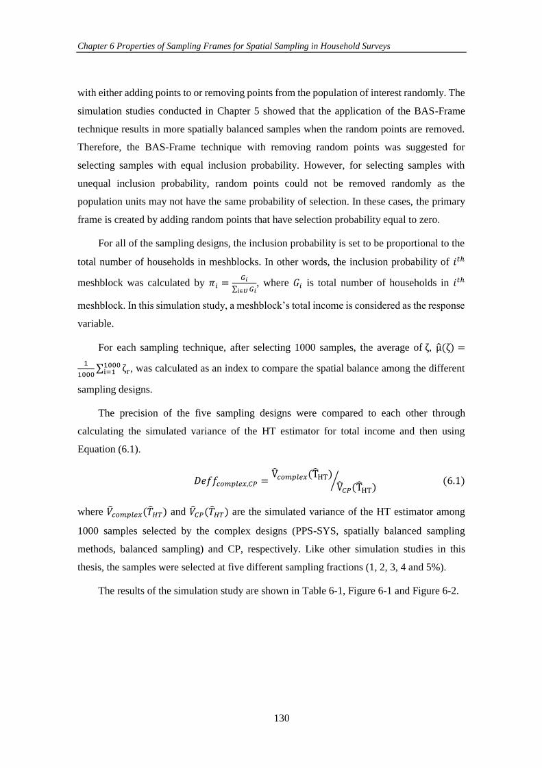
Chapter 6 Properties of Sampling Frames for Spatial Sampling in Household Surveys
130
with either adding points to or removing points from the population of interest randomly. The
simulation studies conducted in Chapter 5 showed that the application of the BAS-Frame
technique results in more spatially balanced samples when the random points are removed.
Therefore, the BAS-Frame technique with removing random points was suggested for
selecting samples with equal inclusion probability. However, for selecting samples with
unequal inclusion probability, random points could not be removed randomly as the
population units may not have the same probability of selection. In these cases, the primary
frame is created by adding random points that have selection probability equal to zero.
For all of the sampling designs, the inclusion probability is set to be proportional to the
total number of households in meshblocks. In other words, the inclusion probability of 𝑖𝑡ℎ
meshblock was calculated by 𝜋𝑖 =𝐺𝑖
∑ 𝐺𝑖𝑖∈𝑈, where 𝐺𝑖 is total number of households in 𝑖𝑡ℎ
meshblock. In this simulation study, a meshblock’s total income is considered as the response
variable.
For each sampling technique, after selecting 1000 samples, the average of ζ, μ(ζ) =
1
1000∑ ζr1000i=1 , was calculated as an index to compare the spatial balance among the different
sampling designs.
The precision of the five sampling designs were compared to each other through
calculating the simulated variance of the HT estimator for total income and then using
Equation (6.1).
𝐷𝑒𝑓𝑓𝑐𝑜𝑚𝑝𝑙𝑒𝑥,𝐶𝑃 =V𝑐𝑜𝑚𝑝𝑙𝑒𝑥(THT)
V𝐶𝑃(THT)⁄ (6.1)
where ��𝑐𝑜𝑚𝑝𝑙𝑒𝑥(��𝐻𝑇) and ��𝐶𝑃(��𝐻𝑇) are the simulated variance of the HT estimator among
1000 samples selected by the complex designs (PPS-SYS, spatially balanced sampling
methods, balanced sampling) and CP, respectively. Like other simulation studies in this
thesis, the samples were selected at five different sampling fractions (1, 2, 3, 4 and 5%).
The results of the simulation study are shown in Table 6-1, Figure 6-1 and Figure 6-2.
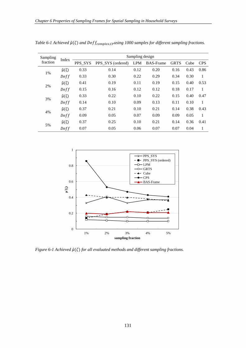
Chapter 6 Properties of Sampling Frames for Spatial Sampling in Household Surveys
131
Table 6-1 Achieved ��(𝜁) and 𝐷𝑒𝑓𝑓𝑐𝑜𝑚𝑝𝑙𝑒𝑥,𝐶𝑃using 1000 samples for different sampling fractions.
Sampling
fraction Index
Sampling design
PPS_SYS PPS_SYS (ordered) LPM BAS-Frame GRTS Cube CPS
1% μ(ζ) 0.33 0.14 0.12 0.20 0.16 0.43 0.86
𝐷𝑒𝑓𝑓 0.33 0.30 0.22 0.29 0.34 0.30 1
2% μ(ζ) 0.41 0.19 0.11 0.19 0.15 0.40 0.53
𝐷𝑒𝑓𝑓 0.15 0.16 0.12 0.12 0.18 0.17 1
3% μ(ζ) 0.33 0.22 0.10 0.22 0.15 0.40 0.47
𝐷𝑒𝑓𝑓 0.14 0.10 0.09 0.13 0.11 0.10 1
4% μ(ζ) 0.37 0.21 0.10 0.21 0.14 0.38 0.43
𝐷𝑒𝑓𝑓 0.09 0.05 0.07 0.09 0.09 0.05 1
5% μ(ζ) 0.37 0.25 0.10 0.21 0.14 0.36 0.41
𝐷𝑒𝑓𝑓 0.07 0.05 0.06 0.07 0.07 0.04 1
Figure 6-1 Achieved ��(𝜁) for all evaluated methods and different sampling fractions.
0
0.2
0.4
0.6
0.8
1
1% 2% 3% 4% 5%
μ(ζ)
sampling fraction
PPS_SYS
PPS_SYS (ordered)
LPM
GRTS
Cube
CPS
BAS-Frame
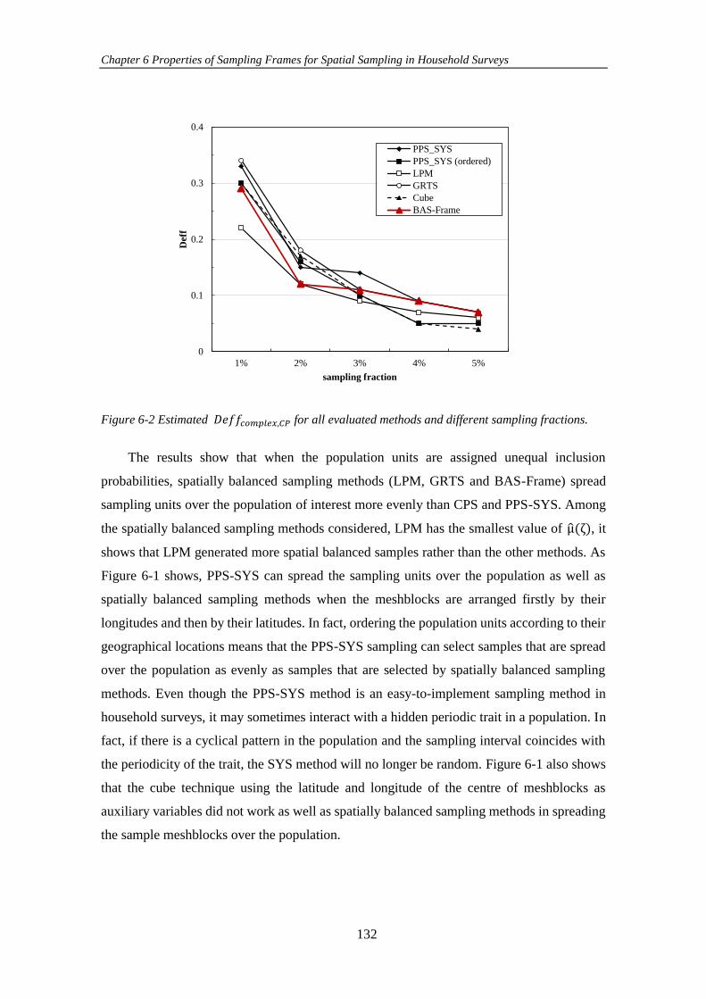
Chapter 6 Properties of Sampling Frames for Spatial Sampling in Household Surveys
132
Figure 6-2 Estimated 𝐷𝑒𝑓𝑓𝑐𝑜𝑚𝑝𝑙𝑒𝑥,𝐶𝑃 for all evaluated methods and different sampling fractions.
The results show that when the population units are assigned unequal inclusion
probabilities, spatially balanced sampling methods (LPM, GRTS and BAS-Frame) spread
sampling units over the population of interest more evenly than CPS and PPS-SYS. Among
the spatially balanced sampling methods considered, LPM has the smallest value of μ(ζ), it
shows that LPM generated more spatial balanced samples rather than the other methods. As
Figure 6-1 shows, PPS-SYS can spread the sampling units over the population as well as
spatially balanced sampling methods when the meshblocks are arranged firstly by their
longitudes and then by their latitudes. In fact, ordering the population units according to their
geographical locations means that the PPS-SYS sampling can select samples that are spread
over the population as evenly as samples that are selected by spatially balanced sampling
methods. Even though the PPS-SYS method is an easy-to-implement sampling method in
household surveys, it may sometimes interact with a hidden periodic trait in a population. In
fact, if there is a cyclical pattern in the population and the sampling interval coincides with
the periodicity of the trait, the SYS method will no longer be random. Figure 6-1 also shows
that the cube technique using the latitude and longitude of the centre of meshblocks as
auxiliary variables did not work as well as spatially balanced sampling methods in spreading
the sample meshblocks over the population.
0
0.1
0.2
0.3
0.4
1% 2% 3% 4% 5%
Def
f
sampling fraction
PPS_SYS
PPS_SYS (ordered)
LPM
GRTS
Cube
BAS-Frame
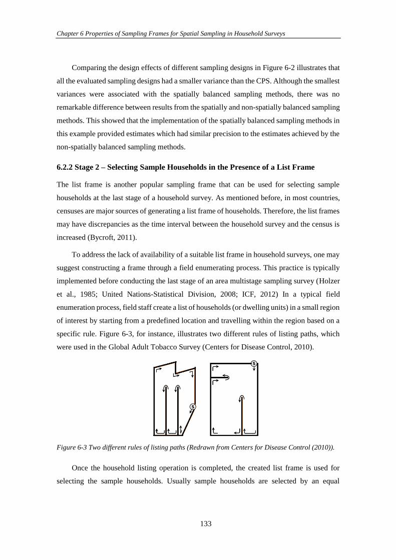
Chapter 6 Properties of Sampling Frames for Spatial Sampling in Household Surveys
133
Comparing the design effects of different sampling designs in Figure 6-2 illustrates that
all the evaluated sampling designs had a smaller variance than the CPS. Although the smallest
variances were associated with the spatially balanced sampling methods, there was no
remarkable difference between results from the spatially and non-spatially balanced sampling
methods. This showed that the implementation of the spatially balanced sampling methods in
this example provided estimates which had similar precision to the estimates achieved by the
non-spatially balanced sampling methods.
6.2.2 Stage 2 – Selecting Sample Households in the Presence of a List Frame
The list frame is another popular sampling frame that can be used for selecting sample
households at the last stage of a household survey. As mentioned before, in most countries,
censuses are major sources of generating a list frame of households. Therefore, the list frames
may have discrepancies as the time interval between the household survey and the census is
increased (Bycroft, 2011).
To address the lack of availability of a suitable list frame in household surveys, one may
suggest constructing a frame through a field enumerating process. This practice is typically
implemented before conducting the last stage of an area multistage sampling survey (Holzer
et al., 1985; United Nations-Statistical Division, 2008; ICF, 2012) In a typical field
enumeration process, field staff create a list of households (or dwelling units) in a small region
of interest by starting from a predefined location and travelling within the region based on a
specific rule. Figure 6-3, for instance, illustrates two different rules of listing paths, which
were used in the Global Adult Tobacco Survey (Centers for Disease Control, 2010).
Figure 6-3 Two different rules of listing paths (Redrawn from Centers for Disease Control (2010)).
Once the household listing operation is completed, the created list frame is used for
selecting the sample households. Usually sample households are selected by an equal
Chapter 6 Properties of Sampling Frames for Spatial Sampling in Household Surveys
134
probability systematic sampling method. In fact, using the systematic sampling method at the
last stage of a household survey aims to spread the sampling households over the region of
the target population and prevent the selection of a collection of neighbouring households.
The use of GPS to record the geographical coordinates of households in the listing
operation will provide some geographical visualization of the population units. Consequently,
in addition to systematic sampling, other spatially balanced sampling methods can be used to
select a well-spread sample.
In the previous chapters, the results of the simulation studies of applying spatially
balanced sampling methods for selecting samples showed that the LPM and the BAS-Frame
(with the random point removal option) are preferred to the other spatially balanced sampling
methods in spreading out the sampling units over the population. The findings provided
evidence that the LPM method and the BAS-Frame method can be used as alternatives to
systematic sampling at the last stage of a sampling household survey.
Of note, however, is the inability of the LPM and BAS-Frame methods to select sample
households at the time of generating a list frame. In fact, using a systematic sampling method
at the last stage of a household sampling survey does mean that it is possible to extract sample
households at the same time as providing a list of households. This is a practical advantage
of systematic sampling when compared with LPM and BAS-Frame, because for these two
methods the list frame need to be implemented after completing the field listing process.
Therefore, in practical cases where the household listing and sample selection process
need to be done at the same time, systematic sampling might be a good solution. In cases
where extracting the geographical coordinates of households without running a listing process
is possible, using the LPM method is recommended as it is more effective in spreading the
sample when the population size is fairly small.
6.3 Spatially Balanced Sampling Methods in the Presence of a List of
Household Registry
In the first section of this chapter, the possibility of using spatially balanced sampling
methods in the classical sampling designs currently used in household surveys has been
studied. This section investigates how the spatially balanced sampling methods can be
implemented with new forms of sampling frames.
Chapter 6 Properties of Sampling Frames for Spatial Sampling in Household Surveys
135
The high cost of household listing and data collection in a face-to-face interviewing
technique (an in-person survey), which has historically been used in household surveys, has
motivated statisticians to use alternative sampling frame and/or interviewing techniques (Link
et al., 2008). A telephone sampling survey based on random digit dialling (RDD) (Cooper,
1964) is an example of these alternative sampling methods. Population registers are also a
new type of household sampling frame that have been used in European countries
(Scherpenzeel et al., 2017). Population registers contain information about individuals who
are living in a given country (Poulain et al., 2013). Furthermore, the growth in database
technology has facilitated the use of computerised address datasets of residential locations.
The Computerized Delivery Sequence (CDS) file of the United State Postal Service (USPS)
is an example of a computerised address dataset in the United States that includes all delivery
point addresses serviced by the USPS (United States Postal Service).
The existence of an updated address list of residential locations (i.e., CDS) enables
statisticians to select sampling addresses directly. This sampling method is called address-
based sampling (ABS) method (Link et al., 2008).
In ABS, the available address list is considered to be a sampling frame and addresses are
selected randomly from it. Since the ABS usually provides access to households with more
cost-effective instruments (such as mail, cell phones and/or internet facilities), there is no
concern about the travelling costs associated with personal visit interviews. Due to this
advantage, instead of using area-based sampling methods, sample households in an address-
based sample can be selected directly using a spatially balanced sampling method. However,
in cases where an address-based sample needs to be conducted through a face-to-face
interview, spreading the sampling units over the population may increase the survey cost.
One might suggest adding census geographic entities (i.e., districts) to the list address
and then extracting a sample using the conventional sampling methods. Or, as another
solution, a modified version of BAS-Frame method will be introduced in this section, to select
a sample from a list of registered households. Applying the modified version of BAS-Frame
does not require adding any information to the list of the addresses.
Chapter 6 Properties of Sampling Frames for Spatial Sampling in Household Surveys
136
6.3.1 Cluster BAS-Frame Method
Spatially balanced sampling methods aim to spread a sample over the population of interest.
However, the selected sample may incur a high cost when responses need to be collected
through a face-to-face interviewing technique.
In order to overcome this difficulty, the spatially balanced sampling methods can be
modified into cluster sampling designs. This can be done by creating clusters of addresses at
the first step and then selecting only some of the created clusters to sample.
The BAS-Frame technique can support the concept of cluster sampling by creating a
primary frame (and consequently a regular frame) consisting of boxes with more than one
unit. This technique is called the Cluster BAS-Frame.
Similar to the BAS-Frame method, Cluster BAS-Frame creates a primary frame by
producing successive vertical and horizontal division of the population units. In the BAS-
Frame method, the process of division is continued hierarchically until one unit in each box
is achieved, whereas clusters in the Cluster BAS-Frame technique include more than one unit.
In fact, in the Cluster BAS-Frame technique, the hierarchical division process stops earlier
than in the BAS-Frame method. The achieved boxes in the final step of partitioning are called
clusters. In the process of creating a primary frame, random points may be removed from or
added to the population. This should to be done when the created boxes contain an odd
number of units and they still need to be partitioned into smaller parts. In cases where the
households in the population are assigned an equal inclusion probability, the primary frame
is suggested to be created by removing random points. Removing points randomly from the
population in the process of creating a primary frame provides equal sized clusters in terms
of number of units. In cases that households in the population are assigned different inclusion
probabilities (e.g., inclusion probabilities are proportional to the total number of adults in
households), the primary frame may need to be created by adding random points. Note that,
in this situation, the created clusters in the primary frame may have different sizes in terms
of number of units. By introducing a suitable size variable and using the acceptance/rejection
technique introduced by Robertson et al. (2013), the Cluster BAS-Frame technique is able to
select unequal probability sample clusters.
Chapter 6 Properties of Sampling Frames for Spatial Sampling in Household Surveys
137
The Cluster BAS-Frame tends to put nearby population units (i.e., households) in the
same cluster and guarantees that the created clusters do not overlap each other. In addition, it
ensures that the sample clusters are spread over the population.
Decreasing the survey cost is the main goal of the Cluster BAS-Frame technique, so this
method does not provide a sample with the same spatial properties as the BAS-Frame method
does in. Nearby households located in a same cluster are usually more similar to each other
and consequently they provide similar information. Hence, for a fixed sample size, the
estimates of the population characteristics achieved from the Cluster BAS-Frame can be less
precise than estimates achieved from the BAS-Frame method. However, the trade-off
between the spatial balance and the survey cost can be optimised by changing the number of
units in the clusters. For a fixed sample size, as the number of units in the clusters is increased,
the final selected households is less spatially balanced but less expensive. Losing precision
in the estimates can be compensated for by selecting more clusters, although this comes with
a higher cost. This general concept of the cluster sampling will be explored specifically for
the Cluster BAS-Frame later in this section.
In a single stage Cluster BAS-Frame sampling, all households in the selected clusters
are counted as sampling units, whereas in a two-stage Cluster BAS-Frame sampling, some
households in the sample clusters are selected randomly at the second stage. Sampling
selection in the second stage of a Cluster BAS-Frame sampling can be conducted through any
probability sampling method as well as the BAS-Frame method. In a single stage Cluster
BAS-Frame method, all units in the selected clusters are observed. Hence, the estimation
techniques explained in Robertson et al. (2013) can be applied to this method by simply
replacing “unit” with “cluster”. The local mean variance estimator (Stevens, D. & Olsen,
2004) explained in Equation (2.18) can be used for variance estimation in the Cluster BAS-
Frame technique. In a two-stage Cluster BAS-Frame method, the variance among the clusters
can also be calculated using the local mean variance estimator (Stevens, D. & Olsen, 2004).
The Cluster BAS-Frame method can also select samples from a population that is stratified
either geographically or demographically. To generate a stratified Cluster BAS-Frame
sample, the mutually exclusive strata are firstly defined, and then the Cluster BAS-Frame
method is implemented in each stratum independently.
Chapter 6 Properties of Sampling Frames for Spatial Sampling in Household Surveys
138
6.3.2 Application of the Cluster BAS-Frame Method
To demonstrate the potential of the Cluster BAS-Frame method and its suitability for
application, the Cluster BAS-Frame method is used to select samples from an address list.
This subsection compares the survey cost and precision of estimates when a spatial sample is
selected by the Cluster BAS-Frame method rather than by using a conventional spatially
balanced sampling method.
6.3.2.1 Generating an Artificial Dataset
The simulation study was carried out on an artificial address list of households, which has
been generated based on some available information about meshblocks in Christchurch city.
In addition to the geographical boundaries of meshblocks, the total number of one-storey and
two-storey housing units within each meshblock were known. For simplicity, it was supposed
that each storey of a housing unit is occupied by only one household.
To generate an address list of households, in the first step, sample points equal to the
total number of housing units in each meshblock were generated within that meshblock’s
boundary randomly using the “sp” package in R. Then, the generated point locations were
randomly labelled as a one-storey housing unit or two-storey housing unit. In the second step,
point locations that have been dedicated to the two-storey housing units were doubled. This
practice ensures that households that are living in the same housing unit have the same
geographical location in the generated address list. The generated list contained 174,481
households.
Locations of the generated household addresses in two meshblocks in Christchurch are
shown in Figure 6-4. Red points in Figure 6-4 indicate the location of housing units with two
stories.
After generating the address list, a response variable, 𝑖𝑛𝑐𝑜𝑚𝑒, related to each household
has been created according to the geographical locations of housing units using Equation
(6.2):
𝑖𝑛𝑐𝑜𝑚𝑒𝑖 = (3(𝑥𝑖 + 𝑦𝑖) + sin(6(𝑥𝑖 + 𝑦𝑖))) (6.2)
where 𝑥𝑖 and 𝑦𝑖 are the latitude and longitude of the 𝑖𝑡ℎ household. Income data usually
follows a lognormal distribution (Darkwah et al., 2016). However, in this study Equation
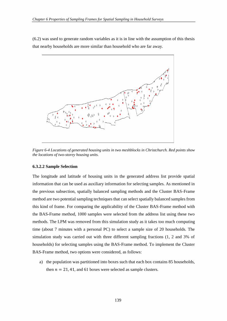
Chapter 6 Properties of Sampling Frames for Spatial Sampling in Household Surveys
139
(6.2) was used to generate random variables as it is in line with the assumption of this thesis
that nearby households are more similar than household who are far away.
Figure 6-4 Locations of generated housing units in two meshblocks in Christchurch. Red points show
the locations of two-storey housing units.
6.3.2.2 Sample Selection
The longitude and latitude of housing units in the generated address list provide spatial
information that can be used as auxiliary information for selecting samples. As mentioned in
the previous subsection, spatially balanced sampling methods and the Cluster BAS-Frame
method are two potential sampling techniques that can select spatially balanced samples from
this kind of frame. For comparing the applicability of the Cluster BAS-Frame method with
the BAS-Frame method, 1000 samples were selected from the address list using these two
methods. The LPM was removed from this simulation study as it takes too much computing
time (about 7 minutes with a personal PC) to select a sample size of 20 households. The
simulation study was carried out with three different sampling fractions (1, 2 and 3% of
households) for selecting samples using the BAS-Frame method. To implement the Cluster
BAS-Frame method, two options were considered, as follows:
a) the population was partitioned into boxes such that each box contains 85 households,
then 𝑛 = 21, 41, and 61 boxes were selected as sample clusters.
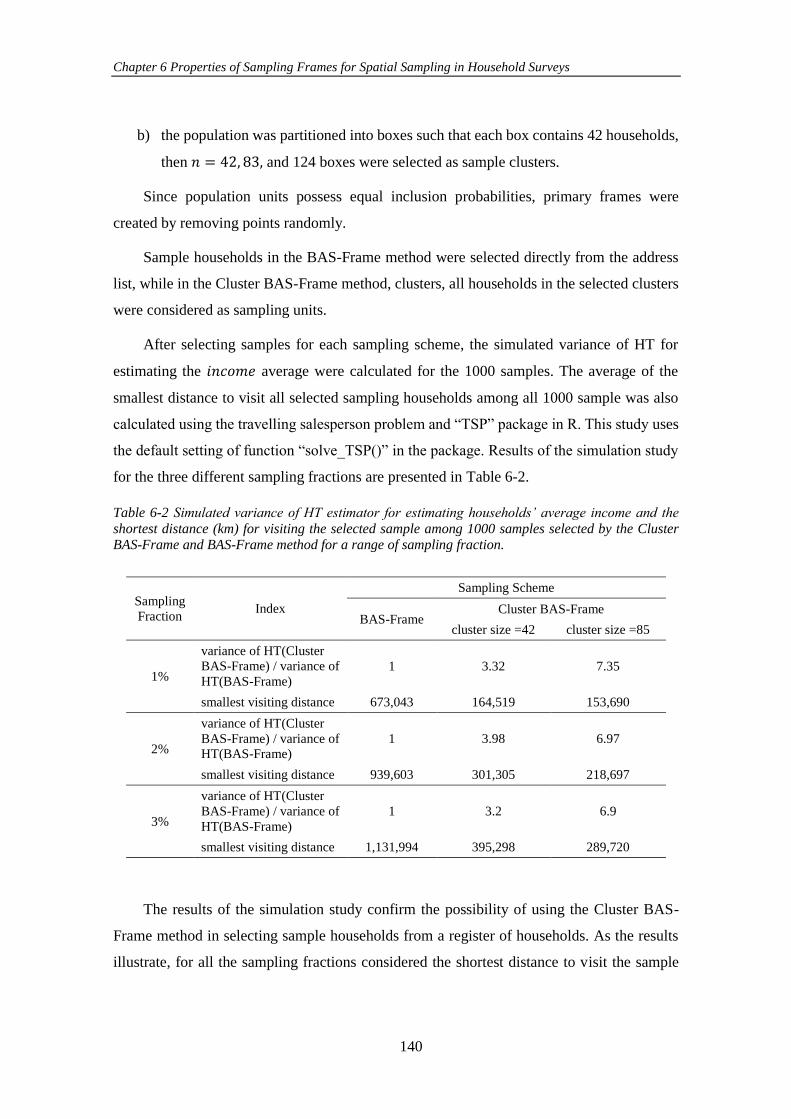
Chapter 6 Properties of Sampling Frames for Spatial Sampling in Household Surveys
140
b) the population was partitioned into boxes such that each box contains 42 households,
then 𝑛 = 42, 83, and 124 boxes were selected as sample clusters.
Since population units possess equal inclusion probabilities, primary frames were
created by removing points randomly.
Sample households in the BAS-Frame method were selected directly from the address
list, while in the Cluster BAS-Frame method, clusters, all households in the selected clusters
were considered as sampling units.
After selecting samples for each sampling scheme, the simulated variance of HT for
estimating the 𝑖𝑛𝑐𝑜𝑚𝑒 average were calculated for the 1000 samples. The average of the
smallest distance to visit all selected sampling households among all 1000 sample was also
calculated using the travelling salesperson problem and “TSP” package in R. This study uses
the default setting of function “solve_TSP()” in the package. Results of the simulation study
for the three different sampling fractions are presented in Table 6-2.
Table 6-2 Simulated variance of HT estimator for estimating households’ average income and the
shortest distance (km) for visiting the selected sample among 1000 samples selected by the Cluster BAS-Frame and BAS-Frame method for a range of sampling fraction.
Sampling
Fraction Index
Sampling Scheme
BAS-Frame Cluster BAS-Frame
cluster size =42 cluster size =85
1%
variance of HT(Cluster
BAS-Frame) / variance of
HT(BAS-Frame)
1 3.32 7.35
smallest visiting distance 673,043 164,519 153,690
2%
variance of HT(Cluster
BAS-Frame) / variance of
HT(BAS-Frame)
1 3.98 6.97
smallest visiting distance 939,603 301,305 218,697
3%
variance of HT(Cluster
BAS-Frame) / variance of
HT(BAS-Frame)
1 3.2 6.9
smallest visiting distance 1,131,994 395,298 289,720
The results of the simulation study confirm the possibility of using the Cluster BAS-
Frame method in selecting sample households from a register of households. As the results
illustrate, for all the sampling fractions considered the shortest distance to visit the sample
Chapter 6 Properties of Sampling Frames for Spatial Sampling in Household Surveys
141
households is significantly higher in the BAS-Frame method compared with the Cluster BAS-
Frame method. This is because Cluster BAS-Frame selects a group of households that are
located geographically near to each other. Table 6-2 shows that in a fixed sample size, by
increasing the size of clusters, the shortest distance to visit all the sample households is
decreased. The smallest visiting distances achieved confirm that using the Cluster BAS-
Frame method can decrease the sampling cost.
Cluster BAS-Frame selects spatially balanced clusters; however, it may not be
considered a spatially balanced sampling method in terms of selecting ultimate sampling
units. Comparing the simulated variance of HT among the two sampling methods evaluated
shows that the BAS-Frame technique provides more precise estimates than the Cluster BAS-
Frame method.
According to the results achieved, employing the Cluster BAS-Frame is recommended
in situations when the available sampling frame is a list of households in the population and
there is an interest to decrease the sample costs in an in-person survey.
6.4 Application of Spatially Balanced Sampling Methods in Household
Surveys in Non-ideal Situations
Up to this section, spatially balanced sampling methods were employed for selecting samples
in ideal situations where either an area or list frame of the sampling units is available (i.e.,
selecting a sample of Christchurch meshblocks from a list including the geographical
coordinates of the centre of Christchurch meshblocks). However, sometimes surveys need to
be conducted in non-ideal conditions. Conducting a survey immediately after a disaster (e.g.,
an earthquake) or drawing a sample from war areas that have not had a census for a decade
are two examples of non-ideal conditions. These situations are called non-ideal conditions as
there is no reliable sampling frame for the population units and consequently the usual
sampling methods, such as cluster or stratified sampling, might not be used as well as they
could be, for gathering information.
Fortunately, recent advances in GIS and spatial tools have been shown to be helpful
when conducting sampling surveys in non-ideal situations. For instance, Elangovan et al.
(2016) used GIS/GPS-based grid-sampling method to study tuberculosis in Thiruneermalai,
India. They overlaid a 30 × 30 metre small grid on the area of the population under study and
selected 300 grid cells, using a simple random sampling method, as the sampling units. In
Chapter 6 Properties of Sampling Frames for Spatial Sampling in Household Surveys
142
another study, on the migrants in Beijing, Landry and Shen (2005) designed a spatial
sampling method to overcome the lack of complete coverage in traditional samples, in which
the selections had been based on household lists. They firstly created a spatial grid of Beijing
and then selected some cells randomly as sampling units. They demonstrated that their
method reduced the coverage bias compared with traditional methods.
Most recently Thomson et al. (2017) have provided an R package to select samples from
gridded population data. In their study, they used gridded population data as an alternative
sample frame where census data was outdated or unreliable. The Gridded Population of the
World (GPWv4), the Global Rural-Urban Mapping Project (GRUMP), LAndScan (LandScan
Data Availability, 2017), WordPop (Stevens, F. et al., 2015), and Demobase (Azar et al.,
2013) are examples of gridded populations that are available to freely download. Using the
gridded population data, Galway et al. (2012) also designed a two-stage cluster sampling to
study mortality in Iraq.
Kolbe et al. (2010) conducted a spatial sampling design to provide a rapid assessment of
the population of the metropolitan area of Port-au-Prince soon after the earthquake of January
2010. They provided the geographic boundaries of the area at the first step and then selected
a sample of GPS coordinates randomly within the metropolitan area. Other studies that have
used spatial techniques to overcome the lack of sampling frames in households surveys can
be found in Kondo et al. (2014), Haenssgen (2015), Siri et al. (2008), Shannon et al. (2012),
Varona and Tabernilla (2013), Singh and Clark (2012).
6.4.1 Selecting a Spatially Balanced Sample From a Map Using the BAS Method
As discussed earlier, geographical information about the population under study is typically
the only information that can be provided in a sampling frame in a non-ideal situation. In
most situations, this frame is a map containing the geographic boundaries of different areas
of the population. In this study, this kind of frame is called a map frame and might be provided
using GIS technology. Figure 6-5 is an example of a map frame from a small part of
Christchurch city.
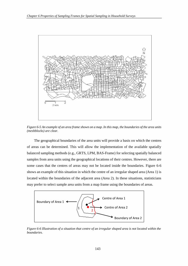
Chapter 6 Properties of Sampling Frames for Spatial Sampling in Household Surveys
143
Figure 6-5 An example of an area frame shown on a map. In this map, the boundaries of the area units
(meshblocks) are clear.
The geographical boundaries of the area units will provide a basis on which the centres
of areas can be determined. This will allow the implementation of the available spatially
balanced sampling methods (e.g., GRTS, LPM, BAS-Frame) for selecting spatially balanced
samples from area units using the geographical locations of their centres. However, there are
some cases that the centres of areas may not be located inside the boundaries. Figure 6-6
shows an example of this situation in which the centre of an irregular shaped area (Area 1) is
located within the boundaries of the adjacent area (Area 2). In these situations, statisticians
may prefer to select sample area units from a map frame using the boundaries of areas.
Figure 6-6 Illustration of a situation that centre of an irregular shaped area is not located within the
boundaries.
Centre of Area 1Boundary of Area 1
12
Centre of Area 2
Boundary of Area 2
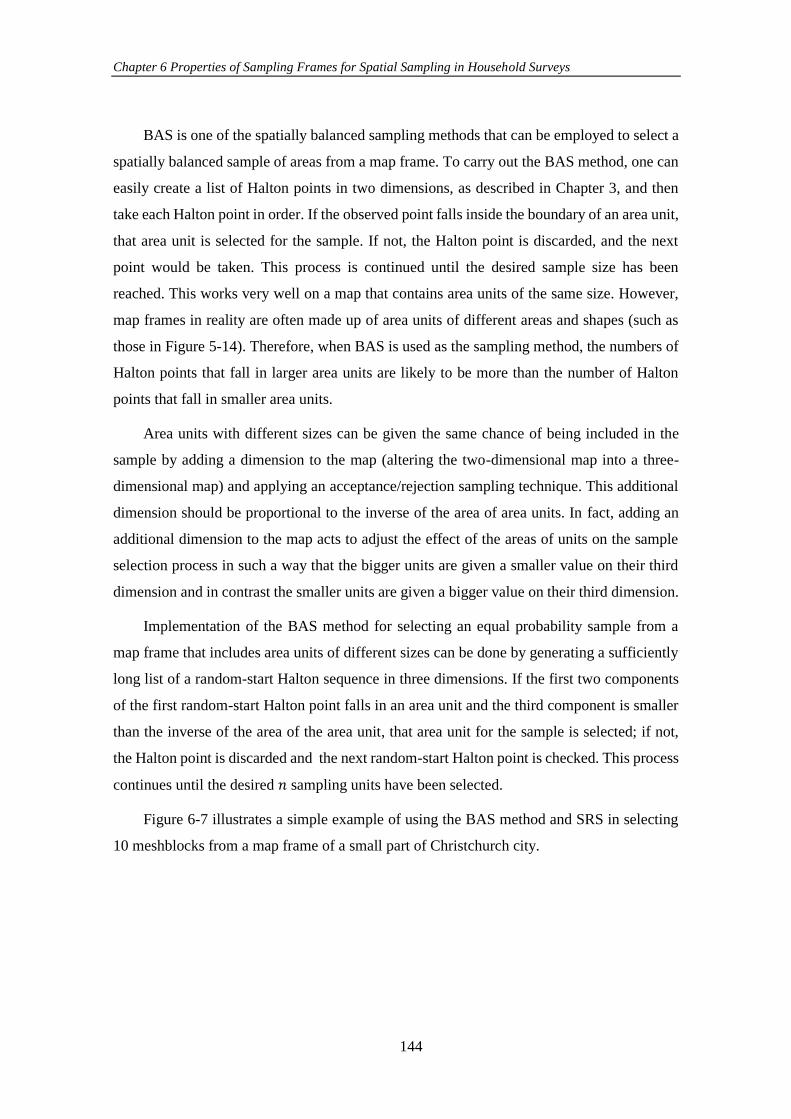
Chapter 6 Properties of Sampling Frames for Spatial Sampling in Household Surveys
144
BAS is one of the spatially balanced sampling methods that can be employed to select a
spatially balanced sample of areas from a map frame. To carry out the BAS method, one can
easily create a list of Halton points in two dimensions, as described in Chapter 3, and then
take each Halton point in order. If the observed point falls inside the boundary of an area unit,
that area unit is selected for the sample. If not, the Halton point is discarded, and the next
point would be taken. This process is continued until the desired sample size has been
reached. This works very well on a map that contains area units of the same size. However,
map frames in reality are often made up of area units of different areas and shapes (such as
those in Figure 5-14). Therefore, when BAS is used as the sampling method, the numbers of
Halton points that fall in larger area units are likely to be more than the number of Halton
points that fall in smaller area units.
Area units with different sizes can be given the same chance of being included in the
sample by adding a dimension to the map (altering the two-dimensional map into a three-
dimensional map) and applying an acceptance/rejection sampling technique. This additional
dimension should be proportional to the inverse of the area of area units. In fact, adding an
additional dimension to the map acts to adjust the effect of the areas of units on the sample
selection process in such a way that the bigger units are given a smaller value on their third
dimension and in contrast the smaller units are given a bigger value on their third dimension.
Implementation of the BAS method for selecting an equal probability sample from a
map frame that includes area units of different sizes can be done by generating a sufficiently
long list of a random-start Halton sequence in three dimensions. If the first two components
of the first random-start Halton point falls in an area unit and the third component is smaller
than the inverse of the area of the area unit, that area unit for the sample is selected; if not,
the Halton point is discarded and the next random-start Halton point is checked. This process
continues until the desired 𝑛 sampling units have been selected.
Figure 6-7 illustrates a simple example of using the BAS method and SRS in selecting
10 meshblocks from a map frame of a small part of Christchurch city.
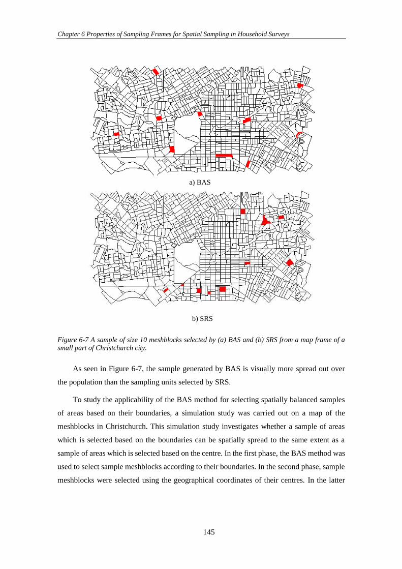
Chapter 6 Properties of Sampling Frames for Spatial Sampling in Household Surveys
145
Figure 6-7 A sample of size 10 meshblocks selected by (a) BAS and (b) SRS from a map frame of a small part of Christchurch city.
As seen in Figure 6-7, the sample generated by BAS is visually more spread out over
the population than the sampling units selected by SRS.
To study the applicability of the BAS method for selecting spatially balanced samples
of areas based on their boundaries, a simulation study was carried out on a map of the
meshblocks in Christchurch. This simulation study investigates whether a sample of areas
which is selected based on the boundaries can be spatially spread to the same extent as a
sample of areas which is selected based on the centre. In the first phase, the BAS method was
used to select sample meshblocks according to their boundaries. In the second phase, sample
meshblocks were selected using the geographical coordinates of their centres. In the latter
a) BAS
b) SRS
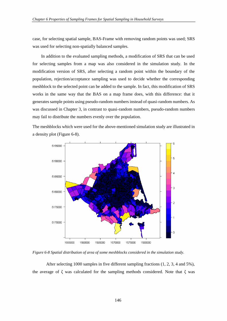
Chapter 6 Properties of Sampling Frames for Spatial Sampling in Household Surveys
146
case, for selecting spatial sample, BAS-Frame with removing random points was used; SRS
was used for selecting non-spatially balanced samples.
In addition to the evaluated sampling methods, a modification of SRS that can be used
for selecting samples from a map was also considered in the simulation study. In the
modification version of SRS, after selecting a random point within the boundary of the
population, rejection/acceptance sampling was used to decide whether the corresponding
meshblock to the selected point can be added to the sample. In fact, this modification of SRS
works in the same way that the BAS on a map frame does, with this difference: that it
generates sample points using pseudo-random numbers instead of quasi-random numbers. As
was discussed in Chapter 3, in contrast to quasi-random numbers, pseudo-random numbers
may fail to distribute the numbers evenly over the population.
The meshblocks which were used for the above-mentioned simulation study are illustrated in
a density plot (Figure 6-8).
Figure 6-8 Spatial distribution of area of some meshblocks considered in the simulation study.
After selecting 1000 samples in five different sampling fractions (1, 2, 3, 4 and 5%),
the average of ζ was calculated for the sampling methods considered. Note that ζ was
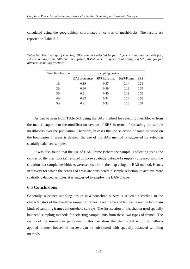
Chapter 6 Properties of Sampling Frames for Spatial Sampling in Household Surveys
147
calculated using the geographical coordinates of centres of meshblocks. The results are
reported in Table 6-3.
Table 6-3 The average of 𝜁 among 1000 samples selected by four different sampling methods (i.e.,
BAS on a map frame, SRS on a map frame, BAS-Frame using centre of areas, and SRS) and for five
different sampling fractions.
Sampling fraction Sampling design
BAS from map SRS from map BAS-Frame SRS
1% 0.19 0.37 0.14 0.38
2% 0.20 0.39 0.12 0.37
3% 0.21 0.40 0.12 0.39
4% 0.22 0.34 0.14 0.33
5% 0.21 0.33 0.13 0.37
As can be seen from Table 6-3, using the BAS method for selecting meshblocks from
the map is superior to the modification version of SRS in terms of spreading the sample
meshblocks over the population. Therefore, in cases that the selection of samples based on
the boundaries of areas is desired, the use of the BAS method is suggested for selecting
spatially balanced samples.
It was also found that the use of BAS-Frame (where the sample is selecting using the
centres of the meshblocks) resulted in more spatially balanced samples compared with the
situation that sample meshblocks were selected from the map using the BAS method. Hence,
in surveys for which the centres of areas are considered in sample selection, to achieve more
spatially balanced samples, it is suggested to employ the BAS-Frame.
6.5 Conclusions
Generally, a proper sampling design in a household survey is selected according to the
characteristics of the available sampling frames. Area frame and list frame are the two main
kinds of sampling frames in household surveys. The first section of this chapter used spatially
balanced sampling methods for selecting sample units from these two types of frames. The
results of the simulations performed in this part show that the current sampling methods
applied in most household surveys can be substituted with spatially balanced sampling
methods.
Chapter 6 Properties of Sampling Frames for Spatial Sampling in Household Surveys
148
After introducing the new sampling frames, which are mostly used in developed
countries, the application of spatially balanced sampling methods for selecting samples from
these kinds of frames was investigated in the second section. Although employing spatially
balanced sampling methods in the presence of the new format of sampling frames can provide
more precise estimates, it may cause a high sampling cost. This drawback was addressed by
modifying the BAS-Frame method. This modified version, the Cluster BAS-Frame method,
decreases the survey cost by selecting units near to each other. It follows the same rationale
as the BAS-method for putting the population units into clusters of more than one unit. It then
uses the BAS method for selecting a spatial sample cluster as sampling units at the first stage
of a multi-stage sampling process. The simulation study in this part showed that the shortest
distance to visit all the selected sampling units can be halved when the samples were selected
by the Cluster BAS-Frame method instead of the BAS-Frame method.
The application of spatially balanced sampling methods in a non-ideal situation where
there exists no ordinary sampling frame was explained in the third section. After providing a
map of the population of interest and defining the geographical centre of areas, the available
spatially balanced sampling methods can be applied to select sample units. However, there
are cases where statisticians prefer to select sample areas based on their geographical
boundaries. Among the spatially balanced sampling methods, BAS can be used for selecting
a sample directly from a map of area units that are defined only by their boundaries. This can
be done by introducing an extra dimension relevant to the inverse of the area of each unit and
then implementing an acceptance/rejection technique. A simulation study was conducted to
compare the efficiency of the BAS method with the BAS-Frame method and a modified
version of SRS in terms of selecting spatially balanced sample areas from a map. The results
illustrated that the BAS method could generally select more spatially balanced samples
compared to the modified version of SRS. In addition, it was found that the implementation
of the BAS-Frame method on the basis of the centres of the areas provided more spatially
balanced samples compared with the situation where sample areas were selected from the
map using the BAS method.
6.6 References
Azar, D., Engstrom, R., Graesser, J., & Comenetz, J. (2013). Generation of fine-scale population
layers using multi-resolution satellite imagery and geospatial data. Remote Sensing of
Environment, 130, 219-232.
Chapter 6 Properties of Sampling Frames for Spatial Sampling in Household Surveys
149
Bycroft, C. (2011). Future New Zealand censuses: Implications of changing census frequency or
adopting other models: Wellington: Statistics New Zealand ISBN.
Centers for Disease Control. (2010). Global Adult Tobacco Survey Collaborative Group. Global
Adult Tobacco Survey (GATS): Core Questionnaire with Optional Questions, Version
2.0. Atlanta, GA.–2010.–56 р.
Cooper, S. L. (1964). Random sampling by telephone: an improved method. Journal of Marketing
Research, 45-48.
Darkwah, K. A., Nortey, E. N., & Lotsi, A. (2016). Estimation of the Gini coefficient for the
lognormal distribution of income using the Lorenz curve. SpringerPlus, 5(1), 1196.
Elangovan, A., Elavarsu, G., Ezhil, R., Prabu, R., & Yuvaraj, J. (2016). Geospatial Techniques in
Health Survey to Overcome the Lack of Sampling Frame. International Journal of
Advanced Remote Sensing and GIS, pp. 1908-1914.
Galway, L. P., Bell, N., Al Shatari, S. A., Hagopian, A., Burnham, G., Flaxman, A., Weiss, W.
M., Rajaratnam, J., & Takaro, T. K. (2012). A two-stage cluster sampling method using
gridded population data, a GIS, and Google Earth TM imagery in a population-based
mortality survey in Iraq. International journal of health geographics, 11(1), 12.
GPWv4. Gridded Population of the World v4. Center for International Earth Science Information
Network, Columbia University, New York. 2016. . Retrieved from
https://sedac.ciesin.columbia.edu/data/collection/gpw-v4/sets/browse
GRUMP. Gridded Rural Urban Mapping Project v1. Center for International Earth Science
Information Network, Columbia University, New York. 2006. . Retrieved from
http://sedac.ciesin.columbia.edu/data/set/grump-v1-population-count/data-download
Haenssgen, M. J. (2015). Satellite-aided survey sampling and implementation in low-and middle-
income contexts: a low-cost/low-tech alternative. Emerging themes in epidemiology,
12(1), 20.
Hajek, J., & Dupac, V. (1981). Sampling from a finite population (Vol. 37). New York: M.
Dekker.
Holzer, C., Spitznagel, E., Jordan, K., Timbers, D., Kessler, L., & Anthony, J. (1985). Sampling
the household population. Epidemiologic field methods in psychiatry: The NIMH
Epidemiologic Catchment Area program, 285-308.
ICF, I. (2012). Demographic and Health Survey sampling and household listing manual. In: ICF
International Maryland, USA.
Kolbe, A. R., Hutson, R. A., Shannon, H., Trzcinski, E., Miles, B., Levitz, N., Puccio, M., James,
L., Noel, J. R., & Muggah, R. (2010). Mortality, crime and access to basic needs before
and after the Haiti earthquake: a random survey of Port-au-Prince households. Medicine,
conflict and survival, 26(4), 281-297.
Kondo, M. C., Bream, K. D., Barg, F. K., & Branas, C. C. (2014). A random spatial sampling
method in a rural developing nation. BMC public health, 14(1), 338.
Landry, P. F., & Shen, M. (2005). Reaching migrants in survey research: the use of the global
positioning system to reduce coverage bias in China. Political Analysis, 13(1), 1-22.
LandScan Data Availability. Oak Ridge National Laboratories, Oak Ridge, Tennessee. . (2017).
Retrieved from http://www.ornl.gov/sci/landscan/landscan_data_avail.shtml
Chapter 6 Properties of Sampling Frames for Spatial Sampling in Household Surveys
150
Link, M. W., Battaglia, M. P., Frankel, M. R., Osborn, L., & Mokdad, A. H. (2008). A comparison
of address-based sampling (ABS) versus random-digit dialing (RDD) for general
population surveys. Public Opinion Quarterly, 72(1), 6-27.
Poulain, M., Herm, A., & Depledge, R. (2013). Central population registers as a source of
demographic statistics in Europe. Population, 68(2), 183-212.
R Core Team. (2017). R: A language and environment for statistical computing. R Foundation
for Statistical Computing, Vienna, Austria. URL https://www. R-project. org.
Robertson, B., Brown, J., McDonald, T., & Jaksons, P. (2013). BAS: balanced acceptance
sampling of natural resources. Biometrics, 69(3), 776-784.
Särndal, C.-E., Swensson, B., & Wretman, J. (2003). Model assisted survey sampling: Springer
Science & Business Media.
Scherpenzeel, A., Maineri, A., Bristle, J., Pflüger, S.-M., Mindarova, I., Butt, S., Zins, S., Emery,
T., & Luijkx, R. (2017). Report on the use of sampling frames in European studies.
Retrieved from Deliverable 2.1 of the SERISS project funded under the European
Union’s Horizon 2020 research and innovation programme GA No: 654221. Available
at: www.seriss.eu/resources/deliverables.
Shannon, H. S., Hutson, R., Kolbe, A., Stringer, B., & Haines, T. (2012). Choosing a survey
sample when data on the population are limited: a method using Global Positioning
Systems and aerial and satellite photographs. Emerging themes in epidemiology, 9(1), 5.
Singh, G., & Clark, B. D. (2012). Creating a frame: A spatial approach to random sampling of
immigrant households in inner city Johannesburg. Journal of Refugee Studies, 26(1), 126-
144.
Siri, J. G., Lindblade, K. A., Rosen, D. H., Onyango, B., Vulule, J. M., Slutsker, L., & Wilson,
M. L. (2008). A census-weighted, spatially-stratified household sampling strategy for
urban malaria epidemiology. Malaria journal, 7(1), 39.
Stevens, D., & Olsen, A. (2004). Spatially balanced sampling of natural resources. Journal of the
American Statistical Association, 99(465), 262-278.
Stevens, F., Gaughan, A. E., Linard, C., & Tatem, A. J. (2015). Disaggregating census data for
population mapping using random forests with remotely-sensed and ancillary data. PLoS
ONE, 10(2), e0107042.
Thomson, D. R., Stevens, F. R., Ruktanonchai, N. W., Tatem, A. J., & Castro, M. C. (2017).
GridSample: an R package to generate household survey primary sampling units (PSUs)
from gridded population data. International journal of health geographics, 16(1), 25.
Turner, A. G. (2003). Sampling strategies. Handbook on designing of household sample surveys.
Geneva: United Nations Statistics Division.
United Nations-Statistical Division. (2008). Designing household survey samples: practical
guidelines (Vol. 98): United Nations Publications.
United States Postal Service. Retrieved from https://www.usps.com/
Varona, F. C., & Tabernilla, J. O. (2013). Improving the sampling srame for household-based
surveys using digitized satellite maps. Paper presented at the 12th National Convention
on Statistics (NCS), EDSA Shangri-La Hotel, Mandaluyong City.
151
Spatially Balanced Sampling Methods and
Some Features of Household Surveys
7.1 Introduction
In the previous chapter, the application of spatially balanced sampling methods for selecting
samples from different types of sampling frames in household surveys was investigated. In
practice, household surveys often have specific requirements, for instance, the need to
monitor an estimate of a parameter of interest over time, with demands for a particular survey
design. This chapter describes how spatially balanced sampling methods can be used in these
situations.
Constructing primary sampling units (PSUs) that are of pre-specified size and contain
neighbouring units is one of these situations that will be discussed in the first section. The
second section explains how spatially balanced sampling methods can be used in a
longitudinal survey. Avoiding selection of the same units with multiple surveys is one
challenge in household surveys that will be discussed in this section. Finally, the third section
investigates how auxiliary variables can be used in designing a spatially balanced sampling
method. A simulation study, based on real data, is used to investigate the efficiency of
spatially balanced sampling with auxiliary variables.
7.2 Constructing PSUs in Household Surveys
Defining PSUs is one of the most important, and sometimes grueling processes, in designing
a household sampling survey. Although natural geographical areas (such as meshblocks or
counties) are considered to be practically the best candidates in terms of allocation of
interviewers to areas and controlling the survey cost for PSUs in most household surveys,
they often need to be modified or adjusted before being used as PSUs (Yansaneh, 2005). This
modification is done to ensure that the selected PSUs include enough sampling units
(Yansaneh, 2005). In fact, there is usually a requirement of having a pre-specified minimum
number of secondary sampling units per PSUs.
Chapter 7 Spatially Balanced Sampling Methods and Some Features of Household Surveys
152
Extremely large geographical units can usually be split into a number of smaller
subunits, with one randomly selected as the PSU. This is called “segmentation“. Another way
to deal with extremely large geographical units that must be represented in the survey is to
treat them as separate strata. In this situation, each large PSU is located in a separate stratum
which is called a “certainty” or “self-representing” PSU (Kalton & Anderson, 1986). A self-
representing PSU is in fact a stratum with only one member that is selected in the first stage
of the sample selection process.
Undersized geographical units have sizes (e.g., number of their households) that are
smaller than a pre-specified size and are usually combined with bigger ones to create PSUs
which satisfy a pre-specified size. In the process of defining PSUs, dealing with undersized
PSUs is generally more challenging than dealing with oversized PSUs. That is because
combining undersized PSUs needs to be done prior to the selection of PSU. Whereas, the
partitioning required for the oversized PSUs is done only when an oversized PSU has been
selected. This section focuses on providing a simple method for combining adjacent
undersized PSUs.
A procedure for combining PSUs during or after sample selection was first introduced
by Kish (1965). After preparing a list of population units along with their size, the Kish
method searches for the units which are either below the pre-specified size or immediately
follow a unit below the pre-specified size. It then combines such units together. The list of
population units can, for instance, be provided by ordering population units with respect to
their longitude. Units with the same longitude are then ordered by their latitude. Given that
units which are located geographically close to each other are listed near to each other on the
list (e.g., when the serpentine ordering (Williams & Chromy, 1980) is used to sort units in a
frame), this method tries to combine undersized nearby units with each other. The following
example illustrates the procedure.
Example 7.1
Consider a population of 16 geographical units, labelled A, B, …, P. Let the size of each
unit be defined by the number of households it contains. Here, the units are ordered firstly by
their longitude and then by their latitude. Geographical units along with their sizes are shown
in Table 7-1.
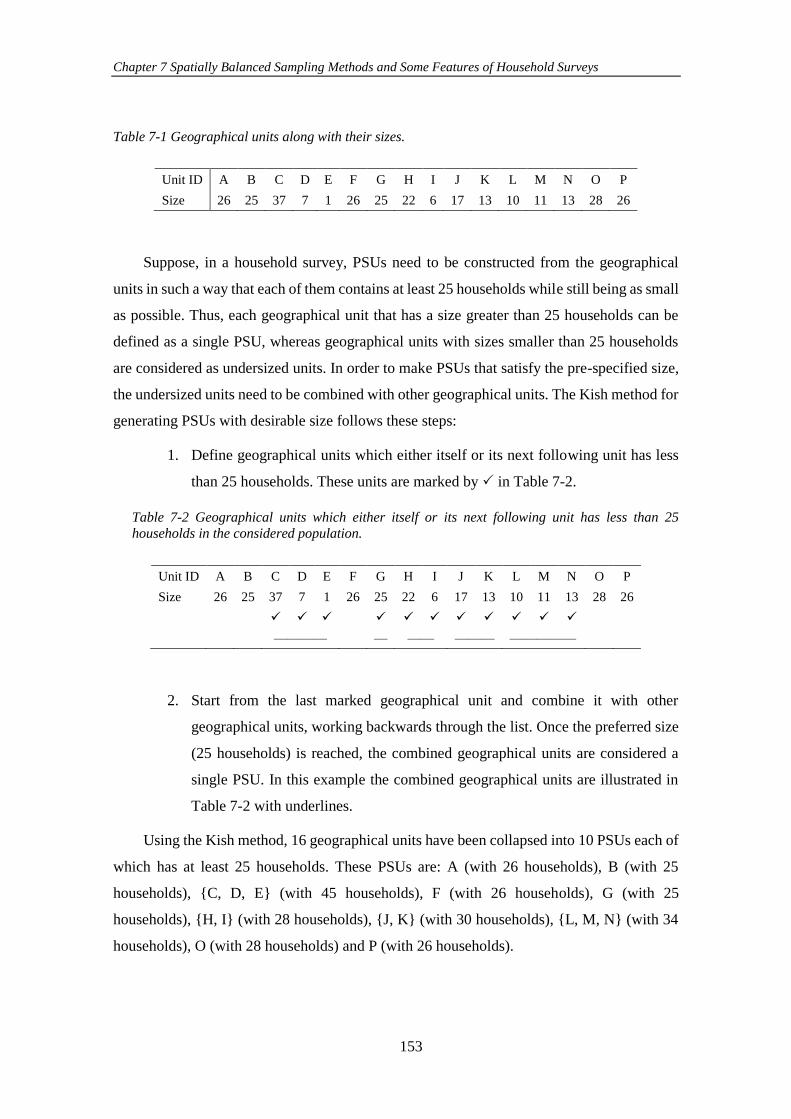
Chapter 7 Spatially Balanced Sampling Methods and Some Features of Household Surveys
153
Table 7-1 Geographical units along with their sizes.
Unit ID A B C D E F G H I J K L M N O P
Size 26 25 37 7 1 26 25 22 6 17 13 10 11 13 28 26
Suppose, in a household survey, PSUs need to be constructed from the geographical
units in such a way that each of them contains at least 25 households while still being as small
as possible. Thus, each geographical unit that has a size greater than 25 households can be
defined as a single PSU, whereas geographical units with sizes smaller than 25 households
are considered as undersized units. In order to make PSUs that satisfy the pre-specified size,
the undersized units need to be combined with other geographical units. The Kish method for
generating PSUs with desirable size follows these steps:
1. Define geographical units which either itself or its next following unit has less
than 25 households. These units are marked by in Table 7-2.
Table 7-2 Geographical units which either itself or its next following unit has less than 25
households in the considered population.
Unit ID A B C D E F G H I J K L M N O P
Size 26 25 37 7 1 26 25 22 6 17 13 10 11 13 28 26
———— — —— ——— —————
2. Start from the last marked geographical unit and combine it with other
geographical units, working backwards through the list. Once the preferred size
(25 households) is reached, the combined geographical units are considered a
single PSU. In this example the combined geographical units are illustrated in
Table 7-2 with underlines.
Using the Kish method, 16 geographical units have been collapsed into 10 PSUs each of
which has at least 25 households. These PSUs are: A (with 26 households), B (with 25
households), {C, D, E} (with 45 households), F (with 26 households), G (with 25
households), {H, I} (with 28 households), {J, K} (with 30 households), {L, M, N} (with 34
households), O (with 28 households) and P (with 26 households).
Chapter 7 Spatially Balanced Sampling Methods and Some Features of Household Surveys
154
7.2.1 Using the BAS-Frame Technique for Combining Undersized Neighbouring
Units
The Kish method combines PSUs according to their order in a list and there is no guarantee
that the created PSUs would be constructed of nearby geographical units. Hence, the Kish
method is not recommended for cases where there are a large number of undersized PSUs
(Yansaneh, 2005) and PSUs need to contain nearby units.
Thomson et al. (2017) introduced a method for constructing PSUs when gridded
population data are used as the sampling frame rather than census data. In their method, some
cells (based on the sample size) are selected randomly from the gridded dataset in the first
step as “PSU seed cells”, and then the selected PSU seed cells will grow by adding
neighboring cells one cell a time until a minimum PSU size is achieved. Each PSU seed cell
will be expanded by randomly adding one of the nearest north, east, south, or west cells to
the PSU. In this method, after selecting PSU seed cells, Voronoi polygons around each PSU
seed cell are drawn, and the PSU growth is restricted inside the Voronoi polygons around
each selected PSU seed cell. This ensures that the created PSUs do not overlap.
In this subsection a technique for combining undersized units in two-dimensional
populations – defined by their geographical coordinates (latitude and longitude) – will be
introduced. The method introduced by Thomson et al. (2017) only works on gridded
population data, whereas the proposed method can work on all kind of datasets that contain
geographical coordinates of units (i.e., census data and gridded population data). Another
advantage of this method is that it provides a list of desirable sized PSUs that can be used as
a sampling frame for a number of household surveys, not only a specific survey. Another
difference between the proposed method and the Thomson et al. (2017) method is that there
is no need to select PSUs seed cells or define Voronoi polygons.
The proposed technique is based on the rationale of the BAS-Frame method and should
be implemented before employing the sample selection process. Similar to the BAS-Frame
method, this technique provides a frame by partitioning the primary units (e.g., meshblocks)
sequentially along their latitude and longitude. However, in this technique, the partitioning
process is undertaken irrespective of the size of the primary units (e.g., number of households
in each meshblock). In fact, the population is partitioned such that the creation of boxes
smaller than a pre-specified size would be prevented. For this, the partition proposed in each
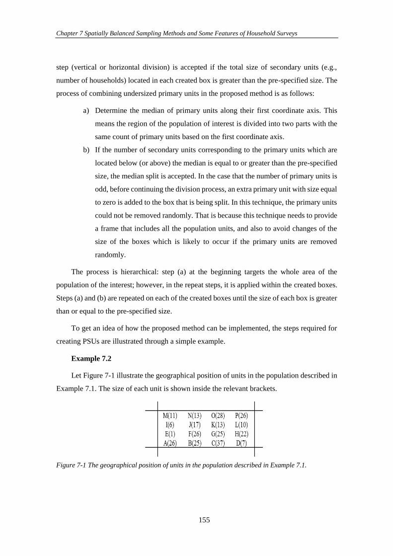
Chapter 7 Spatially Balanced Sampling Methods and Some Features of Household Surveys
155
step (vertical or horizontal division) is accepted if the total size of secondary units (e.g.,
number of households) located in each created box is greater than the pre-specified size. The
process of combining undersized primary units in the proposed method is as follows:
a) Determine the median of primary units along their first coordinate axis. This
means the region of the population of interest is divided into two parts with the
same count of primary units based on the first coordinate axis.
b) If the number of secondary units corresponding to the primary units which are
located below (or above) the median is equal to or greater than the pre-specified
size, the median split is accepted. In the case that the number of primary units is
odd, before continuing the division process, an extra primary unit with size equal
to zero is added to the box that is being split. In this technique, the primary units
could not be removed randomly. That is because this technique needs to provide
a frame that includes all the population units, and also to avoid changes of the
size of the boxes which is likely to occur if the primary units are removed
randomly.
The process is hierarchical: step (a) at the beginning targets the whole area of the
population of the interest; however, in the repeat steps, it is applied within the created boxes.
Steps (a) and (b) are repeated on each of the created boxes until the size of each box is greater
than or equal to the pre-specified size.
To get an idea of how the proposed method can be implemented, the steps required for
creating PSUs are illustrated through a simple example.
Example 7.2
Let Figure 7-1 illustrate the geographical position of units in the population described in
Example 7.1. The size of each unit is shown inside the relevant brackets.
Figure 7-1 The geographical position of units in the population described in Example 7.1.
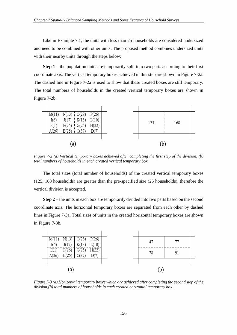
Chapter 7 Spatially Balanced Sampling Methods and Some Features of Household Surveys
156
Like in Example 7.1, the units with less than 25 households are considered undersized
and need to be combined with other units. The proposed method combines undersized units
with their nearby units through the steps below:
Step 1 – the population units are temporarily split into two parts according to their first
coordinate axis. The vertical temporary boxes achieved in this step are shown in Figure 7-2a.
The dashed line in Figure 7-2a is used to show that these created boxes are still temporary.
The total numbers of households in the created vertical temporary boxes are shown in
Figure 7-2b.
Figure 7-2 (a) Vertical temporary boxes achieved after completing the first step of the division, (b)
total numbers of households in each created vertical temporary box.
The total sizes (total number of households) of the created vertical temporary boxes
(125, 168 households) are greater than the pre-specified size (25 households), therefore the
vertical division is accepted.
Step 2 – the units in each box are temporarily divided into two parts based on the second
coordinate axis. The horizontal temporary boxes are separated from each other by dashed
lines in Figure 7-3a. Total sizes of units in the created horizontal temporary boxes are shown
in Figure 7-3b.
Figure 7-3 (a) Horizontal temporary boxes which are achieved after completing the second step of the
division,(b) total numbers of households in each created horizontal temporary box.
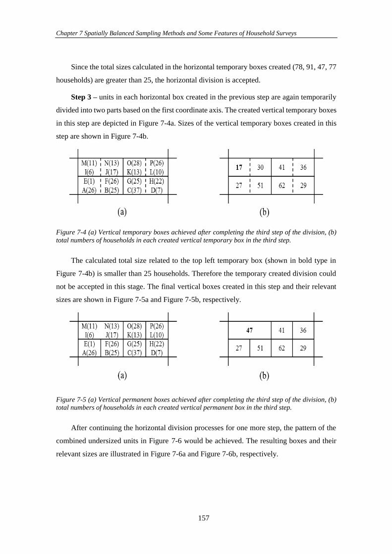
Chapter 7 Spatially Balanced Sampling Methods and Some Features of Household Surveys
157
Since the total sizes calculated in the horizontal temporary boxes created (78, 91, 47, 77
households) are greater than 25, the horizontal division is accepted.
Step 3 – units in each horizontal box created in the previous step are again temporarily
divided into two parts based on the first coordinate axis. The created vertical temporary boxes
in this step are depicted in Figure 7-4a. Sizes of the vertical temporary boxes created in this
step are shown in Figure 7-4b.
Figure 7-4 (a) Vertical temporary boxes achieved after completing the third step of the division, (b)
total numbers of households in each created vertical temporary box in the third step.
The calculated total size related to the top left temporary box (shown in bold type in
Figure 7-4b) is smaller than 25 households. Therefore the temporary created division could
not be accepted in this stage. The final vertical boxes created in this step and their relevant
sizes are shown in Figure 7-5a and Figure 7-5b, respectively.
Figure 7-5 (a) Vertical permanent boxes achieved after completing the third step of the division, (b) total numbers of households in each created vertical permanent box in the third step.
After continuing the horizontal division processes for one more step, the pattern of the
combined undersized units in Figure 7-6 would be achieved. The resulting boxes and their
relevant sizes are illustrated in Figure 7-6a and Figure 7-6b, respectively.
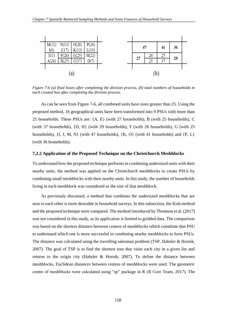
Chapter 7 Spatially Balanced Sampling Methods and Some Features of Household Surveys
158
Figure 7-6 (a) final boxes after completing the division process, (b) total numbers of households in
each created box after completing the division process.
As can be seen from Figure 7-6, all combined units have sizes greater than 25. Using the
proposed method, 16 geographical units have been transformed into 9 PSUs with more than
25 households. These PSUs are: {A, E} (with 27 households), B (with 25 households), C
(with 37 households), {D, H} (with 29 households), F (with 26 households), G (with 25
households), {I, J, M, N} (with 47 households), {K, O} (with 41 households) and {P, L}
(with 36 households).
7.2.2 Application of the Proposed Technique on the Christchurch Meshblocks
To understand how the proposed technique performs in combining undersized units with their
nearby units, the method was applied on the Christchurch meshblocks to create PSUs by
combining small meshblocks with their nearby units. In this study, the number of households
living in each meshblock was considered as the size of that meshblock.
As previously discussed, a method that combines the undersized meshblocks that are
near to each other is more desirable in household surveys. In this subsection, the Kish method
and the proposed technique were compared. The method introduced by Thomson et al. (2017)
was not considered in this study, as its application is limited to gridded data. The comparison
was based on the shortest distance between centres of meshblocks which constitute that PSU
to understand which one is more successful in combining nearby meshblocks to form PSUs.
The distance was calculated using the travelling salesman problem (TSP, Hahsler & Hornik,
2007). The goal of TSP is to find the shortest tour that visits each city in a given list and
returns to the origin city (Hahsler & Hornik, 2007). To define the distance between
meshblocks, Euclidean distances between centres of meshblocks were used. The geometric
centre of meshblocks were calculated using “sp” package in R (R Core Team, 2017). The
Chapter 7 Spatially Balanced Sampling Methods and Some Features of Household Surveys
159
shortest tour distances were also calculated using the default setting of function
“solve_TSP()” in the package “TSP” in R.
After combining the meshblocks, 𝑃 PSUs are created; and 𝑑𝑖 (𝑖 = 1, …𝑃) is the shortest
tour to visit centres of meshblocks which constitute the 𝑖𝑡ℎ PSU. In cases that PSUs consist
of a single meshblock only, 𝑑𝑖 is equal zero (𝑑𝑖 = 0 ). Once the tour distances were calculated
for all created PSUs by using the default setting of function “solve_TSP()” in “TSP” package
in R, the average distance required to visit meshblocks in the created PSUs (��) was
determined using Equation (7.1).
�� =1
𝑃∑𝑑𝑖
𝑃
𝑖=1
(7.1)
where
𝑃: total number of created PSUs, and
𝑑𝑖: shortest tour to visit meshblocks that constitute the 𝑖𝑡ℎ PSU.
For the purpose of this study, a range of sizes from 2 to 60 households was considered
as pre-specified thresholds to form the desired PSUs. This range of household was considered
on the basis of median of households in the Christchurch meshblocks. For each pre-specified
threshold, �� was considered as an index to compare the methods (Kish method and the
proposed method).
For each pre-specified threshold, the proposed technique was repeated 1000 times. The
average value of �� associated with 1000 repetitions at each pre-specified threshold was then
compared with the corresponding value obtained by the Kish method. Figure 7-7a shows the
average distances (��) for the PSUs determined using each of the methods for a range of pre-
specified threshold levels. The total distance to visit all the created PSUs is also shown in
Figure 7-7b.
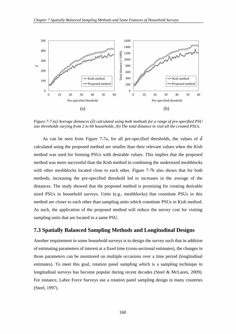
Chapter 7 Spatially Balanced Sampling Methods and Some Features of Household Surveys
160
Figure 7-7 (a) Average distances (��) calculated using both methods for a range of pre-specified PSU
size thresholds varying from 2 to 60 households. (b) The total distance to visit all the created PSUs.
As can be seen from Figure 7-7a, for all pre-specified thresholds, the values of ��
calculated using the proposed method are smaller than their relevant values when the Kish
method was used for forming PSUs with desirable values. This implies that the proposed
method was more successful than the Kish method in combining the undersized meshblocks
with other meshblocks located close to each other. Figure 7-7b also shows that for both
methods, increasing the pre-specified threshold led to increases in the average of the
distances. The study showed that the proposed method is promising for creating desirable
sized PSUs in household surveys. Units (e.g., meshblocks) that constitute PSUs in this
method are closer to each other than sampling units which constitute PSUs in Kish method.
As such, the application of the proposed method will reduce the survey cost for visiting
sampling units that are located in a same PSU.
7.3 Spatially Balanced Sampling Methods and Longitudinal Designs
Another requirement in some household surveys is to design the survey such that in addition
of estimating parameters of interest at a fixed time (cross-sectional estimates), the changes in
those parameters can be monitored on multiple occasions over a time period (longitudinal
estimates). To meet this goal, rotation panel sampling which is a sampling technique in
longitudinal surveys has become popular during recent decades (Steel & McLaren, 2009).
For instance, Labor Force Surveys use a rotation panel sampling design in many countries
(Steel, 1997).
0
200
400
600
800
1000
1200
1400
1600
0 10 20 30 40 50 60
To
tal
dis
tan
ce (
1000
)
Pre-specified threshold
Kish method
Proposed method
(b)
0
100
200
300
400
500
0 10 20 30 40 50 60
Pre-specified threshold
Kish method
Proposed method
(a)
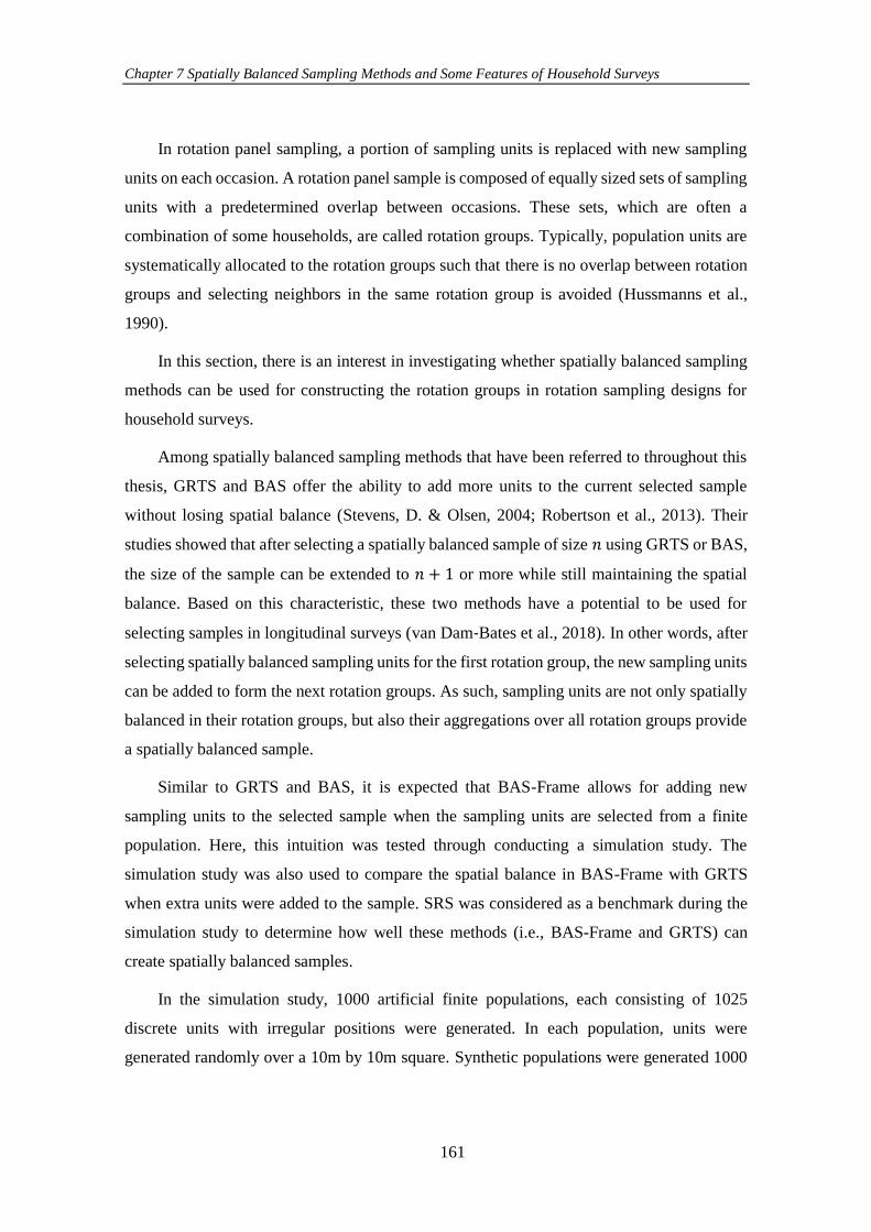
Chapter 7 Spatially Balanced Sampling Methods and Some Features of Household Surveys
161
In rotation panel sampling, a portion of sampling units is replaced with new sampling
units on each occasion. A rotation panel sample is composed of equally sized sets of sampling
units with a predetermined overlap between occasions. These sets, which are often a
combination of some households, are called rotation groups. Typically, population units are
systematically allocated to the rotation groups such that there is no overlap between rotation
groups and selecting neighbors in the same rotation group is avoided (Hussmanns et al.,
1990).
In this section, there is an interest in investigating whether spatially balanced sampling
methods can be used for constructing the rotation groups in rotation sampling designs for
household surveys.
Among spatially balanced sampling methods that have been referred to throughout this
thesis, GRTS and BAS offer the ability to add more units to the current selected sample
without losing spatial balance (Stevens, D. & Olsen, 2004; Robertson et al., 2013). Their
studies showed that after selecting a spatially balanced sample of size 𝑛 using GRTS or BAS,
the size of the sample can be extended to 𝑛 + 1 or more while still maintaining the spatial
balance. Based on this characteristic, these two methods have a potential to be used for
selecting samples in longitudinal surveys (van Dam‐Bates et al., 2018). In other words, after
selecting spatially balanced sampling units for the first rotation group, the new sampling units
can be added to form the next rotation groups. As such, sampling units are not only spatially
balanced in their rotation groups, but also their aggregations over all rotation groups provide
a spatially balanced sample.
Similar to GRTS and BAS, it is expected that BAS-Frame allows for adding new
sampling units to the selected sample when the sampling units are selected from a finite
population. Here, this intuition was tested through conducting a simulation study. The
simulation study was also used to compare the spatial balance in BAS-Frame with GRTS
when extra units were added to the sample. SRS was considered as a benchmark during the
simulation study to determine how well these methods (i.e., BAS-Frame and GRTS) can
create spatially balanced samples.
In the simulation study, 1000 artificial finite populations, each consisting of 1025
discrete units with irregular positions were generated. In each population, units were
generated randomly over a 10m by 10m square. Synthetic populations were generated 1000
Chapter 7 Spatially Balanced Sampling Methods and Some Features of Household Surveys
162
times to ensure that the results are reliable enough to represent the generated populations.
The size of the populations was set to 1025 units (210 + 1) to represent a worst case scenario
that needs to add extra units with zero inclusion probabilities.
From each population generated in this study (of size 1025 units), a sample of size 𝑛 =
2 units (the smallest sample size) was initially selected by each of the three sampling schemes
listed above. New units were then added to the sample one by one over time following reverse
hierarchical order for GRTS (Stevens, D. & Olsen, 2004) and Halton points sequence for
BAS-Frame. The process of adding sampling units was continued until a sampling fraction
equal to 50% of the population (512 sampling units) was achieved. The new units can be
added to the sample using different schemes (e.g., 5 by 5, 10 by 10, etc.); however, in this
study new units were added to the sample one by one. This will provide a basis to cover the
other schemes of adding different numbers of new units to the sample.
For each generated population, and in each step of adding a new unit to the sample, the
mean square error of sum of the inclusion probabilities of units in Voronoi polygons, ζ𝑖𝑛 (𝑖 =
1, … , 100 ; 𝑛 = 1,… ,512) explained in Equation (2.22), were calculated as a measure of
spatial balance. Then, the average of ζ𝑖𝑛 among 1000 generated populations (ζ𝑛) was
calculated.
The ratio of ζ𝑛 for GRTS and BAS-Frame when compared to SRS and each other are
plotted in Figure 7-8.
Figure 7-8 The ratio of 𝜁�� for GRTS, BAS-Frame when compared to SRS and each other for a situation when sampling units are added to the sample one by one over a period of time.
Chapter 7 Spatially Balanced Sampling Methods and Some Features of Household Surveys
163
Figure 7-8 shows, for all of the sample sizes considered in this study, the ratio of ζ𝑛 for
both the BAS-Frame technique and GRTS was less than 1 when compared with SRS. The
result associated with GRTS is in line with the previous studies (Stevens, D. & Olsen, 2004).
The study also showed that BAS-Frame created a more spatially balanced sample than SRS
when new sampling units were added to the sample. Although both techniques provided more
spatially balanced sample compared to SRS, the ratio of ζ𝑛 for GRTS is greater than ratio of
ζ𝑛 for BAS-Frame for all sample sizes. This means that the use of the BAS-Frame in adding
new units to the sample results in more spatially balanced samples.
Based on the results derived from the simulation study, it could be concluded that the
BAS-Frame method can be also employed in designing a rotation panel sample. This is
because the BAS-Frame can add new sampling units to the sample such that the cumulative
set of selected samples over the survey period is spatially balanced.
To implement BAS-Frame for creating rotation groups, after creating a long list of
Halton sequence, sampling units (based on the rotation group’s size) are selected (by the
BAS-Frame method) to form the first rotation group. Subsequently, new sampling units are
added to the sample to form the second rotation group. The process of adding new sampling
units to the sample is continued to create all the rotation groups. In this process, rotation
groups are created by tracing sequential points in the Halton sequence. Note that, Halton
points associated with the sampling units selected in the previous rotation groups are no
longer considered for the newly formed rotation groups.
Assuming that in a longitudinal sampling survey design, the 100 dwellings are required
to be allocated into 20 rotation groups, the first 5 dwellings selected by BAS-Frame are
considered as rotation group 1, the next 5 selected dwellings are considered as rotation group
2 and so on, and finally the last 5 selected dwellings are considered as rotation group 20. Note
that, for each rotation group, sampling dwellings are selected by continuing from the last-
used Halton point in the previous rotation group. Figure 7-9 illustrates the dwellings allocated
into 20 different rotation groups in a population consisted of 100 randomly generated
dwellings. Dwellings in the same rotation groups are shown in the same colour.
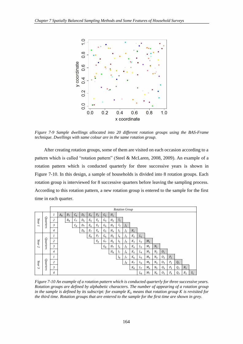
Chapter 7 Spatially Balanced Sampling Methods and Some Features of Household Surveys
164
Figure 7-9 Sample dwellings allocated into 20 different rotation groups using the BAS-Frame technique. Dwellings with same colour are in the same rotation group.
After creating rotation groups, some of them are visited on each occasion according to a
pattern which is called “rotation pattern” (Steel & McLaren, 2008, 2009). An example of a
rotation pattern which is conducted quarterly for three successive years is shown in
Figure 7-10. In this design, a sample of households is divided into 8 rotation groups. Each
rotation group is interviewed for 8 successive quarters before leaving the sampling process.
According to this rotation pattern, a new rotation group is entered to the sample for the first
time in each quarter.
Figure 7-10 An example of a rotation pattern which is conducted quarterly for three successive years.
Rotation groups are defined by alphabetic characters. The number of appearing of a rotation group
in the sample is defined by its subscript: for example 𝐾3 means that rotation group 𝐾 is revisited for
the third time. Rotation groups that are entered to the sample for the first time are shown in grey.
Rotation Group
Yea
r 1
Qu
arte
rs
1
2
3
4
Yea
r 2
Qu
arte
rs
1
2
3
4
Yea
r 3
Qu
arte
rs
1
2
3
4
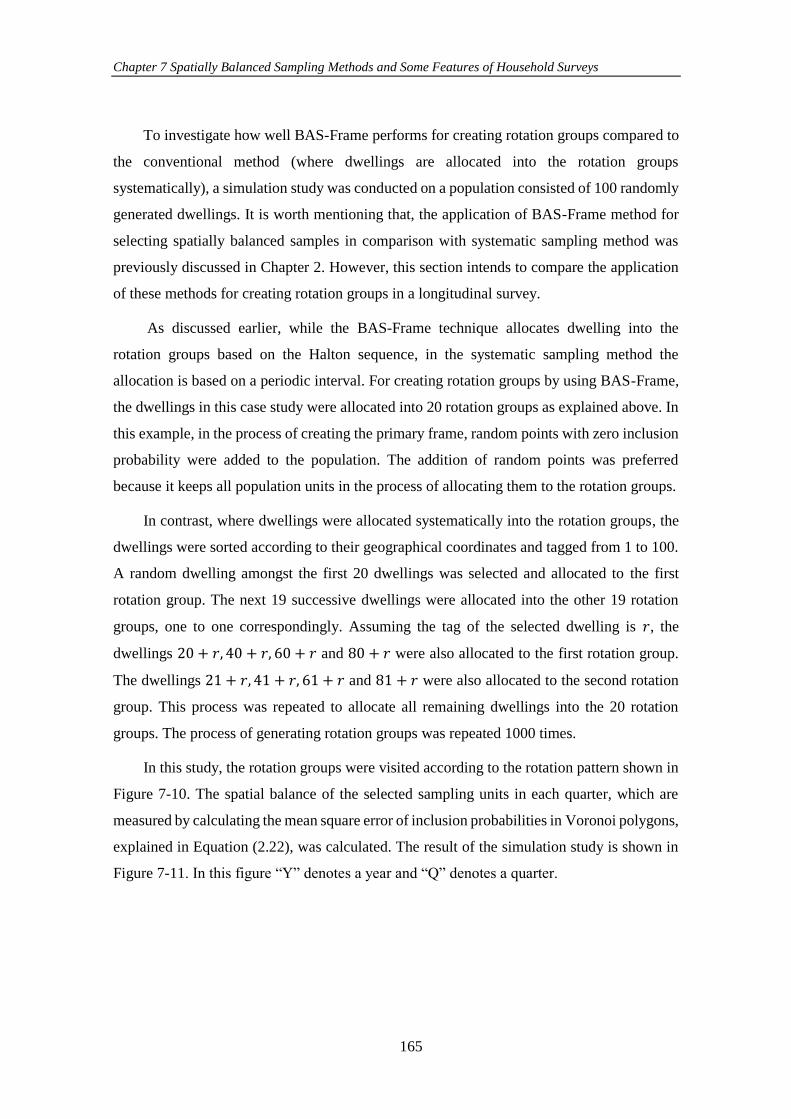
Chapter 7 Spatially Balanced Sampling Methods and Some Features of Household Surveys
165
To investigate how well BAS-Frame performs for creating rotation groups compared to
the conventional method (where dwellings are allocated into the rotation groups
systematically), a simulation study was conducted on a population consisted of 100 randomly
generated dwellings. It is worth mentioning that, the application of BAS-Frame method for
selecting spatially balanced samples in comparison with systematic sampling method was
previously discussed in Chapter 2. However, this section intends to compare the application
of these methods for creating rotation groups in a longitudinal survey.
As discussed earlier, while the BAS-Frame technique allocates dwelling into the
rotation groups based on the Halton sequence, in the systematic sampling method the
allocation is based on a periodic interval. For creating rotation groups by using BAS-Frame,
the dwellings in this case study were allocated into 20 rotation groups as explained above. In
this example, in the process of creating the primary frame, random points with zero inclusion
probability were added to the population. The addition of random points was preferred
because it keeps all population units in the process of allocating them to the rotation groups.
In contrast, where dwellings were allocated systematically into the rotation groups, the
dwellings were sorted according to their geographical coordinates and tagged from 1 to 100.
A random dwelling amongst the first 20 dwellings was selected and allocated to the first
rotation group. The next 19 successive dwellings were allocated into the other 19 rotation
groups, one to one correspondingly. Assuming the tag of the selected dwelling is 𝑟, the
dwellings 20 + 𝑟, 40 + 𝑟, 60 + 𝑟 and 80 + 𝑟 were also allocated to the first rotation group.
The dwellings 21 + 𝑟, 41 + 𝑟, 61 + 𝑟 and 81 + 𝑟 were also allocated to the second rotation
group. This process was repeated to allocate all remaining dwellings into the 20 rotation
groups. The process of generating rotation groups was repeated 1000 times.
In this study, the rotation groups were visited according to the rotation pattern shown in
Figure 7-10. The spatial balance of the selected sampling units in each quarter, which are
measured by calculating the mean square error of inclusion probabilities in Voronoi polygons,
explained in Equation (2.22), was calculated. The result of the simulation study is shown in
Figure 7-11. In this figure “Y” denotes a year and “Q” denotes a quarter.
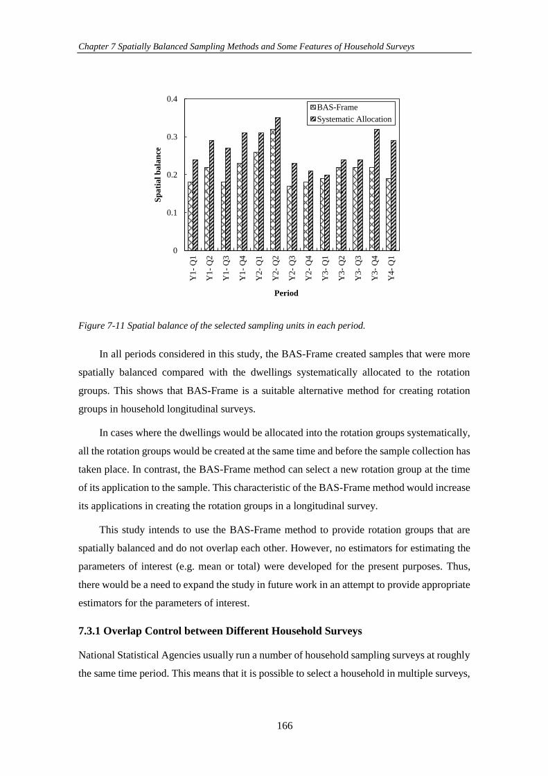
Chapter 7 Spatially Balanced Sampling Methods and Some Features of Household Surveys
166
Figure 7-11 Spatial balance of the selected sampling units in each period.
In all periods considered in this study, the BAS-Frame created samples that were more
spatially balanced compared with the dwellings systematically allocated to the rotation
groups. This shows that BAS-Frame is a suitable alternative method for creating rotation
groups in household longitudinal surveys.
In cases where the dwellings would be allocated into the rotation groups systematically,
all the rotation groups would be created at the same time and before the sample collection has
taken place. In contrast, the BAS-Frame method can select a new rotation group at the time
of its application to the sample. This characteristic of the BAS-Frame method would increase
its applications in creating the rotation groups in a longitudinal survey.
This study intends to use the BAS-Frame method to provide rotation groups that are
spatially balanced and do not overlap each other. However, no estimators for estimating the
parameters of interest (e.g. mean or total) were developed for the present purposes. Thus,
there would be a need to expand the study in future work in an attempt to provide appropriate
estimators for the parameters of interest.
7.3.1 Overlap Control between Different Household Surveys
National Statistical Agencies usually run a number of household sampling surveys at roughly
the same time period. This means that it is possible to select a household in multiple surveys,
0
0.1
0.2
0.3
0.4
Y1
- Q
1
Y1
- Q
2
Y1
- Q
3
Y1
- Q
4
Y2
- Q
1
Y2
- Q
2
Y2
- Q
3
Y2
- Q
4
Y3
- Q
1
Y3
- Q
2
Y3
- Q
3
Y3
- Q
4
Y4
- Q
1
Sp
ati
al
ba
lan
ce
Period
BAS-Frame
Systematic Allocation
Chapter 7 Spatially Balanced Sampling Methods and Some Features of Household Surveys
167
which will increase the undue respondent burden for that household. To reduce this burden,
it is usually desirable to avoid selecting the same unit for more than one survey, while
ensuring the units have their probabilities of selection for the survey to represent all of the
population. Various procedures have been developed to minimize overlap with later surveys.
A list of these procedures can be found in Ernst (1996, 1999), Chowdhury et al. (2000) and
Lu (2012). In these procedures, the inclusion probability for each population unit is
conditional on some aspect of its past usage to minimize the selection of units that have been
selected before.
It was discussed that (Section 7.3) the overlap between rotation groups can be controlled
by using the BAS-Frame method through discarding Halton points associated with the
sampling units selected in several rotation groups. Discarding such repeated Halton points
would result in selection of dependent samples. Such dependency is not desirable when it
comes to selecting independent samples amongst different surveys. As such, repeated Halton
points should not be discarded in the case of selecting independent samples. Therefore, the
surveys might overlap each other.
However, as the size of the population increases, the boxes in the BAS-Frame get
smaller. BAS points are spread evenly over the unit square, so when the BAS-Frame boxes
are small, it is unlikely that multiple BAS points are selected in the same box.
To show the advantage of using BAS-Frame in avoiding selecting same sampling units
for different surveys, a simulation study was conducted on the Christchurch meshblocks
dataset which contains 2684 meshblocks. In the simulation study, it was assumed that three
successive surveys (S1, S2 and S3) with three different sampling fractions (7%, 9% and 10%,
respectively) need to be implemented independently on Christchurch meshblocks. For each
survey, 1000 samples were selected using LPM, BAS-Frame and SRS method. After
completing the sample selection, the average number of meshblocks that repeated in
successive surveys was calculated. In both SRS and LPM, there was an average 4% overlap
between samples of successive surveys together, whereas using the BAS-Frame created an
average less than 1% overlap between successive surveys.
The results confirm the ability of the BAS-Frame method in conducting different
household surveys such that sampling units do not overlap each other. BAS-Frame provides
independent samples without making any change in the population units’ inclusion
Chapter 7 Spatially Balanced Sampling Methods and Some Features of Household Surveys
168
probabilities. This advantage of BAS-Frame highlights its potential application in providing
official statistics.
7.4 Spatially Balanced Sampling Methods and Availability of Auxiliary
Information in the Design Stage
Auxiliary information plays an important role in designing a sample for household surveys.
In cases where only one auxiliary variable, which is correlated with the response variable, is
available, it may be preferable to apply an unequal probability sampling method (i.e., PPS
sampling method) to select more representative sample. In this situation the auxiliary variable
is used as a measure of size of the population units. The application of spatially balanced
sampling methods for selecting unequal probability samples in the presence of one available
numerical auxiliary variable was shown in Section 6.2.1.
In cases with few qualitative auxiliary variables, these variables might be used in
stratifying the population into some homogenous strata and applying a stratified sampling
method to decrease the variance of population estimates. For instance, a stratified spatially
balanced sample may be obtained in the simplest way by taking a spatially balanced sample
in each stratum of the population separately. However, when there are many auxiliary
variables, the stratified sampling may become more complicated in terms of finding the
optimum number of strata and defining the strata boundaries. In these situations, instead of
stratifying the population, it could be useful to extend the rationale of the spatially balanced
sampling methods to spread the sample in the space of the auxiliary variables. In fact, it would
be of more interest to select a well-spread sample, not only over the geographical region of
the target population but also in the space of the auxiliary variables at the same time. LPMs
and BAS are two popular spatially balanced sampling methods that can select samples from
more than two-dimensions. As mentioned in Chapter 5, BAS-Frame can also select spatially
balanced samples from more than two dimensions. This subsection investigates the efficiency
of LPMs and BAS-Frame in spreading the sample in the space of available auxiliary variables
in household surveys.
7.4.1 The Principles of LPMs and BAS-Frame in Spreading the Samples Over the
Space of Auxiliary Variables
In a general format, the LPM methods select a sample by calculating distances (i.e., Euclidean
distance) between population units. In the presence of auxiliary variables, further to
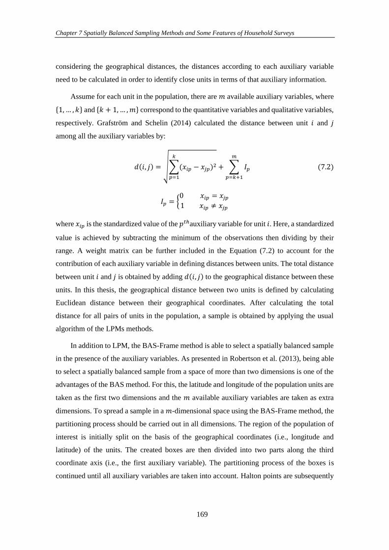
Chapter 7 Spatially Balanced Sampling Methods and Some Features of Household Surveys
169
considering the geographical distances, the distances according to each auxiliary variable
need to be calculated in order to identify close units in terms of that auxiliary information.
Assume for each unit in the population, there are 𝑚 available auxiliary variables, where
{1, … , 𝑘} and {𝑘 + 1,… ,𝑚} correspond to the quantitative variables and qualitative variables,
respectively. Grafström and Schelin (2014) calculated the distance between unit 𝑖 and 𝑗
among all the auxiliary variables by:
𝑑(𝑖, 𝑗) = √∑(𝑥𝑖𝑝 − 𝑥𝑗𝑝)2
𝑘
𝑝=1
+ ∑ 𝐼𝑝
𝑚
𝑝=𝑘+1
(7.2)
𝐼𝑝 = {0 𝑥𝑖𝑝 = 𝑥𝑗𝑝1 𝑥𝑖𝑝 ≠ 𝑥𝑗𝑝
where 𝑥𝑖𝑝 is the standardized value of the 𝑝𝑡ℎauxiliary variable for unit 𝑖. Here, a standardized
value is achieved by subtracting the minimum of the observations then dividing by their
range. A weight matrix can be further included in the Equation (7.2) to account for the
contribution of each auxiliary variable in defining distances between units. The total distance
between unit 𝑖 and 𝑗 is obtained by adding 𝑑(𝑖, 𝑗) to the geographical distance between these
units. In this thesis, the geographical distance between two units is defined by calculating
Euclidean distance between their geographical coordinates. After calculating the total
distance for all pairs of units in the population, a sample is obtained by applying the usual
algorithm of the LPMs methods.
In addition to LPM, the BAS-Frame method is able to select a spatially balanced sample
in the presence of the auxiliary variables. As presented in Robertson et al. (2013), being able
to select a spatially balanced sample from a space of more than two dimensions is one of the
advantages of the BAS method. For this, the latitude and longitude of the population units are
taken as the first two dimensions and the 𝑚 available auxiliary variables are taken as extra
dimensions. To spread a sample in a 𝑚-dimensional space using the BAS-Frame method, the
partitioning process should be carried out in all dimensions. The region of the population of
interest is initially split on the basis of the geographical coordinates (i.e., longitude and
latitude) of the units. The created boxes are then divided into two parts along the third
coordinate axis (i.e., the first auxiliary variable). The partitioning process of the boxes is
continued until all auxiliary variables are taken into account. Halton points are subsequently
Chapter 7 Spatially Balanced Sampling Methods and Some Features of Household Surveys
170
generated in (2 + 𝑚) dimensions (two geographical dimensions along with 𝑚 auxiliary
variables). A unit is selected as a sampling unit if its corresponding box in the primary frame
includes the generated Halton points in all dimensions. Note that, partitioning process may
not be directly applied for the categorical auxiliary variables as they need to be firstly
represented by numerical variables with jittered values. As such, in this study the BAS-Frame
method has not been employed for spreading sampling units over the space of categorical
auxiliary variables.
To investigate the possibility of using BAS-Frame in selecting a representative sample
in the presence of auxiliary variables and compare it with LPM, a simulation study was
performed on the Baltimore data set (Dubin, 1992). This dataset contains the selling price as
well as other attributes related to 211 housing units. In this simulation study the “selling price
in thousands of dollars (Price)” was considered as the response variable. In addition to
geographical coordinates related to each house, three variables “Number of rooms
(Nrooms)”, “Age of dwelling, in years (Age)” and “Lot size, in hundreds of square feet
(Lotsz)” were also considered as auxiliary variables.
A total of 1000 samples of sizes 10, 15, 20 and 25 out of 211 were selected by LPM and
BAS-Frame. SRS was also considered in order to make a comparison between different
designs. In this example, population units were assigned an equal probability of selection. As
such, the primary frame required in the BAS-Frame method was created by removing points
randomly from the population (as discussed in Chapter 5, when samples are selected by equal
probability of selection, removing random points during the partitioning process results in
more spatially balanced samples compare to a situation that random points are added to the
population). By using LPM and BAS-Frame, we aim to spread the sampling units not only
over the geographical region of the population of houses, but also over the space created by
the three auxiliary variables to ensure that each considered auxiliary variable will be
represented in the sample.
Similarly to other simulation studies implemented throughout this thesis, after defining
Voronoi polygons related to each sampling units, the ζ explained in Equation (2.22) was used
as an index for measuring how well spread the selected samples were. But, here, in addition
to geographical distance between sampling units, the auxiliary distances between sampling
units were considered for defining each Voronoi polygon. In fact, the ζ was calculated in five
dimensions (two geographical dimensions and three auxiliary variables). Here, the “sb”

Chapter 7 Spatially Balanced Sampling Methods and Some Features of Household Surveys
171
function available in “Balanced Sampling” package in R was used for calculating ζ. After
selecting the 1000 samples, the average of spatial balance, ζ , was calculated for each
sampling method. The results of the simulation study are reported in Table 7-3.
Table 7-3 The average of 𝜁 among 1000 iterations for BAS-Frame and LPM in comparison with the
relevant value for SRS.
Sample
size
Design
BAS-Frame / SRS LPM / SRS
10 0.51 0.49
15 0.54 0.49
20 0.56 0.49
25 0.63 0.50
As can be seen from Table 7-3, the ratio of 𝜁 for both LPM and BAS-Frame in
comparison to SRS is less than 1. This shows that these two methods spread samples more
evenly over the region of population than SRS. To find out how representative the selected
samples are, the distribution of sample means for each auxiliary variable was compared with
its population distribution. The distribution of the sample mean of the auxiliary variables
based on 1000 samples of size 10 for different sampling methods are presented in Figure 7-12.
The true average value of each auxiliary variable in the population (5.2 for Nrooms, 30.1 for
Age, and 72.3 for Lotsz) is also defined by vertical dash lines in its relevant distribution.
Figure 7-12 shows that the sampling distributions obtained by all the three methods
encompass the true values of parameters in the population.
The variance of the total estimation of the target variable (Price) and the other auxiliary
variables (Nroom, Age and Lotsz) was also simulated using the simulated variance estimator
in Equation (5.3). The simulated variances of the variables of interest for LPM and BAS-
Frame in relation to SRS for four different sample sizes are shown in Table 7-4.
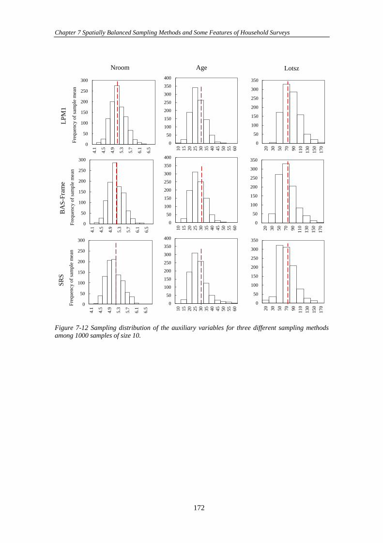
Chapter 7 Spatially Balanced Sampling Methods and Some Features of Household Surveys
172
Figure 7-12 Sampling distribution of the auxiliary variables for three different sampling methods among 1000 samples of size 10.
LP
M1
Nroom Age LotszB
AS
-Fra
me
SR
S
0
50
100
150
200
250
300
4.1
4.5
4.9
5.3
5.7
6.1
6.5
Fre
qu
ency
of
sam
ple
mea
n
0
50
100
150
200
250
300
4.1
4.5
4.9
5.3
5.7
6.1
6.5
Fre
qu
ency
of
sam
ple
mea
n
0
50
100
150
200
250
300
350
20
30
50
70
90
11
0
13
0
15
0
17
0
0
50
100
150
200
250
300
4.1
4.5
4.9
5.3
5.7
6.1
6.5
Fre
qu
ency
of
sam
ple
mea
n
0
50
100
150
200
250
300
350
400
10
15
20
25
30
35
40
45
50
55
60
0
50
100
150
200
250
300
350
20
30
50
70
90
11
0
13
0
15
0
17
0
0
50
100
150
200
250
300
350
400
10
15
20
25
30
35
40
45
50
55
60
0
50
100
150
200
250
300
350
400
10
15
20
25
30
35
40
45
50
55
60
0
50
100
150
200
250
300
350
20
30
50
70
90
11
0
130
150
170
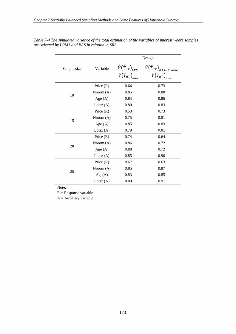
Chapter 7 Spatially Balanced Sampling Methods and Some Features of Household Surveys
173
Table 7-4 The simulated variance of the total estimation of the variables of interest where samples
are selected by LPM1 and BAS in relation to SRS.
Sample size Variable
Design
��(��𝐻𝑇)𝐿𝑃𝑀��(��𝐻𝑇)𝑆𝑅𝑆
��(��𝐻𝑇)𝐵𝐴𝑆−𝐹𝑟𝑎𝑚𝑒
��(��𝐻𝑇)𝑆𝑅𝑆
10
Price (R) 0.64 0.73
Nroom (A) 0.85 0.88
Age (A) 0.84 0.86
Lotsz (A) 0.80 0.83
15
Price (R) 0.53 0.73
Nroom (A) 0.75 0.81
Age (A) 0.85 0.83
Lotsz (A) 0.79 0.81
20
Price (R) 0.74 0.64
Nroom (A) 0.86 0.72
Age (A) 0.88 0.72
Lotsz (A) 0.85 0.90
25
Price (R) 0.67 0.63
Nroom (A) 0.85 0.87
Age(A) 0.83 0.85
Lotsz (A) 0.89 0.91
Note:
R = Response variable
A = Auxiliary variable
Chapter 7 Spatially Balanced Sampling Methods and Some Features of Household Surveys
174
Table 7-4 shows that both LPM and BAS-Frame have smaller simulated variance in
estimating the response variable (Price) than SRS when the sampling units are spread not
only according to their geographical locations, but also when they are spread over the space
of auxiliary variables (two geographical dimensions and three auxiliary variables). Results
also showed that spreading the sampling units over the space of the auxiliary variables by
using spatially balanced sampling methods provided smaller simulated variance for
estimating each auxiliary variable (total of Nroom, Age and Lotsz). Note that, the effect of
considering auxiliary variables as stratification variables has been previously investigated in
Section 5.4.
7.4.2 Efficiency of BAS-Frame and Number of Auxiliary Variables
There are studies available in the literature that indicate some correlation between points
generated in Halton sequences for higher primes (Hess & Polak, 2003; Vandewoestyne &
Cools, 2006; Schlier, 2008). For example, the first 10 pairs of points generated by the primes
11 and 13: (1 11⁄ , 1 13⁄ ), (2 11⁄ , 2 13⁄ ), … , (10 11⁄ , 10 13⁄ ), have a linear correlation.
Helpful displays showing the correlation between dimensions of Halton sequences for higher
primes can be found in Chi et al. (2005) and Vandewoestyne and Cools (2006). Correlation
between Halton points in higher dimensions may deteriorate the performance of the Halton
sequence in generating evenly spread points over an interval. Therefore, it can be concluded
that the BAS-Frame method may fail to generate a well-spread sample in the presence of a
large number of auxiliary variables. This is shown here through conducting a simulation study
on Christchurch meshblocks. In the simulation study, in addition to longitude and latitude of
meshblocks, the ten variables listed below were considered as auxiliary variables:
male: number of males,
female : number of females,
Māori: number of Māori,
child: number of people who are 0 to 14 years old,
young: number of people who are 15 to 64 years old,
adult: number of people who are more than 65 years old,
unemployed: number of unemployed people,
employed: number of employed people,
one-storey: number of one-storey housing units,
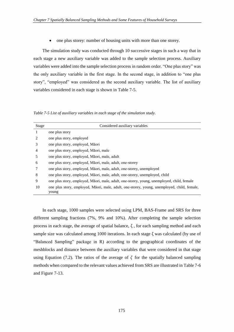
Chapter 7 Spatially Balanced Sampling Methods and Some Features of Household Surveys
175
one plus storey: number of housing units with more than one storey.
The simulation study was conducted through 10 successive stages in such a way that in
each stage a new auxiliary variable was added to the sample selection process. Auxiliary
variables were added into the sample selection process in random order. “One plus story” was
the only auxiliary variable in the first stage. In the second stage, in addition to “one plus
story”, “employed” was considered as the second auxiliary variable. The list of auxiliary
variables considered in each stage is shown in Table 7-5.
Table 7-5 List of auxiliary variables in each stage of the simulation study.
Stage Considered auxiliary variables
1 one plus story
2 one plus story, employed
3 one plus story, employed, Māori
4 one plus story, employed, Māori, male
5 one plus story, employed, Māori, male, adult
6 one plus story, employed, Māori, male, adult, one-storey
7 one plus story, employed, Māori, male, adult, one-storey, unemployed
8 one plus story, employed, Māori, male, adult, one-storey, unemployed, child
9 one plus story, employed, Māori, male, adult, one-storey, young, unemployed, child, female
10 one plus story, employed, Māori, male, adult, one-storey, young, unemployed, child, female,
young
In each stage, 1000 samples were selected using LPM, BAS-Frame and SRS for three
different sampling fractions (7%, 9% and 10%). After completing the sample selection
process in each stage, the average of spatial balance, ζ , for each sampling method and each
sample size was calculated among 1000 iterations. In each stage ζ was calculated (by use of
“Balanced Sampling” package in R) according to the geographical coordinates of the
meshblocks and distance between the auxiliary variables that were considered in that stage
using Equation (7.2). The ratios of the average of 𝜁 for the spatially balanced sampling
methods when compared to the relevant values achieved from SRS are illustrated in Table 7-6
and Figure 7-13.
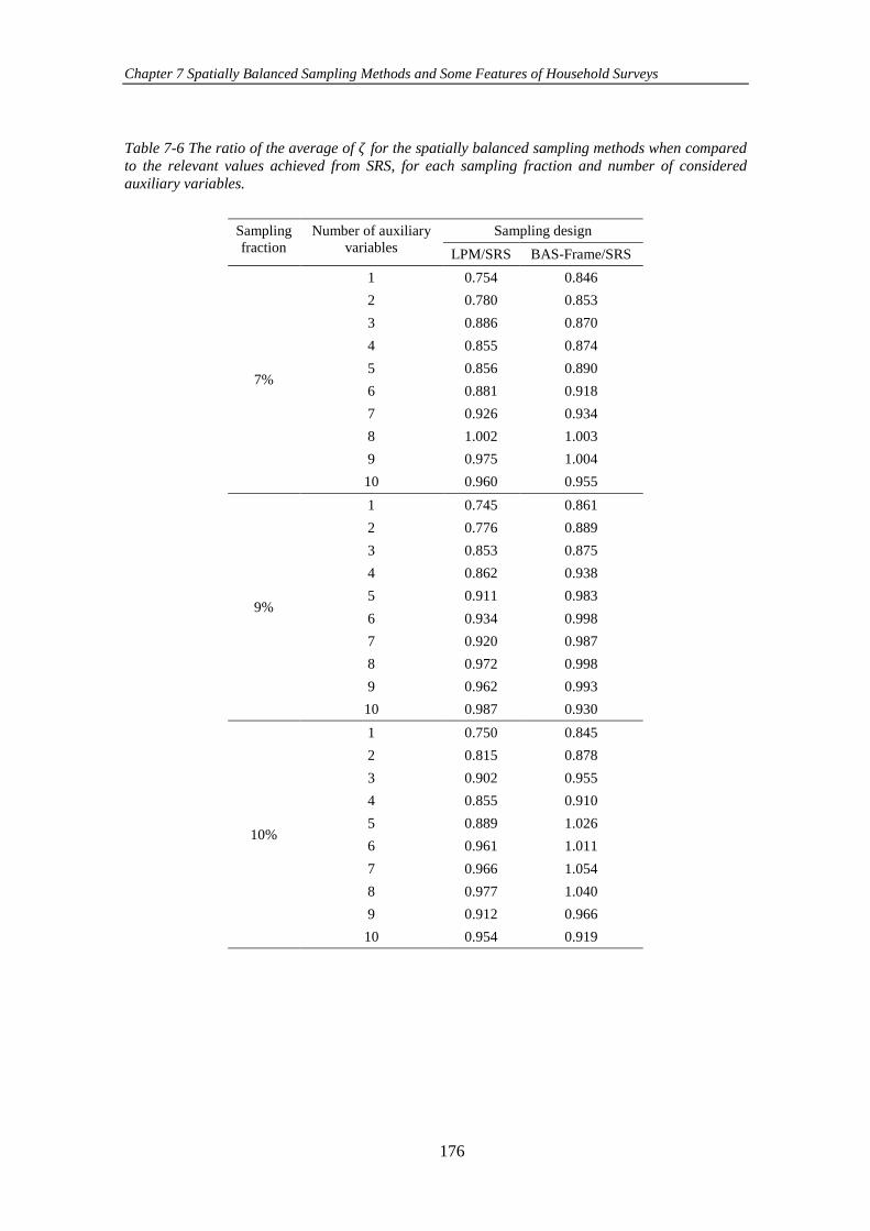
Chapter 7 Spatially Balanced Sampling Methods and Some Features of Household Surveys
176
Table 7-6 The ratio of the average of 𝜁 for the spatially balanced sampling methods when compared
to the relevant values achieved from SRS, for each sampling fraction and number of considered
auxiliary variables.
Sampling
fraction
Number of auxiliary
variables
Sampling design
LPM/SRS BAS-Frame/SRS
7%
1 0.754 0.846
2 0.780 0.853
3 0.886 0.870
4 0.855 0.874
5 0.856 0.890
6 0.881 0.918
7 0.926 0.934
8 1.002 1.003
9 0.975 1.004
10 0.960 0.955
9%
1 0.745 0.861
2 0.776 0.889
3 0.853 0.875
4 0.862 0.938
5 0.911 0.983
6 0.934 0.998
7 0.920 0.987
8 0.972 0.998
9 0.962 0.993
10 0.987 0.930
10%
1 0.750 0.845
2 0.815 0.878
3 0.902 0.955
4 0.855 0.910
5 0.889 1.026
6 0.961 1.011
7 0.966 1.054
8 0.977 1.040
9 0.912 0.966
10 0.954 0.919
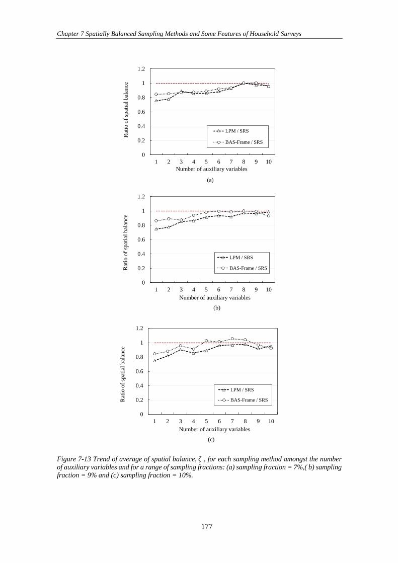
Chapter 7 Spatially Balanced Sampling Methods and Some Features of Household Surveys
177
Figure 7-13 Trend of average of spatial balance, 𝜁 , for each sampling method amongst the number
of auxiliary variables and for a range of sampling fractions: (a) sampling fraction = 7%,( b) sampling fraction = 9% and (c) sampling fraction = 10%.
(a)
0
0.2
0.4
0.6
0.8
1
1.2
1 2 3 4 5 6 7 8 9 10
Rat
io o
f sp
atia
l b
alan
ce
Number of auxiliary variables
LPM / SRS
BAS-Frame / SRS
(b)
0
0.2
0.4
0.6
0.8
1
1.2
1 2 3 4 5 6 7 8 9 10
Rat
io o
f sp
atia
l b
alan
ce
Number of auxiliary variables
LPM / SRS
BAS-Frame / SRS
(c)
0
0.2
0.4
0.6
0.8
1
1.2
1 2 3 4 5 6 7 8 9 10
Rat
io o
f sp
atia
l b
alan
ce
Number of auxiliary variables
LPM / SRS
BAS-Frame / SRS
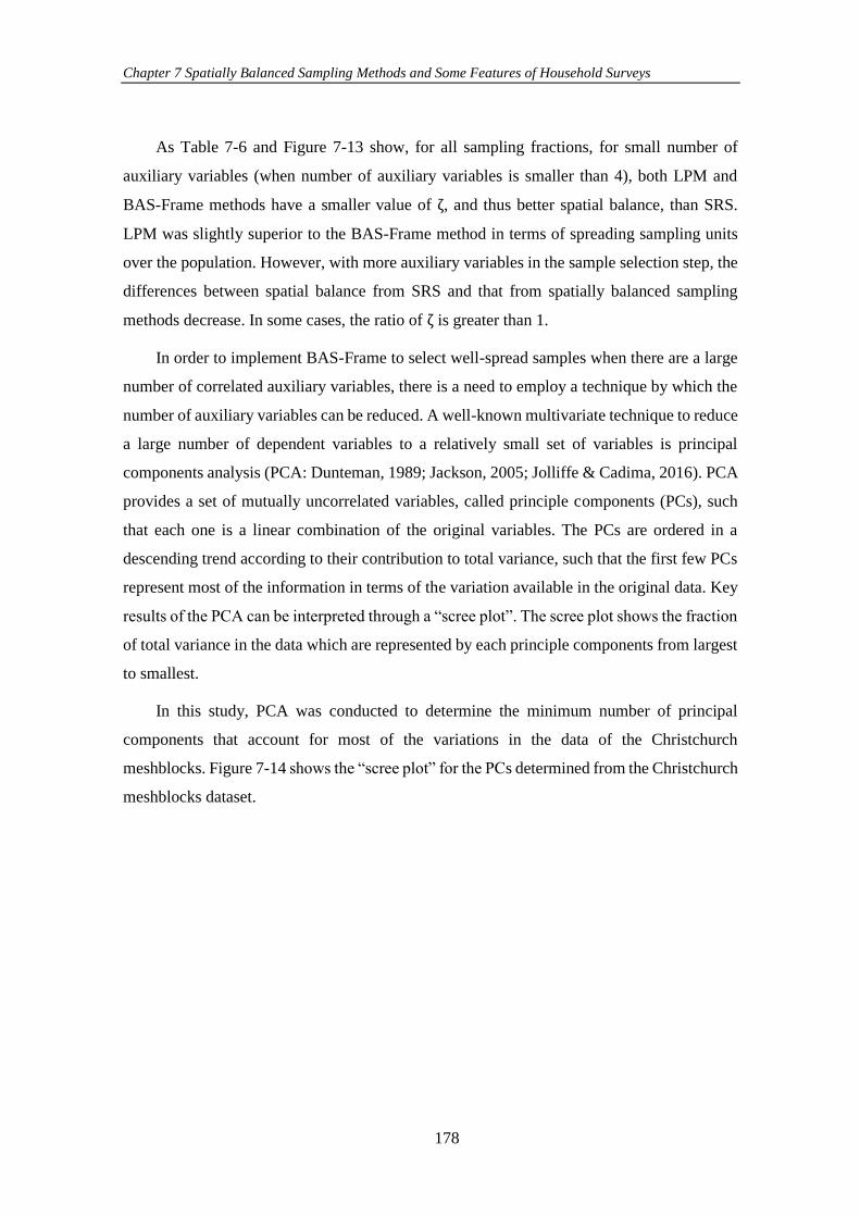
Chapter 7 Spatially Balanced Sampling Methods and Some Features of Household Surveys
178
As Table 7-6 and Figure 7-13 show, for all sampling fractions, for small number of
auxiliary variables (when number of auxiliary variables is smaller than 4), both LPM and
BAS-Frame methods have a smaller value of ζ, and thus better spatial balance, than SRS.
LPM was slightly superior to the BAS-Frame method in terms of spreading sampling units
over the population. However, with more auxiliary variables in the sample selection step, the
differences between spatial balance from SRS and that from spatially balanced sampling
methods decrease. In some cases, the ratio of ζ is greater than 1.
In order to implement BAS-Frame to select well-spread samples when there are a large
number of correlated auxiliary variables, there is a need to employ a technique by which the
number of auxiliary variables can be reduced. A well-known multivariate technique to reduce
a large number of dependent variables to a relatively small set of variables is principal
components analysis (PCA: Dunteman, 1989; Jackson, 2005; Jolliffe & Cadima, 2016). PCA
provides a set of mutually uncorrelated variables, called principle components (PCs), such
that each one is a linear combination of the original variables. The PCs are ordered in a
descending trend according to their contribution to total variance, such that the first few PCs
represent most of the information in terms of the variation available in the original data. Key
results of the PCA can be interpreted through a “scree plot”. The scree plot shows the fraction
of total variance in the data which are represented by each principle components from largest
to smallest.
In this study, PCA was conducted to determine the minimum number of principal
components that account for most of the variations in the data of the Christchurch
meshblocks. Figure 7-14 shows the “scree plot” for the PCs determined from the Christchurch
meshblocks dataset.
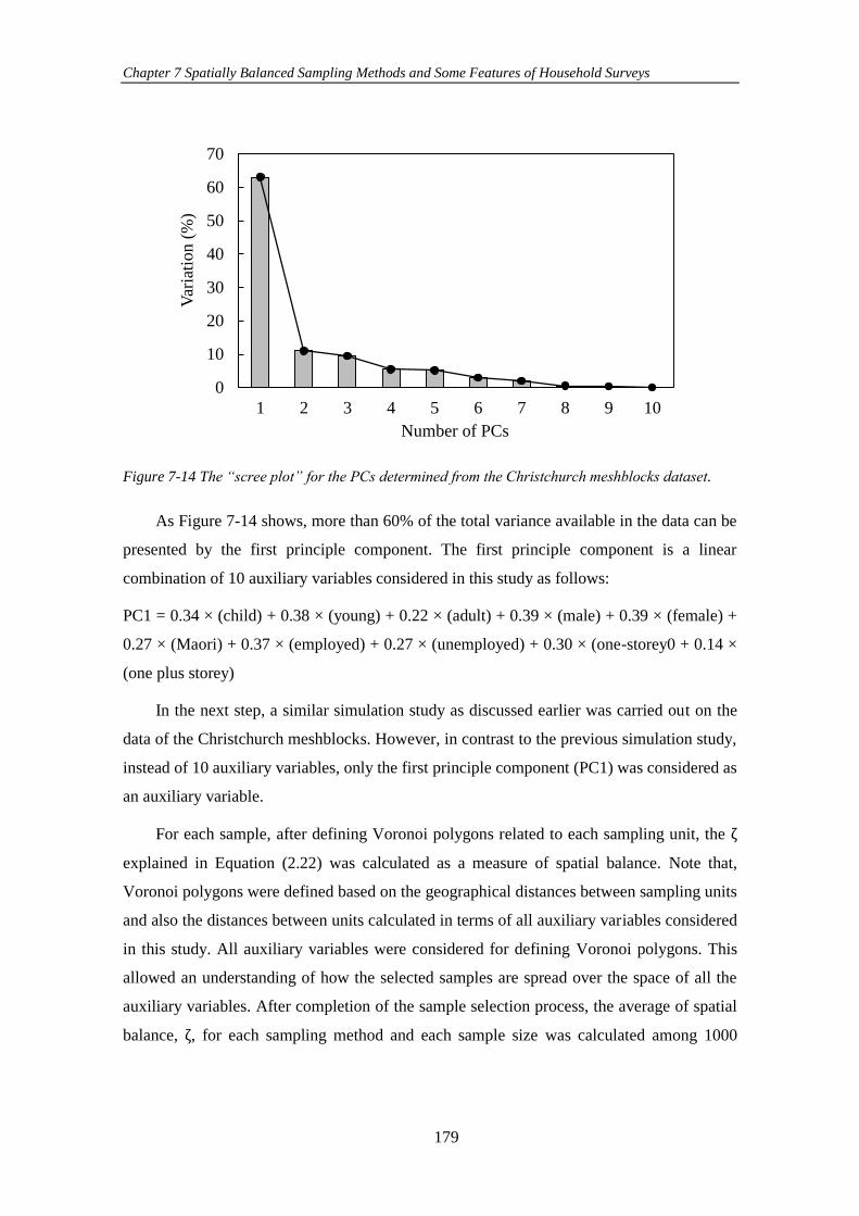
Chapter 7 Spatially Balanced Sampling Methods and Some Features of Household Surveys
179
Figure 7-14 The “scree plot” for the PCs determined from the Christchurch meshblocks dataset.
As Figure 7-14 shows, more than 60% of the total variance available in the data can be
presented by the first principle component. The first principle component is a linear
combination of 10 auxiliary variables considered in this study as follows:
PC1 = 0.34 × (child) + 0.38 × (young) + 0.22 × (adult) + 0.39 × (male) + 0.39 × (female) +
0.27 × (Maori) + 0.37 × (employed) + 0.27 × (unemployed) + 0.30 × (one-storey0 + 0.14 ×
(one plus storey)
In the next step, a similar simulation study as discussed earlier was carried out on the
data of the Christchurch meshblocks. However, in contrast to the previous simulation study,
instead of 10 auxiliary variables, only the first principle component (PC1) was considered as
an auxiliary variable.
For each sample, after defining Voronoi polygons related to each sampling unit, the ζ
explained in Equation (2.22) was calculated as a measure of spatial balance. Note that,
Voronoi polygons were defined based on the geographical distances between sampling units
and also the distances between units calculated in terms of all auxiliary variables considered
in this study. All auxiliary variables were considered for defining Voronoi polygons. This
allowed an understanding of how the selected samples are spread over the space of all the
auxiliary variables. After completion of the sample selection process, the average of spatial
balance, ζ, for each sampling method and each sample size was calculated among 1000
0
10
20
30
40
50
60
70
1 2 3 4 5 6 7 8 9 10
Var
iati
on (
%)
Number of PCs
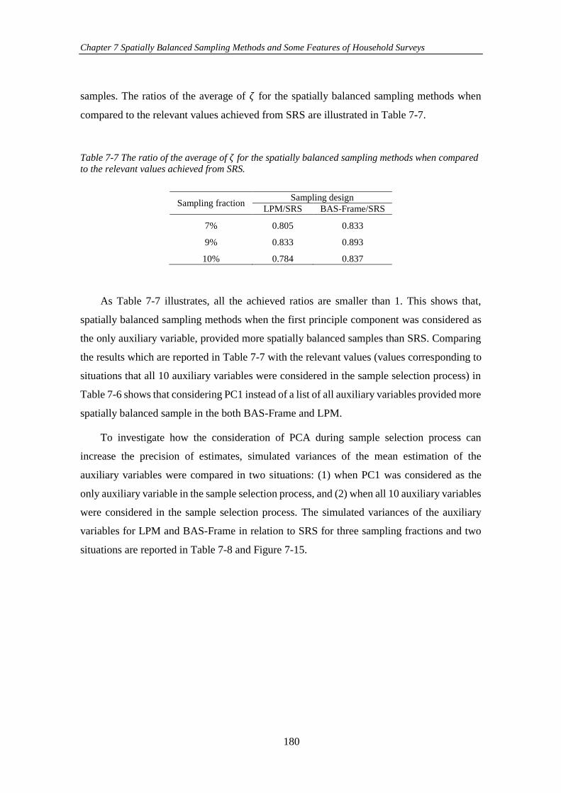
Chapter 7 Spatially Balanced Sampling Methods and Some Features of Household Surveys
180
samples. The ratios of the average of 𝜁 for the spatially balanced sampling methods when
compared to the relevant values achieved from SRS are illustrated in Table 7-7.
Table 7-7 The ratio of the average of 𝜁 for the spatially balanced sampling methods when compared to the relevant values achieved from SRS.
Sampling fraction Sampling design
LPM/SRS BAS-Frame/SRS
7% 0.805 0.833
9% 0.833 0.893
10% 0.784 0.837
As Table 7-7 illustrates, all the achieved ratios are smaller than 1. This shows that,
spatially balanced sampling methods when the first principle component was considered as
the only auxiliary variable, provided more spatially balanced samples than SRS. Comparing
the results which are reported in Table 7-7 with the relevant values (values corresponding to
situations that all 10 auxiliary variables were considered in the sample selection process) in
Table 7-6 shows that considering PC1 instead of a list of all auxiliary variables provided more
spatially balanced sample in the both BAS-Frame and LPM.
To investigate how the consideration of PCA during sample selection process can
increase the precision of estimates, simulated variances of the mean estimation of the
auxiliary variables were compared in two situations: (1) when PC1 was considered as the
only auxiliary variable in the sample selection process, and (2) when all 10 auxiliary variables
were considered in the sample selection process. The simulated variances of the auxiliary
variables for LPM and BAS-Frame in relation to SRS for three sampling fractions and two
situations are reported in Table 7-8 and Figure 7-15.
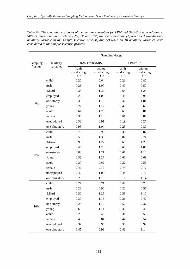
Chapter 7 Spatially Balanced Sampling Methods and Some Features of Household Surveys
181
Table 7-8 The simulated variances of the auxiliary variables for LPM and BAS-Frame in relation to
SRS for three sampling fractions (7%, 9% and 10%) and two situations: (1) when PC1 was the only
auxiliary variable in the sample selection process, and (2) when all 10 auxiliary variables were considered in the sample selection process.
Sampling
fraction
auxiliary
variables
Sampling design
BAS-Frame/SRS LPM/SRS
With
conducting
PCA
without
conducting
PCA
With
conducting
PCA
without
conducting
PCA
7%
child 0.20 0.64 0.21 0.80
male 0.26 1.00 0.40 0.50
Māori 0.35 1.34 0.65 1.25
employed 0.20 1.03 0.48 0.95
one-storey 0.30 1.19 0.42 1.04
young 0.22 1.12 0.46 0.60
adult 0.64 1.23 0.65 0.81
female 0.35 1.13 0.61 0.87
unemployed 0.38 0.91 0.19 0.27
one plus story 0.93 1.04 0.23 0.80
9%
child 0.72 0.92 0.38 0.87
male 0.53 1.38 0.82 0.74
Māori 0.93 1.27 0.69 1.28
employed 0.46 1.28 0.65 1.06
one-storey 0.83 1.21 0.61 1.10
young 0.55 1.27 0.60 0.69
adult 0.27 0.62 0.22 0.55
female 0.43 0.78 0.74 0.77
unemployed 0.40 1.06 0.44 0.72
one plus story 0.28 1.18 0.18 1.14
10%
child 0.27 0.71 0.42 0.70
male 0.23 0.90 0.20 0.55
Māori 0.50 1.25 0.58 1.17
employed 0.39 1.13 0.26 0.47
one-storey 0.24 1.12 0.59 0.37
young 0.65 1.14 0.39 0.42
adult 0.28 0.43 0.31 0.58
female 0.43 0.84 0.44 0.54
unemployed 0.37 0.95 0.35 0.92
one plus story 0.45 0.98 0.41 1.14
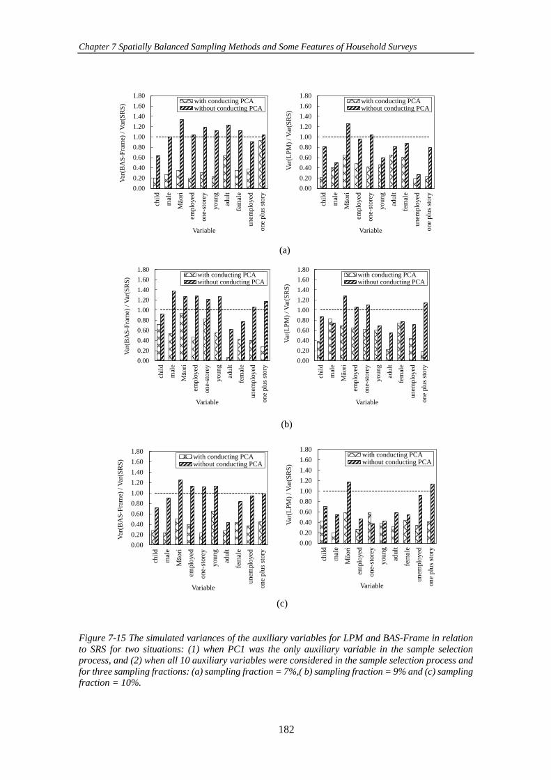
Chapter 7 Spatially Balanced Sampling Methods and Some Features of Household Surveys
182
Figure 7-15 The simulated variances of the auxiliary variables for LPM and BAS-Frame in relation
to SRS for two situations: (1) when PC1 was the only auxiliary variable in the sample selection process, and (2) when all 10 auxiliary variables were considered in the sample selection process and
for three sampling fractions: (a) sampling fraction = 7%,( b) sampling fraction = 9% and (c) sampling fraction = 10%.
(a)
0.00
0.20
0.40
0.60
0.80
1.00
1.20
1.40
1.60
1.80
chil
d
mal
e
Māori
emplo
yed
on
e-st
ore
y
yo
ung
adult
fem
ale
un
emp
loy
ed
on
e plu
s st
ory
Var
(BA
S-F
ram
e) /
Var
(SR
S)
Variable
with conducting PCAwithout conducting PCA
0.00
0.20
0.40
0.60
0.80
1.00
1.20
1.40
1.60
1.80
chil
d
mal
e
Māori
emplo
yed
on
e-st
ore
y
yo
ung
adult
fem
ale
un
emp
loy
ed
on
e plu
s st
ory
Var
(LP
M)
/ V
ar(S
RS
)
Variable
with conducting PCAwithout conducting PCA
(b)
0.00
0.20
0.40
0.60
0.80
1.00
1.20
1.40
1.60
1.80
chil
d
mal
e
Māori
emplo
yed
on
e-st
ore
y
yo
ung
adult
fem
ale
un
emp
loy
ed
on
e plu
s st
ory
Var
(BA
S-F
ram
e) /
Var
(SR
S)
Variable
with conducting PCAwithout conducting PCA
0.00
0.20
0.40
0.60
0.80
1.00
1.20
1.40
1.60
1.80
chil
d
mal
e
Māori
emplo
yed
on
e-st
ore
y
yo
ung
adult
fem
ale
un
emp
loy
ed
on
e plu
s st
ory
Var
(LP
M)
/ V
ar(S
RS
)
Variable
with conducting PCAwithout conducting PCA
(c)
0.00
0.20
0.40
0.60
0.80
1.00
1.20
1.40
1.60
1.80
chil
d
mal
e
Māori
emplo
yed
on
e-st
ore
y
yo
ung
adult
fem
ale
un
emp
loy
ed
on
e plu
s st
ory
Var
(BA
S-F
ram
e) /
Var
(SR
S)
Variable
with conducting PCAwithout conducting PCA
0.00
0.20
0.40
0.60
0.80
1.00
1.20
1.40
1.60
1.80
chil
d
mal
e
Māori
emplo
yed
on
e-st
ore
y
yo
ung
adult
fem
ale
un
emp
loy
ed
on
e plu
s st
ory
Var
(LP
M)
/ V
ar(S
RS
)
Variable
with conducting PCAwithout conducting PCA
Chapter 7 Spatially Balanced Sampling Methods and Some Features of Household Surveys
183
As Table 7-8 and Figure 7-15 show for all the auxiliary variables, the ratios of the simulated
variances for both LPM and BAS-Frame in comparison to SRS are less than 1 when PC1 was
considered as the only auxiliary variable. When PCA is included in the sample selection
process, these ratios are smaller than ratios corresponding to the situation that PCA was not
considered. Results confirmed that considering PC1 as the only auxiliary variable in the
sample selection process provided smaller simulated variance for estimating each of the
auxiliary variables.
The studies presented in this section showed that BAS-Frame can work as well as LPM in
terms of spreading the samples over the geographical region of the population and the space
of the auxiliary variables. The first principle component (PC1) was considered as the only
auxiliary variable because it explained more than 60% of the total variance available in the
data. However, in general, the number of required PCs is likely to vary in different situations
and should be determined using the “scree” plot.
7.5 Conclusions
The feasibility of applying spatially balanced sampling methods for dealing with some
common features of household sampling surveys was investigated in this chapter.
Combining undersized units in order to define PSUs with desirable sizes is one of the
features of household surveys studied in the first section. A famous method recommended by
the United Nations for constructing PSUs in developing country is the Kish method. Although
this method is easy to implement, it does not guarantee that the created PSUs include the
neighbouring units. In this chapter, a new technique for combining undersized units based on
the rationale of the BAS-Frame method was introduced. The performance of this technique
in terms of combining nearby units to form a PSU with a desirable size was compared with
the performance of the Kish method through running a simulation study. Results of the
simulation study showed that for all considered thresholds for defining PSUs, the average of
distances between combined units (calculated using the travelling salesman problem) in the
new technique was shorter than the distances between units combined together by the Kish
method.
Available literatures show that BAS and GRTS are able to add new sampling units to
the current sample, while keeping the spatial balance (Stevens, D. & Olsen, 2004; Robertson
Robertson et al., 2013). This study showed that such beneficial characteristic can also be
Chapter 7 Spatially Balanced Sampling Methods and Some Features of Household Surveys
184
accomplished using BAS-Frame. This feature of the BAS-Frame method makes it suitable
for longitudinal designs. It is likely that the same households or PSUs would be selected in
different household surveys when BAS-Frame is employed; however, as discussed, by
increasing the size of the population the overlap between successive surveys is expected to
be decreased.
The application of the BAS-Frame method in the presence of auxiliary variables was
studied in the last section. The study showed that when there are a small number of auxiliary
variables, the BAS-Frame method is able to spread the sampling units not only over the
geographical space of the population, but also over the space of the auxiliary variables.
However, its performance in spreading a sample over the space of the auxiliary variables
decreases as the number of auxiliary variables is increased. Principle component analysis was
used to reduce the number of correlated auxiliary variables.
After defining the required number of principle components (PCs) that explain an
acceptable percentage of the variation in the data (in this study 60% of the variation of the
data was explained by PC1), BAS-Frame method was employed to select samples according
to the selected PCs instead of considering all the auxiliary variables. The results showed that
the selected samples were more spatially balanced than the situation where all the auxiliary
variables were considered in the sample selection process.
7.6 References
Chi, H., Mascagni, M., & Warnock, T. (2005). On the optimal Halton sequence. Mathematics and
computers in Simulation, 70(1), 9-21.
Chowdhury, S., Chu, A., & Kaufman, S. (2000). Minimizing overlap in NCES surveys.
Proceedings of the Survey Methods Research Section. American Statistical Association,
174-179.
Dubin, R. A. (1992). Spatial autocorrelation and neighborhood quality. Regional science and
urban economics, 22(3), 433-452.
Dunteman, G. H. (1989). Principal components analysis: Sage.
Ernst, L. R. (1996). Maximizing the overlap of sample units for two designs with simultaneous
selection. Journal of Official Statistics, 12(1), 33.
Ernst, L. R. (1999). The maximization and minimization of sample overlap problems: a half
century of results. Paper presented at the Bulletin of the International Statistical Institute,
Proceedings.
Grafström, A., & Schelin, L. (2014). How to select representative samples. Scandinavian Journal
of Statistics, 41(2), 277-290.
Chapter 7 Spatially Balanced Sampling Methods and Some Features of Household Surveys
185
Hahsler, M., & Hornik, K. (2007). TSP-Infrastructure for the traveling salesperson problem.
Journal of Statistical Software, 23(2), 1-21.
Hess, S., & Polak, J. (2003). An alternative method to the scrambled Halton sequence for
removing correlation between standard Halton sequences in high dimensions. Paper
presented at the 2003 European Regional Science Conference, Jyväskylä, Finland.
Hussmanns, R., Mehran, F., & Varmā, V. (1990). Surveys of economically active population,
employment, unemployment, and underemployment: an ILO manual on concepts and
methods: International Labour Organization.
Jackson, J. E. (2005). A user's guide to principal components (Vol. 587): John Wiley & Sons.
Jolliffe, I. T., & Cadima, J. (2016). Principal component analysis: a review and recent
developments. Philosophical Transactions of the Royal Society A: Mathematical,
Physical and Engineering Sciences, 374(2065).
Kalton, G., & Anderson, D. W. (1986). Sampling rare populations. Journal of the royal statistical
society. Series A (general), 65-82.
Kish, L. (1965). Survey sampling. New York: John Wiley and Sons.
Lu, K. (2012). Minimizing sample overlap with surveys using different geographic units. Paper
presented at the Applied Statistics Education and Research Collaboration (ASEARC)
Conference papers. PDF available from http://ro.uow.edu.au/asearc/.
R Core Team. (2017). R: A language and environment for statistical computing. R Foundation
for Statistical Computing, Vienna, Austria. URL https://www. R-project. org.
Robertson, B., Brown, J., McDonald, T., & Jaksons, P. (2013). BAS: balanced acceptance
sampling of natural resources. Biometrics, 69(3), 776-784.
Schlier, C. (2008). On scrambled Halton sequences. Applied Numerical Mathematics, 58(10),
1467-1478.
Steel, D. (1997). Producing monthly estimates of unemployment and employment according to
the International Labour Office definition. Journal of the Royal Statistical Society: Series
A (Statistics in Society), 160(1), 5-46.
Steel, D., & McLaren, C. (2008). Design and Analysis of Repeated Surveys (Working Paper 11-
08). Retrieved from Centre for Statistical and Survey Methodology, University of
Wollongong: http://ro.uow.edu.au/cssmwp/10.
Steel, D., & McLaren, C. (2009). Design and analysis of surveys repeated over time. In Handbook
of Statistics (Vol. 29, pp. 289-313): Elsevier.
Stevens, D., & Olsen, A. (2004). Spatially balanced sampling of natural resources. Journal of the
American statistical Association, 99(465), 262-278.
Thomson, D. R., Stevens, F. R., Ruktanonchai, N. W., Tatem, A. J., & Castro, M. C. (2017).
GridSample: an R package to generate household survey primary sampling units (PSUs)
from gridded population data. International journal of health geographics, 16(1), 25.
van Dam‐Bates, P., Gansell, O., & Robertson, B. (2018). Using balanced acceptance sampling as
a master sample for environmental surveys. Methods in Ecology and Evolution, 9(7),
1718-1726.
Vandewoestyne, B., & Cools, R. (2006). Good permutations for deterministic scrambled Halton
sequences in terms of L2-discrepancy. Journal of computational and applied
mathematics, 189(1-2), 341-361.

Chapter 7 Spatially Balanced Sampling Methods and Some Features of Household Surveys
186
Williams, R. L., & Chromy, J. R. (1980). SAS sample selection macros. Paper presented at the
Proceedings of the Fifth Annual SAS Users Group International Conference.
Yansaneh, I. S. (2005). Overview of sample design issues for household surveys in developing
and transition countries. In Household sample surveys in developing and transition
countries. UN Department of Economic and Social Affairs, Statistics Division.
187
Conclusions and Recommendations
The structure and characteristics of the target population determine the choice of sampling
design. In household surveys – often a country’s main tool for collecting socio-economic
information – the target populations usually consist of households or individuals who are
living in a specific geographical region and have interactions with their neighbours. Design
units (i.e., households, or individuals) that are nearby are more similar than units farther away.
Given the existence of spatial correlation in the population, selecting sampling units close to
one another may provide similar information in the sample, and this may have negative effects
on the precision of sample estimates.
Spatially balanced sampling has been introduced to increase the efficiency of samples
in providing more information per sample unit by maximizing spatial independence among
sampling units (Theobald et al., 2007). Although the methods of spatially balanced sampling
have been used in sampling natural resources and environmental phenomena, there are few
studies in the literature where these methods are applied in socio-economic studies.
This thesis investigated the idea of using spatially balanced sampling methods in
selecting samples for household surveys. The overall goal of this thesis was to understand the
potential application of spatially balanced sampling in household surveys to select more
representative samples.
This thesis is mostly focused on using, and extending, balanced acceptance sampling
(BAS; Robertson et al., 2013). One reason for the focus on this design is because BAS is
based on a relatively simple algorithm, and can easily be used in a large population.
In order to address the main objectives of the research, the study was conducted in two
parts: in the first part, comprising Chapters 3 and 4, the practical aspects of the BAS method
were investigated for application to environmental studies. In the second part, Chapters 5, 6,
and 7, spatially balanced sampling was applied to household surveys.
Chapter 8 Conclusions and Recommendations
188
8.1 Key Contributions
8.1.1 Part 1: Practical Aspects of the BAS Method
The first part of this study attempted to provide a more detailed investigation of the
advantages of using the BAS method.
To this end, in Chapter 3, the BAS method was employed to select a spatially balanced sample
from the crab population in Alkhor, on the east coast of Qatar. This chapter compared the
BAS method with the two-dimensional systematic sampling, a popular sampling method used
in environmental studies.
Results achieved from applying the BAS and the two-dimensional systematic method on
the crab population showed that these two designs had almost similar efficiency in selecting
spatially balanced samples and estimating the parameter of interest (i.e., size of the crab
population). However, there are some practical advantages with BAS that make it superior to
the two-dimensional systematic sampling:
In two-dimensional systematic sampling, the coverage of the study area would only
be met once the sampling process is completed, while BAS is able to cover the study
area even when the sampling process is stopped early.
With BAS, new sampling units can easily be added to the sampling process in order
to compensate for missing values, whereas adding new sampling units with the two-
dimensional systematic sampling may result in a loss of the spatial balance.
BAS can be used to select unequal probability samples.
BAS can be used for selecting any sample size, while systematic sampling cannot be
used easily (without modification) for selecting a sample for example, when the
sample size is a prime number.
In Chapter 4, the performance of the BAS method was evaluated for two different types
of populations (i.e., a population where the observations followed a Gaussian distribution,
and when the observations are binary) and with different levels of spatial autocorrelation.
Results of the simulation studies in this chapter showed that despite considering different
types of populations, by increasing the spatial autocorrelation (which is measured by Moran’s
I in this thesis), the precision of the population estimates increased compared with the
estimates achieved from simple random sampling (SRS) when the BAS method was used.
Chapter 8 Conclusions and Recommendations
189
This chapter also assessed the suitability of applying BAS in stratified populations
without it being necessary to stratify the population explicitly. The simulation study on the
crab population showed that the BAS method can be used as an alternative to stratified
sampling with proportional allocation. In this situation, there is no need to create explicit
strata. In Chapter 4, it was also shown that when selection of samples with different sampling
fractions in strata was required, the BAS method can be used within each stratum
independently (in other words an independent BAS sample can be taken from each stratum,
rather than one BAS sample with different within-stratum sample intensities).
The finding from the first part of the thesis suggested that, in general, the BAS method
as a spatially balanced sampling method has potential to be used for selecting samples in a
range of practical settings and has promising potential for it to be extended for application in
other surveys such as household surveys.
8.1.2 Part 2: Application of Spatially Balanced Sampling in Household Surveys
The main goal of the second part of this thesis was to find out if a possibility exists for
improving the precision of sampling designs of household surveys by applying spatially
balanced sampling methods.
To answer this question, this thesis firstly provided a clear description of dissimilarities
between objectives and target populations in environmental studies and household studies.
Then it introduced some new techniques for applying the spatially balanced sampling in
household surveys. Ultimately, the benefits of the application of spatially balanced sampling
in household surveys were highlighted.
While samples in environmental studies are usually selected from continuous
populations, the study populations in household surveys typically consist of irregular finite
discrete units. In this case, implementing the BAS method for selecting spatially balanced
samples may not be helpful (in that it may select samples that are not spread evenly over the
population). To address this in the BAS method, to select spatially balanced samples from
irregular discrete populations, a new modification of the BAS method, the BAS-Frame
method, was developed, as described in Chapter 5. The spatial and statistical properties of the
proposed method were investigated through conducting simulation studies. The results of the
simulation studies indicated that the BAS-Frame method is able to select spatially balanced
samples as well as other spatially balanced sampling methods.
Chapter 8 Conclusions and Recommendations
190
As described in Chapter 5, to implement BAS-Frame for selection of spatially balanced
samples, there is a need to initially create a spatial frame of the population of interest. For
selecting samples with equal inclusion probability, the creation of the spatial frame can be
achieved by either adding points to, or removing points from, the population randomly. The
simulation studies showed that the application of the BAS-Frame technique leads to more
spatially balanced samples when the random points are removed. However, for selecting
samples with unequal inclusion probability, random points could not be removed randomly
as the population units may not have the same probability of selection. In these cases, the
primary frame is recommended to be created by adding random points that have selection
probability equal to zero.
Chapter 5 also studied the application in real situations of the BAS-Frame and of other
spatially balanced sampling methods available in the literature. For this, the spatially balanced
sampling methods were compared to each other, in terms of spreading sampling units over
the population and providing more precise estimates, through conducting a simulation study
for selecting samples from a list of meshblocks in the region of Canterbury, New Zealand.
The results of the simulation study showed that, while there was a relatively poor spatial
autocorrelation for the considered response variables, the spatially balanced sampling
methods provided more precise estimates when compared with the SRS method. This means
that using spatially balanced sampling methods can improve the precision of estimates in
household surveys. Among the sampling methods considered in this study, the local pivotal
method (LPM) had the best performance in terms of spreading the sampling units over the
population and providing smaller 𝐷𝑒𝑓𝑓.
In order to increase the precision of estimates and ensure that important groups in the
population have proper representation in the sample, target populations in household surveys
are usually stratified by either geographic or demographic characteristics of the units. In this
thesis, the application of the BAS-Frame method in selecting spatially balanced samples from
discrete stratified populations was evaluated. Two kinds of populations were considered: a
population that was stratified according to geographical characteristics (i.e., urban or rural),
and a population that was stratified based on demographic characteristics (i.e., ethnicity).
Regarding the use of geographical characteristics in the stratification process, target
populations in household surveys are usually stratified into urban and rural strata. This
stratification is usually used to control the survey costs in each stratum. As travelling costs in

Chapter 8 Conclusions and Recommendations
191
rural areas are generally higher than travelling costs in urban areas, selecting a spatially
balanced sample might not be preferable in rural areas. To investigate travel costs when the
BAS-Frame method is used for rural areas, in comparison to SRS, a simulation study on
meshblocks of Ashburton, a town in New Zealand, was conducted. Results of the simulation
study confirmed that using spatially balanced sampling in a rural stratum cost more than using
the SRS method. However, travel cost increase was not marked in the urban stratum.
According to these results, for household surveys, applying spatially balanced sampling in
urban areas might be more desirable than its application in rural areas.
In addition to geographical stratifications, target populations in household surveys may
be stratified by socio-economic and demographic characteristics of units. There can be some
difficulties in applying the stratified sampling method in household surveys, such as selecting
the relevant auxiliary variables. This motivated us to investigate whether the stratified
sampling method in household sampling designs can be replaced with spatially balanced
sampling. Chapter 5 of the thesis focused on two situations: when the stratification is used
only to ensure that all groups in the population, especially groups which make up a small
proportion of the population, are present in the sample; and when the survey is a multi-
objective survey that aims to estimate several population characteristics within a single
survey.
To investigate the effect of spatially balanced sampling in the first situation, a simulation
study was undertaken on meshblocks of Christchurch city. The simulation study compared
the performance of spatially balanced sampling methods with proportional stratified sampling
for selecting samples with proper representation of Māori. Findings of the simulation study
showed that the results from using the spatially balanced sampling methods satisfactorily
matched the results achieved from the proportional stratified sampling method. This
confirmed that implementing spatially balanced sampling on irregular discrete populations in
household surveys can perform as well as proportional stratified sampling. Therefore, in cases
where the same sampling fraction is used in each stratum, a BAS-Frame method can be
recommended as an alternative method to proportional stratified sampling.
In the second situation, we investigated the application of spatially balanced sampling
in multi-objective surveys. Finding a suitable stratification variable that is related to all the
characteristics under study is one of the important, and more difficult, tasks in using a
stratified sampling in multi-objective surveys. One suggestion to overcome the difficulty of
Chapter 8 Conclusions and Recommendations
192
selecting a proper stratification variable is to use a spatially balanced sampling method
instead of a stratified sampling method. This idea was investigated in Chapter 5 by conducting
a simulation study on meshblocks of Christchurch city. In the simulation study, only one out
of five target variables considered in a multi-objective survey seemed to have a correlation
with the stratification variable. One finding of the simulation study was that, by using the
stratification technique, a more precise result was achieved in estimating the target variable
that had a correlation with the stratification variable. In contrast, for other target variables,
without a correlation with the stratification variable, the spatially balanced sampling methods
provided more precise estimates than the stratified sampling method. This result suggested
that in the use of spatially balanced sampling in household surveys where the aim is to
estimate a number of target variables, finding the relevant stratification variables may not be
possible.
Chapter 6 investigated the feasibility of applying spatially balanced sampling in the
presence of different sampling frames in household surveys. The application of the spatially
balanced sampling methods in the presence of area frames and list frames – the two main
kinds of sampling frames in household surveys – was studied in the first part. In this study,
the spatially balanced sampling methods were compared with conventional sampling
techniques (simple random sampling, systematic sampling, proportional to size sampling) in
a two-stage cluster sampling method that is used in household surveys. The results achieved
in this part indicated that the current sampling methods used in most household surveys can
be substituted with spatially balanced sampling methods.
In the second part of Chapter 6, the implementation of spatially balanced sampling in
the presence of a list of registered addresses, which is a new form of a sampling frame in
household surveys, was investigated. While employing spatially balanced sampling methods
for selecting samples from a list of registered addresses can provide more precise estimates,
it may increase the survey cost when a face-to-face interview is required for collecting data.
To overcome this problem, in this part, a new modification of the BAS-Frame method – called
Cluster BAS-Frame method – was introduced. The Cluster BAS-Frame method has the same
rationale as the BAS-method and is used to control the survey cost by putting nearby units in
the same cluster. The efficiency of the Cluster BAS-Frame method was investigated by
conducting a simulation study on an artificial population generated from the Christchurch
City meshblocks information. The results of the simulation study confirmed that using the
Chapter 8 Conclusions and Recommendations
193
Cluster BAS-Frame method can decrease the survey costs when compared with applying the
BAS-Frame method for selecting a spatially balanced sample.
Chapter 6 also studied the application of spatially balanced sampling methods in non-
ideal situations where an ordinary sampling frame (i.e., area frame and list frame) is not
available. In this situation, after providing a map of the population of interest and defining
the geographical centre of areas, the available spatially balanced sampling methods can be
applied to select sample units. This chapter also discussed situations where statisticians prefer
to select sample areas based on their geographical boundaries. Among the spatially balanced
sampling methods available in the literature, BAS can be used for selecting a spatially
balanced sample from a map-based frame where units are defined only by their boundaries.
In this situation, an extra dimension is introduced, the inverse of the area of each unit, and
then samples are selected by implementing an acceptance/rejection technique. The efficiency
of the application of BAS in this situation was compared with the efficiency of the BAS-
Frame method and a modified version of SRS in terms of selecting spatially balanced sample
areas from a map by conducting a simulation study. The results achieved from the simulation
study showed that the BAS method selected samples had higher spatial balanced compared
to the modified version of SRS. In addition, it was found that the implementation of the BAS-
Frame method on the basis of the centres of the areas provided more balanced samples
compared with the situation that sample areas were selected from the map using the BAS
method.
The applicability of the spatially balanced sampling methods to deal with some features
of designing a household survey was demonstrated in Chapter 7. Defining primary sampling
units (PSUs) which meet a pre-specified minimum number of sampling units, the desirable
size of the PSU, is one of the important aspects of designing household surveys. In the first
part of Chapter 7, a new technique based on the rationale of the BAS-Frame method was
introduced to construct PSUs with desirable sizes. This method tries to merge undersized
units with their nearby units as much as possible. A simulation study was undertaken to
compare the performance of the proposed method with the Kish method, which is a method
recommended by the United Nations for constructing PSUs in developing countries. The
results of the simulation study showed that the new method combined more nearby units than
the Kish method.
Chapter 8 Conclusions and Recommendations
194
Household surveys often implement a longitudinal design to monitor the changes in
parameters of interest over a time period. As discussed in Chapter 7, BAS-Frame (similar to
BAS and GRTS) is able to add new sampling units to the current sample, while keeping the
spatial balance. This characteristic makes it suitable for implementing in the longitudinal
designs. In fact, using the BAS-Frame method can allocate sampling units into the rotation
groups, such that there is no overlap between rotation groups and selecting neighbors in a
same rotation group is avoided. This is done by discarding Halton points associated with the
sampling units selected in several rotation groups.
The application of BAS-Frame for selecting independent household surveys may result
in the selection of the same sampling units (i.e., PSUs or households) in different household
surveys; however, such overlap between samples is expected to be decreased by increasing
the size of the population.
Sampling frames in household surveys usually include a number of auxiliary variables
that can be used in designing a suitable sample for household surveys. Chapter 7 discussed
how spatially balanced sampling methods could incorporate information from auxiliary
variables on selecting representative samples. The simulation studies undertaken in this
chapter showed that when there were a small number of auxiliary variables, the BAS-Frame
method was able to spread the sampling units not only over the geographical space of the
population, but also over the space of the auxiliary variables. However, in cases with more
auxiliary variables, the performance of the BAS-Frame method in spreading a sample over
the space of auxiliary variables was rarely better than SRS.
In order to select spatially balanced samples in this situation when there were a large
number of correlated auxiliary variables, principle component (PC) analysis was firstly
conducted to reduce the number of auxiliary variables, and then the BAS-Frame method was
employed on the selected PCs instead of considering all the auxiliary variables. In this
example, the first principle component (PC1) was considered as the only auxiliary variable
as it explained more than 60% of the total variance available in the data. The results of the
study indicated that considering PCs in the sample selection process provided more spatially
balanced sample than situations in which all the auxiliary variables were considered in the
sample selection process. The use of PC analysis in the sample selection process also resulted
in a smaller simulated variance for estimating each of the considered auxiliary variables.
Chapter 8 Conclusions and Recommendations
195
8.2 Recommendations for Future Work
This thesis has illustrated the advantages of employing spatially balanced sampling in
household surveys by selecting more representative samples. Considering the limitations of
the existing literature, the research presented in this dissertation can be extended in multiple
ways. The following recommendations are made for future work:
In this thesis, it was assumed that nearby area units (e.g., meshblocks) in
household surveys tend to be more similar than units farther apart. However, in
reality, one may need to consider more geographical features to define similar
area units. For example, when considering trade or a spread of epidemics,
adjacent area units divided by a river or a mountain range will not be considered
neighbours, while regions geographically distant from each other, but connected
by a high speed railway will be. Some spatially balanced sampling methods (e.g.,
LPMs, SCPS) can deal with this problem by manipulating the matrix of spatial
weights that shows the distance between different areas. However, further
research is needed to modify the BAS-Frame method in such a way as to address
this practical requirement.
Due to lack of information, in some simulation studies undertaken in this thesis,
it was assumed that the survey cost is affected only by travelling distance, i.e.,
the length of the path among selected units. These simulation studies could be
repeated again including more practical covariates. For example, adding
interviewer’s wages, fuel cost and other factors to model a survey cost.
A practical modification of the BAS-Frame method (called Cluster BAS-Frame)
for selecting a sample from a list of registered addresses, which is a new form of
sampling frame, was introduced in Chapter 6. Defining the size of clusters is a
challenging task for this method and can be affected by spatial autocorrelation
of units within each cluster. A possible study can be conducted to determine
suitable cluster sizes based on the spatial characteristics of the population units
and the estimated budget available for conducting the survey.
The advantages of using the BAS-Frame method to create rotation groups were
discussed in Chapter 7. Further work is recommended to provide suitable
estimators for estimating the parameters of interest (e.g., mean, total) in each
rotation group.
Chapter 8 Conclusions and Recommendations
196
This thesis studied the possibility of spatially balanced sampling in selecting a
representative sample for household surveys. Possible future studies can include
investigating the effect of applying spatially balanced sampling on other parts of
designing a household survey (e.g., imputing missing values and estimating
variance of parameters of interest).
8.3 References
Robertson, B., Brown, J., McDonald, T., & Jaksons, P. (2013). BAS: balanced acceptance
sampling of natural resources. Biometrics, 69(3), 776-784.
Theobald, D. M., Stevens Jr, D. L., White, D., Urquhart, N. S., Olsen, A. R., & Norman, J. B.
(2007). Using GIS to generate spatially balanced random survey designs for natural
resource applications. Environmental Management, 40(1), 134-146.
197
Appendix A An Algorithm for Simulating a Spatial Auto-
Correlated Population
A.1 Introduction
In most sampling surveys studies, the statistical efficiency of a newly introduced method is
demonstrated and assessed by comparison with at least one population data set. However, because
of, for example, privacy laws and high costs, access to real population data is often very limited
and, instead, synthetic populations are used. The important feature in creating a synthetic
population is its similarity to the real population data, while at the same time it must ensure
confidentiality (Alfons et al., 2010). The need to create reliable synthetic populations has attracted
attention from a number of researchers (see Müller et al., 2010; Barthelemy & Toint, 2013),
particularly the desire to generate synthetic population data with a pre-specified level of spatial
auto-correlation. A number of methods have been developed to achieve this goal in various fields,
including climate science (Wilks, 1999; Sharif & Burn, 2006; Efstratiadis et al., 2014; King et al.,
2014), archaeology (Orton, 1982), and urban and demographic policy (Ballas et al., 2007; Smith,
D. et al., 2009; Barthelemy & Toint, 2013).
In the context of demographic studies, and indeed many other contexts, there may also be
interest in simulating a spatial auto-correlated population when the response variable(s) is binary
or dichotomous. Examples include gender (male/female), employment status
(employed/unemployed), whether or not there is a child in the household, availability of the
internet in the household, etc. Dichotomous variables can also occur in other fields of study. For
example, a geographic area may be declared a pest-free zone or not.
A.2 Generating a Population With a Specified Spatial Auto-Correlation
A random vector 𝑥 of observations from a given distribution (i.e. Gaussian distribution)
could be generated by employing one of a number of available sampling methods to select units
from the distribution of interest. However, if there is a level of spatial interaction in the real
population then in the simulated population the random values should be arranged to reflect the
specific spatial autocorrelation. One possible way to do this is to examine all possible
arrangements of the generated units to find the suitable arrangement with the desired spatial
Appendix A An Algorithm for Simulating a Spatial Auto-Correlated Population
198
autocorrelation. As an another option, one may use the algorithm introduced by Goodchild and
Openshaw (1980) which is based on Moran’s I.
As was explained in Chapter 2, Moran’s I is an index to reflect spatial codependency or
autocorrelation between the values of the variables of interest in the neighboring units located in
a region. Although, Moran’s I has a long history of being used to express the degree of spatial
autocorrelation, it has rarely been used in generating auto-correlated synthetic populations.
Goodchild and Openshaw (1980) introduced an algorithm for producing a random field consists
of 𝑁 observations from a Gaussian distribution so that the generated observations yield a desired
Moran’s I (denoted as 𝐼∗). The algorithm of generating a spatial auto-correlated population with
a normal response variable (𝑥~𝑁(𝜇𝑥 , 𝜎𝑥)) proceeds as follows.
Let 𝑛∗ and 𝜀 be the maximum allowed number of iterations and the value of a considered
tolerance, respectively . The tolerance 𝜀 implies that any suggested Moran’s I such that |𝐼 − 𝐼∗| <
𝜀 will be acceptable. For example, if we want to achieve 𝐼∗ = 0.5 with tolerance 𝜀 = 0.01, then
any value of 𝐼 between 0.49 and 0.51 will be acceptable.
To initiate, on a given spatial structure (for simplicity, we suppose that the region of interest
has a regular rectangular shape), generate an initial vector of values 𝑥𝑖 , 𝑖 = 1,… ,𝑁 from the pre-
specified Gaussian distribution with mean 𝜇𝑥 and standard deviation 𝜎𝑥. Calculate Moran’s I for
the current configuration. Then, choose two zones, 𝑘 and 𝑚, at random and propose to swap the
values 𝑥𝑘 and 𝑥𝑚 in them. If the swap brings the Moran’s I closer to the desired value, accept the
swap. Otherwise, propose a different swap. Continue, until the current Moran’s I is close enough
to the desired value or until the maximum number of iterations has been reached.
Goodchild’s algorithm for generating a random standard Normal field with a desired
Moran’s I is summarized in Figure A-1.
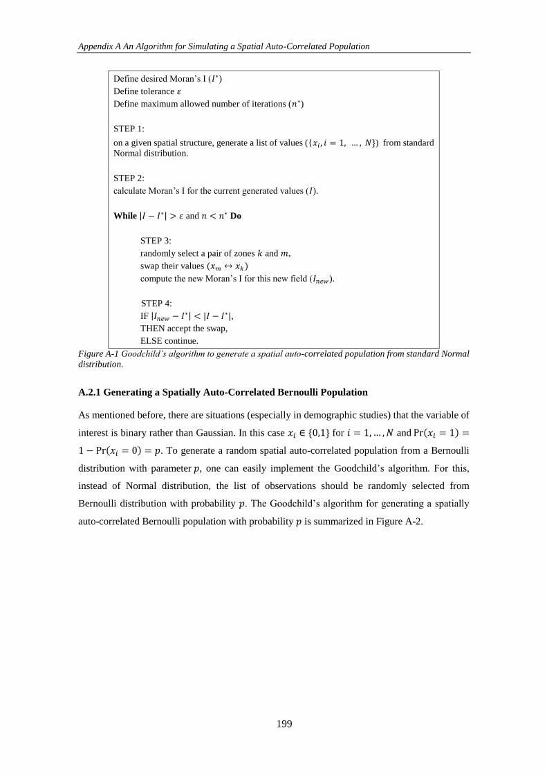
Appendix A An Algorithm for Simulating a Spatial Auto-Correlated Population
199
Define desired Moran’s I (𝐼∗)
Define tolerance 𝜀
Define maximum allowed number of iterations (𝑛∗)
STEP 1:
on a given spatial structure, generate a list of values ({𝑥𝑖 , 𝑖 = 1, … , 𝑁}) from standard
Normal distribution.
STEP 2:
calculate Moran’s I for the current generated values (𝐼).
While |𝐼 − 𝐼∗| > 𝜀 and 𝑛 < 𝑛∗ Do
STEP 3:
randomly select a pair of zones 𝑘 and 𝑚,
swap their values (𝑥𝑚 ↔ 𝑥𝑘)
compute the new Moran’s I for this new field (𝐼𝑛𝑒𝑤).
STEP 4:
IF |𝐼𝑛𝑒𝑤 − 𝐼∗| < |𝐼 − 𝐼∗|,
THEN accept the swap,
ELSE continue.
Figure A-1 Goodchild’s algorithm to generate a spatial auto-correlated population from standard Normal
distribution.
A.2.1 Generating a Spatially Auto-Correlated Bernoulli Population
As mentioned before, there are situations (especially in demographic studies) that the variable of
interest is binary rather than Gaussian. In this case 𝑥𝑖 ∈ {0,1} for 𝑖 = 1,… ,𝑁 and Pr(𝑥𝑖 = 1) =
1 − Pr(𝑥𝑖 = 0) = 𝑝. To generate a random spatial auto-correlated population from a Bernoulli
distribution with parameter 𝑝, one can easily implement the Goodchild’s algorithm. For this,
instead of Normal distribution, the list of observations should be randomly selected from
Bernoulli distribution with probability 𝑝. The Goodchild’s algorithm for generating a spatially
auto-correlated Bernoulli population with probability 𝑝 is summarized in Figure A-2.
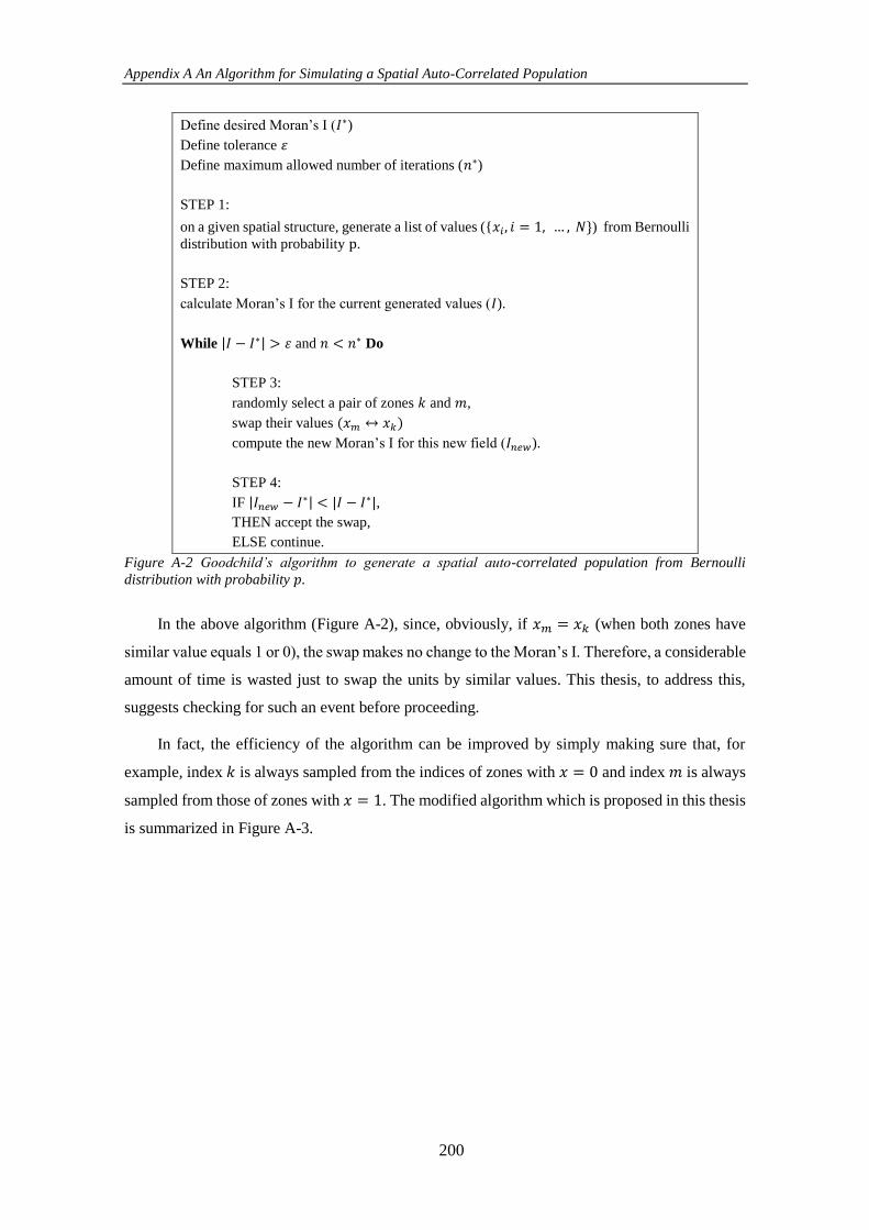
Appendix A An Algorithm for Simulating a Spatial Auto-Correlated Population
200
Define desired Moran’s I (𝐼∗)
Define tolerance 𝜀
Define maximum allowed number of iterations (𝑛∗)
STEP 1:
on a given spatial structure, generate a list of values ({𝑥𝑖 , 𝑖 = 1, … , 𝑁}) from Bernoulli
distribution with probability p.
STEP 2:
calculate Moran’s I for the current generated values (𝐼).
While |𝐼 − 𝐼∗| > 𝜀 and 𝑛 < 𝑛∗ Do
STEP 3:
randomly select a pair of zones 𝑘 and 𝑚,
swap their values (𝑥𝑚 ↔ 𝑥𝑘)
compute the new Moran’s I for this new field (𝐼𝑛𝑒𝑤).
STEP 4:
IF |𝐼𝑛𝑒𝑤 − 𝐼∗| < |𝐼 − 𝐼∗|,
THEN accept the swap,
ELSE continue.
Figure A-2 Goodchild’s algorithm to generate a spatial auto-correlated population from Bernoulli
distribution with probability 𝑝.
In the above algorithm (Figure A-2), since, obviously, if 𝑥𝑚 = 𝑥𝑘 (when both zones have
similar value equals 1 or 0), the swap makes no change to the Moran’s I. Therefore, a considerable
amount of time is wasted just to swap the units by similar values. This thesis, to address this,
suggests checking for such an event before proceeding.
In fact, the efficiency of the algorithm can be improved by simply making sure that, for
example, index 𝑘 is always sampled from the indices of zones with 𝑥 = 0 and index 𝑚 is always
sampled from those of zones with 𝑥 = 1. The modified algorithm which is proposed in this thesis
is summarized in Figure A-3.
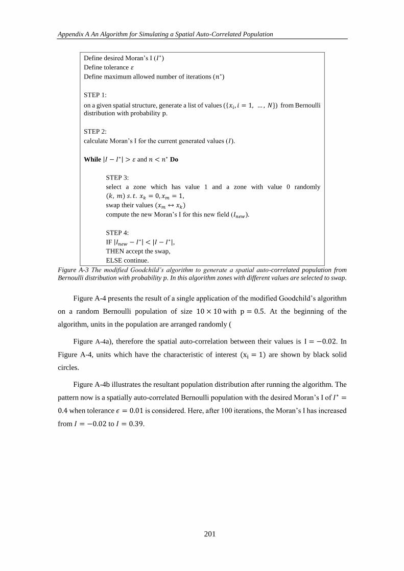
Appendix A An Algorithm for Simulating a Spatial Auto-Correlated Population
201
Define desired Moran’s I (𝐼∗)
Define tolerance 𝜀
Define maximum allowed number of iterations (𝑛∗)
STEP 1:
on a given spatial structure, generate a list of values ({𝑥𝑖 , 𝑖 = 1, … , 𝑁}) from Bernoulli
distribution with probability p.
STEP 2:
calculate Moran’s I for the current generated values (𝐼).
While |𝐼 − 𝐼∗| > 𝜀 and 𝑛 < 𝑛∗ Do
STEP 3:
select a zone which has value 1 and a zone with value 0 randomly
(𝑘, 𝑚) 𝑠. 𝑡. 𝑥𝑘 = 0, 𝑥𝑚 = 1,
swap their values (𝑥𝑚 ↔ 𝑥𝑘)
compute the new Moran’s I for this new field (𝐼𝑛𝑒𝑤).
STEP 4:
IF |𝐼𝑛𝑒𝑤 − 𝐼∗| < |𝐼 − 𝐼∗|,
THEN accept the swap,
ELSE continue.
Figure A-3 The modified Goodchild’s algorithm to generate a spatial auto-correlated population from
Bernoulli distribution with probability 𝑝. In this algorithm zones with different values are selected to swap.
Figure A-4 presents the result of a single application of the modified Goodchild’s algorithm
on a random Bernoulli population of size 10 × 10 with p = 0.5. At the beginning of the
algorithm, units in the population are arranged randomly (
Figure A-4a), therefore the spatial auto-correlation between their values is I = −0.02. In
Figure A-4, units which have the characteristic of interest (xi = 1) are shown by black solid
circles.
Figure A-4b illustrates the resultant population distribution after running the algorithm. The
pattern now is a spatially auto-correlated Bernoulli population with the desired Moran’s I of 𝐼∗ =
0.4 when tolerance 𝜖 = 0.01 is considered. Here, after 100 iterations, the Moran’s I has increased
from 𝐼 = −0.02 to 𝐼 = 0.39.
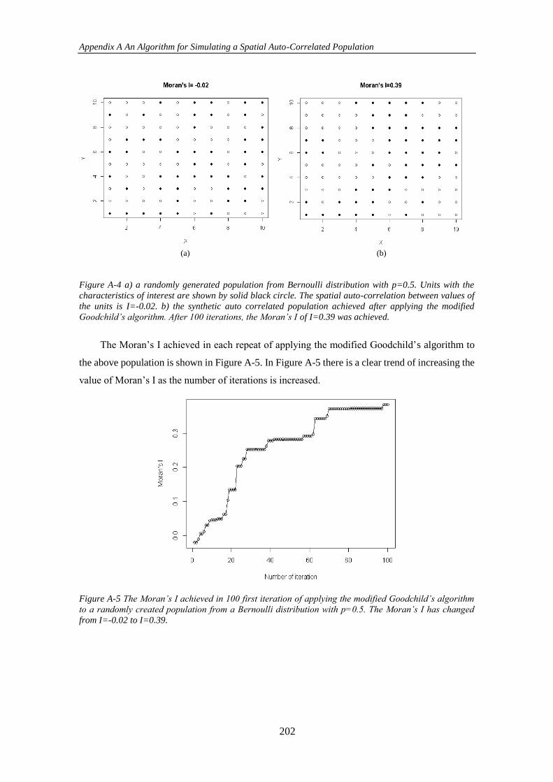
Appendix A An Algorithm for Simulating a Spatial Auto-Correlated Population
202
Figure A-4 a) a randomly generated population from Bernoulli distribution with p=0.5. Units with the
characteristics of interest are shown by solid black circle. The spatial auto-correlation between values of
the units is I=-0.02. b) the synthetic auto correlated population achieved after applying the modified
Goodchild’s algorithm. After 100 iterations, the Moran’s I of I=0.39 was achieved.
The Moran’s I achieved in each repeat of applying the modified Goodchild’s algorithm to
the above population is shown in Figure A-5. In Figure A-5 there is a clear trend of increasing the
value of Moran’s I as the number of iterations is increased.
Figure A-5 The Moran’s I achieved in 100 first iteration of applying the modified Goodchild’s algorithm
to a randomly created population from a Bernoulli distribution with p=0.5. The Moran’s I has changed
from I=-0.02 to I=0.39.
(a) (b)
Appendix A An Algorithm for Simulating a Spatial Auto-Correlated Population
203
A.3 References
Alfons, A., Kraft, S., Templ, M., & Filzmoser, P. (2010). Simulation of synthetic population data
for household surveys with application to EU-SILC. Retrieved from
Ballas, D., Clarke, G., Dorling, D., & Rossiter, D. (2007). Using SimBritain to model the
geographical impact of national government policies. Geographical Analysis, 39(1), 44-
77.
Barthelemy, J., & Toint, P. L. (2013). Synthetic population generation without a sample.
Transportation Science, 47(2), 266-279.
Efstratiadis, A., Dialynas, Y. G., Kozanis, S., & Koutsoyiannis, D. (2014). A multivariate
stochastic model for the generation of synthetic time series at multiple time scales
reproducing long-term persistence. Environmental Modelling & Software, 62, 139-152.
Goodchild, M., & Openshaw, S. (1980). Algorithm 9: Simulation of autocorrelation for aggregate
data. Environment and Planning A, 12(9), 1073-1081.
King, L. M., McLeod, A. I., & Simonovic, S. P. (2014). Simulation of historical temperatures
using a multi‐site, multivariate block resampling algorithm with perturbation.
Hydrological Processes, 28(3), 905-912.
Müller, K., Axhausen, K. W., Axhausen, K. W., & Axhausen, K. W. (2010). Population synthesis
for microsimulation: State of the art: ETH Zürich, Institut für Verkehrsplanung,
Transporttechnik, Strassen-und Eisenbahnbau (IVT).
Orton, C. R. (1982). Stochastic process and archaeological mechanism in spatial analysis. Journal
of Archaeological Science, 9(1), 1-23.
Sharif, M., & Burn, D. H. (2006). Simulating climate change scenarios using an improved K-
nearest neighbor model. Journal of hydrology, 325(1-4), 179-196.
Smith, D., Clarke, G. P., & Harland, K. (2009). Improving the synthetic data generation process
in spatial microsimulation models. Environment and Planning A, 41(5), 1251-1268.
Wilks, D. (1999). Simultaneous stochastic simulation of daily precipitation, temperature and solar
radiation at multiple sites in complex terrain. Agricultural and Forest Meteorology, 96(1-
3), 85-101.
Related Documents