The analysis of cation and anion trends from soil and ...frontiersabroad.com/wp-content/uploads/2012/09/Megan-Richardson.pdf · The analysis of cation and anion trends from soil and

The analysis of cation and anion trends from soil and water samples at the Norske Skog Tasman Pulp

and Paper Mill dump site in Kawerau, New Zealand

Megan Richardson

Abstract

The main premise of this research is to identify spatial and temporal trends of leaching cations and anions in soil and water samples. The samples are from the Norske Skog Tasman Pulp and Paper Mill waste site in Kawerau, New Zealand. In addition, the consistency of collection and experimental techniques will be explored using statistical analysis of the samples. This investigation is conducted under the hypothesis that cations and anions are leaching from mill’s waste and are contaminating both the land and river as a result. The hypothesis is based on past research performed by Cailly Howell. It was performed by monitoring ion concentrations over various transects and comparing them to ion concentrations found in adjoining water sources. This study found that ions do leach from the waste site and that even under the same procedure in-lab there can be discrepancies between specific samples. In conclusions, further studies should be performed to analyze the spatial trends using multiple sample sets.

1. Introduction Chemical leaching is one of the main

problems encountered at landfills. The movement of ions depends on a multitude of factors, including waste composition, land permeability and water table level. Many wastes are treated before they are dumped into landfills to reduce harmful chemicals and to dilute the detritus. Land permeability is a concern because the rock composition and geologic outline of an area makes it more or less prone to absorption through bed rock and faults. Water is a

main source of transportation for ions, therefore the height of the water table is important to acknowledge. If the water table is low fluid transport may be less of a concern, but if it is high transport can be imminent.

The landfill in this study is used by Norkse Skog Tasman Pulp and Paper Mill for the disposal of pulp production waste. Studies have been performed in regard to the leaching of ions from the waste into surrounding land and water features. One water feature of concern is the Tawerau

River, which is used by the local community for recreation and livelihood.

A study was performed in 2011 by Cailly Howell which showed that cations leach from soil sediments when the pH is lowered and the soil becomes more acidic (Howell, 2011). Sources of soil acidity include both rainfall and weathering (Sparks, 2003). Prompted by her work, a complementary study of the waste site was performed in 2012. Ions which leach from the sediments were compared to cations found in various water samples from sources both upstream and downstream of the waste under the hypothesis that ions are leaching from the central waste site to surrounding land and water features. This study used Atomic Absorption Spectrometry and Ion Chromatography to determine ion concentrations and results showed spatial trends throughout the site. The confirmation of ion transport is of concern because it means that the waste not only directly impacts the land on which it was situated, but also indirectly impacts the surrounding area.

In addition, the study used statistical analysis to determine the consistency of sampling practices both in the field and in the lab. Visual and calculated comparisons were employed in the investigation to find that the lab methods performed did not yield perfectly replicable results. This information promotes the use of more sample sets in order to reduce the significance of outliers.

2. Background

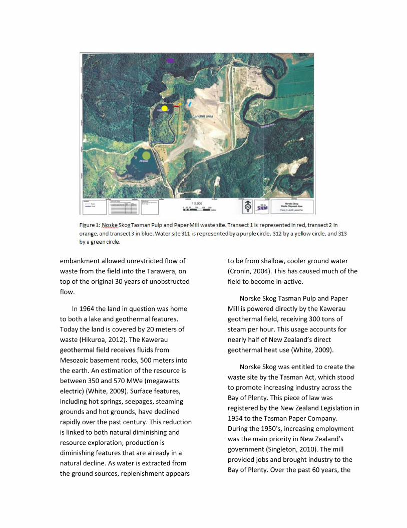
The site being tested is a waste-ground for the Norske Skog Tasman Pulp and Paper Mill, located in Kawerau, Bay of Plenty, North Island, New Zealand (Figure 1). The mill was established in 1952 and initially disposed of waste into the Tarawera River until 1964 (Hikuroa, 2012). In 1964 the Tasman Pulp and Paper Company Enabling Act was passed as a means to promote industry through the subsidence of environmental regulations (Tasman, 1954). At this time the company used the Tasman Act to force the Maori landowners of Kawerau to either sell or lease the land as a waste site. The owners chose to lease the land rather than lose it completely. This lease is set to expire in 2013, at which time Ngati Rangitihi Iwi (the owners) will regain control of the grounds. Over the past 60 years, the land and adjoining Tarawera River have been contaminated and polluted under the blanket of social and economic benefits (Environment, 2009).

The land which waste was and is still being disposed on is permeable, faulted and geothermally active (Hikuroa, 2012). The water table in the area is high, and the site is between an artificial pond and the Tarawera River. The river is separated by an embankment, built in the 1980s. It has failed three times in its lifespan (Hikuroa, 2012). All of these attributes are clear indicators as to why it is possible for contaminants to spread from the paper waste. Permeable and faulted grounds offer pathways for transport over a wide area. Elevated water tables indicate that the ground water is shallow, meaning that if water is contaminated, it has the ability to continue flowing along the table. In addition, the three failures of the

embankment allowed unrestricted flow of waste from the field into the Tarawera, on top of the original 30 years of unobstructed flow.

In 1964 the land in question was home to both a lake and geothermal features. Today the land is covered by 20 meters of waste (Hikuroa, 2012). The Kawerau geothermal field receives fluids from Mesozoic basement rocks, 500 meters into the earth. An estimation of the resource is between 350 and 570 MWe (megawatts electric) (White, 2009). Surface features, including hot springs, seepages, steaming grounds and hot grounds, have declined rapidly over the past century. This reduction is linked to both natural diminishing and resource exploration; production is diminishing features that are already in a natural decline. As water is extracted from the ground sources, replenishment appears

to be from shallow, cooler ground water (Cronin, 2004). This has caused much of the field to become in-active.

Norske Skog Tasman Pulp and Paper Mill is powered directly by the Kawerau geothermal field, receiving 300 tons of steam per hour. This usage accounts for nearly half of New Zealand’s direct geothermal heat use (White, 2009).

Norske Skog was entitled to create the waste site by the Tasman Act, which stood to promote increasing industry across the Bay of Plenty. This piece of law was registered by the New Zealand Legislation in 1954 to the Tasman Paper Company. During the 1950’s, increasing employment was the main priority in New Zealand’s government (Singleton, 2010). The mill provided jobs and brought industry to the Bay of Plenty. Over the past 60 years, the

mill has become the Norske Skog Tasman Pulp and Paper Mill, and is still providing jobs and industry in the bay area. Today the mill contributes over $1 billion annually to the New Zealand economy. It is the largest single employer in the eastern Bay of Plenty (Hikuroa, 2012).

With the 60-year lease’s expiration fast approaching, the Ngati Rangitihi Iwi has been planning a course of action. For matters concerning the land, the Iwi is represented by a group of trustees. The Trustees are currently working on a remediation plan. Their intention is an attempt to return the land to its natural Mauri condition upon lease expiration (Hikuroa, 2012). The plan will combine science with indigenous knowledge, using the Mauri Model. The Maori Model is a decision-making framework that provides a culturally based template within which indigenous values are explicitly empowered alongside knowledge (Morgan, 2006). Our work, in analyzing soil and water samples, will be directly used to assess the impact on Mauri. The information on cations present across the plot will be compared to a retrospective of the time before the land was contaminated. The goal of remediation is to return the Mauri to the land, meaning to return the land to its condition before it was leased to Norske Skog. The contaminants therefore will be compared to initial concentrations rather than national environmental standards (Hikuroa, 2003).

Water sources in the vicinity of the waste site include the Tarawera River, Urupa Pond, A8 Pond, connecting canal (between the ponds), and Te Wai U o

Tuwharetoa. The last of which is upstream from the waste site, and the others are located around the site. These bodies facilitate water and sediment movement both as surface features and ground water.

3. Materials and Methods 3.1. Sediment

A total of 42 sediment samples, along three separate transects, were taken from Norske Skog Tasman Pulp and Paper Mill’s waste site in Kawerau, New Zealand. The samples were collected on February 2, 2012 from 12:15 until 12:50. Between 50 and 200 grams of sediment were taken from each site and placed into a plastic bag, which was then labeled, sealed, and transported to Auckland University for processing. To attain a more accurate representation of soil content, two samples were taken from each sample site, labeled A and B.

The first transect, labeled T1, consists of 12 sample sites and 24 samples. Each site is 2 meters apart along the transect line, originating 1 meter from Urupa Pond and extending a total of 23 meters from the pond, towards the landfill area. This transect was selected to show a spatial pattern starting from the water source and extending towards the actual waste bed. The second transect, labeled T2, consists of 3 sample sites and 6 samples. The first sample was located 2 meters to the west of the road, the second in the center of the road, and the third 2 meters to the east of the road. This transect was selected to monitor how well the road acted as a barrier between the waste and Urupa pond. The third transect, T3, consists of 6 sample

sites and 12 samples. Similar to transect 1, each sample is spaced 2 meters apart along the transect line. T3 originates 50 meters north of T2, further down the road, and extends 13 meters onto the landfill area. The last transect was used to determine how much of the waste leached from the middle of the waste bed extending away towards the road.

3.2. Water

Three water samples were taken from three sample sites. The samples were collected on February 2, 2012, between 11:00 and 12:00. The first sample site, labeled AZ311, is called “Te Wai U o Tuwharetoa,” which means “the life giving water of Tuwharetoa” (Council). This existing warm-water spring is located upstream from the pulp and paper dumping site, and can act as a control. The second site, AZ312, is Urupa pond, which is where transect 1 of the sediment samples began. Urupa pond is separated from the landfill by a road. The third site, AZ313, is the A8 pond, which is in very close proximity to a tail of the landfill.

Each sample was extracted by placing the plastic collection bottle directly in the water source, rinsing three times, and then filling completely. Then the sample was filtered, using .45 micrometer filters, and separated into labeled cation and anion bottles. These bottles were then bagged, according to site, and placed into a cooler for transport to Auckland University.

3.3. Experimental set-up

All laboratory experiments took place in University of Auckland HSB water quality

laboratory. The samples were initially organized by transect and sample site, with the water samples separated from the soil samples. To prepare the sediment for analysis, 4 grams of each sample was measured and added to 40 mL of deionized water in a centrifuge tube, which was labeled with transect, site, and group (example: T1S1Amix). The tube was then shaken vigorously for 5 minutes and then placed on a sample stand to sit and separate for 4 hours. This procedure was repeated with all 42 sediment samples.

After the allotted 4 hours, each sample was decanted into a beaker. Using a syringe and a .45 micrometer filter, approximately 20 mL of the extracted liquid was then filtered and placed in a new labeled centrifuge tube (example: T1S1A). After all samples were processed in such manner, there were 42 liquid samples prepared for cation spectrometry and anion chromatography.

The water samples had previously been filtered in the field, immediately after collection. In the lab, 20 mL of each was measured in a graduated cylinder and poured into a labeled centrifuge tube, specified as either a cation or anion sample and separated into groups A and B (example: AZ311A-cation).

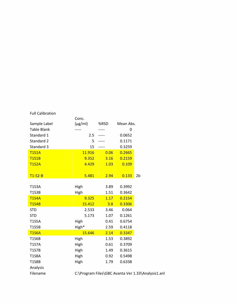
3.4. Cation concentrations Cation concentrations were measured

Atomic Absorption Spectrometry. The cations in question were sodium, potassium, magnesium and calcium, and the concentrations were recorded in parts per million (ppm). The in-lab analysis occurred from May 7 through 22, 2012. During the experiment, the bulb in the

spectrometry machine that pertained to the analysis of potassium burned out and a replacement was not available. Therefore, potassium was removed from the observed cations.

For each cation, three standards were used with pre-determined concentrations. The standards were utilized to calibrate the machine and monitor irregularities. Once the machine was calibrated for the specific cation, the three transects and water samples were tested. The extraction tube of the machine was placed directly in each centrifuge tube and after the sample had been analyzed by the machine, the computer recorded a specific cation concentration. This process was repeated with all 48 samples for a specific cation, and then the next two cations were analyzed using the same procedure.

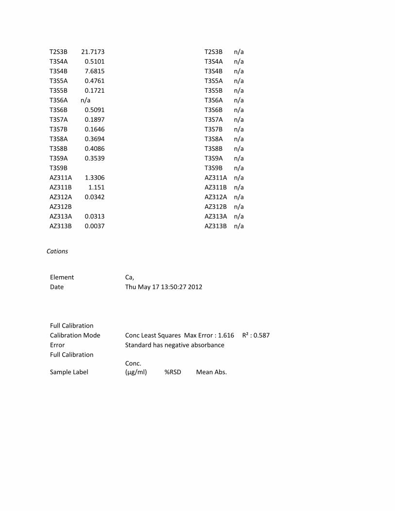
3.5. Anion concentrations

Anion concentrations were measured using Ion Chromatography. The anions in question were chloride, sulphate, nitrate and phosphate, and the concentrations were recorded in parts per million (ppm). The in-lab analysis of anions occurred from May 7 through 22, 2012, as did the cations.

The samples were prepared for chromatography by extracting the liquid with a pipette and placing about 5 mL of each sample in a small, plastic tube. Five tubes fit together in a frame that would eventually be placed directly into the machine for analysis. Each tube was fitted with a rubber stopper that sealed the

samples completely. The samples were ordered by transect, with both sample A and B next to one another, followed by the water samples.

The chromatography ran overnight and analyzed each sample for anion concentrations. All recordable levels of anions were graphed on the computer. Each peak was manually identified and labeled as a specific anion, and the concentration was provided by the computer program.

3.6. Data interpretation

After all of the raw data was collected, it was imported into excel for configuration. The two sets of data for each transect were separated in order to view each individually.

4. Results and Discussion 4.1. Cation leaching trends

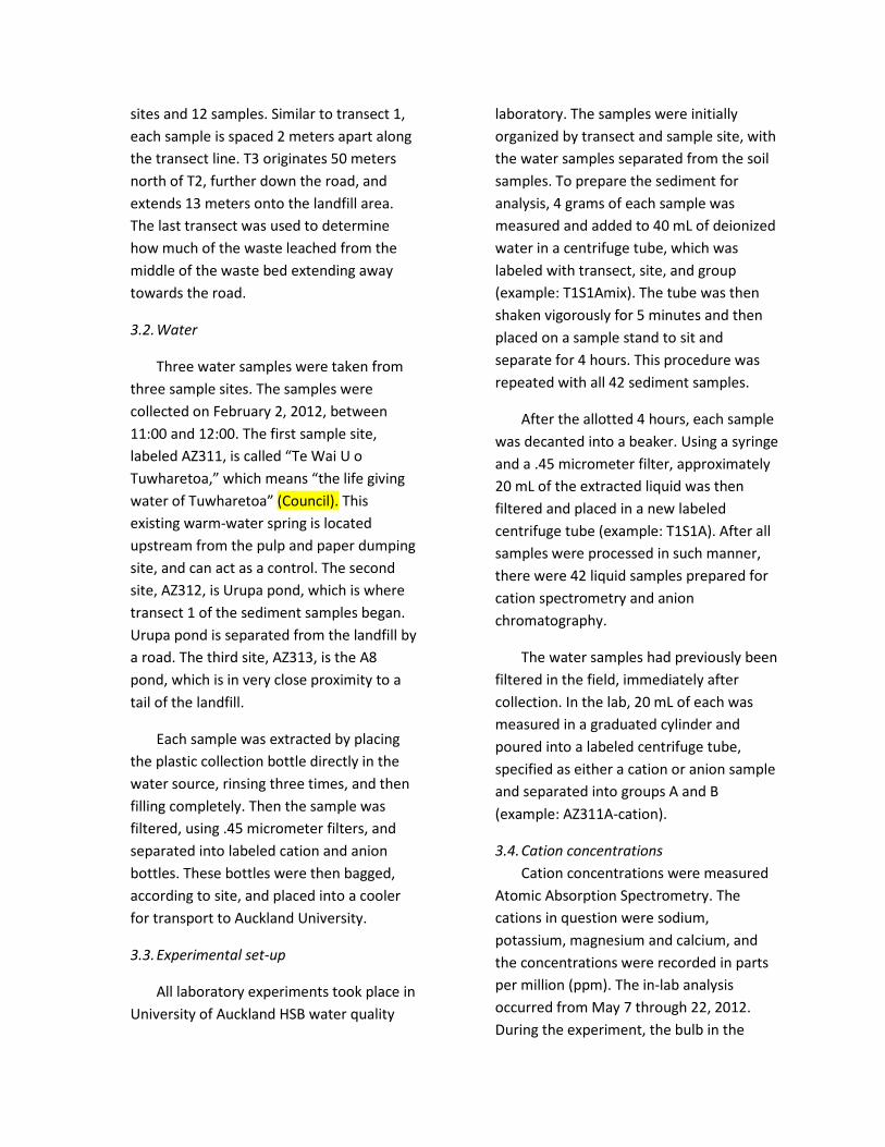
Upon review of data collected through absorption spectrometry, trends were observed pertaining to the spatial distribution of cations in the sediment samples. Transects 1 and 3 were plotted as concentration (parts per million) verses distance down the transect line (meters), and then a linear trend line was added show the overall tendency of cation movement.

In transect 1, which ran from Urupa pond inland towards the landfill area, there was a clear increase in calcium-ion concentrations (figure 1), which averages

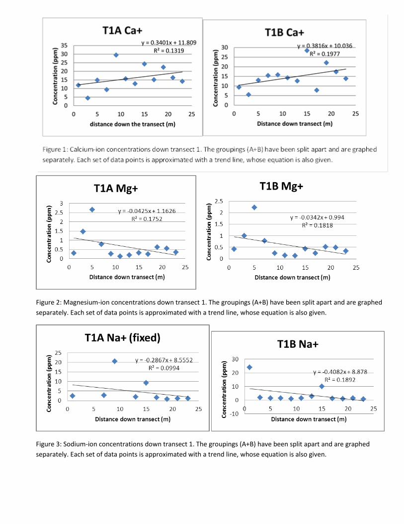
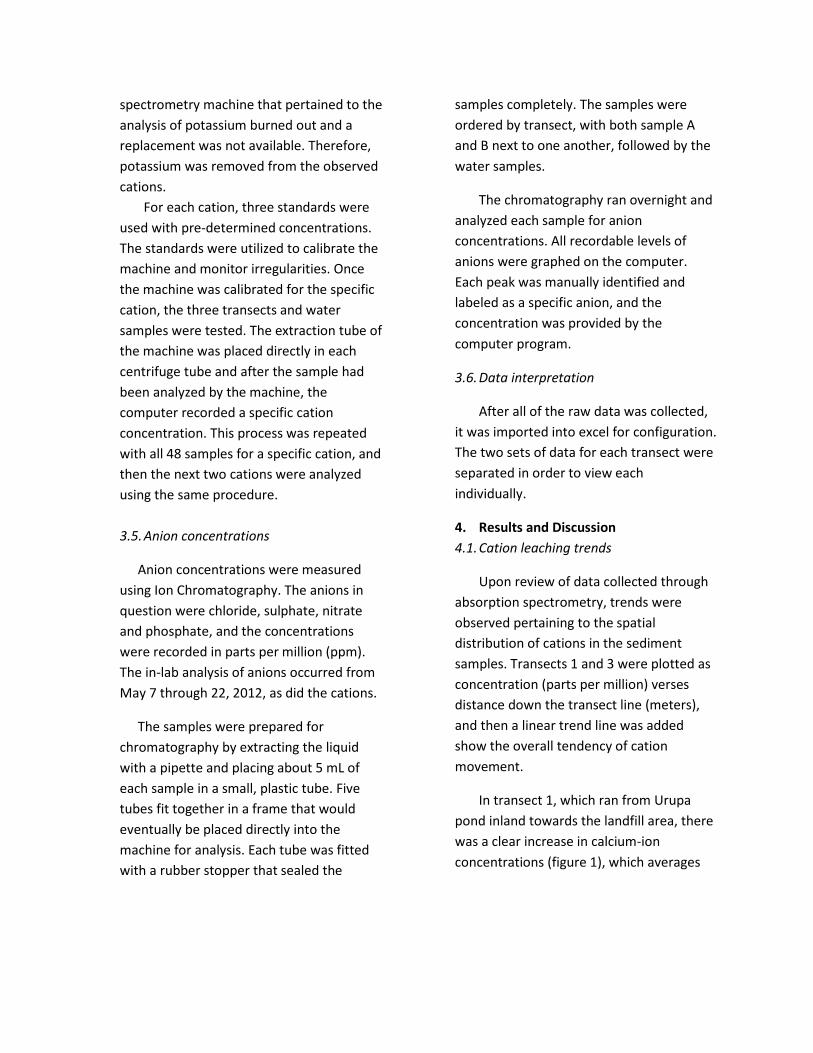
Figure 2: Magnesium-ion concentrations down transect 1. The groupings (A+B) have been split apart and are graphed separately. Each set of data points is approximated with a trend line, whose equation is also given.

Figure 3: Sodium-ion concentrations down transect 1. The groupings (A+B) have been split apart and are graphed separately. Each set of data points is approximated with a trend line, whose equation is also given.

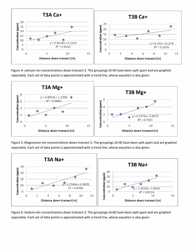
Figure 4: calcium-ion concentrations down transect 3. The groupings (A+B) have been split apart and are graphed separately. Each set of data points is approximated with a trend line, whose equation is also given.

Figure 5: Magnesium-ion concentrations down transect 3. The groupings (A+B) have been split apart and are graphed separately. Each set of data points is approximated with a trend line, whose equation is also given.

Figure 6: Sodium-ion concentrations down transect 3. The groupings (A+B) have been split apart and are graphed separately. Each set of data points is approximated with a trend line, whose equation is also given.

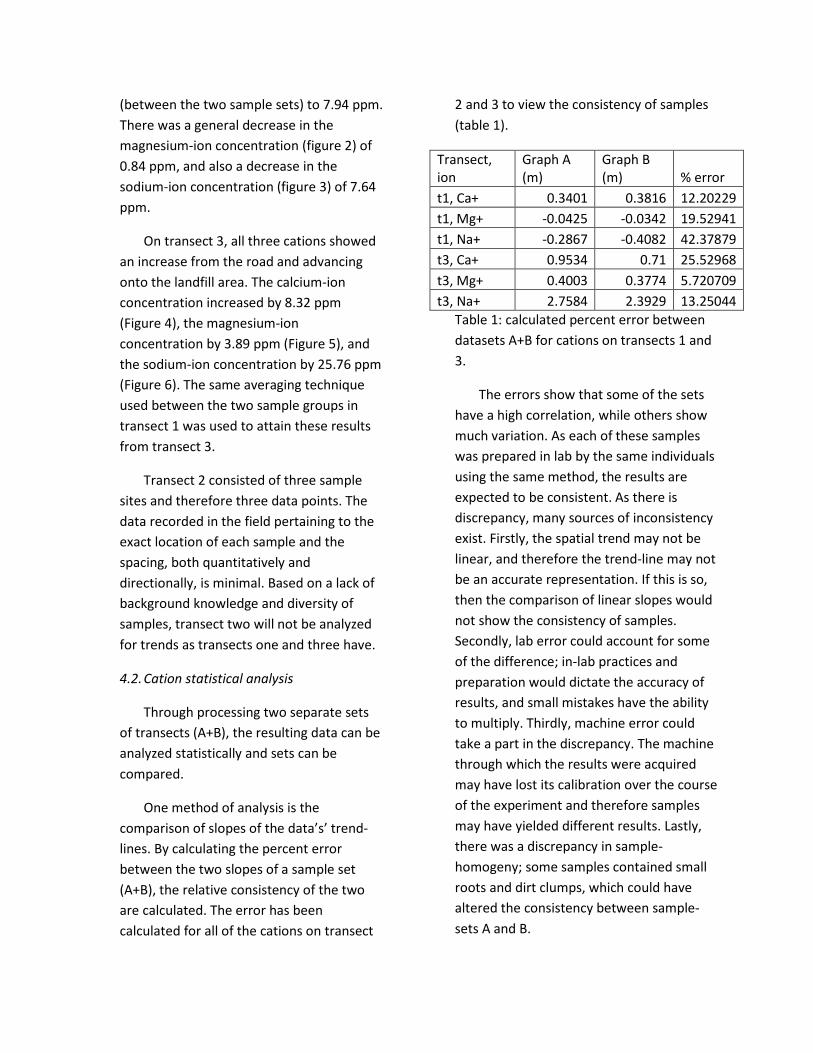
(between the two sample sets) to 7.94 ppm. There was a general decrease in the magnesium-ion concentration (figure 2) of 0.84 ppm, and also a decrease in the sodium-ion concentration (figure 3) of 7.64 ppm.

On transect 3, all three cations showed an increase from the road and advancing onto the landfill area. The calcium-ion concentration increased by 8.32 ppm (Figure 4), the magnesium-ion concentration by 3.89 ppm (Figure 5), and the sodium-ion concentration by 25.76 ppm (Figure 6). The same averaging technique used between the two sample groups in transect 1 was used to attain these results from transect 3.

Transect 2 consisted of three sample sites and therefore three data points. The data recorded in the field pertaining to the exact location of each sample and the spacing, both quantitatively and directionally, is minimal. Based on a lack of background knowledge and diversity of samples, transect two will not be analyzed for trends as transects one and three have.

4.2. Cation statistical analysis

Through processing two separate sets of transects (A+B), the resulting data can be analyzed statistically and sets can be compared.

One method of analysis is the comparison of slopes of the data’s’ trend-lines. By calculating the percent error between the two slopes of a sample set (A+B), the relative consistency of the two are calculated. The error has been calculated for all of the cations on transect

2 and 3 to view the consistency of samples (table 1).

Transect, ion

Graph A (m)

Graph B (m) % error

t1, Ca+ 0.3401 0.3816 12.20229 t1, Mg+ -0.0425 -0.0342 19.52941 t1, Na+ -0.2867 -0.4082 42.37879 t3, Ca+ 0.9534 0.71 25.52968 t3, Mg+ 0.4003 0.3774 5.720709 t3, Na+ 2.7584 2.3929 13.25044

Table 1: calculated percent error between datasets A+B for cations on transects 1 and 3.

The errors show that some of the sets have a high correlation, while others show much variation. As each of these samples was prepared in lab by the same individuals using the same method, the results are expected to be consistent. As there is discrepancy, many sources of inconsistency exist. Firstly, the spatial trend may not be linear, and therefore the trend-line may not be an accurate representation. If this is so, then the comparison of linear slopes would not show the consistency of samples. Secondly, lab error could account for some of the difference; in-lab practices and preparation would dictate the accuracy of results, and small mistakes have the ability to multiply. Thirdly, machine error could take a part in the discrepancy. The machine through which the results were acquired may have lost its calibration over the course of the experiment and therefore samples may have yielded different results. Lastly, there was a discrepancy in sample-homogeny; some samples contained small roots and dirt clumps, which could have altered the consistency between sample-sets A and B.

4.3. Anion leaching trends

As with the cations in the experiment, anion concentrations (ppm) were plotted against the distance down the transect

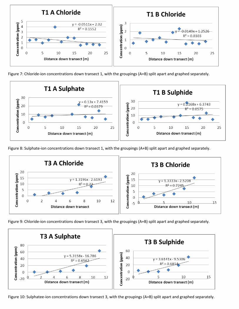
Figure 7: Chloride-ion concentrations down transect 1, with the groupings (A+B) split apart and graphed separately.

Figure 8: Sulphate-ion concentrations down transect 1, with the groupings (A+B) split apart and graphed separately.

Figure 9: Chloride-ion concentrations down transect 3, with the groupings (A+B) split apart and graphed separately.

Figure 10: Sulphatee-ion concentrations down transect 3, with the groupings (A+B) split apart and graphed separately.

4.3. Anion leaching trends

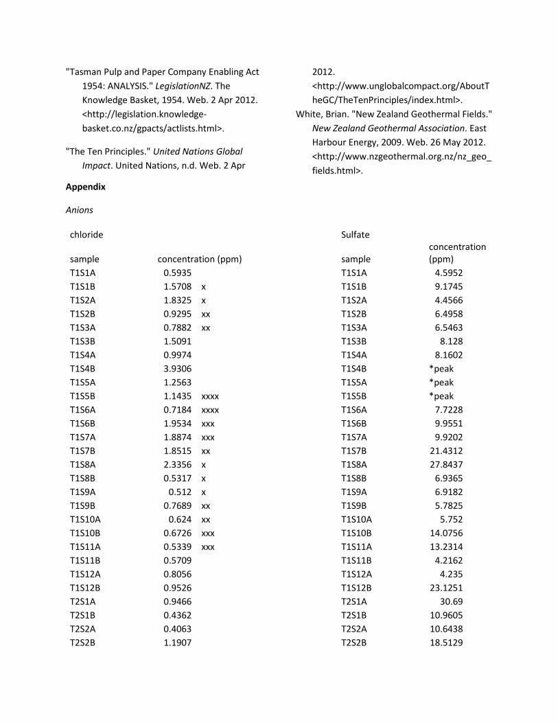
As with the cations in the experiment, anion concentrations (ppm) were plotted against the distance down the transect (meters) and a linear trend line was added. The anions that were tested included chloride, sulphate, nitrate and phosphate. Of the data inquired about, nitrate and phosphate yielded inconsistent results; many concentrations were missing from the data sheets. Only chloride and sulphate yielded significant data which could be graphed and tabulated for trends. Therefore, only chloride and sulphate were used in the analysis of anion leaching trends.

On transect 1, there was a general decrease in chloride concentration (Figure 7) which averaged to 0.73 ppm. Sulphate showed a minimal increase down the transect of 3.81 ppm (Figure 8).

On transect 3, both chloride and Sulphate showed a more significant increasing trend. Chloride increased by 13.26 ppm (Figure 9) and Sulphate by 44.65 ppm (Figure 10). On both transect 1 and 3 the change in concentration was an average between the two datasets.

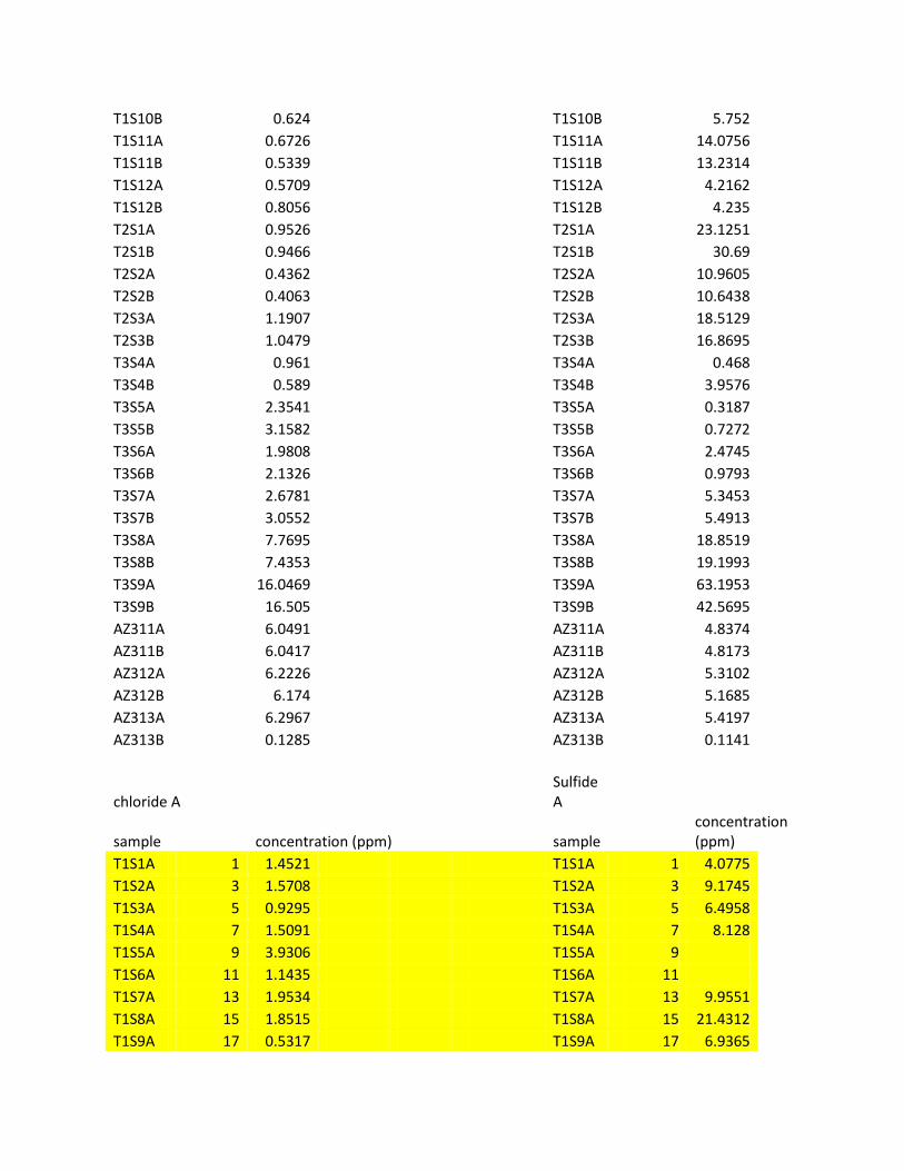
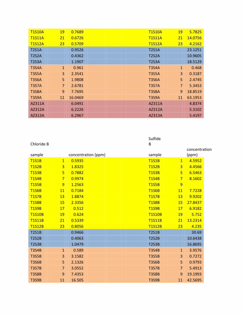
4.4. Anion statistical analysis

To show the value of multiple statistical analyses, a different method will be used to compare anion datasets A+B from the cation analysis. Instead of a slope comparison, a visual alignment will be used to check for relative data consistency.

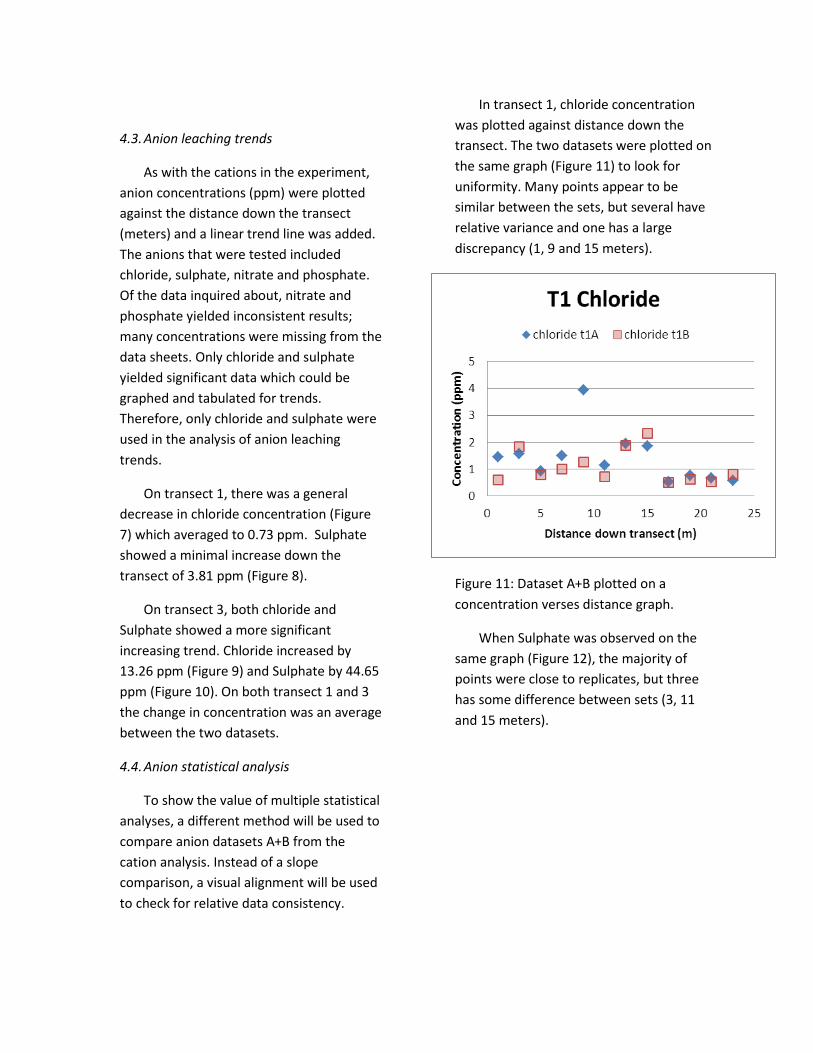
In transect 1, chloride concentration was plotted against distance down the transect. The two datasets were plotted on the same graph (Figure 11) to look for uniformity. Many points appear to be similar between the sets, but several have relative variance and one has a large discrepancy (1, 9 and 15 meters).

Figure 11: Dataset A+B plotted on a concentration verses distance graph.

When Sulphate was observed on the same graph (Figure 12), the majority of points were close to replicates, but three has some difference between sets (3, 11 and 15 meters).

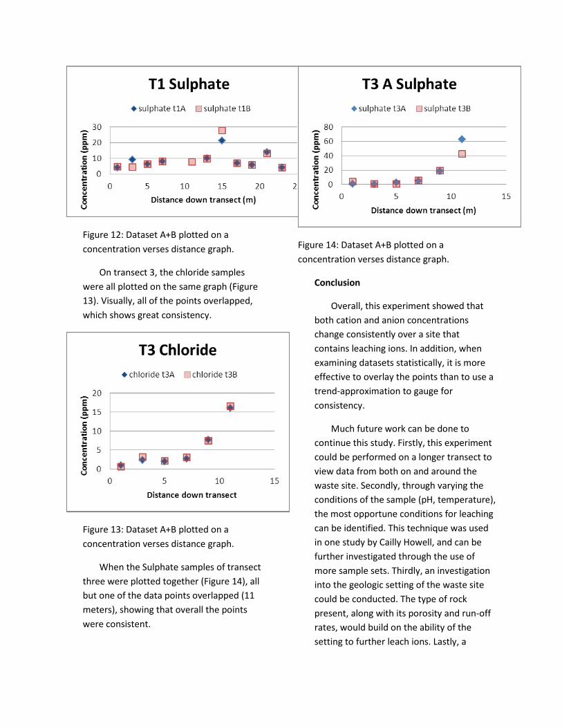
Figure 12: Dataset A+B plotted on a concentration verses distance graph.

On transect 3, the chloride samples were all plotted on the same graph (Figure 13). Visually, all of the points overlapped, which shows great consistency.

Figure 13: Dataset A+B plotted on a concentration verses distance graph.

When the Sulphate samples of transect three were plotted together (Figure 14), all but one of the data points overlapped (11 meters), showing that overall the points were consistent.

Figure 14: Dataset A+B plotted on a concentration verses distance graph.

Conclusion

Overall, this experiment showed that both cation and anion concentrations change consistently over a site that contains leaching ions. In addition, when examining datasets statistically, it is more effective to overlay the points than to use a trend-approximation to gauge for consistency.

Much future work can be done to continue this study. Firstly, this experiment could be performed on a longer transect to view data from both on and around the waste site. Secondly, through varying the conditions of the sample (pH, temperature), the most opportune conditions for leaching can be identified. This technique was used in one study by Cailly Howell, and can be further investigated through the use of more sample sets. Thirdly, an investigation into the geologic setting of the waste site could be conducted. The type of rock present, along with its porosity and run-off rates, would build on the ability of the setting to further leach ions. Lastly, a

chemical analysis of the Norske Skog Tasman waste could be conducted to determine what exactly is being put into the land to possibly leach into surrounding grounds.

Acknowledgements

Thank you to Russel Clarke, who taught us how to use all of the lab equipment and was flexible in allowing us to perform our experiment. To Angela who guided us in our reports and steered us down the correct path. And to Dan and Jan who have worked with us all semester towards our final report!

References

Bruere, Andy. "Pulp and Paper Mills in the Bay of Plenty." . Environment Bay of Plenty Regional Counsel, April 2003. Web. 2 Apr 2012. <http://monitoring.boprc.govt.nz/Reports/Report-0304-PulpAndPaperMillsInTheBOP.pdf>.

Cronin, John. "Geothermal Resources." Tarawera River Catchment Plan. Bay of Plenty Regional Council, 1 February 2004. Web. 26 May 2012. <http://monitoring.boprc.govt.nz/Plans/Plan-040201-RegionalPlanForTheTaraweraRiverCatchmentChapter_17.pdf>.

Davison, Isaac. "Mill gets 25-year pollution consent." New Zealand Herald 16 11 2009, n. pag. Web. 2 Apr. 2012. <http://www.nzherald.co.nz/nz/news/article.cfm?c_id=1&objectid=10603488>.

"Environment permit decision upsets mill’s detractors." i-grafix. 17 oct 2009: n. page. Web. 2 Apr. 2012.

<http://www.i-grafix.com/index.php/news/new-zealand/environment-permit-decision-upsets-mills-detractors.html>.

Hikuroa, Daniel, Angela Slade, and Darren Gravley. "Implementing Māori indigenous knowledge." MAI Journal. (2003): n. page. Print.

Howell, Cailly. Determining the concentration of calcium, potassium, magnesium, and zinc cations leached from solid waste generated by the Norske Skog Tasman Pulp and Paper Mill under varying pH conditions. University of Auckland, 2011. Print.

Morgan, T. K. K. B. (2006). Decision-support tools and the indigenous paradigm. Engineering Sustainability, 159(ES4), 169–177.

New Zealand. Parlimentary Counsel Office.

Tasman Pulp and Paper Company Enabling Act . 1954. Print. <http://www.nzlii.org/nz/legis/hist_act/tpapcea19541954n82374/>.

Norske Skog. Annual Report: Norwegian Paper Tradition. Norske Skog, 2010.

Hikuroa, Daniel. "Norske Skog Pulp and Paper Mill." New Zealand Earth Systems Course Book. Frontiers Abroad, 2012. 123-125. Print.

Singleton, John. "An Economic History of New Zealand in the Nineteenth and Twentieth Centuries." EH.Net. 2 May 2010. Economic History Association, Web. 3 Apr 2012. <http://eh.net/encyclopedia/article/Singleton.NZ>.

Sparks, Donald; Environmental Soil Chemistry. 2003, Academic Press, London, UK

"Tasman Pulp and Paper Company Enabling Act 1954: ANALYSIS." LegislationNZ. The Knowledge Basket, 1954. Web. 2 Apr 2012. <http://legislation.knowledge-basket.co.nz/gpacts/actlists.html>.

"The Ten Principles." United Nations Global Impact. United Nations, n.d. Web. 2 Apr

2012. <http://www.unglobalcompact.org/AboutTheGC/TheTenPrinciples/index.html>.

White, Brian. "New Zealand Geothermal Fields." New Zealand Geothermal Association. East Harbour Energy, 2009. Web. 26 May 2012. <http://www.nzgeothermal.org.nz/nz_geo_fields.html>.

Appendix

Anions

chloride

Sulfate

sample

concentration (ppm)

sample

concentration (ppm)

T1S1A

0.5935

T1S1A

4.5952 T1S1B

1.5708 x

T1S1B

9.1745

T1S2A

1.8325 x

T1S2A

4.4566 T1S2B

0.9295 xx

T1S2B

6.4958

T1S3A

0.7882 xx

T1S3A

6.5463 T1S3B

1.5091

T1S3B

8.128

T1S4A

0.9974

T1S4A

8.1602 T1S4B

3.9306

T1S4B

*peak

T1S5A

1.2563

T1S5A

*peak T1S5B

1.1435 xxxx

T1S5B

*peak

T1S6A

0.7184 xxxx

T1S6A

7.7228 T1S6B

1.9534 xxx

T1S6B

9.9551

T1S7A

1.8874 xxx

T1S7A

9.9202 T1S7B

1.8515 xx

T1S7B

21.4312

T1S8A

2.3356 x

T1S8A

27.8437 T1S8B

0.5317 x

T1S8B

6.9365

T1S9A

0.512 x

T1S9A

6.9182 T1S9B

0.7689 xx

T1S9B

5.7825

T1S10A

0.624 xx

T1S10A

5.752 T1S10B

0.6726 xxx

T1S10B

14.0756

T1S11A

0.5339 xxx

T1S11A

13.2314 T1S11B

0.5709

T1S11B

4.2162

T1S12A

0.8056

T1S12A

4.235 T1S12B

0.9526

T1S12B

23.1251

T2S1A

0.9466

T2S1A

30.69 T2S1B

0.4362

T2S1B

10.9605

T2S2A

0.4063

T2S2A

10.6438 T2S2B

1.1907

T2S2B

18.5129

T2S3A

1.0479

T2S3A

16.8695 T2S3B

0.961

T2S3B

0.468

T3S4A

0.589

T3S4A

3.9576 T3S4B

2.3541

T3S4B

0.3187

T3S5A

3.1582

T3S5A

0.7272 T3S5B

1.9808

T3S5B

2.4745

T3S6A

2.1326

T3S6A

0.9793 T3S6B

2.6781

T3S6B

5.3453

T3S7A

3.0552

T3S7A

5.4913 T3S7B

7.7695

T3S7B

18.8519

T3S8A

7.4353

T3S8A

19.1993 T3S8B

16.0469

T3S8B

63.1953

T3S9A

16.505

T3S9A

42.5695 T3S9B

T3S9B

AZ311A

6.0491

AZ311A

4.8374 AZ311B

6.0417

AZ311B

4.8173

AZ312A

6.2226

AZ312A

5.3102 AZ312B

6.174

AZ312B

5.1685

AZ313A

6.2967

AZ313A

5.4197 AZ313B

0.1285

AZ313B

0.1141

chloride

Sulfate

sample

concentration (ppm)

sample

concentration (ppm)

T1S1A

1.4521

T1S1A

4.0775 T1S1B

0.5935

T1S1B

4.5952

T1S2A

1.5708

T1S2A

9.1745 T1S2B

1.8325

T1S2B

4.4566

T1S3A

0.9295

T1S3A

6.4958 T1S3B

0.7882

T1S3B

6.5463

T1S4A

1.5091

T1S4A

8.128 T1S4B

0.9974

T1S4B

8.1602

T1S5A

3.9306

T1S5A

*peak T1S5B

1.2563

T1S5B

*peak

T1S6A

1.1435

T1S6A

*peak T1S6B

0.7184

T1S6B

7.7228

T1S7A

1.9534

T1S7A

9.9551 T1S7B

1.8874

T1S7B

9.9202

T1S8A

1.8515

T1S8A

21.4312 T1S8B

2.3356

T1S8B

27.8437

T1S9A

0.5317

T1S9A

6.9365 T1S9B

0.512

T1S9B

6.9182

T1S10A

0.7689

T1S10A

5.7825

T1S10B

0.624

T1S10B

5.752 T1S11A

0.6726

T1S11A

14.0756

T1S11B

0.5339

T1S11B

13.2314 T1S12A

0.5709

T1S12A

4.2162

T1S12B

0.8056

T1S12B

4.235 T2S1A

0.9526

T2S1A

23.1251

T2S1B

0.9466

T2S1B

30.69 T2S2A

0.4362

T2S2A

10.9605

T2S2B

0.4063

T2S2B

10.6438 T2S3A

1.1907

T2S3A

18.5129

T2S3B

1.0479

T2S3B

16.8695 T3S4A

0.961

T3S4A

0.468

T3S4B

0.589

T3S4B

3.9576 T3S5A

2.3541

T3S5A

0.3187

T3S5B

3.1582

T3S5B

0.7272 T3S6A

1.9808

T3S6A

2.4745

T3S6B

2.1326

T3S6B

0.9793 T3S7A

2.6781

T3S7A

5.3453

T3S7B

3.0552

T3S7B

5.4913 T3S8A

7.7695

T3S8A

18.8519

T3S8B

7.4353

T3S8B

19.1993 T3S9A

16.0469

T3S9A

63.1953

T3S9B

16.505

T3S9B

42.5695 AZ311A

6.0491

AZ311A

4.8374

AZ311B

6.0417

AZ311B

4.8173 AZ312A

6.2226

AZ312A

5.3102

AZ312B

6.174

AZ312B

5.1685 AZ313A

6.2967

AZ313A

5.4197

AZ313B

0.1285

AZ313B

0.1141

chloride A

Sulfide A

sample

concentration (ppm)

sample

concentration (ppm)

T1S1A 1 1.4521 T1S1A 1 4.0775 T1S2A 3 1.5708 T1S2A 3 9.1745 T1S3A 5 0.9295 T1S3A 5 6.4958 T1S4A 7 1.5091 T1S4A 7 8.128 T1S5A 9 3.9306 T1S5A 9 T1S6A 11 1.1435 T1S6A 11 T1S7A 13 1.9534 T1S7A 13 9.9551 T1S8A 15 1.8515 T1S8A 15 21.4312 T1S9A 17 0.5317 T1S9A 17 6.9365

T1S10A 19 0.7689 T1S10A 19 5.7825 T1S11A 21 0.6726 T1S11A 21 14.0756 T1S12A 23 0.5709 T1S12A 23 4.2162 T2S1A 0.9526 T2S1A 23.1251 T2S2A 0.4362 T2S2A 10.9605 T2S3A 1.1907 T2S3A 18.5129 T3S4A 1 0.961 T3S4A 1 0.468 T3S5A 3 2.3541 T3S5A 3 0.3187 T3S6A 5 1.9808 T3S6A 5 2.4745 T3S7A 7 2.6781 T3S7A 7 5.3453 T3S8A 9 7.7695 T3S8A 9 18.8519 T3S9A 11 16.0469 T3S9A 11 63.1953 AZ311A 6.0491 AZ311A 4.8374 AZ312A 6.2226 AZ312A 5.3102 AZ313A 6.2967 AZ313A 5.4197

Chloride B

Sulfide B

sample

concentration (ppm)

sample

concentration (ppm)

T1S1B 1 0.5935 T1S1B 1 4.5952 T1S2B 3 1.8325 T1S2B 3 4.4566 T1S3B 5 0.7882 T1S3B 5 6.5463 T1S4B 7 0.9974 T1S4B 7 8.1602 T1S5B 9 1.2563 T1S5B 9 T1S6B 11 0.7184 T1S6B 11 7.7228 T1S7B 13 1.8874 T1S7B 13 9.9202 T1S8B 15 2.3356 T1S8B 15 27.8437 T1S9B 17 0.512 T1S9B 17 6.9182 T1S10B 19 0.624 T1S10B 19 5.752 T1S11B 21 0.5339 T1S11B 21 13.2314 T1S12B 23 0.8056 T1S12B 23 4.235 T2S1B 0.9466 T2S1B 30.69 T2S2B 0.4063 T2S2B 10.6438 T2S3B 1.0479 T2S3B 16.8695 T3S4B 1 0.589 T3S4B 1 3.9576 T3S5B 3 3.1582 T3S5B 3 0.7272 T3S6B 5 2.1326 T3S6B 5 0.9793 T3S7B 7 3.0552 T3S7B 7 5.4913 T3S8B 9 7.4353 T3S8B 9 19.1993 T3S9B 11 16.505 T3S9B 11 42.5695

AZ311B 6.0417 AZ311B 4.8173 AZ312B 6.174 AZ312B 5.1685 AZ313B 0.1285 AZ313B 0.1141 Nitrate

Phosphate

sample concentration (ppm)

sample

concentration (ppm)

T1S1A 24.2113

T1S1A 64.964 T1S1B n/a

T1S1B n/a

T1S2A 11.907

T1S2A 11.8811 T1S2B 78.1385

T1S2B n/a

T1S3A 60.796

T1S3A n/a T1S3B 37.6012

T1S3B 53.9347

T1S4A 37.9403

T1S4A n/a T1S4B n/a

T1S4B n/a

T1S5A 25.9135

T1S5A *peak T1S5B 15.0333

T1S5B *peak

T1S6A 15.0934

T1S6A n/a T1S6B 10.9682

T1S6B 15.4417

T1S7A 9.5109

T1S7A *peak T1S7B 1.7078

T1S7B n/a

T1S8A 5.5153

T1S8A n/a T1S8B 0.414

T1S8B n/a

T1S9A 0.3702

T1S9A 32.2089 T1S9B n/a

T1S9B *peak

T1S10A n/a

T1S10A *peak T1S10B n/a

T1S10B *peak

T1S11A n/a

T1S11A n/a T1S11B 0.3787

T1S11B n/a

T1S12A 0.3335

T1S12A n/a T1S12B 15.9321

T1S12B n/a

T2S1A 19.1018

T2S1A n/a T2S1B 11.3709

T2S1B n/a

T2S2A 10.3252

T2S2A n/a T2S2B 24.1179

T2S2B n/a

T2S3A 21.7173

T2S3A n/a T2S3B 0.5101

T2S3B n/a

T3S4A 7.6815

T3S4A n/a T3S4B 0.4761

T3S4B n/a

T3S5A 0.1721

T3S5A n/a T3S5B n/a

T3S5B n/a

T3S6A 0.5091

T3S6A n/a T3S6B 0.1897

T3S6B n/a

T3S7A 0.1646

T3S7A n/a

T3S7B 0.3694

T3S7B n/a T3S8A 0.4086

T3S8A n/a

T3S8B

T3S8B n/a T3S9A 0.3539

T3S9A n/a

T3S9B

T3S9B n/a AZ311A 1.3306

AZ311A n/a

AZ311B 1.151

AZ311B n/a AZ312A 0.0342

AZ312A n/a

AZ312B

AZ312B n/a AZ313A 0.0313

AZ313A n/a

AZ313B 0.0037

AZ313B n/a Nitrate

Phosphate

sample concentration (ppm)

sample concentration (ppm)

T1S1A 22.984

T1S1A n/a T1S1B 24.2113

T1S1B 64.964

T1S2A n/a

T1S2A n/a T1S2B 11.907

T1S2B 11.8811

T1S3A 78.1385

T1S3A n/a T1S3B 60.796

T1S3B n/a

T1S4A 37.6012

T1S4A 53.9347 T1S4B 37.9403

T1S4B n/a

T1S5A n/a

T1S5A n/a T1S5B 25.9135

T1S5B *peak

T1S6A 15.0333

T1S6A *peak T1S6B 15.0934

T1S6B n/a

T1S7A 10.9682

T1S7A 15.4417 T1S7B 9.5109

T1S7B *peak

T1S8A 1.7078

T1S8A n/a T1S8B 5.5153

T1S8B n/a

T1S9A 0.414

T1S9A n/a T1S9B 0.3702

T1S9B 32.2089

T1S10A n/a

T1S10A *peak T1S10B n/a

T1S10B *peak

T1S11A n/a

T1S11A *peak T1S11B n/a

T1S11B n/a

T1S12A 0.3787

T1S12A n/a T1S12B 0.3335

T1S12B n/a

T2S1A 15.9321

T2S1A n/a T2S1B 19.1018

T2S1B n/a

T2S2A 11.3709

T2S2A n/a T2S2B 10.3252

T2S2B n/a

T2S3A 24.1179

T2S3A n/a

T2S3B 21.7173

T2S3B n/a T3S4A 0.5101

T3S4A n/a

T3S4B 7.6815

T3S4B n/a T3S5A 0.4761

T3S5A n/a

T3S5B 0.1721

T3S5B n/a T3S6A n/a

T3S6A n/a

T3S6B 0.5091

T3S6B n/a T3S7A 0.1897

T3S7A n/a

T3S7B 0.1646

T3S7B n/a T3S8A 0.3694

T3S8A n/a

T3S8B 0.4086

T3S8B n/a T3S9A 0.3539

T3S9A n/a

T3S9B

T3S9B n/a AZ311A 1.3306

AZ311A n/a

AZ311B 1.151

AZ311B n/a AZ312A 0.0342

AZ312A n/a

AZ312B

AZ312B n/a AZ313A 0.0313

AZ313A n/a

AZ313B 0.0037

AZ313B n/a

Cations

Element

Ca, Date Thu May 17 13:50:27 2012

Full Calibration

Calibration Mode Conc Least Squares Max Error : 1.616 R² : 0.587 Error Standard has negative absorbance

Full Calibration

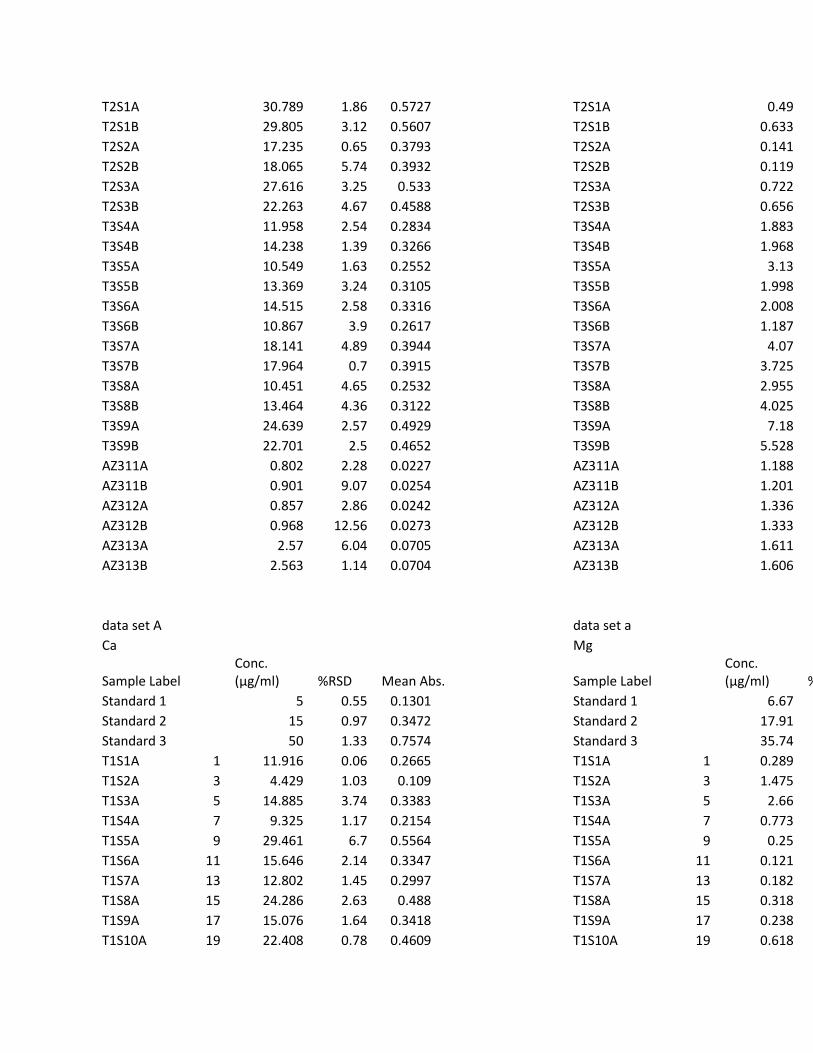
Sample Label Conc. (µg/ml) %RSD Mean Abs.

Full Calibration

Sample Label

Conc. (µg/ml) %RSD Mean Abs.

Table Blank ----- ----- 0 Standard 1 2.5 ----- 0.0652 Standard 2 5 ----- 0.1171 Standard 3 15 ----- 0.3259 T1S1A 11.916 0.06 0.2665 T1S1B 9.352 3.16 0.2159 T1S2A 4.429 1.03 0.109 T1-S2-B 5.481 2.94 0.133 2b

T1S3A

High 3.89 0.3992 T1S3B High 1.51 0.3642 T1S4A 9.325 1.17 0.2154 T1S4B 15.412 3.8 0.3306 STD 2.533 3.46 0.064 STD 5.173 1.07 0.1261 T1S5A High 0.41 0.6754 T1S5B High* 2.59 0.4118 T1S6A 15.646 2.14 0.3347 T1S6B High 1.53 0.3892 T1S7A High 0.61 0.3709 T1S7B High 1.49 0.3615 T1S8A High 0.92 0.5498 T1S8B High 1.79 0.6338 Analysis

Filename C:\Program Files\GBC Avanta Ver 1.33\Analysis1.anl

Element

Ca, Date Thu May 17 14:29:08 2012

Full Calibration Calibration Mode Conc Least Squares Max Error : 0.645 R² : 0.999

Full Calibration

Sample Label Conc. (µg/ml) %RSD Mean Abs.

Cal Blank ----- 0.9 0.0621 Standard 1 5 0.55 0.1301 Standard 2 15 0.97 0.3472 Standard 3 50 1.33 0.7574 Sample 2 2.613 0.35 0.0717 *

T1S3A 14.885 3.74 0.3383 T1S3B 12.971 0.88 0.3029 STD 47.478 1.97 0.7417 T1S5A 29.461 6.7 0.5564

T1S5B

15.785 1.05 0.3543 T1S6B 14.248 3.61 0.3268 T1S7A 12.802 1.45 0.2997 T1S7B 12.631 0.32 0.2964 T1S8A 24.286 2.63 0.488 T1S8B 28.437 1.41 0.5436 T1S9A 15.076 1.64 0.3418 STD 48.949 2.31 0.7541 T1S9B 7.787 6.82 0.1965 T1S10A 22.408 0.78 0.4609 T1S10B 22.068 1.4 0.4559 T1S11A 16.275 5.14 0.3629 T1S11B 17.371 0.65 0.3816 T1S12A 14.178 6.62 0.3255 T1S12B 13.84 3.78 0.3192

T2S1A

30.789 1.86 0.5727 T2S1B 29.805 3.12 0.5607 std 46.382 3.57 0.7323 T2S2A 17.235 0.65 0.3793 T2S2B 18.065 5.74 0.3932 T2S3A 27.616 3.25 0.533 T2S3B 22.263 4.67 0.4588 T3S4A 11.958 2.54 0.2834 T3S4B 14.238 1.39 0.3266

T3S5A 10.549 1.63 0.2552 T3S5B 13.369 3.24 0.3105 T3S6A 14.515 2.58 0.3316 std 49.25 0.35 0.7565 T3S6B 10.867 3.9 0.2617 T3S7A 18.141 4.89 0.3944

T3S7B

17.964 0.7 0.3915 T3S8A 10.451 4.65 0.2532 T3S8B 13.464 4.36 0.3122 T3S9A 24.639 2.57 0.4929 T3S9B 22.701 2.5 0.4652 AZ311A 0.802 2.28 0.0227 AZ311B 0.901 9.07 0.0254 std 40.556 8.72 0.6787 AZ312A 0.857 2.86 0.0242 AZ312B 0.968 12.56 0.0273 AZ313A 2.57 6.04 0.0705 AZ313B 2.563 1.14 0.0704 Analysis

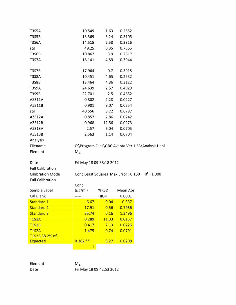
Filename C:\Program Files\GBC Avanta Ver 1.33\Analysis1.anl Element Mg,

Date

Fri May 18 09:38:18 2012 Full Calibration

Calibration Mode Conc Least Squares Max Error : 0.130 R² : 1.000 Full Calibration

Sample Label

Conc. (µg/ml) %RSD Mean Abs.

Cal Blank ----- HIGH 0.0001 Standard 1 6.67 0.04 0.337 Standard 2 17.91 0.56 0.7936 Standard 3 35.74 0.16 1.3496 T1S1A 0.289 11.33 0.0157 T1S1B 0.417 7.13 0.0226 T1S2A 1.475 0.74 0.0791 T1S2B 38.2% of

Expected 0.382 ** 9.27 0.0208

1

Element

Mg, Date Fri May 18 09:42:53 2012

Full Calibration Calibration Mode Conc Least Squares Max Error : 0.130 R² : 1.000

Full Calibration

Sample Label Conc. (µg/ml) %RSD Mean Abs.

Table Blank ----- ----- 0 Standard 1 6.67 ----- 0.337 Standard 2 17.91 ----- 0.7936 Standard 3 35.74 ----- 1.3496 T1S3A 2.66 0.37 0.1405 T1S3B 2.233 1.2 0.1186 T1S4A 0.773 1.14 0.0418 T1S4B 0.788 3.16 0.0426 STD 1.725 1.84 0.0922

T1S5A

0.25 1.45 0.0136 T1S5B 0.248 8.04 0.0135 T1S6A 0.121 16.5 0.0066 T1S6B 0.151 4.02 0.0082 T1S7A 0.182 8.77 0.0099 T1S7B 0.132 12.19 0.0072 T1S8A 0.318 7.34 0.0173 T1S8B 0.435 5.55 0.0236 T1S9A 0.238 5.3 0.013 STD 0.238 9.03 0.013 STD 6.894 0.69 0.3463 T1S9B 0.245 6.04 0.0134 T1S10A 0.618 1.76 0.0335 T1S10B 0.521 3.08 0.0283 T1S11A 0.551 4.93 0.0298 T1S11B 0.497 2.82 0.027 T1S12A 0.352 7.67 0.0192 T1S12B 0.338 6.03 0.0184 T2S1A 0.49 19.77 0.0266 T2S1B 0.633 4.87 0.0343 std 6.982 1.05 0.3504 T2S2A 0.141 8.04 0.0077 T2S2B 0.119 6.41 0.0065 T2S3A 0.722 3.44 0.039 T2S3B 0.656 1.23 0.0355 T3S4A 1.883 0.66 0.1004 T3S4A 1.91 2.63 0.1018 T3S4B 1.968 0.54 0.1048

T3S5A 3.13 0.52 0.1644 T3S5B 1.998 1.21 0.1064 T3S6A 2.008 0.67 0.1069 std 6.774 0.62 0.3408 T3S6B 1.187 1.57 0.0638 T3S7A 4.07 1.03 0.2114 T3S7B 3.725 0.48 0.1942 T3S8A 2.955 0.25 0.1555 T3S8B 4.025 1.12 0.2092 T3S9A 7.18 0.36 0.3595 T3S9B 5.528 0.82 0.2822 AZ311A 1.188 0.74 0.0639 AZ311B 1.201 2.88 0.0646 std 6.918 0.59 0.3475 AZ312A 1.336 1.61 0.0717 AZ312B 1.333 0.39 0.0716 AZ313A 1.611 0.41 0.0862 AZ313B 1.606 0.92 0.086 Analysis

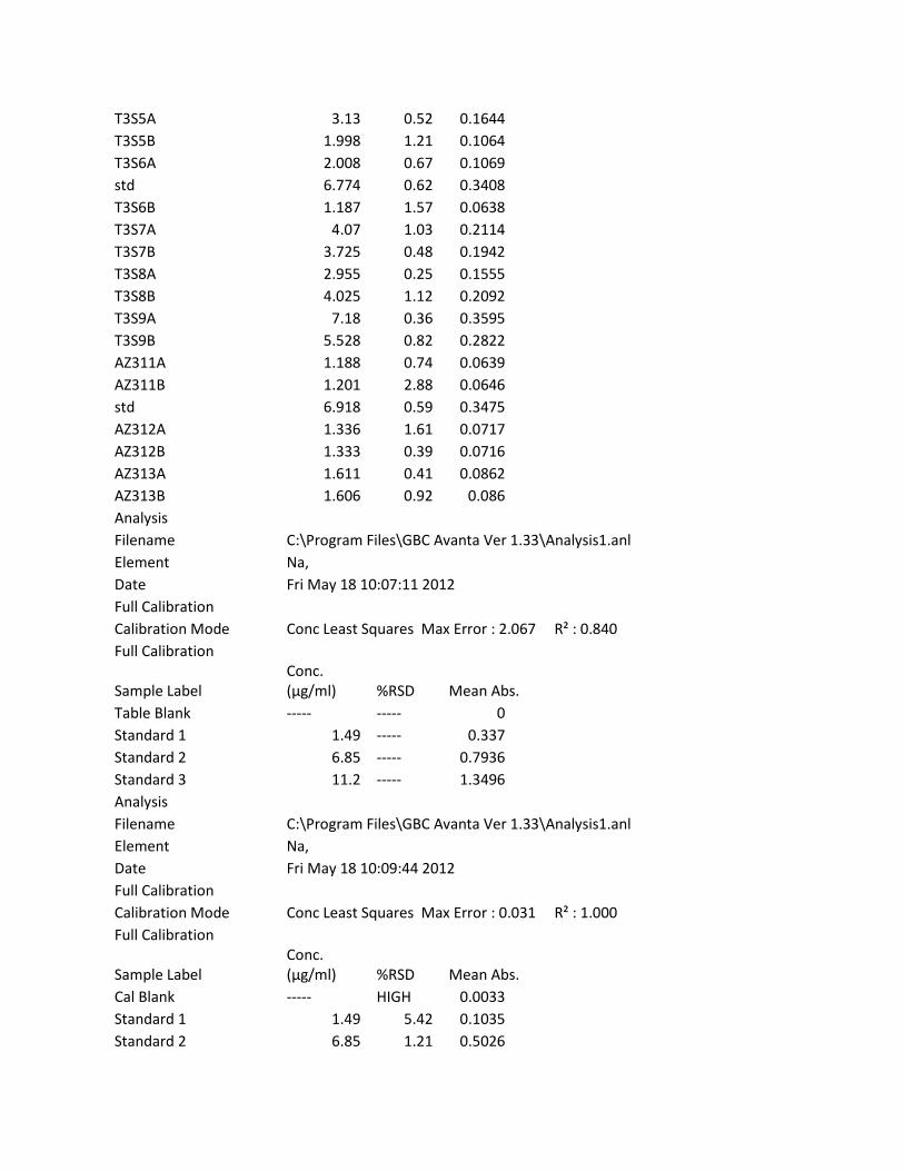
Filename C:\Program Files\GBC Avanta Ver 1.33\Analysis1.anl Element Na,

Date Fri May 18 10:07:11 2012 Full Calibration

Calibration Mode Conc Least Squares Max Error : 2.067 R² : 0.840 Full Calibration

Sample Label

Conc. (µg/ml) %RSD Mean Abs.

Table Blank ----- ----- 0 Standard 1 1.49 ----- 0.337 Standard 2 6.85 ----- 0.7936 Standard 3 11.2 ----- 1.3496 Analysis

Filename C:\Program Files\GBC Avanta Ver 1.33\Analysis1.anl Element Na,

Date Fri May 18 10:09:44 2012 Full Calibration

Calibration Mode Conc Least Squares Max Error : 0.031 R² : 1.000 Full Calibration

Sample Label

Conc. (µg/ml) %RSD Mean Abs.

Cal Blank ----- HIGH 0.0033 Standard 1 1.49 5.42 0.1035 Standard 2 6.85 1.21 0.5026

Standard 3 11.2 0.57 0.8497 T1S1A 1.294 1.83 0.0899 T1S1B High 0.25 1.631 T1S2A High HIGH 0.9389 Analysis

Filename C:\Program Files\GBC Avanta Ver 1.33\Analysis1.anl Element K,

Date Fri May 18 10:15:36 2012 Full Calibration

Calibration Mode Conc Least Squares Max Error : 0.303 R² : 0.995 Full Calibration

Sample Label

Conc. (µg/ml) %RSD Mean Abs.

Cal Blank ----- HIGH -0.0041 Standard 1 2.71 4.54 0.3058 Standard 2 4.57 ----- 0.5026 Standard 3 10.84 ----- 0.8497 Analysis

Filename C:\Program Files\GBC Avanta Ver 1.33\Analysis1.anl Element Na,

Date Tue May 22 10:47:20 2012 Full Calibration

Calibration Mode Conc Least Squares Max Error : 0.352 R² : 0.998 Full Calibration

Sample Label

Conc. (µg/ml) %RSD Mean Abs.

Cal Blank ----- 4.73 0.0152 Standard 1 6.85 ----- 0.3058 Standard 2 11.285 ----- 0.5026 Standard 3 22 ----- 0.8497 Analysis

Filename C:\Program Files\GBC Avanta Ver 1.33\Analysis1.anl Element Na,

Date Tue May 22 10:49:02 2012 Full Calibration

Calibration Mode Conc Least Squares Max Error : 0.548 R² : 0.996 Full Calibration

Sample Label

Conc. (µg/ml) %RSD Mean Abs.

Cal Blank ----- HIGH 0.002 Standard 1 6.85 1.44 0.3151 Standard 2 11.285 0.91 0.5798 Standard 3 22 0.69 1.1242

T1S1A 0.243 11.91 0.0112 T1S1B 2.395 1.15 0.1114 T1S2A High 0.55 1.3023 T1S2A 18.157 0.96 0.9226 20% multiply by 20

T1S2a 18.246 0.17 0.9276 20% dill T1S3A 0.282 15.76 0.013

T1S3B 0.177 HIGH 0.0081 T1S4A 2.047 0.79 0.0951 T1S4B 0.135 13.83 0.0062 STD 7.149 0.52 0.3413 T1S5A High 0.99 2.2512 30%

T1S5A 16.774 1.21 0.8455 30% dill multiply by 30 T1S5B 0.134 13.56 0.0061

T1S6A 0.191 18.37 0.0088 T1S6B 0.087 HIGH 0.004 T1S7A 0.92 15.35 0.0425 T1S7B 0.146 HIGH 0.0067 T1S8A 0.155 7.78 0.0071 T1S8B 0.28 HIGH 0.0129 T1S9A 0.076 HIGH 0.0035 STD 7.355 0.92 0.3515 T1S9B 0.99 2.14 0.0457 T1S10A 0.102 HIGH 0.0047 T1S10B 0.121 HIGH 0.0055 T1S11A 0.1 14.95 0.0046 T1S11B 0.096 HIGH 0.0044 T1S12A 0.072 HIGH 0.0033 T1S12B 0.136 18.2 0.0062 T2S1A 0.128 HIGH 0.0059 T2S1B 0.078 HIGH 0.0036 std 7.568 1.04 0.3621 T2S2A 0.133 5.73 0.0061 T2S2B 0 HIGH -0.0007 T2S3A 0.102 HIGH 0.0047 T2S3B 0.144 18.31 0.0066 T3S4A 0.444 4.01 0.0204 T3S4B 0.409 18.81 0.0188 T3S5A 1.362 2.42 0.063 T3S5B 1.527 1.71 0.0707 T3S6A 0.971 6.32 0.0448 std 7.728 1.67 0.3701 T3S6B 0.865 4.04 0.0399 T3S7A 1.421 1.01 0.0658

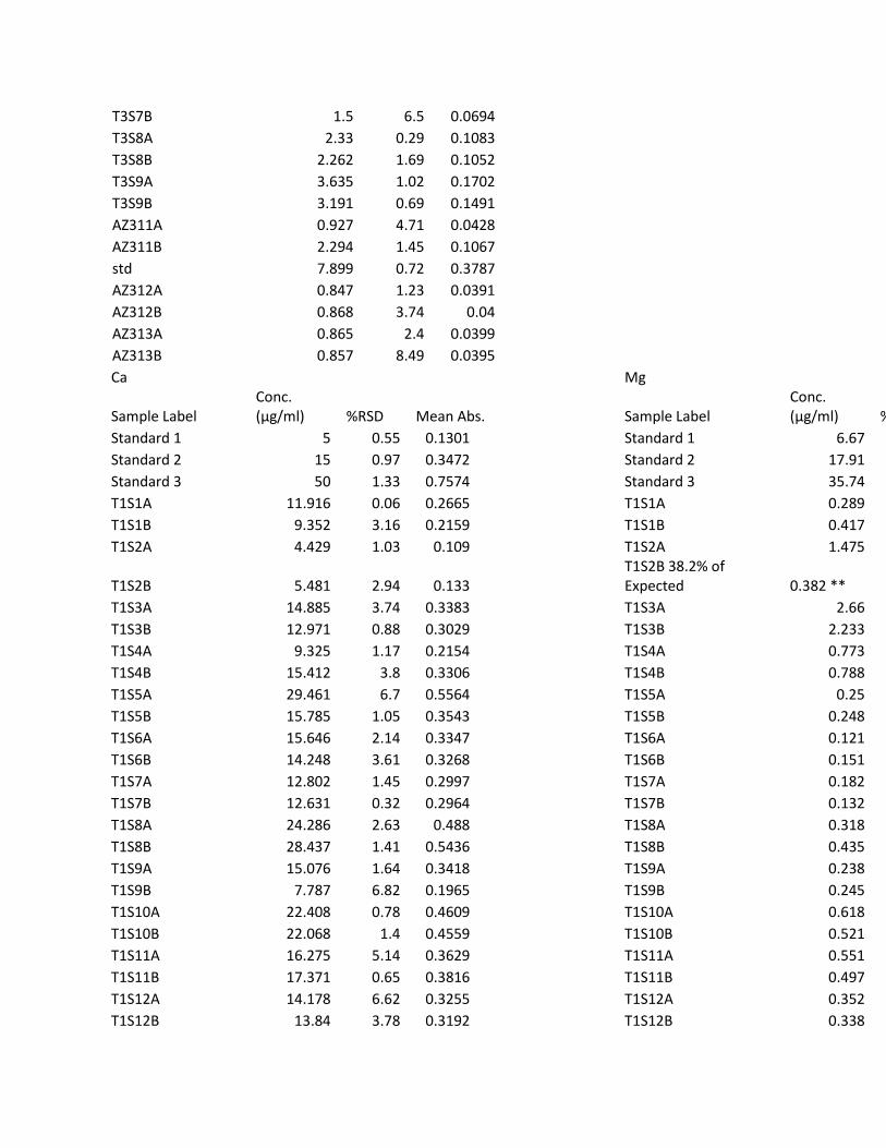
T3S7B 1.5 6.5 0.0694 T3S8A 2.33 0.29 0.1083 T3S8B 2.262 1.69 0.1052 T3S9A 3.635 1.02 0.1702 T3S9B 3.191 0.69 0.1491 AZ311A 0.927 4.71 0.0428 AZ311B 2.294 1.45 0.1067 std 7.899 0.72 0.3787 AZ312A 0.847 1.23 0.0391 AZ312B 0.868 3.74 0.04 AZ313A 0.865 2.4 0.0399 AZ313B 0.857 8.49 0.0395 Ca

Mg

Sample Label

Conc. (µg/ml) %RSD Mean Abs.

Sample Label

Conc. (µg/ml) %RSD

Mean Abs.

Standard 1 5 0.55 0.1301

Standard 1 6.67 0.04 0.337 Standard 2 15 0.97 0.3472

Standard 2 17.91 0.56 0.7936

Standard 3 50 1.33 0.7574

Standard 3 35.74 0.16 1.3496 T1S1A

11.916 0.06 0.2665

T1S1A

0.289 11.33 0.0157

T1S1B

9.352 3.16 0.2159

T1S1B

0.417 7.13 0.0226 T1S2A

4.429 1.03 0.109

T1S2A

1.475 0.74 0.0791

T1S2B

5.481 2.94 0.133

T1S2B 38.2% of Expected 0.382 ** 9.27 0.0208

T1S3A

14.885 3.74 0.3383

T1S3A

2.66 0.37 0.1405 T1S3B

12.971 0.88 0.3029

T1S3B

2.233 1.2 0.1186

T1S4A

9.325 1.17 0.2154

T1S4A

0.773 1.14 0.0418 T1S4B

15.412 3.8 0.3306

T1S4B

0.788 3.16 0.0426

T1S5A

29.461 6.7 0.5564

T1S5A

0.25 1.45 0.0136 T1S5B

15.785 1.05 0.3543

T1S5B

0.248 8.04 0.0135

T1S6A

15.646 2.14 0.3347

T1S6A

0.121 16.5 0.0066 T1S6B

14.248 3.61 0.3268

T1S6B

0.151 4.02 0.0082

T1S7A

12.802 1.45 0.2997

T1S7A

0.182 8.77 0.0099 T1S7B

12.631 0.32 0.2964

T1S7B

0.132 12.19 0.0072

T1S8A

24.286 2.63 0.488

T1S8A

0.318 7.34 0.0173 T1S8B

28.437 1.41 0.5436

T1S8B

0.435 5.55 0.0236

T1S9A

15.076 1.64 0.3418

T1S9A

0.238 5.3 0.013 T1S9B

7.787 6.82 0.1965

T1S9B

0.245 6.04 0.0134

T1S10A

22.408 0.78 0.4609

T1S10A

0.618 1.76 0.0335 T1S10B

22.068 1.4 0.4559

T1S10B

0.521 3.08 0.0283

T1S11A

16.275 5.14 0.3629

T1S11A

0.551 4.93 0.0298 T1S11B

17.371 0.65 0.3816

T1S11B

0.497 2.82 0.027

T1S12A

14.178 6.62 0.3255

T1S12A

0.352 7.67 0.0192 T1S12B

13.84 3.78 0.3192

T1S12B

0.338 6.03 0.0184

T2S1A

30.789 1.86 0.5727

T2S1A

0.49 19.77 0.0266 T2S1B

29.805 3.12 0.5607

T2S1B

0.633 4.87 0.0343

T2S2A

17.235 0.65 0.3793

T2S2A

0.141 8.04 0.0077 T2S2B

18.065 5.74 0.3932

T2S2B

0.119 6.41 0.0065

T2S3A

27.616 3.25 0.533

T2S3A

0.722 3.44 0.039 T2S3B

22.263 4.67 0.4588

T2S3B

0.656 1.23 0.0355

T3S4A

11.958 2.54 0.2834

T3S4A

1.883 0.66 0.1004 T3S4B

14.238 1.39 0.3266

T3S4B

1.968 0.54 0.1048

T3S5A

10.549 1.63 0.2552

T3S5A

3.13 0.52 0.1644 T3S5B

13.369 3.24 0.3105

T3S5B

1.998 1.21 0.1064

T3S6A

14.515 2.58 0.3316

T3S6A

2.008 0.67 0.1069 T3S6B

10.867 3.9 0.2617

T3S6B

1.187 1.57 0.0638

T3S7A

18.141 4.89 0.3944

T3S7A

4.07 1.03 0.2114 T3S7B

17.964 0.7 0.3915

T3S7B

3.725 0.48 0.1942

T3S8A

10.451 4.65 0.2532

T3S8A

2.955 0.25 0.1555 T3S8B

13.464 4.36 0.3122

T3S8B

4.025 1.12 0.2092

T3S9A

24.639 2.57 0.4929

T3S9A

7.18 0.36 0.3595 T3S9B

22.701 2.5 0.4652

T3S9B

5.528 0.82 0.2822

AZ311A

0.802 2.28 0.0227

AZ311A

1.188 0.74 0.0639 AZ311B

0.901 9.07 0.0254

AZ311B

1.201 2.88 0.0646

AZ312A

0.857 2.86 0.0242

AZ312A

1.336 1.61 0.0717 AZ312B

0.968 12.56 0.0273

AZ312B

1.333 0.39 0.0716

AZ313A

2.57 6.04 0.0705

AZ313A

1.611 0.41 0.0862 AZ313B

2.563 1.14 0.0704

AZ313B

1.606 0.92 0.086

data set A

data set a

Ca

Mg

Sample Label Conc. (µg/ml) %RSD Mean Abs.

Sample Label

Conc. (µg/ml) %RSD

Mean Abs.

Standard 1 5 0.55 0.1301

Standard 1 6.67 0.04 0.337 Standard 2 15 0.97 0.3472

Standard 2 17.91 0.56 0.7936

Standard 3 50 1.33 0.7574

Standard 3 35.74 0.16 1.3496 T1S1A 1 11.916 0.06 0.2665

T1S1A 1 0.289 11.33 0.0157

T1S2A 3 4.429 1.03 0.109

T1S2A 3 1.475 0.74 0.0791 T1S3A 5 14.885 3.74 0.3383

T1S3A 5 2.66 0.37 0.1405

T1S4A 7 9.325 1.17 0.2154

T1S4A 7 0.773 1.14 0.0418 T1S5A 9 29.461 6.7 0.5564

T1S5A 9 0.25 1.45 0.0136

T1S6A 11 15.646 2.14 0.3347

T1S6A 11 0.121 16.5 0.0066 T1S7A 13 12.802 1.45 0.2997

T1S7A 13 0.182 8.77 0.0099

T1S8A 15 24.286 2.63 0.488

T1S8A 15 0.318 7.34 0.0173 T1S9A 17 15.076 1.64 0.3418

T1S9A 17 0.238 5.3 0.013

T1S10A 19 22.408 0.78 0.4609

T1S10A 19 0.618 1.76 0.0335

T1S11A 21 16.275 5.14 0.3629

T1S11A 21 0.551 4.93 0.0298 T1S12A 23 14.178 6.62 0.3255

T1S12A 23 0.352 7.67 0.0192

T2S1A

30.789 1.86 0.5727

T2S1A

0.49 19.77 0.0266 T2S2A

17.235 0.65 0.3793

T2S2A

0.141 8.04 0.0077

T2S3A

27.616 3.25 0.533

T2S3A

0.722 3.44 0.039 T3S4A 1 11.958 2.54 0.2834

T3S4A 1 1.883 0.66 0.1004

T3S5A 3 10.549 1.63 0.2552

T3S5A 3 3.13 0.52 0.1644 T3S6A 5 14.515 2.58 0.3316

T3S6A 5 2.008 0.67 0.1069

T3S7A 7 18.141 4.89 0.3944

T3S7A 7 4.07 1.03 0.2114 T3S8A 9 10.451 4.65 0.2532

T3S8A 9 2.955 0.25 0.1555

T3S9A 11 24.639 2.57 0.4929

T3S9A 11 7.18 0.36 0.3595 AZ311A

0.802 2.28 0.0227

AZ311A

1.188 0.74 0.0639

AZ312A

0.857 2.86 0.0242

AZ312A

1.336 1.61 0.0717 AZ313A

2.57 6.04 0.0705

AZ313A

1.611 0.41 0.0862

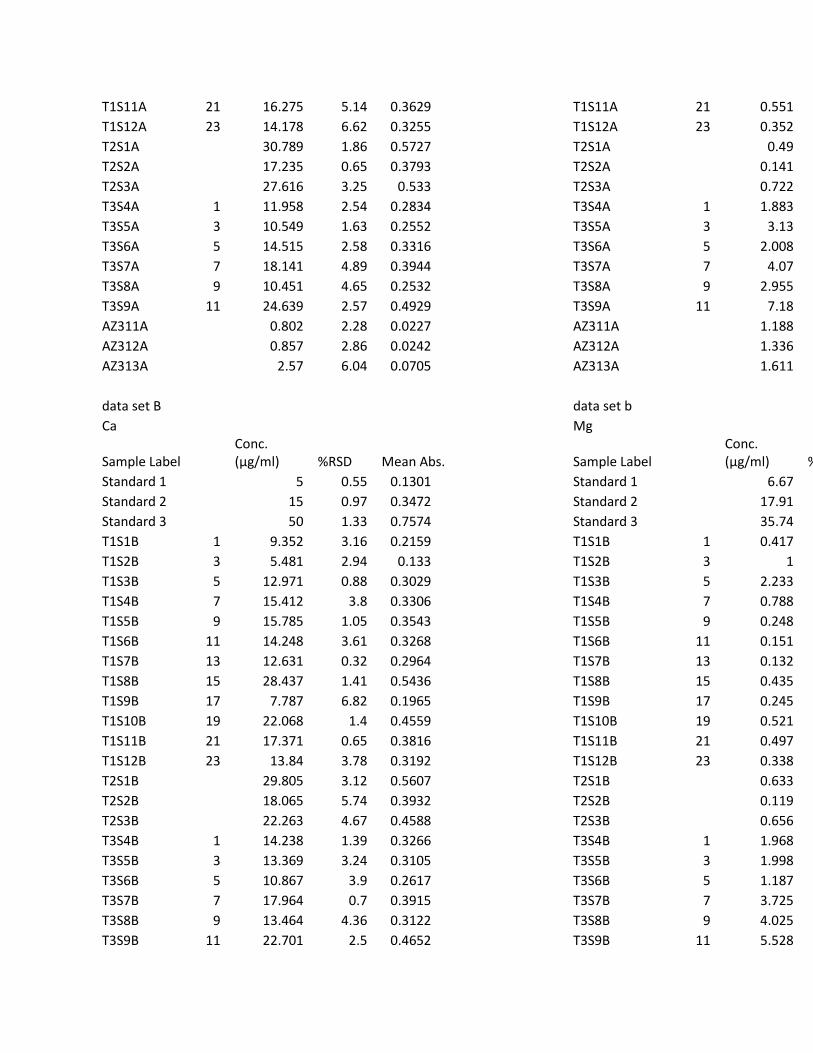
data set B

data set b Ca

Mg

Sample Label

Conc. (µg/ml) %RSD Mean Abs.

Sample Label

Conc. (µg/ml) %RSD

Mean Abs.

Standard 1 5 0.55 0.1301

Standard 1 6.67 0.04 0.337 Standard 2 15 0.97 0.3472

Standard 2 17.91 0.56 0.7936

Standard 3 50 1.33 0.7574

Standard 3 35.74 0.16 1.3496 T1S1B 1 9.352 3.16 0.2159

T1S1B 1 0.417 7.13 0.0226

T1S2B 3 5.481 2.94 0.133

T1S2B 3 1 9.27 0.0208 T1S3B 5 12.971 0.88 0.3029

T1S3B 5 2.233 1.2 0.1186

T1S4B 7 15.412 3.8 0.3306

T1S4B 7 0.788 3.16 0.0426 T1S5B 9 15.785 1.05 0.3543

T1S5B 9 0.248 8.04 0.0135

T1S6B 11 14.248 3.61 0.3268

T1S6B 11 0.151 4.02 0.0082 T1S7B 13 12.631 0.32 0.2964

T1S7B 13 0.132 12.19 0.0072

T1S8B 15 28.437 1.41 0.5436

T1S8B 15 0.435 5.55 0.0236 T1S9B 17 7.787 6.82 0.1965

T1S9B 17 0.245 6.04 0.0134

T1S10B 19 22.068 1.4 0.4559

T1S10B 19 0.521 3.08 0.0283 T1S11B 21 17.371 0.65 0.3816

T1S11B 21 0.497 2.82 0.027

T1S12B 23 13.84 3.78 0.3192

T1S12B 23 0.338 6.03 0.0184 T2S1B

29.805 3.12 0.5607

T2S1B

0.633 4.87 0.0343

T2S2B

18.065 5.74 0.3932

T2S2B

0.119 6.41 0.0065 T2S3B

22.263 4.67 0.4588

T2S3B

0.656 1.23 0.0355

T3S4B 1 14.238 1.39 0.3266

T3S4B 1 1.968 0.54 0.1048 T3S5B 3 13.369 3.24 0.3105

T3S5B 3 1.998 1.21 0.1064

T3S6B 5 10.867 3.9 0.2617

T3S6B 5 1.187 1.57 0.0638 T3S7B 7 17.964 0.7 0.3915

T3S7B 7 3.725 0.48 0.1942

T3S8B 9 13.464 4.36 0.3122

T3S8B 9 4.025 1.12 0.2092 T3S9B 11 22.701 2.5 0.4652

T3S9B 11 5.528 0.82 0.2822

AZ311B

0.901 9.07 0.0254

AZ311B

1.201 2.88 0.0646 AZ312B

0.968 12.56 0.0273

AZ312B

1.333 0.39 0.0716

AZ313B

2.563 1.14 0.0704

AZ313B

1.606 0.92 0.086 Na

new

Sample Label

Conc. (µg/ml)

Conc. (µg/ml) %RSD

Mean Abs.

Standard 1 6.85 1.44 0.3151 Standard 2 11.285 0.91 0.5798 Standard 3 22 0.69 1.1242 T1S1A

0.243 11.91 0.0112

T1S1B

2.395 1.15 0.1114 T1S2A

18.157 0.96 0.9226 0.2

T1S2a

18.246 0.17 0.9276 20% dill T1S3A

0.282 15.76 0.013

T1S3B

0.177 HIGH 0.0081 T1S4A

2.047 0.79 0.0951

T1S4B

0.135 13.83 0.0062 T1S5A

16.774 1.21 0.8455 0.3

T1S5B

0.134 13.56 0.0061 30% dill T1S6A

0.191 18.37 0.0088

T1S6B

0.087 HIGH 0.004 T1S7A

0.92 15.35 0.0425

T1S7B

0.146 HIGH 0.0067 T1S8A

0.155 7.78 0.0071

T1S8B

0.28 HIGH 0.0129 T1S9A

0.076 HIGH 0.0035

T1S9B

0.99 2.14 0.0457 T1S10A

0.102 HIGH 0.0047

T1S10B

0.121 HIGH 0.0055 T1S11A

0.1 14.95 0.0046

T1S11B

0.096 HIGH 0.0044 T1S12A

0.072 HIGH 0.0033

T1S12B

0.136 18.2 0.0062 T2S1A

0.128 HIGH 0.0059

T2S1B

0.078 HIGH 0.0036 T2S2A

0.133 5.73 0.0061

T2S2B

0 HIGH -0.0007 T2S3A

0.102 HIGH 0.0047

T2S3B

0.144 18.31 0.0066 T3S4A

0.444 4.01 0.0204

T3S4B

0.409 18.81 0.0188 T3S5A

1.362 2.42 0.063

T3S5B

1.527 1.71 0.0707

T3S6A

0.971 6.32 0.0448 T3S6B

0.865 4.04 0.0399

T3S7A

1.421 1.01 0.0658 T3S7B

1.5 6.5 0.0694

T3S8A

2.33 0.29 0.1083 T3S8B

2.262 1.69 0.1052

T3S9A

3.635 1.02 0.1702 T3S9B

3.191 0.69 0.1491

AZ311A

0.927 4.71 0.0428 AZ311B

2.294 1.45 0.1067

AZ312A

0.847 1.23 0.0391 AZ312B

0.868 3.74 0.04

AZ313A

0.865 2.4 0.0399 AZ313B

0.857 8.49 0.0395

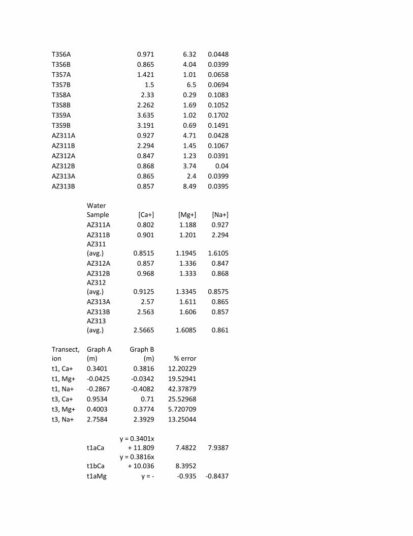
Water Sample [Ca+] [Mg+] [Na+]

AZ311A 0.802 1.188 0.927

AZ311B 0.901 1.201 2.294

AZ311 (avg.) 0.8515 1.1945 1.6105

AZ312A 0.857 1.336 0.847

AZ312B 0.968 1.333 0.868

AZ312 (avg.) 0.9125 1.3345 0.8575

AZ313A 2.57 1.611 0.865

AZ313B 2.563 1.606 0.857

AZ313 (avg.) 2.5665 1.6085 0.861

Transect, ion

Graph A (m)

Graph B (m) % error

t1, Ca+ 0.3401 0.3816 12.20229 t1, Mg+ -0.0425 -0.0342 19.52941 t1, Na+ -0.2867 -0.4082 42.37879 t3, Ca+ 0.9534 0.71 25.52968 t3, Mg+ 0.4003 0.3774 5.720709 t3, Na+ 2.7584 2.3929 13.25044

t1aCa

y = 0.3401x + 11.809 7.4822 7.9387

t1bCa

y = 0.3816x + 10.036 8.3952

t1aMg y = - -0.935 -0.8437

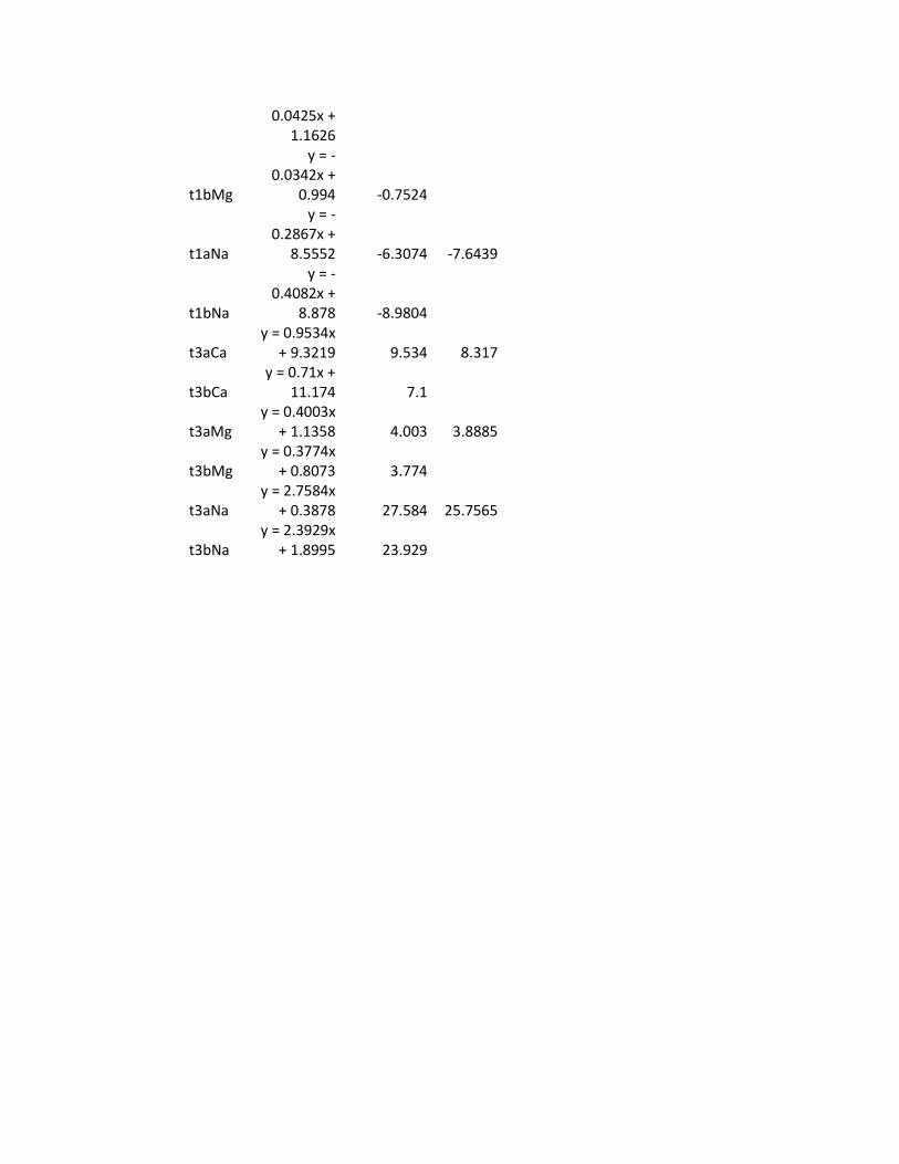
0.0425x + 1.1626

t1bMg

y = -0.0342x +

0.994 -0.7524

t1aNa

y = -0.2867x +

8.5552 -6.3074 -7.6439

t1bNa

y = -0.4082x +

8.878 -8.9804

t3aCa

y = 0.9534x + 9.3219 9.534 8.317

t3bCa

y = 0.71x + 11.174 7.1

t3aMg

y = 0.4003x + 1.1358 4.003 3.8885

t3bMg

y = 0.3774x + 0.8073 3.774

t3aNa

y = 2.7584x + 0.3878 27.584 25.7565

t3bNa

y = 2.3929x + 1.8995 23.929