Economic Research Southern Africa (ERSA) is a research programme funded by the National Treasury of South Africa. The views expressed are those of the author(s) and do not necessarily represent those of the funder, ERSA or the author’s affiliated institution(s). ERSA shall not be liable to any person for inaccurate information or opinions contained herein. The analysis of borders effects in intra- African trade Emilie Kinfack Djoumessi and Alain Pholo Bala ERSA working paper 701 August 2017

Welcome message from author
This document is posted to help you gain knowledge. Please leave a comment to let me know what you think about it! Share it to your friends and learn new things together.
Transcript
Economic Research Southern Africa (ERSA) is a research programme funded by the National
Treasury of South Africa. The views expressed are those of the author(s) and do not necessarily represent those of the funder, ERSA or the author’s affiliated
institution(s). ERSA shall not be liable to any person for inaccurate information or opinions contained herein.
The analysis of borders effects in intra-
African trade
Emilie Kinfack Djoumessi and Alain Pholo Bala
ERSA working paper 701
August 2017
The analysis of borders effects in intra-African trade
Emilie Kinfack Djoumessi∗ Alain Pholo Bala ∗†
August 23, 2017
Abstract
The study aims to analyze the border effects on intra–African trade through the use of a gravity
specification based on the monopolistic competition model of trade introduced by Krugman (1980).
The study used CEPII data on trade flows between African countries over the period 1980-2006.
We accommodate for the significant number of zero trade flows between several African countries
by using the Heckman correction method. The findings suggest that while the extent of market
fragmentation is on average very high within the African continent, the border effects within SADC
and ECOWAS are more in line with other international estimations. Whereas results indicate that
border effects faced by intra-African trade are quite substantial: on average an African country trade
108 times more “with itself” than with another country on the continent. Border effects in SADC
and ECOWAS are respectively about 5 and 3 times lower. The inclusion of the infrastructure indices
contributes significantly to this result. Considering infrastructure is actually an interesting way to
capture the effect of distribution networks which represent, along with imperfect information and
localized tastes, relevant but generally omitted sources of resistance.
Keyword: Intra-African Trade, Monopolistic Competition Model, Border Effect
JEL Classification: F12, F14, F15
1 Introduction
The analysis of economic growth in sub-Saharan Africa (SSA) has raised some major concerns in the De-
velopment Economics literature (Collier, 2006a,b; Dollar and Easterly, 1999; Easterly and Levine, 1997;
Easterly, 2009a,b). While this continent has experienced strong economic growth rates lately (Pinkovskiy
and Sala-i Martin, 2014), until the 1990s SSA was characterized by low and even sometimes negative
∗Department of Economics & Econometrics, University of Johannesburg, APK Campus, PO Box 524, Auckland Park
2006, Johannesburg, South Africa.†Public and Environmental Economics Research Centre (PEERC), Corresponding author. E-mail address:
1
economic growth (Cinyabuguma and Putterman, 2011; Easterly and Levine, 1997; Sachs and Warner,
1997; Artadi and Sala-i Martin, 2003).
Several impediments specific to the African growth process have been identified. Among them, we
may consider that SSA is badly affected by low population density, long distances and high fragmenta-
tion (World Bank, 2008). High transport costs add to the high fragmentation of that region. For goods
to pass the border in Africa, it takes more than 40 days which is twice the period in Latin America.
The constraints are even worse for landlocked countries (Freire et al., 2015).
Collier (2006a) asserts that agglomeration economies in SSA are less important than those prevailing
in Asia and in OECD countries. Because countries in that region are too small and not integrated
enough, many African cities tend to be too small compared to the optimum. As shown by Au and
Henderson (2006) in the case of Asia, this may have serious impacts in terms of foregone growth.
Research on agglomeration economies and international competitiveness further suggests that late-
comers to industrialization, such as Africa’s natural resource exporters, face a competitive disadvantage
linked to the spatial distribution of the global industry (Page, 2008).
Africa appears as fragmented and poorly integrated. Intra-regional trade in the region is fairly low
comparatively to what is noticed in other areas. Therefore, improving regional integration appears as
one of the key strategies that might foster economic growth in the African continent. Better regional
integration might help SSA achieve greater economies of scale, widen markets, enhance industrial effi-
ciency, and reduce the sub-region’s external dependency and vulnerability of its economy (Jones, 2002).
The other benefits that may be expected from an increased regional integration are the following: a
greater bargaining power vis-a-vis the outside world; the minimization of duplication; thin spreading of
resources and wasteful competition; a cheaper and more efficient transportation system; greater divi-
sion of labor and specialization in production; established and strengthened product value chains and
facilitated transfer of technology and knowledge via spillover effects; expansion of trade, incomes and
employment due to free movement of goods, services, labor and capital, etc. (Jones, 2002; UNECA,
2010).
Another argument exists for promoting intra-African trade. To take advantage of trade-growth
opportunities, SSA is prompted to diversify in several ways: one way would be by reducing its reliance
on the stagnating markets of its traditional trading partners from the Organisation for Economic Co-
operation and Development (OECD). Concurrently, it needs to become less dependent on the export of
commodities vulnerable to price shocks (ITC, 2012). The redirection of SSA exports towards Asia, and
China in particular, is already underway. However, since the large majority of SSA products destined
for Asia are commodities, such a reorientation to growth markets does not eradicate the vulnerability to
commodity price shocks. SSA countries increasingly trade within their own region too. This new trend
of SSA trade is likely to achieve sustainability in export revenues by integrating deeper into sector value-
chains and in this way increasing the share of value-added products within its exports. The redirection
of SSA exports towards Africa may further reduce the risks caused by the volatility of commodity price
2
shocks.
However, despite Africa’s commitment to ease trade restrictions in order to create a common market
within the framework of Regional Economic Communities (RECs) and the reorientation of its trade,
barriers to intra-African trade tend to persist. On average over the past decade, only about 10%-12%
of African trade has been with African nations, while 40% of North American trade has been with
other North American countries, and 63% of trade in Western Europe is with other Western European
nations (Economic Commission for Africa, 2011). Intra-African trade is also low when compared to
that of other developing regions; intra Latin America trade amounts to 20 % while trade within Asian
developing countries represents 48 % (Ancharaz et al., 2011). In this regard, SSA’s trade seems to be
extroverted as a substantial share of it is directed to the developed world: in 2011 more than half of
SSA’s merchandise trade was still done with the OECD partners (ITC, 2012).
The orientation of most of African trade towards developed partners raises the issue of the effec-
tiveness of trade integration policies throughout African countries and RECs. In this paper, we assess
the effectiveness of the strategies adopted by African countries and regional groupings to foster trade
integration. We do so by evaluating the extent of border effects in intra-African trade. The intensity of
border effects helps to characterize the extent of market fragmentation. The term “border effect” refers
to the downward impact of national boundaries on the volume of trade, i.e. that two different countries
trade far less with each other than do two locations in the same country, after controlling for factors such
as income, alternative trading opportunities, distance, languages, and regional trade agreements (Evans,
2003). Markets are considered fragmented when national borders influence the pattern of commercial
transactions (Head and Mayer, 2000).
Using border effects to measure the extent of market fragmentation is more robust than using market
shares. As pointed out by de Sousa et al. (2012), while they are insightful, the market shares referred
to above cannot be sufficient to draw conclusions on the level of market fragmentation faced by African
exporters on the intra-regional market. The first problem is that any assessment of market access based
on trade flows needs to specify a benchmark of trade patterns, to which actual international exchanges
of goods will be compared. Without such a benchmark, which can only be provided by theory, we do
not know what to compare those numbers to. This need of a reference for comparison justifies why we
will derive an empirically estimable gravity-type equation from a theoretical framework.
A second limitation implied by the use of the import shares to assess market access is that for most
products, the large majority of overall demand in a country is met by domestic producers, not foreign.
A more relevant index of market access must take into account the market share of foreign producers
in the overall demand. This is precisely what the border effects method does. The method considers
trade flows within countries as well as among countries and compares imports from foreign countries to
“imports from self” of domestic producers. Hence, this approach gives a benchmark based on a situation
of the best possible market access, the one faced by domestic producers (de Sousa et al., 2012).
Border effects matter when firms have greater access to domestic consumers than to consumers in
3
other nations. Following Head and Mayer (2000), we measure border effects as the average spread be-
tween actual trade and the trade that would be expected in an economy without border-related barriers.
To capture border effects we rely on a gravity model. The gravity model offers a powerful empirical
framework for analyzing bilateral trade flows (Anderson and van Wincoop, 2003; Behrens et al., 2012).
However, the specification of gravity models has improved significantly over time. With an ad hoc spec-
ification linking bilateral trade flows to importer and exporter GDP and bilateral distance, McCallum
(1995) found an impressive border effect between the Canadian provinces and the United States, i.e.
the trade between two provinces is more than 20 times larger than trade between a province and an
American state. These findings, which were confirmed by Helliwell (1996) and Hillberry (1998), suggest
a very large degree of home bias in trade within North-America . One of the implication of the so-called
“border puzzle” would be that international trade flows would remain much less dense than national
trading ties even after all tariffs were removed.
However, some serious concerns have been raised on this first wave of studies. Anderson and van
Wincoop (2003) pointed out that the lack of theoretical foundation of gravity equations has two adverse
consequences. First, estimation results are likely to be biased because of omitted variables. Second, it
is not possible to conduct a comparative statics exercise. Therefore, Anderson and van Wincoop (2003)
used an estimated general equilibrium model to solve the “border puzzle”. Anderson and van Wincoop
(2003)’s model modifies McCallum (1995)’s specification by adding “multilateral resistance” variables.
Applying their model to 1993 data, Anderson and van Wincoop (2003) found only moderate impact of
trade barriers on trade flows: borders reduce trade between USA and Canada by 44%, and trade among
other industrialized countries by 29%.
In this paper, we follow Head and Mayer (2000) and Combes et al. (2005) by performing a structural
estimation based on the monopolistic competition model of trade proposed by Krugman (1980). That
Krugman model derives a relation between the relative amounts consumers spend on foreign and domes-
tic goods and their relative prices. The border effect is captured by the divergence between actual and
predicted consumption ratios. The remainder of the paper is organized as follows. Section 2 presents
the theoretical model and the implied econometric specifications. The data are described in Section 3.
And finally, the econometric results are given in Section 4.
2 Model
Several theory-consistent estimation methods for the gravity model exist (Head and Mayer, 2013a). With
the data at hand, bilateral trade flow between countries per industry, we can estimate border effects
only through the complete odds specification as in Head and Mayer (2000) and Combes et al. (2005).1
Therefore, we follow Head and Mayer (2000)’s and Combes et al. (2005)’s approach of including border
effects into a monopolistic competition model. We use a fairly broad specification of preferences. The
utility of the representative consumer in country i depends on the quantity of each variety h consumed
4
from each country j. We assume that all varieties are differentiated from each other but products from
the same country are weighted equally in the utility function. Representing the quantity consumed with
c and the preference weight with a, the constant elasticity of substitution utility function is given by:
Ui =
N∑j=1
nj∑h=1
(aijcijh)σ−1σ
σσ−1
, (1)
while the implied budget constraint is
Yi =N∑j=1
nj∑h=1
pijhcijh (2)
We may simplify the consumer optimization problem by assuming that all quantities of the varieties
imported by country i from country j are symmetric. Then, denoting mij as the CIF value of exports
from country j to country i (mij = njcijpij) and mi =
N∑k=1
mik as expenses on goods from all origins
(including the home country), one may obtain the following expression of bilateral imports after some
algebra
mij =njp
1−σij aσ−1
ij
N∑k=1
nkp1−σik aσ−1
ik
mi. (3)
2.1 Econometric specifications
A gravity equation may be derived from this expression and may lead to different econometric specifi-
cations. As the number of symmetric varieties is not observed, we may eliminate nj and nk in equation
(3) by substituting them from equation (4)
νj = qpjnj (4)
where νj denotes the value of production in country j, q represents the quantity produced by each firm
and pj denotes the mill price of each variety. Considering the determination of delivered prices, pij , and
of preferences, aij , we assume that the price paid by consumers in country i for products of country j
is the product of the mill price, pj , and of transaction costs Tij
pij = pjTij (5)
We model transaction costs as a multiplicative function of the distance dij ; of the bilateral industry
level tariffs τij ; of the Non Tariffs Barriers (NTBs); of the level of infrastructure of the country i (j)
(INi(j)), and of an exponential function involving a contiguity dummy Cij . Furthermore, we assume
constant ad valorem NTBs of ξ for all cross-border trade. Defining Bij as a dummy variable taking a
5
value of one for i 6= j, we obtain
Tij = dδ1ij tδ2ij
[(1 + ξ) INi
−δ3INj−δ4e−δ5Cij
]Bij, (6)
with the tariff factor tij expressed as tij = 1 + τij .
Consumer preferences consist of a stochastic component, εij , and a systematic preference for home-
produced goods (or aversion to foreign-made goods) of α. Moreover, we hypothesize that several vari-
ables may mitigate or accentuate home bias and therefore posit the following equation for preferences:
aij = exp[εij −
(α− β1Lij − β2Eij − β3COLij + β4Vij −R′ijφ
)Bij]
(7)
where Lij takes the value of one for pairs of countries that share a common official language, and zero
otherwise; Eij takes the value of 1 when a language is spoken by at least 9% of the population in both
countries i and j (ethnic language); COLij = 1 if countries i and j had a common colonizer; and Vij is
the volatility of the bilateral exchange rate between countries i and j. Rij depicts a vector composed
of indicator variables taking the value of one when both countries i and j belong to the same regional
groupings like SADC, ECOWAS, and COMESA or if countries i and j had a common colonizer after
1945; while φ is the corresponding vector of parameters. Substituting for aij , pij and nj in (3) and
taking logs we obtain the formulation of the gravity equation:
lnmij = lnmi + ln νj − (σ − 1) δ1 ln dij − (σ − 1) δ2 ln tij − σ ln pj − Ii (8)
− (σ − 1)[α− β1Lij − β2Eij − β3COLij + β4Vij −R′ijφ+ ln (1 + ξ)− δ3 ln INi − δ4 ln INj
− δ5Cij ]Bij + (σ − 1) εij
where Ii depicts the Head and Mayer (2000) importer’s “inclusive value” defined as follows:
Ii = ln
{N∑k=1
exp [ln νk − σ ln pk + (σ − 1) (−δ1 ln dik − δ2 ln tik + εik
−[α− β1Lik − β2Eik − β3COLik + β4Vik −R′ikφ+ ln (1 + ξ) + δ3 ln INi + δ4 ln INk − δ5Cik
]Bik)]}
The inclusive value captures the impact of the full range of potential suppliers to a given importer
by taking into account their size, distance and relative border effects. There are several problems in
estimating the influence of Ii (Head and Mayer, 2000). The most critical is that such an estimation
would rely on parameters that are already in the equation to be estimated. There are two ways of
sidestepping those problems. First, we may derive from equation (8) a fixed-effects specification fully
consistent with theory. An alternative specification is to define a complete odds specification by setting
j = i in (8) to obtain an expression for ln (mii), then to subtract ln (mii) from ln (mij).
As in Combes et al. (2005) and in the spirit of Hummels (1999) and Redding and Venables (2004),
6
it is possible to derive from equation (8) a fixed-effects specification fully consistent with our theoretical
model. This derivation implies replacing all destination-specific and origin-specific variables by two
groups of destination and origin fixed effects. Only variables varying both with origin and destination
are left in the regression.
However, this approach has several problems. First, it does not permit the estimation of all structural
parameters. In particular, σ the elasticity of substitution between varieties cannot be recovered. Second,
as the approach implies dropping internal trade flows, it approach excludes the possibility of estimating
border effects. Therefore, to be able to estimate structural parameters and to evaluate border effects
we rely on the complete odds specification.
2.2 The complete odds specification
Setting j = i in (8) to obtain an expression for ln (mii) and then, subtracting ln (mii) from ln (mij), we
obtain the following complete odds specification (Combes et al., 2005):
ln
(mij
mii
)= − (σ − 1) [α+ ln (1 + ξ)] + ln
(νjνi
)− σ ln
(pjpi
)− (σ − 1) δ1 ln
(dijdii
)− (σ − 1) δ2 ln tij + (σ − 1) δ3 ln INi + (σ − 1) δ4 ln INj + (σ − 1) δ5Cij (9)
+ (σ − 1)β1Lij + (σ − 1)β2Eij + (σ − 1)β3COLij − (σ − 1)β4Vij + (σ − 1)R′ijφ+ εij
where εij = (σ − 1) (εij − εii). This expression of the error term implies that errors are not independently
distributed. We account for this correlation in the estimation through a robust procedure, allowing
residuals of the same importing region to be correlated.
In other words, according to (9) the log of odds ratios is expected to increase with the log of relative
production ln(νjνi
), with the fact that both importer and exporter share common languages and had a
common colonizer after 1945 and to decrease with the logs of relative distance, ln(dijdii
), tariffs factor,
ln (1 + τij), bilateral exchange rate volatility Vij and relative price, ln(pjpi
).
The intercept in (9) may be described as the border effect. It is the average deviation between actual
trade and the trade that would be expected in an economy without border-related barriers. It clearly
captures the impact of NTBs (ξ) and home bias (α) as in Head and Mayer (2000).
Equation (9) implies a unit elasticity on relative production; thus it may be rewritten as
ln
(mij
mii
)− ln
(νjνi
)= − (σ − 1) [α+ ln (1 + ξ)]− σ ln
(pjpi
)− (σ − 1) δ1 ln
(dijdii
)− (σ − 1) δ2 ln tij + (σ − 1) δ3 ln INi + (σ − 1) δ4 ln INj + (σ − 1) δ5Cij (10)
+ (σ − 1)β1Lij + (σ − 1)β2Eij + (σ − 1)β3COLij − (σ − 1)β4Vij + (σ − 1)R′ijφ+ εij
Imposing a unit elasticity on relative production helps addressing two different econometric issues:
7
first, output and trade are jointly determined in equilibrium (Harrigan, 1996; Head and Mayer, 2000);
which entails an endogeneity problem. Moving relative production in the left-hand side as in (10) is a
way to handle this simultaneity issue without resorting to instrumental variables. This strategy may
address another problem: measurement error for production. As production information may be inexact
especially for developing countries of SSA, we may obtain biased coefficients estimates.
2.3 Heckman correction for sample selection bias
The monopolistic competition trade model assumes positive trade between each country pair in each
industry (Head and Mayer, 2000). More generally, most of the structural gravity models do not naturally
generate zero flows (Head and Mayer, 2013a). However, most trade data sets exhibit substantial fractions
of zeros (Head and Mayer, 2013a). Helpman et al. (2008) show that, at the country level, country pairs
that do not trade with each other or trade in only one direction account for about half the observations.
There are two implications of a prevalence of zeros (Head and Mayer, 2013a). First, trade models need
to be adjusted in order to accommodate zeros. Second, estimation methods should be revised to allow
for consistent estimates in the presence of a dependent variable having a high incidence of zeros.
Several approaches can be used to accommodate structural gravity models to a prevalence of ze-
ros (Head and Mayer, 2013a). One simple approach is to consider that zeros arise from a data recording
issue, that is “there are no “structural zeros” but only “statistical zeros”” (Head and Mayer, 2013a,
p. 50-51). Some structural models generate zeros endogenously by adding a fixed cost of exporting from
i to j (Helpman et al., 2008; Eaton et al., 2012).2 These models have the common characteristic that
zeros are more likely between small and/or distant countries (Baldwin and Harrigan, 2011; Head and
Mayer, 2013a). As log of zero is not defined, observations without positive bilateral trade are lost, which
results in systematic selection bias as shown in Head and Mayer (2013a).
To find out which estimators may be consistent when zeros are an endogenous component of the data-
generating process, Head and Mayer (2013a) compare several estimators with a Monte Carlo Simulation:
the Least Squares Dummy Variables (LSDV), the Eaton and Tamura (1994) (ET) Tobit model, the Eaton
and Kortum (2001) (EK) Tobit model, the Multinomial Pseudo-Maximum-Likelihood (Multinomial
PML), the Poisson PML and the Gamma PML. The main findings of this Monte Carlo simulation
exercise is that the choice of the most suitable estimator depends on the process generating the error
term. Under the Constant Variance to Mean Ratio (CVMR) assumption, Poisson or Multinomial PML
provide the best estimators. However, under the log-normality assumption the EK Tobit method should
be preferred.
The Heckman selection model was left out of the Monte Carlo simulation exercise. The reason
advanced by Head and Mayer (2013a) is that the method used by Helpman et al. (2008), the leading
paper using a Heckman based approach of zeros, is designed to uncover a different set of parameters
than the other approaches which estimate coefficients that combine extensive and intensive margins.
The critical challenge implied by the Heckman-based methods is the difficulty of finding an exclusion
8
restriction. One would preferably use a variable in the probit selection equation which according to the
theory can be excluded from the gravity regression equation. Since both equations have exporter and
importer invariant variables, this variable should be dyadic in nature (Head and Mayer, 2013a).
Given, the poor results obtained with the EK Tobit and the Poisson PML, in this paper we fol-
low Head and Mayer (2000) who used a two-step Heckman selection model for a complete odds specifi-
cation.3 For the exclusion restriction we follow Helpman et al. (2008) by using two indicators for high
entry barriers in both countries i and j. These entry costs are captured through their effects on the
number of days, the number of legal procedures, and the relative cost (as a percentage of GDP per
capita) for an entrepreneur to legally start operating a business.
More precisely this indicator takes the value of one for country pairs in which both the importing and
exporting countries have entry regulation measures above the cross-country median. The first indicator
uses the sum of the number of days and procedures above the median (for both countries) whereas
the other indicator uses the sum of the relative costs above the median (again for both countries). By
construction, these variables capture regulation costs that should not depend on the exports volume of
a particular country and therefore, should comply with the necessary exclusion restrictions.
Our Heckman selection model implies either (9) or (10) as the regression equation. Moreover, we
assume that the dependent variable is observed if the following selection equation is verified:
X ′ijϕ+ µ1INi + µ2INj + ηij > 0 (11)
where
ηij ∼ N (0, 1)
corr(εij , ηij) = ρ
and Xij represents a vector including all the bilateral regressors of either (9) or (10) in addition to the
high entry barriers indicators. ρ is the correlation between unobserved determinants of propensity to
export ηij and unobserved determinants of the log of odds ratios εij . Therefore, testing whether ρ = 0
is equivalent to testing if there is sample selection. Defining the indicator variable INDij to be equal
to 1 when country j exports to i and to 0 when it does not, the probability that j exports to i can be
formally expressed by the following probit equation:
Pr (INDij = 1|observed variables) = Φ(X ′ijϕ+ µ1INi + µ2INj
)(12)
where Φ (.) is the cumulative distribution function of the unit-normal distribution. The choice of the
regressors in the probit equation is consistent with the fact that variables that are commonly used in
gravity equations also affect the probability that two countries trade with each other (Helpman et al.,
2008).
9
3 Data requirements
In this paper we use trade and production data from the CEPII’s TradeProd database.4 This database
proposes bilateral trade, production and protection figures in a compatible industry classification for
developed and developing countries. It covers 28 industrial sectors in the ISIC Revision 2 (International
Standard Industrial Classification) from 1980 to 2006. We restrict our analysis to the trade flows between
African countries.
The relative prices are captured by the price level of consumption from the Penn World Tables
v.7.1. Bilateral information on the prevalence of common languages,5 contiguity and distances are
obtained from CEPII’s GeoDist database. A valuable contribution of the GeoDist database is to compute
internal and international bilateral distances in a totally consistent way. It is critical to define intra-
national distances in a manner that is compatible with international distances computations as any
overestimate of the internal/external distance ratio will imply a mechanic upward bias in the border
effect estimate (Mayer and Zignago, 2011). Therefore, de Sousa et al. (2012) have computed the weighted
distances (distw and distwces) using city-level data to assess the geographic distribution of population
inside each nation.6
We estimate the volatility of the bilateral exchange rate by the standard deviation of a monthly
series of bilateral exchange rate. The bilateral exchange rate is expressed as the number of currency
units of country i per currency unit of country j. These monthly series are from the International
Financial Statistics of the IMF.
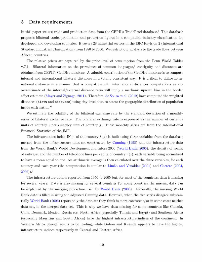
The infrastructure index INi(j) of the country i (j) is built using three variables from the database
merged from the infrastructure data set constructed by Canning (1998) and the infrastructure data
from the World Bank’s World Development Indicators 2006 (World Bank, 2006): the density of roads,
of railways, and the number of telephone lines per capita of country i (j), each variable being normalized
to have a mean equal to one. An arithmetic average is then calculated over the three variables, for each
country and each year (the computation is similar to Limao and Venables (2001) and Carrere (2004,
2006)).7
The infrastructure data is reported from 1950 to 2005 but, for most of the countries, data is missing
for several years. Data is also missing for several countries.For some countries the missing data can
be explained by the merging procedure used by World Bank (2006). Generally, the missing World
Bank data is filled in using the adjusted Canning data. However, when the two series disagree substan-
tially World Bank (2006) report only the data set they think is more consistent, or in some cases neither
data set, in the merged data set. This is why we have data missing for some countries like Canada,
Chile, Denmark, Mexico, Russia etc. North Africa (especially Tunisia and Egypt) and Southern Africa
(especially Mauritius and South Africa) have the highest infrastructure indices of the continent. In
Western Africa Senegal seems to be leading, while Gabon and Rwanda appears to have the highest
infrastructure indices respectively in Central and Eastern Africa.
10
Finally, data on the indicators for high entry barriers in both countries that serve as excluded vari-
ables for the Heckman selection method are obtained from the World Bank’s Doing Business dataset
(http://www.doingbusiness.org/data). Tables 6, 7 and 8 display the descriptive statistics respec-
tively for the whole sample, for the intra-African trade and for SADC. The average bilateral flow for the
whole sample (23,802) five times higher than the corresponding figure for intra-African trade (4,561)
but lower than the average bilateral trade flow within SADC (27,925). The levels of the infrastructure
indices are however in average lower in SADC and in Africa than in the whole sample. We have to
note that the data on infrastructure is reported only for a fraction of the dataset (a little bit less than
3,000,000 observations versus 15,459,569 observations for the bilateral trade flows).
4 Analysis of border effects
This section is divided as follows. We first present a general overview of intra-African border effects, by
estimating different specifications either with or without the infrastructure index. Then, we assess how
these border effects are impacted on by tariffs. Finally, we contrast these results with border effects
arising from trade between European exporters and African exporters. This comparison would help
us to figure out whether Africa is more open to overseas markets than to foreign markets of their own
region.
4.1 Intra-African border effects
4.1.1 Preliminary results
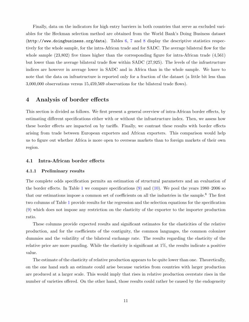
The complete odds specification permits an estimation of structural parameters and an evaluation of
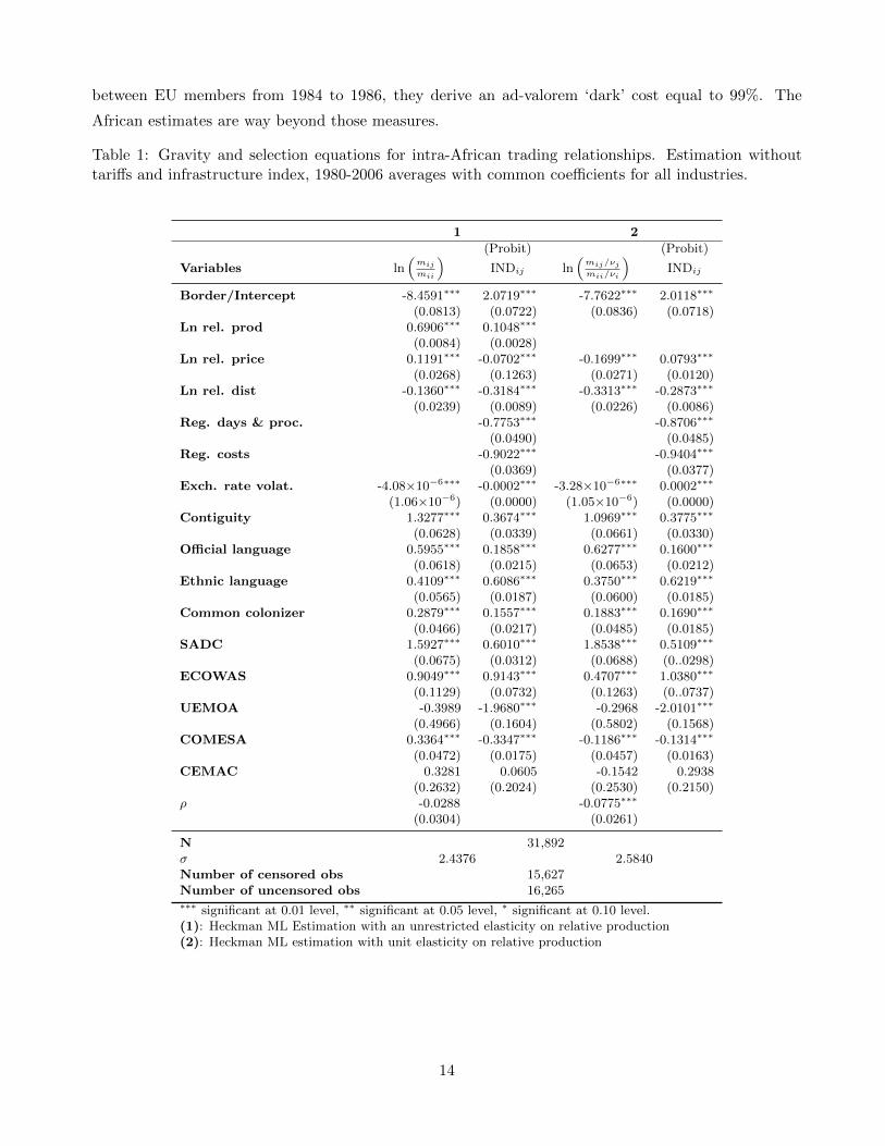
the border effects. In Table 1 we compare specifications (9) and (10). We pool the years 1980–2006 so
that our estimations impose a common set of coefficients on all the industries in the sample.8 The first
two columns of Table 1 provide results for the regression and the selection equations for the specification
(9) which does not impose any restriction on the elasticity of the exporter to the importer production
ratio.
These columns provide expected results and significant estimates for the elasticities of the relative
production, and for the coefficients of the contiguity, the common languages, the common colonizer
dummies and the volatility of the bilateral exchange rate. The results regarding the elasticity of the
relative price are more puzzling. While the elasticity is significant at 1%, the results indicate a positive
value.
The estimate of the elasticity of relative production appears to be quite lower than one. Theoretically,
on the one hand such an estimate could arise because varieties from countries with larger production
are produced at a larger scale. This would imply that rises in relative production overstate rises in the
number of varieties offered. On the other hand, those results could rather be caused by the endogeneity
11
biases mentioned earlier on Head and Mayer (2000). In this regard specification (10), illustrated in the
two last columns of Table 1, presents clear advantages.
Results from these last two columns are broadly similar to the previous results except for the elas-
ticities of the relative distance and of the relative price. The elasticity of the relative distance is higher
than in the previous results. In their meta-analysis Disdier and Head (2008) find an average elasticity
of 0.9. Therefore, while the new result seems to have improved, it is still lower than what is suggested
in the literature. An improvement is also noticed for the relative price elasticity which now becomes
negative as one would have expected. However, the results indicate an unreasonably small value.9 Ac-
tually, this result of low price elasticities when using direct proxies for prices is quite frequent in the
literature (Head and Mayer, 2000; Erkel-Rousse and Mirza, 2002; de Sousa et al., 2012).
The findings suggest therefore that endogeneity biases are quite critical for these two variables.
Since specification (10) is the most appropriate to mitigate endogeneity biases, our further empirical
analysis of border effects will be based on it. The results from these last two columns of Table 1 indicate
that African countries sharing a common border trade 3 (exp(1.0969)) times more than non-contiguous
African countries; those having a common official language trade 1.87 (exp(0.6277)) times more; those
sharing a common ethnic language trade 1.45 (exp(0.3750)); times more, and those who had a common
colonizer trade 1.21 (exp(0.1883)) times more.
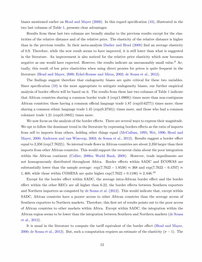
We now focus on the analysis of the border effects. There are several ways to express their magnitude.
We opt to follow the dominant trend in the literature by expressing borders effects as the ratio of imports
from self to imports from others, holding other things equal (McCallum, 1995; Wei, 1996; Head and
Mayer, 2000; Anderson and van Wincoop, 2003; de Sousa et al., 2012). Results suggest a border effect
equal to 2,350 (exp(7.7622)). So internal trade flows in African countries are about 2,350 larger than their
imports from other African countries. This would support the recurrent claim about the poor integration
within the African continent (Collier, 2006a; World Bank, 2008). However, trade impediments are
not homogeneously distributed throughout Africa. Border effects within SADC and ECOWAS are
substantially lower than the sample average: exp(7.7622 − 1.8538) ≈ 368 and exp(7.7622 − 0.4707) ≈1, 468; while those within COMESA are quite higher exp(7.7622 + 0.1186) ≈ 2, 646.10
Except for the border effect within SADC, the average intra-African border effect and the border
effect within the other RECs are all higher than 6.22, the border effects between Southern exporters
and Northern importers as computed by de Sousa et al. (2012). This would indicate that, except within
SADC, African countries have a poorer access to other African countries than the average access of
Southern exporters to Northern markets. Therefore, this first set of results points out to the poor access
of African countries to other markets within Africa. Except within SADC, the integration within the
African region seems to be lower than the integration between Southern and Northern markets (de Sousa
et al., 2012).
It is usual in the literature to compute the tariff equivalent of the border effect (Head and Mayer,
2000; de Sousa et al., 2012). But, such a computation requires an estimate of the elasticity (σ − 1). The
12
coefficient of the relative price would be the designated source for this parameter. The problem is that,
as previously explained, this estimate is quite disappointing, with a value much lower than expected. Yet
the literature provides estimates of the trade elasticity. While Head and Ries (2001), Eaton and Kortum
(2002), and Lai and Trefler (2002) suggest an elasticity around 8 for developed countries in recent years,
the consensus in the literature seems to have shifted towards half of that value (Head and Mayer,
2013b). Using disaggregated price and trade-flow data for 123 countries in the year 2004 Simonovska
and Waugh (2014) also found estimates roughly equal to 4 which implies doubling the welfare gains
from international trade.
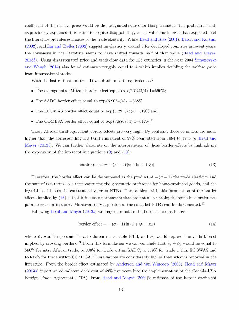
With the last estimate of (σ − 1) we obtain a tariff equivalent of:
• The average intra-African border effect equal exp (7.7622/4)-1=596%;
• The SADC border effect equal to exp (5.9084/4)-1=338%;
• The ECOWAS border effect equal to exp (7.2915/4)-1=519% and;
• The COMESA border effect equal to exp (7.8808/4)-1=617%.11
These African tariff equivalent border effects are very high. By contrast, those estimates are much
higher than the corresponding EU tariff equivalent of 99% computed from 1984 to 1986 by Head and
Mayer (2013b). We can further elaborate on the interpretation of those border effects by highlighting
the expression of the intercept in equations (9) and (10):
border effect = − (σ − 1) [α+ ln (1 + ξ)] (13)
Therefore, the border effect can be decomposed as the product of − (σ − 1) the trade elasticity and
the sum of two terms: α a term capturing the systematic preference for home-produced goods, and the
logarithm of 1 plus the constant ad valorem NTBs. The problem with this formulation of the border
effects implied by (13) is that it includes parameters that are not measurable; the home-bias preference
parameter α for instance. Moreover, only a portion of the so-called NTBs can be documented.12
Following Head and Mayer (2013b) we may reformulate the border effect as follows
border effect = − (σ − 1) ln (1 + ψc + ψd) (14)
where ψc would represent the ad valorem measurable NTB, and ψd would represent any ‘dark’ cost
implied by crossing borders.13 From this formulation we can conclude that ψc + ψd would be equal to
596% for intra-African trade, to 338% for trade within SADC, to 519% for trade within ECOWAS and
to 617% for trade within COMESA. These figures are considerably higher than what is reported in the
literature. From the border effect estimated by Anderson and van Wincoop (2003), Head and Mayer
(2013b) report an ad-valorem dark cost of 49% five years into the implementation of the Canada-USA
Foreign Trade Agreement (FTA). From Head and Mayer (2000)’s estimate of the border coefficient
13
between EU members from 1984 to 1986, they derive an ad-valorem ‘dark’ cost equal to 99%. The
African estimates are way beyond those measures.
Table 1: Gravity and selection equations for intra-African trading relationships. Estimation withouttariffs and infrastructure index, 1980-2006 averages with common coefficients for all industries.
1 2
(Probit) (Probit)
Variables ln(mij
mii
)INDij ln
(mij/νjmii/νi
)INDij
Border/Intercept -8.4591∗∗∗ 2.0719∗∗∗ -7.7622∗∗∗ 2.0118∗∗∗
(0.0813) (0.0722) (0.0836) (0.0718)Ln rel. prod 0.6906∗∗∗ 0.1048∗∗∗
(0.0084) (0.0028)Ln rel. price 0.1191∗∗∗ -0.0702∗∗∗ -0.1699∗∗∗ 0.0793∗∗∗
(0.0268) (0.1263) (0.0271) (0.0120)Ln rel. dist -0.1360∗∗∗ -0.3184∗∗∗ -0.3313∗∗∗ -0.2873∗∗∗
(0.0239) (0.0089) (0.0226) (0.0086)Reg. days & proc. -0.7753∗∗∗ -0.8706∗∗∗
(0.0490) (0.0485)Reg. costs -0.9022∗∗∗ -0.9404∗∗∗
(0.0369) (0.0377)Exch. rate volat. -4.08×10⁻⁶∗∗∗ -0.0002∗∗∗ -3.28×10⁻⁶∗∗∗ 0.0002∗∗∗
(1.06×10⁻⁶) (0.0000) (1.05×10⁻⁶) (0.0000)Contiguity 1.3277∗∗∗ 0.3674∗∗∗ 1.0969∗∗∗ 0.3775∗∗∗
(0.0628) (0.0339) (0.0661) (0.0330)Official language 0.5955∗∗∗ 0.1858∗∗∗ 0.6277∗∗∗ 0.1600∗∗∗
(0.0618) (0.0215) (0.0653) (0.0212)Ethnic language 0.4109∗∗∗ 0.6086∗∗∗ 0.3750∗∗∗ 0.6219∗∗∗
(0.0565) (0.0187) (0.0600) (0.0185)Common colonizer 0.2879∗∗∗ 0.1557∗∗∗ 0.1883∗∗∗ 0.1690∗∗∗
(0.0466) (0.0217) (0.0485) (0.0185)SADC 1.5927∗∗∗ 0.6010∗∗∗ 1.8538∗∗∗ 0.5109∗∗∗
(0.0675) (0.0312) (0.0688) (0..0298)ECOWAS 0.9049∗∗∗ 0.9143∗∗∗ 0.4707∗∗∗ 1.0380∗∗∗
(0.1129) (0.0732) (0.1263) (0..0737)UEMOA -0.3989 -1.9680∗∗∗ -0.2968 -2.0101∗∗∗
(0.4966) (0.1604) (0.5802) (0.1568)COMESA 0.3364∗∗∗ -0.3347∗∗∗ -0.1186∗∗∗ -0.1314∗∗∗
(0.0472) (0.0175) (0.0457) (0.0163)CEMAC 0.3281 0.0605 -0.1542 0.2938
(0.2632) (0.2024) (0.2530) (0.2150)ρ -0.0288 -0.0775∗∗∗
(0.0304) (0.0261)
N 31,892σ 2.4376 2.5840Number of censored obs 15,627Number of uncensored obs 16,265∗∗∗ significant at 0.01 level, ∗∗ significant at 0.05 level, ∗ significant at 0.10 level.(1): Heckman ML Estimation with an unrestricted elasticity on relative production(2): Heckman ML estimation with unit elasticity on relative production
14
4.1.2 Accounting for infrastructure
We may need some less conventional sources of resistance to improve the estimates of the border effects
arising in intra-African trade.14 The usual sources of resistance – cross border tariffs or border compli-
ance costs – are not sufficient to explain the high level of border effects within Africa. Quoting Gross-
man (1998), Head and Mayer (2013b) mention three possible explanations: informational impediments
to trade, localized and historically determined tastes, and business networks. It is quite difficult to get
proxies for these dimensions, especially for intra-African trade. However, by using the infrastructure
indices of the importer and the exporter together, we might get an imperfect but useful proxy of the
business network which might be insightful for explaining the relatively low border resistance prevailing
in SADC.
While one might conjecture that SADC has established more effective institutions to promote re-
gional integration, another plausible explanation may emerge: the high quality of the transport infras-
tructure of several SADC countries (South Africa, Botswana, Namibia) may favor trade flows within
the region. It would be useful to use data on quality of transport-related infrastructure to disentangle
the impact of the infrastructure from the border effects.
The last two columns of Table 2 provide results with the infrastructure index. The first two columns
of the same table serve as a benchmark as they provide estimations with the same sample as with
the last two but without the infrastructure index. With the inclusion of the infrastructure index the
sample size drops significantly from 31,892 to 10,136. This drop of the sample size has an impact on
the elasticity of relative price and on the coefficient of the ethnic language dummy which now become
insignificant. Yet, we obtain a distance elasticity of about -0.8097, which suggests that the inclusion of
the infrastructure indices allow the distance elasticity to increase towards the estimate reported by Dis-
dier and Head (2008). Furthermore, with the infrastructure indices we find that contiguous countries
trade 1.73 (exp(0.5496)) more, countries sharing a common official language trade 2.04 (exp(0.7110))
more, and countries who had a common colonizer trade 1.73 (exp(0.5504)) more.
The impact of the infrastructure indices on the intra-African border effects is even more remarkable.
While the average intra-African border effects arising from the first two columns of Table 2 is about
2,750 (exp(7.9192)), it shrinks to 108 (exp(4.6806)) when the infrastructure indices of the importer and
the exporter are taken into account. Considering the infrastructure index implies a sharp decrease in
the average intra-African border effects. Actually this figure implies that internal trade flows in African
countries are about 108 larger than their imports from other African countries, after controlling for
distances, languages, contiguity effects, common colonizer effects, and infrastructure.
It is even more interesting to assess the border effects within the different regional groupings. With
respectively 22 (exp(4.6806-1.6053)), 33 (exp(4.6806-1.1861)) and 87 (exp(4.6806-0.2111)), the border
effects in SADC and ECOWAS are as before significantly lower than the continental average; while those
of COMESA are only slightly smaller. Therefore, after accounting for bilateral tariffs by deducting the
simple average world tariff (12.5%) the tariff equivalent of the sum of ‘grey’ and ‘dark’ costs becomes:
15
• exp (4.6806/4)-1-0.125=209.5% for intra-African trade;
• exp (3.0753/4)-1-0.125=103.5% for trade within SADC;
• exp (3.4945/4)-1-0.125=127.5% for trade within ECOWAS; and
• exp (4.4695/4)-1-0.125=193.5% for trade within COMESA.
Except for intra-African trade and COMESA, these ‘grey’ and ‘dark’ costs are low comparatively
to the border effects tariff equivalent of 99% for trade within the EU (Head and Mayer, 2013b). With
the inclusion of the infrastructure indices, the measurement of border effects and ‘dark’ costs for SADC
and ECOWAS are more in line with other international estimations. SADC is the only REC that
displays a rising trend for the intraregional trade share in GDP (de Melo and Tsikata, 2014). The
SADC intraregional trade share in GDP is actually on average one of the highest in the region. The
proportion of intraregional rose from 1.4% in 1970 to 12.2% in 2000. Furthermore, while the intra-SADC
trade volume increased by only 26% between 1970 and 1980, it markedly increased by 206% between
1980 and 1985 and 75% between 1990 and 2000 (Babarinde, 2003)1.
ECOWAS is another REC that experiences some success in its integration endeavours. There is evi-
dence of trade creation since the inception of the ECOWAS. Intra-ECOWAS trade volume significantly
increased by 705% between 1970 and 1980 (following the launch of ECOWAS), 122% between 1980 and
1990, and 117% between 1990 and 1998 (Babarinde, 2003).2 Moreover, ECOWAS includes the West
African Economic and Monetary Union (WAEMU) members who share a common currency, and have
achieved deeper integration (de Melo and Tsikata, 2014).
Table 9 in Appendix B reports an estimation including the bilateral tariffs but not the infrastructure
indices. Compared to Table 1, this estimation implies a sharp decrease of the number of observations:
from 31,892 to 5,916. The reason is because data on the bilateral tariffs are available only between 1989
and 2001. This shortfall in the number of observations may be an explanation why, surprisingly, the
inclusion of bilateral tariffs does not seem to improve the results. First, the elasticity of the tariff factor
is only significant at the 10% significance level. But, more important the border effects in the presence
of tariffs, 2,914 (exp(7.9772) cfr. the two last columns of Table 9) are even higher than in their absence
(cfr. Table 1).
1The inauguration of the first post-apartheid government in South Africa (SA) and the accession of SA to the SADCseemed to have contributed substantially to the jump in intraregional trade volume: 303% between 1990 and 1995.
2In 1999 the ECOWAS initiated a traveler’s check program to facilitate trade and the movement of people within theregion. Additional achievements of the ECOWAS comprise a trans-African highway, a trans-African pipeline that suppliesNigeria’s natural gas to some member countries, and the repeal of visa requirements for ECOWAS citizens (Babarinde,2003).
16
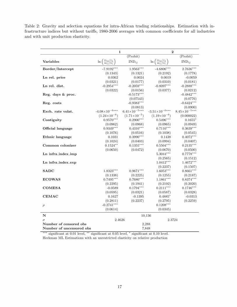
Table 2: Gravity and selection equations for intra-African trading relationships. Estimation with in-frastructure indices but without tariffs, 1980-2006 averages with common coefficients for all industriesand with unit production elasticity.
1 2
(Probit) (Probit)
Variables ln(mij/νjmii/νi
)INDij ln
(mij/νjmii/νi
)INDij
Border/Intercept -7.9192∗∗∗ 1.9563∗∗∗ -4.6806∗∗∗ 2.7636∗∗∗
(0.1343) (0.1321) (0.2192) (0.1778)Ln rel. price 0.0362 0.0024 0.0019 -0.0059
(0.0321) (0.0177) (0.0310) (0.0181)Ln rel. dist. -0.2954∗∗∗ -0.2059∗∗∗ -0.8097∗∗∗ -0.2888∗∗∗
(0.0322) (0.0156) (0.0377) (0.0212)Reg. days & proc. -0.5173∗∗∗ -0.4842∗∗∗
(0.07543) (0.0776)Reg. costs -0.9383∗∗∗ -0.6424∗∗∗
(0.0813) (0.0900)Exch. rate volat. -4.08×10⁻⁶∗∗∗ 6.41×10⁻⁵∗∗∗ -3.51×10⁻⁶∗∗∗ 8.45×10⁻⁵∗∗∗
(1.24×10⁻⁶) (1.71×10⁻⁵) (1.19×10⁻⁶) (0.000022)Contiguity 0.9570∗∗∗ 0.2900∗∗∗ 0.5496∗∗∗ 0.1655∗
(0.0962) (0.0968) (0.0965) (0.0949)Official language 0.9349∗∗∗ 0.4310∗∗∗ 0.7110∗∗∗ 0.3639∗∗∗
(0.1076) (0.0516) (0.1038) (0.0545)Ethnic language 0.1031 0.3990∗∗∗ 0.1438 0.4072∗∗∗
(0.1024) (0.0403) (0.0994) (0.0407)Common colonizer 0.1524∗∗ 0.1355∗∗∗ 0.5504∗∗∗ 0.2135∗∗∗
(0.0650) (0.0472) (0.0670) (0.0500)Ln infra index imp 5.3044∗∗∗ 0.7778∗∗∗
(0.2565) (0.1512)Ln infra index exp 1.0412∗∗∗ 1.4672∗∗∗
(0.2237) (0.1507)SADC 1.8323∗∗∗ 0.9671∗∗∗ 1.6053∗∗∗ 0.8661∗∗∗
(0.1338) (0.2225) (0.1255) (0.2187)ECOWAS 0.7495∗∗∗ 0.7680∗∗∗ 1.1861∗∗∗ 0.8374∗∗∗
(0.2295) (0.1941) (0.2192) (0.2020)COMESA -0.0589 0.1794∗∗∗ 0.2111∗∗∗ 0.1746∗∗∗
(0.0595) (0.0321) (0.0587) (0.0328)CEMAC 0.1627 -0.1395 0.4885∗ -0.0313
(0.2811) (0.2237) (0.2795) (0.2259)ρ -0.2741∗∗∗ 0.1208∗∗∗
(0.0614) (0.0345)
N 10,136σ 2.4626 2.3724Number of censored obs 2,288Number of uncensored obs 7,848∗∗∗ significant at 0.01 level, ∗∗ significant at 0.05 level, ∗ significant at 0.10 level.Heckman ML Estimations with an unrestricted elasticity on relative production
17
4.1.3 The impact of bilateral tariffs
The joint inclusion of bilateral tariffs and infrastructure indices (cfr. Table 10 in Appendix B) does
not bring much of an improvement. This joint inclusion reduces the sample size to 1,616 observations.
While the implied border effects 1,582 (exp(7.3662)), are lower than in Table 9, they are still much
higher than in the results derived from the specification with infrastructure indices but without tariffs
(displayed in Table 2).
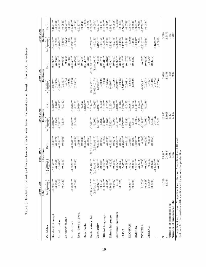
The evolution of the border effects through time is analyzed next. Whether we include infrastructure
indices or not, two opposite outcomes emerge from this analysis. In Table 3 we can see the evolution
of border effects without accounting for infrastructure indices. The first five columns of Table 3 shows
the evolution when tariffs are not accounted for. We can notice there that border effects decreased from
5,041 (exp(8.5254)) between 1980-1988 to 2,243 (exp(7.7156)) between 1989-1997, and finally to 1,458
(exp(7.2846)). For SADC the border effects also decreased 479 (exp(7.7156-1.5445)) between 1989-1997
to 203 (exp(7.2846-1.9727)) between 1998-2006. Regarding ECOWAS, border effects decrease from
2,598 (exp(8.5254-0.6630)) between 1980-1988 to 389 (exp(7.7156-1.7512)) between 1989-1997 but then
increased slightly to 454 (exp(7.2846-1.1671)) between 1998-2006.
When we take tariffs into consideration, as in the last four columns of Table 3, border effects
also diminished from 5,998 (exp(8.6992)) between 1989-1997 to 1,395 (exp(7.2403)) between 1998-2006.
For SADC they also decreased from 469 (exp(8.6992-2.5477)) between 1989-1997 to 166 (exp(7.2403-
2.1271)). Let us now focus on the results with infrastructure indices. In doing so we disregard the
impact of bilateral tariffs. In this configuration, border effects evolve in the opposite direction. Table 4
shows the evolution of border effects when the infrastructure indices are included as regressors. Border
effects rise from 23 (exp(3.1396)) between 1980-1988 to 187 (exp(5.2314)) and to 1,914 (exp(7.5567)).
For SADC border effects increase from 37 (exp(5.2314-1.6227)) between 1989-1997 to 190 (exp(7.5567-
2.3113)) between 1998-2006.
The fact that tables 3 and 4 display evolutions in opposite direction might give ground to the
hypothesis that the decline of border effects is mostly driven by the improvement of transport and
communication infrastructure than by the reduction of NTBs like quotas, export restraints and s forth.
However, more information especially on NTBs is needed to confirm this suggestion.
18
Tab
le3:
Evolu
tion
ofin
tra-
Afr
ican
bor
der
effec
tsov
erti
me.
Est
imat
ion
sw
ithou
tin
frast
ruct
ure
ind
exes
.
1980-1
988
1989-1
997
1998-2
006
1989-1
997
1998-2
006
OL
SH
eckm
an
Heckm
an
Heckm
an
Heckm
an
Varia
ble
sln
( m ij/νj
mii/νi
)ln
( m ij/νj
mii/νi
)IN
Dij
ln( m i
j/νj
mii/νi
)IN
Dij
ln( m i
j/νj
mii/νi
)IN
Dij
ln( m i
j/νj
mii/νi
)IN
Dij
Bord
er/In
tercep
t-8
.5254∗∗∗
-7.7
156∗∗∗
1.7
130∗∗∗
-7.2
846∗∗∗
1.9
672∗∗∗
-8.6
992∗∗∗
2.8
092∗∗∗
-7.2
403∗∗∗
2.1
391∗∗∗
(0.1
349)
(0.1
347)
(0.1
071)
(0.1
533)
(0.1
042)
(0.4
969)
(0.2
608)
(0.3
302)
(0.2
287)
Ln
rel.
pric
e-0
.0461
-0.0
815∗∗
-0.0
554∗∗∗
-1.0
232∗∗∗
0.6
053∗∗
-0.4
984∗∗∗
0.2
128∗∗∗
-0.8
970∗∗∗
0.3
815∗∗∗
(0.0
420)
(0.0
384)
(0.0
161)
(0.1
374)
(0.0
342)
(0.1
361)
(0.0
543)
(0.3
091)
(0.0
845)
Ln
tariff
facto
r-0
.1733
-0.2
148
-1.8
252∗
-0.5
500∗∗∗
(0.5
262)
(0.1
587)
(1.0
206)
(0.2
018)
Ln
rel.
dis
t.-0
.2807∗∗∗
-0.3
020∗∗∗
-0.2
867∗∗∗
-0.4
592∗∗∗
-0.2
578∗∗∗
0.0
238
-0.5
958∗∗∗
-0.4
211∗∗∗
-0.2
446∗∗∗
(0.0
349)
(0.0
386)
(0.0
134)
(0.0
420)
(0.0
153)
(0.1
861)
(0.0
582)
(0.0
819)
(0.0
282)
Reg.
days
&p
roc.
-1.0
938∗∗∗
-0.7
630∗∗∗
-1.3
334∗∗∗
-0.9
127∗∗∗
(0.0
625)
(0.0
821)
(0.1
248)
(0.1
824)
Reg.
cost
s-0
.6330∗∗∗
-1.1
078∗∗∗
-0.6
530∗∗∗
-1.0
886
(0.0
658)
(0.0
493)
(0.1
287)
(0.0
921)
Exch
.rate
vola
t.-2
.38×
10−6∗∗
-7.4
5×
10−5∗
22.2
1×
10−5∗∗∗
-0.0
441∗∗∗
0.0
114∗∗∗
25.1
3×
10−5
-31.2×
10−5∗∗∗
-0.0
766∗∗∗
0.0
309∗∗∗
(1.0
7×
10−6)
(4.0
3×
10−5)
(2.5
5×
10−5)
(0.0
073)
(0.0
027)
(33.6
5×
10−5)
(8.4
8×
10−5)
(0.0
153)
(0.0
074)
Conti
gu
ity
0.9
032∗∗∗
1.3
205∗∗∗
0.6
383∗∗∗
1.3
752∗∗∗
0.1
917∗∗∗
1.9
645∗∗∗
0.0
386
1.1
004∗∗∗
0.4
117∗∗∗
(0.1
156)
(0.0
988)
(0.0
556)
(0.1
617)
(0.0
526)
(0.3
050)
(0.1
474)
(0.3
151)
(0.1
125)
Offi
cia
lla
ngu
age
0.6
003∗∗∗
0.6
212∗∗∗
0.0
252
0.4
110∗∗∗
0.3
132∗∗∗
0.1
988
-0.2
061∗∗∗
0.6
475∗∗∗
0.3
136∗∗∗
(0.1
685)
(0.0
969)
(0.0
336)
(0.1
042)
(0.0
297)
(0.2
086)
(0.0
704)
(0.2
269)
(0.0
635)
Eth
nic
lan
gu
age
0.7
666∗∗∗
0.1
232
0.7
326∗∗∗
0.7
322∗∗∗
0.3
125∗∗∗
0.4
707∗∗
0.7
294∗∗∗
0.7
383∗∗∗
0.3
821∗∗∗
(0.1
402)
(0.0
949)
(0.0
278)
(0.0
994)
(0.0
285)
(0.2
146)
(0.0
640)
(0.2
176)
(0.0
618)
Com
mon
colo
niz
er
0.0
105
0.2
677∗∗∗
0.2
889∗∗∗
0.6
177∗∗∗
-0.1
246∗∗∗
0.8
680∗∗∗
0.3
902∗∗∗
0.5
838∗∗∗
-0.0
372
(0.0
925)
(0.0
749)
(0.0
353)
(0.0
943)
(0.0
314)
(0.1
988)
(0.0
827)
(0.1
822)
(0.0
613)
SA
DC
1.5
445∗∗∗
0.4
002∗∗∗
1.9
727∗∗∗
0.9
220∗∗∗
2.5
477∗∗∗
0.5
416∗∗∗
2.1
271∗∗∗
0.5
613∗∗∗
(0.0
890)
(0.0
419)
(0.1
313)
(0.0
475)
(0.3
011)
(0.1
276)
(0.2
448)
(0.0
761)
EC
OW
AS
0.6
630∗∗∗
1.7
512∗∗∗
0.2
818∗∗
1.1
671∗∗∗
0.9
696∗∗∗
1.8
858
-0.7
046∗
1.5
618
1.0
870∗∗∗
(0.1
395)
(0.3
946)
(0.1
299)
(0.4
455)
(0.1
702)
(1.6
900)
(0.4
022)
(1.1
523)
(0.3
836)
UM
EO
A-2
.3719∗∗∗
-1.2
296∗∗∗
-1.3
904
-1.4
117∗∗∗
-3.6
930∗∗
-1.5
325∗∗∗
(0.5
417)
(0.2
727)
(0.8
952)
(0.2
401)
(1.5
588)
(0.5
606)
CO
ME
SA
0.1
531∗
-0.0
793
0.0
003
-0.1
962∗∗
-0.2
766∗∗∗
-0.5
044∗∗
-0.0
070
-0.9
261∗∗∗
-0.2
776∗∗∗
(0.0
848)
(0.0
700)
(0.0
254)
(0.0
983)
(0.0
289)
(0.2
207)
(0.0
738)
(0.2
021)
(0.0
584)
CE
MA
C0.5
988∗
-0.2
757
-0.2
318
0.9
629
-0.4
527
-0.6
176∗
(0.3
499)
(0.3
733)
(0.2
555)
(0.6
444)
(0.6
112)
(0.3
212)
ρ-0
.1484∗∗∗
-0.0
120
-0.0
764
0.1
679∗∗∗
(0.0
399)
(0.0
401)
(0.0
766)
(0.0
810)
N4,2
19
13,8
67
13,8
22
2,6
98
3,2
18
σ2.4
344
2.4
883
2.7
058
2.5
398
2.6
479
Nu
mb
er
of
cen
sored
ob
s7,3
00
8,3
27
1,4
42
1,8
71
Nu
mb
er
of
uncenso
red
ob
s6,5
67
5,4
95
1,2
56
1,3
47
∗∗∗
sign
ifica
nt
at
0.0
1le
vel
,∗∗
sign
ifica
nt
at
0.0
5le
vel
,∗
sign
ifica
nt
at
0.1
0le
vel
.H
eckm
an
ML
Est
imati
on
sw
ith
au
nit
elast
icit
yon
rela
tive
pro
du
ctio
n
19
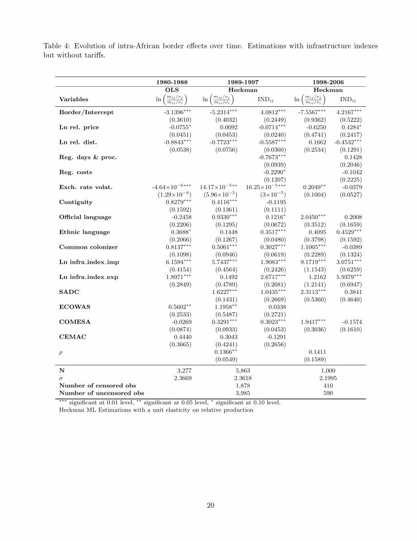
Table 4: Evolution of intra-African border effects over time. Estimations with infrastructure indexesbut without tariffs.
1980-1988 1989-1997 1998-2006
OLS Heckman Heckman
Variables ln(mij/νjmii/νi
)ln
(mij/νjmii/νi
)INDij ln
(mij/νjmii/νi
)INDij
Border/Intercept -3.1396∗∗∗ -5.2314∗∗∗ 4.0812∗∗∗ -7.5567∗∗∗ 4.2167∗∗∗
(0.3610) (0.4032) (0.2449) (0.9362) (0.5222)Ln rel. price -0.0755∗ 0.0092 -0.0714∗∗∗ -0.6250 0.4284∗
(0.0451) (0.0453) (0.0240) (0.4741) (0.2417)Ln rel. dist. -0.8843∗∗∗ -0.7723∗∗∗ -0.5587∗∗∗ 0.1662 -0.4532∗∗∗
(0.0538) (0.0756) (0.0360) (0.2534) (0.1291)Reg. days & proc. -0.7673∗∗∗ 0.1428
(0.0939) (0.2046)Reg. costs -0.2290∗ -0.1042
(0.1207) (0.2225)Exch. rate volat. -4.64×10⁻⁶∗∗∗ 14.17×10⁻⁵∗∗ 16.25×10⁻⁵∗∗∗ 0.2049∗∗ -0.0379
(1.29×10⁻⁶) (5.96×10⁻⁵) (3×10⁻⁵) (0.1004) (0.0527)Contiguity 0.8279∗∗∗ 0.4116∗∗∗ -0.1195
(0.1592) (0.1361) (0.1111)Official language -0.2458 0.9330∗∗∗ 0.1216∗ 2.0450∗∗∗ 0.2008
(0.2206) (0.1295) (0.0672) (0.3512) (0.1659)Ethnic language 0.3688∗ 0.1448 0.3517∗∗∗ 0.4095 0.4529∗∗∗
(0.2066) (0.1267) (0.0480) (0.3798) (0.1592)Common colonizer 0.8137∗∗∗ 0.5061∗∗∗ 0.3027∗∗∗ 1.1005∗∗∗ -0.0389
(0.1098) (0.0946) (0.0619) (0.2289) (0.1324)Ln infra index imp 6.1594∗∗∗ 5.7437∗∗∗ 1.9083∗∗∗ 9.1719∗∗∗ 3.0751∗∗∗
(0.4154) (0.4564) (0.2426) (1.1543) (0.6259)Ln infra index exp 1.8971∗∗∗ 0.1492 2.6717∗∗∗ 1.2162 5.9379∗∗∗
(0.2849) (0.4789) (0.2681) (1.2141) (0.6947)SADC 1.6227∗∗∗ 1.0435∗∗∗ 2.3113∗∗∗ 0.3841
(0.1431) (0.2669) (0.5360) (0.4640)ECOWAS 0.5602∗∗ 1.1958∗∗ 0.0338
(0.2533) (0.5487) (0.2721)COMESA -0.0269 0.3291∗∗∗ 0.3023∗∗∗ 1.9417∗∗∗ -0.1574
(0.0874) (0.0933) (0.0453) (0.3036) (0.1610)CEMAC 0.4440 0.3043 -0.1291
(0.3665) (0.4241) (0.2656)ρ 0.1366∗∗ 0.1411
(0.0549) (0.1589)
N 3,277 5,863 1,000σ 2.3669 2.3618 2.1995Number of censored obs 1,878 410Number of uncensored obs 3,985 590∗∗∗ significant at 0.01 level, ∗∗ significant at 0.05 level, ∗ significant at 0.10 level.Heckman ML Estimations with a unit elasticity on relative production
20
4.2 Intra-African border effects vs Europe-Africa border effects
Table 5 provides results of the estimation of the specification (10) for exports from Europe to Africa. The
first two columns report results without the infrastructure indices, while the last two columns display
results accounting for them. Before commenting on the border effects that apply to European exports
in Africa, let us discuss some of the other results. Few of them are actually noteworthy: countries
previously involved in a colonial relationship and those sharing a language spoken by at least 5% of the
population trade 3 (respectively exp(1.1116) and exp(1.0935)) times more than the sample average.
Surprisingly, memberships to free trade agreements linking African to European countries do not
seem to pay off. The coefficient of the dummy for the European Free Trade Association (EFTA)15 - the
Morocco free trade agreement - is not significant in any of the specifications of Table 5. The results for
Africa Caribbean Pacific (ACP)16 - European Union (EU) preferential trade agreement are even more
surprising: the dummy coefficient is negative. This is quite counter-intuitive as one would expect that
such a preferential trade agreement would boost trade rather than impede it.
According to the last two columns of Table 5 (with infrastructure indices), border effects faced by
European exporters in African countries can be estimated to be about 34 (exp(3.5130)). They are higher
than the average intra-African border effects (108) but lower than the SADC and the ECOWAS border
effects. Hence, while on average African countries seem more open to overseas trade flows than to those
coming from their regional partners, regional economic groupings like SADC and ECOWAS seem to be
more open to their intra-regional trade flows than to European exports. This finding is consistent with
earlier findings showing that, after accounting for the impact of infrastructure, SADC and ECOWAS
border effects get closer to international estimations.
21
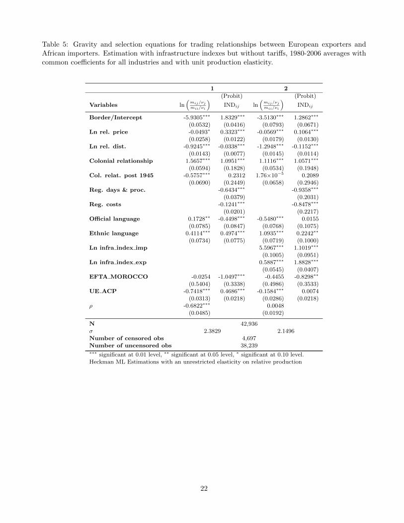
Table 5: Gravity and selection equations for trading relationships between European exporters andAfrican importers. Estimation with infrastructure indexes but without tariffs, 1980-2006 averages withcommon coefficients for all industries and with unit production elasticity.
1 2
(Probit) (Probit)
Variables ln(mij/νjmii/νi
)INDij ln
(mij/νjmii/νi
)INDij
Border/Intercept -5.9305∗∗∗ 1.8329∗∗∗ -3.5130∗∗∗ 1.2862∗∗∗
(0.0532) (0.0416) (0.0793) (0.0671)Ln rel. price -0.0493∗ 0.3323∗∗∗ -0.0569∗∗∗ 0.1064∗∗∗
(0.0258) (0.0122) (0.0179) (0.0130)Ln rel. dist. -0.9245∗∗∗ -0.0338∗∗∗ -1.2948∗∗∗ -0.1152∗∗∗
(0.0143) (0.0077) (0.0145) (0.0114)Colonial relationship 1.5657∗∗∗ 1.0951∗∗∗ 1.1116∗∗∗ 1.0571∗∗∗
(0.0594) (0.1828) (0.0534) (0.1948)Col. relat. post 1945 -0.5757∗∗∗ 0.2312 1.76×10⁻⁵ 0.2089
(0.0690) (0.2449) (0.0658) (0.2946)Reg. days & proc. -0.6434∗∗∗ -0.9358∗∗∗
(0.0379) (0.2031)Reg. costs -0.1241∗∗∗ -0.8478∗∗∗
(0.0201) (0.2217)Official language 0.1728∗∗ -0.4498∗∗∗ -0.5480∗∗∗ 0.0155
(0.0785) (0.0847) (0.0768) (0.1075)Ethnic language 0.4114∗∗∗ 0.4974∗∗∗ 1.0935∗∗∗ 0.2242∗∗
(0.0734) (0.0775) (0.0719) (0.1000)Ln infra index imp 5.5967∗∗∗ 1.1019∗∗∗
(0.1005) (0.0951)Ln infra index exp 0.5887∗∗∗ 1.8828∗∗∗
(0.0545) (0.0407)EFTA MOROCCO -0.0254 -1.0497∗∗∗ -0.4455 -0.8298∗∗
(0.5404) (0.3338) (0.4986) (0.3533)UE ACP -0.7418∗∗∗ 0.4686∗∗∗ -0.1584∗∗∗ 0.0074
(0.0313) (0.0218) (0.0286) (0.0218)ρ -0.6822∗∗∗ 0.0048
(0.0485) (0.0192)
N 42,936σ 2.3829 2.1496Number of censored obs 4,697Number of uncensored obs 38,239∗∗∗ significant at 0.01 level, ∗∗ significant at 0.05 level, ∗ significant at 0.10 level.Heckman ML Estimations with an unrestricted elasticity on relative production
22
5 Conclusion
The results show that on average the African continent is poorly integrated and more open to overseas
export than to intra-African trade flows. However, this negative picture is contrasted by the fact that
two African RECs, SADC and ECOWAS have border effects that are more in line with international
estimations. Hence, there is evidence that these two African RECs are effective in promoting intrare-
gional trade. RECs are expected to increase trade between their members via three channels. The
first is a reduction in tariffs between members; the second is a reduction in NTBs; the third is via the
two components of ‘trade facilitation’: a ‘hard’ component related to tangible transport and telecom-
munications infrastructure; and a ‘soft’ component related to transparency, the business environment,
customs management, and other intangible institutional aspects that may facilitate trading (de Melo
and Tsikata, 2014).
The first two channels are the outcomes of measures that are easier to implement and have generally
been undertaken even by the African RECs that only manage to achieve ‘shallow’ integration (de Melo
and Tsikata, 2014). However, the measures implied by the two components of ‘trade facilitation’ are
much more difficult to put in place. This is especially true for the infrastructure dimension. Our model
explicitly account for that ‘hard’ component. Considering infrastructure indices is an interesting way
to capture the effect of distribution networks which represent, along with imperfect information and
localized tastes, sources of resistance that are generally omitted and can possibly explain the counter-
intuitive high border effects (Head and Mayer, 2013b).
The elasticity of the infrastructure indices are high and significant, suggesting that improving trans-
port and telecommunications infrastructures will go a long way in promoting inter-African trade. So
far only Northern and Southern Africa are well endowed in this regard, and it is clear that building and
improving infrastructure in other parts of the continent will generate additional trade opportunities.
The ‘soft’ component of trade facilitation is likely to be the factor explaining the discrepancies between
the different African RECs in terms of border effects. In this regard SADC and ECOWAS seem to have
set institutions that are more effective in achieving trade integration and allow them to be one step
ahead comparatively to other African RECs.
Yet, even these two RECs are still behind Regional Trade Agreements (RTA) in other continents
in terms of the importance of intra-regional trade share in GDP. While the SADC intra-regional trade
share in GDP – on average one of the highest in the continent – rose from 6% to 11% from 1992 to 2013,
the share of intra-RTA trade worldwide, excluding the EU, increased from 18% in 1990 to 34% in 2008
(from 28% to 51% if EU included). So there is still room for improvement in African RECs regarding
this ‘soft’ component of trade facilitation. Actually, regional integration in Africa was based on the
‘linear model’ of integration, with a stepwise integration of goods, labour, and capital markets, as well
as eventual monetary and fiscal integration. Most of African countries overlooked the importance of
tackling ‘behind-the-border’ impediments to trade, yet this is crucial in global environment characterized
23
by the reduction in trade costs and the subsequent fragmentation of production (de Melo and Tsikata,
2014).
Based on our results, two propositions may help reduce border effects and increase inter-regional
trade in Africa. First is the development of large pan-African infrastructure projects which can con-
tribute to defragmenting Africa by decreasing transport costs. Second is the implementation of the
African free trade zone that might bring free trade among the members by: removing tariffs and NTBs
and implementing trade facilitation, by applying the subsidiarity principle to infrastructure to enhance
the transport network, and by fostering industrial development (de Melo and Tsikata, 2014). These
measures will allow African countries to achieve a ‘deep’ rather than a ‘shallow integration’.
Finally, we have to acknowledge the limitations of the study. The main challenges are the quality and
the availability of the African data. Ideally, anyone would have opted for a more direct way to capture
the impact of distribution networks. Combes et al. (2005) for instance examine the impact of business
and social networks on trade between French regions by using the financial structure and location of
French firms as well as the bilateral stocks of migrants. Moreover, Combes et al. (2005) also use data on
transport costs which allow them to separate the effects of transport infrastructure and administrative
border effects.
Another issue that we are facing is that we rely on data on trade flows between different countries.
This implies that in order to estimate border effects we cannot use LSDV estimation; we rely instead on
the complete odds specification which requires a measure of the trade of a country with itself (“trade
with self”). Generally, this “trade with self” is proxied by using production minus total exports. While,
the complete odds specification has been used by several papers (Head and Mayer, 2000; de Sousa et al.,
2012), the measure of “trade with self” may cause some measurement errors as the procedure may
generate some negative observations for some countries (Head and Mayer, 2013a). The ideal would be
to use databases on commodity flows like in Wolf (2000), Anderson and van Wincoop (2003), Hillberry
and Hummels (2003), and Combes et al. (2005) which include inter- and intraregional trade flows.
However, it can be argued that this kind of datasets represents the exception rather than the norm.
Moreover, in the current state of the data collection on African countries, it will be challenging to get
reliable data on the missing sources of resistance. Getting such data is yet the price to pay to improve
on the analysis of border effects in intra-African trade.
Acknowledgements. Alain Pholo Bala gratefully acknowledges financial support from Economic
Research Southern Africa (ersa), South Africa. The views expressed in this paper and any remaining
errors are ours.
Notes
1With data on inter-provincial trade flows, one can estimate the border effects with a fixed effects specification (Feenstra,
2004).
24
2 Head and Mayer (2013a) offers a more in-depth discussion of those models.3These results might be explained by the fact that in specifications (9) and (10), we are dealing with ratios of trade
flow from j to i to trade flow of i from “self” rather than trade flows per se.4Available through the following download page: http://
www.cepii.fr/anglaisgraph/bdd/TradeProd.htm. In this webpage it is recommended to cite de Sousa et al. (2012)’
reference as the source of the data.5One of the file of the GeoDist database, the dist cepii dataset contains 2 variables indicating whether two countries,
origin and destination, share a common official language, or a common ethnic language, i.e. a language that is spoken by
at least 9% of the population in both countries.6Details on the formulas of distw and distwces are given in Mayer and Zignago (2011, p. 11).7Infrastructure data may be found at the following link:
http://thedata.harvard.edu/dvn/dv/pep/faces/study/StudyPage.xhtml?globalId=hdl:1902.1/11953.8It would have been useful to estimate the gravity model separately for different industries as in Head and Mayer (2000)
and de Sousa et al. (2012), but then we would have ended up with small numbers of observations for some industries.9Head and Mayer (2000) suggest that those low estimates are due to the unobserved variation in relative product quality
which is correlated with relative product price.10Border effects within other African RECs are not statistically different from the sample average.11While for the second estimate, we would obtain a tariff equivalent respectively equal to exp (7.7622/8)-1=164% for
intra-African trade, exp (5.9084/8)-1=109% for SADC, exp (7.2915/8)-1=149% for ECOWAS andexp (7.8808/8)-1=168%
for COMESA. With the same value of the elasticity of trade with respect to trade costs, de Sousa et al. (2012) found a
tariff equivalent of 118% between Southern exporters and Northern importers. Not surprisingly this finding confirms the
previous finding that SADC is the only REC within Africa, where members have easier access to the markets of their
partners than to overseas markets.12While NTBs like quotas, voluntary export restraints and non-automatic import authorizations often have much more
significant effects, only a few databases provide information on non-tariff barriers (e.g. the Doing Business database, the
Trade Facilitation Database, the Logistic Performance Index, the UNCTAD/TRAINS NTM and the CEPII NTM-MAP
databases). The cause of the rarity of databases on NTBs is largely due to the difficulty in collecting the data and in
assembling a consistent cross-country dataset. Unlike tariffs, NTB data are not merely numbers; the relevant information
is often hidden in legal and regulatory documents. Furthermore, these documents are generally not centralized but often
reside in different regulatory agencies. All these issues make the collection of NTB data a very resource-intensive task.
The CEPII NTM-MAP database has been designed to address the shortcomings of the previous databases, yet its index
is only provided for 63 countries for one year over the period 2010-2012 at the country level and two different product
disaggregation levels. Moreover, only 15 African countries are included in the database (Gourdon, 2014).13The concept of ‘dark’ costs results from an analogy with the cosmology concept of dark energy or dark matter. Neither
dark energy nor dark matter can be observed directly, but their presence is inferred to be tremendous. Therefore, ‘dark’
costs represent unobserved or difficult-to-observe trade costs which imply a significant resistance to trade flows. More
information about the astrophysics analogy between ‘dark’ cost and dark energy or dark matter is available in Head and
Mayer (2013b).14The ‘dark’ costs computed by Head and Mayer (2013b) include everything other than tariffs. So they may capture
border compliance costs which may be evaluated (the so-called ‘grey’ costs ψc). Head and Mayer (2013b) acknowledge
that their presentation of the concept of dark costs missed that distinction. However, since they report custom clearance
costs which seem to be negligible (1.8% for EU, and 2.0%-3.4% for the Canada-USA frontier), the ‘dark’ costs seem to be
dominant. Eventually, while the specifications (9) and (10) account for bilateral tariffs, Table 1 does not. So we may still
need to deduct the bilateral tariffs from the estimated ‘dark’ costs. If we use the simple average world tariff (12.5%) as an
approximation (Head and Mayer, 2013b), the intra-African trade dark costs are only slightly affected.15The EFTA is an intergovernmental organization set up for the promotion of free trade and economic integration to
25
the benefit of its four Member States: Iceland, Liechtenstein, Norway, Switzerland (http://www.efta.int).16“The African, Caribbean and Pacific Group of States (ACP) is an organization created by the Georgetown Agree-
ment in 1975. It is composed of 79 African, Caribbean and Pacific states, with all of them, save Cuba, signatories
to the Cotonou Agreement, also known as the “ACP-EC Partnership Agreement” which binds them to the European
Union”(http://www.acp.int/content/secretariat-acp).
References
Ancharaz, V., Mbekeani, K. and Brixiova, Z. (2011), ‘Impediments to Regional Trade Integration in
Africa’, Africa Economic Brief 2(11).
Anderson, J. E. and van Wincoop, E. (2003), ‘Gravity with Gravitas: A Solution to the Border Puzzle’,
American Economic Review 93(1), 170–192.
Artadi, E. V. and Sala-i Martin, X. (2003), The Economic Tragedy of the XXth Century: Growth in
Africa, NBER Working Papers 9865, National Bureau of Economic Research, Inc.
Au, C.-C. and Henderson, J. V. (2006), ‘Are Chinese Cities Too Small?’, Review of Economic Studies
73(3), 549–576.
Babarinde, F. (2003), Regionalism and economic development, in E. U. Nnadozie, ed., ‘African economic
development’, Amsterdam : London : Academic, book; book/illustrated 19, pp. 473–497.
Baldwin, R. and Harrigan, J. (2011), ‘Zeros, Quality, and Space: Trade Theory and Trade Evidence’,
American Economic Journal: Microeconomics 3(2), 60–88.
Behrens, K., Ertur, C. and Koch, W. (2012), ‘Dual Gravity: Using Spatial Econometrics To Control
For Multilateral Resistance’, Journal of Applied Econometrics 27(5), 773–794.
Canning, D. (1998), ‘A database of world stocks of infrastructure, 195095’, The World Bank Economic
Review 12(3), 529–547.
Carrere, C. (2004), ‘African regional agreements: Impact on trade with or without currency unions’,
Journal of African Economies 13(2), 199–239.
Carrere, C. (2006), ‘Revisiting the effects of regional trade agreements on trade flows with proper
specification of the gravity model’, European Economic Review 50(2), 223–247.
Cinyabuguma, M. M. and Putterman, L. (2011), ‘Sub-Saharan Growth Surprises: Being Heterogeneous,
Inland and Close to the Equator Does not Slow Growth Within Africa-super- ’, Journal of African
Economies 20(2), 217–262.
Collier, P. (2006a), ‘Africa : geography and growth’, Proceedings - Economic Policy Symposium -
Jackson Hole pp. 235–252.
26
Collier, P. (2006b), ‘African Growth: Why a ‘Big Push’?’, Journal of African Economies 15(2), 188–211.
Combes, P.-P., Lafourcade, M. and Mayer, T. (2005), ‘The trade-creating effects of business and social
networks: evidence from france’, Journal of International Economics 66(1), 1 – 29.
de Melo, J. and Tsikata, Y. (2014), Regional integration in Africa: Challenges and prospects, Working
Papers P93, FERDI.
de Sousa, J., Mayer, T. and Zignago, S. (2012), ‘Market access in global and regional trade’, Regional
Science and Urban Economics 42(6), 1037–1052.
Disdier, A.-C. and Head, K. (2008), ‘The Puzzling Persistence of the Distance Effect on Bilateral Trade’,
The Review of Economics and Statistics 90(1), 37–48.
Dollar, D. and Easterly, W. (1999), ‘The Search for the Key: Aid, Investment and Policies in Africa’,
Journal of African Economies 8(4), 546–77.
Easterly, W. (2009a), ‘Can the West Save Africa?’, Journal of Economic Literature 47(2), 373–447.
Easterly, W. (2009b), ‘How the Millennium Development Goals are Unfair to Africa’, World Development
37(1), 26–35.
Easterly, W. and Levine, R. (1997), ‘Africa’s Growth Tragedy: Policies and Ethnic Divisions’, The
Quarterly Journal of Economics 112(4), 1203–50.
Eaton, J. and Kortum, S. (2001), ‘Trade in capital goods’, European Economic Review 45(7), 1195–1235.
Eaton, J. and Kortum, S. (2002), ‘Technology, Geography, and Trade’, Econometrica 70(5), 1741–1779.
Eaton, J., Kortum, S. S. and Sotelo, S. (2012), International Trade: Linking Micro and Macro, NBER
Working Papers 17864, National Bureau of Economic Research, Inc.
Eaton, J. and Tamura, A. (1994), ‘Bilateralism and Regionalism in Japanese and U.S. Trade and Direct
Foreign Investment Patterns’, Journal of the Japanese and International Economies 8(4), 478–510.
Economic Commission for Africa (2011), “Boosting Intra-African Trade”. Preparations for the 7th AU
Trade Ministers Conference and the 18th Ordinary Session of the AU Assembly of Heads of State and
Government, Issues paper, Economic Commission for Africa.
Erkel-Rousse, H. and Mirza, D. (2002), ‘Import price elasticities: reconsidering the evidence’, Canadian
Journal of Economics/Revue canadienne d’economique 35(2), 282–306.
Evans, C. L. (2003), ‘The Economic Significance of National Border Effects’, American Economic Review
93(4), 1291–1312.
27
Feenstra, R. C. (2004), Advanced international trade: theory and evidence, Princeton University Press.
Freire, M. E. M., Lall, S. and Leipziger, D. (2015), Africa’s urbanization: Challenges and opportunities,
in C. Monga and J. Y. Lin, eds, ‘The Oxford Handbook of Africa and Economics’, Vol. 1: Context
and Concepts, Oxford University Press, chapter 31, pp. 584–602.
Gourdon, J. (2014), CEPII NTM-MAP: A Tool for Assessing the Economic Impact of Non-Tariff Mea-
sures, Working Papers 2014-24, CEPII research center.
Grossman, G. M. (1998), Comment on: Determinants of Bilateral Trade: Does Gravity Work in a
Neoclassical World?, in J. A. Frankel, ed., ‘The Regionalization of the World Economy’, University
of Chicago Press, pp. 29–31.
Harrigan, J. (1996), ‘Openness to trade in manufactures in the OECD’, Journal of International Eco-
nomics 40(1-2), 23–39.
Head, K. and Mayer, T. (2000), ‘Non-Europe: The magnitude and causes of market fragmentation in
the EU’, Review of World Economics (Weltwirtschaftliches Archiv) 136(2), 284–314.
Head, K. and Mayer, T. (2013a), Gravity Equations: Workhorse,Toolkit, and Cookbook, Working
Papers 2013-27, CEPII research center.
Head, K. and Mayer, T. (2013b), ‘What separates us? sources of resistance to globalization’, Canadian
Journal of Economics/Revue canadienne d’conomique 46(4), 1196–1231.
Head, K. and Ries, J. (2001), ‘Increasing returns versus national product differentiation as an explana-
tion for the pattern of u.s.-canada trade’, American Economic Review 91(4), 858–876.
Helliwell, J. F. (1996), ‘Do National Borders Matter for Quebec’s Trade?’, Canadian Journal of Eco-
nomics 29(3), 507–22.
Helpman, E., Melitz, M. and Rubinstein, Y. (2008), ‘Estimating trade flows: Trading partners and
trading volumes’, The Quarterly Journal of Economics 123(2), 441–487.
Hillberry, R. (1998), ‘Regional trade and the medicine line: The national border effect in u.s. commodity
flow data’, Journal of Borderlands Studies 13(2), 1–17.
Hillberry, R. and Hummels, D. (2003), ‘Intranational Home Bias: Some Explanations’, The Review of
Economics and Statistics 85(4), 1089–1092.
Hummels, D. (1999), Toward a Geography of Trade Costs, GTAP Working Papers 1162, Center for
Global Trade Analysis, Department of Agricultural Economics, Purdue University.
ITC (2012), Africa’s Trade Potential: Export Opportunities in Growth Markets, International Trade
Centre (ITC).
28
Jones, B. (2002), ‘Economic integration and convergence of per capita income in west africa’, African
Development Review 14(1), 18–47.
Krugman, P. (1980), ‘Scale Economies, Product Differentiation, and the Pattern of Trade’, American
Economic Review 70(5), 950–59.
Lai, H. and Trefler, D. (2002), The Gains from Trade with Monopolistic Competition: Specification, Es-
timation, and Mis-Specification, NBER Working Papers 9169, National Bureau of Economic Research,
Inc.
Limao, N. and Venables, A. J. (2001), ‘Infrastructure, geographical disadvantage, transport costs, and
trade’, The World Bank Economic Review 15(3), 451–479.
Mayer, T. and Zignago, S. (2011), Notes on CEPIIs distances measures: The GeoDist database, Working
Papers 2011-25, CEPII research center.
McCallum, J. (1995), ‘National Borders Matter: Canada-U.S. Regional Trade Patterns’, American
Economic Review 85(3), 615–23.
Page, J. (2008), Rowing Against the Current: The Diversification Challenge in Africa’s Resource-Rich
Economies, Brookings Global Economy & Development Working Papers No. 28 December 2008.
Pinkovskiy, M. and Sala-i Martin, X. (2014), ‘Africa is on time’, Journal of Economic Growth 19(3), 311–
338.
Redding, S. and Venables, A. J. (2004), ‘Economic geography and international inequality’, Journal of
International Economics 62(1), 53–82.
Sachs, J. D. and Warner, A. M. (1997), ‘Sources of Slow Growth in African Economies’, Journal of
African Economies 6(3), 335–76.
Simonovska, I. and Waugh, M. E. (2014), ‘The elasticity of trade: Estimates and evidence’, Journal of
International Economics 92(1), 34 – 50.
UNECA (2010), Assessing Regional Integration in Africa IV: Enhancing Intra-African Trade, United
Nations Economic Commission for Africa.
Wei, S.-J. (1996), Intra-National versus International Trade: How Stubborn are Nations in Global
Integration?, NBER Working Papers 5531, National Bureau of Economic Research, Inc.
Wolf, H. C. (2000), ‘Intranational home bias in trade’, The Review of Economics and Statistics
82(4), 555–563.
World Bank (2006), World Development Indicators 2006, number 8151 in ‘World Bank Publications’,
The World Bank.
29

World Bank (2008), World Development Report 2009: Reshaping Economic Geography, World Bank.
30
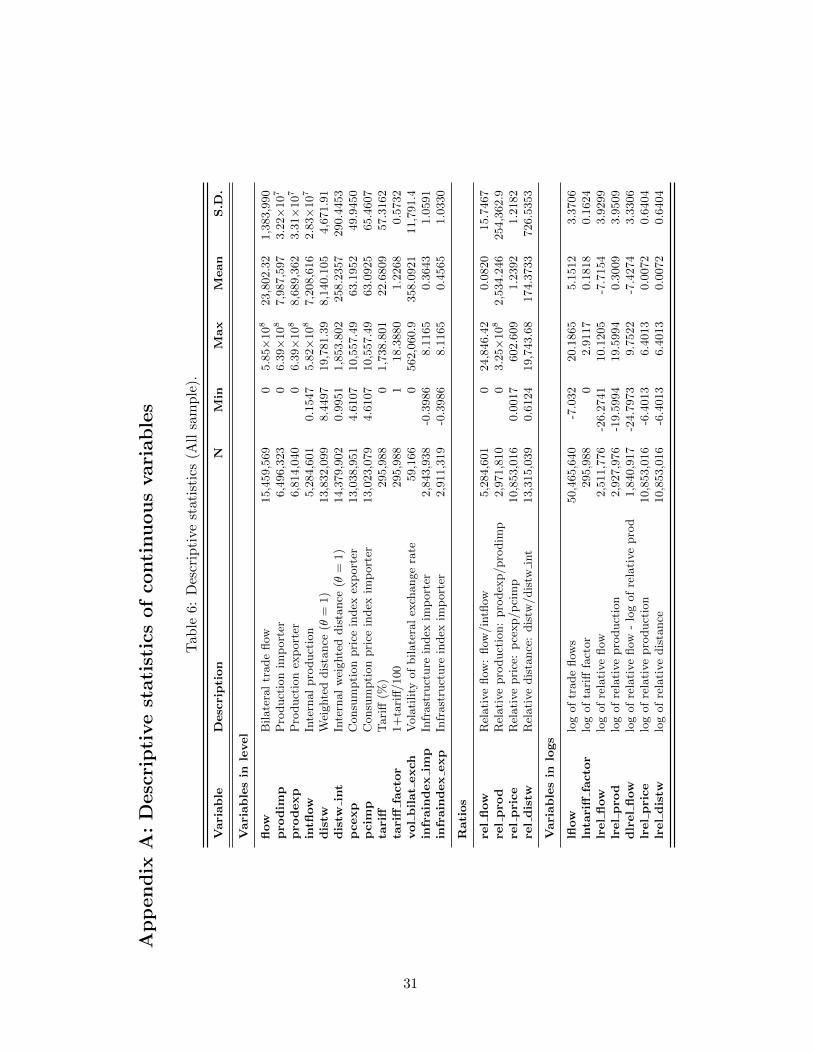
Ap
pen
dix
A:
Desc
rip
tive
stati
stic
sof
conti
nu
ou
svari
ab
les
Tab
le6:
Des
crip
tive
stat
isti
cs(A
llsa
mp
le).
Vari
able
Desc
ripti
on
NM
inM
ax
Mean
S.D
.
Vari
able
sin
level
flow
Bilate
ral
trade
flow
15,4
59,5
69
05.8
5×
108
23,8
02.3
21,3
83,9
90
pro
dim
pP
roduct
ion
imp
ort
er6,4
96,3
23
06.3
9×
108
7,9
87,5
97
3.2
2×
107
pro
dexp
Pro
duct
ion
exp
ort
er6,8
14,0
40
06.3
9×
108
8,6
89,3
62
3.3
1×
107
intfl
ow
Inte
rnal
pro
duct
ion
5,2
84,6
01
0.1
547
5.8
2×
108
7,2
08,6
16
2.8
3×
107
dis
twW
eighte
ddis
tance
(θ=
1)
13,8
32,0
99
8.4
497
19,7
81.3
98,1
40.1
05
4,6
71.9
1dis
twin
tIn
tern
al
wei
ghte
ddis
tance
(θ=
1)
14,3
79,9
02
0.9
951
1,8
53.8
02
258.2
357
290.4
453
pcexp
Consu
mpti
on
pri
cein
dex
exp
ort
er13,0
38,9
51
4.6
107
10,5
57.4
963.1
952
49.9
450
pcim
pC
onsu
mpti
on
pri
cein
dex
imp
ort
er13,0
23,0
79
4.6
107
10,5
57.4
963.0
925
65.4
607
tari
ffT
ari
ff(%
)295,9
88
01,7
38.8
01
22.6
809
57.3
162
tari
fffa
cto
r1+
tari
ff/100
295,9
88
118.3
880
1.2
268
0.5
732
vol
bilat
exch
Vola
tility
of
bilate
ral
exch
ange
rate
59,1
66
0562,0
60.9
358.0
921
11,7
91.4
infr
ain
dex
imp
Infr
ast
ruct
ure
index
imp
ort
er2,8
43,9
38
-0.3
986
8.1
165
0.3
643
1.0
591
infr
ain
dex
exp
Infr
ast
ruct
ure
index
imp
ort
er2,9
11,3
19
-0.3
986
8.1
165
0.4
565
1.0
330
Rati
os
rel
flow
Rel
ati
ve
flow
:flow
/in
tflow
5,2
84,6
01
024,8
46.4
20.0
820
15.7
467
rel
pro
dR
elati
ve
pro
duct
ion:
pro
dex
p/pro
dim
p2,9
71,8
10
03.2
5×
108
2,5
34.2
46
254,3
62.9
rel
pri
ce
Rel
ati
ve
pri
ce:
pce
xp/p
cim
p10,8
53,0
16
0.0
017
602.6
09
1.2
392
1.2
182
rel
dis
twR
elati
ve
dis
tance
:dis
tw/dis
twin
t13,3
15,0
39
0.6
124
19,7
43.6
8174.3
733
726.5
353
Vari
able
sin
logs
lflow
log
of
trade
flow
s50,4
65,6
40
-7.0
32
20.1
865
5.1
512
3.3
706
lnta
riff
facto
rlo
gof
tari
fffa
ctor
295,9
88
02.9
117
0.1
818
0.1
624
lrel
flow
log
of
rela
tive
flow
2,5
11,7
76
-26.2
741
10.1
205
-7.7
154
3.9
299
lrel
pro
dlo
gof
rela
tive
pro
duct
ion
2,9
27,9
76
-19.5
994
19.5
994
0.3
009
3.9
509
dlr
el
flow
log
of
rela
tive
flow
-lo
gof
rela
tive
pro
d1,8
40,9
17
-24.7
973
9.7
522
-7.4
274
3.3
306
lrel
pri
ce
log
of
rela
tive
pro
duct
ion
10,8
53,0
16
-6.4
013
6.4
013
0.0
072
0.6
404
lrel
dis
twlo
gof
rela
tive
dis
tance
10,8
53,0
16
-6.4
013
6.4
013
0.0
072
0.6
404
31
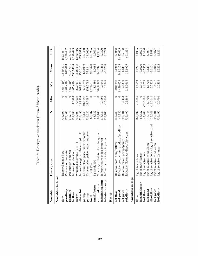
Tab
le7:
Des
crip
tive
stat
isti
cs(I
ntr
a-A
fric
antr
ade)
.
Vari
able
Desc
ripti
on
NM
inM
ax
Mean
S.D
.
Vari
able
sin
level
flow
Bilate
ral
trade
flow
736,4
90
04.6
5×
107
4,5
60.5
01
157,3
86.7
pro
dim
pP
roduct
ion
imp
ort
er172,8
66
04.6
7×
107
612,6
13
2,2
26,4
87
pro
dexp
Pro
duct
ion
exp
ort
er179,9
74
04.6
7×
107
610,4
87.1
2,1
87,5
05
intfl
ow
Inte
rnal
pro
duct
ion
139,2
80
1.1
893
4.6
5×
107
593,5
43.8
2,1
89,6
99
dis
twW
eighte
ddis
tance
(θ=
1)
736,4
90
18.9
908
962.9
211
3,5
48.4
38
1,9
62.7
16
dis
twin
tIn
tern
al
wei
ghte
ddis
tance
(θ=
1)
736,4
90
18.9
908
962.9
211
250.3
121
178.9
875
pcexp
Consu
mpti
on
pri
cein
dex
exp
ort
er716,1
49
21.5
687
858.5
782
63.1
952
49.9
450
pcim
pC
onsu
mpti
on
pri
cein
dex
imp
ort
er716,3
32
21.5
687
858.5
782
57.8
241
34.3
039
tari
ffT
ari
ff(%
)68,5
37
01,7
38.8
01
20.8
420
56.5
255
tari
fffa
cto
r1+
tari
ff/100
68,5
37
118.3
880
1.2
084
0.5
653
vol
bilat
exch
Vola
tility
of
bilate
ral
exch
ange
rate
59,1
66
0562,0
60.9
358.0
921
11,7
91.4
infr
ain
dex
imp
Infr
ast
ruct
ure
index
imp
ort
er118,6
34
-0.3
986
0.0
945
-0.3
215
0.0
820
infr
ain
dex
exp
Infr
ast
ruct
ure
index
imp
ort
er123,7
03
-0.3
986
0.0
945
-0.3
208
0.0
793
Rati
os
rel
flow
Rel
ati
ve
flow
:flow
/in
tflow
139,2
80
03,2
19.2
48
0.1
212
9.0
058
rel
pro
dR
elati
ve
pro
duct
ion:
pro
dex
p/pro
dim
p49,7
30
01,4
29,6
53
241.3
158
7,4
25.6
65
rel
pri
ce
Rel
ati
ve
pri
ce:
pce
xp/p
cim
p696,0
01
0.0
443
17.6
309
1.1
361
0.7
138
rel
dis
twR
elati
ve
dis
tance
:dis
tw/dis
twin
t736,4
90
0.9
269
514.5
665
32.1
975
60.4
278
Vari
able
sin
logs
lflow
log
of
trade
flow
s168,4
39
-6.9
695
17.6
553
3.9
221
3.1
385
lnta
riff
facto
rlo
gof
tari
fffa
ctor
68,5
37
02.9
117
0.1
670
0.1
624
lrel
flow
log
of
rela
tive
flow
47,2
08
-23.3
191
8.0
769
-6.5
959
4.3
440
lrel
pro
dlo
gof
rela
tive
pro
duct
ion
48,3
48
-14.1
729
14.1
729
0.1
351
3.0
901
dlr
el
flow
log
of
rela
tive
flow
-lo
gof
rela
tive
pro
d25,6
48
-19.0
141
5.7
305
-5.3
161
4.1
811
lrel
pri
ce
log
of
rela
tive
pro
duct
ion
696,0
01
-3.1
157
2.8
697
0.0
016
0.4
877
lrel
dis
twlo
gof
rela
tive
dis
tance
736,4
90
-0.0
760
6.2
433
2.7
272
1.1
291
32
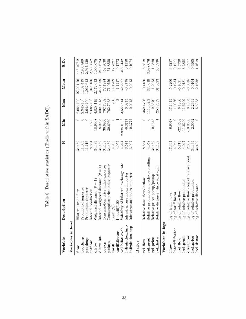
Tab
le8:
Des
crip
tive
stat
isti
cs(T
rad
ew
ith
inS
AD
C).
Vari
able
Desc
ripti
on
NM
inM
ax
Mean
S.D
.
Vari
able
sin
level
flow
Bilate
ral
trade
flow
34,4
39
02.6
8×
107
27,9
24.7
6445,4
07.2
pro
dim
pP
roduct
ion
imp
ort
er11,0
35
02.9
4×
107
1,1
02,4
19
2,9
80,8
09
pro
dexp
Pro
duct
ion
exp
ort
er11,1
16
02.9
4×
107
1,0
62,6
12
2,9
47,1
29
intfl
ow
Inte
rnal
pro
duct
ion
8,8
54
1.1
893
2.6
8×
107
1,0
45,1
66
2,6
93,8
52
dis
twW
eighte
ddis
tance
(θ=
1)
34,4
39
18.9
908
4,8
28.1
19
2,1
72.0
12
1,0
60.6
75
dis
twin
tIn
tern
al
wei
ghte
ddis
tance
(θ=
1)
34,4
39
18.9
908
802.9
943
343.1
269
240.4
223
pcexp
Consu
mpti
on
pri
cein
dex
exp
ort
er34,4
39
30.6
960
762.7
068
72.1
984
52.9
030
pcim
pC
onsu
mpti
on
pri
cein
dex
imp
ort
er34,4
39
30.6
960
762.7
068
71.0
756
51.8
350
tari
ffT
ari
ff(%
)4,9
55
0200
14.1
709
17.7
327
tari
fffa
cto
r1+
tari
ff/100
4,9
55
13
1.1
417
0.1
773
vol
bilat
exch
Vola
tility
of
bilate
ral
exch
ange
rate
4,2
44
2.9
9×
10−7
3,6
55.6
14
52.2
227
348.9
442
infr
ain
dex
imp
Infr
ast
ruct
ure
index
imp
ort
er3,5
74
-0.3
777
0.0
945
-0.2
778
0.1
150
infr
ain
dex
exp
Infr
ast
ruct
ure
index
imp
ort
er3,9
97
-0.3
777
0.0
945
-0.2
913
0.1
074
Rati
os
rel
flow
Rel
ati
ve
flow
:flow
/in
tflow
8,8
54
0462.4
796
0.4
180
6.5
818
rel
pro
dR
elati
ve
pro
duct
ion:
pro
dex
p/pro
dim
p4,0
58
0111,4
02.3
336.0
19
3,9
38.0
76
rel
pri
ce
Rel
ati
ve
pri
ce:
pce
xp/p
cim
p34,4
39
0.1
345
9.3
570
1.2
923
1.0
829
rel
dis
twR
elati
ve
dis
tance
:dis
tw/dis
twin
t34,4
39
1254.2
339
31.8
623
58.6
936
Vari
able
sin
logs
lflow
log
of
trade
flow
s17,3
64
-6.9
078
17.1
045
5.2
206
3.4
257
lnta
riff
facto
rlo
gof
tari
fffa
ctor
4,9
55
01.0
986
0.1
234
0.1
277
lrel
flow
log
of
rela
tive
flow
5,7
13
-22.4
508
6.1
366
-5.7
621
4.5
720
lrel
pro
dlo
gof
rela
tive
pro
duct
ion
4,0
47
-11.6
209
11.6
209
-0.0
181
3.2
858
dlr
el
flow
log
of
rela
tive
flow
-lo
gof
rela
tive
pro
d2,8
07
-13.9
850
3.4
003
-3.5
035
3.3
977
lrel
pri
ce
log
of
rela
tive
pro
duct
ion
34,4
39
-2.0
062
2.2
361
0.0
104
0.6
905
lrel
dis
twlo
gof
rela
tive
dis
tance
34,4
39
05.5
383
2.1
638
1.4
619
33
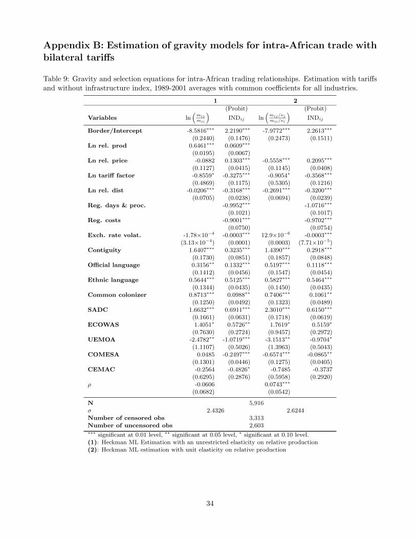
Appendix B: Estimation of gravity models for intra-African trade withbilateral tariffs
Table 9: Gravity and selection equations for intra-African trading relationships. Estimation with tariffsand without infrastructure index, 1989-2001 averages with common coefficients for all industries.
1 2
(Probit) (Probit)
Variables ln(mij
mii
)INDij ln
(mij/νjmii/νi
)INDij
Border/Intercept -8.5816∗∗∗ 2.2190∗∗∗ -7.9772∗∗∗ 2.2613∗∗∗
(0.2440) (0.1476) (0.2473) (0.1511)Ln rel. prod 0.6461∗∗∗ 0.0609∗∗∗
(0.0195) (0.0067)Ln rel. price -0.0882 0.1303∗∗∗ -0.5558∗∗∗ 0.2095∗∗∗
(0.1127) (0.0415) (0.1145) (0.0408)Ln tariff factor -0.8559∗ -0.3275∗∗∗ -0.9054∗ -0.3568∗∗∗
(0.4869) (0.1175) (0.5305) (0.1216)Ln rel. dist -0.0206∗∗∗ -0.3168∗∗∗ -0.2691∗∗∗ -0.3200∗∗∗
(0.0705) (0.0238) (0.0694) (0.0239)Reg. days & proc. -0.9952∗∗∗ -1.0716∗∗∗
(0.1021) (0.1017)Reg. costs -0.9001∗∗∗ -0.9702∗∗∗
(0.0750) (0.0754)Exch. rate volat. -1.78×10⁻⁴ -0.0003∗∗∗ 12.9×10⁻⁶ -0.0003∗∗∗
(3.13×10⁻⁴) (0.0001) (0.0003) (7.71×10⁻⁵)Contiguity 1.6407∗∗∗ 0.3235∗∗∗ 1.4390∗∗∗ 0.2918∗∗∗
(0.1730) (0.0851) (0.1857) (0.0848)Official language 0.3156∗∗ 0.1332∗∗∗ 0.5197∗∗∗ 0.1118∗∗∗
(0.1412) (0.0456) (0.1547) (0.0454)Ethnic language 0.5644∗∗∗ 0.5125∗∗∗ 0.5827∗∗∗ 0.5464∗∗∗
(0.1344) (0.0435) (0.1450) (0.0435)Common colonizer 0.8713∗∗∗ 0.0988∗∗ 0.7406∗∗∗ 0.1061∗∗
(0.1250) (0.0492) (0.1323) (0.0489)SADC 1.6632∗∗∗ 0.6911∗∗∗ 2.3010∗∗∗ 0.6150∗∗∗
(0.1661) (0.0631) (0.1718) (0.0619)ECOWAS 1.4051∗ 0.5726∗∗ 1.7619∗ 0.5159∗
(0.7630) (0.2724) (0.9457) (0.2972)UEMOA -2.4782∗∗ -1.0719∗∗∗ -3.1513∗∗ -0.9704∗
(1.1107) (0.5026) (1.3963) (0.5043)COMESA 0.0485 -0.2497∗∗∗ -0.6574∗∗∗ -0.0865∗∗
(0.1301) (0.0446) (0.1275) (0.0405)CEMAC -0.2564 -0.4826∗ -0.7485 -0.3737
(0.6295) (0.2876) (0.5958) (0.2920)ρ -0.0606 0.0743∗∗∗
(0.0682) (0.0542)
N 5,916σ 2.4326 2.6244Number of censored obs 3,313Number of uncensored obs 2,603∗∗∗ significant at 0.01 level, ∗∗ significant at 0.05 level, ∗ significant at 0.10 level.(1): Heckman ML Estimation with an unrestricted elasticity on relative production(2): Heckman ML estimation with unit elasticity on relative production
34
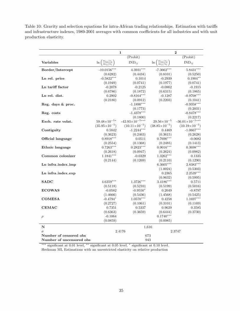
Table 10: Gravity and selection equations for intra-African trading relationships. Estimation with tariffsand infrastructure indexes, 1989-2001 averages with common coefficients for all industries and with unitproduction elasticity.
1 2
(Probit) (Probit)
Variables ln(mij/νjmii/νi
)INDij ln
(mij/νjmii/νi
)INDij
Border/Intercept -10.0156∗∗∗ 4.3931∗∗∗ -7.3662∗∗∗ 5.8431∗∗∗
(0.6282) (0.4434) (0.8101) (0.5250)Ln rel. price -0.5822∗∗∗ 0.1014 -0.2939 0.1904∗∗
(0.1949) (0.0741) (0.1977) (0.0741)Ln tariff factor -0.2078 -0.2125 -0.0862 -0.1915
(0.6786) (0.1872) (0.6315) (0.1865)Ln rel. dist. 0.2902 -0.8164∗∗∗ -0.1287 -0.9708∗∗∗
(0.2180) (0.0912) (0.2203) (0.1041)Reg. days & proc. -1.1890∗∗∗ -0.9358∗∗∗
(0.1773) (0.2031)Reg. costs -1.4378∗∗∗ -0.8478∗∗∗
(0.1800) (0.2217)Exch. rate volat. 59.48×10⁻⁵∗ -42.93×10⁻⁵∗∗∗ 29.56×10⁻⁵ -36.01×10⁻⁵∗∗∗
(35.95×10⁻⁵) (10.11×10⁻⁵) (38.85×10⁻⁵) (10.19×10⁻⁵)Contiguity 0.5842 -1.2244∗∗∗ 0.4469 -1.0667∗∗∗
(0.3623) (0.2463) (0.3615) (0.2628)Official language 0.8918∗∗∗ 0.0511 0.7690∗∗∗ -0.0682
(0.2554) (0.1368) (0.2485) (0.1413)Ethnic language 0.7263∗∗∗ 0.2823∗∗∗ 0.9016∗∗∗ 0.3698∗∗∗
(0.2618) (0.0947) (0.2624) (0.0982)Common colonizer 1.1841∗∗∗ -0.0329 1.3262∗∗∗ 0.1335
(0.2144) (0.1269) (0.2110) (0.1290)Ln infra index imp 6.3605∗∗∗ 2.8383∗∗∗
(1.0024) (0.5303)Ln infra index exp 0.2365 2.2539∗∗∗
(0.9632) (0.5995)SADC 4.6359∗∗∗ 1.3726∗∗∗ 3.4186∗∗∗ 0.5711
(0.5118) (0.5210) (0.5199) (0.5016)ECOWAS -0.0582 -0.9550∗ 0.2049 -0.8797
(1.4666) (0.5436) (1.4568) (0.5425)COMESA -0.4794∗ 1.0570∗∗∗ 0.4258 1.1697∗∗∗
(0.2727) (0.1061) (0.3101) (0.1169)CEMAC 0.7351 0.5337 0.9629 0.3585
(0.6363) (0.3659) (0.6444) (0.3730)ρ -0.1064 0.1740∗∗∗
(0.0859) (0.0985)
N 1,616σ 2.4176 2.3747Number of censored obs 673Number of uncensored obs 943∗∗∗ significant at 0.01 level, ∗∗ significant at 0.05 level, ∗ significant at 0.10 level.Heckman ML Estimations with an unrestricted elasticity on relative production
35
Related Documents