1 The 2 k Factorial Design • Montgomery, chap 6; BHH (2nd ed), chap 5 • Special case of the general factorial design; k factors, all at two levels • Require relatively few runs per factor studied • Very widely used in industrial experimentation • Interpretation of data can proceed largely by common sense, elementary arithmetic, and graphics • For quantitative factors, can’t explore a wide region of factor space, but determine promising directions • Designs can be suitably augmented---sequential assembly • Basis for 2-level fractional fractorial designs, especially useful for screening.

Welcome message from author
This document is posted to help you gain knowledge. Please leave a comment to let me know what you think about it! Share it to your friends and learn new things together.
Transcript

1
The 2k Factorial Design• Montgomery, chap 6; BHH (2nd ed), chap 5• Special case of the general factorial design; k factors, all at two levels• Require relatively few runs per factor studied• Very widely used in industrial experimentation• Interpretation of data can proceed largely by common sense, elementary
arithmetic, and graphics• For quantitative factors, can’t explore a wide region of factor space, but
determine promising directions• Designs can be suitably augmented---sequential assembly• Basis for 2-level fractional fractorial designs, especially useful for
screening.

2
The Simplest Case: The 22
“-” and “+” denote the low and high levels of a factor, respectively.
Note names of treatment combinations: (1), a, b, ab
Low and high are arbitrary terms
Geometrically, the four runs form the corners of a square
Factors: quantitative or qualitative; interpretation in the final model will be different
3
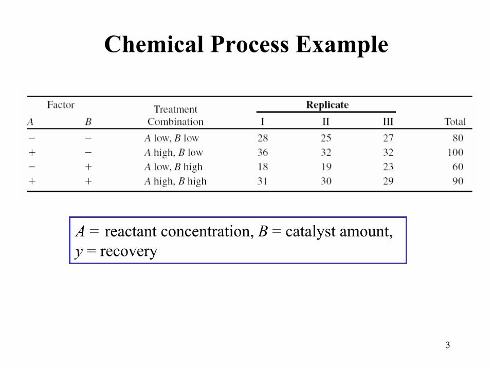
Chemical Process Example
A = reactant concentration, B = catalyst amount, y = recovery

4
Analysis Procedure for a Factorial Design
• Estimate factor effects• Formulate model
– With replication, use full model– With an unreplicated design, use normal probability
plots• Statistical testing (ANOVA)• Refine the model• Analyze residuals (graphical)• Interpret results
5
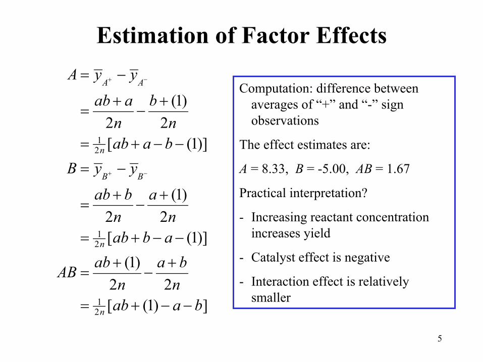
Estimation of Factor Effects
12
12
12
(1)2 2[ (1)]
(1)2 2[ (1)]
(1)2 2[ (1) ]
A A
n
B B
n
n
A y y
ab a bn nab a b
B y y
ab b an nab b a
ab a bABn n
ab a b
+ −
+ −
= −
+ += −
= + − −
= −
+ += −
= + − −
+ += −
= + − −
Computation: difference between averages of “+” and “-” sign observations
The effect estimates are:
A = 8.33, B = -5.00, AB = 1.67
Practical interpretation?
- Increasing reactant concentration increases yield
- Catalyst effect is negative
- Interaction effect is relatively smaller

6
Statistical Testing - ANOVA

7
Residuals and Diagnostic Checking

8
The Response Surface(for the additive model)
9
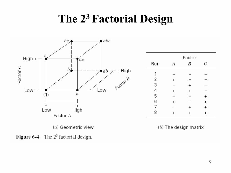
The 23 Factorial Design

10
Effects in The 23 Factorial Design
etc, etc, ...
A A
B B
C C
A y y
B y y
C y y
+ −
+ −
+ −
= −
= −
= −
Interaction effects are also differences between averages of 4 runs.
11
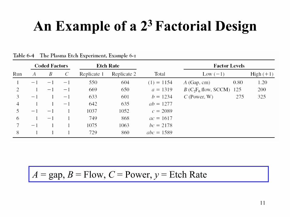
An Example of a 23 Factorial Design
A = gap, B = Flow, C = Power, y = Etch Rate

12
Table of – and + Signs for the 23 Factorial Design (pg. 214)

13
Properties of the Table • Except for column I, every column has an equal number of + and –
signs• The sum of the product of signs in any two columns is zero:
orthogonal design• Multiplying any column by I leaves that column unchanged (identity
element)• The product of any two columns yields a column in the table:
• Orthogonality is an important property shared by all factorial designs
2
A B ABAB BC AB C AC× =
× = =
14
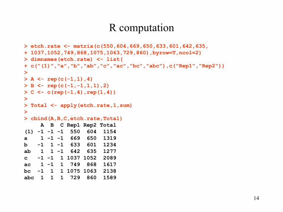
R computation> etch.rate <- matrix(c(550,604,669,650,633,601,642,635,+ 1037,1052,749,868,1075,1063,729,860),byrow=T,ncol=2)> dimnames(etch.rate) <- list(+ c("(1)","a","b","ab","c","ac","bc","abc"),c("Rep1","Rep2"))> > A <- rep(c(-1,1),4)> B <- rep(c(-1,-1,1,1),2)> C <- c(rep(-1,4),rep(1,4))> > Total <- apply(etch.rate,1,sum)> > cbind(A,B,C,etch.rate,Total)
A B C Rep1 Rep2 Total(1) -1 -1 -1 550 604 1154a 1 -1 -1 669 650 1319b -1 1 -1 633 601 1234ab 1 1 -1 642 635 1277c -1 -1 1 1037 1052 2089ac 1 -1 1 749 868 1617bc -1 1 1 1075 1063 2138abc 1 1 1 729 860 1589
15
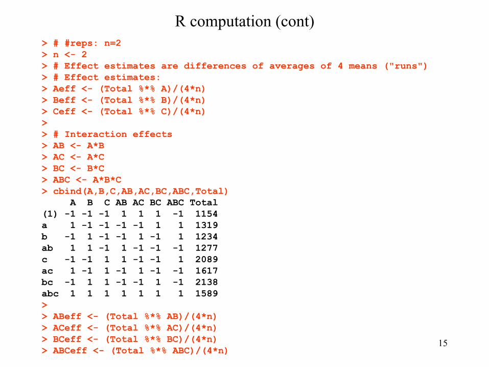
R computation (cont)> # #reps: n=2> n <- 2> # Effect estimates are differences of averages of 4 means ("runs")> # Effect estimates:> Aeff <- (Total %*% A)/(4*n)> Beff <- (Total %*% B)/(4*n)> Ceff <- (Total %*% C)/(4*n)> > # Interaction effects> AB <- A*B> AC <- A*C> BC <- B*C> ABC <- A*B*C> cbind(A,B,C,AB,AC,BC,ABC,Total)
A B C AB AC BC ABC Total(1) -1 -1 -1 1 1 1 -1 1154a 1 -1 -1 -1 -1 1 1 1319b -1 1 -1 -1 1 -1 1 1234ab 1 1 -1 1 -1 -1 -1 1277c -1 -1 1 1 -1 -1 1 2089ac 1 -1 1 -1 1 -1 -1 1617bc -1 1 1 -1 -1 1 -1 2138abc 1 1 1 1 1 1 1 1589> > ABeff <- (Total %*% AB)/(4*n)> ACeff <- (Total %*% AC)/(4*n)> BCeff <- (Total %*% BC)/(4*n)> ABCeff <- (Total %*% ABC)/(4*n)

16
R computation (cont)> # Summary> Effects <- t(Total) %*% cbind(A,B,C,AB,AC,BC,ABC)/(4*n)> Summary <- rbind( cbind(A,B,C,AB,AC,BC,ABC),Effects )> dimnames(Summary)[[1]] <- c(dimnames(etch.rate)[[1]],"Effect")> Summary
A B C AB AC BC ABC(1) -1.000 -1.000 -1.000 1.000 1.000 1.000 -1.000a 1.000 -1.000 -1.000 -1.000 -1.000 1.000 1.000b -1.000 1.000 -1.000 -1.000 1.000 -1.000 1.000ab 1.000 1.000 -1.000 1.000 -1.000 -1.000 -1.000c -1.000 -1.000 1.000 1.000 -1.000 -1.000 1.000ac 1.000 -1.000 1.000 -1.000 1.000 -1.000 -1.000bc -1.000 1.000 1.000 -1.000 -1.000 1.000 -1.000abc 1.000 1.000 1.000 1.000 1.000 1.000 1.000Effect -101.625 7.375 306.125 -24.875 -153.625 -2.125 5.625> > # Fit as an ANOVA model> etch.vec <- c(t(etch.rate))> Af <- rep(as.factor(A),rep(2,8))> Bf <- rep(as.factor(B),rep(2,8))> Cf <- rep(as.factor(C),rep(2,8))> options(contrasts=c("contr.sum","contr.poly"))> etch.lm <- lm(etch.vec ~ Af*Bf*Cf)

17
Estimation of Factor Effects

18
Model Coefficients – Full Model

19
R computation (cont)> options(contrasts=c("contr.sum","contr.poly"))> etch.lm <- lm(etch.vec ~ Af*Bf*Cf)> summary(etch.lm)
Call:lm(formula = etch.vec ~ Af * Bf * Cf)
Residuals:Min 1Q Median 3Q Max
-6.550e+01 -1.113e+01 8.882e-16 1.113e+01 6.550e+01
Coefficients:Estimate Std. Error t value Pr(>|t|)
(Intercept) 776.062 11.865 65.406 3.32e-12 ***Af1 50.813 11.865 4.282 0.002679 ** Bf1 -3.687 11.865 -0.311 0.763911 Cf1 -153.062 11.865 -12.900 1.23e-06 ***Af1:Bf1 -12.437 11.865 -1.048 0.325168 Af1:Cf1 -76.812 11.865 -6.474 0.000193 ***Bf1:Cf1 -1.063 11.865 -0.090 0.930849 Af1:Bf1:Cf1 -2.812 11.865 -0.237 0.818586 ---Signif. codes: 0 '***' 0.001 '**' 0.01 '*' 0.05 '.' 0.1 ' ' 1
Residual standard error: 47.46 on 8 degrees of freedomMultiple R-Squared: 0.9661, Adjusted R-squared: 0.9364 F-statistic: 32.56 on 7 and 8 DF, p-value: 2.896e-05
Review question:
Why are the anovamodel coefficients ½the “effect estimates”?

20
ANOVA Summary – Full Model

21
R computation (cont)> anova(etch.lm)Analysis of Variance Table
Response: etch.vecDf Sum Sq Mean Sq F value Pr(>F)
Af 1 41311 41311 18.3394 0.0026786 ** Bf 1 218 218 0.0966 0.7639107 Cf 1 374850 374850 166.4105 1.233e-06 ***Af:Bf 1 2475 2475 1.0988 0.3251679 Af:Cf 1 94403 94403 41.9090 0.0001934 ***Bf:Cf 1 18 18 0.0080 0.9308486 Af:Bf:Cf 1 127 127 0.0562 0.8185861 Residuals 8 18020 2253 ---Signif. codes: 0 '***' 0.001 '**' 0.01 '*' 0.05 '.' 0.1 ' ' 1 > model.matrix(etch.lm)
(Intercept) Af1 Bf1 Cf1 Af1:Bf1 Af1:Cf1 Bf1:Cf1 Af1:Bf1:Cf11 1 1 1 1 1 1 1 12 1 1 1 1 1 1 1 13 1 -1 1 1 -1 -1 1 -14 1 -1 1 1 -1 -1 1 -15 1 1 -1 1 -1 1 -1 -16 1 1 -1 1 -1 1 -1 -17 1 -1 -1 1 1 -1 -1 18 1 -1 -1 1 1 -1 -1 19 1 1 1 -1 1 -1 -1 -110 1 1 1 -1 1 -1 -1 -111 . . .

22
BHH sect 5.10: “Misuse of the ANOVA for 2k
Factorial Experiments”
• For 2k designs, the use of the ANOVA is confusing and makes little sense. N=n×2k observations. 2k -1 d.f. partitioned into individual “SS” for effects, each equal to N(effect)2/4, divided by df=1, and turned into an F-ratio. Experimenter wants magnitude of effect, , and t ratio = effect/se(effect).
• P-values should not be used mechanically for yes-or-no decisions on what effects are real. Information about the size of an effect and its possible error must be allowed to interact with experimenter’s subject matter knowledge. Graphical methods (coming) provide a valuable means of allowing information in the data and in the mind of the experimenter to interact properly.
y y+ −−

23
Refine Model – Remove Nonsignificant Factors
Note that Sums of Squares for A, C, AC did not change.

24
Model Coefficients – Reduced Model
What has changed from the previous larger table of coefficient estimates?

25
Model Summary Statistics for Reduced Model (pg. 222)
• R2 and adjusted R2
• R2 for prediction (based on PRESS)
52
5
25
5.106 10 0.96085.314 10
/ 20857.75 /121 1 0.9509/ 5.314 10 /15
Model
T
E EAdj
T T
SSRSS
SS dfRSS df
×= = =
×
= − = − =×
2Pred 5
37080.441 1 0.93025.314 10T
PRESSRSS
= − = − =×

26
Model Summary Statistics (pg. 222)
• Standard error of model coefficients (full model)
• Confidence interval on model coefficients
2 2252.56ˆ ˆ( ) ( ) 11.872 2 2(8)
Ek k
MSse Vn nσβ β= = = = =
/ 2, / 2,ˆ ˆ ˆ ˆ( ) ( )
E Edf dft se t seα αβ β β β β− ≤ ≤ +
Exercise: derive the above expression for
β̂
ˆ( )se β
27
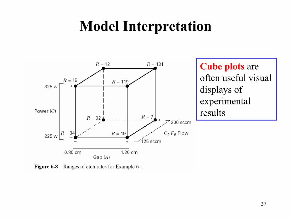
Model Interpretation
Cube plots are often useful visual displays of experimental results
28
Assessing “error” or residual variation
Often there are more factors to be investigated that can conveniently be accommodated with the time and budget available. Rather than make 16 runs for a replicated 23
factorial, it might be preferable to introduce a 4th factor and run an un-replicated 24 design.
Options:1.With replication, use the usual pooled variance computed from the replicates.2.Assume that higher order interaction effects are noise and construct and internal reference set.3.Assess meaningful effects, including possibly meaningful higher order interactions, using Normal and “Lenth” plots.

29
Example: Process development experiment.
Response: “percent conversion”
Factor Level 1 Level 2Catalyst charge (lb) 10 15Temperature © 220 240Pressure (psi) 50 80Reactant concentration (%) 10 12
> # Read in process development data of BHH2 Table 5.10a> tab5.10.dat <- read.table(file.choose(),header=T)> dimnames(tab5.10.dat)[[2]][2:5] <- c("A","B","C","D")> tab5.10.dat
yatesOrd A B C D conversion randomOrd1 1 -1 -1 -1 -1 70 82 2 1 -1 -1 -1 60 23 3 -1 1 -1 -1 89 104 4 1 1 -1 -1 81 45 5 -1 -1 1 -1 69 156 6 1 -1 1 -1 62 97 7 -1 1 1 -1 88 18 8 1 1 1 -1 81 139 9 -1 -1 -1 1 60 1610 10 1 -1 -1 1 49 511 11 -1 1 -1 1 88 1112 12 1 1 -1 1 82 1413 13 -1 -1 1 1 60 314 14 1 -1 1 1 52 1215 15 -1 1 1 1 86 616 16 1 1 1 1 79 7

30
> # Full design matrix with interactions> des4 <- ffFullMatrix(X,x=c(1,2,3,4),maxInt=4)> des4$Xa
one x1 x2 x3 x4 x1*x2 x1*x3 x1*x4 x2*x3 x2*x4 x3*x4 x1*x2*x3 x1*x2*x41 1 -1 -1 -1 -1 1 1 1 1 1 1 -1 -12 1 1 -1 -1 -1 -1 -1 -1 1 1 1 1 13 1 -1 1 -1 -1 -1 1 1 -1 -1 1 1 14 1 1 1 -1 -1 1 -1 -1 -1 -1 1 -1 -15 1 -1 -1 1 -1 1 -1 1 -1 1 -1 1 -16 1 1 -1 1 -1 -1 1 -1 -1 1 -1 -1 17 1 -1 1 1 -1 -1 -1 1 1 -1 -1 -1 18 1 1 1 1 -1 1 1 -1 1 -1 -1 1 -19 1 -1 -1 -1 1 1 1 -1 1 -1 -1 -1 110 1 1 -1 -1 1 -1 -1 1 1 -1 -1 1 -111 1 -1 1 -1 1 -1 1 -1 -1 1 -1 1 -112 1 1 1 -1 1 1 -1 1 -1 1 -1 -1 113 1 -1 -1 1 1 1 -1 -1 -1 -1 1 1 114 1 1 -1 1 1 -1 1 1 -1 -1 1 -1 -115 1 -1 1 1 1 -1 -1 -1 1 1 1 -1 -116 1 1 1 1 1 1 1 1 1 1 1 1 1[. . . additional columns of 1’s and -1’s . . . ]
$x[1] 1 2 3 4$maxInt[1] 4$nTerms
blk main int.2 int.3 int.4 0 4 6 4 1

31
> # Use the higher order interaction effects as the reference set of> # (independent) effects that represent noise. The standard > # deviation of these (about zero) provides a relevant se for > # the rest of the effects.> > Xeffects <- matrix(tab5.10.dat$conversion,nrow=1) %*% des4$Xa[,-1]/8> dotPlot(Xeffects[1:10])> dots(Xeffects[11:15],y=0.1,stacked=T,pch=19) # add the higher order effects> SEeffect <- sqrt(sum(Xeffects[11:15]^2)/5)> SEeffect[1] 0.5477226> lines(SEeffect*seq(-10,10,.11),dt(seq(-10,10,.11),df=5)) # add t(df=5) reference density> t.ratios <- Xeffects[11:15]/SEeffect> round(t.ratios,2)[1] -1.37 0.91 -0.46 -1.37 -0.46
> # The "significant" design effects relative to the higher> # order interactions as a reference set are clear are clear.
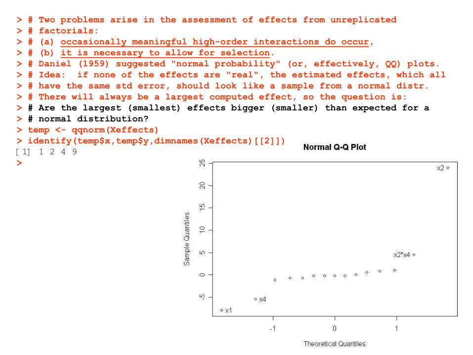
32
> # Two problems arise in the assessment of effects from unreplicated> # factorials:> # (a) occasionally meaningful high-order interactions do occur,> # (b) it is necessary to allow for selection.> # Daniel (1959) suggested "normal probability" (or, effectively, QQ) plots.> # Idea: if none of the effects are "real", the estimated effects, which all> # have the same std error, should look like a sample from a normal distr.> # There will always be a largest computed effect, so the question is: > # Are the largest (smallest) effects bigger (smaller) than expected for a> # normal distribution?> temp <- qqnorm(Xeffects)> identify(temp$x,temp$y,dimnames(Xeffects)[[2]])[1] 1 2 4 9>

33
> # If we were correct in assessing the standard error of the effects from the> # higher order interactions, as above, then the a line with slop SEeffect> # should characterize the appropriate std dev (slope of the qqplot)> # for the majority of the effects.> abline(0,.55)
34
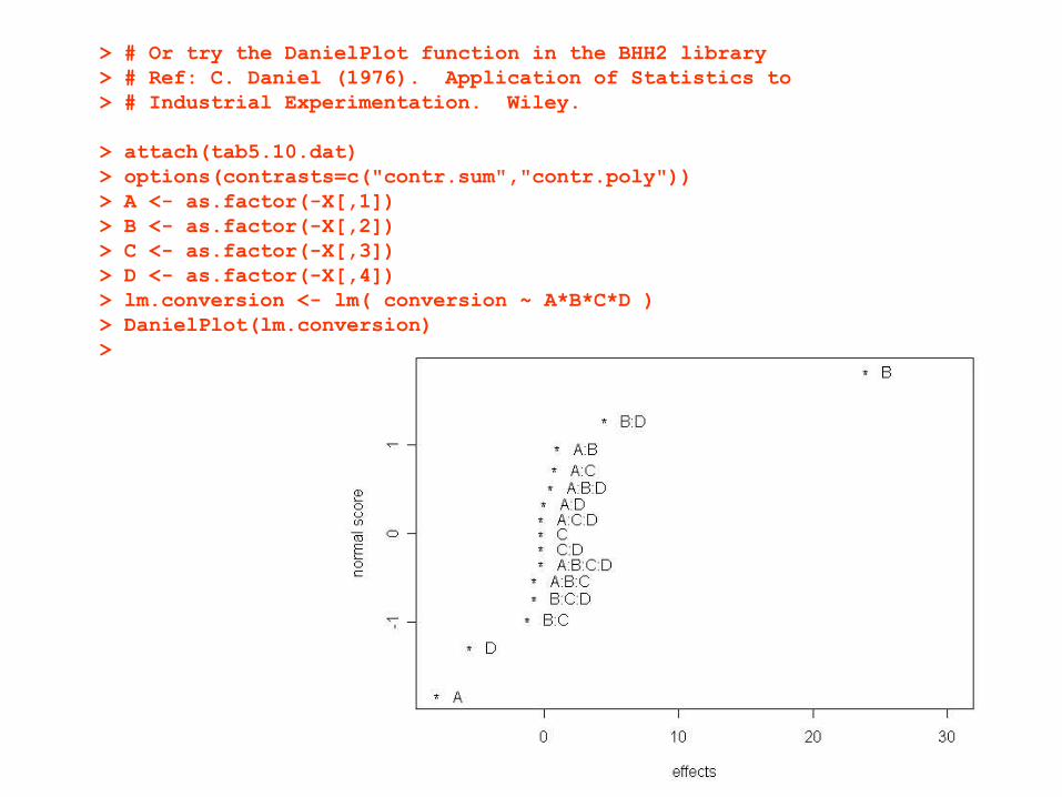
> # Or try the DanielPlot function in the BHH2 library> # Ref: C. Daniel (1976). Application of Statistics to> # Industrial Experimentation. Wiley.
> attach(tab5.10.dat)> options(contrasts=c("contr.sum","contr.poly"))> A <- as.factor(-X[,1])> B <- as.factor(-X[,2])> C <- as.factor(-X[,3])> D <- as.factor(-X[,4])> lm.conversion <- lm( conversion ~ A*B*C*D )> DanielPlot(lm.conversion)>
35
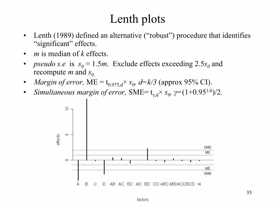
Lenth plots• Lenth (1989) defined an alternative (“robust”) procedure that identifies
“significant” effects.• m is median of k effects. • pseudo s.e is s0 = 1.5m. Exclude effects exceeding 2.5s0 and
recompute m and s0.
• Margin of error, ME = t0.975,d× s0, d=k/3 (approx 95% CI).• Simultaneous margin of error, SME= tγ,d× s0, γ=(1+0.951/k)/2.

36
> # Diagnostic plotting of residuals> # Fit without identified "significant" effects
> lm.sub.conversion <- lm(conversion ~ des4$Xa[,c("x1","x2","x4","x2*x4")])
> par(mfrow=c(1,2))> plot(fitted(lm.sub.conversion),resid(lm.sub.conversion))> abline(h=0,lty=2)> qqnorm(resid(lm.sub.conversion))> qqline(resid(lm.sub.conversion))
37
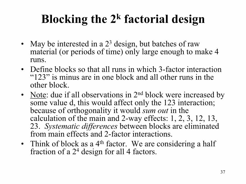
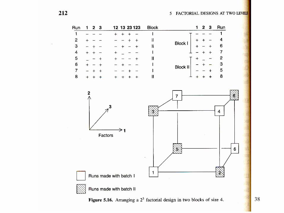
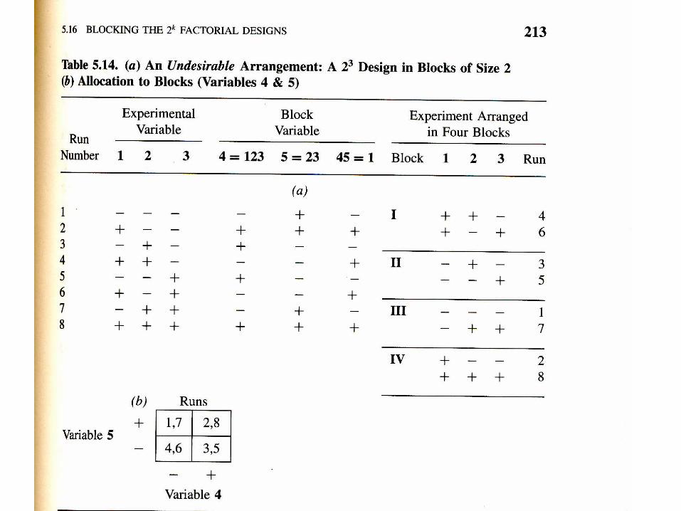
Blocking the 2k factorial design
• May be interested in a 23 design, but batches of raw material (or periods of time) only large enough to make 4 runs.
• Define blocks so that all runs in which 3-factor interaction “123” is minus are in one block and all other runs in the other block.
• Note: due if all observations in 2nd block were increased by some value d, this would affect only the 123 interaction; because of orthogonality it would sum out in the calculation of the main and 2-way effects: 1, 2, 3, 12, 13, 23. Systematic differences between blocks are eliminated from main effects and 2-factor interactions.
• Think of block as a 4th factor. We are considering a half fraction of a 24 design for all 4 factors.
38
39
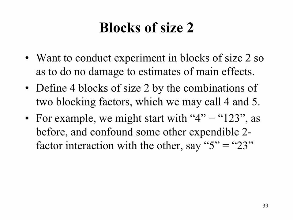
Blocks of size 2
• Want to conduct experiment in blocks of size 2 so as to do no damage to estimates of main effects.
• Define 4 blocks of size 2 by the combinations of two blocking factors, which we may call 4 and 5.
• For example, we might start with “4” = “123”, as before, and confound some other expendible 2-factor interaction with the other, say “5” = “23”
40

41
Generators and defining relations
• We write I for the vector of 1’s, and the product of any design column with itself is I=11=22=33=44=55
• Take the two specifications for the blocking variables, 4=123 and 5=23. Multiply 1st expresion by 4 and 2nd by 5: I=1234 and I=235. These are called the generators of the blocking arrangements.
• Multiply these two together and to get 1223345=145 to complete the defining relation I=1234=235=145.
• The third generator shows that the main effect 1 is confounded with the 45 block effect, which we don’t want.
• Better: confound the two block variables 4 and 5 with any two of the 2-factor interactions, say 4=12, 5=13

42

43
Fractional Factorial Designs• Chapter 6 of BHH (2nd ed) discusses fractional factorial
designs.• Example: full 25 factorial would require 32 runs. An
experiment with only 8 runs is a 1/4th (quarter) fraction. Because ¼=(½)2=2-2, this is referred to as a 25-2 design.
• In general, 2k-p design is a (½)p fraction of a 2k design using 2k-p runs.
• Note that the first blocked design we considered was a half fraction: 24-1 defined by the generating relation I=1234, which provides all the confounded (“aliased”) relationships. E.g. 1=1I=11234=234.
Related Documents