That BLUP is a Good Thing: The Estimation of Random … · mal breeding. It is a method of estimating random BLUP estimates of the realized values of the random variables u are linear

That BLUP is a Good Thing: The Estimation of Random Effects

G. K. Robinson

Statistical Science, Vol. 6, No. 1. (Feb., 1991), pp. 15-32.

Stable URL:

http://links.jstor.org/sici?sici=0883-4237%28199102%296%3A1%3C15%3ATBIAGT%3E2.0.CO%3B2-%23

Statistical Science is currently published by Institute of Mathematical Statistics.

Your use of the JSTOR archive indicates your acceptance of JSTOR's Terms and Conditions of Use, available athttp://www.jstor.org/about/terms.html. JSTOR's Terms and Conditions of Use provides, in part, that unless you have obtainedprior permission, you may not download an entire issue of a journal or multiple copies of articles, and you may use content inthe JSTOR archive only for your personal, non-commercial use.

Please contact the publisher regarding any further use of this work. Publisher contact information may be obtained athttp://www.jstor.org/journals/ims.html.

Each copy of any part of a JSTOR transmission must contain the same copyright notice that appears on the screen or printedpage of such transmission.

The JSTOR Archive is a trusted digital repository providing for long-term preservation and access to leading academicjournals and scholarly literature from around the world. The Archive is supported by libraries, scholarly societies, publishers,and foundations. It is an initiative of JSTOR, a not-for-profit organization with a mission to help the scholarly community takeadvantage of advances in technology. For more information regarding JSTOR, please contact [email protected].

http://www.jstor.orgTue Sep 18 13:58:31 2007

http://links.jstor.org/sici?sici=0883-4237%28199102%296%3A1%3C15%3ATBIAGT%3E2.0.CO%3B2-%23

http://www.jstor.org/about/terms.html

http://www.jstor.org/journals/ims.html

Statistical Science 1991,Vol. 6 , No.1, 15-61

That BLUP Is a Good Thing: The Estimation of Random Effects G. K. Robinson .

Abstract. In animal breeding, Best Linear Unbiased Prediction, or BLUP, is a technique for estimating genetic merits. In general, it is a method of estimating random effects. It can be used to derive the Kalman filter, the method of Kriging used for ore reserve estimation, credibility theory used to work out insurance premiums, and Hoadley's quality measurement plan used to estimate a quality index. It can be used for removing noise from images and for small-area estimation. This paper presents the theory of BLUP, some examples of its application and its relevance to the foundations of statistics.

Understanding of procedures for estimating random effects should help people to understand some complicated and controversial issues about fixed and random effects models and also help to bridge the apparent gulf between the Bayesian and Classical schools of thought.

Key words and phrases: Best linear unbiased prediction (BLUP), estimation of random effects, fixed versus random effects, foundations of statistics, likelihood, selection index, Kalman filtering, parametric empirical Bayes methods, small-area estimation, credibility theory, ranking and selection.

1. INTRODUCTION R depend. Generally, it will be assumed that the

The acronym BLUP stands for "Best Linear Un- variance-covariance structure is known except per-

biased Prediction" and is in common usage in ani- haps for the single parameter a2.

mal breeding. It is a method of estimating random BLUP estimates of the realized values of the random variables u are linear in the sense that

effects. they are linear functions of the data, y; unbiased The context of BLUP is the linear model in the sense that the average value of the estimate

is equal to the average value of the quantity being estimated; best in the sense that they have mini-

where y is a vector of n observable random vari- mum mean squared error within the class of linear ables, /3 is a vector of p unknown parameters unbiased estimators; and predictors to distinguish having fixed values (fixed effects), X and Z are them from estimators of fixed effects. A convention known matrices, and u and e are vectors of q and 'has somehow developed that estimators of random n, respectively, unobservable random variables effects are called predictors while estimators of (random effects) such that E(u) = 0, E(e) = 0 and fixed effects are called estimators. As discussed in

Section 7.1, I prefer to use the term "estimators" for both fixed and random effects.

Mathematically, the BLUP estimates 8 of /3 andwhere G and R are known positive definite matri- 2 of u are defined as solutions to the following ces and a2 is a positive constant. simultaneous equations which were given by Hen-

At times, we will discuss the estimation of disper- derson (1950), although in summation rather than sion parameters and will use 0 to denote a vector of matrix form: dispersion parameters on which the matrices G and

G. K. Robinson is Principal Research Scientist, CSIRO, Division of Mathematics and Statistics, Pri- vate Bag 10, Clayton Victoria 3168, Australia. These equations have sometimes been called

16 G. K. ROBINSON

"mixed model equations,', and f? and ii referred to where sj is the effect of the j th sire on his daugh- as "mixed model solutions." Note that as G-' tends ters' lactation yields, to the zero matrix these equations tend formally to the generalized least-squares equations for estimating 0 and u when the components of u are regarded as fixed .effects.

Henderson (1975)showed that provided X is of full rank, p, the variance-covariance matrix of estimation errors is

.[["qT}61["ii-u ii-u

That BLUP estimates generally differ from the generalized least squares estimates that would be used if u were regarded as fixed is illustrated by the following example.

EXAMPLE.A simple example of model (1.1)is that of first lactation yields of dairy cows with sire additive genetic merits being treated as random effects (u)and herd effects being treated as fixed effects (6).The matrix R a 2 is the variance- covariance matrix of the vector e of departures from a model in which yield was explicable entirely by sire effects and herd effects. The matrix R will be taken to be the identity matrix. Assume that the matrix G is a known multiple of the identity matrix, say 0.1I. This would be a reasonable assumption provided that the sires were unrelated and provided that the variance ratio had been estimated previously.

Suppose that we' had records as follows.

Herd Sire Yield

1 A 110 1 D 100 2 B 110 2 D 100 2 D 100 3 c . 110 3 C 110 3 D 100 3 D 100

Then the entities in equation (1.1)are

where hi is the environmental effect of the ith herd,

'1 0 0' 1 0 0 0 1 0 0 1 0

X = O l O 0 0 1 0 0 1

and

Z =

Equation (1.2)gives us

which has solution

If sire effects were treated as fixed, then equation (1.2)would be changed by omission of G- l. This means that the last four diagonal elements in the left-hand-side matrix of equation (1.3)w_ould be reduced by 10.The matrix equation for /3 and ii would no longer be of full rank, but a solution can

17 THE ESTIMATION OF RANDOM EFFECTS

be obtained by setting, arbitrarily, s, = 0. This solution is

The solution given by (1.5) is the least-squares solution with which most statisticians are well ac- quainted. Intuitively, each of the sires other than D has daughters that yield 10 units more on average than the daughters of sire D to which they can be directly compared.

The BLUP solution given by (1.4) takes into account the information that sire effects have less variation than the variance of lactation yields from daughters of a single sire. The extent to which a sire's estimated genetic merit is regressed toward the mean depends on the amount of information available concerning that sire. For instance, sire C is estimated to be better than sires A and B be-cause more is known about him-the lactation yields of his daughters are the same (110) as those of sires A and B.

The variance-covariance matrix of the estimates from the mixed model is u 2 times the inverse of the left-hand-side matrix in equation (1.3). The diagonal elements of the inverse matrix for s,, s,, s, and s, are 0.0954, 0.0941, 0.0916 and 0.0833, respectively. Since the merit of a sire about which nothing was known would have a variance of 0.1 u2, there has been little gain in precision of sire effect estimates due to data on lactations of daughters.

REMARKS.In this example, numbers with few significant digits have been used in order to make the example easier to follow. Consequently, variance parameters should not be estimated from the given data. In practical situations, the variance ratio that was taken to be 0.1 or the variance u 2 may need to be estimated from the same data as is used to estimate sire genetic merits.

My introduction to the estimation of random effects was as statisician for the Australian Dairy Qerd Improvement Scheme in mid-1980. This means that I think first of the estimation of genetic merits of dairy cattle when I think of estimating random effects. Readers might like to allow for this point of view.

2. OBJECTIVES

In a discussion at the ~ o i a l Statistical Society, Dawid (1976) remarked

A constant theme in the development of statistics has been the search for justification for

what statisticians do. To read the textbooks, one might get the distorted idea that 'Student' proposed his t-test because it was the Uni- formly Most Powerful Unbiased test for a Nor- mal mean, but it would be more accurate to say that the concept of UMPU gains much of its appeal because it produces the t-test, and ev- eryone knows that the t-test is a good thing.

The words "a good thing" in the title of this paper are to be interpreted as coming from this quotation. I wish to argue that the BLUP method for estimating random effects is "a good thing" just as Student's t-test is "a good thing."

I believe that the Classical school of thought in statistical inference should accept estimation of random effects as a legitimate activity. This theme will be developed in Section 4.3, which gives a classical justification for BLUP, and in Section 6, which lists applications. If estimation of random effects were accepted as legitimate by the Classical school, then the Bayesian and Classical schools of thought in statistics would differ less than much current rhetoric suggests.

Another objective is to encourage communication between people who deal with the various applications where random effects are estimated. The 50th Anniversary Conference, Iowa State Statistical Laboratory, encouraged such communication. See Harville (1984). Much theory has been developed separately in each of several areas of application and further theoretical work in each area might be assisted by looking at other fields. The computing problems associated with estimating random effects might also be alleviated by learning about methods used in other areas of application. See also Kackar and Harville (1984) and Robinson and Jones (1987) on the computational problems of estimating standard errors.

Another objective of this paper is to ask people to question the meanings of some fundamental statistical ideas. These include unbiasedness, likelihood, and the distinction between fixed and random effects. They will be discussed further in Section 7.

3. STRUCTURE

Section 1of this paper has introduced BLUP and the estimation of random effects without justifying the mathematical formulae used. Section 4 presents some basic theory on estimation of random effects assuming 6 is known. This shows that BLUP can be derived in many different ways and is robust with respect to philosophy of statistics. Section 5 discusses the relationship between estimation of random effects and other theoretical ideas. Its

18 G. K. ROBINSON

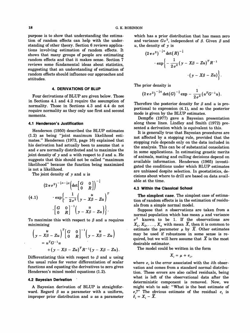
purpose is to show that understanding the estimation of random effects can help with the understanding of other theory. Section 6 reviews applications involving estimation of random effects. It shows that many groups of people are estimating random effects and that it makes sense. Section 7 reviews some fhdamental ideas about statistics, suggesting that an understanding of estimation of random effects should influence our approaches and attitudes.

4. DERIVATIONS OF BLUP

Four derivations of BLUP are given below. Those in Sections 4.1 and 4.2 require the assumption of normality. Those in Sections 4.3 and 4.4 do not require normality as they only use first and second moments.

4.1 Henderson's Justification

Henderson (1950) described the BLUP estimates (1.2) as being "joint maximum likelihood estimates." Henderson (1973, page 16) explained that his derivation had actually been to assume that u and e are normally distributed and to maximize the joint density of y and u with respect to P and u. He suggests that this should not be called "maximum likelihood" because the function being maximized is not a likelihood.

The joint density of y and u is

To maximize this with respect to p and u requires minimizing

Differentiating this with respect to P and u using the usual rules for vector differentiation of scalar functions and equating the derivatives to zero gives Henderson's mixed model equations (1.2).

4.2 Bayesian Derivation '

A Bayesian derivation of BLUP is straightforward. Regard ,tl as a. parameter with a uniform, improper prior distribution and u as a parameter

which has a prior distribution that has mean zero and variance Ga2, independent of P. Given P and u, the density of y is

( 2 7 r o ~ ) ~ ~d e t ( ~ ) - '

- Xp - Zu)TR -1

The prior density is

Therefore the posterior density for 6 and u is pro- portional to expression (4.1), and so the posterior mode is given by the BLUP estimates.

Dempfle (1977) gave a Bayesian presentation along these lines. Lindley and Smith (1972) presented a derivation which is equivalent to this.

It is generally true that Bayesian procedures are not affected by a stopping rule, provided that the stopping rule depends only on the data included in the analysis. This can be of substantial consolation in some applications. In estimating genetic merits of animals, mating and culling decisions depend on available information. Henderson (1965) investi- gated the conditions under which BLUP estimates are unbiased despite selection. In geostatistics, decisions about where to drill are based on data available at the time.

4.3 Within the Classical School

The simplest case. The simplest case of estimation of random effects is in the estimation of residuals from a simple normal model.

Suppose that n observations are taken from a normal population which has mean p and variance a 2 known to be 1. If the observations are XI, X,, . . . ,X, with mean X, then it is common to estimate the parameter p by x.Other estimates may be used if robustness in some sense is required, but we will here assume that X is the most desirable estimator.

The model could be written in the form

where ei is the error associated with the ith observation and comes from a standard normal distribution. These errors are also called residuals, being what is left of the observational data after the deterministic component is removed. Now, we might wish to ask: "What is the best estimate of e,?" The obvious estimate of the residual ei is Zi= xi- X.


Properties of the residuals as estimators of the unknown errors are the following.

1. They are linear iri the data. 2. They are unbiased in the sense that

Note however that E[e^,I e,] is nearer to zero than is ei. In some circumstances, people tend to expect 'unbiased' to be interpretable as meaning that the expectation of an estimate of a random effect given the true value of the random effect is equal to that random effect. This is not the case.

3. They have minimum mean square error amongst the class of linear unbiased estimators.

In this very simple case, none of this is very interesting or enlightening; but it is notable that there is a situation where estimation of random effects is standard practice. We need to consider situations involving more than one source of variation before anything nontrivial happens. However, it does suggest that it is reasonable to ask that estimates of random effects be linear, unbiased and minimum mean square error.

The general case. Henderson (1963) showed using Lagrange multipliers that BLUP estimates of linear combinations of fixed and random effects are the estimates that satisfy the classical require- ments of being linear, unbiased and minimum mean square error. Harville (1976) showed, fu.rther, that the Gauss-Markov theorem could be extended to cases when matrices G and R are of less than full rank. See also Ishii (1969, Example 2, pages 482-487).

A more intuitive approach to showing that the BLUP estimates have minimum mean squared error within the class of linear unbiased estimates was given by Harville (1990). First, note that

and that, as Henderson, Kempthorne, Searle and von Krosigk (1959) showed, an alternative form for the BLUP estimates is

Linear unbiased estimates of zero are of the form aTy,where a satisfies X T a = 0. They are uncorre- lated with the errors of BLUP estimates, since

E [ ( B- /3)yTa]

and

Any linear unbiased estimator of a linear combina- tion bT/3+ cTu of fixed and random effects must be of the form bTp^+ cTB + aTy, where XTa = 0. Its variance-covariance matrix of estimation errors is

~ [ { d ' ( j- 8) + c T ( s- U ) + a T y )

.{bT(p^- B ) + c T ( a- a ) + a T y j T ]

= E [ { ~ T ( B- 0)+ C ~ ( B- u ) )

- { b T ( )- /3) + cT(B- u ) l T ]+ E[aTyYTa]

+ E [ { b T ( p- 0)+ cT(B- u ) ) yTa]

+ E[aTy{bT(a -̂ 0)+ cT(B- u ) l T ]

Now E[aTyyTa1= E[aTy{ aTy)Tl is a symmetric positive semidefinite matrix, so this variance-covariance matrix of estimaiion errors exceeds that for the BLUP estimate bT/3+ cTB.

4.4 Goldberger's Derivation

Goldberger (1962) considered a linear model

y = X/3 + E ,

20 G. K. ROBINSON

where the disturbance E satisfies E(E)= 0 and V a r ( ~ )= 0. Given a new (observable) vector x, of regressors and (unobservable) prediction distur-bance E*, which is correlated with the disturbances for the data already obtained, satisfying

- E(E*)=O

E ( E , E ~ ) = wT,

Goldberger's equation (3.12) tells us that the best linear unbiased predictor of the future observation y* = x ~ O+ E* is

For our model, E = Zu + e, so

Q = (ZGZT+ R)a2.

To estimate x a + Z ~ Utake

E* = z*Tu

and hence

w T = E Z ~ Uzu+ elT] = Z ~ G Z ~ O ~ .I ( So Goldberger's derivation tells us that the best linear unbiased predictor of X ~ P+ Z ~ Uis

which is

Using the matrix identity (5.2), below, and the j second of the simultaneous equations (1.2), this is

Thus Goldberger's predictor is the same as that given by (1.2).

To the best of my knowledge, Goldberger was the first to use the term "best linear unbiased predictor" and Henderson started using the acronym BLUP in 1973.

Goldberger's derivation seems unobjectionable

from a Classical viewpoint. His emphasis is on prediction, but his formulae still apply generally to prediction of a future observation, y,, which is perfectly correlated with a past disturbance, so they do apply to estimation of random effects.

5. LINKS WITH OTHER STATISTICAL THEORY

5.1 Recovery of Inter-Block Information

Henderson, Kempthorne, Searle and von Krosigk (1959, page 196) showed that the BLUP estimate /? is identical with the generalized least-squares estimate of 0 that would be obtained after recovery of inter-block information if the random effects u were block effects. They eliminated ii from equation (1.2), giving

Now using a matrix identity which is commonly used in this subject area

gives

x T ( ~ZGZT)-~X$ x T ( ~Z G Z T ) - ' ~ .+ = + Hence

which can be seen to be the generalized least squares estimate of p, since the variance-covariance matrix of the random effects is

The matrix identity (5.1) is a particular case of

- UBVA-~U(I+ B V A - ~ u ) - ' B v A - ~

= I

of which the history and many variants, generaliza- tions and special cases are discussed by Henderson


and Searle (1981). In this paper, we will also use the matrix equality

which can be derived from (5.1). Recovery of interblock information is most com-

monly discussed for experimental data from incom- plete block designs. Recovery of the interblock information improves the efficiency of the esti-mates of the fixed effects, but the estimates based only on intra-block information are often considered to be satisfactory.

For unbalanced data, estimates of fixed effects based only on intrablock information can some-times be quite unsatisfactory. An example of this is presented below. It was discussed in Henderson, Kempthorne, Searle and von Krosigk (1959).

EXAMPLE.Fifty cows produce an average of 100 kilograms of butterfat in their first lactations. Forty of these cows survive to complete their second lactations. The average first lactation butterfat yield of these 40 cows is 110 kilograms and the average second lactation butterfat yield is 140 kilograms. Estimate the average difference between lactations in the absence of culling!

One answer is (140 - 100) kg = 40 kg, using all cows. Another answer is (140 - 110) kg = 30 kg, using only the cows which completed second lactations. This is the estimate that uses only intra-cow information. If the true correlation between first and second lactations can be taken to be 112, then recovery of inter-cow information gives the estimate 35 kg.

Intuitively, the cows culled are likely to be worse than average. Therefore the cows completing second lactations are likely to be better than average; so the first answer is likely to be too large. The cows not culled are unlikely to be as good as they appear to be because the data has been selected. An extreme case to illustrate this is that if first lactation yield and second lactation yield were uncorre- lated, then culling on first lactation would not increase average second lactation yield but it would increase the first lactation yield of cows completing a second lactation by rejecting some data. The second answer is likely to be too small because the 110 is an overestimate.

In this example, the effect of lactation parity is being regarded as a fixed effect (treatment) and cow effects are being regarded as random effects (blocks). Thinking of the BLUP estimate of the

lactation parity effect as being a Bayesian estimate, the likelihood principle tells us that the estimate does not need to be modified if culling has taken place, provided that culling decisions were based only on the data included in the analysis. Within the Classical framework, Henderson (1975) showed that selection and culling which is based on linear combinations (LTy) of the data y do not affect the optimality of the BLUP estimates provided that LTX = 8.An aspect of this formalization that I cannot understand is the meaning of selection based on the L matrix. In examples given in Henderson (1973, 1975, 1984), the numbering of the random effects is always such that best is first but ranking is not a linear function of the data. The problem has been of interest to Henderson throughout his career, but his work involving the L matrix is not widely understood or accepted.

Estimates of environmental and genetic trends from dairying data tend to suffer from biases similar to this, unless the inter-cow information is recovered. Of course, the resulting estimates are sensitive to the values used for dispersion parameters, such as the correlation in the example above, but to not recover information is equivalent to using extreme values for dispersion parameters, and is worse.

5.2 Random Effects Models

Mathematically, it is easy to see from equations (1.2) and (5.2) that when there are no fixed effects the BLUP estimates of the random effects are given by

(5.3) (ZTR-'Z + GP1)t2= ZTR-lY

and have variance-covariance matrix

In animal breeding, BLUP for random effects models is known as the selection index. See Smith (1936) and Hazel (1943). Lush (1949) referred to it as "most probable producing ability ."

Henderson (1963) describes BLUP as a form of selection index. In our notation, if @ were known, then y - X@ = Zu + e follows a random effects model, so the best estimate of u is

If we replace @ by the estimate

then the resulting estimate of u is the BLUP estimate, as shown by Henderson (1963).

22 G. K. ROBINSON

Box and Tiao (1968) presented a detailed deriva-tion of BLUP estimates for random effects models within a Bayesian framework. Dempfle (1977) gave the following Bayesian derivation, which I find intuitively helpful. The idea is due to Robertson (1955) and is only applicable when the matrix Z is of full rank.

The generalized least squares estimate of u is

and has precision

The prior estimate of u is

ii2 = 0

and has precision

The best estimate of u gives these two estimates weight in inverse proportion to their precision and is

A straightforward classical derivation is to use standard results on the multivariate normal distri-bution (e.g., Searle, 1971, page 47). Since u and y have zero means and variance-covariance matrix

the distribution of u given y has mean

and variance

in agreement with (5.3) and (5.4). This derivation shows that, when there are no fixed effects to be estimated simultaneously, the theory of estimating random effects follows the theory of correlation very closely.

Ideas about correlation are quite old. Pearson (1896, page 261) wrote

The fundamental theorems of correlation were

for the first time and almost exhaustively dis-cussed by BRAVAIS ('Analyse Mathkmatique sur les probabilitks des erreurs de situation d'un point'. MQmoires par divers Savans, T. IX., Paris, 1846, pp 255-332) nearly half a century ago. He deals with the correlation of two and three variables. . .GALTON . . . intro-duced an improved notation. . . Random effects models are also related to the

idea of regression to the mean attributed by Davis (1986) to Galton. The best estimate of a character-istic of an offspring given the characteristics of the parents is regressed towards the population mean from the parental average.

EXAMPLE.Suppose that true intelligence quo-tient (IQ) is normally distributed with mean 100 and standard deviation 15. Two tests are available. Both tests give scores that are normally distributed with mean the true IQ. The first test score has standard deviation 10 given true IQ, while the second test score has standard deviation 5. A per-son scoring 130 on the first test would be estimated to have a true IQ of 120.8 and a person scoring 130 on the second test would be estimated to have a true IQ of 127. Features of these estimates worth noting are as follows.

They are shrunk towards the overall mean (100) from the data. The amount of shrinkage is greater when the data point is less informa-tive. They are biased given true IQ. This is obvious since the raw scores are unbiased and the esti-mates are nontrivial linear functions of the raw scores. They have zero average bias when averaged over the distribution of possible true IQs. The expected value of true IQ given the data is equal to the BLUP estimate of IQ, by (5.5).

This example is far from new. In the discussion to Lindley and Smith (1972), Novick suggested that Kelley (1927) was familiar with the basic ideas of shrinkage estimators. Henderson (1973, page 15) explained that considering this example was cru-cial in his development of BLUP in 1949.

5.3 Fixed Effects Models and Admissibility

Fixed effects models are, of course, a particular case of mixed models. Stein's (1956) demonstration that the sample mean is inadmissible for the mean of a multidimensional normal population of known variance when the dimensionality is at least three has led to some theoretical work that I believe to be


of little practical value. This work is characterized by a tendency to combine unrelated estimation problems. BLUP helps us to know when to combine estimation problems. Situations where estimation problems ought to be combined are when the parameters to be estimated can be regarded as coming from some distribution. Equivalently, they are "exchangeable," or are "random effects." I agree with the view expressed by E. F. Harding in discussion of Lindley and Smith (1972) that estimates of the characteristics of butterflies in Brazil, ball bearings in Birmingham, and brussels sprouts in Belgium ought not to be related to each other.

5.4 Estimation of Variance Parameters

The estimation of variance parameters is a very extensive topic. See, for instance, Khuri and Sahai (1985). The comments below concentrate on one method of estimating variance parameters, REML, which can be interpreted as either Classical or Bayesian.

For balanced experimental data, the analysis of variance provides estimates which are often considered acceptable. Sometimes estimates of variance components are negative, in which case they are taken to be zero.

For unbalanced data, REML is the method of estimating variance components that seems to have the best credentials from a Classical viewpoint. See Robinson (1987) for a recent discussion with examples. It was expounded by Patterson and Thompson (1971). They called it "modified maximum likelihood." Some people now refer to it as "restricted maximum likelihood,"-while others use the term "residual maximum likelihood."

Thompson (1973) generalized REML to the multivariate case and showed that it may be used even when the data available has been selected in certain ways.

Consider the problem of estimating 8 for the linear model given by equation (1.1). Bayesian statisticians would, in principle, start with a joint prior distribution for 8, @ and u. If a uniform prior distribution is used for @, then the posterior mode gives a point estimate of 8 and the BLUP estimates p̂ and fi given that 8. These are not ideal estimators. Bayesian statisticians would prefer to estimate 8 by integrating over @ and u rather than merely looking at the posterior for p̂ and fi.

Harville (1974) showed that REML is equivalent to marginalizing the likelihood over the fixed effect parameters, so practical approximate Bayesian procedures for estimating dispersion parameters can use REML to approximately integrate over the fixed and random el'ects.

The Classical concept of modified profile likelihood due to Barndorff-Nielsen (1983) can also be regarded as an approximate Bayesian technique in which second derivatives of the posterior density are used to approximately integrate out nuisance parameters by assuming normal distributions with the given second derivatives for the nuisance parameters. Such approximate integration gives a multiplicative factor that is the exponential of the - power of the determinant of the observed information matrix for the nuisance parameters.

5.5 Estimation of Outliers

When fitting models with only one variance component, it is common practice to compute residuals in order to look for outliers. If it appears that some data points are outliers, then they may be ignored in some circumstances, they may be highlighted in other circumstances, or appropriately robust methods of analysis may be used for estimating parameters of interest.

When fitting models with two or more variance components, BLUP estimates of the realized values of random effects are the natural generalization of the concept of residuals. Outlying values of some random effects will mean that groups of data points are likely to fail to fit the model, but looking at the estimates of the random effects provides a more sensitive test for such outliers than merely looking at residuals. Fellner (1986) discusses this topic with some examples.

5.6 Estimation of Fixed and Random Effects when the Dispersion Parameters Must be Estimated

For most of this paper, estimation of random effects is considered under the assumption that 8 is known. All approaches seem to agree as to the best estimates of random effects in this case. There is less consensus about what to do when 8 must be estimated from the data.

Student's t-test differs from simple use of the normal distribution in that it takes the uncertainty of estimating the variance of a normal distribution into account when considering hypotheses about the mean. It is natural to suspect that BLUP estimates or their estimated precision would need to be modified when 8 must be estimated.

Kackar and Harville (1981) showed that estimates p̂ and fi remain unbiased when 8 must be estimated provided that the estimates of components of 8 are translation-invariant and are even functions of the data vector. This suggests that the BLUP point estimates will generally not need to be modified. We do in principle, however, need to modify the estimated precision of the BLUP esti-

24 G.K. ROBINSON

mates. In practice, this difficulty is sometimes ignored or handled by conservative interpretation of calculations based on the best point estimate of the dispersion parameters.

Estimating the precision of BLUP estimates using the Classical approach seems mathematically complicated when the uncertainty in dispersion parameters is considered. For some recent work on the topic, see Kackar and Harville (1984), Harville (1985), Prasad and Rao (1986), Fuller and Harter (1987) and Jeske and Harville (1988).

From a Bayesian point of view, the estimation of dispersion parameters taking the uncertainty in the fixed and random effects into account and the estimation of fixed and random effects taking uncertainty in the dispersion parameters into account are not different in principle, but different types of approximation are likely to be appropriate. A prac-tical approximate Bayesian procedure for estimating the precision of fixed and random effects is to approximate the Bayesian posterior distribution for 8 by a discrete distribution over a small number of possibilities and to use BLUP at each of these possibilities thereby calculating a mixture of distributions as posterior for the fixed and random effects.

5.7 Empirical Bayes Methods

Empirical Bayes methods are concerned first with estimating distributions from which random effects have been generated. Once a distribution of random effects has been estimated, this distribution is used to estimate realized values of random effects using Bayes' Theorem. If the distribution of random effects is Gaussian, then empirical Bayes methods would use BLUP estimates to estimate fixed and random effects.

When parametric assumptions are made about the distribution of the random effects then the statistical methods employed are described as parametric empirical Bayes. BLUP is equivalent to one of the techniques of parametric empirical Bayes methodology.

5.8 Ranking and Selection

BLUP was originally developed for ranking and selection in the contexts of animal breeding and genetics. It is an appropriate technique when the ideal ranking or selection criteria involve unobservable characteristics that may be regarded as random effects.

Much theoretical work on ranking and selection seems to have been done in ignorance of BLUP. This work tries to control the probability that ranking or selection decisions will be made correctly,

when the probability is to be calculated before the data are available. In contrast, BLUP is concerned with correct selection between random effects given the data, as in Berger and Deely (1988).

Stein (1945) presented a procedure that obtains an interval estimate of preassigned length for the mean of a normal distribution when the population variance is unknown. It achieves this by sampling in two stages and ignoring the information about the population variance contained in the sample variance for the second sample. It is not a satisfactory technique for practical application because it concentrates on initial precision rather than final precision, it does not achieve its nominal coverage probability conditional on the ancillary statistic s,2/s,2 where s8 is the sample variance in the ith stage of sampling, and it violates the likelihood principle. Stein's procedure is a foundation stone for some theoretical work on ranking and selection that I believe to be misguided. BLUP would be a better foundation stone.

6. APPLICATIONS

There are a number of situations in which estimation of random effects is precisely what is required. Morris (1983) has discussed several of them. A brief discussion of some of them should help to establish the point that estimation of random effects is a legitimate activity, even if not very common.

There are four features which are common to most of the applications.

1. The data and the random effects to be estimated are often multivariate.

2. Computational issues are often extremely important.

3. Sparsity or approximate sparsity of partial correlation matrices is more important than sparsity or approximate sparsity of correlation matrices.

4. Random effects selected on the basis of the estimates made are often of particular interest.

People having difficulty with one of these features for any of the applications should consider how the feature is handled for the other applications.

6.1 Estimation of Merit of Individuals

Efron and Morris (1977) discussed estimating the batting abilities of 18 baseball players. The true batting abilities can be regarded as random effects drawn from a distribution. To estimate the mean and variance of the distribution of batting abilities

THE ESTIMATION OF RANDOM EFFECTS

is of some interest, but the main problem is estimating the random effects.

In plant variety trials, it is sometimes realistic to regard the varieties as random effects since they have been generated by processes that are random at the chromosome level. The objective of variety trials is generally to find the best varieties or to estimate the yield (or some other characteristic) of all varieties, not to estimate the parameters of the distribution from which the varieties are a sample.

6.2 Selection Index

In quantitative genetics, the selection index provides a way of ranking plants or animals given measurements on several traits on the individuals to be ranked and their relatives.

The selection index can be seen to be a particular case of the BLUP estimates of random effects

using (5.2). The model being fitted is

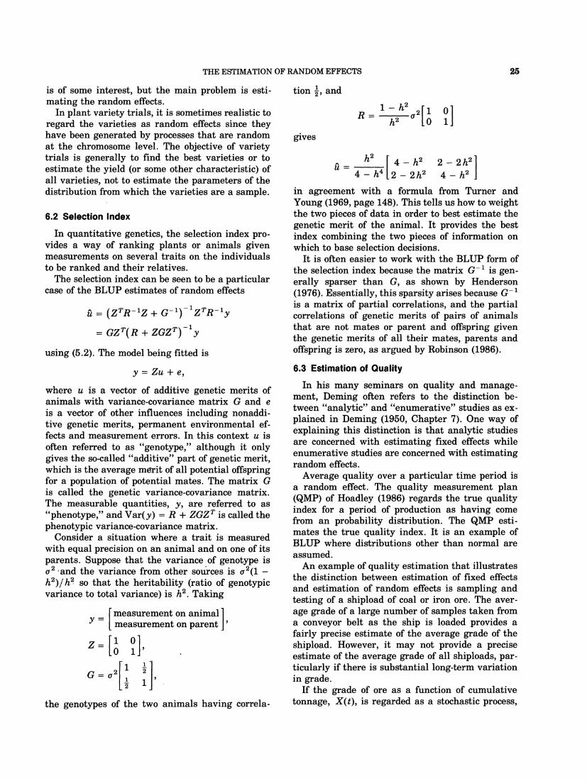
where u is a vector of additive genetic merits of animals with variance-covariance matrix G and e is a vector of other influences including nonaddi- tive genetic merits, permanent environmental effects and measurement errors. In this context u is often referred to as "genotype," although it only gives the so-called "additive" part of genetic merit, which is the average merit of all potential offspring for a population of potential mates. The matrix G is called the genetic variance-covariance matrix. The measurable quantities, y, are referred to as "phenotype," and Var(y) = R + ZGZT is called the phenotypic variance-covariance matrix.

Consider a situation where a trait is measured with equal precision on an animal and on one of its parents. Suppose that the variance of genotype is u 2 ,and the variance from other sources is u2(1 -h2)/h2 SO that the heritability (ratio of genotypic variance to total variance) is h2.Taking

measurement on animal Y = [ measurement on parent 'I z = [; i], G = ..[;t],

tion 9 , and

gives

in agreement with a formula from Turner and Young (1969, page 148). This tells us how to weight the two pieces of data in order to best estimate the genetic merit of the animal. It provides the best index combining the two pieces of information on which to base selection decisions.

It is often easier to work with the BLUP form of the selection index because the matrix G-' is generally sparser than G, as shown by Henderson (1976). Essentially, this sparsity arises because G-I is a matrix of partial correlations, and the partial correlations of genetic merits of pairs of animals that are not mates or parent and offspring given the genetic merits of all their mates, parents and offspring is zero, as argued by Robinson (1986).

6.3 Estimation of Quality

In his many seminars on quality and manage- ment, Deming often refers to the distinction between "analytic" and "enumerative" studies as explained in Deming (1950, Chapter 7). One way of explaining this distinction is that analytic studies are concerned with estimating fixed effects while enumerative studies are concerned with estimating random effects.

Average quality over a particular time period is a random effect. The quality measurement plan (QMP) of Hoadley (1986) regards the true quality index for a period of production as having come from an probability distribution. The QMP estimates the true quality index. It is an example of BLUP where distributions other than normal are assumed.

An example of quality estimation that illustrates the distinction between estimation of fixed effects and estimation of random effects is sampling and testing of a shipload of coal or iron ore. The average grade of a large number of samples taken from a conveyor belt as the ship is loaded provides a fairly precise estimate of the average grade of the shipload. However, it may not provide a precise estimate of the average grade of all shiploads, par- ticularly if there is substantial long-term variation in grade.

If the grade of ore as a function of cumulative the genotypes of the two animals having correla- tonnage, X ( t ) , is regarded as a stochastic process,

then the average grade of the shipload is a random effect. It is jf X(t) dt/(B - A) for some constants A and B that delimit the shipload. The average grade of all shiploads is a fixed effect. It is the mean of a stochastic process.

Deming would regard the sampling and testing as being an "analytic" study insofar as it is studying the mean of all shiploads and as being an "enumerative" study in so far as it is studying a single shipload.

Further details of this application appear in Saunders, Robinson, Lwin and Holmes (1989). See also Cochran (1946), Yates (1949), Jowett (1952), Duncan (1962), Matheron (1965) and Gy (1982).

It should be noted that many sampling standards are designed to estimate the population mean of a process (an analytic study-a fixed effect), not the mean of a lot (an enumerative study-a random effect), but they fail to make the distinction clear. Often, the mean of a lot can be estimated much more precisely than the process mean with given data.

6.4 Time Series and Kalman Filtering

Some time series problems are concerned with estimating fixed parameters associated with time series. Many other time series problems may use- fully be regarded as problems of estimating random effects.

The observed value of a time series is the sum of signal and noise that may be regarded as random effects that differ in their spectra. Smoothing, filtering and prediction problems all involve estimation of the random effects that form the signal.

To illustrate the link between estimation of random effects and time series, we consider the Kalman filter, which is used for estimating the current value of the signal in a time series. The estimates obtained by Kalman filtering and by BLUP must be the same because of their optimality properties. However, it seems worthwhile to consider an approach to Kalman filtering directly from ' BLUP. See also Broemeling and Diaz (1985), Harrison and Stevens (1976) and Sallas and Harville (1981). Inci- dentally, Sorenson (1970) suggests that the Kalman filter is not entirely due to Kalman.

We follow the terminology of Meinhold and Singpurwalla (1983) who explained the Kalman filter in a Bayesian framework.

Suppose that unobservable vector-valued random variables u, are related by

for t = 1,2, . . . , n with u, = 0. An observable vec-

tor-valued random variable y, is related to the u, by

yt = F,u, + v,.

Assume that G, and F, are known. Further, suppose that the w, and v, are independent and normally distributed with zero means and known variances W, and V,.

This is an example of a random effects model. The variance-covariance matrix for the random effects is not simple. Denoting it by

where

it is defined recursively by the following equations:

g11 = Wl g . .= for i > j

LJ

g . .IJ = g . .LJ-1GT for i < jJ

g . . = G.g.1 1 1 - l i + Wi

= gii-l ~ ' ?+ Wi.

The matrix G-l is simpler than G. It is block tridiagonal essentially because the partial correlations of pairs of nonadjacent u, given an intermedi- ate u, are always zero. It is

where

g n n= W,-:l,

for i < n,

and all other g i J are zero matrices. The matrix algebra required to show equivalence

of BLUP estimates with the Kalman-Bucy algorithm is not trivial, but the statistical theory is simple. The Kalman-Bucy algorithm is computa- tionally efficient because computations for time t make use of results obtained for time t - 1. This use of the immediate past depends crucially on the simplicity of the matrix G-l, which is due to the Markovian nature of the process generating the u,. A general principle illustrated here is that partial correlation matrices are more important computa- tionally than correlation matrices.

Note that, being equivalent to BLUP estimation


of random effects, Kalman filtering is not maxi- ferent numbers of employees and different safety mum likelihood. records. This example was discussed by Mswbray

(1914). 6.5 Removing Noise froin Images In terminology like that of the present paper, let

Besag (1986) reviewed many methods of attempt- ing to restore images that have been corrupted by noise. The simplest models for continuously variable intensity over a grid are auto-normal models in which the point intensities are normally distributed and have nonzero partial correlations with intensities at neighboring points on the grid. Within our framework, the true image is a random effect that we wish to estimate. What Besag calls the "maximum a posteriori" estimate of the true image is equivalent to BLUP for these models.

As in other applications being discussed, the objective of primary interest is to estimate random effects.

6.6 Geostatistics

The method of geological reserve estimation known as Kriging is essentially the same as BLUP. It was developed independently from BLUP. A difference from the estimation of genetic merits is that variance parameters are estimated more fre- quently than in genetic applications.

The random effect that is estimated is the pattern of grade of ore as a function of position in two- or three-dimensional space. Estimation of the random effect is of much more immediate interest to a company that is considering a mining operation than is estimation of the parameters of the distribution from which the pattern of grade is a sample.

There is much more to ore reserve estimation than Kriging. A concise summary of some of the difficulties written by Matheron appears in the Foreword to Journel and Huijbregts (1978). One very substantial difficulty is that the economic fea- sibility of mining a deposit is based on a small number of drill-holes, but decisions about which blocks of ore will be processed and which will be dumped as waste will be made using data from blast-holes that are much more numerous than the drill-holes. The average grade of the ore that will be selected for processing is much harder to predict than is the overall average grade. This difficulty is most acute when only a small proportion of the rock to be mined will be processed.

6.7 Credibility Theory

Credibility theory is a coll6ction of ideas used by actuaries to work out insurance premiums. As an example, consider setting workers' compensation premiums for industrial companies that have dif-

uidenote the true fair premium for company number i. The uimay be regarded as random effects and the BLUP estimates of them will be useful. If a company has an extensive claims record, then its estimated premium will depend almost entirely on its own record. If a company has little claims record, then the estimated premium for that company will differ little from the average premium for all companies.

The classical approach to credibility is to assume that there is a credibility factor, denoted Z(t), where t is the size of the risk class, such that the estimated fair premium is

where y is the fair premium as estimated using data for the single risk class only, and m' is the average fair premium over all risk classes. The function Z(t) is chosen in a somewhat arbitrary manner which need not concern us here. (See Hick- man, 1975.)

The Bayesian approach to credibility is to use conjugate prior distributions for the ui.The development of the Bayesian approach is attributed to Bailey (1945,1950) and Mayerson (1965). See Kahn (1982) for a brief review.

6.8 Small-Area Estimation

Small-area estimation involves using direct survey information from areas of individual interest together with information on similar or related areas. It has been found that more precise estimates can be made than if information on the other areas had been ignored. One approach is to regard the quantities of interest in the individual areas as .being random effects which are to be estimated. See Battese, Harter and Fuller (1988), Prasad and Rao (1986), Fuller and Harter (1987) and the other papers in the same volume from the May 1985 International Symposium on Small Area Statistics for further information about this field of application.

7. DISCUSSION

7.1 Prediction or Estimation?

Henderson originally used the term "predictor" rather than "estimator" in order to evade criticism of BLUP. Henderson (1984, page 37) expressed

28 G. K. ROBINSON

doubts about the appropriateness of the terminol- 7.3 Fixed and Random Effects ogy:

Which is the more-logical concept, prediction of a random variable or estimation of the realized value of a random variable? If we have an animal already born, it seems reasonable to describe the evaluation of its breeding value as an estimation problem. On the other hand, if we are interested in evaluating the potential breeding value of a mating between two poten-tial parents, this would be a problem in predic-tion. If we are interested in future records, the problem is clearly one of prediction.

From conversations with him, I believe that he accepts the weaknesses of the terminology:

in some applications, the thing being esti-mated has already occurred, and BLUP is a predictor only in the same way as most estimates are predictors-if they were not relevant to something which might happen in the future then they would not be of interest.

It has become common practice to "estimate" fixed effects and to "predict" random effects. I believe that Henderson would be content to use terms such as "estimate" and "estimate of realized value." I prefer simple terminology-to use "estimation" of both fixed and random effects.

7.2 Unbiasedness and Shrinkage

The BLUP estimator ii of u is sometimes said to be "unbiased" because it satisfies

~ [ i i ]= E [ u ] .

It is also described as a "shrinkage" estimator because its components are less spread than the generalized least-squares estimates that would be used if the components of u were regarded as fixed effects. These two descriptions seem to be in con-flict with one another.

The difficulty is that the use of the term "unbi-,asedY'is very different from the condition

E [ E i ) u ] = u foral lu ,

which is what many people intuitively expect, par-ticularly in circumstances where the random pro-cesses generating the random effects (genetic mer-its of dairy bulls or ore grades in a deposit, for instance) occur prior to other processes generating noise in the data. Whenever I mean "unbiased" in the sense that E[iil = E[ul I try to make this very clear. Perhaps some new terminology would be a good idea.

Eisenhart (1947) distinguished between two uses for analysis of variance: (1) detection and estima-tion of fixed (constant) relations among the means of subsets of the universe of objects concerned; and (2) detection and estimation of components of (ran-dom) variation associated with a composite popula-tion. He suggested two parallel sets of questions to help distinguish fixed and random effects, and these tend to imply that estimation of random effects is not sensible because effects of interest must be treated as fixed.

1. "Are the conclusions to be confined to the things actually studied (the animals, or the plots); to the immediate sources of these things (the herds, or the fields); or expanded to apply to more general populations (the species, or the farmland of the state)?"

2. "In complete repetitions of the experiment would the same things be studied again (the same animals, or the same plots); would new samples be drawn from the identical sources (new samples of animal from the same herds, or new experimental arrangements on the same fields); or would new samples be drawn from more general populations (new samples of animals from new herds, or new experimen-tal arrangements on new fields)?"

The discussion of the difference between fixed and random effects given in Searle (1971) is simi-larly misleading in my view. On page 383, Searle writes

. . .when inferences are going to be confined to the effects in the model the effects are consid-ered fixed; and when inferences will be made about a population of effects from which those in the data are considered to be a random sample then the effects are considered as ran-dom.

Both of these people have defined their terms in such a way that estimation of random effects is not possible.

In my view, there are two questions which might need to be answered in order to decide whether the effects in a class are to be treated as fixed or random. The first of these is: Do these effects come from a probability distribution? If the effects do not come from a probability distribution then the ef-fects should be treated as fixed.

If the effects do come from a probability distribu-tion, then if the effects are themselves being esti-mated they should be treated as random. For classes

- -


of effects which are nuisance parameters, there is a second question to be answered: Is interclass information to be recovered for this class of effects? If interclass information is to be recovered then treat the class of effects as random, otherwise fixed.

EXAMPLE.When estimating the genetic merit of dairy bulls, the herd-year-season effects that are used to model environmental variation do come from a probability distribution which describes variation: that between herds, years and calving seasons. When estimating herd-year-season effects I believe that they should be treated as random. However, when estimating genetic merits of dairy bulls I believe that herd-year-season effects should be treated as fixed because the inter-herd information should not be recovered-Farmers' choices of artificial insemination bulls and their choice of feeding regimes are somewhat related, and to recover the inter-herd information woulh favor the bulls that were more often chosen by farmers providing high feed intakes. Similarly, bull choices vary between years, and yearly climatic variation might bias estimated breeding values. The decision not to recover inter-herd-year-season information is based on a willingness to sacrifice some efficiency for greater robustness relative to departures from the assumptions of the model.

I agree with Tukey's remark made in discussion of Nelder (1977): " . . .our focus must be on questions, not models." The choice of whether a class of effects is to treated as fixed or random may vary with the question which we are trying to answer.

7.4 Generalizing Likelihood

When Fisher (1922, page 326) introduced the idea of likelihood as the probability of data given a hypothesis regarded as a function of the hypothesis, I doubt that he had considered problems of estimating random effects.

For estimation of fixed effects and dispersion parameters for the random effects model (1.1) the usual definition of likelihood seems adequate. How- ever, if we wish to estimate the random effects, u , then the usual concept of likelihood seems to oblige us to regard the value of u as part of the hypothesis. In effect, the idea of likelihood tends to force us to regard things that we wish to estimate as fixed rather than random effects.

In my view, when we specify a mixed model the dispersion of the random effects, u, and the dispersion of the error, e, ought to be given similar logical status. How can this be achieved?

One possible attempt to resolve the problem based on Bayesian concepts would be to regard the as-

sumed distribution of the random effects as an objective prior distribution. It is different in logical status from a subjective prior distribution from which the fixed effects might be considered to have come. One distinguishing feature is that the objec-tive distribution of the random effects is being used to describe variation while the subjective prior distribution of the fixed effects is being used to describe uncertainty. A second distinguishing feature is that assumptions about the distribution of the random effects can be tested.

To use such an objective prior distribution for random effects should not be considered to make one a Bayesian. Good (1965, page 8) wrote

the essential defining property of a Bayesian is that he regards it as meaningful to talk about the probability P(H I E) of hypothesis H, given evidence E.

To be a Bayesian, you would need to be willing to put a prior distribution on fixed effects as well as random effects. Kempthorne in the discussion of Lindley and Smith (1972, p-age 37) described people who wish to estimate random effects as "legiti-mate" Bayesians; I agree with the ideas behind this designation, but I prefer to adhere to Good's use of the term "Bayesian."

This attempt to define likelihood in a way which allows estimation of random effects separates the distribution of e (the likelihood), the distribution of u (the objective prior distribution), and the uncertainty about 0 and 0 (the subjective prior distribution for Bayesians) into three separate boxes. It does not achieve the stated goal of giving similar logical status to the dispersion of e and the dispersion of u.

Most likely unobservables. An alternative resolution of the problem based on Classical concepts is to formalize the principle behind Henderson's derivation of BLUP. This principle does achieve the goal of giving similar logical status to the dispersion of e and the dispersion of u. A colleague, T. Lwin, and I would like to suggest the name method of most likely unobservables for it.

Given the mixed model (1.1) and having observed the data y, the method of most likely unobservables is to say that the best estimates of 0, u and e are the ones that maximize the density of the unobservable~u and e subject to the constraint (1.1) of having observed the data. Because there are n constraints and n components to the vector e, the easiest way to solve for the maximum is to set

and maximize the joint density of u and e with

30 G. K. ROBINSON

respect to /3 and u. This is precisely Henderson's derivation of BLUP discussed in Section 4.1.

For a fixed effects model, the likelihood of the data and the likelihood of the errors are equal, so the method of most likely unobservables gives estimates of the fixed effects that are the maximum likelihood estimates and gives estimates of the errors, e, that are the usual residuals.

7.5 On Schools of Thought

I believe that the distinction between fixed and random effects should be clarified before differences between schools of thought are considered.

Statistics is concerned with both variation and uncertainty. Classical statistics can be distin-guished from Bayesian statistics by its refusal to use probability distributions to describe uncer-tainty. However, it is quite willing to use probability distributions to describe variation, and this should include variation between random effects. Once this is clarified, several situations in which the two schools of thought appeared to give different answers instead demonstrate close agreement between the schools.

There are a number of reasons why the estimation of random effects has been neglected to some extent by the Classical (Neyman-Pearson-Wald, Berkeley) school of thought.

1. The distinction between fixed and random effects has been often taken to be that effects are random when you are not interested in their individual values. Searle (1971), for instance, seems to suggest this. This implies that you should never be interested in estimating random effects.

2. The idea of estimating random effects seems suspiciously Bayesian to some Classical statisticians. The gulf between Bayesian and Clas- sical statisticians seems to be like many other gulfs between schools of thought in that the adherents of each school emphasize the differences between schools rather than the similar- ities.

Within the Bayesian paradigm, there is little reason for distinguishing between fixed and random effects. All effects are treated as random in the sense that probability distributions used to describe uncertainty are not treated any differently from probability distributions used to describe variation.

ACKNOWLEDGMENT

I am thankful for the helpful criticism provided by the editors, C. N. Morris and the late M. H. DeGroot, two referees; colleagues too numerous to

list individually-colleagues from the Herd Im- provement Section of the Victorian Department of Agriculture, the Animal Genetics and Breeding Unit of the University of New England, and the Division of Mathematics and Statistics of the Commonwealth Scientific and Industrial Research Organization-and many other people with whom I have discussed these issues.

REFERENCES

BAILEY,A. L. (1945).A generalized theory of credibility. Pro- ceedings of the Casualty Actuarial Society 32.

BAILEY,A. L. (1950).Credibility procedures. Proceedings of the Casualty Actuarial Society 37.

BARNDORFF-NIELSEN,0. (1983).On a formula for the distribution of the maximum likelihood estimator. Biometrika 70 343-365.

BATTESE,G. E., HARTER, R. M. and FULLER, W. A. (1988).An error-components model for prediction of county crop areas using survey and satellite data. J. Amer. Statist. Assoc. 83 28-36.

BERGER,J . 0 . and DEELY, J. (1988).A Bayesian approach to ranking and selection of related means with alternatives to analysis-of-variance methodology. J. Amer. Statist. Assoc. 83 364-373.

BESAG,J. (1986).On the statistical analysis of dirty pictures (with discussion). J. Roy. Statist. Soc. Ser. B 48 259-302.

Box, G. E.P. and l h o , G. C. (1968).Bayesian estimation of means for the random effects model. J. Amer. Statist. Assoc. 63 174-181.

BROEMELING, A. and DMZ, J . (1985).Some Bayesian L., YUSOFF, solutions for problems of adaptive estimation in linear dy- namic systems. Comm. Statist. Theory Methods 14 401-418.

COCHRAN,W. G. (1946).The relative accuracy of systematic and stratified random samples from a certain class of populations. Ann. Math. Statist. 17 164-177.

DAVIS, C. E. (1986).Regression to the mean. In Encyclopedia of Statistical Sciences 7 706-708.Wiley, New York.

DAWID,A. P. (1976).Comment on "Plausibility inference" by 0 . Barndorff-Nielsen. J . Roy. Statist. Soc. Ser. B 38 123-125.

DEMWG,W. E. (1950).Some Theory of Sampling. Wiley, New York.

DEMPFLE,L. (1977).Comparison of several sire evaluation methods in dairy cattle breeding. Livestock Production Science 4 129-139.

DUNCAN,A. J . (1962).Bulk sampling: Problems and lines of attack. Technometrics 4 319-344.

EFRON, B. and MORRIS, C. (1977).Stein's paradox in statistics. Scientific Amer. 236 (5) 119- 127.

EISENHART,C. (1947).The assumptions underlying the analysis of variance. Biometrics 3 1-21.

FAY, R. E. and HERRIOT, R. A. (1979).Estimates of income for small places: An application of James-Stein procedures to census data. J. Amer. Statist. Assoc. 74 269-277.

FELLNER,W. H. (1986).Robust estimation of variance components. Technometrics 28 51-60.

FISHER, R. A. (1922).On the mathematical foundations of theoretical statistics. Philos. Trans. Roy. Soc. London Ser. A 222 309-368.

FULLER, W. A. and HARTER, R. M. (1987). The multivariate components of variance model for small area estimation. In Small Area Statistics (R. Platek, J. N. K. Rao, C. E. Sarn- dal and M. P. Singh, eds.) 103-123.Wiley, New York.


GOLDBERGER,A. S. (1962). Best linear unbiased prediction in the generalized linear regression model. J . Amer. Statist. Assoc. 57 369-375. -

GOOD, I. J. (1965). The Estimation of Probabilities. MIT Press, Cambridge, Mass.

GY, P. (1982). Sampling of Particulate Materials. North-Holland, Amsterdani.

HARRISON, C. F. (1976). Bayesian forecasting P. J. and STEVENS, (with discussion). J. Roy. Statist. Soc. Ser. B 38 205-247.

HARVILLE,D. A. (1974). Bayesian inference for variance components using only error contrasts. Biometrika 61 383-385.

HARVILLE,D. A. (1976). Extension of the Gauss-Markov theorem to include the estimation of random effects. Ann. Statist. 4 384-395.

HARVILLE,D. A. (1984). Discussion of papers by Wahba, Journel and Henderson. In Statistics: An Appraisal. Proceedings 50th Anniversary Conference Iowa State Statistical Labora- tory (H. A. David and H. T. David, eds.) 281-286. Iowa State Univ. Press, Ames, Ia.

HARVILLE,D. A. (1985). Decomposition of prediction error. J. Amer. Statist. Assoc. 80 132-138.

HARVILLE,D. A. (1990). BLUP (Best Linear Unbiased Predic- tion) and Beyond. In Advances in Statistical Methods for Genetic Improvement of Livestock (D. Gianola and K. Ham- mond, eds.) 239-276. Springer, New York.

HAZEL,L. N. (1943). The genetic basis for constructing selection indexes. Genetics 28 476-490.

HENDERSON, (1950). Estimation of genetic parameters C. R. (abstract). Ann. Math. Statist. 21 309-310.

HENDERSON,C. R. (1963). Selection index and expected genetic advance. In Statistical Genetics and Plant Breeding 141-163. Nat. Acad. Sci., Nat. Res. Council, Publication 982, Washington, DC.

HENDERSON,C. R. (1965). A method of determining if selection will bias estimates. J. Animal Sci. 24 849.

HENDERSON,C. R. (1973). Sire evaluation and genetic trends. In Proceedings of the Animal Breeding and Genetics Sympo- sium in Honour of Dr. Jay L. Lush 10-41. Amer. Soc. Animal Sci. -Amer. Dairy Sci. Assn. -Poultry Sci. Assn., Champaign, Ill.

HENDERSON, linear unbiased estimation and C. R. (1975a). ~ e s t prediction under a selection model. Biometrics 31 423-447.

HENDERSON,C. R. (1976). A simple method for computing the inverse of a numerator relationship matrix used in prediction of breeding values. Biometrics 32 69-83.

HENDERSON,C. R. (1984). Applications of Linear Models in Animal Breeding. University of Guelph.

HENDERSON, O., SEARLE, C. R., KEMFTHORNE, S. R. and VON

KROSIGK,C. N. (1959). Estimation of environmental and genetic trends from records subject to culling. Biometrics 13 192-218.

HENDERSON, H. V. and SEARLE, S. R. (1981). On deriving the inverse of a sum of matrices. SZAM Rev. 23 53-60.

HICKMAN,J. C. (1975). Introduction and historical overview of credibility. In Credibility Theory and Applications (P. M. Kahn, ed.) 181-192. Academic, New York.

HOADLEY,B. (1986). Quality Measurement Plan (QMP). In En- cyclopedia of Statistical Sciences 7 373-398. Wiley, New York.

ISHII, G. (1969). Optimality of unbiased predictors. Ann. Inst. Statist. Math. 21 471-488.

JESKE, D. R. and HARVILLE, D. A. (1988). Prediction-interval procedures and (fixed-effects) confidence-interval procedures for mixed linear models. Comm. Statist. Theory Methods 17 1053-1087.

JOURNEL,A. G. and HUIJBREGTS, CH. J. (1978). Mining Geo- statistics. Academic, New York.

JOWE'IT, G. H. (1952). The accuracy of systematic sampling from conveyor belts. J. Roy. Statist. Soc. Ser. C 150-59.

KACKAR,R. N. and HARVILLE, D. A. (1981). Unbiasedness of two-stage estimation and prediction procedures for mixed linear models. Comm. Statist. A-Theory Methods 10 1249-1261.

KACKAR,R. N. and HARVILLE, D. A. (1984). Approximations for standard errors of estimators of fixed and random effects in mixed linear models. J. Amer. Statist. Assoc. 79 853-862.

KAHN, P. M. (1982). Credibility. In Encyclopedia of Statistical Science 2 222-224. Wiley, New York.

KELLEY,T. L. (1927). The Interpretation of Educational Mea- surements. World Books, New York.

KHURI, A. I. and SAHAI, H. (1985). Variance components analysis: A selective literature survey. Internat. Statist. Rev. 53 279-300.

LINDLEYD. V. and SMITH, A. F. M. (1972). Bayes estimates for the linear model (with discussion). J. Roy. Statist. Soc. Ser. B 34 1-41.

LUSH,J. L. (1949). Animal Breeding Plans, 3rd ed. Iowa State College Press, Ames, Ia.

MATHERON,G. (1965). Les Variables Regionalise'es et Leur Ap- plication. Masson, Paris.

MAYERSON,A. L. (1965). A Bayesian view of credibility. Pro- ceedings of the Casualty Actuarial Society 51.

MEINHOLD, N. D. (1983). Understand- R. J. and SINGPURWALLA, ing the Kalman filter. Amer. Statist. 37 123-127.

MORRIS, C. N. (1983). Parametric empirical Bayes inference: Theory and applications. J. Amer. Statist. Assoc. 78 47-55.

MOWBRAY,A. H. (1914). How extensive a payroll exposure is necessary to give a dependable pure premium? Proceedings of the Casualty Actuarial Society 1.

NELDER,J. A. (1977). A reformulation of linear models (with discussion). J . Roy. Statist. Soc. Ser. A 140 48-76.

PATTERSON,H. D. and THOMPSON, R. (1971). Recovery of interblock information w h m block sizes are unequal. Biometrika 58 545-554.

PEARSON,K. (1896). Mathematical contributions to the theory of evolution. 111. Regression, heredity and panmixia. Philos. Trans. Roy. Soc. London Ser. A 187 253-318.

PRASAD,N. G. N. and RAO, J. N. K. (1986). On the estimation of mean square error of small area estimators. 1986 Proceed-ings of the Section on Survey Research Methods, American Statistical Association 108-116.

ROBERTSON,A. (1955). Prediction equations in quantitative ge- . netics. Biometrics 1195-98. ROBINSON,D. L. (1987). Estimation and use of variance compo-

nents. The Statistician 36 3-14. ROBINSON,G. K. (1986). Group effects and computing strategies

for models for estimating breeding values. J . Dairy Sci. 69 3106-3111.

ROBINSON,G. K. and JONES, L. P. (1987). Approximations for prediction error variances. J. Dairy Sci. 70 1623-1632.

SALLAS,W. M. and HARVILLE, D. A. (1981). Best linear recursive estimation for mixed linear models. J. Amer. Statist. As- SOC. 76 860-869.

SAUNDERS, G. K., LWIN, T. and HOLMES, I. W., ROBINSON, R. J. (1989). A simplified variogram method for determining the estimation error variance in sampling from a continuous stream. Internat. J. Mineral Processing 25 175-198.

SEARLE,S. R. (1971). Linear Models. Wiley, New York. SMITH,H. F. (1936). A discriminant function for plarit selection.

Ann. Eugenics 7 240-250.

32 G. K. ROBINSON

SORENSON,H. W. (1970). Least-squares estimation from Gauss to Kalman. ZEEE Spectrum 7 63-68.

STEIN, C. (1945). A two-sample test for a linear hypothesis whose power is independent of the variance. Ann. Math. Statist. 16 243-258.

STEIN, C. (1956). Inadmissibility of the usual estimator for the mean of a multivariate normal distribution. Proc. Third Berkeley Symp. Math. Statist. Probab. 1197-206. Univ. California Press, Berkeley.

Comment Katherine Campbell

It has been a pleasure to read about the long history of Best Linear Unbiased Prediction, and especially about its uses in traditional statistical areas of application such as agriculture. My own experience with BLUP is in the context of ill-posed inverse problems, and I would like to discuss this paper from this point of view, where the random effects are generated by hypothesized superpopula- tions, in contrast with the identifiable populations considered by Robinson.

MODEL-BASED ESTIMATION FOR ILL-POSED INVERSE PROBLEMS

The author mentions two examples of superpopulation approaches to estimation: image restoration and neostatistics. The same ideas are also used in model-based estimation for finite populations, function approximation and many other inference problems. These problems concern inference about a reality that is in principle completely determined, but whose observation is limited by the number and/or resolution of the feasible measurements, as well as by noise. In geophysics, x-ray imaging and many other areas of science and engineering these are known as inverse problems (O'Sullivan, 1986; Tarantola, 1987).

The unknown reality we may consider to be a function m defined oi some domain T. The data typically consist of noisy observations on a finite number n of functionals of m. We can write the data vector y in terms of a transformation L map- ping m into an n-dimensional vector:

Katherine Campbell is a staff member of the Statis- tics Group, Los Alamos National Laboratory, Los Alamos, New Mexico 87545.

THOMPSON,R. (1973). The estimation of variance and covariance components with an application when records are subject to culling. Biometries 39 527-550.

TURNER,H. N. and YOUNG, S. S. Y. (1973). Quantitative Genet- ics in Sheep Breeding. Macmillan. New York.

YATES,F. (1949). Systematic sampling. Philos. Trans. Roy. Soc. London Ser. A 241 345-377.

In the sequel, we will assume that L is a linear transformation, i.e., that the observed functionals are linear. In particular, if the cardinality 1 T ) of T is finite, L can be represented by an n x IT ( matrix.

BLUP arises when we embed this problem in a superpopulation model, under which m is one realization (albeit the only one of interest) of a stochastic process M indexed by T. This superpopulation model has two components, corresponding to the "fixed" and "random" effects in Robinson's discussion. The fixed effects define the mean of the superpopulation, which is here assumed to lie in a finite- dimensional subspace of functions on T. We denote this subspace by R(F), the range of the linear operator F that maps a p-vector b into the function

Fb = x bifi.

where {f,, . . . ,f,) is a basis for the subspace. Any realization of M can then be written as a

sum F/3 + u, where /3 is an unknown vector of p fixed effects and u is a realization of a stochastic "random effects" process with mean zero and covariance P. As we are interested in the realized m, we need to estimate both the fixed and random effects. Among estimates that are linear functions of the data vector

the BLUP ik = FP̂ + Q is the optimal choice: under the assumed superpopulation model ik is unbiased in the sense of Section 7.2 (i.e., Em = Em) and it minimizes the variance of any linear functional of m - m. (To make the correspondence between equation 1 and Robinson's equation (1.1) explicit, X = LF, Z = L, G = LPL~, and e is a realization of a random n-vector with mean zero and covariance R. p̂ and Q are then provided by the BLUP formulas.)

That BLUP is a Good Thing: The Estimation of Random … · mal breeding. It is a method of estimating random BLUP estimates of the realized values of the random variables u are linear

Documents