Tests for stationarity and stability in time-series datafm · Tests for stationarity and stability in time-series data Christopher F Baum Boston College and DIW Berlin ... The dfgls

Tests for stationarity and stability intime-series data

Christopher F Baum

Boston College and DIW Berlin

January 2009

When working with time-series data, we must be concernedwith two attributes: stationarity and stability. The formerproperty applies to a single time series: is the seriescovariance stationary, or does its autoregressive representationcontain one or more unit roots?

The latter property refers to a bivariate or multivariaterelationship: is the relationship temporally stable? The latterissue may relate to the conditional mean of a series, or indeedto its variance or autocorrelation function. In this lecture, weconsider several aspects of these two time-series properties,and present software tools that may be used in their evaluation.

When working with time-series data, we must be concernedwith two attributes: stationarity and stability. The formerproperty applies to a single time series: is the seriescovariance stationary, or does its autoregressive representationcontain one or more unit roots?

The latter property refers to a bivariate or multivariaterelationship: is the relationship temporally stable? The latterissue may relate to the conditional mean of a series, or indeedto its variance or autocorrelation function. In this lecture, weconsider several aspects of these two time-series properties,and present software tools that may be used in their evaluation.

Unit root tests

The “first generation” unit root tests, such as the Dickey–Fuller,Augmented Dickey–Fuller and Phillips–Perron tests have beenshown to have relatively low power to reject their nullhypothesis: that the series is non-stationary (I(1)) rather thanstationary (I(0)). In particular, any sort of structural break in theseries is likely to cause a failure to reject, even if the series isstationary before and after the structural break.

To deal with the well-known low power of these tests,researchers have devised more powerful tests such as theDF-GLS test of Elliott, Rothenberg, Stock (Econometrica,1996).The standard Dickey–Fuller test is essentially an OLSregression: in the simplest form, of the difference of the series(∆Xt ) on the lagged level of the series (Xt−1). The “Augmented"Dickey-Fuller or ADF test adds a number of lagged differencesto the specification. The DF-GLS test makes use of generalizedleast squares (GLS) rather than OLS, and has been shown tohave considerably higher power in many circumstances.

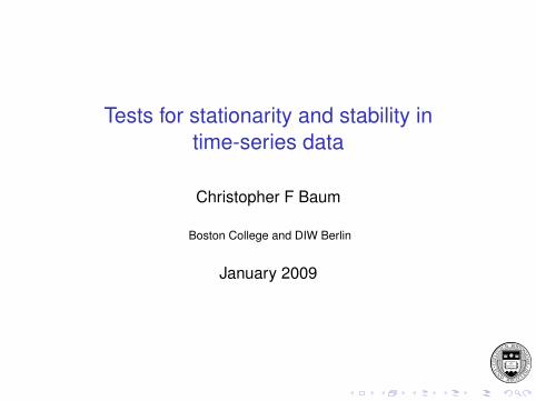
The dfgls command is now part of official Stata. Its originalimplementation was provided by Baum (STB-57, 2000) andBaum and Sperling (STB-58, 2000). dfgls performs theElliott–Rothenberg–Stock (ERS) efficient test for anautoregressive unit root. This test is similar to an (augmented)Dickey-Fuller t test, as performed by dfuller, but has the bestoverall performance in terms of small-sample size and power,dominating the ordinary Dickey-Fuller test. The dfgls test“has substantially improved power when an unknown mean ortrend is present” (ERS, p. 813).

The dfgls varname command applies a generalized leastsquares (GLS) detrending (demeaning) step to the varname:

ydt = yt − β

′zt

For detrending, zt = (1, t)′

and β0, β1 are calculated byregressing [y1, (1− αL) y2, ..., (1− αL) yT ] onto[z1, (1− αL) z2, ..., (1− αL) zT ] where α = 1 + c/T withc = −13.5, and L is the lag operator. For demeaning, zt = (1)′

and the same regression is run with c = −7.0.

The values of c are chosen so that “the test achieves the powerenvelope against stationary alternatives (is asymptotically MPI(most powerful invariant)) at 50 percent power” (Stock,Handbook of Econometrics, 1994, p. 2769).

The dfgls varname command applies a generalized leastsquares (GLS) detrending (demeaning) step to the varname:

ydt = yt − β

′zt

For detrending, zt = (1, t)′

and β0, β1 are calculated byregressing [y1, (1− αL) y2, ..., (1− αL) yT ] onto[z1, (1− αL) z2, ..., (1− αL) zT ] where α = 1 + c/T withc = −13.5, and L is the lag operator. For demeaning, zt = (1)′

and the same regression is run with c = −7.0.

The values of c are chosen so that “the test achieves the powerenvelope against stationary alternatives (is asymptotically MPI(most powerful invariant)) at 50 percent power” (Stock,Handbook of Econometrics, 1994, p. 2769).

The augmented Dickey-Fuller regression is then computedusing the yd

t series:

∆ydt = α + γt + ρyd

t−1 +m∑

i=1

δi∆ydt−i + εt

where m =maxlag. The notrend option suppresses the timetrend in this regression.

Approximate critical values for the GLS detrended test aretaken from ERS, Table 1 (p. 825). Approximate critical valuesfor the GLS demeaned test are identical to those applicable tothe no-constant, no-trend Dickey-Fuller test, and are computedusing the dfuller code.

The augmented Dickey-Fuller regression is then computedusing the yd

t series:

∆ydt = α + γt + ρyd

t−1 +m∑

i=1

δi∆ydt−i + εt

where m =maxlag. The notrend option suppresses the timetrend in this regression.

Approximate critical values for the GLS detrended test aretaken from ERS, Table 1 (p. 825). Approximate critical valuesfor the GLS demeaned test are identical to those applicable tothe no-constant, no-trend Dickey-Fuller test, and are computedusing the dfuller code.

The maxlag(p) option specifies the maximum lag order to beconsidered. The test statistics will be calculated for each lag upto the maximum lag order (which may be zero). If not specified,the maximum lag order for the test is by default calculated fromthe sample size using a rule provided by Schwert (JBES, 1989)using c=12 and d=4 in his terminology. Whether the maximumlag is explicitly specified or computed by default, the samplesize is held constant over lags at the maximum availablesample.

The dfgls routine includes a very powerful lag selectioncriterion, the “modified AIC” (MAIC) criterion proposed by Ngand Perron (Econometrica, 2000). They have established thatuse of this MAIC criterion may provide “huge sizeimprovements” (2000, abstract) in the dfgls test. Thecriterion, indicating the appropriate lag order, is printed ondfgls’ output, and may be used to select the test statistic fromwhich inference is to be drawn.

The maxlag(p) option specifies the maximum lag order to beconsidered. The test statistics will be calculated for each lag upto the maximum lag order (which may be zero). If not specified,the maximum lag order for the test is by default calculated fromthe sample size using a rule provided by Schwert (JBES, 1989)using c=12 and d=4 in his terminology. Whether the maximumlag is explicitly specified or computed by default, the samplesize is held constant over lags at the maximum availablesample.

The dfgls routine includes a very powerful lag selectioncriterion, the “modified AIC” (MAIC) criterion proposed by Ngand Perron (Econometrica, 2000). They have established thatuse of this MAIC criterion may provide “huge sizeimprovements” (2000, abstract) in the dfgls test. Thecriterion, indicating the appropriate lag order, is printed ondfgls’ output, and may be used to select the test statistic fromwhich inference is to be drawn.

It should be noted that all of the lag length criteria employed bydfgls (the sequential t test of Ng and Perron, the SchwarzCriterion (SC), and the MAIC) are calculated, for various lags,by holding the sample size fixed at that defined for the longestlag. These criteria cannot be meaningfully compared over laglengths if the underlying sample is altered to use all availableobservations. That said, if the optimal lag length (by whatevercriterion) is found to be much less than that picked by theSchwert criterion, it would be advisable to rerun the test withthe maxlag option specifying that optimal lag length, especiallywhen using samples of modest size.

The KPSS test

As an alternative to the Dickey–Fuller style tests for stationarity,we may consider the KPSS test of Kwiatkowski, Phillips,Schmidt and Shin (J. Econometrics, 1992). This test (and thosederived from it) have the more “natural” null hypothesis ofstationarity (I(0)), where a rejection indicates non-stationarity(I(1) or I(d)). The KPSS test may be used to confirm thefindings of a DF-GLS test; their verdicts will not necessarilyagree, but if they do, that is strong evidence in favor of(non-)stationarity.

The kpss command (findit kpss to install) performs theKPSS test for stationarity of a time series. The test may beconducted under the null of either trend stationarity (the default)or level stationarity. Inference from this test is complementary tothat derived from those based on the Dickey–Fuller distribution(such as dfgls, dfuller and pperron). The KPSS test isoften used in conjunction with those tests to investigate thepossibility that a series is fractionally integrated (that is, neitherI(1) nor I(0)): see Lee and Schmidt (J. Econometrics, 1996).

The series is detrended (demeaned) by regressing y onzt = (1, t)

′ (zt = (1)′

), yielding residuals et . Let the partial sum

series of et be st . Then the zero-order KPSS statistic is

k0 =T−2 ∑T

t=1 s2t

T−1∑T

t=1 e2t

For maxlag> 0, the denominator is computed as theNewey-West estimate of the long run variance of the series;see [R] newey. Approximate critical values for the KPSS testare taken from KPSS (1992).

The kpss routine has been enhanced to add two optionsrecommended by the work of Hobijn et al. (EconometricInstitute WP, Rotterdam, 1998). An automatic bandwidthselection routine has been added, rendering it unnecessary toevaluate a range of test statistics for various lags. An option toweight the empirical autocovariance function by the QuadraticSpectral kernel, rather than the Bartlett kernel employed byKPSS, has also been introduced.

These options may be used separately or in conjunction. It is inconjunction that Hobijn et al. found the greatest improvement inthe test: “Our Monte Carlo simulations show that the best smallsample results of the test in case the process exhibits a highdegree of persistence are obtained using both the automaticbandwidth selection procedure and the Quadratic Spectralkernel.” (1998, p.14)

The kpss routine has been enhanced to add two optionsrecommended by the work of Hobijn et al. (EconometricInstitute WP, Rotterdam, 1998). An automatic bandwidthselection routine has been added, rendering it unnecessary toevaluate a range of test statistics for various lags. An option toweight the empirical autocovariance function by the QuadraticSpectral kernel, rather than the Bartlett kernel employed byKPSS, has also been introduced.

These options may be used separately or in conjunction. It is inconjunction that Hobijn et al. found the greatest improvement inthe test: “Our Monte Carlo simulations show that the best smallsample results of the test in case the process exhibits a highdegree of persistence are obtained using both the automaticbandwidth selection procedure and the Quadratic Spectralkernel.” (1998, p.14)

Covariate-augmented unit root tests

Returning to the DF-GLS unit root test, we now consider animproved version of that test proposed by Elliott and Jansson(J. Econometrics, 2003) that adds stationary covariates to gainadditional power.

As is well known in the applied economics literature, even a testwith DF-GLS’s favorable characteristics may still lack power todistinguish between the null hypothesis of nonstationarybehavior (I(1)) and the stationary alternative (I(0)). In manyapplications, using a longer time series is not feasible due toknown structural breaks, institutional changes, and the like.

Another potential alternative, the panel unit root test, brings itsown set of complications (do we assume all series are I(1)? orthat all are I(0)?).









Elliott and Jansson addressed this issue by considering amodel in which there is one potentially nonstationary (I(1))series, y , which potentially covaries with some availablestationary variables, x . This idea was first put forth by BruceHansen in 1995 who proposed a covariate augmented D–Ftest, or CADF test and showed that this test had greater powerthan those which ignored the covariates.

The authors extended Hansen’s results to show that such a testcould be conducted in the presence of unknown nuisanceparameters, and with constants and trends in the model. Theirproposed test may be readily calculated by estimating a vectorautoregression (var) in the {y , x} variables and performing asequence of matrix manipulations.

Elliott and Jansson addressed this issue by considering amodel in which there is one potentially nonstationary (I(1))series, y , which potentially covaries with some availablestationary variables, x . This idea was first put forth by BruceHansen in 1995 who proposed a covariate augmented D–Ftest, or CADF test and showed that this test had greater powerthan those which ignored the covariates.

The authors extended Hansen’s results to show that such a testcould be conducted in the presence of unknown nuisanceparameters, and with constants and trends in the model. Theirproposed test may be readily calculated by estimating a vectorautoregression (var) in the {y , x} variables and performing asequence of matrix manipulations.

The model considered is:

zt = β0 + β1t + ut , t = 1, . . . , T

A(L)

((1− ρL)uy ,t

ux ,t

)= et

with zt = {yt , x ′t}′, xt an m × 1 vector,

β0 = {βy0, β′x0}′, β1 = {βy1, β

′x1}′ and ut = {uy ,t , u′

x ,t}′.

A(L) is a stable matrix polynomial of finite order k in the lagoperator L.

This is a vector autoregression (VAR) in the model of x and thequasi-difference of y . The relevant test is that the parameter ρis equal to unity, implying that y has a unit root, againstalternatives that ρ is less than one.

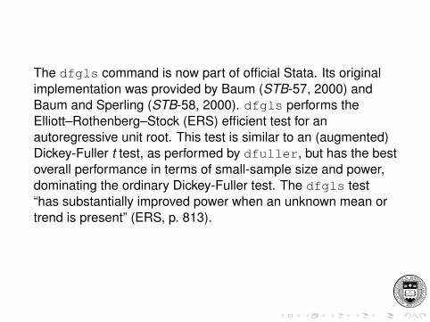
The model considered is:

zt = β0 + β1t + ut , t = 1, . . . , T

A(L)

((1− ρL)uy ,t

ux ,t

)= et

with zt = {yt , x ′t}′, xt an m × 1 vector,

β0 = {βy0, β′x0}′, β1 = {βy1, β

′x1}′ and ut = {uy ,t , u′

x ,t}′.

A(L) is a stable matrix polynomial of finite order k in the lagoperator L.

This is a vector autoregression (VAR) in the model of x and thequasi-difference of y . The relevant test is that the parameter ρis equal to unity, implying that y has a unit root, againstalternatives that ρ is less than one.

The potential gain in this test depends on the R2 between yand the set of x covariates. As Elliott and Pesavento (J. Money,Credit, Banking 2006) point out, the relevant issue is the abilityof a unit root test to have power to distinguish between I(1) anda local alternative. The local alternative is in terms ofc = T (ρ− 1) where ρ is the largest root in the ARrepresentation of y .

How far below unity must ρ fall to give a unit root test the abilityto discern stationary, mean-reverting behavior (albeit withstrong persistence, with ρ > 0.9) from nonstationary, unit rootbehavior? The various tests in this literature differ in their poweragainst relevant local alternatives.

The potential gain in this test depends on the R2 between yand the set of x covariates. As Elliott and Pesavento (J. Money,Credit, Banking 2006) point out, the relevant issue is the abilityof a unit root test to have power to distinguish between I(1) anda local alternative. The local alternative is in terms ofc = T (ρ− 1) where ρ is the largest root in the ARrepresentation of y .

How far below unity must ρ fall to give a unit root test the abilityto discern stationary, mean-reverting behavior (albeit withstrong persistence, with ρ > 0.9) from nonstationary, unit rootbehavior? The various tests in this literature differ in their poweragainst relevant local alternatives.

The c parameter can be expressed in terms of the half-life (k )of a shock, where a unit root implies an infinite half-life:k = log(0.5)/ log(ρ). When related to the local alternative,k/T = log(0.5)/c. For about 120 observations (30 years ofquarterly data), c = −5 corresponds to a half-life of 16.8 timeperiods (over four years at a quarterly frequency). From Elliott,Rothenberg, Stock (ERS, Econometrica, 1996), the standardDickey-Fuller test (dfuller)has 12% power to reject thealternative. The ERS DF-GLS test (dfgls) has 32% power.

In contrast, with an R2 = 0.2, the Elliott–Jansson (EJ) test haspower of 42%. The power rises to 53% (69%) for R2 = 0.4(0.6). For higher absolute values of c (shorter half-lives), thegains are smaller. For c = −10, or a half-life of 8.4 periods, thepower of the D-F (DF-GLS) test is 31% (75%). The EJ test haspower of 88%, 94% and 99% for R2 = 0.2, 0.4, 0.6. One clearconclusion: DF-GLS always has superior power compared todfuller.

The c parameter can be expressed in terms of the half-life (k )of a shock, where a unit root implies an infinite half-life:k = log(0.5)/ log(ρ). When related to the local alternative,k/T = log(0.5)/c. For about 120 observations (30 years ofquarterly data), c = −5 corresponds to a half-life of 16.8 timeperiods (over four years at a quarterly frequency). From Elliott,Rothenberg, Stock (ERS, Econometrica, 1996), the standardDickey-Fuller test (dfuller)has 12% power to reject thealternative. The ERS DF-GLS test (dfgls) has 32% power.

In contrast, with an R2 = 0.2, the Elliott–Jansson (EJ) test haspower of 42%. The power rises to 53% (69%) for R2 = 0.4(0.6). For higher absolute values of c (shorter half-lives), thegains are smaller. For c = −10, or a half-life of 8.4 periods, thepower of the D-F (DF-GLS) test is 31% (75%). The EJ test haspower of 88%, 94% and 99% for R2 = 0.2, 0.4, 0.6. One clearconclusion: DF-GLS always has superior power compared todfuller.

Like other unit root tests, you must specify the deterministicmodel assumed for y . As in dfgls, you can specify that themodel contains no deterministic terms, a constant, or constantand trend. But as the Elliott–Jansson model contains one ormore x variables as well, you may also specify that thosevariables’ deterministic model contains no deterministic terms,a constant, or constant and trend.

Five cases are defined:1. No constant nor trend in model

2. Constant in y only3. Constants in both {y , x}4. Constant and trend in y , constant in x5. No restrictions


Five cases are defined:1. No constant nor trend in model2. Constant in y only

3. Constants in both {y , x}4. Constant and trend in y , constant in x5. No restrictions


Five cases are defined:1. No constant nor trend in model2. Constant in y only3. Constants in both {y , x}

4. Constant and trend in y , constant in x5. No restrictions


Five cases are defined:1. No constant nor trend in model2. Constant in y only3. Constants in both {y , x}4. Constant and trend in y , constant in x

5. No restrictions


Five cases are defined:1. No constant nor trend in model2. Constant in y only3. Constants in both {y , x}4. Constant and trend in y , constant in x5. No restrictions

The urcovar Stata command implements the EJ test usingMata to perform a complicated sequence of matrixmanipulations that produce the test statistic. EJ’s Table 1 ofasymptotic critical values is stored in the program and used toproduce a critical value corresponding to the R2 for your data.The command syntax:

urcovar depvar varlist [if exp] [in range] [ , maxlag(#) case[#)firstobs ]

where the case option specifies the deterministic model, withdefault of case 1. The maxlag option specifies the number oflags to be used in computing the VAR (default 1). Thefirstobs option specifies that the first observation of depvarshould be used to define the first quasi-difference (rather thanzero). The urcovar command is available for Stata 9.2 orStata 10 via findit urcovar.

As an illustration of urcovar use, we consider an experimentsimilar to that tested in EJ, who in turn refer to aBlanchard–Quah model. The variable of interest is U.S.personal income (PINCOME). The single stationary covariate tobe considered is the U.S. unemployment rate (UNRATE). Bothare acquired from the FRED database with the fredusecommand (Drukker, Stata Journal, 2006) and have beenconverted to the common quarterly frequency for1950Q2–1987Q4 using tscollap (Baum, STB-57, 2000).

We first present a line plot of these two series, then the outputfrom a conventional DF-GLS test, followed by the output fromurcovar, cases 3 and 5. The maxlag considered in both thedfgls and urcovar tests is set to eight quarters.

2

2

24

4

46

6

68

8

810

10

10Unemployment Rate

Unem

ploy

men

t Ra

te

Unemployment Rate0

0

01000

1000

10002000

2000

20003000

3000

30004000

4000

4000Personal Income

Pers

onal

Inco

me

Personal Income1950q1

1950q1

1950q11960q1

1960q1

1960q11970q1

1970q1

1970q11980q1

1980q1

1980q11990q1

1990q1

1990q1Quarter

Quarter

QuarterPersonal Income

Personal Income

Personal IncomeUnemployment Rate

Unemployment Rate

Unemployment Rate

. dfgls PINCOME, maxlag(8) trend

DF-GLS for PINCOME Number of obs = 142

DF-GLS tau 1% Critical 5% Critical 10% Critical[lags] Test Statistic Value Value Value

8 -0.830 -3.519 -2.875 -2.5937 -0.585 -3.519 -2.890 -2.6076 -0.173 -3.519 -2.905 -2.6205 -0.071 -3.519 -2.918 -2.6334 -0.272 -3.519 -2.932 -2.6453 -0.334 -3.519 -2.944 -2.6562 0.332 -3.519 -2.955 -2.6661 0.655 -3.519 -2.966 -2.676

Opt Lag (Ng-Perron seq t) = 8 with RMSE 11.44531Min SC = 5.103851 at lag 3 with RMSE 11.96667Min MAIC = 5.000489 at lag 7 with RMSE 11.56349

. urcovar PINCOME UNRATE, maxlag(8) case(3)

Elliott-Jansson unit root test for PINCOME 1950q2 - 1987q4Number of obs: 143Stationary covariates: UNRATEDeterministic model: Case 3Maximum lag order: 8

Estimated R-squared: 0.9950H0: rho = 1 [ PINCOME is I(1) ]H1: rho < 1 [ PINCOME is I(0) ]Reject H0 if Lambda < critical value

Lambda: 11.83075% critical value: 17.9900

. urcovar PINCOME UNRATE, maxlag(8) case(5)

Elliott-Jansson unit root test for PINCOME 1950q2 - 1987q4Number of obs: 143Stationary covariates: UNRATEDeterministic model: Case 5Maximum lag order: 8

Estimated R-squared: 0.8407H0: rho = 1 [ PINCOME is I(1) ]H1: rho < 1 [ PINCOME is I(0) ]Reject H0 if Lambda < critical value

Lambda: 17.15585% critical value: 29.1170

The DF-GLS test is unable to reject its null of I(1) at anyreasonable level of significance. When we augment the testwith the stationary covariate in the EJ test, quite differentresults are forthcoming. Case 3 allows for constant terms (butno trends) in both the quasi-difference of PINCOME andUNRATE. The R2 in this system is over 0.99. Case 5 allowsconstant terms and trends in both equations of the VAR, withan R2 of 0.84.

Like the DF-GLS test, the EJ test has a null hypothesis ofnonstationarity (I(1)). The EJ test statistic, λ, must becompared with the interpolated 5% critical value. A value of λsmaller than the tabulated value leads to a rejection, and viceversa. In both cases, we may reject the null hypothesis at the95% level of confidence in favor of the alternative hypothesis ofstationarity.

The DF-GLS test is unable to reject its null of I(1) at anyreasonable level of significance. When we augment the testwith the stationary covariate in the EJ test, quite differentresults are forthcoming. Case 3 allows for constant terms (butno trends) in both the quasi-difference of PINCOME andUNRATE. The R2 in this system is over 0.99. Case 5 allowsconstant terms and trends in both equations of the VAR, withan R2 of 0.84.

Like the DF-GLS test, the EJ test has a null hypothesis ofnonstationarity (I(1)). The EJ test statistic, λ, must becompared with the interpolated 5% critical value. A value of λsmaller than the tabulated value leads to a rejection, and viceversa. In both cases, we may reject the null hypothesis at the95% level of confidence in favor of the alternative hypothesis ofstationarity.

Unit root tests allowing for structural breaks

Unit root tests are particularly susceptible to breaks in thestructure of a relationship. For instance, the hypothesis ofpurchasing power parity (PPP) in international trade impliesthat real exchange rates should be stationary stochasticprocesses. A vast literature contains numerous instanceslacking support for this hypothesis (e.g., Baum et al., J. Intl.Money and Fin., 2001).

One rationale that has been put forth for rejection of the PPPhypothesis is the existence of structural breaks. In this section,we discuss how standard unit root tests may be modified toallow for structural breaks.

Unit root tests allowing for structural breaks

Unit root tests are particularly susceptible to breaks in thestructure of a relationship. For instance, the hypothesis ofpurchasing power parity (PPP) in international trade impliesthat real exchange rates should be stationary stochasticprocesses. A vast literature contains numerous instanceslacking support for this hypothesis (e.g., Baum et al., J. Intl.Money and Fin., 2001).

One rationale that has been put forth for rejection of the PPPhypothesis is the existence of structural breaks. In this section,we discuss how standard unit root tests may be modified toallow for structural breaks.

Perron and Vogelsang (JBES, 1992), building on work byPerron (JBES, 1990), demonstrate that nonrejection of theunit-root hypothesis may be “associated with an apparentpermanent change in the level of the series” (1992, p. 302). AsPerron demonstrated with a simulation experiment, “...if themagnitude of the change is significant, one could hardly rejectthe unit-root hypothesis even if the series would consist of i .i .d .disturbances around a deterministic component (albeit one witha shift in mean)...The problem is one of modelmisspecification.” (1990, p.155)

To deal with this source of bias in unit-root tests, Perron andVogelsang propose a class of test statistics which allow for twoalternative forms of change: the additive outlier (AO) model,capturing a sudden change, and the innovational outlier (IO)model, appropriate for modeling a gradual shift in the mean ofthe series.

Perron and Vogelsang (JBES, 1992), building on work byPerron (JBES, 1990), demonstrate that nonrejection of theunit-root hypothesis may be “associated with an apparentpermanent change in the level of the series” (1992, p. 302). AsPerron demonstrated with a simulation experiment, “...if themagnitude of the change is significant, one could hardly rejectthe unit-root hypothesis even if the series would consist of i .i .d .disturbances around a deterministic component (albeit one witha shift in mean)...The problem is one of modelmisspecification.” (1990, p.155)

To deal with this source of bias in unit-root tests, Perron andVogelsang propose a class of test statistics which allow for twoalternative forms of change: the additive outlier (AO) model,capturing a sudden change, and the innovational outlier (IO)model, appropriate for modeling a gradual shift in the mean ofthe series.

The test statistics do not require a priori knowledge of thebreakpoint, as their computation involves search over thesample for a single break date. The breakpoint, should it occur,is denoted by Tb, 1 < Tb < T , where T is the sample size. TheAO model considers the dynamics of yt to be given by

yt = δDTbt + yt−1 + wt , t = 2, ..., T (1)

with DTbt = 1 for t = Tb + 1, and 0 otherwise, under the nullhypothesis of a unit root. Under the alternative hypothesis,

yt = c + δDUt + vt , t = 2, ..., T (2)

where DUt = 1 for t > Tb, and 0 otherwise.

This more general specification nests the null hypothesis (1) inthe case that the distribution of vt may be factored into a unitroot and a stationary ARMA process. The test strategy is thento estimate the regression

yt = µ + δDUt + yt (3)

the residuals of which (yt) are regressed on their lagged values,lagged differences, and a set of dummy variables, the latterneeded to ensure that the distribution of the test statistic will bemanageable:

yt =k∑

i=0

ωiDTbt−i +αyt−1 +k∑

i=1

θi∆yt−i +et , t = k +2, ..., T (4)

This regression, similar in nature to the common AugmentedDickey–Fuller (ADF) model, yields an estimate of α which willbe significantly less than one in the presence of stationarity.Perron and Vogelsang provide critical values and describe themethod by which they may be simulated.

The equivalent process for the innovational outlier (IO) modelexpresses the shock (for instance, the effect of δ in (1) above)as having the same effect on yt as any other shock, so that thedynamic effects of DTb have the same ARMA representation asdo other shocks to the model.

This regression, similar in nature to the common AugmentedDickey–Fuller (ADF) model, yields an estimate of α which willbe significantly less than one in the presence of stationarity.Perron and Vogelsang provide critical values and describe themethod by which they may be simulated.

The equivalent process for the innovational outlier (IO) modelexpresses the shock (for instance, the effect of δ in (1) above)as having the same effect on yt as any other shock, so that thedynamic effects of DTb have the same ARMA representation asdo other shocks to the model.

This formulation, when transformed, generates the finite ARmodel

yt = µ+δDUt +ϑDTbt +αyt−1 +k∑

i=1

θi∆yt−i +et , t = k +2, ..., T

(5)which again yields a test of α differing from one in the presenceof stationarity. In both the AO and the IO models, theappropriate values of Tb (the breakpoint) and k (theautoregressive order) are unknown. This is resolved for Tb byestimating the model for each feasible breakpoint, and followingone of several proposed rules to identify the optimal singlebreakpoint. In our application, we search for the minimumt-statistic on δ. Conditional on that Tb, the autoregressive orderk is chosen, as Perron (1990) suggests, by a sequence of pairsof F-tests for the significance of lags, starting from anappropriately large maximum order.

The unit-root test statistics forthcoming from the AO and IOmodels will account for one-time level shifts which mightotherwise be identified as departures from stationarity.However, the behavior of real exchange rate series over oursample period may not be adequately characterized by a singleshift; as Lothian (JIMF, 1998) has noted, US dollar-based realexchange rates appear to have exhibited two shifts in meanover the 1980-1987 period, approximately reverting to theirpre-1980 level after 1987. In these circumstances, allowing fora single level shift will not suffice.

The Perron–Vogelsang methodology has been extended todouble mean shifts by Clemente et al. (Econ.Letters, 1988),who demonstrate that a two-dimensional grid search forbreakpoints (Tb1 and Tb2) may be used for either the AO or IOmodels, and provide critical values for the tests. In this context,the AO model involves the estimation of:

yt = µ + δ1DU1t + δ2DU2t + yt (6)

and subsequently searching for the minimal t−ratio for thehypothesis α = 1 in the model:

yt =k∑

i=0

ωiDTb1,t−i

k∑i=0

ωiDTb2,t−i + αyt−1 +k∑

i=1

θi∆yt−i + et , (7)

t = k + 2, ..., T

For the IO model, the modified equation to be estimatedbecomes:

yt = µ + δ1DU1t + δ2DU2t + ϑ1DTb1,t + ϑ2DTb2,t + (8)

αyt−1 +k∑

i=1

θi∆yt−i + et , t = k + 2, ..., T

with a search for the minimal t−ratio for the hypothesis α = 1.These tests customarily are applied to a trimmed sample; wetrimmed 5% of the sample from each end when searching forthe breakpoints.

In Baum et al. (JIFMIM, 1999), the results from thesetwo-mean-break models are quite consistent over 17 countriesand both CPI and WPI price series. In none of the 58 casesconsidered do the unit-root test statistics surpass theirapproximate 5% critical values, although the t-statistics for δ1and δ2 generally indicate the presence of meaningful level shiftsin almost every instance.

Even with structural breaks taken into account, the evidence infavor of nonstationarity is overwhelmingly strong and consistentacross countries for both CPI-based and WPI-based realexchange rate series.

In Baum et al. (JIFMIM, 1999), the results from thesetwo-mean-break models are quite consistent over 17 countriesand both CPI and WPI price series. In none of the 58 casesconsidered do the unit-root test statistics surpass theirapproximate 5% critical values, although the t-statistics for δ1and δ2 generally indicate the presence of meaningful level shiftsin almost every instance.

Even with structural breaks taken into account, the evidence infavor of nonstationarity is overwhelmingly strong and consistentacross countries for both CPI-based and WPI-based realexchange rate series.

Therefore, we may conclude that the inability to reject theunit-root hypothesis for the post-Bretton Woods era usingstandard univariate unit-root tests is not likely to be overturnedby allowing for one or two mean breaks in the series. Suchinstability is quite apparent in a first-order Markov model of thereal exchange rate, but even when unit-root tests are adjustedfor its presence, the null hypothesis of nonstationarity cannotbe rejected in favor of mean reversion.

These routines for unit root tests in the presence of structuralbreaks are available as Stata commands clemao1,clemao2, clemio1, clemio2. To install, finditclemao.

Therefore, we may conclude that the inability to reject theunit-root hypothesis for the post-Bretton Woods era usingstandard univariate unit-root tests is not likely to be overturnedby allowing for one or two mean breaks in the series. Suchinstability is quite apparent in a first-order Markov model of thereal exchange rate, but even when unit-root tests are adjustedfor its presence, the null hypothesis of nonstationarity cannotbe rejected in favor of mean reversion.

These routines for unit root tests in the presence of structuralbreaks are available as Stata commands clemao1,clemao2, clemio1, clemio2. To install, finditclemao.

A general test for structural stability: qll

Elliott and Müller’s 2006 paper in Review of Economic Studies(EM) addresses the large literature on testing a time seriesmodel for structural stability. They consider “tests of the nullhypothesis of a stable linear model

yt = X ′t β + Z ′

t γ + ε

against the alternative of a partially unstable model

yt = X ′t βt + Z ′

t γ + ε

where the variation in βt is of the strong form” (p. 907), ornontrivial.

Consideration of this alternative has led to a huge literaturebased on the “diversity of possible ways {βt} can benon-constant.” EM point out that optimal tests and theirasymptotic distributions have not been derived for manyparticular models of the alternative.

Their approach develops a single unified framework, noting thatthe “seemingly different approaches of ‘structural breaks’ and‘random coefficients’ are in fact equivalent.” (p.908) EM unifythe approaches that describe a breaking process with anumber of non-random parameters with tests that specifystochastic processes for {βt} without requiring to specify itsexact evolution.

Consideration of this alternative has led to a huge literaturebased on the “diversity of possible ways {βt} can benon-constant.” EM point out that optimal tests and theirasymptotic distributions have not been derived for manyparticular models of the alternative.

Their approach develops a single unified framework, noting thatthe “seemingly different approaches of ‘structural breaks’ and‘random coefficients’ are in fact equivalent.” (p.908) EM unifythe approaches that describe a breaking process with anumber of non-random parameters with tests that specifystochastic processes for {βt} without requiring to specify itsexact evolution.

The processes considered include breaks that occur in arandom fashion, serial correlation in the changes of thecoefficients, a clustering of break dates, and so on. Under anormality assumption on the disturbances, “small sampleefficient tests in this broad set are asymptotically equivalent”and “leaving the exact breaking process unspecified (apartfrom a scaling parameter) does not result in a loss of power inlarge samples.” (p. 908)

The consequences of this approach to the problem of structuralstability are profound. “The equivalence of power over manymodels means that there is little point in deriving further optimaltests for particular processes in our set” (p. 908) and theresearcher can carry out (almost) efficient inference withoutspecifying the exact path of the breaking process.

Furthermore, the computation of EM’s Quasi-Local Level (qLL)test statistic is straightforward, and it remains valid for verygeneral specifications of the error term and covariates. Thecomputation requires no more than (k + 1) OLS regressions fora model with k covariates, in contrast to many approacheswhich require T or T 2 regressions. No arbitrary trimming of thedata is required.

The consequences of this approach to the problem of structuralstability are profound. “The equivalence of power over manymodels means that there is little point in deriving further optimaltests for particular processes in our set” (p. 908) and theresearcher can carry out (almost) efficient inference withoutspecifying the exact path of the breaking process.

Furthermore, the computation of EM’s Quasi-Local Level (qLL)test statistic is straightforward, and it remains valid for verygeneral specifications of the error term and covariates. Thecomputation requires no more than (k + 1) OLS regressions fora model with k covariates, in contrast to many approacheswhich require T or T 2 regressions. No arbitrary trimming of thedata is required.

In the structural break literature, a fixed number of N breaks atτ1, . . . , τN are assumed. Much of the literature addressesN = 1: e.g. the “Chow test”, cusums tests ofBrown–Durbin–Evans, Bai and Perron, Andrews and Ploberger,etc.

In contrast, the time-varying parameter literature considers arandom process generating βt : often considered as a randomwalk process. The approaches of Leybourne and McCabe,Nyblom, and Saikkonen and Luukonen are based on classicalstatistics, while Koop and Potter and Giordani et al. consider aBayesian approach. All of these approaches are veryanalytically challenging.

EM argue that tests for one of these phenomena will havepower against the other, and vice versa. Therefore a singleapproach will suffice.







EM raise the interesting question: why do we test for parameterconstancy? They consider three motivations:

1. Stability relates to theoretical constructs such as the Lucascritique of economic policymaking

2. Forecasting will depend crucially on a stable relationship3. Standard inference on β will be useless if {βt} varies in a

permanent fashion; persistent changes will render a fixedmodel misleading

“The more pervasive these three motivations are, the morepersistent the changes in {β}.” (p. 912) Therefore, EM proposethat a useful test should maximize its power against persistentchanges in {βt}.



2. Forecasting will depend crucially on a stable relationship

3. Standard inference on β will be useless if {βt} varies in apermanent fashion; persistent changes will render a fixedmodel misleading

















The conditions underlying the EM test allow for diversebreaking models, from relatively rare (including a single break)to very frequent small breaks (such as breaks every period withprobability p). Breaks can also occur with a regular pattern,such as every 16 quarters following U.S. presidential elections.

Computation of the qLL test statistic is straightforward, relyingonly on OLS regressions and construction of an estimate of thelong-run covariance matrix of {Xtεt}. For uncorrelated εt , arobust covariance matrix will suffice. For possiblyautocorrelated εt , a HAC (Newey–West) covariance matrix isappropriate.

The null hypothesis of parameter stability is rejected for smallvalues of qLL: that is, values more negative than the criticalvalues. Asymptotic critical values are provided by EM fork = 1, . . . , 10 and are independent of the dimension of Zt (theset of covariates assumed to have stable coefficients).







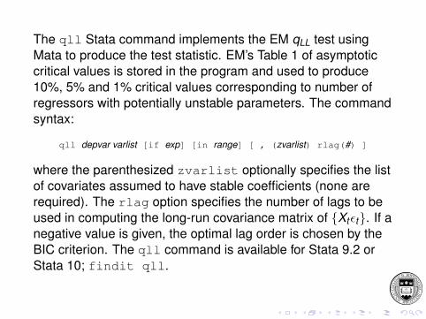
The qll Stata command implements the EM qLL test usingMata to produce the test statistic. EM’s Table 1 of asymptoticcritical values is stored in the program and used to produce10%, 5% and 1% critical values corresponding to number ofregressors with potentially unstable parameters. The commandsyntax:

qll depvar varlist [if exp] [in range] [ , (zvarlist) rlag(#) ]

where the parenthesized zvarlist optionally specifies the listof covariates assumed to have stable coefficients (none arerequired). The rlag option specifies the number of lags to beused in computing the long-run covariance matrix of {Xtεt}. If anegative value is given, the optimal lag order is chosen by theBIC criterion. The qll command is available for Stata 9.2 orStata 10; findit qll.

We consider a regression of inflation on the laggedunemployment rate, the Treasury bill rate and the Treasurybond rate. We assume the latter two coefficients are stableover the period. We test over the full sample and a 1990–2000subsample.

4

4

46

6

68

8

810

10

1012

12

12Unemployment Rate

Unem

ploy

men

t Ra

te

Unemployment Rate0

0

05

5

510

10

1015

15

15CPI Inflation

CPI I

nfla

tion

CPI Inflation1960q1

1960q1

1960q11970q1

1970q1

1970q11980q1

1980q1

1980q11990q1

1990q1

1990q12000q1

2000q1

2000q1date

date

dateCPI Inflation

CPI Inflation

CPI InflationUnemployment Rate

Unemployment Rate

Unemployment Rate

. qll inf L.UR (TBILL TBON), rlag(8)

Elliott--Müller qLL test statistic for time varying coefficientsin the model of inf, 1960q1 - 2000q4Allowing for time variation in 1 regressorsH0: all regression coefficients fixed over the sample period (N = 164)

Test stat. 1% Crit.Val. 5% Crit.Val. 10% Crit.Val.-2.260 -11.05 -8.36 -7.14

Long-run variance computed with 8 lags.

. qll inf L.UR (TBILL TBON) if tin(1990q1,), rlag(8)

Elliott-Müller qLL test statistic for time varying coefficientsin the model of inf, 1990q1 - 2000q4Allowing for time variation in 1 regressorsH0: all regression coefficients fixed over the sample period (N = 44)

Test stat. 1% Crit.Val. 5% Crit.Val. 10% Crit.Val.-6.647 -11.05 -8.36 -7.14

Long-run variance computed with 8 lags.

In both samples, using eight lags to calculate the long-runcovariance matrix, the null hypothesis that the coefficients onthe lagged unemployment rate (L.UR) are stable cannot berejected at the 10% level of confidence. The Elliott–Müller qLLtest indicates that the stability of this regression model, allowingfor instability in the coefficient of the unemployment rate only,cannot be rejected by the data.

Tests for stationarity and stability in time-series datafm · Tests for stationarity and stability in time-series data Christopher F Baum Boston College and DIW Berlin ... The dfgls

Documents