Notes on Stationarity and extremum principles in mechanics (with applications to optimal design) Pauli Pedersen Department of Mechanical Engineering, Solid Mechanics Technical University of Denmark Nils Koppels All` e, Building 404, DK-2800 Kgs.Lyngby, Denmark email: [email protected] WORKING PRINT December 9, 2008

Welcome message from author
This document is posted to help you gain knowledge. Please leave a comment to let me know what you think about it! Share it to your friends and learn new things together.
Transcript
Notes on
Stationarity and extremum
principles in mechanics(with applications to optimal design)
Pauli PedersenDepartment of Mechanical Engineering, Solid Mechanics
Technical University of DenmarkNils Koppels Alle, Building 404, DK-2800 Kgs.Lyngby, Denmark
email: [email protected] PRINT
December 9, 2008

ii c©Pauli Pedersen: Stationarity and extremum principles in mechanics
Stationarity and extremumprinciples in mechanics
Copyright c©2008 by Pauli Pedersen,
ISBN 06
PrefaceThe energy principles in mechanics play an important role, not only for anal-ysis but also for design synthesis and optimization. However, when teachingmechanics it is mostly found difficult to communicate a basic understandingof these principles.
What is the reason for this situation that so many teachers agree with?Should the reason be related to the students, to the teachers, or to the avail-able textbooks? The present small book attempts to give an alternative non-traditionally presentation of the subject. The presentation in chapters 2 - 6 hasearlier been used in a course on elasticity, anisotropy and laminates.
A primary idea is to separate the mathematical derivation of an iden-tity from the specific interpretations of this identity. Then also separate thestationarity principles from the extremum principles, and finally balance thephysical interpretation of the non-physical variations, where also the aspect ofinfinitesimal variations is important. Hopefully, this alternative presentationwill appeal to some readers.
The chapters 7 - 9 with direct relation to optimal design use to a largeextend the basic principles in mechanics, but also introduces new results fromdesign variations, i.e., the sensitivity analysis for design. These chapters areinfluences by recently published papers, and here serve as examples to il-lustrate the simplicities that may results from using the basic principles inmechanics.
Kgs. Lyngby, Winter 2008
Pauli Pedersen
iii

iv c©Pauli Pedersen: Stationarity and extremum principles in mechanics
Contents
Preface iii
Contents v
1 Introduction 11.1 Background . . . . . . . . . . . . . . . . . . . . . . . . . . . . . . 11.2 Layout of contents . . . . . . . . . . . . . . . . . . . . . . . . . . 1
2 Stationarity principlesin mechanics 32.1 The work equation, an identity . . . . . . . . . . . . . . . . . . . . 32.2 Symbols and definitions . . . . . . . . . . . . . . . . . . . . . . . . 42.3 Real stress field and real displacement field . . . . . . . . . . . . . 62.4 Real stress field and virtual displacement field . . . . . . . . . . . . 72.5 Virtual stress field and real displacement field . . . . . . . . . . . . 82.6 Summing up . . . . . . . . . . . . . . . . . . . . . . . . . . . . . . 9
3 Extremum principlesin mechanics 113.1 Principle of minimum total potential energy . . . . . . . . . . . . . 113.2 Principle of minimum total
complementary(stress) potential energy . . . . . . . . . . . . . . . 143.3 Overview of principles and their relations . . . . . . . . . . . . . . 143.4 Summing up . . . . . . . . . . . . . . . . . . . . . . . . . . . . . . 16
4 Potential relations and derivatives 174.1 Equilibrium . . . . . . . . . . . . . . . . . . . . . . . . . . . . . . 174.2 Relations with power law elasticity . . . . . . . . . . . . . . . . . . 184.3 Derivatives of elastic potentials . . . . . . . . . . . . . . . . . . . . 184.4 Summing up . . . . . . . . . . . . . . . . . . . . . . . . . . . . . . 19
5 Energy densitiesin matrix notation 215.1 Strain and stress energy densities . . . . . . . . . . . . . . . . . . . 215.2 Energy densities in
1D non-linear elasticity . . . . . . . . . . . . . . . . . . . . . . . . 225.3 Energy densities in
2D and 3D non-linear elasticity . . . . . . . . . . . . . . . . . . . . 245.4 Summing up . . . . . . . . . . . . . . . . . . . . . . . . . . . . . . 26
v
vi c©Pauli Pedersen: Stationarity and extremum principles in mechanics
6 Elastic energy in beam models 276.1 Elastic energy in a straight beam . . . . . . . . . . . . . . . . . . . 276.2 Results for simple (Bernoulli-Euler) beams . . . . . . . . . . . . . 296.3 Beam solutions by stress(complementary)
principles . . . . . . . . . . . . . . . . . . . . . . . . . . . . . . . 306.4 Summing up . . . . . . . . . . . . . . . . . . . . . . . . . . . . . . 31
7 Some necessary conditions for optimality 337.1 Non-constrained problems . . . . . . . . . . . . . . . . . . . . . . 337.2 Problems with a single constraint . . . . . . . . . . . . . . . . . . . 347.3 Size optimization for stiffness and strength . . . . . . . . . . . . . . 34
7.3.1 Size design with optimal stiffness . . . . . . . . . . . . . . 347.3.2 Size design with optimal strength . . . . . . . . . . . . . . 35
7.4 Shape optimization for stiffness and strength . . . . . . . . . . . . . 357.4.1 Shape design with optimal stiffness . . . . . . . . . . . . . 367.4.2 Shape design with optimal strength . . . . . . . . . . . . . 37
7.5 Conditions with asimple shape parametrization . . . . . . . . . . . . . . . . . . . . . 387.5.1 Possible iterative procedure . . . . . . . . . . . . . . . . . 40
7.6 Summing up . . . . . . . . . . . . . . . . . . . . . . . . . . . . . . 41
8 Analytical beam design 438.1 Optimality criterion for beam design . . . . . . . . . . . . . . . . . 44
8.1.1 Treated boundary conditions and loads . . . . . . . . . . . 468.1.2 Solutions in general . . . . . . . . . . . . . . . . . . . . . 47
8.2 Bernoulli-Euler cantilever beams . . . . . . . . . . . . . . . . . . . 488.2.1 Optimal compliances . . . . . . . . . . . . . . . . . . . . . 49
8.3 Timoshenko cantilever beams . . . . . . . . . . . . . . . . . . . . . 498.3.1 Design of beams with n = 1 cross sections . . . . . . . . . . 50
8.4 Examples of beam cross sections . . . . . . . . . . . . . . . . . . . 548.5 Summing up . . . . . . . . . . . . . . . . . . . . . . . . . . . . . . 54
9 The ultimate optimal material 579.1 The individual constitutive parameters . . . . . . . . . . . . . . . . 579.2 Sensitivity analysis . . . . . . . . . . . . . . . . . . . . . . . . . . 579.3 Final optimization . . . . . . . . . . . . . . . . . . . . . . . . . . . 589.4 Numerical aspects and comparison
with isotropic material . . . . . . . . . . . . . . . . . . . . . . . . 599.5 Summing up . . . . . . . . . . . . . . . . . . . . . . . . . . . . . . 59
References 61
Index 63
Chapter 1
Introduction1.1 BackgroundThe authors background for the present notes are years of teaching energy princi-ples in a course on elasticity, based on (Pedersen 1998a). As stated in the prefaceit is mostly found difficult to communicate a basic understanding of these princi-ples. However, when succeeding, the students has an important tool for many futureapplications.
With a research background in optimal design, the unification that can be ob-tained using energy principles is found important, especially when the design sen-sitivity analysis is build on these principles. The obtained results are then valid for1D, 2D and 3D problems, for anisotropy as well as for isotropy, often for non-linearas well as non linear elasticity, and for analytically research as well as for numericalresearch, see (Pedersen 1998b).
With the present notes, the notions in earlier notes and papers are unified. Lim-iting these notes to mostly analytically derivations without numerically results, thetotal number of pages are few, but hopefully not too dry.
1.2 Layout of contentsIn (Pedersen 1998a) the present chapters 2 and 3 are combined in a single chapter,but it is found advantageously to separate the stationarity principles in chapter 2 withfocus on the principle of virtual work. This principle is of most importance andis based on only a few assumptions, but with a rather abstract interpretation andtherefore not immediately easy to communicate.
Chapter 3 contains a graphical overview of the stationarity as well as the ex-tremum principles. The extremum principles are mainly used as arguments for choos-ing approximations based on a stationarity principle.
The main assumption behind chapter 4 is a proportionality relation between com-plementary energy (stress energy) and strain energy. From this follows proportion-ality relations between total potentials, strain energy, stress energy, external poten-tial, and compliance. The names of stress energy and complementary energy areused synonymously, but in the notations only the superscript σ is applied, not thesuperscript C as in (Pedersen 1998a). Focus is thus put on the fact that comple-mentary principles have stress/force as the primary variables, while strain principleshas strain/displacement as the primary variable and superscript ε is applied for theirrelated quantities.
General simple first order design sensitivities is a result of derivatives on the
1
2 c©Pauli Pedersen: Stationarity and extremum principles in mechanics
energy level. These results are obtained in fields of fixed strains or fixed stresses,and these results do not involve approximations. Chapter 4 is earlier published as anappendix in (Pedersen 2003).
To be specific about the proportionality relation between strain energy and stressenergy, chapter 5 presents a power law elasticity model, that is the most simple exten-sion from linear elasticity. For this reversible model secant stiffnesses as well as tan-gent stiffnesses are derived for a three dimensional model, covering also anisotropicmaterials.
Although being a one dimensional model, the beam is among the most importantstructural elements. It is therefore natural to include as an example in chapter 6, theuse of energy principles in a linear elastic straight beam. These handbook formulasare applied in chapter 8 for design optimization.
Before this design optimization a number of necessary conditions for design op-timization are needed. The description in chapter 7 also focuses on the use of super-elliptic description of shapes in two dimensional models, a description which hasoften been successfully applied.
Chapter 8 contains results from recent research, see (Pedersen and Pedersen2008), and demonstrates that optimal design based directly on an energy approachhas promising aspects. It has been possible to find analytically described optimalbeam designs, even for short beams where the Timoshenko beam theory must beused.
The notes finish with chapter 9 on ultimate optimal material, related to compli-ance optimization,. i.e., again for an energy objective. The results in the referenceresearch (Bendsøe, Guedes, Haber, Pedersen and Taylor 1994) are extended to bevalid for non linear elastic materials as in (Pedersen 1998a). In active research on op-timal design, this free material model is expected to play a major role. In the presentnotes this is taken as a further example on the importance of energy approaches,added design sensitivity analysis.
Chapter 2
Stationarity principlesin mechanics
Energy principles play a central role in mechanics, but surprisingly few books treat Goal ofthe chapterthe subject in a structured way. It is difficult to get an overview of the many different
principles, and important questions are not presented, especially in relation to thenecessary conditions for a certain principle.
The present chapter is written as an alternative to the classical presentations, as by(Langhaar 1962) and (Washizu 1975). We shall show that all principles are specificinterpretations of the same identity, and necessary conditions will not be introduceduntil absolutely needed. We shall refer only to a Cartesian 3-D coordinate system, Tensor
notationand traditional tensor notation for summation and differentiation is applied.
2.1 The work equation, an identityWithout physical interpretation of the quantities involved, we shall derive an impor- No physical
interpretationtant identity. The superscripts a and b are only part of the names (not powers) andtheir use will be explained later. From
σaijε
bij = σa
ij
(
εbij −
1
2(vb
i,j + vbj,i)
)
+ σaij
1
2(vb
i,j + vbj,i) (2.1)
and
σaijv
bj,i = σa
jivbi,j = (σa
ji − σaij)v
bi,j + σa
ijvbi,j (2.2)
follows∫
Vσa
ijεbijdV −
∫
Vσa
ij
(
εbij −
1
2(vb
i,j + vbj,i)
)
dV −∫
V
1
2(σa
ji − σaij)v
bi,jdV −
∫
Vσa
ijvbi,jdV = 0 (2.3)
In (2.3) V is the volume of the domain of interest. Now let A be the surface that Using thetheorem ofdivergence
bounds this domain and nj the outward normal at a point of the surface. Then, usingthe theorem of divergence, the last part of (2.3) is rewritten to∫
Vσa
ijvbi,jdV =
∫
V
(
(σaijv
bi ),j − σa
ij,jvbi
)
dV =
∫
Aσa
ijvbi njdA −
∫
Vσa
ij,jvbi dV
(2.4)
3
4 c©Pauli Pedersen: Stationarity and extremum principles in mechanics
Once more, by adding and subtracting the same quantities, we obtain the iden-tity from which the stationarity principles of mechanics can be read without furthercalculationsThe
identity ∫
Vσa
ijεbijdV −
∫
Vσa
ij
(
εbij −
1
2(vb
i,j + vbj,i)
)
dV −∫
V
1
2(σa
ji − σaij)v
bi,jdV −
∫
A(σa
ij − T ai )vb
i dA −∫
AT a
i vbi dA+
∫
V(σa
ij,j + pai )v
bi dV −
∫
Vpa
i vbi dV = 0 (2.5)
With the superscripts a and b we have indicated certain relations, and we shallnow assume that all quantities with index a are related and that all quantities withindex b are related. However, no relations exist between quantities with differentindex, and the equations therefore still have no physical interpretations.
Let εbij = εb
ij(x) be a strain field derived from a displacement field vbi = vb
i (x)with small strain assumption (engineering strains, linear strains, Cauchy strains)
εbij =
1
2(vb
i,j + vbj,i) (small strain assumption) (2.6)
and let σaij = σa
ij(x) be a stress field with moment and force equilibrium with thefield of volume forces pa
i = pai (x) and surface traction’s T a
i = T ai (x)
σaij = σa
ji
σaij,j = −pa
i
σaijnj = T a
i (2.7)
With (2.6) and (2.7) the identity (2.5) reduces toThe workequation ∫
Vσa
ijεbijdV =
∫
AT a
i vbi dA +
∫
Vpa
i vbi dV (2.8)
which is often called the work equation, although it is merely an identity and doesnot express physical work when the a and b fields are not related.
2.2 Symbols and definitionsFor a better overview, the stationarity principles of mechanics are divided into fourReal
fields groups covering the possible combinations of real fields (indexed by a superscript 0)and virtual fields (without index).
The virtual fields are assumed to be sufficiently differentiable and admissible,Virtualfields but otherwise arbitrary and non-physical. An admissible displacement field must be
kinematically admissible, i.e. it must satisfy the boundary conditions. An admissiblestress field must be statically admissible, i.e., it must satisfy force equilibrium.
A somewhat repeated definition of the quantities in the energy principles may beuseful before the individual principles are stated and proved, all by specific interpre-tations of the work equation (2.8).Geometry variables:
V = Volume of the continuum or structureA = Surface area that bounds the volume V (2.9)
Stationarity principles 5
State variables at position x in the volume:
εij = εij(x) = description of strain state at position x
σij = σij(x) = description of stress state at position x
Ti = Ti(x) = surface traction = force (per unit area) in direction i at position x of A
pi = pi(x) = force (per unit volume) in direction i at position x in V(2.10)
Work and energy quantities in strains and displacements:Work ofexternal loads
W ε = W ε(vi) =
∫
A
∫ vi
0Ti(vi)dvidA +
∫
V
∫ vi
0pi(vi)dvidV
Strainenergy density
uε = uε(εij) =
∫ εij
0σij(εij)dεij
Totalstrain energy
U ε =
∫
VuεdV
Total potentialenergy
Πε = U ε − W ε (2.11)
Complementary work and energy quantities in stresses and forces: Complementarywork ofexternal loadsW σ = W σ(Ti, pi) =
∫
A
∫ Ti
0vi(Ti)dTidA +
∫
V
∫ pi
0vi(pi)dpidV
Stressenergy density
uσ = uσ(σij) =
∫ σij
0εij(σij)dσij
Totalstress energy
Uσ =
∫
VuσdV
Total potentialcomplementaryenergyΠσ = Uσ − W σ (2.12)
Compliance relations: Compliance ofexternal loads
Φ = W ε(dead loads, i.e.,W σ = 0) =
∫
ATividA +
∫
VpividV
Compliancefromelastic energyΦ = U ε + Uσ = W ε + W σ
Compliancefrompotential ofexternal loads
Φ = −Uext (2.13)
6 c©Pauli Pedersen: Stationarity and extremum principles in mechanics
2.3 Real stress field and real displacement fieldAs a first example of use of the work equation (2.8) we insert the real stress field σ0
ij
in equilibrium with the real load field T 0i , p0
i , and the real displacement field v0i from
which the real strain field ε0ij is derived. We get
∫
Vσ0
ijε0ijdV =
∫
AT 0
i v0i dA +
∫
Vp0
i v0i dV (2.14)
For arbitrary constitutive relations we have
σ0ijε
0ij =
∫ σ0ijε0ij
0d(σij εij) =
∫ ε0ij
0σij(εij)dεij +
∫ σ0ij
0εij(σij)dσij (2.15)
which, together with the definitions in (2.11) - (2.12), gives
σ0ijε
0ij = uε0 + uσ0
∫
Vσ0
ijε0ijdV = U ε0 + Uσ0 (2.16)
Analogously for the external loads we get∫
AT 0
i v0i dA +
∫
Vp0
i v0i dV = W ε0 + W σ0 (2.17)
and (2.14) can thus be writtenZero sumof totalpotentials U ε0 + Uσ0 − (W ε0 + W σ0) = Πε0 + Πσ0 = 0 (2.18)
i.e., the sum of the real total potentials is zero.Especially for a linear elastic material the definitions in (2.11) - (2.12) give
U ε0 = Uσ0 =1
2
∫
Vσ0
ijε0ijdV (2.19)
In relation to the nature of the external forces, the concept of dead load is impor-tant. For dead loads the forces are independent of the displacement of their point ofaction, say a gravity load. For a dead load we get no complementary(stress) work,W σ0 = 0, and the work is thus
W ε0 =
∫
AT 0
i v0i dA +
∫
Vp0
i v0i dV
assuming W σ0 = 0 (dead load) (2.20)
For a system with both linear elasticity and dead loads (2.14) givesClapeyron’stheorem
U ε0 =1
2W ε0 (2.21)
and thus
Πε0 := U ε0 − W ε0 = −1
2W ε0 = −U ε0 (2.22)
which is often called Clapeyron’s theorem for linear elasticity. The ”missing” energyW ε0/2 is assumed to be dissipated before the static equilibrium with which we areconcerned.
Note, that if we by definition take −W ε0 as given by (2.20) to be the externalExternalpotentialandcompliance
potential Uext, then the assumption of dead load is not necessary, but then againexternal potential is hardly a physical quantity. The quantity W ε0 as given by (2.20)is also named the compliance, i.e., Φ as defined in (2.13).
Stationarity principles 7
2.4 Real stress field and virtual displacement fieldAssume that vi is a kinematically admissible displacement field and that εij is thestrain field derived from vi. Furthermore, as before, σ0, T 0
i , p0i are the real stress,
surface traction and volume force fields. Then the work equation (2.8) reads∫
Vσ0
ijεijdV =
∫
AT 0
i vidA +
∫
Vp0
i vidV (2.23)
To distinguish the work by the external loads from the work of the reactions wedivide the surface area A into
A = AT + Av (2.24)
where AT is the surface area without displacement control and Av is the surface areawith given kinematic conditions. Furthermore, we describe the virtual field vi by avariation δvi relative to the real field v0
i
vi = v0i + δvi, εij = ε0
ij + δεij (2.25)
which with εij = (vi,j + vj,i)/2 gives
δεij =1
2(δvi,j + δvj,i) (2.26)
Now, as vi is assumed to be kinematically admissible, we have δvi = 0 on thesurface Av (but not necessarily vi = 0) , and thus (2.23) with (2.14) reduces to Virtual
workprinciple
∫
Vσ0
ijδεijdV =
∫
AT
T 0i δvidA +
∫
Vp0
i δvidV (2.27)
This is called the virtual work principle or the principle of virtual displacements.Note that the virtual displacements and strains in (2.27) are infinitesimal and expressenergy and work variations without assumptions of linearity. Note also that the virtualwork principle is a principle about a state, not a process.
Often (2.23) and even (2.8) are also called the virtual work principle, but in thisbook we shall assume the virtual displacements and the virtual strains to beinfinitesimal.
Because stresses are fixed in the virtual work principle, a direct physical inter-pretation is not clear. However, it can be read as an energy balance which is valid forany kinematically admissible disturbance of the displacement field.
Some specific cases of use of the virtual work principle lead us to specializedprinciples. Let us choose the very specific virtual displacement field
δvi = ∆v corresponding to the single load Q
δvi = 0 corresponding to all other external loads∆εij derived from this field (2.28)
Castigliano’s1st theoremthen (2.27) reduces to
∫
Vσ0
ij∆εijdV = Q∆v or Q =∆U ε
∆v=
∂U ε
∂v(2.29)
which is the first theorem of Castigliano. It is useful in determining stiffnesses. Note,that this theorem is valid independent of the specific constitutive behaviour (σ =
8 c©Pauli Pedersen: Stationarity and extremum principles in mechanics
σ(ε)). The force Q should be interpreted as a generalized force; thus, if Q is anexternal moment, then v is the corresponding rotation.
Now a much used theorem is obtained from (2.29) if we assume linear elasticity,because then we can set the displacement to ∆v = 1 and ∆εij = ε1
ij for the resultingstrains from this unit displacement field and get
Q =
∫
Vσ0
ijε1ijdV (2.30)
Unitdisplacementtheorem forlinearelasticity
Returning to general non-linear elastic materials, we can interpret the virtualwork principle as stationary potential energy. A potential is a scalar from whichwork can be derived. Let us assume that a material has a potential and the externalloads has as well, then (2.29) statesStationary
totalpotentialenergy
δU ε = δW ε or δΠε = 0 (2.31)
2.5 Virtual stress field and real displacement fieldA virtual stress field σij is a statically admissible field, i.e., in equilibrium with thegiven external loads. Now, inserting also the real displacement field v0
i , and derivedstrain field ε0
ij in (2.27), we get∫
Vσijε
0ijdV =
∫
AT
T 0i v0
i dA +
∫
Av
Tiv0i dA +
∫
Vp0
i v0i dV (2.32)
On the surface Av, the surface traction’s Ti are the unknown reactions. Takingthe virtual stress field as
σij = σ0ij + δσij (2.33)
where σ0ij is the real stress field and δσij is an infinitesimal virtual stress field satis-
fying
δσij = δσji, δσij,j = 0
δσijnj = δTi where δTi = 0 on AT (2.34)
then using (2.14) we getStressvirtual workprinciple
∫
Vδσijε
0ijdV =
∫
Av
Tiv0i dA (2.35)
which expresses the principle of complementary(stress) virtual work, also called theprinciple of virtual stresses.
Choosing a specific virtual field
δσij = ∆σij where ∆σijnj = ∆Q corresponding to displacement v
∆T = ∆σijnj = 0 for all other places with prescribed vi 6= 0 (2.36)
Stationarity principles 9
we get from (2.35)
∫
V∆σijε
0ijdV = ∆Qv or v =
∆Uσ
∆Q=
∂Uσ
∂Q(2.37)
Castigliano’s2nd theoremwhich is the second theorem named after Castigliano. It is valuable in determining
flexibilities.Unit loadtheorem forlinearelasticity
Also, a unit theorem is obtained in complementary(stress) energies, read directlyfrom (2.37) when linear elasticity is assumed, i.e., ∆Q = 1 and ∆σij = σ1
ij
v =
∫
Vσ1
ijε0ijdV (2.38)
Stationarytotal stresspotentialenergy
Finally, the parallel to stationary potential energy is the principle of stationarycomplementary(stress) potential energy
δUσ = δW σ or δΠσ = 0 (2.39)
2.6 Summing up• The identity (2.5) is obtained by rather simple mathematics and has no physical
interpretation.
• The work equation (2.8) involve two independent fields. A stress/force fieldin equilibrium, these fields are given super index a. A displacement field withderived strain field, these fields are given super index b.
• Work as well as complementary work must in general be determined by inte-gration and therefore depend on the force/displacement function.
• Strain energy density as well as stress energy density is also determined byintegration, applying the constitutive relation.
• The notion of compliance is important in optimal design formulations and istherefore specifically defined.
• With real stress field and virtual displacement field we get the virtual workprinciple, and from this a number of more specific principles. The virtualwork principle is a principle about a state, not a process.
• With virtual stress field and real displacement field we get the complementaryvirtual work principle (stress virtual work principle), and from this a numberof more specific complementary principles.
• Virtual displacements and virtual stresses are in general infinitesimal.

10 c©Pauli Pedersen: Stationarity and extremum principles in mechanics
Chapter 3
Extremum principlesin mechanics
The stationarity principles of mechanics are based on very few assumptions. Theprinciples of virtual work hold for any constitutive model and for any type of load,and for potential systems these virtual principles give stationary potential energies. Motivation
forextremum
Many approximation methods (like the finite element method) are based on anduniquely specified by these stationarity principles. However, this does not give ussufficient reason to choose an approximate solution that satisfies the same stationar-ity as the unknown real solution. Energy principles that in addition to stationaritygive extremum can justify our choice. We choose the approximation for which theenergy is closest to the real unknown energy. Furthermore, consistent approximationmethods are a reasonable choice also for problems where an extremum cannot beproved.
3.1 Principle of minimum total potential energyWe shall firstly prove the principle of minimum total potential energy δ2Π > 0, and Assumptionsfor this we need assumptions concerning the constitutive model as well as for the loadbehaviour. Let us start with a single load Q (force or moment) and the correspond-ing displacement v (translation or rotation). For this force Q as a function of thecorresponding displacement v, we will assume the following single load behaviour Single force
behaviour∂Q
∂v≥ 0,
∂v
∂Q> 0, Q(v = 0) = 0 (3.1)
as illustrated in Figure 3.1a).We note that Q(v) is a function but, as ∂Q/∂v = 0 is a possibility, v(Q) is not
strictly a function. Non-linearity and change of sign for curvature is possible. Fromthe definition of W ε and W σ in (2.11) - (2.12) follows
W ε =
∫ v
0Q(v)dv ⇒ ∂W ε
∂v= Q = Q(v)
W σ =
∫ Q
0v(Q)dQ ⇒ ∂W σ
∂Q= v = v(Q) (3.2)
As by (2.17) we have for this case of a single force
W ε + W σ = Qv (3.3)
11
12 c©Pauli Pedersen: Stationarity and extremum principles in mechanics
PSfrag replacements
vv
Q
v
Q
W ε
W σ
W ε
va vb
(W ε)a
(W ε)b
a
b
W ε
v= Qa
W ε
v= Qb
a) b)
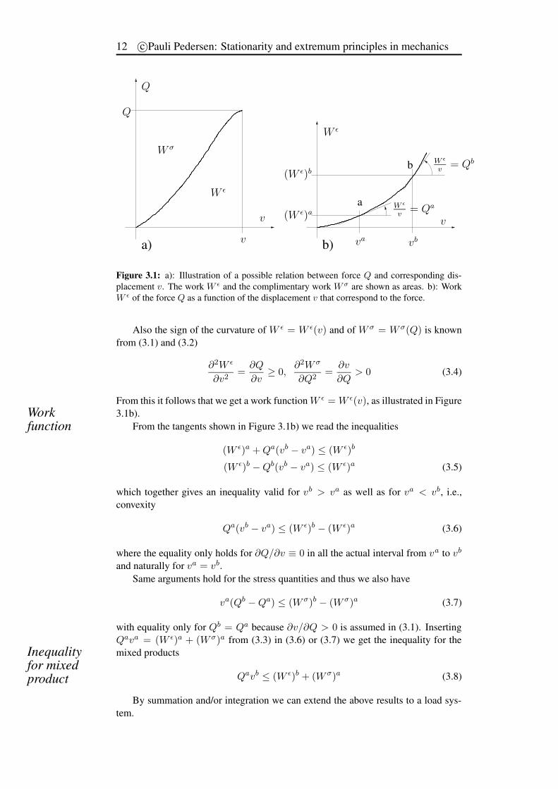
Figure 3.1: a): Illustration of a possible relation between force Q and corresponding dis-placement v. The work W ε and the complimentary work W σ are shown as areas. b): WorkW ε of the force Q as a function of the displacement v that correspond to the force.
Also the sign of the curvature of W ε = W ε(v) and of W σ = W σ(Q) is knownfrom (3.1) and (3.2)
∂2W ε
∂v2=
∂Q
∂v≥ 0,
∂2W σ
∂Q2=
∂v
∂Q> 0 (3.4)
From this it follows that we get a work function W ε = W ε(v), as illustrated in Figure3.1b).Work
function From the tangents shown in Figure 3.1b) we read the inequalities
(W ε)a + Qa(vb − va) ≤ (W ε)b
(W ε)b − Qb(vb − va) ≤ (W ε)a (3.5)
which together gives an inequality valid for vb > va as well as for va < vb, i.e.,convexity
Qa(vb − va) ≤ (W ε)b − (W ε)a (3.6)
where the equality only holds for ∂Q/∂v ≡ 0 in all the actual interval from va to vb
and naturally for va = vb.Same arguments hold for the stress quantities and thus we also have
va(Qb − Qa) ≤ (W σ)b − (W σ)a (3.7)
with equality only for Qb = Qa because ∂v/∂Q > 0 is assumed in (3.1). InsertingQava = (W ε)a + (W σ)a from (3.3) in (3.6) or (3.7) we get the inequality for themixed productsInequality
for mixedproduct Qavb ≤ (W ε)b + (W σ)a (3.8)
By summation and/or integration we can extend the above results to a load sys-tem.
Extremum principles 13
For a uniaxial stress/strain in terms of pure normal (σ, ε) or, alternatively, pureshear (τ, γ), we assume a function very parallel to the load displacement function(3.1),
∂σ
∂ε> 0,
∂ε
∂σ> 0, σ(ε = 0) = 0 (3.9)
Uniaxialconstitutivemodel
i.e., well-defined functions for σ = σ(ε) as well as for ε = ε(σ) because strictinequalities hold in (3.9). From the assumptions (3.9) follows in direct analogy to theload-work arguments which lead to (3.6)-(3.8)
σa(εb − εa) < uεb − uεa for εb 6= εa
εa(σb − σa) < uσb − uσa for σb 6= σa
σaεb < uεb + uσa for a 6= b (3.10)
with the definitions of energy densities in (2.11) - (2.12) and the previously discussedrelation uε + uσ = σε as stated in (2.16).
For a multidimensional stress/strain state a direct generalization is not easy, andthe assumption is therefore often stated directly as convexity of the energy density inthe six-dimensional strain/stress spaces. With tensor symbols this is written
σaij(ε
bij − εa
ij) < uεb − uεa for εbij 6= εa
ij
εaij(σ
bij − σa
ij) < uσb − uσa for σbij 6= σa
ij
σaijε
bij < uεb + uσa for a 6= b and
σijεij = uε + uσ for a = b (3.11)
Generalstress/strainstate
We now have the necessary inequalities to prove the extremum principles, andagain we start from the work equation (2.8). With real stresses σ0
ij and virtual dis-placements, strains (vi − v0
i ), (εij − ε0ij) we get
∫
Vσ0
ij(εij − ε0ij)dV =
∫
AT 0
i (vi − v0i )dA +
∫
Vp0
i (vi − v0i )dV (3.12)
From (3.11) follows that the left-hand side satisfies∫
Vσ0
ij(εij − ε0ij)dV < U ε − U ε0 for εij 6= ε0
ij (3.13)
and the right-hand side for dead loads (∂T 0i /∂vi = 0, ∂p0
i /∂vi = 0) gives∫
AT 0
i (vi − v0i )dA +
∫
Vp0
i (vi − v0i )dV = W ε − W ε0 (3.14)
Using (3.13) as well as (3.14) in (3.12) we get the result Minimumpotential
U ε − U ε0 > W ε − W ε0 or Πε > Πε0 for εij 6= ε0ij (3.15)
i.e., the extremum principle for total potential energy. We note that the dead loadassumption (3.14) is a necessary condition if we do not decide by definition to termthe right-hand side of (3.12) as the negative external potential energy.
14 c©Pauli Pedersen: Stationarity and extremum principles in mechanics
3.2 Principle of minimum totalcomplementary(stress) potential energy
We can directly establish the complementary(stress) principle because all the neces-sary inequalities were derived in the Section 3.1. In the work equation (2.8) we nowinsert v0
i , ε0ij and the virtual stresses σij and get
∫
Vε0ij(σij − σ0
ij)dV =
∫
Av0i (Ti − T 0
i )dA +
∫
Vv0i (pi − p0
i )dV (3.16)
The left-hand side satisfies∫
Vε0ij(σij − σ0
ij)dV < Uσ − Uσ0 for σij 6= σ0ij (3.17)
The main part of the right-hand side is zero when σij is statically admissiblebecause pi −p0
i = 0 and Ti −T 0i can only be different from zero at the reactions. For
dead loads this part will be W σ − W σ0, and with (3.17) in (3.16) we getMinimumcomplementary(stress)potential
Uσ − Uσ0 > W σ − W σ0 or Πσ > Πσ0 for σij 6= σ0ij (3.18)
i.e., the extremum principle for total complementary(stress) potential energy.Using also the earlier result (2.18) of Πε0 + Πσ0 = 0 for only real fields we can
with (3.15) and (3.18) set up two-sided bounds on approximate solutions. For the realsolution we have (2.18), and by the sum of (3.15) and (3.18) we for an approximatesolution get
Πε + Πσ > 0 or Πε > −Πσ (3.19)
Furthermore, substitution of Πε0 = −Πσ0 in (3.15) and (3.18) then gives thetwo-sided boundsTwo-sided
boundsΠε > Πε0 > −Πσ
Πσ > Πσ0 > −Πε (3.20)
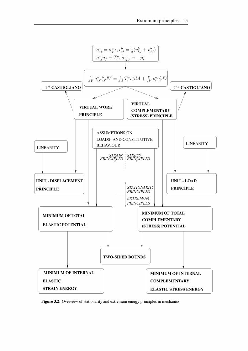
3.3 Overview of principles and their relationsFigure 5.1 illustrate the connections between the many different energy principles.The indicated horizontal dash line shows the division between the stationarity andthe extremum principles. The indicated vertical dash line shows the division betweenthe strain principles and the complementary stress principles.
Extremum principles 15
PSfrag replacements
σaij = σa
jiε, εbij = 1
2(vb
i,j + vbj,i)
σaijnj = T a
i , σaij,j = −pa
i
∫
Vσa
ijεbijdV =
∫
AT a
i vbi dA +
∫
Vpa
i vbi dV
1st CASTIGLIANO 2nd CASTIGLIANO
VIRTUAL WORKPRINCIPLE
VIRTUALCOMPLEMENTARY(STRESS) PRINCIPLE
LINEARITYLINEARITY
ASSUMPTIONS ONLOADS- AND CONSTITUTIVEBEHAVIOUR
UNIT - DISPLACEMENT
PRINCIPLE
UNIT - LOADPRINCIPLE
MINIMUM OF TOTAL
ELASTIC POTENTIAL
MINIMUM OF TOTALCOMPLEMENTARY(STRESS) POTENTIAL
TWO-SIDED BOUNDS
MINIMUM OF INTERNAL
ELASTICSTRAIN ENERGY
MINIMUM OF INTERNALCOMPLEMENTARY
ELASTIC STRESS ENERGY
STRESSPRINCIPLES
STRAINPRINCIPLES
STATIONARITYPRINCIPLESEXTREMUMPRINCIPLES
Figure 3.2: Overview of stationarity and extremum energy principles in mechanics.
16 c©Pauli Pedersen: Stationarity and extremum principles in mechanics
3.4 Summing up• Extremum principles serve as argument for choosing approximate solutions
that satisfy stationarity principles.
• A basic assumption for extremum principles is that a force(moment) is a strictfunction of its corresponding translation(rotation).
• For the constitutive behaviour a basic assumption for extremum principles isconvexity of energy density in the six dimensional strain/stress space.
• The principle of minimum total potential energy and the principle of mini-mum total complementary energy together give two-sided bounds for the realsolution.
• The graphical overview in Figure 5.1 shows stationary as well as extremumprinciples, strain principles as well as stress (complementary) principles.
Chapter 4
Potential relations and derivatives
This chapter shows some important potential relations and then the sensitivity analy-sis directly in energy terms, for linear as well as for non-linear power law elasticity.These results are often used as a basis for other formulations. For detail on the resultsin this chapter see (Pedersen 1998b) and (Masur 1970). Although not new, resultslike (4.10) and (4.14) are not so well known, and not intuitively understandable, Not well known
but importanteven for the case of linear elasticity (p = 1). For optimal design these results giverise to important simplifications.
4.1 EquilibriumThe general equation of energy equilibrium is Energy
equilibriumU ε + Uσ + U ext = 0 (4.1)
with elastic strain energy U ε and elastic stress energy Uσ (elastic complementary en-ergy) from the corresponding densities uε, uσ integrated over the structure/continuumvolume V Internal
potentialsU ε =
∫
VuεdV and Uσ =
∫
VuσdV (4.2)
and the external potential U ext is defined by Externalpotential
U ext := −(∫
ATividA +
∫
VpividV
)
(4.3)
with surface traction’s Ti, volume forces pi , corresponding displacements vi, andarea A surrounding the volume V . The surface traction’s and the volume forcesare assumed to be given. The displacements vi (displacement field) with resultingstrains, stresses and energy densities are the solution for a given design, i.e. thesolution for a given static problem of elasticity. Assumed
power lawelasticity
Power law elastic materials resulting in the density relation uσ = puε everywherein the continuum or structure give in total Uσ = pU ε and the equilibrium (4.1) is thensimplified to
(1 + p)U ε = −U ext (4.4)
with 0 < p ≤ 1 being a material power law constant.
17
18 c©Pauli Pedersen: Stationarity and extremum principles in mechanics
4.2 Relations with power law elasticityDefining the total potential Πε and the total complementary(stress) potential Πσ byTotal
potentialsΠε := U ε + U ext = −Πσ (4.5)
using Πε + Πσ = 0, give from (4.4) the relations
Πε = −pU ε = −Uσ =p
1 + pU ext = −Πσ (4.6)
and by p > 0 and U ε > 0 get Uσ > 0, Πσ > 0, Πε < 0 and U ext < 0. FromPotentialrelations this follows that design for a number of differently stated extremum problems are
equivalent and that their values at the extrema are related as
max Πε = −min Πσ = −min pU ε = −min Uσ = max p
1 + pU ext (4.7)
with p = 1 for the specific case of linear elasticity.
4.3 Derivatives of elastic potentialsThe derivative of the total potential Πε with respect to an arbitrary parameter, say adesign parameter h, is
dΠε/dh = (∂Πε/∂h)fixed strains + (∂Πε/∂ε) (dε/dh) = (∂Πε/∂h)fixed strains (4.8)
because of stationary total potential ∂Πε/∂ε = 0 (virtual work principle) with respectto kinematically admissible strain variations.
For design-independent external loads, (∂U ext/∂h)fixed strains = 0, the definition(4.5) then givesDesign
independentloads (∂Πε/∂h)fixed strains = (∂U ε/∂h)fixed strains (4.9)
and totally from (4.6), (4.8) and (4.9) get the result that is frequently used in designoptimization
dU ε/dh = −1
p(∂U ε/∂h)fixed strains (4.10)
Localdesignparameter
For a local design parameter he that only changes the design in the region e ofthe structure/continuum this gives the possibility of a localized determination of thesensitivity for the total elastic strain energy
dU ε/dhe = −1
p(∂((uε)eVe)/∂he)fixed strains (4.11)
where (uε)e is the mean strain energy density in the region of he and where Ve is thecorresponding volume. Note that the only difference between linear (p = 1) and non-linear material is the factor 1/p, and for a condition on stationarity dU ε/dhe = 0, phas no influence.Remark
Note, that the sensitivity is not physically localized, but still without approxi-mation it is possible to determine the sensitivity localized.
Potential relations 19
For the complementary potentials even more simple results are available
dΠσ/dh = (∂Πσ/∂h)fixed stresses + (∂Πσ/∂σ) (dσ/dh) = (∂Πσ/∂h)fixed stresses(4.12)
because of stationary total complementary potential ∂Πσ/∂σ = 0 (complementaryvirtual work principle) with respect to statically admissible stress variations. FromUσ = Πσ then follows
dUσ/dh = (∂Uσ/∂h)fixed stresses (4.13)
which with the relation p(dU ε/dh) = (dUσ/h) and (4.13), (4.10) gives
(∂Uσ/∂h)fixed stresses = − (∂U ε/∂h)fixed strains (4.14)
valid also for p 6= 1. Formula (4.14) can also be found in the optimal design paperby (Masur 1970).
4.4 Summing up• With proportionality between strain energy and stress energy, simple propor-
tional relations to external potential and to total potentials exist.
• From this follows that sensitivity analyses are simplified, and alternative opti-mization objectives can be chosen.
• First order sensitivities with fixed strain fields or fixed stress fields result fromthe virtual work principle or from the virtual complementary(stress) work prin-ciple.

20 c©Pauli Pedersen: Stationarity and extremum principles in mechanics
Chapter 5
Energy densitiesin matrix notation
For linear strain models {ε}, {δε} are the vectors of strain and variational strain, and{σ}, {δσ} are the vectors of conjugated stress and conjugated variational stress. In Linear strain
notationthis chapter energy densities is described by the linear strain quantities, but a similardescription follows for non-linear strain notation.
5.1 Strain and stress energy densitiesWith {ε}, {δε} being the vectors of strain and variational strain, and {σ}, {δσ} beingthe vectors of conjugated stress and conjugated variational stress; then the variationalstrain energy density δuε is defined by Strain energy
densityδuε = {σ}T {δε} ⇒ uε =
∫ {ε}
0{σ}T {dε} (5.1)
and thus having the same dimension as stress. The tilde ˜ indicate the differencebetween integration variable {ε} and final strain state {ε}, i.e., the stress function is{σ} = {σ({ε})}. The strain energy density is a function of strain, and from the strainenergy density function uε stress is obtained by differentiation
{σ} =duε
{dε} = {σ({ε})} = [L]{ε} (5.2)
and by its definition then the secant modulus [L]. Stress energydensityThe variational stress energy density δuσ is defined by
δuσ = {δσ}T {ε} ⇒ uσ =
∫ {σ}
0{ε}T {dσ} (5.3)
The stress energy density is a function of stress and from the stress energy densityfunction uσ, and the secant compliance relation [L]−1 is obtained by differentiation
{ε} =duσ
{dσ} = {ε({σ})} = [L]−1{σ} (5.4)
Together the definitions of variational strain energy density and variational stressenergy density gives
δ({σ}T {ε}) = δuε + δuσ (5.5)
21
22 c©Pauli Pedersen: Stationarity and extremum principles in mechanics
and with integration from zero elastic energy density to final state follows
uε + uσ = {σ}T {ε} (5.6)
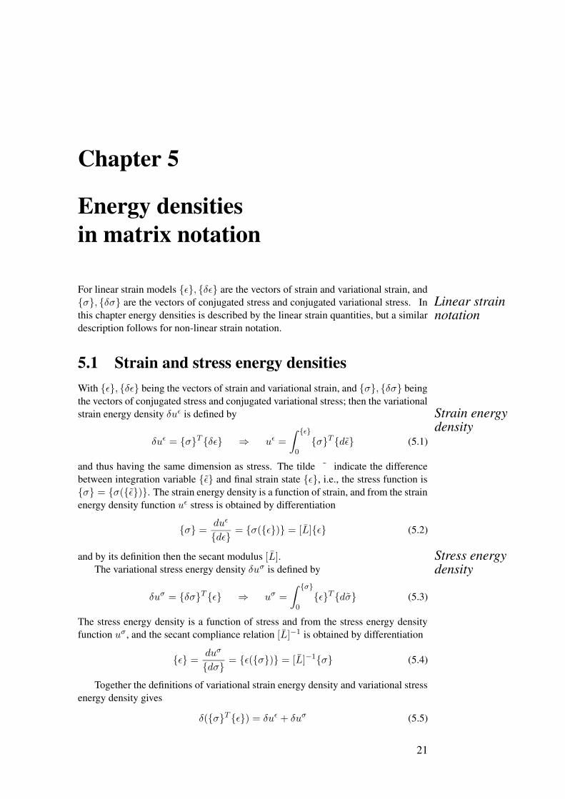
For a one dimensional case Figure 5.1 illustrates the definitions (5.1) and (5.3)by areas, and the relation (5.6) is also directly recognized.
PSfrag replacements
ε
σ
uε
uσ
Figure 5.1: Illustration of strain energy density uε (5.1) and of stress energy density uσ (5.3)by areas.
5.2 Energy densities in1D non-linear elasticity
Power lawelasticity The analysis is restricted to power law non-linear analysis, because for this model
analytical explicit expressions for the constitutive matrices are obtained.Although the general case of 3D anisotropic behaviour is described for this non-
linearity, at first a 1D model is treated. The model of power law non-linear elasticityfor a 1D model in terms of σ = σ(ε) is
σ = Eεp or more general σ = | ε
ε0|p−1E0ε for ε ≥ ε0 (5.7)
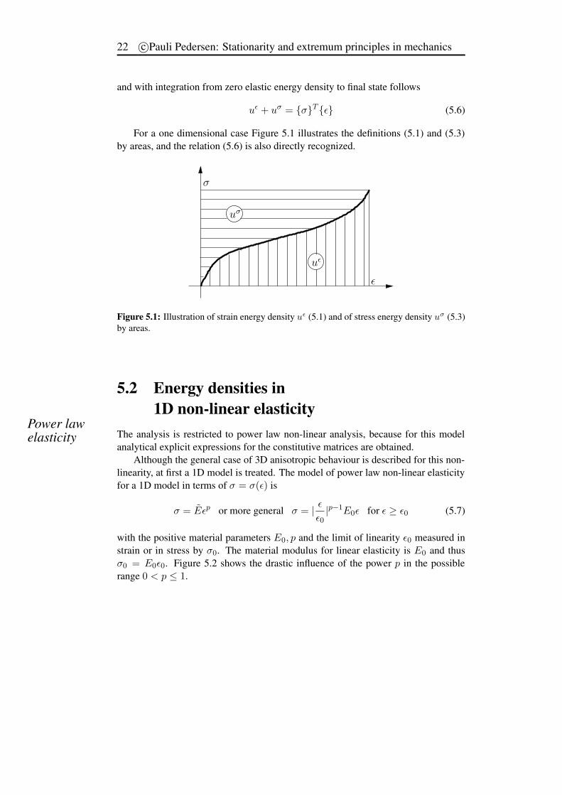
with the positive material parameters E0, p and the limit of linearity ε0 measured instrain or in stress by σ0. The material modulus for linear elasticity is E0 and thusσ0 = E0ε0. Figure 5.2 shows the drastic influence of the power p in the possiblerange 0 < p ≤ 1.
Energy densities in matrix notation 23
0
0.05
0.1
0.15
0.2
0.25
0.3
0.35
0.4
0 0.05 0.1 0.15 0.2 0.25 0.3 0.35 0.4
PSfrag replacements
ε
σE0
= εp
εp−1
0
p = 1.0p = 0.9p = 0.8p = 0.6p = 0.4p = 0.2p = 0.1
ε0
Figure 5.2: Illustration of the influence from power p in the applied power law non linearelasticity. For strains smaller than the limiting strain ε0 a linear behavior is assumed.
Secant andtangentmodulus
For convenience, here ε > 0 is assumed, and it follows that the secant modulusEs and the tangent modulus Et are
Es :=σ
ε= Eεp−1
Et :=dσ
dε= pEεp−1 = pEs (5.8)
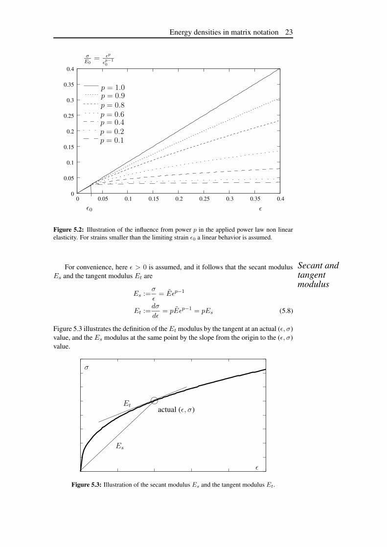
Figure 5.3 illustrates the definition of the Et modulus by the tangent at an actual (ε, σ)value, and the Es modulus at the same point by the slope from the origin to the (ε, σ)value.
PSfrag replacements
ε
σ
Es
Et actual (ε, σ)
Figure 5.3: Illustration of the secant modulus Es and the tangent modulus Et.
24 c©Pauli Pedersen: Stationarity and extremum principles in mechanics
Inserting (5.7) in (5.1), the strain energy density for this material model is ob-tained
uε = E
∫ ε
0εpdε =
1
p + 1Eεp+1 (5.9)
and from (5.6) with (5.21) get
uε + uσ = σε = Eεp+1 ⇒ uσ =p
p + 1Eεp+1 (5.10)
Proportionalrelation The simple proportional relation
uσ = puε (5.11)
between stress energy density and strain energy density often simplifies analysis (andespecially sensitivity analysis for optimal design) to a large extent and give rise toa number of important general results. However, it should be kept in mind that thepower law non-linear elasticity is a restrictive model.
5.3 Energy densities in2D and 3D non-linear elasticity
Effectivestrain/stress Extension to 2D and 3D models is not trivial, and the definitions of effective strain
and of effective stress must be chosen appropriately. In matrix notation the differen-tial strain energy density duε is similar to the variation in (5.1)
duε = {σ}T {dε} (5.12)
In analogy with (5.7) the constitutive secant modulus is
{σ} =
(
εe
ε0
)p−1
E0[α]{ε} ⇒ {σ} = [L]{ε} with [L] =
(
εe
ε0
)p−1
E0[α]
(5.13)
assuming linear elasticity for εe ≤ ε0, and with the non-dimensional and constantmatrix [α] describing the relative moduli (isotropy as well as non-isotropy). TheConstitutive
secantmodulus
reference strain is ε0 and the corresponding reference modulus E0. It follows from(5.13) that at the reference strain ε0, the scalar secant modulus is independent of thepower p. The fact that the matrix [α] is constant means that the non-isotropic relationsare unchanged, only the stiffness magnitude changes through the factor εp−1
e .Inserting (5.13) in (5.12), with [α] being symmetric, give
duε = E0
(
εe
ε0
)p−1
{ε}T [α]{dε} (5.14)
and the effective strain εe must be defined so that {ε}T [α]{dε} can be integrated.From the energy related definition
ε2e := {ε}T [α]{ε} (5.15)
follows by differentiation with [α] constant and symmetric
2εedεe = 2{ε}T [α]{dε} (5.16)
Energy densities in matrix notation 25
and thus inserted in (5.14) the one dimensional result
duε =E0
εp−10
εpedεe = Eεp
edεe with E =E0
εp−10
(5.17)
which is integrated to obtain the relations proved for the 1D case, i.e.,
uε =1
p + 1Eεp+1
e and uσ = puε (5.18)
Constitutivetangentmodulus
The constitutive tangent modulus is obtained by differentiating (5.13) to get, withthe use of (5.16),
{dσ} =
(
εe
ε0
)p−1
E0[α]
(
[I] − 1 − p
ε2e{ε}{ε}T [α]
)
{dε} = [L]{dε} (5.19)
or alternatively written for the constitutive tangent modulus
[L] =
(
εe
ε0
)p−1
E0
(
[α] − 1 − p
ε2e{ζ}{ζ}T
)
with {ζ} = [α]{ε} (5.20)
showing the influence of the dyadic product {ζ}{ζ}T .The model (5.13) with the definition (5.15) for non-linear elasticity may alterna-
tively be derived from the strain energy potential uε as determined in (5.21)
uε =E
p + 1εp+1e (5.21)
giving
{σ} =duε
d{ε} =E
p + 1(p + 1)εp
e
dεe
d{ε} (5.22)
and from the definition of effective strain (5.15)
dεe
d{ε} = ε−1e [α]{ε} (5.23)
that inserted in (5.22) give
{σ} = Eεp−1e [α]{ε} (5.24)
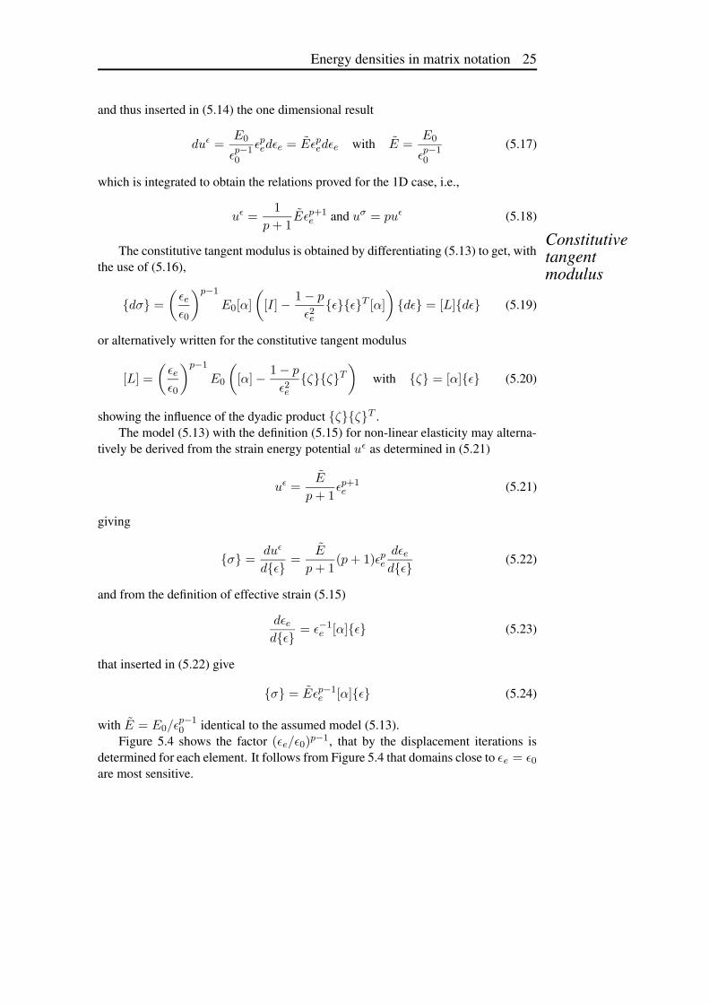
with E = E0/εp−10 identical to the assumed model (5.13).
Figure 5.4 shows the factor (εe/ε0)p−1, that by the displacement iterations is
determined for each element. It follows from Figure 5.4 that domains close to εe = ε0
are most sensitive.
26 c©Pauli Pedersen: Stationarity and extremum principles in mechanics
0
0.2
0.4
0.6
0.8
1
0 0.05 0.1 0.15 0.2 0.25 0.3 0.35 0.4
PSfrag replacements
εe
(
εe
ε0
)p−1
p = 0.9
p = 0.8
p = 0.6
p = 0.4
p = 0.2
p = 0.1
Figure 5.4: Illustration of the stiffness factor (εe/ε0)p−1 as function of the effective strain
εe.
5.4 Summing up• The notations uε for strain energy density and uσ for stress energy density are
chosen as alternative to the use of complementary energy density in order tofocus on the relational dependence.
• The sum of these energy densities is denoted φ and only for linear elasticity isuε = uσ = 1
2(uε + uσ) = 12φ.
• However, for all non linear elasticity is φ = uε + uσ.
• For power law non linear elasticity with power p is uσ = puε, and secant aswell as tangent constitutive matrices are analytical available.
• Note the misprint in the references (Pedersen 2005a), (Pedersen 2005b), and(Pedersen 2006), where in formulas corresponding to 5.19 the denominator ε2
e
for Green-Lagrange strains is written η2ref and should be η2
eff , as here and inthe early reference (Pedersen and Taylor 1993).
Chapter 6
Elastic energy in beam models
6.1 Elastic energy in a straight beamIn handbooks of strength of materials, like in (Sundstrøm 1998), we find the formulafor elastic energy (based on linear, isotropic elasticity) in a straight beam of lengthb − a Handbook
formulasU ε = Uσ = UσN + UσT + UσM + UσMx
=
∫ b
a
(
N2
2EA+ β
T 2
2GA+
M2
2EI+
M2x
2GK
)
dx (6.1)
where the cross-sectional forces/moments are
N = normal force, T = transverse(shear) forceM = bending moment, Mx = torsional moment
The material parameters of the assumed isotropic linear elastic behaviour are
E = Young’s modulus, ν = Poisson’s ratio
G = shear modulus =E
2(1 + ν)
and the cross-sectional constants are
A = area (tension/compression stiffness factor)I = moment of inertia (bending stiffness factor)K = torsional stiffness factorβ = factor from the shear stress distribution
Let us primarily prove the individual terms in (6.1) based on the definitions inChapter 2. With only a normal force N and stresses uniformly distributed over thecross-section we get Normal
forceσ =
N
A, ε =
σ
E, uε = uσ =
σε
2=
σ2
2E=
ε2E
2
⇒ uε = uσ =N2
2A2E(6.2)
27
28 c©Pauli Pedersen: Stationarity and extremum principles in mechanics
With uniformly distributed energy density, the energy per length is uσA = N2/(2EA)as stated in (6.1).
With only a bending moment M the stresses vary linearly through the height hof the beam
Bendingmoment
σ =Mz
I, for −h
2≤ z ≤ h
2
⇒ uε = uσ =M2z2
2I2E(6.3)
and with the moment of inertia defined by I =∫
A z2dA, the energy per length is∫
A uσdA = M2/(2EI) as stated in (6.1).After the two cases of pure normal stress let us analyze the case of only a trans-
verse force T . The distribution of shear stresses τ = τ(z) (τ = σ12) will depend onthe specific cross-sectional shape, and is here stated as
τ = τmaxf(z) with f(z) = 0 for z = ±h
2(6.4)
Then with engineering shear strain γ = 2ε12 and µ as a cross-sectional constant,determined by a function f(z), the analog to (6.2) isTransverse
forceτmax =
µT
A, τ = τmaxf(z), γ =
τ
G, uε = uσ =
τγ
2=
τ2
2G=
γ2G
2
⇒ uε = uσ =µ2T 2
2A2Gf2(z) (6.5)
Integrating to energy per length∫
A uσdA, we see that the constant β in (6.1) must bedefined by
β =
(∫
Af2(z)dA
)
µ2
A(6.6)
For specific values of µ, β, see (Sundstrøm 1998) or an alternative handbook.Finally the case of only a torsional moment, here restricted to circular cross-
sections for which the stress distribution with outer radius R isTorsionalmoment
τmax =MxR
K, τ =
τmaxr
R=
Mxr
Kfor rmin ≤ r ≤ R
(6.7)
In analog to (6.5) we then get
uε = uσ =τ2
2G=
M2xr2
2K2G(6.8)
which with K =∫
A r2dA for circular cross-sections gives the energy per length asstated in (6.1). The non-circular cross-sections is not covered here.
Energy is not linear in stresses as seen from (6.1), where N , T , M and Mx areoften termed generalized stresses. We therefore need to prove that the simple additionof the four energies is correct. For the normal stresses with both N and M we getDecoupled
energiesσ =
N
A+
Mz
I⇒ σ2 =
N2
A2+
M2z2
I2+
2NMz
AI(6.9)
Elastic energy in beam models 29
and the last term will not give rise to energy because by definition of the beam axiswe have
∫
A zdA = 0.For the shear stresses with both T and Mx it is more simple to look at the work
of T and Mx instead of the elastic energy and then base the proof on the energyprinciples of Chapter 2. The beam displacements from T give no rotation around thebeam length direction and therefore no work by Mx. Similar the beam cross-sectionalrotation from Mx give no transverse displacement and therefore no work by T . Thusthe decoupling’s in (6.1) are correct.
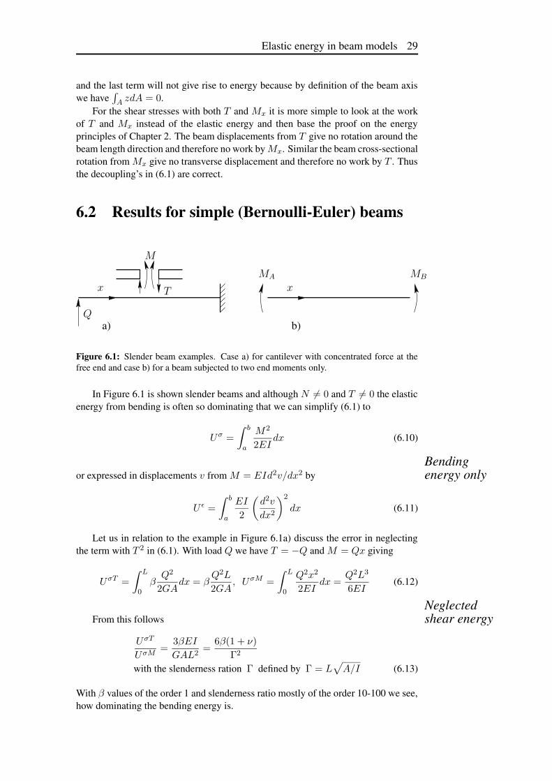
6.2 Results for simple (Bernoulli-Euler) beamsPSfrag replacements
Q
T
M
xx
a)
MA MB
b)
Figure 6.1: Slender beam examples. Case a) for cantilever with concentrated force at thefree end and case b) for a beam subjected to two end moments only.
In Figure 6.1 is shown slender beams and although N 6= 0 and T 6= 0 the elasticenergy from bending is often so dominating that we can simplify (6.1) to
Uσ =
∫ b
a
M2
2EIdx (6.10)
Bendingenergy onlyor expressed in displacements v from M = EId2v/dx2 by
U ε =
∫ b
a
EI
2
(
d2v
dx2
)2
dx (6.11)
Let us in relation to the example in Figure 6.1a) discuss the error in neglectingthe term with T 2 in (6.1). With load Q we have T = −Q and M = Qx giving
UσT =
∫ L
0β
Q2
2GAdx = β
Q2L
2GA, UσM =
∫ L
0
Q2x2
2EIdx =
Q2L3
6EI(6.12)
Neglectedshear energyFrom this follows
UσT
UσM=
3βEI
GAL2=
6β(1 + ν)
Γ2
with the slenderness ration Γ defined by Γ = L√
A/I (6.13)
With β values of the order 1 and slenderness ratio mostly of the order 10-100 we see,how dominating the bending energy is.
30 c©Pauli Pedersen: Stationarity and extremum principles in mechanics
The important case of linearly varying moment shown in Figure 6.1b) give M(x) =MA +(MB −MA)x/L and then from (6.10) with constant bending stiffness EI give
Uσ =1
2EI
∫ L
0
(
MA + (MB − MA)x
L
)2dx =
L
6EI(M2
A + M2B + MAMB)
(6.14)which could have given (6.12) directly for MA = QL and MB = 0.Elementary
case6.3 Beam solutions by stress(complementary)
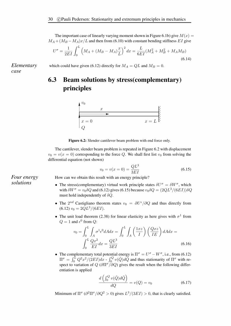
principlesPSfrag replacements
x
Q
v0
x = 0 x = L
Figure 6.2: Slender cantilever beam problem with end force only.
The cantilever, slender beam problem is repeated in Figure 6.2 with displacementv0 = v(x = 0) corresponding to the force Q. We shall first list v0 from solving thedifferential equation (not shown)
v0 = v(x = 0) =QL3
3EI(6.15)
How can we obtain this result with an energy principle?Four energysolutions • The stress(complementary) virtual work principle states δU σ = δW σ, which
with δW σ = v0δQ and (6.12) gives (6.15) because v0δQ = (2QL3/(6EI))δQmust hold independently of δQ.
• The 2nd Castigliano theorem states v0 = ∂U ε/∂Q and thus directly from(6.12) v0 = 2QL3/(6EI).
• The unit load theorem (2.38) for linear elasticity as here gives with σ1 fromQ = 1 and ε0 from Q:
v0 =
∫ L
0
∫
Aσ1ε0dAdx =
∫ L
0
∫
A
(
1xz
I
)(
Qxz
IE
)
dAdx =
∫ L
0
Qx2
EIdx =
QL3
3EI(6.16)
• The complementary total potential energy is Πσ = Uσ −W σ, i.e., from (6.12)Πσ =
∫ L0 Q2x2/(2EI)dx -
∫ Q0 v(Q)dQ and thus stationarity of Πσ with re-
spect to variation of Q (∂Πσ/∂Q) gives the result when the following differ-entiation is applied
d(
∫ Q0 v(Q)dQ
)
dQ= v(Q) = v0 (6.17)
Minimum of Πσ (∂2Πσ/∂Q2 > 0) gives L3/(3EI) > 0, that is clearly satisfied.

Elastic energy in beam models 31
6.4 Summing up• The elastic energy in a straight beam of linear, isotropic, homogeneous mate-
rial is integrated along the beam axis, that contains the centers of cross sec-tional gravity. The formula 6.1 is taken from a handbook.
• Although energy is not linear in the cross sectional forces and moments, thesimple addition from each of these is proved.
• The coefficient β to the shear force component must be determined by inte-gration for a specific cross section.
• As an example four different energy principles are shown to give the sameresult.

32 c©Pauli Pedersen: Stationarity and extremum principles in mechanics
Chapter 7
Some necessary conditions foroptimality
In this chapter we primarily present two necessary conditions for optimal solutionsin general, i.e. not directly related to optimal design. The first condition is only valid General
optimizationfor non-constrained problems and the second condition is valid for problems withonly a single constraint in addition to the objective.
After the two first sections we then determine, expressed in physical terms, thecondition for solution of the most simple optimal design problems, for which sizes(or field of size) optimize stiffness as well as strength. The optimal designs to thesetwo different problems are shown to be the same. Design
optimizationIn close relation to the analysis for size optimization, we treat optimization ofshape, again to optimize stiffness as well as strength. The shape solution to these twodifferent problems is shown in many cases also to be the same, very much in parallelto the result for size optimization. Size and
shapeA simple parametrization for shape optimization is finally described. The goalof the present chapter is to obtain basic understanding of very simple optimal designproblems, without involving extended numerical calculations.
7.1 Non-constrained problemsThe notion of Φ is often used for compliance as in (2.13), but in Sections 7.1 and 7.2it is applied for a more general objective. A non-constrained optimization problemmay be defined as
Extremize Φ = Φ(he) with variables he non-constrained (7.1)
and a necessary condition for this is that the objective Φ is stationary with respect to Stationaryobjectiveall the independent variables he
dΦ/dhe = 0 for all e (7.2)
The optimization of material orientation is an important example of such a non-constrained problem. Unfortunately, this problem is not simple to solve, becausemany local optima exist. Each variable (orientational angle θe in a domain e) hasseveral solutions to the stationarity condition (7.2).
33
34 c©Pauli Pedersen: Stationarity and extremum principles in mechanics
7.2 Problems with a single constraintAn optimization problem with only a single constraint may be defined as
Extremize Φ = Φ(he) with variables he
constrained by g = g(he) = 0 (7.3)
To obtain an optimality condition we convert this problem to a non-constrained prob-Convertedto non-constrained
lem, using a Lagrangian function L = Φ − λg to be made stationary for arbitraryvalue of λ (the Lagrangian multiplier). It follows from (7.2) that a necessary opti-mality condition is
dL/dhe = 0 for all e ⇒dΦ/dhe = λdg/dhe (7.4)
This general result we read as proportionality between the gradient of the objec-Proportionalgradients tive and the gradient of the single constraint. The factor of proportionality, the La-
grangian multiplier λ, is determined by the constraint condition g(he) = 0, thatfollows from dL/dλ = −g = 0.
The use of the optimality condition (7.4) for obtaining more general informationabout optimal design is very important. It should be noted that behind this result isthe assumption that the constraint is active. Extensions to two and more constraintsare possible, but the uncertainty about the active constraints is then often a limitingfactor on the usefulness.
An alternative look at the problem is to postulate (7.4) and then see that dg = 0implies dΦ = 0, i.e.
dΦ =∑
e
∂Φ
∂he∆he = λ
∑
e
∂g
∂he∆he = λdg = 0 (7.5)
7.3 Size optimization for stiffness and strengthThe theoretical results for size optimization are more developed than those for shapeoptimization. Let us therefore start with some basis knowledge from size optimiza-tion, as it can be found in (Pedersen 1998b) for non-linear elasticity or in (Wasiutyn-ski 1960) for linear elasticity.
7.3.1 Size design with optimal stiffnessIf the objective is to minimize compliance (minimize elastic energy) for given totalmass then we have (for optimal stiffness design with homogeneous assumptions andHomogeneous
mass(volume)dependence
design independent loads): the ratio between sub-domain energy and sub-domainmass should be the same in all the design sub-domains.
Let the design parameters be he, then homogeneous mass relations are obtainedwith M =
∑
e Me =∑
e hme Me, where M is the total mass, Me is the mass in do-
main e, m is a given positive value, and Me is independent of the design parameters.The homogeneous energy relations are obtained with Uε =
∑
e Uεe =∑
e hne Uεe ,
where Uε is the total strain energy, Uεe is the strain energy in domain e, n is a givenpositive value, and Uεe is explicitly independent of the design parameters.
Restricted to problems with constant mass density we get, in all design domains,the same mean strain energy density. Furthermore, if the model has constant energy
Some necessary conditions for optimality 35
density within a design domain, then the result for the optimal design is uniformstrain energy density u∗
ε , i.e.
u∗εe
= uε for all free design domains (7.6)
where lower and upper size constraints are not reached. The symbolism here is Stiffestdesigna super-index ∗ related to the optimal design, and a overhead bar ¯ indicating a
constant value for each domain e (mean value).Assume now that the necessary condition (7.6) give a global minimum solution,
then for any other design the total strain energy Uε is larger (or equal to)
Uε =∑
e
uεeVe ≥ U∗ε =
∑
e
u∗εV
∗e = uε
∑
e
V ∗e = uε
∑
e
Ve =∑
e
u∗εe
Ve (7.7)
where V ∗e is the optimal volume of the design domain e. For an alternative design
with design volumes Ve we have the same total volume V V =∑
e Ve =∑
e V ∗e .
From (7.7) we get∑
e
(uεe − u∗εe
)Ve ≥ 0 (7.8)
7.3.2 Size design with optimal strengthAlso beststrengthWith positive volumes Ve we read from (7.8), that at least one uεe is not less than u∗
εe.
Thus if the strongest design is defined by minimum of maximum uεe , then the stiffestdesign characterized by the optimality condition (7.6) is also the strongest design.
We note that the strength may also be defined in relation to the von Mises stressor an alternative effective stress, and these measures are not always proportional tothe energy density. For a detailed discussion of these aspects see (Pedersen 1998b).
7.4 Shape optimization for stiffness and strengthIn the following we use the same kind of reasoning to draw conclusions about shapeoptimization, without involving a solution to the actual stress problem. Thus wegain general knowledge, valuable for 3D and 2D-problems, for non-linear elastic as General
knowledgewell as for linear problems, for non-isotropic or isotropic problems, for any external,design independent load. Also valid for non-homogeneous problems and independentof the solution procedure.
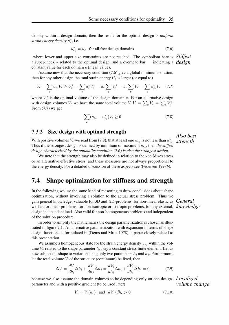
In order to simplify the mathematics the design parametrization is chosen as illus-trated in figure 7.1. An alternative parametrization with expansion in terms of shapedesign functions is formulated in (Dems and Mroz 1978), a paper closely related tothis presentation.
We assume a homogeneous state for the strain energy density uεe within the vol-ume Ve related to the shape parameter he, say a constant stress finite element. Let usnow subject the shape to variation using only two parameters hi and hj . Furthermore,let the total volume V of the structure (continuum) be fixed, then
∆V =dV
dhi∆hi +
dV
dhj∆hj =
dVi
dhi∆hi +
dVj
dhj∆hj = 0 (7.9)
because we also assume the domain volumes to be depending only on one design Localizedvolume changeparameter and with a positive gradient (to be used later)
Ve = Ve(he) and dVe/dhe > 0 (7.10)
36 c©Pauli Pedersen: Stationarity and extremum principles in mechanics
Figure 7.1: Discretized design parametrization, showing two design domains i and j.
7.4.1 Shape design with optimal stiffnessIn shape optimization for extremum elastic strain energy the increment of the objec-tive corresponding to increments ∆hi, ∆hj is
∆Uε =dUε
dhi∆hi +
dUε
dhj∆hj (7.11)
which for power law non-linear elasticity σ = Eεp can be written asDesignindependentloads ∆Uε = −1
p
(
∂Uε
∂hi∆hi +
∂Uε
∂hj∆hj
)
fixed strains(7.12)
This is proved in (Pedersen 1998b) for design independent loads, and followsfrom (4.10) in chapter 4. Therefore only the local energies Uεi
= uεiVi and Uεj
=uεj
Vj are involved and the variations in the strain energy densities need not be deter-mined, because the constitutive relations are unchanged. We haveLocalized
energychange ∆Uε = −1
p(uεi
dVi
dhi∆hi + uεj
dVj
dhj∆hj) (7.13)
and inserting (7.9) in (7.13) we obtain
∆Uε = −1
p(uεi
− uεj)dVi
dhi∆hi (7.14)
A necessary condition for optimality ∆Uε = 0 with dVi/dhi > 0 is thereforeuεi
= uεj.
With all design parameters, eq. (7.9) and (7.13) are written
∆V =∑
e
dVe
dhe∆he
∆Uε = −1
p
∑
e
uεe
dVe
dhe∆he (7.15)
and we conclude that a necessary condition for optimality ∆U = 0 with constraint∆V = 0 is constant strain energy density uεe . Thus for the stiffest design the energydensity along the shape(s) to be designed, here denoted uεs , must be constantConstant
energydensity uεs = uε (7.16)

Some necessary conditions for optimality 37
7.4.2 Shape design with optimal strengthWe now relate the stiffest design (minimum compliance) to the strongest design (min-imum maximum strain energy density). Let us assume that the highest strain energydensity is at the shape to be designed. With index s referring to shape design domainsand index n referring to domains not subjected to design changes, this means that forthe stiffest design we assume
uεs = uε > uεn (7.17)
A design domain that depends on design parameter is given index s (hs) and a design Basicassumptiondomain which is not subjected to design change is given index n (hn). For the total
design domain we use index S and for the total domain not subjected to design, indexN . The total elastic strain energy Uε is obtained from
Uε = UεS+ UεN
=∑
s
Uεs +∑
n
Uεn =∑
s
uεsVs +∑
n
uεnVn ,i.e.,
Uε = uε
∑
s
Vs +∑
n
uεnVn (7.18)
With unchanged domain N and for the stiffest design Uε > U∗ε we obtain
∑
s
uεsVs +∑
n
uεnVn >∑
s
uεV∗s +
∑
n
u∗εn
V ∗n ,i.e.,
∑
s
(uεs − uε)Vs >∑
n
(u∗εn
− uεn)Vn (7.19)
as∑
s uεV∗s =
∑
s uεVs due to given total volume, and furthermore individual un-changed in the non-design domains V ∗
n = Vn.The right hand side might be negative, so we can not directly draw conclusions
as from (7.8). However, in a complementary formulation with stress energies we canprove that the right hand side is non-negative and then the proof holds.
The proof of increasing energy in the shape domain is as follows. We write the Detail ofprooftotal stress energy Uσ as the sum of stress energy in the shape domain UσS
and stressenergy in the non-shape domain UσN
and obtain
Uσ = UσS+ UσN
⇒ dUσ
dh=
dUσS
dh+
dUσN
dh(7.20)
From the principle of complementary virtual work followsdUσ/dh = (∂Uσ/∂h)fixed stress field and we get
dUσ
dh=
(
∂UσS
∂h+
∂UσN
∂h
)
fixed stress field(7.21)
where the last term is zero when h has no direct influence on the non-shape domain.Finally for the stiffest design we have dUσ/dh > 0 and from this we conclude
(
∂UσS
∂h
)
fixed stress field=
dUσ
dh=
1
p
dUεS
dh> 0 (7.22)
Summarizing the theoretical results of this section; we have for the general three-dimensional case with non-isotropic, power law non-linear elastic material in an non-homogeneous structure, and for any design independent single load case that:
38 c©Pauli Pedersen: Stationarity and extremum principles in mechanics
The minimum compliance shape design (stiffest shape design) has uniform energydensity along the designed shape, as far as the geometrical constraints make thispossible.
If we furthermore assume that the highest energy densities are found at the de-signed shape, then the stiffest design is also the strongest design, as defined by adesign which minimizes the maximum energy density.Design for
stiffnessand strength
Note that these results are obtained without calculating the stress/strain fields andwithout specifying the constitutive behaviour. This behaviour need not be homoge-neous and thus we can also include the multi-material case.
7.5 Conditions with asimple shape parametrization
In the final conclusions in section 7.4.2, we have added the note ”as far as the geo-metrical constraints make this possible”. Also it was commented that normally theshape parametrization implies such a geometrical constraint. In this section we usea simple shape parametrization that makes a rather simple optimality condition pos-sible. The limitations of using this simple parametrization can be evaluated by thepossibility to obtain almost uniform energy density distribution along the shape to beGood
experience designed. Many examples illustrate that the parametrization is in fact able to describeoptimal shapes in many cases.
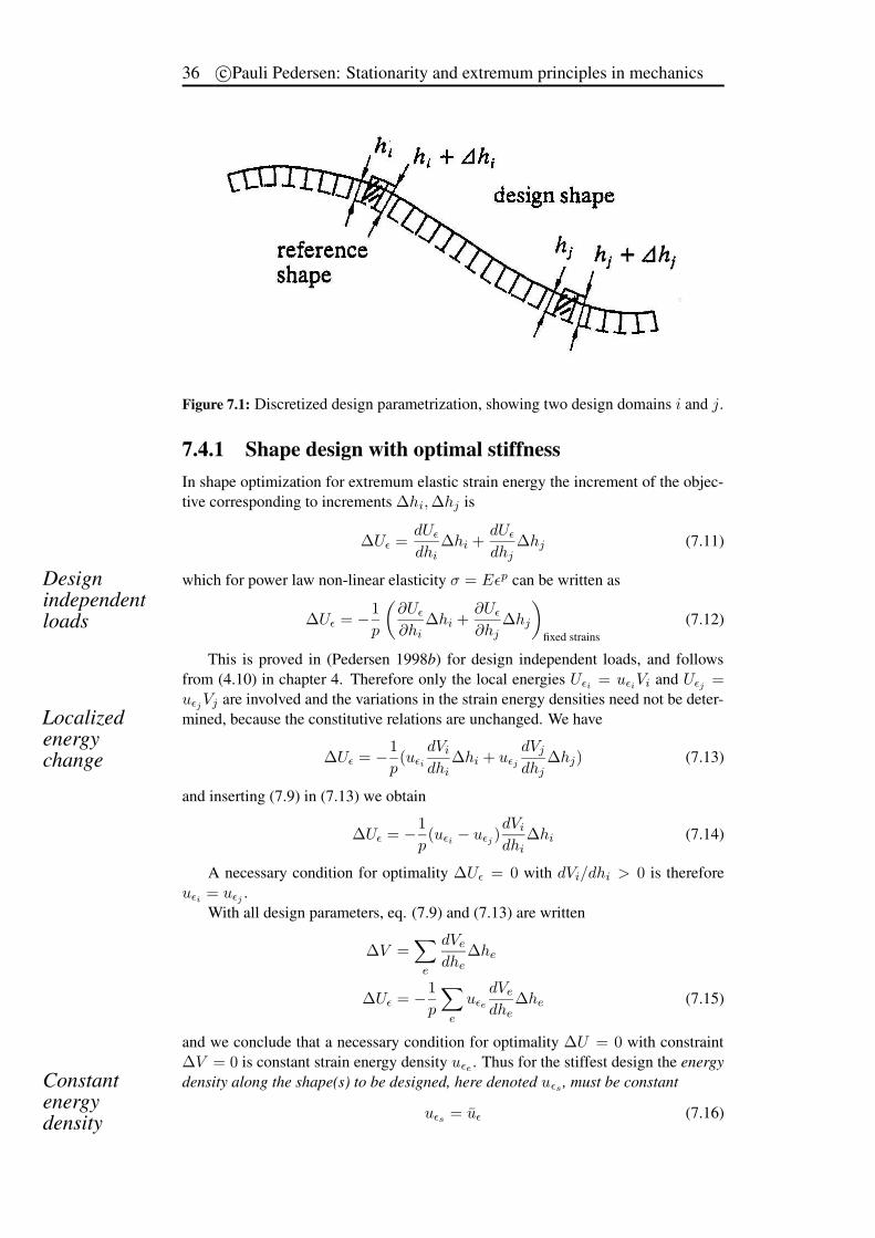
Figure 7.2: A three parameter (α, β, η) description of an internal hole in a rectangulardomain, specified by A, B.
Figure 7.2 shows a single inclusion hole, where the shape of the boundary is mod-eled as a super-elliptic shape, described by only three non-dimensional parameters,relative axes α, β and power η
( x
αA
)η+
(
y
βB
)η
= 1 (7.23)
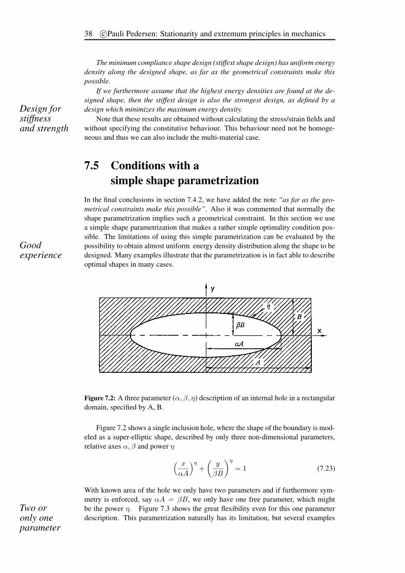
With known area of the hole we only have two parameters and if furthermore sym-metry is enforced, say αA = βB, we only have one free parameter, which mightbe the power η. Figure 7.3 shows the great flexibility even for this one parameterTwo or
only oneparameter
description. This parametrization naturally has its limitation, but several examples
Some necessary conditions for optimality 39
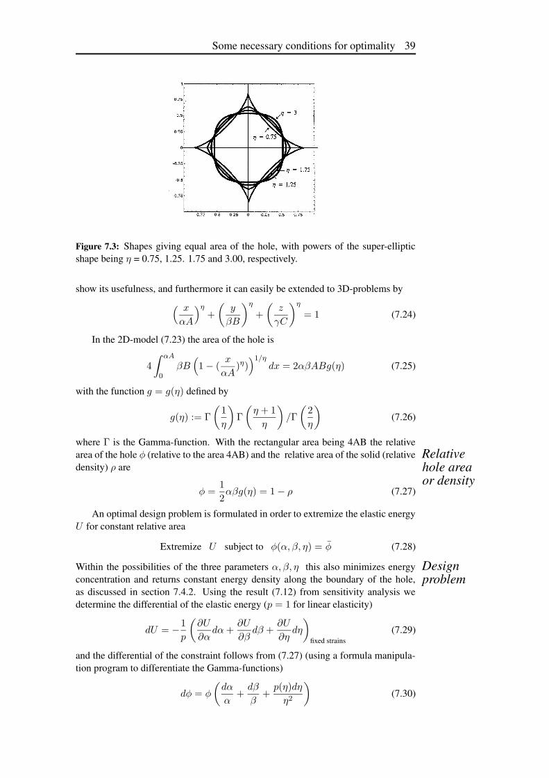
Figure 7.3: Shapes giving equal area of the hole, with powers of the super-ellipticshape being η = 0.75, 1.25. 1.75 and 3.00, respectively.
show its usefulness, and furthermore it can easily be extended to 3D-problems by( x
αA
)η+
(
y
βB
)η
+
(
z
γC
)η
= 1 (7.24)
In the 2D-model (7.23) the area of the hole is
4
∫ αA
0βB
(
1 − (x
αA)η))1/η
dx = 2αβABg(η) (7.25)
with the function g = g(η) defined by
g(η) := Γ
(
1
η
)
Γ
(
η + 1
η
)
/Γ
(
2
η
)
(7.26)
where Γ is the Gamma-function. With the rectangular area being 4AB the relativearea of the hole φ (relative to the area 4AB) and the relative area of the solid (relative Relative
hole areaor density
density) ρ are
φ =1
2αβg(η) = 1 − ρ (7.27)
An optimal design problem is formulated in order to extremize the elastic energyU for constant relative area
Extremize U subject to φ(α, β, η) = φ (7.28)
Within the possibilities of the three parameters α, β, η this also minimizes energy Designproblemconcentration and returns constant energy density along the boundary of the hole,
as discussed in section 7.4.2. Using the result (7.12) from sensitivity analysis wedetermine the differential of the elastic energy (p = 1 for linear elasticity)
dU = −1
p
(
∂U
∂αdα +
∂U
∂βdβ +
∂U
∂ηdη
)
fixed strains(7.29)
and the differential of the constraint follows from (7.27) (using a formula manipula-tion program to differentiate the Gamma-functions)
dφ = φ
(
dα
α+
dβ
β+
p(η)dη
η2
)
(7.30)

40 c©Pauli Pedersen: Stationarity and extremum principles in mechanics
with the function p = p(η) defined by
p(η) := Ψ
(
2
η
)
− Ψ
(
1
η
)
− Ψ
(
η + 1
η
)
(7.31)
where Ψ is the Psi-function. To illustrate that the functions g(η) and p(η) are well-Availablefunctions behaved functions we show in figure 7.4 these functions and there derivatives. These
functions are available in many libraries of computer routines.
Figure 7.4: Left g-function and right the p-function with their derivatives as a functionof the shape power η.
The condition of dU = 0 when dφ = 0 is a necessary condition for optimalityand thus (as in general with only a single constraint) we from (7.29) and (7.30) getthe optimality condition by proportional gradients (7.4), i.e.Optimality
condition(
α∂U
∂α= β
∂U
∂β=
η2
p(η)
∂U
∂η
)
fixed strains(7.32)
In a fixed strain field the energy densities u are constant and only the volumes ofdomains (elements) connected to the hole boundary change. Thus in a finite elementFor model
by the FEM formulation the optimality condition (7.32) is written
α∑
s
us∂Vs
∂α= β
∑
s
us∂Vs
∂β=
η2
p(η)
∑
s
us∂Vs
∂η(7.33)
where index s refers to an element connected to the hole boundary. The only infor-mation needed in addition to the results from analysis is ∂Vs/∂α, ∂Vs/∂β, ∂Vs/∂η,i.e. only information from geometry. We note, in agreement with section 7.4.2, thatif us is constant along the hole boundary then
∑
s ∂Vs/∂α = ∂V/∂α = φ/α etc.,and the optimality criterion (7.33) is satisfied by usφ = usφ = usφ. Thus a con-stant energy density along the boundary of the hole implies stationary total elasticStrength or
stiffness energy. However, we can have stationary energy without constant energy density, ifthe possible designs are restricted. This is illustrated by the examples in chapter ??.
7.5.1 Possible iterative procedureThe problem is how to find a boundary shape that satisfies (7.32) or in finite ele-ment formulation (7.33). The heuristic approach of successive iterations could be toestimate the Lagrange multiplier λ by the mean value
λestimated =1
3
(
α∂U
∂α+ β
∂U
∂β+
η2
p(η)
∂U
∂η
)
(7.34)
Some necessary conditions for optimality 41
and then redefine α, β, η by
αnew = λ/(∂U
∂α)old, βnew = λ/(
∂U
∂β)old, (
η2
p(η))new = λ/(
∂U
∂η)old (7.35)
with iterations on λ to satisfy the constraint of (7.28) Estimatedmultiplier
φnew =1
2αnewβnewg(ηnew) = φ (7.36)
7.6 Summing upIn this chapter the important results to focus on are: Collected
results• For non-constrained problems the necessary optimality condition is stationar-
ity of the objective with respect to all the independent variables.
• For problems with a single constraint the necessary optimality condition isproportionality between the gradient of the objective and the gradient of thesingle constraint.
• For size optimization of stiffness and strength the stiffest design is character-ized by the optimality condition of uniform energy density and this design isalso the strongest design.
• For shape optimization of stiffness, the minimum compliance shape design(stiffest shape design) has uniform energy density along the designed shape,as far as the geometrical constraints make this possible.
• For shape optimization of strength, if we assume that the highest energy den-sities are found at the designed shape, then the strongest design, as definedby a design which minimizes the maximum energy density, is also the stiffestdesign.
• For shape optimization a simple super-elliptic description makes it possible todesign a wide spectrum of shapes, and the analytical treatment of this case isalmost as simple as the classic elliptic case.
• The super-elliptic description can be extended to include a skewness param-eter, and then also describe triangular shapes, see (Pedersen 2004) for moredetail.

42 c©Pauli Pedersen: Stationarity and extremum principles in mechanics
Chapter 8
Analytical beam designStaticallydeterminatebeams
Beams are among the most important structural elements with classical results foranalysis as well as for design. Especially the statically determinate cases constitute abasic knowledge in solid mechanics, treated in a one dimensional formulation. Thepresent chapter originates from a study published in (Pedersen and Pedersen 2008)and describes the general aspects from an energy point of view, but only the mostsimple examples of the statically determinate beams are included. Analytical
stepsThe analytical approach has two steps, first determining analytically the neces-sary optimality criterion as it is often found in the literature; for early reference oncompliance minimization see (Huang 1968) and (Masur 1970). Second analyticalstep is to determine an explicit analytical solution to the optimality criterion and thisstep is limited to statically determinate beams as the optimality criterion can then bewritten independent of design. The problems of the present chapter are chosen sothat a full analytical approach is reasonable.
For long beams (Bernoulli-Euler beams) a number of optimal designs are analyt-ically described as refereed in (Save, Prager and Sacchi 1985) and (Rozvany 1989),with most focus on designs based on plastic collapse. These problems may be for-mulated to maximize stiffness or maximize eigenfrequency for a given amount ofmaterial volume or mass, see the review (Olhoff and Taylor 1983). The solutions de-pend on the actual boundary conditions and load conditions in addition to the chosendesign type, i.e., the chosen relation between cross sectional area and cross sectionalmoment of inertia. Bernoulli-Euler beam theory is applied in most treated cases , andlittle analytical attention is given to short beams for which Timoshenko beam theoryis necessary. Timoshenko
beam theoryIn short beam structures the elastic energy from shear forces can not be neglected.From a practical point-of-view more realistic designs are obtained when this addi-tional energy is taken into account, but only a few optimal designs with analyticaldescription are then available. The goal of the present chapter is to present suchresults from (Pedersen and Pedersen 2008).
Primarily, the statics of some statically determinate cases are presented withone dimensional distribution of shear force T = T (x) and of bending momentM = M(x). Material is assumed isotropic and when the beam has cross sectionaldistribution of area A = A(x) and cross sectional moment of inertia I = I(x), thenthe distribution of elastic energy per unit length is given. In beams the cross sectionalmoment of inertia I = I(x) plays a major role and thus we need a relation betweenarea and moment of inertia. Three possibilities are treated in the present chapterwith I(x) proportional to A(x), to A2(x), or to A3(x). The cross sectional types
43
44 c©Pauli Pedersen: Stationarity and extremum principles in mechanics
specifically treated in the present chapter are limited to those presented in Section8.4. To illustrate the influence of beam length on the design, the common expressionCross sectional
size I(x) = CAn(x) is further specified as C = γb2(2−n) with γ as a non-dimensionalconstant in the range 0.08 ≤ γ ≤ 0.25 for the treated cases. Beam length L isgiven relative to a cross sectional length parameter b, i.e., L = ηb, treating η as anon-dimensional length parameter.Beam length
In optimal design formulation for minimum compliance with point wise designvariables, a necessary optimality criterion is uniform elastic energy density. In beamdesign with the cross sectional area A = A(x) as design parameter the optimalitycriterion must be stated for this two dimensional design domain. The gradient ofthe elastic energy per unit length with respect to area change, must as a necessarycondition be the same for all areas, i.e., at all positions x. For the simplest cases, i.e.,all Bernoulli-Euler beams and Timoshenko beams with I(x) linearly depending onA(x) this means that the mean value of elastic energy density should be the same forall areas. However, this later statement of the optimality criterion is not valid for allTimoshenko beams.
Four cases of statically determinate beams are analyzed in (Pedersen and Ped-ersen 2008): Bernoulli-Euler cantilevers, Bernoulli-Euler simply supported, Timo-shenko cantilevers, and Timoshenko simply supported. For each of these four beammodels three load cases are applied, and in addition to the cross sectional parametern = 1, 2, 3 in An(x), this adds up to 36 individual cases. As examples in the presentchapter are only presented the cantilever beams.Use of optimal
design results In two and three dimensional design of beam like structures, this knowledge onA∗(x) can be used to compare with numerically obtained results or as initial designs.The presented values of compliance decrease also give possibility for comparing withalternatively obtained results.
8.1 Optimality criterion for beam designThe optimization problem is stated as
Minimize compliance Φ
for a given volume V =
∫ L
0A(x)dx (8.1)
where the cross sectional area A(x) is integrated along the beam axis x from 0 tolength L. The length is specified relative to a cross sectional reference length b asL = ηb with the influence of the non-dimensional parameter η, for short beamsshowed in the range 1 ≤ η ≤ 5. The area function A(x) is the design function to beoptimized, then denoted A∗(x).
The compliance Φ is the work of external dead loads and may be evaluated as thesum of internal elastic energies (stress energy + strain energy) Φ = Uσ + Uε. Usingbeam theory under the assumption of zero normal force and zero torsional moment(with linear elasticity Φ = 2Uσ = 2Uε) the compliance isCompliance
objectiveΦ =
∫ L
0φ(x)dx with φ(x) = β
T 2(x)
GA(x)+
M2(x)
EI(x)(8.2)
where φ(x) is twice the stress elastic energy per unit length, T (x) the shear force,M(x) the bending moment, I(x) the cross sectional moment of inertia, G the shear
Analytical beam designs 45
modulus, and E Young’s modulus. For isotropic material we have G determined byPoisson’s ratio ν as E = 2(1 + ν)G. The factor from the cross sectional distributionof shear stresses is β, here approximated to be unchanged along the beam, and beingin the range 1 < β < 2.
In Section 8.4 different models of type I(x) = CAn(x) are shown, with values ofthe power n = 1, 2, 3 and correspondingly different dimensions of the quantity C thatdoes not depend on the actual design variable. Introducing the model C = γb2(2−n)
give Model formoment ofinertiaI(x) = γb2(2−n)An(x) for n = 1, 2, or 3 (8.3)
where b is a cross sectional reference length, assumed constant for the optimization.Section 8.4 shows examples where for n = 1 the size b is the width w or the heighth with 1
12 ≤ γ ≤ 14 . For n = 2 the size b disappear in (8.3) and as reference value
b a kind of mean value√
V/L may be chosen, for this case 14π ≤ γ ≤
√3
18 . Finallyfor n = 3 the size b is again the width w and γ = 1
12 . Totally the non-dimensionalparameter γ is in the range 0.08 ≤ γ ≤ 0.25 for the cases shown in Section 8.4.
Twice the stress elastic energy per unit length, (8.2) and (8.3) is
φ(x) =1
γE
(
αT 2(x)
A(x)+
M2(x)b2n
b4An(x)
)
with α = 2γβ(1 + ν) (8.4)
For practical cases the defined non-dimensional parameter α is of the order 1. Witha non-dimensional parenthesis and a design independent factor, then (8.4) is written Compliance
per unitlengthφ(x) =
Q2
γEb2
(
α(T (x)/Q)2
A(x)/b2+
(M(x)/(Qb))2
(A(x)/b2)n
)
with α = 2γβ(1 + ν) (8.5)
where Q is the total external force. The shear force distribution T (x) and the momentdistribution M(x) are independent of design for statically determinate cases.
The optimality condition for an objective with a single active constraint is givenby proportional gradients, as stated in (7.4). For the compliance problem (8.1) withA(x) as design parameter and λ as a positive constant this give
dΦ
dA(x)=
∫ L
0
dφ(x)
dA(x)dx = −λ
dV
dA(x)= −λ
∫ L
01dx or
∫ L
0
(
dφ(x)
dA(x)+ λ
)
dx = 0 (8.6)
to hold for any variation of A(x). For the statically determinate cases only A(x) in(8.4) is varying and differentiation gives
dφ(x)
dA(x)=
1
γE
(
−αT 2(x)
A2(x)− n
M2(x)b2n
b4An+1(x)
)
(8.7)
and the necessary condition (8.6) to hold at all x may be expressed by a new non-dimensional positive constant λ, defined by Optimality
criterionλ = α
(T (x)/Q)2
(A∗(x)/b2)2+ n
(M(x)/(Qb))2(A∗(x)/b2)n+1
(8.8)
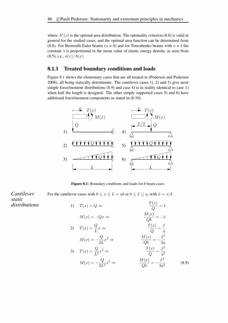
46 c©Pauli Pedersen: Stationarity and extremum principles in mechanics
where A∗(x) is the optimal area distribution. The optimality criterion (8.8) is valid ingeneral for the studied cases, and the optimal area function can be determined from(8.8). For Bernoulli-Euler beams (α = 0) and for Timoshenko beams with n = 1 theconstant λ is proportional to the mean value of elastic energy density, as seen from(8.5), i.e., φ(x)/A(x).
8.1.1 Treated boundary conditions and loadsFigure 8.1 shows the elementary cases that are all treated in (Pedersen and Pedersen2008), all being statically determinate. The cantilever cases 1), 2) and 3) give mostsimple force/moment distributions (8.9) and case 4) is in reality identical to case 1)when half the length is designed. The other simply supported cases 5) and 6) haveadditional force/moment components as stated in (8.10).
PSfrag replacementsxx
LL
1)
2)
3)
4)
5)
6)
L/2
T (x)T (x)
M(x) M(x)
Figure 8.1: Boundary conditions and loads for 6 beam cases.
For the cantilever cases with 0 ≤ x ≤ L = ηb or 0 ≤ x ≤ η, with x = x/bCantileverstaticdistributions 1) T (x) = Q ⇒ T (x)
Q= 1
M(x) = −Qx ⇒ M(x)
Qb= −x
2) T (x) =Q
Lx ⇒ T (x)
Q=
x
η
M(x) = − Q
2Lx2 ⇒ M(x)
Qb= − x2
2η
3) T (x) =Q
L2x2 ⇒ T (x)
Q=
x2
η2
M(x) = − Q
3L2x3 ⇒ M(x)
Qb= − x3
3η2(8.9)
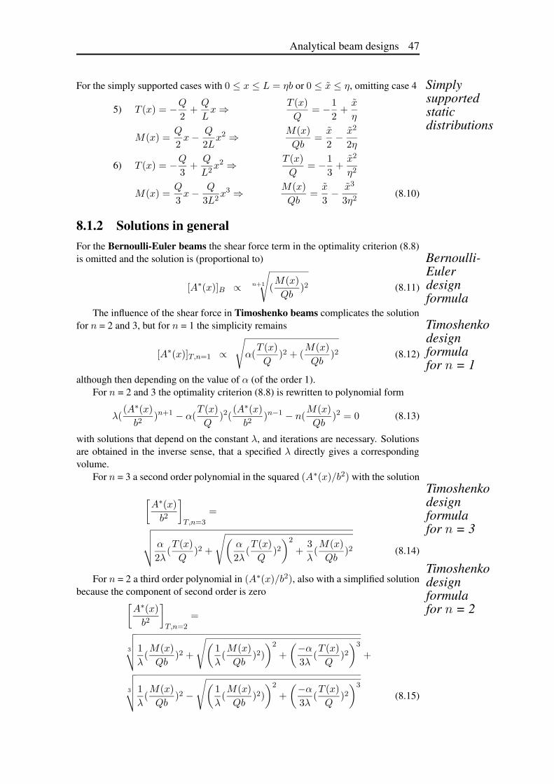
Analytical beam designs 47
For the simply supported cases with 0 ≤ x ≤ L = ηb or 0 ≤ x ≤ η, omitting case 4 Simplysupportedstaticdistributions
5) T (x) = −Q
2+
Q
Lx ⇒ T (x)
Q= −1
2+
x
η
M(x) =Q
2x − Q
2Lx2 ⇒ M(x)
Qb=
x
2− x2
2η
6) T (x) = −Q
3+
Q
L2x2 ⇒ T (x)
Q= −1
3+
x2
η2
M(x) =Q
3x − Q
3L2x3 ⇒ M(x)
Qb=
x
3− x3
3η2(8.10)
8.1.2 Solutions in generalFor the Bernoulli-Euler beams the shear force term in the optimality criterion (8.8)is omitted and the solution is (proportional to) Bernoulli-
Eulerdesignformula
[A∗(x)]B ∝ n+1
√
(M(x)
Qb)2 (8.11)
The influence of the shear force in Timoshenko beams complicates the solutionfor n = 2 and 3, but for n = 1 the simplicity remains Timoshenko
designformulafor n = 1
[A∗(x)]T,n=1 ∝√
α(T (x)
Q)2 + (
M(x)
Qb)2 (8.12)
although then depending on the value of α (of the order 1).For n = 2 and 3 the optimality criterion (8.8) is rewritten to polynomial form
λ((A∗(x)
b2)n+1 − α(
T (x)
Q)2(
(A∗(x)
b2)n−1 − n(
M(x)
Qb)2 = 0 (8.13)
with solutions that depend on the constant λ, and iterations are necessary. Solutionsare obtained in the inverse sense, that a specified λ directly gives a correspondingvolume.
For n = 3 a second order polynomial in the squared (A∗(x)/b2) with the solutionTimoshenkodesignformulafor n = 3
[
A∗(x)
b2
]
T,n=3
=
√
√
√
√
α
2λ(T (x)
Q)2 +
√
(
α
2λ(T (x)
Q)2)2
+3
λ(M(x)
Qb)2 (8.14)
Timoshenkodesignformulafor n = 2
For n = 2 a third order polynomial in (A∗(x)/b2), also with a simplified solutionbecause the component of second order is zero
[
A∗(x)
b2
]
T,n=2
=
3
√
√
√
√
1
λ(M(x)
Qb)2 +
√
(
1
λ(M(x)
Qb)2)
)2
+
(−α
3λ(T (x)
Q)2)3
+
3
√
√
√
√
1
λ(M(x)
Qb)2 −
√
(
1
λ(M(x)
Qb)2)
)2
+
(−α
3λ(T (x)
Q)2)3
(8.15)
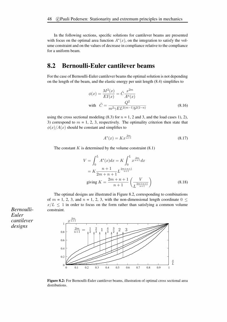
48 c©Pauli Pedersen: Stationarity and extremum principles in mechanics
In the following sections, specific solutions for cantilever beams are presentedwith focus on the optimal area function A∗(x), on the integration to satisfy the vol-ume constraint and on the values of decrease in compliance relative to the compliancefor a uniform beam.
8.2 Bernoulli-Euler cantilever beamsFor the case of Bernoulli-Euler cantilever beams the optimal solution is not dependingon the length of the beam, and the elastic energy per unit length (8.4) simplifies to
φ(x) =M2(x)
EI(x)= C
x2m
An(x)
with C =Q2
m2γEL2(m−1)b2(2−n)(8.16)
using the cross sectional modeling (8.3) for n = 1, 2 and 3, and the load cases 1), 2),3) correspond to m = 1, 2, 3, respectively. The optimality criterion then state thatφ(x)/A(x) should be constant and simplifies to
A∗(x) = Kx2mn+1 (8.17)
The constant K is determined by the volume constraint (8.1)
V =
∫ L
0A∗(x)dx = K
∫ L
0x
2mn+1 dx
= Kn + 1
2m + n + 1L
2m+n+1
n+1
giving K =2m + n + 1
n + 1
(
V
L2m+n+1
n+1
)
(8.18)
The optimal designs are illustrated in Figure 8.2, corresponding to combinationsof m = 1, 2, 3, and n = 1, 2, 3, with the non-dimensional length coordinate 0 ≤x/L ≤ 1 in order to focus on the form rather than satisfying a common volumeconstraint.Bernoulli-
Eulercantileverdesigns
0
0.2
0.4
0.6
0.8
1
0 0.1 0.2 0.3 0.4 0.5 0.6 0.7 0.8 0.9 1
PSfrag replacements
xL
x2mn+1
2mn+1
= 12
23
1 43
32
2 3
Figure 8.2: For Bernoulli-Euler cantilever beams, illustration of optimal cross sectional areadistributions.
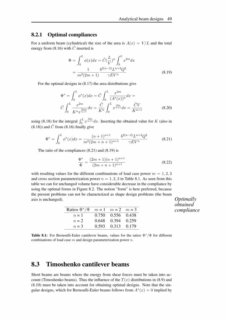
Analytical beam designs 49
8.2.1 Optimal compliancesFor a uniform beam (cylindrical) the size of the area is A(x) = V/L and the totalenergy from (8.16) with C inserted is
Φ =
∫ L
0φ(x)dx = C(
L
V)n
∫ L
0x2mdx
=1
m2(2m + 1)
b2(n−2)Ln+3Q2
γEV n(8.19)
For the optimal designs in (8.17) the area distributions give
Φ∗ =
∫ L
0φ∗(x)dx = C
∫ L
0
x2m
(A∗(x))ndx =
C
∫ L
0
x2m
Knx2mnn+1
dx =C
Kn
∫ L
0x
2mn+1 dx =
CV
Kn+1(8.20)
using (8.18) for the integral∫ L0 x
2mn+1 dx. Inserting the obtained value for K (also in
(8.18)) and C from (8.16) finally give
Φ∗ =
∫ L
0φ∗(x)dx =
(n + 1)n+1
m2(2m + n + 1)n+1
b2(n−2)Ln+3Q2
γEV n(8.21)
The ratio of the compliances (8.21) and (8.19) is
Φ∗
Φ=
(2m + 1)(n + 1)n+1
(2m + n + 1)n+1(8.22)
with resulting values for the different combinations of load case power m = 1, 2, 3and cross section parameterization power n = 1, 2, 3 in Table 8.1. As seen from thistable we can for unchanged volume have considerable decrease in the compliance byusing the optimal forms in Figure 8.2. The notion ”form” is here preferred, becausethe present problems can not be characterized as shape design problems (the beamaxis is unchanged). Optimally
obtainedcomplianceRatios Φ∗/Φ m = 1 m = 2 m = 3
n = 1 0.750 0.556 0.438n = 2 0.648 0.394 0.259n = 3 0.593 0.313 0.179
Table 8.1: For Bernoulli-Euler cantilever beams, values for the ratios Φ∗/Φ for differentcombinations of load case m and design parameterization power n.
8.3 Timoshenko cantilever beamsShort beams are beams where the energy from shear forces must be taken into ac-count (Timoshenko beams). Thus the influence of the T (x) distributions in (8.9) and(8.10) must be taken into account for obtaining optimal designs. Note that the sin-gular designs, which for Bernoulli-Euler beams follows from A∗(x) = 0 implied by
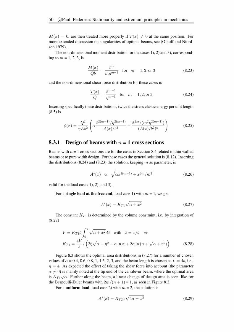
50 c©Pauli Pedersen: Stationarity and extremum principles in mechanics
M(x) = 0, are then treated more properly if T (x) 6= 0 at the same position. Formore extended discussion on singularities of optimal beams, see (Olhoff and Niord-son 1979).
The non-dimensional moment distribution for the cases 1), 2) and 3), correspond-ing to m = 1, 2, 3, is
M(x)
Qb=
xm
mηm−1for m = 1, 2, or 3 (8.23)
and the non-dimensional shear force distribution for these cases is
T (x)
Q=
xm−1
ηm−1for m = 1, 2, or 3 (8.24)
Inserting specifically these distributions, twice the stress elastic energy per unit length(8.5) is
φ(x) =Q2
γEb2
(
αx2(m−1)/η2(m−1)
A(x)/b2+
x2m/(m2η2(m−1))
(A(x)/b2)n
)
(8.25)
8.3.1 Design of beams with n = 1 cross sectionsBeams with n = 1 cross sections are for the cases in Section 8.4 related to thin walledbeams or to pure width design. For these cases the general solution is (8.12). Insertingthe distributions (8.24) and (8.23) the solution, keeping m as parameter, is
A∗(x) ∝√
αx2(m−1) + x2m/m2 (8.26)
valid for the load cases 1), 2), and 3).
For a single load at the free end, load case 1) with m = 1, we get
A∗(x) = KT1
√
α + x2 (8.27)
The constant KT1 is determined by the volume constraint, i.e. by integration of(8.27)
V = KT1b
∫ η
0
√
α + x2dx with x = x/b ⇒
KT1 =4V
b/(
2η√
α + η2 − α ln α + 2α ln (η +√
α + η2))
(8.28)
Figure 8.3 shows the optimal area distributions in (8.27) for a number of chosenvalues of α = 0.4, 0.6, 0.8, 1, 1.5, 2, 3, and the beam length is chosen as L = 4b, i.e.,η = 4. As expected the effect of taking the shear force into account (the parameterα 6= 0) is mainly noted at the tip end of the cantilever beam, where the optimal areais KT1
√α. Further along the beam, a linear change of design area is seen, like for
the Bernoulli-Euler beams with 2m/(n + 1) = 1, as seen in Figure 8.2.For a uniform load, load case 2) with m = 2, the solution is
A∗(x) = KT2x√
4α + x2 (8.29)
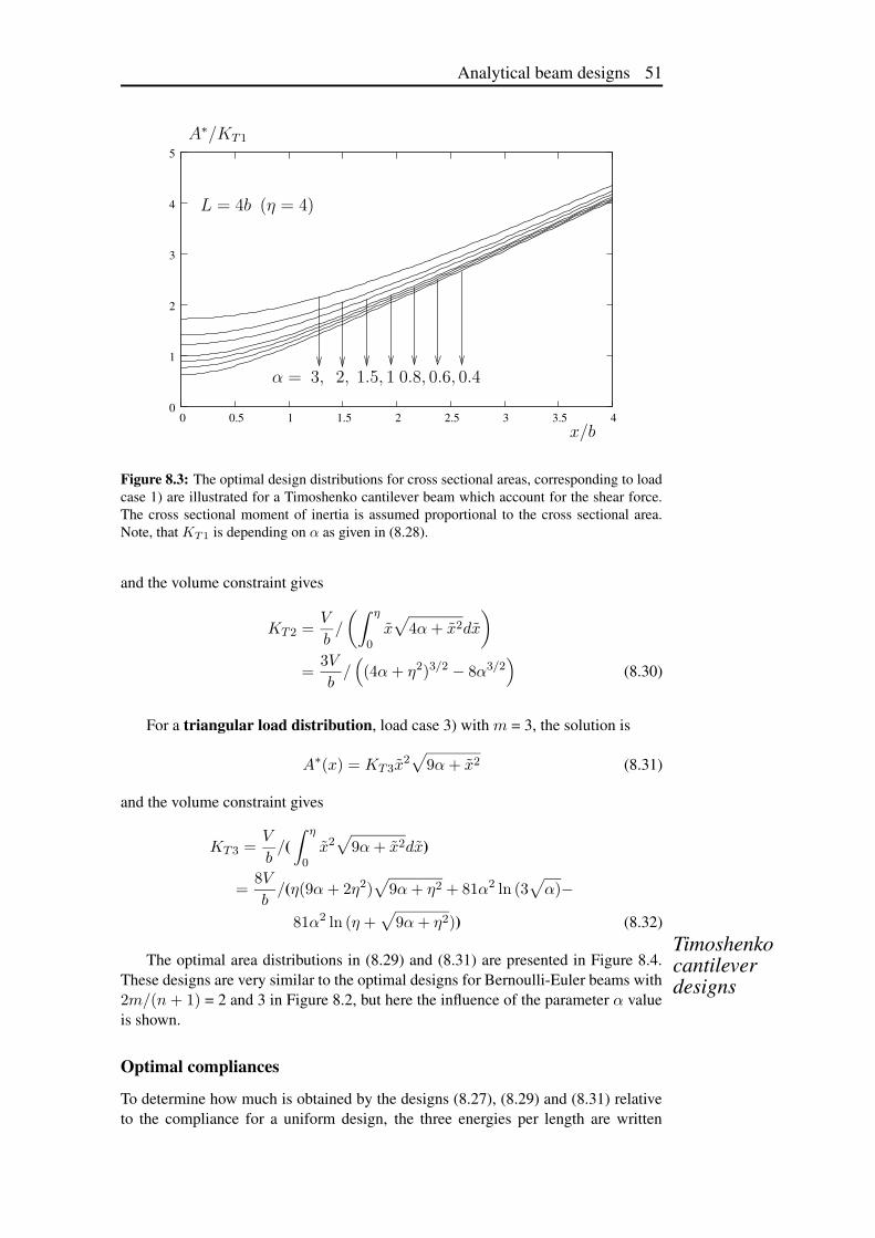
Analytical beam designs 51
0
1
2
3
4
5
0 0.5 1 1.5 2 2.5 3 3.5 4
PSfrag replacements
x/b
A∗/KT1
α = 3, 2, 1.5, 1 0.8, 0.6, 0.4
L = 4b (η = 4)
Figure 8.3: The optimal design distributions for cross sectional areas, corresponding to loadcase 1) are illustrated for a Timoshenko cantilever beam which account for the shear force.The cross sectional moment of inertia is assumed proportional to the cross sectional area.Note, that KT1 is depending on α as given in (8.28).
and the volume constraint gives
KT2 =V
b/
(∫ η
0x√
4α + x2dx
)
=3V
b/(
(4α + η2)3/2 − 8α3/2)
(8.30)
For a triangular load distribution, load case 3) with m = 3, the solution is
A∗(x) = KT3x2√
9α + x2 (8.31)
and the volume constraint gives
KT3 =V
b/(∫ η
0x2√
9α + x2dx)
=8V
b/(η(9α + 2η2)
√
9α + η2 + 81α2 ln (3√
α)−
81α2 ln (η +√
9α + η2)) (8.32)Timoshenkocantileverdesigns
The optimal area distributions in (8.29) and (8.31) are presented in Figure 8.4.These designs are very similar to the optimal designs for Bernoulli-Euler beams with2m/(n + 1) = 2 and 3 in Figure 8.2, but here the influence of the parameter α valueis shown.
Optimal compliancesTo determine how much is obtained by the designs (8.27), (8.29) and (8.31) relativeto the compliance for a uniform design, the three energies per length are written
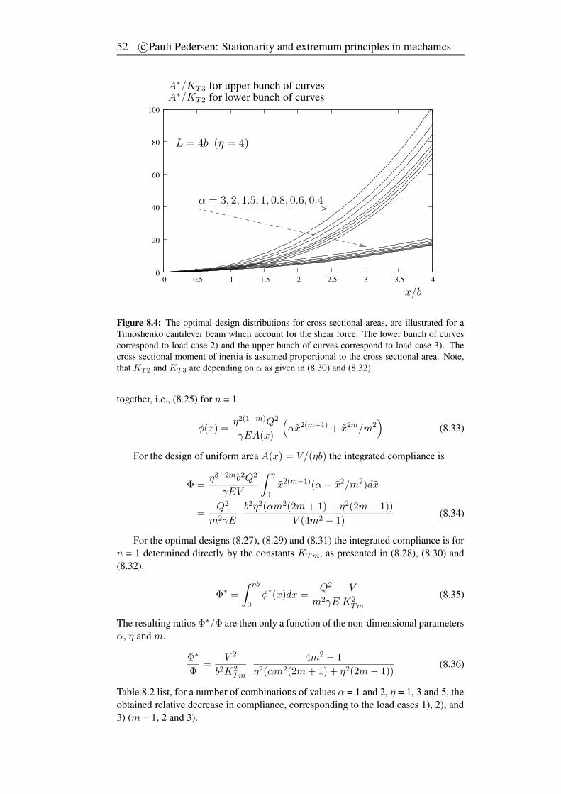
52 c©Pauli Pedersen: Stationarity and extremum principles in mechanics
0
20
40
60
80
100
0 0.5 1 1.5 2 2.5 3 3.5 4
PSfrag replacements
x/b
A∗/KT3 for upper bunch of curvesA∗/KT2 for lower bunch of curves
α = 3, 2, 1.5, 1, 0.8, 0.6, 0.4
L = 4b (η = 4)
Figure 8.4: The optimal design distributions for cross sectional areas, are illustrated for aTimoshenko cantilever beam which account for the shear force. The lower bunch of curvescorrespond to load case 2) and the upper bunch of curves correspond to load case 3). Thecross sectional moment of inertia is assumed proportional to the cross sectional area. Note,that KT2 and KT3 are depending on α as given in (8.30) and (8.32).
together, i.e., (8.25) for n = 1
φ(x) =η2(1−m)Q2
γEA(x)
(
αx2(m−1) + x2m/m2)
(8.33)
For the design of uniform area A(x) = V/(ηb) the integrated compliance is
Φ =η3−2mb2Q2
γEV
∫ η
0x2(m−1)(α + x2/m2)dx
=Q2
m2γE
b2η2(αm2(2m + 1) + η2(2m − 1))
V (4m2 − 1)(8.34)
For the optimal designs (8.27), (8.29) and (8.31) the integrated compliance is forn = 1 determined directly by the constants KTm, as presented in (8.28), (8.30) and(8.32).
Φ∗ =
∫ ηb
0φ∗(x)dx =
Q2
m2γE
V
K2Tm
(8.35)
The resulting ratios Φ∗/Φ are then only a function of the non-dimensional parametersα, η and m.
Φ∗
Φ=
V 2
b2K2Tm
4m2 − 1
η2(αm2(2m + 1) + η2(2m − 1))(8.36)
Table 8.2 list, for a number of combinations of values α = 1 and 2, η = 1, 3 and 5, theobtained relative decrease in compliance, corresponding to the load cases 1), 2), and3) (m = 1, 2 and 3).
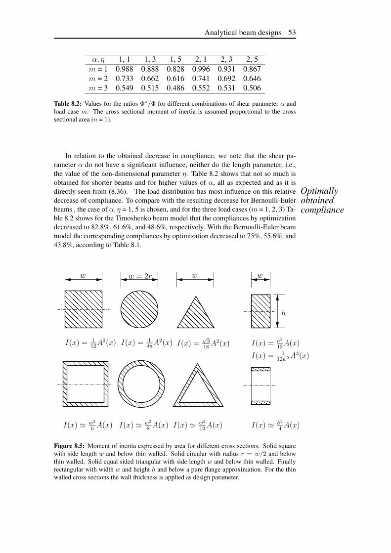
Analytical beam designs 53
α, η 1, 1 1, 3 1, 5 2, 1 2, 3 2, 5m = 1 0.988 0.888 0.828 0.996 0.931 0.867m = 2 0.733 0.662 0.616 0.741 0.692 0.646m = 3 0.549 0.515 0.486 0.552 0.531 0.506
Table 8.2: Values for the ratios Φ∗/Φ for different combinations of shear parameter α andload case m. The cross sectional moment of inertia is assumed proportional to the crosssectional area (n = 1).
In relation to the obtained decrease in compliance, we note that the shear pa-rameter α do not have a significant influence, neither do the length parameter, i.e.,the value of the non-dimensional parameter η. Table 8.2 shows that not so much isobtained for shorter beams and for higher values of α, all as expected and as it isdirectly seen from (8.36). The load distribution has most influence on this relative Optimally
obtainedcompliance
decrease of compliance. To compare with the resulting decrease for Bernoulli-Eulerbeams , the case of α, η = 1, 5 is chosen, and for the three load cases (m = 1, 2, 3) Ta-ble 8.2 shows for the Timoshenko beam model that the compliances by optimizationdecreased to 82.8%, 61.6%, and 48.6%, respectively. With the Bernoulli-Euler beammodel the corresponding compliances by optimization decreased to 75%, 55.6%, and43.8%, according to Table 8.1.
� � � � �� � � � �� � � � �� � � � �� � � � �
� � � � �� � � � �� � � � �� � � � �� � � � �
� � � � �� � � � �� � � � �� � � � �� � � � �
� � � � �� � � � �� � � � �� � � � �� � � � �
� � � � � � �� � � � � � �� � � � � � �� � � � � � �� � � � � � �
� � � � � � �� � � � � � �� � � � � � �� � � � � � �� � � � � � �
� �� �� �� �
� �� �� �� �
� �� �� �� �
� �
� �
� � � �� � � �� � � �� � � �
� � � �� � � �� � � �� � � �
� � � � �� � � � �� � � � �� � � � �
� � � � �� � � � �� � � � �� � � � �
� � � �� � � �� � � �� � � �� � � �
� � � �� � � �� � � �� � � �� � � �
PSfrag replacements
I(x) = 112
A2(x) I(x) = 14π
A2(x) I(x) =√
318
A2(x) I(x) = h2
12A(x)
I(x) = 112w2 A
3(x)
I(x) ' w2
6A(x) I(x) ' w2
8A(x) I(x) ' w2
12A(x) I(x) ' h2
4A(x)
www w = 2r
h
Figure 8.5: Moment of inertia expressed by area for different cross sections. Solid squarewith side length w and below thin walled. Solid circular with radius r = w/2 and belowthin walled. Solid equal sided triangular with side length w and below thin walled. Finallyrectangular with width w and height h and below a pure flange approximation. For the thinwalled cross sections the wall thickness is applied as design parameter.
54 c©Pauli Pedersen: Stationarity and extremum principles in mechanics
8.4 Examples of beam cross sectionsFigure 8.5 gives for a number of beam cross sections, the moment of inertia expressedin terms of the cross sectional area.
For thin walled beams the assumed uniform thickness t is also assumed relativelysmall and thus approximated directly by the areas. For the square 4wt(x) = A(x),for the circular πwt(x) = A(x), for the triangular 3wt(x) = A(x) and for the ”flangeor sandwich” beam 2wt(x) = A(x).
For the circular and the equal sided triangular cross sections I(x) is relative toany direction through the center of gravity. For the rectangular cross sections I(x) isrelative to the symmetry lines (also through the center of gravity).
8.5 Summing up• A large number of analytically (mostly explicit) optimal area distributions are
derived for compliance minimization with a given structural volume. This ispossible only for statically determinate cases, where the shear force distribu-tion T (x) and the moment distribution M(x) are independent of design. Thegraphical displays of these designs give the background for basic understand-ing of the influence from boundary conditions, from load distribution, andfrom the cross sectional modeling. Dealing with both long beams (Bernoulli-Euler model) and with short beams (Timoshenko beam model), the influencefrom shear force is made clear. All these different models are designed basedon an energy approach to directly obtain optimality criteria analytically.
• The direct energy approach has enabled a unified analysis for the specificcases, i.e., for three problems of cantilever beams and three problems of sim-ple supported beams, each with three cross sectional types, i.e., 18 cases forBernoulli-Euler beams and 18 cases for Timoshenko beams.
• The effect of optimization relative to uniform cross sectional design (cylindri-cal beam) also depends on these aspects, with optimal compliance values oftenhalf the original or even less, but also almost unchanged for specific cases.
• Taking the area distribution as design variable, then a numerical two or threedimensional model of a beam like structure may be compared. The obtainedoptimal volume distribution may be compared with A∗(x)dx from the presentstudy or A∗(x) may be used in an initial design for a similar or more compli-cated problem. Many cases are studied and the main parameters are related tothe integer values m = 1, 2, 3 and n = 1, 2, 3. The load distribution determinesm and the chosen cross sectional type is modeled with the power n.
• For long (Bernoulli-Euler) cantilever beams the optimal designs (8.17) aregiven by the function n+1
√x2m with Figure 8.2 showing these different forms.
Values for the obtained ratio of decreased compliance, relative to a uniformbeam (cylindrical beam), are listed in Table 8.1.
• For long (Bernoulli-Euler) simply supported beams the optimal beam designsalso depend on the length, expressed by the ratio of length over the chosencross sectional length parameter η = L/b. For these results see (Pedersenand Pedersen 2008), that also show results for Timoshenko simply supportedbeams.
Analytical beam designs 55
• For short (Timoshenko) cantilever beams the optimal designs, furthermore,are depending on the parameter α that describes the relative influence fromthe shear force. This parameter α = 2γβ(1 + ν) is depending on Poisson’sratio ν for the assumed isotropic material, on the shear stress distribution by β,and on a factor from cross sectional type γ. A practical range of 0.5 < α < 2is included in the chapter. For the ”thin walled” modeling (or pure width de-sign) of n = 1 the optimal design functions (8.27), (8.29) and (8.31) are stillsimple. Figure 8.3 shows optimal area functions for a load concentrated at thefree end and Figure 8.4 shows results for distributed loads. Details on con-straint scaling are presented and the obtained ratio of decreased compliancesfor chosen values of α, η and m are listed in Table 8.2.
• The cross sectional modeling cases of n = 2 and 3 give rise to a change fromdirect scaling in order to satisfy the volume constraint for the two solutions(8.14) and (8.15) that depend implicitly on the non-dimensional Lagrangianmultiplier λ. This constant is determined by simple bisection.

56 c©Pauli Pedersen: Stationarity and extremum principles in mechanics
Chapter 9
The ultimate optimal material
9.1 The individual constitutive parametersIn ultimate optimal material design, also named free material design, we representthe material properties in the most general form possible for an elastic continuum, Free
materialnamely the unrestricted set of components in positive semi-definite constitutive ma-trices.
For a given material (given constitutive relations), we normally measure cost bythe amount of material, say by thickness or density. With the free material we needa measure of the ”amount of a matrix”, and cost is then measured on the basis ofinvariants of these matrices.
With reference to the paper by (Bendsøe et al. 1994), we extend the results ob-tained in that paper to be valid also for power law non-linear elasticity, as done in(Pedersen 1998b). If we choose as cost constraint the Frobenius norm (length of amatrix) of the constitutive matrix, then the analytical proof of the optimal constitutive Frobenius
normmatrix, even for 3D-problems, is rather direct.
9.2 Sensitivity analysisWith localized sensitivity analysis as shown in chapter 4, and also given specificallyby (4.10), we have
duε
dh= −1
p
(
∂uε
∂h
)
fixed strains= −Ve
1
p
(
∂uε
∂he
)
fixed strains(9.1)
where Ve is the volume of the domain of the localized design variable he, (here a Localizeddeterminedsensitivities
component of the constitutive matrix). Thus minimum total strain energy uε impliesmaximum strain energy density uε in a fixed strain field. (In domains of non-constantstrain energy density, the notion of mean value uε should be used). The strain en-ergy density depends homogeneously on the squared effective strain εe, see (5.15) inchapter 5. The problem formulation can therefore be stated as Design
problemMaximize ε2e := {ε}T [α]{ε} subject to Frobenius([α]) = F([α]) = 1 (9.2)
where the matrix [α] describes the non-dimensional part of the constitutive matrix inthe secant formulation (??).
In the invariant formulation for [α] we can choose the coordinate system of prin-cipal strains
{ε}T = {{ε1 ε2 ε3} {0 0 0}} (9.3)
57
58 c©Pauli Pedersen: Stationarity and extremum principles in mechanics
and obtainPrincipalstrains only
ε2e = {ε}T [α]{ε} = {ε1 ε2 ε3}
α1111 α1122 α1133
α1122 α2222 α2233
α1133 α2233 α3333
ε1ε2ε3
(9.4)
Now, the Frobenius norm of a matrix is defined as the square root of the sumof the squares of all the elements of the matrix (equal to the squared length of thecontracted vector). It thus follows directly that for optimality, the matrix elementsnot involved in (9.4) must be zero. This means directly that also for the non-linear,Direct
conclusions power law materials we have:• the optimal material is orthotropic
• principal directions of material, strain and stress are aligned
• there is no shear stiffnessThis result for linear elastic material is proved in (Bendsøe et al. 1994), based
also on a constraint on the trace of the constitutive matrix. Here, the extension tonon-linear elastic material follows directly from the localized sensitivity result (9.1).For simplicity of proof we have chosen the Frobenius norm as the constraint.
9.3 Final optimizationThe further analysis relates only to the sub-matrix in (9.4). To fulfill the condition ofbeing positive definite, we have as necessary conditionsPositive
definite α1111 > 0, α2222 > 0, α3333 > 0
α1111α2222 > α21122, α1111α3333 > α2
1133, α2222α3333 > α22233 (9.5)
The problem formulation (9.1) can now be written as
Maximize ε2e = α1111ε
21 + α2222ε
22 + α3333ε
23 +
2α1122ε1ε2 + 2α1133ε1ε3 + 2α2233ε2ε3 (9.6)
constrained by (9.5) and by given Frobenius norm FNew designproblem F2 − 1 = α2
1111 + α22222 + α2
3333 + 2α21122 + 2α2
1133 + 2α22233 − 1 = 0 (9.7)
The general necessary condition for optimality is proportional gradients (seeOptimalitycondition (7.4) in chapter 7), i.e. for this specific case
d(ε2e)/dαiijj = λd(F2)/dαiijj (9.8)
with the same λ for all αiijj . This gives the result
ε21α1111
=ε22
α2222=
ε23α3333
=ε1ε2α1122
=ε1ε3α1133
=ε2ε3α2233
(9.9)
and we can finally write the resulting constitutive matrix in the directions of principalstrains/stresses (evaluating λ to satisfy (9.7):Optimal
modulusmatrix
[α]optimal =1
(ε1 + ε2 + ε3)2
ε21 ε1ε2 ε1ε3 0 0 0ε1ε2 ε22 ε2ε3 0 0 0ε1ε3 ε2ε3 ε23 0 0 00 0 0 0 0 00 0 0 0 0 00 0 0 0 0 0
(9.10)
Ultimate optimal material 59
9.4 Numerical aspects and comparisonwith isotropic material
The result (9.10) is valid also for power law, non-linear elastic materials. We note thatthe matrix in (9.10) has only one non-zero eigenvalue and that the material thereforeonly has stiffness in relation to the specified strain condition. For the ultimate optimalmaterial, the effective strain εe, the strain energy density uε, and the Frobenius normF are
ε2e = ε21 + ε2
2 + ε23
uε = E1
p + 1(ε21 + ε2
2 + ε23)
(p+1)/2
F = 1 (9.11)
We can obtain the same effective strain and strain energy density with an isotropic,zero Poisson’s ratio material [α] = [I], but then the corresponding Frobenius norm isF = 6, i.e. the material cost is six times greater. As shown in (Bendsøe et al. 1994),the zero Poisson’s ratio material may be valuable in numerical calculation, becauseof the degeneracy of the ultimate optimal material.
9.5 Summing upIn this chapter the important results to focus on are: Collected
results• The ultimate optimal material is very degenerate and is only stable in relation
to the specific strain state for which it is designed.
• The obtained solution is also valid for power law non-linear elastic materials,and simple arguments lead to the obtained analytical solution.
• The direct comparison with isotropic, zero Poisson’s ratio material is mostinteresting, and can be used for obtaining numerical solutions to specific prob-lems.

60 c©Pauli Pedersen: Stationarity and extremum principles in mechanics
References
Bendsøe, M. P., Guedes, J. M., Haber, R. B., Pedersen, P. and Taylor, J. E. (1994), ‘An ana-lytical model to predict optimal material properties in the context of optimal structuraldesign’, J. Applied Mechanics 61, 930–937.
Dems, K. and Mroz, Z. (1978), ‘Multiparameter structural shape optimization by finite ele-ment method’, Int. J. Numer. Meth. Engng. 13, 247–263.
Huang, N. C. (1968), ‘Optimal design of elastic structures for maximum stiffness’, Int. J.Solids Structures 4, 689–700.
Langhaar, H. L. (1962), Energy methods in applied mechanics, John Wiley and Sons, Inc.
Masur, E. F. (1970), ‘Optimum stiffness and strength of elastic structures’, J. Eng. Mech.Div., ASCE EM5, 621–649.
Olhoff, N. and Niordson, F. I. (1979), ‘Some problems concerning singularities of optimalbeams and columns’, Z A M M 59, T16–T26.
Olhoff, N. and Taylor, J. E. (1983), ‘On structural optimization’, Journal of Applied Mechan-ics 50, 1139–1151. 58 references.
Pedersen, N. L. (2004), ‘Optimization of holes in plates for control of eigenfrequencies’,Struct. Multidisc. Optim. 28(1), 1–10.
Pedersen, P. (1998a), Elasticity - Anisotropy - Laminates with Matrix Formulation, FiniteElement and Index to Matrices, Solid Mechanics, DTU, Kgs. Lyngby, Denmark. 320pages - also available at http://www.fam.web.mek.dtu.dk/html/pp.html.
Pedersen, P. (1998b), ‘Some general optimal design results using anisotropic power law non-linear elasticity’, Structural Optimization 15, 73–80.
Pedersen, P. (2003), ‘A note on design of fiber-nets for maximum stiffness’, J. of Elasticity73, 127–145.
Pedersen, P. (2005a), ‘Analytical stiffness matrices with Green-Lagrange strain measure’, Int.J. Numer. Meth. Engng. 62, 334–352.
Pedersen, P. (2005b), ‘Axisymmetric analytical stiffness matrices with Green-Lagrangestrains’, Computational Mechanics 35, 227–235.
Pedersen, P. (2006), ‘Analytical stiffness matrices for tetrahedral elements’, Computer Meth-ods in Applied Mechanics and Engineering 196, 261–278.
Pedersen, P. and Pedersen, N. L. (2008), ‘Analytical optimal designs for long and short stati-cally determinate beam structures’, Struct. Multidisc. Optim. pp. 1–15. on line.
Pedersen, P. and Taylor, J. E. (1993), Optimal design based on power-law non-linear elastic-ity, in P. Pedersen, ed., ‘Optimal Design with Advanced Materials,’, Elsevier, pp. 51–66.
Rozvany, G. N. I. (1989), Structural Design via Optimality Criteria, Kluwer, Dordrecht, TheNetherlands.
Save, M., Prager, W. and Sacchi, G. (1985), Structural optimization, optimality criteria,Vol. 1, Plenum Press.
61
62 c©Pauli Pedersen: Stationarity and extremum principles in mechanics
Sundstrøm, B., ed. (1998), Handbok och Formelsamling i Hallfasthetslaera (in Swedish),KTH, Stockholm. 398 pages.
Washizu, K. (1975), Variational methods in elasticity and plasticity, Pergamon Press, Ltd.
Wasiutynski, Z. (1960), ‘On the congruency of the forming according to the minimum po-tential energy with that according to equal strength’, Bull. de l’Academie Polonaise desSciences, Serie des Sciences Techniques 8(6), 259–268.
Index
admissibledisplacement field, 4stress field, 4
Also best strength, 35Analytical steps, 43Assumed power law elasticity, 17Assumptions, 11Available functions, 40
Basic assumption, 37beam cross sections
rectangular, 53solid circular, 53solid equal sided triangular, 53solid square, 53thin walled, 53
Beam length, 44Beam solutions by stress(complementary) principles, 30Bending energy only, 29Bending moment, 28Bernoulli-Euler cantilever beams, 48Bernoulli-Euler cantilever designs, 48Bernoulli-Euler design formula, 47
cantilever, slender beam, 30Castigliano’s 1st theorem, 7Castigliano’s 2nd theorem, 9Cauchy strains, 4Clapeyron’s theorem, 6Collected results, 41, 59complementary energy density, 26Complementary work of external loads, 5complementary(stress) virtual work, 8compliance decrease, 44Compliance from elastic energy, 5Compliance from potential of external loads, 5compliance minimization, 43Compliance objective, 44Compliance of external loads, 5Compliance per unit length, 45Conditions with a simple shape parametrization, 38Constant energy density, 36constitutive
individual parameter, 57matrix
non-dimensional, 57positive semi-definite matrix, 57
Constitutive secant modulus, 24Constitutive tangent modulus, 25Converted to non-constrained, 34corresponding displacement, 11cross sectional reference length, 45Cross sectional size, 44cross-sectional constants, 27cross-sectional forces/moments, 27curvature, 11
dead load, 6, 13
Decoupled energies, 28Derivatives of elastic potentials, 18Design for stiffness and strength, 38Design independent loads, 18, 36Design optimization, 33Design problem, 39, 57Detail of proof, 37differential strain energy density, 24Direct conclusions, 58direction
principal strain/stress, 58displacement control, 7displacement field, 4distribution of shear stresses, 45domain
non-shape, 37shape, 37
effectivestrain, 24, 57stress, 24
Effective strain/stress, 24Elastic energy in a straight beam, 27elastic strain energy, 17elastic stress energy, 17elasticity
power law non-linear, 36, 57Elementary case, 30Energy densities in 1D non-linear elasticity, 22Energy densities in 2D and 3D non-linear elasticity, 24Energy equilibrium, 17engineering strains, 4Equilibrium, 17equilibrium simplified, 17Estimated multiplier, 41Examples of beam cross sections, 54explicit analytical solution, 43External potential, 17External potential and compliance, 6extrema relations, 18extremum principle
for total complementary(stress)potential energy, 14for total potential energy, 13
Final optimization, 58finite element, 40fixed stress field, 37For model by the FEM, 40force equilibrium, 4Four energy solutions, 30Free material, 57Frobenius norm, 57
gamma-function, 39General knowledge, 35General optimization, 33General stress/strain state, 13
63
64 c©Pauli Pedersen: Stationarity and extremum principles in mechanics
geometrical constraint, 38given kinematic conditions, 7Goal of the chapter, 3Good experience, 38gradient of the elastic energy, 44
Handbook formulas, 27heuristic approach
successive iteration, 40homogeneous
energy relation, 34mass relation, 34
Homogeneous mass(volume) dependence, 34
identity, 4Inequality for mixed product, 12influence of beam length, 44Internal potentials, 17invariant
matrix, 57matrix length, 57
kinematically admissible, 4
Lagrangefunction, 34multiplier, 34, 40
linear elastic material, 6linear elasticity and dead loads, 6Linear strain notation, 21linear strains, 4Local design parameter, 18Localized determined sensitivities, 57Localized energy change, 36Localized volume change, 35
material designfree material, 57ultimate design, 57
material parameters, 27matrix invariant, 57maximize
eigenfrequency, 43stiffness, 43
maximum strain energy density, 57minimize compliance, 44minimum
compliance, 37maximum strain energy density, 37total strain energy, 57
Minimum complementary (stress) potential, 14Minimum potential, 13mixed products, 12Model for moment of inertia, 45moment distribution, 45moment equilibrium, 4Motivation for extremum, 11multidimensional stress/strain state, 13
necessary condition, 45a single constraint, 34non-constrained, 33positive definite, 58proportional gradient, 58proportionality, 34
necessary optimality criterion, 43Neglected shear energy, 29New design problem, 58No physical interpretation, 3Non-constrained problems, 33norm
Frobenius, 58Normal force, 27Not well known but important, 17Numerical aspects and comparison with isotropic mate-
rial, 59
optimal design formulation, 44optimal designs, 48optimal material
aligned, 58degenerate, 59no shear stiffness, 58non-zero eigenvalue, 59orthotropic, 58
Optimal modulus matrix, 58Optimality condition, 40, 58optimality condition, 34Optimality criterion, 45optimality criterion, 46Optimality criterion for beam design, 44Optimally obtained compliance, 49, 53optimize
material orientation, 33stiffness, 33strength, 33
outward normal, 3Overview of principles and their relations, 14
parametrizationboundary shape, 38super-ellipse, 38
Poisson’s ratio, 45zero, 59
Positive definite, 58Potential relations, 18Power law elasticity, 22Principal strains only, 58principle
of minimum total potential energy, 11overview, 14
Principle of minimum total complementary(stress) po-tential energy, 14
Principle of minimum total potential energy, 11principle of virtual displacements, 7principle of virtual stresses, 8Problems with a single constraint, 34Proportional gradients, 34Proportional relation, 24psi-function, 40
ratio of the compliances, 49real
displacement field, 6load field, 6strain field, 6stress field, 6
Real fields, 4Real stress field and real displacement field, 6Real stress field and virtual displacement field, 7Relations with power law elasticity, 18relative decrease in compliance, 52Relative hole area or density, 39Remark, 18Results for simple (Bernoulli-Euler) beams, 29
Secant and tangent modulus, 23secant formulation, 57Sensitivity analysis, 57sensitivity analysis
localized, 57shape optimization
References 65
stiffness, 36Shape optimization for stiffness and strength, 35shear force distribution, 45shear modulus, 45shear stresses, 28Simply supported static distributions, 47Single force behaviour, 11single load at the free end, 50singularities of optimal beams, 50six-dimensional strain/stress spaces, 13Size and shape, 33size optimization
stiffness, 34strength, 35
Size optimization for stiffness and strength, 34specialized principles, 7statically admissible, 4Statically determinate beams, 43statically determinate cases, 45Stationary objective, 33stationary total complementary potential, 19stationary total potential, 18Stationary total potential energy, 8Stationary total stress potential energy, 9Stiffest design, 35stiffest design
shape, 36size, 35
straineffective, 57principal, 57
Strain and stress energy densities, 21strain by differentiation, 21Strain energy density, 5, 21strain field, 4strength
von Mises, 35Strength or stiffness, 40stress by differentiation, 21stress energy
complementary formulation, 37Stress energy density, 5, 21stress field, 4Stress virtual work principle, 8strongest design
shape, 38size, 35
successive iterationheuristic approach, 40
Summing upchapter 8, 54chapter 6, 31chapter 5, 26chapter 3, 16chapter 7, 41chapter 4, 19chapter 2, 9chapter 9, 59
super-elliptic shape, 38surface area, 7surface traction’s, 4, 17Symbols and definitions, 4
tangent modulus, 23Tensor notation, 3The identity, 4The individual constitutive parameters, 57The work equation, 4The work equation, an identity, 3theorem
stiffest shape design, 37
strongest shape design, 38theorem of divergence, 3Timoshenko beam theory, 43Timoshenko cantilever beams, 49Timoshenko cantilever designs, 51Timoshenko design formula for n = 1, 47Timoshenko design formula for n = 2, 47Torsional moment, 28total external force, 45Total potential complementary energy, 5Total potential energy, 5Total potentials, 18Total strain energy, 5Total stress energy, 5Transverse force, 28triangular load distribution, 51Two or only one parameter, 38Two-sided bounds, 14
Uniaxial constitutive model, 13uniform load, 50uniform strain energy density, 35unit displacement field, 8Unit displacement theorem for linear elasticity, 8Unit load theorem for linear elasticity, 9Use of optimal design results, 44Using the theorem of divergence, 3
variational strain, 21variational strain energy density, 21variational stress energy density, 21Virtual fields, 4Virtual stress field and real displacement field, 8Virtual work principle, 7volume forces, 4
work equation, 4Work function, 12Work of external loads, 5
Young’s modulus, 45
Zero sum of total potentials, 6
Related Documents

![Extremum Seeking Control: Convergence Analysis · extremum seeking as one of the most promising adaptive control methods [1, Section 13.3]. There are two main approaches to extremum](https://static.cupdf.com/doc/110x72/5e1ecc5cc0fc09187723051d/extremum-seeking-control-convergence-analysis-extremum-seeking-as-one-of-the-most.jpg)