Testing the factor structure underlying behavior using ...

Testing the factor structure underlying behavior using joint cognitivemodels: Impulsivity in delay discounting and Cambridge gambling tasks

Peter D. KvamUniversity of Florida

Ricardo J. RomeuIndiana University

Brandon M. TurnerThe Ohio State University

Jasmin VassilevaVirginia Commonwealth University

Jerome R. BusemeyerIndiana University

Neurocognitive tasks are frequently used to assess disordered decision making, and cognitivemodels of these tasks can quantify performance in terms related to decision makers’ underlyingcognitive processes. In many cases, multiple cognitive models purport to describe similar pro-cesses, but it is difficult to evaluate whether they measure the same latent traits or processes.In this paper, we develop methods for modeling behavior across multiple tasks by connect-ing cognitive model parameters to common latent constructs. This approach can be used toassess whether two tasks measure the same dimensions of cognition, or actually improve theestimates of cognitive models when there are overlapping cognitive processes between tworelated tasks. The approach is then applied to connecting decision data on two behavioral tasksthat evaluate clinically-relevant deficits, the delay discounting task and Cambridge gamblingtask, to determine whether they both measure the same dimension of impulsivity. We find thatthe discounting rate parameters in the models of each task are not closely related, althoughsubstance users exhibit more impulsive behavior on both tasks. Instead, temporal discountingon the delay discounting task as quantified by the model is more closely related to externalizingpsychopathology like aggression, while temporal discounting on the Cambridge gambling taskis related more to response inhibition failures. The methods we develop thus provide a newway to connect behavior across tasks and grant new insights onto the different dimensions ofimpulsivity and their relation to substance use.

Keywords: intertemporal choice; joint cognitive model; neurocognitive task; substancedependence; Cambridge gambling task; measurement

This research was supported by the National Institute on DrugAbuse (NIDA) & Fogarty International Center under award num-ber R01DA021421, a NIDA Training Grant T32DA024628, andAir Force Office of Scientific Research / AFRL grants FA8650-16-1-6770 and FA9550-15-1-0343. Some of the content of this arti-cle was previously presented at the annual meetings of the Societyfor Mathematical Psychology (2019) and the Psychonomic Society(2018). The authors would like to thank all volunteers for their par-ticipation in this study. We express our gratitude to Georgi Vasilev,Kiril Bozgunov, Elena Psederska, Dimitar Nedelchev, Rada Nasled-nikova, Ivaylo Raynov, Emiliya Peneva and Victoria Dobrojalievafor assistance with recruitment and testing of study participants.Please address correspondence to Peter Kvam, 945 Center Dr., P.O.Box 112250, Gainesville, FL 32611, [email protected]

Introduction

Behavioral tasks are frequently used as a method of as-sessing patterns of performance that are indicative of dif-ferent kinds of cognitive deficits. For example, people withdeficits in working memory might perform worse on a taskthat requires them to recall information, or people with im-pulsive tendencies may find it difficult to wait for rewardsthat are delayed in time. By analyzing patterns of behavior,we can characterize the dysfunctions in decision-making thatpredict or result from different mental health or substanceuse disorders (Bickel & Marsch, 2001; Lejuez et al., 2003;MacKillop et al., 2011; Zois et al., 2014). In turn, we canunderstand how different traits put individuals at risk for sub-stance use or mental health problems, or design interventionsaimed at improving cognitive function to prevent or allevi-ate these problems (Bickel et al., 2016). Behavioral taskscan therefore grant insight onto traits or characteristics that

2 PETER D. KVAM

underlie risky, impulsive, or otherwise disordered decisionmaking both in the laboratory and the real world.

A critical assumption of this approach to assessing deci-sion behavior is that the behavioral tasks used in these ap-proaches provide measures of common underlying traits orcharacteristics that are related to disordered decision behav-ior. Naturally, each task is vetted for reliability and somedegree of predictive validity before putting into widespreaduse as assessment tools. Thus, there is typically good ev-idence to suggest that tasks like delay discounting are reli-able, reinforcing the view that they are measuring some sta-ble aspect of choice behavior (Simpson & Vuchinich, 2000).However, there are also multiple tasks that purport to mea-sure the same trait or characteristic using different experi-mental paradigms. This may be erroneous, as impulsivity isthought to be a multi-dimensional construct with as many asthree main factors: impulsive choice, impulsive action, andimpulsive personality traits (MacKillop et al., 2016). Impul-sive choice is thought to reflect the propensity to make de-cisions favoring an immediate reward over a larger delayedreward, impulsive action is thought to reflect the (in)abilityto inhibit motor responses, and impulsive personality is re-flected in self-report measures of individuals’ (in)ability toregulate their own actions.

Within each of these delineations, there are multiple tasksor methods that might serve as valid measures of one or moredimensions of impulsivity. For example, there are a numberof self-report and behavioral measures that are designed tomeasure people’s predispositions toward impulsive decision-making. Understanding the structure of impulsivity and howthese different measures are related is key for addressing anumber of health outcomes, as impulsivity is strongly im-plicated in a number of psychiatric disorders, most promi-nently ‘reinforcer pathologies’ (Bickel et al., 2011) such assubstance use disorders (Moeller et al., 2001; Dawe & Lox-ton, 2004) as well as eating disorders, gambling disorder, andsome personality disorders (Petry, 2001; De Wit, 2009). De-lay discounting in particular has been proposed as a primetransdiagnostic endophenotype of substance use disordersand other reinforcer pathologies (Bickel et al., 2014, 2012).Obtaining reliable estimates of impulsivity from behavioraltasks has both diagnostic and prognostic value, as it can notonly help identify at risk individuals, but also predict re-sponse to treatment, and offer the opportunity for effectiveearly prevention and interventions for addiction (Bickel et al.,2011; Conrod et al., 2010; Donohew et al., 2000; Vassileva& Conrod, 2018).

Because of the importance of impulsivity as a determi-nant of health outcomes, there have been a variety of dif-ferent paradigms designed to assess different dimensions ofimpulsive behavior. For example, both the Cambridge gam-bling task (Rogers et al., 1999) and delayed reward discount-ing task (Kirby et al., 1999) both aim to measure impul-

sive behavior, but they use largely different methods to doso. The Cambridge gambling task [CGT] measures impul-sivity by gauging decision-makers’ willingness to wait in or-der to make larger or smaller bets, generally requiring deci-sion makers to wait 5-20 seconds for potential bet values to“tick” up or down until it reaches the bet value they want towager. The decision maker experiences these delays in realtime during the experiment, waiting on each trial in orderto enter the bet they want to make as it comes on-screen.Conversely, delay discounting tasks [DDT] such as the Mon-etary Choice Questionnaire measure impulsivity as a func-tion of binary choices between two alternatives, where onealternative offers a smaller reward sooner / immediately andthe other alternative offers a larger reward at a later pointin time (Ainslie, 1974, 1975; Kirby et al., 1999). The taskparadigm for the CGT lends itself to understanding howpeople respond to short-term, experienced delays, while theDDT paradigm lends itself better to understanding how theyrespond to more long-term, described delays. While bothsituations can be construed as ones where people have toinhibit their impulses to take more immediate payoffs ver-sus greater delayed ones, which falls most naturally underimpulsive choice, it is possible that different dimensions ofimpulsivity are related to behavior on either task.

Computational models of such complex neurocognitivetasks parse performance into underlying neurocognitive la-tent processes and use the parameters associated with theseprocesses to understand the mechanisms of the specific neu-rocognitive deficits displayed by different clinical popula-tions (Ahn, Dai, et al., 2016). Research indicates that com-putational model parameters are more sensitive to dissociat-ing substance-specific and disorder-specific neurocognitiveprofiles than standard neurobehavioral performance indices(Haines et al., 2018; Vassileva et al., 2013; Ahn, Ramesh, etal., 2016). Similarly, dynamic changes in specific compu-tational parameters of decision-making, such as ambiguitytolerance, have been shown to predict imminent relapse inabstinent opioid-dependent individuals (Konova et al., 2019).This suggests that computational model parameters can serveas novel prognostic and diagnostic state-dependent markersof addiction that could be used for treatment planning.

Based on evidence from other task domains, it seemslikely that differences in behavioral paradigms may be sub-stantial enough to evaluate two dimensions or domains of im-pulsivity. In risky choice, clear delineations have been madebetween experience-based choice, where risks are learnedover time as a person experiences different reward frequen-cies, and description-based choice, where risks are describedin terms of percentages or proportions of the time they willsee rewards. The diverging behavior observed in these twoparadigms, referred to as the description-experience gap, il-lustrates that behavior under the two conditions need not lineup (Hau et al., 2008; Hertwig & Erev, 2009; Wulff et al.,

JOINT CLINICAL MODELING 3

2018). This appears to result from asymmetries in learn-ing on experience-based tasks, where people tend to learnmore quickly when they have under- versus over-predicteda reward (Haines et al., submitted). Given the evidence forthis type of gap in risky choice, it seems likely that a similardifference between described (DDT) and experienced (CGT)delays may result in diverging behavior due to participantslearning from their experiences of the delays.1 Of course, itis not necessarily the case that such a gap exists for the CGTand DDT paradigms and how they measure impulsivity, butthe diverging patterns of behavior in risky choice should atleast raise suspicion about the effects of described versus ex-perienced delays in temporal discounting.

Approach

So how do we test if these two different tasks are measur-ing the same underlying dimension of impulsivity as mea-sures of impulsive choice? The remaining part of the pa-per is devoted to answering this question. The first step isto gather data on both tasks from the same participants, sothat we can measure whether individual differences in impul-sive choice are expressed in observed behavior on both tasks.For this, we utilize data from a large study on impulsivity inlifetime substance dependent (in protracted abstinence) andhealthy control participants in Bulgaria (Ahn et al., 2014;Vassileva et al., 2018; Ahn & Vassileva, 2016). This sam-ple includes both “pure” (mono-substance dependent) heroinand amphetamine users as well polysubstance dependent in-dividuals and healthy controls. The majority of substancedependent participants in these studies were in protracted ab-stinence (i.e., not active users, and were screened prior toparticipation to ensure they had no substances in their sys-tem) but met the lifetime DSM-IV criteria for heroin, am-phetamine, or polysubstance dependence. They were alsonot on methadone maintenance or on any other medication-assisted therapy, unlike most abstinent opiate users in theUnited States. This participant sample has multiple benefitsfor the current effort: it both provides a set of participantswho are likely to be highly impulsive, increasing the varianceon trait impulsivity; and it provides an opportunity to com-pare the performance of the models we examine in terms oftheir ability to predict substance use outcomes.

The second step in testing whether the two tasks reflectthe same dimension of impulsive choice is to quantify be-havior on the tasks in terms of the component cognitive pro-cesses. This is done by using cognitive models to describeeach participant’s behavior in terms of contributors like at-tention, memory, reward sensitivity, and those relevant to im-pulsivity such as temporal discounting (Busemeyer & Stout,2002). Each parameter in the model corresponds to a particu-lar piece of the cognitive processes underlying task behavior,and improves predictions of related self-report and outcomemeasures over basic behavioral metrics like choice propor-

tions or mean response times (Fridberg et al., 2010; Romeuet al., 2019). They therefore serve as the most complete anduseful descriptors of behavior on cognitive tasks, and theirparameters correspond theoretically to individual differencesin cognition.

The third step is to construct a model of both tasks byrelating parameters of the cognitive models of each task tocommon underlying factors like impulsivity. This is far fromstraightforward, as it requires both theoretical and method-ological innovations. In terms of theory, a modeler has tomake determinations about which parameters should be re-lated to common latent constructs, and therefore how modelparameters should relate to one another across tasks. Forour present purposes this is made reasonably straightforward,as the most common models of both Cambridge gamblingand delay discounting tasks include parameters describingtemporal discounting rates that determine how the subjectivevalue of a prospect decreases with delays, but in other casesit may be a case of exploratory factor analysis (using cog-nitive latent variable model structures like we describe be-low) and/or model comparison between different latent fac-tor structures. From a practical standpoint, the modeler alsorequires methods for simultaneously fitting the parametersof both models along with the latent factor values. Usinga hierarchical Bayesian approach, Turner et al. (2013) de-veloped a joint modeling approach to simultaneously predictneural and behavioral data from participants performing asingle task. These methods connect two sources of data toa common underlying set of parameters, either constraininga single cognitive model using multiple sources of informa-tion (Turner et al., 2016) or connecting separate models vialatent factor structures (Turner et al., 2017). The benefit ofthe joint modeling approach is that all sources of data are for-mally incorporated into the model by specifying an overarch-ing, typically hierarchical structure. As shown in a variety ofapplications (Turner et al., 2013, 2015, 2016, 2017), model-ing the co-variation of each data modality can provide strongconstraints on generative models, and these constraints canlead to better predictions about withheld data when the cor-relation between at least one latent factor is nonzero (Turner,2015).

Similarly, Vandekerckhove (2014) developed methods forconnecting personality inventories to cognitive model param-eters, creating a cognitive latent variable model structure thatpredicts both self-report and response time (and accuracy)data from the same participants simultaneously. As with thejoint modeling approach, it allows data from one measure

1Notwithstanding post-experiment consequences of the choices,such as playing out a randomly selected question. While these con-sequences help to make the selections more real, a participant doesnot receive experiential feedback about their choice before makinganother selection, and thus this experience is irrelevant to observedbehavior on the task.

4 PETER D. KVAM

to inform another by linking them to a common underlyingfactor. In this paper, we develop methods based on the jointmodeling and cognitive latent variable modeling approachesthat can be used to connect behavior on multiple cognitivetasks to a common set of latent factors.

Finally, we must test the factor structure underlying taskperformance by comparing different models against one an-other. Depending on how the models are fit, different met-rics will be available for model comparison. Taking advan-tage of the fully Bayesian approach, we provide a methodfor arbitrating between different model factor structures us-ing a Savage-Dickey approximation of the Bayes factor (Wa-genmakers et al., 2010). This method is particularly usefulbecause it allows us to find support for the hypothesis thatthe relationship between parameters is zero, indicating thatperformance on the different tasks is not related to a com-mon underlying factor but to separate ones. In effect, weuse the Bayes factor to compare a 1-factor against a 2-factormodel, directly yielding a metric describing the support forone model over the other given the data available.

To preview the results, the Bayes factor for all groups(amphetamine, heroin, polysubstance, and controls) favorsa multi-dimensional model of impulsivity in delay discount-ing and Cambridge gambling tasks, suggesting that the dif-ferent paradigms measure impulsive action and impulsivechoice / personality. This is an interesting result in itself,but also serves to illustrate how the joint modeling and cog-nitive latent variable modeling approaches can be used tomake novel inferences about the factor structure underlyingdifferent tasks. The remainder of the paper is devoted to themethods for developing and testing these models, with modelcode provided to assist others in carrying out these types ofinvestigations.

Background methods

Although both tasks are relatively well-established astools in clinical assessment, it is helpful to examine how eachone assesses impulsivity, both in terms of raw behavior and interms of model parameters. We first cover the basic structureof the delay discounting and Cambridge gambling task, thenthe most common models of each task, and finally how theycan be put together using a joint modeling framework.

It is worth noting that there are several competing modelsof the delay discounting task. For our purposes, we primarilyexamine the hyperbolic discounting model (Chung & Herrn-stein, 1967; Kirby & Herrnstein, 1995; Mazur, 1987), as itis presently the most widely used model of preference fordelayed rewards. However, we repeat many of the analysespresented in this paper by using an alternate attention-basedmodel of delay discounting, the direct difference model (Dai& Busemeyer, 2014), in Appendix A. The main conclusionsof the paper do not change depending on which model isused, but the direct difference model tends to fit better for

some substance use groups and its parameters are somewhatmore closely related to the Cambridge gambling task modelparameters.

Tasks

A total of 399 participants took part in a study on im-pulsivity among substance users in Sofia, Bulgaria. This in-cluded 75 “pure” heroin users, 73 “pure” amphetamine uses,98 polysubstance users, and 153 demographically matchedcontrols, including siblings of heroin and amphetamineusers. Lifetime substance dependence was assessed usingDSM-IV criteria, and all participants were in protracted ab-stinence (met the DSM-IV criteria for sustained full remis-sion).

In addition to the Monetary Choice Questionnaire of de-lay discounting and the Cambridge gambling task describedbelow, all participants also completed 11 psychiatric mea-sures including an IQ assessment using Raven progressivematrices (Raven, 2000), the Fagerström test for nicotine de-pendence (Heatherton et al., 1991), structured interviews andthe screening version of the Psychopathy Checklist (Hart etal., 1995; Hare, 2003), and the Wender Utah rating scale forADHD (Ward, 1993). They also completed personality mea-sures including the Barratt Impulsiveness Scale (Patton etal., 1995), the UPPS Impulsive Behavior Scale (Whiteside& Lynam, 2001), the Buss-Warren Aggression Question-naires (Buss & Warren, 2000), the Levenson self-report psy-chopathy scale (Levenson et al., 1995), and the Sensation-Seeking Scale (Zuckerman et al., 1964). The other behav-ioral measures they completed included the Iowa GamblingTask (Bechara et al., 1994), the Immediate Memory Task(Dougherty et al., 2002), the Balloon Analogue Risk Task(Lejuez et al., 2002, 2003), the Go/No-go task (Lane et al.,2007), and the Stop Signal task (Dougherty et al., 2005).These are used later on to assess which dimensions of im-pulsivity are predicted by which model parameters.

Below we describe the main tasks of interest: the MCQdelay discounting task and the Cambridge gambling task.The participants in these tasks were recruited as part of alarger study on impulsivity, and they completed both tasks,allowing us to assess the relation between performance onthe DDT and the CGT for each person and for each group towhich they belonged. More details on the study and partic-ipant recruitment are provided in Ahn et al. (2014) and Ahn& Vassileva (2016).

Delay discounting task. The delay discounting taskwas developed for use in behavioral studies of animal popu-lations as a measure of impulse control (Chung & Herrnstein,1967; Ainslie, 1974). Performance on the delay discountingtask has been linked to a number of important health out-comes, including substance dependence (Bickel & Marsch,2001) and a propensity for taking safety risks (Daugherty &Brase, 2010). Task performance and the parameters of the

JOINT CLINICAL MODELING 5

cognitive model (the hyperbolic discounting model) are fre-quently used as an indicator of temporal discounting, impul-sivity, and a lack of self-control (Ainslie & Haslam, 1992).

The structure of each trial of the delay discounting taskfeatures a choice between two options. The first is a smallerreward (e.g., $10 immediately), so-called the “smaller,sooner” (SS) option. The second is a larger reward (e.g.,$15) at a longer delay (e.g., 2 weeks), referred to as the“larger, later” (LL) option. This study used the Mone-tary Choice Questionnaire designed by Kirby & Marakovic(1996), which features 27 choices between SS and LL op-tions. Often, impulsivity is quantified as simply the propor-tion of responses in favor of the SS option, reflecting an over-all tendency to select options with shorter delays. However,this can be confounded with choice variability – participantswho choose more randomly regress toward 50% SS and LLselections, which may make them appear more or less impul-sive relative to other participants in a data set. Therefore, themodel we use includes a separate choice variability param-eter, which describes how consistently a person chooses anoption that they would appear to subjective value higher. Theremaining temporal discounting parameter k then quantifieshow much options are valued dependent on their delay.

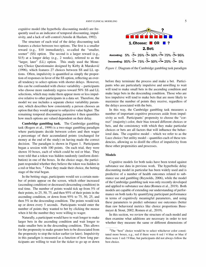
Cambridge gambling task. The Cambridge gamblingtask (Rogers et al., 1999) is a two-stage gambling paradigmwhere participants decide between colors and then wagera percentage of their accumulated points (exchanged formoney at the end of the study) on having made the correctdecision. The paradigm is shown in Figure 1. Participantsbegan a session with 100 points. On each trial, they wereshown 10 boxes, each of which could be red or blue. Theywere told that a token was hidden randomly (uniform distri-bution) in one of the boxes. In the choice stage, the partici-pant responded whether they believe the token was hidden ina red or blue box. 2 Once they made their choice, the bettingstage of the trial began.

In the betting stage, participants would see a certain num-ber of points appear on the screen, which either increased(ascending condition) or decreased (descending condition) inreal time. The number of points would tick up from 5% oftheir points, to 25, 50, 75, and then 95% of their points in theascending condition, or down from 95% to 75, 50, 25, andthen 5% in the descending condition. The points would tickup or down every 5 seconds. Participants would enter thenumber of points they wanted to bet by clicking the mousewhen it hit the number they were willing to wager.

Naturally, a participant would have to wait longer to makelarger bets in the ascending condition and wait longer tomake smaller bets in the descending condition. This allowsfor the propensity to make greater bets to be dissociated fromthe propensity to stop the ticker earlier (or later). Impulsivityin this paradigm is measured as a function of how long par-ticipants are willing to wait for the ticker to go up or down

Figure 1. Diagram of the Cambridge gambling task paradigm

before they terminate the process and make a bet. Partici-pants who are particularly impulsive and unwilling to waitwill tend to make small bets in the ascending condition andmake large bets in the descending condition. Those who areless impulsive will tend to make bets that are more likely tomaximize the number of points they receive, regardless ofthe delays associated with the bets.

In this way, the Cambridge gambling task measures anumber of important cognitive processes aside from impul-sivity as well. Participants’ propensity to choose the “cor-rect” (majority) color, their bias toward different choices orbets, and the consistency with which they make particularchoices or bets are all factors that will influence the behav-ioral data. The cognitive model – which we refer to as theLuce choice / bet utility model – quantifies each of these ten-dencies, allowing us to distill the effect of impulsivity fromthese other propensities and processes.

Models

Cognitive models for both tasks have been tested againstsubstance use data in previous work. The hyperbolic delaydiscounting model in particular has been widely used and ispredictive of a number of health outcomes related to sub-stance use and gambling (Reynolds, 2006), while the modelof the Cambridge gambling task was only recently developedand applied to substance use data (Romeu et al., 2019). Bothmodels are capable of extending our understanding of perfor-mance on both tasks by quantifying participant performancein terms of cognitively meaningful parameters, and usingthese parameters to predict substance use outcomes (betterthan raw behavioral metrics like choice proportions Buse-meyer & Stout, 2002; Romeu et al., 2019).

In this section, we review the structure of each model andthen examine what additions are necessary in order to testwhether they measure the same or different dimensions of

2The “best” choice would be to select whichever color consti-tuted more boxes, e.g., red if there were 6 red / 4 blue or blue ifthere were 1 red / 9 blue, but participants did not always follow thebest choice.

6 PETER D. KVAM

impulsivity. Both models contain a parameter related to tem-poral discounting, where outcomes that are delayed have asubjectively lower value. Higher values of these parameterslead participants to select options that are closer in time andare therefore linked to impulsivity, so it is only natural totry connecting them to a common latent factor. The jointmodeling method we present allows us to do so, as well aspermits us to test whether they are measuring the same un-derlying construct using a nested model comparison with aBayes factor.

In the following sections we focus on the hyperbolic dis-counting model of the delay discounting task, but a descrip-tion of the direct difference model – which fits several of thesubstance use groups better than the hyperbolic model – isalso presented in Appendix A.

Hyperbolic discounting model. Although early ac-counts of how rewards are discounted as they are displacedin time followed a constant discounting rate, represented inan exponential discounting function derived from behavioraleconomic theory (Camerer, 1999), the most common modelof discounting behavior instead uses a hyperbolic function(Ainslie & Haslam, 1992; Mazur, 1987), which generally fitshuman discounting behavior better and accounts for morequalitative patterns such as preference reversals (Kirby &Herrnstein, 1995; Kirby & Marakovic, 1995; Dai & Buse-meyer, 2014). Certainly, other models could be used to ac-count for behavior on this task, and we test one such model inthe Appendix (the direct difference model Dai & Busemeyer,2014; Cheng & González-Vallejo, 2016). Fortunately, the ex-act model of discounting behavior seems not to substantiallyaffect the conclusions of the procedure reported here.

The hyperbolic discounting model uses two parameters.The first is a discounting rate k, which describes the rate atwhich a payoff (x) decreases in subjective value (v(x, t)) as itis displaced in time (t).

v(x, t) =1

1+ k · t(1)

Higher values of k will result in options that are furtheraway in time being discounted more heavily. Since delaydiscounting generally features one smaller, sooner option andone larger, later option, a higher k will result in more choicesin favor of the smaller, sooner option because the greater im-pact of the delay in the later option.

The second parameter m determines how likely a personis to choose one option over another given their subjectivevalues v(x1, t1) and v(x2, t2). The probability of choosing thelarger, later option (x2, t2; where x2 > x1 and t2 > t1) is givenas

Pr(choose LL) =1

1+ exp(−m · [v(x2, t2)− v(x1, t1)])(2)

Higher values of m will make alternatives appear moredistinctive in terms of choice proportions, resulting in a moreconsistent choice probability. Lower values for m make al-ternatives appear more similar, driving choice probabilitiestoward 0.5.

Because the estimates of k tend to be heavily right-skewed, it is typical to estimate log(k) instead of k to have anindicator of impulsivity that is close to normally distributed.Therefore, we use the same natural log transformation of kwhen estimating its value in all of the models presented here– this is particularly important in the joint model, where theexponential of the underlying impulsivity trait value must betaken to obtain the k values for each individual (Figure 2).

Luce choice / bet utility model. The Luce choice / betutility model for the Cambridge gambling task uses four pa-rameters, reduced by one from the original model presentedby Romeu et al. (2019) in order to reduce the likelihood offailing to recover parameters due to correlations among them(in the original model, there was a utility parameter assignedto bet payoffs, but this frequently traded off with the bet vari-ability parameter γ, described below). The first two param-eters α and c affect the probability of choosing red or blueas the favored box color. The value of c controls the bias forchoosing red or blue. A value greater than .5 indicates a biastoward choosing red, whereas a value less than .5 indicates abias toward choosing blue. The value of α determines howresponsive a decision maker is to shifts in the number of redand blue boxes. Greater values of α will make a person moresensitive to the number of boxes and therefore more likely toselect whichever color appears in greater proportion, whereassmaller values of α will make them less sensitive to the pro-portion of red and blue boxes and therefore more likely toselect randomly. Put together, the probability of choosing‘red’ as the favored box color, Pr(R), is given as a functionof the number of red boxes (NR; a number between 0 and 10)and the parameters α and c:

Pr(R) =c ·Nα

Rc ·Nα

R +(1− c) · (10−NR)α(3)

The probability of giving different bet values (either 5%,25%, 50%, 75%, or 95%) depends on the decision made dur-ing the choice stage as well as on the parameters relevantto behavior on the betting component of the CGT. Once achoice is made, the bet is conditioned on that decision. Inparticular, the probability of the prior choice being correctenters into the probability of making different bets. Formally,the expected utility of making any particular bet (EU(B),where B is a proportion between 0 and 1) is computed asa function of the likelihood of being correct (Pr(C)) and thecurrent number of points (pts).3

3Note that this simply uses a linear utility rather than a powerfunction. This is mainly because including the additional parameterfor the exponent of a power utility function introduces strong inter-

JOINT CLINICAL MODELING 7

Figure 2. Diagram of the structure of the joint model.

EU(B) = pts · (Pr(C) · (1+B)+(1−Pr(C)) · (1−B)) (4)

If a decision maker selected their highest-utility optionswith no effect of delay, then they would simply stop thecounter when it reached the bet (out of B =.05, .25, .5, .75,or .95) that maximized EU(B) regardless of the time it tookthe ticker to reach that bet value. However, time becomes afactor when waiting imposes a cost that affects the utility ofthe different bets. This is accounted for by including an ad-ditional parameter β that describes the cost associated withwaiting one additional unit of time. The amount of time aperson has to wait to make a particular bet TB depends onwhether they are in the ascending or descending ticker con-dition, such that, for B =.05, .25, .5, .75, or .95, respectively:

TB =

{0,1,2,3,4 if ascending4,3,2,1,0 if descending

(5)

The adjusted utility of giving a particular bet AU(B,β) isthen given by multiplying the cost of each unit of time β bythe time associated with the bet TB:

,β) = EU(B)−β ·TB (6)

Finally, these adjusted utilities for the possible bets enterinto Luce’s choice rule (Luce, 1959) to map their continuousexpected utilities into a probability of making each possi-ble bet b = {b1,b2,b3,b4,b5} = {.05, .25, .5, .75, .95}. Theconsistency with which a decision maker selects the highest-utility bet is determined by the bet variability parameter γ.Higher values of γ correspond to more consistently choosing

the highest-utility bet, while lower values of γ lead a personto choose more randomly:

Pr(B = bi) =exp(γ ·AU(bi,β))

5∑j=1

exp(γ ·AU(b j,β))

(7)

Note that this is the same Luce choice rule used to deter-mine the probabilities of making different choices (Equation3). To obtain the joint distribution of choice and bet proba-bilities – i.e., the likelihood we actually want to estimate –this must be calculated for both “red” and “blue” choices. Intotal, this yields a probability distribution over the 10 possi-ble selections: Pr(C = red,B = .05), Pr(C = blue,B = .05),Pr(C = red,B = .25), and so on.

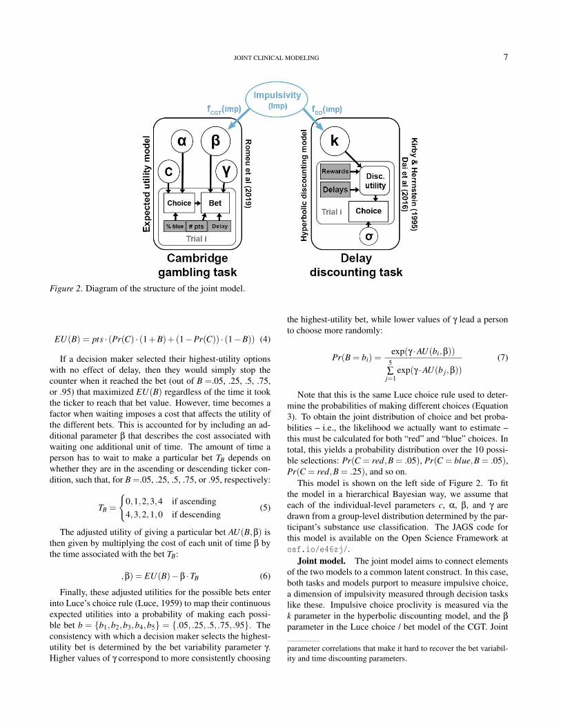
This model is shown on the left side of Figure 2. To fitthe model in a hierarchical Bayesian way, we assume thateach of the individual-level parameters c, α, β, and γ aredrawn from a group-level distribution determined by the par-ticipant’s substance use classification. The JAGS code forthis model is available on the Open Science Framework atosf.io/e46zj/.

Joint model. The joint model aims to connect elementsof the two models to a common latent construct. In this case,both tasks and models purport to measure impulsive choice,a dimension of impulsivity measured through decision taskslike these. Impulsive choice proclivity is measured via thek parameter in the hyperbolic discounting model, and the β

parameter in the Luce choice / bet model of the CGT. Joint

parameter correlations that make it hard to recover the bet variabil-ity and time discounting parameters.

8 PETER D. KVAM

models are theoretically capable of putting together manydifferent tasks and measures, but as this is the first time ithas been applied to modeling behavior across tasks, we havechosen to make the process simple by only connecting thetwo models. Therefore, the number of new elements neededto construct the joint model is minimal.

One of the innovations here is to add a latent variable ontop of the cognitive model parameters that describes a deci-sion maker’s underlying tendency toward impulsive choice.This is shown as the blue region of Figure 2. This Impulsivity(Imp) variable is then mapped onto k and β values throughlinking functions fDDT (Imp) and fCGT (Imp), respectively.In essence, we are constructing a structural equation modelwhere the measurement component of the model consists ofan established cognitive model of the task. The advantageof using cognitive models over a simple statistical mapping(usually linear with normal distributions in structural equa-tion modeling) is that the cognitive models are able to betterreflect not only performance on the task but the putative gen-erative cognitive processes. This makes the parameters of themodel, including the estimated values of impulsivity and theconnections between the tasks, more meaningful and morepredictive of other outcomes (Busemeyer & Stout, 2002).

To connect the Impulsivity variable to k in the hyperbolicdiscounting model, we used a simple exponential link func-tion

k = fDDT (Imp) = exp(Imp) (8)

Readers familiar with structural equation modeling willknow that one of the parameters of the model will need tobe fixed in order to identify them. This is done by fixing theloading of k onto Impulsivity to be 1; there is no free param-eter in fDDT . Conversely, the load of β onto Impulsivity addstwo free parameters as part of a linear mapping, including anintercept (giving a difference in mean between log(k) and β)and slope (mapping variance in log(k) or Imp to variance inβ).

β = fCGT (Imp) = b0 +bCGT · Imp (9)

The remaining parameters inherited from the constituentmodels are m (DDT) and α, γ, and c (CGT). This essentiallycompletes the joint model. The Impulsivity values for eachindividual are set hierarchically, so that each person has a dif-ferent value for Imp but they are constrained by a group-leveldistribution of impulsivity from their substance use group.The values of b0 and bCGT are not set hierarchically but ratherfixed within a group, as variation in these parameters acrossparticipants would not be distinguishable from variation inImp values.

Simulation studies

One of the most fundamentally important aspects of test-ing a cognitive model is to ensure that it can capture trueshifts in the parameters underlying behavior (Heathcote etal., 2015). This is difficult to assess using real data, as wedo not know the parametric structure of the true generatingprocess. Instead, a modeler can simulate a set of artificialdata from a model with a specific set of parameters and thenfit the model to that data in order to see if the estimates cor-respond to the true underlying parameters that were used tocreate the data in the first place. This model recovery pro-cess ensures that the parameter estimates in the model canbe meaningful; if model recovery fails and we are unable toestimate parameters of a true underlying cognitive process,then there is nothing we can conclude from the parameterestimates because they do not reflect the generating process.If model recovery is reasonably successful, then at least wecan say that it is possible to apply the model to estimate someproperties of the data.

This is particularly important to note because the hyper-bolic discounting model – a popular account of performanceon the delay discounting task – can often be hard to recoverusing classical methods like maximum likelihood estimationor even non-hierarchical Bayesian methods (Molloy et al, inprep). This problem can be addressed by using a hierarchicalBayesian approach where parameter estimates for individualparticipants are constrained by a group-level distribution andvice versa (Kruschke, 2014; Shiffrin et al., 2008). The five-parameter version of the Cambridge gambling task (Romeuet al, 2019) suffers from similar issues, but when reducedto four parameters by reducing the power function used forcomputing utilities to a linear utility and fit in a hierarchicalBayesian way, it is possible to recover as well.

For both models, the simulated data were generated so thatthey would mimic the properties of the real data to which themodel was later applied. To this end, the simulations used150 participants (approximately the size of a larger substanceuse group; similar but slightly less precise results can also beobtained for 50- or 100-participant simulations), 27 uniquedata points per participant for the delay discounting task,and 200 unique data points per participant for the Cambridgegambling task. Participants in the real CGT task varied interms of the number of points they had accumulated goinginto each trial, meaning that the bets they could place coulddiffer from trial to trial. To compensate for this, the simu-lated trials randomly selected from a range of possible pointvalues (from 5 [the minimum] to 200 points) as the startingvalue for each trial. The rest of the task variables – includ-ing payoffs and delays in the DDT, and box proportions andascending/descending manipulation in the CGT – were setaccording to their real values in the experiments.

The hyperbolic discounting model used the k, m parame-ter specification, where k is the discounting rate and m cor-

JOINT CLINICAL MODELING 9

-6 -4 -2 0 2

Actual value

-6

-4

-2

0

2

Estim

ate

d v

alu

eDiscounting rate (k)

r = 0.83

= 0.84

0 20 40

Actual value

0

10

20

30

40

50

Estim

ate

d v

alu

e

Choice variability (m)

r = 0.75

= 0.90

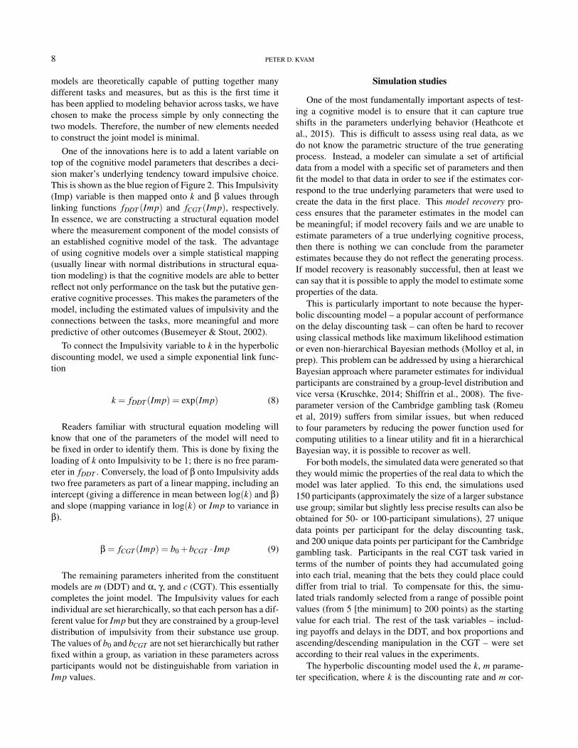
Figure 3. Parameter recovery for data simulated from thehyperbolic discounting model (DDT) parameters when thetask data are fit alone.

responds to the choice variability parameter in a softmax de-cision rule. Thanks to the hierarchical constraints imposedon the individual-level parameters, it was possible to recoverboth of these parameters with reasonable precision when thedelay discounting task was fit individually. The results of thesimulation and recovery are shown in Figure 3. The x-axisdisplays the true value of each individual’s k or m value, andthe y-axis displays the value estimated from the model. Thevalues of k are shown on a log scale, as these values tendto be much closer to log-normally than normally distributed.The linear (r) and rank (ρ) correlations are also displayed asheuristics for assessing how well these parameters were re-covered. While the quality was generally good, particularlyconsidering there were only 27 unique data points for eachparticipant, there is potential room for improvement in esti-mating each parameter. As we show later, the joint modelcan actually assist in improving the quality of fits like thesewhere data is sparse.

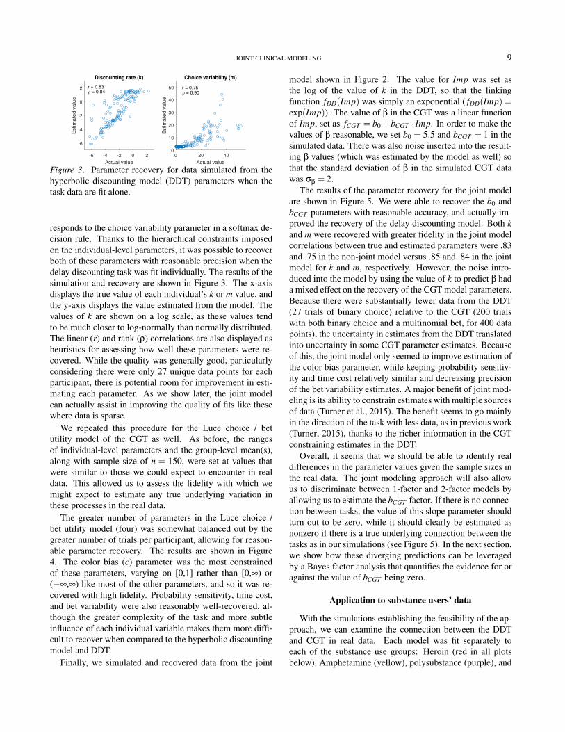
We repeated this procedure for the Luce choice / betutility model of the CGT as well. As before, the rangesof individual-level parameters and the group-level mean(s),along with sample size of n = 150, were set at values thatwere similar to those we could expect to encounter in realdata. This allowed us to assess the fidelity with which wemight expect to estimate any true underlying variation inthese processes in the real data.

The greater number of parameters in the Luce choice /bet utility model (four) was somewhat balanced out by thegreater number of trials per participant, allowing for reason-able parameter recovery. The results are shown in Figure4. The color bias (c) parameter was the most constrainedof these parameters, varying on [0,1] rather than [0,∞) or(−∞,∞) like most of the other parameters, and so it was re-covered with high fidelity. Probability sensitivity, time cost,and bet variability were also reasonably well-recovered, al-though the greater complexity of the task and more subtleinfluence of each individual variable makes them more diffi-cult to recover when compared to the hyperbolic discountingmodel and DDT.

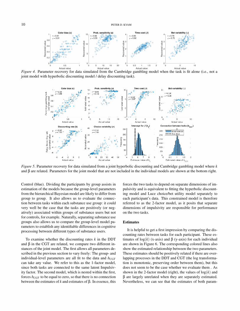
Finally, we simulated and recovered data from the joint

model shown in Figure 2. The value for Imp was set asthe log of the value of k in the DDT, so that the linkingfunction fDD(Imp) was simply an exponential ( fDD(Imp) =exp(Imp)). The value of β in the CGT was a linear functionof Imp, set as fCGT = b0 +bCGT · Imp. In order to make thevalues of β reasonable, we set b0 = 5.5 and bCGT = 1 in thesimulated data. There was also noise inserted into the result-ing β values (which was estimated by the model as well) sothat the standard deviation of β in the simulated CGT datawas σβ = 2.

The results of the parameter recovery for the joint modelare shown in Figure 5. We were able to recover the b0 andbCGT parameters with reasonable accuracy, and actually im-proved the recovery of the delay discounting model. Both kand m were recovered with greater fidelity in the joint modelcorrelations between true and estimated parameters were .83and .75 in the non-joint model versus .85 and .84 in the jointmodel for k and m, respectively. However, the noise intro-duced into the model by using the value of k to predict β hada mixed effect on the recovery of the CGT model parameters.Because there were substantially fewer data from the DDT(27 trials of binary choice) relative to the CGT (200 trialswith both binary choice and a multinomial bet, for 400 datapoints), the uncertainty in estimates from the DDT translatedinto uncertainty in some CGT parameter estimates. Becauseof this, the joint model only seemed to improve estimation ofthe color bias parameter, while keeping probability sensitiv-ity and time cost relatively similar and decreasing precisionof the bet variability estimates. A major benefit of joint mod-eling is its ability to constrain estimates with multiple sourcesof data (Turner et al., 2015). The benefit seems to go mainlyin the direction of the task with less data, as in previous work(Turner, 2015), thanks to the richer information in the CGTconstraining estimates in the DDT.

Overall, it seems that we should be able to identify realdifferences in the parameter values given the sample sizes inthe real data. The joint modeling approach will also allowus to discriminate between 1-factor and 2-factor models byallowing us to estimate the bCGT factor. If there is no connec-tion between tasks, the value of this slope parameter shouldturn out to be zero, while it should clearly be estimated asnonzero if there is a true underlying connection between thetasks as in our simulations (see Figure 5). In the next section,we show how these diverging predictions can be leveragedby a Bayes factor analysis that quantifies the evidence for oragainst the value of bCGT being zero.

Application to substance users’ data

With the simulations establishing the feasibility of the ap-proach, we can examine the connection between the DDTand CGT in real data. Each model was fit separately toeach of the substance use groups: Heroin (red in all plotsbelow), Amphetamine (yellow), polysubstance (purple), and

10 PETER D. KVAM

0 0.5 1

Actual value

0

0.2

0.4

0.6

0.8

1

Reco

vere

d v

alu

e

Color bias (c)

r = 0.91

= 0.91

0 5 10 15 20

Actual value

0

5

10

15

Reco

vere

d v

alu

e

Prob. sensitivity (a)

r = 0.66

= 0.55

0 0.5 1 1.5 2

Actual value

0

1

2

3

4

Reco

vere

d v

alu

e

Time cost ( )

r = 0.84

= 0.82

0 5 10

Actual value

0

1

2

3

4

Reco

vere

d v

alu

e

Bet variability ( )

r = 0.79

= 0.75

Figure 4. Parameter recovery for data simulated from the Cambridge gambling model when the task is fit alone (i.e., not ajoint model with hyperbolic discounting model / delay discounting task).

Figure 5. Parameter recovery for data simulated from a joint hyperbolic discounting and Cambridge gambling model where kand β are related. Parameters for the joint model that are not included in the individual models are shown at the bottom right.

Control (blue). Dividing the participants by group assists inestimation of the models because the group-level parametersfrom the hierarchical Bayesian model are likely to differ fromgroup to group. It also allows us to evaluate the connec-tion between tasks within each substance use group: it couldvery well be the case that the tasks are positively (or neg-atively) associated within groups of substance users but notfor controls, for example. Naturally, separating substance usegroups also allows us to compare the group-level model pa-rameters to establish any identifiable differences in cognitiveprocessing between different types of substance users.

To examine whether the discounting rates k in the DDTand β in the CGT are related, we compare two different in-stances of the joint model. The first allows all parameters de-scribed in the previous section to vary freely: The group- andindividual-level parameters are all fit to the data and bCGTcan take any value. We refer to this as the 1-factor model,since both tasks are connected to the same latent Impulsiv-ity factor. The second model, which is nested within the first,forces bCGT to be equal to zero, so that there is no connectionbetween the estimates of k and estimates of β. In essence, this

forces the two tasks to depend on separate dimensions of im-pulsivity and is equivalent to fitting the hyperbolic discount-ing model and Luce choice/bet utility model separately toeach participant’s data. This constrained model is thereforereferred to as the 2-factor model, as it posits that separatedimensions of impulsivity are responsible for performanceon the two tasks.

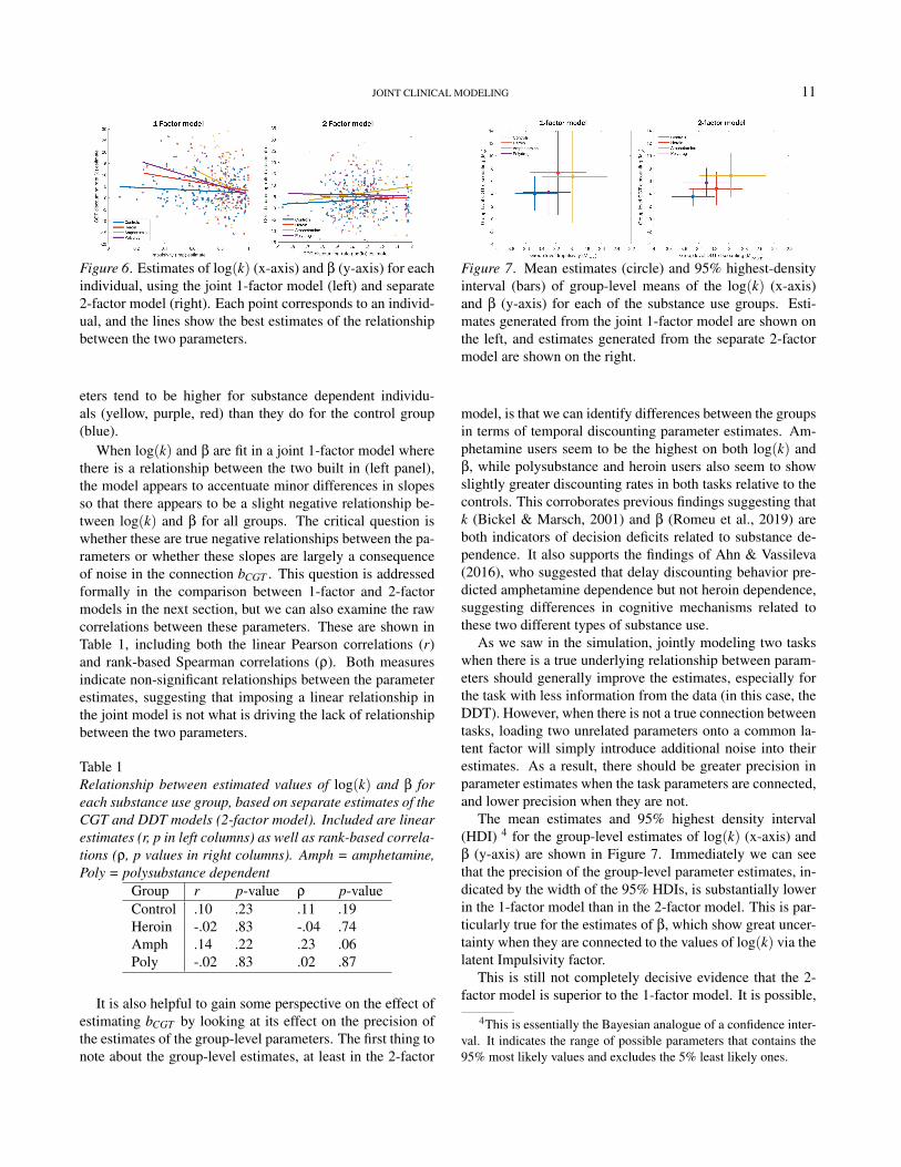
Estimates

It is helpful to get a first impression by comparing the dis-counting rates between tasks for each participant. These es-timates of log(k) (x-axis) and β (y-axis) for each individualare shown in Figure 6. The corresponding colored lines alsoshow the estimated relationship between the two parameters.These estimates should be positively related if there are over-lapping processes in the DDT and CGT (the log transforma-tion is monotonic, preserving order between them), but thisdoes not seem to be the case whether we evaluate them . Asshown in the 2-factor model (right), the values of log(k) andβ are largely unrelated when they are separately estimated.Nevertheless, we can see that the estimates of both param-

JOINT CLINICAL MODELING 11

Figure 6. Estimates of log(k) (x-axis) and β (y-axis) for eachindividual, using the joint 1-factor model (left) and separate2-factor model (right). Each point corresponds to an individ-ual, and the lines show the best estimates of the relationshipbetween the two parameters.

eters tend to be higher for substance dependent individu-als (yellow, purple, red) than they do for the control group(blue).

When log(k) and β are fit in a joint 1-factor model wherethere is a relationship between the two built in (left panel),the model appears to accentuate minor differences in slopesso that there appears to be a slight negative relationship be-tween log(k) and β for all groups. The critical question iswhether these are true negative relationships between the pa-rameters or whether these slopes are largely a consequenceof noise in the connection bCGT . This question is addressedformally in the comparison between 1-factor and 2-factormodels in the next section, but we can also examine the rawcorrelations between these parameters. These are shown inTable 1, including both the linear Pearson correlations (r)and rank-based Spearman correlations (ρ). Both measuresindicate non-significant relationships between the parameterestimates, suggesting that imposing a linear relationship inthe joint model is not what is driving the lack of relationshipbetween the two parameters.

Table 1Relationship between estimated values of log(k) and β foreach substance use group, based on separate estimates of theCGT and DDT models (2-factor model). Included are linearestimates (r, p in left columns) as well as rank-based correla-tions (ρ, p values in right columns). Amph = amphetamine,Poly = polysubstance dependent

Group r p-value ρ p-valueControl .10 .23 .11 .19Heroin -.02 .83 -.04 .74Amph .14 .22 .23 .06Poly -.02 .83 .02 .87

It is also helpful to gain some perspective on the effect ofestimating bCGT by looking at its effect on the precision ofthe estimates of the group-level parameters. The first thing tonote about the group-level estimates, at least in the 2-factor

Figure 7. Mean estimates (circle) and 95% highest-densityinterval (bars) of group-level means of the log(k) (x-axis)and β (y-axis) for each of the substance use groups. Esti-mates generated from the joint 1-factor model are shown onthe left, and estimates generated from the separate 2-factormodel are shown on the right.

model, is that we can identify differences between the groupsin terms of temporal discounting parameter estimates. Am-phetamine users seem to be the highest on both log(k) andβ, while polysubstance and heroin users also seem to showslightly greater discounting rates in both tasks relative to thecontrols. This corroborates previous findings suggesting thatk (Bickel & Marsch, 2001) and β (Romeu et al., 2019) areboth indicators of decision deficits related to substance de-pendence. It also supports the findings of Ahn & Vassileva(2016), who suggested that delay discounting behavior pre-dicted amphetamine dependence but not heroin dependence,suggesting differences in cognitive mechanisms related tothese two different types of substance use.

As we saw in the simulation, jointly modeling two taskswhen there is a true underlying relationship between param-eters should generally improve the estimates, especially forthe task with less information from the data (in this case, theDDT). However, when there is not a true connection betweentasks, loading two unrelated parameters onto a common la-tent factor will simply introduce additional noise into theirestimates. As a result, there should be greater precision inparameter estimates when the task parameters are connected,and lower precision when they are not.

The mean estimates and 95% highest density interval(HDI) 4 for the group-level estimates of log(k) (x-axis) andβ (y-axis) are shown in Figure 7. Immediately we can seethat the precision of the group-level parameter estimates, in-dicated by the width of the 95% HDIs, is substantially lowerin the 1-factor model than in the 2-factor model. This is par-ticularly true for the estimates of β, which show great uncer-tainty when they are connected to the values of log(k) via thelatent Impulsivity factor.

This is still not completely decisive evidence that the 2-factor model is superior to the 1-factor model. It is possible,

4This is essentially the Bayesian analogue of a confidence inter-val. It indicates the range of possible parameters that contains the95% most likely values and excludes the 5% least likely ones.

12 PETER D. KVAM

given enough noise in an underlying latent variable, that thejoint model could be reflecting true uncertainty about Impul-sivity and properly reflecting this uncertainty in correspond-ing estimates of β and log(k). The factor structure compar-ison presented next is aimed at formally addressing whichmodel is supported by the data.

Factor structure comparison

The 2-factor model is nested within the 1-factor model,where the differentiating factor is that the 2-factor model re-moves the connection between the two tasks. In some ways,the 2-factor model can be thought as a nested model wherebCGT = 0. As such, tests based on classical null hypothesissignificance testing cannot provide support for the 2-factormodel, because they could only reject or fail to reject (notsupport) the hypothesis that the slope of this relationship iszero. Instead, we use a method of approximating a Bayesfactor called the Savage-Dickey density ratio BF01, whichcan provide support for or against a model that claims a zerovalue for a parameter (Verdinelli & Wasserman, 1995; Wa-genmakers et al., 2010). It does so by comparing the densityof the prior distribution at zero against the posterior densityat zero. Formally, it computes the ratio

BF01 =Pr(H = 0|D)

Pr(H = 0)(10)

where H is the parameter / hypothesis under consideration,and D is the set of data being used to inform the model. Thevalue of Pr(H) is the prior, while Pr(H|D) is the posterior.

Data generated from a process with a true value of H , 0will decrease our belief that a parameter value is zero, result-ing in a posterior distribution where Pr(H = 0|D)< Pr(H =0) and therefore BF01 < 1. Conversely, a data set which in-creases our belief that a parameter value is zero will resultin a posterior distribution where Pr(H = 0|D) < Pr(H = 0)and thus BF01 > 1. In essence, the Bayes factor is quantifyinghow much our belief that the parameter value (hypothesis) iszero changes in light of the data.

Applied to the problem at hand, we are interested in howmuch our belief about bCGT being equal to zero changes inlight of the delay discounting and Cambridge gambling taskdata. An increase in the credibility of bCGT being zero isevidence for the 2-factor model, whereas a decrease in thecredibility of bCGT being zero is evidence for the 1-factormodel.

Naturally, the outcome of this test will depend on the priorprobability distribution we set for bCGT . In this application,we have tried to make the prior as reasonable as possibleby setting Pr(bCGT ) ∼ N(0,10). This allows a reasonableamount of flexibility for the parameter to take many values(improving the potential for model fit) while also providing asuitably high prior probability of Pr(bCGT = 0) (which willmove the Bayes factor toward favoring the 1-factor model).

Some readers may disagree over the value of the prior, whichwill affect the Bayes factor. The prior distribution is shownin Figure 8 for each comparison, which allows a reader tojudge for themselves what sorts of priors would still yieldthe same result. Almost any reasonable set of normally dis-tributed priors with standard deviation greater than 1 for thecontrol / polysubstance groups or greater than 4 for the am-phetamine / heroin groups will still yield evidence in favor ofbCGT = 0.

Figure 8. Diagram of the Savage-Dickey Bayes factor anal-ysis. The posterior likelihood of no relation between the twotasks (darker distributions) is compared to the prior likeli-hood of no relation between them (lighter distributions) todetermine whether the data increased or decreased supportfor a relationship between parameters of the different tasks.

As shown in Figure 8, the Bayes factors all favor the 2-factor model, with BF01 varying between 6 and 37. For refer-ence, a Bayes factor of 3-10 is typically thought to constitute“moderate” or “substantial” evidence, a Bayes factor of 10-30 constitutes “strong” evidence, and a Bayes factor of 30 ormore “very strong” evidence (Jeffreys, 1961; Lee & Wagen-makers, 2014). The evidence therefore favors the 2-factormodel across all of the substance use groups at a moderate tostrong level.

Of course, the Bayes factors and thus the interpretation ofthe strength of evidence may change according to the priors.However, the posteriors generally suggest that the evidencecan and should favor the 2-factor model. For the control andpolysubstance groups, the posterior distributions are centeredso close to zero that almost any choice of prior will still resultin a Bayes factor favoring the 2-factor model, and the heroinand amphetamine groups (notably, the groups with the small-est number of participants) provide evidence in opposing di-rections.

Overall, putting together the low correlation between pa-rameters when the models are estimated separately (2-factor;

JOINT CLINICAL MODELING 13

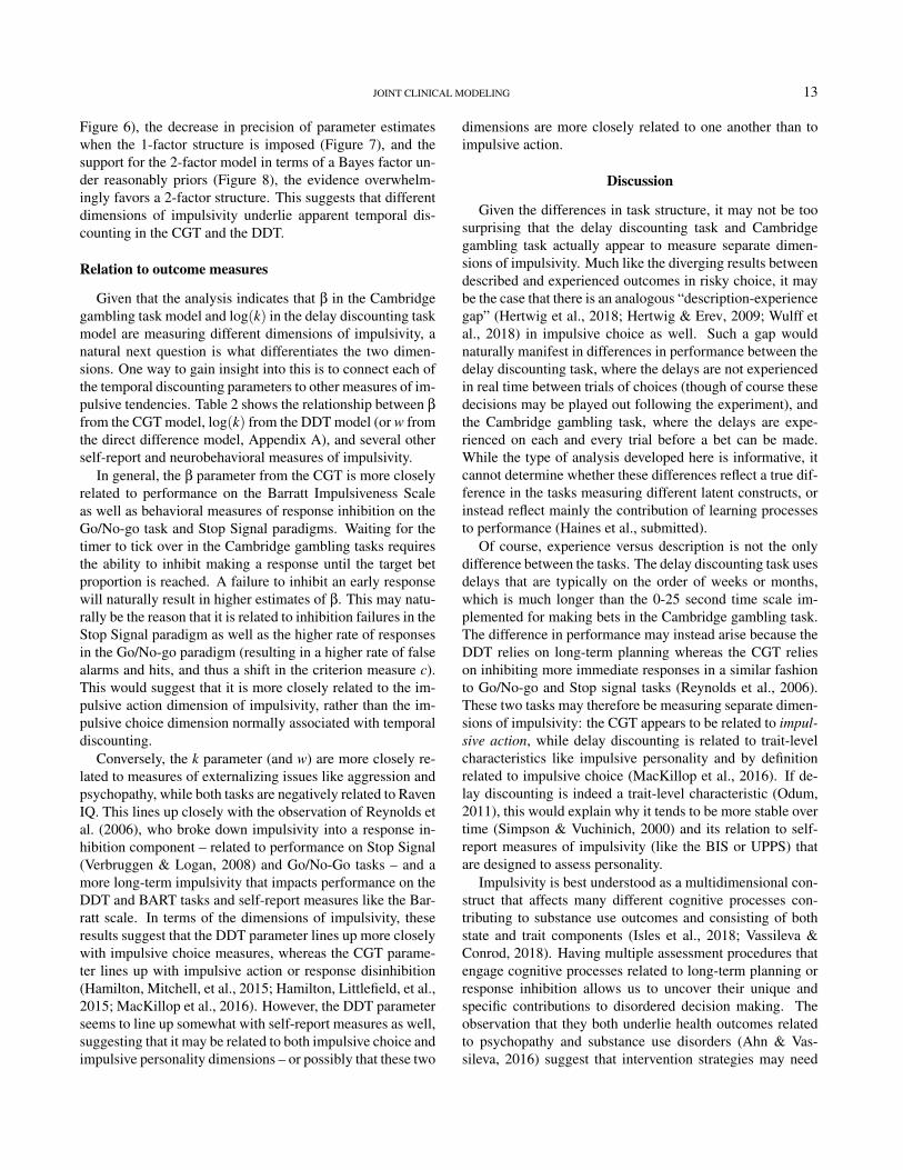
Figure 6), the decrease in precision of parameter estimateswhen the 1-factor structure is imposed (Figure 7), and thesupport for the 2-factor model in terms of a Bayes factor un-der reasonably priors (Figure 8), the evidence overwhelm-ingly favors a 2-factor structure. This suggests that differentdimensions of impulsivity underlie apparent temporal dis-counting in the CGT and the DDT.

Relation to outcome measures

Given that the analysis indicates that β in the Cambridgegambling task model and log(k) in the delay discounting taskmodel are measuring different dimensions of impulsivity, anatural next question is what differentiates the two dimen-sions. One way to gain insight into this is to connect each ofthe temporal discounting parameters to other measures of im-pulsive tendencies. Table 2 shows the relationship between β

from the CGT model, log(k) from the DDT model (or w fromthe direct difference model, Appendix A), and several otherself-report and neurobehavioral measures of impulsivity.

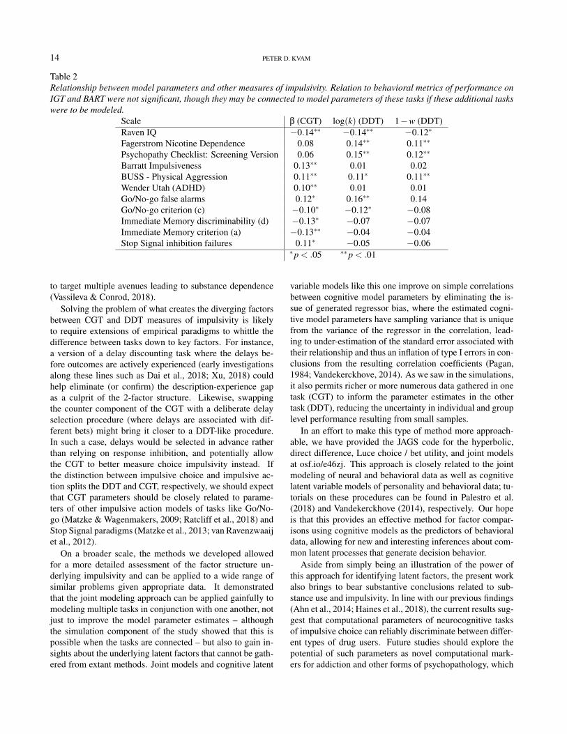
In general, the β parameter from the CGT is more closelyrelated to performance on the Barratt Impulsiveness Scaleas well as behavioral measures of response inhibition on theGo/No-go task and Stop Signal paradigms. Waiting for thetimer to tick over in the Cambridge gambling tasks requiresthe ability to inhibit making a response until the target betproportion is reached. A failure to inhibit an early responsewill naturally result in higher estimates of β. This may natu-rally be the reason that it is related to inhibition failures in theStop Signal paradigm as well as the higher rate of responsesin the Go/No-go paradigm (resulting in a higher rate of falsealarms and hits, and thus a shift in the criterion measure c).This would suggest that it is more closely related to the im-pulsive action dimension of impulsivity, rather than the im-pulsive choice dimension normally associated with temporaldiscounting.

Conversely, the k parameter (and w) are more closely re-lated to measures of externalizing issues like aggression andpsychopathy, while both tasks are negatively related to RavenIQ. This lines up closely with the observation of Reynolds etal. (2006), who broke down impulsivity into a response in-hibition component – related to performance on Stop Signal(Verbruggen & Logan, 2008) and Go/No-Go tasks – and amore long-term impulsivity that impacts performance on theDDT and BART tasks and self-report measures like the Bar-ratt scale. In terms of the dimensions of impulsivity, theseresults suggest that the DDT parameter lines up more closelywith impulsive choice measures, whereas the CGT parame-ter lines up with impulsive action or response disinhibition(Hamilton, Mitchell, et al., 2015; Hamilton, Littlefield, et al.,2015; MacKillop et al., 2016). However, the DDT parameterseems to line up somewhat with self-report measures as well,suggesting that it may be related to both impulsive choice andimpulsive personality dimensions – or possibly that these two

dimensions are more closely related to one another than toimpulsive action.

Discussion

Given the differences in task structure, it may not be toosurprising that the delay discounting task and Cambridgegambling task actually appear to measure separate dimen-sions of impulsivity. Much like the diverging results betweendescribed and experienced outcomes in risky choice, it maybe the case that there is an analogous “description-experiencegap” (Hertwig et al., 2018; Hertwig & Erev, 2009; Wulff etal., 2018) in impulsive choice as well. Such a gap wouldnaturally manifest in differences in performance between thedelay discounting task, where the delays are not experiencedin real time between trials of choices (though of course thesedecisions may be played out following the experiment), andthe Cambridge gambling task, where the delays are expe-rienced on each and every trial before a bet can be made.While the type of analysis developed here is informative, itcannot determine whether these differences reflect a true dif-ference in the tasks measuring different latent constructs, orinstead reflect mainly the contribution of learning processesto performance (Haines et al., submitted).

Of course, experience versus description is not the onlydifference between the tasks. The delay discounting task usesdelays that are typically on the order of weeks or months,which is much longer than the 0-25 second time scale im-plemented for making bets in the Cambridge gambling task.The difference in performance may instead arise because theDDT relies on long-term planning whereas the CGT relieson inhibiting more immediate responses in a similar fashionto Go/No-go and Stop signal tasks (Reynolds et al., 2006).These two tasks may therefore be measuring separate dimen-sions of impulsivity: the CGT appears to be related to impul-sive action, while delay discounting is related to trait-levelcharacteristics like impulsive personality and by definitionrelated to impulsive choice (MacKillop et al., 2016). If de-lay discounting is indeed a trait-level characteristic (Odum,2011), this would explain why it tends to be more stable overtime (Simpson & Vuchinich, 2000) and its relation to self-report measures of impulsivity (like the BIS or UPPS) thatare designed to assess personality.

Impulsivity is best understood as a multidimensional con-struct that affects many different cognitive processes con-tributing to substance use outcomes and consisting of bothstate and trait components (Isles et al., 2018; Vassileva &Conrod, 2018). Having multiple assessment procedures thatengage cognitive processes related to long-term planning orresponse inhibition allows us to uncover their unique andspecific contributions to disordered decision making. Theobservation that they both underlie health outcomes relatedto psychopathy and substance use disorders (Ahn & Vas-sileva, 2016) suggest that intervention strategies may need

14 PETER D. KVAM

Table 2Relationship between model parameters and other measures of impulsivity. Relation to behavioral metrics of performance onIGT and BART were not significant, though they may be connected to model parameters of these tasks if these additional taskswere to be modeled.

Scale β (CGT) log(k) (DDT) 1−w (DDT)Raven IQ −0.14∗∗ −0.14∗∗ −0.12∗

Fagerstrom Nicotine Dependence 0.08 0.14∗∗ 0.11∗∗

Psychopathy Checklist: Screening Version 0.06 0.15∗∗ 0.12∗∗

Barratt Impulsiveness 0.13∗∗ 0.01 0.02BUSS - Physical Aggression 0.11∗∗ 0.11∗ 0.11∗∗

Wender Utah (ADHD) 0.10∗∗ 0.01 0.01Go/No-go false alarms 0.12∗ 0.16∗∗ 0.14Go/No-go criterion (c) −0.10∗ −0.12∗ −0.08Immediate Memory discriminability (d) −0.13∗ −0.07 −0.07Immediate Memory criterion (a) −0.13∗∗ −0.04 −0.04Stop Signal inhibition failures 0.11∗ −0.05 −0.06

∗p < .05 ∗∗p < .01

to target multiple avenues leading to substance dependence(Vassileva & Conrod, 2018).

Solving the problem of what creates the diverging factorsbetween CGT and DDT measures of impulsivity is likelyto require extensions of empirical paradigms to whittle thedifference between tasks down to key factors. For instance,a version of a delay discounting task where the delays be-fore outcomes are actively experienced (early investigationsalong these lines such as Dai et al., 2018; Xu, 2018) couldhelp eliminate (or confirm) the description-experience gapas a culprit of the 2-factor structure. Likewise, swappingthe counter component of the CGT with a deliberate delayselection procedure (where delays are associated with dif-ferent bets) might bring it closer to a DDT-like procedure.In such a case, delays would be selected in advance ratherthan relying on response inhibition, and potentially allowthe CGT to better measure choice impulsivity instead. Ifthe distinction between impulsive choice and impulsive ac-tion splits the DDT and CGT, respectively, we should expectthat CGT parameters should be closely related to parame-ters of other impulsive action models of tasks like Go/No-go (Matzke & Wagenmakers, 2009; Ratcliff et al., 2018) andStop Signal paradigms (Matzke et al., 2013; van Ravenzwaaijet al., 2012).

On a broader scale, the methods we developed allowedfor a more detailed assessment of the factor structure un-derlying impulsivity and can be applied to a wide range ofsimilar problems given appropriate data. It demonstratedthat the joint modeling approach can be applied gainfully tomodeling multiple tasks in conjunction with one another, notjust to improve the model parameter estimates – althoughthe simulation component of the study showed that this ispossible when the tasks are connected – but also to gain in-sights about the underlying latent factors that cannot be gath-ered from extant methods. Joint models and cognitive latent

variable models like this one improve on simple correlationsbetween cognitive model parameters by eliminating the is-sue of generated regressor bias, where the estimated cogni-tive model parameters have sampling variance that is uniquefrom the variance of the regressor in the correlation, lead-ing to under-estimation of the standard error associated withtheir relationship and thus an inflation of type I errors in con-clusions from the resulting correlation coefficients (Pagan,1984; Vandekerckhove, 2014). As we saw in the simulations,it also permits richer or more numerous data gathered in onetask (CGT) to inform the parameter estimates in the othertask (DDT), reducing the uncertainty in individual and grouplevel performance resulting from small samples.

In an effort to make this type of method more approach-able, we have provided the JAGS code for the hyperbolic,direct difference, Luce choice / bet utility, and joint modelsat osf.io/e46zj. This approach is closely related to the jointmodeling of neural and behavioral data as well as cognitivelatent variable models of personality and behavioral data; tu-torials on these procedures can be found in Palestro et al.(2018) and Vandekerckhove (2014), respectively. Our hopeis that this provides an effective method for factor compar-isons using cognitive models as the predictors of behavioraldata, allowing for new and interesting inferences about com-mon latent processes that generate decision behavior.

Aside from simply being an illustration of the power ofthis approach for identifying latent factors, the present workalso brings to bear substantive conclusions related to sub-stance use and impulsivity. In line with our previous findings(Ahn et al., 2014; Haines et al., 2018), the current results sug-gest that computational parameters of neurocognitive tasksof impulsive choice can reliably discriminate between differ-ent types of drug users. Future studies should explore thepotential of such parameters as novel computational mark-ers for addiction and other forms of psychopathology, which

JOINT CLINICAL MODELING 15

may help refine addiction phenotypes and develop more rig-orous models of addiction.

References

Ahn, W. Y., Dai, J., Vassileva, J., Busemeyer, J. R., & Stout,J. C. (2016). Computational modeling for addictionmedicine: from cognitive models to clinical applications.In Progress in brain research (Vol. 224, pp. 53–65). Else-vier.

Ahn, W.-Y., Ramesh, D., Moeller, F. G., & Vassileva, J.(2016). Utility of machine-learning approaches to iden-tify behavioral markers for substance use disorders: im-pulsivity dimensions as predictors of current cocaine de-pendence. Frontiers in psychiatry, 7, 34.

Ahn, W.-Y., Vasilev, G., Lee, S.-H., Busemeyer, J. R.,Kruschke, J. K., Bechara, A., & Vassileva, J. (2014).Decision-making in stimulant and opiate addicts in pro-tracted abstinence: evidence from computational model-ing with pure users. Frontiers in Psychology, 5, 849.

Ahn, W.-Y., & Vassileva, J. (2016). Machine-learning iden-tifies substance-specific behavioral markers for opiate andstimulant dependence. Drug and alcohol dependence,161, 247–257.

Ainslie, G. W. (1974). Impulse control in pigeons 1. Journalof the experimental analysis of behavior, 21(3), 485–489.

Ainslie, G. W. (1975). Specious reward: a behavioral the-ory of impulsiveness and impulse control. Psychologicalbulletin, 82(4), 463.

Ainslie, G. W., & Haslam, N. (1992). Hyperbolic discount-ing. Russell Sage Foundation.

Bechara, A., Damasio, A. R., Damasio, H., & Anderson,S. W. (1994). Insensitivity to future consequences follow-ing damage to human prefrontal cortex. Cognition, 50(1-3), 7–15.

Bickel, W. K., Jarmolowicz, D. P., Mueller, E. T., Koffarnus,M. N., & Gatchalian, K. M. (2012). Excessive discount-ing of delayed reinforcers as a trans-disease process con-tributing to addiction and other disease-related vulnerabil-ities: emerging evidence. Pharmacology & therapeutics,134(3), 287–297.

Bickel, W. K., Johnson, M. W., Koffarnus, M. N., MacKil-lop, J., & Murphy, J. G. (2014). The behavioral economicsof substance use disorders: reinforcement pathologies andtheir repair. Annual review of clinical psychology, 10,641–677.

Bickel, W. K., & Marsch, L. A. (2001). Toward a behav-ioral economic understanding of drug dependence: delaydiscounting processes. Addiction, 96(1), 73–86.

Bickel, W. K., Mellis, A. M., Snider, S. E., Moody, L., Stein,J. S., & Quisenberry, A. J. (2016). Novel therapeuticsfor addiction: Behavioral economic and neuroeconomicapproaches. Current treatment options in psychiatry, 3(3),277–292.

Bickel, W. K., Yi, R., Landes, R. D., Hill, P. F., & Baxter,C. (2011). Remember the future: working memory train-ing decreases delay discounting among stimulant addicts.Biological psychiatry, 69(3), 260–265.

Busemeyer, J. R., & Stout, J. C. (2002). A contribution ofcognitive decision models to clinical assessment: decom-posing performance on the bechara gambling task. Psy-chological assessment, 14(3), 253.

Buss, A. H., & Warren, W. (2000). Aggression question-naire:(aq). manual. Western Psychological Services.

Camerer, C. (1999). Behavioral economics: Reunifyingpsychology and economics. Proceedings of the NationalAcademy of Sciences, 96(19), 10575–10577.

Cheng, J., & González-Vallejo, C. (2016). Attribute-wise vs.alternative-wise mechanism in intertemporal choice: Test-ing the proportional difference, trade-off, and hyperbolicmodels. Decision, 3(3), 190.

Chung, S.-H., & Herrnstein, R. J. (1967). Choice and delayof reinforcement I. Journal of the Experimental Analysisof Behavior, 10(1), 67–74.

Conrod, P. J., Castellanos-Ryan, N., & Strang, J. (2010).Brief, personality-targeted coping skills interventions andsurvival as a non–drug user over a 2-year period duringadolescence. Archives of general psychiatry, 67(1), 85–93.

Dai, J., & Busemeyer, J. R. (2014). A probabilistic, dynamic,and attribute-wise model of intertemporal choice. Journalof Experimental Psychology: General, 143(4), 1489.

Dai, J., Pachur, T., Pleskac, T., & Hertwig, R. (2018).What the future holds and when a description-experiencegap in intertemporal choice. Preprint retrived frompsyarxiv.com/grwye.

Daugherty, J. R., & Brase, G. L. (2010). Taking time to behealthy: Predicting health behaviors with delay discount-ing and time perspective. Personality and Individual dif-ferences, 48(2), 202–207.

Dawe, S., & Loxton, N. J. (2004). The role of impulsivityin the development of substance use and eating disorders.Neuroscience & Biobehavioral Reviews, 28(3), 343–351.

16 PETER D. KVAM

De Wit, H. (2009). Impulsivity as a determinant and con-sequence of drug use: a review of underlying processes.Addiction biology, 14(1), 22–31.

Donohew, L., Zimmerman, R., Cupp, P. S., Novak, S.,Colon, S., & Abell, R. (2000). Sensation seeking, im-pulsive decision-making, and risky sex: Implications forrisk-taking and design of interventions. Personality andindividual differences, 28(6), 1079–1091.

Dougherty, D. M., Marsh, D. M., & Mathias, C. W. (2002).Immediate and delayed memory tasks: a computerizedbehavioral measure of memory, attention, and impulsiv-ity. Behavior research methods, instruments, & comput-ers, 34(3), 391–398.

Dougherty, D. M., Mathias, C. W., Marsh, D. M., & Jagar,A. A. (2005). Laboratory behavioral measures of impul-sivity. Behavior Research Methods, 37(1), 82–90.

Fridberg, D. J., Queller, S., Ahn, W.-Y., Kim, W., Bishara,A. J., Busemeyer, J. R., . . . Stout, J. C. (2010). Cog-nitive mechanisms underlying risky decision-making inchronic cannabis users. Journal of mathematical psychol-ogy, 54(1), 28–38.

Haines, N., Kvam, P. D., & Turner, B. M. (submitted).Bridging the description-experience gap in risky decision-making: Asymmetric learning of positive and negativepredictions errors as a causal mechanism. Manuscript un-der review.

Haines, N., Vassileva, J., & Ahn, W.-Y. (2018). Theoutcome-representation learning model: A novel rein-forcement learning model of the iowa gambling task. Cog-nitive science, 42(8), 2534–2561.

Hamilton, K. R., Littlefield, A. K., Anastasio, N. C., Cun-ningham, K. A., Fink, L. H., Wing, V. C., . . . others(2015). Rapid-response impulsivity: Definitions, mea-surement issues, and clinical implications. PersonalityDisorders: Theory, Research, and Treatment, 6(2), 168.

Hamilton, K. R., Mitchell, M. R., Wing, V. C., Balodis, I. M.,Bickel, W. K., Fillmore, M., . . . others (2015). Choiceimpulsivity: Definitions, measurement issues, and clinicalimplications. Personality Disorders: Theory, Research,and Treatment, 6(2), 182.

Hare, R. D. (2003). The psychopathy checklist–revised.

Hart, S. D., Cox, D. N., & Hare, R. D. (1995). Hare psy-chopathy checklist: Screening version (pcl: Sv). Multi-Heath Systems.

Hau, R., Pleskac, T. J., Kiefer, J., & Hertwig, R. (2008).The description–experience gap in risky choice: The role

of sample size and experienced probabilities. Journal ofBehavioral Decision Making, 21(5), 493–518.

Heathcote, A., Brown, S. D., & Wagenmakers, E.-J. (2015).An introduction to good practices in cognitive modeling.In An introduction to model-based cognitive neuroscience(pp. 25–48). Springer.

Heatherton, T. F., Kozlowski, L. T., Frecker, R. C., &FAGERSTROM, K.-O. (1991). The fagerström test fornicotine dependence: a revision of the fagerstrom toler-ance questionnaire. British journal of addiction, 86(9),1119–1127.

Hertwig, R., & Erev, I. (2009). The description–experiencegap in risky choice. Trends in Cognitive Sciences, 13(12),517–523. doi: 10.1016/j.tics.2009.09.004

Hertwig, R., Wulff, D. U., & Mata, R. (2018). Threegaps and what they may mean for risk preference. Philo-sophical Transactions of the Royal Society B, 374(1766),20180140.

Isles, A. R., Winstanley, C. A., & Humby, T. (2018).Risk taking and impulsive behaviour: fundamental discov-eries, theoretical perspectives and clinical implications(Vol. 374). The Royal Society.

Jeffreys, H. (1961). The theory of probability. OUP Oxford.

Kirby, K. N., & Herrnstein, R. J. (1995). Preference reversalsdue to myopic discounting of delayed reward. Psycholog-ical Science, 6(2), 83–89.

Kirby, K. N., & Marakovic, N. N. (1995). Modeling my-opic decisions: Evidence for hyperbolic delay-discountingwithin subjects and amounts. Organizational Behaviorand Human decision processes, 64(1), 22–30.

Kirby, K. N., & Marakovic, N. N. (1996). Delay-discountingprobabilistic rewards: Rates decrease as amounts increase.Psychonomic bulletin & review, 3(1), 100–104.

Kirby, K. N., Petry, N. M., & Bickel, W. K. (1999). Heroinaddicts have higher discount rates for delayed rewards thannon-drug-using controls. Journal of Experimental psy-chology: general, 128(1), 78.

Konova, A. B., Lopez-Guzman, S., Urmanche, A., Ross, S.,Louie, K., Rotrosen, J., & Glimcher, P. W. (2019). Com-putational markers of risky decision-making for identifica-tion of temporal windows of vulnerability to opioid use ina real-world clinical setting. JAMA psychiatry.

Kruschke, J. (2014). Doing bayesian data analysis: A tuto-rial with R, JAGS, and STAN. Academic Press.

JOINT CLINICAL MODELING 17

Lane, S. D., Moeller, F. G., Steinberg, J. L., Buzby, M., &Kosten, T. R. (2007). Performance of cocaine dependentindividuals and controls on a response inhibition task withvarying levels of difficulty. The American journal of drugand alcohol abuse, 33(5), 717–726.

Lee, M. D., & Wagenmakers, E.-J. (2014). Bayesian cogni-tive modeling: A practical course. Cambridge universitypress.

Lejuez, C. W., Aklin, W. M., Jones, H. A., Richards, J. B.,Strong, D. R., Kahler, C. W., & Read, J. P. (2003). The bal-loon analogue risk task (bart) differentiates smokers andnonsmokers. Experimental and clinical psychopharma-cology, 11(1), 26.

Lejuez, C. W., Read, J. P., Kahler, C. W., Richards, J. B.,Ramsey, S. E., Stuart, G. L., . . . Brown, R. A. (2002).Evaluation of a behavioral measure of risk taking: the bal-loon analogue risk task (bart). Journal of ExperimentalPsychology: Applied, 8(2), 75.

Levenson, M. R., Kiehl, K. A., & Fitzpatrick, C. M. (1995).Assessing psychopathic attributes in a noninstitutionalizedpopulation. Journal of personality and social psychology,68(1), 151.

Luce, R. D. (1959). Individual choice behavior: A theoreti-cal analysis. John Wiley and Sons.

MacKillop, J., Amlung, M. T., Few, L. R., Ray, L. A., Sweet,L. H., & Munafò, M. R. (2011). Delayed reward discount-ing and addictive behavior: a meta-analysis. Psychophar-macology, 216(3), 305–321.

MacKillop, J., Weafer, J., Gray, J. C., Oshri, A., Palmer, A.,& de Wit, H. (2016). The latent structure of impulsivity:impulsive choice, impulsive action, and impulsive person-ality traits. Psychopharmacology, 233(18), 3361–3370.

Matzke, D., Dolan, C. V., Logan, G. D., Brown, S. D., &Wagenmakers, E.-J. (2013). Bayesian parametric estima-tion of stop-signal reaction time distributions. Journal ofExperimental Psychology: General, 142(4), 1047.

Matzke, D., & Wagenmakers, E.-J. (2009). Psychologicalinterpretation of the ex-gaussian and shifted wald parame-ters: A diffusion model analysis. Psychonomic bulletin &review, 16(5), 798–817.

Mazur, J. E. (1987). An adjusting procedure for studying de-layed reinforcement. Commons, ML.; Mazur, JE.; Nevin,JA, 55–73.

Moeller, F. G., Barratt, E. S., Dougherty, D. M., Schmitz,J. M., & Swann, A. C. (2001). Psychiatric aspects of im-pulsivity. American journal of psychiatry, 158(11), 1783–1793.

Odum, A. L. (2011). Delay discounting: I’m ak, you’re ak.Journal of the experimental analysis of behavior, 96(3),427–439.

Pagan, A. (1984). Econometric issues in the analysis ofregressions with generated regressors. International Eco-nomic Review, 221–247.

Palestro, J. J., Bahg, G., Sederberg, P. B., Lu, Z.-L., Steyvers,M., & Turner, B. M. (2018). A tutorial on joint models ofneural and behavioral measures of cognition. Journal ofMathematical Psychology, 84, 20–48.

Patton, J. H., Stanford, M. S., & Barratt, E. S. (1995). Fac-tor structure of the barratt impulsiveness scale. Journal ofclinical psychology, 51(6), 768–774.

Petry, N. M. (2001). Substance abuse, pathological gam-bling, and impulsiveness. Drug and alcohol dependence,63(1), 29–38.

Plummer, M., et al. (2003). JAGS: A program for analysis ofbayesian graphical models using Gibbs sampling. In Pro-ceedings of the 3rd international workshop on distributedstatistical computing (Vol. 124, p. 10).

Ratcliff, R., Huang-Pollock, C., & McKoon, G. (2018).Modeling individual differences in the go/no-go task witha diffusion model. Decision, 5(1), 42.

Raven, J. (2000). The raven’s progressive matrices: changeand stability over culture and time. Cognitive psychology,41(1), 1–48.

Reynolds, B. (2006). A review of delay-discounting researchwith humans: relations to drug use and gambling. Be-havioural pharmacology, 17(8), 651–667.

Reynolds, B., Ortengren, A., Richards, J. B., & de Wit, H.(2006). Dimensions of impulsive behavior: Personalityand behavioral measures. Personality and individual dif-ferences, 40(2), 305–315.

Rogers, R. D., Everitt, B., Baldacchino, A., Blackshaw, A.,Swainson, R., Wynne, K., . . . others (1999). Dissocia-ble deficits in the decision-making cognition of chronicamphetamine abusers, opiate abusers, patients with focaldamage to prefrontal cortex, and tryptophan-depleted nor-mal volunteers: evidence for monoaminergic mechanisms.Neuropsychopharmacology, 20(4), 322–339.

Romeu, R. J., Haines, N., Ahn, W.-Y., Busemeyer, J. R., &Vassileva, J. (2019). A computational model of the cam-bridge gambling task with applications to substance usedisorders. Drug and alcohol dependence, 107711.

18 PETER D. KVAM

Shiffrin, R., Lee, M., Kim, W., & Wagenmakers, E.-J. (2008). A Survey of Model Evaluation Ap-proaches With a Tutorial on Hierarchical Bayesian Meth-ods. Cognitive Science: A Multidisciplinary Journal,32(8), 1248–1284. Retrieved from http://doi.wiley.com/10.1080/03640210802414826 doi: 10.1080/03640210802414826

Simpson, C. A., & Vuchinich, R. E. (2000). Reliabilityof a measure of temporal discounting. The PsychologicalRecord, 50(1), 3–16.

Steyvers, M. (2011). Matjags 1.3: A matlab interface forjags.

Turner, B. M. (2015). Constraining cognitive abstractionsthrough Bayesian modeling. In B. U. Forstmann & E.-J. Wagenmakers (Eds.), An introduction to model-basedcognitive neuroscience (p. 199-220). New York: Springer.

Turner, B. M., Forstmann, B. U., Wagenmakers, E.-J.,Brown, S. D., Sederberg, P. B., & Steyvers, M. (2013). ABayesian framework for simultaneously modeling neuraland behavioral data. NeuroImage, 72, 193–206.

Turner, B. M., Rodriguez, C. A., Norcia, T. M., McClure,S. M., & Steyvers, M. (2016). Why more is better: Si-multaneous modeling of eeg, fmri, and behavioral data.Neuroimage, 128, 96–115.

Turner, B. M., Van Maanen, L., & Forstmann, B. U. (2015).Combining cognitive abstractions with neurophysiology:The neural drift diffusion model. Psychological Review,122, 312-336.

Turner, B. M., Wang, T., & Merkle, E. C. (2017). Factor anal-ysis linking functions for simultaneously modeling neuraland behavioral data. NeuroImage, 153, 28–48.

Vandekerckhove, J. (2014). A cognitive latent variable modelfor the simultaneous analysis of behavioral and personalitydata. Journal of Mathematical Psychology, 60, 58–71.

van Ravenzwaaij, D., van der Maas, H. L., & Wagenmakers,E.-J. (2012). Optimal decision making in neural inhibitionmodels. Psychological Review, 119(1), 201.

Vassileva, J., Ahn, W.-Y., Weber, K. M., Busemeyer, J. R.,Stout, J. C., Gonzalez, R., & Cohen, M. H. (2013). Com-putational modeling reveals distinct effects of hiv and his-tory of drug use on decision-making processes in women.PloS one, 8(8), e68962.

Vassileva, J., & Conrod, P. J. (2018). Impulsivities andaddictions: a multidimensional integrative framework in-forming assessment and interventions for substance usedisorders. Philosophical Transactions of the Royal SocietyB, 374(1766), 20180137.

Vassileva, J., Long, E., Kaneva, R., Psederska, E., Bozgunov,K., Nedelchev, D., & Vasilev, G. (2018). F272. psychiatricand impulsivity dimensions as common and specific can-didate endophenotypes for heroin and amphetamine de-pendence. Biological Psychiatry, 83(9), S345.

Verbruggen, F., & Logan, G. D. (2008). Response inhibitionin the stop-signal paradigm. Trends in cognitive sciences,12(11), 418–424.

Verdinelli, I., & Wasserman, L. (1995). Computing bayesfactors using a generalization of the savage-dickey den-sity ratio. Journal of the American Statistical Association,90(430), 614–618.

Wagenmakers, E. J., Lodewyckx, T., Kuriyal, H., & Gras-man, R. (2010). Bayesian hypothesis testing for psychol-ogists: A tutorial on the Savage-Dickey method. Cogni-tive Psychology, 60(3), 158–189. doi: 10.1016/j.cogpsych.2009.12.001

Ward, M. F. (1993). The wender utah rating scale: An aid inthe retrospective. American Journal of Psychiatry, 1(50),885.

Whiteside, S. P., & Lynam, D. R. (2001). The five factormodel and impulsivity: Using a structural model of per-sonality to understand impulsivity. Personality and indi-vidual differences, 30(4), 669–689.

Wulff, D. U., Mergenthaler-Canseco, M., & Hertwig, R.(2018). A meta-analytic review of two modes of learn-ing and the description-experience gap. Psychological bul-letin, 144(2), 140.

Xu, P. (2018). Examining the description-experienced gapin time discounting and its possible mechanisms (Unpub-lished doctoral dissertation). Ohio University.

Zois, E., Kortlang, N., Vollstädt-Klein, S., Lemenager, T.,Beutel, M., Mann, K., & Fauth-Bühler, M. (2014).Decision-making deficits in patients diagnosed with dis-ordered gambling using the cambridge gambling task: theeffects of substance use disorder comorbidity. Brain andbehavior, 4(4), 484–494.

Zuckerman, M., Kolin, E. A., Price, L., & Zoob, I. (1964).Development of a sensation-seeking scale. Journal of con-sulting psychology, 28(6), 477.

Appendix A: Direct difference model of delaydiscounting

One concern with connecting the parameters of two sepa-rate cognitive models is whether the conclusions of the analy-sis depend heavily on the models themselves. We tested sev-eral variants of the hyperbolic and Luce choice/bet models,

JOINT CLINICAL MODELING 19

arriving on the ones used above primarily because they pro-vided the best mix of recoverability and completeness. How-ever, we also tested an alternative to the hyperbolic discount-ing model, the direct difference model (Dai & Busemeyer,2014; Cheng & González-Vallejo, 2016). This model positsthat people compare options in the delay discounting task bycomparing them on individual attributes. The direct differ-ence model computes the difference between alternatives ona particular attribute – such as delay – and then combines thedifferences between item attributes into an overall differencein subjective value. This is referred to as an attribute-wisemodel, which sits in contrast to the hyperbolic discountingmodel and other alternative-wise models, which compute anoverall item value by taking the reward value and discountingits subjective value according to the delay associated with it.

The direct difference model uses three main parameters.The first parameter υ describes the utility (u(x)) associatedwith different bets (x) as

u(x) = xυ (11)

Similarly, the second parameter ν describes the utility(v(t)) associated with different delays (t):

v(t) = tν (12)

Like most utility functions, both of these consist of apower function with a single free parameter (υ or ν), yieldinga concave mapping from reward amount or delay to subjec-tive value. Once the values of each attribute are computed forboth alternatives, they are contrasted against one another. Fortwo delayed prospects (x1, t1) and (x2, t2), this yields a utilitydifference for rewards u(x1)− u(x2) and a utility differencefor delays v(x1)− v(x2). The overall difference in subjectivevalue is computed by putting a relative weight on each at-tribute. This is done by multiplying a free weight parameterw by the reward utility difference, and its inverse (1−w) bythe delay utility difference. For the comparison between alarger later option (xL,tL) and a smaller sooner option (xS,tS),this gives an overall difference in subjective value d.

d = w(xυL− xυ

S)− (1−w)(tνL− tν

S ) (13)

The direct difference model predicts choice variability as afunction of these three parameters as well. We use a randomutility implementation of the model, where the difference insubjective value is associated with an accompanying vari-ance, which creates random differences in choice behaviorfrom selection to selection. The square root of this variance(the standard deviation) is given as σ.

σ =√

w · (xL− xS)2 +(1−w) · (tL− tS)2−d2 (14)

The probability of selecting the larger later option is afunction of d and σ:

Figure 9. Individual estimates of w in the direct differencemodel of the DDT (x-axis) and β in the model of the CGT,along with the strength of relationship between them (colorcorresponds to lifetime substance use classification). The re-sult when models are fit jointly (1-factor) is shown on the leftand fit separately (2-factor) on the right.

pL = Φ(dσ) (15)

Here, Φ is the cumulative distribution function for a stan-dard normal random variable. The model can then be fit tothe data by estimating the choice probabilities as a functionof w, υ, and ν. While there isn’t a parameter that directlydescribes temporal discounting, the w parameter does con-trol the relative weight assigned to reward and delay infor-mation. A smaller value of w results in more weight on delayinformation, and a larger w results in more weight on rewardinformation. A more impulsive participant who discounts re-wards heavily should therefore appear to pay more attentionto delay information, resulting in a smaller value for w. Asa result, we use 1−w as the measure of impulsivity in thedirect difference model of the DDT.

Individual Estimates

For the direct difference model, we can repeat the joint (1-factor) and separate (2-factor) modeling analyses. Because wis on a bounded scale of [0,1] and β is on an unbounded scale,we set the transformation from Imp (the latent impulsivityfactor) to w as a logistic mapping

w =1

1+ exp(−Imp)(16)

This is in place of the exponential mapping used for thehyperbolic discounting parameter k. All other settings werethe same for the CGT side of the joint model.

The results of the individual-level estimates for 1−w andβ are shown in Figure 9. As before, blue circles are estimatesfor controls, red diamonds are heroin users, yellow squaresare amphetamine users, and purple triangles are estimates forpolysubstance users. As shown in the left panel, there are notparticularly strong covariances between 1−w and β for anyof the substance use groups, reflected in the relatively flat

20 PETER D. KVAM

Figure 10. Group-level mean estimates of w in the directdifference model of the DDT (x-axis) and β in the model ofthe CGT. The result when models are fit jointly (1-factor) isshown on the left, and fit separately (2-factor) on the right.Error bars correspond to 95% highest density intervals ongroup-level estimates.

slopes for the lines depicting the average relationship. Aswith the hyperbolic discounting joint model, the direct differ-ence joint model (left side of Figure 9) accentuated the slopesof the relationships between the two impulsivity parameters,but even these were not particularly strong.

Group level estimates

The effects of modeling the DDT and CGT as a 1-factorversus 2-factor model can be observed in the group-level es-timates of the w and β parameters as well, shown in Figure10.

As with the hyperbolic discounting joint model, constrain-ing both w and β using a common Impulsivity factor (1-factormodel, left of Figure 10) primarily introduces uncertaintyinto the posterior of the estimates of β when compared withfitting the models when this relationship is fixed at bCGT = 0(2 factor model, right of Figure 10).

Interestingly, the direct difference model seems to be bet-ter at capturing differences between substance use groupswhen it comes to delay discounting behavior: Controls weremuch lower than substance users in terms of mean estimatesof w. However, the direct difference model generally fitworse than the hyperbolic discounting model on this data set.The deviance information criterion [DIC], which indexes thequality of model fit with a penalty for a greater number ofparameters (a lower DIC is considered better), was consis-tently lower for the hyperbolic model: the hyperbolic modelfit with DIC values of 1846.4, 726.4, 865.6, and 1180.0 forthe control, heroin, amphetamine, and polysubstance groups,respectively; while the direct difference model fit with DICvalues of 2212.4, 889.0, 910.7, and 1292.4 for the same re-spective groups. This leaves a conundrum which will cer-tainly not be answered here, which is whether a model that isbetter at predicting substance use outcomes but with inferiorquality of model fit is preferable to a model that is worseat predicting substance use but has a higher quality of fit.

Figure 11. Diagram of Savage-Dickey Bayes factor for di-rect difference model, comparing prior (lighter color) againstposterior (darker color) distributions on the degree of supportfor an estimate of zero.

This is certainly an issue that should be addressed in futurecomparisons between temporal discounting models.

Bayes factor comparison

Finally, we can repeat the comparison between 1-factorand 2-factor models for the direct difference model. As be-fore, we compare the prior likelihood of bCGT = 0 (before itis updated with the data) against the posterior likelihood ofbCGT = 0 (after it is updated with the data) by computing theratio from Equation 10. A value greater than 1 indicates evi-dence in favor of the 2-factor model, while a value less than1 indicates evidence against it (instead favoring the 1-factormodel).

The results of the Bayes factor analysis for the direct dif-ference model are shown in Figure 11. While the evidencein favor of the 2-factor model is not quite as strong as it waswith the hyperbolic discounting model – most evidence fallsin the “weak” (1-3) to “moderate” strength range (3-10) – the2-factor model is still favored over the 1-factor model for allsubstance use groups. It is worth noting that the prior herewas somewhat more constrained relative to the posterior; asshown in the Savage-Dickey diagram for the control group(top left), even though the posterior distribution is centeredright at zero, the evidence in favor of the 2-factor model isnot as strong as in the analysis of the hyperbolic model. Thisis therefore largely due to the amount of uncertainty in theposterior relative to the prior, rather than particularly strongevidence against a value of bCGT = 0.

The relation of 1−w to the health outcome measures canbe seen in Table 2. Its predictions are generally in line withthe log(k) measure from the hyperbolic model, although ingeneral it is a weaker predictor of most outcomes.

JOINT CLINICAL MODELING 21

Overall, using the direct difference model does not resultin substantial changes in the conclusions of the study. It tendsto better assess differences between groups, as w discrimi-nates between substance users and non-substance users betterthan k, but using this model still results in evidence favoringthe 2-factor model of impulsivity.

Formal specification of the models

In order to make the models more widely accessible, wehave provided the JAGS code for all of the ones listed here– including 1- and 2-factor models as well as hyperbolic anddirect difference models – at osf.io/e46zj/. For those who areunable or prefer not to read this code, we outline the contenthere for the joint model, starting with the ‘highest-order’ im-pulsivity construct Imp, whose prior is normally distributed(using mean, SD as the parameters of the normal, as opposedto mean, precision as in JAGS):

Imp∼ N(0,10) (17)

The values of log(k) and β for each individual are linearfunctions of the impulsivity value (plus error), with the coef-ficient mapping it onto log(k) set to one, to fix the scale ofthe model and ensure identifiability.

log(k) = Imp+N(0,ζDDT )

β = bCGT · Imp+N(b0,ζCGT )

The priors for each of the other individual-level parame-ters were set to be uninformative with a different mean foreach group, as normal distributions N(0,100) (for probabil-ity sensitivity α and bet variability γ in the CGT, and choicevariability m in the DDT) or uniform distributions (for thecolor bias c in the CGT). The prior for bCGT was also nor-mal, N(0,10), and all precision parameters for group levelpriors were set to be uninformative as a gamma distribu-tion Gamma(.001, .001) (in shape-rate form). In the directdifference model, the variability parameter σ was set withan exponentially distributed prior Exp(.01) (in rate form).The likelihood of the data was then given as a function ofthese parameters. For the hyperbolic model, the likelihoodof choosing the LL alternative is

Pr(LL) =1

1+ exp(−m ·(

xLL1+k·tLL

− xSS1+k·tSS

))

.

The Cambridge gambling task had two different data out-puts. The first of these was the proportion of times the redboxes (vs blue) were chosen, which is given as a function ofthe number of red boxes NR and the free parameters for colorbias c and choice variability α.

Pr(R) =c ·Nα

Rc ·Nα

R +(1− c) · (10−NR)α

The prediction for making a particular bet depended onwhether the ticker was ascending or descending as well aswhether the initial choice was correct, which is designated asPr(C) such that Pr(C) = Pr(R) ·NR/10+(1−Pr(R))(10−NR)/10). Given the time associated with a particular bet TB,the number of current points the participant had, and the pa-rameters γ and β, the probability of choosing a bet bi was

Pr(B= bi|C)=exp(γ · pts · (Pr(C) · (1+bi)+(1−Pr(C)) · (1−bi))−β ·Tbi)

5∑j=1

exp(γ · pts · (Pr(C) · (1+b j)+(1−Pr(C)) · (1−b j))−β ·Tb j)

.

Naturally, the bet had to be conditioned on the choice inorder to ensure that the sum across all possible combina-tions of color choice and succeeding bet added up to one.Using these likelihoods and priors, the posterior distributionof each of the parameters was estimated via Markov chainMonte Carlo sampling in JAGS (Plummer et al., 2003), in-terfacing with MATLAB via matjags (Steyvers, 2011). Typi-cally, the models were run for 4 chains of 4000 samples with500 burn-in samples and inspected for conversion using ther statistic and visual inspection of the sequences of samples.To compare the posterior against the prior distribution (usedfor the Savage-Dickey Bayes factor), we passed a standardGaussian kernel density estimator over the collection of pos-terior samples and compared the height of this distributionat zero against that of the prior (which was known from thedistribution specified in Equation 17. The posterior sampleswere also used to generate the figures shown here, includingFigures 6, 7, 9, and 10.