Testing and optimization of Unicorn Fluid-Structure Interaction ...

Testing and optimization of Unicorn Fluid-Structure Interaction solver for

simulating an industrial problem

T H I T H A N H T R U C VU

Master of Science Thesis Stockholm, Sweden 2014

Testing and optimization of Unicorn Fluid-Structure Interaction solver for

simulating an industrial problem

T H I T H A N H T R U C VU

Master’s Thesis in Scientific Computing (30 ECTS credits) Master Programme in Computer simulation for Science

and Engineering (120 credits) Royal Institute of Technology year 2014 Supervisor at KTH was Johan Hoffman

Supervisor at Vattenfall was Luca Facciolo Examiner was Michael Hanke TRITA-MAT-E 2014:01 ISRN-KTH/MAT/E--14/01--SE Royal Institute of Technology School of Engineering Sciences KTH SCI SE-100 44 Stockholm, Sweden URL: www.kth.se/sci

Abstract

In industry applications, such as power supply plants,the issue of interaction between fluid and structure is al-ways presented. More precisely, the fluid flow affects thestructure by applying force(s) on it and vice versa. As aresult, the structure can move (vibrate) or deform. A goodunderstanding of this problem can help to design the sys-tem in term of safety, stability and efficiency.

This project aims to optimize and test the Unicorn FSIsolver from the FEniCS project [1] to simulate the inter-action of fluid and structure in an experiment, which wascarried out at Vattenfall Research and Development. Thetarget is to improve the Unicorn FSI solver to cope witha real industrial problem. Moreover, some results of thesimulation can be used as a tool to predict the behaviourof a system under the effect of fluid flow.

ReferatTestning och optimering av Unicorn

Fluid-Structure Interaction lösare för attsimulera ett industriellt problem

I industriapplikationer, såsom kraftverk, är frågan omsamspelet mellan fluid och struktur alltid närvarande. När-mare bestämt påverkar fluiden kraftverkets struktur genomatt applicera en kraft på det och vice versa. Som ett resultatav fluidens kraftpåverkan, kan kraftverkets struktur vibreraeller deformeras. En god förståelse för detta FSI problemkan bidra till att utforma system ifråga om säkerhet, sta-bilitet och effektivitet.

Detta projekt syftar till att optimera och testa UnicornFSI lösaren från FEniCS projektet. Denna FSI lösare skadärefter användas till att simulera samspelet mellan vätskaoch struktur i ett experiment, som utförts på Vattenfallsforsknings och utvecklingsavdeling. Målet är att förbättraUnicorn FSI-lösaren för att klara av ett verkligt industrielltproblem. Dessutom kan vissa resultaten av simuleringenanvändas som ett verktyg för att förutsäga beteendet hosett system under inverkan av en fluid.

AcknowledgementFirst I would like to thank Prof. Johan Hoffman for support,help and valuable advices during this project, for kindlyreading my report and offering detailed suggestions on theoutline, content and grammar of this report.Second I would like to express my appreciation to RodrigoVilela De Abreu for encouragement, help with the softwareplatform, and useful discussions during the project.In addition, I sincerely thank Jeannette Spühler and CemDegirmenci for invaluable discussions and advices in thecoding phase.Furthermore, a thank you to Dr. Luca Facciolo for givingme a good opportunity to work with this industrial projectand for discussions in the mechanic side as well as the nu-merical side of the project.

Contents

1 Introduction 11.1 Fluid-Structure Interaction . . . . . . . . . . . . . . . . . . . . . . . 11.2 Problem introduction . . . . . . . . . . . . . . . . . . . . . . . . . . . 11.3 Problem statement . . . . . . . . . . . . . . . . . . . . . . . . . . . . 2

2 Unicorn FSI Solver 52.1 Arbitrary Lagrangian Eulerian (ALE) . . . . . . . . . . . . . . . . . 5

2.1.1 Classical Lagrangian and Eulerian description . . . . . . . . . 52.1.2 ALE description . . . . . . . . . . . . . . . . . . . . . . . . . 6

2.2 Unified Continuum Model . . . . . . . . . . . . . . . . . . . . . . . . 102.2.1 Principles of UC model . . . . . . . . . . . . . . . . . . . . . 112.2.2 Stress forces calculation . . . . . . . . . . . . . . . . . . . . . 112.2.3 Density difference . . . . . . . . . . . . . . . . . . . . . . . . 132.2.4 Interface conditions . . . . . . . . . . . . . . . . . . . . . . . 132.2.5 Boundary conditions (BCs) . . . . . . . . . . . . . . . . . . . 142.2.6 Initial conditions . . . . . . . . . . . . . . . . . . . . . . . . . 15

2.3 Finite Element discretization and Solving Methods . . . . . . . . . . 162.3.1 Variational form . . . . . . . . . . . . . . . . . . . . . . . . . 162.3.2 Basic idea of FEM . . . . . . . . . . . . . . . . . . . . . . . . 172.3.3 Standard Galerkin Finite Element method . . . . . . . . . . . 172.3.4 Stabilization . . . . . . . . . . . . . . . . . . . . . . . . . . . 182.3.5 ALE implementation in the UC model . . . . . . . . . . . . . 202.3.6 Solving the non-linear algebraic system . . . . . . . . . . . . 202.3.7 Methods for solving Linear Systems of Equation (LSE) . . . 21

2.4 Realization of Unicorn FSI Solver . . . . . . . . . . . . . . . . . . . . 212.4.1 Converting variational forms to LSE . . . . . . . . . . . . . . 212.4.2 Algorithm of Unicorn FSI Solver . . . . . . . . . . . . . . . . 23

3 Optimization and Testing of the Unicorn FSI solver 253.1 Optimizations . . . . . . . . . . . . . . . . . . . . . . . . . . . . . . . 25

3.1.1 Modification of the momentum form file . . . . . . . . . . . . 253.1.2 Modification of the continuity form file . . . . . . . . . . . . . 263.1.3 Calculating stabilization coefficients . . . . . . . . . . . . . . 26

3.1.4 Check-point restart . . . . . . . . . . . . . . . . . . . . . . . . 283.2 New Features . . . . . . . . . . . . . . . . . . . . . . . . . . . . . . . 28

3.2.1 Tracking points . . . . . . . . . . . . . . . . . . . . . . . . . . 283.2.2 Applying force bases on vertices . . . . . . . . . . . . . . . . 29

3.3 Testing . . . . . . . . . . . . . . . . . . . . . . . . . . . . . . . . . . 293.3.1 Test problem . . . . . . . . . . . . . . . . . . . . . . . . . . . 293.3.2 Force test . . . . . . . . . . . . . . . . . . . . . . . . . . . . . 303.3.3 Velocity and Pressure comparison . . . . . . . . . . . . . . . 313.3.4 Test the FSI-solver as an Incompressible Navier-Stoke solver 333.3.5 Sensitivity with respect to physical parameters . . . . . . . . 343.3.6 Sensitivity with respect to simulation parameters . . . . . . . 38

4 Application of the Unicorn FSI Solver 414.1 Simulation preliminaries . . . . . . . . . . . . . . . . . . . . . . . . . 41

4.1.1 Mesh generation . . . . . . . . . . . . . . . . . . . . . . . . . 414.1.2 Parameters . . . . . . . . . . . . . . . . . . . . . . . . . . . . 424.1.3 Bending force . . . . . . . . . . . . . . . . . . . . . . . . . . . 42

4.2 Implementation preliminaries . . . . . . . . . . . . . . . . . . . . . . 444.2.1 Tracking points . . . . . . . . . . . . . . . . . . . . . . . . . . 444.2.2 Checking the end of the bending process . . . . . . . . . . . . 444.2.3 Boundary Conditions . . . . . . . . . . . . . . . . . . . . . . 45

4.3 Results . . . . . . . . . . . . . . . . . . . . . . . . . . . . . . . . . . . 454.3.1 Simulation with high viscosity of the fluid . . . . . . . . . . . 464.3.2 Simulation with air viscosity of the fluid . . . . . . . . . . . . 47

5 Discussion and Future work 515.1 Summary . . . . . . . . . . . . . . . . . . . . . . . . . . . . . . . . . 515.2 Future improvements of the FSI solver . . . . . . . . . . . . . . . . . 515.3 Contact Modelling . . . . . . . . . . . . . . . . . . . . . . . . . . . . 52

5.3.1 A Simplified model . . . . . . . . . . . . . . . . . . . . . . . . 525.3.2 Contact model . . . . . . . . . . . . . . . . . . . . . . . . . . 52

Bibliography 55

Appendices 56

A Form Files Implementation 57

B New Features Implementation 61

Chapter 1

Introduction

1.1 Fluid-Structure Interaction

Depending on the velocity of the flow, structures immersed into fluid flow are causedto vibrate. If the vibration amplitude is small, this eventually can lead to structurecracking in the long term. If this amplitude is large, damage may happen in theshort term. Furthermore, self-excited vibrations [2] may also occur if the flow ve-locity overpasses some threshold. Self-excited vibration means that the oscillationamplitude grows exponentially in time until it reaches to a limit of further increase.

Fluid-Structure Interaction (FSI) can be analysed by experimental measure-ments or numerical simulations. There are different computational methods totreat the fluid and structure: simultaneously (a monolithic method) or partitioned(a coupled method). In [3] readers can find the description of two approaches to-gether with their drawbacks and advantages. The main idea of a coupled methodis to use the boundary conditions between the two phases as an interface to updateinput from the fluid solver and the solid solver in turn, i.e. in each time step oneuses the solution of the fluid solver as boundary conditions to update and solvethe solid equations and vice versa. While in a monolithic method, both governingequations of the fluid and the structure are solved by one single solver.

In this work we used a Unified Continuum model as a monolithic method to-gether with an Arbitrary Lagrangian Eulerian (ALE) formulation in the UnicornFSI solver under FEniCS [1]. The project focuses on testing and optimization ofthe solver to adapt to the requirements of simulating a real industrial problem.

1.2 Problem introduction

In real engineering applications fluids and structures seldom operate in isolation.The interaction between fluids and structures, i.e. Fluid-Structure Interaction(FSI), are of great importance at many different levels in the safety and performanceanalysis. FSI is a very important issue in the power industry, which experiencesincreasing attention especially within the context of serviceability, durability and

1

CHAPTER 1. INTRODUCTION

long-term behaviour of the structures.In nuclear power plants the working fluid (steam or water) exerts continuous

loads on the structures that bound and interfere with it. Typical examples areflow-induced vibrations, flow accelerated corrosion, thermal loads, water and steamhammers, valve operations, jet and sprinkling systems, pool and tank dynamics,pipe breaks, etc. Many of the mentioned structures are connected and supportedby concrete structures. Therefore it is essential to understand vibratory behaviour ofthe structure in order to determine the impacts on the supports and the supportingconcrete structures. Many of these fluid-structure interaction problems are relatedto safety aspects of the power plant: the structures undergo stresses that can causein a short or long time period degradation or a failure of their function.

In wind power farms the loads calculation is of primary importance for thestructural integrity and the power output. The forces and the moments acting onthe fundaments and on the turbine body are time and place dependent, affecting theperformance of the whole wind farm. Furthermore, in the offshore configuration,the sea waves and streams add a supplementary load to the structure. The loadand vibration induced to the structure are caused by local impacts on the structuralelements. How locally induced impacts are transferred to other parts of the structureis an important issue to address. Moreover, how the impacts affect the fatiguebehaviour of the structural elements and their connection to the adjacent elementsshould be considered.

In hydropower applications the water coming from the turbines exerts powerfuldynamic loads on the structures including the draft tubes, outlets and spillways.For instance, it has been observed that vibrations due to the turbulent water flowmay damage the concrete structure of draft tubes. Another important issue in thiscontext is vibrations induced to the spillway gates. The gates are normally sup-ported by the surrounding concrete structures. Improved modelling of the dynamicbehaviour of the gates may improve the tools for designing the connection betweenconcrete and steel structures in a spillway.

Since Fluid-Structure Interaction is a central aspect in the safety and perfor-mance analysis for the present and future power plants, there is a strong need to beable to make more reliable and realistic predictions with the use of proper tools thatinclude a better description of the fluids and their interaction. It is important tocalculate the variable loads and the vibration frequencies that the structures haveto withstand during their life. A better result will allow a better knowledge of themargin to be adopted in the safety analysis.

1.3 Problem statement

The experiments have been carried out at Vattenfall Research & Development AB.The geometry of this experiment contains a vertical channel, cross section 80mm×80mm, in which there is a thin long bar of size 20mm × 8mm × 1500mm. Thebottom part of the bar is fixed in a cross. The top of the bar is free. There are

2

1.3. PROBLEM STATEMENT

four cylinders around the top of the bar, each consists of a small ball on a tip. Therole of these cylinders and the balls is to keep the bar fixed in the two horizontaldirections but to be free to slide in the vertical direction. The distance between thecylinders tip to the bar is 0.6mm (visible part of the balls).

Fig. 1.1 shows the geometry of the experiment.

(a) (b) (c) (d)Figure 1.1: Geometry design: (a) Overview of the structure; (b) Upper part, the top ofthe bar lays centered between four cylinders; (c) Lower part, the bottom of the bar is fixedin a cross; (d) The ball part between the cylinder and the bar

The following experiments were carried out:

1. The channel was filled with still water,

2. The channel was filled partly with still water,

3. Water was pumped into the channel from below with velocity 1m/s and 3m/s,

4. The channel was filled with still air.

An external force is applied exactly in the middle of the bar by pulling it 10mmaway from the center (bending) then let go. The vibration of the bar at the centrewill be measured with a laser sensor.

Experimental measurements will be used to validate the simulation result.In this project, some experiments are simulated. Outputs of interest from nu-

merical simulations are the flow velocity and the pressure inside the channel; fre-quencies, amplitudes and damping factors of the vibrating bar.

3

Chapter 2

Unicorn FSI Solver

In this chapter we review the main theory of the Unicorn FSI solver such as theArbitrary Lagrangian Eulerian coordinate systems, the Unified Continuum model,the Finite Element Method, the Unicorn FSI algorithm and its implementation.

2.1 Arbitrary Lagrangian Eulerian (ALE)

The name Arbitrary Lagrangian Eulerian comes from formulating the solid part ina material (Lagrangian) coordinate system; and the fluid part in a fixed spatial (Eu-lerian) coordinate system. The mixed description is usually referred to as ArbitraryLagrangian Eulerian or ALE. The work of Stöckli et. al. [4] gives some examplesand comparisons between these two descriptions. In short, a Lagrangian descriptionmeans that the observer is attached to a material point, he travels along this pointand capture the coordinate changes of the point, while in an Eulerian descriptionthe observer is anchored somewhere among the flow, and captures through his fixedposition: how the flow passes by.

2.1.1 Classical Lagrangian and Eulerian description

The explanation of ALE method below is referenced from the book of Erwin Stein,Ren de Borst and Thomas J.R. Hughes et. al. [5].

The Eulerian coordinate system is fixed in space while the Lagrangian coordinatesystem moves with the continuum (mesh nodes move).

We introduce the domain RX ⊂ Rn with n is spatial dimension, which consistsof material particles X, shown as 4 in Fig. 2.1. The domain Rx ⊂ Rn consists ofspatial points x, shown as ©.

In the Lagrangian description, the material particles X are permanently con-nected to the spatial points (mesh nodes) x. As time passes, the particles moves.Therefore the mesh nodes should be moved accordingly. Hence, there is a map,namely ϕ, which links X to x in time. Note that here the motion in time intervalI = [0, T ) is considered.

5

CHAPTER 2. UNICORN FSI SOLVER

Figure 2.1: 1D example of material motion and mesh motion in the Eulerian and La-grangian descriptions

ϕ : RX × I −→ Rx × I(X, t) 7−→ ϕ(X, t) = (x, t)

(2.1)

In one time instant t with given material motion X, the mapping ϕ defines theshape of the mesh.

In the Eulerian formulation, the velocity u at a given mesh node at time t is thesame as the velocity of the material particle, being coincident in that node at thattime. Consequently, the velocity u at a given node does not depend on the initialconfiguration of the continuum nor the material coordinates X, so that u = u(x, t).In [5], the drawbacks and gains of each descriptions are discussed in more details.

2.1.2 ALE description

In an ALE description, the mesh nodes will not be fixed as in Eulerian. They willmove in the direction of material particles but not necessarily coincide with them.

The ALE description introduces the third domain Rχ as a Reference domain,where reference coordinates χ are represented to keep track of the mesh nodes. Themap from the Reference domain Rχ to RX and Rx are Ψ and Φ respectively.

6

2.1. ARBITRARY LAGRANGIAN EULERIAN (ALE)

Figure 2.2: 1D example of material motion and mesh motion in the ALE description

Figure 2.3: Maps between coordinate systems

Ψ : Rχ × I −→ RX × I(χ, t) 7−→ Ψ(χ, t) = (X, t)

(2.2)

Φ : Rχ × I −→ Rx × I(χ, t) 7−→ Φ(χ, t) = (x, t)

(2.3)

The map Φ can be understood as the motion of grid nodes χ in the spatial domainRx.

To make it easier to understand, here is the summary for some notations:

χ is the coordinates of one mesh point;Rχ is the mesh points domainX is the coordinates of a material particle;

7


RX is the material particles domainx is a fixed point coordinate in space;Rx is the spatial domain.

The inverse map of Ψ is Ψ−1(X, t) = (χ, t). From Fig. 2.3 it is obvious that

ϕ = Φ Ψ−1 (2.4)

The gradients of the maps are:

∂ϕ

∂(X, t) =(∂x∂X u0 1

)(2.5)

∂Ψ−1

∂(X, t) =(∂χ∂X ω0 1

)(2.6)

∂Φ∂(χ, t) =

(∂x∂χ β

0 1

)(2.7)

where

u(X, t) = ∂x∂t

∣∣∣X

is the velocity of a material particle in the spatial domain

ω(X, t) = ∂χ∂t

∣∣∣X

is the velocity of a material particle in the reference domain

β(χ, t) = ∂x∂t

∣∣∣χis the velocity of a grid point in the spatial domain

From the equation ϕ = Φ Ψ−1 (2.4), we differentiate to get:

∂ϕ

∂(X, t)(X, t) = ∂Φ∂(χ, t)(Ψ−1(X, t)) · ∂Ψ−1

∂(X, t)(X, t)

= ∂Φ∂(χ, t)(χ, t) · ∂Ψ−1

∂(X, t)(X, t)(2.8)

In matrix representation:(∂x∂X u0 1

)=(∂x∂χ β

0 1

)(∂χ∂X ω0 1

)(2.9)

The inner product in the right hand side is:(∂x∂X u0 1

)=(∂x∂X

∂x∂χω + β

0 1

)(2.10)

8

2.1. ARBITRARY LAGRANGIAN EULERIAN (ALE)

it follows that

u = ∂x

∂χω + β

c := u− β = ∂x

∂χω

(2.11)

where c is the material velocity relative to the mesh.The choice Ψ = I makes the Reference domain be identical to the material

domain and X ≡ χ. The equation (2.5) and equation (2.7) will then coincide andit yields u = β, c = 0. Physically, this situation means that the mesh nodes movewith the same velocities as material points.

In order to characterize a scalar physical quantity, it is described by differentfunctions f(x, t), f∗(χ, t) and f∗∗(X, t) in spatial, referential and material coordinatesystems respectively. According to the mapping of domains above, it holds that:

f∗∗(X, t) = f(ϕ(X, t), t) or f∗∗ = f ϕ (2.12)

The gradient of the above equation is:

∂f∗∗

∂(X, t)(X, t) = ∂f

∂(x, t)(x, t) ∂ϕ

∂(X, t)(X, t) (2.13)

In matrix representation:

(∂f∗∗

∂X∂f∗∗

∂t

)=(∂f∂x

∂f∂t

)( ∂x∂X u0 1

)=(∂f∂x

∂x∂X

∂f∂x · u+ ∂f

∂t

) (2.14)

Hence

∂f∗∗

∂t= ∂f

∂t+ ∂f

∂x· u (2.15)

We rewrite the functions f∗∗ and f in term of their domains, so that:

∂f

∂t

∣∣∣∣X

= ∂f

∂t

∣∣∣∣x

+ u · ∂f∂x

(2.16)

This equation expresses the relation of the time derivatives of a function inmaterial and spatial domains. Thus the variation of a physical quantity for a givenmaterial point X equals the local variation plus the convective term of change inspatial domain.

Analogously, it also holds:

9


f∗∗(X, t) = f∗(Ψ−1(X, t), t) or f∗∗ = f∗ Ψ−1 (2.17)

Gradient:∂f∗∗

∂(X, t)(X, t) = ∂f∗

∂(χ, t)(χ, t) ∂Ψ−1

∂(X, t)(X, t) (2.18)

(∂f∗∗

∂X∂f∗∗

∂t

)=(∂f∗

∂χ∂f∗

∂t

)( ∂χ∂X ω0 1

)=(∂f∗

∂χ∂χ∂X

∂f∗

∂χ · ω + ∂f∗

∂t

) (2.19)

Thus:∂f∗∗

∂t= ∂f∗

∂t+ ∂f∗

∂χ· ω (2.20)

This equation expresses the relation between time derivatives in material and ref-erence domains. Using the definition of ω in (2.11) gives:

∂f∗∗

∂t= ∂f∗

∂t+ ∂f

∂x· c (2.21)

∂f

∂t

∣∣∣∣X

= ∂f

∂t

∣∣∣∣χ

+ c · ∇f (2.22)

Taking Ψ ≡ I implies χ ≡ X and u = β, c = 0: the mesh nodes move with thesame velocity as material particles, hence there is the Lagrangian description. Thechoice Φ ≡ I implies χ ≡ x and β = 0, c = u: the mesh nodes do not move, whichcharacterizes the Eulerian description.

We take an example of the momentum conservation equation in Eulerian coor-dinate systems:

ρ∂u

∂t

∣∣∣∣X

= ρ

(∂u

∂t

∣∣∣∣x

+ u ·∇u

)= f + ∇ · σ

If we describe this momentum conservation equation in the ALE description, theequation is:

ρ∂u

∂t

∣∣∣∣X

= ρ

(∂u

∂t

∣∣∣∣χ

+ (u− β) ·∇u

)= f + ∇ · σ

2.2 Unified Continuum ModelThis section is a review of the Unified Continuum (UC) model for FSI in Eulercoordinates. The fluid is assumed to be incompressible.

10

2.2. UNIFIED CONTINUUM MODEL

2.2.1 Principles of UC modelThe main idea of the Unified Continuum model is to consider the fluid and thesolid as one (single) continuum, where we solve the same system of equations forthe whole continuum [6]. The two main differences of the fluid/solid parts are 1.how we calculate the stress force acting on the fluid and solid, and 2. the densitydifference between the fluid and solid parts.

The system of equations in the UC model includes conservation equations formass and momentum, which can be found in any Computational Fluid Dynamicsbooks, for instance [7]. We simplify this system of equations by assuming an incom-pressible continuum, in which the conservation equation for energy is decoupled inthe model.

ρ+ ∇ · (ρu) = 0 Mass conservationm+ ∇ · (um) = f + ∇ · σ Momentum conservation

e+ ∇ · (eu) = 0 Energy conservation(2.23)

where:

ρ is the density of continuum, [ kgm3 ]

u is the velocity, [ms ]m is the momentum, = ρu [ kg

m2s ]e is the total energy, [J ]f is the volume force, [ N

m3 ] = [ kgm2s2 ]

∇ · σ is the stress force, [ Nm3 ]

σ is so called the stress tensor.The dot (for example, in ρ) indicates the partial derivative by time (i.e.

ρ = ∂ρ∂t ).

Applying the chain rule for the term ∇ · (ρu) gives ∇ · (ρu) = ρ∇ · u+ (u · ∇)ρ.For an incompressible continuum, it holds that ρ+ (u · ∇)ρ = 0, which leads to:

∇ · u = 0 Continuity equationρ(u+ u ·∇u) = f + ∇ · σ Momentum equation

(2.24)

where the energy equation is decoupled and omitted.

2.2.2 Stress forces calculationAs mentioned, the two differences regarding the fluid and solid phases are stressforce and density differences. First, the stress force calculation is studied.

In general, the stress tensor can be written as a sum of an isotropic part and adeviatoric part.

σij = dij︸︷︷︸Deviatoric part

− pδij︸︷︷︸Isotropic part

(2.25)

where δij is the Kronecker delta function.

11


For a moving fluid, the normal stress in each surface will change with direction.The pressure is defined here as the negative of mean normal stresses:

p = −13

3∑i=1

σii

For simplicity, the isotropic part is written as

σii = −pδii

The deviatoric stress tensor dij contains the properties of shear stresses.

Different stress formulations for two phases

In order to distinguish the fluid and solid parts, a phase function θ is used, whichidentifies the material. More precisely, in the UC model, the phase function θ equalsone for the fluid part and zero for the solid part.

Hence, total stress is defined as:

σ = θσf + (1− θ)σs (2.26)

where σf is the stress acting on the fluid part and σs is the stress acting on thesolid part.

Fluid laws for stress force σf

For simplicity Newtonian fluids are considered here, which implies the Newtonianlaw [8] for the fluid phase:

σf = 2µvε︸︷︷︸Deviatoric part

− pI︸︷︷︸isotropic part

(2.27)

where

µv is the dynamic viscosity of fluid [ kgms ],ε is the rate of strain [1

s ],pI is the normal stress [Pa] = [ kg

ms2 ],p is the pressure [Pa].

The rate of strain is defined by:

ε(u) = 12(∇u+ (∇u)T )

12


Solid laws for stress force σs

There are multiple choices of constitutive laws for the solid phase. In the solverUnicorn [1], the Neo-Hookean law is implemented:

σs = 2µs12(∇u+ (∇u)T ) +∇uσs + σs(∇u)T (2.28)

where µs is the Young modulus (stiffness) of structure:

µs = shearstress

shearstrain

2.2.3 Density differenceThe second factor in the differences between the fluid and the solid is the density.Since this quantity is part of the momentum conservation equation, it is needed tobe taken into account in the UC solver. Theoretically, for an incompressible flowand an elastic body, the momentum conservation equation becomes:

For the fluid:

ρf (u+ u ·∇u) = f + ∇ · σf (2.29)For the solid:

ρs(u+ u ·∇u) = f + ∇ · σs (2.30)

2.2.4 Interface conditionsWe define the interface between the solid phase and the fluid phase as Γfs - theboundary between the two subdomains Ωs and Ωf . For a detailed discussion, see[9].

Friction condition

In this work, a no-slip boundary condition is used for Γfs. The no-slip conditionmeans that us = uf on Γfs. This condition provides a continuous velocity field overthe whole domain.

Force-balance condition

In forming the weak formulation, which will be discussed in detail later in Section2.3.3, we multiply the force term ∇ · σ by a test function and take the integral overthe domain, then we apply the Green’s first identity:

(∇ · σ, v) = −(σ,∇v) +∫

Γfs

σv · nds (2.31)

Note that the inner product is defined as (v, w) =∫

Ω v ·wdx, where Ω is the problemdomain.

13


In this formula, a boundary term appears. If we apply this operator in bothsubdomains (fluid and solid), we obtain a jump term

∫Γfs

(σf −σs)v ·nds. Enforcingthe force-balance (according to the third law of Newton), we omit the jump termby simply set it to zero: ∫

Γfs

(σf − σs)v · nds = 0 (2.32)

Equation (2.33) expresses a weak implementation of the force-balance conditionfor the interface Γfs:

σs · n = σf · n on Γfs (2.33)

Discontinuous Phase condition

The advection equation for the phase is defined as:

θ +∇ · (θu) = 0 (2.34)Using the chain rule for the term ∇ · (θu), we get:

∇ · (θu) = θ∇ · u+ u · ∇θ (2.35)The flow is assumed to be incompressible, which means ∇ · u = 0, so that:

θ + u · ∇θ = 0 (2.36)Here u is the velocity vector field that advects the scalar quantity θ downstream. Inthe ALE description (explained in Section 2.1), (u− β) is used instead of u, whereβ is the mesh velocity and u is the velocity.

In the UC model we compute U and βh, the discrete versions of u and β, whichgive the discrete phase equation

θ + (U − βh) · ∇θ = 0 (2.37)On the interface Γfs, the phase function discontinuously changes from fluid

(θ = 1) to solid (θ = 0) or vice versa. We want the phase function to have exactlythe value 1 or 0 in each arbitrary cell (otherwise it provokes unphysical diffusion onthe interface Γfs). On this interface, the velocity u is the same as the mesh velocityβ (as we choose the solid part to move with the mesh velocity u = β). This givesa trivial solution to the phase convection equation and allows us to remove it fromthe system. Therefore, the phase interface can remain discontinuous.

2.2.5 Boundary conditions (BCs)BC for momentum equation

First the boundary conditions for the momentum equation are considered. Theboundary condition term w.r.t. space and time in weak form is:∫

I

∫Γ(σ(u) · n) · vdsdt ≡ ((σ(u) · n, v))Γ×I

= ((nTσ(u), v))Γ×I

(2.38)

14


We rewrite the vector v in the new basis (n, τ1, τ2): v = (v · n)n + (v · τ1)τ1 +(v · τ2)τ2, so that:

((nTσ(u), v))Γ×I = ((nTσ(u), (v · n)n))Γ×I +∑k=1,2

((nTσ(u), (v · τk)τk))Γ×I

= ((nTσ(u)n, v · n))Γ×I +∑k=1,2

((nTσ(u)τk, v · τk))Γ×I(2.39)

where:

σ(u) is the stress forcen is the normal vectorτ1, τ2 are the tangential vectors

We mention here some models of the flow near to the wall:1. A homogeneous Dirichlet boundary condition means that u = 0 on the

external wall (in the Unicorn FSI model it is called no-slip). This model expressesthe situation when the fluid sticks to the wall.

2. Skin friction boundary condition (slip BC) is the model when we prescribethe wall friction and the normal component of the velocity u · n is set to zero:

u · n = 0nTσ(u)τk = −βfrictionu · τk, k = 1, 2

(2.40)

where βfriction ∈ [0,∞) is a friction coefficient. We also have that v ·n = 0 ∀v ∈ V ,so that the BC term becomes:

((nTσ(u), v))Γ×I =∑k=1,2

((nTσ(u)τk, v · τk))Γ×I

=∑k=1,2

((−βfrictionu · τk, v · τk))Γ×I(2.41)

If we choose βfriction =∞ we will have homogeneous Dirichlet BC as in the firstmodel.

3. The Free-slip boundary condition describes no friction on the wall, i.e. frictionis fully negligible, corresponding to βfriction = 0.

BC for pressure equation

We use a homogeneous Dirichlet BC for pressure at the outlet of the domain. Pres-sure at the inlet and at the wall is free.

2.2.6 Initial conditionsu(x, t = 0) = u0(x)P (x, t = 0) = P 0(x)

(2.42)

15


2.3 Finite Element discretization and Solving MethodsThe Finite Element Method (FEM) is a numerical method for obtaining approxi-mate solutions for boundary value problems. This technique combines the use ofvariational method and piecewise approximation in small sub-domains (called finiteelements) in order to solve differential equations over a large domain.

In FEM a problem domain is sub-divided into small (finite) elements. Thecollection of all elements is called mesh, which approximates the geometrical domain.The mesh consists of vertices (nodes), edges, faces and cells. The finer the mesh is,the better approximation of the geometry is.

The introduction to FEM below is from the lecture notes of Prof. Ulrich Rüde[10].

2.3.1 Variational form

We illustrate the concept of a variational form by considering a 1D boundary valueproblem.

We consider a problem with its Euler equationsLu∗ = f (or Lu∗ − f = 0) in Ω = (0, π) u∗(0) = u∗(π) = 0,in which u∗ is the unknown, u∗ ∈ H2

B: all functions that have second derivative andsatisfy the boundary conditions; Alternatively, H1

B is the space of all functions thathave first order derivatives and satisfy the boundary conditions; L is a symmetricpositive definite operator.

We convert this problem into an equivalent problem: take a so-called test func-tion v ∈ V ⊆ H1

B to multiply with the Euler equations and take its integral overthe domain: ∫

Ω(Lu∗ − f) · v dV = 0 ∀v ∈ V (2.43)

and the L2 inner product is defined as (f, v)Ω ≡∫

Ω f · v dV . Now we study the newproblem: minimize the function I(v) which is

I(v) := (Lv, v)− 2(f, v) (2.44)

We call u is the solution to the new problem such that I(u) = minvI(v). Then

I(u) should satisfy: for all ε ∈ R, v ∈ V it holds that

I(u) ≤ I(u+ εv) = (L(u+ εv), u+ εv)− (f, u+ εv)= I(u) + 2ε [(Lu, v)− (f, v)] + ε2(Lv, v)

(2.45)

Since ε can be arbitrary small and with either sign, it follows that

2ε [(Lu, v)− (f, v)] = 0 ∀v ∈ V(Lu, v)− (f, v) = 0 ∀v ∈ V

16

2.3. FINITE ELEMENT DISCRETIZATION AND SOLVING METHODS

(Lu− f, v) = 0 ∀v ∈ V ;u ∈ V (2.46)

then Lu = f (almost everywhere). This is the so called variational form (weakproblem) for the initial problem Lu∗ = f , u is the weak solution.

2.3.2 Basic idea of FEMThe basic idea of FEM is to choose a finite set of trial (basis) functions ϕ1, ..., ϕNso that we approximate

u ∼ uN := ΣN1 qiϕi qi ∈ R (2.47)

Consequently, to find uN we need to find only a finite set of unknowns qi, i.e.we have to solve a (non-)linear system of N algebraic unknowns. uN is the "bestapproximation".

The goals are to have a good convergence rate, such that uN → u as quick aspossible; and to make it easy to find qi, i = 1..N . These two factors depend on thechoice of trial functions ϕ1, ..., ϕN .

In the next section we illustrate a detailed discussion of solving the non-linearsystem of the FSI solver.

2.3.3 Standard Galerkin Finite Element methodAs mentioned in (2.24), the system of equations that we will solve is:

∇ · u = 0 Continuity equationρ(u+ u ·∇u) = f + ∇ · σ Momentum equation

(2.24)

We will now derive the finite element formulation of this system.Denote the following:

Ω is the space domain and Γ is the space domain boundary;I is the time domain;Q := Ω× I - space-time domain;L2(Q) - the standard space of square integrable functions over Q, where the space-time L2 inner product is defined as ((v, w))Ω×I =

∫I

∫Ω v · wdx dt;

V uh (Ω) - the finite element space of piecewise linear continuous vector functions in

space;V ph (Ω) - the finite element space of piecewise linear continuous functions in space;V θh (Ω) - the finite element space of piecewise constant discontinuous functions in

space;w = (u, p, θ) - exact solution, where u is the velocity, p is the pressure; θ is thephase;W = (U,P,Θ) ∈ V u

h (Ω)× V ph (Ω)× V θ

h (Ω) - discrete solution;v = (v, q, vθ) ∈ V - test function, where V = (v, q, vθ) ∈ V u

h (Ω)× V ph (Ω)× V θ

h (Ω)and the residual R(W ) = (Ru(W ), Rp(W ), Rθ(W )).

The discussion about the phase function (with residual Rθ(W )) can be found inSection 2.2.4.

17


Space discretized momentum equation

We represent the stress term in (2.24) by ∇ · σ = ∇ · (ΣD − PI), where ΣD is theconstant deviatoric stress and I is the identity matrix. Then the residual equationsbecome:

0 = Ru(W ) = ρ(U + U ·∇U)−∇ · (ΣD − PI)− f0 = Rp(W ) = ∇ · U

(2.48)

Multiply the residual by the test functions and integrate by parts over the do-main:

(Ru(W ), v) = (ρ(U + U ·∇U)−∇ · (ΣD − PI)− f, v)= (ρ(U + U ·∇U)− f, v) + (−∇ · (ΣD − PI), v)

= (ρ(U + U ·∇U)− f, v) + (ΣD − PI,∇v)−∫

Γ(ΣD − PI)v · nds︸︷︷︸

Boundary Condition term(2.49)

As for all types of boundary conditions that we discussed in Section 2.2.5 thenormal velocity on boundary is zero u · n = 0, it follows that the boundary term∫

Γ(ΣD − PI)v · nds will disappear. The momentum equation that we need to solvein weak form becomes:

0 = (Ru(W ), v) = (ρ(U + U ·∇U)− f, v) + (ΣD − PI,∇v) (2.50)

Space discretized pressure equation

Multiply the residual continuity equation by the test function q and take integrateby part over the domain we get:

0 = (Rp(W ), q) = (∇ · U, q) (2.51)

2.3.4 Stabilization

In the solver, the weighted standard Galerkin/streamline diffusion method, de-scribed in [11], is implemented, which has the form

(R(W ), v + δR(v)) = 0, ∀v ∈ Vh (2.52)

with δ > 0 as stabilization parameter.For solving the pressure equation, we represent ∇ · σ as:

∇ · σ = −∇P + µv∆U (2.53)

18

2.3. FINITE ELEMENT DISCRETIZATION AND SOLVING METHODS

Consequently, the residual system of equations become:

0 = Ru(W ) = ρ(U + U ·∇U) +∇P − µv∆U − f0 = Rp(W ) = ∇ · U

(2.54)

Multiplying the momentum equation (2.54) by the test function v+δ1(ρU ·∇v+∇q) and the continuity equation by the test function q + δ2(∇ · v), then combiningthe two equations, we get:

0 = (R(W ), v) =(ρU , v) + (ρU · ∇U +∇P, v + δ1(ρU · ∇v +∇q))− (µv∇U,∇v)− (f, v + δ1(ρU · ∇v +∇q))+ (∇ · U, q) + (∇ · U, δ2∇ · v)

or(ρU , v) + (ρU · ∇U +∇P, v + δ1(ρU · ∇v +∇q))− (µv∇U,∇v)

+(∇ · U, q) + (∇ · U, δ2∇ · v)= (f, v + δ1(ρU · ∇v +∇q))

(2.55)

Stabilized FEM for the pressure equation

Let q vary while setting v = 0 in (2.55), we get the stabilized finite element formfor the pressure equation:

(ρU · ∇U +∇P, δ1∇q) + (∇ · U, q) = (f, δ1∇q)(ρU · ∇U, δ1∇q) + (∇P, δ1∇q) + (∇ · U, q) = (f, δ1∇q)

(∇P, δ1∇q) = −(ρU · ∇U, δ1∇q)− (∇ · U, q) + (f, δ1∇q) (2.56)

Stabilized FEM for the momentum equation

Let v vary while set q = 0 in (2.55), we get the stabilized finite element form forthe momentum equation:

(ρU , v) + (ρU · ∇U +∇P, v + δ1(ρU · ∇v))− (µv∇U,∇v) + (∇ · U, δ2∇ · v)= (f, v + δ1(ρU · ∇v))

0 =(ρU , v) + (ρU · ∇U, v) + (∇P, v)− (µv∇U,∇v)− (f, v)+ (ρU · ∇U, δ1ρU · ∇v) + (∇P, δ1ρU · ∇v)− (f, δ1ρU · ∇v) + (∇ · U, δ2∇ · v)

(2.57)Using that (∇P, v)− (µv∇U,∇v) = (ΣD − PI,∇v), we get another formula for

momentum equation (as in (2.50) with stabilization terms):

0 =(ρU , v) + (ρU · ∇U, v) + (ΣD − PI,∇v)− (f, v)+ (ρU · ∇U, δ1ρU · ∇v) + (∇P, δ1ρU · ∇v)− (f, δ1ρU · ∇v) + (∇ · U, δ2∇ · v)

(2.58)

19


2.3.5 ALE implementation in the UC modelApplying the ALE method for the Unified Continuum model, we replace the con-vective velocity in the term u · ∇u by the ALE convective velocity (u − β), suchthat the convective term becomes (u− β) · ∇u.

Let us denote βh as an discretized mesh velocity with mesh size h.In the solid part (θ = 0), we choose βh = U as a trivial case (Ψ = I) of ALE

description. This choice will also cancel the term (U − βh) · ∇U in the solid part.For fluid vertices (θ = 1), mesh smoothing is used to determine βh. Note that

mesh smoothing is essential to maintain the cell quality [12].

2.3.6 Solving the non-linear algebraic systemThe Newton method is used here as a standard method for solving the non-linearalgebraic system that results from discretization of a time dependent PDE. Thismethod can be found in [13] for details.

Solving the time dependent momentum equation

The momentum equation in (2.58) is the space discretization of a time dependentPDE, which is used to solve for velocity U . In order to solve it, we discretize theequation in time. In each time step, we solve the time independent equation.

0 =(ρ(U + U · ∇U)− f, v) + (ΣD − PI,∇v) + (δ1...) + (δ2...)=(ρU , v) + (ρU · ∇U − f, v) + (ΣD − PI,∇v) + (δ1...) + (δ2...)︸︷︷︸

f1(U,v):=

(2.59)

Here f1(U, v) is the time-independent part of the momentum equation. We chooseto let f1(U, v) depend on updated and old values of U , in particular f1(Uc, v) whereUc = 0.5(Un + Un−1).

0 =(ρUn − Un−1

kn, v

)+ f1(Uc, v) (2.60)

where Un−1 is the solution of previous time-step and kn is the time-step.Multiplying by kn in both sides:

0 = (ρUn, v)− (ρUn−1, v) + knf1(Uc, v)︸︷︷︸F (Un,Un−1,kn,v):=

(2.61)

We introduce F (U,Un−1, kn, v) = 0 as the short-form of the momentum equationin (2.61),

0 = F (U,Un−1, kn, v) = (ρU, v)− (ρUn−1, v) + knf1(Uc, v) (2.62)

20

2.4. REALIZATION OF UNICORN FSI SOLVER

Calculate the Jacobian matrix J of the function F (U,Un−1, kn, v):

J = ∂F

∂U

.Choosing an initial guess Up and updating it after each iterations, we have:

J(U − Up) = −F (Up)J︸︷︷︸

Known matrix

U︸︷︷︸Unknowns

= JUp − F (Up)︸︷︷︸Right hand side

(2.63)

Solving this linear system of equations (LSE) gives us the solution Un of the mo-mentum equation in one time step. Similarly, this is performed for all time stepsafter updating the previous values Un−1.

Solving the continuity equation

The second equation in (2.56) is the continuity equation, which is used to solve forthe pressure P .

0 = (Rp(W ), q) = (∇ · U, q) + (∇P, δ1∇q) + (ρU · ∇U, δ1∇q)− (f, δ1∇q)(∇P, δ1∇q)︸︷︷︸

Bilinear form a(P, q)

= −(∇ · U, q)− (ρU · ∇U, δ1∇q) + (f, δ1∇q)︸︷︷︸Linear form L(q)

(2.64)

These bilinear form and linear form will be assembled by Dolfin (FEniCS project[1]) to a matrix A and a vector b respectively (standard form as Ax = b) then thisLSE is solved for ∆P .

2.3.7 Methods for solving Linear Systems of Equation (LSE)

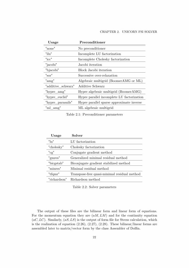
There is multiple choice for solving the LSE Ax = b in FEniCS [1] as illustrated intables 2.1 and 2.2.

In this work, we used the combination (amg, gmres) for solving both the mo-mentum equation and the pressure equation.

2.4 Realization of Unicorn FSI Solver

2.4.1 Converting variational forms to LSE

Form files are files written in Unified Form Language (UFL) embedded in Python.These files specify variational forms of finite element discretizations of differentialequations.

For example in Unicorn, Appendix A.1 shows the form file of the discretizedmomentum equation (2.58). For more form files, we refer to Unicorn source code.

21


Usage Preconditioner

"none" No preconditioner"ilu" Incomplete LU factorization"icc" Incomplete Cholesky factorization"jacobi" Jacobi iteration"bjacobi" Block Jacobi iteration"sor" Successive over-relaxation"amg" Algebraic multigrid (BoomerAMG or ML)"additive_schwarz" Additive Schwarz"hypre_amg" Hypre algebraic multigrid (BoomerAMG)"hypre_euclid" Hypre parallel incomplete LU factorization"hypre_parasails" Hypre parallel sparse approximate inverse"ml_amg" ML algebraic multigrid

Table 2.1: Preconditioner parameters

Usage Solver

"lu" LU factorization"cholesky" Cholesky factorization"cg" Conjugate gradient method"gmres" Generalized minimal residual method"bicgstab" Biconjugate gradient stabilized method"minres" Minimal residual method"tfqmr" Transpose-free quasi-minimal residual method"richardson" Richardson method

Table 2.2: Solver parameters

The output of these files are the bilinear form and linear form of equations.For the momentum equation they are (aM,LM) and for the continuity equation(aC,LC). Similarly, (aS, LS) is the output of form file for Stress calculation, whichis the realization of equation (2.26), (2.27), (2.28). These bilinear/linear forms areassembled later to matrix/vector form by the class Assembler of Dolfin.

22

2.4. REALIZATION OF UNICORN FSI SOLVER

2.4.2 Algorithm of Unicorn FSI SolverThe results of evaluating form files are saved in bilinear and linear forms, for exampleaC,LC for the continuity equation. Assembling these forms in each time step givesthe corresponding matrices and vectors of the LSE problems. For instance, thematrix PM and the vector Pb in the LSE PM∆P = Pb for the continuity equation,where ∆P is the unknown vector.

The general algorithm for solving the FSI system is demonstrated in algorithm1.

23


Algorithm 1 Algorithm of Unicorn FSI Solverfunction initializeVariablesfunction createBilinearLinearFormswhile t ≤ T do . T is final simulation time

function preparestepW0 ←W . mesh velocityX0 ← X . node positionρ0 ← ρ . general density of continuumσ0 ← σ . stress tensorσ0 ← σ . time derivative of stress tensorU0 ← U . velocity - solutionfunction smoothMesh

function stepfor i = 1→ maxit do

function prepareIterationXinc ← k(U+W0)

2 +X0function deform_solidX ← <current position of mesh>W ← X−X0

kP0 ← Pfunction computeStabilization return (d1, d2)function computeP

PM ← assemble(aC)Pb← assemble(LC)function BCs.apply . BCs for pressure eq.∆P ← solve(PM,∆P, Pb)P ← P0 + ∆P

function computeSσ ← assemble(LS)σ ← 1

2(σ + σ0) ∗ k + σ0

function iterJ ← assemble(aM)dotx← assemble(LM)function BCs.apply . BCs for momentum eq.U ← solve(J, U, dotx)

function save(U,t) . save solutiont← t+ k . k is time step, t is current simulation time

24

Chapter 3

Optimization and Testing of theUnicorn FSI solver

3.1 Optimizations

In this work we aim to make the solver more general and robust.In the current Unicorn FSI solver the density was set to unity (ρ ≡ 1), which

limits the solver to cover only certain cases, but not for instance our industrialproblem. Furthermore, there were no previous problems where the force term wasused, meaning that the force was set to zero (f = 0). Moreover, the solver was notwell-tested, in particular a scaling problem was identified in stabilization coefficientsδ1, δ2.

In this chapter we outline the optimizations and tests made to the solver.

3.1.1 Modification of the momentum form file

As discussed in Section 2.3.4, we implemented the formula (2.58) in the Unicorn FSIsolver. The basic improvement is the change to a general density ρ in the form file.and adding stabilization terms for consistency. For details, we refer to AppendixA.1.

The new formula reads:

0 =(ρU , v) + (ρU · ∇U, v) + (ΣD − PI,∇v)− (f, v)+ (ρU · ∇U, δ1ρU · ∇v) + (∇P, δ1ρU · ∇v)− (f, δ1ρU · ∇v) + (∇ · U, δ2∇ · v)

(2.58)to be compared to the old simplified version in the Unicorn FSI solver:

0 =(ρ(U + U ·∇U)− f, v) + (ΣD − PI,∇v)+ (ρU · ∇U, δ1ρU · ∇v) + (∇ · U, δ2∇ · v)

(3.1)

25

CHAPTER 3. OPTIMIZATION AND TESTING OF THE UNICORN FSI SOLVER

3.1.2 Modification of the continuity form file

For the continuity form file, we added the force term and the density term togetherwith corresponding stabilization terms as in the equation (2.56). Details of theimplementation are in Appendix A.2.

New formula:

(∇P, δ1∇q) = −(∇ · U, q)− (ρU · ∇U, δ1∇q) + (f, δ1∇q) (2.56)

The old simplified formula in Unicorn FSI:

(∇P, δ1∇q) =− (∇ · U, q)− (U · ∇U, δ1∇q) (3.2)

3.1.3 Calculating stabilization coefficients

To understand the scaling of the stabilization coefficients δ1, δ2, we here provide adimensional argument.

Set u = Uu∗, x = Lx∗, t = Tt∗, ρ = Φρ∗, p = Pp∗, f = Ff∗

and ∇ = 1L∇

∗, ddt = 1T

ddt∗ , T = L

U , P = ΦU2,where the star ∗ denotes the non-dimensional quantities (scales) and the capitalletters denote the unit.

From the UC system of equations:

∇ · u = 0 Continuity equationρ(u+ u ·∇u) +∇P − µv∆u = f Momentum equation

(3.3)

we rewrite the momentum equation in dimensionless form:

ΦUTρ∗(du

∗

dt∗+ u∗ · ∇∗u∗) + P

L∇∗P ∗ − µv

U

L2 ∆∗u∗ = Ff∗

ΦU2

L

(ρ∗(du

∗

dt∗+ u∗ · ∇∗u∗) +∇∗p∗

)− µv

U

L2 ∆∗u∗ = Ff∗ (3.4)

The Reynold number is defined as Re = ULν = ΦUL

µvwith ν = µv

ρ , so that:

(ρ∗(du

∗

dt∗+ u∗ · ∇∗u∗) +∇∗p∗

)−Re−1∆∗u∗ = f∗ (3.5)

This is so called the non-dimensional momentum-equation.We also rewrite the continuity equation as:

0 = ∇ · u = U

L(∇∗ · u∗) (3.6)

26

3.1. OPTIMIZATIONS

Calculating δ1

We add a stabilization term with parameter δ1 to the momentum equation (3.4),which in variational form can be stated as

(δ1(ρu · ∇u+∇P − f), ρu · ∇v) (3.7)

We study the term inside the integral:

δ1ΦU2

L

ΦUL

(ρ∗u∗ · ∇∗u∗ +∇∗p∗ − f∗) · (ρ∗u∗ · ∇∗v) (3.8)

The terms (3.4) and (3.8) should have the same dimension (unit), such that:

δ1ΦU2

L

ΦUL∼ ΦU2

L

δ1 ∼L

ΦU

(3.9)

where we letδ1 ≡ C1

h

ρu.

In the implementation, we account also for the time-dependent part and theALE description for the convective velocity. Therefore, δ1 contains also informationof the time step k and the ALE velocity.

δ1 = C10.5

ρ

√(1k

)2+(U−Wh

)2 (3.10)

where W is the mesh velocity. The factor 0.5 comes from a theoretical result ofpure transport equations, which states that δ = 1

2hU is the optimal choice [14].

We also add a stabilization term with δ1 to the pressure equation (3.6):

(δ1(ρu · u+∇P − f),∇q) (3.11)

So that the scaling of the integral is:

δ1ΦU2

L

1L

(ρ∗u∗ · u∗ +∇∗p∗ − f∗) · (∇∗q) (3.12)

The terms in (3.6) and (3.12) should also have the same dimension:

δ1ΦU2

L

1L∼ U

L

δ1 ∼L

ΦU

(3.13)

which gives the same result as in (3.9).

27


Calculating δ2

The stabilization term with parameter δ2 is

(δ2(∇ · u),∇ · v), (3.14)

For which the scaling of the integral is:

δ2U

L2 (∇∗ · u∗) · (∇∗ · v) (3.15)

Analogously, the terms (3.4) and (3.15) should have the same dimension:

δ2U

L2 ∼ΦU2

Lδ2 ∼ LUΦ

where we letδ2 = C2ρUh (3.16)

The stabilization terms δ1, δ2 have been modified in Unicorn FSI solver to havethe correct scaling.

3.1.4 Check-point restart

At some point of a simulation, users may want to save the state of a simulation (withall necessary data) so that he/she can use that point as initial values for anothersimulations or simply restart/continue from that point. This feature is implementedin FEniCS solvers, in particular in the Unicorn FSI solver. FSI checkpoint-restartis tested and modified in this project. The result after restarting from a checkpointis exactly same as the result saved during checkpointing.

3.2 New Features

3.2.1 Tracking points

When running a FSI simulation, users can choose one or several interesting solidpoints (vertices) to track its/their coordinates. The coordinates of these pointschange during the simulation as the solid moves but the indices of these pointsremain the same. The idea is based on using the indices to track the points.

• In the initial mesh, we identify the index of an interesting point geometrically,within some defined tolerance. More precisely, we search for a vertex withinthe neighbourhood of a spatial point, which is the measured initial positionof the interesting point, the radius of the neighbourhood is a user-definedtolerance.

28

3.3. TESTING

• If a vertex is found, we store the index of it. This vertex represents theinteresting point.

• Based on this index, we track and print out the changing coordinates of thisvertex.

If there is no vertex found inside the neighbourhood-sphere, the index returned is-1. If there are more than one vertices found in the sphere, the index of nearestvertex to the sphere center is returned.

The implementation of the TrackingPoint class is described in Appendix B.1.

3.2.2 Applying force bases on vertices

Since the solid body moves during the FSI process, the area where the force isapplied on the solid body also moves. The requirement is to move the force alongwith the solid part that the force is applied on.

In Unicorn, the force-area is defined by the part of the mesh that contains thesolid. In form files, force is multiplied with (1 − θ) to identify the solid part. Thisapproach does not describe the right area of the force from the beginning and cancauses possible bugs when one wants to use the force apart from the form files.

We have changed the code to detect vertices in the initial force-area, so calledforce-vertices, to apply the force on. Those force-vertices are saved to TrackingPointobjects. All those objects are stored to the attribute forceV ertices. When the solidmoves, the force-vertices also move. Based on the force-vertices, we apply the forceon them and their neighborhood.

Array < TrackingPoint∗ > forceV ertices;We refer to the source code of the ForceArea class in Appendix B.2 for details.

3.3 Testing

3.3.1 Test problem

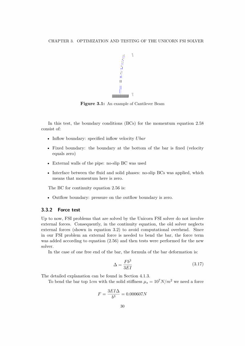
For testing purposes, we used a simple FSI problem: a cantilever beam, shown inFig. 3.1. We used the geometry described in Sec. 1.3. However, we removed thefour pins around the top of the bar, meaning that the steel bar (density 8000kg/m3)now is free to move at one end and is fixed in the other end. The bar is surroundedby flowing water (density 1000kg/m3) or air (in this test air density is assumed tobe 1.0kg/m3) with the inflow velocity Ubar = 1m/s. A force F is applied on thebar as a load in order to bend the top of the bar 1cm in horizontal direction. Whenthe top of the bar reaches the desired bending position, the force is removed andthe bar is released to freely vibrate.

29


Figure 3.1: An example of Cantilever Beam

In this test, the boundary conditions (BCs) for the momentum equation 2.58consist of:

• Inflow boundary: specified inflow velocity Ubar

• Fixed boundary: the boundary at the bottom of the bar is fixed (velocityequals zero)

• External walls of the pipe: no-slip BC was used

• Interface between the fluid and solid phases: no-slip BCs was applied, whichmeans that momentum here is zero.

The BC for continuity equation 2.56 is:

• Outflow boundary: pressure on the outflow boundary is zero.

3.3.2 Force testUp to now, FSI problems that are solved by the Unicorn FSI solver do not involveexternal forces. Consequently, in the continuity equation, the old solver neglectsexternal forces (shown in equation 3.2) to avoid computational overhead. Sincein our FSI problem an external force is needed to bend the bar, the force termwas added according to equation (2.56) and then tests were performed for the newsolver.

In the case of one free end of the bar, the formula of the bar deformation is:

∆ = Fb3

3EI(3.17)

The detailed explanation can be found in Section 4.1.3.To bend the bar top 1cm with the solid stiffness µs = 107N/m2 we need a force

F = 3EI∆b3

= 0.000607N

30

3.3. TESTING

Converting to force density, we have f = F/V = 2.53N/m3. The force is appliedin the y-direction. i.e. normal to the wider surface of the bar. In addition, air flowwith air viscosity was used.

As can be seen in Fig. 3.2, the y-coordinate change of the bar top reached themaximum ≈ 10mm.

Figure 3.2: Coordinate change of the bar top during the bending process under the forcedensity f = 2.5N/m3.

The result of the pressure inside the pipe under an external force is plotted inFig. 3.3. A difference in pressure in the direction of movement of the bar is observed,which shows that the solver works according to corresponding physics phenomena.

(a) (b) (c)Figure 3.3: Pressure inside the air channel under a bending force by the new FSI solver;(a) Overview: a slide cut through the channel in the y-direction; (b) A zoomed-in slide cuton the bar top in the y-direction; (c) A zoomed-in slide cut on the bar top in the x-direction;

3.3.3 Velocity and Pressure comparison

Using both the old FSI solver and the new solver to run the same combination ofparameters, we compare the results. In the remaining test cases of chapter 3.3, noexternal force was applied.

31


In order to have a rough approximation of the flow velocity inside the pipe, wemake a calculation based on the relation of flow velocity and cross sectional-areaof the pipe. The flow is accelerated inside the pipe as there is narrower flow crosssection (because of the bar). We calculate the velocity of the flow in the channelwhere the bar is:

• At the inflow: the cross sectional-area of the flow is S1 = 80mm × 80mm =6400mm2 with the mean velocity Ubar = 1m/s.

• At the slide cut in the middle of the bar: The cross sectional-area of thebar: 8mm × 20mm = 160mm2. The cross sectional-area of the flow is S2 =6400mm2 − 160mm2 = 6240mm2, which implies that the mean velocity isU2 = Ubar×S1

S2= 1.026m/s.

Comparing the two cases (a) and (b) in Fig. 3.4 for the air flow case (which isassumed to be incompressible as discussed in Sec. 2.2), we observe that the resultingvelocity U of the old solver is higher than the one in the new solver. According tothe calculation above, the result from the new solver seems to be more reasonablesince it is closer to the value 1.026m/s.

The old solver does not handle the case of water flow (as well as other flowmaterial with density different from unity), whereas the new solver can. For instancethe new solver can handle the water flow (density 1000kg/m3), the result shown inFig. 3.4(c). In this water flow case, the velocity field has lower values comparedto the air flow case, which can be explained by the effect of higher viscosity: waterviscosity is about 90 times larger than air viscosity, which lead to the fact thatwater resists the tendency of the flow more than air.

The pressure plots shown in Fig. 3.4 are the pressure difference between a pointinside the pipe and the outflow surface (where we assume a zero pressure). Thepressure of the water flow is higher than the pressure of the air flow, which can beexplained by higher density of water: a larger number of molecules in a volume unitcreates a higher pressure.

32

3.3. TESTING

(a) (b) (c)Figure 3.4: Velocity U(m/s) and Pressure P (Pa) for the cantilever problem with theinflow velocity 1m/s; (a) The old FSI solver for air flow (ρ ≡ 1kg/m3); (b) The new FSIsolver for air flow (ρf = 1kg/m3; ρs = 8000kg/m3); (c) The new FSI solver for water flow(ρf = 1000kg/m3; ρs = 8000kg/m3).

3.3.4 Test the FSI-solver as an Incompressible Navier-Stoke solver

The idea here is that if the solid part is removed from the problem, the FSI-solver0

should be able to handle the turbulent flow case as the pure fluid Unicorn solvercalled Incompressible Navier-Stoke solver (ICNS-solver) [1] does. In this test case,the bar is removed from the pipe but the bottom cross (shown in Fig. 1.1(c)) isremained; water or air is pumped into the pipe with an inflow velocity 1m/s.

Fig. 3.5(a) illustrates the results of the FSI solver for water flow. The solver isstable for this case since it ran over all simulation time T = 5s. As can be seen, theflow is stable and turbulence appears in the downstream behind the cross, whichindicates that the FSI solver can handle turbulent flow simulations.

Fig. 3.5(b)(c) show that for air flow case the results of the FSI-solver in (b) aredifferent compared to the results from the ICNS-solver in (c). The FSI solver givesa lower velocity than the one from the ICNS solver. The velocity is accelerated dueto the incompressibility assumption in both solvers and the cross on the bottom of

0From now the FSI solver is referred to as the new FSI solver.

33


the geometry. To identify which result is more realistic, we propose to measure alsothe velocity and the pressure in the real experiments.

(a.1) (a.2) (a.3)

(b.1) (b.2) (b.3)

(c.1) (c.2) (c.3)Figure 3.5: (a) Turbulent water flow by the new FSI-solver; (b) Turbulent air flow bythe new FSI-solver; (c) Turbulent air flow by the ICNS-solver; (1) The pressure throughthe pipe; (2) Overview of a velocity slide-cut along the pipe; (3) Zoomed-in to the bottomcross part of the velocity slide-cut (2);

3.3.5 Sensitivity with respect to physical parameters

In each test case below only the test input parameter was changed and the rest inputparameters were fixed. The main subject to be studied here is how the change of

34

3.3. TESTING

input parameters influences the output infinity norm of the velocity vector field.If variation of the velocity magnitude becomes smaller than a threshold over time,we say that the solution converts and stability is established. In contrast, if thevelocity magnitude reaches to infinity (or a large number) we call that the solutiondiverts and the solver is unstable.

Solid stiffness µsOne of the interesting parameters that may affect the sensitivity of the solver isthe solid stiffness (Young’s modulus). Fig. 3.6 illustrates the infinitive norm of thevelocity magnitude over time.

(a) (b) (c)Figure 3.6: Sensitivity of the FSI solver with respect to solid stiffness: (a) With fluid:soliddensity 1:1 (air density); (b) With fluid:solid density = 1:8000 (air/steel densities); (c) Withflui:solid density = 1000:8000 (water/steel densities);

We compared three Young’s modulus of the bar: the stiffness of paper E =1e3N/m2, the stiffness of rubber E = 1e7N/m2 and the stiffness of steel E =19e9N/m2. These three Young’s modulus were tested with three different combi-nations of fluid/solid densities.

As can be seen in Fig. 3.6 the results with respect to different stiffness are quitesimilar. However, in the case (c) the stiffness of paper appears to be easier for thesolver to handle. In conclusion, in cases without the external force and low fluiddensity, the sensitivity of the solver appears not to depend on the stiffness of thesolid material. In contrast, for high fluid density the lower the stiffness, the higherstability of the solver.

Density ρ

For the density test, two cases are studied:

1. Scaling of density: we use the same density for both fluid and solid, and scalethat common density;

2. Density difference: we use different density for fluid and solid.

35


In these two test cases, the solid stiffness was set to E = 1e7N/m2 and the fluidviscosity to µv = 0.00001983Ns/m2.

In the first test case we changed the density for both phases from 1 to 10,100, 1000 and 2000kg/m3. The results are demonstrated in Fig. 3.7. As canbe seen, scaling the density from 1 to 1000kg/m3 causes the velocity to be moreunstable in the beginning of the simulations. The larger the scale, the broader thevelocity variation and the later the velocity gets to its steady state. However, for thedensity 2000kg/m3 the velocity diverted. Consequently, larger density scale makesthe solver become more sensitive.

Figure 3.7: Density scaling: Fluid:solid density scaled from 1:1 to 2000:2000 (kg/m3)

The second test case studies the sensitivity of the FSI solver concerning thedifference in density of the two phases. Fig. 3.8 show the infinitive norm of thevelocity magnitude during simulation time. As shown, both increasing the fluid orsolid density causes the solver to be more unstable. Comparing the cases 1:8000and 100 : 8000: the bigger difference in density is more stable. While comparing thecases 1000 : 8000 and 1000 : 2000, the bigger difference in density is more unstable.It can be concluded that the more/or less difference in density does not seem toplay an important role in the solver’s sensitivity.

36

3.3. TESTING

Figure 3.8: Difference in density: Fluid:solid densities changed from 1:8000 to 1000:8000,1000:2000 (kg/m3)

Fluid viscosity µv

In this section the effect of the fluid viscosity is studied.As can be seen in Fig. 3.9 a higher viscosity of the fluid (water viscosity versus

air viscosity) does not seem to improve the stability of the solver. However, an"artificial" viscosity can stabilize the solver. "Artificial" viscosity means that we setthe viscosity of the fluid as a function that can stabilize the velocity, so that

µv := µv + ρh ||U || (3.18)

where h is the local cell size and U is the local velocity in the cell.On the other hand, as the fluid viscosity has a big influence on the movement

of the solid, for accuracy it is not recommended to increase the fluid viscosity forthe solver stabilization.

37


Figure 3.9: Viscosity compare: water dynamic viscosity µv = 0.00136857Ns/m2; airdynamic viscosity µv = 0.00001983Ns/m2; and "artificial" viscosity µv := µv +ρh ||U || withµv = 0.00136857Ns/m2.

3.3.6 Sensitivity with respect to simulation parameters

Time step k

The solver stability depends strongly on time step k. Taking large time steps cansave computational cost and make the simulation faster. On the other hand, itmeans that numerical results contain larger discretization error, or even worse -large time steps can make results unstable and whole simulation crash. Therefore,the size of time step should be inside a limit, for instance in the FSI solver the CFLcondition is used. The CFL condition states that the time step must be less thanthe time for a wave to travel across one mesh cell (k < h/U), then the algorithmis CFL stable. Nevertheless, small time steps guarantee more stable run but theyrise the computational cost and make the simulation more slow. In addition, toosmall time step can also affect other quantities, which depend on the time steps, forexample the stabilization coefficient d1 in equation (3.10).

Fig. 3.10 shows that a larger time step (which is inside a CFL limit) can bemore stable than small time steps. The reason is the stabilization coefficient d1depends on time steps k. When k is too small, the term 1/k2 will dominate theterm (U −W )2/h2 and defect the effect of d1-stabilization. One suggestion is tomodify the stabilization coefficient d1 so that the terms 1/k2 and (U −W )2/h2 arein the same order.

38

3.3. TESTING

Figure 3.10: Velocity magnitude result of the solver with different time steps. Thetime steps depend on the minimum cell size, the inflow velocity and a CFL constant: k =CFL ∗ hmin/Ubar

Stabilization coefficients C1, C2

We study the scaling of the stabilization coefficients C1, C2 mentioned in equations(3.10) and (3.16).

Scaling up the stabilization coefficients can help to stabilize the solver. Theplots in Fig. 3.11 illustrate the less sensitive results by scaling up the stabilizationcoefficients by a factor of 2. However, increasing stabilization coefficients meansthat we allow a higher perturbation of the system, which leads to the fact that theoutput velocity is more stable but it can converge to a number that further awayfrom the realistic velocity.

39


Figure 3.11: Scaling up the stabilization coefficients by a factor of 2

40

Chapter 4

Application of the Unicorn FSI Solver

We use the FSI solver to simulate the target problem mentioned in chapter 1. Wemention here tasks that need to be performed as an user of the FSI solver.

4.1 Simulation preliminaries

4.1.1 Mesh generation

Software ANSA [15] is used in this step.Firstly, we read CAD input data into ANSA and cleaned up the geometry.

After that, surface meshing and volume meshing were done with the help of ANSABatch Manager. Meshes from ANSA is exported to NAS format, then GMSH [16]converted .nas to .msh. After all, dolfin-convert is used to convert .msh to .xml.The final .xml mesh is the input of the solver.

We exported here two meshes: the whole domain mesh and bar mesh (solidmesh).

Properties Solid mesh Whole mesh

Number of vertices 18004 170999Number of cells 71571 918062Range of cell size 0.8 - 1.0 mm 0.8 - 5.0 mm

Table 4.1: Mesh properties

41

CHAPTER 4. APPLICATION OF THE UNICORN FSI SOLVER

4.1.2 Parameters

Parameter Notation Value Unit

solid stiffness µs 193e9 (steel); 1e7 (rubber) N/m2

solid density ρs 8000 (steel); 1100 (rubber) kg/m3

fluid viscosity ν * Table 4.3 m2/s

fluid density ρf 1000 (water); 1 (air) kg/m3

fluid inflow Ubar 1 m/s

simulation time T * 5.0 s

time step k * 0.01hmin/Ubar s

external volume force f * 2.5 N/m3

number of samples N * 200 -* Adjustable by user

Table 4.2: Parameter list

TemperatureoC

Water dynamic viscosity(kg/ms)× 10−3

TemperatureoC

Air dynamic viscosity(kg/ms)× 10−5

7.4 1.41 15 1.8648.4 1.36857 27 1.98310 1.30627

11.7 1.2449715 1.13857

Table 4.3: Water and air viscosity

The Reynolds number is defined by Re = ρuLµv

= uLν . For this problem, we take

L = 30mm, the minimum distance from bar to pipe wall; u = 1m/s is the same asthe inflow velocity. The Reynolds number is:

Re = 1m/s ∗ 30× 10−3m

1.41× 10−6m2/s≈ 22× 104

4.1.3 Bending forceForce for Beam with contact problem

This problem is similar to the case Beam fixed at one end and supported (pined) atthe other end in Fig. 4.1. The bending force used in this case is concentrated force

42

4.1. SIMULATION PRELIMINARIES

at the middle point of the bar.

Figure 4.1: Beam with contact problem (supported pin)

Denote:F is the concentrated force at point Ca = 0.75m - distance from C to free end of the beamb = 0.75m - distance from C to fixed end of the beamL = 1.5m - the length of the beamB = 20mm = 0.02m - the width of the beamH = 8mm = 0.008m - the thickness of the beam∆ = 10mm = 0.01m - deformationE = µs = 193e9N/m2 the Young modulus/stiffness of steelI = BH3

12 = 853e− 12m4 Inertial momentum

According to [17] we have formula:

∆ = Fa2b3

12EIL3 (3L+ a) (4.1)

To bend the bar to the maximum amplitude ∆ = 10mm away from the initialposition, an external force F = 53.53N needed to be applied in the middle area ofthe bar. We measure the distance between mid-bar point and the center. Whenthis distance reaches to 10mm, we stop the external force.

Depending on the implementation of solver Unicorn, we convert the bendingforce F in N to force density f = F/V in N/m3. Where V is the volume (force-area), on which force is applied.

Physically, force should be applied in the middle of bar within a small thickness1mm, then V ≈ 16e−8m3 and f ≈ 335e6N/m3. Due to the instability of the solverif f is too large, we make f smaller by considering that concentrated force can beconverted into load force on whole bar. Then we make force-area be the wholebar and V = BarV olume = 1.5 × 0.02 × 0.008 = 24 ∗ 10−5m3 and consequentlyf = F/V = 223100N/m3.

43


Force for cantilever beam

For a cantilever beam, the formula for deformation is:

∆ = Fb3

3EI(4.2)

To bend the bar top 1cm with the solid stiffness µs = 107N/m2 we need a force

F = 3EI∆b3

= 0.000607N

Converting to force density, we have

f = F/V = 2.53N/m3. (4.3)

Smoothly increasing force

In consideration of avoiding shock that can be created by the force, we introducethe force as a smooth-step function by multiplying f with a function ramp(t). Con-sequently, the force increases from zero to f .

ramp(t) =

0 t in [0, t1]6t5t − 15t4t + 10t3t t in (t1, t2], tt = t−t1

t2−t1 in (0, 1]1 t in (t2, T ]

(4.4)

The force should increase gradually, so that the bar will not accelerate too much.Ideally, during the bending movement, the bar should always be in the equilibriumof the bending force and its internal stress force.

4.2 Implementation preliminaries

4.2.1 Tracking pointsIn order to measure the frequency and the amplitude of the vibrating bar, we keeptrack of a point, which characterizes the vibration. For instance, in the cantilevercase this point is a point on the top of the bar. In the case of a pinned bar, theinteresting point lays in the middle of the bar. The tracked point has approximatelythe maximum amplitude in comparison to other points of the bar and can describethe interesting quantities the best. During a simulation, the coordinates of thistracked point are printed out in each time step.

4.2.2 Checking the end of the bending processIn order to check if the bar has reached to the desired bended position (1cm awayfrom the initial position), we have two checks:

44

4.3. RESULTS

• A vibrating point is tracked as described above. In each time step, we checkthe distance of the current position of this point to the initial coordinates ofit. If this distance is larger than 1cm, we flag that "the bar has bended".

• Another check is when the force function has reached to its maximal value.However, when the force has reached to its maximal value, the bar may stillbe on the way to its maximum bended position. Therefore, the force shouldbe maintained for a while until the bar has reached the equilibrium positionwith this force and stops moving.

4.2.3 Boundary Conditions

Boundary conditions for momentum equation consist of:

• Inflow boundary: Specified inflow velocity Ubar

• Fixed boundary: Boundary on the bottom of the bar should be fixed (mo-mentum equals zero)

• External wall of the pipe: no-slip BC

• Interface between the solid and the fluid: We applied here no-slip boundary,which means momentum is zero.

Boundary condition for continuity equation is:

• Outflow boundary: pressure in outflow boundary is zero.

4.3 Results

In this section we introduce test results of the geometry described in Section 3.3.The bar is made from rubber (stiffness 1e7kg/ms) and was bended and releasedin an air flow (inflow velocity 1m/s) with fluid density 1kg/m3. We also used theunity density for the solid part as it is a stable setting. The simulations were carriedout with two different fluid viscosities.

In the simulation, first the bar is bended by an external force (the bendingprocess) until the top of it reached nearly 1cm in the y-direction. Then the barwas released (the force was removed) and freely vibrated. All of these processeswere simulated by the FSI-solver. The obtained results from the FSI-solver of thevibrating rubber bar give a good condition for simulating the vibration of a steelbar as in the real experiments. It also indicates that the new FSI-solver is able tosimulate a real industrial FSI problem.

45


4.3.1 Simulation with high viscosity of the fluid

The first result that we will analyse is the case of high fluid viscosity. As known,viscosity represents the "resistance" of the fluid to movements, in particular themovement of the bar that immersed into it. A higher viscosity implies a largerresistance.

In this test case we set the "artificial" viscosity to the fluid as in (3.18). Fig. 4.2illustrates the region of the mesh around the top of the bar. The bar region is the"blue straight" region.

(a) (b) (c)Figure 4.2: A slide cut on the top of the bar (a) in the initial position, (b) in bended(extreme) position and (c) when it was coming back to the initial position

In Fig. 4.2(a), the bar is in its initial position. Then an external force is appliedon the bar to bend it (to the right as seen in Fig. 4.2). During the movement ofthe bar, most of the fluid elements around the bar are deformed: they are stretchedin one side of the bar and are squeezed in the other side. The deformation of theelements may result in bad quality of them (flat elements with small angels), whichcause the FEM stiffness matrix to be ill-conditioned [18]. To avoid this problem,the Elastic Smoother of the FEniCS is used to smooth the mesh and improve thequality of the elements in each time step. The images in Fig. 4.2 show the smoothedelements by the Elastic smoother.

Fig. 4.2(b) shows the top of the bar when it reached to the equilibrium position,meaning that the internal stress force equals the external force (volume force f =2.5N/m3). As shown in Fig. 4.3, the bar has not reached 1cm in the y-direction ascalculated by equation (4.3). This result may be explained by the high viscosity ofthe fluid.

Next, the force is removed. Due to the internal stress force, the bar is movingback toward its initial position, which is shown in Fig. 4.2(c).

46

4.3. RESULTS

Figure 4.3: Coordinate changes of the top of a rubber bar during bending and vibrationprocesses with fluid viscosity µv := µv + ρhU

Fig. 4.3 illustrates the coordinates of one point on the top of the bar duringthe whole process described above. Note that since the force was applied in they-direction, we are more interested in the y-coordinate of the point. As can be seen,when moving toward the initial position after being released, the bar did not crossthe initial position to move further to another side (no vibration). Indeed, it wasreaching to the initial position and the movement was damped quickly. The curveof the movement is similar to the one of a critical damping situation. As mentioned,this situation relates to the high viscosity of the fluid, which resists and damps outthe movement of the bar.

4.3.2 Simulation with air viscosity of the fluidIn contrast to the result of the high viscosity above, in this test case we used theviscosity of air and the initial condition of the bar is in its bended position. Twosnapshots of the bar movement are demonstrated in Fig. 4.4.

(a) (b)Figure 4.4: A slide cut on the top of the bar: (a) in bended (extreme) position at t = 0.4sand (b) during the vibration

47


In Fig. 4.4(a), the bar is in its bended position. No force is applied on thebar from this moment. Thereafter, the bar is moving toward its initial positionand crosses this position. Further, the bar moves to the other side and reachesto a maximum amplitude of 4.2mm. Fig. 4.4(b) shows the position of the bar atthis moment. Then, the bar keeps vibrating with a damping effect, which will beanalysed below.

The coordinates changes of one point on the top of the bar are shown in Fig. 4.5.In this figure we also show the coordinates of the bar during the bending process(from t = 0 to t = 0.4s) for a better detection of the initial position.

Figure 4.5: Coordinate changes of the top of a rubber bar during bending and vibrationprocesses in an air flow

Based on the observation of the amplitude in Fig. 4.5, the period of oneoscillation in the y-direction is T = 0.8s, the vibration frequency calculated isf = 1/T = 1.25Hz. Using the formula of the damping ratio from solid mechanics,for instance in [19], it holds that:

ln(x1x2

)= 2πδm√

1− δ2(4.5)

where:x1 is the amplitude of the first oscillation at time t,x2 is the amplitude of the oscillation that occurs ’m’ cycles later (occurs mT secondlater),δ is the damping ratio.

It can be measured that x1 = 9.2mm; x2 = 1.9mm for m = 1. Applying theequation (4.5) we calculated the damping ratio of this oscillation:

δ = 0.2435

This is the under-damped oscillation (δ < 1), in which the amplitude generallyreaches its zero position while oscillating around this zero.

48

4.3. RESULTS

In conclusion, the external bending force can mimic the real physical force in thisproblem. The simulation results reflect the physical rules of viscosity. Furthermore,the vibration of the rubber bar convinces that the new FSI-solver is able to handlethis industrial problem.

49

Chapter 5

Discussion and Future work

5.1 Summary

The problem setting, simulation preliminaries and parameters preparation are donefor the target FSI problem. The user interface code is rearranged into functionsand classes with comments, some new features are implemented, which providemore ease for future users to work with the FSI solver.

The generality to choose density is successfully implemented in the FSI solver,which makes both the resulting velocity and pressure closer to realistic values.

The force term is included in the mathematical model, implemented and testedfor the cantilever problem. The test result is reasonable.

Parameter studies were performed to test the sensitivity of the FSI solver. Look-ing at the test results we can see the influence of different aspects to the stabilityof the solver.

Some testing results were obtained, which promise a future success for simulatingthe real experiments.

5.2 Future improvements of the FSI solver

The tests in Section 3.3 show that there are still numerical instability problems inthe new FSI solver. The sources of this problem may come from different aspects:the applied UC mathematical model, possible bug(s) in the implementation, meshquality issues, insufficient combination of physical and simulation parameters.

On the external wall, at the moment there is only one working choice for bound-ary condition (no-slip), which lower the physical reality of the simulation. Theslip-boundary condition choice is implemented but not well-tested. Future workshould include the testing performance of the slip BC.

51

CHAPTER 5. DISCUSSION AND FUTURE WORK

5.3 Contact Modelling

5.3.1 A Simplified modelThe discussed experiment in Section 1.3 has a contact problem (contact betweenthe balls on the cylinder tips and the top of the bar). Solving this contact problemdemands more analysis and workload (one solving method is mentioned in Section5.3.2). To make the simulation easier, we first suggest to simplify this problem asdescribed below.

We choose one point (vertex), where the intersection of the four cylinders is (seeFig. 1.1). This point is an inner point laying inside the top of the bar. The pointwill be fixed from sides (fix in horizontal x- and y-directions) and be free to slide upand down (free in vertical z-direction). The balls on the cylinder tips are removedto leave empty spaces between the cylinders and the bar. Therefore, we simplifythe problem by neglecting the contact problem between the top of the bar and fourcylinders, but we still expect the same effect as four small balls on cylinders create.

Furthermore, the four cylinders are removed to save computational cost, sincethe cylinders do not affect the interesting flow and the bar movement.

Mathematically, we enforce the fixed point by zero out the x- and y-componentof the corresponding vertex in the right-hand-side b of the momentum LSE Ax = b;the z-component is untouched. Hence, during the simulation the result velocity ofthis fixed point in the horizontal x- and y-directions are zero; and in the verticalz-direction is kept. In the implementation, we have created a Mesh function, whichis true in fixed-point-vertex, and false otherwise. To be coupled with this meshfunction, we also pass a vector with a special value (extremely large value that isunreasonable for real physical velocity) for MeshBC class to "recognize" the fixed-point vertex. MeshBC class will enforce zero for x- and y-component of this fixed-point vertex. We refer to Appendices B.3 and B.4 for details.

This simplified model was implemented and tested in the old FSI solver. Un-fortunately, the result was unstable. It could be related to several aspects that hadnot been fixed in the old solver. In future work, we can test this model again withthe new solver after solving the instability problems.

5.3.2 Contact modelIn the contact model we keep the original setting for the mesh (with four cylinders).The ball areas between the four pins and the bar are called four interacting areasand are set to be solid with a special material (defined by user), for instance rubber.In other word, we make the four balls become rubber.

The contact model is implemented in the new FSI solver. The preliminaryresults showed that in the time period under a bending force, the middle point ofthe bar moved much more than the top of the bar (Fig. 5.1), which promises apossible approach for our target problem. However, the question of which contactmaterial should be used plays an important role in this model.

52

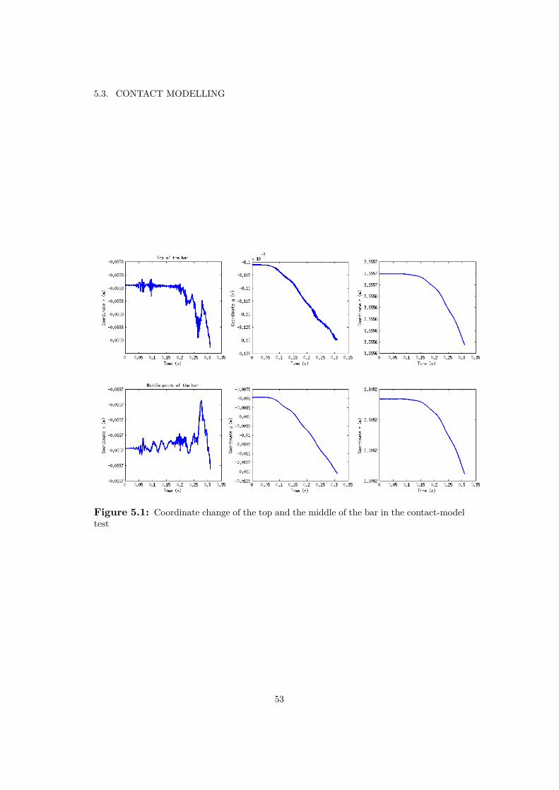
5.3. CONTACT MODELLING

Figure 5.1: Coordinate change of the top and the middle of the bar in the contact-modeltest

53

Bibliography

[1] FEniCS team. FEniCS project. http://fenicsproject.org, 2003. [Online;Accessed: 2013-09-30].

[2] Stuart J. Price Michael P. Paidoussis and Emmanuel de Langre. Fluid-StructureInteractions Cross-Flow-Induced Instabilities. Cambridge University Press,2010.

[3] S. Rugonyi and K. J. Bathe. On finite element analysis of fluid flows fullycoupled with structural interactions. Tech Science Press, 2:195–212, 2001.

[4] Michael Stoeckli. A unified continuum fluid-structure interaction solver usingan ALE finite element method. Master thesis, KTH, 2007.

[5] Ren de Borst Erwin Stein and Thomas J.R. Hughes. Encyclopedia of Com-putational Mechanics, volume 1: Fundamentals. John Wiley and Sons, Ltd.,2004.

[6] J. Jansson J. Hoffman and Michael Stockli. Unified continuum modelling of 3dfluid-structure interaction. Preprint KTH-CTL-1003 Computational Technol-ogy Laboratory, 2009.

[7] Johan Hoffman and Claes Johnson. Computational Turbulent IncompressibleFlow: Applied Mathematics Body and Soul Vol 4. Springer, PDF version avail-able at www.csc.kth.se/jhoffman/pub/v4.pdf, 2006.

[8] Richard Fitzpatrick. Fluid Mechanics. The University of Texas at Austin,http://farside.ph.utexas.edu/teaching/336L/Fluidhtml/, 2012. [On-line; Accessed: 2013-04-03].

[9] T. Dunne and R. Rannacher. Adaptive finite element simulation of fluid struc-ture interaction based on an eulerian variational formulation. Springer, pages110–145, 2006.

[10] Ulrich Ruede. Lecture notes for SIWIR-2. FAU Erlangen-Nuremberg, 2012.

[11] P. Hansbo K. Eriksson, D. Estep and C. Johnson. Computational DifferentialEquations. Cambridge Univ. Press, 1996.

55

http://fenicsproject.org

www.csc.kth.se/jhoffman/pub/v4.pdf

http://farside.ph.utexas.edu/teaching/336L/Fluidhtml/

BIBLIOGRAPHY

[12] E. Marchandise G. Compere and J.-F. Remacle. Transient adaptivity appliedto two-phase incompressible flows. pages 1923–1942. Journal of ComputationalPhysics 227, 2008.

[13] John Douglas Faires Richard L. Burden. Numerical Analysis. Brooks/Cole-Thomson Learning, seventh edition, 2001.

[14] Dmitri Kuzmin. A Guide to Numerical Methods for Transport Equations. FAUErlangen-Nuremberg, 2010.

[15] BETA CAE Systems S.A. Ansa - advanced multidisciplinary cae pre-processingtool.

[16] Christophe Geuzaine and Jean-François Remacle. GMESH - A three-dimensional finite element mesh generator. http://geuz.org/gmsh/. [Soft-ware; Accessed 2013-04].

[17] The James F. Lincoln Arc Welding Foundation Adam Sprecace. Beam LoadEquations. http://sprecace.com/node/43. [Accessed 2013-04].

[18] Jonathan Richard Shewchuk. What is a Good Linear Element? Interpo-lation, Conditioning, and Quality Measures. In 11th International MeshingRoundtable, pages 115–126, 2002.

[19] D.J.Dunn. Solid mechanis - Dynamics - Tutorial: Damped vibrations.http://www.freestudy.co.uk/dynamics/damped%20vibrations.pdf. [Ac-cessed 2013-11].

56

http://geuz.org/gmsh/

http://sprecace.com/node/43

http://www.freestudy.co.uk/dynamics/damped%20vibrations.pdf

Appendix A

Form Files Implementation

Listing A.1: NSEMomentum3D.form script:

1 cell = " tetrahedron "23 K1 = VectorElement (" Lagrange ", cell , 1)4 # Dimension of domain5 d = K1. cell_dimension ()6 K2 = FiniteElement (" Lagrange ", cell , 1)7 K3 = FiniteElement (" Discontinuous Lagrange ", cell , 0)8 K4 = VectorElement (" Discontinuous Lagrange ", cell , 0)9 K5 = VectorElement (" Discontinuous Lagrange ", cell , 0, d * d)1011 v = TestFunction (K1)12 U1 = TrialFunction (K1)13 UP = Function (K1)14 U0 = Function (K1)15 Uc = Function (K1)16 Um = Function (K4)1718 P = Function (K2)19 Phydro = Function (K2)20 nu = Function (K3)21 d1 = Function (K3)22 d2 = Function (K3)23 ff = Function (K1)24 fc = Function (K1) # coriolis force25 k = Function (K3)2627 rho_f = Function (K2)28 theta = Function (K3)29 sigma = Function (K5)3031 mu = Function (K3)32 lmbda = Function (K3)3334 WP = Function (K1)

57

APPENDIX A. FORM FILES IMPLEMENTATION

35 Wm = Function (K4)3637 b = Function (K3)3839 rho_s = Function (K3)4041 rho = mult(theta , rho_f) + mult (1.0 - theta , rho_s)424344 def tomatrix (q):45 return [ [q[d * i + j] for i in range(d)] for j in range(d) ]4647 sigmaM = tomatrix (sigma)48 beta = Function (K2) # friction parameter49 tau1 = Function (K)50 tau2 = Function (K)515253 def ugradu (u, v):54 return [dot(u, grad(v[i])) for i in range(d)]5556 def E(e, mu , lmbda):57 Ee = 2.0 * mult(mu , e) + mult(lmbda , mult(trace(e), Identity (d

)))58 return Ee5960 def epsilon (u):61 return 0.5 * (grad(u) + transp (grad(u)))6263 beps = mult(b, epsilon (0.5* Uc))6465 Sf = mult(P, Identity (d)) - mult(nu , grad(Uc))66 Ss = mult(P, Identity (d)) - mult (1.0 , sigmaM ) - beps67 S = mult(theta , Sf) + mult (1.0 - theta , Ss)6869 Uc_ALE = Uc - WP70 Um_ALE = Um - Wm7172 def f(u, v):73 return -dot(mult(rho_f , ugradu (Uc_ALE , Uc)), v) + \74 dot(S, grad(v)) + \75 -mult(d1 , dot(mult(rho_f , ugradu (Um_ALE , Uc)),76 mult(rho_f , ugradu (Um_ALE , v)))) + \77 -mult(d1 , dot(grad(P), mult(rho_f , ugradu (Um_ALE , v)))) +

\78 mult(d1 , dot(mult (1.0 - theta , ff), mult(rho_f , ugradu (

Um_ALE , v)) )) + \79 -mult(d2 , dot(div(u), div(v))) + \80 dot(mult (1.0 - theta , ff), v)8182 def fb(u, v):83 return -beta *( dot(Uc ,tau1)*dot(v,tau1) + dot(Uc ,tau2)*dot(v,

tau2))84

58

85 def dfdu(u, k, v):86 return -dot(mult(rho_f , ugradu (Uc_ALE , u)), v) + \87 -mult (1 - theta , mult(k, dot(E( epsilon (u), mu , lmbda),

grad(v)))) + \88 -mult (1 - theta , mult(b, dot( epsilon (u), grad(v)))) + \89 -dot(mult(theta*nu , grad(u)), grad(v)) + \90 -mult(d1 , dot( mult(rho_f , ugradu (Um_ALE , u)),91 mult(rho_f , ugradu (Um_ALE , v)))) + \92 -mult(d2 , dot(div(u), div(v)))9394 def dfdub(u, k, v):95 return -beta *( dot(u,tau1)*dot(v,tau1) + dot(u,tau2)*dot(v,tau2

))9697 # cG (1)98 def F(u, u0 , k, v):99 uc = mult (0.5 , u + u0)100 return (-dot(mult(rho , u), v) + dot(mult(rho , u0), v) + mult(k

, f(uc , v)))101102 def dFdu(u, u0 , k, v):103 uc = mult (0.5 , u)104 return (-dot(mult(rho , u), v) + mult(k, dfdu(uc , k, v)))105106 def Fb(u, u0 , k, v):107 uc = mult (0.5 , u + u0)108 return (mult(k, fb(u, v)))109110 def dFdub(u, u0 , k, v):111 uc = mult (0.5 , u)112 return mult (1.0 * k, dfdub(uc , k, v))113114 a = (dFdu(U1 , U0 , k, v)) * dx + (dFdub(U1 , U0 , k, v)) * ds115 L = (dFdu(UP , U0 , k, v) - F(UP , U0 , k, v)) * dx + (dFdub(UP , U0 , k

, v)) * ds - Fb(UP , U0 , k, v) * ds

Listing A.2: NSEContinuity3D.form script:

1 cell = " tetrahedron "23 K1 = VectorElement (" Lagrange ", cell , 1)4 # Dimension of domain5 d = K1. cell_dimension ()6 K2 = FiniteElement (" Lagrange ", cell , 1)7 K3 = FiniteElement (" Discontinuous Lagrange ", cell , 0)89 q = TestFunction (K2) # test basis function scalar10 P = TrialFunction (K2) # trial basis function11 P0 = Function (K2) # trial basis function1213 rho = Function (K2)1415 uc = Function (K1) # linearized velocity

59

APPENDIX A. FORM FILES IMPLEMENTATION

16 Wc = Function (K1) # mesh velocity1718 delta1 = Function (K3) # stabilization parameter1920 k = Function (K3)2122 theta = Function (K3)23 f = Function (K1)24 fc = Function (K1)2526 n = FacetNormal (cell)2728 i0 = Index () # index for tensor notation29 i1 = Index () # index for tensor notation3031 def ugradu (u, v):32 return [dot(u, grad(v[i])) for i in range(d)]3334 eps = 0.035 alpha = 2*k36 Uc_ALE = uc - Wc3738 a = (eps*P*q + delta1 *dot(grad(P), grad(q)) + alpha*dot(grad(P),

grad(q)))*dx39 L = (-q*div(uc))*dx + alpha*dot(grad(P0), grad(q))*dx - mult(

delta1 , dot( mult(rho , ugradu (Uc_ALE , uc)), grad(q) ))*dx + \40 delta1 *dot( mult (1.0 - theta , f), grad(q))*dx

60

Appendix B

New Features Implementation

Listing B.1: TrackingPoint.h script:

1 # ifndef __TRACKING_POINT_H2 # define __TRACKING_POINT_H34 # include <dolfin .h>5 namespace dolfin namespace unicorn 67 class TrackingPoint : public SubDomain8 /// Take coordinates of a point , find its index , fix this index

during solving9 10 public :11 // constructor12 TrackingPoint (Point fp , Mesh* inmesh , real tolerance )13 14 this ->tol = tolerance ;15 localMesh = inmesh ;16 // take index of tracked point17 index_fp = checkIndex (fp , localMesh , tol);1819 // take coordinates of fixed_point by its index20 if (this -> index_fp > -1) 21 Vertex v(* localMesh , (uint) index_fp );22 coord = v.x();23 24 else coord = NULL ;25 2627 // take coordinates of point and return index of nearest vertex28 int checkIndex ( const Point p, Mesh* mesh , real tolerance ) const29 30 real min_dist = 100000;31 uint ver_idx ;3233 for ( VertexIterator v(* mesh); !v.end (); ++v)

61

APPENDIX B. NEW FEATURES IMPLEMENTATION

34 Vertex & vertex = *v;35 Point pref = vertex .point ();3637 if (p. distance (pref) < min_dist )38 39 min_dist = p. distance (pref);40 ver_idx = vertex .index ();41 42 43 if ( min_dist < tolerance ) return (int) ver_idx ;44 else return -1;45 4647 real* x() const // return current coordinates of the point48 49 return coord;50 5152 int* index () const // return index of the point53 54 return & index_fp ;55 5657 bool inside (const real* p, bool on_boundary ) const58 59 bool result = false;60 if ( index_fp != -1 )61 62 // detect point that lays in tracking_point region63 if (( coord [0]- tol < p[0] && p[0] < coord [0]+ tol) &&64 (coord [1]- tol < p[1] && p[1] < coord [1]+ tol) &&65 (coord [2]- tol < p[2] && p[2] < coord [2]+ tol))66 67 result = true;68 69 70 return result ;71 7273 void printCoor () const74 // print coordinates of the point75 76 if (this ->coord != NULL) 77 // print the coordinates78 std :: cout.setf(std :: ios :: fixed);79 std :: cout. precision (16);80 std :: cout << "index: " << index_fp << " :: " << coord [0]

<< " " << coord [1] << " " << coord [2]<< std :: endl;81 82 // else std :: cout << " TRACKED POINT NOT FOUND" << std :: endl;83 848586 real distance (Point p)

62

87 88 real dis;8990 if (this ->coord != NULL) 91 dis = sqrt( sqr(coord [0] - p[0]) + sqr(coord [1] - p[1]) +

sqr(coord [2] - p[2]));92 93 else 94 dis = -1.0;95 9697 return dis;98 99100 private :101 int index_fp ;102 real* coord;103 Mesh * localMesh ;104 real tol;105106 ;107 108 #endif

Listing B.2: Part of main.cpp script:

1 class ForceArea : public SubDomain2 3 public :4 ForceArea () 56 void init(Mesh& global_mesh )7 8 for ( VertexIterator v( global_mesh ); !v.end (); ++v) // loop

over all vertices9 Vertex & vertex = *v;10 Point p = vertex .point ();11 real pver [] = p[0], p[1], p[2];1213 if ( init_force_area (pver)) // if vertex lays on force_area14 TrackingPoint * foundVer = new TrackingPoint (p, &

global_mesh , gmarg); // new TrackhingPoint to store theindex

15 if (foundVer ->x() != NULL) 16 forceVertices . push_back ( foundVer );17 // foundVer -> printCoor ();18 19 else delete foundVer ;20 21 22 2324 /// geometrically identify force area in the mid of the bar

63

APPENDIX B. NEW FEATURES IMPLEMENTATION

25 bool init_force_area ( const real* p) const26 // inside of middle of the bar27 return28 ((p[0] > bar_xmin + 0.001 && p[0] < bar_xmax - 0.001) &&29 (p[1] > bar_ymin + 0.001 && p[1] < bar_ymax - 0.001) &&30 (p[2] > ( bar_zmin + 0.45*( bar_zmax - bar_zmin )) && p[2] < (

bar_zmin + 0.55*( bar_zmax - bar_zmin )))31 );32 3334 /// check if one point lays on force_area , based on

forceVertices35 bool inside (const real* p) const36 37 bool onForceArea = false ;38 real threshold = 0.001; // 1mm39 Point pp(p[0], p[1], p[2]);4041 if ( forceVertices .size () > 0) 42 for (uint i=0; i < forceVertices .size (); i++) // loop over

all forceVertices43 if ( forceVertices [i]-> distance (pp) < threshold ) 44 onForceArea = true;45 break ;46 47 48 49 return onForceArea ;50 5152 Private :53 // attributes of class54 Array <TrackingPoint *> forceVertices ;5556 forceArea ;

Listing B.3: Partial fixed point implementation in main.cpp

1 Point fixed_p ( -0.0888259574166 , -0.00810110577457 , 3.55565976544) ;23 ...45 TrackingPoint * fixpoint ;6 fixpoint = new TrackingPoint (fixed_p , &mesh , tolerance );78 // Mesh function , value=true for fixed point , =0 otw9 MeshFunction <bool >* fixed_vertices ;10 fixed_vertices = new MeshFunction <bool >(mesh , 0);11 if (fixpoint -> index_fp != -1)12 fixed_vertices ->set(fixpoint ->index_fp , true);1314 // Helping vector to detect fixed point

64

15 dolfin :: uint local_number = mesh. numVertices () - mesh. distdata ().num_ghost (0);

16 Vector * fixed_p_values ;17 fixed_p_values = new Vector (3 * local_number );18 for (uint i=0; i< fixed_p_values ->size (); i++) fixed_p_values ->

setitem (i , -1.0 e38);1920 ...21 MeshBC p_fixedPoint (mesh , *fixpoint , * fixed_vertices ,

fixed_p_values );

Listing B.4: Partial fixed point implementation in MeshBC class

1 void MeshBC :: applyMeshBC ( Matrix & A, Matrix & As , Vector & b, Mesh&mesh , uint node , Array <uint >& nodes)

2 3 ...45 if( node_values )6 7 if (((* node_values )[nodes [0]] != -1.0 e38) && ((* node_values )[

nodes [1]] != -1.0 e38) && ((* node_values )[nodes [2]] != -1.0 e38))

8 // default case9 bset(b, nodes [0], (* node_values )[nodes [0]]);10 bset(b, nodes [1], (* node_values )[nodes [1]]);11 if(nsdim == 3)12 bset(b, nodes [2], (* node_values )[nodes [2]]);13 14 else // customized case15 std :: cout << " MESHBC :: FP enforce " << std :: endl;16 bset(b, nodes [0], 0.0);17 bset(b, nodes [1], 0.0);18 if(nsdim == 3) // not overwrite z-value19 20 21 else22 23 bset(b, nodes [0], 0.0);24 bset(b, nodes [1], 0.0);25 if(nsdim == 3)26 bset(b, nodes [2], 0.0);27 2829 ...30

65

TRITA-MAT-E 2014:01 ISRN-KTH/MAT/E—14/01-SE

www.kth.se

Testing and optimization of Unicorn Fluid-Structure Interaction ...

Documents