VTT PUBLICATIONS 717 Marko Jaakola Performance Simulation of Multi- processor Systems based on Load Reallocation

Welcome message from author
This document is posted to help you gain knowledge. Please leave a comment to let me know what you think about it! Share it to your friends and learn new things together.
Transcript
VTT PUBLICATIONS 717VTT CREATES BUSINESS FROM TECHNOLOGY�Technology�and�market�foresight�•�Strategic�research�•�Product�and�service�development�•�IPR�and�licensing�•�Assessments,�testing,�inspection,�certification�•�Technology�and�innovation�management�•�Technology�partnership
•�•�•��VTT�PUB
LICA
TION
S�717��PeRfO
RmA
NCe�SIm
ULATIO
N�O
f�mU
LTI-PROCeSSO
R�SySTemS�BA
Sed�O
N�LO
Ad
�ReALLO
CATION
ISBN 978-951-38-7358-5 (URL: http://www.vtt.fi/publications/index.jsp)ISSN 1455-0849 (URL: http://www.vtt.fi/publications/index.jsp)
Marko Jaakola
Performance Simulation of Multi-processor Systems based on Load Reallocation
VTT PUBLICATIONS
703 Lauri Kurki & Ralf Marbach. Radiative transfer studies and Next-Generation NIR probe prototype. 2009. 43 p.
704 Anne Heikkilä. Multipoint-NIR-measurements in pharmaceutical powder applications. 2008. 60 p.
705 Eila Ovaska, András Balogh, Sergio Campos, Adrian Noguero, András Pataricza, Kari Tiensyrjä & Josetxo Vicedo. Model and Quality Driven Embedded Systems Engineering. 2009. 208 p.
706 Strength of European timber. Part 1. Analysis of growth areas based on existing test results. Ed by Alpo Ranta-Maunus. 2009. 105 p. + app. 63 p.
707 Miikka Ermes. Methods for the Classification of Biosignals Applied to the Detection of Epileptiform Waveforms and to the Recognition of Physical Activity. 2009. 77 p. + app. 69 p.
708 Satu Innamaa. Short-term prediction of traffic flow status for online driver information. 2009. 79 p. + app. 90 p
709 Seppo Karttunen & Markus Nora (eds.). Fusion yearbook. 2008 Annual report of Association Euratom-Tekes. 132 p.
710 Salla Lind. Accident sources in industrial maintenance operations. Proposals for identification, modelling and management of accident risks. 2009. 105 p. + app. 67 p.
711 Mari Nyyssönen. Functional genes and gene array analysis as tools for monitoring hydrocarbon biodegradation. 2009. 86 p. + app. 59 p.
712 AnttiLaiho.Electromechanicalmodellingandactivecontrolofflexuralrotorvibrationin cage rotor electrical machines. 2009. 91 p. + app. 84 p.
714 Juha Vitikka. Supporting database interface development with application lifecyclemanagementsolution.2009.54p.
715 KatriValkokari.Yhteistentavoitteidenjajaetunnäkemyksenmuodostuminenkolmessaerityyppisessäverkostossa.2009.278s.+liitt.21s.
716 TommiRiekkinen.Fabricationandcharacterizationofferro-andpiezoelectricmultilayerdevicesforhighfrequencyapplications.2009.90p.+app.38.
717 Marko Jaakola. PerformanceSimulation ofMulti-processor Systems based onLoadReallocation.2009.65s.

VTT PUBLICATIONS 717
Performance Simulation of Multi-processor Systems
based on Load Reallocation
Marko Jaakola

ISBN 978-951-38-7358-5 (URL: http://www.vtt.fi/publications/index.jsp) ISSN 1455-0849 (URL: http://www.vtt.fi/publications/index.jsp)
Copyright © VTT 2009
JULKAISIJA – UTGIVARE – PUBLISHER
VTT, Vuorimiehentie 3, PL 1000, 02044 VTT puh. vaihde 020 722 111, faksi 020 722 4374
VTT, Bergsmansvägen 3, PB 1000, 02044 VTT tel. växel 020 722 111, fax 020 722 4374
VTT Technical Research Centre of Finland, Vuorimiehentie 3, P.O. Box 1000, FI-02044 VTT, Finland phone internat. +358 20 722 111, fax + 358 20 722 4374

3
Marko Jaakola. Performance Simulation of Multi-processor Systems based on Load Reallocation [Suoritus-kykysimulaatio moniprosessorijärjestelmille kuorman uudelleenjakamisen avulla]. Espoo 2009. VTT Publications 717. 65 s.
Keywords parallelism, workload modelling
Abstract This work presents the novel method for high-level performance estimation of systems consisting of multiple computational units. The goal is to support system designers in the early phases of the system design flow. The focus mainly lies on embedded systems and in this first part of the work, we began from their versions which perform parallel processing with execution units similar to each other. Systems consisting of different types of processors, and the method expansions to support them are also discussed.
The main idea was an attempt to reallocate a single processor's load to multiple simulated processors. The method uses measurements from actual, existing systems and relies on means of simulations with systems under design. Instead of competing with prototyping, the method is supposed to give an estimation of which kind of system architecture would fulfil the desired performance requirements.
In the method, we process the mentioned measurement data automatically, which results in a so-called workload model. The workload model is then executed with a simulated system. This simulation run approximates the proposed system's estimated performance. Due to automation at the modelling phase and a high level of abstraction, the method allows the fast approximation of several different configurations.
The first of the problem areas was to define which type of workload model is suitable and how it can be created. When the workload is measured from a uni-processor system, its parts which can be parallel executed must be discovered, in order to use the model with a multi-processor system. The second problem area is the modelling of the performance-related parts of the system under design. The larger problem is to study the validity and rationality of the whole method.
We validated the method with two different test cases and both of them gave reasonable results. The first validation consists of a simple threaded application, which uses an inter-thread synchronization mechanism. As the internal functionality of the application is known, the characteristics of the method can be roughly seen. The second validation method is a real-world algorithm, which we will execute in both a simulated and existing two-processor system. The margin for error of the method can be calculated from the latter of the validation cases, by comparing the total execution times of the systems. The margin for error for this case was from 10 to 15 %. It was better than expected for a method with a rather high level of abstraction.
As research results, the work presents the parts needed for the method: an instrumentation for gathering the measurement data, the creation of a workload model out of it, a simulation of a multi-processor system with the workload model, and visualization of the simulation results. In addition, an analysis of these parts and the whole method is presented.
4
Marko Jaakola. Performance Simulation of Multi-processor Systems based on Load Reallocation [Suoritus-kykysimulaatio moniprosessorijärjestelmille kuorman uudelleenjakamisen avulla]. Espoo 2009. VTT Publications 717. 65 s.
Avainsanat parallelism, workload modelling
Tiivistelmä Tämä työ esittelee menetelmän korkean tason suorituskykyarviointiin järjestelmälle, joka koos-tuu useammasta suoritinyksiköstä. Tarkoituksena on tukea suunnittelijoita järjestelmän määritte-lyvaiheessa. Menetelmä on tarkoitettu ensisijaisesti sulautetuille järjestelmille, ja tässä laajem-man työn ensimmäisessä vaiheessa mielenkiinto oli sellaisissa versioissa, joissa rinnakkainen suoritus tapahtuu samanlaisia suorittimia käyttäen. Työssä käsitellään myös keskenään erityyp-pisistä suorittimista koostuvia järjestelmiä ja menetelmän laajennusta tukemaan myös niiden analyysiä.
Tärkeimpänä osa-alueena menetelmässä on yrittää jakaa yhden prosessorin kuorma useam-malle simuloidulle prosessorille. Menetelmä käyttää mitattua dataa olemassa olevista järjestel-mistä ja tukeutuu simulointiin suunnitteluvaiheessa olevien järjestelmien kanssa. Menetelmää ei ole tarkoitettu kilpailemaan prototyyppien tekemisen kanssa vaan antamaan arvio siitä, minkä-lainen arkkitehtuuri täyttäisi halutut suorituskykyvaatimukset.
Olemassa olevista järjestelmistä mitattua kuormitusdataa prosessoidaan automaattisesti, ja tu-losta kutsutaan kuormamalliksi. Tätä mallia käytetään syötteenä simulointivaiheelle, joka jäljit-telee suunniteltavana olevan järjestelmän käytöstä. Simuloinnin tulokset antavat informaatiota järjestelmän ennustetusta suorituskyvystä. Esimerkiksi tietyn kuorman kokonaissuoritusaika on yksinkertainen suorituskyvyn mitta. Mallinnuksen automaatiosta sekä menetelmän korkeasta abstraktiotasosta johtuen eri arkkitehtuurivaihtoehtojen arviointi on nopeaa.
Työn ensimmäinen ongelma-alue oli sopivan kuormamallin löytäminen. Jotta kuormamalli soveltuisi moniprosessorijärjestelmille, sen luonnollisesti tulee pystyä erottelemaan rinnakkai-seen suoritukseen soveltuvat osat, kuten myös riippuvuudet eri osien välillä. Seuraava ongelma-alue on mallintaa suorituskykyyn liittyvät osa-alueet suunnittelussa olevasta järjestelmästä. Isompana kokonaisuutena olivat koko menetelmän järkevyyden ja oikeellisuuden tarkastelut.
Menetelmä validoitiin kahta erilaista lähestymistapaa käyttäen. Ensimmäinen validointitapa toteutettiin yksinkertaisella säikeistetyllä ohjelmalla, joka käytti säikeidenvälistä synkronointia. Koska ohjelman sisäinen rakenne on nyt tunnettu, menetelmän toiminnallisuus voidaan nähdä karkeasti. Toinen validointitapa on todellinen algoritmi, joka suoritettiin sekä simuloidulla että olemassa olevalla kaksiprosessorijärjestelmällä. Jälkimmäisestä validointitavasta pystyttiin las-kemaan menetelmän virhemarginaali vertaamalla molempien ajojen kokonaissuoritusaikoja. Virhemarginaaliksi tälle tapaukselle saatiin noin 10–15 %. Tämä virhemarginaali oli odotettua parempi menetelmän korkea abstraktiotaso huomioon ottaen.
Tutkimustuloksina esitellään menetelmään tarvittavat osa-alueet: instrumentointi mittausda-tan saamiseksi, kuormamallin muodostaminen tästä datasta, moniprosessorijärjestelmien simu-lointi edellä mainitun mallin avulla sekä tulosten visualisointi. Lisäksi esitellään menetelmän ja sen osa-alueiden analysointi.

PrefaceThis thesis, required for a diploma, was made as a part of the TWINS project at the
VTT Research Centre of Finland. The TWINS project is a jointly funded project in the
Information Technology for European Advancement (ITEA) programme. There are 24
research and industrial partners from five different European countries. The project aims
to enhance the hardware-software co-design flow for software intensive system develop-
ment. The performed work, discussed in this thesis, provides one specific solution for the
early system design phases. The first words of the thesis saw the daylight in autumn 2007
and the thesis was finished in spring 2008.
At first, the given task – a very loosely defined one – seemed almost impossible to
complete, but through the course of time and by dividing the overall problem into logical
sub areas, the solution was shaped into its current form. The gained knowledge and
experience of project working will be very valuable in the future.
I would like to thank my direct superior, Mika Hongisto, firstly for hiring me for this
interesting job, and secondly for acting as a local supervisor for the thesis.
I thank Professor Tapio Seppänen and Professor Olli Silvén from the University of Oulu
for supervising my thesis.
I thank my colleagues, from the TWINS project and also from my team. Without any
help from these professionals, many problems would have remained unsolved. Special
thanks go to the three persons who gave the most important practical support: Markku
Pollari from the project and my team members Tuukka Miettinen and Anton Yrjönen.
Last but not least, compliments go to my parents, who have made all this possible
throughout all these years.
Oulu, Finland, 23rd May, 2008
Marko Jaakola
5

Table of contents
Abstract . . . . . . . . . . . . . . . . . . . . . . . . . . . . . . . . . . . . . . . . . . . . . . . . . . . . . . . . . . . . . . . 3
Tiivistelmä . . . . . . . . . . . . . . . . . . . . . . . . . . . . . . . . . . . . . . . . . . . . . . . . . . . . . . . . . . . . . 4
Preface . . . . . . . . . . . . . . . . . . . . . . . . . . . . . . . . . . . . . . . . . . . . . . . . . . . . . . . . . . . . . . . . 5
Abbreviations. . . . . . . . . . . . . . . . . . . . . . . . . . . . . . . . . . . . . . . . . . . . . . . . . . . . . . . . . . . 8
1. Introduction . . . . . . . . . . . . . . . . . . . . . . . . . . . . . . . . . . . . . . . . . . . . . . . . . . . . . . . . .10
1.1 Designing performance . . . . . . . . . . . . . . . . . . . . . . . . . . . . . . . . . . . . . . . . . . . .10
1.2 Motivation . . . . . . . . . . . . . . . . . . . . . . . . . . . . . . . . . . . . . . . . . . . . . . . . . . . . . .12
1.3 Approach and research questions . . . . . . . . . . . . . . . . . . . . . . . . . . . . . . . . . . . .13
2. Embedded Duality – The Hardware Part . . . . . . . . . . . . . . . . . . . . . . . . . . . . . . . . . . .16
2.1 Characteristics of an embedded hardware . . . . . . . . . . . . . . . . . . . . . . . . . . . . . .16
2.2 Multi-processor systems . . . . . . . . . . . . . . . . . . . . . . . . . . . . . . . . . . . . . . . . . . .16
2.3 Classification of multi-processors . . . . . . . . . . . . . . . . . . . . . . . . . . . . . . . . . . . .16
2.3.1 Division by input and output . . . . . . . . . . . . . . . . . . . . . . . . . . . . . . . . . .16
2.3.2 Division by memory architecture . . . . . . . . . . . . . . . . . . . . . . . . . . . . . . .17
2.3.3 Division by the architecture’s hierarchy. . . . . . . . . . . . . . . . . . . . . . . . . .19
2.4 Building blocks for multi-processor systems . . . . . . . . . . . . . . . . . . . . . . . . . . .21
2.4.1 Central processing unit. . . . . . . . . . . . . . . . . . . . . . . . . . . . . . . . . . . . . . .21
2.4.2 Microcontroller . . . . . . . . . . . . . . . . . . . . . . . . . . . . . . . . . . . . . . . . . . . .22
2.4.3 Digital signal processor . . . . . . . . . . . . . . . . . . . . . . . . . . . . . . . . . . . . . .22
2.4.4 Application-specific integrated circuit . . . . . . . . . . . . . . . . . . . . . . . . . . .22
2.4.5 Field-programmable gate array . . . . . . . . . . . . . . . . . . . . . . . . . . . . . . . .22
2.5 Performance gauging – the hardware perspective . . . . . . . . . . . . . . . . . . . . . . . .23
2.6 Performance simulations – the hardware perspective . . . . . . . . . . . . . . . . . . . . .23
3. Embedded Duality – The Software Part . . . . . . . . . . . . . . . . . . . . . . . . . . . . . . . . . . .25
3.1 Concepts of processes and threads . . . . . . . . . . . . . . . . . . . . . . . . . . . . . . . . . . .25
3.2 Scheduling levels and objectives . . . . . . . . . . . . . . . . . . . . . . . . . . . . . . . . . . . . .26
3.3 Scheduling algorithms from a uni-processor viewpoint . . . . . . . . . . . . . . . . . . .28
3.4 Multi-processor scheduling . . . . . . . . . . . . . . . . . . . . . . . . . . . . . . . . . . . . . . . . .29
3.4.1 Algorithms especially for embedded systems . . . . . . . . . . . . . . . . . . . . .30
3.4.2 Scheduling in shared memory systems . . . . . . . . . . . . . . . . . . . . . . . . . .32
3.5 Performance gauging – the software perspective . . . . . . . . . . . . . . . . . . . . . . . .32
3.6 Performance simulations – the software perspective. . . . . . . . . . . . . . . . . . . . . .33
3.7 Workload modelling . . . . . . . . . . . . . . . . . . . . . . . . . . . . . . . . . . . . . . . . . . . . . .33
3.7.1 Alternative approaches in workload modelling . . . . . . . . . . . . . . . . . . . .34
3.7.2 Creating a workload model . . . . . . . . . . . . . . . . . . . . . . . . . . . . . . . . . . .34
3.7.3 Types of workload . . . . . . . . . . . . . . . . . . . . . . . . . . . . . . . . . . . . . . . . . .35
3.7.4 Gathering data for modelling . . . . . . . . . . . . . . . . . . . . . . . . . . . . . . . . . .36
4. Performance Simulation Approach . . . . . . . . . . . . . . . . . . . . . . . . . . . . . . . . . . . . . . .38
4.1 Our performance simulation process. . . . . . . . . . . . . . . . . . . . . . . . . . . . . . . . . .38
4.2 Workload modelling . . . . . . . . . . . . . . . . . . . . . . . . . . . . . . . . . . . . . . . . . . . . . .39
4.2.1 Proper data and its sources . . . . . . . . . . . . . . . . . . . . . . . . . . . . . . . . . . . .39
4.2.2 Instrumentation . . . . . . . . . . . . . . . . . . . . . . . . . . . . . . . . . . . . . . . . . . . .41
4.2.3 Creating the workload model . . . . . . . . . . . . . . . . . . . . . . . . . . . . . . . . . .42
4.3 System modelling and simulation . . . . . . . . . . . . . . . . . . . . . . . . . . . . . . . . . . . .45
4.4 Analysis with visualization . . . . . . . . . . . . . . . . . . . . . . . . . . . . . . . . . . . . . . . . .47
6

5. Results . . . . . . . . . . . . . . . . . . . . . . . . . . . . . . . . . . . . . . . . . . . . . . . . . . . . . . . . . . . . .50
5.1 Validation of the models . . . . . . . . . . . . . . . . . . . . . . . . . . . . . . . . . . . . . . . . . . .50
5.1.1 Threads with barrier synchronization. . . . . . . . . . . . . . . . . . . . . . . . . . . .50
5.1.2 Threaded video encoding . . . . . . . . . . . . . . . . . . . . . . . . . . . . . . . . . . . . .54
5.2 Analysis of the whole method . . . . . . . . . . . . . . . . . . . . . . . . . . . . . . . . . . . . . . .57
6. Discussion . . . . . . . . . . . . . . . . . . . . . . . . . . . . . . . . . . . . . . . . . . . . . . . . . . . . . . . . . .59
6.1 Advantages of the method . . . . . . . . . . . . . . . . . . . . . . . . . . . . . . . . . . . . . . . . . .59
6.2 Considerations of the method . . . . . . . . . . . . . . . . . . . . . . . . . . . . . . . . . . . . . . .59
6.3 Future work . . . . . . . . . . . . . . . . . . . . . . . . . . . . . . . . . . . . . . . . . . . . . . . . . . . . .61
7. Conclusion . . . . . . . . . . . . . . . . . . . . . . . . . . . . . . . . . . . . . . . . . . . . . . . . . . . . . . . . . .62
References . . . . . . . . . . . . . . . . . . . . . . . . . . . . . . . . . . . . . . . . . . . . . . . . . . . . . . . . . . . . .62
7

Abbreviations
ALU Arithmetic and logic unit
ASIC Application-specific integrated circuit
BIC Bus interface controller (in the Cell-architecture)
CFS Completely fair scheduler
CMP Chip multi-processing
CPI Cycles per instruction
CPU Central processing unit
CU Control unit
DSM Distributed shared-memory access
DSP Digital signal processing, Digital signal processor
EIB Element interconnect bus (in the Cell-architecture)
FCFS First-come-first-served
FIFO First-in-first-out
FPGA Field programmable gate array
FS Fully static (scheduling)
HRN Highest response ratio next (also HRRN)
I/O Input/output
ILP Instruction-level parallelism
IPC Inter-processor communication
ITEA Information Technology for European Advancement
ISA Instruction set architecture
LS Local storage (in the Cell-architecture)
MIC Memory interface controller (in the Cell-architecture)
MIMD Multiple instruction streams, multiple data streams
MIPS Million instructions per second
MISD Multiple instruction streams, single data stream
NFR Non-functional requirements
NUMA Non-uniform memory access
PC Personal computer
PPE Power processor element (in the Cell-architecture)
PPU Power processor unit (in the Cell-architecture)
RAM Random access memory
RE Requirements engineering
ROM Read-only memory
RPC Remote procedure call
RR Round-robin
SIMD Single instruction stream, multiple data streams
SISD Single instruction stream, single data stream
SJF Shortest-job-first
SPE Synergistic processor element (in the Cell-architecture)
SPN Shortest process next
SPU Synergistic processing unit (in the Cell-architecture)
SRT Shortest remaining time
SXU Synergistic execution unit (in the Cell-architecture)
SMP Symmetric multi-processor, Shared-memory multi-processor
8
SMT Simultaneous multi-threading
ST Self-timed (scheduling)
TLP Thread-level parallelism
UMA Uniform memory access
UML Unified modelling language
VLIW Very long instruction word
9
1. Introduction1.1 Designing performance
Through the history of computers, there has always been one clearly distinctive factor be-
tween products from two different generations – the performance. The performance can
have different interpretations depending on the system’s use. For example, a low response
time on user actions, a large throughput of data or the handling of several simultaneous
requests can be thought as representing good performance. Since an increase in the perfor-
mance is nearly always considered as an obligatory requirement when computer systems
evolve, its analysis has received more and more attention. Acquiring a good performance
for the final product naturally begins from the early phases of the design process.
One certain type of computer-based system, called embedded system, usually has both
hardware and software affiliated in its design process. Likewise, both hardware and soft-
ware have an effect on the total performance of an embedded system. Traditionally, the
hardware part of an embedded system has been developed first, and then the software
engineers must try to fit in proper software, in order to complete the system. The current
trend in the embedded systems’ development is to design both hardware and software
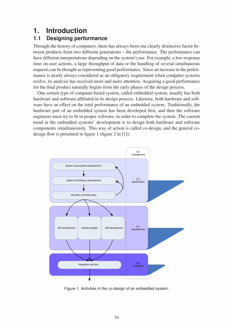
components simultaneously. This way of action is called co-design, and the general co-
design flow is presented in figure 1 (figure 2 in [1]).
Co-
management
Co-
specification
Co-
development
Co-
verification
System requirements development
System architecture development
Allocation and flow-down
SW development HW developmentInterface design
Integration and test
Figure 1. Activities in the co-design of an embedded system.
10
1. Introduction
System requirements development, also known as Requirements engineering (RE), is the
phase which aims at obtaining requirements for the system under design. We define re-
quirements as early stage specifications of what should be implemented, and they can be
descriptions of a system’s behaviour, properties, attributes, constraints and compatibility
issues [2, p. 4]. The following are examples of system requirements [2, p. 4]:
• Features provided for the user (e.g. a spell checker in a word processor)
• General system properties (e.g. the securing of the personal information)
• Constraints for the functionality of the system (e.g. a polling interval for a sensor)
• Constraints in the development of the system (e.g. defining the programming lan-
guage to be used).
Correspondingly, we define Requirements engineering (RE) to include all of the activities
related to discovering, documenting and maintaining a set of requirements for a computer-
based system [2, p. 5]. In this work, we will concentrate on performance requirements.
The performance requirements belong to the requirements class, which is called either
non-functional requirements (NFR) or sometimes quality attributes. In information pro-
cessing systems, the most often used performance requirements relate to throughput and
response times [3]. The typical problems in performance requirements – some already
discussed above – are the following [3]:
• Interactions and conflicts with other requirements: for example, accuracy and speed
may form a trade-off in some systems
• Effect of choosing the development technique – an aspect which is costly to fix after
the development has started
• Global impact to the whole system: in the worst case, optimizing performance can
necessitate modifications in every system module
• Characteristics of the performance vary between different organizations and differ-
ent systems.
System architecture development is sometimes also considered as a separate activity in
the specification phase; it contains the consideration of available hardware components
and the possible constraints set by software components. [1]
Allocation and flow-down means a decision of which functionalities should be per-
formed with hardware, and which with software. Roughly speaking, adding more hardware-
based functionalities means more speed and unfortunately more costs. However, the
adding of software-based solutions also has obligatory costs, such as more software de-
velopment, larger read-only memories (ROMs), and in the worst case the changing of the
selected processor for a more powerful and more expensive version, which also causes
higher energy consumption. Relying on hardware also has problems with a possible need
for redesigning, which is much more complicated on regarding hardware than with soft-
ware. Usually, the partitioning decision should be done at the latest possible time. This
is due to the fact that the understanding of the problem evolves continuously, as the pro-
cess advances. A drawback is that debugging of software is more complicated before the
actual hardware is done; early-stage testing must be done with evaluation boards or so
called stub codes, which mimic the behaviour of the hardware. [4, p. 49]
11
1. Introduction
Nowadays the partition decision is becoming more difficult, because the advancement of
integrated circuits makes the implementation of very complex algorithms possible with
reasonable costs [4, p. 50]. The distinction between software and hardware is also blur-
ring, as hardware designs and software designs look quite alike, they are just used with
different compilers [4, pp. 55–56].
A product’s performance is substantially affected already during these presented steps
forming the co-specification phase. The following phases are co-development and co-
verification. In co-development, the actual development work of hardware and software,
as well as the proper interface between them, are performed. In co-verification, these parts
are integrated and tested. The coordination work of these phases is called co-management.
[1]
Our focus is to propose a new method for the described, early phases of the design
process. To be more specific, we are interested in the performance, as it can be seen in
the next section.
1.2 Motivation
The work aims to provide a new, rather highly abstracted method for system designers in
a multi-processor domain. The method’s purpose is to aid architecture decisions before
prototyping. We will provide a performance simulation for estimating the feasibility of
different design alternatives. The method will attempt to help the selection of the most
favourable ones to be validated with prototypes. After all, we are doing the simulation in
a non-detailed and coarse way. We are favouring simulation, because it is an applicable
way to support the design flow due its modest amount of work. Figure 2 (based on figure
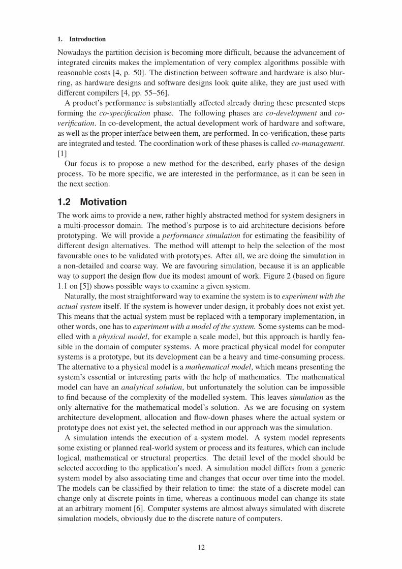
1.1 on [5]) shows possible ways to examine a given system.
Naturally, the most straightforward way to examine the system is to experiment with the
actual system itself. If the system is however under design, it probably does not exist yet.
This means that the actual system must be replaced with a temporary implementation, in
other words, one has to experiment with a model of the system. Some systems can be mod-
elled with a physical model, for example a scale model, but this approach is hardly fea-
sible in the domain of computer systems. A more practical physical model for computer
systems is a prototype, but its development can be a heavy and time-consuming process.
The alternative to a physical model is a mathematical model, which means presenting the
system’s essential or interesting parts with the help of mathematics. The mathematical
model can have an analytical solution, but unfortunately the solution can be impossible
to find because of the complexity of the modelled system. This leaves simulation as the
only alternative for the mathematical model’s solution. As we are focusing on system
architecture development, allocation and flow-down phases where the actual system or
prototype does not exist yet, the selected method in our approach was the simulation.
A simulation intends the execution of a system model. A system model represents
some existing or planned real-world system or process and its features, which can include
logical, mathematical or structural properties. The detail level of the model should be
selected according to the application’s need. A simulation model differs from a generic
system model by also associating time and changes that occur over time into the model.
The models can be classified by their relation to time: the state of a discrete model can
change only at discrete points in time, whereas a continuous model can change its state
at an arbitrary moment [6]. Computer systems are almost always simulated with discrete
simulation models, obviously due to the discrete nature of computers.
12
1. Introduction
Experiment
with the actual
system
System
Experiment
with a model of the system
Physical
model
Mathematical
model
Analytical
solutionSimulation
Figure 2. Different ways to study a system under interest.
A simulation has some major benefits when compared to prototyping. A simulation model
can be executed under arbitrary projected operation conditions, as the control of experi-
mental conditions is better in a simulated environment. Alternative designs or operation
policies can usually be examined and compared with small changes and even in a sin-
gle simulation run, whereas in prototyping, there may be the need for one prototype per
one design proposal. Control over the simulation time is also a remarkable benefit: a
simulation can be driven either in compressed or in expanded time. [5, pp. 76–77]
Our method also includes experimentation with actual systems: we are using data gath-
ered from existing versions to support our performance estimations for the next generation
product. The processing of this data is automated and therefore some of the required steps
in a common simulation study are performed without a user interaction in our method.
1.3 Approach and research questions
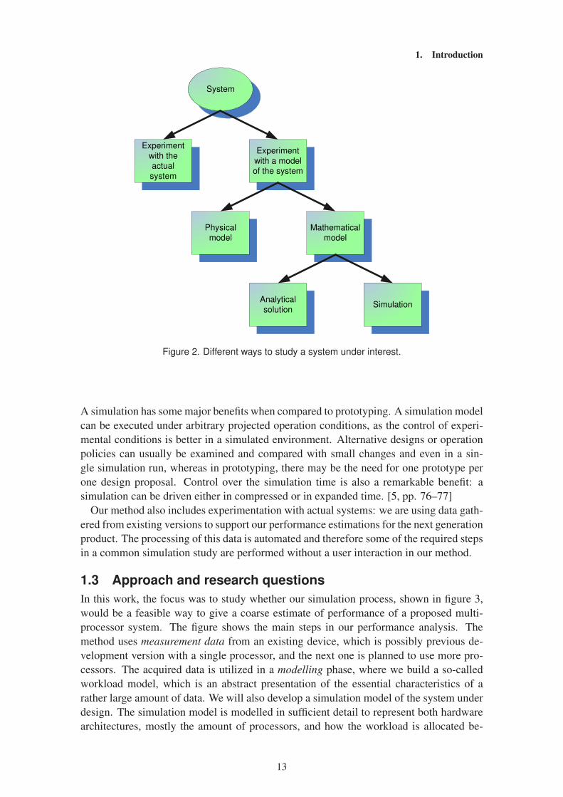
In this work, the focus was to study whether our simulation process, shown in figure 3,
would be a feasible way to give a coarse estimate of performance of a proposed multi-
processor system. The figure shows the main steps in our performance analysis. The
method uses measurement data from an existing device, which is possibly previous de-
velopment version with a single processor, and the next one is planned to use more pro-
cessors. The acquired data is utilized in a modelling phase, where we build a so-called
workload model, which is an abstract presentation of the essential characteristics of a
rather large amount of data. We will also develop a simulation model of the system under
design. The simulation model is modelled in sufficient detail to represent both hardware
architectures, mostly the amount of processors, and how the workload is allocated be-
13
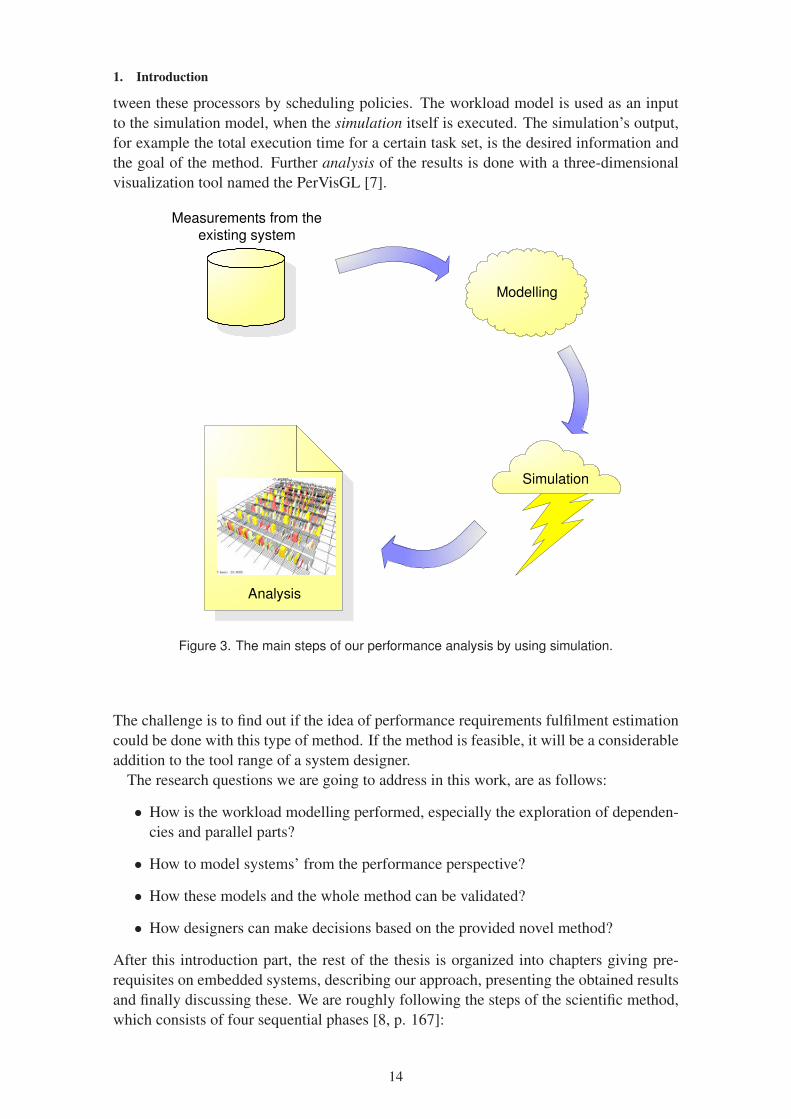
1. Introduction
tween these processors by scheduling policies. The workload model is used as an input
to the simulation model, when the simulation itself is executed. The simulation’s output,
for example the total execution time for a certain task set, is the desired information and
the goal of the method. Further analysis of the results is done with a three-dimensional
visualization tool named the PerVisGL [7].
Measurements from the
existing system
Simulation
Modelling
Analysis
Figure 3. The main steps of our performance analysis by using simulation.
The challenge is to find out if the idea of performance requirements fulfilment estimation
could be done with this type of method. If the method is feasible, it will be a considerable
addition to the tool range of a system designer.
The research questions we are going to address in this work, are as follows:
• How is the workload modelling performed, especially the exploration of dependen-
cies and parallel parts?
• How to model systems’ from the performance perspective?
• How these models and the whole method can be validated?
• How designers can make decisions based on the provided novel method?
After this introduction part, the rest of the thesis is organized into chapters giving pre-
requisites on embedded systems, describing our approach, presenting the obtained results
and finally discussing these. We are roughly following the steps of the scientific method,
which consists of four sequential phases [8, p. 167]:
14

1. Introduction
• Analysis
• Hypothesis
• Synthesis
• Validation.
The analysis phase includes gaining an understanding on components of the problem
domain, and the formulation of a problem description [8, p. 182]. In this work, we will
prepare for the actual approach by reviewing the embedded system’s performance related
aspects from both hardware and software sides, in chapters 2. and 3.. The hypothesis
phase aims to propose a solution to achieve the task objective [8, p. 200]. The synthesis
phase is about implementing the task method [8, p. 220]. Both of these are presented in
the approach chapter (the chapter 4.). The validation phase decides whether the objective
has been achieved [8, p. 280]. Our validation results are presented in the results chapter
(the chapter 5.).
15

2. Embedded Duality – The Hardware PartThis chapter introduces the hardware related areas, which are connected to this work and
thereby gives a basis for our method. At first, we will briefly discuss the special charac-
teristics of embedded systems’ hardware, and then focus on multi-processor architectures
as well as the processing units forming them. The chapter is wrapped up by discussing
performance analysis by simulation methods.
2.1 Characteristics of an embedded hardware
We will begin familiarizing ourselves with the hardware of embedded systems by com-
paring it with a normal personal computer (PC). A PC’s general-purpose processor has
support for a wide range of different level computational applications; on an embedded
system, processing power is ordinarily fitted for a specific task. This is possible due to the
overflowing amount of microprocessor/microcontroller choices for embedded systems.
For personal computers, there are less current processor architecture alternatives. Em-
bedded systems have stricter power constraints than desktop PCs, firstly because they are
often powered by batteries, and secondly because their size may set restrictions on cool-
ing. Due to power saving, an embedded system may be completely interrupt driven; the
processor is in sleep mode and wakes up only upon timer ticks. Environmental conditions,
which an embedded system must tolerate, are sometimes also totally different than for a
PC. Aircraft, space and military applications must stand extreme heat or cold, humidity,
dust and vibration. The amount of resources, for example buses, main memory and mass
storage space, is in practice always smaller in embedded systems, when compared to a
PC. [4, pp. xviii–xxiv]
2.2 Multi-processor systems
When a computer system has more than one “independent” computational unit, it is called
as a multi-processor system. The three main reasons for an ascending popularity of multi-
processor systems are the following: Performance improvements are achieved in a logical
way by connecting multiple processors together, when the capacity of a single processor
is not sufficient. This is probably more cost-efficient that designing a new, more powerful
one. The second reason is the uncertainty about how long the advancement rate can
be kept up by increasing the complexity, silicon and power of a single processor. The
third reason comes from the viewpoint of the software; the trend seems to be towards
parallel operations. Server and embedded areas have a particularly natural parallelism
and utilizing multi-processor hardware is a real advantage there. [9, p. 528]
2.3 Classification of multi-processors
Multi-processor systems can be divided into different classes with at least three sepa-
rate classification rules. The division can be based on the relation between the system’s
instruction and data streams, the system’s memory architecture or the architecture’s hier-
archy.
2.3.1 Division by input and output
The following classic, simple model to categorize computer systems has four classes,
which are still valid despite the model’s high age, although some multi-processors are
hybrids of more than one class [9, 10, p. 529]:
16

2. Embedded Duality – The Hardware Part
1. Single instruction stream, single data stream (SISD): This category includes normal
uni-processors, which process single data element with a single instruction.
2. Single instruction stream, multiple data streams (SIMD): Instructions are dispatched
by a control processor to multiple processors, which have their own data memories.
One example of these kinds of systems is a vector processor, which operates multi-
ple data elements with a single instruction. Some multimedia extensions in current
general-use processors can also be considered as usage of the SIMD method.
3. Multiple instruction streams, single data stream (MISD): A comprehensive MISD-
style commercial processor is not yet built, but some stream processors can be
loosely classified as this since single data stream is operated with successive func-
tional units.
4. Multiple instruction streams, multiple data streams (MIMD): Everything from in-
struction fetching to data operating is handled by each of the multiple processors
themselves. This category is the most used nowadays in general-purpose multi-
processor systems, in contrast to the early multi-processors which applied SIMD.
The benefits of the MIMD systems are cost-efficiency and flexibility. Cost-efficiency is
achieved due to the building of the system with a set of normal microprocessors. Flexibil-
ity appears in cases, where the same system can run a single application at a top perfor-
mance by utilizing all the processors for the same task, and secondly by running several
tasks simultaneously, when required. [9, pp. 529–530]
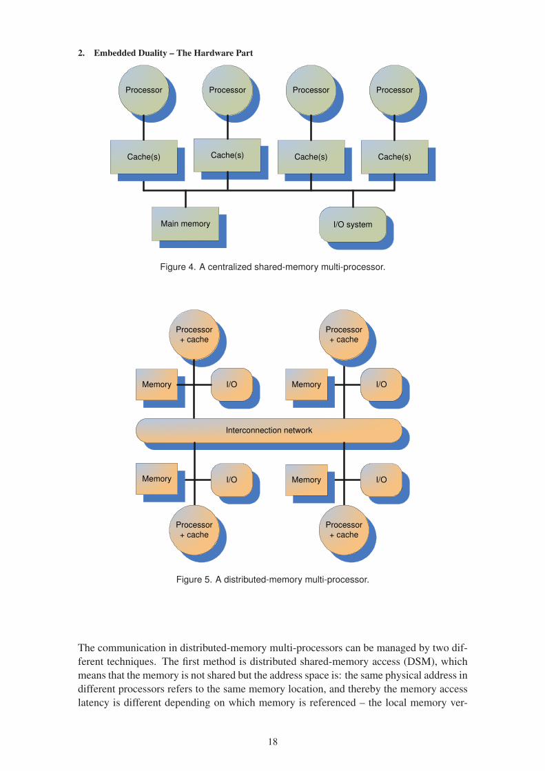
2.3.2 Division by memory architecture
MIMD multi-processors can be further classified by their memory organization. The
first class is centralized shared-memory architectures. Figure 4 (based on figure 6.1 on
[9, p. 531]) shows one example system of this approach. This type has at most a few
dozen processors, which have a shared single centralized memory, as well as a shared I/O
system. On the other hand, the processors have their own caches, which means one or
more levels of very fast and relatively small memory. A bus connects the processors and
the main memory. The relationship to the memory is symmetric for all processors, and
the system can therefore be called a symmetric shared-memory multi-processor (SMP)
and the whole architecture a uniform memory access (UMA), since the memory access
time is identical for each processor. Inter-processor communication is easy due to shared
memory. [9, pp. 530–531]
The second class of MIMD multi-processors, distributed memory architectures, has a
physically distributed memory, like in figure 5 (based on figure 6.2 on [9, p. 532]). This
type is better for larger systems, as there will be problems with bus bandwidth in shared-
memory systems, when the number of processors is increased. This distributed-memory
architecture can be thought to consist of nodes, where every node includes a processor,
memory, sometimes an input/output (I/O) functionality and an interface to the intercon-
nection network. Besides containing one processor, a single node can be a small sym-
metric multi-processor system itself. The advantages of the distributed-memory multi-
processor architecture are that smaller memory bandwidth is sufficient, if it is assumed
that most of the memory accesses will relate to the local memory, and the memory access
latency is also lower. The inter-processor communication is not as simple as with the
shared-memory architectures. [9, pp. 531–532]
17
2. Embedded Duality – The Hardware Part
Cache(s)
Processor
Main memory I/O system
Processor Processor Processor
Cache(s)Cache(s)Cache(s)
Figure 4. A centralized shared-memory multi-processor.
Processor+ cache
Memory I/O
Interconnection network
Processor+ cache
Processor
+ cache
Processor
+ cache
Memory
Memory
Memory
I/O
I/O I/O
Figure 5. A distributed-memory multi-processor.
The communication in distributed-memory multi-processors can be managed by two dif-
ferent techniques. The first method is distributed shared-memory access (DSM), which
means that the memory is not shared but the address space is: the same physical address in
different processors refers to the same memory location, and thereby the memory access
latency is different depending on which memory is referenced – the local memory ver-
18

2. Embedded Duality – The Hardware Part
sus the other node’s memory. This architecture can also be called non-uniform memory
access (NUMA). Still, a processor cannot access every memory location of the system;
some parts require proper access rights. The second communication method has mem-
ories, which are totally isolated from the other nodes’ processors and the architecture is
called a message-passing multi-processor. Converted into real terms, the same physical
address in different processors refers to different memory, respectively. When there is a
need for inter-processor communication, the processor sends a request for some data op-
eration to other processor, which can be thought of being a remote procedure call (RPC).
The destination processor receives the message via polling or interrupts, performs the re-
quested operation and sends the response. The requesting processor waits for the reply
before it continues, so the passing of the message is synchronous. Asynchronous messag-
ing is also possible: the writer of some data is aware that other processors require that data
too, it sends the data directly without waiting for any requests and immediately continues
after the messages have been sent. The nodes in the message-passing multi-processors
can be thought to be separate computers, and the architecture is thereby sometimes called
a multi-computer. A multi-computer can be built with completely separate computers
connected to a local area network, if the amount of the communication is small. [9, p.
533]
2.3.3 Division by the architecture’s hierarchy
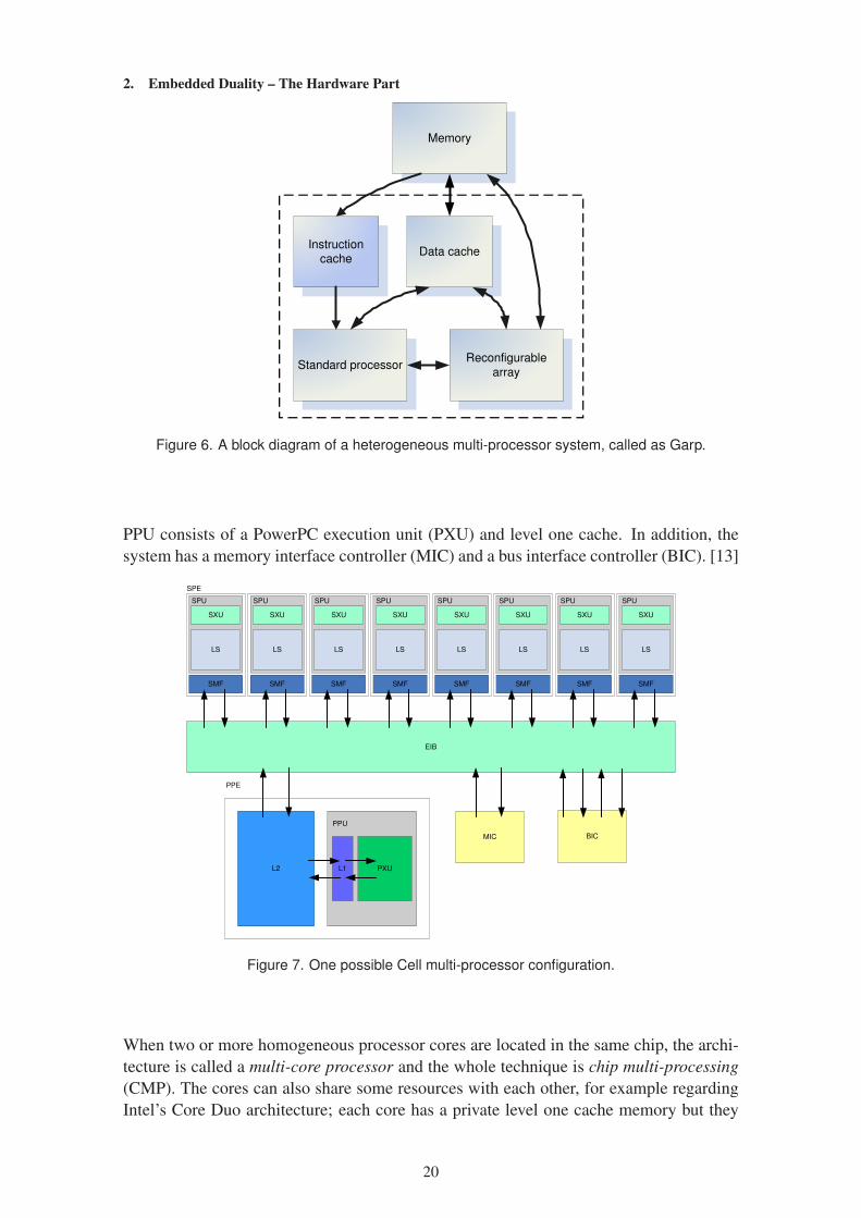
Multi-processor systems can also be divided into heterogeneous and homogeneous sys-
tems. Homogeneous systems have computational units similar to each other, whereas
heterogeneous systems consist of different types of processors: usually one or more cen-
tral processing units and also one or more application specific hardware components.
Embedded systems, related to digital signal processing (DSP), are usually heterogeneous.
Figure 6 (based on figure 1 on [11]) shows the so called Garp architecture, which is a small
heterogeneous multi-processor system where a standard processor is supported by a re-
configurable slave computational unit. In heterogeneous systems, the central processing
unit may be for example, a microcontroller or a programmable digital signal processor,
and the hardware processing element may be an application-specific integrated circuit
(ASIC) or some reconfigurable logic such as a field programmable gate array (FPGA).
One example of an embedded system, which could utilize this kind of configuration, is a
device which performs video or audio decoding, like a present-day mobile phone. [12, p.
1]
One currently interesting heterogeneous processor architecture is the Cell Broadband
Engine. It provides single-chip multi-processing with two different core types which are
called power processor elements (PPEs) and synergistic processor elements (SPEs). PPEs
are responsible for system-wide services such as virtual memory management, handling
exceptions and thread scheduling. SPEs are responsible for most of the data processing.
SPEs perform the computation in an SIMD-style. For example, the configuration of a
Cell chip can consist of one PPE and eight SPEs, like in figure 7 (based on figure on the
page 3 on [13]). The figure shows how each SPE consists of a synergistic processing unit
(SPU) and a synergistic memory flow controller (MFC). Furthermore, each SPU consists
of a synergistic execution unit (SXU) and a local storage (LS). Each SPE has its own
memory flow controller which handles the communication into an element interconnect
bus (EIB) which is used to transfer data between the system memory and local storages.
A power processor unit (PPU) with a level two cache forms a power processor element.
19
2. Embedded Duality – The Hardware Part
Memory
Instruction cache
Data cache
Standard processorReconfigurable
array
Figure 6. A block diagram of a heterogeneous multi-processor system, called as Garp.
PPU consists of a PowerPC execution unit (PXU) and level one cache. In addition, the
system has a memory interface controller (MIC) and a bus interface controller (BIC). [13]
SMF
LS
SXU
SPU
SPE
SMF
LS
SXU
SPU
SMF
LS
SXU
SPU
SMF
LS
SXU
SPU
SMF
LS
SXU
SPU
SMF
LS
SXU
SPU
SMF
LS
SXU
SPU
SMF
LS
SXU
SPU
EIB
L2 L1 PXU
PPE
PPU
MIC BIC
Figure 7. One possible Cell multi-processor configuration.
When two or more homogeneous processor cores are located in the same chip, the archi-
tecture is called a multi-core processor and the whole technique is chip multi-processing
(CMP). The cores can also share some resources with each other, for example regarding
Intel’s Core Duo architecture; each core has a private level one cache memory but they
20

2. Embedded Duality – The Hardware Part
share a level two cache. On the other hand, Intel’s Pentium D architecture also has private
level two caches for each of the cores; however it is still called a multi-core processor, as
the cores reside on the same physical chip. [14, p. 249]
2.4 Building blocks for multi-processor systems
As stated in section 2.3.3, a multi-processor system can be assembled from a set of dif-
ferent kinds of operational units. One significant difference between these units is their
usability for varying tasks – as we move from central processing units to digital signal
processors, field-programmable gate arrays and finally to application-specific integrated
circuits, software-dependency and flexibility decline at the same time. This is illustrated
in figure 8. The above-mentioned units are presented shortly next.
Flexibility
Efficiency
ASIC
DSP
CPU
Figure 8. A comparison between three different computational units. Efficiency on the x-axle
means the energy-efficiency of the unit, when it is performing some task. Flexibility on the y-axle
means the suitability for varying tasks of the unit, including those which are not known of during
the unit’s design-time.
2.4.1 Central processing unit
A central processing unit (CPU), sometimes also called just a processor, or nowadays a
microprocessor when the whole CPU is located in a single integrated circuit, covers a
control unit (CU), arithmetic and logic unit (ALU), input/output interface and internal
memory in the form of registers. The actual random access memory (RAM) is located
externally from the chip as its own component. Interpreting program instructions and
processing data by arithmetic or logic operations are tasks which the CPU handles. The
actual tasks are performed by using software, which utilizes basic operations supported
by the processor – this provides versatility but also causes fairly modest energy efficiency.
[15, pp. 83–84]
21
2. Embedded Duality – The Hardware Part
2.4.2 Microcontroller
A microcontroller differs from a microprocessor by including a CPU, memory, which can
be random-access memory (RAM) or read-only memory (ROM), and other peripherals
like I/O-functionality in the same chip. In other words, a microcontroller is designed to
fulfil a minimum complement of external parts, and this compact package has some ad-
vantages over microprocessor-based systems. A higher level of integration causes lower
cost, as one part replaces many parts. Fewer packages and fewer interconnections enhance
reliability. Since system components are optimized for their environment, and signals can
remain on the same chip, an improved performance is usually achieved. Fast signals do
not radiate from a large board and thereby the so called radio frequency signature is lower.
Due to these aspects, microcontrollers are common and even dominant in embedded sys-
tems. [4, pp. 24–25].
In a multi-processor system, usually either a microprocessor or a microcontroller is in
control of the whole system, and other components can be considered to be slaves to them.
2.4.3 Digital signal processor
A digital signal processor (DSP) is a processor with enhancements and optimizations for
digital signal processing and data transfer oriented tasks. It usually follows the Harvard
architecture, where instruction codes and data have separate memories and at least one
dedicated bus for both. Besides classification into fixed-point and floating-point DSPs,
they can be categorized as general purpose and special purpose DSPs. Special purpose
DSPs can be further classified as algorithm-specific processors performing for example
digital filtering or fast Fourier transforms, and application-specific processors performing
some telecommunications or audio related tasks. [16, pp. 615–618].
When compared with the von Neumann architecture, where the instructions and data
are located in the same memory, the Harvard architecture allows instruction codes to be
of a different size than the data, as well as their addresses. Parallel instruction fetching
and data reading is also possible. [17].
2.4.4 Application-specific integrated circuit
Application-specific integrated circuit (ASIC) is a component, which is designed to con-
stantly perform a specific task by hardware. It has a static structure, where logic gates
and their interconnections are permanently decided on manufacturing. The advantages of
ASICs are their performance, good energy efficiency and small size due to the fact, that
it has only the required amount of logic gates. The disadvantages are a lack of flexibility,
costs for small production batches, long turn-around time, which is the time between the
order and the delivery, and a verification which should be performed before the actual
production. [18]
2.4.5 Field-programmable gate array
Obviously, it would be good if the benefits of the ASICs and general purpose proces-
sors could be combined. In other words, there is a need for a device, which relies on
hardware in performing different tasks but maintains versatility. These types of compo-
nents are called programmable logic devices (PLD). One subtype of PLDs is the field-
programmable gate array (FPGA), which has configurable wiring and logic elements on
one layer, and a personalization memory on the second layer. This personalization mem-
ory is used to configure wiring and logic elements, according to the components’ pro-
22
2. Embedded Duality – The Hardware Part
gramming. These types of FPGAs are re-programmable, but there are also one-time pro-
grammable versions, where the customization is based for instance on fuses. However,
a FPGA has a substantial cost overhead when compared to an ASIC: both the person-
alization memory and configurable logic elements, with their interconnections, have a
remarkable amount of transistors, and depending on which kind and the amount of logic
elements really required, part of the transistors are unused in the current implementation.
[19].
Since the microprocessor’s relatively slow instruction fetch-decode-execute cycle is not
needed, the FPGA performs faster and consumes less energy. Dynamically reconfigurable
systems can switch their configuration during the run-time. This is analogous to a micro-
processor, when it changes a software program under execution. [20]
2.5 Performance gauging – the hardware perspective
Traditionally, processors and whole systems are compared by their performance. The
performance may be thought absolute or relative with other systems. Two classic units of
measurement in the area of performance are MIPS and Dhrystone. The first benchmark,
MIPS, which stands for a million instructions per second, originates from the VAX 11/780
minicomputer, which was the first system which was advertised to perform one MIPS. A
single instruction, however, does not have much to do with actual work performance; the
same work scales into different instruction counts on different architectures. Therefore,
the MIPS is mostly a helpful unit only when comparing different versions of the same
architecture. A more valuable benchmark is the Dhrystone, which is a simple C program
that compiles to about 2000 lines of assembly code. One Dhrystone corresponds to the
execution of 1757 program loops per second. Similarly to the MIPS, the calibration is
inherited from the same VAX machine, which could execute the aforementioned 1757
loops per second. The program is independent of operating system services, but also
has some weaknesses. For example, if this small program fits an on-chip cache of an
embedded system totally, the performance results are naturally skewed. The benchmark
also has difficulties with exploiting parallel performance in the proper way, and compiler
optimizations towards favourable Dhrystone performance are also possible. [4, pp. 26–
27]
2.6 Performance simulations – the hardware perspective
Performance simulators are used for predicting the performance of the given system. In
a computer domain these simulators are almost always software programs written with
high-level languages. Analyzing the performance of a computer system would be nat-
urally easiest to do with direct measurements – however, this kind of method is a post-
design step and rarely contributes directly to the design process of future systems. Pre-
dicting the performance can be completed with analytical models or the performance
simulators, which are usually more detailed and therefore give more valuable informa-
tion to designers. For example, current microprocessors alone are enormously complex
systems and so are the simulators mimicking their performance. The most accurate sim-
ulators work on a so called register transfer level and they simulate the functionality of
basic logic circuits. [21]
A few rather detailed performance simulation solutions are presented next. Although
they actually simulate the complete combination of hardware and software, their low-level
orientation justifies their positioning in the hardware part of this chapter.
23
2. Embedded Duality – The Hardware Part
Rsim can be used to simulate various non-uniform memory access shared memory multi-
processors (see section 2.3.2). The exploitation of instruction-level parallelism (see sec-
tion 3.1) is one of the main interests in the Rsim. The simulator itself is a discrete
event-driven simulator. The events are used to model processor pipelines, caches, mem-
ories and the network connecting the multi-processor architecture. The Rsim models the
competition over system resources and inter-processor synchronization in multi-processor
systems plus speculative execution also in uni-processor systems. Actual program exe-
cutables, compiled and linked for the Sparc V9 systems, can be used as an input for the
simulator; the gathered instructions are processed in a fetch-decode-retire style, which
means that the instruction is dismissed in the third step, in contrast to a real system which
would perform the actual execution as the last step. The output of the simulation has
statistics on the total execution cycles, how many instructions per cycle were achieved,
the usage rate of different functional units in the processor and several readings on the
cache, memory and network operations. [22]
Simics is a simulation platform simulating several different processor architectures at
the instruction-set level. The level of detail is sufficient to run unmodified operating
systems at the top of the simulation platform. The focus is to simulate the full system
consisting of both hardware and the actual software rather than the test code, or even
a distributed system consisting of several nodes and each one of them are simulated.
In the above-mentioned distributed case, simulated nodes could be situated in several
hosts or just in a single one; the network connections in a distributed system can also be
simulated when required. The provided device models are accurate enough to utilize the
real firmware and device drivers. [23]
SimpleScalar is a flexible instruction-set level processor simulator, which can be used in
varying detail. The simplest and fastest model only simulates the instruction set, whereas
the most detailed microarchitectural model has features such as dynamic scheduling,
speculative execution and a multilevel memory system. The SimpleScalar is an event-
driven simulation which uses actual program binaries as its input. [24]
Asim provides modularity to performance modelling. It is a framework where the total
performance model consists of reusable software modules presenting physical compo-
nents. When the user has created the desired performance model by selecting proper
ready-made modules or writing their own modules, the simulation can be executed in
three different ways. A static trace, acquired from another performance model, or a real
system can be fed into the simulator. A dynamic trace works in almost the same way,
but the trace is delivered forward simultaneously while measuring it from another model,
thus saving storage capacity and time. The instructions can then finally be fed into the
simulator from a program binary. [25]
24
3. Embedded Duality – The Software PartThis chapter discusses topics from the software side of embedded systems. Once again,
the focus is placed on areas affecting the performance. Without underestimating the actual
software applications’ effect on the system’s performance, in this work we will maintain
quite a neutral sentiment towards them and focus more on the operating system level.
Translated into real terms, we will handle programs as processes and threads and give
special attention to their scheduling. We will finally discuss performance from the soft-
ware perspective and how it can be estimated by the means of workload modelling and
simulation.
3.1 Concepts of processes and threads
A process consists of a running program itself, and its state. A process is independent
from other processes, although processes can exchange information. Thereby, utilizing
several processors with several processes is a quite straightforward matter. The concept of
a process is also widely used in uni-processor systems, when programs share a single uni-
processor computer. Processes are executed in short time slices, known as time-sharing,
so it seems to the user that they are running simultaneously. Process state information is
used when a process switch or a context switch occurs: the state of the preceding process
is saved and the following is correspondingly restored. [9, p. 469].
The three most essential states for a process are running, ready and blocked. A running
process is logically a process that is currently under execution. A ready process is all
set for execution and waiting for processor assignment. A blocked process is waiting for
some event, an I/O-event completion for example. [26, p. 55].
Processes, which share their code and most of their address space, are called threads, as
shown in figure 9. Threads are also used with uni-processor systems, but a multi-processor
system can utilize them perfectly. For a multi-processor system with n processors, there
must be at least n processes, threads or a combination of these two, in order to system run
at full throughput. Threads are usually created by the programmer, or in some cases the
compiler can optimize a code by generating threads automatically. The parallelism here is
called thread-level parallelism (TLP), and when compared to instruction-level parallelism
(ILP), the ILP is handled mostly by hardware and it relates to a single instruction at a
time, whereas thread-level parallelism relates to a substantial amount of instructions. [9,
p. 272]
The utilization of threads within a single processor, called multi-threading, is divided
into different approaches. Fine-grained multi-threading is a version which switches be-
tween threads on each instruction and skips threads, which are not ready to run at that
precise moment. Practically, this kind of multi-threading requires support for thread
switching at every clock cycle. The main advantage is that the system can execute other
threads when some of them stall. On the other hand, an individual thread’s execution is
constantly interfered with by other threads. Coarse-grained multi-threading does switch
between threads but only on costly long stalls. An execution of an individual thread is
more continuous, but the throughput of the system is affected by shorter stalls. In si-
multaneous multi-threading (SMT), both the TLP and ILP are exploited simultaneously.
Various functional units of a processor are used to execute instructions from different
threads in a single clock cycle. The SMT demands the ability to fetch instructions from
different threads and also sufficient buffer spaces. [9, pp. 608–610]
Some operating systems, for example Linux, do not draw a major difference between
25

3. Embedded Duality – The Software Part
Process 1 Process 2 Thread 1 Thread 2
Address space x
Address space y
Address space z
Figure 9. The greatest difference between processes and threads is the sharing of address
spaces.
processes and threads. Linux threads have all the features such as normal processes,
however part of their resources are shared and therefore they are called as lightweight
processes. [27, p. 80]
3.2 Scheduling levels and objectives
The assignment of physical processors to processes, in order to processes accomplish
work, is called processor scheduling [26, p. 249]. Respectively, a scheduling algorithm is
a set of rules that determine the task to be executed at a particular moment [28]. One can
say that the distributed system resource here, the CPU time, is a type of renewable one.
However, its handling is not a trivial task as we will see in the following sections.
The scheduling, performed by an operating system, can be divided into three differ-
ent levels. High-level or long-term scheduling, also called job or admission scheduling,
is used to determine jobs which shall be allowed to compete actively for the system re-
sources. Once a job is admitted to the system, it becomes a process or a group of pro-
cesses. Intermediate-level or medium-term scheduling determines which processes shall
be allowed to compete for the CPU and brought to the main memory by swapping them
from the mass storage; the method used is suspending and activating processes depending
on fluctuations in the system’s load. The benefit of this kind of scheduling is a smoother
system operation and contribution to certain performance goals. Low-level or short-term
scheduling determines the assignment of ready processes to the CPU. This is called dis-
patching and the module responsible for low-level scheduling is correspondingly called
the dispatcher. The relationships between different process states (see section 3.1) and
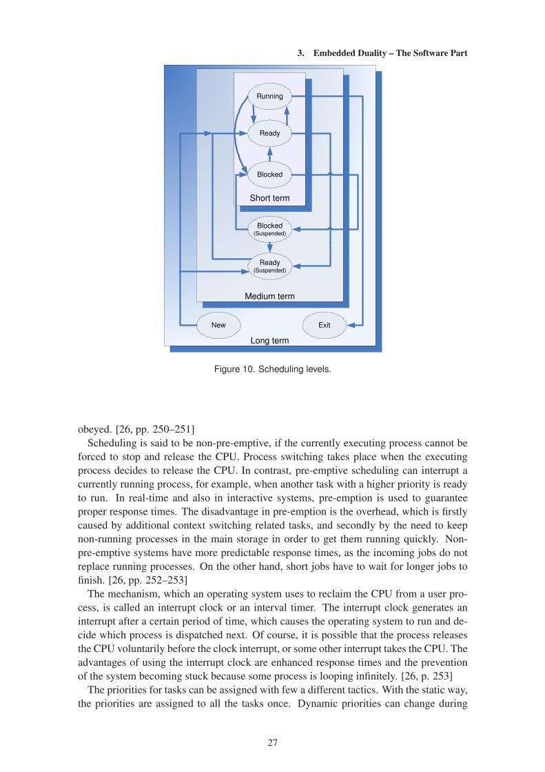
scheduling levels are presented in figure 10 (based on figure 9.2 on [29, p. 396]). [26, 29,
pp. 249–250, pp. 394–398]
Scheduling has several general objectives. Scheduling should be fair – all processes
should be treated likewise. The number of serviced processes per time unit should be
maximized, whereas the response times should be minimized. The load of the system
should not have an effect on the scheduling, and the overheads caused by the scheduling
should be minimal. Resource utilization should be balanced, and the given priorities
26
3. Embedded Duality – The Software Part
New Exit
Blocked(Suspended)
Ready(Suspended)
Running
Ready
Blocked
Short term
Medium term
Long term
Figure 10. Scheduling levels.
obeyed. [26, pp. 250–251]
Scheduling is said to be non-pre-emptive, if the currently executing process cannot be
forced to stop and release the CPU. Process switching takes place when the executing
process decides to release the CPU. In contrast, pre-emptive scheduling can interrupt a
currently running process, for example, when another task with a higher priority is ready
to run. In real-time and also in interactive systems, pre-emption is used to guarantee
proper response times. The disadvantage in pre-emption is the overhead, which is firstly
caused by additional context switching related tasks, and secondly by the need to keep
non-running processes in the main storage in order to get them running quickly. Non-
pre-emptive systems have more predictable response times, as the incoming jobs do not
replace running processes. On the other hand, short jobs have to wait for longer jobs to
finish. [26, pp. 252–253]
The mechanism, which an operating system uses to reclaim the CPU from a user pro-
cess, is called an interrupt clock or an interval timer. The interrupt clock generates an
interrupt after a certain period of time, which causes the operating system to run and de-
cide which process is dispatched next. Of course, it is possible that the process releases
the CPU voluntarily before the clock interrupt, or some other interrupt takes the CPU. The
advantages of using the interrupt clock are enhanced response times and the prevention
of the system becoming stuck because some process is looping infinitely. [26, p. 253]
The priorities for tasks can be assigned with few a different tactics. With the static way,
the priorities are assigned to all the tasks once. Dynamic priorities can change during
27
3. Embedded Duality – The Software Part
scheduling, and a mixed scheduling algorithm contains varying priorities for some tasks
and static for the rest. [31]. The assignment can be performed by the operating system
or it may come from outside the system. Static priorities have a low overhead, but they
do not respond to changes which would require adjustments. An overhead caused by
dynamic priorities is usually compensated for by improved responsiveness. [26, p. 253]
3.3 Scheduling algorithms from a uni-processor viewpoint
Uni-processor scheduling strategies are discussed in this section, in order to ease the un-
derstanding of their multi-processor versions. Scheduling can be implemented with sev-
eral different algorithms. First-in-first-out (FIFO), also known as first-come-first-served
(FCFS) scheduling, is a simple non-pre-emptive discipline which dispatches processes
based on their arrival time to a ready queue. It has quite predictable response times, but
long jobs force short jobs to wait, as well as unimportant jobs make more important jobs
wait. FIFO scheduling can be used as a part of other scheduling algorithms, for example
on decisions among processes with the same priority. [26, 29, pp. 254–255, pp. 403–406]
Round robin (RR) scheduling works partially like the FIFO, but it only gives a slice of
the CPU time, so called quantum to each process at a time. Processes, which do not finish
their execution before the quantum has passed, are pre-empted and placed at the back of
the ready list. Round robin has reasonable response times in time-sharing environments.
The quantum size can be fixed or variable; a too small quantum size causes the context
switching overhead to grow larger than useful work, whereas a too long quantum makes
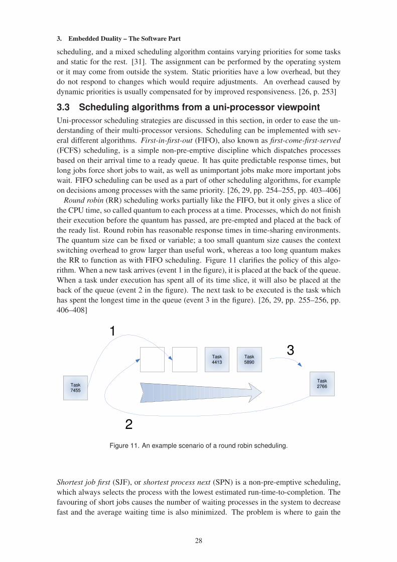
the RR to function as with FIFO scheduling. Figure 11 clarifies the policy of this algo-
rithm. When a new task arrives (event 1 in the figure), it is placed at the back of the queue.
When a task under execution has spent all of its time slice, it will also be placed at the
back of the queue (event 2 in the figure). The next task to be executed is the task which
has spent the longest time in the queue (event 3 in the figure). [26, 29, pp. 255–256, pp.
406–408]
Task
4413
Task
5890
Task 7455
Task
2766
1
2
3
Figure 11. An example scenario of a round robin scheduling.
Shortest job first (SJF), or shortest process next (SPN) is a non-pre-emptive scheduling,
which always selects the process with the lowest estimated run-time-to-completion. The
favouring of short jobs causes the number of waiting processes in the system to decrease
fast and the average waiting time is also minimized. The problem is where to gain the
28

3. Embedded Duality – The Software Part
estimates – in environments, where the same jobs come into execution in a periodic way,
there may be good estimates, but the proper estimates are often impossible to obtain. SJF
does not apply to time-sharing systems because it is non-pre-emptive. [26, 29, p. 257, pp.
408–410]
The pre-emptive counterpart of the SJF is called shortest remaining time (SRT) schedul-
ing. The SRT may replace a currently running process with a process, which has a smaller
run-time estimate. The replacement of a nearly completed process with only a slightly
shorter job can be avoided by setting a threshold value, which guarantees that processes
closing their completion can continue to execute uninterrupted. This algorithm requires
the recording of elapsed execution times, which causes some overhead. [26, 29, pp. 257–
258, p. 410]
Highest response ratio next (HRN or HRRN) is a non-pre-emptive scheduling which
calculates a priority-ratio for processes as a sum of the elapsed waiting time and the
required service time, which is divided by the service time. The denominator causes
shorter jobs to be preferred, but the increase in waiting time, called aging, increases the
ratio and therefore guarantees that longer jobs will also be executed. The weakness of the
HRRN is the need for service time estimates. [26, 29, p. 258, p. 412]
A scheduling algorithm called multilevel feedback queues consists of a queuing net-
work, where a new process is placed at the back of the highest level queue, which has
the highest priority. When a process goes through this queue in FIFO-style, and does not
complete its execution in the given time quantum, it is dropped into the lower level and
lower priority queue. Long processes go through the whole network, until they are finally
completed in the lowest level, which is usually implemented in RR style. This method
is based on imposing a penalty on processes which have run too long, although the time
quantum can increase at the lower levels. The methods advantage is that service time
estimates are not required. [26, 29, pp. 259–261, pp. 412–414].
3.4 Multi-processor scheduling
Scheduling can be thought to be the most essential factor, when a user reviews the per-
formance of an interactive system. When we are moving from a uni-processor system to
a multi-processor version, its importance is emphasized even more. Particularly, keeping
all the processors as utilized as possible is one of the common scheduling problems in a
multi-processor domain. Scheduling related aspects therefore play an important role in
this work.
When scheduling multi-processor systems is considered, in addition to the actual dis-
patching of a process and the use of time-sharing on an individual processor, the assign-
ment of processes to processors must be handled. A static assignment is the simpler
alternative: a process is assigned to one processor for its whole execution span. The dis-
advantage is that one processor may be idle, while other processors have lot of assigned
tasks waiting. A dynamic assignment bypasses this problem because the execution for
the same process can take place in an arbitrary processor; however the repetition of the
assignment during scheduling creates some overhead. Implementation for the assignment
can be performed with master/slave or peer architectures. The master/slave architecture
uses a particular processor to execute the key kernel functions of the operating system,
such as scheduling. In this approach, the master processor can become a bottleneck for
the whole system’s performance and its failure will also halt other processors. Peer archi-
tecture can execute these kernel functions on any processor and therefore the processors
29

3. Embedded Duality – The Software Part
self-schedule their tasks. This approach must have some kind of synchronization and con-
flict resolution, as processors may compete for same processes. An intermediate solution
is to perform scheduling on a subset of processors. [29, pp. 440–441]
Methods for the actual implementation of the multi-processor scheduling include for
example load sharing, gang scheduling, dedicated processor assignment and dynamic
scheduling. Load sharing uses a global queue of ready threads, which causes an even
distribution of work to all processors, and also bypasses the problem of idle processors if
there is work available. Scheduling decisions are made in a non-centralized way; the op-
erating system is run on an available processor to select the next thread for it. Arranging
the queue can be based on basic FCFS, or jobs with the smallest number of unscheduled
threads can be alternatively executed first. The problems in this method are the syn-
chronization of the global ready queue, extensive swapping of the cached data because
pre-empted threads are often forced to continue their execution on different processor,
and a distortion on the execution times of dependent threads, which would need to be
executed concurrently. [29, pp. 444–445]
The performance bottleneck of the load sharing methods is caused by interacting threads
or processes, when they are executed in separate time slots. Repetitive and unnecessary
context switches occur because the synchronization points are reached at different times.
This can be avoided through gang scheduling, also called group scheduling, which sched-
ules closely related processes and threads to be executed in parallel. A performance gain
comes from reduced context switching, which is consequence of reduced synchroniza-
tion blocking – threads have a possibility to catch up to synchronization points in a much
shorter time interval due to parallel execution. The scheduling related overhead is smaller,
because decisions are made for a group of jobs at the one time. Resource allocation is
also more efficient, because the cooperating threads are probably interested in the same
resource, which can be accessed by several threads via their cooperation. [29, 30, pp.
446–447]
A dedicated processor assignment does not use pre-emption or multiprogramming at
all; instead, a group of processors is dedicated to the application. In this approach, ap-
plications must be able to dynamically control the number of processes, depending on
the amount of the assigned processors. Processes and threads run on the same processor
until their completion – an absence of context switching causes improved performance.
A lack of multiprogramming is justified in larger systems, because the single processor’s
blocking does not substantially affect the efficiency of the whole system. [29, 31, p. 447]
Equally, in dynamic scheduling, the number of threads is dynamically controllable by
applications. A dynamic allocator primarily fulfils new requests with unallocated proces-
sors. If there are not any, allocated but currently unused processors are used next. The
last possibility is to enforce equipartition by pre-empting processors from an application
with the largest amount of processors. [29, 32, p. 449]
3.4.1 Algorithms especially for embedded systems
We will next look at multi-processor scheduling models, which are particularly utilized
in embedded systems. They focus on task-level parallelism. All of these models are re-
stricted to fulfil non-pre-emptive scheduling: tasks are executed as long as they wish once
they are started; there is no forced context switching (see section 3.2). This restriction
is justified with the implementation overhead caused by the pre-emption, which is un-
wanted in embedded time-critical systems. A computational task is called an actor; actors
30
3. Embedded Duality – The Software Part
are types of sub-functions, which jointly carry out some larger function. The scheduling
of these actors starts from the processor assignment step, which means choosing the pro-
cessor where an actor will be executed. The next task is the actor ordering step, which
means the order that these actors are to execute when considering just a single proces-
sor. Finally, the execution start time, called firing, is determined for each actor. Different
strategies can be classified based on which of the above-mentioned tasks are performed at
the compile-time and which at the run-time. A fully-static strategy does each of the three
tasks at the compile time. A self-timed strategy determines the start times at run-time,
by communication between the processors in order to get tasks synchronized, but the or-
dering and allocation to processors are decided during the compiling. A static allocation
scheduling only performs processor assignment step at the compile time. If all scheduling
decisions are made at the run-time, the strategy is called fully dynamic. These are the four
main classes; there are also two more modifications of these. A quasi-static technique has
a small amount of run-time control, which handles ordering in the data-depended parts of
the execution. An ordered-transaction strategy is almost like a self-timed approach, but
the inter-processor communication order is determined at the compile time. [12, 33, pp.
55–67]
A fully-static (FS) strategy is used in systolic arrays and in very long instruction word
(VLIW) processors. The timing of operations is known at the compile time, and this
is enforced during the run-time, either by the programs themselves or by a program se-
quencer. The goal is usually to minimize the total schedule length, the make-span of the
schedule, which also minimizes the idle periods for each processor. This strategy can fur-
ther be divided into blocked and overlapping schedules. A blocked schedule completes
the whole iteration before proceeding into the next one; the dependencies between suc-
cessive iterations can thereby be ignored. The length of the critical path – which is the
longest delay free path – specifies the minimum iteration period T for a blocked schedule.
Some of the FS scheduling heuristics also take into account inter-processor communica-
tion (IPC), which causes costs when the processors need to communicate with each other.
The enhancements to blocked schedules are unfolding and retiming. The unfolding strat-
egy improves blocking schedules by scheduling the N iterations together. The number
of replicated iterations N, which is called the blocking factor, also increases usage of the
program memory by the same factor. In the retiming strategy, delays are manipulated
in order to shorten the critical path, which directly affects the minimum of the iteration
period. The overlapping strategy interleaves successive iterations, and is capable of lower
iteration periods than blocking schedules, even when unfolding and retiming are used.
[12, pp. 57–62]
When actor execution times are not known beforehand, in other words when execution
times are varying, the fully-static strategy can be used with worst-case execution times.
This is obviously an inefficient way, and secondly, the precise worst-case estimates may
be unknown. In a self-timed scheduling (ST), the fully-static schedule is first built based
on execution time estimates. Timing information is discarded; processor assignment and
the ordering of the actors are instead used as such. Some of the actors are so called
communication actors, performing send or receive operations; these are executed after
all the input data is available. Sending actors are also blocked if the target buffer is full;
correspondingly, receiving actors are blocked if the source buffer is empty. The sender-
receiver synchronization is thus performed at the run-time; the disadvantage is a higher
interprocessor communication cost due to this synchronization, when compared to the FS
31
3. Embedded Duality – The Software Part
strategy. In FS scheduling, there are typically only a few processor cycles required for
the IPC, whereas in ST scheduling, the amount is dozens, unless special hardware for
flow control is used. On the other hand, ST scheduling simplifies the compiler software
because it does not have to adjust exact timing. [12, pp. 62–64]
A fully dynamic approach makes all the scheduling related decisions at the run-time. It
has a very general applicability for various kinds of tasks; however it also has disadvan-
tages such as the cost of performing these run-time decisions by special purpose hardware,
like in superscalar processors, or by kernels running on one or more processors. Another
disadvantage is that a dynamic scheduler usually only performs locally optimal decisions.
[12, pp. 64–65]
A quasi-static scheduling is feasible with data-dependent execution times, which is
generally caused by data-depended control structures, such as conditionals and data-
dependent iterations [12, pp. 65–67]. The firing of all nodes is decided at the compile
time, but they are adjusted, when absolutely necessary, also at the run-time. Execution
and scheduling progresses normally, until it reaches some data-dependent control struc-
ture. At this point, for example in the case of a branch with two unequal execution times, a
run-time scheduler generates two different schedules, one for each branch. The difference
here is that the initial pattern of processor availability is arbitrary. Obtained schedules are
adjusted by padding them with idle periods, in order to make the processor availabil-
ity patterns symmetric. If some other kind of synchronization between the processors is
present, padding may not be required. If there is probability information available, about
which branch will be executed, the higher probability branch can be scheduled first, and
the second branch will be padded to fulfil the same pattern of processor availability. The
absolute time values do not have to be identical, just the pattern. Finally, when this data-
dependent part of the schedule is completed, the original schedule can continue normally.
[34].
3.4.2 Scheduling in shared memory systems
Fixed-priority scheduling algorithms in shared-memory multi-processor systems can also
be divided between two methods: partitioned and non-partitioned. With the partitioned
method, the execution of all instances of a task takes place on the same processor, which is
already chosen before the run-time, by a partitioning algorithm. The non-partitioned ver-
sion, which is also known as “dynamic binding” and “global scheduling”, allows the task
to be executed on any processor. This also includes the case when the task is continued
after pre-emption. The non-partitioned method has less pre-emptions, since high-priority
processes can utilize possible idle processors, rather than replace the executing task on
the same processor. Since the partitioned method is guided by worst-case execution time
estimates; whenever the actual execution times may be substantially lower than this, the
utilization of processors remain low and would be better with a non-partitioned method.
[35]
3.5 Performance gauging – the software perspective
In addition to the aspects mentioned in section 2.5, real benchmarking includes application-
specific measuring. In real-time embedded systems, the fluency of context-switching and
interrupt handling are two components required for a good real-time performance. The
best results can be achieved with benchmark suites based on real-world algorithms. [4,
pp. 28–31]
32
3. Embedded Duality – The Software Part
The over-designing of hardware could usually be avoided with proper software tuning,
and the applicable points of the software can be pointed out with performance testing.
The basic operation in performance testing is the measurement of the time consumed in
the execution of a function. The execution is generally a nondeterministic process, factors
such as the contents of instruction and data caches, operating system task loading, inter-
rupts and other exceptions and finally data-processing requirements in the function cause
diversity in the execution time. Therefore, the statistical measuring of minimum, maxi-
mum, average, and cumulative execution times is recommended. The execution times can
basically be measured by identifying the memory addresses of the entry and exit points
of the desired functions from the link map file. By observing the address bus, and record-
ing the times when the corresponding addresses are detected, the execution time can be
calculated. The difficulties in this technique include the calls of other functions inside the
interesting one, with possible recursion, and interrupts whilst the function is executing;
both aspects must be noticed in order to obtain correct results. Fortunately, the com-
mercial tools built for performance testing can usually handle these kinds of problems.
On-chip counters (see section 3.7.4) can be also used as performance measurement tools,
for example to count elapsed time. [4, pp. 201–205]
3.6 Performance simulations – the software perspective
As explained in section 2.6, the division between hardware- and software-oriented perfor-
mance simulators is a matter of opinion, as the performance is affected by both of them.
This section wields simulators more from the side of software.
One approach in performance simulations is to have separate models for the applica-
tions to be executed, and for the hardware itself. It is even possible to use two different
modelling languages to represent these two models; for example the Unified modelling
language (UML) for the applications and SystemC modelling language for the hardware.
The applications can be modelled by utilizing algorithm descriptions or the source code.
To allow the execution of the applications modelled in a different language than the sys-
tem, a proper interface between the models must be implemented. [36]
It is also possible to estimate the performance with a much higher level of abstraction.
This usually means more abstraction to the hardware part. One practical and efficient way
to simulate the performance of a computer-based system is to abstract their load somehow
and then to consume it in an abstract simulated environment. The input data processing –
called workload modelling – is an important step in this kind of simulation.
Simulation naturally has also its disadvantages and pitfalls. The development of a sim-
ulation model takes time and resources, the output of the simulation is just an estimate
of the true system’s characteristics and often the simulation results are given much more
confidentiality than justified. [5, p. 77]. Especially in cases where a modelled system is
only just at the proposal phase, its validation cannot be performed against any real world
system, which causes an uncertainty in the results.
3.7 Workload modelling
Workload modelling can be described as an attempt to create a simple and general model,
which can be used to generate synthetic workloads for systems that are under some kind of
evaluation. One typical case, where a workload is required, is a performance analysis of
computer-based systems. The workload presents the software that is meant to be executed
in the actual system. A synthetic workload should be as similar as possible with the
33
3. Embedded Duality – The Software Part
real workload. A good workload model also makes it possible to generate various kinds
of workloads with slight modifications. The workload modelling is usually based on
measurements from the system of interest; the record or data log of workload-related
events is often called a trace. An example of a single trace entry could consist of the
arrival time of a job, where it was executed and what resources it required. This type of
measurement-based modelling began strongly as late as the 1990’s, when it was noticed
that mathematical analyses, based on assumptions, differ notably from real workloads.
[37, p. 10]
Workload modelling is about generalization and simplification. Measurements are al-
ways limited, the measuring process may be inconvenient or costly to realize, and the
measurement instrumentation may cause an overhead and therefore disturb the results.
The collected data is valid under strict conditions, for example, data which is collected
from a 128-node supercomputer does not apply directly to 64- or 256-node supercom-
puters, but with a valid model based on the mentioned measurement, this limit can be
overtaken. Models can also be executed with different seeds for random numbers, and
therefore the statistical conditions remain the same, as required in the calculation of con-
fidence intervals. This is not possible within a single trace. [37, pp. 10–12]
3.7.1 Alternative approaches in workload modelling
There are two different approaches to analyze or evaluate a system design with a measured
workload. A simulation can be driven with a traced workload directly or alternatively
with a model, which has been created from the trace. When using a trace directly, which
means the measured workload, the system is going through a realistic test as the workload
is accurate, and the person performing the analysis does not have to know every detail
about the workload. On the other hand, a generalization to other systems or other system
configurations may be a problem, because different systems with different architectures
are probably unable to use the same trace at all. Information on the circumstances, when
the trace was collected, should also be known. [38]
Workload models have some advantages, when compared to traces [38]:
• Models provide full information of workload characteristics to the modeller, for
example, a correlation of different parameters is visible
• Model parameters can be changed one at a time, whereas manipulating traces with
such an accuracy is challenging at the very least
• Models are not affected by the policies and constraints of the recording site
• Models enable the easier cleaning of so called bogus data, which can be for example
killed jobs, which are executed multiple times before completion
• Workload modelling also increases understanding on the system requirements and
can lead to new designs.
3.7.2 Creating a workload model
The creation of a workload model is based on data analysis; instead of trusting just the
statistical methods, which are the primary tools in this task, it is desirable to also use
graphical methods and common sense. Depending on the planned usage of the workload
model one can choose between two different model types [37, pp. 15–16]:
34
3. Embedded Duality – The Software Part
• A descriptive model tries to describe just the measured phenomenon
• A generative model tries to articulate the process that originally generated the mea-
sured workload.
Descriptive modelling usually relies on creating a statistical summary of the observed
workload. In most cases, the observation period should be as long as possible. Once
the model is created, the synthetic workload can be obtained by sampling the distribution
functions of the model. The proper distribution can be selected not by just fitting its
shape, but also by some other feature, such as moments. Capturing a certain feature from
the observed workload is sometimes sufficient, but when the effects of other features are
unknown, it is safer to try the modelling as complete as possible. The validity of the
model is dependent on many factors; if one attribute is modelled with great precision and
other ones are formed by baseless assumptions, the validity is clearly not the best. The
advantage of generative, which is also called indirect modelling, is that the workload-
generation process can be manipulated, in order to obtain different types of workloads,
which are still correct. [37, pp. 15–16]
The structure of a workload model depends on its purpose; the following examples are
given in [37, pp. 5–6]. For scheduling problems, the relevant, sufficient attributes for the
model are the arrival and running times for each job – there is no need for very specific
details on what happens during the execution of the job. If the memory aspects of some
system are also being examined, there is usually the need for total memory consumption
and also a locality of reference. When I/O-processes are taken into consideration, the
appropriate attributes are a distribution of I/O sizes and how they interleave with the
execution. A typical case is that either computation or I/O is the scope of the evaluation,
and the other one is modelled in a very abstracted way – just spending some time between
the more interesting tasks. Parallel jobs can also have the number of processors used as
an additional parameter. In contrast, when new microprocessor architecture is evaluated,
the workload model must be much more specific. This type of model requires details
such as instruction mix, instruction count between branches, loop sizes and dependencies
between the instructions for instruction-level parallelism [39].
3.7.3 Types of workload
The workload itself can be classified into two different types [37, pp. 7–8]:
• A static workload has a certain amount of work, it gets completed at the end
• A dynamic workload contains jobs that are arriving all the time, and it will never
get finished.
Because dynamic workloads include an arrival process, it must be also characterized and
implemented properly which causes extra effort. A dynamic workload model should in-
clude all possible jobs and also their realistic frequency of occurrence. The difference
between input distribution and “live system snapshot” must be noticed: even if the input
has substantially more shorter jobs, a random snapshot may give an erroneous impression
that longer jobs would be more common. This originates from the fact that the longer jobs
naturally stay in the system for a longer period of time. The state of the system may affect
the evaluation; a clean system may have a better performance than a system which has
been executing a dynamic workload. Aging may also be present in a system; for example,
35
3. Embedded Duality – The Software Part
memory leaks are one source for this kind of property in computer systems. Therefore, a
dynamic workload model is usually the best representation of a real workload. [37, pp.
7–8]
3.7.4 Gathering data for modelling
As mentioned before in section 3.7, workload modelling is typically based on measured
data. In some cases, data may be already available: for example, larger server machines
usually log requests and other activities. However, these logs may not have a sufficient
level of detail. If the data must be collected, it can be done by instrumenting the system
in a way that its activities can be recorded. The required facilities should not modify the
behaviour of the system at all; however, this can be problematic to implement. Depending
on the instrumentations interaction with the actual system, the instrumentations can be
divided into the following classes [37, pp. 18, 25–26]:
• A passive instrumentation does not modify the system itself
• An active instrumentation is integrated into the system, either at the design phase or
afterwards.
Passive instrumentations are implemented with external components, which monitor sys-
tem activity without interfering with it. For example, listening nodes can be added to
the network in communication networks. These can record logs about the activity of the
network, without sending any data into it. An example of an active instrumentation could
be a microprocessor, which includes counters used to write down the amount of multipli-
cation, division, load and store operations. These can be utilized when the workload is
being modelled. [37, pp. 18, 25–26]
With active instrumentations, their interference should be as minimal as possible, and
data buffering is one possible technique to reduce it. It means that a note of an event
is stored in an internal buffer, and its output takes place later, in order to minimize the
overhead caused by the data transfer [37, pp. 18, 26–27]. The so called instrumentation
uncertainty principle has the following aspects [40]:
• Instrumentation causes perturbation into the system state
• Execution phenomena and instrumentation have a logical connection
• Volume and accuracy are contrary to each other.
Another method to manage instrumentations interference is to create models of pertur-
bations, and then use them when approximating the traces, as they would be without
instrumentation. This is called as perturbation analysis, and it consists of two phases:
execution timing analysis and event trace analysis. The goal of the execution timing anal-
ysis is to adjust the trace event times, so that perturbations are removed. This is based
on the measured costs of instrumentation. In event trace analysis, the sequence of events
is adjusted based on event dependencies, in order to remove reordering caused by the
instrumentation. [40]
One possible interference reduction technique is dynamically scalable instrumentation.
The instrumentation can be inserted and altered during the execution of a program. This
is implemented by modifying the binary image of the program while it is running. The
volume of collected data is controlled by collecting only the information required at the
36
3. Embedded Duality – The Software Part
moment, and also by adjusting the sampling rate. Instrumentation can be added in defined
locations of application, called points. Instrumentation operations, which alter counters
and timers, are called primitives. Boolean expressions, which affect instrumentation exe-
cution, are called predicates. Manual invocation is also possible. [41]
If the amount of collected data becomes too great, it is usually recommended to take
samples over a longer period of time, than shorten the duration of the whole process.
Anyway, sampling has some problems: choosing a constant interval between the samples
can cause an aliasing effect on periodic data, and on the other hand, random sampling can
also hide some characteristics of the data. If the data includes some internal structure, the
sampling strategy should be constructed so that such structures are preserved. [37, p. 27]
One solution, providing dynamic instrumentation support for Linux operating systems,
is named SystemTap. If a Linux kernel supports SystemTap and has proper debugging
information included, the core of the operating system can be instrumented dynamically
during the run-time. Probes are written with relatively simple scripting language. After
compilation of a probe, it is injected into a kernel binary image. Besides the function
entry and exit points, arbitrary statements are opportune probe positions. Whereas the
probe’s own variables can be used for example to count the amount of calls to a particular
kernel function, whilst local variables in the target system can also be traced. [42]
37
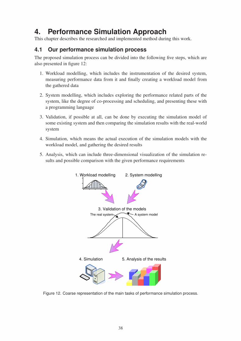
4. Performance Simulation ApproachThis chapter describes the researched and implemented method during this work.
4.1 Our performance simulation process
The proposed simulation process can be divided into the following five steps, which are
also presented in figure 12:
1. Workload modelling, which includes the instrumentation of the desired system,
measuring performance data from it and finally creating a workload model from
the gathered data
2. System modelling, which includes exploring the performance related parts of the
system, like the degree of co-processing and scheduling, and presenting these with
a programming language
3. Validation, if possible at all, can be done by executing the simulation model of
some existing system and then comparing the simulation results with the real-world
system
4. Simulation, which means the actual execution of the simulation models with the
workload model, and gathering the desired results
5. Analysis, which can include three-dimensional visualization of the simulation re-
sults and possible comparison with the given performance requirements
2. System modelling1. Workload modelling
3. Validation of the models
4. Simulation 5. Analysis of the results
A system modelThe real system
Figure 12. Coarse representation of the main tasks of performance simulation process.
38

4. Performance Simulation Approach
4.2 Workload modelling
The workload modelling process in our case was formed out of three different questions:
• What should we measure?
• How should we measure it?
• How should we process it?
Section 4.2.1 attempts to answer the first question. In section 4.2.2, possible solutions
to the second question are discussed. Finally, section 4.2.3 covers the third question. In
addition, we should also ask how our processed workload is validated to remain valid,
however, in this work; we saw the postponement of the validation for a little bit as useful
option. We will validate it together with the simulated system.
4.2.1 Proper data and its sources
An essential part of our method is to form appropriate input data for the performance
simulator. We use measurements from existing systems, but not directly. Instead, we
utilize the acquired data by creating a workload model out of it (see section 3.7). Due
the nature of these simulations, approximating how the load of the uni-processor-system
would execute in a multi-processor-environment, would require more information than
with a typical execution trace log. The most interesting required additional information
is related to the dependencies between processes and threads. The workload model will
contain details about executed tasks, CPU times they have used and dependencies be-
tween various parts. These dependencies will have a substantial role in the execution in
a multi-processor system, although the same also applies for uni-processor systems. In
the extreme case, a performance gain cannot be achieved by increasing the amount of
processors, if the workload is strictly sequential. Some kind of enhancement is usually
possible, but its ratio to higher hardware costs must be taken into account.
The goal is to expose thread-level parallelism as much as possible (see section 3.1), and
on the other hand, try to keep the parallelism accurate. In this work, the chosen approach
was to research whether the scheduler of the operating system would be a feasible place
to expose parallelism. The migration of tasks between ready and blocked queues, or cor-
responding task state changes, was thought to be a possible approach, in order to seek for
dependencies and possible parallel parts. One deficiency – known already beforehand – is
that a critical dependency between two processes can already be fulfilled before the latter
process is executed at all. These processes should naturally be executed chronologically
in the right order, but such dependency will remain unseen in this approach. Therefore,
these tasks could be executed in an inverse order in our method. This all means that some
parts of the workload models may be too optimistic. In order to bypass the described
problem, we would need a great deal of additional information from the operating sys-
tem. For starters, we should measure every possible synchronization mechanism, and so
on. In addition, we also see only the last event which causes a task to be activated – a
task can certainly have more than one of the prerequisites before its execution, but this
approach is unable to find them.
Besides dependencies, we are also interested in the amount of work performed in the
system. The amount of execution can be represented by a few alternatives. Firstly, it
may be simply represented as a time since most systems allow easy measurement of the
39

4. Performance Simulation Approach
system time at the beginning and ending points of desired event. The system time usually
proceeds as a normal “wall clock” and therefore its comprehensibility for humans is good.
However, this kind of representation is comparable only within identical systems, since
devices with different computational capacities naturally do different amounts of work
within an equal time interval. When these kinds of measurements are used in simulation-
related tasks, where the architecture under interest probably differs from the original one,
this causes additional work and therefore reduces the usefulness of time-based represen-
tations.
By switching the unit from the time into processor clock cycles, some of the previously
mentioned problems can be bypassed. The clock cycles are comparable between identical
processor architectures running constantly or even dynamically in different frequencies.
There may be a difference between different architectures, on how many cycles the pro-
cessors require in order to execute the same instruction. The average of this processor-
specific attribute is called cycles per instruction (CPI) [9, p. 42]. It also depends on
the current workload, in other words what type of distribution of low-level instructions
it has, but in the long run and with varying task sets, processor-specific values can be
approximated. By dividing the measured workload in cycles with this value, the value is
converted into an approximated total amount of instructions. The workload is now com-
parable between different architectures, as long as they implement the same instruction
set architecture (ISA). An instruction set architecture is the interface between the hard-
ware and the software [9, pp. 8–9]. If we do not want to take architecture modifications
into account at all, they can be simply skipped by using equal values for the workload and
a simulated system.
In Linux, the basic operating system scheduling concepts (see section 3.2) are used with
minor modifications. Traditionally, the Linux scheduler has used a data structure called a
run queue to gather together all the tasks which are ready to run or currently running on
the CPU. These tasks have their state information set to running and when deciding the
next task to run, the scheduler does its selection within this queue. With large number
of tasks in the system, the scheduling decision will however have a substantial overhead.
This naturally affects the performance of the whole system. Another deficiency was that
multi-processor systems will have processors queuing for the next task, since the single
queue must be locked, while one of the processors is choosing its task. The enhance-
ments for the problems were per-CPU and per-priority run queues, which overcame both
of the problems: per-CPU run queues obviously solve the problem related to locking, and
storing runnable tasks into per-priority lists changes the rather complicated scheduling de-
cision into the scheduler just knowing the highest priority level which has tasks [27, pp.
266–268]. There are 140 different priority levels in total and also 140 lists respectively.
Moving a task into the run queue is called activating a task, and correspondingly, deacti-
vating a task means its removal from the run queue. So, instead of having both running
and ready queues, Linux uses the same queue for currently running tasks and for those
which are waiting to receive processor time. The centralized blocked queue, discussed in
section 3.2, is also split into several smaller per-event or per-resource entities in Linux;
these are called wait queues and tasks in these are said to be suspended. The state of
these kinds of tasks is set to interruptible or uninterruptible, depending on their reaction
to possibly arriving signals [27, pp. 81–82].
Linux kernel versions 2.6.23 and 2.6.24, which were the current official mainline ver-
sions during this work, have a so called completely fair scheduler (CFS). It does not use
40
4. Performance Simulation Approach
run queues as with former versions; runnable tasks are stored instead into a data structure
called a red-black tree. However, from our viewpoint, its functionality is the same as that
of a run queue because the relevant information is the temporal relations and dependen-
cies between tasks. The activation of a task is handled with one centralized function, as
well as its deactivation. All context switches are also progressed through a centralized
place in the kernel code. We will look at these three places in more detail in section 4.2.2.
In summary, the Linux operating systems are evidently providing the data that we are
interested of.
4.2.2 Instrumentation
The tracing part in this work evolved through two different approaches. The first imple-
mented instrumentation into the Linux scheduler requires kernel source code modifica-
tions. It consists of actual logging functions and a simple controlling functionality via the
Linux Procfs virtual file system, to begin and end the measurements as we do not want to
normally measure all the time. Each of the logging points stores the system time, which
is provided at nanosecond accuracy by the kernel, and selected relevant kernel variable
values. An existing Linux feature, called kernel messages, was found to be feasible for
the trace logging task and no modifications or new features were therefore needed to that
functionality. The kernel message log is primarily saved into a size-limited virtual file
and at intervals into a physical file. The physical file is useful, when a desired data is
transferred into the next phases of the workload modelling process.
The second tracing approach was the utilization of SystemTap framework (see section
3.7.4). Due to its dynamical instrumentation abilities, no kernel code modifications and
recompilation are required. This helps particularly in tracing the development phase and
in principle, it gives an easier conversion between different kernel versions. When tracing
function entry and exit points, modifications are not needed as long as both the kernels
still have the same functions. However, in our approach we also had probe positions
which had to be placed inside functions by using source code line numbers and therefore
the probes must be fine-tuned for each kernel version separately.
During the latter approach, the unit of time measurement was also changed from nanosec-
onds to processor clock cycles. Because the workload is finally presented as an amount of
processor instructions, measurements based on the system time must be first converted to
clock cycles and then scaled with a processor-specific CPI ratio. Performing the tracing
directly with clock cycles reduced one unnecessary step from the modelling.
The selected points, already mentioned briefly in the section 4.2.1, were three functions
responsible for task activations, task deactivations and actual scheduling. Both activa-
tion and deactivation are short simple functions and the probing point inside these does
not matter much. In the actual scheduling function, the probing point was selected just
before the actual context switching, in order to ensure that the function is really going
to switch tasks. Thus, we have three probing points and three different message types,
respectively. All of the messages begin with a timestamp, which was already mentioned
to be in the CPU cycles. The message then has a type identifier: ACTI, DEAC or COSW
for activation, deactivation or context switch messages respectively. The following parts
are message-specific and we will look at them next.
Table 1 presents a message from the probe located in the task activation function. The
message has an activated task’s ID as its third field. The fourth field denotes the previous
state of this task, which is the state before activation. In Linux, 0 is the only executable
41
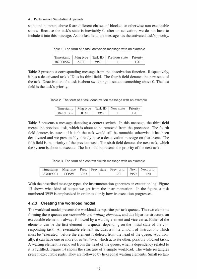
4. Performance Simulation Approach
state and numbers above 0 are different classes of blocked or otherwise non-executable
states. Because the task’s state is inevitably 0, after an activation, we do not have to
include it into this message. As the last field, the message has the activated task’s priority.
Table 1. The form of a task activation message with an example
Timestamp Msg type Task ID Previous state Priority
387000567 ACTI 3959 1 120
Table 2 presents a corresponding message from the deactivation function. Respectively,
it has a deactivated task’s ID as its third field. The fourth field denotes the new state of
the task. Deactivation of a task is about switching its state to something above 0. The last
field is the task’s priority.
Table 2. The form of a task deactivation message with an example
Timestamp Msg type Task ID New state Priority
387051332 DEAC 3959 1 120
Table 3 presents a message denoting a context switch. In this message, the third field
means the previous task, which is about to be removed from the processor. The fourth
field denotes its state – if it is 0, the task would still be runnable, otherwise it has been
deactivated and we presumably already have a deactivation message on that event. The
fifth field is the priority of the previous task. The sixth field denotes the next task, which
the system is about to execute. The last field represents the priority of the next task.
Table 3. The form of a context-switch message with an example
Timestamp Msg type Prev. Prev. state Prev. prio. Next Next prio.
387009901 COSW 3963 0 120 3959 120
With the described message types, the instrumentation generates an execution log. Figure
13 shows what kind of output we get from the instrumentation. In the figure, a task
numbered 3959 is emphasized in order to clarify how its execution progresses.
4.2.3 Creating the workload model
The workload model presents the workload as bipartite per-task queues. The two elements
forming these queues are executable and waiting elements, and due bipartite structure, an
executable element is always followed by a waiting element and vice versa. Either of the
elements can be the first element in a queue, depending on the initial state of the cor-
responding task. An executable element includes a finite amount of instructions which
must be “executed” before the element is deleted from the head of the queue. Addition-
ally, it can have one or more of activations, which activate other, possibly blocked tasks.
A waiting element is removed from the head of the queue, when a dependency related to
it is fulfilled. Figure 14 shows the structure of a simple workload. The white rectangles
present executable parts. They are followed by hexagonal waiting elements. Small rectan-
42
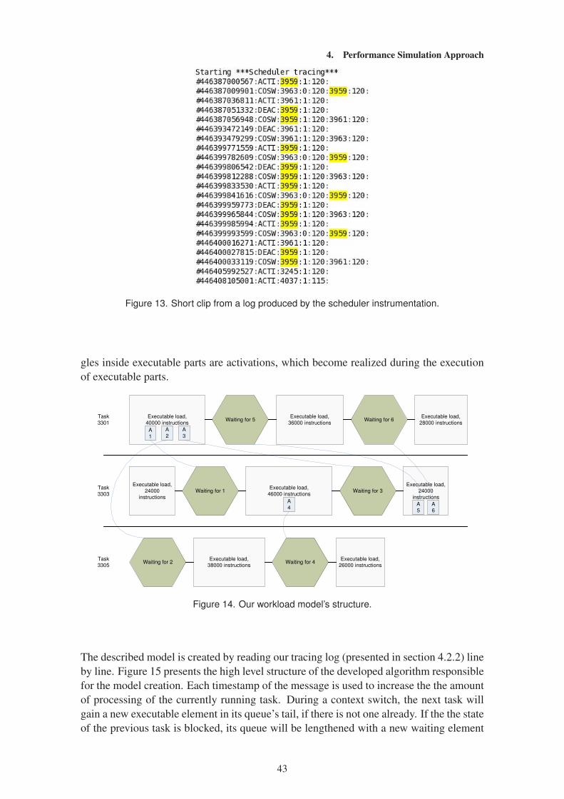
4. Performance Simulation Approach
Figure 13. Short clip from a log produced by the scheduler instrumentation.
gles inside executable parts are activations, which become realized during the execution
of executable parts.
Executable load,
40000 instructionsWaiting for 5
Executable load,
36000 instructionsWaiting for 6
Executable load,
28000 instructions
Executable load, 24000
instructions
Waiting for 1Executable load,
46000 instructions
Waiting for 2Executable load,
38000 instructionsWaiting for 4
Executable load, 26000 instructions
Waiting for 3Executable load,
24000
instructions
A
1
A
2
A
4
A
3
A
5
A
6
Task
3301
Task
3303
Task 3305
Figure 14. Our workload model’s structure.
The described model is created by reading our tracing log (presented in section 4.2.2) line
by line. Figure 15 presents the high level structure of the developed algorithm responsible
for the model creation. Each timestamp of the message is used to increase the the amount
of processing of the currently running task. During a context switch, the next task will
gain a new executable element in its queue’s tail, if there is not one already. If the the state
of the previous task is blocked, its queue will be lengthened with a new waiting element
43
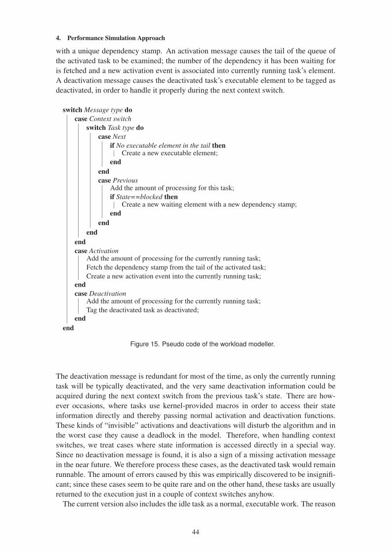
4. Performance Simulation Approach
with a unique dependency stamp. An activation message causes the tail of the queue of
the activated task to be examined; the number of the dependency it has been waiting for
is fetched and a new activation event is associated into currently running task’s element.
A deactivation message causes the deactivated task’s executable element to be tagged as
deactivated, in order to handle it properly during the next context switch.
switch Message type do
case Context switch
switch Task type do
case Next
if No executable element in the tail thenCreate a new executable element;
end
end
case PreviousAdd the amount of processing for this task;
if State==blocked thenCreate a new waiting element with a new dependency stamp;
end
end
end
end
case ActivationAdd the amount of processing for the currently running task;
Fetch the dependency stamp from the tail of the activated task;
Create a new activation event into the currently running task;
end
case DeactivationAdd the amount of processing for the currently running task;
Tag the deactivated task as deactivated;
end
end
Figure 15. Pseudo code of the workload modeller.
The deactivation message is redundant for most of the time, as only the currently running
task will be typically deactivated, and the very same deactivation information could be
acquired during the next context switch from the previous task’s state. There are how-
ever occasions, where tasks use kernel-provided macros in order to access their state
information directly and thereby passing normal activation and deactivation functions.
These kinds of “invisible” activations and deactivations will disturb the algorithm and in
the worst case they cause a deadlock in the model. Therefore, when handling context
switches, we treat cases where state information is accessed directly in a special way.
Since no deactivation message is found, it is also a sign of a missing activation message
in the near future. We therefore process these cases, as the deactivated task would remain
runnable. The amount of errors caused by this was empirically discovered to be insignifi-
cant; since these cases seem to be quite rare and on the other hand, these tasks are usually
returned to the execution just in a couple of context switches anyhow.
The current version also includes the idle task as a normal, executable work. The reason
44
4. Performance Simulation Approach
for this is that the idle can often represent the time when the system is waiting for user
interactions. The response times of the user must naturally also be taken into account
also in the simulated system, and the easiest way to ensure it is to let the processors also
execute the idle sections.
4.3 System modelling and simulation
In our case, the system modelling means the development of an abstract consumer for the
generated workload model. Obviously, the workload should also be consumed equally
such as with the real system, which we are trying to model. The abstraction level of the
simulator, for the actual execution part of the tasks, is very high – basically, we just per-
form a repetitive subtraction operation, at a speed defined by the simulated processors’
cycles-per-instruction value. The scheduling is modelled more accurately, and the depen-
dencies, presented in the workload model, are naturally strictly obeyed when the tasks are
executed.
The implemented performance simulator has some modularity, and therefore different
scheduling algorithms and system architecture alternatives should be easy to add after-
wards. The first system implemented and discussed in this work is a homogeneous ar-
chitecture with a centralized scheduler. This means that the processors use the scheduler
individually to fetch the next task, and the scheduling can only take place for one pro-
cessor at a time. Other processors will be forced to wait if there is a concurrent attempt
for scheduler access. This causes an extra overhead to the system, besides the normal
scheduling overhead. The main memory is also centralized and shared in the model (see
section 2.3.2), which eases the simulation as memory access times can be thought to be
same as in the original system. The simulator implements the finite state machine pre-
sented in figure 16.
The simulator is fed with the workload model (see section 4.2.3). First, the model is
checked to be deadlock-free, because a part of the workload will otherwise remain unex-
ecuted. The simulator begins by forming initial run and wait queues. Initially runnable
tasks of the workload model are naturally placed into the run queue, and non-runnable
tasks respectively into the wait queue. The processors are modelled in dedicated threads,
which are synchronously proceeding simulation steps. The simulation step is freely ad-
justable, beginning from one clock cycle. The first actual state after the initial prepara-
tions is the idle state. However, a flag denoting a need for rescheduling is initially up and
each processor therefore calls the scheduler. One of the processors manages to access
the scheduler, whilst others are forced to wait. Waiting for the scheduler is modelled as
a dedicated state in the state machine. As previously mentioned, this is one factor that
lowers the efficiency of systems with a centralized scheduler, as the processors are unable
to do useful work, while they are waiting for the scheduler. After successful access to the
scheduler, either by waiting for or accessing it directly, the simulation models the schedul-
ing overhead, which presents the overhead related to the scheduling procedures. Selecting
the next task from a group of several tasks causes some extra computation. Additionally,
scheduling is usually followed by a context switch, which means transferring the data
of the next task to the processor. This also causes some overhead, but in our case, the
measured workload already includes both the scheduling and context switching overhead.
The amount of the overhead can be set to represent an estimate of the additional overhead
caused by the multi-processor scheduling. As already said, queuing the scheduler access
is taken into account in this simulation and it does not need to be approximated in the
45

4. Performance Simulation Approach
Idle
Scheduling overheadWaiting for scheduler
Processing a task
Reschedule /Scheduler free
Reschedule /Scheduler busy
Scheduler free
Reschedule || End of timeslice || End of task /
Scheduler busy
Reschedule || End of timeslice || End of task /
Scheduler free
Overhead done
No task available
Overhead done &&
Reschedule
Figure 16. A finite state machine, with rather few states, is used to simulate a homogeneous
architecture with a centralized scheduler.
scheduling overhead.
In the worst case, a context switch may require a reloading of the whole cache memory.
This situation is called a cold cache. A cold cache is the consequence of a “new” task’s
scheduling to a processor: its cache is occupied by the previous task’s data and the cache
must be thereby cleared and then loaded with the proper data. This means that the tasks
should be kept running within the same processor as much as possible. If the cache has
the correct data ready for a task, the cache is respectively called a hot cache. Multi-
processor scheduling algorithms can utilize knowledge on the tasks’ previously allocated
processors and thereby, they can attempt to avoid movement of the tasks between different
processors. The implemented algorithm in the simulator did not include this kind of
feature, as the measured workload also includes the cache overhead from the original
system.
After the scheduling overhead has been consumed, the next state is usually the actual
execution of a task, in a state called as processing a task. The only exceptions to this are
the cases when a rescheduling flag has been raised during the scheduling overhead con-
sumption, which causes the processor to schedule again, or that there is no task available
to the processor, which causes it to enter the idle state. Without an immediate reschedul-
ing, the simulation begins to execute the scheduled task. Depending on the set CPI value,
one instruction usually takes more than one, for example 1.5 cycles to complete. As with
the workload modelling, we do not use an exact instruction-specific CPI value but an es-
timated average of it. During the execution of tasks, the dependencies presented in the
workload model become fulfilled. The fulfilment triggers the following operations in the
simulator: an update in a dependency matrix, a migration of corresponding tasks from
the wait queue to the run queue and a possible rescheduling. The dependency matrix is
46

4. Performance Simulation Approach
used for tracking fulfilled dependencies – a waiting point in the workload model can be
simply skipped if the required dependency is already filled in the simulated run. The task
execution continues until a need for reschedule flag is raised, the task uses its entire time
slice or the runnable part of the task is consumed totally. All of these cause the proces-
sor to schedule, and depending on the scheduler’s availability, the next possible states are
waiting the scheduler or processing the scheduler overhead.
The implemented scheduling algorithm has a centralized run-queue, which furthermore
consists of separate round-robin (see section 3.3) sub-queues for each priority. In gen-
eral terms, this algorithm is a simplified and centralized version of the algorithm of the
previous Linux versions (see section 4.2.1). Because the highest priority process with the
longest waiting time is always selected, and on the other hand a rescheduling occurs every
time tasks are activated, the algorithm assures that N runnable processes with the high-
est priorities are always executing in a system with N processors. When looking more
closely at the simulators internal functionality, in addition to the task itself, the scheduler
also returns the scheduling overhead and time slice values, as shown in figure 17. As
this type of per-priority run queue scheduler has a virtually constant overhead, and the
workload model itself includes a scheduling overhead from the original system, we did
not develop any kind of approximation function for the scheduling overhead. Instead,
the used scheduler returns a small constant amount of cycles. Of course, the overhead
could be also accurately modelled based on the actual computation needed in picking the
next task. In the current version, the given time slice is also modelled in a coarse way:
it varies stochastically between the values that we observed with measurements from the
real-world system. The real operating systems calculate this value premising on charac-
teristics of the task, such as the load of the system.
Scheduling overhead Time slice
The task’s event queue
Figure 17. The scheduler returns a structure, which consists of the whole task event queue,
scheduling overhead and time slice values.
4.4 Analysis with visualization
A 3D-visualization tool called PerVisGL, originally created by Yrjönen [7], was extended
during this work to support multiple data logs, in order to visualize multi-processor sys-
tems. In addition, we also developed other minor features for it, mostly related to easier
47
4. Performance Simulation Approach
task identification. PerVisGL allows the use of three-dimensional space freely, to repre-
sent arbitrary data after a data-specific reader has been developed. In this case, we selected
adjacent 100 x 10 x 10 rectangular boxes to present the execution. Each of the described
boxes denotes one processor. The longest dimension is aligned with the x-axis and is 100
units. This denotes the time, and despite of the actual duration of the log, the whole log
is scaled to this interval. The y-axis, up to 10 units, denotes the relative load of the CPU
in a linear fashion. The z-axis, up to 10 units as well, is relative to the priorities of the
tasks, but not linearly. Normal non-real-time tasks use a scale from 0 to 8 units, real-time
tasks use the next distance from 8 to 9 units and so called background load, which is the
scheduling overhead, is the longest in the z-direction, reaching a full 10 units. Thus, the
“thickness” of the graph presents the importance of the work; the background load may
not be esteemed, but it is obligatory and at least important to notify.
We also use colours as an additional dimension. Tasks can be identified by their colours;
the colour value for a task is calculated from its task number. The function, calculating
this value, uses a simple hash method in order to clearly present different colours for
consecutive task numbers. One can also give desired task numbers, which will be the
only ones to be coloured. This notably emphasizes the graph, when there are dozens or
hundreds of tasks presented simultaneously.
Instead of drawing the tasks strictly in a sequential order along the time-axis, the ap-
plication splits the space into smaller blocks. This is due to the overwhelming amount of
context switches present in a typical log; the graph would be as hard to read as the orig-
inal, raw text-form log itself. For example, if we want to present our data in ten blocks,
the first block represents the distribution of computation in the first tenth of the log, and
its dimensions are 10 x 10 x 10 respectively. The boxes presenting individual tasks are
drawn in this space, one upon the other. Tasks with the highest priorities go to the bottom,
because they were also the thickest ones. The block now fills the x-axis for one tenth of
the total distance, but the y- and the z-axes have varying sizes in different positions. The
height of a box presents the corresponding task’s share of computation during the block
interval, and because the boxes are piled vertically, the top of the topmost box also shows
the total relative computation. Any free space over the topmost box correspondingly rep-
resents the amount of idle. The z-dimension is also task-wise and represents the priority,
as already mentioned in this section.
Figure 18 is used here as a practical example of the functionality of the visualization.
The figure has roughly ten blocks visible. In the very first block, three different tasks,
drawn in blue, red and orange, have been executed, and all of them have different prior-
ities. “The orange task” had the highest priority and therefore it is drawn at the bottom
with the thickest box. Furthermore, these three tasks, together, used roughly 55 percent of
the available CPU time during this block’s interval, since there are 4.5 units of free space
at the top in the y-axis. In the next blocks, only red and blue tasks have been running, and
finally in the last blocks visible, there is only a green task running.
Figure 18 also shows how the visualization tool draws grids to help in the determining
of load and priority values. The distance between two grid lines is one unit, so in the
direction of the y-axis, the lines correspond to a change of 10 % in the load of the system.
In the direction of the x-axis, the scale is not linear since most of it, the values from 0 to
8 units, were defined for non-real-time tasks as we are usually more interested of them.
Non-real-time tasks in Linux have only 40 priorities against the 100 priorities of real-time
tasks [27, p. 265].
48

4. Performance Simulation Approach
Figure 18. A simple visualization to clarify the visualization applications functionality.
The interface between the simulator and the visualization tool is a set of log files: one
file per simulated processor. One line in a log represents a set time interval, however
a context switch, always triggers the logging so that data on each task’s execution is
acquired properly. Each line has a time stamp, the amount of overhead in the interval, the
amount of the actual processing in the interval, a task number and a priority. Because the
time stamp in the log file is in processor cycles, the simulated device’s clock rate must be
entered into the visualization tool, in order to present the correct “wall clock” time values
in the graph.
49

5. ResultsThis chapter presents the results achieved during the work. Firstly, the performed valida-
tions are discussed and then we will analyze the whole method.
5.1 Validation of the models
As explained in section 3.6 the simulation models can be hard to validate completely.
In this work, two somewhat different validation methods were applied. The first one was
more coarse and meant for early phase testing, whereas the second one gives useful results
about the accuracy and feasibility of the approach.
The first validation was performed with a simple self-made application, which runs a se-
lected amount of threads using an inter-thread synchronization mechanism. We will mea-
sure the execution of this application, model it and finally simulate the acquired workload
with different multi-processor systems. As the internal functionality of the application is
known, it is possible to see if our performance simulation method gives too optimistic or
too pessimistic results for the given workload.
The second validation method is more general and clearly more challenging. The work-
load was measured from a dual-core PC with operating system which was forced to use
only one core. The measured workload is then simulated in modelled dual-processor ar-
chitecture and the simulation results are compared to a run of the same tasks in a PC
which is using the both cores. The modelled and real-world systems should now be effec-
tively the same. The result of this is that the difference in the results directly presents the
accuracy of the whole method.
In other words, we are validating the workload model, the simulation model and the
whole method at the same time.
5.1.1 Threads with barrier synchronization
The self-made application for this validation purpose performed repetitive memory op-
erations with three child threads. These child threads each had 250 iterations and the
iterations were synchronized with the so called barrier synchronization, which holds the
threads in a barrier point, until they have all reached it. In our case, with three threads,
the first and second threads to reach the barrier are blocked temporarily. The third thread
continues its execution directly without blocking at the barrier, and this event also releases
the two other ones to continue.
This test case was selected to be inconvenient for our method. Since, one of the threads
in every iteration proceeds without blocking, the method will not see that dependency
at all, although there clearly is one by knowing the test application’s internal structure.
Thereby, the method could produce results that are too optimistic. However, in the long
run, the threads will encounter an equal amount of blocking when compared to each other,
and therefore they are still clearly synchronized with each other, although one dependency
per iteration is missed. This means that the method should be able to also simulate the
execution in a roughly synchronized way.
Figure 19 presents the visualization of the trace achieved from the described test appli-
cation. Only the threads affiliated to the test application, one parent, number 11786, and
three child threads, numbers 11787, 11788 and 11789, are coloured. Particularly in the
middle part, the three child threads can be seen to execute quite equally.
Table 4 presents the original trace and the results for four different simulated platforms.
The amount of total execution is given in millions of CPU cycles, and the relative perfor-
50
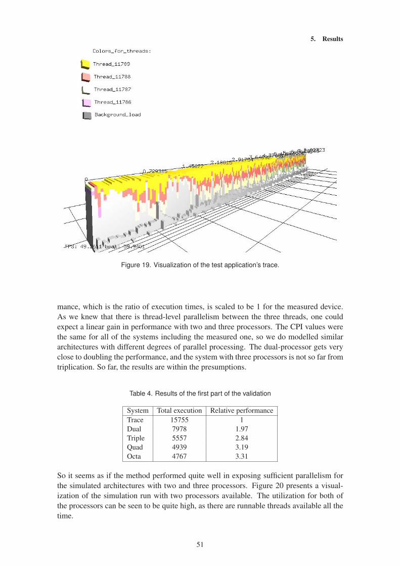
5. Results
Figure 19. Visualization of the test application’s trace.
mance, which is the ratio of execution times, is scaled to be 1 for the measured device.
As we knew that there is thread-level parallelism between the three threads, one could
expect a linear gain in performance with two and three processors. The CPI values were
the same for all of the systems including the measured one, so we do modelled similar
architectures with different degrees of parallel processing. The dual-processor gets very
close to doubling the performance, and the system with three processors is not so far from
triplication. So far, the results are within the presumptions.
Table 4. Results of the first part of the validation
System Total execution Relative performance
Trace 15755 1
Dual 7978 1.97
Triple 5557 2.84
Quad 4939 3.19
Octa 4767 3.31
So it seems as if the method performed quite well in exposing sufficient parallelism for
the simulated architectures with two and three processors. Figure 20 presents a visual-
ization of the simulation run with two processors available. The utilization for both of
the processors can be seen to be quite high, as there are runnable threads available all the
time.
51

5. Results
Figure 20. The visualization of the test application run in a simulated dual-processor system.
In figure 21, the test application is simulated to use three processors. The workload man-
ages to keep all the available processors relatively busy, which is still reasonable since we
know that the three threads should be able to run concurrently.
Figure 21. The visualization of the test application run in a simulated triple-processor system.
When we add one more processor to the system, we should not get a significant perfor-
mance gain, because there is not enough parallelism available. The small exceeding of
the relative performance of 3 with four processors can be explained with other small tasks
present in the workload. In figure 22, we can see how the execution is divided among four
processing units. The graphical analysis also confirms that there are idle slots clearly vis-
ible, and the utilization of the system is not the best possible. Figure 23 demonstrates the
scalability of the simulation also in addition to the visualization. The simulated system
has eight processors and therefore it could be a type of super-computer. The figure clearly
shows that the amount of parallelism in the workload was not sufficient for this kind of
52
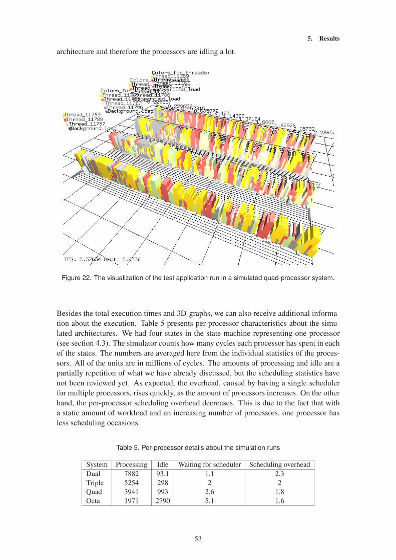
5. Results
architecture and therefore the processors are idling a lot.
Figure 22. The visualization of the test application run in a simulated quad-processor system.
Besides the total execution times and 3D-graphs, we can also receive additional informa-
tion about the execution. Table 5 presents per-processor characteristics about the simu-
lated architectures. We had four states in the state machine representing one processor
(see section 4.3). The simulator counts how many cycles each processor has spent in each
of the states. The numbers are averaged here from the individual statistics of the proces-
sors. All of the units are in millions of cycles. The amounts of processing and idle are a
partially repetition of what we have already discussed, but the scheduling statistics have
not been reviewed yet. As expected, the overhead, caused by having a single scheduler
for multiple processors, rises quickly, as the amount of processors increases. On the other
hand, the per-processor scheduling overhead decreases. This is due to the fact that with
a static amount of workload and an increasing number of processors, one processor has
less scheduling occasions.
Table 5. Per-processor details about the simulation runs
System Processing Idle Waiting for scheduler Scheduling overhead
Dual 7882 93.1 1.1 2.3
Triple 5254 298 2 2
Quad 3941 993 2.6 1.8
Octa 1971 2790 5.1 1.6
53

5. Results
Figure 23. The visualization of the test application run in a simulated super-computer, which has
eight processors in total.
5.1.2 Threaded video encoding
The selected application for the second part of the validation was FFmpeg [43], which is
a multi-threaded video encoding software for Linux. Normally the application selects a
suitable amount of threads to use depending on the hardware, naturally one thread per one
processor, but in this case, it was forced to use two threads for encoding. In addition to the
two threads performing the encoding, the application’s “main thread” is also running and
probably performing some kind of control tasks, but it does not utilize the CPU as heavily
as the two other threads. The encoder’s threads also have a lot of dependencies between
them; threads are almost always blocked when they are switched from the execution. This
is a good situation for our validation purposes. For example, a threaded file compression
was initially planned as a validation case, but its threads were noticed to remain runnable
when they were switched out. Due to this fact, the validation would have been too trivial,
as the dependencies and their fulfilments would only have had a small effect.
The operating system was Fedora Core 8 Linux with a self-built kernel version 2.6.24.3.
Self-building of the kernel was required due to the SystemTap instrumentation. The op-
erating system was forced to use only one of the two cores provided by the Core 2 Duo
workstation, running at 2.16 GHz. The test case was to encode a motion JPEG AVI file
into a DVD PAL MPEG-2 format. The size of the original file was 10.0 megabytes and
the output file enlarged to 23.7 megabytes. This encoding process was measured and then
fed into the combination of the workload modeller and simulator. Figure 24 shows that
there were also plenty of other tasks involved. However, most of the processing was done
by the three threads of the video encoder.
The video encoding was also executed in the described workstation with both cores in
54
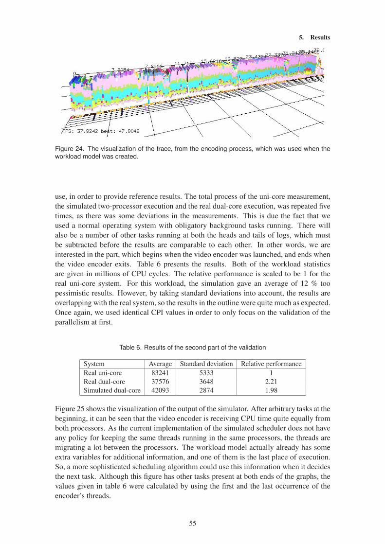
5. Results
Figure 24. The visualization of the trace, from the encoding process, which was used when the
workload model was created.
use, in order to provide reference results. The total process of the uni-core measurement,
the simulated two-processor execution and the real dual-core execution, was repeated five
times, as there was some deviations in the measurements. This is due the fact that we
used a normal operating system with obligatory background tasks running. There will
also be a number of other tasks running at both the heads and tails of logs, which must
be subtracted before the results are comparable to each other. In other words, we are
interested in the part, which begins when the video encoder was launched, and ends when
the video encoder exits. Table 6 presents the results. Both of the workload statistics
are given in millions of CPU cycles. The relative performance is scaled to be 1 for the
real uni-core system. For this workload, the simulation gave an average of 12 % too
pessimistic results. However, by taking standard deviations into account, the results are
overlapping with the real system, so the results in the outline were quite much as expected.
Once again, we used identical CPI values in order to only focus on the validation of the
parallelism at first.
Table 6. Results of the second part of the validation
System Average Standard deviation Relative performance
Real uni-core 83241 5333 1
Real dual-core 37576 3648 2.21
Simulated dual-core 42093 2874 1.98
Figure 25 shows the visualization of the output of the simulator. After arbitrary tasks at the
beginning, it can be seen that the video encoder is receiving CPU time quite equally from
both processors. As the current implementation of the simulated scheduler does not have
any policy for keeping the same threads running in the same processors, the threads are
migrating a lot between the processors. The workload model actually already has some
extra variables for additional information, and one of them is the last place of execution.
So, a more sophisticated scheduling algorithm could use this information when it decides
the next task. Although this figure has other tasks present at both ends of the graphs, the
values given in table 6 were calculated by using the first and the last occurrence of the
encoder’s threads.
55

5. Results
Figure 25. The visualization of the encoding simulation results with all the tasks shown equally.
Figure 26 has only the encoder’s threads emphasized, for easier understanding. This
figure also shows that, in the beginning, there is a group of other tasks causing the load
to the system. After that, the visualization reveals that the encoding process is able to
roughly utilize 90 % of the available processing power in our simulated two-processor
architecture. This type of information can be a very useful to a system designer, and on the
other hand, obtaining the value from raw text-form logs would probably be troublesome
or inconvenient. In addition to this broad overview, the visualization also shows more
detailed statistics. For example, some higher priority processes, longer in the Z-direction
and drawn with black and grey, are also occasionally receiving small partitions of the
CPU time.
Figure 26. The visualization of the encoding simulation results, where only the threads belonging
to the encoding task are emphasized.
56
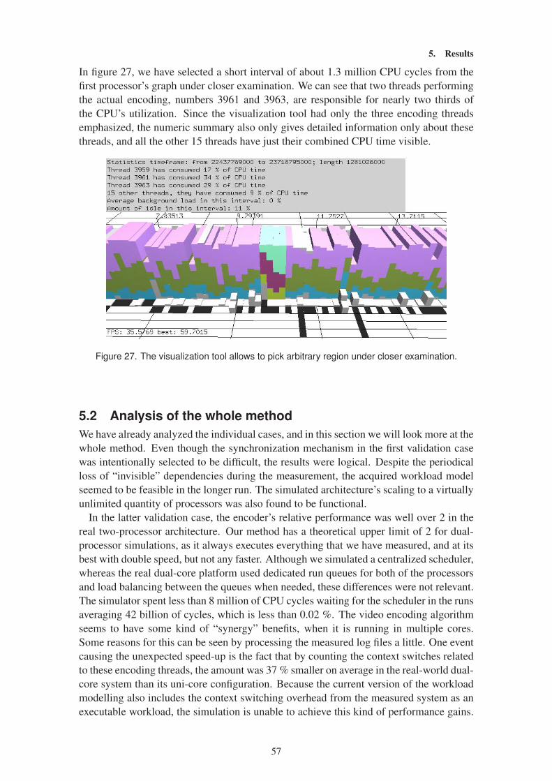
5. Results
In figure 27, we have selected a short interval of about 1.3 million CPU cycles from the
first processor’s graph under closer examination. We can see that two threads performing
the actual encoding, numbers 3961 and 3963, are responsible for nearly two thirds of
the CPU’s utilization. Since the visualization tool had only the three encoding threads
emphasized, the numeric summary also only gives detailed information only about these
threads, and all the other 15 threads have just their combined CPU time visible.
Figure 27. The visualization tool allows to pick arbitrary region under closer examination.
5.2 Analysis of the whole method
We have already analyzed the individual cases, and in this section we will look more at the
whole method. Even though the synchronization mechanism in the first validation case
was intentionally selected to be difficult, the results were logical. Despite the periodical
loss of “invisible” dependencies during the measurement, the acquired workload model
seemed to be feasible in the longer run. The simulated architecture’s scaling to a virtually
unlimited quantity of processors was also found to be functional.
In the latter validation case, the encoder’s relative performance was well over 2 in the
real two-processor architecture. Our method has a theoretical upper limit of 2 for dual-
processor simulations, as it always executes everything that we have measured, and at its
best with double speed, but not any faster. Although we simulated a centralized scheduler,
whereas the real dual-core platform used dedicated run queues for both of the processors
and load balancing between the queues when needed, these differences were not relevant.
The simulator spent less than 8 million of CPU cycles waiting for the scheduler in the runs
averaging 42 billion of cycles, which is less than 0.02 %. The video encoding algorithm
seems to have some kind of “synergy” benefits, when it is running in multiple cores.
Some reasons for this can be seen by processing the measured log files a little. One event
causing the unexpected speed-up is the fact that by counting the context switches related
to these encoding threads, the amount was 37 % smaller on average in the real-world dual-
core system than its uni-core configuration. Because the current version of the workload
modelling also includes the context switching overhead from the measured system as an
executable workload, the simulation is unable to achieve this kind of performance gains.
57
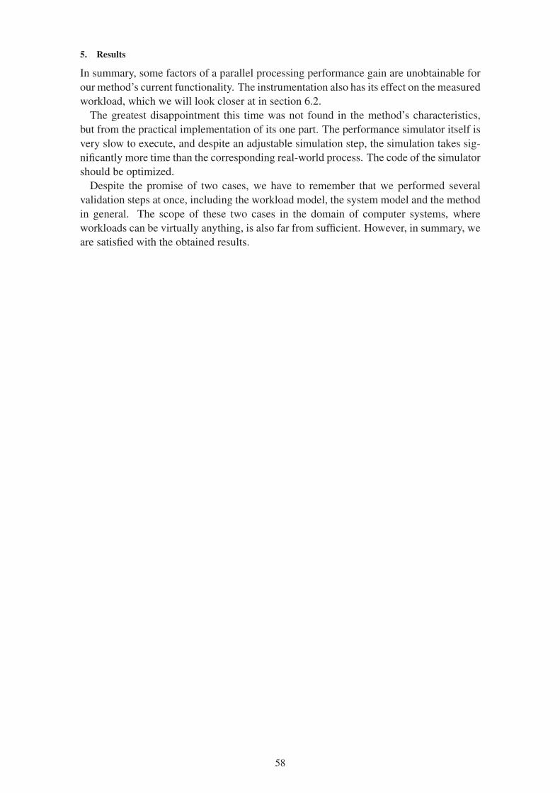
5. Results
In summary, some factors of a parallel processing performance gain are unobtainable for
our method’s current functionality. The instrumentation also has its effect on the measured
workload, which we will look closer at in section 6.2.
The greatest disappointment this time was not found in the method’s characteristics,
but from the practical implementation of its one part. The performance simulator itself is
very slow to execute, and despite an adjustable simulation step, the simulation takes sig-
nificantly more time than the corresponding real-world process. The code of the simulator
should be optimized.
Despite the promise of two cases, we have to remember that we performed several
validation steps at once, including the workload model, the system model and the method
in general. The scope of these two cases in the domain of computer systems, where
workloads can be virtually anything, is also far from sufficient. However, in summary, we
are satisfied with the obtained results.
58

6. DiscussionWe will review here the strengths and weaknesses of the method. As the work was just
the first phase of a larger work, we will also cover some possible future scenarios.
6.1 Advantages of the method
This section presents the aspects that we found particularly successful during the work.
We will look first at the subtopics and then discuss the whole method.
The instrumentation provides an easy completion of measurements, since we only need
information from three different points of an operating system: task activations, task de-
activations and context switches. If the states of the tasks can be reliably checked during
the context switches, a previous task can be found out to be deactivated from the con-
text switch’s probing point. Probing the deactivations becomes effectively redundant and
thereby only two points of the operating system must be instrumented. The instrumen-
tation’s functionality is also simple and needs only a few lines of additional code. Due
to these facts, all operating systems, implementing somewhat the same kind of central-
ized active and blocked task handling, should be possible to instrument with the given
guidelines.
The workload modelling step is automated and does not require user interaction, ex-
cluding possible CPI value settings. When compared to some other methods, the user
does not need to be familiar with the workload in detail.
Due to the simulation’s accurate modelling of the scheduling, it could be used in a uni-
processor domain as well – in addition to parallel processing, one could test uni-processor
scheduling algorithms. As the simulator uses workloads which are measured from real-
world devices, the algorithms would be under realistic testing.
Our visualization approach is commonly thought to be easy to understand. It can handle
varying amounts of data and visualize them in an equally understandable way. Empha-
sizing the desired parts of the execution, and giving statistics on the selected areas were
noticed to be useful resources.
Despite the whole method’s high level of abstraction, the cases selected for validation at
least gave reasonable and comparatively accurate results. The autonomous processing of
measurements from real-world devices, and their linkage into simulated domains was also
found to be a working solution. This removes the demand for manual workload creation
present in several other methods. The most important breakthrough during the work was
the exploration of parallelism and dependencies by instrumenting the scheduling queues.
This idea also proved to be feasible and relatively straightforward to implement.
6.2 Considerations of the method
We already had knowledge of some of the method’s restrictions at the beginning of the
work, and we also encountered some new ones during the work. This section declares
these aspects. Once again, we will first look at the individual areas and then the complete
method.
Despite the small code size of the instrumentation, we are probing a very sensitive
part of an operating system. The target events are also recurring very frequently. This
causes an unavoidable probing effect, which makes the workloads to seem larger than
they really are. Equally, the measured system seems to be slower, which also affects the
simulated system. Table 7 presents statistics on five test runs, where the video encoding
task from the second validation case was run with and without instrumentation, in order
59
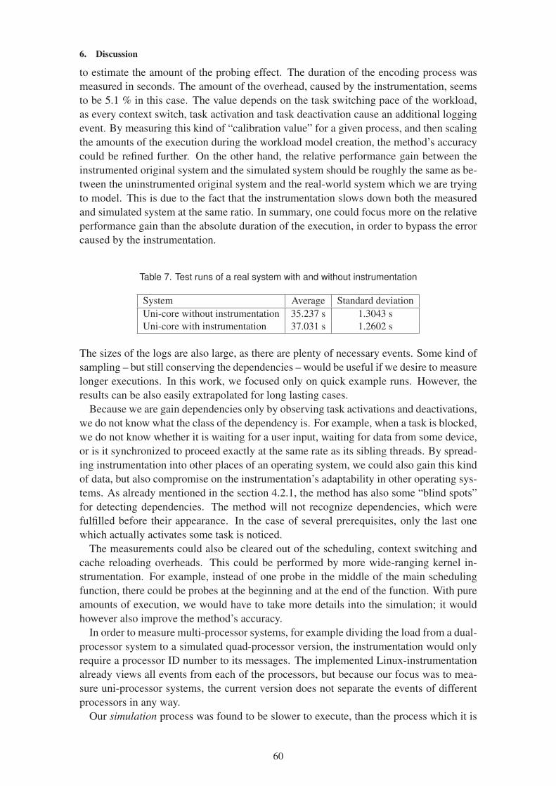
6. Discussion
to estimate the amount of the probing effect. The duration of the encoding process was
measured in seconds. The amount of the overhead, caused by the instrumentation, seems
to be 5.1 % in this case. The value depends on the task switching pace of the workload,
as every context switch, task activation and task deactivation cause an additional logging
event. By measuring this kind of “calibration value” for a given process, and then scaling
the amounts of the execution during the workload model creation, the method’s accuracy
could be refined further. On the other hand, the relative performance gain between the
instrumented original system and the simulated system should be roughly the same as be-
tween the uninstrumented original system and the real-world system which we are trying
to model. This is due to the fact that the instrumentation slows down both the measured
and simulated system at the same ratio. In summary, one could focus more on the relative
performance gain than the absolute duration of the execution, in order to bypass the error
caused by the instrumentation.
Table 7. Test runs of a real system with and without instrumentation
System Average Standard deviation
Uni-core without instrumentation 35.237 s 1.3043 s
Uni-core with instrumentation 37.031 s 1.2602 s
The sizes of the logs are also large, as there are plenty of necessary events. Some kind of
sampling – but still conserving the dependencies – would be useful if we desire to measure
longer executions. In this work, we focused only on quick example runs. However, the
results can be also easily extrapolated for long lasting cases.
Because we are gain dependencies only by observing task activations and deactivations,
we do not know what the class of the dependency is. For example, when a task is blocked,
we do not know whether it is waiting for a user input, waiting for data from some device,
or is it synchronized to proceed exactly at the same rate as its sibling threads. By spread-
ing instrumentation into other places of an operating system, we could also gain this kind
of data, but also compromise on the instrumentation’s adaptability in other operating sys-
tems. As already mentioned in the section 4.2.1, the method has also some “blind spots”
for detecting dependencies. The method will not recognize dependencies, which were
fulfilled before their appearance. In the case of several prerequisites, only the last one
which actually activates some task is noticed.
The measurements could also be cleared out of the scheduling, context switching and
cache reloading overheads. This could be performed by more wide-ranging kernel in-
strumentation. For example, instead of one probe in the middle of the main scheduling
function, there could be probes at the beginning and at the end of the function. With pure
amounts of execution, we would have to take more details into the simulation; it would
however also improve the method’s accuracy.
In order to measure multi-processor systems, for example dividing the load from a dual-
processor system to a simulated quad-processor version, the instrumentation would only
require a processor ID number to its messages. The implemented Linux-instrumentation
already views all events from each of the processors, but because our focus was to mea-
sure uni-processor systems, the current version does not separate the events of different
processors in any way.
Our simulation process was found to be slower to execute, than the process which it is
60

6. Discussion
mimicking. Simulation studies are typically performed in accelerated time for systems,
whose internal working does not need to be known in a very detailed way [5, p. 77]. This
would be advantageous for us, in order to flexibly examine several possible architectures,
however the current implementation does not provide this kind of quickness. For example,
the encoding tasks presented in section 5.1.2 were under 40 and 20 seconds when executed
in uni- and dual-core systems. The duration of the simulation run for this workload was
nearly 60 minutes. The utilization of rather heavy-weighted data structures such as C++
vectors and maps in the workload models, as well as in the run and waiting queues is
probably the main reason for the slowness.
The visualization application does not give any kind of information on dependencies at
its present state. This kind of extension is easy to implement at a code level, however,
finding a practical and understandable graphical form is more difficult.
Because the method is seeking thread-level parallelism (see section 3.1) among the al-
ready existing threads, we do not gain much new information out of the workloads which
are not using threads. However, the method will find out the independent processes and
allocate them to different processors when appropriate, but that is an assignment which
could be essentially completed by using just common sense, instead of any kind of sim-
ulations. For example, we can say that executions of a word processor and an Internet
browser – two clearly uncorrelated applications – could be successfully allocated to dif-
ferent processors in order to get a performance gain. In addition, some multi-threaded
applications are adaptive enough to execute only a single thread in a single processor sys-
tem, which would obviously harm measurements in our method. The method does not try
to find parallelism inside applications written sequentially.
6.3 Future work
During this work, we only focused on the homogeneous systems. A simulation of hetero-
geneous systems would be technically a lightweight update. On the other hand, knowl-
edge on the workload’s parts, which could be executed in non-general-purpose processors,
is hard to automate. Another difficulty is to approximate the amount of the scaled work-
load in such processors. One possible way would be to manually seek for tasks executing
some algorithms, which are known to be feasible to implement with more hardware-
oriented solutions. The ID numbers of these tasks would then be fed to the simulator
with a configuration file. The scheduler would give these tasks only to co-processors,
when they are runnable. Another possible approach would require more details on the
workload model. The next detail level could be a representation of work with very basic
operations, such as memory reads, memory writes and executions [36]. With characteris-
tics modelled for these operations per each computational unit, the heterogeneous system
would be able to consume the workload in a proper way.
61
7. ConclusionThis thesis presented a novel method for exposing thread-level parallelism from an ex-
isting device’s workload and simulating its execution in a multi-processor environment.
The work confirmed that the original, high-level idea of a modelling load from existing
devices to new, more parallel architectures is doable.
We also presented a validation of the method with two practical cases: the first case with
an “ad-hoc” test application and the second one with a more common video encoding
process. According to the case studies, the approach seems to be valid. The achieved
estimation of the method’s inaccuracy was from 10 to 15 %. On the other hand, more
wide-ranging validation cases will be still required before the true characteristics of the
method are known.
The method supports system designers in the early phases of the system design flow,
when the required amount of co-processing for the new system is being decided. The
most important contributions provided by this work are:
• An automatic generation of workload models from measurements
• Finding parallelism from a few simple locations of an operating system
• Highly abstracted simulation models
• Easily understandable visualizations of multi-processor systems’ load.
As our method has the automated workload generation, the amount of required work is
small when compared to several, more detailed simulation solutions. The results are still
useful, especially if the alternative is just an educated guess about the designed system’s
performance. The method however does not give support for analysing a single proces-
sor’s internal architecture changes.
The method exposes parallelism at the level of an operating system, and therefore does
not require a detailed knowledge on the workload’s internal structure. Our method pro-
vides support for many kinds of workloads without modifications, although the most ob-
vious way would be to attempt to find parallelism directly from the applications and algo-
rithms running on the measured system – and thereby lose the versatility. The restriction
is that the workload must be a threaded one. The generalization of the method for other
source systems is good, because the required instrumentation was kept intentionally as
minimal as possible. This is naturally aiding adaptability to other operating systems.
The high level of abstraction with the models mimicking the systems under design also
provides easiness for the system designers. The method’s scalability for a wide range of
number of parallel processors in the simulated system was found to be reasonable. The
extension of the method for heterogeneous system support was also discussed and seems
doable.
The method also provides support for the analysis of results, as our 3D-visualizations
were proved to be more informative than typical raw data logs. The designer can have a
quick overview of the distribution of the load in the system at a glance, whereas it would
not be possible with unprocessed text-form data.
62
References[1] Takalo J., Kääriäinen J., Parviainen P. & Ihme T. (2008) Challenges of software-
hardware co-design. prestudy in twins project. Tech. rep., VTT. URL: http://
www.vtt.fi/inf/pdf/workingpapers/2008/W91.pdf.
[2] Sommerville I. & Sawyer P. (1997) Requirements Engineering: A good practice
guide. Wiley, Chichester, England. 404 p.
[3] Nixon B.A. (1998) Managing performance requirements for information systems.
In: WOSP ’98: Proceedings of the 1st international workshop on Software and
performance, ACM Press, New York, NY, USA. Pp. 131–144.
[4] Berger A. (2002) Embedded Systems Design: An Introduction to Processes, Tools
& Techniques. CMP Books, Lawrence, USA. 237 p.
[5] Law A.M. (2006) Simulation Modeling and Analysis. McGraw-Hill Publishing Co.,
Europe. 800 p.
[6] Carson J.S. (2005) Introduction to modeling and simulation. In: WSC ’05: Proceed-
ings of the 37th conference on Winter simulation, Winter Simulation Conference.
Pp. 16–23., pp. 16–23.
[7] Yrjönen A. (2007) Performance analysis of software run-time behaviour using 3-D
visualization. Master’s thesis, Lappeenranta University of Technology, Department
of Information Technology, Lappeenranta.
[8] Bock P. (2001) Getting it Right: R&D Methods for Science and Engineering. Aca-
demic Press, San Diego, USA. 350 p.
[9] Hennesy J.L. & Patterson D.A. (2003) Computer Architecture: A Quantitative Ap-
proach. Morgan Kaufmann, San Francisco, USA. 1136 p.
[10] Flynn M.J. (1966) Very high-speed computing systems. Proceedings of the IEEE
vol. 54. Pp. 1901–1909.
[11] Hauser J.R. & Wawrzynek J. (1997) Garp: a MIPS processor with a reconfigurable
coprocessor. In: FPGAs for Custom Computing Machines, 1997. Proceedings., The
5th Annual IEEE Symposium on, Napa Valley, CA, USA. Pp. 12–21.
[12] Sriram S. & Bhattacharyya S.S. (2000) Embedded multiprocessors: Scheduling and
Synchronization. Marcel Dekker, Inc., New York, USA. 352 p.
[13] Gschwind M. (2006) The cell broadband engine: Exploiting multiple levels of par-
allelism in a chip multiprocessor. Tech. rep., IBM Research Division. URL: http:
//domino.research.ibm.com/library/cyberdig.nsf/papers/
1B2480A9DBF5B9538525723D0051A8C1/$File/rc24128.pdf.
[14] Stokes J. (2006) Inside the Machine: An Illustrated Introduction to Microprocessors
and Computer Architecture. No Starch Press, San Francisco, USA. 320 p.
[15] Rosch W.L. (1999) The Winn L. Rosch Hardware Bible. Que Publishing, USA. 1416
p.
63

[16] Ifeachor E.C. & Jervis B.W. (2002) Digital Signal Processing, A Practical Approach.
Pearson Education Limited, Harlow, England. 933 p.
[17] Maurer W.D. (2005) The effect of the harvard architecture on the teaching of assem-
bly language. J. Comput. Small Coll. 20, pp. 79–90.
[18] Zuchowski P.S., Reynolds C.B., Grupp R.J., Davis S.G., Cremen B. & Troxel B.
(2002) A hybrid asic and fpga architecture. In: ICCAD ’02: Proceedings of the
2002 IEEE/ACM international conference on Computer-aided design, ACM Press,
New York, NY, USA. Pp. 187–194.
[19] Tredennick N. & Shimamoto B. (2003) Go reconfigure [programmable logic in
handheld devices]. IEEE Spectrum 40, pp. 36–40.
[20] Verkest D. (2003) Machine chameleon [handheld devices]. IEEE Spectrum 40, pp.
41–46.
[21] Mukherjee S.S., Adve S.V., Austin T., Emer J. & Magnusson P.S. (2002) Perfor-
mance simulation tools. Computer 35, pp. 38–39.
[22] Hughes C.J., Pai V.S., Ranganathan P. & Adve S.V. (2002) Rsim: simulating shared-
memory multiprocessors with ILP processors. Computer 35, pp. 40–49.
[23] Magnusson P.S., Christensson M., Eskilson J., Forsgren D., Hallberg G., Hogberg
J., Larsson F., Moestedt A. & Werner B. (2002) Simics: A full system simulation
platform. Computer 35, pp. 50–58.
[24] Austin T., Larson E. & Ernst D. (2002) Simplescalar: an infrastructure for computer
system modeling. Computer 35, pp. 59–67.
[25] Emer J., Ahuja P., Borch E., Klauser A., Luk C.K., Manne S., Mukherjee S.S., Patil
H., Wallace S., Binkert N., Espasa R. & Juan T. (2002) Asim: a performance model
framework. Computer 35, pp. 68–76.
[26] Deitel H.M. (1984) An introduction to operating systems. Addison-Wesley Publish-
ing Company, Inc., Reading, MA, USA. 673 p.
[27] Bovet D.P. & Cesati M. (2005) Understanding the Linux Kernel. O’Reilly Media,
Inc., Sebastopol, CA, USA. 942 p.
[28] Liu C.L. & Layland J.W. (1973) Scheduling algorithms for multiprogramming in a
hard-real-time environment. J. ACM 20, pp. 46–61.
[29] Stallings W. (2000) Operating systems: Internals and Design Principles. Prentice
Hall, New Jersey, USA. 800 p.
[30] Jones A.K. & Schwarz P. (1980) Experience using multiprocessor systems – a status
report. ACM Comput. Surv. 12, pp. 121–165.
[31] Tucker A. & Gupta A. (1989) Process control and scheduling issues for multipro-
grammed shared-memory multiprocessors. In: SOSP ’89: Proceedings of the twelfth
ACM symposium on Operating systems principles, ACM Press, New York, NY,
USA. Pp. 159–166.
64
[32] McCann C., Vaswani R. & Zahorjan J. (1993) A dynamic processor allocation policy
for multiprogrammed shared-memory multiprocessors. ACM Trans. Comput. Syst.
11, pp. 146–178.
[33] Lee E.A. & Ha S. (1989) Scheduling strategies for multiprocessor real-time DSP. In:
Global Telecommunications Conference, 1989, and Exhibition. ’Communications
Technology for the 1990s and Beyond’. GLOBECOM ’89., IEEE, Dallas, TX, USA.
Pp. 1279–1283.
[34] Lee E.A. (1989) Recurrences, iteration, and conditionals in statically sched-
uled data flow. Tech. Rep. UCB/ERL M89/52, EECS Department, University
of California, Berkeley. URL: http://www.eecs.berkeley.edu/Pubs/
TechRpts/1989/1226.html.
[35] Andersson B. & Jonsson J. (2000) Fixed-priority preemptive multiprocessor
scheduling: to partition or not to partition. In: RTCSA ’00: Proceedings of the Sev-
enth International Conference on Real-Time Systems and Applications (RTCSA’00),
IEEE Computer Society, Washington, DC, USA. P. 337.
[36] Kreku J., Eteläperä M. & Soininen J.P. Exploitation of uml 2.0 based platform ser-
vice model and systemc workload simulation in mpeg-4 partitioning. Proceedings
of the International Symposium on System-on-Chip (SOC ’05), Tampere, Finland. ,
pp. 167–170.
[37] Feitelson D.G. (2007) Workload Modeling for Computer Systems Performance
Evaluation. Draft version 0.10, published in the Internet. 365 p. [Retrieved 6.8.2007]
From: http://www.cs.huji.ac.il/~feit/wlmod/.
[38] Downey A.B. & Feitelson D.G. (1999) The elusive goal of workload characteriza-
tion. SIGMETRICS Perform. Eval. Rev. 26, pp. 14–29.
[39] Eeckhout L., Vandierendonck H. & De Bosschere K. (2003) Quantifying the impact
of input data sets on program behavior and its applications. Journal of Instruction-
Level Parallelism 5, pp. 1–33.
[40] Malony A.D., Reed D.A. & Wijshoff H.A.G. (1992) Performance measurement in-
trusion and perturbation analysis. IEEE Trans. Parallel Distrib. Syst. 3, pp. 433–450.
[41] Hollingsworth J.K., Miller B.P. & Cargille J. (1994) Dynamic program instrumen-
tation for scalable performance tools. In: Scalable High-Performance Computing
Conference, 1994. Proceedings of the, Knoxville, TN, USA. Pp. 841–850.
[42] Prasad V., Cohen W., Eigler F., Hunt M., Keniston J. & Chen B. (2005) Locating
system problems using dynamic instrumentation. In: In Proc. of the 2005 Ottawa
Linux Symposium, Ottawa, Canada. Pp. 49–64.
[43] (2008), Ffmpeg. Website. [Retrieved 24.4.2008]
From: http://ffmpeg.mplayerhq.hu.
65


Series title, number and report code of publication
VTT Publications 717 VTT-PUBS-717
Author(s) Marko Jaakola Title Performance Simulation of Multi-processor Systems based on Load Reallocation
Abstract This work presents the novel method for high-level performance estimation of systems consisting of multiple computational units. The goal is to support system designers in the early phases of the system design flow. The focus mainly lies on embedded systems and in this first part of the work, we began from their versions which perform parallel processing with execution units similar to each other. Systems consisting of different types of processors, and the method expansions to support them are also discussed.
The main idea was an attempt to reallocate a single processor's load to multiple simulated processors. The method uses measurements from actual, existing systems and relies on means of simulations with systems under design. Instead of competing with prototyping, the method is supposed to give an estimation of which kind of system architecture would fulfil the desired performance requirements.
In the method, we process the mentioned measurement data automatically, which results in a so-called workload model. The workload model is then executed with a simulated system. This simulation run approximates the proposed system's estimated performance. Due to automation at the modelling phase and a high level of abstraction, the method allows the fast approximation of several different configurations.
The first of the problem areas was to define which type of workload model is suitable and how it can be created. When the workload is measured from a uni-processor system, its parts which can be parallel executed must be discovered, in order to use the model with a multi-processor system. The second problem area is the modelling of the performance-related parts of the system under design. The larger problem is to study the validity and rationality of the whole method.
We validated the method with two different test cases and both of them gave reasonable results. The first validation consists of a simple threaded application, which uses an inter-thread synchronization mechanism. As the internal functionality of the application is known, the characteristics of the method can be roughly seen. The second validation method is a real-world algorithm, which we will execute in both a simulated and existing two-processor system. The margin for error of the method can be calculated from the latter of the validation cases, by comparing the total execution times of the systems. The margin for error for this case was from 10 to 15 %. It was better than expected for a method with a rather high level of abstraction.
As research results, the work presents the parts needed for the method: an instrumentation for gathering the measurement data, the creation of a workload model out of it, a simulation of a multi-processor system with the workload model, and visualization of the simulation results. In addition, an analysis of these parts and the whole method is presented.
ISBN 978-951-38-7358-5 (URL: http://www.vtt.fi/publications/index.jsp)
Series title and ISSN Project number VTT Publications 1455-0849 (URL: http://www.vtt.fi/publications/index.jsp)
Date Language Pages October 2009 English, Finnish abstr. 65 p.
Name of project Commissioned by
Keywords Publisher parallelism, workload modelling VTT Technical Research Centre of Finland
P.O. Box 1000, FI-02044 VTT, Finland Phone internat. +358 20 722 4520 Fax +358 20 722 4374

Julkaisun sarja, numero ja raporttikoodi
VTT Publications 717 VTT-PUBS-717
Tekijä(t) Marko Jaakola Nimeke
Suorituskykysimulaatio moniprosessorijärjestelmille kuorman uudelleenjakamisen avulla Tiivistelmä Tämä työ esittelee menetelmän korkean tason suorituskykyarviointiin järjestelmälle, joka koostuu useammasta suoritinyksiköstä. Tarkoituksena on tukea suunnittelijoita järjestelmän määrittelyvaiheessa. Menetelmä on tarkoitettu ensisijaisesti sulautetuille järjestelmille, ja tässä laajemman työn ensimmäisessä vaiheessa mielen-kiinto oli sellaisissa versioissa, joissa rinnakkainen suoritus tapahtuu samanlaisia suorittimia käyttäen. Työssä käsitellään myös keskenään erityyppisistä suorittimista koostuvia järjestelmiä ja menetelmän laajennusta tu-kemaan myös niiden analyysiä.
Tärkeimpänä osa-alueena menetelmässä on yrittää jakaa yhden prosessorin kuorma useammalle simu-loidulle prosessorille. Menetelmä käyttää mitattua dataa olemassa olevista järjestelmistä ja tukeutuu simuloin-tiin suunnitteluvaiheessa olevien järjestelmien kanssa. Menetelmää ei ole tarkoitettu kilpailemaan prototyyppien tekemisen kanssa vaan antamaan arvio siitä, minkälainen arkkitehtuuri täyttäisi halutut suorituskykyvaatimukset.
Olemassa olevista järjestelmistä mitattua kuormitusdataa prosessoidaan automaattisesti, ja tulosta kutsu-taan kuormamalliksi. Tätä mallia käytetään syötteenä simulointivaiheelle, joka jäljittelee suunniteltavana olevan järjestelmän käytöstä. Simuloinnin tulokset antavat informaatiota järjestelmän ennustetusta suorituskyvystä. Esimerkiksi tietyn kuorman kokonaissuoritusaika on yksinkertainen suorituskyvyn mitta. Mallinnuksen automaa-tiosta sekä menetelmän korkeasta abstraktiotasosta johtuen eri arkkitehtuurivaihtoehtojen arviointi on nopeaa.
Työn ensimmäinen ongelma-alue oli sopivan kuormamallin löytäminen. Jotta kuormamalli soveltuisi moni-prosessorijärjestelmille, sen luonnollisesti tulee pystyä erottelemaan rinnakkaiseen suoritukseen soveltuvat osat, kuten myös riippuvuudet eri osien välillä. Seuraava ongelma-alue on mallintaa suorituskykyyn liittyvät osa-alueet suunnittelussa olevasta järjestelmästä. Isompana kokonaisuutena olivat koko menetelmän järke-vyyden ja oikeellisuuden tarkastelut.
Menetelmä validoitiin kahta erilaista lähestymistapaa käyttäen. Ensimmäinen validointitapa toteutettiin yksin-kertaisella säikeistetyllä ohjelmalla, joka käytti säikeidenvälistä synkronointia. Koska ohjelman sisäinen raken-ne on nyt tunnettu, menetelmän toiminnallisuus voidaan nähdä karkeasti. Toinen validointitapa on todellinen algoritmi, joka suoritettiin sekä simuloidulla että olemassa olevalla kaksiprosessorijärjestelmällä. Jälkimmäises-tä validointitavasta pystyttiin laskemaan menetelmän virhemarginaali vertaamalla molempien ajojen kokonais-suoritusaikoja. Virhemarginaaliksi tälle tapaukselle saatiin noin 10–15 %. Tämä virhemarginaali oli odotettua parempi menetelmän korkea abstraktiotaso huomioon ottaen.
Tutkimustuloksina esitellään menetelmään tarvittavat osa-alueet: instrumentointi mittausdatan saamiseksi, kuormamallin muodostaminen tästä datasta, moniprosessorijärjestelmien simulointi edellä mainitun mallin avulla sekä tulosten visualisointi. Lisäksi esitellään menetelmän ja sen osa-alueiden analysointi.
ISBN 978-951-38-7358-5 (URL: http://www.vtt.fi/publications/index.jsp)
Avainnimeke ja ISSN Projektinumero VTT Publications 1455-0849 (URL: http://www.vtt.fi/publications/index.jsp)
Julkaisuaika Kieli Sivuja Lokakuu 2009 Suomi, engl. tiiv. 65 s.
Projektin nimi Toimeksiantaja(t)
Avainsanat Julkaisija parallelism, workload modelling VTT
PL 1000, 02044 VTT Puh. 020 722 4520 Faksi 020 722 4374
VTT PUBLICATIONS 717VTT CREATES BUSINESS FROM TECHNOLOGY�Technology�and�market�foresight�•�Strategic�research�•�Product�and�service�development�•�IPR�and�licensing�•�Assessments,�testing,�inspection,�certification�•�Technology�and�innovation�management�•�Technology�partnership
•�•�•��VTT�PUB
LICA
TION
S�717��PeRfO
RmA
NCe�SIm
ULATIO
N�O
f�mU
LTI-PROCeSSO
R�SySTemS�BA
Sed�O
N�LO
Ad
�ReALLO
CATION
ISBN 978-951-38-7358-5 (URL: http://www.vtt.fi/publications/index.jsp)ISSN 1455-0849 (URL: http://www.vtt.fi/publications/index.jsp)
Marko Jaakola
Performance Simulation of Multi-processor Systems based on Load Reallocation
VTT PUBLICATIONS
703 Lauri Kurki & Ralf Marbach. Radiative transfer studies and Next-Generation NIR probe prototype. 2009. 43 p.
704 Anne Heikkilä. Multipoint-NIR-measurements in pharmaceutical powder applications. 2008. 60 p.
705 Eila Ovaska, András Balogh, Sergio Campos, Adrian Noguero, András Pataricza, Kari Tiensyrjä & Josetxo Vicedo. Model and Quality Driven Embedded Systems Engineering. 2009. 208 p.
706 Strength of European timber. Part 1. Analysis of growth areas based on existing test results. Ed by Alpo Ranta-Maunus. 2009. 105 p. + app. 63 p.
707 Miikka Ermes. Methods for the Classification of Biosignals Applied to the Detection of Epileptiform Waveforms and to the Recognition of Physical Activity. 2009. 77 p. + app. 69 p.
708 Satu Innamaa. Short-term prediction of traffic flow status for online driver information. 2009. 79 p. + app. 90 p
709 Seppo Karttunen & Markus Nora (eds.). Fusion yearbook. 2008 Annual report of Association Euratom-Tekes. 132 p.
710 Salla Lind. Accident sources in industrial maintenance operations. Proposals for identification, modelling and management of accident risks. 2009. 105 p. + app. 67 p.
711 Mari Nyyssönen. Functional genes and gene array analysis as tools for monitoring hydrocarbon biodegradation. 2009. 86 p. + app. 59 p.
712 AnttiLaiho.Electromechanicalmodellingandactivecontrolofflexuralrotorvibrationin cage rotor electrical machines. 2009. 91 p. + app. 84 p.
714 Juha Vitikka. Supporting database interface development with application lifecyclemanagementsolution.2009.54p.
715 KatriValkokari.Yhteistentavoitteidenjajaetunnäkemyksenmuodostuminenkolmessaerityyppisessäverkostossa.2009.278s.+liitt.21s.
716 TommiRiekkinen.Fabricationandcharacterizationofferro-andpiezoelectricmultilayerdevicesforhighfrequencyapplications.2009.90p.+app.38.
717 Marko Jaakola. PerformanceSimulation ofMulti-processor Systems based onLoadReallocation.2009.65s.
Related Documents


