Technical Noise Supplement to the Traffic Noise Analysis Protocol September 2013 California Department of Transportation Division of Environmental Analysis Environmental Engineering Hazardous Waste, Air, Noise, Paleontology Office © 2013 California Department of Transportation

Welcome message from author
This document is posted to help you gain knowledge. Please leave a comment to let me know what you think about it! Share it to your friends and learn new things together.
Transcript
TechnicalNoise Supplementto the Traffic Noise
Analysis Protocol
September 2013
California Department of TransportationDivision of Environmental Analysis
Environmental EngineeringHazardous Waste, Air, Noise, Paleontology Office
© 2013 California Department of Transportation

This page intentionally left blank
Form DEA F 001 (11-07) Reproduction of completed page authorized
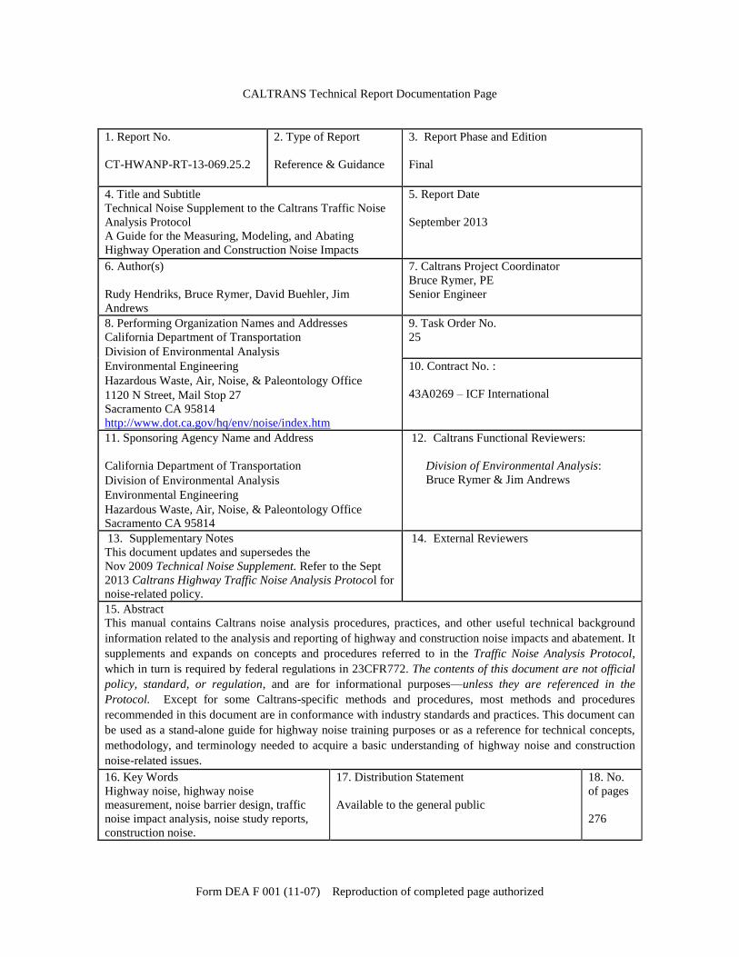
CALTRANS Technical Report Documentation Page
1. Report No.
CT-HWANP-RT-13-069.25.2
2. Type of Report
Reference & Guidance
3. Report Phase and Edition
Final
4. Title and Subtitle
Technical Noise Supplement to the Caltrans Traffic Noise
Analysis Protocol
A Guide for the Measuring, Modeling, and Abating
Highway Operation and Construction Noise Impacts
5. Report Date
September 2013
6. Author(s)
Rudy Hendriks, Bruce Rymer, David Buehler, Jim
Andrews
7. Caltrans Project Coordinator
Bruce Rymer, PE
Senior Engineer
8. Performing Organization Names and Addresses
California Department of Transportation
Division of Environmental Analysis
Environmental Engineering
Hazardous Waste, Air, Noise, & Paleontology Office
1120 N Street, Mail Stop 27
Sacramento CA 95814
http://www.dot.ca.gov/hq/env/noise/index.htm
9. Task Order No.
25
10. Contract No. :
43A0269 – ICF International
11. Sponsoring Agency Name and Address
California Department of Transportation
Division of Environmental Analysis
Environmental Engineering
Hazardous Waste, Air, Noise, & Paleontology Office
Sacramento CA 95814
12. Caltrans Functional Reviewers:
Division of Environmental Analysis:
Bruce Rymer & Jim Andrews
13. Supplementary Notes
This document updates and supersedes the
Nov 2009 Technical Noise Supplement. Refer to the Sept
2013 Caltrans Highway Traffic Noise Analysis Protocol for
noise-related policy.
14. External Reviewers
15. Abstract
This manual contains Caltrans noise analysis procedures, practices, and other useful technical background
information related to the analysis and reporting of highway and construction noise impacts and abatement. It
supplements and expands on concepts and procedures referred to in the Traffic Noise Analysis Protocol,
which in turn is required by federal regulations in 23CFR772. The contents of this document are not official
policy, standard, or regulation, and are for informational purposes—unless they are referenced in the
Protocol. Except for some Caltrans-specific methods and procedures, most methods and procedures
recommended in this document are in conformance with industry standards and practices. This document can
be used as a stand-alone guide for highway noise training purposes or as a reference for technical concepts,
methodology, and terminology needed to acquire a basic understanding of highway noise and construction
noise-related issues.
16. Key Words
Highway noise, highway noise
measurement, noise barrier design, traffic
noise impact analysis, noise study reports,
construction noise.
17. Distribution Statement
Available to the general public
18. No.
of pages
276

This page intentionally left blank
Technical Noise Supplement to the Caltrans Traffic Noise Analysis Protocol
A Guide for Measuring, Modeling, and Abating Highway
Operation and Construction Noise Impacts
California Department of Transportation
Division of Environmental Analysis
Environmental Engineering
Hazardous Waste, Air, Noise, Paleontology Office
1120 N Street, Room 4301 MS27
Sacramento, CA 95814
Contact: Bruce Rymer
916/653-6073
September 2013
© 2013 California Department of Transportation

California Department of Transportation. 2013. Technical Noise Supplement to
the Caltrans Traffic Noise Analysis Protocol. September. Sacramento, CA.

Technical Noise Supplement Page i September 2013
Contents
Page Tables .................................................................................................... vi Figures .................................................................................................. viii Acronyms and Abbreviations .................................................................. xii Acknowledgements ............................................................................... xiv
Section 1 Introduction and Overview .................................................................1-1 1.1 Introduction ................................................................................1-1 1.2 Overview ....................................................................................1-2
Section 2 Basics of Highway Noise ....................................................................2-1 2.1 Physics of Sound .......................................................................2-1
2.1.1 Sound, Noise, and Acoustics ...............................................2-1 2.1.2 Speed of Sound ...................................................................2-2 2.1.3 Sound Characteristics ..........................................................2-3
2.1.3.1 Frequency, Wavelength, and Hertz...........................2-3 2.1.3.2 Sound Pressure Levels and Decibels .......................2-7 2.1.3.3 Root Mean Square and Relative Energy ...................2-8 2.1.3.4 Relationship between Sound Pressure
Level, Relative Energy, Relative Pressure, and Pressure ............................................2-9
2.1.3.5 Adding, Subtracting, and Averaging Sound Pressure Levels........................................... 2-11
2.1.3.6 A-Weighting and Noise Levels ................................ 2-18 2.1.3.7 Octave and One-Third-Octave Bands
and Frequency Spectra .......................................... 2-21 2.1.3.8 White and Pink Noise ............................................. 2-27
2.1.4 Sound Propagation ............................................................ 2-27 2.1.4.1 Geometric Spreading from Point and
Line Sources .......................................................... 2-27 2.1.4.2 Ground Absorption ................................................. 2-30 2.1.4.3 Atmospheric Effects and Refraction ........................ 2-31 2.1.4.4 Shielding by Natural and Manmade
Features, Noise Barriers, Diffraction, and Reflection ........................................................ 2-35
2.2 Effects of Noise and Noise Descriptors .................................... 2-43 2.2.1 Human Reaction to Sound ................................................. 2-43
2.2.1.1 Human Response to Changes in Noise Levels ..................................................................... 2-44
2.2.2 Describing Noise ................................................................ 2-46
Page ii September 2013
Technical Noise Supplement
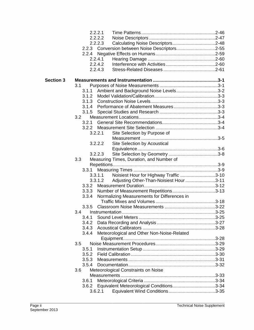
2.2.2.1 Time Patterns ......................................................... 2-46 2.2.2.2 Noise Descriptors ................................................... 2-47 2.2.2.3 Calculating Noise Descriptors ................................. 2-48
2.2.3 Conversion between Noise Descriptors .............................. 2-55 2.2.4 Negative Effects on Humans .............................................. 2-59
2.2.4.1 Hearing Damage .................................................... 2-60 2.2.4.2 Interference with Activities ...................................... 2-60 2.2.4.3 Stress-Related Diseases ........................................ 2-61
Section 3 Measurements and Instrumentation ..................................................3-1 3.1 Purposes of Noise Measurements .............................................3-1
3.1.1 Ambient and Background Noise Levels ................................3-2 3.1.2 Model Validation/Calibration .................................................3-3 3.1.3 Construction Noise Levels ....................................................3-3 3.1.4 Performance of Abatement Measures ..................................3-3 3.1.5 Special Studies and Research .............................................3-3
3.2 Measurement Locations .............................................................3-4 3.2.1 General Site Recommendations...........................................3-4 3.2.2 Measurement Site Selection ................................................3-4
3.2.2.1 Site Selection by Purpose of Measurement ...........................................................3-5
3.2.2.2 Site Selection by Acoustical Equivalence ..............................................................3-6
3.2.2.3 Site Selection by Geometry ......................................3-8 3.3 Measuring Times, Duration, and Number of
Repetitions .................................................................................3-9 3.3.1 Measuring Times .................................................................3-9
3.3.1.1 Noisiest Hour for Highway Traffic ........................... 3-10 3.3.1.2 Adjusting Other-Than-Noisiest Hour ....................... 3-11
3.3.2 Measurement Duration ....................................................... 3-12 3.3.3 Number of Measurement Repetitions ................................. 3-13 3.3.4 Normalizing Measurements for Differences in
Traffic Mixes and Volumes .............................................. 3-18 3.3.5 Classroom Noise Measurements ....................................... 3-22
3.4 Instrumentation ........................................................................ 3-25 3.4.1 Sound Level Meters ........................................................... 3-25 3.4.2 Data Recording and Analysis ............................................. 3-27 3.4.3 Acoustical Calibrators ........................................................ 3-28 3.4.4 Meteorological and Other Non-Noise-Related
Equipment ....................................................................... 3-28 3.5 Noise Measurement Procedures .............................................. 3-29
3.5.1 Instrumentation Setup ........................................................ 3-29 3.5.2 Field Calibration ................................................................. 3-30 3.5.3 Measurements ................................................................... 3-31 3.5.4 Documentation ................................................................... 3-32
3.6 Meteorological Constraints on Noise Measurements ......................................................................... 3-33
3.6.1 Meteorological Criteria ....................................................... 3-34 3.6.2 Equivalent Meteorological Conditions................................. 3-34
3.6.2.1 Equivalent Wind Conditions .................................... 3-35
Technical Noise Supplement Page iii September 2013
3.6.2.2 Equivalent Temperature and Cloud Cover ...................................................................... 3-36
3.6.2.3 Equivalent Humidity ................................................ 3-36 3.7 Quality Assurance .................................................................... 3-36
Section 4 Detailed Analysis for Traffic Noise Impacts ......................................4-1 4.1 Gathering Information ................................................................4-1 4.2 Identifying Existing and Future Land Use and
Applicable Noise Abatement Criteria ..........................................4-1 4.3 Determining Existing Noise Levels .............................................4-3
4.3.1 Selecting Noise Receivers and Noise Measurement Sites ...........................................................4-3
4.3.1.1 Receptors and Receivers .........................................4-3 4.3.1.2 Noise Measurement Sites .........................................4-6
4.3.2 Measuring Existing Noise Levels ..........................................4-6 4.3.3 Modeling Existing Noise Levels ............................................4-7
4.4 Validating/Calibrating the Prediction Model ................................4-7 4.4.1 Routine Model Calibration ....................................................4-8
4.4.1.1 Introduction ...............................................................4-8 4.4.1.2 Limitations ................................................................4-8 4.4.1.3 Pertinent Site Conditions ..........................................4-9 4.4.1.4 Procedures ............................................................. 4-10 4.4.1.5 Cautions and Challenges ........................................ 4-11 4.4.1.6 Tolerances .............................................................. 4-13 4.4.1.7 Common Dilemmas ................................................ 4-13
4.5 Predicting Future Noise Levels ................................................ 4-14 4.5.1 FHWA TNM Overview ........................................................ 4-15
4.5.1.1 TNM Reference Energy Mean Emission Levels ..................................................................... 4-15
4.5.1.2 Noise Level Computations ...................................... 4-18 4.5.1.3 Propagation, Shielding, and Ground
Effects .................................................................... 4-19 4.5.1.4 Parallel Barrier Analysis .......................................... 4-19
4.6 Comparing Results with Appropriate Criteria ........................... 4-20 4.7 Evaluating Noise Abatement Options ....................................... 4-20
Section 5 Noise Barrier Design Considerations ................................................5-1 5.1 Acoustical Design Considerations ..............................................5-1
5.1.1 Barrier Material and Transmission Loss ...............................5-3 5.1.2 Barrier Location ....................................................................5-6 5.1.3 Barrier Dimensions ............................................................. 5-13
5.1.3.1 Height ..................................................................... 5-15 5.1.3.2 Length .................................................................... 5-21
5.1.4 Barrier Shape ..................................................................... 5-23 5.1.5 Barrier Insertion Loss vs. Attenuation ................................. 5-25 5.1.6 Background Noise Levels................................................... 5-26 5.1.7 Reflected Noise and Noise Barriers ................................... 5-27
5.1.7.1 Noise Reflection ..................................................... 5-27 5.1.7.2 Single Barriers ........................................................ 5-29 5.1.7.3 Modeling Single Barrier Reflections ........................ 5-35 5.1.7.4 Parallel Barriers ...................................................... 5-37
Page iv September 2013
Technical Noise Supplement
5.1.7.5 Reflections off Structures and Canyon Effects .................................................................... 5-41
5.1.7.6 Double-Deck Bridge Reflections ............................. 5-43 5.1.7.7 Minimizing Reflections ............................................ 5-51
5.1.8 Miscellaneous Acoustical Design Considerations ................................................................ 5-52
5.1.8.1 Maintenance Access behind Noise Barriers ................................................................... 5-52
5.1.8.2 Emergency Access Gates in Noise Barriers ................................................................... 5-54
5.1.8.3 Drainage Openings in Noise Barriers ...................... 5-54 5.1.8.4 Vegetation as Noise Barriers .................................. 5-55
5.2 Non-Acoustical Considerations ................................................ 5-55 5.2.1 Safety................................................................................. 5-55 5.2.2 Aesthetics .......................................................................... 5-56
Section 6 Noise Study Reports ...........................................................................6-1 6.1 Outline .......................................................................................6-2 6.2 Summary ...................................................................................6-4 6.3 Noise Impact Technical Study ....................................................6-4
6.3.1 Introduction ..........................................................................6-4 6.3.2 Project Description ...............................................................6-4 6.3.3 Fundamentals of Traffic Noise..............................................6-5 6.3.4 Federal and State Standards and Policies ...........................6-6 6.3.5 Study Methods and Procedures ...........................................6-6 6.3.6 Existing Noise Environment .................................................6-7 6.3.7 Future Noise Environment, Impacts, and
Considered Abatement ......................................................6-8 6.3.8 Construction Noise ............................................................. 6-10 6.3.9 References ........................................................................ 6-10
6.4 Appendices .............................................................................. 6-16
Section 7 Non-Routine Considerations and Issues ...........................................7-1 7.1 Noise Barrier Issues ...................................................................7-1
7.1.1 Effects of Noise Barriers on Distant Receivers .....................7-2 7.1.1.1 Background ..............................................................7-2 7.1.1.2 Results of Completed Studies ...................................7-3 7.1.1.3 Studying the Effects of Noise Barriers
on Distant Receivers ................................................7-7 7.1.2 Shielding Provided by Vegetation .........................................7-7
7.2 Sound Intensity and Power ........................................................7-8 7.2.1 Sound Power .......................................................................7-9 7.2.2 Sound Intensity .................................................................. 7-10
7.3 Tire/Pavement Noise ............................................................... 7-13 7.4 Insulating Facilities from Highway Noise .................................. 7-16 7.5 Construction Noise Analysis, Monitoring, and
Abatement ............................................................................... 7-17 7.5.1 Consideration of Construction Noise during
Project Development Phase ............................................ 7-20 7.5.2 Noise Monitoring during Construction ................................ 7-23 7.5.3 Construction Noise Abatement ........................................... 7-26
Technical Noise Supplement Page v September 2013
7.5.3.1 Abatement at Source .............................................. 7-26 7.5.3.2 Abatement in Path .................................................. 7-26 7.5.3.3 Abatement at Receiver ........................................... 7-27 7.5.3.4 Community Awareness ........................................... 7-27
7.6 Earthborne Vibration ................................................................ 7-27 7.7 Occupational Hearing Loss and OSHA Noise
Standards ................................................................................ 7-28 7.7.1 Noise-Induced Hearing Loss .............................................. 7-29 7.7.2 OSHA Noise Standards ..................................................... 7-29
7.8 Effects of Transportation and Construction Noise on Marine Life and Wildlife (Bioacoustics) ................................ 7-31
Section 8 Glossary ...............................................................................................8-1
Appendix A References Cited
Page vi September 2013
Technical Noise Supplement
Tables
Page
2-1 Wavelength of Various Frequencies ......................................................2-6
2-2 Relationship between Sound Pressure Level, Relative Energy, Relative Pressure, and Sound Pressure ................................. 2-10
2-3 Decibel Addition .................................................................................. 2-14
2-4 A-Weighting Adjustments for One-Third-Octave Center Frequencies ........................................................................................ 2-19
2-5 Typical Noise Levels ........................................................................... 2-20
2-6 Standardized Band Numbers, Center Frequencies, One-Third-Octave and Octave Bands, and Octave Band Ranges ................................................................................................ 2-22
2-7 Tabular Form of Octave Band Spectrum ............................................. 2-24
2-8 Tabular Form of One-Third Octave Band Spectrum ............................ 2-25
2-9 Adjusting Linear Octave Band Spectrum to A-Weighted Spectrum ............................................................................................. 2-26
2-10 Relationship between Noise Level Change, Factor Change in Relative Energy, and Perceived Change ......................................... 2-45
2-11 Common Noise Descriptors ................................................................. 2-48
2-12 Noise Samples for L10 Calculation ...................................................... 2-49
2-13 Noise Samples for Leq Calculation ...................................................... 2-51
2-14 Noise Samples for Ldn Calculations .................................................... 2-52
2-15 Leq/Ldn Conversion Factors................................................................ 2-58
2-16 Ldn/CNEL Corrections () (Must Be Added to Ldn to Obtain CNEL) ...................................................................................... 2-59
Technical Noise Supplement Page vii September 2013
3-1 Suggested Measurement Durations .................................................... 3-12
3-2 Maximum Allowable Standard Deviations for a 95% Confidence Interval for Mean Measurement of about 1 dBA ................ 3-17
3-3 Equivalent Vehicles Based on Federal Highway Administration Traffic Noise Model Reference Energy Mean Emission Levels ......................................................................... 3-19
3-4 Classes of Wind Conditions ................................................................. 3-35
3-5 Cloud Cover Classes ........................................................................... 3-36
4-1 Activity Categories and Noise Abatement Criteria (23 CFR 772) .......................................................................................................4-2
4-2 TNM Constants for Vehicle Types ....................................................... 4-17
5-1 Approximate Transmission Loss Values for Common Materials................................................................................................5-4
5-2 Contribution of Reflections for Special Case Where W = 2S, D = W, and NRC = 0.05 ................................................................ 5-40
5-3 Summary of Reflective Noise Contributions and Cumulative Noise Levels ..................................................................... 5-51
6-1 Noise Study Report Outline ...................................................................6-2
6-2 Existing Noise Levels (Example) ......................................................... 6-11
6-3 Predicted Traffic Noise Impacts (Example) .......................................... 6-12
6-4 Noise Abatement Predicted Noise Levels and Insertion Loss (dBA) for Soundwall 1 at Right-of-Way (Example) ....................... 6-13
6-5 Data for Reasonableness Determination (Example) ............................ 6-14
6-6 Roadway and Barrier Geometries (Example) ...................................... 6-15
6-7 Model Calibration (Example) ............................................................... 6-16
7-1 FHWA Building Noise Reduction Factors ............................................ 7-17
7-2 Typical Construction Equipment Noise ................................................ 7-21
7-3 Table G-16 Permissible Noise Exposure ............................................. 7-30
Page viii September 2013
Technical Noise Supplement
Figures
Page
2-1 Sound Pressure vs. Particle Velocity .....................................................2-4
2-2 Frequency and Wavelength ...................................................................2-5
2-3 Peak and Root Mean Square Sound Pressure ......................................2-9
2-4 A-Weighting Network ........................................................................... 2-19
2-5 Typical Octave Band Frequency Spectrum .......................................... 2-23
2-6 Typical One-Third-Octave Band Frequency Spectrum ......................... 2-25
2-7 Point Source Propagation (Spherical Spreading) ................................. 2-28
2-8 Change in Noise Level with Distance from Spherical Spreading .......... 2-29
2-9 Line Source Propagation (Cylindrical Spreading) ................................ 2-30
2-10 Wind Effects on Noise Levels .............................................................. 2-32
2-11 Effects of Temperature Gradients on Noise ......................................... 2-34
2-12 Alteration of Sound Paths after Inserting a Noise Barrier between Source and Receiver ............................................................. 2-37
2-13 Diffraction of Sound Waves ................................................................. 2-39
2-14 Path Length Difference between Direct and Diffracted Noise Paths .... 2-40
2-15 Barrier Attenuation (∆B) vs. Fresnel Number (N0) for Infinitely Long Barriers ......................................................................... 2-41
2-16 Direct Noise Path Grazing Top of Barrier, Resulting in 5 dBA of Attenuation ...................................................................................... 2-42
2-17 Negative Diffraction, Which Provides Some Noise Attenuation ............ 2-43
2-18 Different Noise Level vs. Time Patterns ............................................... 2-46
Technical Noise Supplement Page ix September 2013
2-19 Relationship between Ldn and Leq(h)pk .................................................. 2-58
2-20 Interference of Conversation from Background Noise.......................... 2-61
3-1 Typical Measurement Site Locations .....................................................3-7
3-2 Typical Noise Measurement Site Locations ...........................................3-8
3-3 Receiver Partially Shielded by Top of Cut vs. Unshielded Receiver.......3-9
3-4 Classroom Noise Measurements (Reconstruction of Existing Freeway) ............................................................................................. 3-23
3-5 Classroom Noise Measurements (Project on New Alignment with Artificial Sound Source) ................................................................ 3-24
4-1 A-Weighted Baseline FHWA TNM REMEL Curves .............................. 4-18
5-1 Alteration of Noise Paths by a Noise Barrier ..........................................5-3
5-2 Barrier Diffraction ..................................................................................5-3
5-3 Path Length Difference ..........................................................................5-7
5-4 Barrier Attenuation as a Function of Location (At-Grade Highway)—Barrier Attenuation Is Least When Barrier Is Located Halfway Between the Source and Receiver b; the Best Locations Are Near the Source a or Receiver c .............................5-8
5-5 Typical Barrier Location for Depressed Highways .................................5-9
5-6 Typical Barrier Location for Elevated Highways ................................... 5-10
5-7 Barriers for Cut and Fill Transitions ..................................................... 5-11
5-8 Barriers for Highway on Fill with Off-Ramp .......................................... 5-12
5-9 Barriers for Highway in Cut with Off-Ramp .......................................... 5-13
5-10 Actual Noise Barrier Height Depends on Site Geometry and Terrain Topography (Same Barrier Attenuation for a, b, c, and d) ......................................................................................................... 5-14
5-11 Noise Barrier Length Depends on Size of the Area to Be Shielded and Site Geometry and Topography ..................................... 5-14
5-12 Soundwall Attenuation vs. Height for At-Grade Freeway ..................... 5-15
5-13 Soundwall Attenuation vs. Height for 25-Foot Depressed Freeway .............................................................................................. 5-17
Page x September 2013
Technical Noise Supplement
5-14 Loss of Soft-Site Characteristics from Constructing a Noise Barrier ................................................................................................. 5-18
5-15 Determination of Critical Lane for Line-of-Sight Height ........................ 5-20
5-16 Recommended Line-of-Sight Break Limits ........................................... 5-20
5-17 Barrier Extended Far Enough to Protect End Receivers ...................... 5-21
5-18 4D Rule ............................................................................................... 5-22
5-19 Barrier Wrapped around End Receivers, an Effective Alternative ........ 5-23
5-20 Thin Screen vs. Berm (Berm Gives More Barrier Attenuation) ............. 5-24
5-21 Various Wall Shapes (Minimal Benefit for Extra Cost) ......................... 5-24
5-22 Barrier Insertion Loss vs. Attenuation .................................................. 5-25
5-23 Single-Barrier Reflection (Simplest Representation) ............................ 5-29
5-24 Single-Barrier Reflections (Infinite Line Source and Noise Barrier) ...... 5-30
5-25 Single-Barrier Reflection (More Accurate Representation) .................. 5-31
5-26 Noise Increases from Single-Barrier Reflections .................................. 5-32
5-27 Single-Barrier Reflection (Direct Noise Shielded, Reflected Noise Not Shielded) ............................................................................ 5-33
5-28 Single-Barrier Reflection (Noise Barrier on Top of Opposite Cut) ........ 5-34
5-29 Highway and Noise Barrier on Fill ....................................................... 5-34
5-30 Placement of Image Sources (Cross Sectional View) .......................... 5-35
5-31 Placement of Image Sources (Plan View) ............................................ 5-36
5-32 Various Reflective Noise Paths for Parallel Noise Barriers .................. 5-39
5-33 W/HAVG Ratio Should be 10:1 or Greater ............................................. 5-41
5-34 Noise Reflection off Structure .............................................................. 5-42
5-35 Double-Deck Structure Reflections, First Reflective Path .................... 5-44
5-36 Multiple Reflective Paths ..................................................................... 5-49
5-37 Barrier Offset with Solid Gate .............................................................. 5-53
Technical Noise Supplement Page xi September 2013
5-38 Barrier Overlap Offset 2.5 to 3 Times the Width of the Access Opening .................................................................................. 5-53
5-39 Spatial Relationship of Barrier to Adjoining Land Use .......................... 5-57
7-1 Schematic of a Sound Intensity Probe ................................................. 7-12
7-2 Side-by-Side Microphone Probe .......................................................... 7-12
7-3 Sound Power Measurement Area ........................................................ 7-13
7-4 Measuring One Piece of Equipment .................................................... 7-24
7-5 Measuring Multiple Pieces of Equipment Operating in Same Area ...... 7-25
Page xii September 2013
Technical Noise Supplement
Acronyms and Abbreviations
change
°F degrees Farenheit AASHTO
American Association of State Highway and Transportation Officials
AC asphalt concrete ADT average daily traffic ANSI American National Institute of Standards B
bels
Caltrans
California Department of Transportation
CFR Code of Federal Regulations CNEL community noise equivalent level cps cycles per second dB
decibels
dB/s decibels per second dBA DGAC
A-weighted decibels dense-graded asphalt concrete
EWNR
Exterior Wall Noise Rating
FHWA Federal Highway Administration ft/s feet per second GPS
global positioning system
Guidance Manual Technical Guidance Manual on the Effects on the Assessment and Mitigation of Hydroacoustic Effects of Pile Driving Sound on Fish
Hz hertz I- Interstate kHz kilohertz km/hr kilometers per hour kVA kilovolt-amperes Ldn
day-night noise level
Leq equivalent noise level Lmax maximum noise level
Technical Noise Supplement Page xiii September 2013
m/s meters per second mph miles per hour N
Newton
N/m2 Newton per square meter NAC noise abatement criteria NADR Noise Abatement Decision Report NIST National Institute of Standards and Technology Nm Newton meter NRC noise reduction coefficient OBSI
on-board sound intensity
OGAC OSHA
open-graded aspalt concrete Occupational Safety and Health Administration
PCC Portland concrete cement PLD path length difference Protocol Traffic Noise Analysis Protocol psi pounds per square inch pW picowatt REMEL
Reference Energy Mean Emission Level
rms root mean square SPL sound pressure level SR State Route STC Sound Transmission Class TeNS
Technical Noise Supplement
TL transmission loss TNM Traffic Noise Model VNTSC Volpe National Transportation Systems Center vph vehicles per hour W
watts
W/m2 watts per square meter µN/m2
microNewtons per square meter
µPa micro Pascals
Page xiv September 2013
Technical Noise Supplement
Acknowledgements
Rudy Hendriks (ICF Jones & Stokes; California Department of
Transportation [retired])—principal author
Bruce Rymer (California Department of Transportation)—technical reviewer
Jim Andrews (California Department of Transportation)—technical reviewer
Dave Buehler (ICF International)—technical editor
Technical Noise Supplement Page xv September 2013
Dedication:
This edition of the Technical Noise Supplement is dedicated to Rudy Hendriks whose early work
substantially contributed to the science of highway acoustics.

Page xvi September 2013
Technical Noise Supplement
This page intentionally left blank
Technical Noise Supplement Page 1-1
September 2013
Section 1 Introduction and Overview
1.1 Introduction This 2013 Technical Noise Supplement (TeNS) to the California Department of Transportation (Caltrans) Traffic Noise Analysis Protocol for New Highway Construction, Reconstruction, and Retrofit Barrier Projects (Protocol) (California Department of Transportation 2011) is an updated version of the 2009 TeNS. This version of the TeNS is compatible with applicable sections of the 2011 Protocol that were prepared in response to changes to Title 23 Part 772 of the Code of Federal Regulations (CFR) which were published in July 2010. The current Protocol was approved by the Federal Highway Administration (FHWA) and became effective on July 13, 2011. Be sure to check for updates to the Protocol.
The purpose of this document is to provide technical background information on transportation-related noise in general and highway traffic noise in particular. It is designed to elaborate on technical concepts and procedures referred to in the Protocol. The contents of the TeNS are for informational purposes; unless they are referenced in the Protocol, the contents of this document are not official policy, standard, or regulation. Except for some Caltrans-specific methods and procedures, most methods and procedures recommended in TeNS are in conformance with industry standards and practices.
This document can be used as a stand-alone document for training purposes or as a reference for technical concepts, methodology, and terminology needed to acquire a basic understanding of transportation noise with emphasis on highway traffic noise.
Revisions to this document are listed below.
Removal of references and discussion relating to traffic noise models that preceded the current FHWA Traffic Noise Model (TNM).
California Department of Transportation Introduction and Overview
Page 1-2 September 2013
Technical Noise Supplement
Abbreviated discussions of several topics such as bioacoustics and
quieter pavement that are now covered in more detail in newer
technical references.
Elimination of metric units in accordance with Caltrans current
standards. The exception to this is units of pressure that are
traditionally expressed in metric units such as micro-pascals.
Removal of the traffic noise analysis screening procedure which was
removed from the Protocol.
Removal of obsolete information.
The 2009 version of TeNS will remain available on the Caltrans website
as a reference for information that has been removed from this edition.
The 2009 version of TeNS contains a number of measurement procedures
for non-routine noise studies.
1.2 Overview
The TeNS consists of eight sections. Except for Section 1, each covers a
specific subject of highway noise. A brief description of the subjects
follows.
Section 1, Introduction and Overview, summarizes the subjects
covered in the TeNS.
Section 2, Basics of Highway Noise, covers the physics of sound as it
pertains to characteristics and propagation of highway noise, effects of
noise on humans, and ways of describing noise.
Section 3, Measurements and Instrumentation, provides background
information on noise measurements, and discusses various noise-
measuring instruments and operating procedures.
Section 4, Detailed Analysis for Traffic Noise Impacts, provides
guidance for conducting detailed traffic noise impact analysis studies.
This section includes identifying land use, selecting receptors,
determining existing noise levels, predicting future noise levels, and
determining impacts.
Section 5, Detailed Analysis for Noise Barrier Design Considerations,
outlines the major aspects that affect the acoustical design of noise
barriers, including the dimensions, location, and material; optimization
of noise barriers; possible noise reflections; acoustical design of
overlapping noise barriers (to provide maintenance access to areas
California Department of Transportation Introduction and Overview
Technical Noise Supplement Page 1-3 September 2013
behind barriers); and drainage openings in noise barriers. Challenges
and cautions associated with noise barrier design are also discussed.
Section 6, Noise Study Reports, discusses the contents of noise study
reports.
Section 7, Non-Routine Considerations and Issues, covers non-routine
situations involving the effects of noise on distant receptors, use of
sound intensity and sound power as tools in characterizing sound
sources, pavement noise, noise monitoring for insulating facilities,
construction noise, earthborne vibrations, California Occupational
Safety and Health Administration (OSHA) noise standards, and effects
and abatement of transportation-related noise on marine and wildlife.
Section 8, Glossary, provides terminology and definitions common in
transportation noise.
Appendix A, References Cited, provides a listing of literature directly
cited or used for reference in the TeNS.

California Department of Transportation Introduction and Overview
Page 1-4 September 2013
Technical Noise Supplement
This page intentionally left blank
Technical Noise Supplement Page 2-1 September 2013
Section 2
Basics of Highway Noise
The following sections introduce the fundamentals of sound and provide
sufficient detail to understand the terminology and basic factors involved
in highway traffic noise prediction and analysis. Those who are actively
involved in noise analysis are encouraged to seek out more detailed
textbooks and reference books to acquire a deeper understanding of the
subject.
2.1 Physics of Sound
2.1.1 Sound, Noise, and Acoustics
Sound is a vibratory disturbance created by a moving or vibrating source
in the pressure and density of a gaseous or liquid medium or in the elastic
strain of a solid that is capable of being detected by the hearing organs.
Sound may be thought of as the mechanical energy of a vibrating object
transmitted by pressure waves through a medium to human (or animal)
ears. The medium of primary concern is air. In absence of any other
qualifying statements, sound is considered airborne sound, as opposed to
structure- or earthborne sound, for example.
Noise is defined as sound that is loud, unpleasant, unexpected, or
undesired. It therefore may be classified as a more specific group of
sounds. Although the terms sound and noise are often used synonymously,
perceptions of sound and noise are highly subjective.
Sound is actually a process that consists of three components: source,
path, and receiver. All three components must be present for sound to
exist. Without a source, no sound pressure waves would be produced.
Similarly, without a medium, sound pressure waves would not be
transmitted. Finally, sound must be received—a hearing organ, sensor, or
other object must be present to perceive, register, or be affected by sound.
In most situations, there are many different sound sources, paths, and
receivers.
California Department of Transportation Basics of Highway Noise
Page 2-2 September 2013
Technical Noise Supplement
In the context of an analysis pursuant to 23 CFR 772 the term receptor
means a single dwelling unit or the equivalent of a single dwelling unit. A
receiver is a single point that can represent one receptor or multiple
receptors. As an example it is common when modeling traffic noise to use
a single receiver in the model to represent multiple receptors. Acoustics is
the field of science that deals with the production, propagation, reception,
effects, and control of sound. The field is very broad, and transportation-
related noise and abatement addresses only a small, specialized part of
acoustics.
2.1.2 Speed of Sound
When the surface of an object vibrates in air, it compresses a layer of air
as the surface moves outward and produces a rarefied zone as the surface
moves inward. This results in a series of high and low air pressure waves
(relative to the steady ambient atmospheric pressure) alternating in
sympathy with the vibrations. These pressure waves, not the air itself,
move away from the source at the speed of sound, approximately 1,126
feet per second (ft/s) in air with a temperature of 68 degrees Fahrenheit
(°F). The speed of sound can be calculated from the following formula:
c = 1 401.P
(2-1)
Where:
c = speed of sound at a given temperature, in ft/s
P = air pressure in pounds per square foot (pounds/ft2)
= air density in slugs per cubic foot (slugs/ft3)
1.401 = ratio of the specific heat of air under constant pressure to that of air in a
constant volume
For a given air temperature and relative humidity, the ratio P/ tends to
remain constant in the atmosphere because the density of air will reduce or
increase proportionally with changes in pressure. Therefore, the speed of
sound in the atmosphere is independent of air pressure. When air
temperature changes, changes, but P does not. Therefore, the speed of
sound is temperature-dependent, as well as somewhat humidity-dependent
because humidity affects the density of air. The effects of the latter with
regard to the speed of sound, however, can be ignored for the purposes of
the TeNS. The fact that the speed of sound changes with altitude has
nothing to do with the change in air pressure and is only caused by the
change in temperature.
California Department of Transportation Basics of Highway Noise
Technical Noise Supplement Page 2-3 September 2013
For dry air of 32ºF, is 0.002509 slugs/ft3. At a standard air pressure of
29.92 inches Hg, pressure is 14.7 pounds per square inch (psi) or 2,118
pounds/ft2. Using Equation 2-1, the speed of sound for standard pressure
and temperature can be calculated as follows:
c = )002509.0
118,2)(401.1( = 1,087 ft/s.
From this base value, the variation with temperature is described by the
following equation:
459.7
T+11051.3=c
f
ft/s (2-2)
Where:
c = speed of sound
Tf = temperature in degrees Fahrenheit (include minus sign for less than 0ºF)
The above equations show that the speed of sound increases or decreases
as the air temperature increases or decreases, respectively. This
phenomenon plays an important role in the atmospheric effects on noise
propagation, specifically through the process of refraction, which is
discussed in Section 2.1.4.3.
2.1.3 Sound Characteristics
In its most basic form, a continuous sound can be described by its
frequency or wavelength (pitch) and amplitude (loudness).
2.1.3.1 Frequency, Wavelength, and Hertz
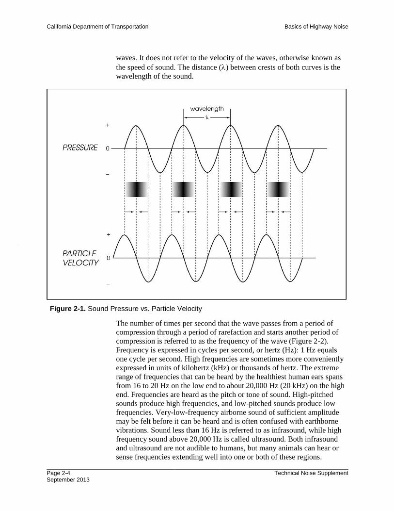
For a given single pitch, the sound pressure waves are characterized by a
sinusoidal periodic (i.e., recurring with regular intervals) wave, as shown
in Figure 2-1. The upper curve shows how sound pressure varies above
and below the ambient atmospheric pressure with distance at a given time.
The lower curve shows how particle velocity varies above 0 (molecules
moving right) and below 0 (molecules moving left). Please note that when
the pressure fluctuation is at 0, the particle velocity is at its maximum,
either in the positive or negative direction; when the pressure is at its
positive or negative peak, the particle velocity is at 0. Particle velocity
describes the motion of the air molecules in response to the pressure
California Department of Transportation Basics of Highway Noise
Page 2-4 September 2013
Technical Noise Supplement
waves. It does not refer to the velocity of the waves, otherwise known as
the speed of sound. The distance () between crests of both curves is the
wavelength of the sound.
The number of times per second that the wave passes from a period of
compression through a period of rarefaction and starts another period of
compression is referred to as the frequency of the wave (Figure 2-2).
Frequency is expressed in cycles per second, or hertz (Hz): 1 Hz equals
one cycle per second. High frequencies are sometimes more conveniently
expressed in units of kilohertz (kHz) or thousands of hertz. The extreme
range of frequencies that can be heard by the healthiest human ears spans
from 16 to 20 Hz on the low end to about 20,000 Hz (20 kHz) on the high
end. Frequencies are heard as the pitch or tone of sound. High-pitched
sounds produce high frequencies, and low-pitched sounds produce low
frequencies. Very-low-frequency airborne sound of sufficient amplitude
may be felt before it can be heard and is often confused with earthborne
vibrations. Sound less than 16 Hz is referred to as infrasound, while high
frequency sound above 20,000 Hz is called ultrasound. Both infrasound
and ultrasound are not audible to humans, but many animals can hear or
sense frequencies extending well into one or both of these regions.
Figure 2-1. Sound Pressure vs. Particle Velocity
California Department of Transportation Basics of Highway Noise
Technical Noise Supplement Page 2-5 September 2013
Ultrasound also has various applications in industrial and medical
processes, specifically cleaning, imaging, and drilling.
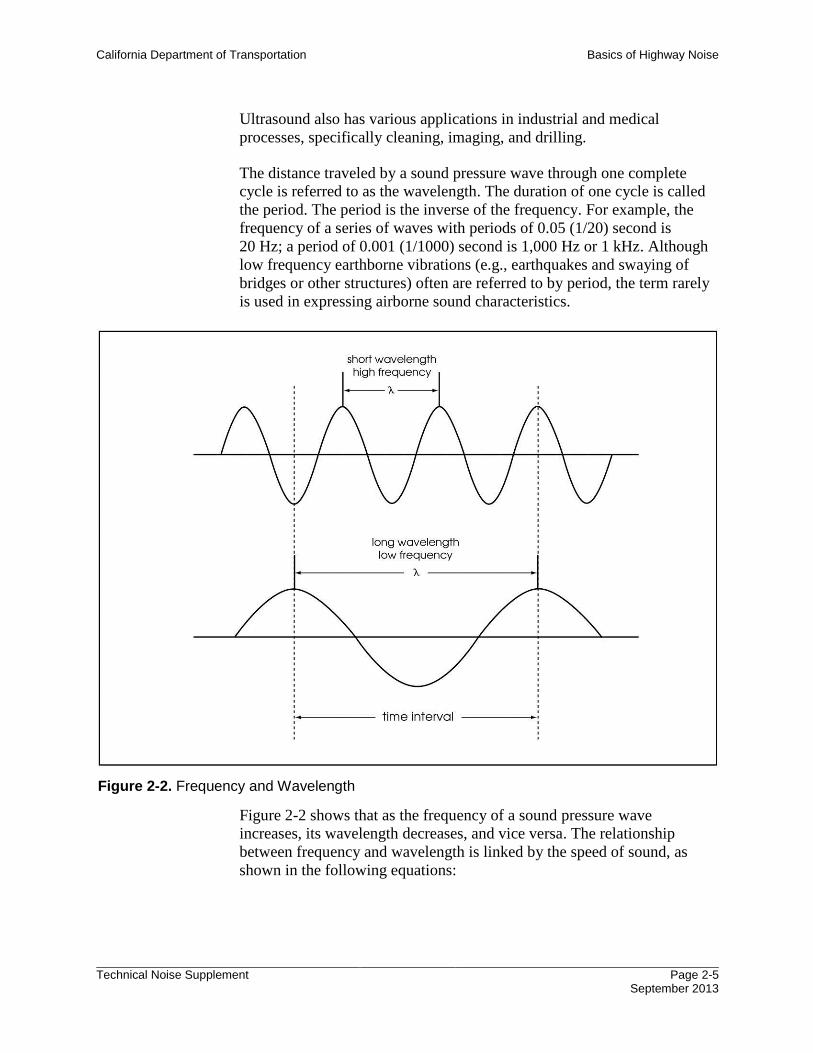
The distance traveled by a sound pressure wave through one complete
cycle is referred to as the wavelength. The duration of one cycle is called
the period. The period is the inverse of the frequency. For example, the
frequency of a series of waves with periods of 0.05 (1/20) second is
20 Hz; a period of 0.001 (1/1000) second is 1,000 Hz or 1 kHz. Although
low frequency earthborne vibrations (e.g., earthquakes and swaying of
bridges or other structures) often are referred to by period, the term rarely
is used in expressing airborne sound characteristics.
Figure 2-2 shows that as the frequency of a sound pressure wave
increases, its wavelength decreases, and vice versa. The relationship
between frequency and wavelength is linked by the speed of sound, as
shown in the following equations:
Figure 2-2. Frequency and Wavelength
California Department of Transportation Basics of Highway Noise
Page 2-6 September 2013
Technical Noise Supplement
= cf (2-3)
f = c
(2-4)
c = f (2-5)
Where:
= wavelength ( feet)
c = speed of sound (1,126.5 ft/s at 68ºF)
f = frequency (Hz)
In these equations, care must be taken to use the same units (distance units
in feet and time units in seconds) for wavelength and speed of sound.
Although the speed of sound is usually thought of as a constant, it has
been shown that it actually varies with temperature. These mathematical
relationships hold true for any value of the speed of sound. Frequency
normally is generated by mechanical processes at the source (e.g., wheel
rotation, back and forth movement of pistons) and therefore is not affected
by air temperature. As a result, wavelength usually varies inversely with
the speed of sound as the latter varies with temperature.
The relationships between frequency, wavelength, and speed of sound can
be visualized easily by using the analogy of a train traveling at a given
constant speed. Individual boxcars can be thought of as the sound pressure
waves. The speed of the train (and individual boxcars) is analogous to the
speed of sound, while the length of each boxcar is the wavelength. The
number of boxcars passing a stationary observer each second depicts the
frequency (f). If the value of the latter is 2, and the speed of the train (c) is
68 miles per hour (mph), or 100 ft/s, the length of each boxcar () must
be: c/f = 100/2 = 50 feet.
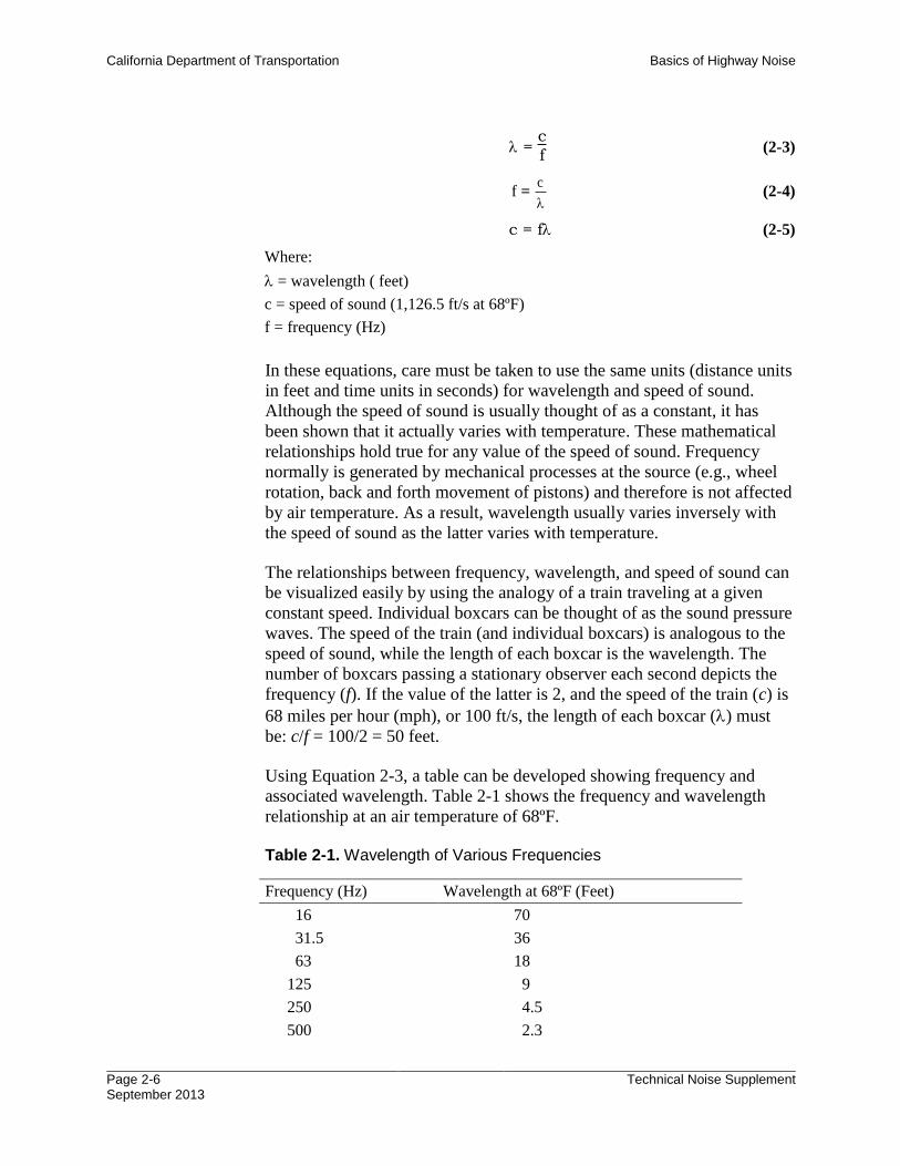
Using Equation 2-3, a table can be developed showing frequency and
associated wavelength. Table 2-1 shows the frequency and wavelength
relationship at an air temperature of 68ºF.
Table 2-1. Wavelength of Various Frequencies
Frequency (Hz) Wavelength at 68ºF (Feet)
16 70
31.5 36
63 18
125 9
250 4.5
500 2.3
California Department of Transportation Basics of Highway Noise
Technical Noise Supplement Page 2-7 September 2013
Frequency (Hz) Wavelength at 68ºF (Feet)
1,000 1.1
2,000 0.56
4,000 0.28
8,000 0.14
16,000 0.07
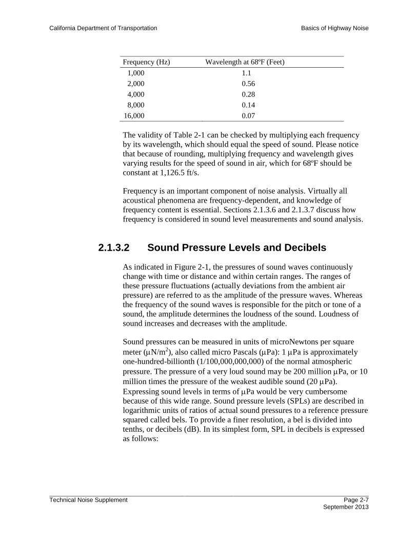
The validity of Table 2-1 can be checked by multiplying each frequency
by its wavelength, which should equal the speed of sound. Please notice
that because of rounding, multiplying frequency and wavelength gives
varying results for the speed of sound in air, which for 68ºF should be
constant at 1,126.5 ft/s.
Frequency is an important component of noise analysis. Virtually all
acoustical phenomena are frequency-dependent, and knowledge of
frequency content is essential. Sections 2.1.3.6 and 2.1.3.7 discuss how
frequency is considered in sound level measurements and sound analysis.
2.1.3.2 Sound Pressure Levels and Decibels
As indicated in Figure 2-1, the pressures of sound waves continuously
change with time or distance and within certain ranges. The ranges of
these pressure fluctuations (actually deviations from the ambient air
pressure) are referred to as the amplitude of the pressure waves. Whereas
the frequency of the sound waves is responsible for the pitch or tone of a
sound, the amplitude determines the loudness of the sound. Loudness of
sound increases and decreases with the amplitude.
Sound pressures can be measured in units of microNewtons per square
meter (N/m2), also called micro Pascals (Pa): 1 Pa is approximately
one-hundred-billionth (1/100,000,000,000) of the normal atmospheric
pressure. The pressure of a very loud sound may be 200 million Pa, or 10
million times the pressure of the weakest audible sound (20 Pa).
Expressing sound levels in terms of Pa would be very cumbersome
because of this wide range. Sound pressure levels (SPLs) are described in
logarithmic units of ratios of actual sound pressures to a reference pressure
squared called bels. To provide a finer resolution, a bel is divided into
tenths, or decibels (dB). In its simplest form, SPL in decibels is expressed
as follows:
California Department of Transportation Basics of Highway Noise
Page 2-8 September 2013
Technical Noise Supplement
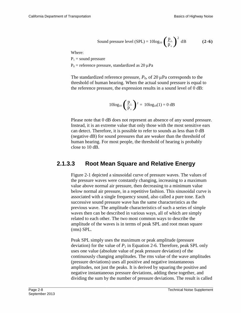
Sound pressure level (SPL) = 10log10 ( 1
0
p
p )2
dB (2-6)
Where:
P1 = sound pressure
P0 = reference pressure, standardized as 20 Pa
The standardized reference pressure, P0, of 20 Pa corresponds to the
threshold of human hearing. When the actual sound pressure is equal to
the reference pressure, the expression results in a sound level of 0 dB:
10log10 ( 1
0
p
p )2 = 10log10(1) = 0 dB
Please note that 0 dB does not represent an absence of any sound pressure.
Instead, it is an extreme value that only those with the most sensitive ears
can detect. Therefore, it is possible to refer to sounds as less than 0 dB
(negative dB) for sound pressures that are weaker than the threshold of
human hearing. For most people, the threshold of hearing is probably
close to 10 dB.
2.1.3.3 Root Mean Square and Relative Energy
Figure 2-1 depicted a sinusoidal curve of pressure waves. The values of
the pressure waves were constantly changing, increasing to a maximum
value above normal air pressure, then decreasing to a minimum value
below normal air pressure, in a repetitive fashion. This sinusoidal curve is
associated with a single frequency sound, also called a pure tone. Each
successive sound pressure wave has the same characteristics as the
previous wave. The amplitude characteristics of such a series of simple
waves then can be described in various ways, all of which are simply
related to each other. The two most common ways to describe the
amplitude of the waves is in terms of peak SPL and root mean square
(rms) SPL.
Peak SPL simply uses the maximum or peak amplitude (pressure
deviation) for the value of P1 in Equation 2-6. Therefore, peak SPL only
uses one value (absolute value of peak pressure deviation) of the
continuously changing amplitudes. The rms value of the wave amplitudes
(pressure deviations) uses all positive and negative instantaneous
amplitudes, not just the peaks. It is derived by squaring the positive and
negative instantaneous pressure deviations, adding these together, and
dividing the sum by the number of pressure deviations. The result is called
California Department of Transportation Basics of Highway Noise
Technical Noise Supplement Page 2-9 September 2013
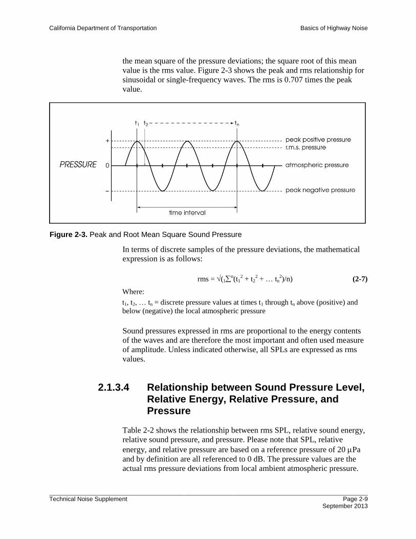
the mean square of the pressure deviations; the square root of this mean
value is the rms value. Figure 2-3 shows the peak and rms relationship for
sinusoidal or single-frequency waves. The rms is 0.707 times the peak
value.
In terms of discrete samples of the pressure deviations, the mathematical
expression is as follows:
rms = (1n(t1
2 + t2
2 + … tn
2)/n) (2-7)
Where:
t1, t2, … tn = discrete pressure values at times t1 through tn above (positive) and
below (negative) the local atmospheric pressure
Sound pressures expressed in rms are proportional to the energy contents
of the waves and are therefore the most important and often used measure
of amplitude. Unless indicated otherwise, all SPLs are expressed as rms
values.
2.1.3.4 Relationship between Sound Pressure Level, Relative Energy, Relative Pressure, and Pressure
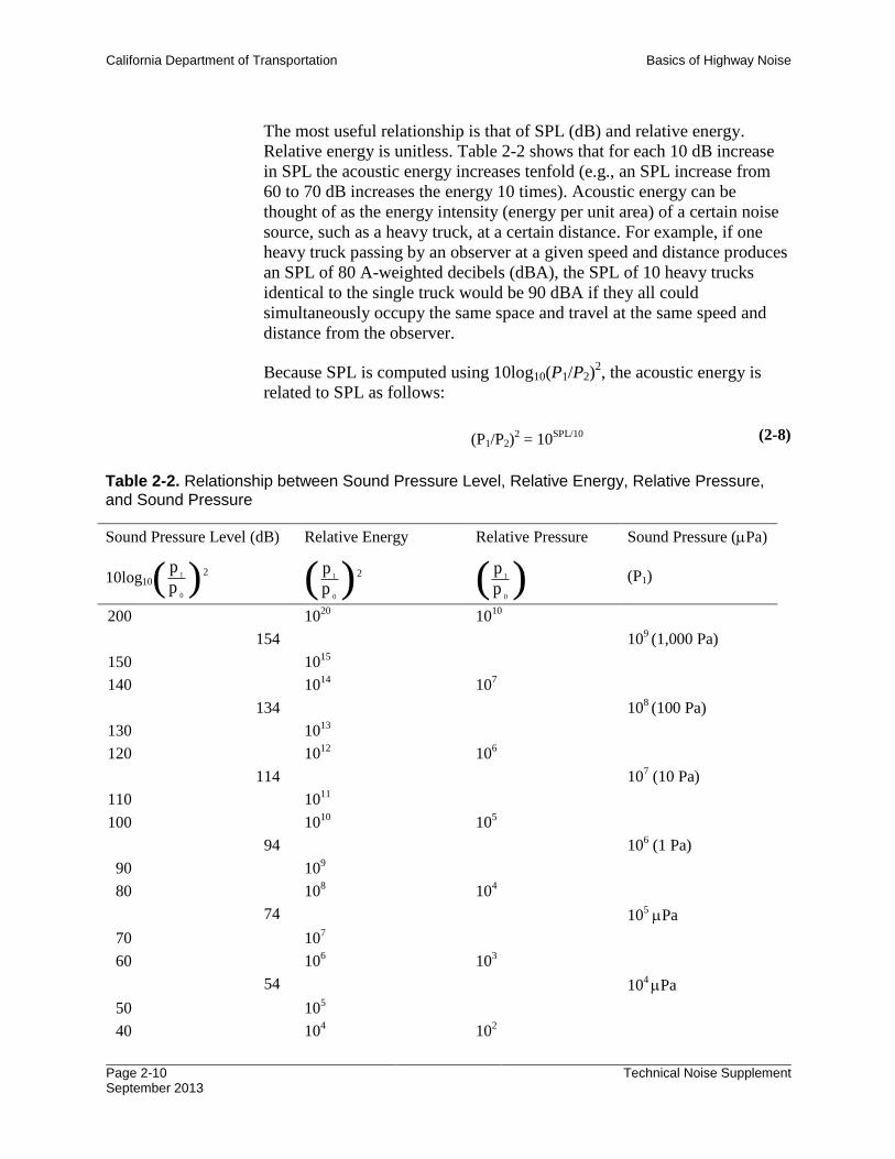
Table 2-2 shows the relationship between rms SPL, relative sound energy,
relative sound pressure, and pressure. Please note that SPL, relative
energy, and relative pressure are based on a reference pressure of 20 Pa
and by definition are all referenced to 0 dB. The pressure values are the
actual rms pressure deviations from local ambient atmospheric pressure.
Figure 2-3. Peak and Root Mean Square Sound Pressure
California Department of Transportation Basics of Highway Noise
Page 2-10 September 2013
Technical Noise Supplement
The most useful relationship is that of SPL (dB) and relative energy.
Relative energy is unitless. Table 2-2 shows that for each 10 dB increase
in SPL the acoustic energy increases tenfold (e.g., an SPL increase from
60 to 70 dB increases the energy 10 times). Acoustic energy can be
thought of as the energy intensity (energy per unit area) of a certain noise
source, such as a heavy truck, at a certain distance. For example, if one
heavy truck passing by an observer at a given speed and distance produces
an SPL of 80 A-weighted decibels (dBA), the SPL of 10 heavy trucks
identical to the single truck would be 90 dBA if they all could
simultaneously occupy the same space and travel at the same speed and
distance from the observer.
Because SPL is computed using 10log10(P1/P2)2, the acoustic energy is
related to SPL as follows:
(P1/P2)2 = 10
SPL/10 (2-8)
Table 2-2. Relationship between Sound Pressure Level, Relative Energy, Relative Pressure, and Sound Pressure
Sound Pressure Level (dB) Relative Energy Relative Pressure Sound Pressure (Pa)
10log10( 1
0
p
p )2 ( 1
0
p
p )2 ( 1
0
p
p ) (P1)
200 1020
1010
154 109 (1,000 Pa)
150 1015
140 1014
107
134 108 (100 Pa)
130 1013
120 1012
106
114 107 (10 Pa)
110 1011
100 1010
105
94 106 (1 Pa)
90 109
80 108 10
4
74 105 Pa
70 107
60 106 10
3
54 104 Pa
50 105
40 104 10
2
California Department of Transportation Basics of Highway Noise
Technical Noise Supplement Page 2-11 September 2013
Sound Pressure Level (dB) Relative Energy Relative Pressure Sound Pressure (Pa)
10log10( 1
0
p
p )2 ( 1
0
p
p )2 ( 1
0
p
p ) (P1)
34 103 Pa
30 103
20 102 10
1
14 102 Pa
10 101
0 100 = 1 = Ref. 10
0 = 1 = Ref. P1 = P0 = 20 Pa
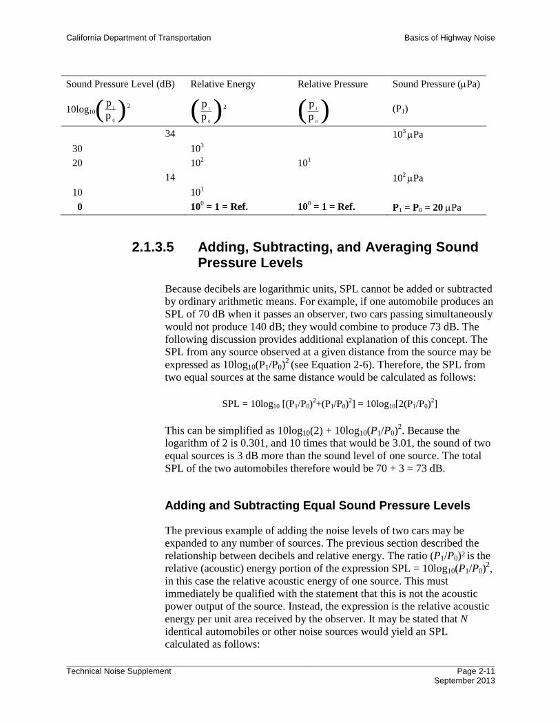
2.1.3.5 Adding, Subtracting, and Averaging Sound Pressure Levels
Because decibels are logarithmic units, SPL cannot be added or subtracted
by ordinary arithmetic means. For example, if one automobile produces an
SPL of 70 dB when it passes an observer, two cars passing simultaneously
would not produce 140 dB; they would combine to produce 73 dB. The
following discussion provides additional explanation of this concept. The
SPL from any source observed at a given distance from the source may be
expressed as 10log10(P1/P0)2 (see Equation 2-6). Therefore, the SPL from
two equal sources at the same distance would be calculated as follows:
SPL = 10log10 [(P1/P0)2+(P1/P0)
2] = 10log10[2(P1/P0)
2]
This can be simplified as 10log10(2) + 10log10(P1/P0)2. Because the
logarithm of 2 is 0.301, and 10 times that would be 3.01, the sound of two
equal sources is 3 dB more than the sound level of one source. The total
SPL of the two automobiles therefore would be 70 + 3 = 73 dB.
Adding and Subtracting Equal Sound Pressure Levels
The previous example of adding the noise levels of two cars may be
expanded to any number of sources. The previous section described the
relationship between decibels and relative energy. The ratio (P1/P0)2 is the
relative (acoustic) energy portion of the expression SPL = 10log10(P1/P0)2,
in this case the relative acoustic energy of one source. This must
immediately be qualified with the statement that this is not the acoustic
power output of the source. Instead, the expression is the relative acoustic
energy per unit area received by the observer. It may be stated that N
identical automobiles or other noise sources would yield an SPL
calculated as follows:
California Department of Transportation Basics of Highway Noise
Page 2-12 September 2013
Technical Noise Supplement
SPLTotal = SPL1 + 10log10(N) (2-9)
Where:
SPL1 = SPL of one source
N = number of identical sources to be added (must be more than 0)
Example
If one noise source produces 63 dB at a given distance, what would be the noise
level of 13 of the same source combined at the same distance?
Solution
SPLTotal = 63 + 10log10(13) = 63 + 11.1 = 74.1 dB
Equation 2-9 also may be rewritten as follows. This form is useful for
subtracting equal SPLs:
SPL1 = SPLTotal – 10log10(N) (2-10)
Example
The SPL of six equal sources combined is 68 dB at a given distance. What is the
noise level produced by one source?
Solution
SPL1 = 68 dB – 10log10(6) = 68 – 7.8 = 60.2 dB
In these examples, adding equal sources actually constituted multiplying
one source by the number of sources. Conversely, subtracting equal
sources was performed by dividing the total. For the latter, Equation 2-9
could have been written as SPL1 = SPLTotal + 10log10(1/N). The logarithm
of a fraction yields a negative result, so the answers would have been the
same.
These exercises are very useful for estimating traffic noise impacts. For
example, if one were to ask what the respective SPL increases would be
along a highway if existing traffic were doubled, tripled, or quadrupled
(assuming traffic mix, distribution, and speeds would not change), a
reasonable prediction could be made using Equation 2-9. In this case, N
would be the existing traffic (N = 1); N = 2 would be doubling, N = 3
would be tripling, and N = 4 would be quadrupling the existing traffic.
Because 10log10(N) in Equation 2-9 represents the increase in SPL, the
above values for N would yield +3, +4.8, and +6 dB, respectively.
Similarly, one might ask what the SPL decrease would be if traffic were
reduced by a factor of 2, 3, or 4 (i.e., N = 1/2, N = 1/3, and N = 1/4,
respectively). Applying 10log10(N) to these values would yield -3, -5, and
-6 dB, respectively.
California Department of Transportation Basics of Highway Noise
Technical Noise Supplement Page 2-13 September 2013
The same problem also may arise in a different form. For example, the
traffic flow on a given facility is 5,000 vehicles per hour, and the SPL is
65 dB at a given location next to the facility. One might ask what the
expected SPL would be if future traffic increased to 8,000 vehicles per
hour. The solution would be:
65 + 10log10(8,000/5,000) = 65 + 2 = 67 dB.
Therefore, N may represent an integer, fraction, or ratio. However, N
always must be more than 0. Taking the logarithm of 0 or a negative value
is not possible.
In Equations 2-9 and 2-10, 10log10(N) was the increase from SPL1 to
SPLTotal and equals the change in noise levels from an increase or decrease
in equal noise sources. Letting the change in SPLs be referred to as ΔSPL,
Equations 2-9 and 2-10 can be rewritten as follows:
ΔSPL = 10log10(N) (2-11)
This equation is useful for calculating the number of equal source
increments (N) that must be added or subtracted to change noise levels by
ΔSPL. For example, if it is known that an increase in traffic volumes
increases SPL by 7 dB, the factor change in traffic (assuming that traffic
mix and speeds did not change) can be calculated as follows:
7 dB = 10log10(N)
0.7 dB = log10(N)
100.7
= N
N = 5.0
Therefore, the traffic volume increased by a factor of 5.
Adding and Subtracting Unequal Sound Pressure Levels
If noise sources are not equal or equal noise sources are at different
distances, 10log10(N) cannot be used. Instead, SPLs must be added or
subtracted individually using the SPL and relative energy relationship in
Equation 2-8. If the number of SPLs to be added is N, and SPL1, SPL2,
and SPLn represent the first, second, and nth SPL, respectively, the
addition is accomplished as follows:
California Department of Transportation Basics of Highway Noise
Page 2-14 September 2013
Technical Noise Supplement
SPLTotal = 10log10[10SPL1/10
+ 10SPL2/10
+ … 10SPLn/10
] (2-12)
The above equation is the general equation for adding SPLs. The equation
also may be used for subtraction (simply change “+” to “–”). However, the
result between the brackets must always be more than 0. For example,
determining the total SPL of 82, 75, 88, 68, and 79 dB would use Equation
2-12 as follows:
SPL = 10log10 (10
68/10 + 10
75/10 + 10
79/10 + 10
82/10 + 10
88/10) = 89.6 dB
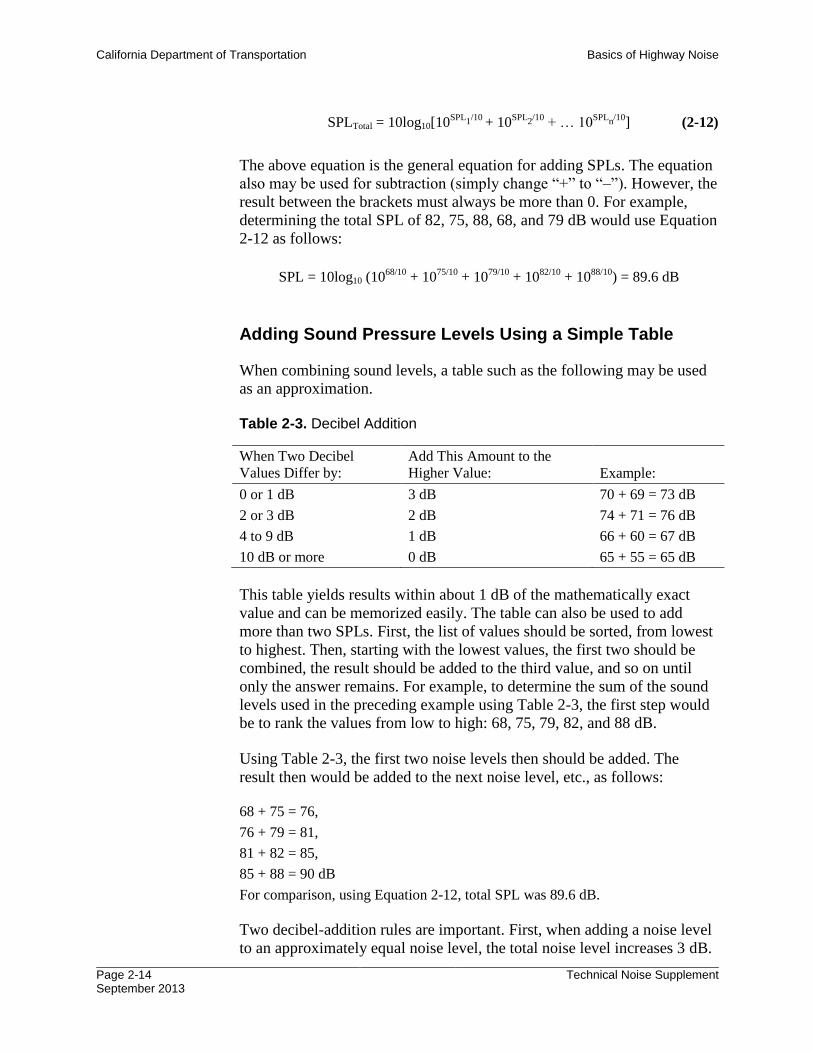
Adding Sound Pressure Levels Using a Simple Table
When combining sound levels, a table such as the following may be used
as an approximation.
Table 2-3. Decibel Addition
When Two Decibel
Values Differ by:
Add This Amount to the
Higher Value: Example:
0 or 1 dB 3 dB 70 + 69 = 73 dB
2 or 3 dB 2 dB 74 + 71 = 76 dB
4 to 9 dB 1 dB 66 + 60 = 67 dB
10 dB or more 0 dB 65 + 55 = 65 dB
This table yields results within about 1 dB of the mathematically exact
value and can be memorized easily. The table can also be used to add
more than two SPLs. First, the list of values should be sorted, from lowest
to highest. Then, starting with the lowest values, the first two should be
combined, the result should be added to the third value, and so on until
only the answer remains. For example, to determine the sum of the sound
levels used in the preceding example using Table 2-3, the first step would
be to rank the values from low to high: 68, 75, 79, 82, and 88 dB.
Using Table 2-3, the first two noise levels then should be added. The
result then would be added to the next noise level, etc., as follows:
68 + 75 = 76,
76 + 79 = 81,
81 + 82 = 85,
85 + 88 = 90 dB
For comparison, using Equation 2-12, total SPL was 89.6 dB.
Two decibel-addition rules are important. First, when adding a noise level
to an approximately equal noise level, the total noise level increases 3 dB.
California Department of Transportation Basics of Highway Noise
Technical Noise Supplement Page 2-15 September 2013
For example, doubling the traffic on a highway would result in an increase
of 3 dB. Conversely, reducing traffic by one half would reduce the noise
level by 3 dB. Second, when two noise levels are 10 dB or more apart, the
lower value does not contribute significantly (less than 0.5 dB) to the total
noise level. For example, 60 + 70 dB 70 dB. This means that if a noise
level measured from a source is at least 70 dB, the background noise level
(without the target source) must not be more than 60 dB to avoid risking
contamination.
Averaging Sound Pressure Levels
There are two ways of averaging SPLs: arithmetic averaging and energy-
averaging. Arithmetic averaging is simply averaging the decibel values.
For example, the arithmetic average (mean) of 60 and 70 dB is:
(60 + 70)/2 = 65 dB
Energy averaging is averaging of the energy values. Using the previous
example, the energy average (mean) of 60 and 70 dB is:
10log[(106.0
+ 107.0
)/2] = 67.4 dB
Please notice that the energy average is always equal to or more than the
arithmetic average. It is only equal to the arithmetic average if all values
are the same. Averaging the values 60, 60, 60, and 60 dB yields equal
results of 60 dB in both cases. The following discussion shows some
examples of when each method is appropriate.
Energy Averaging
Energy averaging is the most widely used method of averaging noise
levels. Sound energy relates directly to the sound source. For example, at a
given distance the sound energy from six equal noise sources is three
times that of two of the same sources at that same distance. To average the
number of sources and calculate the associated noise level, energy
averaging should be used. Examples of applications of energy averaging
are provided below.
Example 1
To determine the average noise level at a specific receiver along a
highway between 6 a.m. and 7 a.m., five 1-hour measurements were taken
on random days during that hour. The energy-averaged measurement
results were 68, 67, 71, 70, and 71 dB. What is a good estimate of the
noise level at that receiver? Because the main reason for the fluctuations in
noise levels is probably the differences in source strength (vehicle mix,
California Department of Transportation Basics of Highway Noise
Page 2-16 September 2013
Technical Noise Supplement
volumes, and speeds), energy averaging is appropriate. Therefore, the
result would be: 10log[(106.8
+ 106.7
+ 107.1
+ 107.0
+ 107.1
)/5] = 69.6 dB,
or 70 dB.
Example 2
Another situation is where traffic volumes substantially change during a
measurement period. Noise is measured at a location along a highway.
Vehicles on that highway are distributed equally, are traveling at the same
speed, and are of the same type (e.g., automobiles). Such traffic
characteristics would produce a near steady-state noise level. The typical
procedure would be to measure the traffic noise for an hour. After 15
minutes, the traffic volume suddenly increases sharply, but speeds remain
the same and the vehicles, although closer together, are still equally
distributed for the remaining 45 minutes. The noise level during the first
15 minutes was 70 dB and during the last 45 minutes was 75 dB. What
was the energy-averaged noise level? Because the time periods were not
the same, the energy average must be time-weighted by using the
following equation:
Energy-averaged noise level = 10log[(15 * 107.0
+ 45 * 107.5
)/60] = 74.2 dB
In this example, the time was weighted in units of minutes. This also could
have been accomplished using fractions of 1 hour, as follows:
Energy-averaged noise level = 10log[(0.25 * 107.0
+ 0.75 * 107.5
)/1] = 74.2 dB
Arithmetic Averaging
Arithmetic averaging is used less frequently, but it is used in situations
such as the following. For example, the objective is to measure the noise
of a machine with great accuracy. For simplicity, assume that the machine
produces a steady noise level, which is expected to be constant, each time
the machine is turned on. Because accuracy is of great importance, it is
chosen to take repeat measurements with different sound level meters and
to calculate the average noise level. In this case, it is appropriate to
calculate the arithmetic mean by adding the measured decibel values and
dividing by the number of measurements. Because the same source is
measured repeatedly, any measured noise fluctuations are mainly from
errors inherent in the instrumentation; method of measurement;
environmental conditions; and, to a certain extent, source strength.
Because the errors are distributed randomly, the expected value of the
measurements is the arithmetic mean.
It is also appropriate to use arithmetic means for statistical comparisons of
noise levels, or hypothesis testing, whether the noise levels were obtained
California Department of Transportation Basics of Highway Noise
Technical Noise Supplement Page 2-17 September 2013
by energy averaging or arithmetic means. Examples of applications of
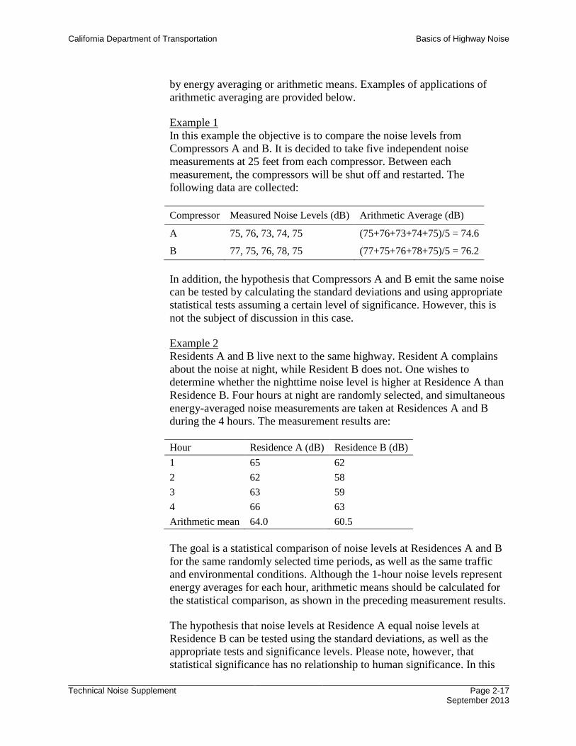
arithmetic averaging are provided below.
Example 1
In this example the objective is to compare the noise levels from
Compressors A and B. It is decided to take five independent noise
measurements at 25 feet from each compressor. Between each
measurement, the compressors will be shut off and restarted. The
following data are collected:
Compressor Measured Noise Levels (dB) Arithmetic Average (dB)
A 75, 76, 73, 74, 75 (75+76+73+74+75)/5 = 74.6
B 77, 75, 76, 78, 75 (77+75+76+78+75)/5 = 76.2
In addition, the hypothesis that Compressors A and B emit the same noise
can be tested by calculating the standard deviations and using appropriate
statistical tests assuming a certain level of significance. However, this is
not the subject of discussion in this case.
Example 2
Residents A and B live next to the same highway. Resident A complains
about the noise at night, while Resident B does not. One wishes to
determine whether the nighttime noise level is higher at Residence A than
Residence B. Four hours at night are randomly selected, and simultaneous
energy-averaged noise measurements are taken at Residences A and B
during the 4 hours. The measurement results are:
Hour Residence A (dB) Residence B (dB)
1 65 62
2 62 58
3 63 59
4 66 63
Arithmetic mean 64.0 60.5
The goal is a statistical comparison of noise levels at Residences A and B
for the same randomly selected time periods, as well as the same traffic
and environmental conditions. Although the 1-hour noise levels represent
energy averages for each hour, arithmetic means should be calculated for
the statistical comparison, as shown in the preceding measurement results.
The hypothesis that noise levels at Residence A equal noise levels at
Residence B can be tested using the standard deviations, as well as the
appropriate tests and significance levels. Please note, however, that
statistical significance has no relationship to human significance. In this
California Department of Transportation Basics of Highway Noise
Page 2-18 September 2013
Technical Noise Supplement
example, the noise level at Residence A is probably significantly higher
statistically than at Residence B. In terms of human perception, however,
the difference may be barely perceptible.
A good rule to remember is that whenever measurements or calculations
must relate to the number of sources or source strength, energy averaging
should be used. However, if improving accuracy in measurements or
calculations of the same events or making statistical comparisons is the
goal, the arithmetic mean is appropriate. Additional details about
averaging and time-weighting are addressed in Section 2.2.2.
2.1.3.6 A-Weighting and Noise Levels
SPL alone is not a reliable indicator of loudness. Frequency or pitch also
has a substantial effect on how humans respond. While the intensity
(energy per unit area) of the sound is a purely physical quantity, loudness
or human response depends on the characteristics of the human ear.
Human hearing is limited not only to the range of audible frequencies, but
also in the way it perceives the SPL in that range. In general, the healthy
human ear is most sensitive to sounds between 1,000 and 5,000 Hz and
perceives both higher and lower frequency sounds of the same magnitude
with less intensity. To approximate the frequency response of the human
ear, a series of SPL adjustments is usually applied to the sound measured
by a sound level meter. The adjustments, or weighting network, are
frequency-dependent.
The A-scale approximates the frequency response of the average young
ear when listening to most everyday sounds. When people make relative
judgments of the loudness or annoyance of a sound, their judgments
correlate well with the A-scale sound levels of those sounds. There are
other weighting networks that have been devised to address high noise
levels or other special problems (e.g., B-, C-, D-scales), but these scales
rarely, if ever, are used in conjunction with highway traffic noise. Noise
levels for traffic noise reports should be reported as dBA. In
environmental noise studies, A-weighted SPLs commonly are referred to
as noise levels.
Figure 2-4 shows the A-scale weighting network that is normally used to
approximate human response. The 0-dB line represents a reference line;
the curve represents frequency-dependent attenuations provided by the
ear’s response. Table 2-4 shows the standardized values (American
National Standards Institute 1983). The use of this weighting network is
signified by appending an “A” to the SPL as dBA or dB(A).
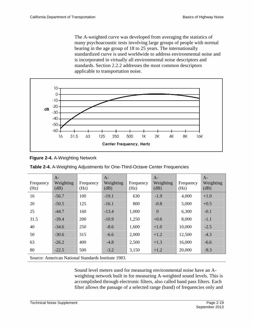
California Department of Transportation Basics of Highway Noise
Technical Noise Supplement Page 2-19 September 2013
The A-weighted curve was developed from averaging the statistics of
many psychoacoustic tests involving large groups of people with normal
hearing in the age group of 18 to 25 years. The internationally
standardized curve is used worldwide to address environmental noise and
is incorporated in virtually all environmental noise descriptors and
standards. Section 2.2.2 addresses the most common descriptors
applicable to transportation noise.
Table 2-4. A-Weighting Adjustments for One-Third-Octave Center Frequencies
Frequency
(Hz)
A-
Weighting
(dB)
Frequency
(Hz)
A-
Weighting
(dB)
Frequency
(Hz)
A-
Weighting
(dB)
Frequency
(Hz)
A-
Weighting
(dB)
16 -56.7 100 -19.1 630 -1.9 4,000 +1.0
20 -50.5 125 -16.1 800 -0.8 5,000 +0.5
25 -44.7 160 -13.4 1,000 0 6,300 -0.1
31.5 -39.4 200 -10.9 1,250 +0.6 8,000 -1.1
40 -34.6 250 -8.6 1,600 +1.0 10,000 -2.5
50 -30.6 315 -6.6 2,000 +1.2 12,500 -4.3
63 -26.2 400 -4.8 2,500 +1.3 16,000 -6.6
80 -22.5 500 -3.2 3,150 +1.2 20,000 -9.3
Source: American National Standards Institute 1983.
Sound level meters used for measuring environmental noise have an A-
weighting network built in for measuring A-weighted sound levels. This is
accomplished through electronic filters, also called band pass filters. Each
filter allows the passage of a selected range (band) of frequencies only and
Figure 2-4. A-Weighting Network
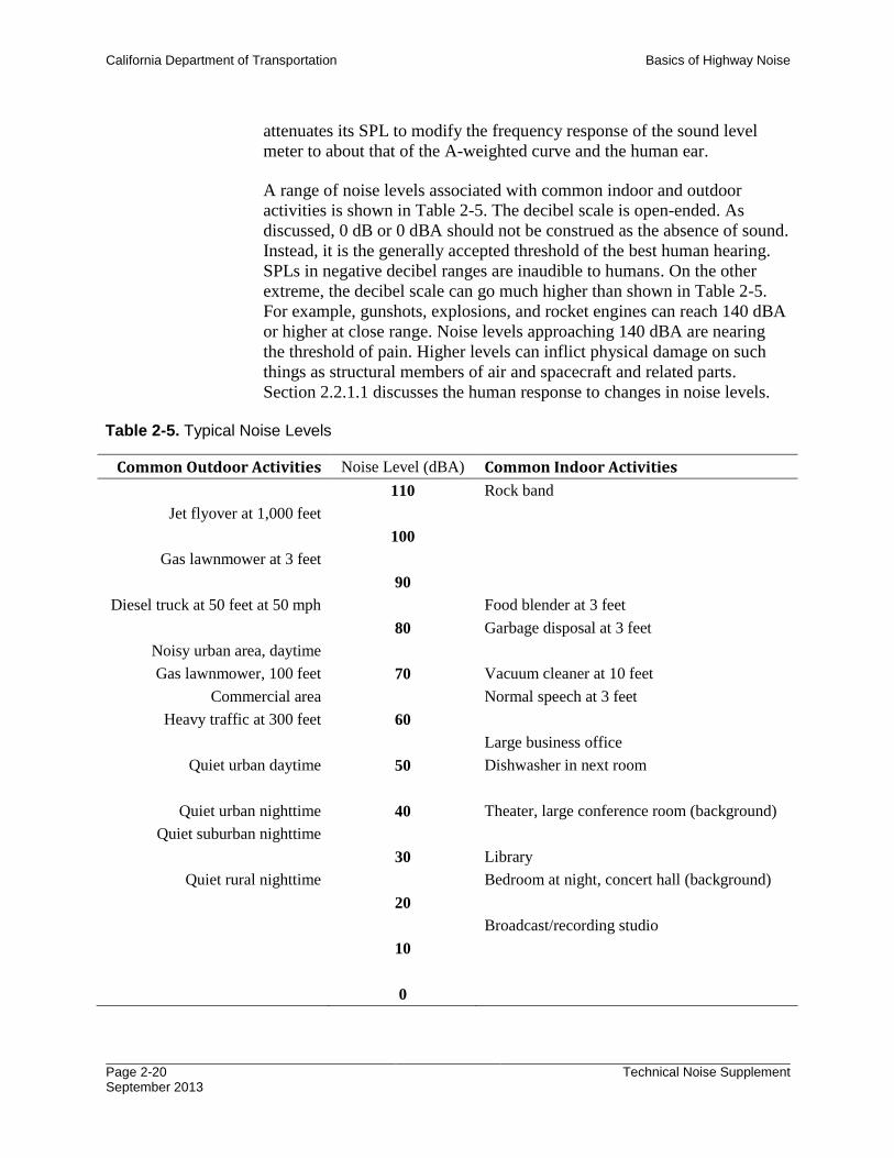
California Department of Transportation Basics of Highway Noise
Page 2-20 September 2013
Technical Noise Supplement
attenuates its SPL to modify the frequency response of the sound level
meter to about that of the A-weighted curve and the human ear.
A range of noise levels associated with common indoor and outdoor
activities is shown in Table 2-5. The decibel scale is open-ended. As
discussed, 0 dB or 0 dBA should not be construed as the absence of sound.
Instead, it is the generally accepted threshold of the best human hearing.
SPLs in negative decibel ranges are inaudible to humans. On the other
extreme, the decibel scale can go much higher than shown in Table 2-5.
For example, gunshots, explosions, and rocket engines can reach 140 dBA
or higher at close range. Noise levels approaching 140 dBA are nearing
the threshold of pain. Higher levels can inflict physical damage on such
things as structural members of air and spacecraft and related parts.
Section 2.2.1.1 discusses the human response to changes in noise levels.
Table 2-5. Typical Noise Levels
Common Outdoor Activities Noise Level (dBA) Common Indoor Activities
110 Rock band
Jet flyover at 1,000 feet
100
Gas lawnmower at 3 feet
90
Diesel truck at 50 feet at 50 mph Food blender at 3 feet
80 Garbage disposal at 3 feet
Noisy urban area, daytime
Gas lawnmower, 100 feet 70 Vacuum cleaner at 10 feet
Commercial area Normal speech at 3 feet
Heavy traffic at 300 feet 60
Large business office
Quiet urban daytime 50 Dishwasher in next room
Quiet urban nighttime 40 Theater, large conference room (background)
Quiet suburban nighttime
30 Library
Quiet rural nighttime Bedroom at night, concert hall (background)
20
Broadcast/recording studio
10
0
California Department of Transportation Basics of Highway Noise
Technical Noise Supplement Page 2-21 September 2013
2.1.3.7 Octave and One-Third-Octave Bands and Frequency Spectra
Very few sounds are pure tones (i.e., consisting of a single frequency). To
represent the complete characteristics of a sound properly, it is necessary
to divide the total sound into its frequency components (i.e., determine
how much sound [SPL] comes from each of the multiple frequencies that
make up the sound). This representation of frequency vs. SPL is called a
frequency spectrum. Spectra usually consist of 8- to 10-octave bands,
more or less spanning the frequency range of human hearing (20 to 20,000
Hz). Just as with a piano keyboard, an octave represents the frequency
interval between a given frequency and twice that frequency. Octave
bands are internationally standardized and identified by their “center
frequencies” (geometric means).
Because octave bands are rather broad, they are frequently subdivided into
thirds to create one-third-octave bands. These are also standardized. For
convenience, one-third-octave bands are sometimes numbered from 1
(1.25-Hz one-third-octave center frequency, which cannot be heard by
humans) to 43 (20,000-Hz one-third-octave center frequency). Within the
extreme range of human hearing there are 30 one-third-octave bands
ranging from band 13 (20-Hz one-third-octave center frequency) to band
42 (16,000-Hz one-third-octave center frequency). Table 2-6 shows the
ranges of the standardized octave and one-third-octave bands, as well as
band numbers.
Frequency spectra are used in many aspects of sound analysis, from
studying sound propagation to designing effective noise control measures.
Sound is affected by many frequency-dependent physical and
environmental factors. Atmospheric conditions, site characteristics, and
materials and their dimensions used for sound reduction are some of the
most important examples.
Sound propagating through the air is affected by air temperature,
humidity, wind and temperature gradients, vicinity and type of ground
surface, obstacles, and terrain features. These factors are all frequency-
dependent.
The ability of a material to transmit noise depends on the type of material
(concrete, wood, glass, etc.) and its thickness. Effectiveness of different
materials at transmitting noise depends on the frequency of the noise. See
Section 5.1.1 for a discussion of transmission loss and sound transmission
class.
Wavelengths serve to determine the effectiveness of noise barriers. Low
frequency noise, with its long wavelengths, passes easily around and over
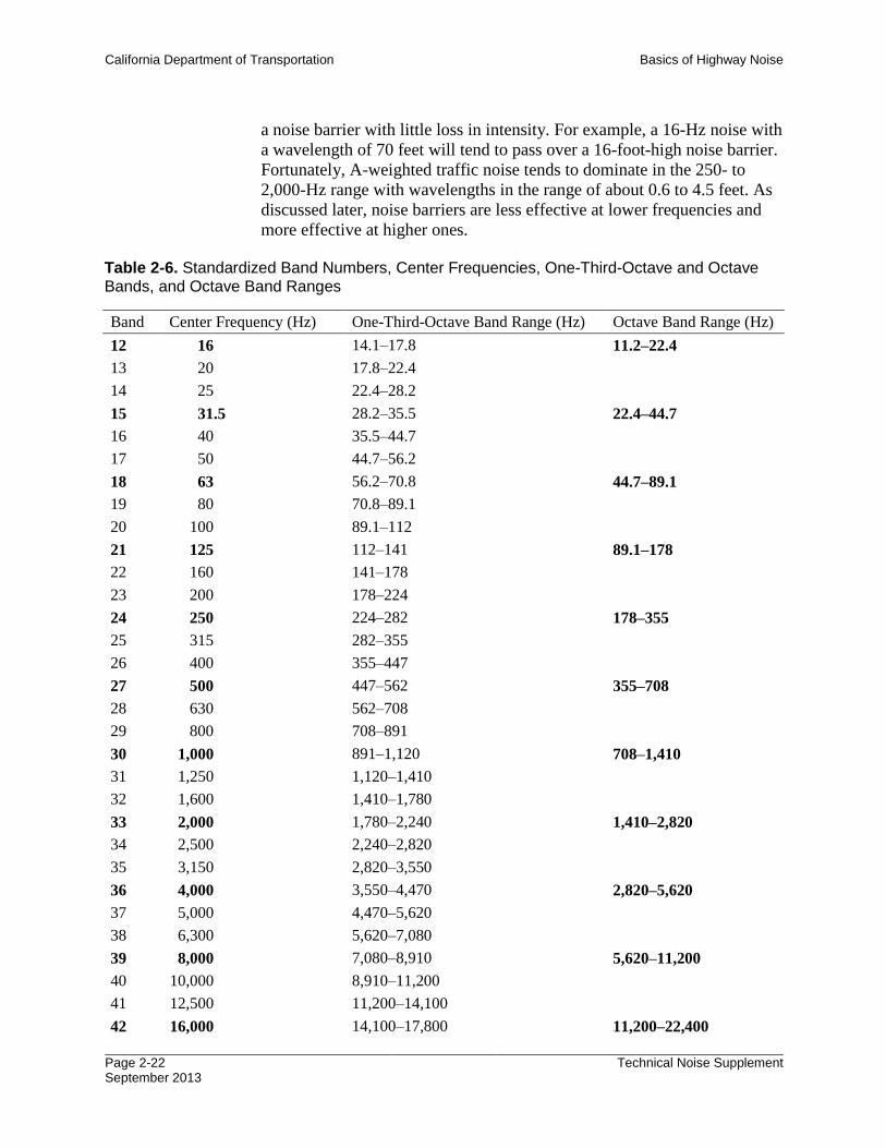
California Department of Transportation Basics of Highway Noise
Page 2-22 September 2013
Technical Noise Supplement
a noise barrier with little loss in intensity. For example, a 16-Hz noise with
a wavelength of 70 feet will tend to pass over a 16-foot-high noise barrier.
Fortunately, A-weighted traffic noise tends to dominate in the 250- to
2,000-Hz range with wavelengths in the range of about 0.6 to 4.5 feet. As
discussed later, noise barriers are less effective at lower frequencies and
more effective at higher ones.
Table 2-6. Standardized Band Numbers, Center Frequencies, One-Third-Octave and Octave Bands, and Octave Band Ranges
Band Center Frequency (Hz) One-Third-Octave Band Range (Hz) Octave Band Range (Hz)
12 16 14.1–17.8 11.2–22.4
13 20 17.8–22.4
14 25 22.4–28.2
15 31.5 28.2–35.5 22.4–44.7
16 40 35.5–44.7
17 50 44.7–56.2
18 63 56.2–70.8 44.7–89.1
19 80 70.8–89.1
20 100 89.1–112
21 125 112–141 89.1–178
22 160 141–178
23 200 178–224
24 250 224–282 178–355
25 315 282–355
26 400 355–447
27 500 447–562 355–708
28 630 562–708
29 800 708–891
30 1,000 891–1,120 708–1,410
31 1,250 1,120–1,410
32 1,600 1,410–1,780
33 2,000 1,780–2,240 1,410–2,820
34 2,500 2,240–2,820
35 3,150 2,820–3,550
36 4,000 3,550–4,470 2,820–5,620
37 5,000 4,470–5,620
38 6,300 5,620–7,080
39 8,000 7,080–8,910 5,620–11,200
40 10,000 8,910–11,200
41 12,500 11,200–14,100
42 16,000 14,100–17,800 11,200–22,400
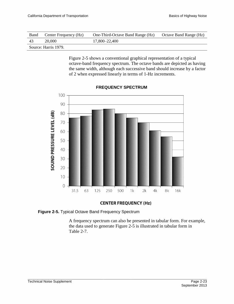
California Department of Transportation Basics of Highway Noise
Technical Noise Supplement Page 2-23 September 2013
Band Center Frequency (Hz) One-Third-Octave Band Range (Hz) Octave Band Range (Hz)
43 20,000 17,800–22,400
Source: Harris 1979.
Figure 2-5 shows a conventional graphical representation of a typical
octave-band frequency spectrum. The octave bands are depicted as having
the same width, although each successive band should increase by a factor
of 2 when expressed linearly in terms of 1-Hz increments.
A frequency spectrum can also be presented in tabular form. For example,
the data used to generate Figure 2-5 is illustrated in tabular form in
Table 2-7.
FREQUENCY SPECTRUM
Figure 2-5. Typical Octave Band Frequency Spectrum
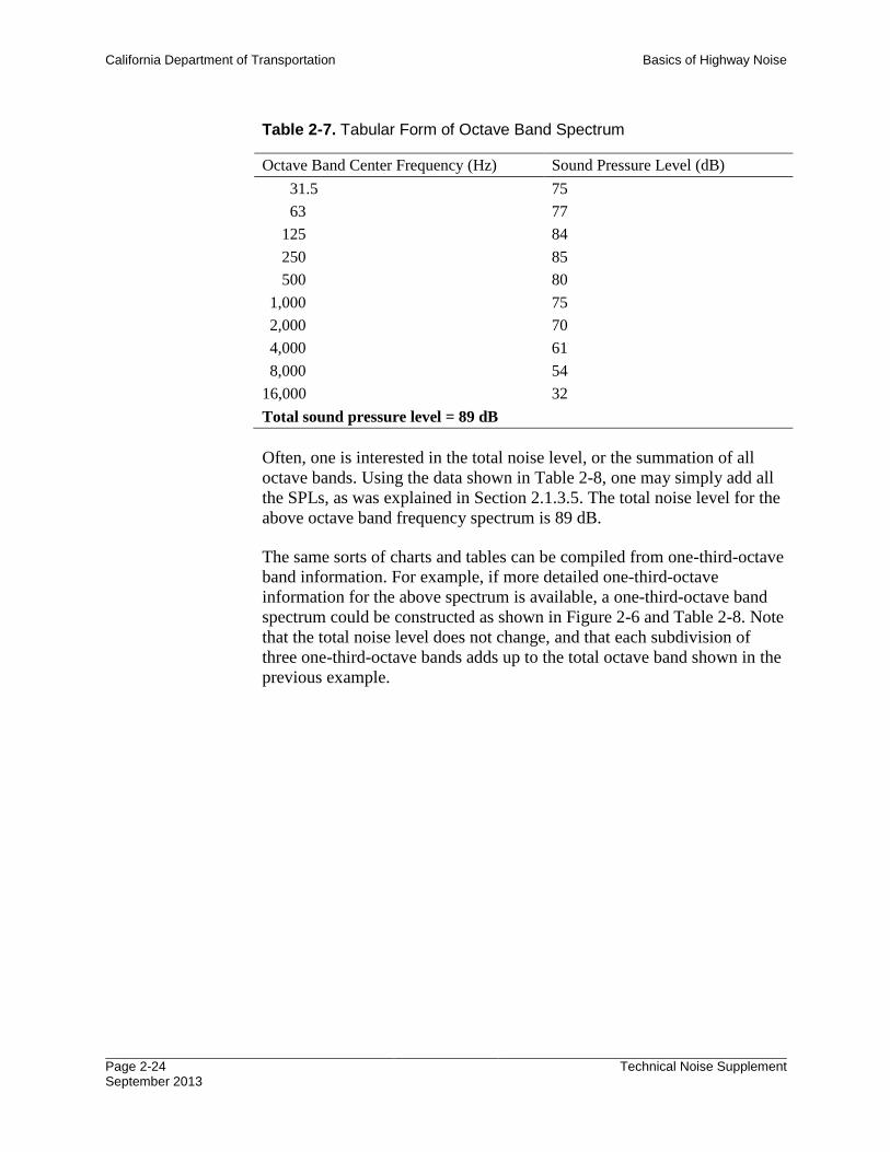
California Department of Transportation Basics of Highway Noise
Page 2-24 September 2013
Technical Noise Supplement
Table 2-7. Tabular Form of Octave Band Spectrum
Octave Band Center Frequency (Hz) Sound Pressure Level (dB)
31.5 75
63 77
125 84
250 85
500 80
1,000 75
2,000 70
4,000 61
8,000 54
16,000 32
Total sound pressure level = 89 dB
Often, one is interested in the total noise level, or the summation of all
octave bands. Using the data shown in Table 2-8, one may simply add all
the SPLs, as was explained in Section 2.1.3.5. The total noise level for the
above octave band frequency spectrum is 89 dB.
The same sorts of charts and tables can be compiled from one-third-octave
band information. For example, if more detailed one-third-octave
information for the above spectrum is available, a one-third-octave band
spectrum could be constructed as shown in Figure 2-6 and Table 2-8. Note
that the total noise level does not change, and that each subdivision of
three one-third-octave bands adds up to the total octave band shown in the
previous example.
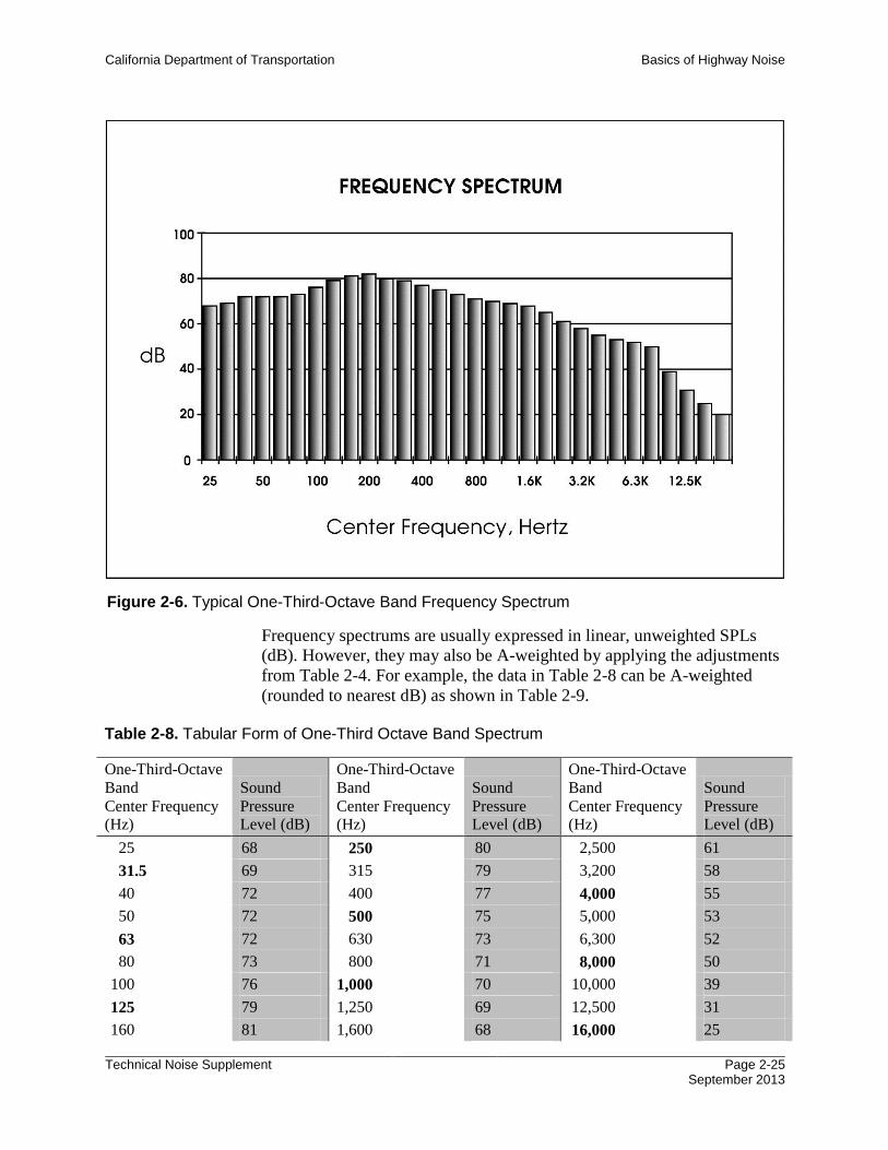
California Department of Transportation Basics of Highway Noise
Technical Noise Supplement Page 2-25 September 2013
Frequency spectrums are usually expressed in linear, unweighted SPLs
(dB). However, they may also be A-weighted by applying the adjustments
from Table 2-4. For example, the data in Table 2-8 can be A-weighted
(rounded to nearest dB) as shown in Table 2-9.
Table 2-8. Tabular Form of One-Third Octave Band Spectrum
One-Third-Octave
Band
Center Frequency (Hz)
Sound
Pressure Level (dB)
One-Third-Octave
Band
Center Frequency (Hz)
Sound
Pressure Level (dB)
One-Third-Octave
Band
Center Frequency (Hz)
Sound
Pressure Level (dB)
25 68 250 80 2,500 61
31.5 69 315 79 3,200 58
40 72 400 77 4,000 55
50 72 500 75 5,000 53
63 72 630 73 6,300 52
80 73 800 71 8,000 50
100 76 1,000 70 10,000 39
125 79 1,250 69 12,500 31
160 81 1,600 68 16,000 25
Figure 2-6. Typical One-Third-Octave Band Frequency Spectrum
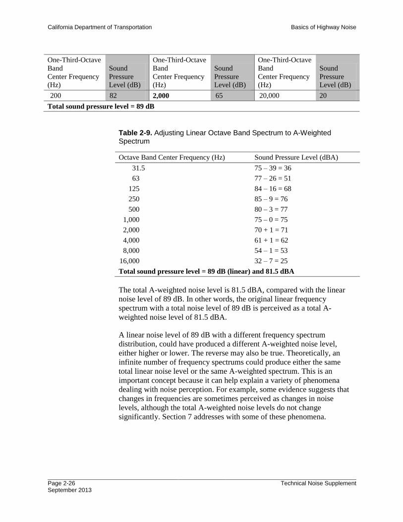
California Department of Transportation Basics of Highway Noise
Page 2-26 September 2013
Technical Noise Supplement
One-Third-Octave
Band
Center Frequency (Hz)
Sound
Pressure Level (dB)
One-Third-Octave
Band
Center Frequency (Hz)
Sound
Pressure Level (dB)
One-Third-Octave
Band
Center Frequency (Hz)
Sound
Pressure Level (dB)
200 82 2,000 65 20,000 20
Total sound pressure level = 89 dB
Table 2-9. Adjusting Linear Octave Band Spectrum to A-Weighted Spectrum
Octave Band Center Frequency (Hz) Sound Pressure Level (dBA)
31.5 75 – 39 = 36
63 77 – 26 = 51
125 84 – 16 = 68
250 85 – 9 = 76
500 80 – 3 = 77
1,000 75 – 0 = 75
2,000 70 + 1 = 71
4,000 61 + 1 = 62
8,000 54 – 1 = 53
16,000 32 – 7 = 25
Total sound pressure level = 89 dB (linear) and 81.5 dBA
The total A-weighted noise level is 81.5 dBA, compared with the linear
noise level of 89 dB. In other words, the original linear frequency
spectrum with a total noise level of 89 dB is perceived as a total A-
weighted noise level of 81.5 dBA.
A linear noise level of 89 dB with a different frequency spectrum
distribution, could have produced a different A-weighted noise level,
either higher or lower. The reverse may also be true. Theoretically, an
infinite number of frequency spectrums could produce either the same
total linear noise level or the same A-weighted spectrum. This is an
important concept because it can help explain a variety of phenomena
dealing with noise perception. For example, some evidence suggests that
changes in frequencies are sometimes perceived as changes in noise
levels, although the total A-weighted noise levels do not change
significantly. Section 7 addresses with some of these phenomena.
California Department of Transportation Basics of Highway Noise
Technical Noise Supplement Page 2-27 September 2013
2.1.3.8 White and Pink Noise
White noise is noise with a special frequency spectrum that has the same
amplitude (level) for each frequency interval over the entire audible
frequency spectrum. It is often generated in laboratories for calibrating
sound level measuring equipment, specifically its frequency response. One
might expect that the octave or one-third-octave band spectrum of white
noise would be a straight line, but this is not true. Beginning with the
lowest audible octave, each subsequent octave spans twice as many
frequencies than the previous ones, and therefore contains twice the
energy. This corresponds with a 3-dB step increase for each octave band,
and 1 dB for each one-third-octave band.
Pink noise, in contrast, is defined as having the same amplitude for each
octave band (or one-third-octave band), rather than for each frequency
interval. Its octave or one-third-octave band spectrum is truly a straight
“level” line over the entire audible spectrum. Therefore, pink noise
generators are conveniently used to calibrate octave or one-third-octave
band analyzers.
Both white and pink noise sound somewhat like the static heard from a
radio that is not tuned to a particular station.
2.1.4 Sound Propagation
From the source to receiver, noise changes both in level and frequency
spectrum. The most obvious is the decrease in noise as the distance from
the source increases. The manner in which noise reduces with distance
depends on the following important factors.
Geometric spreading from point and line sources.
Ground absorption.
Atmospheric effects and refraction.
Shielding by natural and manmade features, noise barriers, diffraction,
and reflection.
2.1.4.1 Geometric Spreading from Point and Line Sources
Sound from a small localized source (approximating a point source)
radiates uniformly outward as it travels away from the source in a
spherical pattern. The sound level attenuates or drops off at a rate of
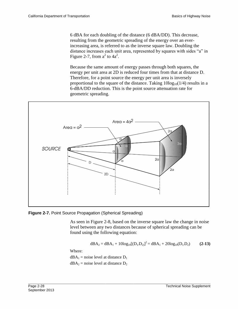
California Department of Transportation Basics of Highway Noise
Page 2-28 September 2013
Technical Noise Supplement
6 dBA for each doubling of the distance (6 dBA/DD). This decrease,
resulting from the geometric spreading of the energy over an ever-
increasing area, is referred to as the inverse square law. Doubling the
distance increases each unit area, represented by squares with sides “a” in
Figure 2-7, from a2 to 4a
2.
Because the same amount of energy passes through both squares, the
energy per unit area at 2D is reduced four times from that at distance D.
Therefore, for a point source the energy per unit area is inversely
proportional to the square of the distance. Taking 10log10(1/4) results in a
6-dBA/DD reduction. This is the point source attenuation rate for
geometric spreading.
As seen in Figure 2-8, based on the inverse square law the change in noise
level between any two distances because of spherical spreading can be
found using the following equation:
dBA2 = dBA1 + 10log10[(D1/D2)]2 = dBA1 + 20log10(D1/D2) (2-13)
Where:
dBA1 = noise level at distance D1
dBA2 = noise level at distance D2
Figure 2-7. Point Source Propagation (Spherical Spreading)
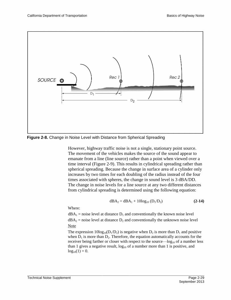
California Department of Transportation Basics of Highway Noise
Technical Noise Supplement Page 2-29 September 2013
However, highway traffic noise is not a single, stationary point source.
The movement of the vehicles makes the source of the sound appear to
emanate from a line (line source) rather than a point when viewed over a
time interval (Figure 2-9). This results in cylindrical spreading rather than
spherical spreading. Because the change in surface area of a cylinder only
increases by two times for each doubling of the radius instead of the four
times associated with spheres, the change in sound level is 3 dBA/DD.
The change in noise levels for a line source at any two different distances
from cylindrical spreading is determined using the following equation:
dBA2 = dBA1 + 10log10 (D1/D2) (2-14)
Where:
dBA1 = noise level at distance D1 and conventionally the known noise level
dBA2 = noise level at distance D2 and conventionally the unknown noise level
Note
The expression 10log10(D1/D2) is negative when D2 is more than D1 and positive
when D1 is more than D2. Therefore, the equation automatically accounts for the
receiver being farther or closer with respect to the source—log10 of a number less
than 1 gives a negative result, log10 of a number more than 1 is positive, and
log10(1) = 0.
Figure 2-8. Change in Noise Level with Distance from Spherical Spreading
Related Documents