STATE OF CALIFORNIA • DEPARTMENT OF TRANSPORTATION ADA Notice TECHNICAL REPORT DOCUMENTATION PAGE Forindividualswithsensorydisabilities,thisdocumentisavailableinalternate formats.Forinformationcall(916)654-6410orTDD(916)654-3880orwrite Records and TR0003 (REV 10/98) Lock Data on Form Forms Management, 1120 N Street, MS-89, Sacramento, CA 95814. 1.REPORT NUMBER 2.GOVERNMENT ASSOCIATION NUMBER 3. RECIPIENT'S CATALOG NUMBER CA17-2899 4. TITLE AND SUBTITLE 5. REPORT DATE Identify the Data Requirements for Safety Screening to Identify High February 15, 2018 Collision Concentration Locations 6.PERFORMING ORGANIZATION CODE 7.AUTHOR 8.PERFORMING ORGANIZATION REPORT NO. Aditya Medury, Bor-Wen Tsai, Offer Grembek, Venky Shankar, Norman Chao, Hassan Obeid, Hiram Gonzalez, and Praveen Vayalamkuzhi 9.PERFORMING ORGANIZATION NAME AND ADDRESS 10. WORK UNIT NUMBER UC Berkeley Safe Transportation Research & Education Center 2614 Dwight Way, #7374 11. CONTRACT OR GRANT NUMBER Berkeley, CA 94720-7374 65A0574 13. TYPE OF REPORT AND PERIOD COVERED 12. SPONSORING AGENCY AND ADDRESS California Department of Transportation Final Report Division of Research and Innovation and System Information, MS-83 14. SPONSORING AGENCY CODE 1727 30 th Street Sacramento CA 95816 15. SUPPLEMENTARY NOTES 16. ABSTRACT An integral component of identifying high collision concentration locations (HCCLs) through network screening techniques are safety performance functions (SPFs), which are mathematical equations that relate collision frequencies (of different types) to traffic volumes at a given location and other site characteristics such as, road geometry, intersection design, etc. There are two types of SPFs, referred to as Type 1 (that use only traffic volumes) and Type 2 (that use traffic volumes as well as other site characteristics). Parallel efforts within Caltrans to develop California-specific Type 1 and Type 2 SPFs have revealed that the data currently available in Caltrans for SPF development suffer from limitations. The first is the absence of data with regards to some attributes (e.g., horizontal and vertical alignment); and the second is the inconsistent quality of the available data. The objective of this research project was to (a) identify additional data sources bother within and outside of Caltrans that can be utilized for collecting new data elements for SPF modeling, and (b) evaluate the suitability of existing data sources that are currently being used for SPF development. The research team identified automated pavement condition survey data, Google Street View/Earth and HERE Maps and Google Elevation API as potential data sources for estimating new roadway design/operational variables that can improve the quality of SPFs. In addition, a suitability analysis framework was also proposed which evaluates the quality of a data element through the metrics of completeness, frequency of updates and spatial variation. Finally, a roadmap for which variables are suitable for SPF modeling and recommendations for how these variables need to be collected were provided. 17. KEY WORDS safety performance function, model transferability, roadway segments, intersections, ramps 17. DISTRIBUTION STATEMENT No restrictions. This document is available to the public through the National Technical Information Service, Springfield, VA 22161 19. SECURITY CLASSIFICATION(of this report) Unclassified 20.NUMBER OF PAGES 129 21.COST OF REPORT CHARGED N/A Reproduction of completed page authorized.

Welcome message from author
This document is posted to help you gain knowledge. Please leave a comment to let me know what you think about it! Share it to your friends and learn new things together.
Transcript
STATE OF CALIFORNIA • DEPARTMENT OF TRANSPORTATION ADA Notice TECHNICAL REPORT DOCUMENTATION PAGE Forindividualswithsensorydisabilities,thisdocumentisavailableinalternate formats.Forinformationcall(916)654-6410orTDD(916)654-3880orwrite Records and TR0003 (REV 10/98) Lock Data on Form Forms Management, 1120 N Street, MS-89, Sacramento, CA 95814.
1.REPORT NUMBER 2.GOVERNMENT ASSOCIATION NUMBER 3. RECIPIENT'S CATALOG NUMBER
CA17-2899 4. TITLE AND SUBTITLE 5. REPORT DATE
Identify the Data Requirements for Safety Screening to Identify High February 15, 2018 Collision Concentration Locations
6.PERFORMING ORGANIZATION CODE
7.AUTHOR 8.PERFORMING ORGANIZATION REPORT NO.
Aditya Medury, Bor-Wen Tsai, Offer Grembek, Venky Shankar, Norman Chao, Hassan Obeid, Hiram Gonzalez, and Praveen Vayalamkuzhi 9.PERFORMING ORGANIZATION NAME AND ADDRESS 10. WORK UNIT NUMBER
UC Berkeley Safe Transportation Research & Education Center 2614 Dwight Way, #7374 11. CONTRACT OR GRANT NUMBER
Berkeley, CA 94720-7374 65A0574 13. TYPE OF REPORT AND PERIOD COVERED 12. SPONSORING AGENCY AND ADDRESS
California Department of Transportation Final Report Division of Research and Innovation and System Information, MS-83
14. SPONSORING AGENCY CODE 1727 30thStreet Sacramento CA 95816
15. SUPPLEMENTARY NOTES
16. ABSTRACT
An integral component of identifying high collision concentration locations (HCCLs) through network screening techniques are safety performance functions (SPFs), which are mathematical equations that relate collision frequencies (of different types) to traffic volumes at a given location and other site characteristics such as, road geometry, intersection design, etc. There are two types of SPFs, referred to as Type 1 (that use only traffic volumes) and Type 2 (that use traffic volumes as well as other site characteristics). Parallel efforts within Caltrans to develop California-specific Type 1 and Type 2 SPFs have revealed that the data currently available in Caltrans for SPF development suffer from limitations. The first is the absence of data with regards to some attributes (e.g., horizontal and vertical alignment); and the second is the inconsistent quality of the available data. The objective of this research project was to (a) identify additional data sources bother within and outside of Caltrans that can be utilized for collecting new data elements for SPF modeling, and (b) evaluate the suitability of existing data sources that are currently being used for SPF development. The research team identified automated pavement condition survey data, Google Street View/Earth and HERE Maps and Google Elevation API as potential data sources for estimating new roadway design/operational variables that can improve the quality of SPFs. In addition, a suitability analysis framework was also proposed which evaluates the quality of a data element through the metrics of completeness, frequency of updates and spatial variation. Finally, a roadmap for which variables are suitable for SPF modeling and recommendations for how these variables need to be collected were provided.
17. KEY WORDS
safety performance function, model transferability, roadway segments, intersections, ramps
17. DISTRIBUTION STATEMENT
No restrictions. This document is available to the public through the National Technical Information Service, Springfield, VA 22161
19. SECURITY CLASSIFICATION(of this report)
Unclassified
20.NUMBER OF PAGES
129
21.COST OF REPORT CHARGED
N/A
Reproduction of completed page authorized.
DISCLAIMER STATEMENT
This document is disseminated in the interest of information exchange. The contents of this report reflect the views of the authors who are responsible for the facts and accuracy of the data presented herein. The contents do not necessarily reflect the official views or policies of the State of California or the Federal Highway Administration. This publication does not constitute a standard, specification or regulation. This report does not constitute an endorsement by the Department of any product described herein.
For individuals with sensory disabilities, this document is available in Braille, large print, audiocassette, or compact disk. To obtain a copy of this document in one of these alternate formats, please contact: the Division of Research and Innovation, MS-83 California Department of Transportation, P.O. Box 942873, Sacramento, CA 94273-0001

IDENTIFY THE DATA REQUIREMENTS FOR SAFETY SCREENING TO IDENTIFY
HIGH COLLISION CONCENTRATION LOCATIONS
FINAL TECHNICAL REPORT
ADITYA MEDURY BOR-WEN TSAI
OFFER GREMBEK VENKY SHANKAR NORMAN CHAO HASSAN OBEID
HIRAM GONZALEZ PRAVEEN VAYALAMKUZHI
PREPARED BY THE UC BERKELEY SAFE TRANSPORTATION RESEARCH AND EDUCATION CENTER
FOR THE CALIFORNIA DEPARTMENT OF TRANSPORTATION
FEBRUARY 15, 2018
ii
ACKNOWLEDGEMENTS
The authors would like to thank the California Department of Transportation for their support of this project. We especially acknowledge the support, guidance, and collaboration of John Ensch, Eric Wong, Brian Domsic, Vladimir Poroshin, Hau Doan, ShiriedelAcayan, Aaron Truong, and Matthew Friedmanat Caltrans. We would also like to acknowledge the inputs provided by Timothy Lim at the University of California, Berkeley, and Scott Mathison at Pathway Services, Inc. We also deeply appreciate thework of Jerry Kwong of the Division of Research and Innovation for facilitating the project from its inception and through the final report.
iii
TABLE OF CONTENTS
EXECUTIVE SUMMARY ........................................................................................................................ 1
1. INTRODUCTION.............................................................................................................................. 3
1.1. Motivation and Goals.....................................................................................................3 1.2. Key Components...........................................................................................................4
2. IDENTIFICATION OF DESIRABLE DATA ELEMENTS FOR SPF DEVELOPMENT........ 6
2.1. Summary of existing SPF model development .............................................................6 2.2. Identification of desirable data elements .......................................................................7
3. POTENTIAL DATA SOURCES WITHIN CALTRANS............................................................... 9
3.1. TASAS...........................................................................................................................9 3.2. Traffic Census Program ..............................................................................................13 3.3. Pavement Management ..............................................................................................13 3.4. Photolog ......................................................................................................................15 3.5. Districts........................................................................................................................15
4. SUITABILITY ANALYSIS OF EXISTING DATA SOURCES WITHIN CALTRANS.......... 16
4.1. Methodological framework ..........................................................................................16 4.1.1. Proposed metrics ................................................................................................16 4.1.2. Outlier analysis ....................................................................................................17
4.2. Analysis of data sources within Caltrans.....................................................................17 4.2.1. TASAS.................................................................................................................17 4.2.2. Truck Volumes ....................................................................................................35 4.2.3. Horizontal and Vertical Alignment Data from Pathway........................................37
5. POTENTIAL DATA SOURCES OUTSIDE OF CALTRANS.................................................... 40
5.1. Horizontal Alignment Estimation using GIS.................................................................40 5.1.1. Texas DOT’s GIS Tool ........................................................................................40 5.1.2. Nevada DOT’s GIS Tool: CATER Curvature.......................................................41
5.2. Posted Speed Limit (HERE Maps API) .......................................................................42 5.3. Elevation Data for Vertical Alignment using Google Elevation API/R .........................44
5.3.1. Algorithm that Determines Point of Vertical Intersection .....................................45 5.4. Google Street View .....................................................................................................45 5.5. Google Earth ...............................................................................................................46
6. PILOT STUDY FOR DATA COLLECTION USING EXTERNAL SOURCES....................... 47
6.1. Sampling methodology for pilot locations....................................................................47 6.2. List of locations for the pilot study ...............................................................................48 6.3. Data collection preparation..........................................................................................49
6.3.1. Customization for Google Earth ..........................................................................49 6.3.2. Infrastructure Data Collection Macro...................................................................51 6.3.3. Manual data collection protocol for individual variables ......................................52
iv
7. PILOT RESULTS ............................................................................................................................ 63
7.1. Summary statistics of variables collected across different projects ............................63 7.2. Time-cost estimation ...................................................................................................63 7.3. Analysis of specific variables.......................................................................................64
7.3.1. Differences observed between TASAS and manually collected crosswalk locations 64 7.3.2. Ground truth comparisons...................................................................................65
8. ROBUSTNESS ANALYSIS OF ELEVATION VARIABLE....................................................... 74
8.1. How Elevation Noise Affects Grade/Grade Difference................................................74 8.2. How Station Interval Affects Piecewise Regression Results.......................................77 8.3. Determination of Appropriate Categories for Grade Differences.................................78 8.4. PVI Identification Error and PVI Redistribution Error...................................................83 8.5. Grade Difference Analysis: Robustness of Category ..................................................90 8.6. Concluding Remarks ...................................................................................................93
9. COMPARISON BETWEEN PATHWAY AND GIS-BASED TOOLS FOR CURVATURE ESTIMATION........................................................................................................................................... 96
9.1. 9.1. Pathway Dataset ..................................................................................................96 9.2. GIS-based Horizontal Curvature Tool Requirements..................................................96 9.3. Preliminary comparison of curve estimation based on SR 160 sample data ..............97 9.4. Recommended definitions of alignment-related variables...........................................98
10. CONCLUSION AND RECOMMENDATIONS ......................................................................... 101
10.1. Summary of results ...................................................................................................101 10.2. Recommendation for new and existing variables for SPF modeling .........................103
APPENDIX A. DEFINITIONS OF DESIRABLE SPF VARIABLES............................................... 113
A.1. Segments ......................................................................................................................113 A.2. Intersections ..................................................................................................................118 A.3. Ramps ...........................................................................................................................120
v

EXECUTIVE SUMMARY
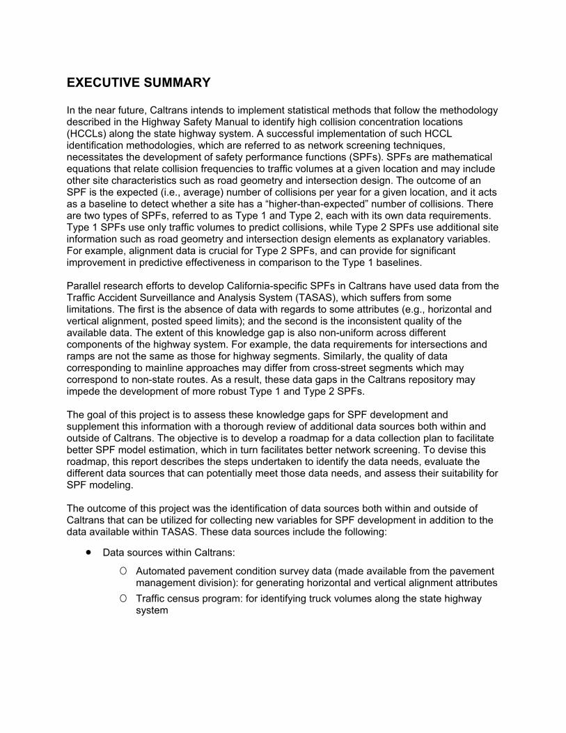
In the near future, Caltrans intends to implement statistical methods that follow the methodology described in the Highway Safety Manual to identify high collision concentration locations (HCCLs) along the state highway system. A successful implementation of such HCCL identification methodologies, which are referred to as network screening techniques, necessitates the development of safety performance functions (SPFs). SPFs are mathematical equations that relate collision frequencies to traffic volumes at a given location and may include other site characteristics such as road geometry and intersection design. The outcome of an SPF is the expected (i.e., average) number of collisions per year for a given location, and it acts as a baseline to detect whether a site has a “higher-than-expected” number of collisions. There are two types of SPFs, referred to as Type 1 and Type 2, each with its own data requirements. Type 1 SPFs use only traffic volumes to predict collisions, while Type 2 SPFs use additional site information such as road geometry and intersection design elements as explanatory variables. For example, alignment data is crucial for Type 2 SPFs, and can provide for significant improvement in predictive effectiveness in comparison to the Type 1 baselines.
Parallel research efforts to develop California-specific SPFs in Caltrans have used data from the Traffic Accident Surveillance and Analysis System (TASAS), which suffers from some limitations. The first is the absence of data with regards to some attributes (e.g., horizontal and vertical alignment, posted speed limits); and the second is the inconsistent quality of the available data. The extent of this knowledge gap is also non-uniform across different components of the highway system. For example, the data requirements for intersections and ramps are not the same as those for highway segments. Similarly, the quality of data corresponding to mainline approaches may differ from cross-street segments which may correspond to non-state routes. As a result, these data gaps in the Caltrans repository may impede the development of more robust Type 1 and Type 2 SPFs.
The goal of this project is to assess these knowledge gaps for SPF development and supplement this information with a thorough review of additional data sources both within and outside of Caltrans. The objective is to develop a roadmap for a data collection plan to facilitate better SPF model estimation, which in turn facilitates better network screening. To devise this roadmap, this report describes the steps undertaken to identify the data needs, evaluate the different data sources that can potentially meet those data needs, and assess their suitability for SPF modeling.
The outcome of this project was the identification of data sources both within and outside of Caltrans that can be utilized for collecting new variables for SPF development in addition to the data available within TASAS. These data sources include the following:
• Data sources within Caltrans:
O Automated pavement condition survey data (made available from the pavement management division): for generating horizontal and vertical alignment attributes
O Traffic census program: for identifying truck volumes along the state highway system
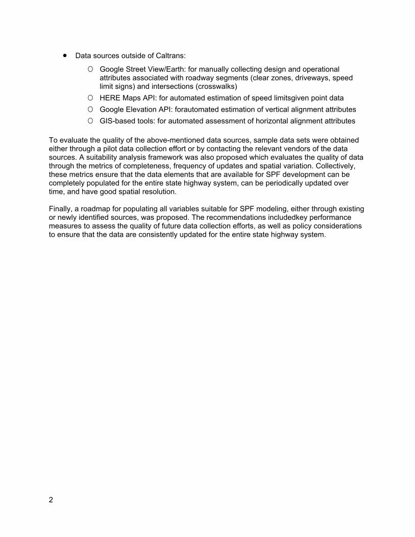
• Data sources outside of Caltrans:
O Google Street View/Earth: for manually collecting design and operational attributes associated with roadway segments (clear zones, driveways, speed limit signs) and intersections (crosswalks)
O HERE Maps API: for automated estimation of speed limitsgiven point data O Google Elevation API: forautomated estimation of vertical alignment attributes O GIS-based tools: for automated assessment of horizontal alignment attributes
To evaluate the quality of the above-mentioned data sources, sample data sets were obtained either through a pilot data collection effort or by contacting the relevant vendors of the data sources. A suitability analysis framework was also proposed which evaluates the quality of data through the metrics of completeness, frequency of updates and spatial variation. Collectively, these metrics ensure that the data elements that are available for SPF development can be completely populated for the entire state highway system, can be periodically updated over time, and have good spatial resolution.
Finally, a roadmap for populating all variables suitable for SPF modeling, either through existing or newly identified sources, was proposed. The recommendations includedkey performance measures to assess the quality of future data collection efforts, as well as policy considerations to ensure that the data are consistently updated for the entire state highway system.
2
1. INTRODUCTION
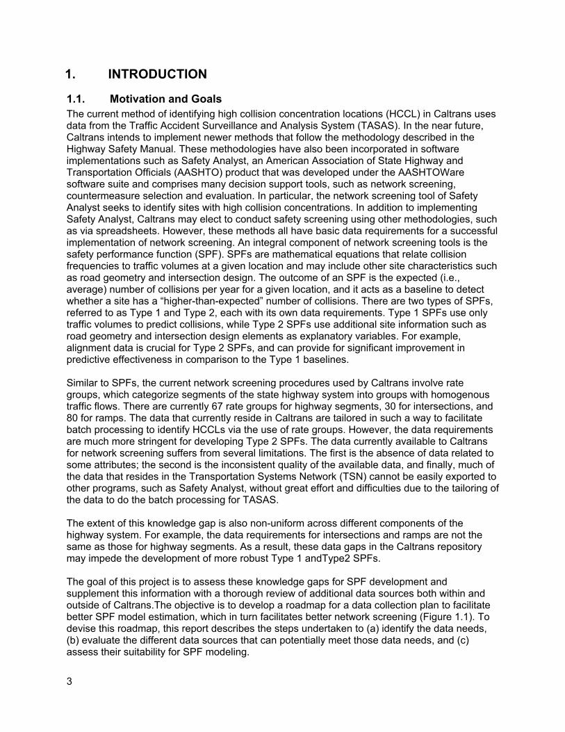
1.1. Motivation and Goals The current method of identifying high collision concentration locations (HCCL) in Caltrans uses data from the Traffic Accident Surveillance and Analysis System (TASAS). In the near future, Caltrans intends to implement newer methods that follow the methodology described in the Highway Safety Manual. These methodologies have also been incorporated in software implementations such as Safety Analyst, an American Association of State Highway and Transportation Officials (AASHTO) product that was developed under the AASHTOWare software suite and comprises many decision support tools, such as network screening, countermeasure selection and evaluation. In particular, the network screening tool of Safety Analyst seeks to identify sites with high collision concentrations. In addition to implementing Safety Analyst, Caltrans may elect to conduct safety screening using other methodologies, such as via spreadsheets. However, these methods all have basic data requirements for a successful implementation of network screening. An integral component of network screening tools is the safety performance function (SPF). SPFs are mathematical equations that relate collision frequencies to traffic volumes at a given location and may include other site characteristics such as road geometry and intersection design. The outcome of an SPF is the expected (i.e., average) number of collisions per year for a given location, and it acts as a baseline to detect whether a site has a “higher-than-expected” number of collisions. There are two types of SPFs, referred to as Type 1 and Type 2, each with its own data requirements. Type 1 SPFs use only traffic volumes to predict collisions, while Type 2 SPFs use additional site information such as road geometry and intersection design elements as explanatory variables. For example, alignment data is crucial for Type 2 SPFs, and can provide for significant improvement in predictive effectiveness in comparison to the Type 1 baselines.
Similar to SPFs, the current network screening procedures used by Caltrans involve rate groups, which categorize segments of the state highway system into groups with homogenous traffic flows. There are currently 67 rate groups for highway segments, 30 for intersections, and 80 for ramps. The data that currently reside in Caltrans are tailored in such a way to facilitate batch processing to identify HCCLs via the use of rate groups. However, the data requirements are much more stringent for developing Type 2 SPFs. The data currently available to Caltrans for network screening suffers from several limitations. The first is the absence of data related to some attributes; the second is the inconsistent quality of the available data, and finally, much of the data that resides in the Transportation Systems Network (TSN) cannot be easily exported to other programs, such as Safety Analyst, without great effort and difficulties due to the tailoring of the data to do the batch processing for TASAS.
The extent of this knowledge gap is also non-uniform across different components of the highway system. For example, the data requirements for intersections and ramps are not the same as those for highway segments. As a result, these data gaps in the Caltrans repository may impede the development of more robust Type 1 andType2 SPFs.
The goal of this project is to assess these knowledge gaps for SPF development and supplement this information with a thorough review of additional data sources both within and outside of Caltrans.The objective is to develop a roadmap for a data collection plan to facilitate better SPF model estimation, which in turn facilitates better network screening (Figure 1.1). To devise this roadmap, this report describes the steps undertaken to (a) identify the data needs, (b) evaluate the different data sources that can potentially meet those data needs, and (c) assess their suitability for SPF modeling.
3
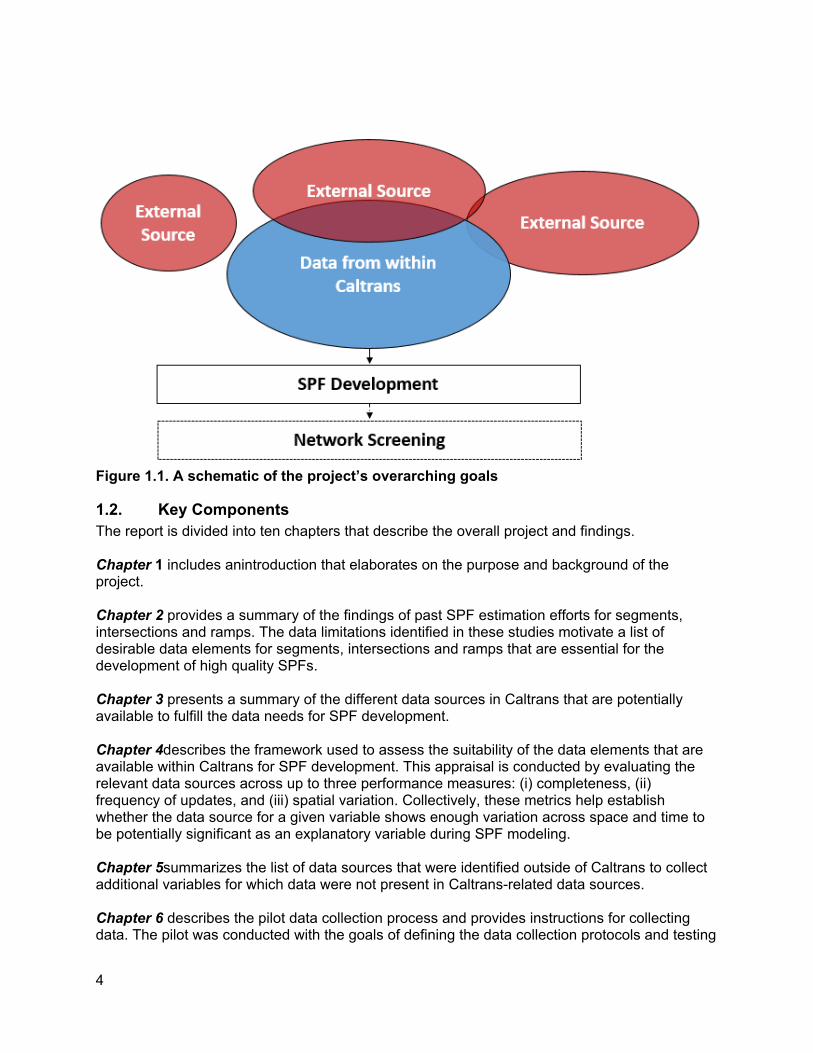
Figure 1.1. A schematic of the project’s overarching goals
1.2. Key Components The report is divided into ten chapters that describe the overall project and findings.
Chapter 1 includes anintroduction that elaborates on the purpose and background of the project.
Chapter 2 provides a summary of the findings of past SPF estimation efforts for segments, intersections and ramps. The data limitations identified in these studies motivate a list of desirable data elements for segments, intersections and ramps that are essential for the development of high quality SPFs.
Chapter 3 presents a summary of the different data sources in Caltrans that are potentially available to fulfill the data needs for SPF development.
Chapter 4describes the framework used to assess the suitability of the data elements that are available within Caltrans for SPF development. This appraisal is conducted by evaluating the relevant data sources across up to three performance measures: (i) completeness, (ii) frequency of updates, and (iii) spatial variation. Collectively, these metrics help establish whether the data source for a given variable shows enough variation across space and time to be potentially significant as an explanatory variable during SPF modeling.
Chapter 5summarizes the list of data sources that were identified outside of Caltrans to collect additional variables for which data were not present in Caltrans-related data sources.
Chapter 6 describes the pilot data collection process and provides instructions for collecting data. The pilot was conducted with the goals of defining the data collection protocols and testing
4

them across a wide variety of road conditions. The pilot study sought to estimate the total time required to collect data across the entire state highway network, primarily using aerial and street view imagery. In addition, the pilot also served the purpose of obtaining ground truth to compare the performance of automated, scalable data sources.
Chapter 7provides estimates of the time required to collect the relevant variables across the entire California state highway network. In addition, the data collection effort helped identify several inconsistencies among the Caltrans sources, as well as to assist in comparing the accuracies of scalable data collection approaches for elevation and posted speed limits using ground truth collected from the pilot study.
Chapter 8 discusses the robustness analysis to help identify a suitable variable definition for the vertical alignment-related variable to better address potential noise in the quality of elevation data.
Chapter 9 conducts an exploratory comparison between horizontal curvature data obtained from automated pavement condition surveys and GIS-based road curvature estimation tools
Finally, Chapter 10 synthesizes the study outcomes to present a roadmap of the variables that can be used for SPF modeling, and how they can be collected for the entire state highway system moving forward.
5
2. IDENTIFICATION OF DESIRABLE DATA ELEMENTS FOR SPF DEVELOPMENT
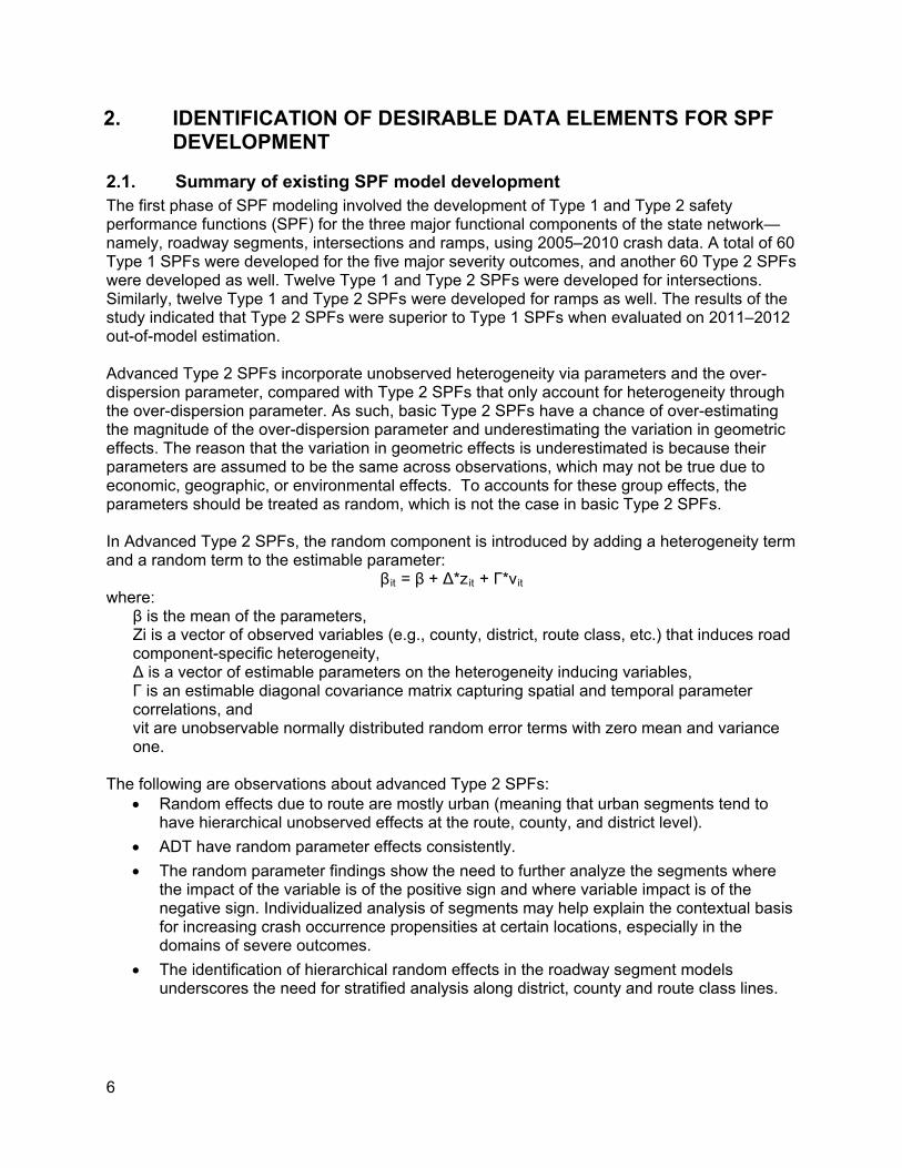
2.1. Summary of existing SPF model development The first phase of SPF modeling involved the development of Type 1 and Type 2 safety performance functions (SPF) for the three major functional components of the state network— namely, roadway segments, intersections and ramps, using 2005–2010 crash data. A total of 60 Type 1 SPFs were developed for the five major severity outcomes, and another 60 Type 2 SPFs were developed as well. Twelve Type 1 and Type 2 SPFs were developed for intersections. Similarly, twelve Type 1 and Type 2 SPFs were developed for ramps as well. The results of the study indicated that Type 2 SPFs were superior to Type 1 SPFs when evaluated on 2011–2012 out-of-model estimation.
Advanced Type 2 SPFs incorporate unobserved heterogeneity via parameters and the over-dispersion parameter, compared with Type 2 SPFs that only account for heterogeneity through the over-dispersion parameter. As such, basic Type 2 SPFs have a chance of over-estimating the magnitude of the over-dispersion parameter and underestimating the variation in geometric effects. The reason that the variation in geometric effects is underestimated is because their parameters are assumed to be the same across observations, which may not be true due to economic, geographic, or environmental effects. To accounts for these group effects, the parameters should be treated as random, which is not the case in basic Type 2 SPFs.
In Advanced Type 2 SPFs, the random component is introduced by adding a heterogeneity term and a random term to the estimable parameter:
βit = β + Δ*zit + Γ*νit where:
β is the mean of the parameters, Zi is a vector of observed variables (e.g., county, district, route class, etc.) that induces road component-specific heterogeneity, Δ is a vector of estimable parameters on the heterogeneity inducing variables, Γ is an estimable diagonal covariance matrix capturing spatial and temporal parameter correlations, and νit are unobservable normally distributed random error terms with zero mean and variance one.
The following are observations about advanced Type 2 SPFs: • Random effects due to route are mostly urban (meaning that urban segments tend to
have hierarchical unobserved effects at the route, county, and district level). • ADT have random parameter effects consistently. • The random parameter findings show the need to further analyze the segments where
the impact of the variable is of the positive sign and where variable impact is of the negative sign. Individualized analysis of segments may help explain the contextual basis for increasing crash occurrence propensities at certain locations, especially in the domains of severe outcomes.
• The identification of hierarchical random effects in the roadway segment models underscores the need for stratified analysis along district, county and route class lines.
6

The SPF modeling process also revealed that missing data may contribute to overdispersion in the models due to heterogeneity that arises from the missing geometric data. Examples of missing variables include:
• Alignment data, cross-street geometry (minor street geometry, and when available, the resolution is not the same as the mainline), horizontal and vertical curvature data (which leads to curvature variables not being evaluated).
• Incomplete data such as missing AADT or missing lane information. • Cross street crash history is not available (so only mainline crashes are studied). • Length of ramps, their geometry, and ramp alignment information.
2.2. Identification of desirable data elements Prior to initiating the identification of data sources that can fill in the specific data gaps listed below, it is important to formalize the list of variables that are desirable for SPF modeling. The following sections outline the variables identified to be essential in SPF development for segments, intersections and ramps. These variables include both available as well as missing variables.
Segments • Location information: starting and ending post miles • Design speeds (design speeds are preferred to posted speed limits, as posted speed
limits do not adequately reflect the design speed considerations, especially on lower functional classes)
• Lane information: number of through lanes, lane widths, shoulder widths, lane type such as auxiliary lanes, , center left turn lanes
• Roadside information: clear zones, fixed objects, roadside rating, median type • Traffic information: annual average daily traffic (AADT) estimate, including truck traffic • Horizontal alignment: horizontal curve degree or radius,curve super elevation, length of
curve, location of points of curvature and tangency, superelevation-runoff data, and central angle
• Vertical alignment: point of vertical curvature, point of vertical tangent stations and elevations of these points, point of vertical intersection station and elevation information, rate of vertical curvature information, length of vertical curve, as well as initial and final grade of curve (for cases in which horizontal and vertical curves overlap)
Intersections • Location information: post miles (location identifier) including post miles of cross streets
where applicable • Traffic control type: signalized or unsignalized • Type of signal phasing: two-phase versus multi-phase • Intersection geometry:
o Roadway information about the approaching and exiting highway segments, as well as the cross streets, using the inventory described in the roadway segment description.
o Additional intersection-specific geometry elements include auxiliary lanes (such as turning lanes), roadside barriers, channelization, curb treatments, crosswalk type.
7

• Speed limits: of all approaching and exiting roadway segments. (If speed limits are not posted on approaches, inferred design speeds based on alignment geometry may be required.)
• AADT information: of all approaching and exiting roadway segments (including turning movements)
Ramps • Location information: post miles (location identifier) • Ramp configuration: loop versus directional (interchange type) • Ramp lengths • Horizontal alignment • Vertical alignment • Ramp metering information • Roadway features at beginning and ending ramp terminal
In the following chapter, the list of data sources that are available in Caltrans are be discussed, with an emphasis of determining the variables listed above within those databases.
8

3. POTENTIAL DATA SOURCES WITHIN CALTRANS
3.1. TASAS The Traffic Accident Surveillance and Analysis System (TASAS) database, which includes information on California’s state highway system including infrastructure (e.g., number of lanes, lane widths, etc.), vehicular volumes, and crashes, is the primary data source in Caltrans for conducting traffic safety-related analysis. For the purposes of this project, the emphasis is exclusively on the infrastructure database, although for the SPF development, the crash database is be needed.
The TASAS infrastructure database contains information about segments, intersections, and ramps. This database is jointly maintained by Caltrans headquarters and individual district offices. To analyze the attributes of the TASAS database, a clean road file containing historical TASAS records for segments, intersections and ramps from 2008 onward was obtained.
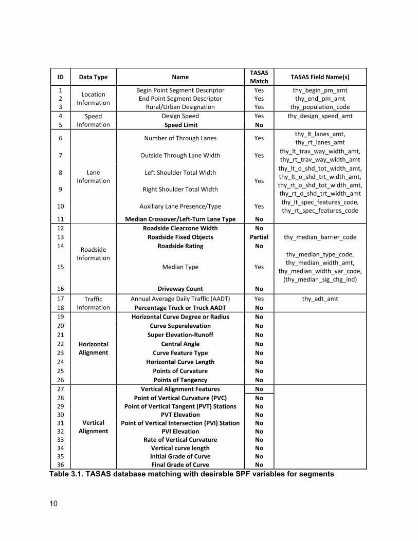
Regarding the desirable SPF input variables listed in Chapter 2, Tables 3.1-3.3 list the data elements in TASAS that were identified to be desirable for SPF modeling. A data dictionary defining the desirable SPF variables is provided in Appendix A.
As Table 3.1 indicates, the significant data elements that are missing from TASAS segment database are:
• Horizontal alignment • Vertical alignment • Speed limits • Specific lane information types (center left turn lane and driveways) • Specific roadside information (clear zones) • Truck volumes
It is important to note that the different geometric variables listed in Table 3.1 represent different aspects of horizontal and vertical profile. It ispossible thatall these variables may not besimultaneously included within an SPF model, as some of them may be correlated with each other. However, having access to the different attributes of horizontal and vertical alignment can help identify which variables would be most significant forType 2 SPFs during the estimation process.
9
ID Data Type Name TASAS Match TASAS Field Name(s)
1 2 3
Location Information
Begin Point Segment Descriptor End Point Segment Descriptor
Rural/Urban Designation
Yes Yes Yes
thy_begin_pm_amt thy_end_pm_amt
thy_population_code 4 5
Speed Information
Design Speed Speed Limit
Yes No
thy_design_speed_amt
6 Number of Through Lanes Yes thy_lt_lanes_amt, thy_rt_lanes_amt
7 Outside Through Lane Width Yes thy_lt_trav_way_width_amt, thy_rt_trav_way_width_amt
8
9
Lane Information
Left Shoulder Total Width
Right Shoulder Total Width Yes
thy_lt_o_shd_tot_width_amt, thy_lt_o_shd_trt_width_amt, thy_rt_o_shd_tot_width_amt, thy_rt_o_shd_trt_width_amt
10 Auxiliary Lane Presence/Type Yes thy_lt_spec_features_code, thy_rt_spec_features_code
11 Median Crossover/Left-Turn Lane Type No 12 Roadside Clearzone Width No 13 Roadside Fixed Objects Partial thy_median_barrier_code 14
15
Roadside Information
Roadside Rating
Median Type
No
Yes
thy_median_type_code, thy_median_width_amt,
thy_median_width_var_code, (thy_median_sig_chg_ind)
16 Driveway Count No 17 18
Traffic Information
Annual Average Daily Traffic (AADT) Percentage Truck or Truck AADT
Yes No
thy_adt_amt
19 Horizontal Curve Degree or Radius No 20 Curve Superelevation No 21 Super Elevation-Runoff No 22 Horizontal Central Angle No 23 Alignment Curve Feature Type No 24 Horizontal Curve Length No 25 Points of Curvature No 26 Points of Tangency No 27 28
Vertical Alignment Features Point of Vertical Curvature (PVC)
No No
29 Point of Vertical Tangent (PVT) Stations No 30 PVT Elevation No 31 Vertical Point of Vertical Intersection (PVI) Station No 32 Alignment PVI Elevation No 33 Rate of Vertical Curvature No 34 Vertical curve length No 35 Initial Grade of Curve No 36 Final Grade of Curve No
Table 3.1. TASAS database matching with desirable SPF variables for segments
10
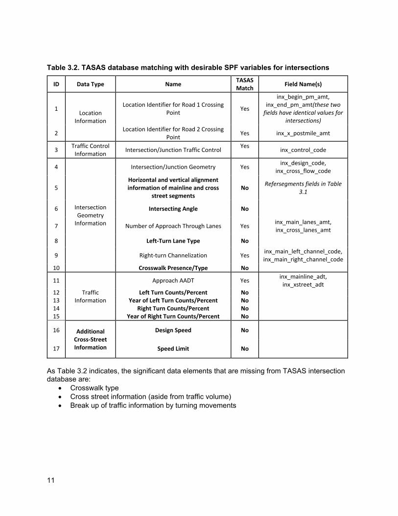
Table 3.2. TASAS database matching with desirable SPF variables for intersections
ID Data Type Name TASAS Match Field Name(s)
inx_begin_pm_amt,
1 Location
Information
Location Identifier for Road 1 Crossing Point Yes inx_end_pm_amt(these two
fields have identical values for intersections)
2 Location Identifier for Road 2 Crossing Point Yes inx_x_postmile_amt
3 Traffic Control Information Intersection/Junction Traffic Control Yes inx_control_code
4 Intersection/Junction Geometry Yes inx_design_code, inx_cross_flow_code
5 Horizontal and vertical alignment information of mainline and cross
street segments No Refersegments fields in Table
3.1
6 Intersection Geometry
Intersecting Angle No
7 Information Number of Approach Through Lanes Yes inx_main_lanes_amt, inx_cross_lanes_amt
8 Left-Turn Lane Type No
9 Right-turn Channelization Yes inx_main_left_channel_code, inx_main_right_channel_code
10 Crosswalk Presence/Type No
11 Approach AADT Yes inx_mainline_adt, inx_xstreet_adt
12 Traffic Left Turn Counts/Percent No 13 Information Year of Left Turn Counts/Percent No 14 Right Turn Counts/Percent No 15 Year of Right Turn Counts/Percent No
16
17
Additional Cross-Street Information
Design Speed
Speed Limit
No
No
As Table 3.2 indicates, the significant data elements that are missing from TASAS intersection database are:
• Crosswalk type • Cross street information (aside from traffic volume) • Break up of traffic information by turning movements
11
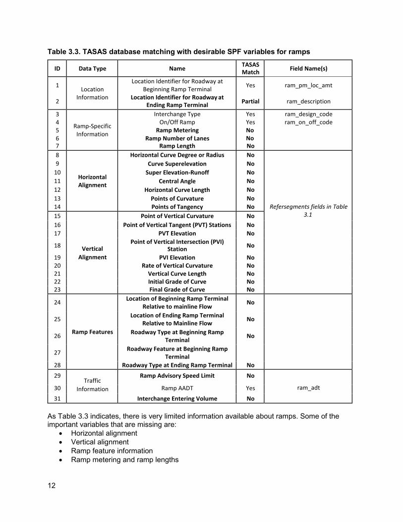
Table 3.3. TASAS database matching with desirable SPF variables for ramps
ID Data Type Name TASAS Match Field Name(s)
1
2
Location
Information
Location Identifier for Roadway at Beginning Ramp Terminal
Location Identifier for Roadway at Ending Ramp Terminal
Yes
Partial
ram_pm_loc_amt
ram_description
3 4 5 6 7
Ramp-Specific Information
Interchange Type On/Off Ramp
Ramp Metering Ramp Number of Lanes
Ramp Length
Yes Yes No No No
ram_design_code ram_on_off_code
8 9
10 11 12 13 14
Horizontal Alignment
Horizontal Curve Degree or Radius Curve Superelevation
Super Elevation-Runoff Central Angle
Horizontal Curve Length Points of Curvature Points of Tangency
No No No No No No No
Refersegments fields in Table 3.1 15 Point of Vertical Curvature No
16 Point of Vertical Tangent (PVT) Stations No 17 PVT Elevation No
18
Vertical Point of Vertical Intersection (PVI)
Station No
19 Alignment PVI Elevation No 20 Rate of Vertical Curvature No 21 Vertical Curve Length No 22 Initial Grade of Curve No 23 Final Grade of Curve No
24
Ramp Features
Location of Beginning Ramp Terminal Relative to mainline Flow
No
25 Location of Ending Ramp Terminal Relative to Mainline Flow No
26 Roadway Type at Beginning Ramp Terminal No
27 Roadway Feature at Beginning Ramp Terminal
28 Roadway Type at Ending Ramp Terminal No
29 Traffic
Ramp Advisory Speed Limit No
ram_adt 30 Information Ramp AADT Yes
31 Interchange Entering Volume No As Table 3.3 indicates, there is very limited information available about ramps. Some of the important variables that are missing are:
• Horizontal alignment • Vertical alignment • Ramp feature information • Ramp metering and ramp lengths
12
For the desirable variables for which TASAS matching data elements are available, subsequent analysis is required to assess their suitability, which is the focus of section 4.2.1.
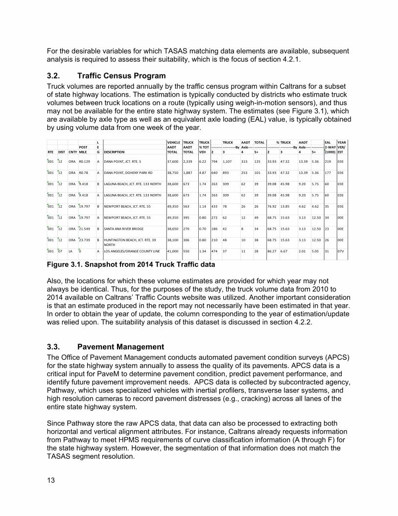
3.2. Traffic Census Program Truck volumes are reported annually by the traffic census program within Caltrans for a subset of state highway locations. The estimation is typically conducted by districts who estimate truck volumes between truck locations on a route (typically using weigh-in-motion sensors), and thus may not be available for the entire state highway system. The estimates (see Figure 3.1), which are available by axle type as well as an equivalent axle loading (EAL) value, is typically obtained by using volume data from one week of the year.
L VEHICLE TRUCK TRUCK TRUCK AADT TOTAL % TRUCK AADT EAL YEAR POST E AADT AADT % TOT ---------------------By Axle--------------------------------------By Axle----------------2-WAY VER/
RTE DIST CNTY MILE G DESCRIPTION TOTAL TOTAL VEH 2 3 4 5+ 2 3 4 5+ (1000) EST
001 12 ORA R0.129 A DANA POINT, JCT. RTE. 5 37,600 2,339 6.22 794 1,107 313 125 33.93 47.32 13.39 5.36 219 03E
001 12 ORA R0.78 A DANA POINT, DOHENY PARK RD 38,750 1,887 4.87 640 893 253 101 33.93 47.32 13.39 5.36 177 03E
001 12 ORA 9.418 B LAGUNA BEACH, JCT. RTE. 133 NORTH 38,600 673 1.74 263 309 62 39 39.08 45.98 9.20 5.75 60 03E
001 12 ORA 9.418 A LAGUNA BEACH, JCT. RTE. 133 NORTH 38,600 673 1.74 263 309 62 39 39.08 45.98 9.20 5.75 60 03E
001 12 ORA 19.797 B NEWPORT BEACH, JCT. RTE. 55 49,350 563 1.14 433 78 26 26 76.92 13.85 4.62 4.62 35 03E
001 12 ORA 19.797 A NEWPORT BEACH, JCT. RTE. 55 49,350 395 0.80 272 62 12 49 68.75 15.63 3.13 12.50 34 00E
001 12 ORA 21.549 B SANTA ANA RIVER BRIDGE 38,650 270 0.70 186 42 8 34 68.75 15.63 3.13 12.50 23 00E
001 12 ORA 23.739 B HUNTINGTON BEACH, JCT. RTE. 39 NORTH
38,100 306 0.80 210 48 10 38 68.75 15.63 3.13 12.50 26 00E
001 07 LA 0 A LOS ANGELES/ORANGE COUNTY LINE 41,000 550 1.34 474 37 11 28 86.27 6.67 2.01 5.05 31 07V
Figure 3.1. Snapshot from 2014 Truck Traffic data
Also, the locations for which these volume estimates are provided for which year may not always be identical. Thus, for the purposes of the study, the truck volume data from 2010 to 2014 available on Caltrans’ Traffic Counts website was utilized. Another important consideration is that an estimate produced in the report may not necessarily have been estimated in that year. In order to obtain the year of update, the column corresponding to the year of estimation/update was relied upon. The suitability analysis of this dataset is discussed in section 4.2.2.
3.3. Pavement Management The Office of Pavement Management conducts automated pavement condition surveys (APCS) for the state highway system annually to assess the quality of its pavements. APCS data is a critical input for PaveM to determine pavement condition, predict pavement performance, and identify future pavement improvement needs. APCS data is collected by subcontracted agency, Pathway, which uses specialized vehicles with inertial profilers, transverse laser systems, and high resolution cameras to record pavement distresses (e.g., cracking) across all lanes of the entire state highway system.
Since Pathway store the raw APCS data, that data can also be processed to extracting both horizontal and vertical alignment attributes. For instance, Caltrans already requests information from Pathway to meet HPMS requirements of curve classification information (A through F) for the state highway system. However, the segmentation of that information does not match the TASAS segment resolution.
13
Based on the sample information obtained from Pathway, the following types of road geometry information can be extracted from the curvature data:
• Horizontal Alignment: o Location information of start and end of curve
Lat/long Postmile Odometer
o Geometric parameters Radius of curve (in feet) Degree of curve Length of curve Maximum cross-slope (%)
• Vertical alignment: o Location information of start and end of curve
Lat/long Postmile Odometer
o K (feet/degree) o Initial and final grade (in %) o Average grade (in %) o Length of curve (in feet)
• Cross slope: o Location information of start and end of curve
Lat/long Postmile Odometer
o Cross Slope LWP/RWP (in %) o Average Cross Slope (in %) o Heading o Percentage Grade o C.S.
Based on information obtained from Pathway about the manufacturer’s specification of Inertial Measurement Units (IMUs) used by them for the analysis, the following accuracy estimates are known:
• Horizontal accuracy ranges from 0.035 to 0.15 meters. • Vertical accuracy ranges from 0.05 to 0.3 meters. • Heading accuracy is 0.02 degrees • Roll and pitch accuracy ranges from 0.005 to 0.015 degrees
It is also important to note that the APCS is currently not being conducted for ramps. However, it is expected that in the future APCS will also include ramps. While a comprehensive suitability analysis of the Pathway data could not be conducted due to the availability of only sample horizontal and vertical curvature data, a preliminary analysis assessing the internal consistency between the different alignment variables was checked in section 4.2.3.
14
Finally, given that not all variables are necessary for SPF estimation, some recommendations on which variables shall be most suited for modeling SPFs is provided in Chapter 9.
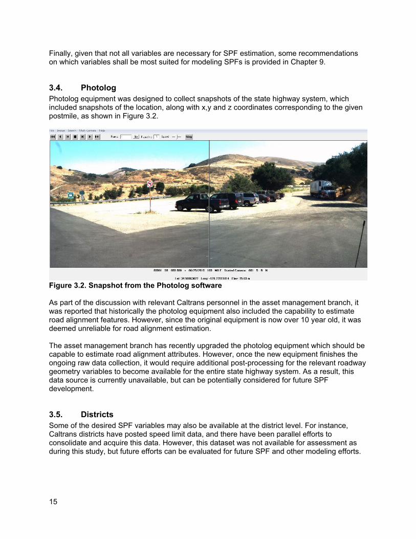
3.4. Photolog Photolog equipment was designed to collect snapshots of the state highway system, which included snapshots of the location, along with x,y and z coordinates corresponding to the given postmile, as shown in Figure 3.2.
Figure 3.2. Snapshot from the Photolog software
As part of the discussion with relevant Caltrans personnel in the asset management branch, it was reported that historically the photolog equipment also included the capability to estimate road alignment features. However, since the original equipment is now over 10 year old, it was deemed unreliable for road alignment estimation.
The asset management branch has recently upgraded the photolog equipment which should be capable to estimate road alignment attributes. However, once the new equipment finishes the ongoing raw data collection, it would require additional post-processing for the relevant roadway geometry variables to become available for the entire state highway system. As a result, this data source is currently unavailable, but can be potentially considered for future SPF development.
3.5. Districts Some of the desired SPF variables may also be available at the district level. For instance, Caltrans districts have posted speed limit data, and there have been parallel efforts to consolidate and acquire this data. However, this dataset was not available for assessment as during this study, but future efforts can be evaluated for future SPF and other modeling efforts.
15
4. SUITABILITY ANALYSIS OF EXISTING DATA SOURCES WITHIN CALTRANS
While Chapter 3 provides an overview of different data sources in Caltrans and the variables that they may include, Chapter 4 focuses on conducting a detailed suitability analysis of those sources to ascertain whether they can be utilized for obtaining variables for SPF modeling.
4.1. Methodological framework To assess the suitability of a dataset, it is important to define a set of performance measures that can help evaluate the quality of the data. For example, the primary requirement for a data source should be that it is available for the entire state highway system. However, a complete data set may not be a sufficient condition for a data source, as it should also have enough resolution over time and space so that it can be used for extracting meaningful variables for SPF modeling. Thus, three performance metrics have been proposed as part of this project to provide a comprehensive understanding of a given data element.
4.1.1. Proposed metrics CompletenessThe completeness of a data element is defined by whether a variable is populated across the entire state highway system for the relevant attribute (segments, intersections and ramps). It is the most fundamental attribute for a data element because an incompletely populated data element impacts the selection of the derived explanatory variable for SPF modeling. The completeness of a variable will be defined by % of observations that is available across the state highway system.
Frequency of updatesFrequency of updates for a data element is defined by how often a variable changes over time. Lack of updates for a data element implies that a variable may be outdated, thus resulting in a bias during SPF estimation/prediction. The intent of calculating frequency of updates is to identify variables that display significant temporal trend during data collection period. Therefore, for each spatial unit of observation for a data element, the number of historical changes made during a data collection period can be analyzed. The primary measure that can be calculated from these historical changes is years per update (yrs_per_update), which is defined as the years of data collection period divided by the number of changes. A secondary measure that can also be computed is the years since last update, to differentiate between the latest trends in the updates and the overall trend in the dataset.
Spatial variationSpatial variation is defined as how frequently a variable’s value changes across a highway route. Spatial variation, or more importantly, lack thereof, impacts the utility of a data element in two ways. First, lack of variation in the data across the network can impact the statistical significance of the variable in SPF modeling. Second, lack of variation in some instances may also be symptomatic of measurement biases when there are changes in the physical environment. For example, if annual daily traffic does not change even though number of lanes does, there may be an error in either of the two variables. The primary measures used for spatial variation are: (1) the amount of change in value of two consecutive spatial observations of a numeric variable; and (2) average number of miles per change, i.e., accumulated postmiles divided by number of changes, for both numeric and character variables.
16
4.1.2. Outlier analysis As Figure 4.1 suggests, a data element can potentially have a lot of variation in the quality of observations available across the state highway system. An important question is how to define suitability for the purposes of this study. Since it is essential to maximize the amount of data that can become available for SPF modeling, it is more appropriate to exclude poor quality data, as opposed to including only good quality data. Therefore, the project utilizes outlier analysis to identify thresholds for determining poor quality data.
Figure 4.1. Abstract representation of a data quality spectrum
Specifically, the study employs two types of statistical methods to flag outliers: (i) using 99% confidence intervals using assumptions of normal distribution, and (ii) interquartile ranges.
4.2. Analysis of data sources within Caltrans
4.2.1. TASAS
4.2.1.1. Segments The sections below first provides an overview of the state highway network (as developed using the TASAS data provided to the project team), followed by an assessment of the elements across three performance measures: completeness, frequency of updates, and spatial variation. Collectively, these performance measures inform the team of (i) whether a variable of interest is populated across the state highway system (completeness), (ii) how often it changes over time within the database (frequency of updates), (iii) how the value of a variable changes as it is observed across a route (spatial variation)
An R-based (R Core Team, 2016) mapping tool was developed to visualize and analyze the TASAS data structure. In addition to the TASAS highway segment data, Caltrans GIS data from the State Highway Network (SHN) and Postmile System (http://www.dot.ca.gov/hq/tsip/gis/datalibrary/)were utilized to construct the roadway and postmile layers. The State Highway Network (SHN) and Postmile GIS database contain information on highway line and postmile feature layers. Each record in the line layer represents a highway segment with longitude/latitude coordinates where the county, route, beginning postmile, ending postmile, postmile prefix, and postmile suffix are the same. The postmile layer contains valid postmile points at 0.1 (1/10th) mile intervals. Each record in the postmile layer represents one point with longitude/latitude coordinates and other features such as county, route, district, and PM.
It should be noted that the Caltrans GIS data from the State Highway Network and Postmile System is also used in the calculation of radius of curvature (horizontal alignment) and elevation (vertical alignment).
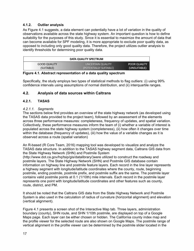
Figure 4.1 presents a screen shot of the Interactive Map tab. Three layers, administration boundary (county), SHN route, and SHN 1/10th postmile, are displayed on top of a Google Maps page. Each layer can be either chosen or hidden. The California county index map and the profile viewer for the selected route are also shown on Google Maps. The postmile range of vertical alignment in the profile viewer can be determined by the postmile slider located in the
17
left panel. In the left panel, query items regarding administration, county, route, functional class, and postmile range of vertical alignment are available for inspecting specific route or providing statistic summary.
Figure 4.1. Screen shot of “Interactive Map” tab of the R-based mapping tool
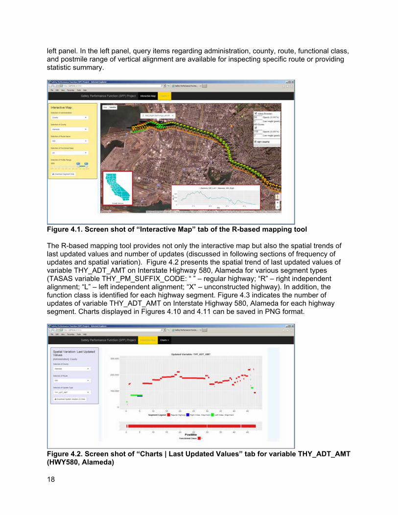
The R-based mapping tool provides not only the interactive map but also the spatial trends of last updated values and number of updates (discussed in following sections of frequency of updates and spatial variation). Figure 4.2 presents the spatial trend of last updated values of variable THY_ADT_AMT on Interstate Highway 580, Alameda for various segment types (TASAS variable THY_PM_SUFFIX_CODE: “ ” – regular highway; “R” – right independent alignment; “L” – left independent alignment; “X” – unconstructed highway). In addition, the function class is identified for each highway segment. Figure 4.3 indicates the number of updates of variable THY_ADT_AMT on Interstate Highway 580, Alameda for each highway segment. Charts displayed in Figures 4.10 and 4.11 can be saved in PNG format.
Figure 4.2. Screen shot of “Charts | Last Updated Values” tab for variable THY_ADT_AMT (HWY580, Alameda)
18

Figure 4.3. Screen shot of “Charts | Number of Updates” tab for variable THY_ADT_AMT (HWY580, Alameda)
[Note: It should be noted that the mapping tool is still under development at the time of preparing this document.]
Verification of Network CompletenessBy inspecting TASAS data using the mapping tool, gaps were found between highway segments,motivating study of the network completeness. As an example shows in Figure 4.3, several observations arefound for State Highway 84, Alameda as follows:
• The last updated values of variable THY_ADT_AMT jump up and down with various functional classes.
• Three gaps were identified, which raises the question of whether the missing postmiles were generated due to input error or initially not covered by state agency.
• By looking carefully at PM28, an overlap segment with two different recorded AADTs is perceived.
Figure 4.3. Last updated values of AADT across different functional classes of HWY84, Alameda
19

In the verification of network completeness, two assumptions were made: (1) the postmile of each individual route starts at zero; and (2) the cumulated post mileages of overlapped segment were excluded in the calculation of network completeness. The measure of network completeness is the percent completeness (PC) which is defined as the percentage of available postmiles [APM; excluded overlapped postmiles (OPM)] divided by sum of APM and gapped postmiles (GPM).
Figure 4.4 compares the values of percentage completeness by Caltrans district, which range from 81% (District 3) to 96% (District 11). Almost eight out of twelve districts have percentages of completeness greater than 90%.
Figure 4.4. Summary of network completeness by Caltrans district
Frequency of Updates
Definition and Methodology Figure 4.15 illustrates the methodology used to transform raw segment file into the file containing information of frequency of updates, which is designated as the frequency update file for following discussion. In Figure 4.5, segment identification variables for the analysis of frequency of updates include COUNTY, THY_FUNCTIONAL_CLASS_CODE, THY_PM_SUFFIX_CODE, THY_ROUTE_NAME, THY_BEGIN_PM_AMT, THY_END_PM_AMT, THY_ELEMENT_ID, and THY_LANDMARK_SHORT_DESC.
20

Figure 4.5. Methodology to transform raw TASAS highway segment file into a file containing essential information of frequency of updates
Dates in this analysis mainly consist of THY_BEGIN_DATE and THY_END_DATE. The date 01-01-3000 in the raw TASAS segment file was remarked as 04-21-2016 (the date when SafeTREC received TASAS data from Caltrans). Notice that the gradual color change in Figure 4.5 stands for the changes of cell values whereas constant cell values are in the same color. The outputs mainly include beginning and ending dates of data collection period (date_period_beg and date_period_end), last updated value (last_update_value), number of changes (no_of_change), and years per update (yrs_per_update). Figure 4.6 illustrates the definitions of last_update_date, last_update_value (pointed by red arrow), and no_of_change at various AADT cases. As shown in Figure 4.6, the last_update_date is exactly the same as the date_period_end.
Figure 4.6. Definitions of last_update_date and number of change using AADT as an exampleIn this segment analysis, the variables considered are as follows:
Numeric variables: THY_ADT_AMT THY_DESIGN_SPEED_AMT THY_LT_LANES_AMT THY_LT_O_SHD_TOT_WIDTH_AMT THY_LT_O_SHD_TRT_WIDTH_AMT THY_LT_TRAV_WAY_WIDTH_AMT THY_MEDIAN_WIDTH_AMT THY_RT_LANES_AMT
21
THY_RT_O_SHD_TOT_WIDTH_AMT THY_RT_O_SHD_TRT_WIDTH_AMT THY_RT_TRAV_WAY_WIDTH_AMT
Character variables: THY_LT_SPEC_FEATURES_CODE THY_MEDIAN_BARRIER_CODE THY_MEDIAN_SIG_CHG_IND THY_MEDIAN_TYPE_CODE THY_MEDIAN_WIDTH_VAR_CODE THY_RT_SPEC_FEATURES_CODE
Variables are categorize into numeric and character variables so that character variables can be used to calculate the measures of yrs_per_update or miles_per_change (discussed in spatial variation section), but not in calculating ∆y distribution (difference of last_update_value values in two consecutive segments; discussed in the spatial variation section).
Results and Discussions
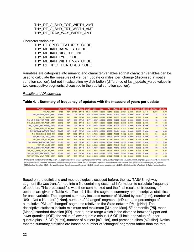
Table 4.1. Summary of frequency of updates with the measure of years per update
Based on the definitions and methodologies discussed before, the raw TASAS highway segment file was transformed into a file containing essential information to calculate frequency of updates. This processed file was then summarized and the final results of frequency of updates are given in Table 4.1. Table 4.1 lists the segment summary and descriptive statistics for each variable. The segment summary includes number of “divided by zero” [nInf], number of “0/0 – Not a Number” [nNan], number of “changed” segments [nData], and percentage of cumulative PMs of “changed” segments relative to the State network PMs [pNet]. The descriptive statistics include minimum and maximum [Min and Max], 5th percentile [P5], mean [Mean], standard deviation [SD], inter-quartile range which is the distance between upper and lower quartiles [IQR], the value of lower quartile minus 1.5IQR [lLimit], the value of upper quartile plus 1.5IQR [rLimit], number of outliers [nOutlier], and percent outliers [pOutlier]. Notice that the summary statistics are based on number of “changed” segments rather than the total
22

segments. In the segment summary, two cases are worth mentioning as follows: (1) “divided by zero” segments – segments without changes/updates (no_of_change = 0); and (2) “0/0 – Not a Number” segments – segments satisfied with the criteria: date_period_beg = date_period_end&no_of_change = 0.
It should be noted that, in Table 4.1, the variables other than THY_ADT_AMT have zero IQR values; that is to say, those variables have the same values of lower and upper quartiles and it implies that only a few number of unique values of yrs_per_update for those variables are found and it indicates that those variables were not updated very frequently.As shown in Table 4.1, the AADT variable (THY_ADT_AMT) has the smallest mean value (3.3202) of yrs_per_update, with a segment update percentage (PNET) as high as 87% of the entire California network. Conversely, all the other considered variables show a segment update percentage close to or less than one percent.
Figure 4.7 illustrates the choropleth map and summary table of mean values of yrs_per_update of AADT variable by county. The summary table in Figure 4.17 was ranked by mean value (highlighted in red). The smallest mean value of yrs_per_update (1.88) was found in Santa Barbara County,while the largest mean value of yrs_per_update (7.62) was found in Sierra County.
Figure 4.8compares the mean values of yrs_per_update of AADT variable by Caltrans district. As shown, District 8 has the largest mean value of yrs_per_update (4.9) compared with the smallest mean value of yrs_per_update (2.1) for District 7. Notice that the larger the mean value, the slower the update.
Figure 4.7. Mean values of yrs_per_update of AADT variable by county
23
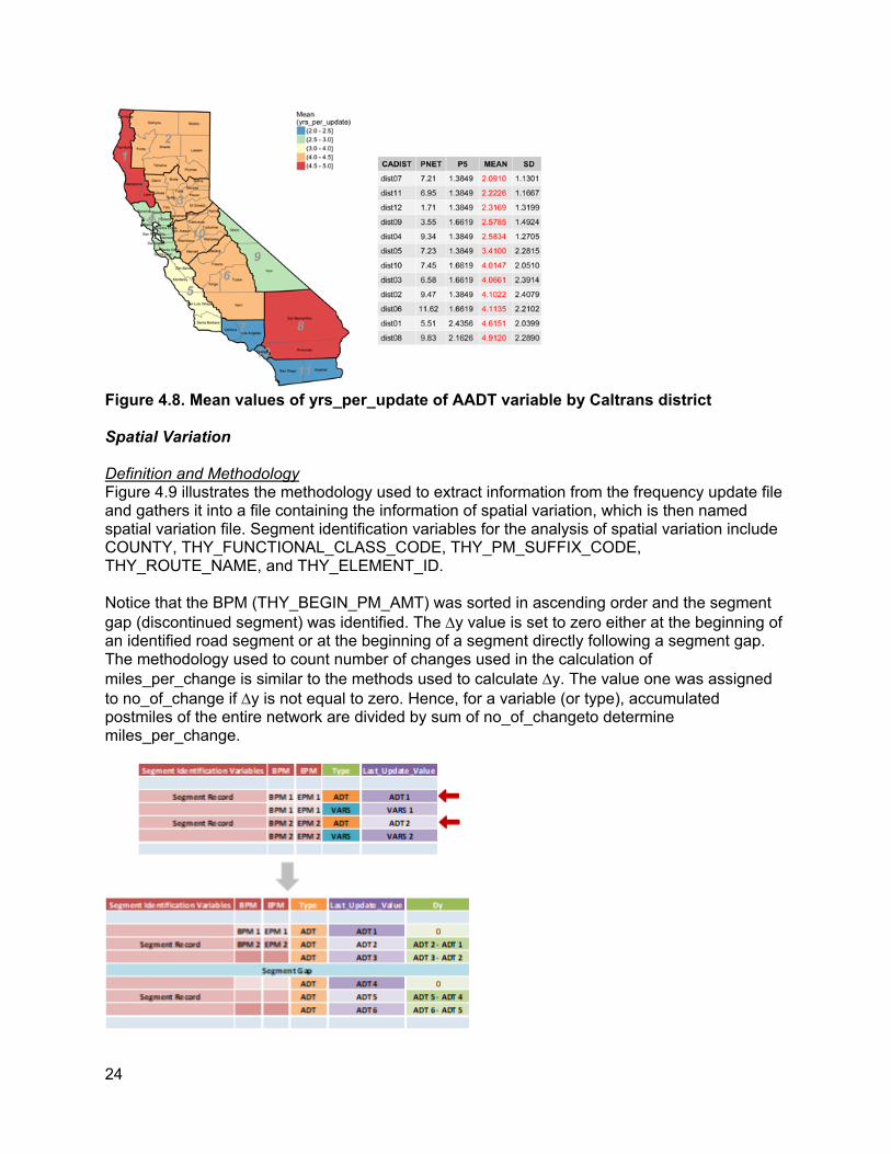
Figure 4.8. Mean values of yrs_per_update of AADT variable by Caltrans district
Spatial Variation
Definition and Methodology Figure 4.9 illustrates the methodology used to extract information from the frequency update file and gathers it into a file containing the information of spatial variation, which is then named spatial variation file. Segment identification variables for the analysis of spatial variation include COUNTY, THY_FUNCTIONAL_CLASS_CODE, THY_PM_SUFFIX_CODE, THY_ROUTE_NAME, and THY_ELEMENT_ID.
Notice that the BPM (THY_BEGIN_PM_AMT) was sorted in ascending order and the segment gap (discontinued segment) was identified. The ∆y value is set to zero either at the beginning of an identified road segment or at the beginning of a segment directly following a segment gap. The methodology used to count number of changes used in the calculation of miles_per_change is similar to the methods used to calculate ∆y. The value one was assigned to no_of_change if ∆y is not equal to zero. Hence, for a variable (or type), accumulated postmiles of the entire network are divided by sum of no_of_changeto determine miles_per_change.
24
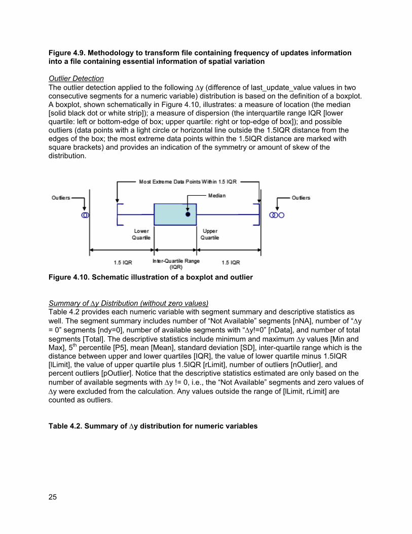
Figure 4.9. Methodology to transform file containing frequency of updates information into a file containing essential information of spatial variation
Outlier Detection The outlier detection applied to the following ∆y (difference of last_update_value values in two consecutive segments for a numeric variable) distribution is based on the definition of a boxplot. A boxplot, shown schematically in Figure 4.10, illustrates: a measure of location (the median [solid black dot or white strip]); a measure of dispersion (the interquartile range IQR [lower quartile: left or bottom-edge of box; upper quartile: right or top-edge of box]); and possible outliers (data points with a light circle or horizontal line outside the 1.5IQR distance from the edges of the box; the most extreme data points within the 1.5IQR distance are marked with square brackets) and provides an indication of the symmetry or amount of skew of the distribution.
Figure 4.10. Schematic illustration of a boxplot and outlier
Summary of ∆y Distribution (without zero values) Table 4.2 provides each numeric variable with segment summary and descriptive statistics as well. The segment summary includes number of “Not Available” segments [nNA], number of “∆y = 0” segments [ndy=0], number of available segments with “∆y!=0” [nData], and number of total segments [Total]. The descriptive statistics include minimum and maximum ∆y values [Min and Max], 5th percentile [P5], mean [Mean], standard deviation [SD], inter-quartile range which is the distance between upper and lower quartiles [IQR], the value of lower quartile minus 1.5IQR [lLimit], the value of upper quartile plus 1.5IQR [rLimit], number of outliers [nOutlier], and percent outliers [pOutlier]. Notice that the descriptive statistics estimated are only based on the number of available segments with ∆y != 0, i.e., the “Not Available” segments and zero values of ∆y were excluded from the calculation. Any values outside the range of [lLimit, rLimit] are counted as outliers.
Table 4.2. Summary of ∆y distribution for numeric variables
25
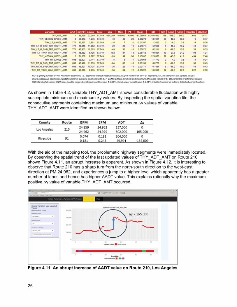
As shown in Table 4.2, variable THY_ADT_AMT shows considerable fluctuation with highly susceptible minimum and maximum ∆y values. By inspecting the spatial variation file, the consecutive segments containing maximum and minimum ∆y values of variable THY_ADT_AMT were identified as shown below:
With the aid of the mapping tool, the problematic highway segments were immediately located. By observing the spatial trend of the last updated values of THY_ADT_AMT on Route 210 shown Figure 4.11, an abrupt increase is apparent. As shown in Figure 4.12, it is interesting to observe that Route 210 has a sharp turn from the north-south direction to the west-east direction at PM 24.962, and experiences a jump to a higher level which apparently has a greater number of lanes and hence has higher AADT value. This explains rationally why the maximum positive ∆y value of variable THY_ADT_AMT occurred.
Figure 4.11. An abrupt increase of AADT value on Route 210, Los Angeles
26
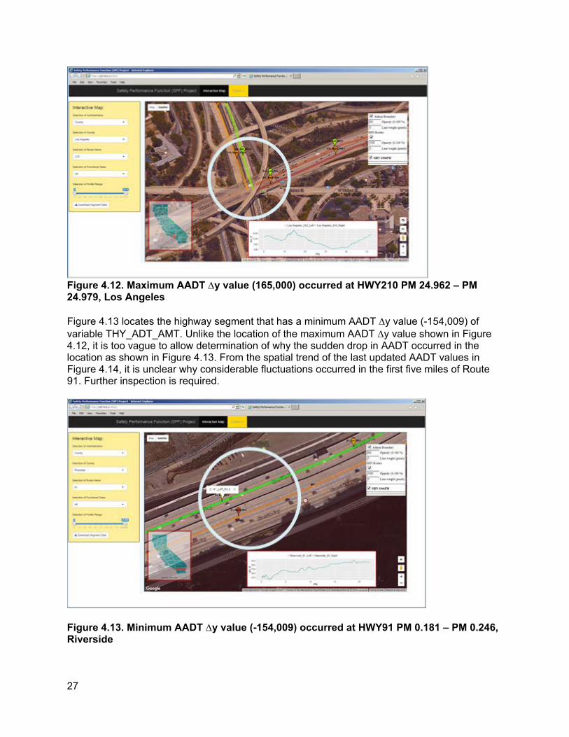
Figure 4.12. Maximum AADT ∆y value (165,000) occurred at HWY210 PM 24.962 – PM 24.979, Los Angeles
Figure 4.13 locates the highway segment that has a minimum AADT ∆y value (-154,009) of variable THY_ADT_AMT. Unlike the location of the maximum AADT ∆y value shown in Figure 4.12, it is too vague to allow determination of why the sudden drop in AADT occurred in the location as shown in Figure 4.13. From the spatial trend of the last updated AADT values in Figure 4.14, it is unclear why considerable fluctuations occurred in the first five miles of Route 91. Further inspection is required.
Figure 4.13. Minimum AADT ∆y value (-154,009) occurred at HWY91 PM 0.181 – PM 0.246, Riverside
27
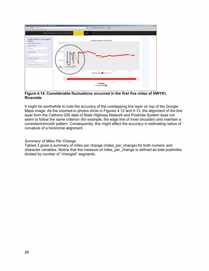
Figure 4.14. Considerable fluctuations occurred in the first five miles of HWY91, Riverside
It might be worthwhile to note the accuracy of the overlapping line layer on top of the Google Maps image. As the zoomed-in photos show in Figures 4.12 and 4.13, the alignment of the line layer form the Caltrans GIS date of State Highway Network and Postmile System does not seem to follow the same criterion (for example, the edge line of inner shoulder) and maintain a consistent/smooth pattern. Consequently, this might affect the accuracy in estimating radius of curvature of a horizontal alignment.
Summary of Miles Per Change Table4.3 gives a summary of miles per change (miles_per_change) for both numeric and character variables. Notice that the measure of miles_per_change is defined as total postmiles divided by number of “changed” segments.
28
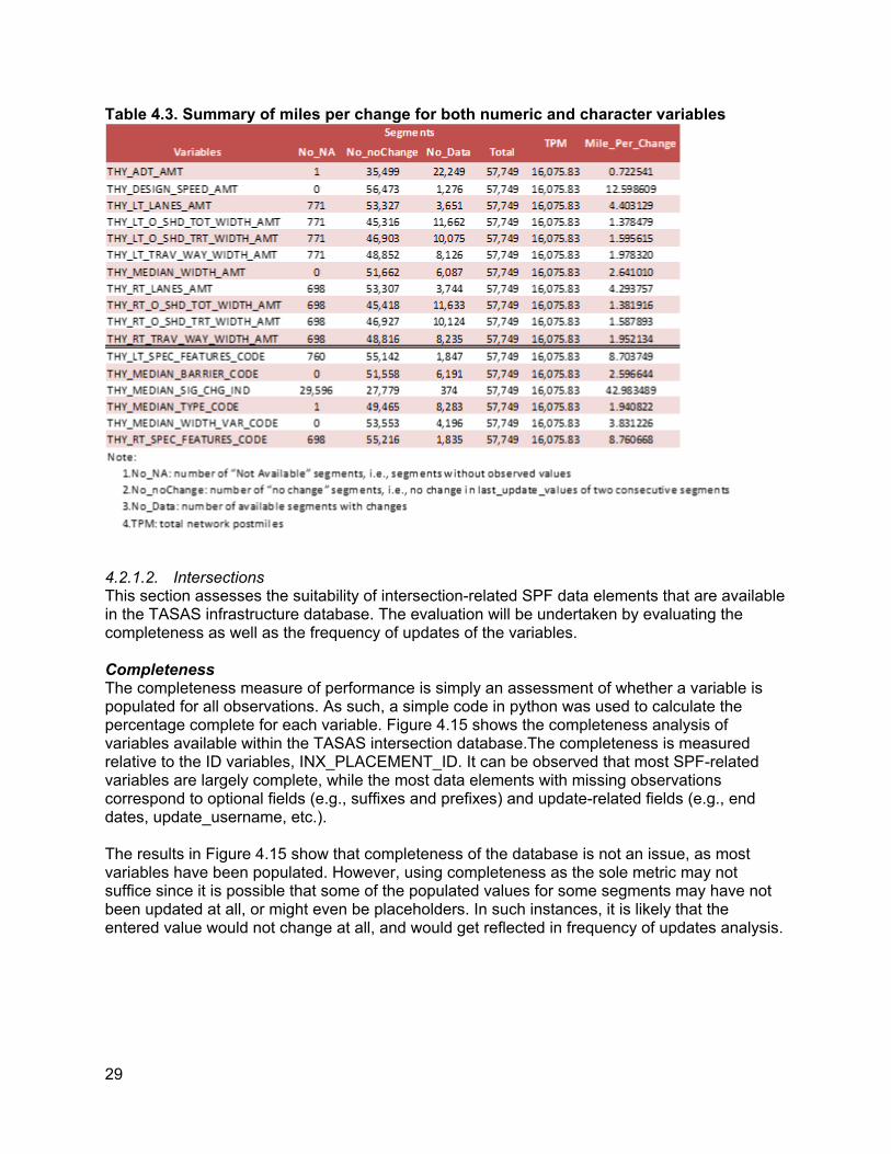
Table 4.3. Summary of miles per change for both numeric and character variables
4.2.1.2. Intersections This section assesses the suitability of intersection-related SPF data elements that are available in the TASAS infrastructure database. The evaluation will be undertaken by evaluating the completeness as well as the frequency of updates of the variables.
CompletenessThe completeness measure of performance is simply an assessment of whether a variable is populated for all observations. As such, a simple code in python was used to calculate the percentage complete for each variable. Figure 4.15 shows the completeness analysis of variables available within the TASAS intersection database.The completeness is measured relative to the ID variables, INX_PLACEMENT_ID. It can be observed that most SPF-related variables are largely complete, while the most data elements with missing observations correspond to optional fields (e.g., suffixes and prefixes) and update-related fields (e.g., end dates, update_username, etc.).
The results in Figure 4.15 show that completeness of the database is not an issue, as most variables have been populated. However, using completeness as the sole metric may not suffice since it is possible that some of the populated values for some segments may have not been updated at all, or might even be placeholders. In such instances, it is likely that the entered value would not change at all, and would get reflected in frequency of updates analysis.
29
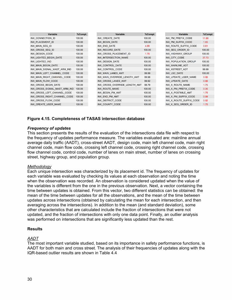
Figure 4.15. Completeness of TASAS intersection database
Frequency of updatesThis section presents the results of the evaluation of the intersections data file with respect to the frequency of updates performance measure. The variables evaluated are: mainline annual average daily traffic (AADT), cross-street AADT, design code, main left channel code, main right channel code, main flow code, crossing left channel code, crossing right channel code, crossing flow channel code, control code, number of lanes on main street, number of lanes on crossing street, highway group, and population group.
Methodology Each unique intersection was characterized by its placement id. The frequency of updates for each variable was evaluated by checking its values at each observation and noting the time when the observation was recorded. An observation is considered updated when the value of the variables is different from the one in the previous observation. Next, a vector containing the time between updates is obtained. From this vector, two different statistics can be obtained: the mean of the time between updates for all the observations, and the mean of the time between updates across intersections (obtained by calculating the mean for each intersection, and then averaging across the intersections). In addition to the mean (and standard deviation), some other characteristics that are calculated include the fraction of intersections that were not updated, and the fraction of intersections with only one data point. Finally, an outlier analysis was performed on intersections that are significantly less updated than the rest.
Results
AADT The most important variable studied, based on its importance in safety performance functions, is AADT for both main and cross street. The analysis of their frequencies of updates along with the IQR-based outlier results are shown in Table 4.4
30
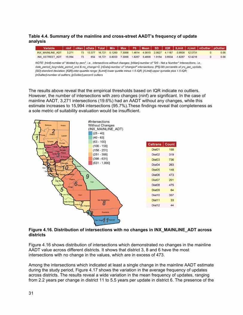
Table 4.4. Summary of the mainline and cross-street AADT’s frequency of update analysis
The results above reveal that the empirical thresholds based on IQR indicate no outliers. However, the number of intersections with zero changes (ninf) are significant. In the case of mainline AADT, 3,271 intersections (19.6%) had an AADT without any changes, while this estimate increases to 15,994 intersections (95.7%).These findings reveal that completeness as a sole metric of suitability evaluation would be insufficient.
Figure 4.16. Distribution of intersections with no changes in INX_MAINLINE_ADT across districts
Figure 4.16 shows distribution of intersections which demonstrated no changes in the mainline AADT value across different districts. It shows that district 3, 8 and 6 have the most intersections with no change in the values, which are in excess of 473.
Among the intersections which indicated at least a single change in the mainline AADT estimate during the study period, Figure 4.17 shows the variation in the average frequency of updates across districts. The results reveal a wide variation in the mean frequency of updates, ranging from 2.2 years per change in district 11 to 5.5 years per update in district 6. The presence of the
31
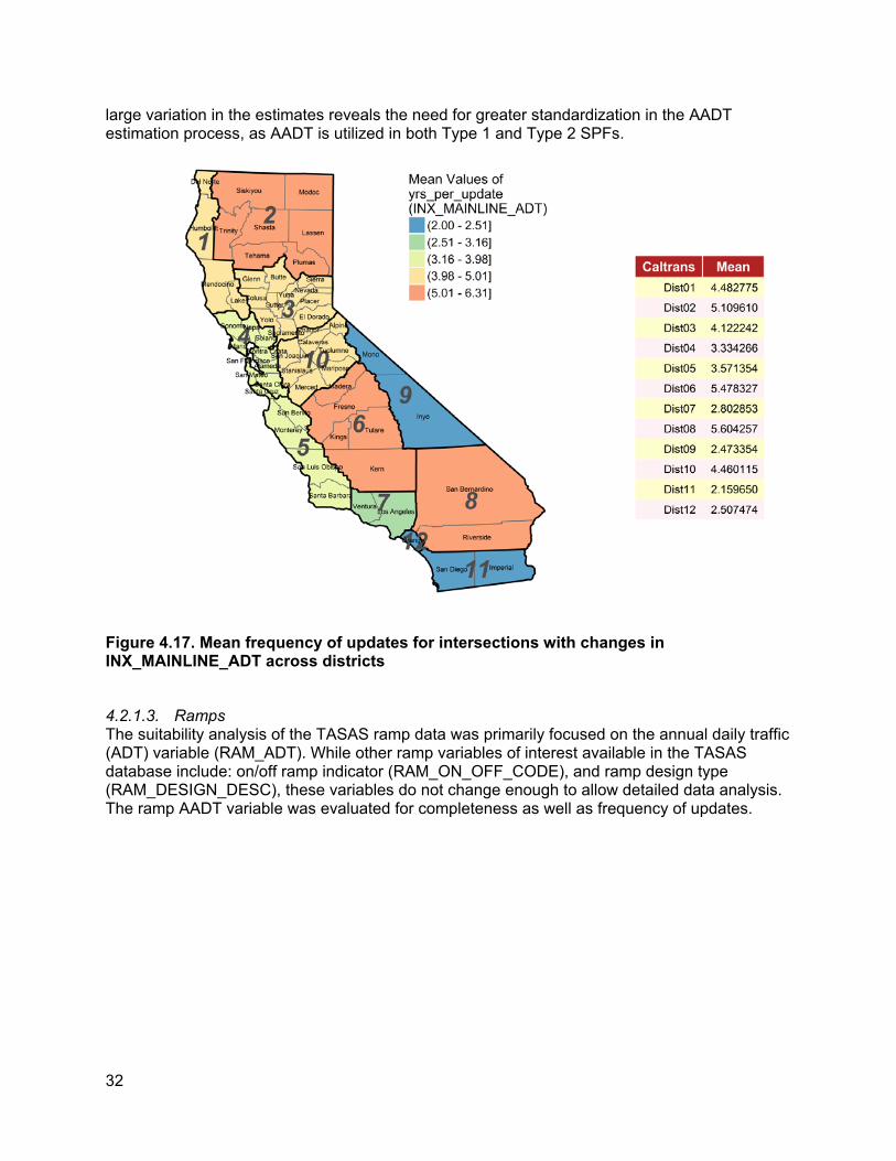
large variation in the estimates reveals the need for greater standardization in the AADT estimation process, as AADT is utilized in both Type 1 and Type 2 SPFs.
Figure 4.17. Mean frequency of updates for intersections with changes in INX_MAINLINE_ADT across districts
4.2.1.3. Ramps The suitability analysis of the TASAS ramp data was primarily focused on the annual daily traffic (ADT) variable (RAM_ADT). While other ramp variables of interest available in the TASAS database include: on/off ramp indicator (RAM_ON_OFF_CODE), and ramp design type (RAM_DESIGN_DESC), these variables do not change enough to allow detailed data analysis. The ramp AADT variable was evaluated for completeness as well as frequency of updates.
32
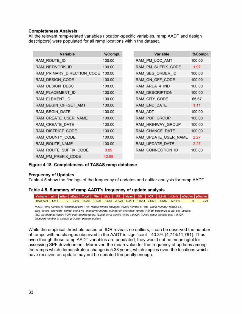
Completeness AnalysisAll the relevant ramp-related variables (location-specific variables, ramp AADT and design descriptors) were populated for all ramp locations within the dataset.
Figure 4.18. Completeness of TASAS ramp database
Frequency of UpdatesTable 4.5 show the findings of the frequency of updates and outlier analysis for ramp AADT.
Table 4.5. Summary of ramp AADT’s frequency of update analysis
While the empirical threshold based on IQR reveals no outliers, it can be observed the number of ramps with no changes observed in the AADT is significant—40.3% (4,744/11,761). Thus, even though these ramp AADT variables are populated, they would not be meaningful for assessing SPF development. Moreover, the mean value for the frequency of updates among the ramps which demonstrate a change is 5.38 years, which implies even the locations which have received an update may not be updated frequently enough.
33

Figure 4.19. Distribution of ramps with no changes in RAM_ADT across districts
To further evaluate the variation across districts, Figure 4.19 indicates that the districts with most ramps without AADT changes are district 7 and 4, with over 1,150 ramps not showing any variation in the ramp AADT values during the period being investigated (2008-2016).
Among the ramps for which RAM_ADT showed at least a single variable change, the mean frequency changes from 3 years/update to 6.7 years/update. In the case of districts 8 and 9, none of the ramps displayed any change in its value. Thus, similar to the findings observed in mainline AADT, there is a need for greater standardization of AADT updates for ramps.
34
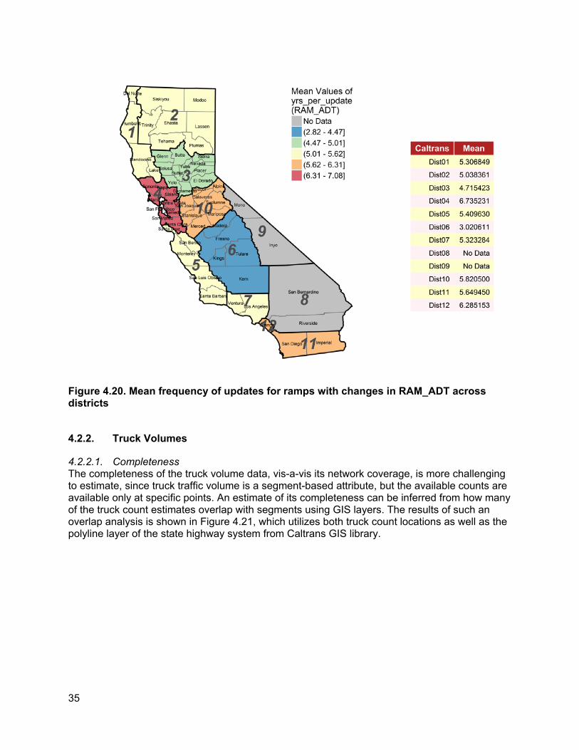
Figure 4.20. Mean frequency of updates for ramps with changes in RAM_ADT across districts
4.2.2. Truck Volumes
4.2.2.1. Completeness The completeness of the truck volume data, vis-a-vis its network coverage, is more challenging to estimate, since truck traffic volume is a segment-based attribute, but the available counts are available only at specific points. An estimate of its completeness can be inferred from how many of the truck count estimates overlap with segments using GIS layers. The results of such an overlap analysis is shown in Figure 4.21, which utilizes both truck count locations as well as the polyline layer of the state highway system from Caltrans GIS library.
35

Figure 4.21. Visual representation of truck counts over the network
Based on the results of the overlap analysis, it can be estimated that 19.23% of the highway network (by post miles) do not have an overlapping count location. Thus, the available truck volume counts cannot be estimated using this data source for the entire state highway system.
In addition, as Table 4.6 indicates, among the observations that were available, there have been instances of not all variables being completely populated across reporting years.
Table 4.6. Variable-specific Completeness within the database Year of Data Provided
Vehicle AADT Total
Truck AADT Total
Axle 2 Axle 3 Axle 4 Axle 5+ EAL 2-Way (1000)
Year Verified/ Updated
2010 100% 100% 100% 100% 100% 100% 0% 99.97%
2011 100% 100% 100% 100% 100% 100% 100% 100%
2012 99.94% 99.94% 99.94% 99.94% 99.94% 99.94% 100% 100%
2013 100% 100% 100% 100% 100% 100% 100% 100%
2014 100% 100% 100% 100% 100% 100% 100% 100%
4.2.2.2. Time since last update While the years of data provided for the truck count locations are recent and periodic, the more relevant variable to consider regarding updates is the year the count was last verified/updated. Table 4.7 shows the results of an outlier analysis conducted using the last year of count verification/update.
36
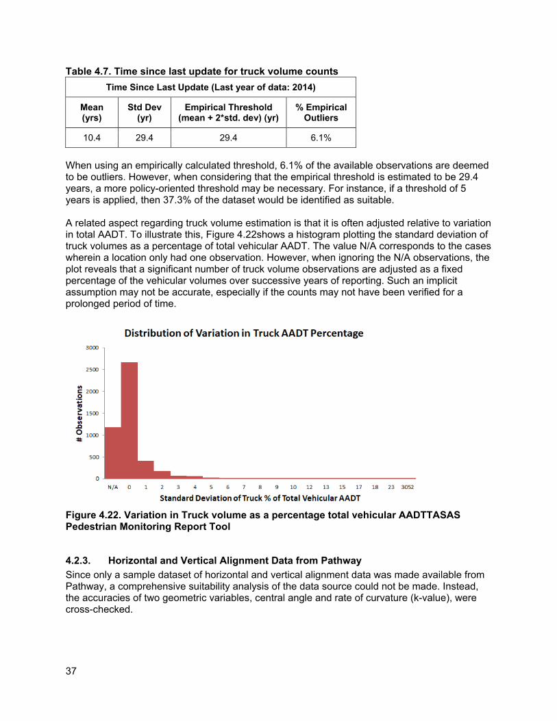
Table 4.7. Time since last update for truck volume counts Time Since Last Update (Last year of data: 2014)
Mean (yrs)
Std Dev (yr)
Empirical Threshold (mean + 2*std. dev) (yr)
% EmpiricalOutliers
10.4 29.4 29.4 6.1%
When using an empirically calculated threshold, 6.1% of the available observations are deemed to be outliers. However, when considering that the empirical threshold is estimated to be 29.4 years, a more policy-oriented threshold may be necessary. For instance, if a threshold of 5 years is applied, then 37.3% of the dataset would be identified as suitable.
A related aspect regarding truck volume estimation is that it is often adjusted relative to variation in total AADT. To illustrate this, Figure 4.22shows a histogram plotting the standard deviation of truck volumes as a percentage of total vehicular AADT. The value N/A corresponds to the cases wherein a location only had one observation. However, when ignoring the N/A observations, the plot reveals that a significant number of truck volume observations are adjusted as a fixed percentage of the vehicular volumes over successive years of reporting. Such an implicit assumption may not be accurate, especially if the counts may not have been verified for a prolonged period of time.
Figure 4.22. Variation in Truck volume as a percentage total vehicular AADTTASAS Pedestrian Monitoring Report Tool
4.2.3. Horizontal and Vertical Alignment Data from Pathway Since only a sample dataset of horizontal and vertical alignment data was made available from Pathway, a comprehensive suitability analysis of the data source could not be made. Instead, the accuracies of two geometric variables, central angle and rate of curvature (k-value), were cross-checked.
37
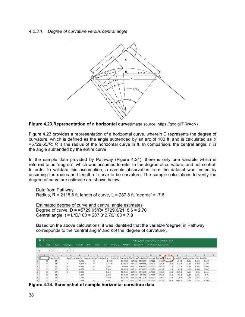
4.2.3.1. Degree of curvature versus central angle
Figure 4.23.Representation of a horizontal curve(Image source: https://goo.gl/PRrAdN)
Figure 4.23 provides a representation of a horizontal curve, wherein D represents the degree of curvature, which is defined as the angle subtended by an arc of 100 ft, and is calculated as 𝐷𝐷 =5729.65/R; R is the radius of the horizontal curve in ft. In comparison, the central angle, t, is the angle subtended by the entire curve.
In the sample data provided by Pathway (Figure 4.24), there is only one variable which is referred to as “degree”, which was assumed to refer to the degree of curvature, and not central. In order to validate this assumption, a sample observation from the dataset was tested by assuming the radius and length of curve to be curvature. The sample calculations to verify the degree of curvature estimate are shown below:
Data from Pathway Radius, R = 2118.6 ft, length of curve, L = 287.8 ft, ‘degree’ = -7.8
Estimated degree of curve and central angle estimates Degree of curve, D = =5729.65/R= 5729.6/2118.6 = 2.70 Central angle, t = L*D/100 = 287.8*2.70/100 = 7.8
Based on the above calculations, it was identified that the variable ‘degree’ in Pathway corresponds to the ‘central angle’ and not the ‘degree of curvature’.
Figure 4.24. Screenshot of sample horizontal curvature data
38

4.2.3.2. Rate of curvature (K)
Figure 4.25 represents a typical vertical curve, wherein G1 and G2 arethe tangent grades in percentA is algebraic difference in grade, L is the length of vertical curve, and E is the vertical offset.
Figure 4.25. Representation of a vertical curve(Image source: https://goo.gl/r8ZRHW)
The rate of change of grade at successive points on the curve is a constant amount for equal increments of horizontal distance, and is equal to the algebraic difference between intersecting tangent grades divided by the length of curve in feet, or A/L. The reciprocal of this estimate, L/A, termed 'K', is the horizontal distance in feet required to make 1% change in gradient and is therefore, a measure of curvature. It is expressed as ft/percent.
i.e., K = L/A Where, L - Length of vertical curve
A - Absolute value of difference in grades
In comparison, the K-value defined in the sample Pathway data is shown to have units of feet/degree, as shown in Figure 4.36. In order to confirm that the k-value is consistent with the grade and length of vertical curve estimates, the following sample calculation are done:
Data from Pathway G1 = -1.023%, G2 = -1.761%, L = 658.1 ft, K (in ft/deg)=891.2
Estimated degree of curve and central angle estimates A = |G1- G2| = |-1.761- -1.023| = 0.738 K = 658.1/0.738 = 891.7ft/percent
Based on the above sample calculation, it can be confirmed that K-value provided by Pathway should have units of ‘ft/percent’ and not the ‘ft/deg’.
Figure 4.26. Screenshot of sample vertical curvature data
The calculations shown in sections 4.2.3.1 and 4.2.3.2 reveal that the different geometric variable estimates provided by Pathway are internally consistent, although they have been defined inaccurately in some cases.
39
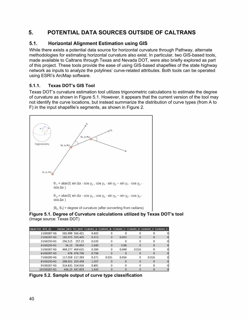
5. POTENTIAL DATA SOURCES OUTSIDE OF CALTRANS
5.1. Horizontal Alignment Estimation using GIS While there exists a potential data source for horizontal curvature through Pathway, alternate methodologies for estimating horizontal curvature also exist. In particular, two GIS-based tools, made available to Caltrans through Texas and Nevada DOT, were also briefly explored as part of this project. These tools provide the ease of using GIS-based shapefiles of the state highway network as inputs to analyze the polylines’ curve-related attributes. Both tools can be operated using ESRI’s ArcMap software.
5.1.1. Texas DOT’s GIS Tool Texas DOT’s curvature estimation tool utilizes trigonometric calculations to estimate the degree of curvature as shown in Figure 5.1. However, it appears that the current version of the tool may not identify the curve locations, but instead summarize the distribution of curve types (from A to F) in the input shapefile’s segments, as shown in Figure 2.
Figure 5.1. Degree of Curvature calculations utilized by Texas DOT’s tool (Image source: Texas DOT)
Figure 5.2. Sample output of curve type classification
40
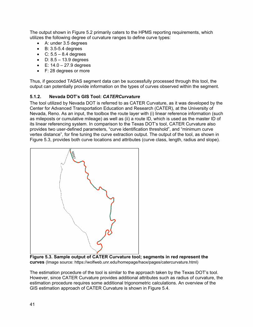
The output shown in Figure 5.2 primarily caters to the HPMS reporting requirements, which utilizes the following degree of curvature ranges to define curve types:
• A: under 3.5 degrees • B: 3.5-5.4 degrees • C: 5.5 – 8.4 degrees • D: 8.5 – 13.9 degrees • E: 14.0 – 27.9 degrees • F: 28 degrees or more
Thus, if geocoded TASAS segment data can be successfully processed through this tool, the output can potentially provide information on the types of curves observed within the segment.
5.1.2. Nevada DOT’s GIS Tool: CATERCurvature The tool utilized by Nevada DOT is referred to as CATER Curvature, as it was developed by the Center for Advanced Transportation Education and Research (CATER), at the University of Nevada, Reno. As an input, the toolbox the route layer with (i) linear reference information (such as mileposts or cumulative mileage) as well as (ii) a route ID, which is used as the master ID of its linear referencing system. In comparison to the Texas DOT’s tool, CATER Curvature also provides two user-defined parameters, “curve identification threshold”, and “minimum curve vertex distance”, for fine tuning the curve extraction output. The output of the tool, as shown in Figure 5.3, provides both curve locations and attributes (curve class, length, radius and slope).
Figure 5.3. Sample output of CATER Curvature tool; segments in red represent the curves (Image source: https://wolfweb.unr.edu/homepage/haox/pages/catercurvature.html)
The estimation procedure of the tool is similar to the approach taken by the Texas DOT’s tool. However, since CATER Curvature provides additional attributes such as radius of curvature, the estimation procedure requires some additional trigonometric calculations. An overview of the GIS estimation approach of CATER Curvature is shown in Figure 5.4.
41
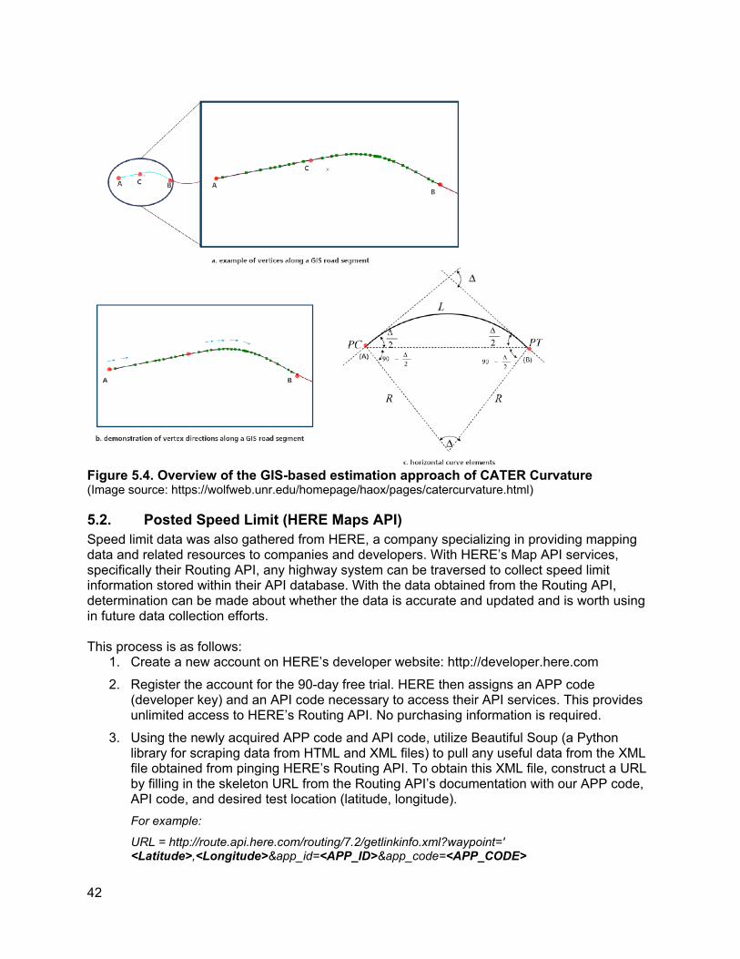
Figure 5.4. Overview of the GIS-based estimation approach of CATER Curvature (Image source: https://wolfweb.unr.edu/homepage/haox/pages/catercurvature.html)
5.2. Posted Speed Limit (HERE Maps API) Speed limit data was also gathered from HERE, a company specializing in providing mapping data and related resources to companies and developers. With HERE’s Map API services, specifically their Routing API, any highway system can be traversed to collect speed limit information stored within their API database. With the data obtained from the Routing API, determination can be made about whether the data is accurate and updated and is worth using in future data collection efforts.
This process is as follows: 1. Create a new account on HERE’s developer website: http://developer.here.com 2. Register the account for the 90-day free trial. HERE then assigns an APP code
(developer key) and an API code necessary to access their API services. This provides unlimited access to HERE’s Routing API. No purchasing information is required.
3. Using the newly acquired APP code and API code, utilize Beautiful Soup (a Python library for scraping data from HTML and XML files) to pull any useful data from the XML file obtained from pinging HERE’s Routing API. To obtain this XML file, construct a URL by filling in the skeleton URL from the Routing API’s documentation with our APP code, API code, and desired test location (latitude, longitude). For example:
URL = http://route.api.here.com/routing/7.2/getlinkinfo.xml?waypoint=' <Latitude>,<Longitude>&app_id=<APP_ID>&app_code=<APP_CODE>
42
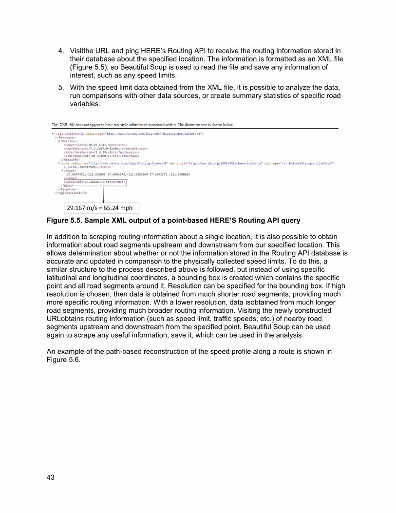
4. Visitthe URL and ping HERE’s Routing API to receive the routing information stored in their database about the specified location. The information is formatted as an XML file (Figure 5.5), so Beautiful Soup is used to read the file and save any information of interest, such as any speed limits.
5. With the speed limit data obtained from the XML file, it is possible to analyze the data, run comparisons with other data sources, or create summary statistics of specific road variables.
Figure 5.5. Sample XML output of a point-based HERE’S Routing API query
In addition to scraping routing information about a single location, it is also possible to obtain information about road segments upstream and downstream from our specified location. This allows determination about whether or not the information stored in the Routing API database is accurate and updated in comparison to the physically collected speed limits. To do this, a similar structure to the process described above is followed, but instead of using specific latitudinal and longitudinal coordinates, a bounding box is created which contains the specific point and all road segments around it. Resolution can be specified for the bounding box. If high resolution is chosen, then data is obtained from much shorter road segments, providing much more specific routing information. With a lower resolution, data isobtained from much longer road segments, providing much broader routing information. Visiting the newly constructed URLobtains routing information (such as speed limit, traffic speeds, etc.) of nearby road segments upstream and downstream from the specified point. Beautiful Soup can be used again to scrape any useful information, save it, which can be used in the analysis.
An example of the path-based reconstruction of the speed profile along a route is shown in Figure 5.6.
43
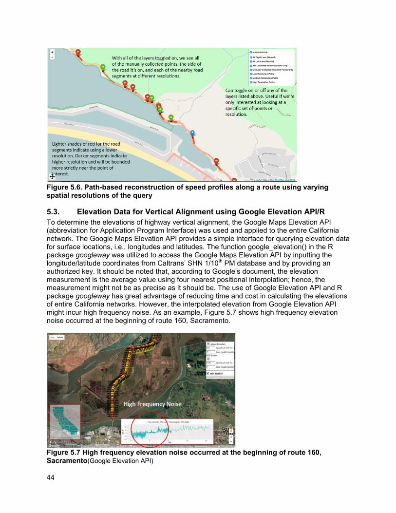
Figure 5.6. Path-based reconstruction of speed profiles along a route using varying spatial resolutions of the query
5.3. Elevation Data for Vertical Alignment using Google Elevation API/R To determine the elevations of highway vertical alignment, the Google Maps Elevation API (abbreviation for Application Program Interface) was used and applied to the entire California network. The Google Maps Elevation API provides a simple interface for querying elevation data for surface locations, i.e., longitudes and latitudes. The function google_elevation() in the R package googleway was utilized to access the Google Maps Elevation API by inputting the longitude/latitude coordinates from Caltrans’ SHN 1/10th PM database and by providing an authorized key. It should be noted that, according to Google’s document, the elevation measurement is the average value using four nearest positional interpolation; hence, the measurement might not be as precise as it should be. The use of Google Elevation API and R package googleway has great advantage of reducing time and cost in calculating the elevations of entire California networks. However, the interpolated elevation from Google Elevation API might incur high frequency noise. As an example, Figure 5.7 shows high frequency elevation noise occurred at the beginning of route 160, Sacramento.
Figure 5.7 High frequency elevation noise occurred at the beginning of route 160, Sacramento(Google Elevation API)
44
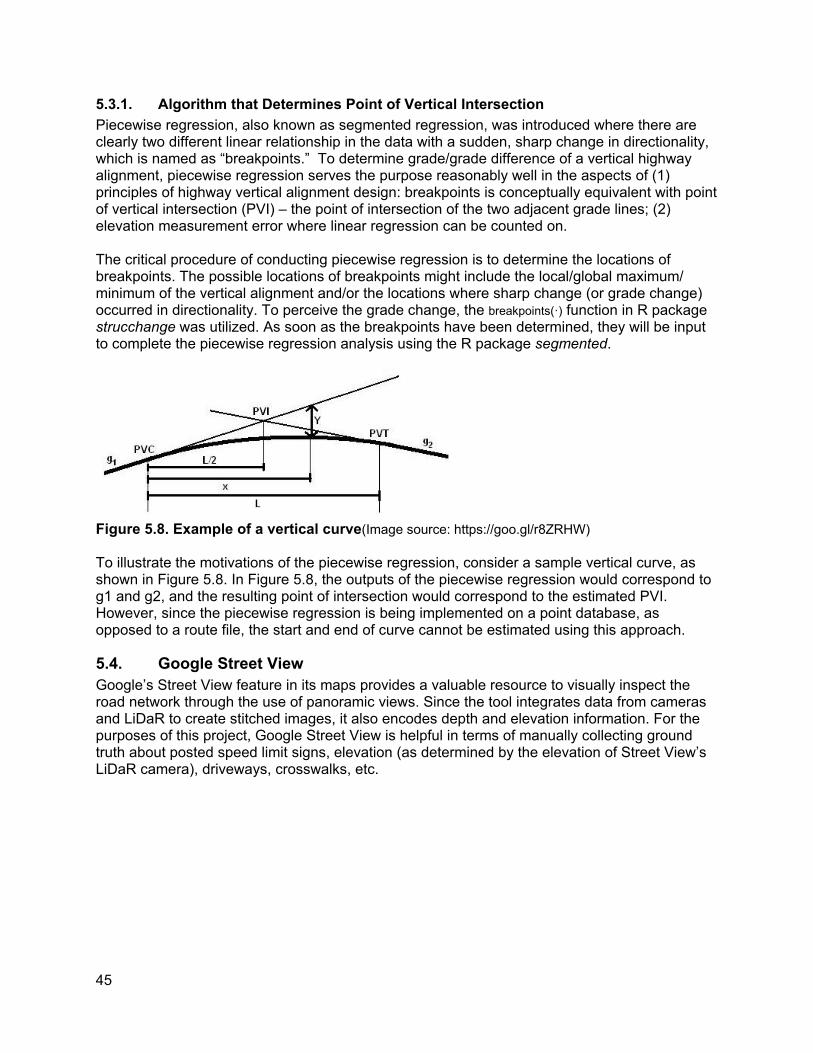
5.3.1. Algorithm that Determines Point of Vertical Intersection Piecewise regression, also known as segmented regression, was introduced where there are clearly two different linear relationship in the data with a sudden, sharp change in directionality, which is named as “breakpoints.” To determine grade/grade difference of a vertical highway alignment, piecewise regression serves the purpose reasonably well in the aspects of (1) principles of highway vertical alignment design: breakpoints is conceptually equivalent with point of vertical intersection (PVI) – the point of intersection of the two adjacent grade lines; (2) elevation measurement error where linear regression can be counted on.
The critical procedure of conducting piecewise regression is to determine the locations of breakpoints. The possible locations of breakpoints might include the local/global maximum/ minimum of the vertical alignment and/or the locations where sharp change (or grade change) occurred in directionality. To perceive the grade change, the breakpoints(·) function in R package strucchange was utilized. As soon as the breakpoints have been determined, they will be input to complete the piecewise regression analysis using the R package segmented.
Figure 5.8. Example of a vertical curve(Image source: https://goo.gl/r8ZRHW)
To illustrate the motivations of the piecewise regression, consider a sample vertical curve, as shown in Figure 5.8. In Figure 5.8, the outputs of the piecewise regression would correspond to g1 and g2, and the resulting point of intersection would correspond to the estimated PVI. However, since the piecewise regression is being implemented on a point database, as opposed to a route file, the start and end of curve cannot be estimated using this approach.
5.4. Google Street View Google’s Street View feature in its maps provides a valuable resource to visually inspect the road network through the use of panoramic views. Since the tool integrates data from cameras and LiDaR to create stitched images, it also encodes depth and elevation information. For the purposes of this project, Google Street View is helpful in terms of manually collecting ground truth about posted speed limit signs, elevation (as determined by the elevation of Street View’s LiDaR camera), driveways, crosswalks, etc.
45
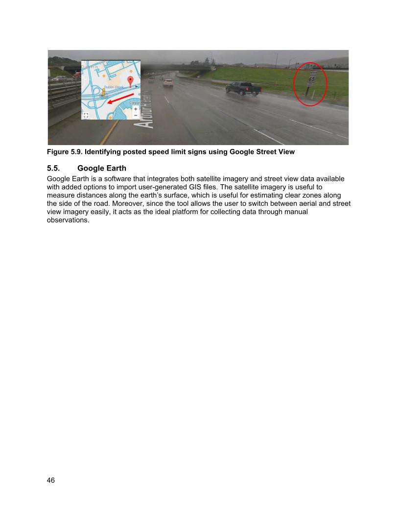
Figure 5.9. Identifying posted speed limit signs using Google Street View
5.5. Google Earth Google Earth is a software that integrates both satellite imagery and street view data available with added options to import user-generated GIS files. The satellite imagery is useful to measure distances along the earth’s surface, which is useful for estimating clear zones along the side of the road. Moreover, since the tool allows the user to switch between aerial and street view imagery easily, it acts as the ideal platform for collecting data through manual observations.
46

6. PILOT STUDY FOR DATA COLLECTION USING EXTERNAL SOURCES
The motivation behind developing pilot manual data collection effort is two-fold: 1. Time-cost estimation: Estimating the time needed to manually collect data elements
using Google Earth/Street View 2. Ground truth: Using street view to obtain accurate, but tedious to collect data, which can
otherwise be estimated through other scalable data sources
Collectively, these two objectives help the research team assess the costs associated with manual data collection using Google Earth/Street View as a feasible methodology for Caltrans for different variables. Based on this approach, the following missing data elements were focused on as part of the pilot study:
1. Time-cost estimation: a. Segments:
Minimum/maximum clear recovery zone (on either side) Center turning lane (none/two-way/one-way) Driveways (count, on either side)
b. Intersections: Crosswalks (unmarked/standard/yellow)
2. Ground truth for other sources: a. Segments (but also applicable for intersections):
Posted speed limit signs (integers (mph), on either side) Elevation (approximately 1/10th PM)
6.1. Sampling methodology for pilot locations To obtain a diverse, representative set of locations, the following variables were considered as part of a factorial design:
• Functional classification of the road (freeway vs arterial) • Urban vs Rural • Two-lane vs multi-lane
In addition to the variables listed above, other supplementary variables were also summarized to ensure additional variation for the purposes of the data collection:
• Design speed variation • Number of intersections
Given the variables under consideration, the TASAS segment and intersection databases were integrated to identify contiguous segments which would satisfy a full factorial design:
• Freeway--Urban--Two-lane • Freeway--Urban--Multi-lane • Freeway--Rural--Two-lane • Freeway--Rural--Multi-lane • Arterial--Urban--Two-lane • Arterial--Urban--Multi-lane • Arterial--Rural--Two-lane • Arterial--Rural--Multi-lane
47

6.2. List of locations for the pilot study Based on the sampling methodology, ~94 miles of segments were identified across 10 contiguous segments as listed in Table 6.1.
Table 6.1. List of locations for the pilot study
Table 6.2 also shows that the pilot study locations are relatively evenly split across the functional class, urban/rural and number of lane categories, thus providing a wide range of conditions under which the manual data collection can be tested.
Table 6.2. Distribution of pilot study locations across different variables of interest DISTRIBUTION ACROSS VARIABLES
Urban/Rural Length (miles)
Functional Class
Length (miles)
Lane Type Length (miles)
Rural 46.053 Arterial 52.035 Multi-lane 44.883
Urban 47.593 Freeway 41.611 Two-lane 48.763
Figure 6.1 shows the locations of the different study locations, which also indicates that the locations are also spread out across different parts of California.
48
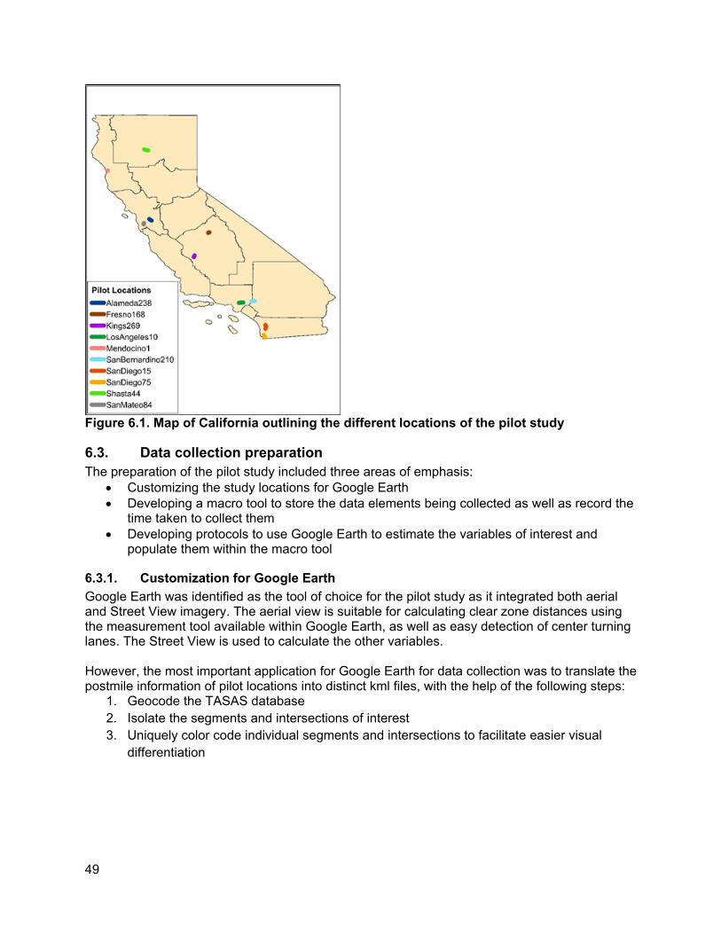
Figure 6.1. Map of California outlining the different locations of the pilot study
6.3. Data collection preparation The preparation of the pilot study included three areas of emphasis:
• Customizing the study locations for Google Earth • Developing a macro tool to store the data elements being collected as well as record the
time taken to collect them • Developing protocols to use Google Earth to estimate the variables of interest and
populate them within the macro tool
6.3.1. Customization for Google Earth Google Earth was identified as the tool of choice for the pilot study as it integrated both aerial and Street View imagery. The aerial view is suitable for calculating clear zone distances using the measurement tool available within Google Earth, as well as easy detection of center turning lanes. The Street View is used to calculate the other variables.
However, the most important application for Google Earth for data collection was to translate the postmile information of pilot locations into distinct kml files, with the help of the following steps:
1. Geocode the TASAS database 2. Isolate the segments and intersections of interest 3. Uniquely color code individual segments and intersections to facilitate easier visual
differentiation
49
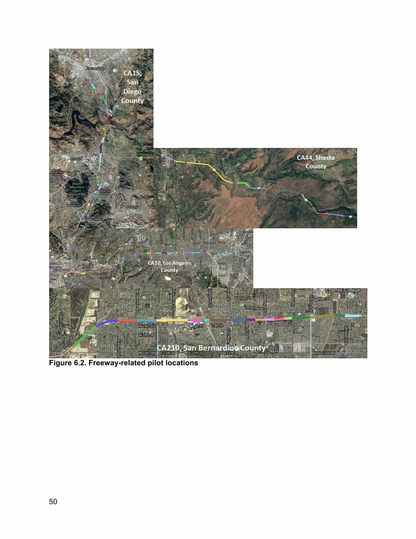
Figure 6.2. Freeway-related pilot locations
50
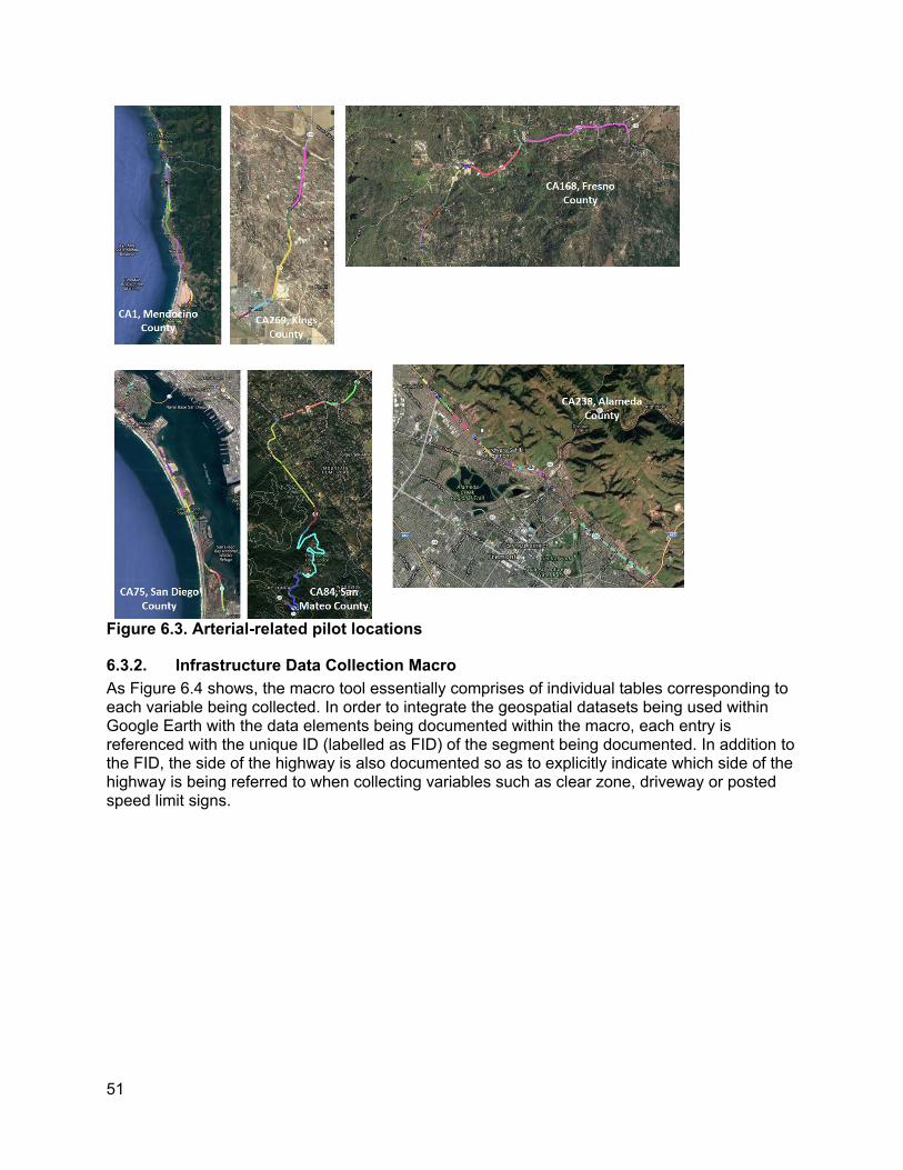
Figure 6.3. Arterial-related pilot locations
6.3.2. Infrastructure Data Collection Macro As Figure 6.4 shows, the macro tool essentially comprises of individual tables corresponding to each variable being collected. In order to integrate the geospatial datasets being used within Google Earth with the data elements being documented within the macro, each entry is referenced with the unique ID (labelled as FID) of the segment being documented. In addition to the FID, the side of the highway is also documented so as to explicitly indicate which side of the highway is being referred to when collecting variables such as clear zone, driveway or posted speed limit signs.
51
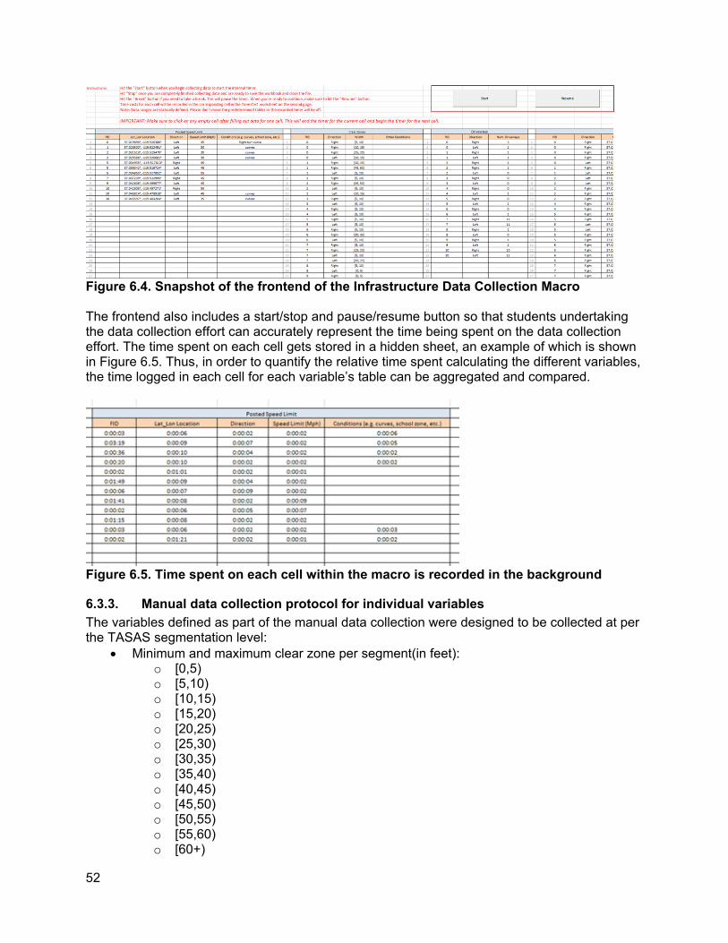
Figure 6.4. Snapshot of the frontend of the Infrastructure Data Collection Macro
The frontend also includes a start/stop and pause/resume button so that students undertaking the data collection effort can accurately represent the time being spent on the data collection effort. The time spent on each cell gets stored in a hidden sheet, an example of which is shown in Figure 6.5. Thus, in order to quantify the relative time spent calculating the different variables, the time logged in each cell for each variable’s table can be aggregated and compared.
Figure 6.5. Time spent on each cell within the macro is recorded in the background
6.3.3. Manual data collection protocol for individual variables The variables defined as part of the manual data collection were designed to be collected at per the TASAS segmentation level:
• Minimum and maximum clear zone per segment(in feet): o [0,5) o [5,10) o [10,15) o [15,20) o [20,25) o [25,30) o [30,35) o [35,40) o [40,45) o [45,50) o [50,55) o [55,60) o [60+)
52
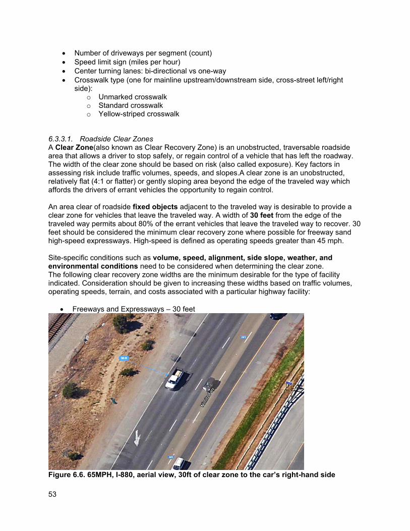
• Number of driveways per segment (count) • Speed limit sign (miles per hour) • Center turning lanes: bi-directional vs one-way • Crosswalk type (one for mainline upstream/downstream side, cross-street left/right
side): o Unmarked crosswalk o Standard crosswalk o Yellow-striped crosswalk
6.3.3.1. Roadside Clear Zones A Clear Zone(also known as Clear Recovery Zone) is an unobstructed, traversable roadside area that allows a driver to stop safely, or regain control of a vehicle that has left the roadway. The width of the clear zone should be based on risk (also called exposure). Key factors in assessing risk include traffic volumes, speeds, and slopes.A clear zone is an unobstructed, relatively flat (4:1 or flatter) or gently sloping area beyond the edge of the traveled way which affords the drivers of errant vehicles the opportunity to regain control.
An area clear of roadside fixed objects adjacent to the traveled way is desirable to provide a clear zone for vehicles that leave the traveled way. A width of 30 feet from the edge of the traveled way permits about 80% of the errant vehicles that leave the traveled way to recover. 30 feet should be considered the minimum clear recovery zone where possible for freeway sand high-speed expressways. High-speed is defined as operating speeds greater than 45 mph.
Site-specific conditions such as volume, speed, alignment, side slope, weather, and environmental conditions need to be considered when determining the clear zone. The following clear recovery zone widths are the minimum desirable for the type of facility indicated. Consideration should be given to increasing these widths based on traffic volumes, operating speeds, terrain, and costs associated with a particular highway facility:
• Freeways and Expressways – 30 feet
Figure 6.6. 65MPH, I-880, aerial view, 30ft of clear zone to the car’s right-hand side
53
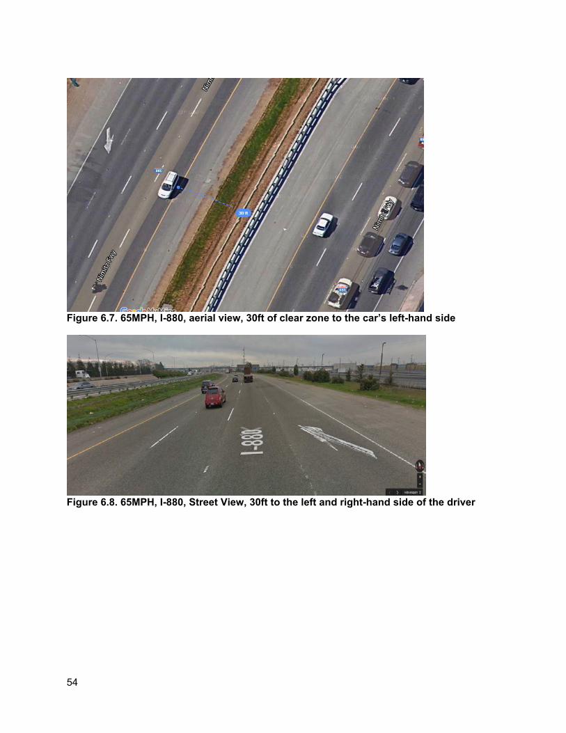
Figure 6.7. 65MPH, I-880, aerial view, 30ft of clear zone to the car’s left-hand side
Figure 6.8. 65MPH, I-880, Street View, 30ft to the left and right-hand side of the driver
54
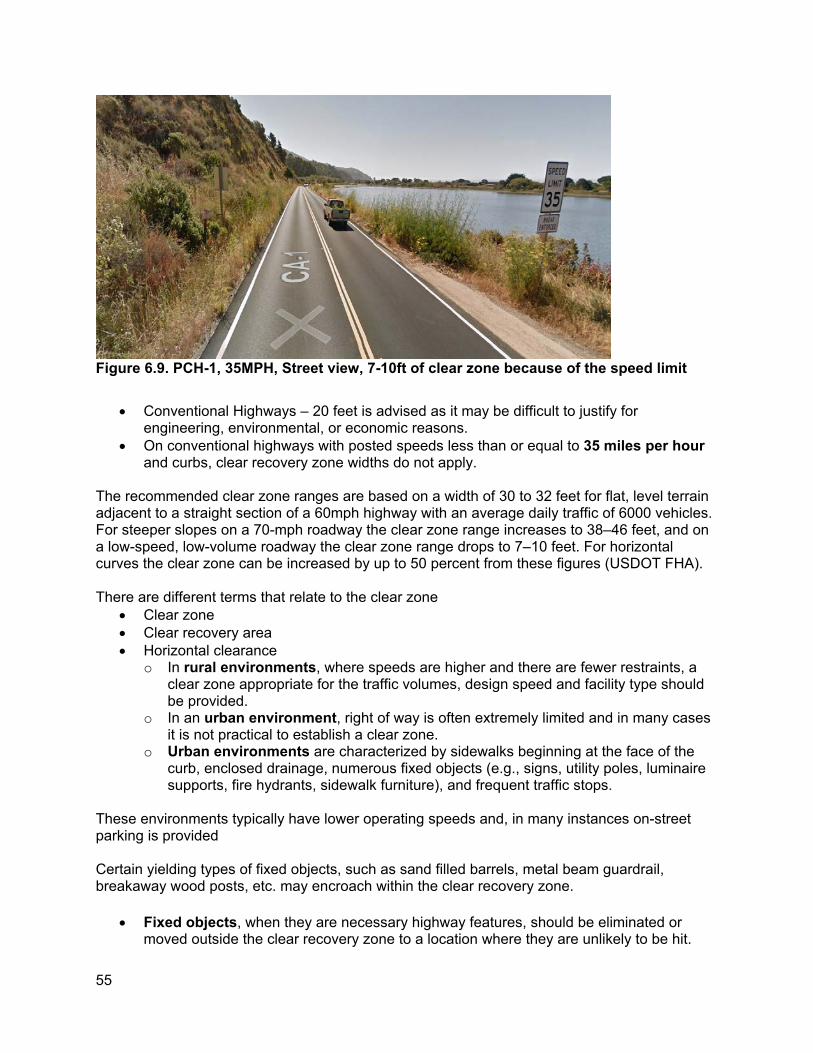
Figure 6.9. PCH-1, 35MPH, Street view, 7-10ft of clear zone because of the speed limit
• Conventional Highways – 20 feet is advised as it may be difficult to justify for engineering, environmental, or economic reasons.
• On conventional highways with posted speeds less than or equal to 35 miles per hour and curbs, clear recovery zone widths do not apply.
The recommended clear zone ranges are based on a width of 30 to 32 feet for flat, level terrain adjacent to a straight section of a 60mph highway with an average daily traffic of 6000 vehicles. For steeper slopes on a 70-mph roadway the clear zone range increases to 38–46 feet, and on a low-speed, low-volume roadway the clear zone range drops to 7–10 feet. For horizontal curves the clear zone can be increased by up to 50 percent from these figures (USDOT FHA).
There are different terms that relate to the clear zone • Clear zone • Clear recovery area • Horizontal clearance
o In rural environments, where speeds are higher and there are fewer restraints, a clear zone appropriate for the traffic volumes, design speed and facility type should be provided.
o In an urban environment, right of way is often extremely limited and in many cases it is not practical to establish a clear zone.
o Urban environments are characterized by sidewalks beginning at the face of the curb, enclosed drainage, numerous fixed objects (e.g., signs, utility poles, luminaire supports, fire hydrants, sidewalk furniture), and frequent traffic stops.
These environments typically have lower operating speeds and, in many instances on-street parking is provided
Certain yielding types of fixed objects, such as sand filled barrels, metal beam guardrail, breakaway wood posts, etc. may encroach within the clear recovery zone.
• Fixed objects, when they are necessary highway features, should be eliminated or moved outside the clear recovery zone to a location where they are unlikely to be hit.
55
• If necessary highway features such as sign posts or light standards cannot be eliminated or moved outside the clear recovery zone, they should be made yielding with a breakaway feature.
• If a fixed object, when they are necessary highway features, cannot be eliminated, moved outside the clear recovery zone, or modified to be made yielding, it should be shielded by guardrail.
Fixed objects that cannot be moved out of the clear zone should be considered for breakaway treatment. These include but are not limited to the following:
• Light standards • Ground-mounted sign supports • Mailbox supports • Call boxes • Chain control signs
If it is not practical to eliminate, relocate, or make a fixed object breakaway, it should be considered for shielding. All traffic safety systems used to shield fixed objects are also fixed objects.
Discretionary fixed objects are features or facilities that are not necessary for the safety, maintenance or operation of the highway, but may enhance livability and sustainability. These may include, but are not limited to, transportation art, gateway monuments, solar panels, and memorial/historical plaques or markers.
Using this background about clear zones, the Google Earth and macro can be used for estimating the clear zones as follows:
1. The first step when attempting to find the minimum and maximum distance of clear zones is have a set of established points to follow. Once thoselat-long/elevation /intersection points are established, the process can begin.
2. One method that can be used is Google Earth; this is a more efficient way of identifying the length of clear zones.
3. To use Google Earth,it must be downloaded (the online version will not suffice, so the actual software program must be downloaded). Admin privileges are required if the program is not already downloaded.
4. Log in to Google Earth so that the work can be stored and shared with others. 5. Open Google Earth and use the entire primary screen, on the secondary screen have
the Macro Tool open. There are different ways to export KML files onto Google Earth: import the segment/elevation/intersection files for the appropriate highway you will be collecting data for.
6. The screen shot below shows how the screen should appear when read to start.
56
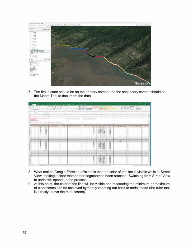
7. The first picture should be on the primary screen and the secondary screen should be the Macro Tool to document the data.
8. What makes Google Earth so efficient is that the color of the line is visible while in Street View, making it clear thatanother segmenthas been reached. Switching from Street View to aerial will speed up the process.
9. At this point, the color of the line will be visible and measuring the minimum or maximum of clear zones can be achieved bymerely zooming out back to aerial mode (the ruler tool is directly above the map screen).
57
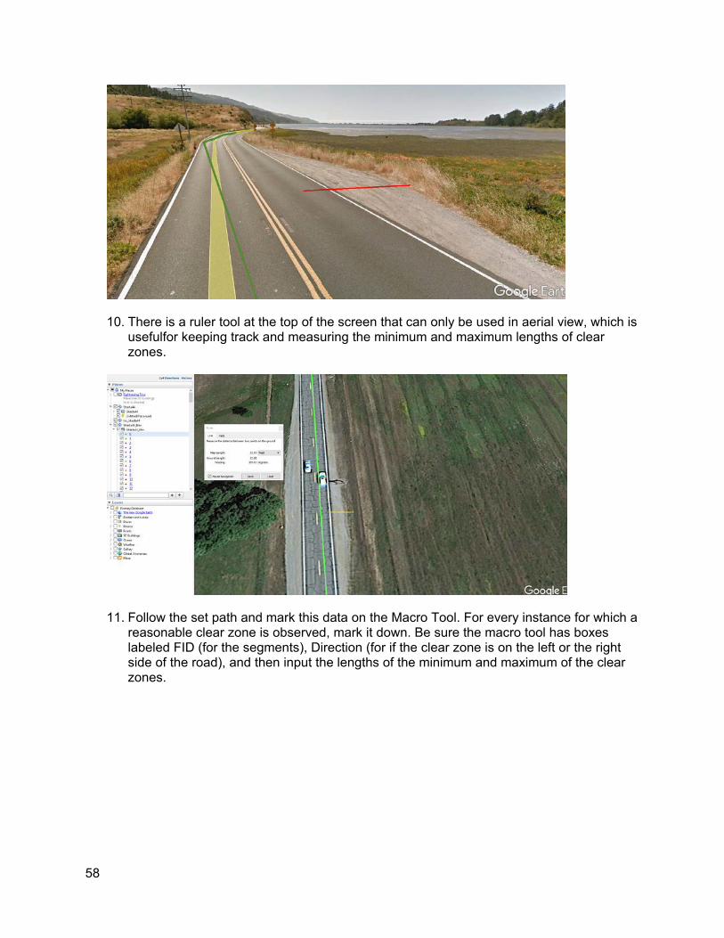
10. There is a ruler tool at the top of the screen that can only be used in aerial view, which is usefulfor keeping track and measuring the minimum and maximum lengths of clear zones.
11. Follow the set path and mark this data on the Macro Tool. For every instance for which a reasonable clear zone is observed, mark it down. Be sure the macro tool has boxes labeled FID (for the segments), Direction (for if the clear zone is on the left or the right side of the road), and then input the lengths of the minimum and maximum of the clear zones.
58
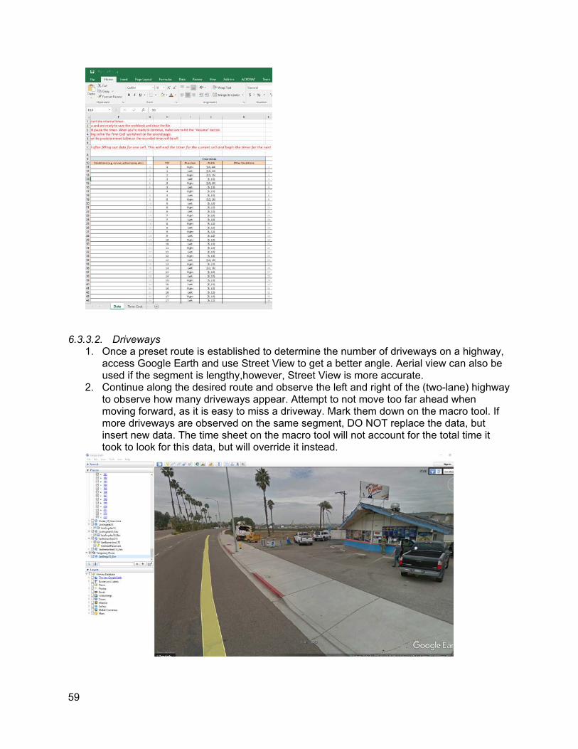
6.3.3.2. Driveways 1. Once a preset route is established to determine the number of driveways on a highway,
access Google Earth and use Street View to get a better angle. Aerial view can also be used if the segment is lengthy,however, Street View is more accurate.
2. Continue along the desired route and observe the left and right of the (two-lane) highway to observe how many driveways appear. Attempt to not move too far ahead when moving forward, as it is easy to miss a driveway. Mark them down on the macro tool. If more driveways are observed on the same segment, DO NOT replace the data, but insert new data. The time sheet on the macro tool will not account for the total time it took to look for this data, but will override it instead.
59
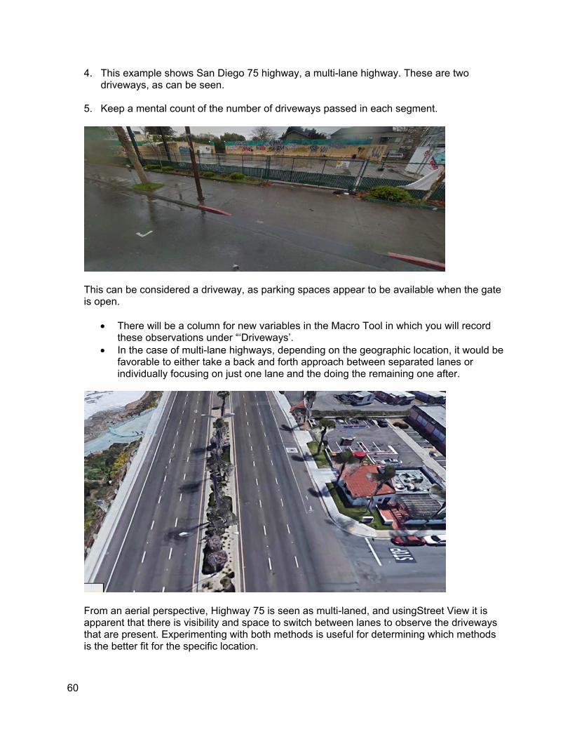
4. This example shows San Diego 75 highway, a multi-lane highway. These are two driveways, as can be seen.
5. Keep a mental count of the number of driveways passed in each segment.
This can be considered a driveway, as parking spaces appear to be available when the gate is open.
• There will be a column for new variables in the Macro Tool in which you will record these observations under “‘Driveways’.
• In the case of multi-lane highways, depending on the geographic location, it would be favorable to either take a back and forth approach between separated lanes or individually focusing on just one lane and the doing the remaining one after.
From an aerial perspective, Highway 75 is seen as multi-laned, and usingStreet View it is apparent that there is visibility and space to switch between lanes to observe the driveways that are present. Experimenting with both methods is useful for determining which methods is the better fit for the specific location.
60
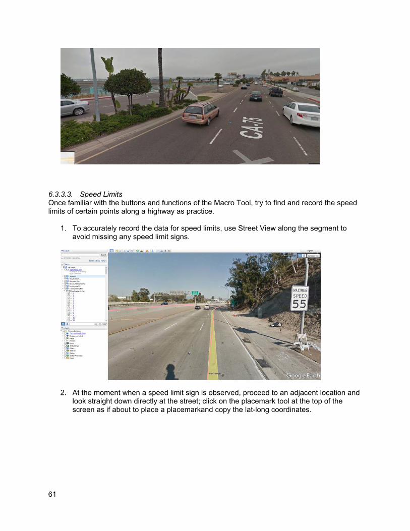
6.3.3.3. Speed Limits Once familiar with the buttons and functions of the Macro Tool, try to find and record the speed limits of certain points along a highway as practice.
1. To accurately record the data for speed limits, use Street View along the segment to avoid missing any speed limit signs.
2. At the moment when a speed limit sign is observed, proceed to an adjacent location and look straight down directly at the street; click on the placemark tool at the top of the screen as if about to place a placemarkand copy the lat-long coordinates.
61
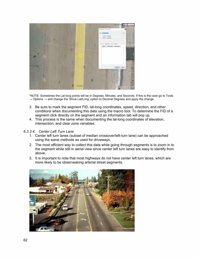
*NOTE: Sometimes the Lat-long points will be in Degrees, Minutes, and Seconds. If this is the case go to Tools → Options → and change the ‘Show Lat/Long’ option to Decimal Degrees and apply the change.
3. Be sure to mark the segment FID, lat-long coordinates, speed, direction, and other conditions when documenting this data using the macro tool. To determine the FID of a segment click directly on the segment and an information tab will pop up.
4. This process is the same when documenting the lat-long coordinates of elevation, intersection, and clear zone variables.
6.3.3.4. Center Left Turn Lane 1. Center left turn lanes (subset of median crossover/left-turn lane) can be approached
using the same methods as used for driveways. 2. The most efficient way to collect this data while going through segments is to zoom in to
the segment while still in aerial view since center left turn lanes are easy to identify from above.
3. It is important to note that most highways do not have center left turn lanes, which are more likely to be observealong arterial street segments.
62

7. PILOT RESULTS
7.1. Summary statistics of variables collected across different projects Table 7.1 summarizes the pilot data collection time estimates for the different pilot locations. As the results reveal, the most time consuming variables correspond to elevation data, followed by clear zones and posted speed limits. However, it is important to note that both elevation and speed limit estimates were collected primarily as ground truth for assessing alternate data sources. In comparison, manual data collection is the sole data source for roadside clearzone width, center left turn lane, and driveway counts that was identified as part of this project. Thus, the unit time-costs, as defined by minutes/mile/direction, are shown in Table 7.1.
Table 7.1. Summary of the relative time spent collecting different variables
county routex length (in PM)
Time (in minutes)
Elevation (in
minutes)
Clear Zone (in minutes)
Posted Speed
Limit (in minutes)
Driveways (in
minutes)
Crosswalks (in minutes)
Center Turning
Lanes (in minutes)
Minutes/ mile/dire
ction
Minutes/mil e/direction (excluding Elevation)
Minutes/mil e/direction (excluding Elevation and Speed
Limit) Shasta 44 10.24 115.3 54% 14% 9% 6% 14% 4% 5.63 2.61 2.13
Los Angeles 10 11.09 203.0 52% 28% 17% 3% 0% 0% 9.15 4.40 2.86 San Diego 15 11.97 150.5 61% 36% 3% 0% 0% 0% 6.29 2.43 2.27
San Bernardino 210 8.311 90.7 55% 19% 26% 0% 0% 0% 5.45 2.48 1.05 Mendocino 1 15.63 176.6 42% 33% 8% 10% 7% 0% 5.65 3.27 2.82 San Mateo 84 6.493 96.7 39% 12% 10% 24% 15% 0% 7.44 4.53 3.80
Kings 269 5.31 90.1 35% 33% 2% 15% 13% 2% 8.48 5.47 5.32 Fresno 168 8.213 111.1 39% 17% 13% 23% 7% 0% 6.76 4.10 3.21
San Diego 75 8.976 86.1 49% 20% 7% 12% 12% 1% 4.80 2.44 2.12 Alameda 238 7.413 263.2 39% 15% 13% 24% 9% 1% 17.75 10.84 8.62
7.2. Time-cost estimation Based on the distribution of the time-cost estimates provided in Table 7.1, the average unit time-cost estimates (minutes/mile/direction) for urban/rural and freeway/arterial classification is shown in Table 7.2.The findings reveal that the time required to collect variables for arterial roadways in urban regions is the highest.
Table 7.2. Summary of the average unit time-cost estimates aggregated by differentroadway types
Roadway Type Ave.
Minutes/mile/direction Ave. Minutes/mile/direction
(excluding Elevation)
Minutes/mile/direction (excluding Elevation and Speed
Limit) Arterial & Rural 6.03 3.56 2.96 Arterial & Urban 9.51 5.70 4.82 Freeway & Rural 5.98 2.52 2.20 Freeway & Urban 7.57 3.57 2.08
Finally, based on the estimates provided in Table 7.2, the time required to collect the variables across the entire state highway system can be computed. The estimates shown in Table 7.3 indicate that it takes around 3772 hours to collect all the variable across the state highway system. However, when excluding the collection of elevation data, the estimate reduces to 1958 hours. Lastly, when excluding both elevation and post speed limit variables, the time-cost estimate is 1534 hours.
63
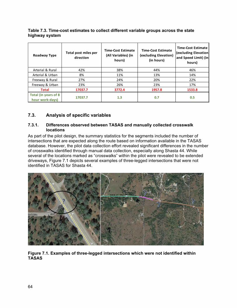
Table 7.3. Time-cost estimates to collect different variable groups across the state highway system
Roadway Type Total post miles per
direction
Time-Cost Estimate (All Variables) (in
hours)
Time-Cost Estimate (excluding Elevation)
(in hours)
Time-Cost Estimate (excluding Elevation and Speed Limit) (in
hours)
Arterial & Rural 42% 38% 44% 46% Arterial & Urban 8% 11% 13% 14% Freeway & Rural 27% 24% 20% 22% Freeway & Urban 23% 26% 23% 17%
Total 17037.7 3772.4 1957.8 1533.8 Total (in years of 8 hour work-days) 17037.7 1.3 0.7 0.5
7.3. Analysis of specific variables
7.3.1. Differences observed between TASAS and manually collected crosswalk locations
As part of the pilot design, the summary statistics for the segments included the number of intersections that are expected along the route based on information available in the TASAS database. However, the pilot data collection effort revealed significant differences in the number of crosswalks identified through manual data collection, especially along Shasta 44. While several of the locations marked as “crosswalks” within the pilot were revealed to be extended driveways, Figure 7.1 depicts several examples of three-legged intersections that were not identified in TASAS for Shasta 44.
Figure 7.1. Examples of three-legged intersections which were not identified within TASAS
64
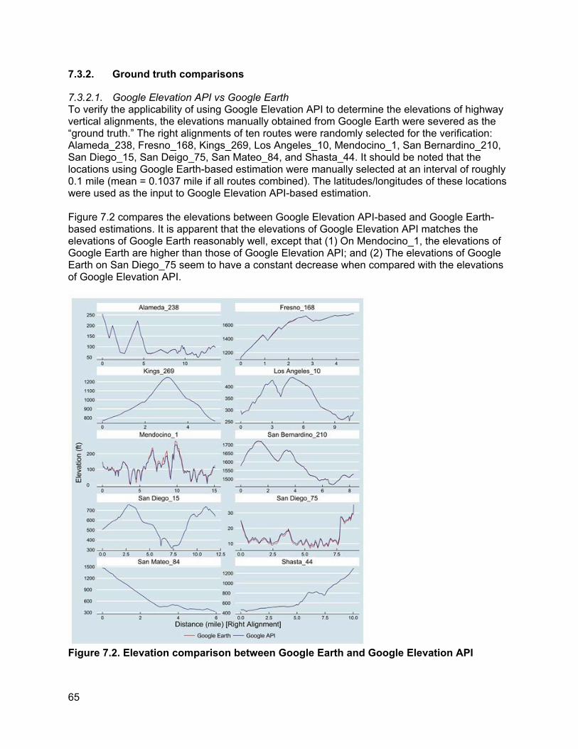
7.3.2. Ground truth comparisons
7.3.2.1. Google Elevation API vs Google Earth To verify the applicability of using Google Elevation API to determine the elevations of highway vertical alignments, the elevations manually obtained from Google Earth were severed as the “ground truth.” The right alignments of ten routes were randomly selected for the verification: Alameda_238, Fresno_168, Kings_269, Los Angeles_10, Mendocino_1, San Bernardino_210, San Diego_15, San Deigo_75, San Mateo_84, and Shasta_44. It should be noted that the locations using Google Earth-based estimation were manually selected at an interval of roughly 0.1 mile (mean = 0.1037 mile if all routes combined). The latitudes/longitudes of these locations were used as the input to Google Elevation API-based estimation.
Figure 7.2 compares the elevations between Google Elevation API-based and Google Earth-based estimations. It is apparent that the elevations of Google Elevation API matches the elevations of Google Earth reasonably well, except that (1) On Mendocino_1, the elevations of Google Earth are higher than those of Google Elevation API; and (2) The elevations of Google Earth on San Diego_75 seem to have a constant decrease when compared with the elevations of Google Elevation API.
Figure 7.2. Elevation comparison between Google Earth and Google Elevation API
65
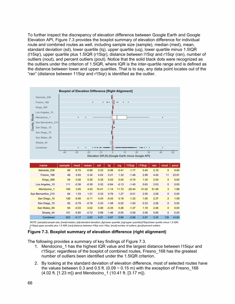
To further inspect the discrepancy of elevation difference between Google Earth and Google Elevation API, Figure 7.3 provides the boxplot summary of elevation difference for individual route and combined routes as well, including sample size (sample), median (med), mean, standard deviation (sd), lower quartile (lq), upper quartile (uq), lower quartile minus 1.5IQR (l15iqr), upper quartile plus 1.5IQR (r15iqr), distance between l15iqr and r15iqr (ran), number of outliers (nout), and percent outliers (pout). Notice that the solid black dots were recognized as the outliers under the criterion of 1.5IQR, where IQR is the inter-quartile range and is defined as the distance between lower and upper quartiles. That is to say, any data point locates out of the “ran” (distance between 115iqr and r15iqr) is identified as the outlier.
Figure 7.3. Boxplot summary of elevation difference (right alignment)
The following provides a summary of key findings of Figure 7.3. 1. Mendocino_1 has the highest IQR value and the largest distance between l15iqur and
r15iqur; regardless of the boxplot of combined routes, Fresno_168 has the greatest number of outliers been identified under the 1.5IQR criterion.
2. By looking at the standard deviation of elevation difference, most of selected routes have the values between 0.3 and 0.5 ft. (0.09 ~ 0.15 m) with the exception of Fresno_168 (4.02 ft. [1.23 m]) and Mendocino_1 (10.41 ft. [3.17 m]).
66
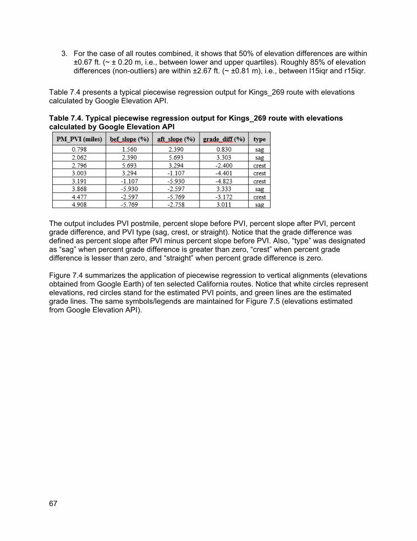
3. For the case of all routes combined, it shows that 50% of elevation differences are within ±0.67 ft. (~ ± 0.20 m, i.e., between lower and upper quartiles). Roughly 85% of elevation differences (non-outliers) are within ±2.67 ft. (~ ±0.81 m), i.e., between l15iqr and r15iqr.
Table 7.4 presents a typical piecewise regression output for Kings_269 route with elevations calculated by Google Elevation API.
Table 7.4. Typical piecewise regression output for Kings_269 route with elevations calculated by Google Elevation API
The output includes PVI postmile, percent slope before PVI, percent slope after PVI, percent grade difference, and PVI type (sag, crest, or straight). Notice that the grade difference was defined as percent slope after PVI minus percent slope before PVI. Also, “type” was designated as “sag” when percent grade difference is greater than zero, “crest” when percent grade difference is lesser than zero, and “straight” when percent grade difference is zero.
Figure 7.4 summarizes the application of piecewise regression to vertical alignments (elevations obtained from Google Earth) of ten selected California routes. Notice that white circles represent elevations, red circles stand for the estimated PVI points, and green lines are the estimated grade lines. The same symbols/legends are maintained for Figure 7.5 (elevations estimated from Google Elevation API).
67
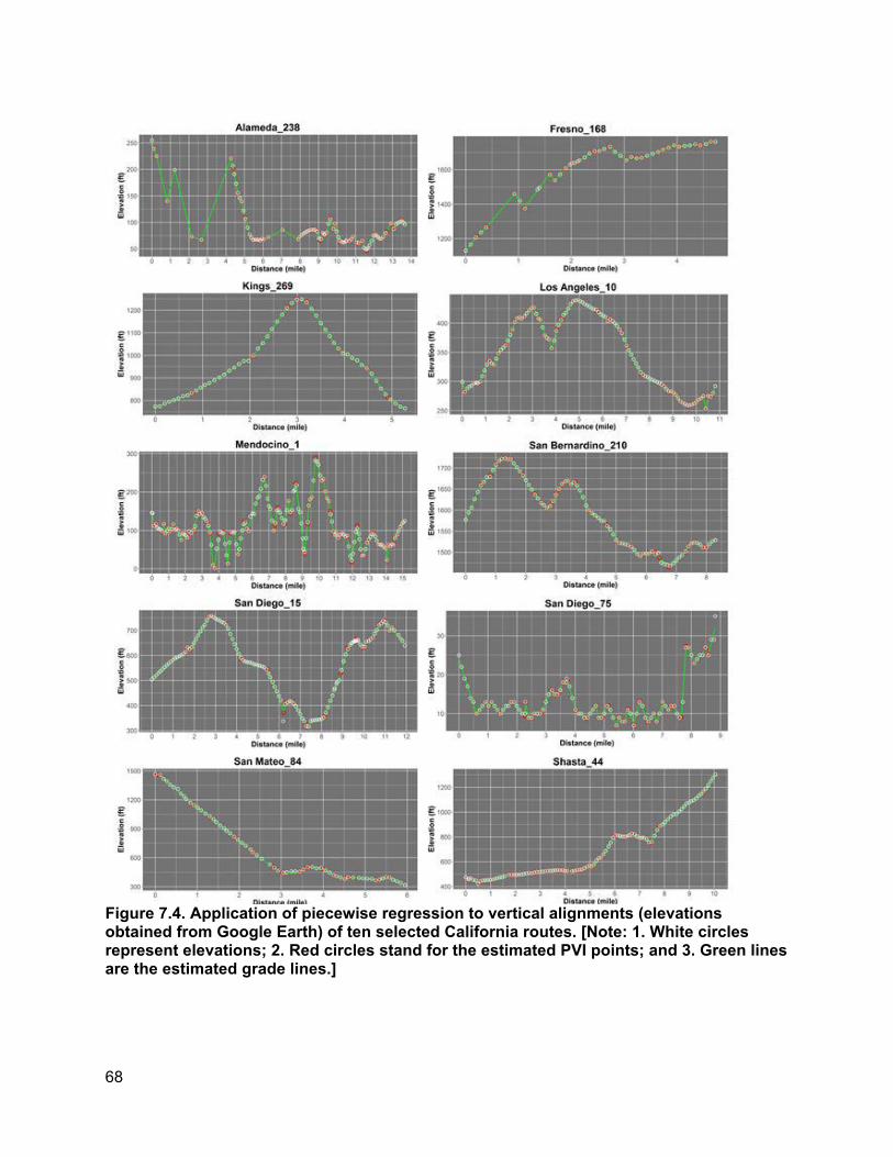
Figure 7.4. Application of piecewise regression to vertical alignments (elevations obtained from Google Earth) of ten selected California routes. [Note: 1. White circles represent elevations; 2. Red circles stand for the estimated PVI points; and 3. Green lines are the estimated grade lines.]
68
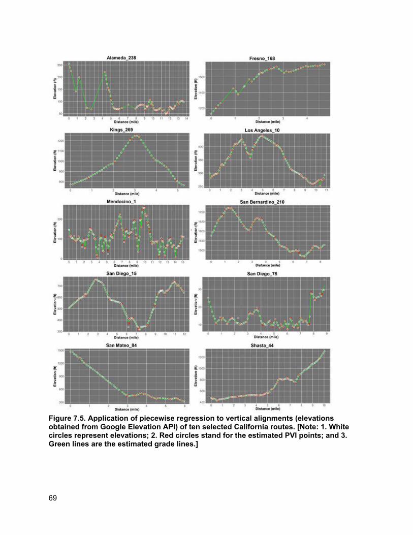
Figure 7.5. Application of piecewise regression to vertical alignments (elevations obtained from Google Elevation API) of ten selected California routes. [Note: 1. White circles represent elevations; 2. Red circles stand for the estimated PVI points; and 3. Green lines are the estimated grade lines.]
69
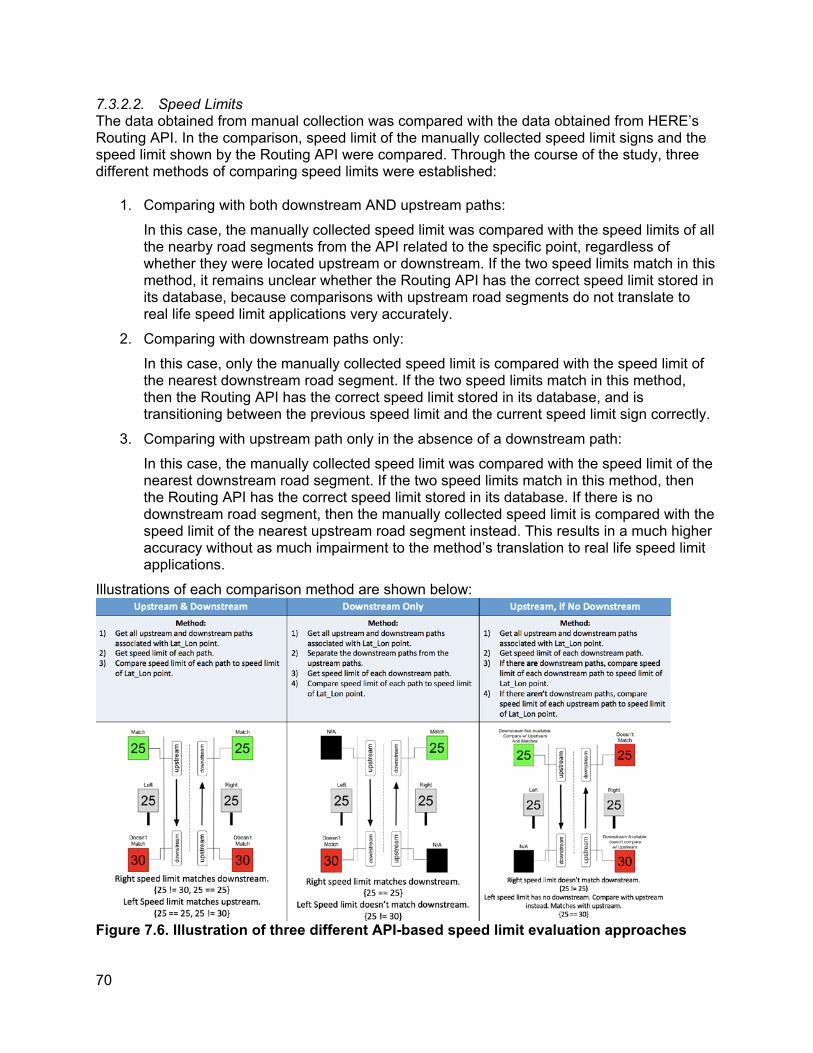
7.3.2.2. Speed Limits The data obtained from manual collection was compared with the data obtained from HERE’s Routing API. In the comparison, speed limit of the manually collected speed limit signs and the speed limit shown by the Routing API were compared. Through the course of the study, three different methods of comparing speed limits were established:
1. Comparing with both downstream AND upstream paths: In this case, the manually collected speed limit was compared with the speed limits of all the nearby road segments from the API related to the specific point, regardless of whether they were located upstream or downstream. If the two speed limits match in this method, it remains unclear whether the Routing API has the correct speed limit stored in its database, because comparisons with upstream road segments do not translate to real life speed limit applications very accurately.
2. Comparing with downstream paths only: In this case, only the manually collected speed limit is compared with the speed limit of the nearest downstream road segment. If the two speed limits match in this method, then the Routing API has the correct speed limit stored in its database, and is transitioning between the previous speed limit and the current speed limit sign correctly.
3. Comparing with upstream path only in the absence of a downstream path: In this case, the manually collected speed limit was compared with the speed limit of the nearest downstream road segment. If the two speed limits match in this method, then the Routing API has the correct speed limit stored in its database. If there is no downstream road segment, then the manually collected speed limit is compared with the speed limit of the nearest upstream road segment instead. This results in a much higher accuracy without as much impairment to the method’s translation to real life speed limit applications.
Illustrations of each comparison method are shown below:
Figure 7.6. Illustration of three different API-based speed limit evaluation approaches
70
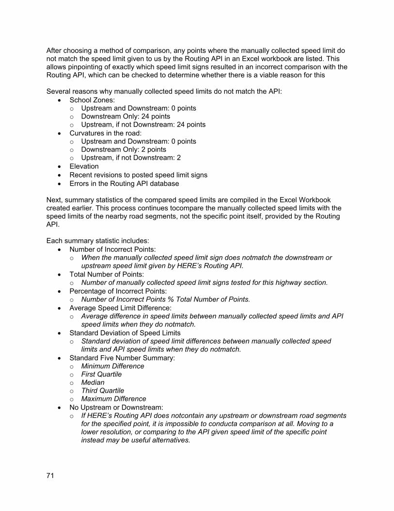
After choosing a method of comparison, any points where the manually collected speed limit do not match the speed limit given to us by the Routing API in an Excel workbook are listed. This allows pinpointing of exactly which speed limit signs resulted in an incorrect comparison with the Routing API, which can be checked to determine whether there is a viable reason for this
Several reasons why manually collected speed limits do not match the API: • School Zones:
o Upstream and Downstream: 0 points o Downstream Only: 24 points o Upstream, if not Downstream: 24 points
• Curvatures in the road: o Upstream and Downstream: 0 points o Downstream Only: 2 points o Upstream, if not Downstream: 2
• Elevation • Recent revisions to posted speed limit signs • Errors in the Routing API database
Next, summary statistics of the compared speed limits are compiled in the Excel Workbook created earlier. This process continues tocompare the manually collected speed limits with the speed limits of the nearby road segments, not the specific point itself, provided by the Routing API.
Each summary statistic includes: • Number of Incorrect Points:
o When the manually collected speed limit sign does notmatch the downstream or upstream speed limit given by HERE’s Routing API.
• Total Number of Points: o Number of manually collected speed limit signs tested for this highway section.
• Percentage of Incorrect Points: o Number of Incorrect Points % Total Number of Points.
• Average Speed Limit Difference: o Average difference in speed limits between manually collected speed limits and API
speed limits when they do notmatch. • Standard Deviation of Speed Limits
o Standard deviation of speed limit differences between manually collected speed limits and API speed limits when they do notmatch.
• Standard Five Number Summary: o Minimum Difference o First Quartile o Median o Third Quartile o Maximum Difference
• No Upstream or Downstream: o If HERE’s Routing API does notcontain any upstream or downstream road segments
for the specified point, it is impossible to conducta comparison at all. Moving to a lower resolution, or comparing to the API given speed limit of the specific point instead may be useful alternatives.
71
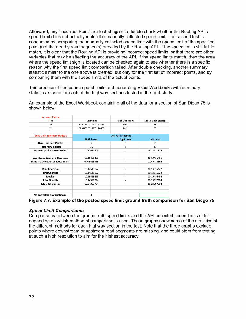
Afterward, any “Incorrect Point” are tested again to double check whether the Routing API’s speed limit does not actually match the manually collected speed limit. The second test is conducted by comparing the manually collected speed limit with the speed limit of the specified point (not the nearby road segments) provided by the Routing API. If the speed limits still fail to match, it is clear that the Routing API is providing incorrect speed limits, or that there are other variables that may be affecting the accuracy of the API. If the speed limits match, then the area where the speed limit sign is located can be checked again to see whether there is a specific reason why the first speed limit comparison failed. After double checking, another summary statistic similar to the one above is created, but only for the first set of incorrect points, and by comparing them with the speed limits of the actual points.
This process of comparing speed limits and generating Excel Workbooks with summary statistics is used for each of the highway sections tested in the pilot study.
An example of the Excel Workbook containing all of the data for a section of San Diego 75 is shown below:
Figure 7.7. Example of the posted speed limit ground truth comparison for San Diego 75
Speed Limit Comparisons Comparisons between the ground truth speed limits and the API collected speed limits differ depending on which method of comparison is used. These graphs show some of the statistics of the different methods for each highway section in the test. Note that the three graphs exclude points where downstream or upstream road segments are missing, and could stem from testing at such a high resolution to aim for the highest accuracy.
72
Figure 7.8. Box plots showing distribution of speed limit estimation error for different approaches
Upstream & Downstream: • Curve Errors: 0 • School Zone Errors: 0 • Total Errors: 20 • Number of No Downstream & Upstream: 86
Downstream Only: • Curve Errors: 24 • School Zone Errors: 2 • Total Errors: 37 • Number of No Downstream: 56
Upstream, if not Downstream: • Curve Errors: 24 • School Zone Errors: 2 • Total Errors: 37 • Number of No Downstream & Upstream: 53
The upstream & downstream method demonstrates the greatest accuracy, but this method does not provide into how new locations can be populated. The downstream only method shows the lowest accuracy, but this accuracy is improved by selection upstream speed limit in the absence of any downstream points. Moreover, the accuracy estimates provided above are significantly increased when ignoring curve-related suggested speed limits since these are only suggest speed limited.
In summary, while the speed limit API provides a scalable approach to populate speed limit, Google Street View-based manual data collection allows documenting both regulatory as well as suggested speed limit information. Moreover, the identification of speed limit signs can also be categorized as fixed object information.
73
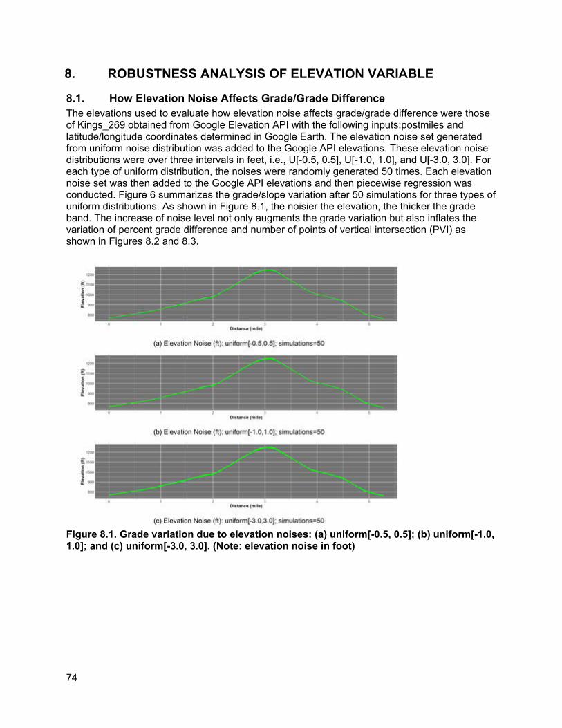
8. ROBUSTNESS ANALYSIS OF ELEVATION VARIABLE
8.1. How Elevation Noise Affects Grade/Grade Difference The elevations used to evaluate how elevation noise affects grade/grade difference were those of Kings_269 obtained from Google Elevation API with the following inputs:postmiles and latitude/longitude coordinates determined in Google Earth. The elevation noise set generated from uniform noise distribution was added to the Google API elevations. These elevation noise distributions were over three intervals in feet, i.e., U[-0.5, 0.5], U[-1.0, 1.0], and U[-3.0, 3.0]. For each type of uniform distribution, the noises were randomly generated 50 times. Each elevation noise set was then added to the Google API elevations and then piecewise regression was conducted. Figure 6 summarizes the grade/slope variation after 50 simulations for three types of uniform distributions. As shown in Figure 8.1, the noisier the elevation, the thicker the grade band. The increase of noise level not only augments the grade variation but also inflates the variation of percent grade difference and number of points of vertical intersection (PVI) as shown in Figures 8.2 and 8.3.
Figure 8.1. Grade variation due to elevation noises: (a) uniform[-0.5, 0.5]; (b) uniform[-1.0, 1.0]; and (c) uniform[-3.0, 3.0]. (Note: elevation noise in foot)
74
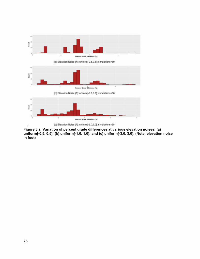
Figure 8.2. Variation of percent grade differences at various elevation noises: (a)uniform[-0.5, 0.5]; (b) uniform[-1.0, 1.0]; and (c) uniform[-3.0, 3.0]. (Note: elevation noise in foot)
75
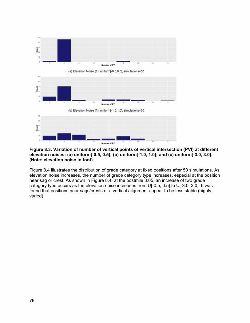
Figure 8.3. Variation of number of vertical points of vertical intersection (PVI) at differentelevation noises: (a) uniform[-0.5, 0.5]; (b) uniform[-1.0, 1.0]; and (c) uniform[-3.0, 3.0]. (Note: elevation noise in foot)
Figure 8.4 illustrates the distribution of grade category at fixed positions after 50 simulations. As elevation noise increases, the number of grade category type increases, especial at the position near sag or crest. As shown in Figure 8.4, at the postmile 3.05, an increase of two grade category type occurs as the elevation noise increases from U[-0.5, 0.5] to U[-3.0, 3.0]. It was found that positions near sags/crests of a vertical alignment appear to be less stable (highly varied).
76
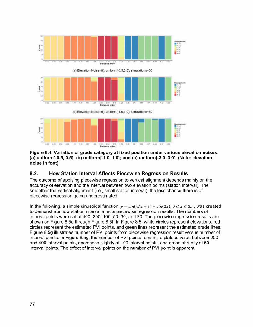
Figure 8.4. Variation of grade category at fixed position under various elevation noises: (a) uniform[-0.5, 0.5]; (b) uniform[-1.0, 1.0]; and (c) uniform[-3.0, 3.0]. (Note: elevation noise in foot)
8.2. How Station Interval Affects Piecewise Regression Results The outcome of applying piecewise regression to vertical alignment depends mainly on the accuracy of elevation and the interval between two elevation points (station interval). The smoother the vertical alignment (i.e., small station interval), the less chance there is of piecewise regression going underestimated.
In the following, a simple sinusoidal function, 𝑦𝑦 = 𝑠𝑠𝑠𝑠𝑠𝑠(𝑥𝑥⁄2 + 5) + 𝑠𝑠𝑠𝑠𝑠𝑠(2𝑥𝑥), 0 ≤ 𝑥𝑥 ≤ 3𝜋𝜋 , was created to demonstrate how station interval affects piecewise regression results. The numbers of interval points were set at 400, 200, 100, 50, 30, and 20. The piecewise regression results are shown on Figure 8.5a through Figure 8.5f. In Figure 8.5, white circles represent elevations, red circles represent the estimated PVI points, and green lines represent the estimated grade lines. Figure 8.5g illustrates number of PVI points from piecewise regression result versus number of interval points. In Figure 8.5g, the number of PVI points remains a plateau value between 200 and 400 interval points, decreases slightly at 100 interval points, and drops abruptly at 50 interval points. The effect of interval points on the number of PVI point is apparent.
77
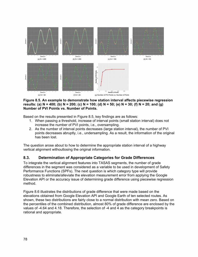
Figure 8.5. An example to demonstrate how station interval affects piecewise regression results: (a) N = 400; (b) N = 200; (c) N = 100; (d) N = 50; (e) N = 30; (f) N = 20; and (g)Number of PVI Points vs. Number of Points.
Based on the results presented in Figure 8.5, key findings are as follows: 1. When passing a threshold, increase of interval points (small station interval) does not
increase the number of PVI points, i.e., oversampling. 2. As the number of interval points decreases (large station interval), the number of PVI
points decreases abruptly, i.e., undersampling. As a result, the information of the original has been lost.
The question arose about to how to determine the appropriate station interval of a highway vertical alignment withoutlosing the original information.
8.3. Determination of Appropriate Categories for Grade Differences To integrate the vertical alignment features into TASAS segments, the number of grade differences in the segment was considered as a variable to be used in development of Safety Performance Functions (SPFs). The next question is which category type will provide robustness to eliminate/alleviate the elevation measurement error from applying the Google Elevation API or the accuracy issue of determining grade difference using piecewise regression method.
Figure 8.6 illustrates the distributions of grade difference that were made based on the elevations obtained from Google Elevation API and Google Earth of ten selected routes. As shown, these two distributions are fairly close to a normal distribution with mean zero. Based on the percentiles of the combined distribution, almost 80% of grade difference are enclosed by the values of -4.64 and 4.18. Therefore, the selection of -4 and 4 as the category breakpoints is rational and appropriate.
78

Figure 8.6. Grade difference distribution for both Google Earth and Google Elevation API. [Note: the percentiles shown were based on the combined grade difference values ofGoogle Earth and Google Elevaton API.]
Three percent grade difference category types, Cat1 (-Inf, -4, -2, 0, 2, 4, Inf), Cat2 (-Inf, -4, 0, 4, Inf), and Cat3 (-Inf, -4, 4, Inf), were selected to inspect the category robustness. The category type (-Inf, -4, -2, 0, 2, 4, Inf) includes six categories, (-Inf, -4], (-4, -2], (-2, 0], (0, 2], (2, 4], and (4, Inf). Notice that “Inf” stands for positive infinite number and “-Inf” represents negative infinite number. Also, notice that the category type (-Inf, -4, 4, Inf) does not include zero as the breakpoint; in other words, this category type cannot differentiate whether the grade difference is sag, crest, or straight when the values of grade difference are in the interval of -4 and 4.
The piecewise regression output (listed in Table 7.4)provides the PVI postmile location and its corresponding percent grade difference. Accordingly, the percent grade differences estimated based on the elevations of Google Elevation API and Google Earth can be assigned to appropriate categories of the three category types. Hence, when plot grade difference category of a specified category type versus postmile in the form of step chart, it will construct a “grade difference pattern.”
In the following, for ten selected routes, Figures 8.7 through 8.9 compare the pattern matching between Google Elevation API and Google Earth for three category types (-Inf, -4, -2, 0, 2, 4, Inf), (-Inf, -4, 0, 4, Inf), and (-Inf, -4, 4, Inf) respectively. Notice that in those figures, the pattern of Google Earth was constructed using colored lines and colored empty circles; the pattern of Google Elevation API was built with white lines and white solid circles. The locations of colored empty circles and white solid circles represent the PVI locations and their associated categories.
79
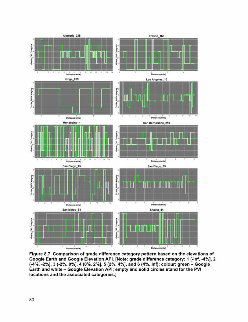
Figure 8.7. Comparison of grade difference category pattern based on the elevations ofGoogle Earth and Google Elevation API. [Note: grade difference category: 1 (-Inf, -4%], 2 (-4%, -2%], 3 (-2%, 0%], 4 (0%, 2%], 5 (2%, 4%], and 6 (4%, Inf); colour: green – Google Earth and white – Google Elevation API; empty and solid circles stand for the PVI locations and the associated categories.]
80
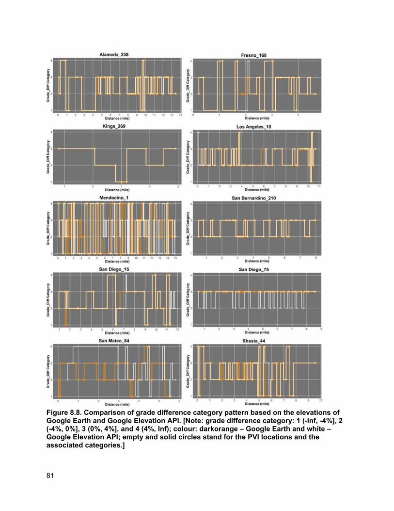
Figure 8.8. Comparison of grade difference category pattern based on the elevations ofGoogle Earth and Google Elevation API. [Note: grade difference category: 1 (-Inf, -4%], 2 (-4%, 0%], 3 (0%, 4%], and 4 (4%, Inf); colour: darkorange – Google Earth and white – Google Elevation API; empty and solid circles stand for the PVI locations and the associated categories.]
81
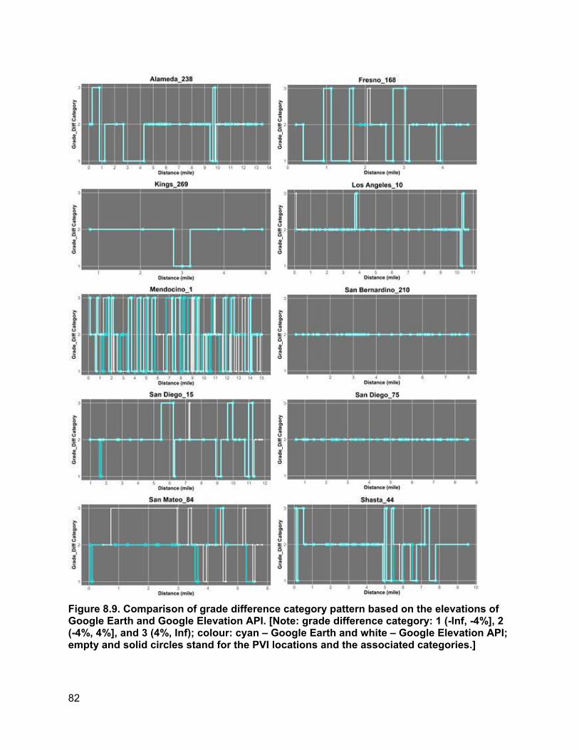
Figure 8.9. Comparison of grade difference category pattern based on the elevations of Google Earth and Google Elevation API. [Note: grade difference category: 1 (-Inf, -4%], 2 (-4%, 4%], and 3 (4%, Inf); colour: cyan – Google Earth and white – Google Elevation API;empty and solid circles stand for the PVI locations and the associated categories.]
82

Key findings from the grade difference pattern matching figures include the following: 1. Perfect pattern matching occurred on the route Kings_269 for all three category types.
“Perfect matching” means both patterns have the same number of PVI points and their PVI locations are very close. The Kings_269 route has relatively simple terrain compared with the other routes.
2. Generally speaking, when categories become more coarse, pattern matching is improved. Examples include Alameda_238, Los Angeles_10, San Bernardino_210, and San Diego_75.
3. From Figure 14 (the coarsest category type), the two most inconsistent patterns are Mendocino_1 and San Mateo_84.
8.4. PVI Identification Error and PVI Redistribution Error To further explore the category robustness of percent grade difference estimated from Google Elevation API and Google Earth, the following steps were followed:
• Step 1: within a TASAS segment, assign percent grade difference value to appropriate category
• Step 2: within a TASAS segment, count the number of percent grade difference values for each category.
• Step 3: conduct steps 1 and 2 for Google API and Google Earth respectively. • Step 4: determine the number difference (error) between Google API and Google Earth
(as shown in Figure 8.10).
Figure 8.10presents a schematic diagram that determines the number difference (or error) of the numbers of percent grade difference per category per segment between Google Elevation API and Google Earth, where 𝑁𝑁𝑠𝑠𝑖𝑖 ,𝐺𝐺𝐺𝐺 is the number of grade difference assigned to ith category and jth segment based on Google Elevation API; 𝑁𝑁𝑠𝑠𝑖𝑖 ,𝐺𝐺𝐺𝐺 is the number of grade difference assigned to ith category and jth segment based on Google Earth; and, 𝑒𝑒𝑠𝑠𝑖𝑖 = 𝑁𝑁𝑠𝑠𝑖𝑖 ,𝐺𝐺𝐺𝐺 − 𝑁𝑁𝑠𝑠𝑖𝑖 ,𝐺𝐺𝐺𝐺 .
Figure 8.10. Schematic diagram to define the number difference of the numbers of percent grade differences per category per segment between Google Elevation API and Google Earth
The error distribution charts for ten selected routes, Alameda_238, Fresno_168, Kings_269, Los Angeles_10, Mendocino_1, San Bernardino_210, San Diego_15, San Diego_75, San Mateo_84, and Shasta_44, are shown in Figures 16 through 25 respectively. Each chart
83

includes the error distributions of three category types, namely, Cat1 (-Inf, -4, -2, 0, 2, 4, Inf), Cat2 (-Inf, -4, 0, 4, Inf), and Cat3 (-Inf, -4, 4, Inf). For each category type, the errors were distributed over the domain constructed by category and TASAS segment. Notice that the grey- colored cells represent the cells with zero errors, i.e., 𝑒𝑒𝑖𝑖j = 0.
The following examples of the route Mendocino_1 (Figure 8.15) reveal two types of errors, PVI identification error and PVI redistribution error, which help to explain the category robustness study.
For Google API-based estimation, the consecutive percent grade difference values in the 12th
segment were -5.19, 6.16, -3.64, 1.62, -1.50, 1.50, -6.05, -4.22, 2.34, 2.80, -2.43, and -2.95 (a
total of 12 values). For Google Earth-based estimation, there are only three consecutive percent
grade difference values in the 12th segment as follows: -6.32, 4.15, and -7.12 (a total of 3
values). In other words, Google API identified 9 more PVI points than Google Earth. The
number 9 is coincidentally the same values of | ∑ 𝑖𝑖 𝑒𝑒 𝑖𝑖 j | = 9 for all three category types in the 12th
segment. The error | ∑ 𝑖𝑖 𝑒𝑒 𝑖𝑖 j | caused by more/fewer PVI points when comparing Google API-based or Google Earth-based estimations will be designated as PVI identification error.
In the 24th segment of route Mendocino_1, only one PVI point was identified by both Google
API-based and Google Earth-based estimation. The percent grade difference was -2.11 for
Google API and -1.47 for Google Earth. In this segment, there is no PVI identification error, i.e.,
| ∑ 𝑖𝑖 𝑒𝑒 𝑖𝑖 j | = 0. There are two errors occurred in the categories of (-4, -2] and (-2, 0] of Cat1 category; however, these errors were eliminated when adjusting the category definitions to Cat2
or Cat3. There errors occurred in Cat1 were named PVI redistribution error.
In the 19th segment of route Mendocino_1, Google API-based estimation identified 5 PVI points
with the consecutive percent grade difference values: -17.34, 18.50, -11.71, -6.10, and 3.10; 3
PVI points with the values of -2.98, 7.56, and -11.57 were identified by Google Earth-based
estimation. Viewing from Figure 20, it is immediately recognized that the PVI identification error
equals | ∑ 𝑖𝑖 𝑒𝑒𝑖𝑖 j | = 2 for all three category type. In addition to the PVI identification error, there two
errors occurred respectively in (-4, -2] and (2, 4] categories of Cat1 and two errors happened in
(-4, 0] and (0, 4] categories of Cat2. However, these errors were vanished in Cat3. Those two
errors occurred in Cat1 or Cat2 are PVI redistribution errors. The redistribution error can be
further defined as ∑ 𝑖𝑖 | 𝑒𝑒 𝑖𝑖 j | − | ∑ 𝑖𝑖 𝑒𝑒 𝑖𝑖 j |.
Another example of Los Angeles_10 was chosen to verify the definitions. In the third segment of
Los Angeles_10, only one PVI point was recognized by both Google API and Google Earth. The
84
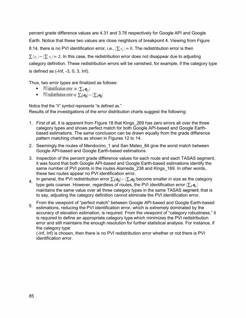
percent grade difference values are 4.31 and 3.76 respectively for Google API and Google
Earth. Notice that these two values are close neighbors of breakpoint 4. Viewing from Figure
8.14, there is no PVI identification error, i.e., | ∑𝑖𝑖 𝑒𝑒𝑖𝑖 j | = 0. The redistribution error is then
∑ 𝑖𝑖 | 𝑒𝑒 𝑖𝑖 j | − | ∑ 𝑖𝑖 𝑒𝑒𝑖𝑖 j | = 2. In this case, the redistribution error does not disappear due to adjusting category definition. These redistribution errors will be vanished, for example, if the category type
is defined as (-Inf, -3, 0, 3, Inf).
Thus, two error types are finalized as follows: • •
PVI identification error ≡ | ∑ 𝑖𝑖 𝑒𝑒 𝑖𝑖 j | PVI redistribution error ≡ ∑ 𝑖𝑖 | 𝑒𝑒 𝑖𝑖 j | − | ∑ 𝑖𝑖 𝑒𝑒 𝑖𝑖 j |
Notice that the “≡” symbol represents “is defined as.” Results of the investigations of the error distribution charts suggest the following:
1. First of all, it is apparent from Figure 18 that Kings_269 has zero errors all over the three category types and shows perfect match for both Google API-based and Google Earth- based estimations. The same conclusion can be drawn equally from the grade difference pattern matching charts as shown in Figures 12 to 14. Seemingly the routes of Mendocino_1 and San Mateo_84 give the worst match between Google API-based and Google Earth-based estimations. Inspection of the percent grade difference values for each route and each TASAS segment, it was found that both Google API-based and Google Earth-based estimations identify the same number of PVI points in the routes Alameda_238 and Kings_169. In other words, these two routes appear no PVI identification error. In general, the PVI redistribution error ∑ 𝑖𝑖 | 𝑒𝑒 𝑖𝑖 j | − | ∑ 𝑖𝑖 𝑒𝑒 𝑖𝑖 j | become smaller in size as the category type gets coarser. However, regardless of routes, the PVI identification error | ∑ 𝑖𝑖 𝑒𝑒 𝑖𝑖 j | maintains the same value over all three category types in the same TASAS segment; that is to say, adjusting the category definition cannot eliminate the PVI identification error. From the viewpoint of “perfect match” between Google API-based and Google Earth-based estimations, reducing the PVI identification error, which is extremely dominated by the accuracy of elevation estimation, is required. From the viewpoint of “category robustness,” it is required to define an appropriate category type which minimizes the PVI redistribution error and still maintains the enough resolution for further statistical analysis. For instance, if the category type (-Inf, Inf) is chosen, then there is no PVI redistribution error whether or not there is PVI identification error.
2.
3.
4.
5.
85
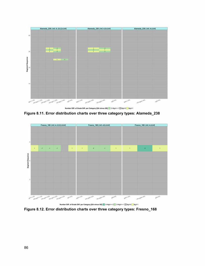
Figure 8.11. Error distribution charts over three category types: Alameda_238
Figure 8.12. Error distribution charts over three category types: Fresno_168
86

Figure 8.13. Error distribution charts over three category types: Kings_269
Figure 8.14. Error distribution charts over three category types: Los Angeles_10
87
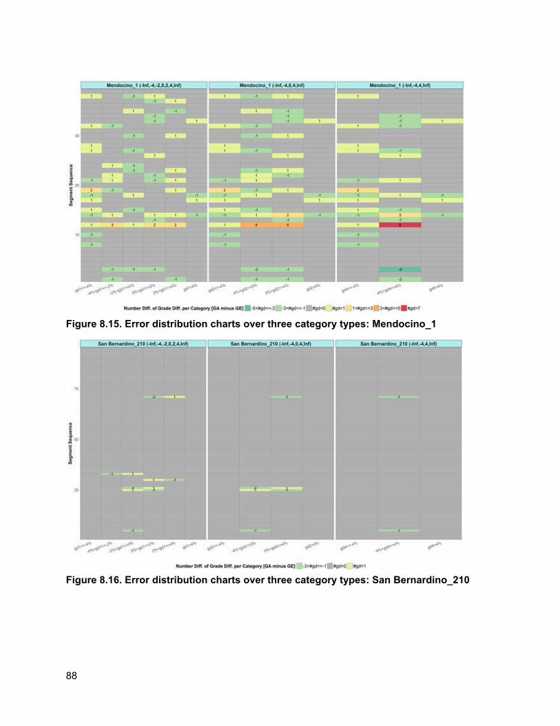
Figure 8.15. Error distribution charts over three category types: Mendocino_1
Figure 8.16. Error distribution charts over three category types: San Bernardino_210
88
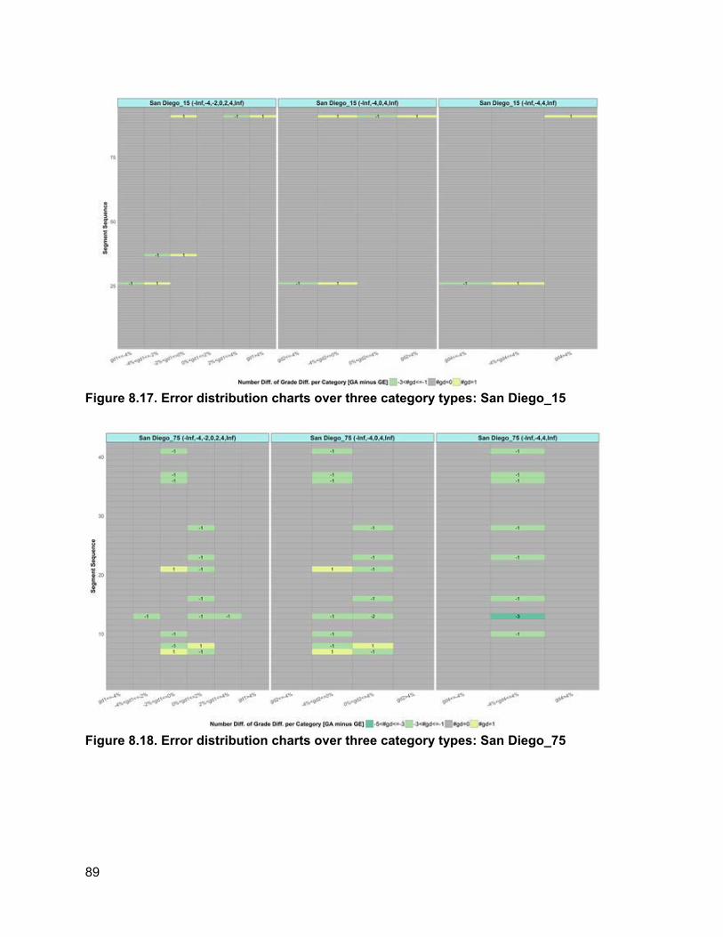
Figure 8.17. Error distribution charts over three category types: San Diego_15
Figure 8.18. Error distribution charts over three category types: San Diego_75
89
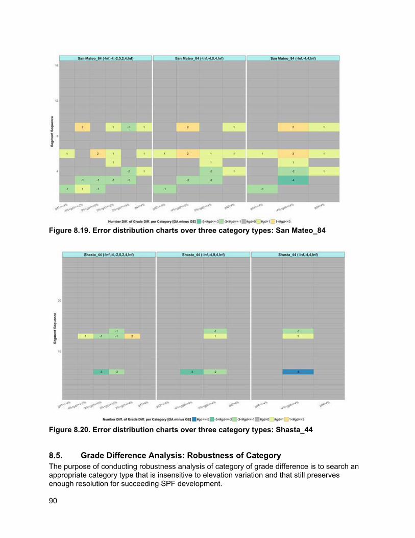
Figure 8.19. Error distribution charts over three category types: San Mateo_84
Figure 8.20. Error distribution charts over three category types: Shasta_44
8.5. Grade Difference Analysis: Robustness of Category The purpose of conducting robustness analysis of category of grade difference is to search an appropriate category type that is insensitive to elevation variation and that still preserves enough resolution for succeeding SPF development.
90
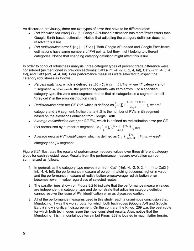
As discussed previously, there are two types of error that have to be differentiated: • PVI identification error | Σ𝑖𝑖 𝑒𝑒 𝑖𝑖j | Google API-based estimation has more/fewer errors than
Google Earth-based estimation. Notice that adjusting the category definition does not resolve this issue. PVI redistribution error Σ𝑖𝑖 |𝑒𝑒 𝑖𝑖j | − | Σ𝑖𝑖 𝑒𝑒 𝑖𝑖j | Both Google API-based and Google Earth-based estimations have same numbers of PVI points, but they might belong to different categories. Notice that changing category definition might affect this issue.
•
In order to conduct robustness analysis, three category types of percent grade difference were considered (as mentioned in previous sections): Cat1 (-Inf, -4, -2, 0, 2, 4, Inf), Cat2 (-Inf, -4, 0, 4, Inf), and Cat3 (-Inf, -4, 4, Inf). Four performance measures were selected to inspect the category robustness as follows:
• Percent matching, which is defined as 100 × ∑j #( ∀i 𝑒𝑒 𝑖𝑖 j = 0 )⁄#seg , where i ≡ category and j ≡ segment; in other words, the percent segments with zero errors. For a specified category type, the zero-error segment means that all categories in a segment are all “grey cells” in the error distribution chart.
1 • Redistribution error per GE PVI, which is defined as × ), wherei
∑ j ( 2 #𝑝𝑝vi ⱼ , GE
category and j ≡ segment. Notice that # 𝑝𝑝vi ⱼ , GE is the number of PVIs in jth segment based on the elevations obtained from Google Earth. Average redistribution error per GE PVI, which is defined as redistribution error per GE •
Σ𝑖𝑖 |𝑒𝑒𝑖𝑖 j| − | Σ𝑖𝑖 𝑒𝑒 𝑖𝑖j
1 PVI normalized by number of segment, i.e., × ∑ ( 2 j ) / #𝑠𝑠eg.
# 𝑝𝑝vi ⱼ , GE
Average error in PVI identification, which is defined as ∑ ( | ∑ i 𝑒𝑒 ij | ) #𝑠𝑠𝑠𝑠𝑒𝑒𝑒𝑒𝑠𝑠𝑠𝑠, where i ≡ • j #pvi ⱼ, GE
category and j ≡ segment.
Figure 8.21 illustrates the results of performance measure values over three different category types for each selected route. Results from the performance measure evaluation can be summarized as follows:
1. In general, as the category type moves fromfrom Cat1 (-Inf, -4, -2, 0, 2, 4, Inf) to Cat3 (- Inf, -4, 4, Inf), the performance measure of percent matching becomes higher in value and the performance measure of redistribution error/average redistribution error becomes lower in value regardless of selected routes. The parallel lines shown on Figure 8.21d indicate that the performance measure values are independent in category type and demonstrate that adjusting category definition cannot resolve the issue of PVI identification error as discussed earlier. All of the performance measures used in this study reach a unanimous conclusion that Mendocino_1 was the worst route, for which both techniques (Google API and Google Earth) show significant disagreement. On the contrary, the Kings_269 was the best route for which both techniques issue the most consistent results. Also, notice that the Mendocino_1 is in mountainous terrain but Kings_269 is located in much flatter terrain.
2.
3.
91
Σ𝑖𝑖 |𝑒𝑒𝑖𝑖j | − | Σ𝑖𝑖 𝑒𝑒 𝑖𝑖j |
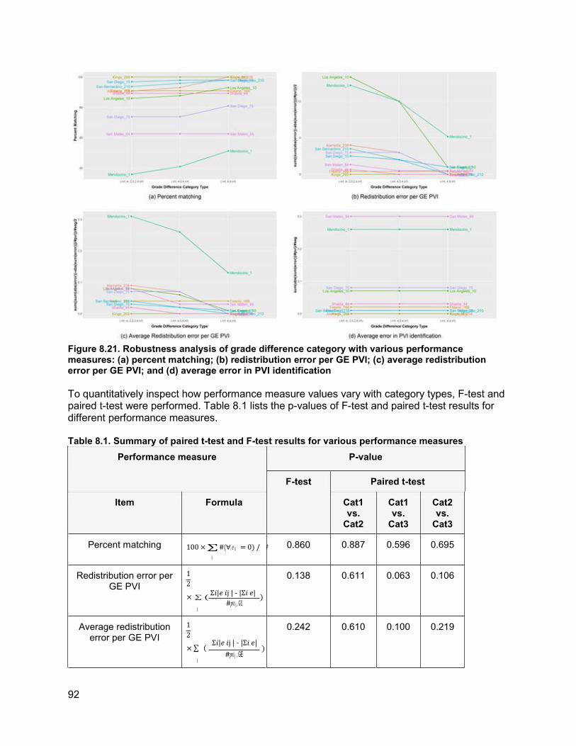
Figure 8.21. Robustness analysis of grade difference category with various performance measures: (a) percent matching; (b) redistribution error per GE PVI; (c) average redistribution error per GE PVI; and (d) average error in PVI identification
To quantitatively inspect how performance measure values vary with category types, F-test and paired t-test were performed. Table 8.1 lists the p-values of F-test and paired t-test results for different performance measures.
Table 8.1. Summary of paired t-test and F-test results for various performance measures
92
Performance measure
P-value
F-test
Paired t-test
Item
Formula
Cat1 vs.
Cat2
Cat1 vs.
Cat3
Cat2 vs.
Cat3
Percent matching
100 × ∑ #(∀i 𝑒𝑒 i j = 0) /
j
# 0.860
0.887
0.596
0.695
Redistribution error per GE PVI
1 2
× ∑ ( )
#𝑝𝑝vi ⱼ , GE j
0.138
0.611
0.063
0.106
Average redistribution error per GE PVI
1 2
Σ𝑖𝑖|𝑒𝑒 𝑖𝑖j | - |Σ𝑖𝑖 𝑒𝑒| × ∑ ( )
#𝑝𝑝vi ⱼ , GE j
0.242
0.610
0.100
0.219
Σ𝑖𝑖|𝑒𝑒 𝑖𝑖j | - |Σ𝑖𝑖 𝑒𝑒| 𝑖𝑖j|
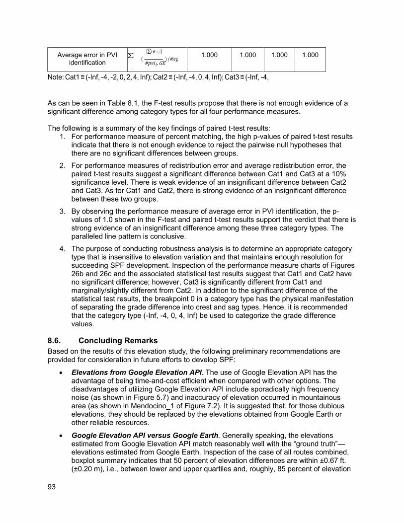
Note: Cat1 ≡ (-Inf, -4, -2, 0, 2, 4, Inf); Cat2 ≡ (-Inf, -4, 0, 4, Inf); Cat3 ≡ (-Inf, -4,
As can be seen in Table 8.1, the F-test results propose that there is not enough evidence of a significant difference among category types for all four performance measures.
The following is a summary of the key findings of paired t-test results: 1. For performance measure of percent matching, the high p-values of paired t-test results
indicate that there is not enough evidence to reject the pairwise null hypotheses that there are no significant differences between groups. For performance measures of redistribution error and average redistribution error, the paired t-test results suggest a significant difference between Cat1 and Cat3 at a 10% significance level. There is weak evidence of an insignificant difference between Cat2 and Cat3. As for Cat1 and Cat2, there is strong evidence of an insignificant difference between these two groups. By observing the performance measure of average error in PVI identification, the p- values of 1.0 shown in the F-test and paired t-test results support the verdict that there is strong evidence of an insignificant difference among these three category types. The paralleled line pattern is conclusive. The purpose of conducting robustness analysis is to determine an appropriate category type that is insensitive to elevation variation and that maintains enough resolution for succeeding SPF development. Inspection of the performance measure charts of Figures 26b and 26c and the associated statistical test results suggest that Cat1 and Cat2 have no significant difference; however, Cat3 is significantly different from Cat1 and marginally/slightly different from Cat2. In addition to the significant difference of the statistical test results, the breakpoint 0 in a category type has the physical manifestation of separating the grade difference into crest and sag types. Hence, it is recommended that the category type (-Inf, -4, 0, 4, Inf) be used to categorize the grade difference values.
2.
3.
4.
8.6. Concluding Remarks Based on the results of this elevation study, the following preliminary recommendations are provided for consideration in future efforts to develop SPF:
• Elevations from Google Elevation API. The use of Google Elevation API has the advantage of being time-and-cost efficient when compared with other options. The disadvantages of utilizing Google Elevation API include sporadically high frequency noise (as shown in Figure 5.7) and inaccuracy of elevation occurred in mountainous area (as shown in Mendocino_1 of Figure 7.2). It is suggested that, for those dubious elevations, they should be replaced by the elevations obtained from Google Earth or other reliable resources.
Google Elevation API versus Google Earth. Generally speaking, the elevations estimated from Google Elevation API match reasonably well with the “ground truth”— elevations estimated from Google Earth. Inspection of the case of all routes combined, boxplot summary indicates that 50 percent of elevation differences are within ±0.67 ft. (±0.20 m), i.e., between lower and upper quartiles and, roughly, 85 percent of elevation
•
93
Average error in PVI identification
| ∑ⅰ 𝑒𝑒 ⅰ ⱼ | ∑
( ) /#𝑠𝑠eg #pvi ⱼ, GE
j
1.000
1.000
1.000
1.000

differences (non-outliers) are within ±2.67 ft. (±0.81 m), i.e., between l15iqr and r15iqr (please refer to Figure 3 for definitions).
Algorithm that determines PVI points. In this study, piecewise regression was utilized to determine grades, PVI locations, and grade differences at PVI points. It was found that the piecewise regression results were affected not only by elevation noise but also by station interval. The simulation of slope variation at fixed position under various elevation noises indicates that position near sag/crest of a vertical alignment appears to be less stable (highly varied). As seen in the simulation example of Figure 8.5, when apply the same piecewise regression algorithm, the number of PVI points really depends on the station interval. Further study is required to determine the appropriate station interval of vertical highway alignment to prevent oversampling (station intervals are too close) or undersampling (station intervals are too far) issue as noted in the simulation example.
Potential elevation variables for SPF development. To assign the vertical alignment features to TASAS segment, grade and grade difference, and number of PVI points were major candidates considered to develop SPF. Since the TASAS segment could be very long or very short, a segment might contain several different grades/PVI points or contain no PVI point at all. It is recommended to convert these numeric variables into category variables for SPF development.
Robustness analysis of grade difference category. Two types of error have been identified in the study of robustness analysis of category. One is 𝑃𝑃VI identification error ≡ | ∑ⅰ 𝑒𝑒 ⅰ j | ; the other is 𝑃𝑃VI redistribution error ≡ |∑ⅰ 𝑒𝑒𝑖𝑖 ⱼ | − | ∑ⅰ 𝑒𝑒 ⅰ j | . Adjusting category definition cannot eliminate the PVI identification error but can alter the PVI redistribution error. The purpose of conducting robustness analysis is to determine an appropriate category type that is insensitive to elevation variation and that maintains enough resolution for succeeding SPF development. Four performance measures, percent matching, redistribution error, average redistribution error, and average error in PVI identification, were applied to 10 selected routes for all three category types. Statistical results of F-test and paired t-test were utilized to inspect whether there are significant differences among category types. With the performance measure of redistribution error, hypothesis testing results indicate that there is no significant difference between Cat1 and Cat2; however, at 10% significance level, there is significant difference between Cat1 and Cat3 and between Cat2 and Cat3. In addition to hypothesis testing results, two factors were considered in selecting appropriate category type: (1) the breakpoint 0 in a category type has the physical meaning that can separate the grade difference into crest or sag; (2) almost 80% of grade difference values are within the range of (-4, 4). When considering all these aspects, it is recommended that the category type (-Inf, -4, 0, 4, Inf) be used to categorize the grade difference values for SPF development.
Potential elevation resources. A Caltrans project recently contracted by Pathway provides the vertical alignment features for entire California highway network. Those features include length of curve (L), locations (i.e., postmiles and latitudes/longitudes) of B.V.C (beginning of vertical curve) and E.V.C (end of vertical curve), distance in feet required to achieve a 1% change in grade (K), and beginning and end percent grades (G and G′). Based on this information, the grade difference and PVI location can be easily calculated and thus integrated into the TASAS database for the use of developing SPF. Unfortunately, the database conducted by Pathway is not available at the time of writing this report. Another potential elevation resource is the Elevation Automated Pavement
•
•
•
•
94

Condition Survey (APCS) database of Caltrans GIS library. The applicability of the APCS database requires further investigation.
95
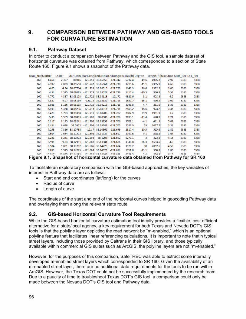
9. COMPARISON BETWEEN PATHWAY AND GIS-BASED TOOLS FOR CURVATURE ESTIMATION
9.1. Pathway Dataset In order to conduct a comparison between Pathway and the GIS tool, a sample dataset of horizontal curvature was obtained from Pathway, which corresponded to a section of State Route 160. Figure 9.1 shows a snapshot of the Pathway data.
Figure 9.1. Snapshot of horizontal curvature data obtained from Pathway for SR 160
To facilitate an exploratory comparison with the GIS-based approaches, the key variables of interest in Pathway data are as follows:
• Start and end coordinates (lat/long) for the curves • Radius of curve • Length of curve
The coordinates of the start and end of the horizontal curves helped in geocoding Pathway data and overlaying them along the relevant state route.
9.2. GIS-based Horizontal Curvature Tool Requirements While the GIS-based horizontal curvature estimation tool ideally provides a flexible, cost efficient alternative for a state/local agency, a key requirement for both Texas and Nevada DOT’s GIS tools is that the polyline layer depicting the road network be “m-enabled,” which is an optional polyline feature that facilitates linear referencing calculations. It is important to note thatin typical street layers, including those provided by Caltrans in their GIS library, and those typically available within commercial GIS suites such as ArcGIS, the polyline layers are not “m-enabled.”
However, for the purposes of this comparison, SafeTREC was able to extract some internally developed m-enabled street layers which corresponded to SR 160. Given the availability of an m-enabled street layer, there are no additional data requirements for the tools to be run within ArcGIS. However, the Texas DOT could not be successfully implemented by the research team. Due to a paucity of time to troubleshoot Texas DOT’s GIS tool, a comparison could only be made between the Nevada DOT’s GIS tool and Pathway data.
96
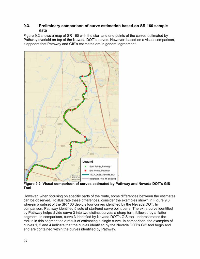
9.3. Preliminary comparison of curve estimation based on SR 160 sample data
Figure 9.2 shows a map of SR 160 with the start and end points of the curves estimated by Pathway overlaid on top of the Nevada DOT’s curves. However, based on a visual comparison, it appears that Pathway and GIS’s estimates are in general agreement.
Figure 9.2. Visual comparison of curves estimated by Pathway and Nevada DOT’s GIS Tool
However, when focusing on specific parts of the route, some differences between the estimates can be observed. To illustrate these differences, consider the examples shown in Figure 9.3 wherein a subset of the SR 160 depicts four curves identified by the Nevada DOT. In comparison, Pathway identified 5 sets of start/end curve point pairs. The extra curve identified by Pathway helps divide curve 3 into two distinct curves: a sharp turn, followed by a flatter segment. In comparison, curve 3 identified by Nevada DOT’s GIS tool underestimates the radius in this segment as a result of estimating a single curve. In comparison, the examples of curves 1, 2 and 4 indicate that the curves identified by the Nevada DOT’s GIS tool begin and end are contained within the curves identified by Pathway.
97
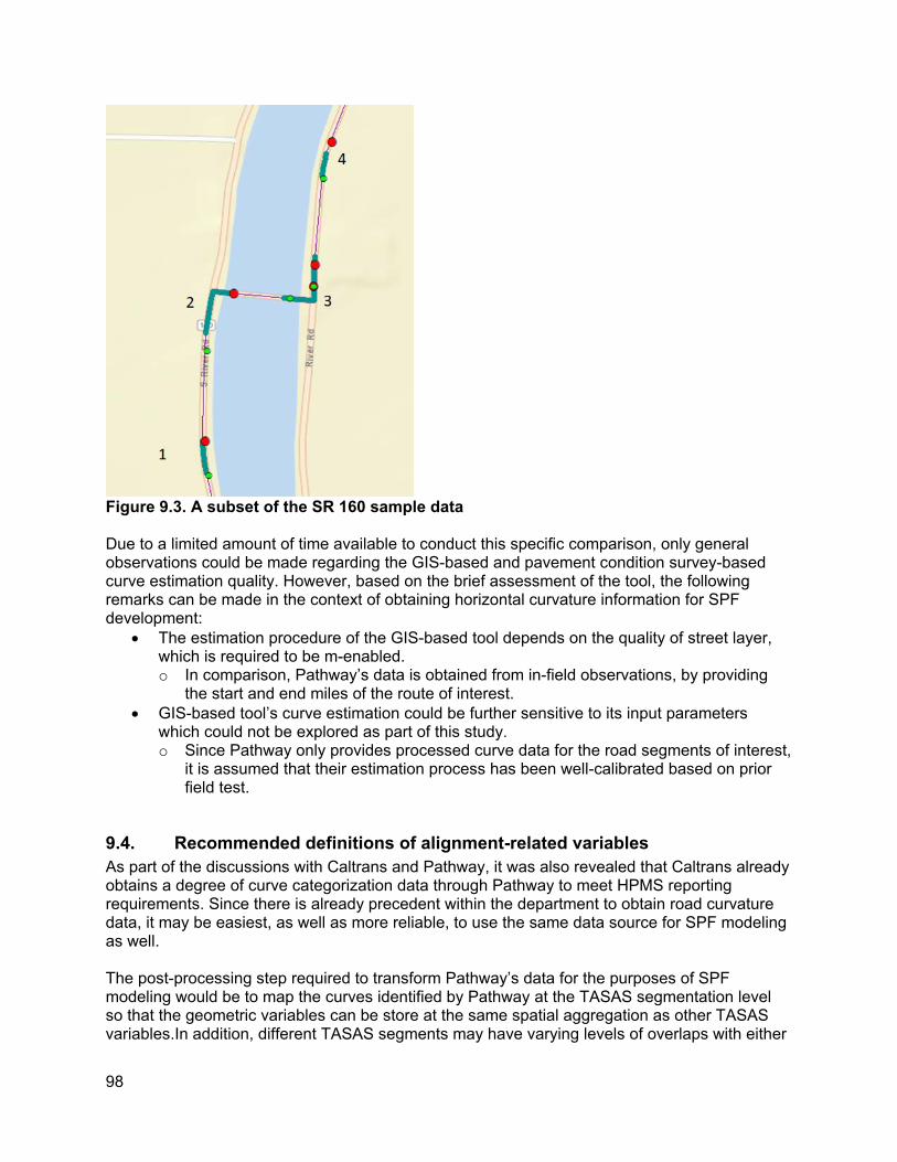
Figure 9.3. A subset of the SR 160 sample data
Due to a limited amount of time available to conduct this specific comparison, only general observations could be made regarding the GIS-based and pavement condition survey-based curve estimation quality. However, based on the brief assessment of the tool, the following remarks can be made in the context of obtaining horizontal curvature information for SPF development:
• The estimation procedure of the GIS-based tool depends on the quality of street layer, which is required to be m-enabled. o In comparison, Pathway’s data is obtained from in-field observations, by providing
the start and end miles of the route of interest. • GIS-based tool’s curve estimation could be further sensitive to its input parameters
which could not be explored as part of this study. o Since Pathway only provides processed curve data for the road segments of interest,
it is assumed that their estimation process has been well-calibrated based on prior field test.
9.4. Recommended definitions of alignment-related variables As part of the discussions with Caltrans and Pathway, it was also revealed that Caltrans already obtains a degree of curve categorization data through Pathway to meet HPMS reporting requirements. Since there is already precedent within the department to obtain road curvature data, it may be easiest, as well as more reliable, to use the same data source for SPF modeling as well.
The post-processing step required to transform Pathway’s data for the purposes of SPF modeling would be to map the curves identified by Pathway at the TASAS segmentation level so that the geometric variables can be store at the same spatial aggregation as other TASAS variables.In addition, different TASAS segments may have varying levels of overlaps with either
98
zero, one or multiple horizontal and vertical curves. To accommodate these different considerations, the alignment-related variables shall be defined as ordinal categories (similar to HPMS reporting requirements).
The following are the alignment-related variables that are recommended for SPF consideration, and which can be populated within TASAS for each segment: 1. Horizontal alignment:
a. Degree of curvature categories (as defined under HPMS requirements): Category Degree of Curvature
Range A <3.5 B 3.5 – 5.4 C 5.5 – 8.4 D 8.5 – 13.9 E 14.0 – 27.9 F > 28.0
Note: degree of curvature would have to be calculated by Pathway as discussed in section 4.2.3.1. It can also be potentially estimated for cross-street approaches using GIS tools.
b. Central angle (which is currently defined as the variable “degree” in Pathway’s data): Category Central Angle
Range A <30 B 30 –59.9 C 60 – 89.9 D 90 – 119.9 E >120
Note: central angle is readily available for mainline segments using Pathway, but may not be readily available in the GIS-based HPMS reporting tools
2. Vertical alignment: a. Grade difference (based on the robust analysis assessmentin chapter 8):
Category Grade Difference Range
A <-4% B -4%– -0.1% C 0%–4% D > 4%
Note: Grade difference for each curve in Pathway data would also have to be calculated as the difference initial and final grade, both of which are available in their database. It can also be estimated for cross-street approaches using Google’s elevation API, as discussed in section 5.3 and chapter 8.
b. Rate of vertical curvature (K-value): Design guidelines recommend different K values for a range of different design speeds. Using those guidelines as input, the following K categories have been recommended:
99

Category K-value Range
Associated Design Speed Range
A <100 < 50 B 100 –149.9 50 – 59 C 150 –249.9 60 – 79 D >250 > 70
Note: The design speeds provided above are shown only for reference purposes to indicate how the K-value ranges were determined, and should not be interpreted as categories for design speeds themselves. This variable is not available for the cross-street approaches.
In order to populate these categorical variables for each segment, the total length (or the percentage) of a segment corresponding to each category can be estimated and entered. For instance, if a segment of length 1 mile has four horizontal curves as follows:
• One curve of 0.3 miles with degree of curvature type A • Two curves of 0.2 miles with degree of curvature type C • One curve of 0.3 miles with degree of curvature type E
Using this information, the variables corresponding to the six degree of curvature categories (A through F) would have the following values:
Degree of Curvature Categories (Example)
A B C D E F 0.3 0 0.4 0 0.3 0
100

10. CONCLUSION AND RECOMMENDATIONS
10.1. Summary of results
Table 10.1 provides an overview of the suitability analysis for the different data sources based on the findings from Chapters 4, 7, and 9.
Table 10.1. Summary of the suitability analysis
Data Source Variable Completeness Frequency of Updates
Spatial Variation
Data Sources Within Caltrans
TASAS Segments AADT Yes Yes1 Yes2
Non-AADT Yes Insufficient Information2
Insufficient Information2
TASAS Intersections
Mainline AADT Yes Yes1 N/A Cross-street AADT Yes No N/A
Non-AADT Yes Insufficient Information2 N/A
TASAS Ramps AADT Yes No1 Yes
Non-AADT Yes Insufficient Information2 N/A
Traffic Census Truck Volumes No No1 No
Pathway Horizontal Alignment Yes Yes Yes
Vertical Alignment Yes Yes Yes
Photolog Horizontal Alignment No No No
Vertical Alignment No No No
Data Sources Outside of Caltrans
Google Earth/Google Street View
Clear Zone Yes Insufficient Information3 Yes
Driveway Yes Insufficient Information3 Yes
Central Left Turn Lane Yes Insufficient Information3 Yes
Crosswalk Presence/Type Yes Insufficient Information3 N/A
Speed Limits Yes Insufficient Information3 Yes
101
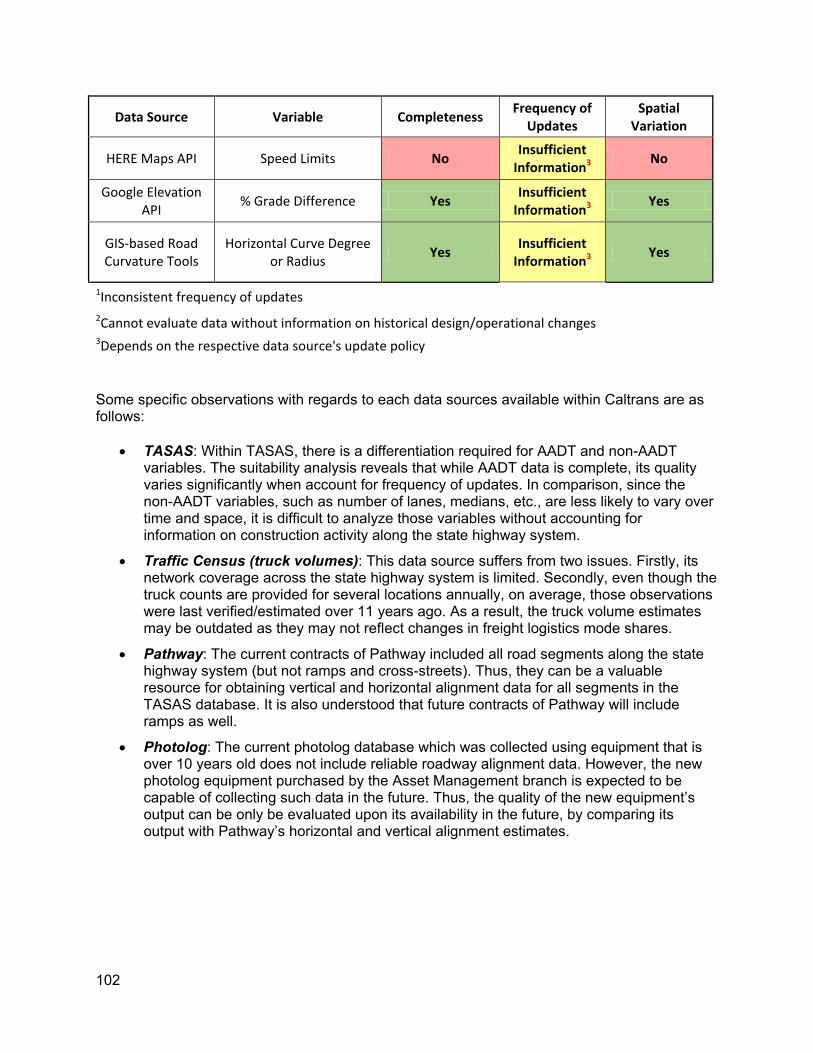
Data Source Variable Completeness Frequency of Updates
Spatial Variation
HERE Maps API Speed Limits No Insufficient Information3 No
Google Elevation API % Grade Difference Yes Insufficient
Information3 Yes
GIS-based Road Curvature Tools
Horizontal Curve Degree or Radius Yes Insufficient
Information3 Yes
1Inconsistent frequency of updates 2Cannot evaluate data without information on historical design/operational changes 3Depends on the respective data source's update policy
Some specific observations with regards to each data sources available within Caltrans are as follows:
• TASAS: Within TASAS, there is a differentiation required for AADT and non-AADT variables. The suitability analysis reveals that while AADT data is complete, its quality varies significantly when account for frequency of updates. In comparison, since the non-AADT variables, such as number of lanes, medians, etc., are less likely to vary over time and space, it is difficult to analyze those variables without accounting for information on construction activity along the state highway system.
• Traffic Census (truck volumes): This data source suffers from two issues. Firstly, its network coverage across the state highway system is limited. Secondly, even though the truck counts are provided for several locations annually, on average, those observations were last verified/estimated over 11 years ago. As a result, the truck volume estimates may be outdated as they may not reflect changes in freight logistics mode shares.
• Pathway: The current contracts of Pathway included all road segments along the state highway system (but not ramps and cross-streets). Thus, they can be a valuable resource for obtaining vertical and horizontal alignment data for all segments in the TASAS database. It is also understood that future contracts of Pathway will include ramps as well.
• Photolog: The current photolog database which was collected using equipment that is over 10 years old does not include reliable roadway alignment data. However, the new photolog equipment purchased by the Asset Management branch is expected to be capable of collecting such data in the future. Thus, the quality of the new equipment’s output can be only be evaluated upon its availability in the future, by comparing its output with Pathway’s horizontal and vertical alignment estimates.
102

Some specific observations with regards to data source available outside of Caltrans are as follows:
• Google Earth/Google Street View: The combination of aerial imagery and street view data provided by Google provides a flexible approach to collect variables manually through visual inspection. This approach is particularly helpful to systematically populate previously unavailable variables which may be hard to reliably estimate through commercially available databases such as clear zone width, driveway counts. However, since it is a time consuming effort, the data collection requires the development of robust protocols to ensure that the data are collected in a standardized manner.
• HERE Maps API: This API was utilized to collect posted speed limit information as part of the pilot project. Based on the findings of the pilot study, it was found that using the highest resolution of the speed limit API did not always provide an estimate in the vicinity of the location being queried. In addition, local variations in the speed limit, such as near schools and along curves, were also not captured by it. However, it presents a scalable approach to obtain speed limits across the state highway system.
• Google Elevation API: Google Elevation API provides an alternate methodology to estimate the vertical alignment profile and identify sag/crest curves using elevation data obtained from satellite imagery.Based on the findings of the pilot study, it is observed that while the estimated profile is largely consistent with ground truth observed from Google StreetView, substantial deviations were observed in some locations perhaps due to uneven terrains, etc.
• GIS-based road curvature tools: The GIS tools obtained from Texas DOT and Nevada DOT provide an alternate data source to estimate radius/degree of curvature using GIS street layers. There are two specific concerns with this data source. Firstly, they require specific types of shapefiles which have linear referencing attributes, which aren’t readily available in commercial GIS software. Secondly, these tools require calibration of input parameters which impacts the quality of the estimated curves.
10.2. Recommendation for new and existing variables for SPF modeling
Based on the insights gained from the suitability analysis, some recommendations for the suitability of the data elements discussed in this study for SPF estimation can be made. Table 10.2 and 10.3 provide the recommendations organized by data sources and variables respectively. In addition to the determination of whether the variable is suitable given the constraints of the SPF data needs requirements, the tables also provide quality control measures which can be applied to future data to assess whether the inputs to the SPF modeling are consistently improving. Finally, the recommendations provided for each variable include policy recommendations to ensure periodic traffic volume updates, as well as programmatic coordination activities to maximize data availability in the future.
103
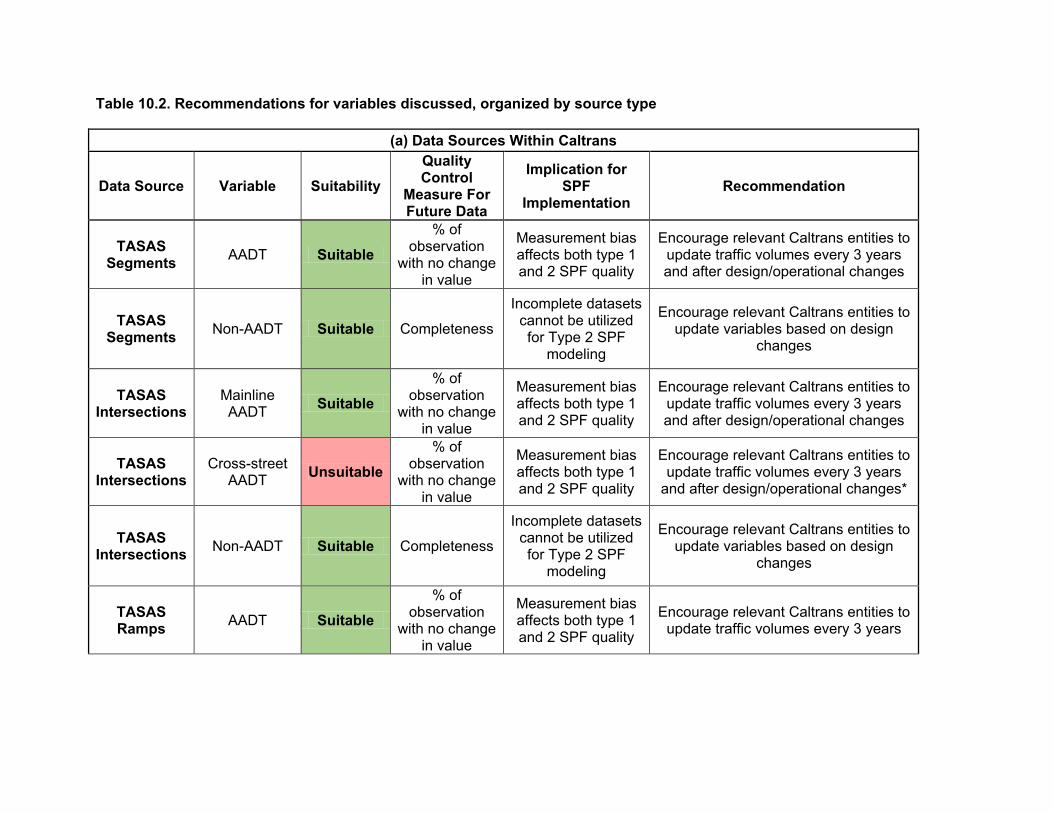
Table 10.2. Recommendations for variables discussed, organized by source type
(a) Data Sources Within Caltrans Quality Implication for Control Data Source Variable Suitability SPF Recommendation Measure For Implementation Future Data
% of Measurement bias Encourage relevant Caltrans entities to TASAS observation AADT Suitable affects both type 1 update traffic volumes every 3 years with no change Segments and 2 SPF quality and after design/operational changes in value Incomplete datasets Encourage relevant Caltrans entities to TASAS cannot be utilized Non-AADT Suitable Completeness update variables based on design Segments for Type 2 SPF changes modeling
% of Measurement bias Encourage relevant Caltrans entities to TASAS Mainline observation affects both type 1 update traffic volumes every 3 years Suitable AADT with no change Intersections and 2 SPF quality and after design/operational changes in value % of Measurement bias Encourage relevant Caltrans entities to observation TASAS Cross-street Unsuitable affects both type 1 update traffic volumes every 3 years Intersections AADT with no change and 2 SPF quality and after design/operational changes* in value
Incomplete datasets Encourage relevant Caltrans entities to cannot be utilized TASAS Non-AADT Suitable Completeness update variables based on design Intersections for Type 2 SPF changes modeling % of Measurement bias observation Encourage relevant Caltrans entities to TASAS AADT Suitable affects both type 1 update traffic volumes every 3 years Ramps with no change and 2 SPF quality in value
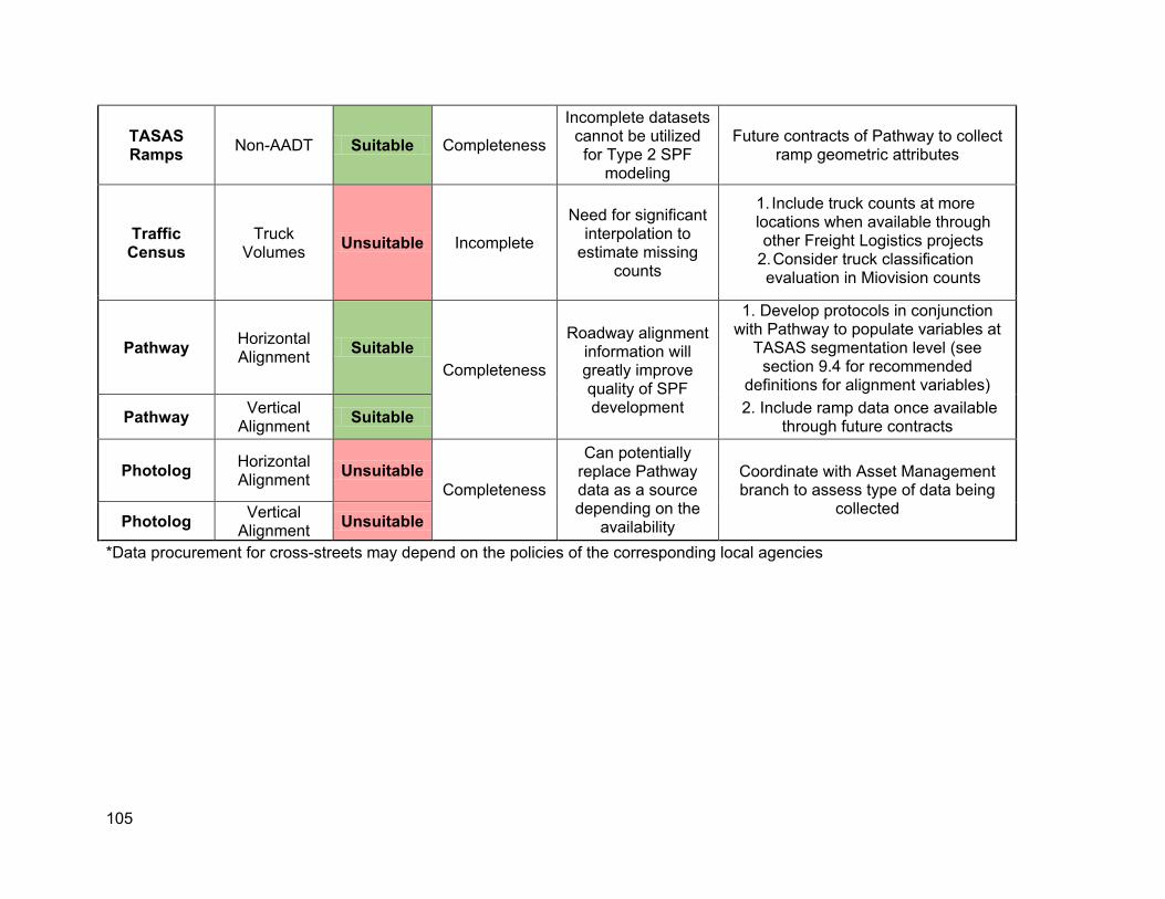
TASAS Ramps Non-AADT Suitable Completeness
Incomplete datasets cannot be utilized for Type 2 SPF
modeling
Future contracts of Pathway to collect ramp geometric attributes
Traffic Census
Truck Volumes Incomplete
Need for significant interpolation to
estimate missing counts
1. Include truck counts at more locations when available through other Freight Logistics projects
2.Consider truck classification evaluation in Miovision counts
Unsuitable
Pathway Horizontal Alignment Suitable
Completeness
Roadway alignment information will greatly improve quality of SPF development
1. Develop protocols in conjunction with Pathway to populate variables at
TASAS segmentation level (see section 9.4 for recommended
definitions for alignment variables) 2. Include ramp data once available
through future contracts Pathway
Photolog
Vertical Alignment
Horizontal Alignment
Suitable
Completeness
Can potentially replace Pathway data as a source depending on the
availability
Coordinate with Asset Management branch to assess type of data being
collected
Unsuitable
Photolog Vertical Alignment Unsuitable
*Data procurement for cross-streets may depend on the policies of the corresponding local agencies
105
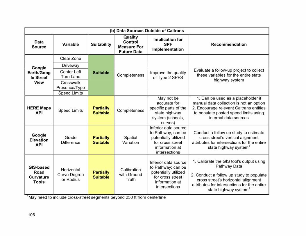
(b) Data Sources Outside of Caltrans
Data Source Variable Suitability
QualityControl
Measure For Future Data
Implication forSPF
Implementation Recommendation
Google Earth/Goog
le Street View
Clear Zone
Completeness Improve the quality of Type 2 SPFS
Evaluate a follow-up project to collect these variables for the entire state
highway system
Driveway Center Left Turn Lane
Suitable
Crosswalk Presence/Type Speed Limits
HERE MapsAPI Speed Limits Partially
Suitable Completeness
May not be accurate for
specific parts of the state highway
system (schools, curves)
1. Can be used as a placeholder if manual data collection is not an option 2. Encourage relevant Caltrans entities to populate posted speed limits using
internal data sources
Google Elevation
API Grade
Difference PartiallySuitable
Spatial Variation
Inferior data source to Pathway; can be potentially utilized
for cross street information at intersections
Conduct a follow up study to estimate cross street's vertical alignment
attributes for intersections for the entire state highway system1
GIS-based Road
Curvature Tools
Horizontal Curve Degree
or Radius
PartiallySuitable
Calibration with Ground
Truth
Inferior data source to Pathway; can be potentially utilized
for cross street information at intersections
1. Calibrate the GIS tool's output using Pathway Data
2. Conduct a follow up study to populate cross street's horizontal alignment
attributes for intersections for the entire state highway system1
1May need to include cross-street segments beyond 250 ft from centerline
106

Table 10.3 presents the recommendation organized by different variables that were analyzed through this project. In some instances, where multiple data sources may be potentially available, such as posted speed limits and horizontal and vertical alignment, specific sources have been prioritized over others based on the quality of data that can be obtained. For instance, based on the pilot study, it is observed that the HERE Maps API may not have sufficient spatial resolution to capture local variations in speed limits around curves and schools. Thus, it is recommended that posted speed limits be collected through visual inspection manually over the API as the primary data source for speed limits. Similarly, since Pathway provides a single source for horizontal and vertical alignment information for the mainline segments, it is recommended over GIS-based tools and Google Elevation API, which can be potentially utilized for locations where Pathway data is unlikely to collect any data (e.g., cross street segments).
In addition, Table 10.3 also categorizes the variables deemed suitable for SPF modeling into three categories:
• Existing variables (e.g., TASAS data) • New Variables:
o Need for data collection (e.g., clearzone) o Need for customization: Alignment data from Pathway
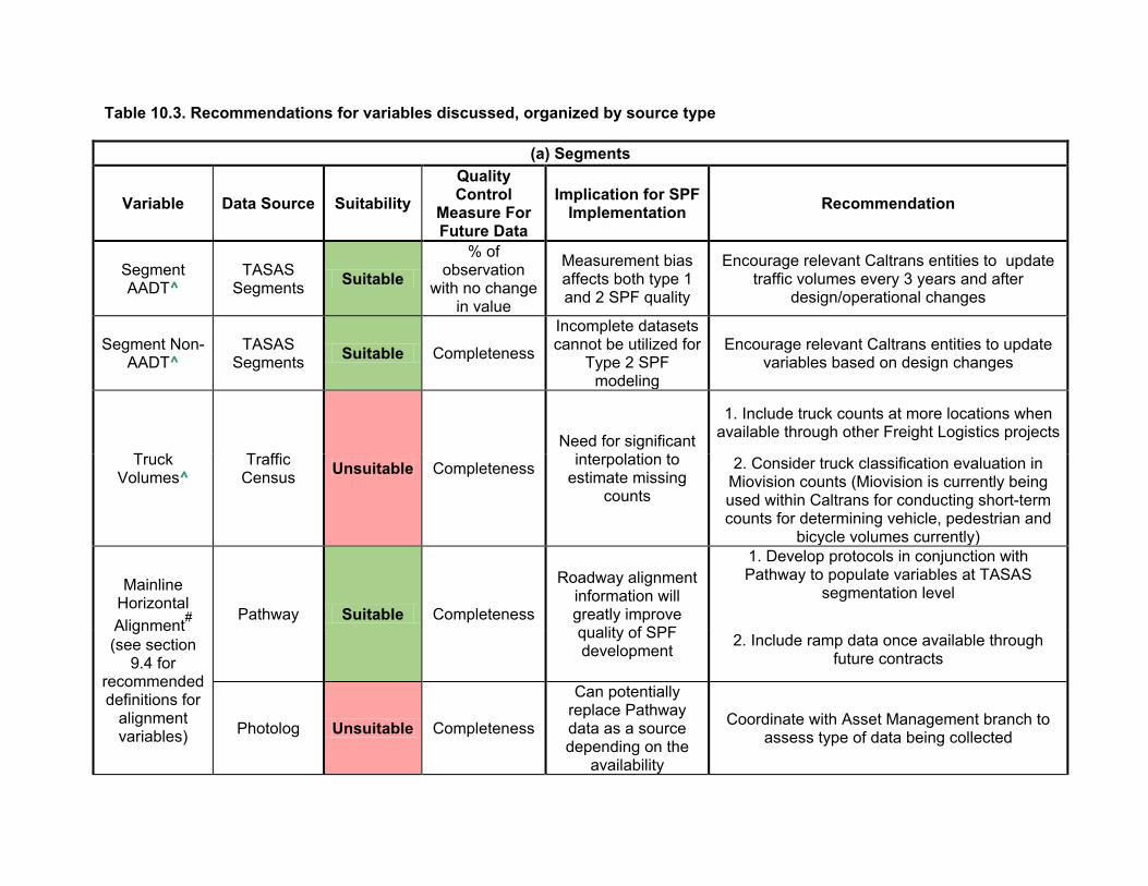
Table 10.3. Recommendations for variables discussed, organized by source type
(a) Segments Quality
Variable Data Source Suitability Control Measure For Future Data
Implication for SPF Implementation Recommendation
Segment AADT^
TASAS Segments Suitable
% of observation
with no change in value
Measurement bias affects both type 1 and 2 SPF quality
Encourage relevant Caltrans entities to update traffic volumes every 3 years and after
design/operational changes
Segment Non-AADT^
TASAS Segments Suitable Completeness
Incomplete datasets cannot be utilized for
Type 2 SPF modeling
Encourage relevant Caltrans entities to update variables based on design changes
1. Include truck counts at more locations when
Truck Volumes^
Traffic Census Unsuitable Completeness
Need for significant interpolation to
estimate missing counts
available through other Freight Logistics projects
2. Consider truck classification evaluation in Miovision counts (Miovision is currently being used within Caltrans for conducting short-term counts for determining vehicle, pedestrian and
bicycle volumes currently)
Mainline Horizontal Alignment#
(see section 9.4 for
Pathway Suitable Completeness
Roadway alignment information will greatly improve quality of SPF development
1. Develop protocols in conjunction with Pathway to populate variables at TASAS
segmentation level
2. Include ramp data once available through future contracts
recommended definitions for
alignment variables) Photolog Unsuitable Completeness
Can potentially replace Pathway data as a source depending on the
Coordinate with Asset Management branch to assess type of data being collected
availability
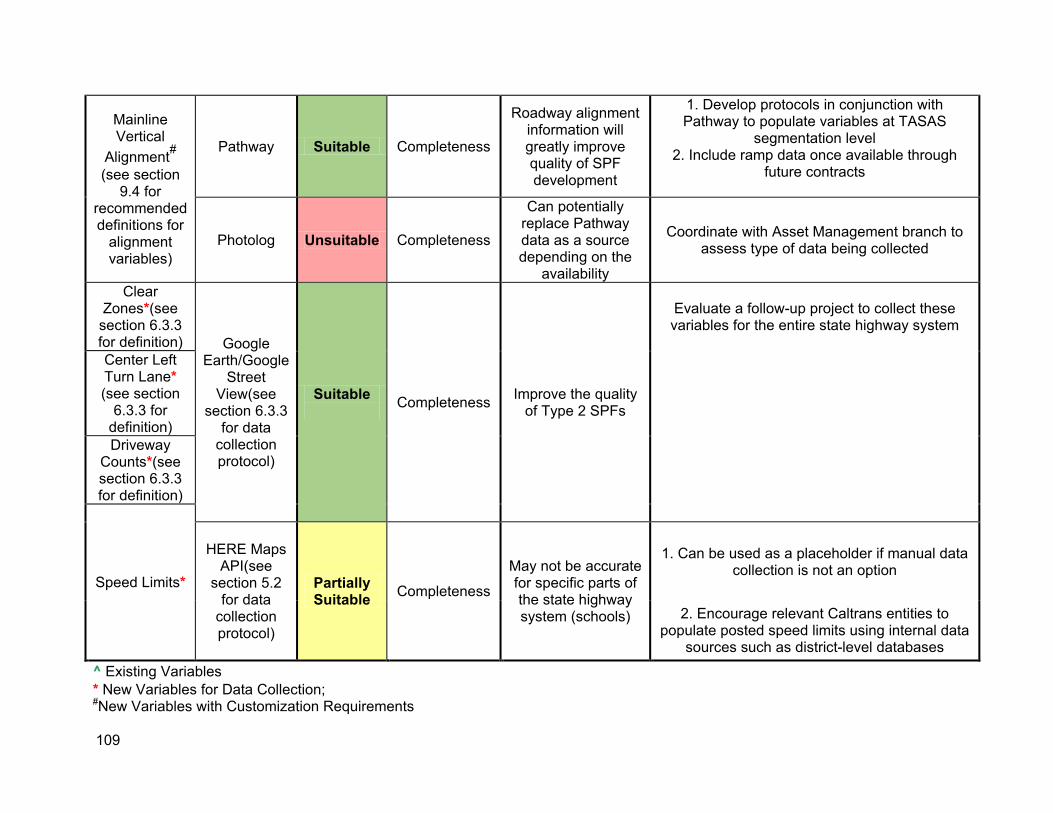
Mainline Vertical
Alignment#
(see section 9.4 for
recommended definitions for
alignment variables)
Pathway Suitable Completeness
Roadway alignment information will greatly improve quality of SPF development
1. Develop protocols in conjunction with Pathway to populate variables at TASAS
segmentation level 2. Include ramp data once available through
future contracts
Photolog Completeness
Can potentially replace Pathway data as a source depending on the
availability
Coordinate with Asset Management branch to assess type of data being collected Unsuitable
Clear Zones*(see
section 6.3.3 for definition) Google
Earth/Google Street
View(see section 6.3.3
for data collection protocol)
Completeness Improve the quality of Type 2 SPFs
Evaluate a follow-up project to collect these variables for the entire state highway system
Center Left Turn Lane* (see section
6.3.3 for definition)
Suitable
Driveway Counts*(see section 6.3.3 for definition)
Speed Limits*
HERE Maps API(see
section 5.2 for data
collection protocol)
PartiallySuitable Completeness
May not be accurate for specific parts of the state highway system (schools)
1. Can be used as a placeholder if manual data collection is not an option
2. Encourage relevant Caltrans entities to populate posted speed limits using internal data
sources such as district-level databases ^ Existing Variables * New Variables for Data Collection; #New Variables with Customization Requirements
109
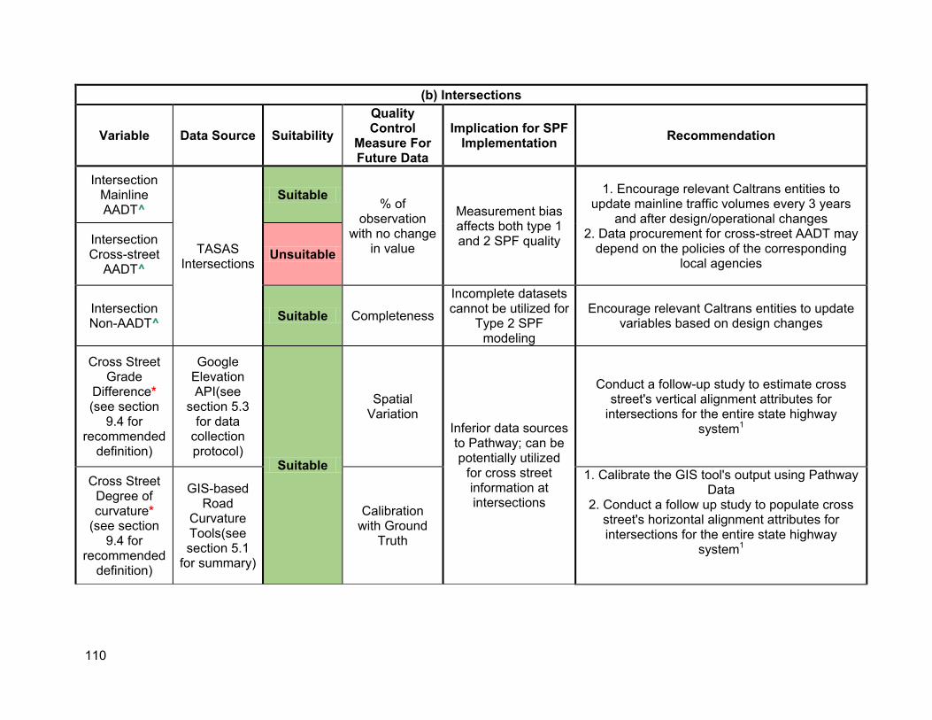
(b) Intersections
Variable Data Source Suitability QualityControl
Measure For Future Data
Implication for SPF Implementation Recommendation
Intersection Mainline AADT^
TASAS Intersections
Suitable % of
observation with no change
in value
Measurement bias affects both type 1 and 2 SPF quality
1. Encourage relevant Caltrans entities to update mainline traffic volumes every 3 years
and after design/operational changes 2. Data procurement for cross-street AADT may
depend on the policies of the corresponding local agencies
Intersection Cross-street
AADT^ Unsuitable
Intersection Non-AADT^ Suitable Completeness
Incomplete datasets cannot be utilized for
Type 2 SPF modeling
Encourage relevant Caltrans entities to update variables based on design changes
Cross Street Grade
Difference* (see section
9.4 for recommended
definition)
Google Elevation API(see
section 5.3 for data
collection protocol)
Suitable
Spatial Variation
Inferior data sources to Pathway; can be potentially utilized
for cross street information at intersections
Conduct a follow-up study to estimate cross street's vertical alignment attributes for
intersections for the entire state highway system1
Cross Street Degree of curvature*
(see section 9.4 for
recommended definition)
GIS-based Road
Curvature Tools(see section 5.1
for summary)
Calibration with Ground
Truth
1. Calibrate the GIS tool's output using Pathway Data
2. Conduct a follow up study to populate cross street's horizontal alignment attributes for intersections for the entire state highway
system1
110

Crosswalks*(s ee section 6.3.3 for
definition)
Google Earth/Google
Street View(see
section 6.3 for data
collection protocol)
Suitable Completeness Improves the quality of Type 2 SPFs
Evaluate a follow-up project to collect these variables for the entire state highway system
Speed Limits* HERE Maps
API PartiallySuitable Completeness
May not be accurate for specific parts of the state highway system (schools)
1. Can be used as a placeholder if manual data collection is not an option
2. Encourage relevant Caltrans entities to populate posted speed limits using internal data
sources such as district-level databases ^ Existing Variables * New Variables for Data Collection; #New Variables with Customization Requirements 1May need to include cross-street segments beyond 250 ft from centerline
(c) Ramps
Variable Data Source Suitability
Quality Control Measure For Future Data
Implication for SPF Implementation Recommendation
Ramp AADT^
TASAS Ramps Suitable
% of observation with no change in
value
Measurement bias affects both type 1 and 2 SPF
quality
Encourage relevant Caltrans entities to update traffic volumes every 3 years and after design/operational changes
Ramp Non-AADT^
TASAS Ramps Suitable Completeness
Incomplete datasets cannot be utilized for Type 2 SPF
modeling
Encourage relevant Caltrans entities to update variables based on design changes
^ Existing Variables
111

112
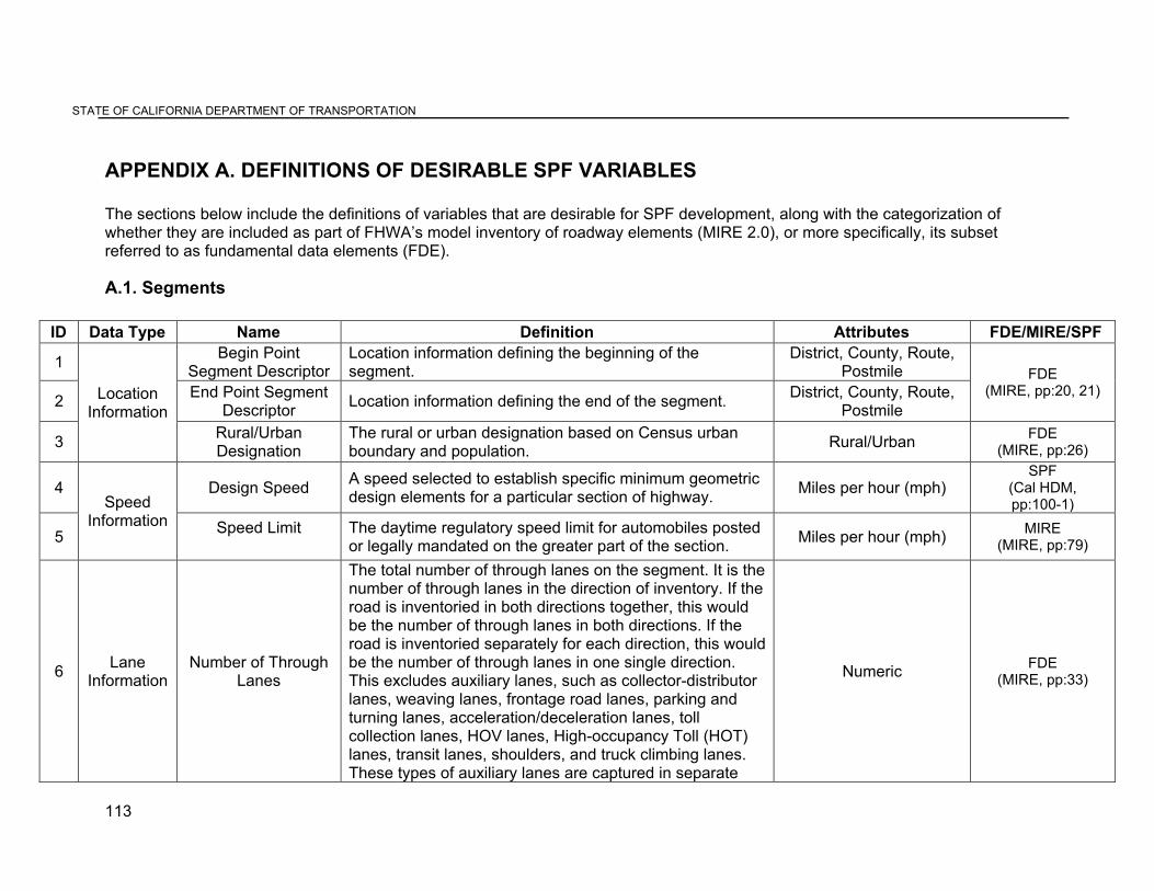
STATE OF CALIFORNIA DEPARTMENT OF TRANSPORTATION
APPENDIX A. DEFINITIONS OF DESIRABLE SPF VARIABLES
The sections below include the definitions of variables that are desirable for SPF development, along with the categorization of whether they are included as part of FHWA’s model inventory of roadway elements (MIRE 2.0), or more specifically, its subset referred to as fundamental data elements (FDE).
A.1. Segments
ID Data Type Name Definition Attributes FDE/MIRE/SPF
1 Begin Point Segment Descriptor
Location information defining the beginning of the segment.
District, County, Route, Postmile FDE
(MIRE, pp:20, 21) 2 Location
Information End Point Segment
Descriptor Location information defining the end of the segment. District, County, Route, Postmile
3 Rural/Urban Designation
The rural or urban designation based on Census urban boundary and population. Rural/Urban FDE
(MIRE, pp:26)
4 Speed
Design Speed A speed selected to establish specific minimum geometric design elements for a particular section of highway. Miles per hour (mph)
SPF (Cal HDM, pp:100-1)
5 Information Speed Limit The daytime regulatory speed limit for automobiles posted
or legally mandated on the greater part of the section. Miles per hour (mph) MIRE (MIRE, pp:79)
6 Lane Information
Number of Through Lanes
The total number of through lanes on the segment. It is the number of through lanes in the direction of inventory. If the road is inventoried in both directions together, this would be the number of through lanes in both directions. If the road is inventoried separately for each direction, this would be the number of through lanes in one single direction. This excludes auxiliary lanes, such as collector-distributor lanes, weaving lanes, frontage road lanes, parking and turning lanes, acceleration/deceleration lanes, toll collection lanes, HOV lanes, High-occupancy Toll (HOT) lanes, transit lanes, shoulders, and truck climbing lanes. These types of auxiliary lanes are captured in separate
Numeric FDE (MIRE, pp:33)
113
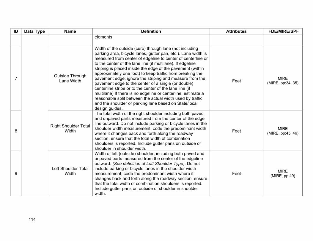
ID Data Type Name Definition Attributes FDE/MIRE/SPF elements.
7 Outside Through Lane Width
Width of the outside (curb) through lane (not including parking area, bicycle lanes, gutter pan, etc.). Lane width is measured from center of edgeline to center of centerline or to the center of the lane line (if multilane). If edgeline striping is placed inside the edge of the pavement (within approximately one foot) to keep traffic from breaking the pavement edge, ignore the striping and measure from the pavement edge to the center of a single (or double) centerline stripe or to the center of the lane line (if multilane) If there is no edgeline or centerline, estimate a reasonable split between the actual width used by traffic and the shoulder or parking lane based on State/local design guides.
Feet MIRE (MIRE, pp:34, 35)
8 Right Shoulder Total
Width
The total width of the right shoulder including both paved and unpaved parts measured from the center of the edge line outward. Do not include parking or bicycle lanes in the shoulder width measurement; code the predominant width where it changes back and forth along the roadway section; ensure that the total width of combination shoulders is reported. Include gutter pans on outside of shoulder in shoulder width.
Feet MIRE (MIRE, pp:45, 46)
9 Left Shoulder Total
Width
Width of left (outside) shoulder, including both paved and unpaved parts measured from the center of the edgeline outward. (See definition of Left Shoulder Type). Do not include parking or bicycle lanes in the shoulder width measurement; code the predominant width where it changes back and forth along the roadway section; ensure that the total width of combination shoulders is reported. Include gutter pans on outside of shoulder in shoulder width.
Feet MIRE (MIRE, pp:49)
114
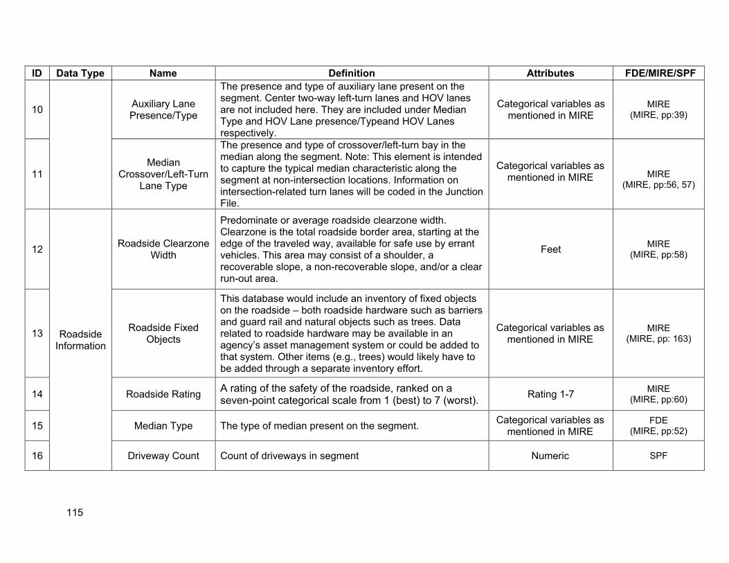
ID Data Type Name Definition Attributes FDE/MIRE/SPF
10 Auxiliary Lane Presence/Type
The presence and type of auxiliary lane present on the segment. Center two-way left-turn lanes and HOV lanes are not included here. They are included under Median Type and HOV Lane presence/Typeand HOV Lanes respectively.
Categorical variables as mentioned in MIRE
MIRE (MIRE, pp:39)
11 Median
Crossover/Left-Turn Lane Type
The presence and type of crossover/left-turn bay in the median along the segment. Note: This element is intended to capture the typical median characteristic along the segment at non-intersection locations. Information on intersection-related turn lanes will be coded in the Junction File.
Categorical variables as mentioned in MIRE MIRE
(MIRE, pp:56, 57)
12
Roadside Information
Roadside Clearzone Width
Predominate or average roadside clearzone width. Clearzone is the total roadside border area, starting at the edge of the traveled way, available for safe use by errant vehicles. This area may consist of a shoulder, a recoverable slope, a non-recoverable slope, and/or a clear run-out area.
Feet MIRE (MIRE, pp:58)
13 Roadside Fixed Objects
This database would include an inventory of fixed objects on the roadside – both roadside hardware such as barriers and guard rail and natural objects such as trees. Data related to roadside hardware may be available in an agency’s asset management system or could be added to that system. Other items (e.g., trees) would likely have to be added through a separate inventory effort.
Categorical variables as mentioned in MIRE
MIRE (MIRE, pp: 163)
14 Roadside Rating A rating of the safety of the roadside, ranked on a seven-point categorical scale from 1 (best) to 7 (worst). Rating 1-7 MIRE
(MIRE, pp:60)
15 Median Type The type of median present on the segment. Categorical variables as mentioned in MIRE
FDE (MIRE, pp:52)
16 Driveway Count Count of driveways in segment Numeric SPF
115
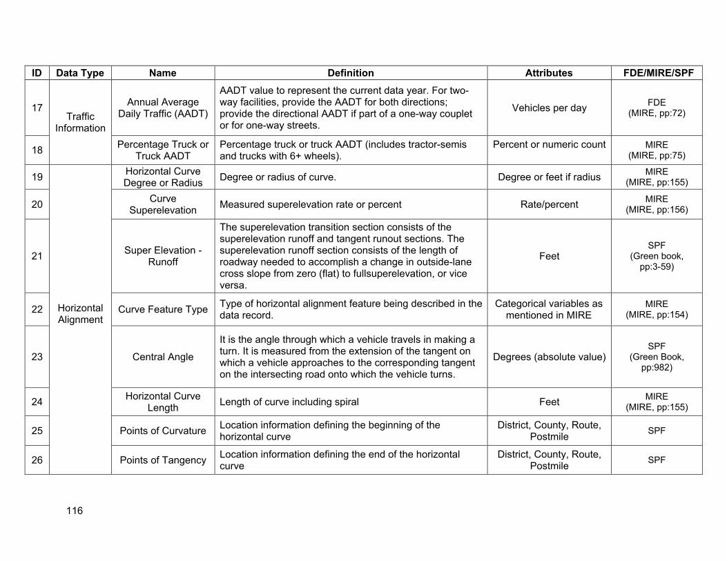
ID Data Type Name Definition Attributes FDE/MIRE/SPF
17 Traffic
Information
Annual Average Daily Traffic (AADT)
AADT value to represent the current data year. For two-way facilities, provide the AADT for both directions; provide the directional AADT if part of a one-way couplet or for one-way streets.
Vehicles per day FDE (MIRE, pp:72)
18 Percentage Truck or Truck AADT
Percentage truck or truck AADT (includes tractor-semis and trucks with 6+ wheels).
Percent or numeric count MIRE (MIRE, pp:75)
19
Horizontal Alignment
Horizontal Curve Degree or Radius Degree or radius of curve. Degree or feet if radius MIRE
(MIRE, pp:155)
20 Curve Superelevation Measured superelevation rate or percent Rate/percent MIRE
(MIRE, pp:156)
21 Super Elevation -Runoff
The superelevation transition section consists of the superelevation runoff and tangent runout sections. The superelevation runoff section consists of the length of roadway needed to accomplish a change in outside-lane cross slope from zero (flat) to fullsuperelevation, or vice versa.
Feet SPF
(Green book, pp:3-59)
22 Curve Feature Type Type of horizontal alignment feature being described in the data record.
Categorical variables as mentioned in MIRE
MIRE (MIRE, pp:154)
23 Central Angle
It is the angle through which a vehicle travels in making a turn. It is measured from the extension of the tangent on which a vehicle approaches to the corresponding tangent on the intersecting road onto which the vehicle turns.
Degrees (absolute value) SPF
(Green Book, pp:982)
24 Horizontal Curve Length Length of curve including spiral Feet MIRE
(MIRE, pp:155)
25 Points of Curvature Location information defining the beginning of the horizontal curve
District, County, Route, Postmile SPF
26 Points of Tangency Location information defining the end of the horizontal curve
District, County, Route, Postmile SPF
116
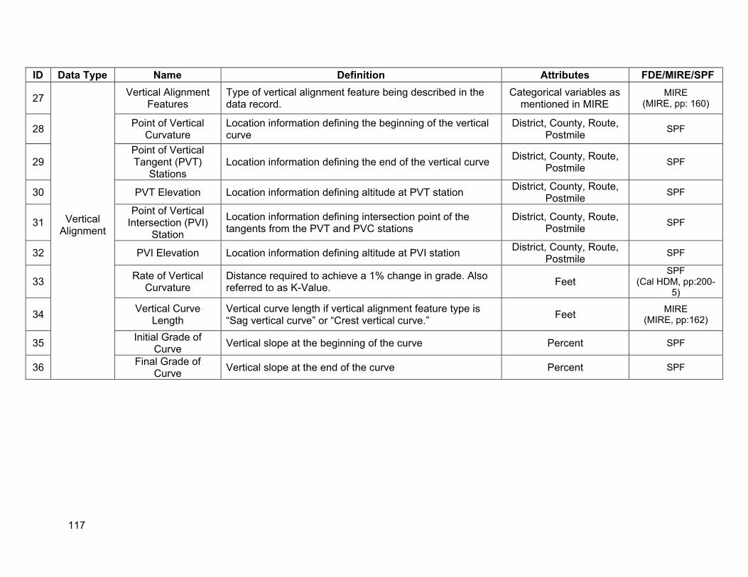
27
28
29
30
31
32
33
34
35
36
ID Data Type Name Definition Attributes FDE/MIRE/SPF
Vertical Alignment
Vertical Alignment Features
Type of vertical alignment feature being described in the data record.
Categorical variables as mentioned in MIRE
MIRE (MIRE, pp: 160)
Point of Vertical Curvature
Location information defining the beginning of the vertical curve
District, County, Route, Postmile SPF
Point of Vertical Tangent (PVT)
Stations Location information defining the end of the vertical curve District, County, Route,
Postmile SPF
PVT Elevation Location information defining altitude at PVT station District, County, Route, Postmile SPF
Point of Vertical Intersection (PVI)
Station
Location information defining intersection point of the tangents from the PVT and PVC stations
District, County, Route, Postmile SPF
PVI Elevation Location information defining altitude at PVI station District, County, Route, Postmile SPF
Rate of Vertical Curvature
Distance required to achieve a 1% change in grade. Also referred to as K-Value. Feet
SPF (Cal HDM, pp:200-
5)
Vertical Curve Length
Vertical curve length if vertical alignment feature type is “Sag vertical curve” or “Crest vertical curve.” Feet MIRE
(MIRE, pp:162)
Initial Grade of Curve Vertical slope at the beginning of the curve Percent SPF
Final Grade of Curve Vertical slope at the end of the curve Percent SPF
117
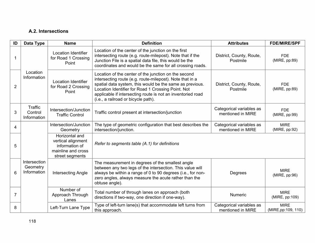
A.2. Intersections
ID Data Type Name Definition Attributes FDE/MIRE/SPF
1
Location Information
Location Identifier for Road 1 Crossing
Point
Location of the center of the junction on the first intersecting route (e.g. route-milepost). Note that if the Junction File is a spatial data file, this would be the coordinates and would be the same for all crossing roads.
District, County, Route, Postmile
FDE (MIRE, pp:89)
2 Location Identifier
for Road 2 Crossing Point
Location of the center of the junction on the second intersecting route (e.g. route-milepost). Note that in a spatial data system, this would be the same as previous. Location Identifier for Road 1 Crossing Point. Not applicable if intersecting route is not an inventoried road (i.e., a railroad or bicycle path).
District, County, Route, Postmile
FDE (MIRE, pp:89)
3 Traffic Control
Information
Intersection/Junction Traffic Control Traffic control present at intersection/junction
Categorical variables as mentioned in MIRE
FDE (MIRE, pp:99)
4
Intersection Geometry
Information
Intersection/Junction Geometry
The type of geometric configuration that best describes the intersection/junction.
Categorical variables as mentioned in MIRE
MIRE (MIRE, pp:92)
5
Horizontal and vertical alignment
information of mainline and cross
street segments
Refer to segments table (A.1) for definitions
6 Intersecting Angle
The measurement in degrees of the smallest angle between any two legs of the intersection. This value will always be within a range of 0 to 90 degrees (i.e., for non-zero angles, always measure the acute rather than the obtuse angle).
Degrees MIRE (MIRE, pp:96)
7 Number of
Approach Through Lanes
Total number of through lanes on approach (both directions if two-way, one direction if one-way). Numeric MIRE
(MIRE, pp:109)
8 Left-Turn Lane Type Type of left-turn lane(s) that accommodate left turns from this approach.
Categorical variables as mentioned in MIRE
MIRE (MIRE,pp:109, 110)
118
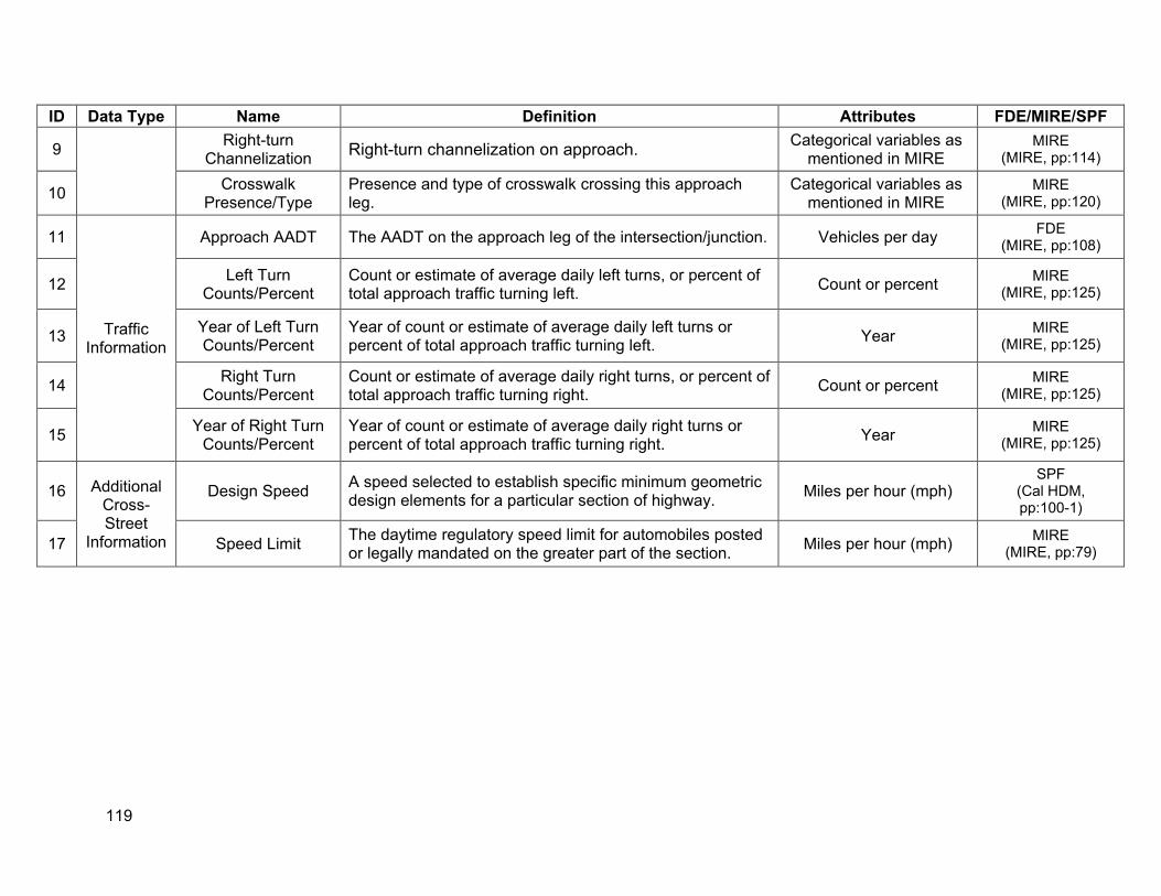
9
10
11
12
13
14
15
16
17
ID Data Type Name Definition Attributes FDE/MIRE/SPF Right-turn
Channelization Right-turn channelization on approach. Categorical variables as mentioned in MIRE
MIRE (MIRE, pp:114)
Crosswalk Presence/Type
Presence and type of crosswalk crossing this approach leg.
Categorical variables as mentioned in MIRE
MIRE (MIRE, pp:120)
Traffic Information
Approach AADT The AADT on the approach leg of the intersection/junction. Vehicles per day FDE (MIRE, pp:108)
Left Turn Counts/Percent
Count or estimate of average daily left turns, or percent of total approach traffic turning left. Count or percent MIRE
(MIRE, pp:125)
Year of Left Turn Counts/Percent
Year of count or estimate of average daily left turns or percent of total approach traffic turning left. Year MIRE
(MIRE, pp:125)
Right Turn Counts/Percent
Count or estimate of average daily right turns, or percent of total approach traffic turning right. Count or percent MIRE
(MIRE, pp:125)
Year of Right Turn Counts/Percent
Year of count or estimate of average daily right turns or percent of total approach traffic turning right. Year MIRE
(MIRE, pp:125)
Additional Cross-Street
Information
Design Speed A speed selected to establish specific minimum geometric design elements for a particular section of highway. Miles per hour (mph)
SPF (Cal HDM, pp:100-1)
Speed Limit The daytime regulatory speed limit for automobiles posted or legally mandated on the greater part of the section. Miles per hour (mph) MIRE
(MIRE, pp:79)
119
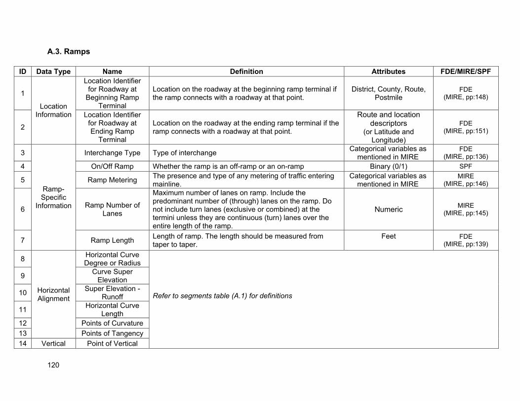
A.3. Ramps
ID Data Type Name Definition Attributes FDE/MIRE/SPF
1
Location Information
Location Identifier for Roadway at
Beginning Ramp Terminal
Location on the roadway at the beginning ramp terminal if the ramp connects with a roadway at that point.
District, County, Route, Postmile
FDE (MIRE, pp:148)
2
Location Identifier for Roadway at Ending Ramp
Terminal
Location on the roadway at the ending ramp terminal if the ramp connects with a roadway at that point.
Route and location descriptors
(or Latitude and Longitude)
FDE (MIRE, pp:151)
3
Ramp-Specific
Information
Interchange Type Type of interchange Categorical variables as mentioned in MIRE
FDE (MIRE, pp:136)
4 On/Off Ramp Whether the ramp is an off-ramp or an on-ramp Binary (0/1) SPF
5 Ramp Metering The presence and type of any metering of traffic entering mainline.
Categorical variables as mentioned in MIRE
MIRE (MIRE, pp:146)
6 Ramp Number of Lanes
Maximum number of lanes on ramp. Include the predominant number of (through) lanes on the ramp. Do not include turn lanes (exclusive or combined) at the termini unless they are continuous (turn) lanes over the entire length of the ramp.
Numeric MIRE (MIRE, pp:145)
7 Ramp Length Length of ramp. The length should be measured from taper to taper.
Feet FDE (MIRE, pp:139)
8
Horizontal Alignment
Horizontal Curve Degree or Radius
Refer to segments table (A.1) for definitions
9 Curve Super Elevation
10 Super Elevation -Runoff
11 Horizontal Curve Length
12 Points of Curvature 13 Points of Tangency 14 Vertical Point of Vertical
120
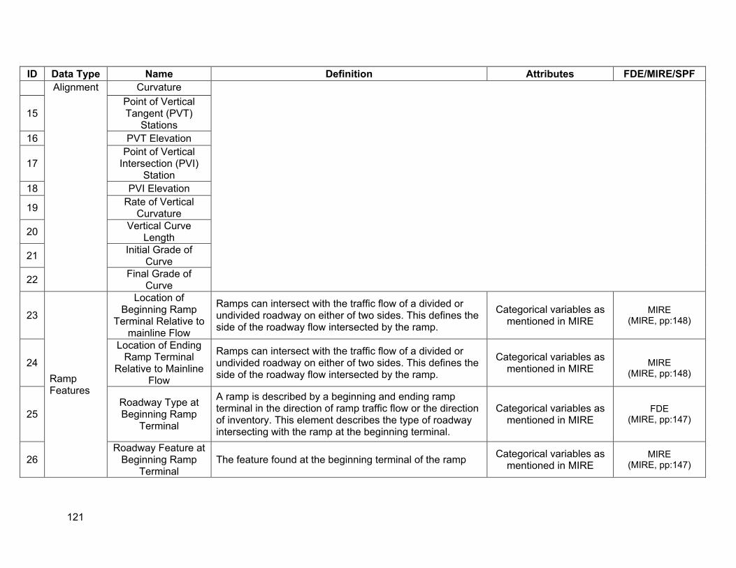
ID Data Type Name Definition Attributes FDE/MIRE/SPF Alignment Curvature
15 Point of Vertical Tangent (PVT)
Stations 16 PVT Elevation
17 Point of Vertical
Intersection (PVI) Station
18 PVI Elevation
19 Rate of Vertical Curvature
20 Vertical Curve Length
21 Initial Grade of Curve
22 Final Grade of Curve
23
Ramp Features
Location of Beginning Ramp
Terminal Relative to mainline Flow
Ramps can intersect with the traffic flow of a divided or undivided roadway on either of two sides. This defines the side of the roadway flow intersected by the ramp.
Categorical variables as mentioned in MIRE
MIRE (MIRE, pp:148)
24
Location of Ending Ramp Terminal
Relative to Mainline Flow
Ramps can intersect with the traffic flow of a divided or undivided roadway on either of two sides. This defines the side of the roadway flow intersected by the ramp.
Categorical variables as mentioned in MIRE MIRE
(MIRE, pp:148)
25 Roadway Type at Beginning Ramp
Terminal
A ramp is described by a beginning and ending ramp terminal in the direction of ramp traffic flow or the direction of inventory. This element describes the type of roadway intersecting with the ramp at the beginning terminal.
Categorical variables as mentioned in MIRE
FDE (MIRE, pp:147)
26 Roadway Feature at
Beginning Ramp Terminal
The feature found at the beginning terminal of the ramp Categorical variables as mentioned in MIRE
MIRE (MIRE, pp:147)
121
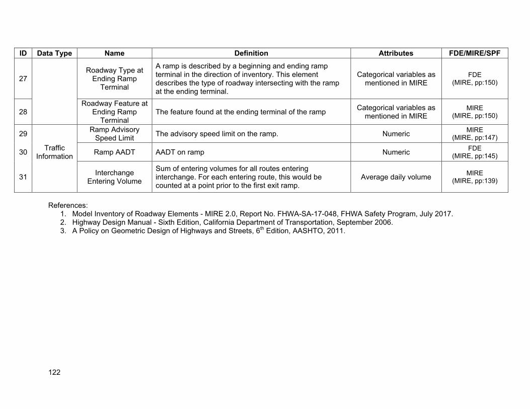
ID Data Type Name Definition Attributes FDE/MIRE/SPF
27 Roadway Type at
Ending Ramp Terminal
A ramp is described by a beginning and ending ramp terminal in the direction of inventory. This element describes the type of roadway intersecting with the ramp at the ending terminal.
Categorical variables as mentioned in MIRE
FDE (MIRE, pp:150)
28 Roadway Feature at
Ending Ramp Terminal
The feature found at the ending terminal of the ramp Categorical variables as mentioned in MIRE
MIRE (MIRE, pp:150)
29 Ramp Advisory Speed Limit The advisory speed limit on the ramp. Numeric MIRE
(MIRE, pp:147)
30 Traffic Information Ramp AADT AADT on ramp Numeric FDE
(MIRE, pp:145)
31 Interchange Entering Volume
Sum of entering volumes for all routes entering interchange. For each entering route, this would be counted at a point prior to the first exit ramp.
Average daily volume MIRE (MIRE, pp:139)
References: 1. Model Inventory of Roadway Elements - MIRE 2.0, Report No. FHWA-SA-17-048, FHWA Safety Program, July 2017. 2. Highway Design Manual - Sixth Edition, California Department of Transportation, September 2006. 3. A Policy on Geometric Design of Highways and Streets, 6th Edition, AASHTO, 2011.
122
Related Documents