Taylor Introms10 Ppt 16

16-1Copyright © 2010 Pearson Education, Inc. Publishing as Prentice Hall

Inventory Management

Chapter 16

16-2

Elements of Inventory Management Inventory Control Systems Economic Order Quantity Models The Basic EOQ Model The EOQ Model with Non-Instantaneous Receipt The EOQ Model with Shortages EOQ Analysis with QM for Windows EOQ Analysis with Excel and Excel QM Quantity Discounts Reorder Point Determining Safety Stocks Using Service Levels Order Quantity for a Periodic Inventory System

Chapter Topics

Copyright © 2010 Pearson Education, Inc. Publishing as Prentice Hall

16-3

Inventory is a stock of items kept on hand used to meet customer demand..

A level of inventory is maintained that will meet anticipated demand.

If demand not known with certainty, safety (buffer) stocks are kept on hand.

Additional stocks are sometimes built up to meet seasonal or cyclical demand.

Large amounts of inventory sometimes purchased to take advantage of discounts.

Elements of Inventory ManagementRole of Inventory (1 of 2)


16-4

In-process inventories maintained to provide independence between operations.

Raw materials inventory kept to avoid delays in case of supplier problems.

Stock of finished parts kept to meet customer demand in event of work stoppage.

In general inventory serves to decouple consecutive steps.

Elements of Inventory ManagementRole of Inventory (2 of 2)


16-5

Inventory exists to meet the demand of customers. Customers can be external (purchasers of

products) or internal (workers using material). Management needs an accurate forecast of

demand. Items that are used internally to produce a final

product are referred to as dependent demand items.

Items that are final products demanded by an external customer are independent demand items.

Elements of Inventory Management Demand


16-6

Carrying costs - Costs of holding items in storage. Vary with level of inventory and sometimes with

length of time held. Include facility operating costs, record keeping,

interest, etc. Assigned on a per unit basis per time period, or

as percentage of average inventory value (usually estimated as 10% to 40%).

Elements of Inventory ManagementInventory Costs (1 of 3)


16-7

Ordering costs - costs of replenishing stock of inventory. Expressed as dollar amount per order,

independent of order size. Vary with the number of orders made. Include purchase orders, shipping, handling,

inspection, etc.



16-8

Shortage (stockout ) costs - Associated with insufficient inventory. Result in permanent loss of sales and profits for

items not on hand. Sometimes penalties involved; if customer is

internal, work delays could result.



16-9

An inventory control system controls the level of inventory by determining how much (replenishment level) and when to order.

Two basic types of systems -continuous (fixed-order quantity) and periodic (fixed-time). In a continuous system, an order is placed for

the same constant amount when inventory decreases to a specified level.

In a periodic system, an order is placed for a variable amount after a specified period of time.

Inventory Control Systems


16-10

A continual record of inventory level is maintained. Whenever inventory decreases to a predetermined

level, the reorder point, an order is placed for a fixed amount to replenish the stock.

The fixed amount is termed the economic order quantity, whose magnitude is set at a level that minimizes the total inventory carrying, ordering, and shortage costs.

Because of continual monitoring, management is always aware of status of inventory level and critical parts, but system is relatively expensive to maintain.

Inventory Control SystemsContinuous Inventory Systems


16-11

Inventory on hand is counted at specific time intervals and an order placed that brings inventory up to a specified level.

Inventory not monitored between counts and system is therefore less costly to track and keep account of.

Results in less direct control by management and thus generally higher levels of inventory to guard against stockouts.

System requires a new order quantity each time an order is placed.

Used in smaller retail stores, drugstores, grocery stores and offices.

Inventory Control SystemsPeriodic Inventory Systems


16-12

Economic order quantity, or economic lot size, is the quantity ordered when inventory decreases to the reorder point.

Amount is determined using the economic order quantity (EOQ) model.

Purpose of the EOQ model is to determine the optimal order size that will minimize total inventory costs.

Three model versions to be discussed:

1. Basic EOQ model

2. EOQ model without instantaneous receipt

3. EOQ model with shortages

Economic Order Quantity Models


16-13

A formula for determining the optimal order size that minimizes the sum of carrying costs and ordering costs.

Simplifying assumptions and restrictions:

Demand is known with certainty and is relatively constant over time.

No shortages are allowed.

Lead time for the receipt of orders is constant.

The order quantity is received all at once and instantaneously.

Economic Order Quantity ModelsBasic EOQ Model (1 of 2)


16-14

Figure 16.1 The Inventory Order Cycle

Economic Order Quantity ModelsBasic EOQ Model (2 of 2)


16-15

Carrying cost usually expressed on a per unit basis of time, traditionally one year.

Annual carrying cost equals carrying cost per unit per year times average inventory level:

Carrying cost per unit per year = Cc

Average inventory = Q/2

Annual carrying cost = CcQ/2.

Basic EOQ ModelCarrying Cost (1 of 2)


16-16

Figure 16.4 Average Inventory

Basic EOQ ModelCarrying Cost (2 of 2)


16-17

Total annual ordering cost equals cost per order (Co) times number of orders per year.

Number of orders per year, with known and constant demand, D, is D/Q, where Q is the order size:

Annual ordering cost = CoD/Q

Only variable is Q, Co and D are constant parameters.

Relative magnitude of the ordering cost is dependent on order size.

Basic EOQ ModelOrdering Cost


16-18

2QcCQ

DoCTC

Total annual inventory cost is sum of ordering and carrying cost:

Basic EOQ ModelTotal Inventory Cost (1 of 2)


16-19

Figure 16.5 The EOQ Cost Model

Basic EOQ ModelTotal Inventory Cost (2 of 2)


16-20

EOQ occurs where total cost curve is at minimum value and carrying cost equals ordering cost:

The EOQ model is robust because Q is a square root and errors in the estimation of D, Cc and Co are dampened.

min 2

2

QC D optoTC CcQopt

C DoQopt Cc

Basic EOQ ModelEOQ and Minimum Total Cost


16-21

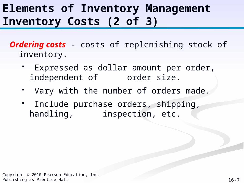
Model parameters:

C $0.75, C $150, D 10,000ydc o

Optimal order size:

2 2(150)(10,000) 2,000 yd(0.75)

C DoQopt Cc

I-75 Carpet Discount Store, Super Shag carpet sales.

Given following data, determine number of orders to be made annually and time between orders given store is open every day except Sunday, Thanksgiving Day, and Christmas Day.

Basic EOQ ModelExample (1 of 2)


16-22

Total annual inventory cost:

(2,000)10,000(150) (0.75) $1,500min 2 2,000 2

Number of orders per year:

10,000 52,000

311 days 311Order cycle time 62.2 store days5/

QoptDTC C Co cQopt

DQopt

D Qopt

Basic EOQ ModelExample (2 of 2)


16-23

Model parameters:

C $0.0625 per yd per monthcC $150 per orderoD 833.3 yd per month

Optimal order size:

2 2(150)(833.3) 2,000 yd(0.0625)

C DoQopt Cc

For any time period unit of analysis, EOQ is the same.

Shag Carpet example on monthly basis:

Basic EOQ ModelEOQ Analysis Over Time (1 of 2)


16-24

Total monthly inventory cost:

min 2

(833.3) (2,000)(150) (0.0625)2,000 2

$125 per month

Total annual inventory cost ($125)(12) $1,500

QoptDTC C Co cQopt

Basic EOQ ModelEOQ Analysis Over Time (2 of 2)


16-25

In the non-instantaneous receipt model the assumption that orders are received all at once is relaxed. (Also known as gradual usage or production lot size model.)

The order quantity is received gradually over time and inventory is drawn on at the same time it is being replenished.

EOQ ModelNon-Instantaneous Receipt Description (1 of 2)


16-26

Figure 16.6 The EOQ Model with Non-Instantaneous Order Receipt

EOQ ModelNon-Instantaneous Receipt Description (2 of 2)


16-27

p daily rate at which the order is received over timed daily rate at which inventory is demanded

Maximum inventory level 1

Average inventory level 12

Total carrying cost

dQ p

Q dp

12

Total annual inventory cost 12

Q dC pc

QD dC C po cQ

Non-Instantaneous Receipt ModelModel Formulation (1 of 2)


16-28

1 at lowest point of total cost curve2

2Optimal order size:

(1 / )

Q d DC Cpc oQ

C DoQopt C d pc

Non-Instantaneous Receipt ModelModel Formulation (2 of 2)


16-29

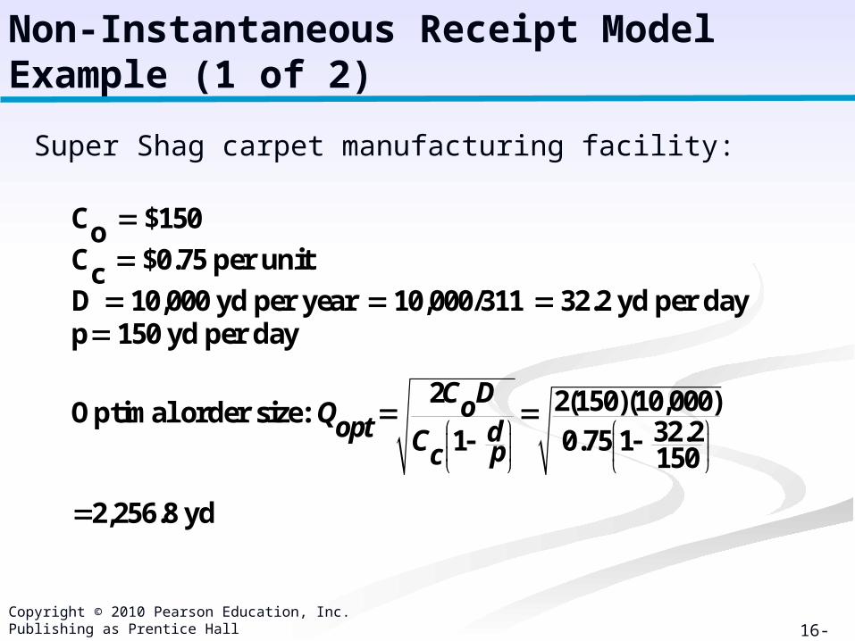
C $150oC $0.75 per unitcD 10,000 yd per year 10,000/311 32.2 yd per dayp 150 yd per day

2 2(150)(10,000)Optimal order size: 32.21 0.75 1150

2,256.8 yd

C DoQopt dC pc

Non-Instantaneous Receipt ModelExample (1 of 2)

Super Shag carpet manufacturing facility:


16-30

Total minimum annual inventory cost 12

(10,000) (2,256.8) 32.2(150) (.075) 1 $1,329(2,256.8) 2 150

2,256.8Production run length 15.05 days150

Number of orders per year (prod

QD dC C po cQ

Qp

uction runs)

10,000 4.43 runs2,256.8

32.2Maximum inventory level 1 2,256.8 1 1,772 yd150

DQ

dQ p

Non-Instantaneous Receipt ModelExample (2 of 2)


16-31

EOQ Model with ShortagesDescription (1 of 2)

In the EOQ model with shortages, the assumption that shortages cannot exist is relaxed.

Assumed that unmet demand can be backordered with all demand eventually satisfied.


16-32

Figure 16.7 The EOQ Model with Shortages

EOQ Model with ShortagesDescription (2 of 2)


16-33

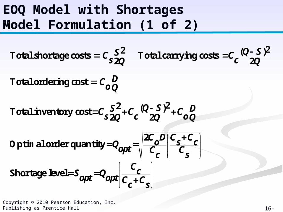
22 ( )Total shortage costs Total carrying costs 2 2

Total ordering cost

22 ( )Total inventory cost2 2

2Optimal order quantity

Shortage lev

Q SSC Cs cQ Q

DCoQ

Q SS DC C Cs c oQ Q Q

C D C Co s cQopt C Cc s

elCcS Qopt opt C Cc s

EOQ Model with ShortagesModel Formulation (1 of 2)


16-34

Figure 16.8 Cost Model with Shortages



16-35

C $150oC $0.75 per ydcC $2 per ydsD 10,000 yd

Optimal order quantity:

2 2(150)(10,000) 2 0.75 2,345.2 yd0.75 2

C D C Co s cQopt C Cc s


I-75 Carpet Discount Store allows shortages; shortage cost Cs, is $2/yard per year.


16-36

Shortage level:

0.752,345.2 639.6 yd2 0.75

Total inventory cost:

22 ( )2 2

2 2(2)(639.6) (0.75)(1,705.6) (150)(10,000)2(2,345.2) 2(2,345.2) 2,345.2

$17

CcS Qopt opt C Cc s

Q SS DTC C C Cs c oQ Q Q

4.44 465.16 639.60 $1,279.20



16-37

10,000Number of orders 4.26 orders per year2,345.2

Maximum inventory level 2,345.2 639.6 1,705.6 yd

days per year 311Time between orders t 73.0 daysnumber of orders 4.26

Time during which

DQ

Q S

inventory is on hand

2,345.2-639.6 t 0.171 or 53.2 days1 10,000

Time during which there is a shortage

639.6 t 0.064 year or 19.9 daysD2 10,000

Q SD

S



16-38


Exhibit 16.1

EOQ Analysis with QM for Windows

16-39

Exhibit 16.2

EOQ Analysis with Excel and Excel QM (1 of 2)


16-40

Exhibit 16.3

EOQ Analysis with Excel and Excel QM (2 of 2)


16-41

Price discounts are often offered if a predetermined number of units is ordered or when ordering materials in high volume.

Basic EOQ model used with purchase price added:

where: P = per unit price of the item D = annual demand

Quantity discounts are evaluated under two different scenarios:

With constant carrying costs

With carrying costs as a percentage of purchase price

2QDTC C C PDo cQ

Quantity Discounts


16-42

Quantity Discounts with Constant Carrying Costs Analysis Approach

Optimal order size is the same regardless of the discount price.

The total cost with the optimal order size must be compared with any lower total cost with a discount price to determine which is the lesser.


16-43

University bookstore: For following discount schedule offered by Comptek, should bookstore buy at the discount terms or order the basic EOQ order size?

Determine optimal order size and total cost:

Quantity Price 1- 49 50 – 89 90 +

$1,400 1,100 900

Quantity Discounts with Constant Carrying CostsExample (1 of 2)

C $2,500 C $190 per unit D 200o c

2C D 2(2,500)(200)oQ 72.5opt C 190c


16-44

Compute total cost at eligible discount price ($1,100):

Compare with total cost of with order size of 90 and price of $900:

Because $194,105 < $233,784, maximum discount price should be taken and 90 units ordered.

min 2

(2,500)(200) (72.5) (190) (1,100)(200) $233,784(72.5) 2

QC D optoTC C PDcQopt

2(2,500)(200) (190)(90) (900)(200) $194,105

(90) 2

C D QoTC C PDcQ

Quantity Discounts with Constant Carrying CostsExample (2 of 2)


16-45

University Bookstore example, but a different optimal order size for each price discount.

Optimal order size and total cost determined using basic EOQ model with no quantity discount.

This cost then compared with various discount quantity order sizes to determine minimum cost order.

This must be compared with EOQ-determined order size for specific discount price.

Data:

Co = $2,500 D = 200 computers per year

Quantity Discounts with Carrying CostsPercentage of Price Example (1 of 3)


16-46

Compute optimum order size for purchase price without discount and Cc = $210:

Compute new order size:

Quantity Price Carrying Cost

0 - 49 $1,400 1,400(.15) = $210

50 - 89 1,100 1,100(.15) = 165

90 + 900 900(.15) = 135


2 2(2,500)(200) 69210

C DoQopt Cc

2(2,500)(200) 77.8165

Qopt


16-47

Compute minimum total cost:

Compare with cost, discount price of $900, order quantity of 90:

Optimal order size computed as follows:

Since this order size is less than 90 units , it is not feasible, thus optimal order size is 90 units.

(2,500)(200) (77.8)165 (1,100)(200)2 77.8 2

$232,845

C D QoTC C PDcQ

(2,500)(200) (135)(90) (900)(200) $191,63090 2

TC

2(2,500)(200) 86.1135

Qopt



16-48

Exhibit 16.4

Quantity Discount ModelSolution with QM for Windows


16-49

Quantity Discount ModelSolution with QM for Windows

Exhibit 16.5Copyright © 2010 Pearson Education, Inc. Publishing as Prentice Hall

16-50

The reorder point is the inventory level at which a new order is placed.

Order must be made while there is enough stock in place to cover demand during lead time.

Formulation:

R = dL

where d = demand rate per time period

L = lead time

For Carpet Discount store problem:

R = dL = (10,000/311)(10) = 321.54

Reorder Point (1 of 4)


16-51

Figure 16.9 Reorder Point and Lead Time



16-52

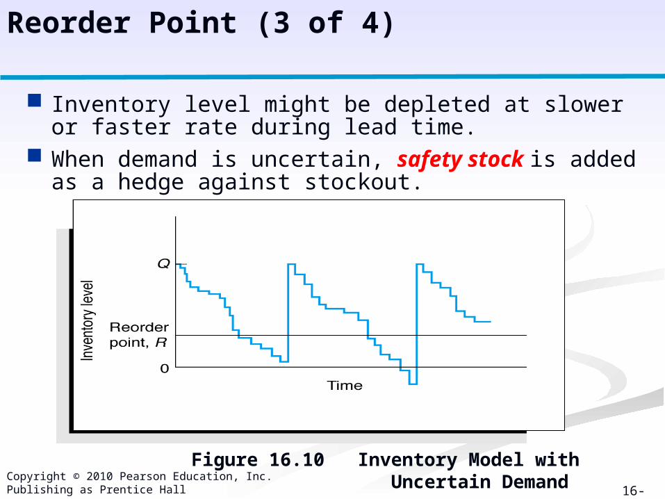
Figure 16.10 Inventory Model with Uncertain Demand


Inventory level might be depleted at slower or faster rate during lead time.

When demand is uncertain, safety stock is added as a hedge against stockout.


16-53

Figure 16.11 Inventory model with safety stock



16-54

Determining Safety Stocks Using Service Levels

Service level is probability that amount of inventory on hand is sufficient to meet demand during lead time (probability stockout will not occur).

The higher the probability inventory will be on hand, the more likely customer demand will be met.

Service level of 90% means there is a .90 probability that demand will be met during lead time and .10 probability of a stockout.


16-55

where:

reorder point

average daily demand

lead time

the standard deviation of daily demand

number of standard deviations corresponding to service level probability

sa

R dL Z Ld

R

d

L

d

Z

Z Ld

fety stock

Reorder Point with Variable Demand (1 of 2)


16-56

Figure 16.12 Reorder Point for a Service Level

Reorder Point with Variable Demand (2 of 2)


16-57

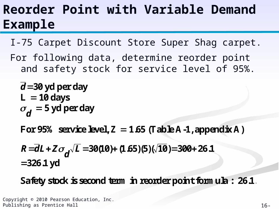
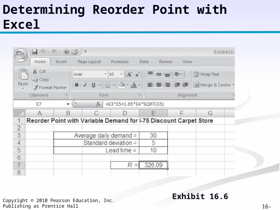
30 yd per dayL 10 days

5 yd per day

For 95% service level, Z 1.65 (Table A-1, appendix A)

30(10) (1.65)(5)( 10) 300 26.1

326.1 yd

Safety stock is second term in reorder point formula :

d

d

R dL Z Ld

26.1.

I-75 Carpet Discount Store Super Shag carpet.

For following data, determine reorder point and safety stock for service level of 95%.

Reorder Point with Variable Demand Example


16-58

Exhibit 16.6

Determining Reorder Point with Excel


16-59

where:

constant daily demand average lead time standard deviation of lead time

standard deviation of demand during lead time

safety stock

R dL ZdL

dL

LdL

ZdL

Reorder Point with Variable Lead Time

For constant demand and variable lead time:


16-60

30 yd per day

10 days

3 days

1.65 for a 95% service level

(30)(10) (1.65)(30)(3)300 148.5448.5 yd

d

L

L

Z

R dL ZdL

Reorder Point with Variable Lead Time Example

Carpet Discount Store:


16-61

22 2( ) ( )

where: average daily demand average lead time

2 2 2( ) ( ) standard deviation

of demand during lead time

2Z ( ) ( )

R dL Z L dLd

dL

L dLd

LLd

2 2

safety stockd

When both demand and lead time are variable:

Reorder PointVariable Demand and Lead Time


16-62

30 yd per day 5 yd per day

10 days3 days

1.65 for 95% service level

22 2( ) ( )

(30)(10) (1.65) (5)(5)(10) (3)(3)(30)(30) 300 150.8 450.8 yds

d

dL

LZ

R dL Z L dLd

Carpet Discount Store:

Reorder PointVariable Demand and Lead Time Example


16-63

Order Quantity for a Periodic Inventory System

A periodic, or fixed-time period inventory system is one in which time between orders is constant and the order size varies.

Vendors make periodic visits, and stock of inventory is counted.

An order is placed, if necessary, to bring inventory level back up to some desired level.

Inventory not monitored between visits.

At times, inventory can be exhausted prior to the visit, resulting in a stockout.

Larger safety stocks are generally required for the periodic inventory system.


16-64

For normally distributed variable daily demand:

( )

where:

average demand rate the fixed time between orders

lead time standard deviation of demand

safety stock

inventory in stock

Q d t L Z t L Ib d b

dtbL

dZ t Ld b

I

Order Quantity for Variable Demand


16-65

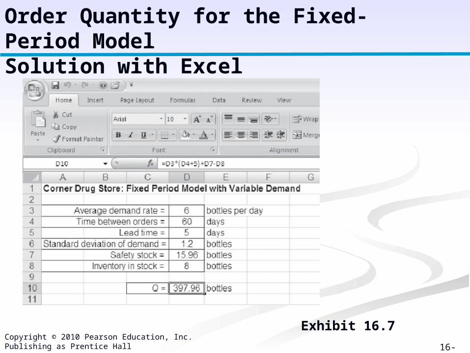
6 bottles per day 1.2 bottles

60 days

5 days 8 bottles 1.65 for 95% service level

( )

(6)(60 5) (1.65)(1.2) 60 5 8 398 bottles

d

dtbLIZ

Q d t L Z t L Ib d b

Corner Drug Store with periodic inventory system.

Order size to maintain 95% service level:

Order Quantity for Variable Demand Example


16-66

Exhibit 16.7

Order Quantity for the Fixed-Period ModelSolution with Excel


16-67

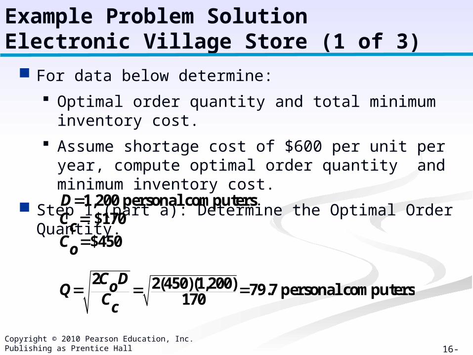
For data below determine:

Optimal order quantity and total minimum inventory cost.

Assume shortage cost of $600 per unit per year, compute optimal order quantity and minimum inventory cost.

Step 1 (part a): Determine the Optimal Order Quantity.

Example Problem SolutionElectronic Village Store (1 of 3)

1,200 personal computers $170

$450

2 2(450)(1,200) 79.7 personal computers170

DCcCo

C DoQCc


16-68

Step 2 (part b): Compute the EOQ with Shortages.

1,20079.7Total cost 170 4502 2 79.7

$13,549.91

Q DC Cc oQ


$600

2 2(450)(1200) 600 170170 600

90.3 personal computers

Cs

C D C Co s cQC Cc s


16-69


17090.3 19.9 personal computers170 600

2 2( )Total cost 2 2

2 2(600)(19.9) (90.3 19.9) 1,200170 4502(90.3) 2(90.3) 90.3

$11,960.98

CcS QC Cc s

C S C DQ Ss oCcQ Q Q


16-70

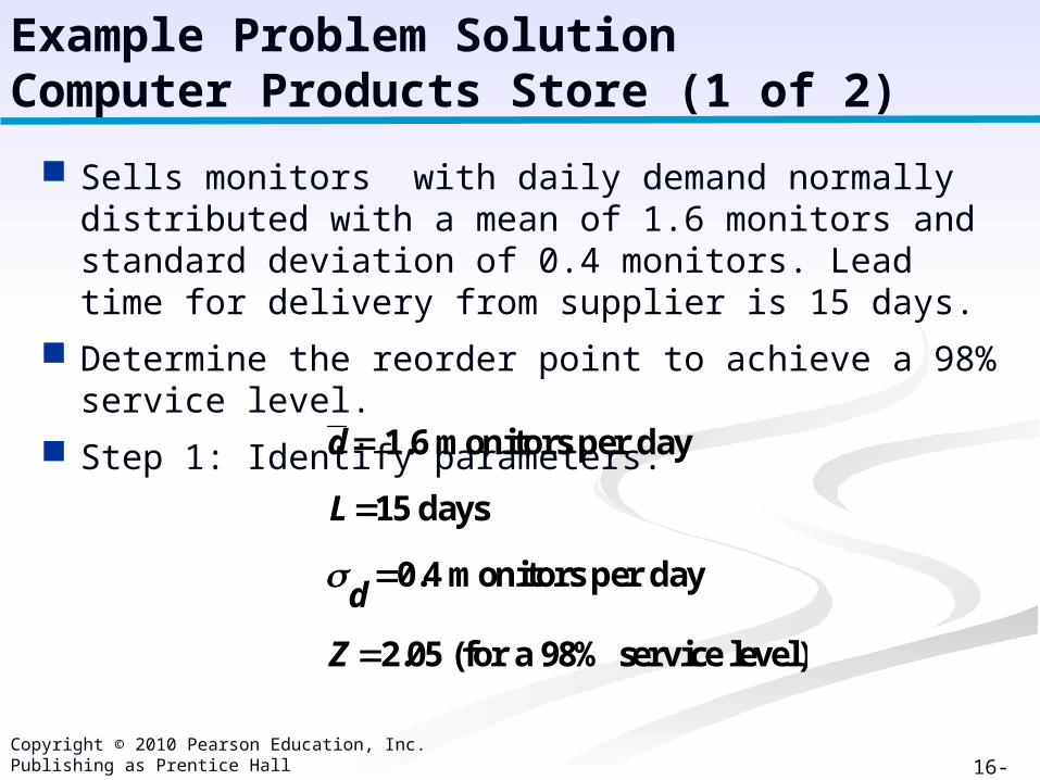
1.6 monitors per day

15 days

0.4 monitors per day

2.05 (for a 98% service level)

d

L

d

Z

Example Problem SolutionComputer Products Store (1 of 2)

Sells monitors with daily demand normally distributed with a mean of 1.6 monitors and standard deviation of 0.4 monitors. Lead time for delivery from supplier is 15 days.

Determine the reorder point to achieve a 98% service level.

Step 1: Identify parameters.


16-71

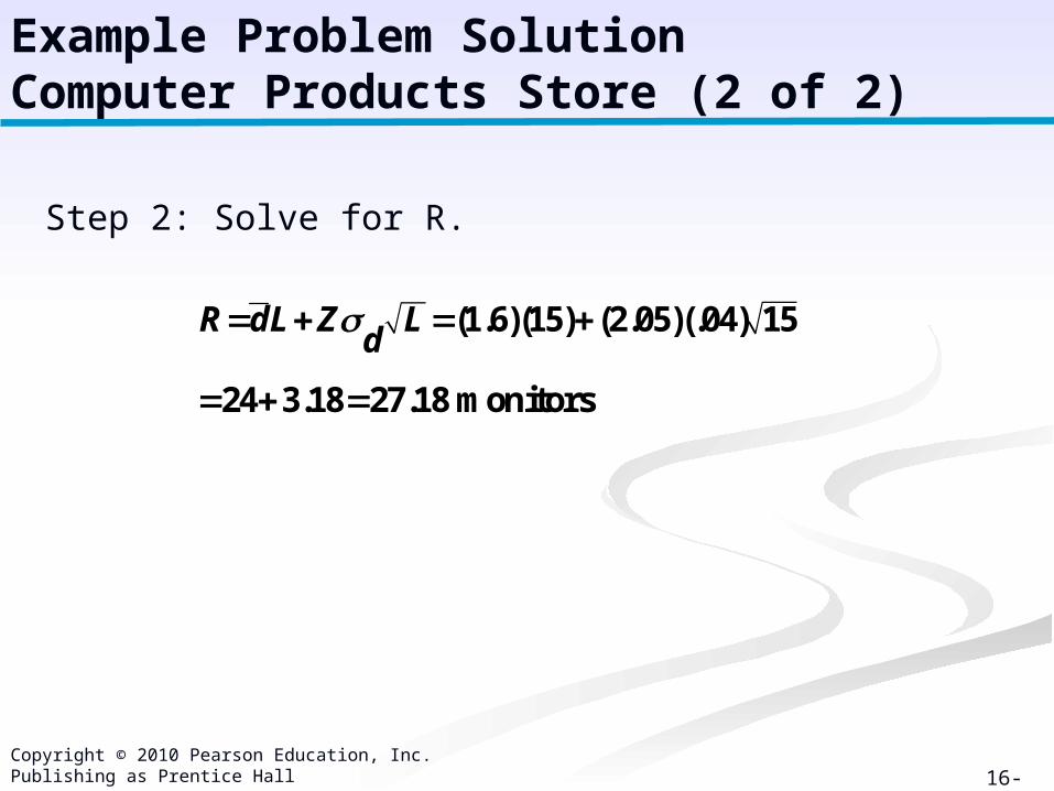
Example Problem SolutionComputer Products Store (2 of 2)

Step 2: Solve for R.

(1.6)(15) (2.05)(.04) 15

24 3.18 27.18 monitors

R dL Z Ld


16-72


Taylor Introms10 Ppt 16

Documents

instantaneous

optimal order

instantaneous

basic eoq

economic order

shortages

inventory

carrying costs