Taxonomic Classification of Bacterial 16S rRNA Genes Using ...

Taxonomic Classification of Bacterial 16S rRNA GenesUsing Short Sequencing Reads: Evaluation of EffectiveStudy DesignsOrna Mizrahi-Man, Emily R. Davenport, Yoav Gilad*

Department of Human Genetics, University of Chicago, Chicago, Illinois, United States of America

Abstract

Massively parallel high throughput sequencing technologies allow us to interrogate the microbial composition of biologicalsamples at unprecedented resolution. The typical approach is to perform high-throughout sequencing of 16S rRNA genes,which are then taxonomically classified based on similarity to known sequences in existing databases. Current technologiescause a predicament though, because although they enable deep coverage of samples, they are limited in the length ofsequence they can produce. As a result, high-throughout studies of microbial communities often do not sequence theentire 16S rRNA gene. The challenge is to obtain reliable representation of bacterial communities through taxonomicclassification of short 16S rRNA gene sequences. In this study we explored properties of different study designs anddeveloped specific recommendations for effective use of short-read sequencing technologies for the purpose ofinterrogating bacterial communities, with a focus on classification using naıve Bayesian classifiers. To assess precision andcoverage of each design, we used a collection of ,8,500 manually curated 16S rRNA gene sequences from cultured bacteriaand a set of over one million bacterial 16S rRNA gene sequences retrieved from environmental samples, respectively. Wealso tested different configurations of taxonomic classification approaches using short read sequencing data, and providerecommendations for optimal choice of the relevant parameters. We conclude that with a judicious selection of thesequenced region and the corresponding choice of a suitable training set for taxonomic classification, it is possible toexplore bacterial communities at great depth using current technologies, with only a minimal loss of taxonomic resolution.

Citation: Mizrahi-Man O, Davenport ER, Gilad Y (2013) Taxonomic Classification of Bacterial 16S rRNA Genes Using Short Sequencing Reads: Evaluation ofEffective Study Designs. PLoS ONE 8(1): e53608. doi:10.1371/journal.pone.0053608

Editor: Bryan A White, University of Illinois, United States of America

Received August 14, 2012; Accepted December 3, 2012; Published January 7, 2013

Copyright: � 2013 Mizrahi-Man et al. This is an open-access article distributed under the terms of the Creative Commons Attribution License, which permitsunrestricted use, distribution, and reproduction in any medium, provided the original author and source are credited.

Funding: This work was supported by NIH grant HL092206 to YG, and by a pilot and feasibility DDRC grant (Digestive Diseases Research Core Center) to YG,funded by P30DK42086. The funders had no role in study design, data collection and analysis, decision to publish, or preparation of the manuscript.

Competing Interests: The authors have declared that no competing interests exist.

* E-mail: [email protected]

Introduction

Originally proposed by Woese and Fox, the classification of

ribosomal RNA genes has been the gold standard for molecular

taxonomic research for decades [1,2]. The 16S small ribosomal

subunit gene (16S rRNA), in particular, has been widely used to

study and characterize bacterial community compositions in a

variety of ecological niches including host associated communities,

such as the endogenous human microbiome [3–5], and host-free

communities, such as soil and ocean environments [6,7]. Several

aspects of the 16S rRNA gene make it optimal as a marker for

these types of studies. First, it is ubiquitous among prokaryotic life.

Second, its size and high degree of functional conservation result

in clock-like mutation rates throughout prokaryotic evolution [8].

Third, and most importantly, the 16S rRNA gene includes both

conserved regions, which can be used for designing amplification

primers across taxa, as well as nine hypervariable regions (V1-V9),

which can be effectively used to distinguish between taxa [9].

Early bacterial community studies typically sequenced the entire

16S rRNA gene, but their ability to sample the full array of

bacterial diversity was limited by depth of sequencing. With the

advent of massively parallel sequencing technologies, which

generally yield short reads, focus has shifted from sequencing the

full 16S rRNA gene to sequencing shorter sub-regions of the gene

at great depth [10–12]. Of the second-generation sequencing

platforms, large-scale pyrosequencing (454) was the preferred

choice initially, as it provides somewhat longer reads (up to

500 bp) compared to other platforms. However, recently, other

platforms (such as the Illumina MiSEQ and HiSEQ) have become

much more attractive for microbiome studies due to increase in

sequencing read length (to ,100 bp at the moment and up to

,250 bp next year) combined with a much higher and cheaper

output [10,13–15]. Though the microbiome field is experiencing a

shift in the choice of sequencing technology there has not been a

systematic evaluation of the properties of alternative study designs

that utilize these technologies.

Several studies have examined different aspects of short read

study designs for 16S classification by analyzing the effects of

variation in read length, region choice, and sampling depth [16–

23]. However, results from these studies are often conflicting

[16,18–23] and a standard design for bacterial community studies

has not yet emerged (e.g., different studies sequence different 16S

rRNA gene regions). In addition, the rapid pace at which

sequencing technologies are evolving requires frequent evaluation

and modifications of the optimal study designs. A common

framework that would facilitate the evaluation, comparison, and

PLOS ONE | www.plosone.org 1 January 2013 | Volume 8 | Issue 1 | e53608

optimal parameterization of different experimental designs in

terms of precision and coverage is not yet available.

There are three properties of bacterial community studies using

short sequencing read technologies that principally determine the

extent to which the study is effective. First, the specific sequencing

strategy (e.g., read length, single or paired end); second, the choice

of 16S rRNA gene regions to be sequenced; third, the choice of

taxonomic classifier. Most studies of bacterial communities to date

used 454 sequencing (relatively long reads, which can include

more than one 16S rRNA gene hypervariable region, but

relatively low depth). However, recently several studies have used

deep, short-read, single-end Illumina sequencing, with few studies

using paired-end sequencing but analyzing the data without taking

into account the paired-end structure of the reads [10,13,14,24–

29]. With the rise in the use of Illumina short-read sequencing for

bacterial community studies, it is important to now rigorously

examine these three properties mentioned above in a systematic

and comprehensive way to develop sequencing strategies appro-

priate for this platform.

The first property, sequencing strategy, has not been fully

examined in the literature. Although several studies of 16S rRNA

gene sequencing study design looked at various read lengths

[11,19,21], many of these read lengths were chosen based on the

capacities of 454 technology, and are not ideal for short, Illumina

length reads. In addition, few studies have taken into account the

ability for Illumina reads to be paired-end [11,21,29]. In a recent

study, Werner et al [29] examined the merits of paired-end

sequencing as compared to single-end sequencing, but rather than

classifying their reads to a known taxonomy, the authors clustered

their data into operational taxonomic units (OTUs) and calculated

diversity indices, as well as built a phylogenetic tree from these

OTUs. Finally, the limitations of insert size have not been

considered in various studies. For example, Soergel, et al. [21]

recently examined combinations of primers spanning the full

region of the 16S rRNA gene, without taking into account that

some of these products after amplification would be longer than

the generally accepted 400–600 bp insert size recommendations

for Illumina sequences.

Several bioinformatics studies have examined the second

property, namely the choice of 16S rRNA gene region [11,18–

21,23]. Most extensive among these was the recent study by

Soergel et al [21], which examined thousands of primer and read

length combinations, but unfortunately focused only on queries

that had a close counterpart (at least 97% identity) in the reference

database. As a result, there is no way of knowing how the

experimental designs examined would perform on novel species,

which are common in environmental surveys. This and other

studies have come to differing conclusions on the most effective

hypervariable region to target, with recommendations including

one or more of the V2, V3, V4, V6 or V3/V4 regions. These

differences in results are possibly due to many factors including

specific primers examined, the environmental source of the reads,

and classification method and parameters chosen during analysis.

This lack of consensus is apparent in recent literature, with most

current studies focusing on either hypervariable region V3, V4 or

V6 [10,28,30–33], with no convergence on a single hypervariable

region being chosen.

With regards to the third property, the choice of classifier, there

are three varieties of algorithms to choose from. One category of

tools, classifies 16S rRNA gene fragments based on sequence

alignment based similarity. Notable in this category is the GAST

[18] program, which was specifically designed with short gene

fragments in mind. A second category of tools, including for

example pplacer [34], attempts to find the correct location of the

gene fragment within a phylogenetic tree of the reference

sequences. The third category of tools uses word composition to

assign taxonomy to a read. Algorithms in this category include

nearest-neighbor searches as in SimRank [35] and SeqMatch [23]

and naıve Bayesian classifiers, such as the ribosomal database

project (RDP) classifier [23] and Mothur’s classify.seq function

[36]. Liu et al [19] performed a comprehensive comparison

among methods from all three of these categories (but did not

include GAST [18] or pplacer [34], which had not published yet

at the time) and recommended the RDP classifier [23] and

SimRank [35] for the accuracy and stability of their results, with

RDP classifier being the most efficient of the methods examined in

terms of run time. Despite not being designed for short sequences,

for a number of primers these classifiers showed excellent recovery

and coverage even for 100 nt sequences [19]. Indeed, naıve

Bayesian classifiers have been a popular choice for the analysis of

high throughput sequencing reads (for example, [31,37–39]). We

therefore decided to focus on naıve Bayesian classifiers for our

analyses.

As mentioned above, available naıve Bayesian classifiers were

originally developed to classify full-length 16S rRNA gene

sequences and have not yet been thoroughly evaluated and

optimized for use with short sequencing reads. In particular, the

default use of the RDP classifier utilizes a training set of full 16S

rRNA gene sequences, which might be suboptimal for the purpose

of classifying short reads. Indeed, it has been suggested that

trimming the selected training set down from the full-length 16S

rRNA gene to the size of the sequenced region improves the

performance of the classifier [40].

There is also the issue of determining confidence score cutoffs

for classification. Rather than reporting the probability that a

prediction is correct, all current implementations of naıve Bayesian

classifiers provide a confidence score for each level of the

classification, with the intuitive interpretation of low scores being

that a given sequence could belong to one of several taxa with

almost equal probability. These confidence scores, however,

cannot be directly translated to probabilities of error. The original

recommendation of the RDP classifier developers, which is widely

used in the literature, was to use a confidence score threshold of 80

regardless of the taxonomic level that is being classified, and this is

the default threshold for this classifier [23]. Claesson et al. [16]

compared the performance of this default threshold with a

threshold of 50% in the classification of subsequences from three

hypervariable regions, using a sample of near full-length sequences

from the human gut. Subsequently the RDP developers adopted

Claesson et al.’s [16] recommendation to use a threshold of 50 for

the classification of 16S rRNA gene fragments of length 50–

250 nt, regardless of the 16S rRNA gene region that is being

sequenced (or the taxonomic rank) (http://rdp.cme.msu.edu/

classifier/class_help.jsp#conf). Most studies published to date that

used a naıve Bayesian classifier for taxonomic classification utilized

50% or 80% as a confidence threshold. Ultimately, we wish to

understand confidence score thresholds in terms of estimates of

false negative and positive rates, or false discovery rates.

Confidence thresholds should be chosen that balance precision

and coverage.

In this study, we synthesize ideas and analyses that cover the

range of all three principle properties that determine effectiveness

in study design, incorporating these various parameters into a

unified, comprehensive study aimed at determining the most

effective 16S rRNA gene based assays for short-read second

generation sequencers. We present a bioinformatic analysis, using

a naıve Bayesian classifier, of various study designs for short read

bacterial community experiments, exploring different sequencing

Evaluation of Effective Microbiome Study Designs


strategies, 16S rRNA gene regions, and training sets, and

examining the relationship between confidence scores, false

discovery rates, and overall coverage. We offer recommendations

for an effective bacterial community study design given the

capabilities of current technologies, as well as propose a framework

that allows one to optimize the parameters of the study design

when new technologies emerge.

Results and Discussion

A Framework for the Comparison of ClassificationPerformance

Our goal was to compare the performance of bacterial

community study designs using different regions of the 16S rRNA

gene to classify sequences into known bacterial taxa. Previous

studies evaluating alternative experimental designs did so using

one [11,18,19] or very few parameter settings [16,21]. Optimal

classification performance balances precision and coverage.

Therefore, to obtain a complete view when comparing the

effectiveness of different experimental designs we wished to

evaluate their performance while varying the classifier parameters.

To this end we devised a framework in which classification

performance was evaluated for both precision and coverage. In the

current study we used this framework to evaluate the classification

by the naıve Bayesian classifier of sequencing configurations

typical of the current capabilities of the Illumina platform.

However, the same evaluation framework can be generalized

and applied to any classifier and experimental configuration.

The first consideration in the framework we propose is a

stringent method to evaluate the precision of the classifier being

tested. A typical approach is the leave-one-out cross-validation

method, which requires just one set of sequences. In each iteration

all sequences but one are used for training, and the sequence left

out is being classified [19,23]. However, the training set is a

parameter of the classifier, for which one may wish to evaluate

several options. For a fair comparison in our study, we need to

settle on one ‘‘test set’’ with known taxonomy that can be used

across all tests. We selected the ,8,500 bacterial sequences and

their corresponding taxonomic annotation from ‘‘The All-Species

Living Tree’’ project (LTP; [41,42]) as a test set, considering each

time only the subsequences relevant for the experimental design in

question. Then, to evaluate precision we used a leave-k-out

approach, whereby, in each iteration, we removed from the

training set all sequences of the species to be classified (see

Methods for more details). This is a rather conservative approach,

as previous studies excluded from training only the particular

tested sequence [19,23]). In addition, We also included all

sequences in the evaluation, regardless of their distance from the

closest match in the training database (instead of following the

common approach of retaining only sequences with at least 97%

identity with the closest match [21]). In turn, to evaluate and

compare coverage across the different training sets, we used a set

of more than a million environmental (uncultured) bacterial

sequences (available through the RDP database [43,44]), focusing

on the subsequences relevant to the experimental design (see

Methods for more details).

The second major aspect of our framework was to assess the

precision of the classifier in terms of false prediction rates of

classification of our sequences. The naıve Bayesian classifier

accompanies each prediction with a bootstrap confidence value.

However, the same bootstrap value obtained by the naıve

Bayesian classifier may result in different precision and coverage

for different taxonomic ranks, as well as for different regions

[16,19]. Thus, to obtain a complete view of the relationship

between precision and coverage we explored in this study the full

range of bootstrap confidence values. In the analyses that follow,

the distribution of confidence values obtained in the leave-k-out

tests was skewed towards high confidence values (Figure S1),

probably because most test sequences are associated with densely

sampled regions of bacterial phylogeny. In order to draw

conclusions that would be applicable to any set of sequences,

irrespective of the distribution of confidence values, we used a pre-

defined set of precision values and determined conservative

thresholds that would ensure these precisions at a minimum (see

Methods). We then used these thresholds to compute coverage in

environmental sequences.

Diverse Training Sets Afford Better PerformanceThe basis for taxonomic classification of unknown 16S rRNA

gene sequences is a training set of sequences with known

taxonomy. We tested out several different training sets in order

to select the set with best performance for short reads. We

reasoned that the optimal training set would be current and

accurate in terms of underlying taxonomy, as well as diverse,

containing sequences representing all bacteria cultured to date.

We compared the performance of the RDP training set v. 6 (‘RDP

TS6’), which is the built-in training set for RDP classifier [23] and

thus the most commonly used training set when classifying 16S

Table 1. Training sets used for the naıve Bayesian classification of bacterial 16S rRNA gene sequences.

Abbreviation Description Sequence Databasea Underlying Taxonomy

RDP TS6 RDP classifier training set v.6 (default forv. 2.3 of the RDP classifier)

8,127 bacterial and 295 archaealsequences

Based on ‘‘The Taxonomic Outline ofBacteria and Archaea’’ (TOBA) 7.7 [52]

LTP Bacterial subset of ‘‘The Living TreeProject’’ v. 106

8,494 bacterial sequences ‘‘List of Prokaryotic names with Standingin Nomenclature (LPSN; http://www.bacterio.cict.fr/)

unfiltered RDP All bacterial isolates in RDP database 31,334 non-redundant bacterialsequencesb

Based on ‘‘The Taxonomic Outline ofBacteria and Archaea’’ (TOBA) 7.7 [52]

filtered NCBI All bacterial isolates in RDP database,filtered for annotation quality

21,240 non-redundant bacterialsequencesb

NCBI taxonomy [48]

aExcept for the ‘RDP TS6’ training set, which always trains on the full sequence, numbers are only for the testing of 100 nt single-reads from the V4 region. For the threeother training sets, which train only on the region to be classified, the number of sequences reflects both the number of sequences covering this region (all threetraining sets) and its degree of redundancy (‘unfiltered RDP’ and ‘filtered NCBI’).bThe numbers are for the ‘original non-redundant training set’ (see Methods section ‘Leave k out classification testing’); numbers for each leave-k-out iteration may varyslightly.doi:10.1371/journal.pone.0053608.t001



rRNA genes using a naıve Bayesian classifier, to that of three

alternative sets (Table 1). ‘RDP TS6’ is comprised of ,8,500

mostly bacterial, type strain sequences, and therefore includes only

a fraction of the diversity currently available in 16S rRNA gene

databases. The bacterial portion of the taxonomic hierarchy

underlying this training set was last updated in 2008 [44].

The first alternative, the living tree project (LTP) training set,

was comprised of the ,8,500 bacterial sequences used as a test set

for precision, and emphasized both quality and currency, with

diversity comparable to that of the ‘RDP TS6’. Second, the

‘unfiltered RDP’ training set was comprised of all bacterial isolate

sequences available in the RDP database [43,44]. This training set

thus had the same taxonomic hierarchy as the ‘RDP TS6’ and is

highly diverse. Third, the ‘filtered NCBI’ training set was

comprised of the same sequences as the ‘unfiltered RDP’ training

set, but was filtered for quality and currency of annotation (see

Methods) and used the NCBI taxonomic annotation. This set is

potentially the most current and accurate of all three, yet only

slightly less diverse than the ‘unfiltered RDP’ training set. Finally,

in contrast to ‘RDP TS6’, which is comprised of full-length

sequences, all three alternative training sets were comprised of

only short, partial 16S rRNA gene sequences (in our case, the

sequences corresponding to the region to be classified).

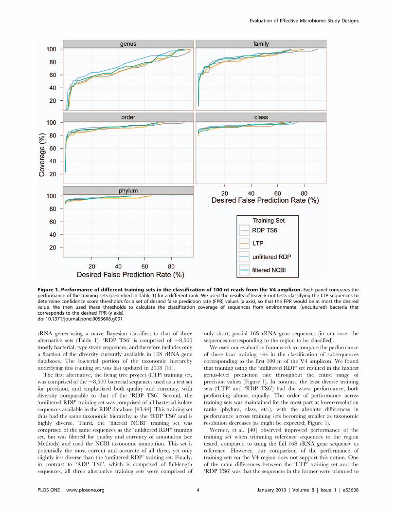
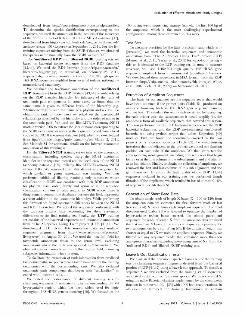
We used our evaluation framework to compare the performance

of these four training sets in the classification of subsequences

corresponding to the first 100 nt of the V4 amplicon. We found

that training using the ‘unfiltered RDP’ set resulted in the highest

genus-level prediction rate throughout the entire range of

precision values (Figure 1). In contrast, the least diverse training

sets (‘LTP’ and ‘RDP TS6’) had the worst performance, both

performing almost equally. The order of performance across

training sets was maintained for the most part at lower-resolution

ranks (phylum, class, etc.), with the absolute differences in

performance across training sets becoming smaller as taxonomic

resolution decreases (as might be expected; Figure 1).

Werner, et al. [40] observed improved performance of the

training set when trimming reference sequences to the region

tested, compared to using the full 16S rRNA gene sequence as

reference. However, our comparison of the performance of

training sets on the V4 region does not support this notion. One

of the main differences between the ‘LTP’ training set and the

‘RDP TS6’ was that the sequences in the former were trimmed to

Figure 1. Performance of different training sets in the classification of 100 nt reads from the V4 amplicon. Each panel compares theperformance of the training sets (described in Table 1) for a different rank. We used the results of leave-k-out tests classifying the LTP sequences todetermine confidence score thresholds for a set of desired false prediction rate (FPR) values (x axis), so that the FPR would be at most the desiredvalue. We then used these thresholds to calculate the classification coverage of sequences from environmental (uncultured) bacteria thatcorresponds to the desired FPR (y axis).doi:10.1371/journal.pone.0053608.g001



the region to be classified, whereas the latter contained full-length

sequences. Nevertheless, these two training sets displayed similar

performance. As an additional assessment of the effect of trimming

of training set sequences, we compared the performance of

training sets composed of sequences trimmed to the exact region

used for classification (i.e. the region that would be sequenced) or

to the complete amplicon (,250 nt; see Methods). The two

trimming regimes yielded practically identical results (Figures S2,

S3 and S4). This observation indicates that, at least for the

particular region we examined (V4), the composition of relatively

short sequence stretches in the vicinity of the region used for

classification is not a confounding factor. Because we had only

compared trimming regimes in one region and in other regions

using the full sequence or complete amplicon might still contribute

noise, in downstream analyses we chose to trim the training

sequences down to the region used for classification.

To further examine the performance of these four training sets

and confirm our choice we sequenced, using Illumina technology,

102 bp single-end reads of the V4 region from two human fecal

samples. We classified the reads using each of the four training

sets, setting for each training set and rank a confidence threshold

that would ensure at most 5% false predictions (Table 2; see

Methods). While coverage differed significantly between the two

samples, the ‘unfiltered RDP’ obtained the highest or second-

highest coverage for all ranks but class (nine and three cases,

respectively). Differences in performance among the training sets

were quite dramatic at the higher-resolution ranks, especially at

the genus level where training sets differed in performance by as

much as 26% in the classification of sample B reads.

Thus, in line with the results of Werner, et al. [40], we found

that the defining feature of a good training set is its diversity. Even

a current, quality-filtered and relatively diverse training set

(‘filtered NCBI’) performed poorly compared with the most

diverse training set, which is less current and unfiltered for quality

(‘unfiltered RDP’). Similarly, the ‘LTP’ training set and the ‘RDP

TS6’, which contained similar numbers of sequences, performed

equivalently, despite the fact that the taxonomy of the former is

more current. This is perhaps because the sequence data available

for novel taxa are too sparse. As more near-full-length sequences

accumulate for the novel taxa it may become important to use a

current taxonomy.

Given these observations, for subsequent exploration of different

parameters of bacterial community study designs, we used the

‘unfiltered RDP’ training set, restricting the training in each case

to the short 16S rRNA gene region that would be sequenced.

False Prediction Rates are Dependent on PhylogeneticResolution, Read Length and Gene Region

Having selected the source for a training set, we turned to

evaluate different short-sequencing reads bacterial community

study designs. We considered seven different possible amplicon

designs, derived from the 16S rRNA gene, each containing at least

one hypervariable region (Table S1). We further examined four

sequencing strategies of the different amplicons (appropriate for

current technology): 100 nt single reads, 120 nt single reads,

100 nt paired-end reads, and 120 nt paired-end reads (Figures 2

and S5). To test the performance of different study designs we used

the same approach we introduced above, evaluating and

comparing precision and coverage for each configuration.

Like others [16,19,23], we found that the error rate associated

with a confidence threshold is dependent on several factors,

including the resolution of the prediction (e.g., phylum vs. genus),

the length of sequence used for classification, and the region of the

16S rRNA gene from which the sequence was extracted.

Consequently, the use of one overall ‘confidence’ threshold for

classification (as commonly done) often results in suboptimal and

unequal performance across regions and taxonomic ranks. For

example, at a fixed confidence level threshold of 50 (recommended

for short sequences by Claesson et al. [16]), the coverage for

100 nt single-reads varied from 52% (V9 when classifying genus)

to 97% (V3 and V4 when classifying phylum), while the precision

ranges from 45% (V5 and V7 when classifying genus) to ,100%

(V9 when classifying phylum). These observations indicate that an

optimization of the confidence level threshold is required for each

study design and taxonomic resolution. Evaluations of perfor-

mance across study designs, in particular, may not be useful if a

fixed confidence level is used as the basis for comparison rather

than a similar level of coverage and/or precision. Therefore,

confidence threshold cutoffs should be chosen that take these

factors into account. For example, for classifying 100 nt single

reads from the V3 region at the genus level (with error rate up to

5%) we recommend using a confidence threshold of 95% (Table 3).

Using confidence thresholds 80% or 50% would result in error

rates as high as 20% or 40%, respectively, depending on the

distribution of confidence scores observed. On the other hand, for

the same region and sequencing configuration the appropriate

confidence threshold for achieving the same error rate when

classifying phylum is 60%, resulting in 96% coverage. In this case,

using the previously recommended confidence threshold of 80%

would result in coverage of only 93%. Thus, our results underscore

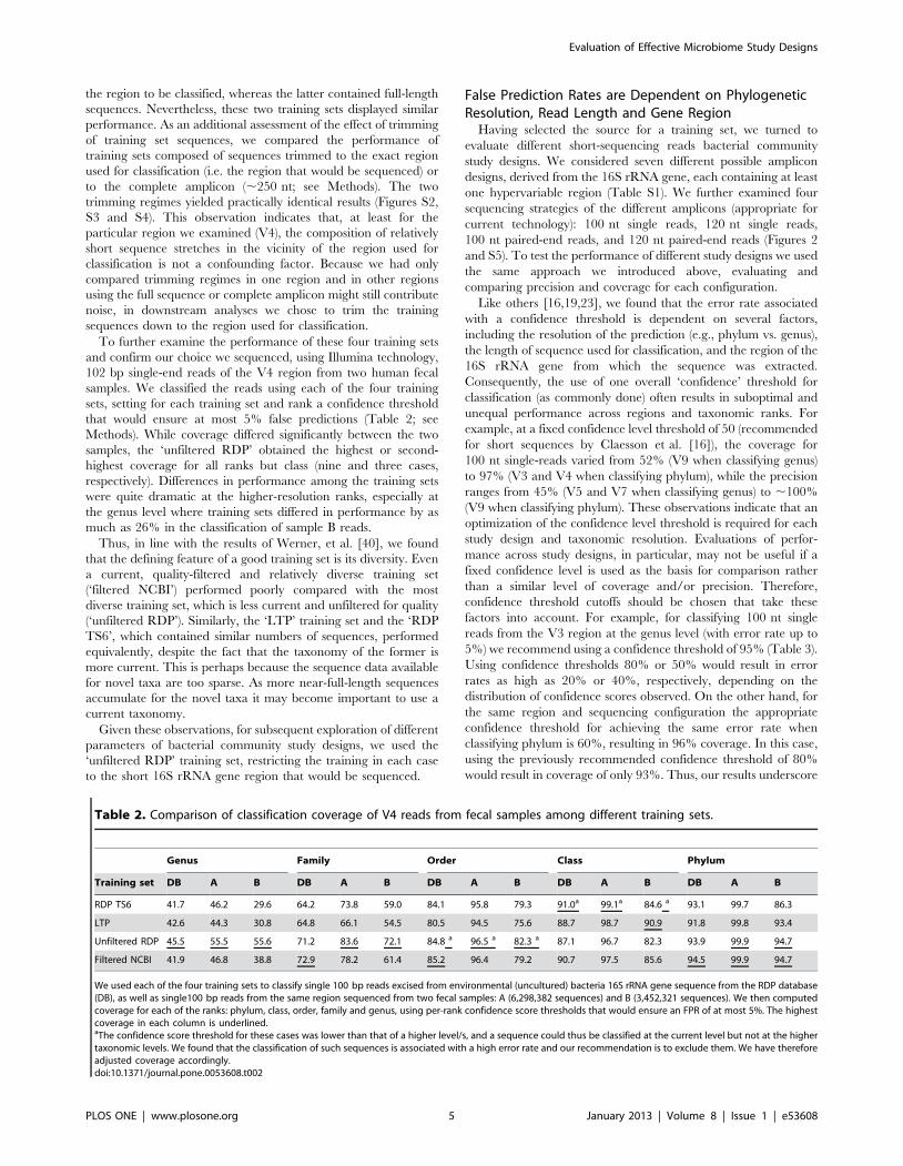
Table 2. Comparison of classification coverage of V4 reads from fecal samples among different training sets.

Genus Family Order Class Phylum

Training set DB A B DB A B DB A B DB A B DB A B

RDP TS6 41.7 46.2 29.6 64.2 73.8 59.0 84.1 95.8 79.3 91.0a 99.1a 84.6 a 93.1 99.7 86.3

LTP 42.6 44.3 30.8 64.8 66.1 54.5 80.5 94.5 75.6 88.7 98.7 90.9 91.8 99.8 93.4

Unfiltered RDP 45.5 55.5 55.6 71.2 83.6 72.1 84.8 a 96.5 a 82.3 a 87.1 96.7 82.3 93.9 99.9 94.7

Filtered NCBI 41.9 46.8 38.8 72.9 78.2 61.4 85.2 96.4 79.2 90.7 97.5 85.6 94.5 99.9 94.7

We used each of the four training sets to classify single 100 bp reads excised from environmental (uncultured) bacteria 16S rRNA gene sequence from the RDP database(DB), as well as single100 bp reads from the same region sequenced from two fecal samples: A (6,298,382 sequences) and B (3,452,321 sequences). We then computedcoverage for each of the ranks: phylum, class, order, family and genus, using per-rank confidence score thresholds that would ensure an FPR of at most 5%. The highestcoverage in each column is underlined.aThe confidence score threshold for these cases was lower than that of a higher level/s, and a sequence could thus be classified at the current level but not at the highertaxonomic levels. We found that the classification of such sequences is associated with a high error rate and our recommendation is to exclude them. We have thereforeadjusted coverage accordingly.doi:10.1371/journal.pone.0053608.t002



the need for a rank-specific and region-specific selection of the

confidence threshold, depending on the desired false prediction

rate (FPR). We provide a tabulation of recommended thresholds

and coverage for a representative group of desired FPRs for all

ranks, regions and configurations examined (Tables S4, S5, S6, S7,

S8, S9 and S10).

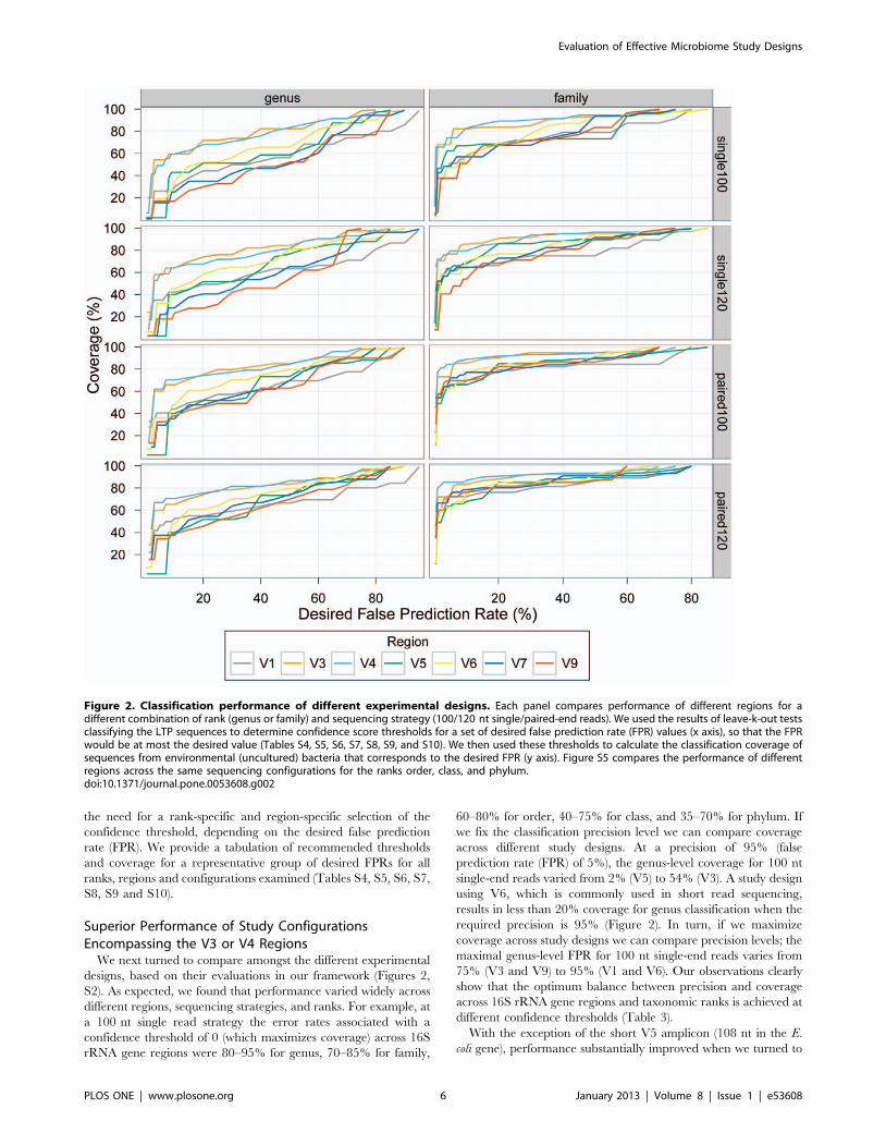
Superior Performance of Study ConfigurationsEncompassing the V3 or V4 Regions

We next turned to compare amongst the different experimental

designs, based on their evaluations in our framework (Figures 2,

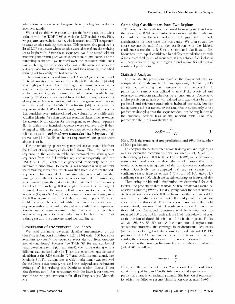
S2). As expected, we found that performance varied widely across

different regions, sequencing strategies, and ranks. For example, at

a 100 nt single read strategy the error rates associated with a

confidence threshold of 0 (which maximizes coverage) across 16S

rRNA gene regions were 80–95% for genus, 70–85% for family,

60–80% for order, 40–75% for class, and 35–70% for phylum. If

we fix the classification precision level we can compare coverage

across different study designs. At a precision of 95% (false

prediction rate (FPR) of 5%), the genus-level coverage for 100 nt

single-end reads varied from 2% (V5) to 54% (V3). A study design

using V6, which is commonly used in short read sequencing,

results in less than 20% coverage for genus classification when the

required precision is 95% (Figure 2). In turn, if we maximize

coverage across study designs we can compare precision levels; the

maximal genus-level FPR for 100 nt single-end reads varies from

75% (V3 and V9) to 95% (V1 and V6). Our observations clearly

show that the optimum balance between precision and coverage

across 16S rRNA gene regions and taxonomic ranks is achieved at

different confidence thresholds (Table 3).

With the exception of the short V5 amplicon (108 nt in the E.

coli gene), performance substantially improved when we turned to

Figure 2. Classification performance of different experimental designs. Each panel compares performance of different regions for adifferent combination of rank (genus or family) and sequencing strategy (100/120 nt single/paired-end reads). We used the results of leave-k-out testsclassifying the LTP sequences to determine confidence score thresholds for a set of desired false prediction rate (FPR) values (x axis), so that the FPRwould be at most the desired value (Tables S4, S5, S6, S7, S8, S9, and S10). We then used these thresholds to calculate the classification coverage ofsequences from environmental (uncultured) bacteria that corresponds to the desired FPR (y axis). Figure S5 compares the performance of differentregions across the same sequencing configurations for the ranks order, class, and phylum.doi:10.1371/journal.pone.0053608.g002



consider study designs with longer sequencing strategies. Exclud-

ing V5, genus-level coverage obtained for 120 nt paired-end reads

(at FPR = 5%) ranged from 34% (V9) to 67% (V4). Differences in

performance between designs using different regions diminished

with decreasing taxonomic resolution. For example, with 100 nt

paired-end reads, the coverage at FPR #5% was 3%–62%, 63%–

84%, 75%–93%, 88%–96%, and 93%–98%, for ranks genus,

family, order, class, and phylum, respectively. Put together, our

analysis suggests that the most effective study design utilizes paired

end sequencing of V3 or V4 amplicons (Figure 2). In addition,

consistent with previous reports [16,19], we found that the V6

region, the region of focus in most bacterial community studies

using short-read sequencing to date [5,6,28,30,39], does not

perform well when a naıve Bayesian classifier approach is used,

especially for classifying high-resolution taxonomic ranks. In

contrast, using the GAST classifier, Huse, et al. [18] found both

the V3 and V6 regions to have similar performance (no other

regions were compared).

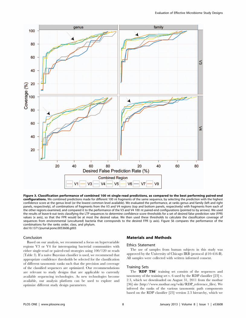
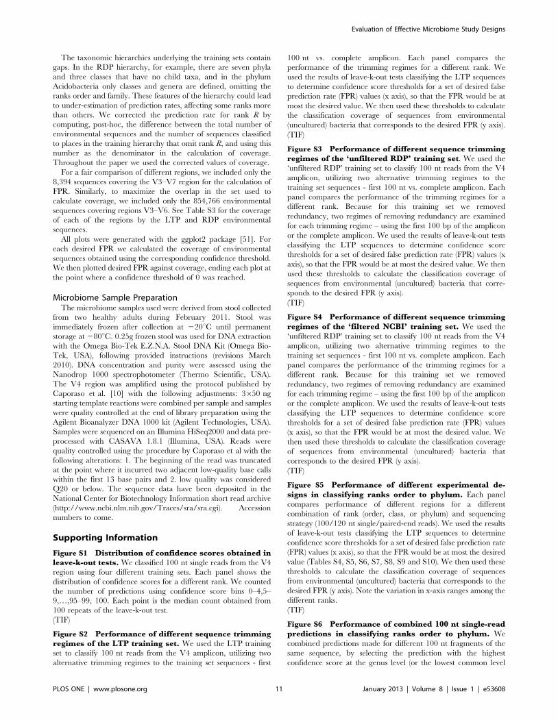
Finally, to extend our analysis to study designs that might be

practical in the near future, we asked if we could improve

performance, whilst sequencing the same number of bases, by

combining single-end reads across amplicons of different hyper-

variable regions instead of using a paired-end sequencing

configuration. To this end we combined the predictions obtained

using 100 nt single reads from each of the best performing regions

(V4 and V3) with those obtained using each of the other

hypervariable regions. We selected for each test sequence the

prediction with highest confidence score at the genus level, with

the assumption that it was known that the two predictions result

from fragments of the same molecule (see Methods for more

details). This is an idealized scenario, not attainable using current

sequencing technologies. Regardless, combined predictions across

multiple regions did not result in an overall improvement

compared to study designs using 100 nt paired-end configurations

of V3 or V4 (Figures 3 and S6).

Our analysis suggests that studies will do equally well focusing

on either V3 or V4, irrespective of whether they choose a single or

paired-end sequencing strategy. Yet, it should be noted that

Youssef, et al. [45] reported that while species-richness estimates

based on V4 are comparable to those from nearly full-length 16S

rRNA gene sequences, analyses of V3 sequences tended to

underestimate species richness. Regardless, the most effective

experimental designs based on our analysis utilize the V3 or V4

paired-end sequence configuration. These designs are more

effective even compared to the paired-end sequence configuration

that overlaps both V7 and V9, and are comparable or more

effective than all the configurations that combined single-read

predictions of the V3/V4 regions with those from each of the

other 16S rRNA gene regions (see Methods and Figures 3 and S6).

Partly, this observation may be explained by the high coverage of

V3 and V4 in the training set. Because not all 16S rRNA gene

reference sequences in the training set are of full length, some

regions of the molecule represent higher diversity than others. For

example, V9 is the region with the least coverage in our database

of reference sequences and correspondingly, study designs using

the V9 regions performed poorly.

In our in silico study we made the unrealistic assumption that the

sequences to be classified contained no errors and thus our results

should be considered best-case scenarios. A good filtration

protocol applied to the reads prior to classification, as well as

filtering results based on their frequency of appearance, may

substantially reduce the effect of sequencing errors in real data

[10,25,27]. Yet, it is important to note that filtering paired-end

reads is likely to result in the removal of a higher number of pairs

compared to filtering single end reads. For that reason, the

advantage we found for the paired-end sequencing strategy should

be considered best-case scenario (see Werner et al., [29] for a

detailed analysis).

In addition, it should be remembered that we assumed an ideal

experimental system in which all primers are universal to bacteria

with no bias. Before any of the primers examined in our study are

utilized in an experimental setting care should be taken that they

are appropriate for the probed environment. That said, the primer

pair used here for the amplification of the V4 region (F515+R806)

has been optimized for broad coverage [46], such that it is nearly

universal.

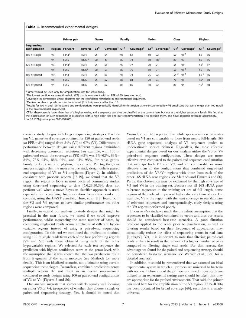
Table 3. Recommended experimental designs.

Primer pair Genus Family Order Class Phylum

Sequencingconfiguration Region Forward Reverse CTb Coveragec CTb Coveragec CTb Coveragec CTb Coveragec CTb Coveragec

100 nt single V3 F343a R534 95 54 95 68 60 92 50 95 f 60 96

V4 F515 R806 a 90 49 80 74 60 88 f 80 90 65 95

120 nt single V3 F343a R534 95 58 90 77 70 91 55 95 50d 97

V4 F515 R806a 90 59 80 79 60 91 50 95 f 55 96

100 nt paired V3e F343 R534 95 60 95 73 75 92 55 d 96 f 60 d 96

V4 F515 R806 95 62 85 84 70 93 70 95 45d 98

120 nt paired V4 F515 R806 95 67 85 85 80 92 80 94 45d 98

aPrimer would be used only for amplification, not for sequencing.bThe lowest confidence value threshold (CT) that is consistent with an FPR of 5% (see methods).cCoverage (in percentage units) observed for the confidence threshold in environmental sequences.dMedian number of predictions in the interval [CT.CT+4] was smaller than 10.eResults for 100 nt and 120 nt paired end configurations were practically identical for this region, as we encountered few V3 amplicons that were longer than 100 nt (allin the environmental sequences).fCT for these cases is lower than that of a higher level/s, and a sequence can thus be classified at the current level but not at the higher taxonomic levels. We find thatthe classification of such sequences is associated with a high error rate and our recommendation is to exclude them, and have adjusted coverage accordingly.doi:10.1371/journal.pone.0053608.t003



ConclusionBased on our analysis, we recommend a focus on hypervariable

regions V3 or V4 for interrogating bacterial communities with

either single-read or paired-end strategies using 100/120 nt reads

(Table 3). If a naıve Bayesian classifier is used, we recommend that

appropriate confidence thresholds be selected for the classification

of different taxonomic ranks such that the precision and coverage

of the classified sequences are optimized. Our recommendations

are relevant to study designs that are applicable to currently

available sequencing technologies. As new technologies become

available, our analysis platform can be used to explore and

optimize different study design parameters.

Materials and Methods

Ethics StatementThe use of samples from human subjects in this study was

approved by the University of Chicago IRB (protocol #10-416-B).

All samples were collected with written informed consent.

Training SetsThe ‘RDP TS6’ training set consists of the sequences and

taxonomy of the training set v. 6 used by the RDP classifier [23] v.

2.3, which we downloaded on August 31, 2011 from the mothur

[36] site (http://www.mothur.org/wiki/RDP_reference_files). We

inferred the ranks of the various taxonomic path components

based on the RDP classifier [23] version 2.3 hierarchy, which we

Figure 3. Classification performance of combined 100 nt single-read predictions, as compared to the best performing paired-endconfigurations. We combined predictions made for different 100 nt fragments of the same sequence, by selecting the prediction with the highestconfidence score at the genus level (or the lowest common level available). We evaluated the performance, at ranks genus and family (left and rightpanels, respectively), of combinations of fragments from the V3 and V4 regions (top and bottom panels, respectively) with fragments from each ofthe other regions examined, and compared it to the performance of the V3 and V4 100 nt paired-end configurations (pointed to by arrows). We usedthe results of leave-k-out tests classifying the LTP sequences to determine confidence score thresholds for a set of desired false prediction rate (FPR)values (x axis), so that the FPR would be at most the desired value. We then used these thresholds to calculate the classification coverage ofsequences from environmental (uncultured) bacteria that corresponds to the desired FPR (y axis). Figure S6 compares the performance of thecombinations for the ranks order, class, and phylum.doi:10.1371/journal.pone.0053608.g003



downloaded from http://sourceforge.net/projects/rdp-classifier.

To determine the species classification corresponding to the

sequences, we used the annotation in the headers of the sequences

of the SSURef subset of Release 108 of the SILVA database [47],

downloaded from http://www.arb-silva.de/no_cache/download/

archive/release_108/Exports/on September 1, 2011. For the few

training sequences missing from the SSURef dataset, we obtained

the species name manually from the NCBI website [48].

The ‘unfiltered RDP’ and ‘filtered NCBI’ training sets are

based on bacterial isolate sequences from the RDP database

[43,44]. We used the RDP browser (http://rdp.cme.msu.edu/

hierarchy/hb_intro.jsp) to download, on February 25, 2011,

sequence alignment and annotation data for 250,706 high quality

16S rRNA sequences amplified from bacterial isolates, utilizing the

nomenclatural taxonomy.

We obtained the taxonomic annotation of the ‘unfilteredRDP’ training set from the RDP database [43,44] records, relying

on the RDP classifier hierarchy for inference of the rank of

taxonomic path components. In some cases, we found that the

same name is given to different levels of the hierarchy (e.g.

‘‘Actinobacteria’’ is both the name of a phylum and a class). To

obtain the rank in these cases we relied on the parent-child

relationships specified by the hierarchy and the order of names in

the taxonomic path. We used the Bio::LITE::Taxonomy::NCBI

module version 0.06 to extract the species name corresponding to

the NCBI taxonomic identifier in the sequence record from a local

copy of the NCBI taxonomy database [48], which we downloaded

from ftp://ftp.ncbi.nih.gov/pub/taxonomy/on March 2, 2011.

See Methods S1 for additional details on the inferred taxonomic

annotation of this training set.

For the ‘filtered NCBI’ training set we inferred the taxonomic

classification, including species, using the NCBI taxonomic

identifier in the sequence record and the local copy of the NCBI

taxonomy database [48], utilizing Bio::LITE::Taxonomy::NCBI

version 0.06. We removed from this dataset any sequence for

which phylum or genus annotation was missing. We then

performed additional filtering retaining only sequences whose

classification in NCBI was consistent with their RDP annotation

for phylum, class, order, family and genus or if the sequence

classification contains a value unique to NCBI where there is

disagreement between the databases (because this likely represents

a recent addition to the taxonomic hierarchy). While performing

this filtration we found systematic differences between the NCBI

and RDP hierarchies. We added the sequences conforming with

the filtration criteria after accounting for these systematic

differences to the final training set. Finally, the ‘LTP’ training

set consists of the bacterial sequences and taxonomic annotation

from ‘‘The All-Species Living Tree" project (LTP) [41,42]. We

downloaded LTP release 106 annotation data and multiple

sequence alignment from http://www.arb-silva.de/projects/

living-tree/) on August 30, 2011. We used the ‘‘tax_ltp’’ field for

taxonomic annotation down to the genus level, excluding

annotations where the rank was specified as ‘Unclassified’. We

obtained species names from the ‘‘fullname_ltp’’ field, removing

subspecies information where present.

To facilitate the extraction of rank information from predicted

taxonomic paths, we prefixed each taxon name within the training

taxonomies with the corresponding rank. We also excluded

taxonomic path components that began with ‘‘unclassified’’ or

ended with ‘‘incertae_sedis’’.

We tested the performance of different training sets by

classifying sequences of simulated amplicons surrounding the V4

hypervariable region, which has been widely used for high-

throughput 16S rRNA gene sequencing [10]. We focused on the

100 nt single-end sequencing strategy (namely, the first 100 bp of

the amplicon), which is the most challenging experimental

configuration among those examined in this work.

Test SetsTo measure precision (or the false prediction rate, which is 1-

[precision]) we used the bacterial sequences and taxonomic

annotation from ‘‘The All-Species Living Tree" project (LTP)

(Munoz, et al., 2011; Yarza, et al., 2008) for leave-k-out testing –

this set is identical to the LTP training set. In turn, to measure

coverage, we used 1,462,503 high quality 16S rRNA gene

sequences amplified from environmental (uncultured) bacteria.

We downloaded these sequences, in MSA format, from the RDP

browser (http://rdp.cme.msu.edu/hierarchy/hb_intro.jsp, (Cole,

et al., 2007; Cole, et al., 2009)) on September 21, 2011.

Extraction of Amplicon SequencesThe basis for our analyses are the sequence reads that would

have been obtained if the primer pairs (Table S1) produced an

amplicon from any bacterial 16S rRNA gene sequence (namely,

with no bias). To simulate this set of reads we started by extracting,

for each primer pair, the subsequences it would amplify (i.e. the

amplicons) from all available sequences that covered this region.

This was performed for the LTP bacterial sequence set, the RDP

bacterial isolates set, and the RDP environmental (uncultured)

bacteria set, using python scripts that utilize Biopython [49]

modules. First, we found the coordinates covered by the two

primers on a reference sequence (Table S2). To avoid missing

insertions that are adjacent to the primers we added one flanking

position on each side of the amplicon. We then extracted the

corresponding sub-alignment, including only sequences that begin

before or at the first column of the sub-alignment and end after or

at its last column. Finally, to obtain the collection of amplicons, we

removed the first and last columns of this sub-alignment and the

gap characters. To ensure the high quality of the RDP [43,44]

sequences included in our training sets we performed length

filtration of the amplicons, which resulted in loss of at most 0.16%

of sequences (see Methods S1).

Generation of Short Read DataTo obtain single reads of length X bases (X = 100 or 120) from

the amplicon data we extracted the first (forward read) or last

(reverse read) X bases from each amplicon sequence. The read

direction used (Table S1) was selected to optimize the number of

hypervariable region bases covered. To obtain paired-end

sequences for reads of length X from the amplicon data we fused

the first and last X bases of the amplicon sequence, separating the

two subsequences by a run of ten N’s. If the amplicon length was

shorter or equal to 2X we used the amplicon sequence. Finally, we

filtered out any sequence ‘reads’ that contained more than ten

ambiguous characters (excluding intervening runs of N’s) from the

‘unfiltered RDP’ and ‘filtered NCBI’ training sets.

Leave k Out Classification TestsWe evaluated the precision expected from each of the training

sets by classifying sequence fragments derived from the bacterial

portion of LTP [41,42] using a leave-k-out approach. To classify a

sequence S we first excluded from the training set all sequences

annotated as derived from the same species. We then classified S,

using the naıve Bayesian classifier implemented by the classify.seqs

function in mothur v.1.20.1 [36] with 1000 bootstrap iterations. In

all cases we trimmed the training taxonomies to contain



information only down to the genus level (the highest resolution

level evaluated).

We used the following procedure for the leave-k-out tests when

training with the ‘RDP TS6’ or with the LTP training sets. First,

we prepared an exclusion table, which related test (LTP) sequences

to same-species training sequences. This process also produced a

list of LTP sequences whose species were absent from the training

set to begin with. Since these sequences could be tested without

modifying the training set we classified them as one batch. For the

remaining sequences, we iterated over the exclusion table, each

time excluding the sequences belonging to the same species as the

test sequence from the training set, and then using this modified

training set to classify the test sequence.

The training sets derived from the 16S rRNA gene sequences of

bacterial isolates downloaded from the RDP database [43,44]

were highly redundant. For tests using these training sets we used a

modified procedure that minimizes the redundancy in sequence,

whilst maximizing the taxonomic information available for

training. To do so, we extracted from the full training set a subset

of sequences that was non-redundant at the genus level. To this

end, we used the USEARCH software [50] to cluster the

sequences at the 100% identity level, using the ‘–iddef 19 option

that considers every mismatch and gap column to be a difference

to define identity. We then used the resulting clusters file, as well as

the taxonomic annotation for the sequences, to obtain sequence

files in which two identical sequences were retained only if they

belonged to different genera. This reduced set will subsequently be

referred to as the ‘original non-redundant training set’. This

set was used for classifying the test sequences whose species were

absent from it.

For the remaining species we generated an exclusion table from

the full set of sequences, as described above. Then, for each test

sequence in the exclusion table, we removed the same-species

sequences from the full training set, and subsequently used the

USEARCH [50] cluster file generated previously with the

taxonomic annotation, to create a non-redundant training set from

the remaining sequences, which was then used to classify the test-

sequence. This avoided the potential elimination of available

same-genus different-species sequences from the training set,

which would make the test stricter than intended. For examining

the effect of classifying 100 nt single-reads with a training set

trimmed down to the same 100 nt region or to the complete

amplicon (Figures S3, S4, S5), we removed redundancy using only

the 100 nt region tested for both the trimming regimes. Thus, we

could focus on the effect of additional bases within the same

sequence without the confounding effects of additional sequences.

Similar results were obtained when we used the complete

amplicon sequence to filter redundancy for both the 100 nt

training set and the complete amplicon training set.

Classification of Environmental SequencesWe used the naıve Bayesian classifier implemented by the

classify.seqs function in mothur v.1.20.1 [36] with 1000 bootstrap

iterations to classify the sequence reads derived from environ-

mental (uncultured) bacteria (see Table S3, for the number of

reads covering each region examined), each time training with a

different training set (Table 1). This classifier implements the same

algorithm as the RDP classifier [23] and performs equivalently (see

Methods S1). For training sets in which redundancy was removed

for the leave-k-out testing, we used the ‘original non-redundant

training set’ for training (see Methods section ‘Leave k out

classification tests’). For consistency with the leave-k-out tests, we

used the rearranged taxonomies for all training sets (see Methods

S1).

Combining Classifications from Two RegionsTo combine the predictions obtained from regions A and B of

the same 16S rRNA gene molecule we examined the prediction

for rank R, the highest resolution rank predicted by both

classifications (in most cases this was genus). We then copied the

entire taxonomic path from the prediction with the highest

confidence score for rank R to the combined classification file.

Sequences with equal confidence but different predictions at rank

R were discarded (,1% of sequences in any dataset). We included

only sequences covering both region A and region B in the set of

combined predictions.

Statistical AnalysesTo evaluate the predictions made in the leave-k-out tests we

compared the prediction to the corresponding reference (LTP)

annotation, evaluating each taxonomic rank separately. A

prediction at rank R was defined as true if the predicted and

reference annotations matched or were synonymous. Conversely,

a false prediction at rank R was defined as a case where both the

predicted and reference annotations included this rank, but the

taxon names did not match, or the rank was included only in the

prediction (implying that the sequence does not belong in any of

the currently defined taxa at the relevant rank). The false

prediction rate (FPR) was defined as.

FPR~FP

TPzFPð1Þ

Here, TP is the number of true predictions, and FP is the number

of false predictions.

To compare the performance across training sets and regions, as

well as formulate recommendations, we used a set, E, of FPR

values ranging from 0.001 to 0.95. For each eME, we determined a

conservative confidence threshold that would ensure that FPR

would be at most e, irrespective of the distribution of confidence

values. Specifically, we computed TP and FP counts over

confidence score intervals of size 5 (0–4, …, 95–99), except for

confidence score 100, which we calculated using an interval of size

1. Then, using the binomial distribution, we determined for each

interval the probability that at most TP true predictions would be

observed assuming FPR = e. Finally, going down the set of intervals

starting at confidence score 100, we looked for the first interval for

which this probability was at most 0.05, and picked the interval

above it as the threshold. Thus, the chosen confidence threshold

conservatively assumes that all confidence scores fall into the

threshold bin. For added robustness, each leave-k-out test was

repeated 100 times and for each eME the final threshold was chosen

as the median of thresholds obtained for e in the repeats. Tables

S4, S5, S6, S7, S8, S9, and S10 contain, for all regions and

sequencing strategies, the coverage in environmental sequences

(see below) including both the cumulative and interval TP, FP,

precision and FPR. For confidence scores that were selected as

cutoffs, the corresponding desired FPR is also indicated.

We define the coverage for rank R and confidence threshold c

(0#c#100) as follows:

coverage ~n

sð2Þ

Here, n is the number of times R is predicted with confidence

greater or equal to c, and S is the total number of sequences with a

prediction at any level, including domain (the fraction of sequences

for which we failed to get any classification was at most 6e-05).



The taxonomic hierarchies underlying the training sets contain

gaps. In the RDP hierarchy, for example, there are seven phyla

and three classes that have no child taxa, and in the phylum

Acidobacteria only classes and genera are defined, omitting the

ranks order and family. These features of the hierarchy could lead

to under-estimation of prediction rates, affecting some ranks more

than others. We corrected the prediction rate for rank R by

computing, post-hoc, the difference between the total number of

environmental sequences and the number of sequences classified

to places in the training hierarchy that omit rank R, and using this

number as the denominator in the calculation of coverage.

Throughout the paper we used the corrected values of coverage.

For a fair comparison of different regions, we included only the

8,394 sequences covering the V3–V7 region for the calculation of

FPR. Similarly, to maximize the overlap in the set used to

calculate coverage, we included only the 854,766 environmental

sequences covering regions V3–V6. See Table S3 for the coverage

of each of the regions by the LTP and RDP environmental

sequences.

All plots were generated with the ggplot2 package [51]. For

each desired FPR we calculated the coverage of environmental

sequences obtained using the corresponding confidence threshold.

We then plotted desired FPR against coverage, ending each plot at

the point where a confidence threshold of 0 was reached.

Microbiome Sample PreparationThe microbiome samples used were derived from stool collected

from two healthy adults during February 2011. Stool was

immediately frozen after collection at 220uC until permanent

storage at 280uC. 0.25g frozen stool was used for DNA extraction

with the Omega Bio-Tek E.Z.N.A. Stool DNA Kit (Omega Bio-

Tek, USA), following provided instructions (revisions March

2010). DNA concentration and purity were assessed using the

Nanodrop 1000 spectrophotometer (Thermo Scientific, USA).

The V4 region was amplified using the protocol published by

Caporaso et al. [10] with the following adjustments: 3650 ng

starting template reactions were combined per sample and samples

were quality controlled at the end of library preparation using the

Agilent Bioanalyzer DNA 1000 kit (Agilent Technologies, USA).

Samples were sequenced on an Illumina HiSeq2000 and data pre-

processed with CASAVA 1.8.1 (Illumina, USA). Reads were

quality controlled using the procedure by Caporaso et al with the

following alterations: 1. The beginning of the read was truncated

at the point where it incurred two adjacent low-quality base calls

within the first 13 base pairs and 2. low quality was considered

Q20 or below. The sequence data have been deposited in the

National Center for Biotechnology Information short read archive

(http://www.ncbi.nlm.nih.gov/Traces/sra/sra.cgi). Accession

numbers to come.

Supporting Information

Figure S1 Distribution of confidence scores obtained inleave-k-out tests. We classified 100 nt single reads from the V4

region using four different training sets. Each panel shows the

distribution of confidence scores for a different rank. We counted

the number of predictions using confidence score bins 0–4,5–

9,…,95–99, 100. Each point is the median count obtained from

100 repeats of the leave-k-out test.

(TIF)

Figure S2 Performance of different sequence trimmingregimes of the LTP training set. We used the LTP training

set to classify 100 nt reads from the V4 amplicon, utilizing two

alternative trimming regimes to the training set sequences - first

100 nt vs. complete amplicon. Each panel compares the

performance of the trimming regimes for a different rank. We

used the results of leave-k-out tests classifying the LTP sequences

to determine confidence score thresholds for a set of desired false

prediction rate (FPR) values (x axis), so that the FPR would be at

most the desired value. We then used these thresholds to calculate

the classification coverage of sequences from environmental

(uncultured) bacteria that corresponds to the desired FPR (y axis).

(TIF)

Figure S3 Performance of different sequence trimmingregimes of the ‘unfiltered RDP’ training set. We used the

‘unfiltered RDP’ training set to classify 100 nt reads from the V4

amplicon, utilizing two alternative trimming regimes to the

training set sequences - first 100 nt vs. complete amplicon. Each

panel compares the performance of the trimming regimes for a

different rank. Because for this training set we removed

redundancy, two regimes of removing redundancy are examined

for each trimming regime – using the first 100 bp of the amplicon

or the complete amplicon. We used the results of leave-k-out tests

classifying the LTP sequences to determine confidence score

thresholds for a set of desired false prediction rate (FPR) values (x

axis), so that the FPR would be at most the desired value. We then

used these thresholds to calculate the classification coverage of

sequences from environmental (uncultured) bacteria that corre-

sponds to the desired FPR (y axis).

(TIF)

Figure S4 Performance of different sequence trimmingregimes of the ‘filtered NCBI’ training set. We used the

‘unfiltered RDP’ training set to classify 100 nt reads from the V4

amplicon, utilizing two alternative trimming regimes to the

training set sequences - first 100 nt vs. complete amplicon. Each

panel compares the performance of the trimming regimes for a

different rank. Because for this training set we removed

redundancy, two regimes of removing redundancy are examined

for each trimming regime – using the first 100 bp of the amplicon

or the complete amplicon. We used the results of leave-k-out tests

classifying the LTP sequences to determine confidence score

thresholds for a set of desired false prediction rate (FPR) values

(x axis), so that the FPR would be at most the desired value. We

then used these thresholds to calculate the classification coverage

of sequences from environmental (uncultured) bacteria that

corresponds to the desired FPR (y axis).

(TIF)

Figure S5 Performance of different experimental de-signs in classifying ranks order to phylum. Each panel

compares performance of different regions for a different

combination of rank (order, class, or phylum) and sequencing

strategy (100/120 nt single/paired-end reads). We used the results

of leave-k-out tests classifying the LTP sequences to determine

confidence score thresholds for a set of desired false prediction rate

(FPR) values (x axis), so that the FPR would be at most the desired

value (Tables S4, S5, S6, S7, S8, S9 and S10). We then used these

thresholds to calculate the classification coverage of sequences

from environmental (uncultured) bacteria that corresponds to the

desired FPR (y axis). Note the variation in x-axis ranges among the

different ranks.

(TIF)

Figure S6 Performance of combined 100 nt single-readpredictions in classifying ranks order to phylum. We

combined predictions made for different 100 nt fragments of the

same sequence, by selecting the prediction with the highest

confidence score at the genus level (or the lowest common level



available). We evaluated the performance of combinations of

fragments from the V3 and V4 regions (top and bottom panels,

respectively) with fragments from each of the other regions

examined, and compared it to the performance of the V3 (orange

curve in top panels) and V4 (light blue curve in bottom panels)

100 nt paired-end configurations. We used the results of leave-k-

out tests classifying the LTP sequences to determine confidence

score thresholds for a set of desired false prediction rate (FPR)

values (x axis), so that the FPR would be at most the desired value.

We then used these thresholds to calculate the classification

coverage of sequences from environmental (uncultured) bacteria

that corresponds to the desired FPR (y axis). Note the variation in

x-axis ranges among the different ranks.

(TIF)

Table S1 Primer pairs studied. The sequences of the

primers in each pair, the read direction used for single-read

sequencing, and the hypervariable region/s of the 16S rRNA gene

covered using the sequencing strategies studied in this work are

indicated.

(DOC)

Table S2 Coordinates of the amplicons studied on thereference sequences used: RDP database bacterial isolates –

S000495522 (GenBank AB035921); LTP – X80725 (*) and

AJ508775 (**); RDP uncultured bacteria – S001235409 (Genbank

FJ479556).

(DOC)

Table S3 Coverage of the examined amplicons by LTPand RDP uncultured bacterial sequences. We identify each

amplicon using the 16S rRNA gene hypervariable region covered

by single-read sequencing configurations. We counted sequences

only if they contained the entire amplicon.

(DOC)

Table S4 Summary of analyses for V1. For each sequenc-

ing configuration, taxonomic rank and bootstrap confidence value

C, we provide the following information pertaining to the interval

[C.C+4] (except for the case C = 100, in which the interval is of

size 1): Interval_TP - median number of true predictions in leave-

k-out tests (out of 100 repeats); Interval_FP - median number of

false predictions in leave-k-out tests (out of 100 repeats);

Interval_precision - precision in leave-k-out tests (%), calculated

from Interval_TP and Interval_FP; Interval_FPR - false prediction

rate in leave-k-out tests (%), calculated from Interval_TP and

Interval_FP; threshold for FPR – FPR values for which the

confidence value is suitable as a threshold (note that not all rows

will contain this field, as we tested only a limited set of FPR values),

each threshold is the median of 100 thresholds obtained for the

same desired FPR from 100 repeats of the leave-k-out test. We also

provide the following information for the interval [C.100]:

Env_coverage - coverage of environmental sequences (%);

Cumulative_TP - number of true predictions in leave-k-out tests,

calculated from Interval_TP; Cumulative_FP - number of false

predictions in leave-k-out tests, calculated from Interval_FP;

Cumulative_precision – precision of leave-k-out tests (%),

calculated from Cumulative_TP and Cumulative_FP; Cumulati-

ve_FPR – false prediction rate of leave-k-out tests (%), calculated

from Cumulative_TP and Cumulative_FP.

(XLS)

























(XLS)

























(XLS)



























(XLS)

























(XLS)

























(XLS)

Table S10 Summary of analyses for V9. For each

sequencing configuration, taxonomic rank and bootstrap confi-

dence value C, we provide the following information pertaining to

the interval [C.C+4] (except for the case C = 100, in which the

interval is of size 1): Interval_TP - median number of true

predictions in leave-k-out tests (out of 100 repeats); Interval_FP -

median number of false predictions in leave-k-out tests (out of 100

repeats); Interval_precision - precision in leave-k-out tests (%),

calculated from Interval_TP and Interval_FP; Interval_FPR - false

prediction rate in leave-k-out tests (%), calculated from Inter-

val_TP and Interval_FP; threshold for FPR – FPR values for

which the confidence value is suitable as a threshold (note that not

all rows will contain this field, as we tested only a limited set of

FPR values), each threshold is the median of 100 thresholds

obtained for the same desired FPR from 100 repeats of the leave-

k-out test. We also provide the following information for the

interval [C.100]: Env_coverage - coverage of environmental

sequences (%); Cumulative_TP - number of true predictions in

leave-k-out tests, calculated from Interval_TP; Cumulative_FP -

number of false predictions in leave-k-out tests, calculated from

Interval_FP; Cumulative_precision – precision of leave-k-out tests

(%), calculated from Cumulative_TP and Cumulative_FP; Cu-

mulative_FPR – false prediction rate of leave-k-out tests (%),

calculated from Cumulative_TP and Cumulative_FP.

(XLS)

Methods S1

(DOC)

Acknowledgments

We thank members of the Gilad lab for helpful discussions and C. Ober

and Z. Gauhar for comments on the manuscript. This work was supported

by NIH grant HL092206 to YG, and by a pilot and feasibility DDRCC

grant to YG, funded by P30DK42086.

Author Contributions

Conceived and designed the experiments: YG OM ED. Performed the

experiments: OM ED. Analyzed the data: OM ED. Contributed reagents/

materials/analysis tools: YG. Wrote the paper: OM ED YG.

References

1. Pace NR (1997) A molecular view of microbial diversity and the biosphere.

Science 276: 734–740.

2. Woese CR, Fox GE (1977) Phylogenetic structure of the prokaryotic domain: the

primary kingdoms. Proc Natl Acad Sci U S A 74: 5088–5090.

3. Arumugam M, Raes J, Pelletier E, Le Paslier D, Yamada T, et al. (2011)

Enterotypes of the human gut microbiome. Nature 473: 174–180.

4. Costello EK, Lauber CL, Hamady M, Fierer N, Gordon JI, et al. (2009)

Bacterial community variation in human body habitats across space and time.

Science 326: 1694–1697.

5. Turnbaugh PJ, Hamady M, Yatsunenko T, Cantarel BL, Duncan A, et al.

(2009) A core gut microbiome in obese and lean twins. Nature 457: 480–484.

6. Gilbert JA, Field D, Swift P, Newbold L, Oliver A, et al. (2009) The seasonal

structure of microbial communities in the Western English Channel. Environ

Microbiol 11: 3132–3139.

7. Hackl E, Zechmeister-Boltenstern S, Bodrossy L, Sessitsch A (2004) Comparison

of diversities and compositions of bacterial populations inhabiting natural forest

soils. Appl Environ Microbiol 70: 5057–5065.

8. Woese CR (1987) Bacterial evolution. Microbiol Rev 51: 221–271.

9. Clarridge JE (2004) Impact of 16S rRNA gene sequence analysis for

identification of bacteria on clinical microbiology and infectious diseases. Clin

Microbiol Rev 17: 840–862, table of contents.

10. Caporaso JG, Lauber CL, Walters WA, Berg-Lyons D, Lozupone CA, et al.

(2011) Global patterns of 16S rRNA diversity at a depth of millions of sequences

per sample. Proc Natl Acad Sci U S A 108 Suppl 1: 4516–4522.

11. Claesson MJ, Wang Q, O’Sullivan O, Greene-Diniz R, Cole JR, et al. (2010)

Comparison of two next-generation sequencing technologies for resolving highly

complex microbiota composition using tandem variable 16S rRNA gene regions.

Nucleic Acids Res 38: e200.

12. Tringe SG, Hugenholtz P (2008) A renaissance for the pioneering 16S rRNA

gene. Curr Opin Microbiol 11: 442–446.



13. Hummelen R, Fernandes AD, Macklaim JM, Dickson RJ, Changalucha J, et al.

(2010) Deep sequencing of the vaginal microbiota of women with HIV. PLoSOne 5: e12078.

14. Lazarevic V, Whiteson K, Huse S, Hernandez D, Farinelli L, et al. (2009)

Metagenomic study of the oral microbiota by Illumina high-throughputsequencing. J Microbiol Methods 79: 266–271.

15. Yatsunenko T, Rey FE, Manary MJ, Trehan I, Dominguez-Bello MG, et al.(2012) Human gut microbiome viewed across age and geography. Nature 486:

222–227.

16. Claesson MJ, O’Sullivan O, Wang Q, Nikkila J, Marchesi JR, et al. (2009)Comparative analysis of pyrosequencing and a phylogenetic microarray for

exploring microbial community structures in the human distal intestine. PLoSOne 4: e6669.

17. Hamady M, Knight R (2009) Microbial community profiling for humanmicrobiome projects: Tools, techniques, and challenges. Genome Res 19: 1141–

1152.

18. Huse SM, Dethlefsen L, Huber JA, Mark Welch D, Welch DM, et al. (2008)Exploring microbial diversity and taxonomy using SSU rRNA hypervariable tag

sequencing. PLoS Genet 4: e1000255.19. Liu Z, DeSantis TZ, Andersen GL, Knight R (2008) Accurate taxonomy

assignments from 16S rRNA sequences produced by highly parallel pyrose-

quencers. Nucleic Acids Res 36: e120.20. Nossa CW, Oberdorf WE, Yang L, Aas JA, Paster BJ, et al. (2010) Design of 16S

rRNA gene primers for 454 pyrosequencing of the human foregut microbiome.World J Gastroenterol 16: 4135–4144.

21. Soergel DAW, Dey N, Knight R, Brenner SE (2012) Selection of primers foroptimal taxonomic classification of environmental 16S rRNA gene sequences.

ISME J.

22. Sundquist A, Bigdeli S, Jalili R, Druzin ML, Waller S, et al. (2007) Bacterialflora-typing with targeted, chip-based Pyrosequencing. BMC Microbiol 7: 108.

23. Wang Q, Garrity GM, Tiedje JM, Cole JR (2007) Naive Bayesian classifier forrapid assignment of rRNA sequences into the new bacterial taxonomy. Appl

Environ Microbiol 73: 5261–5267.

24. Bartram AK, Lynch MD, Stearns JC, Moreno-Hagelsieb G, Neufeld JD (2011)Generation of multimillion-sequence 16S rRNA gene libraries from complex

microbial communities by assembling paired-end illumina reads. Appl EnvironMicrobiol 77: 3846–3852.

25. Degnan PH, Ochman H (2012) Illumina-based analysis of microbial communitydiversity. ISME J 6: 183–194.

26. Fagen JR, Giongo A, Brown CT, Davis-Richardson AG, Gano KA, et al. (2012)

Characterization of the Relative Abundance of the Citrus Pathogen Ca.Liberibacter Asiaticus in the Microbiome of Its Insect Vector, Diaphorina citri,

using High Throughput 16S rRNA Sequencing. Open Microbiol J 6: 29–33.27. Gloor GB, Hummelen R, Macklaim JM, Dickson RJ, Fernandes AD, et al.

(2010) Microbiome profiling by illumina sequencing of combinatorial sequence-

tagged PCR products. PLoS One 5: e15406.28. Hummelen R, Macklaim JM, Bisanz JE, Hammond J-A, McMillan A, et al.

(2011) Vaginal microbiome and epithelial gene array in post-menopausalwomen with moderate to severe dryness. PLoS One 6: e26602.

29. Werner JJ, Zhou D, Caporaso JG, Knight R, Angenent LT (2012) Comparisonof Illumina paired-end and single-direction sequencing for microbial 16S rRNA

gene amplicon surveys. ISME J 6: 1273–1276.

30. Finkel OM, Burch AY, Lindow SE, Post AF, Belkin S (2011) Geographicallocation determines the population structure in phyllosphere microbial

communities of a salt-excreting desert tree. Appl Environ Microbiol 77: 7647–7655.

31. Shepherd ML, Swecker WS, Jensen RV, Ponder MA (2012) Characterization of

the fecal bacteria communities of forage-fed horses by pyrosequencing of 16SrRNA V4 gene amplicons. FEMS Microbiol Lett 326: 62–68.

32. Wang T, Cai G, Qiu Y, Fei N, Zhang M, et al. (2012) Structural segregation ofgut microbiota between colorectal cancer patients and healthy volunteers.

ISME J 6: 320–329.

33. Zhang X, Yue S, Zhong H, Hua W, Chen R, et al. (2011) A diverse bacterialcommunity in an anoxic quinoline-degrading bioreactor determined by using

pyrosequencing and clone library analysis. Appl Microbiol Biotechnol 91: 425–

434.

34. Matsen FA, Kodner RB, Armbrust EV (2010) pplacer: linear time maximum-

likelihood and Bayesian phylogenetic placement of sequences onto a fixed

reference tree. BMC Bioinformatics 11: 538.

35. DeSantis TZ, Keller K, Karaoz U, Alekseyenko AV, Singh NN, et al. (2011)

Simrank: Rapid and sensitive general-purpose k-mer search tool. BMC Ecol 11:

11.

36. Schloss PD, Westcott SL, Ryabin T, Hall JR, Hartmann M, et al. (2009)

Introducing mothur: open-source, platform-independent, community-supported

software for describing and comparing microbial communities. Appl EnvironMicrobiol 75: 7537–7541.

37. Charlson ES, Bittinger K, Chen J, Diamond JM, Li H, et al. (2012) Assessing

bacterial populations in the lung by replicate analysis of samples from the upperand lower respiratory tracts. PLoS One 7: e42786.

38. Kohler T, Dietrich C, Scheffrahn RH, Brune A (2012) High-resolution analysis

of gut environment and bacterial microbiota reveals functional compartmenta-tion of the gut in wood-feeding higher termites (Nasutitermes spp.). Appl

Environ Microbiol 78: 4691–4701.

39. Nakayama J, Kobayashi T, Tanaka S, Korenori Y, Tateyama A, et al. (2011)Aberrant structures of fecal bacterial community in allergic infants profiled by

16S rRNA gene pyrosequencing. FEMS Immunol Med Microbiol 63: 397–406.

40. Werner JJ, Koren O, Hugenholtz P, DeSantis TZ, Walters WA, et al. (2012)

Impact of training sets on classification of high-throughput bacterial 16s rRNA

gene surveys. ISME J 6: 94–103.

41. Munoz R, Yarza P, Ludwig W, Euzeby J, Amann R, et al. (2011) Release

LTPs104 of the All-Species Living Tree. Syst Appl Microbiol 34: 169–170.

42. Yarza P, Richter M, Peplies J, Euzeby J, Amann R, et al. (2008) The All-SpeciesLiving Tree project: a 16S rRNA-based phylogenetic tree of all sequenced type

strains. Syst Appl Microbiol 31: 241–250.

43. Cole JR, Chai B, Farris RJ, Wang Q, Kulam-Syed-Mohideen AS, et al. (2007)The ribosomal database project (RDP-II): introducing myRDP space and

quality controlled public data. Nucleic Acids Res 35: D169–172.

44. Cole JR, Wang Q, Cardenas E, Fish J, Chai B, et al. (2009) The RibosomalDatabase Project: improved alignments and new tools for rRNA analysis.

Nucleic Acids Res 37: D141–145.

45. Youssef N, Sheik CS, Krumholz LR, Najar FZ, Roe BA, et al. (2009)Comparison of species richness estimates obtained using nearly complete

fragments and simulated pyrosequencing-generated fragments in 16S rRNA

gene-based environmental surveys. Appl Environ Microbiol 75: 5227–5236.

46. Walters WA, Caporaso JG, Lauber CL, Berg-Lyons D, Fierer N, et al. (2011)

PrimerProspector: de novo design and taxonomic analysis of barcoded

polymerase chain reaction primers. Bioinformatics 27: 1159–1161.

47. Pruesse E, Quast C, Knittel K, Fuchs BM, Ludwig W, et al. (2007) SILVA: a

comprehensive online resource for quality checked and aligned ribosomal RNAsequence data compatible with ARB. Nucleic Acids Res 35: 7188–7196.

48. Sayers EW, Barrett T, Benson DA, Bolton E, Bryant SH, et al. (2011) Database

resources of the National Center for Biotechnology Information. Nucleic AcidsRes 39: D38–51.

49. Cock PJA, Antao T, Chang JT, Chapman BA, Cox CJ, et al. (2009) Biopython:

freely available Python tools for computational molecular biology andbioinformatics. Bioinformatics 25: 1422–1423.

50. Edgar RC (2010) Search and clustering orders of magnitude faster than BLAST.

Bioinformatics 26: 2460–2461.

51. Wickham H (2009) ggplot2: elegant graphics for data analysis: Springer New

York.

52. Garrity GM, Lilburn TG, Cole JR, Harrison SH, Euzeby J, et al. (2007) TheTaxonomic Outline of Bacteria and Archaea. TOBA Release 7.7. MI, USA:

Michigan State University Board of Trustees.



Taxonomic Classification of Bacterial 16S rRNA Genes Using ...

Documents