DISCUSSION PAPER SERIES IN ECONOMICS AND MANAGEMENT Tax and Managerial Effects of Transfer Pricing on Capital and Physical Products Oliver Duerr, Thomas Rüffieux Discussion Paper No. 17-19 GERMAN ECONOMIC ASSOCIATION OF BUSINESS ADMINISTRATION – GEABA

Welcome message from author
This document is posted to help you gain knowledge. Please leave a comment to let me know what you think about it! Share it to your friends and learn new things together.
Transcript

DISCUSSION PAPER SERIES IN ECONOMICS AND MANAGEMENT
Tax and Managerial Effects of Transfer Pricing on Capital and Physical Products
Oliver Duerr, Thomas Rüffieux
Discussion Paper No. 17-19
GERMAN ECONOMIC ASSOCIATION OF BUSINESS ADMINISTRATION – GEABA
Tax and Managerial Effects of Transfer Pricing on
Capital and Physical Products∗
Oliver M. Duerr† Thomas Rüffi eux‡
March 27, 2017
- Preliminary and Incomplete Draft; please do not cite without author’s permission -
∗We thank Robert F. Goex and seminar participants at the University of Zurich for valuable comments
and suggestions.†Dr. Oliver M. Duerr, Esslingen University of Applied Sciences, Department of Management, Flandern-
strasse 101, D-73732 Esslingen, Germany, Tel.: +49 711 397 4312, eMail: [email protected]‡Thomas Rüffi eux, University of Zurich, Chair of Managerial Accounting, Seilergraben 53, CH-8001
Zurich, Switzerland, Tel.: +41 44 634 5967, eMail: thomas.rueffi [email protected].
1

Tax and Managerial Effects of Transfer Pricing on Capital and PhysicalProducts
Abstract We study the interrelation between product and capital transfer prices and
their effects on the optimal decision authority in multinational companies in an analytical
transfer pricing model. We find that in the case of centralized decisions both transfer prices
only serve as tax shifting devices and are independent of each other. In contrast, if operating
decisions are delegated to better informed subsidiaries, product and capital transfer prices
are interdependent and cannot be set independently. Because both transfer prices induce
negative coordination effects, either on the quantity or the capital invested, the interrelation
between the product and the capital transfer price is negative. We further show that, despite
this interrelation of transfer prices, the decentralized case can be an optimal structure of the
multinational company (MNC) due to the asymmetric information structure.
Keywords: Transfer Pricing, Multinationals, Capital Transfer Pricing
2
1 Introduction
The research on transfer pricing has a long tradition in management accounting. Start-
ing with Hirshleifer (1956), the research focus was on internal coordination. Despite other
extensions (e.g. asymmetric information (Wagenhofer (1994)), specific investments (Edlin
and Reichelstein (1995)) and strategic interactions (Goex (2000))), tax saving issues have
attracted a lot of attention during the last decade.1 The global transfer pricing report by
Ernst&Young (2013) for example shows that two-thirds of companies identify tax issues
(especially tax risk management) as their top priority in transfer pricing. In the manage-
ment accounting literature Baldenius et al. (2004) were among the first who analytically
analyze the integration of tax and managerial objectives in transfer pricing. Others ex-
tended the model with tax, and managerial objectives by adding specific investments (Duerr
and Goex (2013)), strategic interactions (Duerr and Goex (2011)) or intangibles (Johnson
(2006)). What has been largely ignored so far in the management accounting literature is
the analysis of transfer prices for physical products and for capital in an integrated analytical
model. This is notably astonishing because according to the global transfer pricing report
by Ernst&Young (2013) transfer pricing on capital is rated the second most important area
for MNCs.2
However, research on capital transfer prices is widely discussed in the public finance
literature. The studies on capital transfer prices in this literature stream mostly assume
centralized MNCs and focus on welfare effects and taxation issues, instead of optimal transfer
pricing issues.3
Our study thus contributes to the transfer pricing literature in management accounting
in the following ways. We integrate transfer pricing for physical goods and for capital in a
single model. As far as we know, our model is the first that integrates both transfer prices
in a single model setting. We compare centralized and decentralized decisions, the effects on
optimal transfer pricing and the interaction between physical and capital transfer prices.
We find the following results. First, we show that in the case of centralized investment
and quantity transfer decisions, the transfer prices for capital and for products can be set
1See Göx/Schiller (2007) for an extensive overview of analytical transfer pricing models.2See Ernst & Young (2013) survey where intra group financial arrangements and intangible property are
listed second and third on areas of transfer pricing controversy.3See e.g. Grubert (1998, 2003).
3

independently of each other. Further we find that the transfer prices only serve the tax
minimizing function. Second, we find in the case of decentralized investment and quantity
transfer decisions, that capital and product transfer prices are interdependent and cannot be
set independently of each other. Therefore a MNC has to be aware of the interdependencies
and has to take the mutual effects into account when setting the optimal transfer prices.
The model is based on a multinational corporation who uses a transfer price for inter-
nally supplied intermediate goods and a second transfer price for capital provided to its
subsidiaries. In addition to a standard analytical transfer pricing model we allow the opera-
tive subsidiaries to make capital investments under asymmetric demand information. In the
centralized case the MNC’s headquarter (HQ) takes all decisions, i.e. it determines transfer
prices, investments and quantity transferred. Our analysis reveals that in this setting, the
optimal capital and product transfer prices are set independently of each other. The transfer
prices have no coordinative function and solely serve the purpose of tax minimization. We
also find that optimal investments are larger in the presence of taxes than without taxes
because interest payments on the capital investments are tax deductible. A similar effect
results for the quantity that also increases (decreases) in the product transfer price for a
higher (lower) tax rate in the buyer’s country.
In the case of decentralized quantity and investment decisions, we find that transfer prices
have additional coordinative effects on quantities and investments. Because transfer prices
reflect the buyer’s marginal costs of the internally supplied product or capital, higher transfer
prices have direct negative effects on quantities and investments. The investments affect
marginal returns and costs and thus also have an indirect effect on the quantity decision.
Therefore, in the decentralized case, the optimal product and capital transfer prices are
interdependent of each other. In fact, we find that both transfer prices are negatively related
to each other. The intuition of this result is that the sequential decisions on investments
and quantities both have an impact on each other’s marginal returns and costs. A lower
quantity, induced by an increase in the product transfer price, leads to a decrease in marginal
investment returns and thus to a lower capital transfer price. Lower investments, induced by
an increase in the capital transfer price, in turn decrease marginal returns of the quantity and
thus lead to a lower product transfer price. However, we show that despite those negative
coordination effects the decentralization of investment and quantity decisions can be optimal
for a MNC. This result is due to the asymmetry of demand information between the HQ
and the subsidiaries and the resulting trade-off between the coordination and tax effect on
4

the one side and an information effect on the other side.
The remainder of the article is organized as follows. In Section 2, we present the basic
model. Section 3 characterizes the benchmark case where all decisions are taken centrally
by the headquarter. Section 4 discusses the decentralized planning case where the decisions
about the quantity and capital investments are delegated to the operative subsidiaries. In
section 5, a parametric example supports our findings. Section 6 concludes.
2 Model setup
We consider a MNC that consists of a HQ and three legally separate subsidiaries: a seller
(subsidiary S), a buyer (subsidiary B) and an internal financing company (subsidiary F ).
The subsidiaries are located in different tax jurisdictions with potentially different tax
rates.4 Subsidiary S produces an intermediate product that is supplied to subsidiary B
who processes it into a final product and sells it at a price p on the product market. For
means of simplicity, we assume one unit q of the intermediate product is transformed into
one unit of the final product. In exchange for each unit q of the intermediate product the
buyer pays the seller a product transfer price (PTP) t. Producing q units of the intermediate
product, the seller incurs production cost C(q, kS) that can be reduced by investing capital
kS in cost-saving activities. Accordingly, we assume the following additively separable cost
function C(q, kS) for the seller:
C(q, ks) := C1(q) + C2(kS) · q. (1)
The cost function consists of variable production costs C1(q) and a cost reduction effect
C2(kS) of the investment kS with the following properties:
∂C1(q)
∂q> 0,
∂2C1(q)
∂q2≥ 0, (2)
∂C2(kS)
∂kS< 0,
∂2C2(kS)
∂k2S≥ 0. (3)
4We assume no profit repatriations to the HQ, e.g. via dividend payments, which allows us to neglect
the tax rate of the headquarter.
5
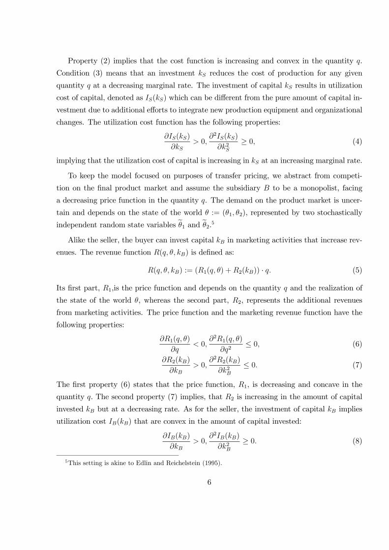
Property (2) implies that the cost function is increasing and convex in the quantity q.
Condition (3) means that an investment kS reduces the cost of production for any given
quantity q at a decreasing marginal rate. The investment of capital kS results in utilization
cost of capital, denoted as IS(kS) which can be different from the pure amount of capital in-
vestment due to additional efforts to integrate new production equipment and organizational
changes. The utilization cost function has the following properties:
∂IS(kS)
∂kS> 0,
∂2IS(kS)
∂k2S≥ 0, (4)
implying that the utilization cost of capital is increasing in kS at an increasing marginal rate.
To keep the model focused on purposes of transfer pricing, we abstract from competi-
tion on the final product market and assume the subsidiary B to be a monopolist, facing
a decreasing price function in the quantity q. The demand on the product market is uncer-
tain and depends on the state of the world θ := (θ1, θ2), represented by two stochastically
independent random state variables θ̃1 and θ̃2.5
Alike the seller, the buyer can invest capital kB in marketing activities that increase rev-
enues. The revenue function R(q, θ, kB) is defined as:
R(q, θ, kB) := (R1(q, θ) +R2(kB)) · q. (5)
Its first part, R1,is the price function and depends on the quantity q and the realization of
the state of the world θ, whereas the second part, R2, represents the additional revenues
from marketing activities. The price function and the marketing revenue function have the
following properties:
∂R1(q, θ)
∂q< 0,
∂2R1(q, θ)
∂q2≤ 0, (6)
∂R2(kB)
∂kB> 0,
∂2R2(kB)
∂k2B≤ 0. (7)
The first property (6) states that the price function, R1, is decreasing and concave in the
quantity q. The second property (7) implies, that R2 is increasing in the amount of capital
invested kB but at a decreasing rate. As for the seller, the investment of capital kB implies
utilization cost IB(kB) that are convex in the amount of capital invested:
∂IB(kB)
∂kB> 0,
∂2IB(kB)
∂k2B≥ 0. (8)
5This setting is akine to Edlin and Reichelstein (1995).
6

The financial subsidiary’s scope of business is to provide capital to subsidiaries B and S
to fund their investments. Subsidiary F serves solely as an internal capital provider without
any decision-making authority. In exchange for capital kB and kS, subsidiaries B and S
have to pay the financing company an interest rate of r ∈ [r;_r] per unit of capital, referred
to as capital transfer price (CTP). The lower bound r represents the interest rate at which
subsidiary F can raise funds from the global capital market, the upper bound_r is the
maximum rate accepted by the tax authorities. Further we assume the lower bound of the
capital transfer price to be constant and independent of kB and kS.6 Likewise, we define an
acceptable range for the product transfer price t ∈ [t, t], such that t lies between marginal
production cost t = ∂C(q, kS)/∂q and the market price per unit of the final product t = p.
Due to the MNC’s possibility to raise funds from the global capital market, it faces few
restrictions for its financing subsidiary’s location. In order to benefit from tax savings, the
company has a vested reason to place subsidiary F in a country where the tax rate on
interest income is as low as possible. In contrast, the MNC might face more legal, political
and organizational restrictions for the location of its HQ. This finally makes a legally separate
and delocated financing subsidiary plausible and allows us to set the financing company’s
tax rate τF equal to zero. We define the effective tax rate for subsidiary S as τ ≥ 0 and the
one for subsidiary B as τ + δ ≥ 0, with δ ∈ [−τ ; 1− τ ].
The timeline of events and the information structure about the realization of the state
of the world θ is as follows:
[Please insert figure 1 about here]
The timeline starts with the HQ’s decision on the capital and the product transfer price,
r and t. At date t = 2, subsidiaries B and S observe the realization of the state variable θ̃1,
that gives them better, though not precise information about the product demand. Based on
that private information, they decide in t = 3 on the optimal amounts of capital investments
kB and kS. At date t = 4, subsidiary B observes the realization of θ̃2. Thus, subsidiary
B has full information about the product demand and decides at date t = 5 about the
optimal quantity ordered from subsidiary S. At the last stage, the transfer of q units of the
6We abstract from the case where the amount of capital raised influences the interest rate and assume the
group’s overall financing conditions on the global capital market to be independent of the concrete amount
of capital raised.
7
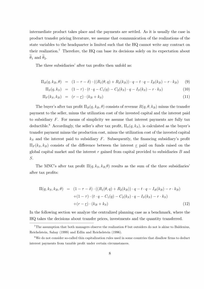
intermediate product takes place and the payments are settled. As it is usually the case in
product transfer pricing literature, we assume that communication of the realizations of the
state variables to the headquarter is limited such that the HQ cannot write any contract on
their realization.7 Therefore, the HQ can base its decisions solely on its expectation about
θ̃1 and θ̃2.
The three subsidiaries’after tax profits then unfold as:
ΠB(q, kB, θ) = (1− τ − δ) · ((R1(θ, q) +R2(kB)) · q − t · q − IB(kB)− r · kB) (9)
ΠS(q, kS) = (1− τ) · (t · q − C1(q)− C2(kS) · q − IS(kS)− r · kS) (10)
ΠF (kS, kB) = (r − r) · (kB + kS) (11)
The buyer’s after tax profit ΠB(q, kB, θ) consists of revenue R(q, θ, kB) minus the transfer
payment to the seller, minus the utilization cost of the invested capital and the interest paid
to subsidiary F . For means of simplicity we assume that interest payments are fully tax
deductible.8 Accordingly, the seller’s after tax profit, ΠS(q, kS), is calculated as the buyer’s
transfer payment minus the production cost, minus the utilization cost of the invested capital
kS and the interest paid to subsidiary F . Subsequently, the financing subsidiary’s profit
ΠF (kS, kB) consists of the difference between the interest r paid on funds raised on the
global capital market and the interest r gained from capital provided to subsidiaries B and
S.
The MNC’s after tax profit Π(q, kS, kB,θ) results as the sum of the three subsidiaries’
after tax profits:
Π(q, kS, kB, θ) = (1− τ − δ) · ((R1(θ, q) +R2(kB)) · q − t · q − IB(kB)− r · kB)
+(1− τ) · (t · q − C1(q)− C2(kS) · q − IS(kS)− r · kS)
+(r − r) · (kB + kS) (12)
In the following section we analyze the centralized planning case as a benchmark, where the
HQ takes the decisions about transfer prices, investments and the quantity transferred.
7The assumption that both managers observe the realization θ but outsiders do not is akine to Baldenius,
Reichelstein, Sahay (1999) and Edlin and Reichelstein (1996).8We do not consider so-called thin capitalization rules used in some countries that disallow firms to deduct
interest payments from taxable profit under certain circumstances.
8

3 Centralized planning (benchmark case)
As benchmark, we analyze a setting of centralized planning where the headquarter takes
all decisions, i.e. the HQ determines the quantity q transferred between B and S, the
subsidiaries capital investments kB and kS, the product transfer price t and the capital
transfer price r. The HQ, unlike the managers of subsidiaries B and S, cannot observe the
realizations of the state variables θ̃1 and θ̃2 and has to base its decisions on expectations
E[θ̃1] and E[θ̃2]. Therefore the group’s expected profit results as:
Eθ[Π(q, kS, kB, θ)] = (1− τ − δ) · (Eθ[R1(θ, q) · q] +R2(kB) · q − IB(kB))
+(1− τ) · (−C1(q)− C2(kS) · q − IS(kS))
+δ · t · q + (r · τ − r) · kS + (r · (τ + δ)− r) · kB (13)
Because the HQ takes all decisions based on the same information the decision process
can be modeled as a simultaneous optimization problem. Maximizing the group’s expected
profit to the capital and product transfer price yields the following optimality conditions:
∂Eθ[Π(q, kS, kB, θ)]
∂r= τ · kS + (τ + δ) · kB ≥ 0 (14)
∂Eθ[Π(q, kS, kB, θ)]
∂t= δ · q. (15)
Inspecting the above conditions (14) and (15) we derive our first proposition:
Proposition 1: In the centralized case, the optimal CTP and the optimal PTP are set
independently of each other. The optimal CTP is set at the upper bound of the admissible
interval, r = r, and the optimal PTP is set at the upper (lower) bound t = t ( t = t) for
a positive (negative) tax rate difference δ > 0 ( δ < 0). If the tax rate difference between
subsidiaries B and S is zero, δ = 0, the optimal PTP has no effect on the expected profit
and can be set arbitrarily between t and t.
Proof: Results directly from the FOC’s (14) and (15).
Condition (14) is positive for all levels of capital investments kB and kS and represents the
group’s tax benefit from shifting profits to the financing subsidiary that has the lowest tax
rate within the group. The similar argument holds for the product transfer price. Condition
9
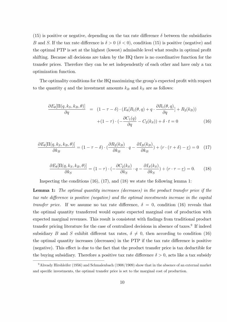
(15) is positive or negative, depending on the tax rate difference δ between the subsidiaries
B and S. If the tax rate difference is δ > 0 (δ < 0), condition (15) is positive (negative) and
the optimal PTP is set at the highest (lowest) admissible level what results in optimal profit
shifting. Because all decisions are taken by the HQ there is no coordinative function for the
transfer prices. Therefore they can be set independently of each other and have only a tax
optimization function.
The optimality conditions for the HQmaximizing the group’s expected profit with respect
to the quantity q and the investment amounts kB and kS are as follows:
∂Eθ[Π(q, kS, kB, θ)]
∂q= (1− τ − δ) · (Eθ[R1(θ, q) + q · ∂R1(θ, q)
∂q] +R2(kB))
+(1− τ) · (−∂C1(q)∂q
− C2(kS)) + δ · t = 0 (16)
∂Eθ[Π(q, kS, kB, θ)]
∂kB= (1− τ − δ) · (∂R2(kB)
∂kB· q − ∂IB(kB)
∂kB) + (r · (τ + δ)− r) = 0 (17)
∂Eθ[Π(q, kS, kB, θ)]
∂kS= (1− τ) · (−∂C2(kS)
∂kS· q − ∂IS(kS)
∂kS) + (r · τ − r) = 0. (18)
Inspecting the conditions (16), (17), and (18) we state the following lemma 1:
Lemma 1: The optimal quantity increases (decreases) in the product transfer price if the
tax rate difference is positive (negative) and the optimal investments increase in the capital
transfer price. If we assume no tax rate difference, δ = 0, condition (16) reveals that
the optimal quantity transferred would equate expected marginal cost of production with
expected marginal revenues. This result is consistent with findings from traditional product
transfer pricing literature for the case of centralized decisions in absence of taxes.9 If indeed
subsidiary B and S exhibit different tax rates, δ 6= 0, then according to condition (16)
the optimal quantity increases (decreases) in the PTP if the tax rate difference is positive
(negative). This effect is due to the fact that the product transfer price is tax deductible for
the buying subsidiary. Therefore a positive tax rate difference δ > 0, acts like a tax subsidy
9Already Hirshleifer (1956) and Schmalenbach (1908/1909) show that in the absence of an external market
and specific investments, the optimal transfer price is set to the marginal cost of production.
10

and makes the transfer of a higher quantity favorable. The same logic applies to a negative
tax rate difference δ < 0.
Inspecting the two conditions (17) and (18) reveal that in absence of tax rate differences
between the operating subsidiaries B and S and the financing subsidiary F , that is τ =
0 and δ = 0, the optimal investment levels would equate the expected marginal returns
with expected marginal investment costs. In the case of a tax rate difference, the optimal
investment amounts increase in the capital transfer price r. Like for the product transfer
price, the effect is due to a tax saving effect. The capital transfer price paid to the financing
subsidiary is tax deductible for the investing subsidiaries and thus makes higher investments
more favorable because of the lower taxes that have to be paid. Since we assumed a tax rate
of zero for the financing subsidiary, this effect is always positive.
The key element for these two effects of the product and capital transfer price is that
all decisions are taken centrally. This means that the two transfer prices only have a tax
shifting function but are not vital to coordinate optimal decisions. In conclusion, since both
transfer prices are solely used for profit shifting and the investments and the quantity are
set by the HQ, the two transfer prices can be set independent of each other.
The effect of a CTP on the optimal quantity q, the optimal investment levels kB and kSand the product transfer price t for the case where δ > 0 is depicted in figure 2.
[Please insert figure 2 about here]
Figure 2 particularly highlights the aforementioned observation from lemma 1 that an
increase of the CTP r leads to higher optimal investments kB and kS due to profit shifting.
The increase in investments from a higher CTP is eventually limited by the upper bound
r, the maximum rate accepted by the tax authority. Higher investments in turn reduce
marginal cost of production and increase marginal revenues and thus lead to a higher quantity
transferred. Since the PTP t serves solely as a means to shift profits, t is set at the highest
level because of the assumed positive tax rate difference δ and is independent of the level of
the CTP r. Concisely, in the centralized setting, the two types of transfer prices only serve
to minimize tax payments and do not intervene with each other.
In the following section we analyze the effects on the optimal solutions in the case of
decentralized quantity and investment decisions.
11

4 Decentralized quantity and investment decisions
In the decentralized case, the HQ assigns the investment decisions to the subsidiaries B and
S and provides the buyer with the authority to set the quantity transferred. The motivation
to delegate these decisions is based on the assumption that the HQ cannot observe the
realization of the state variables θ̃1 and θ̃2. The subsidiaries indeed benefit from private
information and sequentially learn the realization of the state variables. In t = 2, both
subsidiaries observe the realization of the state variable θ̃1 before, in t = 3, they have to
decide about their respective capital investments. After the investment decision, subsidiary
B receives additional private information about the realization of the state variable θ̃2.
Observing θ1 and θ2, subsidiary B learns the true demand in the product market. Since
the subsidiaries of a MNC generally face multiple projects where in turn each project might
request a wide range of investment decisions it seems reasonable to assume that an elaborated
communication of all private information to the HQmight not be feasible or simply too costly.
In such a setting, the delegation of investment decisions from the headquarter to the better
informed subsidiaries may finally increase investment and process effi ciency.10
In order to solve the optimization problem for the sequential decision structure, we apply
backward induction. At the last stage subsidiary B maximizes its profit ΠB w.r.t. the
quantity q, yielding the optimality condition:
∂ΠB(q, kB, θ)
∂q= R1(q, θ) + q · ∂R1(q, θ)
∂q+R2(kB)− t = 0. (19)
Comparing condition (19) to the optimality condition in the centralized case (16) we observe
two differences from delegating the quantity decision to subsidiary B. First, condition (19)
is based on the realization of θ, respectively θ1 and θ2, instead of its expectation. Second,
the optimality condition (19) implies that the quantity decision now also depends on the
product transfer price t. We state these observations in the following lemma.
Lemma 2: In the case of decentralized quantity decision the optimal quantity q is decreasing
in the product transfer price t and increasing in the amount of invested capital kB.
We face the traditional coordination problem. The optimal quantity under decentralized
versus centralized planning is of equal amount if the product transfer price t is set to marginal
10The assumption of asymmetric information that arises from too costly or impossible communication of
all local information to the central management has already been mentioned in Kaplan & Atkinson (1998,
p. 291) as one major reason to decentralize decisions.
12

cost. If t exceeds marginal cost, the optimal quantity in the decentralized setting is lower
than in the centralized case. On the one hand, this effect stems from a higher t inducing
higher marginal costs for subsidiary B. On the other hand, unlike the HQ in the benchmark
case, subsidiary B does not internalize the group’s benefit from tax savings by shifting
profits to the lowest taxed subsidiary. Instead, subsidiary B bases its decision about the
quantity q only on its own profit and neglects the other subsidiaries’profits as well as the
overall benefit for the MNC. Consequently, subsidiary B’s decision on the optimal quantity
q◦(θ) := q(θ1, θ2, kB, t) depends solely on its marginal return, that in turn is a positive
function of the investment level kB, the product transfer price t as well as the realization of
the state variables θ̃1 and θ̃2.
Quite intuitively, in the prevailing model setting with asymmetric information and dele-
gated investment decisions, both subsidiaries set the investment amounts in order to optimize
their profits, given their information θ1 about the demand in the product market. In the
centralized case where the headquarter lacks this private information and bases its decisions
on expectations, the HQ is more likely to prescribe ineffi cient investment amounts. In that
respect, the delegation of the investment decisions to the subsidiaries may increase invest-
ment effi ciency but lead to divisional instead of overall profit maximization. The respective
optimality conditions of the subsidiaries w.r.t. the capital investments in the decentralized
case are as follows:
∂Eθ2[ΠB(q
◦(θ), kB, θ)
]∂kB
= Eθ2 [q◦(θ)] · ∂R2(kB)
∂kB− ∂IB(kB)
∂kB− r = 0, (20)
∂Eθ2[ΠS(q
◦(θ), kS)
]∂kS
= −Eθ2 [q◦(θ)] · ∂C2(kS)
∂kS− ∂IS(kS)
∂kS− r = 0. (21)
The optimal investment amounts k◦B := kB(Eθ2 [q
◦(θ)], r) and k
◦S := kS(Eθ2 [q
◦(θ)], r)
depend on the expected quantity and the capital transfer price. Both subsidiaries know
θ1 but at the time the investment decisions have to be reached the realization of θ̃2 is
still unknown. Therefore, subsidiaries B and S have to base their investment decisions on
expectations about the true demand. Considering the optimality conditions (20) and (21),
the capital transfer price r represents additional marginal investment costs to divisions B
and S. Thus a higher capital transfer price makes capital investments more costly and will in
turn reduce the subsidiaries investment incentives. We summarize this effect in the following
lemma 3.
13

Lemma 3: The optimal capital investments kB(Eθ2 [q◦(θ)], r) and kS(Eθ2 [q
◦(θ)], r) are de-
creasing in the capital transfer price r.
This is in contrast to the optimality conditions (17) and (18) in the centralized decision
case. In the benchmark the HQ prescribes the investment amounts and the group benefits
from a higher CTP due to profit shifting, respectively tax savings. In the decentralized
setting, the subsidiaries first care about their divisional profits and indeed neglect the group’s
tax benefits and the effects on the other subsidiaries’ profits when deciding about their
respective capital investments. Consequently, in the decentralized planning case, the effect
of r on the optimal investments is negative and is in the opposite direction compared to the
centralized setting.
In the final step of the optimization process, the HQ sets the capital transfer price r as well
as the product transfer price t to maximize the group’s expected profit Eθ[Π(q◦(θ), k
◦B, k
◦S, θ)].
To shorten notation we define Vθ(q◦, k
◦B, k
◦S) := Eθ[Π(q
◦(θ), k
◦B, k
◦S, θ)]. Maximizing the
group’s expected profit w.r.t. the capital and product transfer price, yields the following
optimality conditions:
∂Vθ(q◦, k
◦B, k
◦S)
∂r= Eθ[(τ + δ) · k◦B + τ · k◦S
+(1− τ) · (t− (∂C1(q
◦(θ))
∂q− C2(k
◦
S))) · ∂q∂kB
· ∂kB∂r
+(r − r) · ∂(k◦B + k
◦S)
∂r] = 0, (22)
∂Vθ(q◦, k
◦B, k
◦S)
∂t= Eθ[δ · q
◦(θ) + (1− τ) · (t− (
∂C1(q◦(θ))
∂q− C2(k
◦
S))) · ( ∂q∂kB
· ∂kB∂t
+∂q
∂t)
+(r − r) · ∂(k◦B + k
◦S)
∂t] = 0. (23)
Solving these FOC’s for r and t results in an optimal CTP r◦
:=r(Eθ[q◦(θ), k
◦B, k
◦S, θ])
and an optimal PTP t◦
:= t(Eθ[q◦(θ), k
◦B, k
◦S, θ]) being functions of the expectations about
the optimal quantity, the optimal investment amounts and the realization of the state of
the world. Inspecting the optimality conditions (22) and (23) we observe that the optimal
transfer prices are influenced by three distinct effects.
14

The optimal capital and product transfer prices r◦and t
◦balance a tax effect with two
negative coordination effects on the optimal quantity and the optimal capital investments.
The first term in the optimality conditions (22) and (23) represents the tax effect. This effect
is due to the transfer prices’serving as means to shift profits. With respect to the capital
transfer price, the profit is always shifted to the financing subsidiary and the tax effect is
unambiguously positive. For the product transfer price, the tax effect depends on the tax
rate difference δ between the subsidiaries B and S and can either be positive or negative.
The second term we refer to as quantity coordination effect. For the capital transfer price,
this effect is negative. Lemma 3 states that a higher capital transfer price reduces the
capital investment, ∂kB/∂r < 0, since the capital transfer price r represents additional
costs to the subsidiaries. Lemma 2 states that a higher capital investment increases the
quantity, ∂q/∂kB > 0. Therefore, the second term in condition (22) is strictly negative.
For the product transfer price, this effect is also negative as Lemma 2 states that a higher
product transfer price decreases the quantity, ∂q/∂t < 0. Finally, we observe a third effect
that we refer to as investment coordination effect. As aforementioned, with respect to the
capital transfer price, Lemma 3 states that a higher capital transfer price reduces investment
incentives. However, for the product transfer price we face an indirect effect on the optimal
capital investments that arises from the decision about the optimal quantity. Condition (19)
shows that a higher product transfer price decreases the optimal quantity and thus decreases
marginal investment returns what finally decreases optimal investments.
Comparing the optimality conditions in the decentralized setting (22) and (23) to the
conditions in the centralized case (14) and (15), the first term that is related to the direct tax
effect is similar. The two additional effects, the quantity and investment coordination effects,
result from delegating the quantity and investment decisions to the subsidiaries. While the
coordination of quantity and investment decisions is not necessary in the centralized setting,
a trade-off results in the decentralized case. The headquarter has to balance the positive tax
effect from higher transfer prices with the negative effects on the investment decisions and the
quantity decision. Because the subsidiaries B and S maximize their respective profits and
not the group’s profit, they face an increase in their marginal costs (intermediate product
and capital) but they do not internalize the tax benefits for the whole MNC from profit
shifting. Compared to the centralized setting, the two additional effects are thus weakly
negative and the resulting optimal product and capital transfer prices in the decentralized
setting are weakly lower than in the centralized case.
15

In addition, the optimality conditions (22) and (23) show that the CTP and PTP are no
longer independent of each other. We summarize this interrelation between the two transfer
prices in proposition 2.
Proposition 2: The optimal CTP and PTP negatively relate to each other, i.e. the optimal
CTP is decreasing in the optimal PTP and vice versa.
Proof: The second term of condition (22), we referred to as quantity coordination effect, is
negative in r and is scaled by the difference between t and the marginal cost. Therefore, a
higher product transfer price t intensifies the negative quantity coordination effect of r. The
proof for the PTP is similar. The third term in condition (23) represents the investment
coordination effect of the optimal product transfer price. This effect is negative in t and
is scaled by the difference between the capital transfer price and the interest paid on the
capital market. A higher capital transfer price r thus intensifies the negative investment
coordination effect of t.
The intuition for the interaction between the two transfer prices is straight forward. The
optimal capital transfer price internalizes the negative effect on the optimal investment kBthat results in a lower quantity. This effect is scaled by the difference between the product
transfer price and the marginal cost. If the product transfer price is equal to the marginal
cost, the quantity coordination effect is zero. A higher product transfer price results in a
higher quantity coordination effect that intensifies the negative effect on the capital transfer
price.
The intuition for the product transfer price is akin. The optimal product transfer price
internalizes the effect on the quantity and the resulting indirect effect on the capital invest-
ments kB and kS. This effect is scaled by the difference between the capital transfer price and
marginal cost of capital. If the capital transfer price is equal to the marginal cost of capital,
the investment effect is zero. A higher capital transfer price results in a higher investment
coordination effect that intensifies the negative effect on the product transfer price.
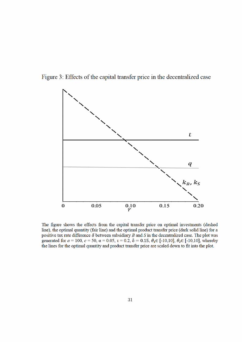
Figure 3 illustrates these effects of r on the optimal investment amounts, the optimal
quantity transferred and the PTP, again for the case δ > 0.
[Please insert figure 3 about here]
To sum up, in the case of decentralized quantity and investment decisions, implementing
a capital transfer price benefits the group from saving taxes via profit shifting, but leads
16

to lower investments, distorted managerial decisions, a negative effect on the PTP and its
respective tax savings.
5 A parametric example
In this section we provide a parametric example to illustrate the relations between the two
transfer prices, the impact of different tax rates and consequences of the decision to centralize
or decentralize.
For means of simplicity we assume the random state variable θ̃ to be a sum of θ̃1 and θ̃2,
where θ̃1 and θ̃2 are uncorrelated, uniformly distributed over an interval [−ξ, ξ] and exhibitan expected value of E[θ̃l] = 0 and a variance of V ar(θ̃l) = 1/12 · (ξ − (−ξ))2, for l ∈ {1, 2}.Further we assume quadratic utilization cost of capital Ii(ki) = γ · k2i , i ∈ {B, S}, where γis a scaling parameter. The revenue function for the buyer is specified as:
R(q, θ1, θ2, kB) = (R1(θ1, θ2, q) +R2(kB)) · q
= (a+ θ1 + θ2 − q + α · kB) · q (24)
and the seller’s cost of production is given by:
C(q, kS) = C1(q) + C2(kS) · q
= (c− α · kS) · q, (25)
where the scaling parameter α represents the investment effi ciency. The profit functions
of buyer B and seller S then unfold as:
ΠB(q, kB, θ1, θ2, t, r) = (1− τ − δ) · (R(q, θ1, θ2, kB)− t · q − IB(kB)− r · kB)
= (1− τ − δ) · ((a+ θ − q + α · kB − t) · q − γ · k2B − r · kB),(26)
ΠS(q, kS, t, r) = (1− τ) · (t · q − C(q, kS)− IS(kS)− r · kS)
= (1− τ) · ((t− c+ α · ks) · q − γ · k2S − r · kS). (27)
The profit function of the financial subsidiary F remains as in the general model and the
MNC’s profit function is simply the sum of the three subsidiaries profit functions.
17

5.1 The centralized case
In the centralized setting, the HQ sets the following optimal quantity q∗ according to condi-
tion (16) as:
q∗ =1
2· (a+ α · k∗B +
δ · t∗ + (1− τ) · (α · k∗S − c)(1− τ − δ) ). (28)
The parametric representation of the optimal quantity q∗supports lemma 1. The optimal
quantity increases (decreases) in the product transfer price if the tax rate difference δ is
positive (negative). Because the HQ takes its decisions based on the expectation about the
state variable θ̃, the quantity decision is not affected by the realization of θ. Further, from
equation (??) we observe that the decision about the optimal quantity depends also on the
capital investments. Plugging the parametric functions into the optimality conditions (17)
and (18), yields the following conditions on the optimal capital investments:11
∂Eθ[Π(q∗, kB, kS, θ)]
∂kB= (1− τ − δ) · (α · q∗ − 2 · γ · k∗B) + (τ + δ) · r∗ − r = 0, (29)
∂Eθ[Π(q∗, kB, kS, θ)]
∂kS= (1− τ) · (α · q∗ − 2 · γ · k∗S) + τ · r∗ − r = 0. (30)
Inspecting the above conditions (29) and (30), we find that the optimal capital invest-
ments increase in the capital transfer price r∗ what supports lemma 1. As mentioned above,
this effect results from a higher capital transfer price shifting taxes to the lowest taxed
subsidiary F . This finally makes higher investments more attractive for the MNC.
In this setting, the HQ also takes the decisions about the optimal transfer prices. The
resulting optimality conditions are identical to the benchmark case (see (14) and (15)).
These two conditions, (14) and (15), accede proposition 1. The two transfer prices can
be set independently of each other. The optimal capital transfer price is set at the upper
bound of the admissible interval r and the optimal product transfer at the upper or lower
level of the admissible interval, depending on the tax rate difference δ.
11One could solve these equations for the optimal investment amounts being aware that q∗ is in turn a
function of kB and kS . We forego this step due to the more intuitive representation of the interdependences
out of the FOC.
18

5.2 The decentralized case
In the decentralized setting the optimal quantity is denoted by q◦. The subsidiary B chooses
the optimal quantity according to the optimality condition (19). Using the parameterization
we derive the following optimal quantity:
q◦(θ) =
1
2· (a+ α · k◦B − t
◦+ θ1 + θ1). (31)
Comparing the optimal quantity q◦to the one in the centralized case (28), we find that
the optimal quantity q◦does not depend on the tax rates. Because subsidiary B does not
internalize the group’s tax benefits of profit shifting, the tax rate differences are not relevant
for the subsidiary‘s quantity decision. Further, as stated in lemma 2, the optimal quantity
q◦ decreases in the product transfer price t◦since a higher PTP represents higher costs to
the buyer. As a consequence of subsidiary B’s private information about the final demand,
the realization of the state variable θ directly affects the buyer’s decision about the optimal
quantity q◦(θ). Finally, the optimal quantity increases in subsidiary B’s capital investment
kB because it increases the product’s marginal revenues.
Applying the parametric specifications to the optimality conditions (20) and (21) yields:
∂Eθ2[ΠB(q
◦(θ), kB, θ)
]∂kB
= α · Eθ2 [q◦(θ)]− 2 · γ · k◦B − r
◦= 0, (32)
∂Eθ2[ΠS(q
◦(θ), kS)
]∂kS
= −α · Eθ2 [q◦(θ)]− 2 · γ · k◦S − r
◦= 0. (33)
Solving the optimality conditions yields the following optimal investment amounts:
k◦
B = k◦
S =α · (a− t◦ + θ1)− 2 · r◦
4 · γ − α2 . (34)
While in the centralized setting the optimal investments depend on the tax rates, they
do not rely on tax issues in the decentralized case. In that respect, the parametric example
shows that the subsidiaries do not internalize the opportunity to shift profits. In the decen-
tralized case, the capital transfer price represents additional cost to subsidiaries B and S
and leads to a decrease in the optimal investment amounts. Because the subsidiaries observe
the realization of θ̃1 their decision about the respective investments is directly affected by
19
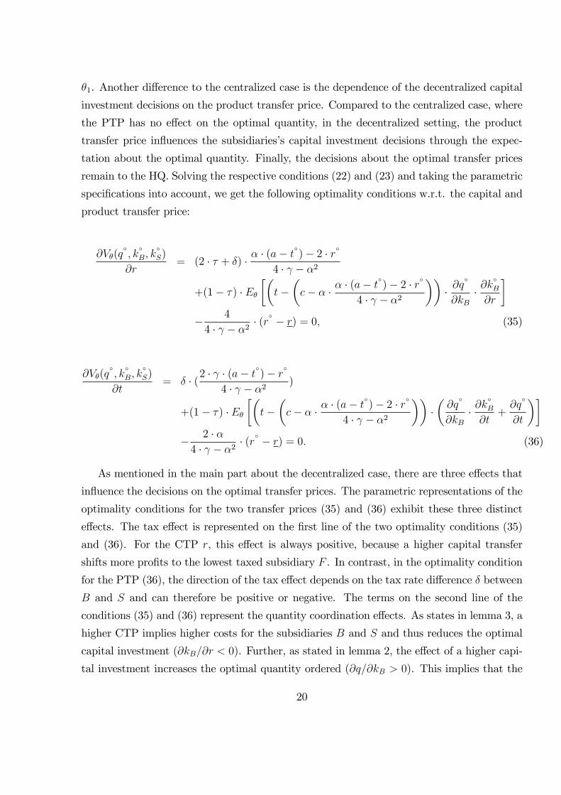
θ1. Another difference to the centralized case is the dependence of the decentralized capital
investment decisions on the product transfer price. Compared to the centralized case, where
the PTP has no effect on the optimal quantity, in the decentralized setting, the product
transfer price influences the subsidiaries’s capital investment decisions through the expec-
tation about the optimal quantity. Finally, the decisions about the optimal transfer prices
remain to the HQ. Solving the respective conditions (22) and (23) and taking the parametric
specifications into account, we get the following optimality conditions w.r.t. the capital and
product transfer price:
∂Vθ(q◦, k
◦B, k
◦S)
∂r= (2 · τ + δ) · α · (a− t
◦)− 2 · r◦
4 · γ − α2
+(1− τ) · Eθ[(t−(c− α · α · (a− t
◦)− 2 · r◦
4 · γ − α2
))· ∂q
◦
∂kB· ∂k
◦B
∂r
]− 4
4 · γ − α2 · (r◦ − r) = 0, (35)
∂Vθ(q◦, k
◦B, k
◦S)
∂t= δ · (2 · γ · (a− t◦)− r◦
4 · γ − α2 )
+(1− τ) · Eθ[(t−(c− α · α · (a− t
◦)− 2 · r◦
4 · γ − α2
))·(∂q
◦
∂kB· ∂k
◦B
∂t+∂q
◦
∂t
)]− 2 · α
4 · γ − α2 · (r◦ − r) = 0. (36)
As mentioned in the main part about the decentralized case, there are three effects that
influence the decisions on the optimal transfer prices. The parametric representations of the
optimality conditions for the two transfer prices (35) and (36) exhibit these three distinct
effects. The tax effect is represented on the first line of the two optimality conditions (35)
and (36). For the CTP r, this effect is always positive, because a higher capital transfer
shifts more profits to the lowest taxed subsidiary F . In contrast, in the optimality condition
for the PTP (36), the direction of the tax effect depends on the tax rate difference δ between
B and S and can therefore be positive or negative. The terms on the second line of the
conditions (35) and (36) represent the quantity coordination effects. As states in lemma 3, a
higher CTP implies higher costs for the subsidiaries B and S and thus reduces the optimal
capital investment (∂kB/∂r < 0). Further, as stated in lemma 2, the effect of a higher capi-
tal investment increases the optimal quantity ordered (∂q/∂kB > 0). This implies that the
20
quantity coordination effect for the optimal CTP is unambiguously negative - as long as the
PTP exceeds marginal cost of production. If the PTP is identical to marginal production
cost, the effect becomes zero as in the standard transfer pricing model. Considering lemma
2 and lemma 3 and the fact, that ∂q/∂t < 0, the argumentation for the product transfer
price is similar. Finally, the third line in the conditions (35) and (36) represent the invest-
ment coordination effect. This effect is always negative because the investment amount is
decreasing in both transfer prices.
5.3 Some comparative statics
In order to analyze the effects of a variation in the tax rate difference and the uncertainty
about the state of the world, we conduct a numerical example with the following specifica-
tions:
τ = 0.2, δ ∈ [−0.15, 0.15], θ1 ∈ [−10, 10], θ2 ∈ [−10, 10], t = 70, r = 0.25, r = 0,
a = 100, c = 50, α = 0.05, γ = 0.05.
Solving the optimality conditions for the decision variables derived in the sections 5.2
and 5.3 for the centralized and decentralized case, we get the following results:
[Please insert table 1 about here]
First, we analyze the results for the centralized case. According to proposition 1 the two
transfer prices just have a tax saving function and are set at the bounds of the admissible
intervals. Because the financing subsidiary has a tax rate of zero, the capital transfer price
is set at the upper bound. The optimal product transfer price depends on the tax rate
difference δ between the subsidiaries and is set at the lower bound that is equal to marginal
cost for δ < 0 and at the upper bound for δ > 0. Both transfer prices are independent of
each other and only react to tax rate differences.
The optimal quantity increases in the product transfer price when the tax rate difference
becomes positive. This effect is stated in lemma 1 and is due to tax shifting opportunities
once the PTP is above marginal cost. Because the CTP does not vary in the centralized
case with δ, the increase in the investments comes from the higher quantity that increases
21

marginal returns of the investments. Finally, the expected profit is decreasing in the tax rate
difference because the tax rate for subsidiary B is increasing what reduces after-tax profits.
Second, we analyze the results for the decentralized case. For a higher (less negative)
tax rate difference δ, higher investments become more favorable for the MNC because of tax
shifting opportunities. Higher investments are thus stimulated by a lower CTP. Because the
PTP is already set at marginal cost it can be decreased only marginally to the lower marginal
cost that are induced by higher investments. Increasing the tax rate difference further to
positive levels has two effects. First, the PTP increases due to the tax saving effect of profit
shifting between subsidiariesB and S. Second, the CTP further decreases as the coordination
effects become more negative in the higher PTP. These negatively interacting effects between
the transfer prices is described in proposition 2. The effects on the optimal quantity and the
optimal investments are stated in lemmas 2 and 3. The optimal quantity is decreasing in the
PTP as it represents additional cost to the buyer. This in turn decreases marginal returns
of the investments and leads to reduced optimal investment levels. Finally, the expected
profit is decreasing in higher tax rates like in the centralized case. What is different is
that the profit for a negative or zero tax rate difference is higher in the decentralized case
than with centralized decisions. This effect appears because of the information asymmetry
between the HQ and the subsidiaries. The HQ can base the quantity and the investment
decision only on expected information whereas the subsidiaries have partial information at
the date of the investment decision and full information at the date of the quantity decision.
Therefore, the numerical example shows that despite of negative coordination effects in
the decentralized setting, the decentralization of decisions can be beneficial in the case of
asymmetric information between the HQ and the subsidiaries.
We summarize the effects of the tax rate differences δ < 0, δ = 0 and δ > 0 on the
optimal transfer prices in the following table 2:
[Please insert table 2 about here]
A graphical representation of the dependence of the HQ’s decisions about the transfer
prices on the tax rate difference δ and ultimately of the interaction between those three
effects is depicted in figure 4.
[Please insert figure 4 about here]
22

The figure on the left hand side shows the positive interdependence between the tax rate
difference δ and the product transfer price. The higher the tax rate difference between the
subsidiaries B and S, the higher the profit shifting opportunity and thus the higher the PTP.
The PTP is however increasing in δ at a decreasing marginal rate due to the amplifying
negative quantity and investment coordination effects. In case of a tax rate difference of
δ ≤ 0, the PTP is set to marginal cost of production because the tax effect and the quantity
and investment coordination effect are all three negative. Since the PTP and CTP interact
negatively, the effect for the capital transfer price is in the opposite direction. While the
tax effect of the CTP is positive for all tax rate differences, the investment coordination
effect is negative for all δ and the quantity coordination effect on r is zero for δ ≤ 0 and
negative for positive tax rate differences. However, the positive tax effect decreases in δ
due to a higher tax rate difference increasing the PTP that in turn reduces the buyer’s
capital investment and the quantity ordered. Hence, the increasing negative investment
and quantity coordination effects push the CTP further down. If we assume an upper
border r for the acceptable range of the CTP we would get a cap at the accepted upper
range of r, preventing the capital transfer price to be set above that threshold when the
tax rate difference becomes low. The values for the capital and product transfer prices in
table 1 also support proposition 2 and show the negative mutual interdependence between
the two transfer prices. Recall, for a tax rate difference δ > 0, the group benefits from
a higher product transfer price due to the opportunity to shift profits from subsidiary B
to subsidiary S. As mentioned in lemma 2, this however reduces the quantity ordered
by subsidiary B (increases the negative quantity coordination effect) because a higher PTP
means higher cost to the buyer that in turn decreases the quantity ordered. A lower quantity
ordered in fact decreases also the marginal investment returns of subsidiary B (increases the
negative investment coordination effect) and we face decreasing optimal investments out
of the amplification through the two negative effects. As a consequence of lower capital
investments, the positive tax effect decreases and the quantity coordination effect gets even
more negative that in turn leads to a lower CTP. For a tax rate difference of δ ≤ 0, the
optimal PTP is always set to marginal cost of production since subsidiary B faces a lower
tax rate than subsidiary S, inducing the MNC to keep the buyer’s profits within division
B. Further, as mentioned above, increasing the capital transfer price means, for all tax
rate differences, higher investment cost to the subsidiaries B and S and thus lower optimal
capital investments (higher negative investment coordination effect). That in turn reduces
23

the optimal quantity because lower investments reduce buyer B’s marginal returns from
investments and this ultimately reduces the group’s tax savings (decrease in the positive
tax effect). Overall, the group’s benefit out of profit shifting decreases such that a higher
CTP finally leads to a lower product transfer price. We depict that interaction between the
capital and the product transfer prices for the decentralized case in the following figure.
[Please insert figure 5 about here]
Figure 5 pinpoints the negative relation between the two transfer prices, i.e. that the
increase of one transfer price decreases the other transfer price. An intersection sets in,
where the aforementioned effects of a higher CTP offset the effects resulting from a lower
PTP and vice versa.
Finally the question arises if the decentralized case can be beneficial to the MNC. The
results of our numerical example, presented in table 1, have already shown that decentral-
izing the quantity and the investment decision can be beneficial for the MNC. Because the
decentralization decision ultimately depends on the uncertainty about the true state of the
world θ, respectively the benefit of private information of the subsidiaries B and S, we finally
depict the expected decentralized profits for the group depending on the uncertainty about
the state variable θ̃, respectively θ̃1 and θ̃2, and compare it to the expected centralized profit.
Figure 6 illustrates the change in expected group profits due to changes in the variance of
the state variables for the tax rate differences δ = −0.15, δ = 0 and δ = 0.15.
[Please insert figure 6 about here]
In Figure 6, the solid lines represent the expected decentralized profits, whereby in each
of the three figures the lower solid lines represent the case where there is no uncertainty
about the state variable θ̃2 and the upper solid lines represent the case for a variance of
θ̃2 of V ar(θ̃2) = 100/312. The dashed lines represent the expected centralized profits that
are independent of the uncertainty about the state variable θ. As we would expect, the
benefit of decentralization increases in the uncertainty about the state of the world θ. This
is graphically represented by the positive slope of the solid lines and is the effect of the
12The Variance of a uniformly distributed random variable θ̃2 betweeen [−10, 10], is: V ar(θ̃2) = 1/12 ·(10− (−10))2 = 100/3.
24

subsidiaries private information about the realization of the state variable θ̃1. in addition,
the upward shift of the solid lines is the additional benefit of the two subsidiaries B and
S private information about the realization of the second state variable θ̃2. This parallel
upward shift is a consequence of the scaling of the variance of θ̃2 by (1 − τ − δ) > 0, so an
increase in V ar(θ̃2) just amplifies the results for the expected decentralized profits to the
upside. As table 1 has indicated, the decision to decentralize also depends on the tax rate
difference δ. For a tax rate difference of δ ≤ 0, the quantity coordination effect is zero and the
investment coordination effect is negative. Lower capital investments in turn decrease the
tax effect, since less profits are shifted to the lowest taxed subsidiary, the capital provider
F . In result, for a tax rate difference of δ ≤ 0, the benefit of better private information
might dominate the positive tax effect that results from shifting profits to subsidiary F .
However, with an increasing tax rate difference, the positive tax effect and the negative
investment coordination effect both get stronger. Further, for a tax rate difference of δ > 0
the group faces also the negative quantity coordination effect that decreases the benefits from
decentralization even more. Thus, these three effects might finally dominate the benefits of
private information leaving the MNC better off by keeping all decisions within the HQ.
6 Conclusion
With the raise of multinational companies and their possibilities to raise capital on the global
market and to place subsidiaries in different locations, international coordination, financing
opportunities and tax issues have become important. The public finance literature addresses
this issues mainly in research about capital transfers and its tax implications while the
managerial transfer pricing literature mainly addresses transfer pricing on physical products
and managerial issues. We try to fill the gap in research about interrelations between product
and capital transfer prices.
In the benchmark setting, where the MNC’s headquarter takes all decisions, we show
that the optimal capital and product transfer price are set independently of each other.
This result is in concurrence with the transfer pricing literature on physical products that
states that in this case the transfer price serves solely to save taxes and has no coordinative
function. Further, we show that optimal investments in the centralized setting with taxes
are larger than without taxes. This is due to the fact that interest payments on the capital
25
invested are tax deductible. We also find that the quantity ordered increases (decreases) in
the product transfer price for a negative (positive) tax rate difference between the supplying
and producing subsidiary.
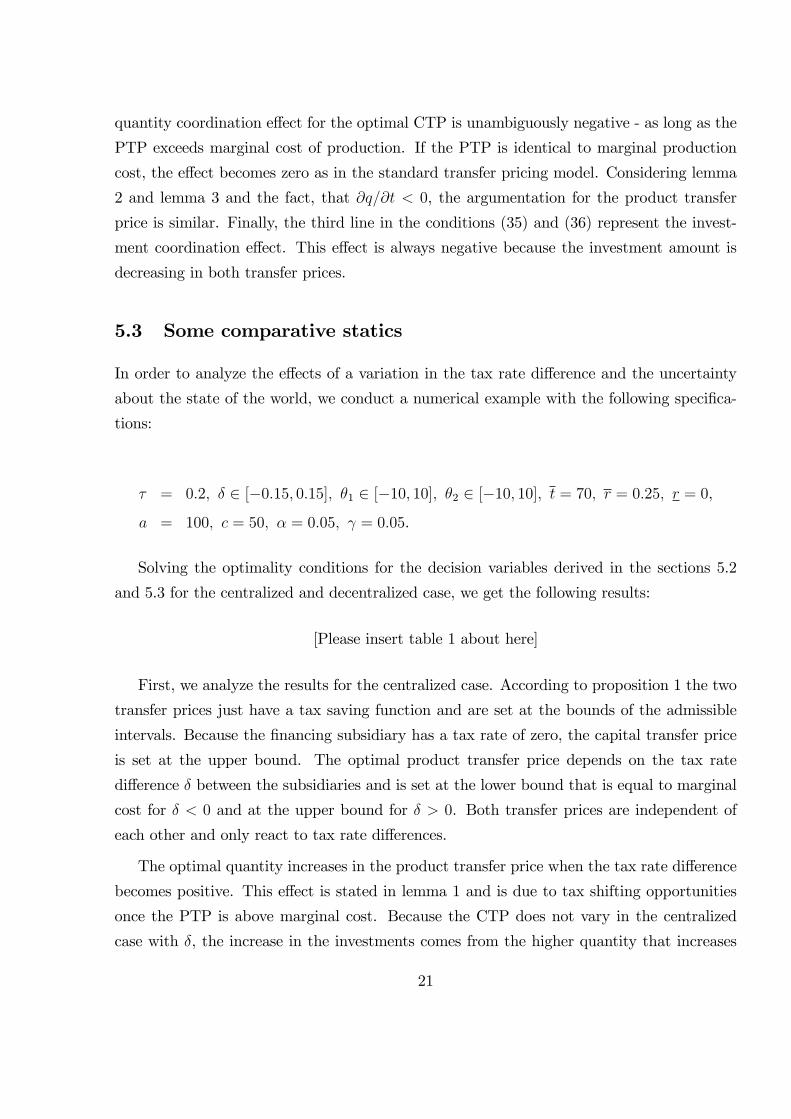
In the decentralized planning case, where quantity and investment decisions are delegated
to the operative subsidiaries of the multinational corporation, we find that transfer prices
do not just affect tax savings but entail additional coordinative effects on quantities and
investments. We show that those additional quantity and investment coordination effects
directly lead to lower quantities and investments, since the transfer prices represent marginal
costs to the buyer. Because the amount of capital invested ultimately affect marginal returns
and costs, we perceive an additional indirect effect on the quantity decision. In that respect,
we show that the two transfer prices are negatively related to each other. The intuition
for their negative interrelation is indeed found in the sequential decisions on investments
and quantities that have a negative impact on each other’s cost and returns. The key
findings is thus that the two transfer prices can no longer be set independent of each other
and the headquarter has to consider these interrelations while taking its decisions on the
optimal transfer prices. The amplitude of the three effects essentially depends on the tax
rate difference between the operative subsidiaries.
26

REFERENCES
Baldenius, T., Reichelstein, S., and Sahay, S. (1999). Negotiated versus cost-based transfer
pricing. Review of Accounting Studies, 4, 67—91.
Baldenius, T., Melumad, N., and Reichelstein, S. (2004). Integrating managerial and tax
objectives in transfer pricing. The Accounting Review, 79, 591-615.
Duerr, O.M. and Goex, R.F. (2011). Strategic incentives for keeping one set of books
in international transfer pricing. Journal of Economics & Management Strategy, 20,
269-298.
Duerr, O.M. and Goex, R.F. (2013). Specific investment and negotiated transfer pricing in
an international transfer pricing model. Schmalenbach Business Review, 65, 27-50.
Edlin, A.S. and Reichelstein, S. (1995). Specific investment under negotiated transfer
pricing: An effi ciency result. The Accounting Review, 70, 275-291.
Ernst & Young (2013): Navigating the choppy waters of international tax —2013 Global
Transfer Pricing Survey, http://www.ey.com/Publication/vwLUAssets/EY-2013_Global_
Transfer_Pricing_Survey/$FILE/EY-2013-GTP-Survey.pdf.
Goex, R.F. (2000): Strategic transfer pricing, Absorption Costing, and Observability. Man-
agement Accounting Research, 11, 327-348.
Goex, R.F. and Schiller, U. (2007). An economic perspective on transfer pricing. C.S.Chapman,
A.G. Hopwood, and M.D. Shields, ed., Handbook of Management Accounting Research
(Vol.2). Oxford: Elsevier, 673-693.
Grubert, H. (1998). Taxes and the division of foreign operating income among royalties,
interest, dividends and retained earnings. Journal of Public Economics, 68, 269-290.
Grubert, H. (2003). Intangible income, intercompany transactions income shifting, and the
choice of location. National Tax Journal, 56, 211-242.
Hirshleifer, J. (1956). On the economics of transfer pricing. Journal of Business, 29, 172-
184.
27

Johnson, N.B. (2006). Divisional performance measurement and transfer pricing for intan-
gible assets. Review of Accounting Studies, 11, 339-365.
Kaplan, R., and Atkinson, A.A. (1998). Advanced management accounting (3rd ed.).
Englewood Cliffs: Prentice-Hall.
Schmalenbach, E. (1908/1909). Über Verrechnungspreise. Zeitschrift für handelswirtschaftliche
Forschung, 3, 165—185.
Wagenhofer, A. (1994). Transfer pricing under asymmetric information —An evaluation of
alternative methods. European Accounting Review, 1, 71-104.
28

29

30
31

32

33

34
Related Documents