Constitutive modeling of static and cyclic behavior of interfaces and implementation in boundary value problems. Item Type text; Dissertation-Reproduction (electronic) Authors Navayogarajah, Nadarajah. Publisher The University of Arizona. Rights Copyright © is held by the author. Digital access to this material is made possible by the University Libraries, University of Arizona. Further transmission, reproduction or presentation (such as public display or performance) of protected items is prohibited except with permission of the author. Download date 13/07/2018 02:05:00 Link to Item http://hdl.handle.net/10150/185116

Welcome message from author
This document is posted to help you gain knowledge. Please leave a comment to let me know what you think about it! Share it to your friends and learn new things together.
Transcript

Constitutive modeling of static and cyclic behavior ofinterfaces and implementation in boundary value problems.
Item Type text; Dissertation-Reproduction (electronic)
Authors Navayogarajah, Nadarajah.
Publisher The University of Arizona.
Rights Copyright © is held by the author. Digital access to this materialis made possible by the University Libraries, University of Arizona.Further transmission, reproduction or presentation (such aspublic display or performance) of protected items is prohibitedexcept with permission of the author.
Download date 13/07/2018 02:05:00
Link to Item http://hdl.handle.net/10150/185116

INFORMATION TO USERS
The most advanced technology has been used to photograph and
reproduce this manuscript from the microfilm master. UMI films the
text directly from the original or copy submitted. Thus, some thesis and dissertation copies are in typewriter face, while others may be from any type of computer printer.
The quality of this reproduction is dependent upon the quality of the
copy submitted. Broken or indistinct print, colored or poor quality illustrations and photographs, print bleedthrough, substandard margins, and improper alignment can adversely affect reproduction.
In the unlikely event that the author did not send UMI a complete
manuscript and there are missing pages, these will be noted. Also, if unauthorized copyright material had to be removed, a note will indicate
the deletion.
Oversize materials (e.g., maps, drawings, charts) are reproduced by
sectioning the original, beginning at the upper left-hand corner and
continuing from left to right in equal sections with small overlaps. Each
original is also photographed in one exposure and is included in reduced form at the back of the book.
Photographs included in the original manuscript have been reproduced xerographically in this copy. Higher quality 6" x 9" black and white photographic prints are available for any photographs or illustrations
appearing in this copy for an additional charge. Contact UMI directly to order.
U-M-I University Microfilms International
A Beli & Howell Information Company 300 North Zeeb Road, Ann Arbor, M148106-1346 USA
313/761-4700 800/521-0600

t.

Order Number 9100045
Constitutive modeling of static and cyclic behavior of interfaces and implementation in boundary value problems
Navayogarajah, Nadarajah, Ph.D.
The University of Arizona, 1990
U·M·I 300 N. Zeeb Rd Ann Arbor, MI 48106

CONSTITUTIVE MODELING OF STATIC AND CYCLIC
BEHAVIOR OF INTERFACES AND
IMPLEMENTATION IN BOUNDARY VALUE PROBLEMS
by
N adarajah N avayogarajah
A Dissertation Submitted to the Faculty of the
DEPARTMENT OF CIVIL ENGINEERING AND ENGINEERING MECHANICS
In Partial Fulfillment of the Requirements For the Degree of
DOCTOR OF PHILOSOPHY WITH A MAJOR IN CIVIL ENGINEERING
In the Graduate College
THE UNIVERSITY OF ARIZONA
1990

THE UNIVERSITY OF ARIZONA GRADUATE COLLEGE
2
As members of the Final Examination Committee, we certify that we have read
the dissertation prepared by ____ ~N~a~d_a_ra~J~·a_h __ N_a_v~a~y_o~g~a_r_a~j_a_h ________________ ___
entitled Const i tut i ve Mode I ing of Stat ic and Cycl ic Behavior of
Interfaces and Implementation in Boundary Value Problems
and recommend that it be accepted as fulfilling the dissertation requirement
Doctor of Philosophy for the Degree of -------------------------------------------------------
C. s. Desa i Date
?~/2 / ' panosD.~~ Date
Date
Date
Date
Final approval and acceptance of this dissertation is contingent upon the candidate's submission of the final copy of the dissertation to the Graduate College.
I hereby certify that I have read this dissertation prepared under my direction and recommend that it be accepted as fulfilling the dissertation requirement.
Dissertation Director C. S. Desai Date
3
STATEMENT BY AUTHOR
This dissertation has been submitted in partial fulfillment of requirements for an advanced degree at The University of Arizona and is deposited in the University Library to be made available to borrowers under rules of the library.
Brief quotations from this dissertation are allowable without special permission, provided that accurate acknowledgement of source is made. Requests for permission for extended quotation from or reproduction of this manuscript in whole or in part may be granted by the head of the major department or the Dean of the Graduate College when in his or her judgment the proposed use of the material is in the interests of scholarship. In all other instances, however, permission must be obtained from the author.
SIGNED: __ ~~::;..:;;c:z~_=-____ _ -----

'4
ACKNOWLEDGEMENTS
I wish to express my sincere tha!lks to my advisor, Dr. C. S. Desai for
providing guidence during the course of studies and allowing me to use his finite
element code for the solution of boundary value problems. I am extremely thankful
to my co-advisor, Dr. P. D. Kiousis for his thoughtful discussions and suggestions.
Sincere appreciation is also due to Dr. D. N. Contractor, Dr. D. A. DaDappo and
Dr. B. R. Simon for serving as members of the dissertation committee.
Valuable Discussions and suggestions by Dr. K. G. Sharma are sincerely
appreciated. Among my many friends, S. I. Sudharsanan and G. W. vVathugala
deserve. my sincere thanks for their help and useful discussions. Sincere apprecia
tion is also due to Professor H. Kishida and Dr. M. Uesugi of Tokyo Institute of
Technology, Japan for allowing me to use their data obtained from experiments on
interfaces.
This research was funded by National Science Foundation under grant
numbers MSM 8618901/914 and CE 8320256. This support is sincerely appreci
ated. The financial support provided by the Departent of Civil Engineering and
Engineering Mechanics of The University of Arizona is greatfully acknowledged.
This work would not have been possible without the encouragement and
over whelming support of my parents, brothers and sister. My eldest brother has
been instrumental in providing dearly advise and continuous encouragement in
many ways. Finally, I wish to express my gratitude to my teachers, Professor A.
Thurairajah and Mr. S. Ratnasabapathy from whom I derived constant inspiration.

TABLE OF CONTENTS
LIST OF ILLUSTRATIONS
LIST OF TABLES
ABSTRACT ...
1. INTRODUCTION
1.1 Objective and Scope of Research
1.2 Organization of Text
5
page
1
14
15
17
2
21
2. REVIEW ON TEST DATA, MODELING AND INTERFACE ELEMENTS 22
2.1 Review of Test Data on Interface . . . . . . . . . 22
2.2 Review of Constitutive Models for Interface Behavior 25
2.3 Review on Interface Elements . 27
2.3.1 Thin Layer Element . . 28
3. EXPERIMENTAL DATA ON INTERFACE BEHAVIOR 3
3.1 Testing Equipment and Methodology [Kishida and Uesugi (1987), Uesugi (1987), and Eguchi (1985)] 30
3.1.1 Interface Materials . 30
3.1.2 Test Equipment . . 31
3.2 Comments on the Test Equipment 35
3.3 Observation of Sand Particle Displacement Near Interface 36
3.4 Test Results . . . . . . 40
3.4.1 Monotonic Loading 41
3.4.2 Cyclic Loading 42

6
TABLE OF CONTENTS ..... contd.
3.5 Factors Influencing Interface Behavior 44
3.5.1 Mean Grain Size of Sand 45
3.5.2 Interface Roughness 48
3.5.3 Initial Density 48
3.5.4 Normal Stress 50
3.6 Comments . . . . 50
4. FORMULATION OF CONSTITUTIVE RELATION FOR INTERFACES 53
4.1 Introduction to Hierarchical Approach of Modeling 53
4.2 Mathematical Idealization of Interface . . . . . . 54
4.3 Elasto-Plastic Representation of Interface: Monotonic Loading 56
4.3.1 Elastic Behavior. 57
4.3.2 Plastic Behavior . 57
4.3.3 Associative Flow Rule for Interface 58
4.3.4 Non-Associative Flow Rule for Interface 61
4.3.5 Modeling of Strain Softening Behavior 62
4.4 Extension of Model to Cyclic Loading . . . 65
4.4.1 Introduction to the Important Aspects of Cyclic Loading 65
4.4.2 Proposed Method to Include Cyclic Loading Behavior 66
4.4.2.1 Definition of Material Memory. 66
4.4.2.2 Definition of Cyclic Parameter . 69
4.4.2.3 Effect of Displacement Amplitude 70
4.5 General Functions for Ct, CtQ and r . . . . . . 72
4.5.1 Definition of Interface Roughness Ratio R 73
4.5.2 Monotonic Loading 73

TABLE OF CONTENTS ..... contd.
4.5.3 Cyclic Loading
4.6 Specific Functions for Q, QQ and r
4.6.1 Monotonic Loading
4.6.2 Cyclic Loading
4.7 Incremental Stress-Displacement Relation for Interface
5. EVALUATION OF PARAMETERS AND VERIFICATION.
5.1 Evaluation of Model Parameters
5.1.1 Procedure to Evaluate Model Parameters
5.1.1.1 Monotonic Loading.
5.1.1.2 Cyclic Loading
5.1.2 Calculation of Model Parameters
5.1.2.1 Monotonic Loading.
5.1.2.2 Cyclic Loading
5.2 Verification of the Proposed Model
5.2.1 Monotonic Loading
5.2.1.1 Sand-Steel Interface
5.2.1.2 Sand-Concrete Interface
5.2.2 Cyclic Loading
5.2.3 Comments ..
5.3 Physical Meaning and Sensitivity of Model Parameters.
5.4 Analyses of the Proposed Model
5.4.1 Volumetric Behavior .
5.4.2 Constant Volume Test
5.4.3 Effect of Displacement Amplitude on Cyclic Loading
7
77
81
82
84
84
87
87
87
87
92
96
96
100
105
105
105
110
110
121
1')')
123
124
126
127

8
TABLE OF CONTENTS ..... contd.
6. AN ALGORITHM FOR DRIFT CORRECTION METHOD 131
6.1 Introduction . . . . . . . . . . 131
6.2 Review of Drift Correction Methods 133
6.2.1 Correct Projecting Back Method 133
6.2.2 Return Mapping Algorithm . . . 135
6.3 Proposed Method of Drift Correction 136
6.4 Comparison of Drift Correction Methods 140
6.5 Stability Analysis . . . . . 143
6.5.1 Definitions of Stability 144
6.5.2 Lyapunov's Stability Theorem. 147
6.5.3 Stability Proof . . . . . . . 147
6.6 Further Considerations on Drift Correction 149
6.6.1 Drift Correction for Negative Drift . 150
6.6.2 Drift Correction at Small Normal Stress (or J1 ) 152
6.7 Comments . . . . . . . . . . . . . . . . . . . 153
7. FINITE ELEMENT METHOD FOR INTERACTION PROBLEMS 154
7.1 Solution Technique for Soil-Structure Interaction Problems 154
7.2 Finite Element Formulation ............. 157
7.2.1 Solution of Governing Equations of Dynamic Problems 157
7.2.1.1 Mass Matrix 158
7.2.1.2 Damping Matrix 158
7.2.1.3 Stiffness Matrix 159
7.2.2 Time Integration 159
7.2.2.1 Newmark's Implicit Time Integration Scheme 160

TABLE OF CONTENTS ..... contd.
7.2.3 Non-Linear Solution Technique
7.2.4 Convergence
8. APPLICATION OF INTERFACE MODEL IN BOUNDARY
9
161
161
VALUE PROBLEMS . . . . . . . . . . . . . . . . 162
8.1 Finite Element Representation of Interface Element . 162
8.1.1 Incremental Stress-Strain Relation for Interface 165
8.1.2 Transformation from Global to Local Space and Vice Versa 166
8.2 Dynamics of Axially Loaded Pile . . . . . . . . . . 168
8.2.1 Finite Element Discretization and Detail of Mesh 170
8.2.2 Type of Loading and Boundary Condition 170
8.2.3 Constitutive Parameters 172
8.2.4 Results . . . . . . . . 173
8.2.4.1 Comparison of Pile Behavior: With and Without Interface .......... .
8.2.4.2 Comparison of Pile Behavior: Rough and Smooth Interfaces
9. SUMMARY AND CONCLUSIONS
9.1 Summary
9.2 Conclusions
APPENDIX A ...
LIST OF REFERENCES
174
170
191
191
192
194
196

10
LIST OF ILLUSTRATIONS
Figure page
1.1 Problems Involving Interfaces in Soil-Structure Interaction Systems 18
2.1 Thin Layer Interface Element . . . . . . . . . . . 29
3.1 Simple Shear Friction Test Apparatuses (Uesugi, 1987) 33
3.2 Measurement of Interface Displacement (U esugi, 1987) 34
3.3 Observation of Sand Particles in Interface Zone: Rough Interface (Uesugi, 1987) . . . . . . . . . . . . . . . . .. 37
3.4 Observation of Sand Particles in Interface Zone: Smooth Interface (Uesugi, 1987) . . . . . . . . . . . . . . . 39
3.5 Typical Shear and Volumetric Behavior of Sand-Steel Interface: Monotonic Loading (Eguchi, 1985) . . . . . . . . . . . . 41
3.6 Typical Shear and Volumetric Behavior of Sand-Steel Interface: Cyclic Loading (Eguchi, 1985) . . . 43
3.7 Definition of Interface Roughness (Uesugi, 1987) . . . 46
3.8 Influence of Type of Sands on Interface Behavior (Uesugi, 1987) 47
3.9 Influence of Initial Density of Sand on Interface Behavior (Uesugi, 1987) 49
3.10 Influence of Normal Stress on Interface Behavior (Uesugi, 1987) 51
4.1 Idealization of Interface. . . . 55
4.2 Family of Typical Yield Surfaces 60
4.3 Strain-Softening Behavior (Frantziskonis and Desai, 1987) 63
4.4 Schematic of Various Stress Paths During Cyclic Loading 67
4.5 Effect of Displacement Amplitude on Cyclic Loading 71
4.6 Comparison of G'Q: Observed and Proposed . . . . 75
11
LIST OF ILLUSTRATIONS ..... contd.
4.7 Evolution of Damage Function r (Frantziskonis and Desai, 1987) 78
4.8 Typical Variation of Cyclic Parameter n . . . . . . . . . . . 80
4.9 Typical Variation of (T/u),a,aq and r at Constant Normal Stress (j 83
5.1 Calculation of Elastic Parameters . . . . 89
5.2 Procedure to Evaluate Cyclic Parameter n 95
5.3 Relations Between !-,p and R for Calculation of "y 97
5.4 Calculation of Hardening Parameters . . . 99
5.5 Calculation of Non-Associative Parameter It 101
5.6 Calculation of Strain-Softening Parameters 102
5.7 Accuracy of Numerical Method to Compute Parameter n 103
5.8 Calculation of Cyclic Parameters 0 1 and O2 104
5.9 Comparison of Model Prediction with Observation: (j = 98kPa, Dr = 90%, Steel-Toyoura Sand Interface. Monotonic Loading . 107
5.10 Comparison of Model Prediction with Observation: (j = 78.4kPa, Dr = 90%, Steel-Toyoura Sand Interface. Monotonic Loading . . 108
5.11 Comparison of Model Prediction with Observation: (j = 98kPa, Dr = 50%, Steel-Toyoura Sand Interface. Monotonic Loading . . 109
5.12 Comparison of Model Prediction with Observation: (j = 98kPa, Dr = 90%, Concrete-Toyoura Sand Interface. Monotonic Loading 111
5.13 Comparison of Model Prediction with Observation: (j = 98kPa, Dr = 90%, Steel-Toyoura Sand Interface. Rma.z = 3.1I'm, Cyclic Loading . . .. 112
5.14 Comparison of Model Prediction with Observation: (j = 98kPa, Dr = 90%, Steel-Toyoura Sand Interface. Rmaz = 9.7 I'm, Cyclic Loading 113
5.15 Comparison of Model Prediction with Observation: (j = 98kPa, Dr = 90%, Steel-Toyoura Sand Interface. Rmaz = 231'm, Cyclic Loading 114
5.16 Comparison of Model Prediction with Observation: (j = 98kPa, Dr = 90%, Steel-Toyoura Sand Interface. Rmaz = 30l'm, Cyclic Loading 115

12
LIST OF ILLUSTRATIONS ..... contd.
5.17 Comparison of Model Prediction with Observation: f7 = 98kPa, Dr = 90%, Steel-Toyoura Sand Interface. Rma~ = 40pm, Cyclic Loading 116
5.18 Comparison of Model Prediction with Observation: f7 = 492kPa, Dr = 90%, Steel-Toyoura Sand Interface. Rmaf! = 9.1pm, Cyclic Loading 117
5.19 Comparison of Model Prediction with Observation: f7 = 492kPa, Dr = 90%, Steel-Toyoura Sand Interface. Rmaz = 28pm, Cyclic Loading 118
5.20 Comparison of Model Prediction with Observation: f7 = 492kPa, Dr = 90%, Steel-Toyoura Sand Interface. Rmaz = 40pm, Cyclic Loading 119
5.21 Typical Variation of a, ctq and v at Constant Normal Stress f7 •• 125
5.22 Predicted Behavior of Interface Under Constant Volume Condition 128
5.23 Predicted Behavior of Interface Showing Effect of Small Amplitude on Cyclic Loading . . . . . . . . . . . . . . . . 129
6.1 Configuration of Drift Correction Iteration Procedure 132
6.2 Evaluation of Drift Correction Methods Under Constraint Condition 141
6.3 Various Stable Equilibrium States (Ogata, 1987) 145
6.4 Comments on Drift Correction Algorithms 151
7.1 Finite Element Idealization of Soil-Structure Interaction Problem 156
8.1 Inclined Interface Element 163
8.2 Detail of Instrumentation and Installation of Pile 169
8.3 Finite Element Mesh . . . . . . . . . . . . . 171
8.4 Comparison of Shear Stresses With and Without Interface 176
8.5 Comparison of Normal Stress and Volumetric Behavior With and Without Interface . . . . . . . . . . . . . . . . . . . . . 177
8.6 Comparison of Volumetric Behavior With and Without Interface 178
8.7 Variation of Vertical Displacement of Line A-A (Fig.8.3) with Radial Distance at Different Times During Cyclic Loading 180

13
LIST OF ILLUSTRATIONS ..... contd.
8.8 Variation of Vertical Displacement of Line A-A (Fig.8.3) with Radial Distance at Different Times During Cyclic Loading . 181
8.9 Comparison of Shear Stresses with Rough and Smooth Interface 182
8.10 Comparison of Normal Stress and Volumetric Behavior with Rough and Smooth Interface . . . . . . . . . . . . . . . 184
8.11 Comparison of Volumetric Behavior with Rough and Smooth Interface 185
8.12 Cyclic Stress Path T vs (j 186
8.13 Variation of Vertical Displacement of Line A-A (Fig.8.3) with Radial Distance at Different Times During Cyclic Loading 187
8.14 Variation of Vertical Displacement of Line A-A (Fig.8.3) with Radial Distance at Different Times During Cyclic Loading 188
8.15 Variation of Shear Stress at Gauss Points (Located just above Line A-A, Fig.8.3) with Radial Distance at Different Times During Cyclic Loading . . . . . . . . . . . . . . . 189

LIST OF TABLES Table 5.1 Interface Parameters for Monotonic and Cyclic Loading
14
page 106

15
ABSTRACT
A constitutive model based on elasto-plasticity theory is proposed here to
describe the behavior of interfaces subjected to static and cyclic loading condi
tions. The proposed model is developed in a hierarchical manner wherein a basic
model describing simplified characteristics of the interfaces is modified by intro
ducing different features, to model increasingly complex behavior of the interfaces.
The proposed model can simulate associative, nonassociative, and strain-softening
behavior during monotonic as well as cyclic loading.
The parameters influencing interface behavior are identified using data from
laboratory simple shear tests on sand-steel and sand-concrete interfaces. A param
eter called "interface roughness ratio, R" is defined in order to model the interface
behavior under different interface roughnesses. Similarly, a cyclic parameter n is introduced to simulate the cyclic volumetric behavior of the interfaces. Proposed
model is verified with respect to comprehensive test data on interfaces with differ
ent roughnesses, normal loads, initial densities and type of sand, and quasi-static
and cyclic loading.
A new and highly efficient algorithm is developed to perform drift correction
under constraint condition. This algorithm is used for the integration of constitu
tive relation for interfaces to perform back prediction. Performance of the algo
rithm is compared with various existing algorithms. Using Lyapunov's Stability
Theorem, it is proved that the proposed algorithm is stable.
The proposed model for the interfaces is used in the context of the thin-layer
element approach and is implemented in a nonlinear dynamic finite element code
to solve a boundary value problem involving dynamics of an axially loaded pile.
It is shown here that the use of the interface model can allow proper modeling
of shear transfer, volumetric behavior and localized relative slip in the interface
zone. The effect on shear transfer from pile to soil due to the coupling between

16
normal behavior and shear behavior of interface is established here for soil-structure
interaction problems.
The findings of this research have contributed to the understanding of the
interface behavior in soil-structure interaction problems. The proposed model can
simulate a number of important behavioral aspects of the interfaces.
17
CHAPTER 1
INTRODUCTION
The phenomenon of contact between dissimilar materials in mechanics is
called "contact problem". The geotechnical problems that involve soil-structure
interaction falls under the category of contact problems. A building foundation
systems, pile foundations, dams built on earth, earth retained by retaining walls
made of concrete, sheet pile or reinforced earth, and land slides are typical examples
of soil-structure interaction problems where soil and structural materials are in
contact with each other, Fig 1.1. The contact zone between the soil and structure
is known as the "interface". Due to the nature of coexistence of the soil and
structure, the behavior of each of these bodies is inter dependent in the sense that
self adjustment under loading of each body occurs depending on the nature of
contact. The interface acts as a medium through which stress is transfered from
one body to another, thus stress concentration is a common feature in the interface.
When the stresses are purely normal, the deformation would be normal to
interface and there would not be any relative slip along the direction of interface
plane. In the presence of normal stress, if the shear stresses are present, a relative
slip along the direction of the interface plane is possible. In addition to the shear
stress, if the stress condition is rotational, part of the contact could be lost and
relative slip is possible in the part which is still in contact. In the absence of rela
tive slip in the interface, the soil-structure system essentially behaves like a single
continuum body and the presence of the interface will have a smaller effect on the
behavior of the system due to largely differing properties of the two materials. In
this case, stress analysis of the system can be performed employing continuum me
chanics principles by assigning different properties for soil and structure. However,
the presence of relative motions in the interface poses a special problem during
stress analysis as soil and structure have to be considered as two continuum bodies

18
Facing Unit
SliwkMass ~ Interface
+ Parent Mass . IQW>
(a) Landslide Problem (b) Reinforced Earth Retaining Wall
Structure
7 Interfaces
Geologic Medium
Fault (or Joint)
(c) Building-Foundation System (Zaman et aI., 1984)
Figure 1.1 Problems Involving Interfaces in Soil-Structure Interaction Systems

19
coupled through the interface. This shows that the nature and behavior of the
interface is a very important phenomenon in soil-structure interaction problems
and the true interface action occurs only when there are relative motions at the
interface.
The interface can be considered to be a thin zone lying in the soil adj acent
to the structural material. How thick the interface should be is a difficult ques
tion, nevertheless the thickness is dependent upon, among other 'factors, surface,
geometric and mechanical properties of the soil and structure in contact. The in
terface is not only a stress concentration zone but it may experience large strains
due to the drastic change in displacement gradient. This fact can be observed in
the 'boundary layer' in fluid mechanics; thus a similarity between the interface
and the boundary layer can be observed. Usually the interface is a weaker zone
compared to the parent bodies in contact. The discontinuities such as faults and
fissures often found in rock mass are known as "joints" in rock mechanics. Despite
the distinct definition, the physical behavior of a joint and an interface is similar.
Presence of the interface gives rise to additional nonlinearity which can be
called as interface nonlinearity. The effect of the interface on dynamic soil-structure
interaction is very significant as dynamic loading can induce various modes of
motion such as slip, loss of contact or debonding and recontact or rebonding at the
interface.
Due to the presence of friction and various modes of contact, inclusion of
interface behavior in the solution of a soil-structure interaction problem is difficult
and needs special attention. In the past, solutions for highly simplified problems
were obtained by assuming frictionless interface behavior. Later, numerical solution
techniques such as :finite element method were used for the solution of soil-structure
interaction problems with complex loading, boundary conditions and geometry.
Special elements are used in finite element procedure to simulate interface behavior.
In the recent past, powerful and improved methods have been proposed for
the solution of interaction problems. Similarly, advanced constitutive models have
been developed to describe the behavior of soils and structures. However, not much
attention was given to developement of meaningful constitutive models for interface
20
behavior. Hyperbolic models, elastic-perfectly plastic models with Mohr-Coulomb
friction law and modified Ramberg-Osgood type models have been used for the
representation of interface behavior in the solution of interaction problems. The
shortcomings of these models are that they are limited to the description of shear
behavior of interface in an approximate sense and they do not properly consider the
normal response of the interface, thus ignoring the coupling of shear and normal
behavior of interface. The scarcity of appropriate test data can also be attributed
to the lack of development of proper constitutive models for the interface behavior.
In order to obtain improved and reliable solutions, use of proper interface
models that incorporate sailent features of the interface behavior is important. The
main effort of this dissertation is to develop an advanced, yet simple elasto-plasticity
constitutive model for interface behavior under static and cyclic loading, and then
to demonstrate its merits by applying it to the solution of real life boundary value
proble!IlS.
1.1 Objective and Scope of Research
The main objectives of this research are:
1. Develop an elasto-plasticity constitutive model for static and cyclic behavior
of the interface.
2. Select proper data from experiments on interfaces and define parameters for
the constitutive model.
3. Verify and analyse the proposed model.
4. Develop an algorithm for the integration of elasto-plasticity constitutive
model for the interface and examine the stability of the algorithm.
5. Implement the proposed model for the solution of boundary value problems.
In the context of the above objectives, various special and new contributions
of this research can be stated as follows:
(a) Elasto-plastic modeling with hierarchical single surface concept including
factors that were not accounted for before such as interface roughness, dam
age and softening, and cyclic loading.

21
(b) Numerical implementation of the model in constitutive equations with spe
cial attention to convergence and stability.
(c) Verification of the model with respect to comprehensive laboratory simple
shear tests on sand-steel and sand-concrete interfaces with different rough
nesses, normal loads, initial densities and types of sand, and quasistatic and
cyclic loading.
(d) Implementation of the model in nonlinear dynamic finite element procedure
and application of a simulated pile in sand subjected to cyclic loading and
identification of the effect of interface response on relative motions, stresses,
and soil-structure interaction.
1.2 Organization of Text
Chapter 2 presents a review of literature on laboratory test data on inter
faces, constitutive models for interfaces and interface elements used in the :finite
element analysis .. Test data on interfaces as reported by Kisida and Uesugi (1987),
Uesugi (1987), and Eguchi (1985) is presented in Chapter 3. The formulation of
the proposed constitutive model for static and cyclic behavior of the interfaces
is described in Chapter 4. In Chapter 5, determination of model parameters,
model verification and analyses are considered. A drift correction algorithm is
proposed in Chapter 6 and the stability of this algorithm is proved herein. So
lution techniques for dynamic soil-structure interaction problems, particularly the
:finite element method of solution, is discussed in Chapter 7. The implementation
of the proposed interface model is dealt with in Chapter 8, and the importance
of the interface model in soil-structure interaction problems is demonstrated. Fi
nally, Chapter 9 summarizes the work described in this dissertation and presents
conclusions.
CHAPTER 2
REVIEW ON TEST DATA, MODELING AND
INTERFACE ELEMENTS
22
This chapter contains a review of literature pertaining to laboratory test
data and constitutive models for interfaces, and interface elements used in the
finite element method. The content of this chapter is divided into three sections.
The fi~st section presents review of literature relevant to the experimental data on
interfaces. In the second section, a review of constitutive models for the interfaces
is presented. The last section deals with the review on the simulation of interfaces
in the finite element method.
2.1 Review of Test Data on Interface
Earlier work on the experimental investigation concentrated mainly on
Mohr-Coulomb type failure criteria for the interface shear behavior. This approach
was popular in the past because· computation of pile capacity based on the skin
friction parameters obtained from Mohr-Coulomb criteria was thought to give ra
tional results. In this respect, tests on the interface were performed mostly on
direct shear apparatus, and even model pile tests were performed in conjunction
with direct shear test to determine the skin friction. With the increasing need
for better understanding of the interface behavior, apart from direct shear device,
various devices such as annular shear device (Berumund and Leonards, 1973), ring
torsion apparatus (Yoshimi and Kisida, 1981) and simple shear device (Kishida and
Uesugi, 1987) have been used for the testing of interface under static and dynamic
(cyclic) loading condition. The scope of this section is limited to the citation of
relevant experimental results on the interface that would form the basis for the
development of an elasto-plastic model for interface behavior.

23
Based on comprehensive series of direct shear tests, Potyondy (1967) re
ported interface test results using sand, clay and mixture of sand and clay in
contact with various construction materials such as steel, concrete and wood. The
tests were performed for various values of soil moisture content and surface rough
ness of the construction materials. Two important observations were reported: (1)
skin friction was lower than the shear strength of soil used for the interface, and
(2) skin friction was a function of soil moisture content and composition, surface
roughness and intensity of normal load.
Desai (1974) reported the results of a series of direct shear tests on sand
concrete interface for various sand densities. The results were used in a finite
element procedure to predict stresses and settlement of piles.
A series of direct shear tests on sand-concrete interface was reported by
Kulhawy and Peterson (1979). Tests were conducted with two cohesionless soils, a
uniform sand and a well graded sand, at three different initial densities, four differ
ent surface roughness were tested; (1) smooth (b) intermediate rough (c) rough and
(d) specimen constructed by pouring concrete directly onto a prepared sand sample
and both sand and concrete specimens were allowed to cure without disturbance
until tested. The last surface represents actual field condition where concrete was
poured against the soil. The roughness of the interface was quantified by using a
roughness parameter that was a function of the gradation of soil and aggregate in
the concrete. The following observations were made: (1) strain softening behavior
was observed. The residual strength of the interface ranged from 95% of the peak
strength in loose state to 85% in the dense state, (2) when concrete was poured
directly against sand, shear failure surface occured within the sand rather than
interface. It was estimated that this surface occured at a distance from interface
of 1-2 times D lOO , where DIDO is the ma."{imum particle size.
Yoshimi and Kisida (1981) used a ring torsion apparatus and reported inter
face test on dry sand-steel over wide ranges of surface roughness and three different
initial densities of sand with constant normal stress. Also, a constant volume test
was reported for dense sand. The deformation of the interface was observed by

24
X-radiography and the volumetric strain measurment during the test was also re
ported. The following observations were made: (1) a series of constant normal
stress tests showed that the coefficient of friction of smooth interface at a relative
density of 65% was independent of the normal stress over the range between 51 to
158 kPa, (2) the frictional resistance and volumetric behavior of the interface was
primarily goverened by roughness of the metal surface irrespective of the kind of
metal and density of sand, (3) from X-radiography observation, until shear stress
exceeds about 70-80% of maximum value, no relative slip occured in the interface,
but the sand mass deformed uniformly throughout its height, and (4) the tangential
displacement consisted mostly slip for smooth interface and shear zone distortion
for rough interface. The upper limit for shear zone thickness was equivalent to
about nine times the mean grain size of sand.
So far literature on the static tests on the interface has been considered,
and now, cyclic test on interface is presented. Brummund and Leonards (1973)
reported static and dynamic tests on the interface using annular shear device to
determine both static and dynamic coefficient of friction of the interface.
Using a direct shear type device called cyclic multi-degree-of-freedom
(CYMDOF) (Desai, 1980), Drumm (1983), Zaman et al. (1984), Desai et al.
(1985), and Drumm and Desai (1986) reported a series of comprehensive tests
on sand-concrete interface for static and cyclic loading. Dry Ottawa sand was used
with initial densities of 15%,65% and 80%. The tests were performed with various
values of constant normal stresses and amplitude of displacement. The tests were
displacement controled with a frequency of 1.0 Hz and a moderate rough concrete
surface was used for all the tests. It was observed that: (1) the behavior of inter
face was found to be a function of normal stress, amplitude of displacement, the
initial density of sand and number of applied loading cycles. (2) the (secant) shear
stiffness was shown to increase with number of loading cycles, corresponding to an
increase in sand density.
Nagaraj (1986) and Desai and Nagaraj (1988) reported a series of interface
tests using CYMDOF device on normal behavior and combined normal and shear
behavior of the interface under static and cyclic loading. Cyclic normal load tests

25
were performed by combining a constant normal load with a sinusoidal normal load.
Various values were used for initial normal load and amplitude of the sine wave
type normal load. These tests were performed with a frequency of 1.0 Hz, and
the initial density of sand was 15%. Cyclic tests for combined normal and shear
behavior were performed by imposing a displacement control shear displacement
that varies in the form of a sine wave, to the cyclic normal stress. The reported
observations were: (1) the interface under static normal stress showed exponential
relation between normal stress and strain during initial loading, hyperbolic relation
during unloading and linear relation during reloading, (2) cyclic normal behavior
was found to be a function of the applied initial normal stress, the amplitude of
the stress and the number of loading cycles, (3) reloading modulus was shown
to increase with number of loading cycles, and (4) combined normal and shear
behavior showed that the shear stress for given amplitude of shear displacement
was found to increase as normal stress and number of loading cycles increased.
Fishman and Desai (1987), Fishman (1988), Desai and Fishman (1987) and
Desai and Fishman (1988) reported a series of comprehensive test results on con
crete joints under quasi-static and cyclic loadings. Here, an elasto-plastic model
was proposed with the data on the concrete joint.
Development of elasto-plasticity model for interface behavior requires in
formation such as shear stress, shear strain and normal strain in the interface and
loading, unloading and reloading cycles. Due to this reason, all the above test data,
except the one reported by Yoshimi and Kisida (1981), can not be used for the de
velopment of elasto-plasticity model as these tests do not include the measurment
of normal strain during interface shear. However, the valuable observations from
these experiments would be useful in selecting factors that influence the interface
behavior.
2.2 Review of Constitutive Models for Interface Behavior
Much of the earlier work on contact problems on metals focused on the
application of the Coulomb's law of friction in order to estimate shear stress and

26
slip along the interface. This approach was later adopted in the modeling of rock
joints, and these types of models were generally known as failure models. Recent
research effort on rock joints is focused on the development of elasto-plasticity
models (Desai and Fishman, 1987: Desai and Fishman, 1988; Fishman and Desai,
1987; Fishman, 1988; Kane and Drumm, 1987; Plesha 1987 and Zubelewicz et
al. 1987). Though the physical nature and basic mechanism of modeling of metal
contacts, rock joints and interface remain the same, advancement made in the
modeling of interface falls far short of the modeling of rock joints.
Desai (1974) used hyperbolic type shear behavior to represent interface be
havior with axisymmetric formulation. A failure criteria similar to Mohr-Coulomb
was used by Isenberg and Vaughan (1981). Selvadurai' and Faruque (1981) em
ployed a simple linear elastic-perfectly plastic Mohr-Coulomb type shear stress
strain relation with a high normal stiffness in compression and very small normal
stiffness in tension. The cyclic shear stress deformation response of the interfaces
was modeled by Drumm (1983), Drumm and Desai (1986) and Desai et al. (1985)
using a modified form of Ramberg-Osgood model. A similar approach was extended
by Nagaraj (1986) and Desai and Nagaraj (1988) to represent interface behavior
under normal and shear subjected to static and cyclic loading.
Boulan (1987) proposed a vectorial bidimensional, directional dependent
constitutive relation based on direct shear tests with constant normal stress and
constant volume test. Through a path dependent interpolation rule, the incre
mental shear and normal stresses of the interface was related to the incremental
shear and normal displacements. The coupling between normal and shear behavior
was derived automatically from the interpolation function. Most recently, for the
analysis of tension offshore pile, Jardine and Potts (1988) used a limiting friction
ratio as a function of cumulative pile displacement to estimate the failure charac
teristics of the interface. As noted in Chapter 1, all the above models, except the
one reported by Boulan (1987), do not consider the coupling of shear and normal
behavior of the interface.

27
2.3 Review on Interface Elements
Due to the difficulty in obtaining analytical solutions for soil-structure inter
action problems, researchers in the past adopted simplified models such as springs
and dash pots to simulate translational and rotational motions in soil-structure
interaction problems. This approach was quiet common in the numerical solution
of interaction problem using finite difference method. Interface or joint elements
are extensively used in the finite element analysis of interaction problems in or
der to account for the relative motion and various deformation modes. However,
Griffiths and Lane (1987) simulated interface slip in the finite element method
without actually using interface elements. In this approach, the rough interface
was modeled using conventional finite element analysis in which soil and structure
were 'tied' together at the nodes. Smooth condition was modeled by uncoupling
one of the freedoms on each side of interface (for 2-D problems) and if necessary,
re-orienting them to be parallel to the proposed interface direction. A brief review
of the existing interface elements, and 'thin layer' interface element is presented
here.
Commonly used elements in the interaction problem are based on the joint
element proposed by Goodman et al. (1968). This is a one-dimensional line el
ement with finite length and zero thickness. The stiffness matrix was derived by
minimizing potential energy of the system with relative nodal displacements as the
nodal unknowns. Zienkiewicz et al. (1970) proposed a six noded para-linear joint
element (no mid nodes in the thickness direction) which was treated essentially
like a solid element. Ghaboussi et al. (1973) proposed a joint element considering
relative displacements as the independent degree of freedom. Desai (1974) used the
joint element proposed by Goodman et al. (1968) and developed an a..xisymmetric
interface element to solve pile problems. Pande and Sharma (1979) used an eight
noded isoparametric solid element to simulate the interface and showed an inter
face element with small thickness could be used without ill conditioning. Heuze
and Barbour (1982) adopted thickness t in deriving the joint stiffness matrix using
direct formulation starting from a strain displacement relation and letting t vanish

28
in the final expression. Toki et al. (1981) employed the joint element proposed
by Goodman et al. (1968) to study the behavior of a structure-foundation system
subjected to cyclic and earthquake motion.
The idea of a finite sized thin solid element to represent interface behavior
had been proposed and used by Zienkiewicz et al. (1970), Pande and Sharma
(1979), Isenberg and Vaughan (1981) and Selvadurai and Faruque (1981).
2.3.1 Thin Layer Element
Desai et al. (1984) proposed the concept of thin layer element in which the
interface behavior was considered as a problem in constitutive modeling. Figure
(2.1) shows a thin layer element with thickness t and width B for two-dimensional
idealization. In the thin layer element concept, it is assumed that a small finite zone
with thickness t acts as the interface, and the thin zone is treated essentially as a
solid (soil, rock or structural) finite element with an appropriate constitutive model
that defines interface behavior. Thus, the formulation of the thin layer element is
same as that of a solid element. A parametric study on shear box test showed that
the thickness of the thin layer element would be such that the value of ratio t/ B
range from 0.01 toO.1.
Details of the thin layer element can be found in Zaman (1982), Zaman et
al. (1984), Desai et al. (1984) and Nagaraj (1986) and ,Desai and Nagaraj (19S8):
The thin layer element is used in this study to simulate interfaces in the finite
element method. Further development on the thin layer element such as inclined
interfaces, and incremental stress-strain relations are presented in Chapter 8.

29
(a) Two Dimensional Thin Layer Interface Element
(Desai et al., 1984)
j 4
(9) ~ @ @) ~ @
+4 +3 +7 8 +9
+4 5 6 +, +2 +, +2 +3
Q) ® G) Q) ® C)
2 X 2 Order of Integration 3 x 3 Order of Integration
(b) Detail of Gauss Points for Numerical Integration
Figure 2.1 Thin Layer Interface Element

30
CHAPTER 3
EXPERIMENTAL DATA ON INTERFACE BEHAVIOR
Development of a rational and consistent theory to describe interface be
havior needs accurate experimental data that adequately represents essential char
acteristics of the interface behavior. Unlike the case of soils, the pool of test data
in the literature on interface behavior is scarce. Also, even when such data is avail
able, they do not cover the entire spectrum of the characteristics of interfaces. A
systematic experimental program guided by "Experimental Design Method" aim
ing to study various influential factors of interface behavior was undertaken by
Kishida and Uesugi (1987), Uesugi and Kishida, (1986a); Uesugi and Kishida,
(1986b); Uesugi (1987); Uesugi et. al. (1988) and Eguchi (1985). In this disserta
tion, the test data reported by Kishida, Uesugi and Eguchi is adopted to develop
an elasto-plasticity theory for interfaces. The following section briefly describes the
test equipment and the method used by Kishida, Uesugi and Eguchi. Subsequently
typical test data is presented and based on these data, the factors influencing in
terface behavior are identified.
3.1 Testing Equipment and Methodology [Kishida and
Uesugi (1987), Uesugi (1987) and Eguchi (1985)]
3.1.1 Interface Materials
Here concrete-sand and steel-sand interfaces are tested under monotonic
and cyclic loading. Three different sands; Toyoura sand, Fujigawa sand and Seto
sand, are used in the experiments. Toyoura sand consists of sub-rounded particles,
Fujigawa sand has angular particles and Seto sand has highly angular particles.
Hence, the choice of these three different sands reflects the characteristics of nat
urally occuring sand that has a wide range of particle angularity, and such choice
31
enables one to examine the influence of uniformity coefficient (or angularity) on
interface behavior. Sand is air-dried and sieved in order to obtain specific mean
grain size (Dso) and coefficient of uniformity (Ue). For given Dso and Ue, interface
tests are perfonned for two different initial densities (Dr) about 90% (dense), and
about 50% (medium-dense).
Low carbon structural steel is machined to make right-angled plate speci
mens. Two sets of apparatuses are used for the testing as explained in the next sec
tion. For the larger apparatus (Apparatus A) and smaller apparatus (Apparatus B)
the plate specimen has the dimensions (500 x 150 x 40 mm) and (180 x 120 x 8 mm),
respectively. The steel plate specimen is finished to a specific surface roughness.
Quantitative definition of surface roughness is given in Chapter 4.
Two types of mortar are usc;d tv represent concrete surface. Mortar
A is cured under water at room temperature and its unconfined compressive
strength(eO'e) is 31 MNlm2• Mortar B is subjected to autoclave curing and its
unconfined compressive strength is 131 M N 1m2• Thus mortar A represents sur
face of an ordinary concrete, whereas mortar B represents surface of high strength
concrete. The concrete specimen has dimensions (120x46x 6 mm3 ). After casting,
the required surface roughness is obtained by filing, scratching and polishing.
3.1.2 Test Equipment
Figure 3.1 shows the two types of apparatuses; Apparatus A and Apparatus
B, used in the experimental program by Kishida, U esugi and Eguchi. Both of these
apparatuses are of the simple shear type.
Apparatus A is used for monotonic type loading with a normal stress rang
ing up to 4 M N 1m2• Only the steel-sand specimen is tested in this apparatus.
The steel-sand interface has rectangular area of (400 x 100 mm). Since the steel
specimen area (500 x 150 mm) is greater than the interface area, during shear
displacement of steel specimen, a constant interface area is maintained.
Apparatus B is smaller than Apparatus A but cyclic as well as monotonic
loading tests on steel-sand and concrete-sand interfaces can be performed on this

107Qmm
~~~ Thin Aluminium Plate teel Specimen
:::::...:::,:~.~;;;;;;!~_~H~YdraUlic Cylinder
Steel Plate.~~~ ) CO
~ o .... o ...
(a) Apparatus A
Displacement transducer. e
rr-~====*==rr77fi Aluminium frames
Steel specimen
(b) Apparatus B
Figure 3.1 Simple Shear Friction Test Apparatuses (Uesugi, 1987)
32
33
apparatus. Here the interface area is (100 x 40 mm) and is smaller than the steel
or concrete specimens. Figure (3.2a) shows sectional detail of Apparatus B with
steel and sand in place. Sand is contained in a stack of rectangular 2 mm thick
aluminum frames. Each frame contains a rectangular specimen of (100 x 40 mm).
The height of sand mass in this apparatus is 24 mm. It is possible to change the
height of the sand specimen by stacking the required number of aluminum frames.
The aluminum frame is lubricated thereby allowing the container to follow the
shear deformation of sand mass with minimum frictional resistance.
Normal and tangential loads are applied by vertical and horizontal hydraulic
actuators and these loads are measured by strain gage type transducers. Figure
(3.2b) shows how tangential displacements are measured in the simple shear type
test apparatus used here. The total displacement 8 is measured between the top
aluminum frame and steel plate using transducer c. Shear deformation of sand
mass is given by 82 and it is measured between top and bottom aluminum frames
by a Linear Variable Differential Transformer (LVDT) displacement transducer d.
Thus the sliding between the sand and steel, 81 , is given by 81 = 8 - 82 , which
represents the interface displacement.
The LVDT f in Fig.(3.1b), measures the piston displacement of the horizon
tal actuator. Tangential displacement of steel specimen is controlled by servomech
anism using transducer f. A strain gage type transducer e located at the top of
the apparatus (Fig.3.1b) measures the change of the height of sand specimen. This
measure gives the vertical displacement of sand specimen.
It has been noted before that the Apparatuses A and B are of the simple
shear type. It is also possible to modify Apparatuses A and B into a (direct) shear
box type apparatus. Figure (3.2c) shows shear box arrangement of Apparatus
B. In order to convert simple shear type box into shear box type, the stack of
rectangular aluminum frames is replaced by a 18 mm thick steel box. This box has
a rectangular area of (100 x 40 mm). The tangential displacement 8' is measured
by transducer c as shown in Fig.(3.2c). In the case of shear box type apparatus 8'
is the measure of interface sliding.

34
Load transducer, b -1I'----r-=-~--I < ) Horizontal load
( a) Detail of Apparatus B
(~,=~-b2)
(b) Simple Shear ( c) Direct Shear
Figure 3.2 Measurement of Interface Displacement (Uesugi, 1987)

35
3.2 Comments on the Test Equipment
The normal load is applied at the top of sand mass and it is at this place
that the normal load is measured. Since measurment of normal load at interface
is not possible, it is assumed the normal load at interface is equal to the applied
normal load at the top of sand. It is reasonable to consider that a portion of normal
load can be lost on the vertical contact surface of container and sand mass due to
friction, thus the normal load at the top of sand mass may not be equal to the
normal load at the interface. By placing pressure films, one at the top of sand
mass and other one on the interface, it has been shown in the experiments that the
normal load at the top of sand mass is almost equal to the interface normal force
and there is no frictional loss on the vertical contact surface.
Validity of the results obtained by Apparatuses A and B are conformed by
(Uesugi, 1987) comparing these results with interface test results from ring torsion
apparatus (Yoshimi and Kishida, 1981). The results in both cases compare well.
The novelty of this testing apparatus stems from its capability of separating
interface sliding (81) from soil mass deformation (82 ). In a direct shear box type
apparatus the measured sliding (at) is the sum of interface sliding and sand mass
deformation and it is not possible to separate interface sliding and sand mass
deformations. Due to this reason, the test results obtained in these experiments
(simple shear box) can simulate interface sliding better as compared to the case of
direct shear box type experiments. However, in reporting test results, it is assumed
here that the normal displacement of interface is equal to the change of sand
mass height. In fact, the change of sand mass height reflects the contribution of
interface and sand mass vertical displacement. Since the magnitude of the vertical
displacement is so small compared to interface sliding it is reasonable to assume
the interface normal displacement represents change in the height of sand mass.
Elsewhere in this chapter, it will be shown how this assumption can be reinforced
further by examining the nature of the displacement of sand particles near the
interface zone.

36
A ring torsion apparatus is thought to be most appropriate because it uses
a circular interface specimen that reduces end effect, thus ensuring uniform state
of shear stress at the interface. Since the apparatus used for the test (simple shear)
produces consistent and comparable results with the ring torsion apparatus, the
test results obtained by simple shear type apparatus are considered satisfactory
for use in developing constitute models for interfaces. Moreover, this apparatus
provides information about the particle displacement on and near the interface
plane as opposed to direct shear type box where such information is difficult to
obtain.
3.3 Observation of Sand Particle Displacement Near Interface
Observation of displacement of sand particles is extremely useful in under
standing the mechanism of interface behavior. This section presents the observed
displacement of sand particles with respect to rough and smooth interfaces, and
also conclusions from the observations.
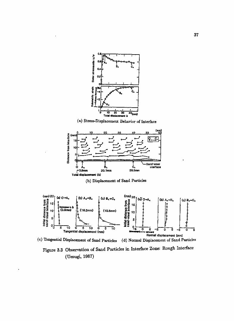
Figure (3.3) shows the details of observations for deformation of sand parti
cles for rough steel-sand interfac~. During various stages of sliding of the interface,
sand particles are tracked by taking photographs through a glass window located
on one of the vertical faces of aluminu~ frame. The sand mass is partitioned
into 8 horizontal layers, (Fig.3.3b). Each layer contains 5 tracked particles. The
displacement of tracked particles are shown in Fig.(3.3b). Open and solid circles
in Fig.{3.3b) indicate the position of sand particles related to the interface dis
placement from point 0 to C4 (Fig.3.3a), respectively. Between 0 to C4 the total
tangential displacement 6 = 39.9 mm whereas the tangential displacement of sand
particles, as seen form Fig.(3.3b), is much smaller than the total displacement.
Figure (3.3c) shows the average and standard deviation of increase in tan
gential displacement of sand particles, whereas Fig.(3.3d) shows the increase in
normal displacement. Here, the 8 open circles on each plot along the height of
interface indicate average displacement of (five) sand particles of each layer, and
the horizontal line passing through the open circle indicates the standard deviation
-i IC,,)
ij-' -@
j j-2 ~JLO.~ ____________ ~
'0 '0 20 30 40 Tot .. cIisoIac~ b Cmrn)
(a) Stress-Displacement Behavior of Interface
o A. 8. r3.9nvn 20.1mm
Total displacement (I)
c. 39.9mrn
(b) Displacement of Sand Particles
37
(mm) 20 (a) O-'A. sB
g-!15 \
Cnvn>20 s B caT ()..A. (b) A.+8. (c) 8.+C.
g~ 10 1a=b .sa;
(16.2mm) (19.8mm)
10
:6~ _I 5 :!l!~ e l1l -en 00 5 10 0 5 10 0 5
Tangential displacement (mm)
( c) Tangential Displacement of Sand Particles
g~ 15 GI.! i~ 10 -;;: '5" 5 3"2 i: O'--.....!--
-5 0 5 -5 0 5 -5 0 5 "-"-UllWW
NonnaJ displacement (mm)
(d) Normal Displacement of Sand Particles
Figure 3.3 Observation of Sand Particles in Interface Zone: Rough Interface
(Uesugi, 1987)

38
of the. displacement of particles of that horizontal layer. From start (0) to peak
(A4) the sand deforms essentially in a uniform manner (Fig.3.3c), and the increase
in volume is small (Fig.3.3d). Between A4 and B4 large tangential displacements
occur near the interface, and associated increase in volume near interface. From
B4 to C4 very large tangential displacements are observed near the interface, but
the volume increase is less than previous stage (A4 to B4). During A4 to C4 there
is large standard deviation in tangential displacements near the interface. This
kind of random movement of particles is typical in a shear zone. In general, shear
zone thickness can be visually identified by observing particle displacements. The
particle displacements in the shear zone exceeds values expected by extrapolating
the displacement due to the shear deformation of sand mass. Also a shear zone is
characterized by large deviation of particle displacement. Based on these arguments
it can be easily conceived that a shear zone is formed within soil mass in the vicinity
of the interface during interface sliding. Observe that during A4 to C4 the value
of ( T /(1) decreases and reaches a steady state, and the volumetric strain (Fig.3.3a)
also reaches a steady value as the point C4 is approached.
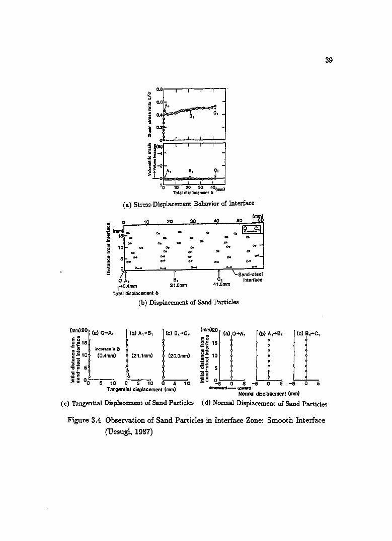
Figure (3.4) shows the details of deformation of sand particles for smooth
interface. The displacement of particles (Fig.3.4b) is much smaller than the total
displacement (8 = 41.4 mm). Evidently the particle displacement in tangential
direction is very small for smooth interface compared with rough interface. Further,
the volumetric increment is negligibly small for the smooth interface.
In summary, along a rough interface, particles slip, roll and move up and
down and the associated tangential and volumetric displacements are large. In
case of smooth interface sand particles slip without large deformations. A shear
zone formation is observed for rough interface and suc..~ formation of shear zone
can be attributed for strain softening behavior associated with volumetric strain
approaching a steady value. Virtually no shear zone formation is observed for
smooth interface.
.8 I I I I
.6 A, J>
.4~ B, C, _
.2
1
) 1 1 1 1
I- -21- -1/' r' r'
-I 1 o 10 20 30 40(mm)
Total displacement b
(a) Stress-Displacement Behavior of Interface
8 o o@ (mm) Go
.!! 15 Go S ... ... ~ ...
CD u e .. li c
......
10 20
Go
Go
co ... ... -..... Go
...
8, 21.5mm
A, rO.4mm
Total displacement b
30
.. Go .. .. ..,. .. ... .....
40
Go .. ... .. ~ ...
C, 41.5mm
Go .. Go
..,. ... .....
"..
Sand-steel interface
(b) Displacement of Sand Particles
Cmm)20 Ca) O"A, (e) B,"C, CD
j~15 CD.!! g.510
Inctaua In b ' (O.4mm) (21.1mm) (20.0mm)
.;: ~Z 5 .!!Ie ~:: °0~-5~-1-0· 0 5 10 0 5
Tangential displacement (mm) 10 ~5 ° 5 -5 0 5 -5 0 5
~MI-upwwd
Normal cisplacement Cmm)
39
( c) Tangential Displacement of Sand Particles (d) Normal Displacement of Sand Particles
Figure 3.4 Observation of Sand Particles in Interface Zone: Smooth Interface
(Uesugi, 1987)

40
3.4 Test Results
Typical test results on monotonic and cyclic loading are presented in this
section in order to study the trend and pattern of the interface behavior. Many
more test results are presented in Chapter 5 along with predictions from the pro
posed interface model. Experimental program is designed in such a way they can
identify the significant factors, namely interface roughness, sand type, mean grain
size (Dso) of sand, initial density Dr and the normal stress. The chosen ranges
for different factors represent actual field conditions. The tests are carried out on
steel-sand and concrete-sand interfaces with various interface roughnesses. The
range of normal stress in the test is 98 - 980 kN/m2 which represents a reason
ably sufficient range for ground-foundation contact surface. In some instances, for
example normal stress in plugs on open-end pile reaches 4 M N 1m2• Thus in the
experiments normal stress range up to 4 MN/m2 is employed. As explained before,
different type of sands with varying Dso are used with initial densities, 90% and
50%.
3.4.1 Monotonic Loading
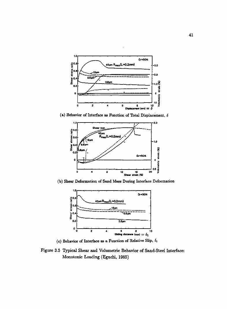
Figure (3.5a) shows shear stress ratio (ria) and volumetric strain as a func
tion of total displacement 6 (= 61 + 62) for steel-Toyoura sand interface. The test
is performed with constant normal stress a = 98 kN 1m2 and the initial relative
density of sand is 90%. In Fig.(3.5b), the curves given in Fig.(3.5a) are presented,
but as a relation with shear strain percentage (62 X 100 / Sand Height). The dashed
line in Fig.(3.5b) indicates the simple shear test results on Toyoura sand. It can be
observed in this figure that the shear stress ratio curves of shear test on Toyoura
sand and the test for interface with roughness 40 p.m virtually coincide. However
the volumetric curves for both cases are some what different. The (r / a) curves
for interface roughness 3.8, 9.6 and 19 p.m fall below the curve of the simple shear
test on Toyoura sand. As seen in Section 3.5.2, this observation is used to define
critical roughness of interface.
ln~------------~~--~------~----.,
-3.0
0,"90" r-8 Q~OIm Rmall(L=O.2mm)
! 0_8 ......... L '91m _ '; ... __ -._-... - - ............ ==::.-:-:.":':--=-==_=_=_=- 1-2.0 :a 0.4 I 9.81m .... 7 -----------------Jl r--... /- 3.81m
0
0•2
/ --------------------
~ 1-1.0-c ~ '; ./-.-_._- - -
o~~======~==========~ o .g D E
'----'---'---------'----'----""'--....... ---'----'--..... 1.0 2 6 8 10 ~
Dlsplac:ement CnwnI = 0 o 2 4
(a) Behavior of Interface as Function of Total Displacement, 6
1.U.--------------~~-------_r~----.,-2.0
Shear tlSt ____ ------::i .g0.8 _-----~ "",*,.. 40..-n " • 0 6 ,f" Rmaa(L=O.2mm> ,'-;. •• 19 " - \ .... ~ ';. / 1.0 ;;;0.4 a.elm / . " ~ " o 3.8 .... ,. ,/
0.2 i- " I " -: ,,'
o~_r..~_-~.-~~----------------------~
o 4 8 12 16 Shear .Ir .... ('5'
(b) Shear Deformation of Sand Mass During Interface Deformation
~O.s ~ 4olmRmu(L=O.2mm) :0.61--. --...;.;--=:..;;;;.......;.:;::..:.:.~ e --___ 191111 0; '---=======:::::::z.:.-=.-.:::.:::.:--=== :au Ulm Jl ~ 0 02 --------------~3~.8~1m=-----------
o~----~--~--~----~~~--------~ o 2 4 8 8 10 Sliding distance (mm) = 01
(c) Behavior of Interface as a Function of Relative Slip, 61
Figure 3.5 Typical Shear and Volumetric Behavior of Sand-Steel Interface:
Monotonic Loading (Eguchi, 1985)
41

42
For the tests shown in Fig.{3.5a), the sliding distance (61 ) is related to (T I u)
in Fig.(3.5c), thus representing the interface behavior. Therefore, in developing the
constitutive relation for the interface, the relation given in Fig.{3.5c) i.e (T I u) VS 61
and the corresponding volumetric strain vs 61 are required for the interface behav
ior.
As can be observed in Fig.(3.5c) that at the begining of interface sliding, the
values of (T I u) reached are very high value for small values of 61. After reaching
the peak value, (T I u) decreases with the increase in 61 , and finally reaches the
residual value. The peak and residual values of ( T I u) are denoted by /-Lp (peak fric
tion coefficient) and /-Lo (residual friction coefficient), respectively. The value of J.Lp
is higher for high interface roughness and the strain softening behavior is predom
inant for rough interfaces. Smooth interfaces cause very small volumetric changes,
whereas higher dilational behavior is observed for rougher interfaces. Moreover,
the dilational volumetric values reach a steady value (Fig.3.5a) with the increase
of 6 (or 01). It is also observed (U esugi, 1987) that sand-concrete interface behaves
essentially the same as sand-steel interface.
3.4.2 Cyclic Loading
Reported tests on cyclic loading are conducted as displacement control tests
by applying total displacement 6 (= 61 + 02) amplitude equal to 4 mm with a
period of 100 seconds up to 15 cycles of loading. Most of the tests are for constant
nonnal stress of 98 kN 1m2 , and in order to study the effect of normal stress on
cyclic loading, another set of tests is performed for u = 490 kN 1m2 • Initial relative
density of sand is 90% for all the tests.
Figure (3.6) presents cyclic test results on smooth and rough steel-Seto sand
interface with u = 98 kNlm2• Only at the begining of the cycle, strain softening
behavior can be noticed for the rough interface. Subsequently, i.e, after reversing
the loading direction, there is no more strain softening effect. For rough interfaces,
the ultimate value of (Tlu) remains essentially the same with the number of cycles
as well as for both positive and negative values of (T I u). This indicates that there

0.8
.2 ~ 0.4 en en e a en
-O.S
Seto Sand t'Oso-o.16nm Uc.1.1
15 -' 2 ( I N=l
~
I . 3.0 .... R .... L.1IO.2mm
-1.0 ,-,.--.,....-..,.....--,---,-..,
ai .... oS e Or-----------~======,,1 en u ;: a; 1.0 § '0 >
2.0 -4 Sliding Distance (mm)
0,
(a) Smooth Interface
. 0.8
.2 ~ 0.4 en en ~ 0 rn ~
CIS
~-o.4 rn
-0.8
Seto Sand N=1 Oso-O.16nmUc·1.1 "",-- 2,00,15
(( ..
" !
; )) ~
. /,9 .... R .... L.=O.2~
(b) Rough Interface
Figure 3.6 Typical Shear and Volumetric Behavior of Sand-Steel Interface: Cyclic Loading (Eguchi, 1985)
43

44
is no significant anisotropic effect on (r / q) due to stress reversal. For smooth
interfaces, the ultimate value of (r / q) increases and then reaches a steady value
with the number of cycles. This is an indication of hardening effect on the ultimate
value of ( r / (j) with the increase of number of cycles.
At the begining of the cycle, dominant dilational behavior prevails and dur
ing unloading and reloading compaction followed by dilation is observed for rough
interfaces. The volumetric loops appear to be very much similar for different cycles.
Interestingly, compaction is taking place with cyclic loading and the net amount
of compaction increases with the number of loading cycles. It is expected that the
compaction reaches a steady value as the number of cycles increases. Such behav
ior is not very obvious in the results presented here as the test is performed for 15
cycles, and this value may not be sufficient to reach the steady value of compaction.
However, for smooth interfaces, Fig.(3.6a), apparently the volumetric compaction
nearly reaches the steady state. As observed, smaller number of loading cycles
are required to reach the steady value of compaction for smooth interfaces than
for rough interfaces. Also the unloading curve is almost parallel to the (r / u) R.'Cis
implying very small elastic displacements after unloading.
Volumetric compaction during stress reversal (unloading and reloading) is
a very important phenomenon in soil mass behavior, that causes liquefaction and
cyclic mobility in saturated sand mass. Interestingly, the same type of volumetric
compaction takes place in the interfaces during cyclic loading.
3.5 Factors Influencing Interface Behavior
It is generally expected that the interface behavior is influenced by type of
sand, mean grain size (Dso) of sand, initial density of sand, interface roughness
and normal stress. Based on experimental results, Uesugi (1987) examined the
significance of possible influence of factors on coefficients of friction (J.lp and J.lo) of
interface using experimental design method. It is important to identify influential
parameters as this will guide one to choose parameters that are used in constitutive
modeling. For this reason, the influential factors are examined in this section.
45
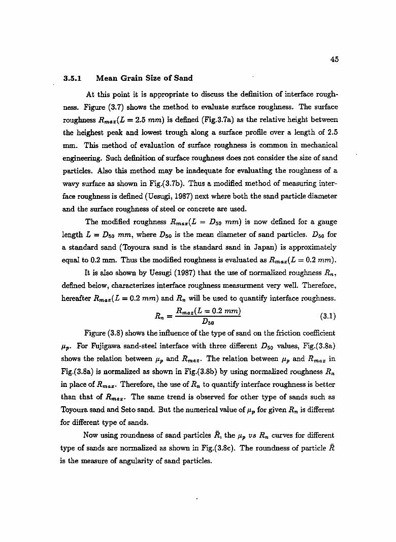
3.5.1 Mean Grain Size of Sand
At this point it is appropriate to discuss the definition of interface rough
ness. Figure (3.7) shows the method to evaluate surface roughness. The surface
roughness Rmu(L = 2.5 mm) is defined (Fig.3.7a) as the relative height between
the heighest peak and lowest trough along a surface profile over a length of 2.5
nun. This method of evaluation of surface. roughness is common in mechanical
engineering. Such definition of surface roughness does not consider the size of sand
particles. Also this method may be inadequate for evaluating the roughness of a
wavy surface as shown in Fig.(3.7b). Thus a modified method of measuring inter
face roughness is defined (Uesugi, 1987) next where both the sand particle diameter
and the surface roughness of steel or concrete are used.
The modified roughness Rmu( L = Dso mm) is now defined for a gauge
length L = Dso mm, where Dso is the mean diameter of sand particles. Dso for
a standard sand (Toyoura sand is the standard sand in Japan) is approximately
equal to 0.2 mm. Thus the modified roughness is evaluated as Rmaz(L = 0.2 mm).
It is also shown by Uesugi (1987) that the use of normalized roughness Rn ,
defined below, characterizes interface roughness measurment very well. Therefore,
hereafter Rma.z(L = 0.2 mm) and Rn will be used to quantify interface roughness.
Rn = Rmaz(L = 0.2 mm) (3.1) Dso
Figure (3.8) shows the influence of the type of sand on the friction coefficient
J.lp. For Fujigawa sand-steel interface with three different Dso values, Fig.(3.8a)
shows the relation between J.lP and Rmaz . The relation between J.lp and Rmaz in
Fig.(3.8a) is normalized as shown in Fig.(3.8b) by using normalized roughness Rn
in place of Rmaz . Therefore, the use of Rn to quantify interface roughness is better
than that of Rmaz. The same trend is observed for other type of sands such as
Toyoura sand and Seto sand. But the numerical value of J.lp for given Rn is different
for different type of sands.
Now using roundness of sand particles R, the J.lP VS Rn curves for different
type of sands are normalized as shown in Fig.(3.8c). The roundness of particle R is the measure of angularity of sand particles.

2.5mm
steel---"r-------J I
Rmax(L=2.5mm) (a) Roughness Measurment: Rmaz(L = 2.5mm)
2Smm 25mm
(a)
(II (2)
(b) Definition of Modified Roughness: Rn
CONCRETE
(a) Rmax==10pm (cab= 131MNm2)
AIR
~ CONCRETE
(b) Rmax==10pm (cab=31MNlm2)
O.2mm ..,.
~! !!mm
( c) Typical Roughness of Concrete Surface
Figure 3.7 Definition of Interface Roughness (Uesugi, 1987)
46

1.0,......-....... ---....--..,.----.---
:::~D .. = XO.,~~.82mm . Pp ~
0.4 '\t A Sym. 050
o 0.16mm
0.2 a 0.54mm
a =98kPa 1.82mm
, o 10 20 30 40 50
Rm .. (L=0.2mm) (11m)
(a) Variation of /Jp with Rm4z(L = O.2mm) :Fujigawa Sand-Steel Interface
1.0
0.6
...!!iQ,o!--: 6 _,.~ /:' .. :b"~ Maximum shear
~ " .. " stress ratio -ff'tJ.' of sand mass
Ibo .. . ~a-, Sym. 0 50
Linear 0 0.16mm
O.S
0.4
0.2 regression a 0.54mm
On-98kPa A 1.S2mm
o 20 40 80 80 100 Rn (10·')
(b) Variation of /Jp with Rn :Fujigawa Sand-Steel Interface
0.25 "X('t/ a )m.. of Toyoura Sand In simple shear tests _;::I!:::~=f
0.20
iix p,
0.15
Selo
Sym. Sand. o Toyoura a Fujlgawa A Seto
00 50 100 150 200 Rn (X10-~)
(c) Variation of R x /Jp with Sand Type
Figure 3.8 Influence of Type of Sands on Interface Behavior (Uesugi, 1987)
47

48
As is seen here, the type of sand plays a major role in the magnitude of /-Lp.
It is also shown that the same influence is observed for the friction coefficient at
residual state /-Lo. The effect of sand type on the volumetric behavior of interface
is not known as data on volumetric behavior is not reported by Uesugi (1987).
3.5.2 Interface Roughness
Observation of Figs.(3.3) to (3.6) and (3.8) indicates that the roughness
plays major role in the interface behavior. Discussion about the effect of interface
roughness can be found in the previous section. Further, one more important effect
of interface roughness will be discussed here by observing Figs.(3.8b,c). Note that
/-Lp is linearly related to Rn in Fig.(3.8b). For Rn greater than approximately
0.07, /-Lp remains constant and this constant value is the maximum stress ratio of
Fujigawa sand in simple shear device.The value Rn = 0.07 is termed as "critical
roughness of interface (R~ri)". From Fig.(3.8c), the critical roughness for Toyoura
sand and Seto sand-steel interfaces is approximately 0.08 and 0.18, respectively.
Here the upper bound of /-Lp is equal to the ultimate friction ratio of sand mass
obtained from simple shear device. From here it follows that when the interface is
smoother than R~ri, interface sliding will take place. On the other hand when the
interface is rougher than R~ri, shear failure occurs in soil mass instead of interface
sliding along the interface. In other words, when the interface roughness is smaller
than R~i, the interface is weaker than the soil mass and vice versa.
The shear strength (in simple shear) of the soil mass defines the critical
roughness of interface. Since the shear strength of the soil mass depends on the
initial density and applied normal stress, it is expected RC;;i will depend on these
factors. It will be clearly shown below how initial density of sand affects the value
of R~ri.
3.5.3 Initial Density
Shown in Fig.(3.9) is the influence of initial density of sand on interface
behavior. For a sand with Dr = 45%, the upper bound value of /-Lp is smaller than

1.0
0.8 p,p
0.6
0.4
0.2
o
I I I I
Maximum shear stress> 6 ratio of dense sand
f- ... 8' Linear ...... 0 . ... regression ~S>
f- ~...... _.-A-·-8· ~ ... A fT
- .......... ~ g
...
I
50 L I
100 150 Rn
Sym. 0
A
DrC%) ==90 ==50
-,
-
..
-
-
Figure 3.9 Influence of Initial Density of Sand on Interface Behavior
(Uesugi, 1987)
49
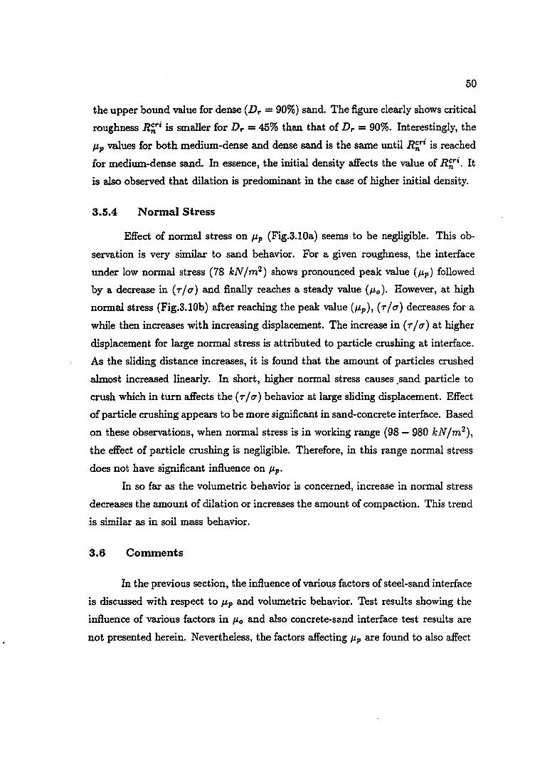
50
the upper bound value for dense (Dr = 90%) sand. The figure clearly shows critical
roughness R~ri is smaller for Dr = 45% than that of Dr = 90%. Interestingly, the
Jlp values for both medium-dense and dense sand is the same until R~ri is reached
for medium-dense sand. In essence, the initial density affects the value of R~ri. It
is also observed that dilation is predominant in the case of higher initial density.
3.5.4 Normal Stress
Effect of normal stress on Jlp (Fig.3.lOa) seems to be negligible. This ob
servation is very similar to sand behavior. For a given roughness, the interface
under low normal stress (78 kN/m2 ) shows pronounced peak value (f1.p ) followed
by a decrease in (T/q) and finally reaches a steady value (Jlo). However, at high
normal stress (Fig.3.l0b) after reaching the peak value (Jlp), (T/q) decreases for a
while then increases with increasing displacement. The increase in (T / q) at higher
displacement for large normal stress is attributed to particle crushing at interface.
As the sliding distance increases, it is found that the amount of particles crushed
almost increased linearly. In short, higher normal stress causes ,sand particle to
crush which in turn affects the (T/q) behavior at large sliding displacement. Effect
of particle crushing appears to be more significant in sand-concrete interface. Based
on these observations, when normal stress is in working range (98 - 980 kN/m2 ),
the effect of particle crushing is negligible. Therefore, in this range normal stress
does not have significant influence on J1.p.
In so far as the volumetric behavior is concerned, increase in normal stress
decreases the amount of dilation or increases the amount of compaction. This trend
is similar as in soil mass behavior.
3.6 Comments
In the previous section, the influence of various factors of steel-sand interface
is discussed with respect to Jlp and volumetric behavior. Test results showing the
influence of various factors in J1.o and also concrete-saud interface test results are
not presented herein. Nevertheless, the factors affecting J1.P are found to also affect
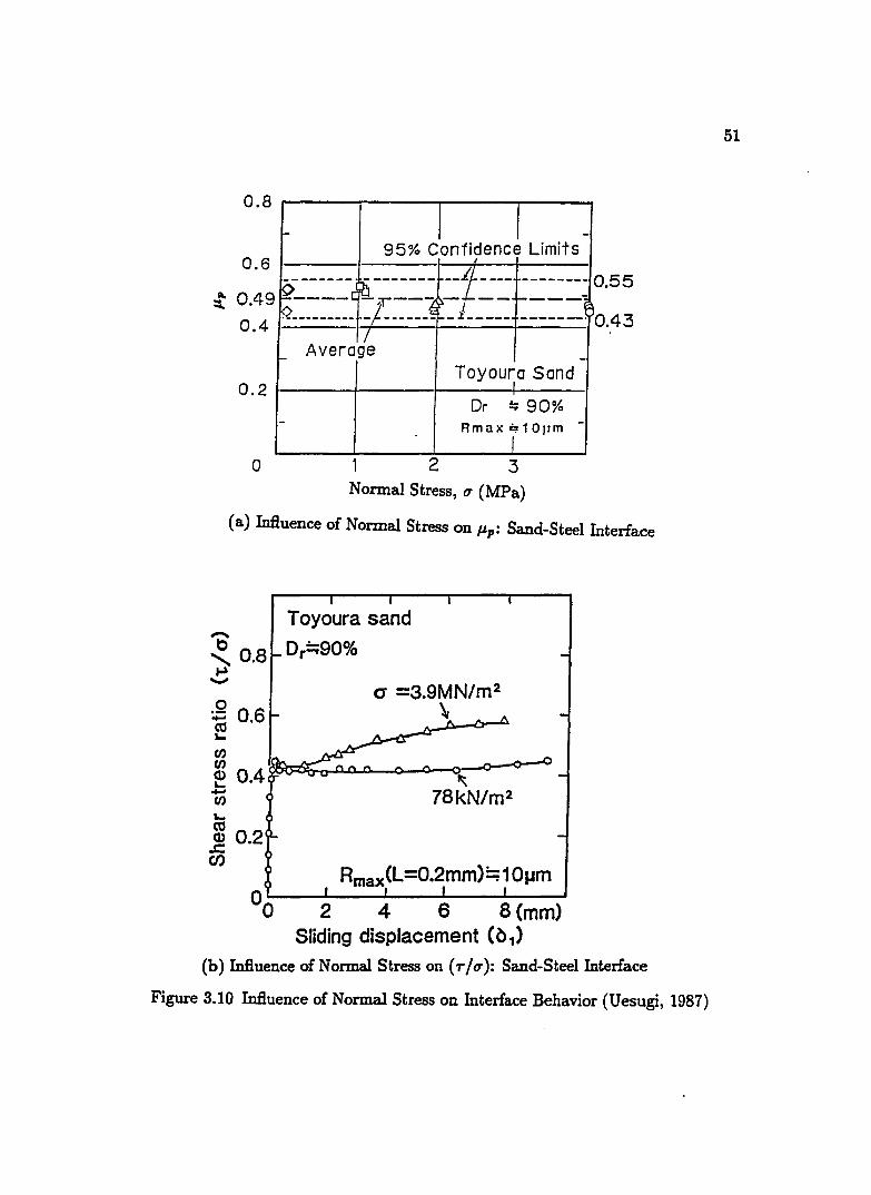
0.8
0.6
::t 0.49
0.4
0.2
o
- I I L' 't -95% Confidence Iml 5 /
~------.
fi~~==~ -~t.------------
F----C ?-- -- ~---j
~---------~ _L ____ ------- 0.43
0.55
- Average -Toyou~a Sand
Dr !; 90% - RmnXj10 p m -
2 3 Normal Stress, u (MPa)
(a) Infiuence of Normal Stress on IJp: Sand-Steel Interface
Toyoura sand -t:) 0 8 0 r~90% ,. ~ - a =3.9MN/m2
\
Rmax(L=O.2mm)" .1 Opm
2 4 6 8 (mm) Sliding displacement (b 1)
(b) Infiuence of Normal Stress on (T/q): Sand-Steel Interface
Figure 3.10 Influence of Normal Stress on Interface Behavior (Uesugi, 1987)
51

52
the values of J.lo in the same manner as of J.lP' though the numerical magnitude of
J.lP and J.lo are different (Uesugi, 1987). It is also noticed that the characteristics of
concrete-sand interface are essentially similar to those of the steel-sand interface.
Therefore, the discussion about the influencing factors for steel-sand interface is
also valid for the case of concrete-sand interface~
Influence of various factors are discussed both qualitatively and quantita
tively for J.lP and J1.o, and only qualitatively for volumetric behavior. In general,
developement of an elasto-plastic constitutive model requires the input of the entire
( T / (j) us 51 and volume us 51 curves, and not just certain points on these curves.
Since the influencing parameters are connected to some important strategic points
(J.lp and J.lo) of stress-strain curves, this discussion provides insight and guidance
to choose proper variables necessary to define constitutive relations for interface
behavior.

CHAPTER 4
FORMULATION OF CONSTITUTIVE RELATION FOR
INTERFACE
4.1 Introd uction to Hierarchical Approach of Modeling
53
This chapter presents the details of approach followed in the hierarchical
manner to develop an elasto-plasticity based constitutive relation for interface be
havior. The attractiveness of plasticity theory stems from its capability to model
many essential material characteristics, namely: any type of complicated stress
strain paths, anisotropy and cyclic mobility, with sufficient accuracy. However,
constitutive relations developed to cover a wide variety of material behavior under
diverse loading conditions tend to be either so general that they cannot yield spe
cific needed information, or they become too complicated t.o be of practical use.
Therefore, it is both natural and necessary to attempt to develop models for specific
classes of materials under specific loading conditions, simple constitutive descrip
tions which capture the essential physical features of problem. Thus a sucessful
constitutive model should have the following characteristics.
(1) Model applicability for wide range.
(2) Accuracy achieved in terms of number of input data and measurment of
these data.
(3) Easy to adopt in the solution of numerical problems.
It is therefore important that a model should be formulated in a "modular way"
(Desai and Siriwardane, 1984; Mroz and Norris, 1982), that is, allowing for neglect
or considerations of some effects without affecting other assumptions, or identified
material parameters. In order to obtain such modular forms of model, a basic
model describing simple features is modified by introducing different features one
at a time in a hierarchical manner to model, in an improved way, the real behavior

54
of a material. In other words simplicity of the original model is preserved with
modification being introduced progressively to model "rising complexity of the phe
nomena. The process of adding an additional feature (complexity) to a certain
modular form of model is termed "hierarchical approach of modeling" (Desai et
al.,1986).
The hierarchical approach used for the modeling of soils and rock joints by
Desai et al., 1986; Frantziskonis and Desai, 1987; Somasundaram and Desai, 1988;
Fishman, 1988; Desai and Fishman, 1988, is adopted here. A generalized three
dimensional plasticity model capable of predicting the behavior of solids such as
soil and rock is specialized by Desai and Fishman (1988) and Fishman (1988) to
describe the behavior of individual rock joints. Here, using the analogy between
various quantities in solids and joints, the yield and plastic potential functions for
rock joints are obtained.
In this study, the yield and potential functions proposed by Desai and Fish
man (1988), and Fishman (1988) for rock joints are adopted to model the interface
behavior. The remaining part of this chapter contains the details of the proposed
elasto-plasticity model for the interface developed using the hierarchical approach
of modeling i.e starting with a simple model (associative model with isotropic
hardening) how modification is introduced hierarchically to obtain a model having
non-associativeness, strain-softening effect and cyclic loading capability. First, the
idealization of the interface is presented. Then, the proposed elasto-plasticity model
for the interface under monotonic loading is discussed. Subsequently, extension of
the model to the cyclic behavior of the interface is presented. Next, the functions
(a, OlQ and r) required to define the model are presented. Finally, the constitutive
relation for the interface in terms of incremental force and displacement is derived.
4.2 Mathematical Idealization of Interface
An idealization of an interface between two contacting bodies A and B is
shown in Fig.(4.1). During stress transfer from body A to body B or vice versa,
very often relative slip takes place along the interface plane. Such tendency of
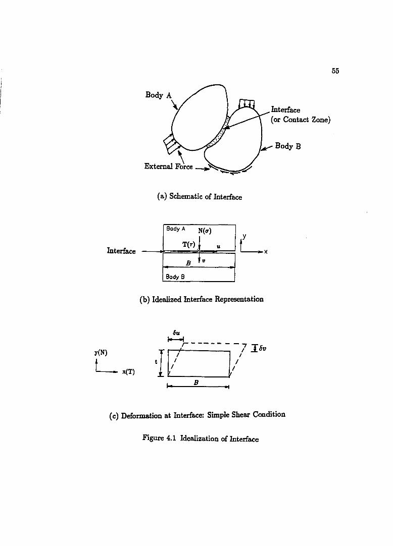
Interface
yeN)
L x(T)
( a) Schematic of Interface
Body A N(cr)
T(r) J u
B tv
Body B
(b) Idealized Interface Representation
6u 1--1 r-------
'1[/ ~/ I6v
I B
Interface (or Contact Zone)
( c) Deformation at Interface: Simple Shear Condition
Figure 4.1 Idealization of Interface
55
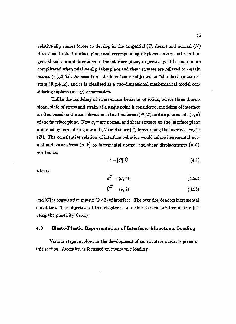
56
relative slip causes forces to develop in the tangential (T, shear) and normal (N)
directions to the interface plane and corresponding displacements u and v in tan
gential and normal directions to the interface plane, respectively. It becomes more
complicated when relative slip takes place and shear stresses are relieved to certain
extent (Fig.3.5c). As seen here, the interface is subjected to "simple shear stress"
state (Fig.4.1c), and it is idealized as a two-dimensional mathematical model con
sidering inplane (x - y) deformation.
Unlike the modeling of stress-strain behavior of solids, where three dimen
sional state of stress and strain at a single point is considered, modeling of interface
is often based on the consideration of traction forces (N, T) and displacements (v, u)
of the interface plane. Now q, T are normal and shear stresses on the interface plane
obtained by normalizing normal (N) and shear (T) forces using the interface length
(B). The constitutive relation of interface behavior would relate incremental nor
mal and shear stress (I;, f) to incremental normal and shear displacements (v, 'Ii ) written as;
where,
itT = (I;,f)
U· T ( •. ) _ = V,u
(4.1)
( 4.2a)
( 4.2b)
and [C) is constitutive matrix (2 x 2) of interface. The over dot denotes incremental
quantities. The objective of this chapter is to define the constitutive matrix [C)
using the plasticity theory.
4.3 Elasto-Plastic Representation of Interface: Monotonic Loading
Various steps involved in the development of constitutive model is given in
this section. Attention is focussed on monotonic loading.

57
4.3.1 Elastic Behavior
The incremental elastic behavior of interface is expressed as;
(4.3a)
or
(4.3b)
where, [ee] is the elastic constitutive matrix of interface and K n and K" represent
elastic normal and shear stiffness of interface. In postulating Eq.( 4.3), it is assumed
that elastic normal and shear behavior is uncoupled. Such an assumption not only
yields a less complicated model but also reduces the required number of material
parameters.
4.3.2 Plastic Behavior
It is assumed that the interface behavior is rate independent i.e natural time
scale does not enter in the constitutive relationship. Also the constitutive matrix
[e] in Eq.(4.1) depends on stress, displacement and hardening (plastic) parameters
not on q and V. In the context of the plasticity theory, the following conditions are assumed;
(1) There exists an yield (or loading) surface separating ( a) the loading process
associated with the generation of plastic strains and (b) unloading process (or
reverse loading). In the stress space, such yield surface is defined as
f(q,g) = 0 (4.4)
where, q and ~ represent stress vector and vector of state or hardening (plastic)
parameter.
(2) Incremental displacement vector is decomposed into elastic and plastic part as;
(4.5)
The superscripts e and p denote elastic and plastic parts, respectively.
(3) According to classical plasticity, when incremental stress vector q is directed
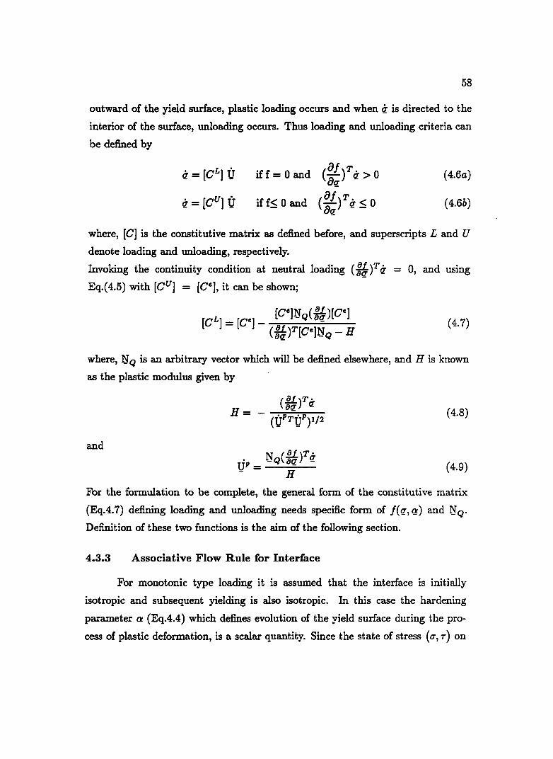
58
outward of the yield surface, plastic loading occurs and when q is directed to the
interior of the surface, unloading occurs. Thus loading and unloading criteria can
be defined by
q = [CLp)
q = [Cu)1)
iff = 0 and
iff~ 0 and
(4.6a)
( 4.6b)
where, [C] is the constitutive matrix as defined before, and superscripts L and U
denote loading and unloading, respectively.
Invoking the continuity condition at neutral loading (U f q = 0, and using
Eq.( 4.5) with [CU] = [Ce], it can be shown;
(4.7)
where, N Q is an arbitrary vector which will be defined elsewhere, and H is known
as the plastic modulus given by
H= (!!L)T if au -
(4.8)
and
(4.9)
For the formulation to be complete, the general form of the constitutive matrix
(Eq.4.7) defining loading and unloading needs specific form of f(q, q) and NQ •
Definition of these two functions is the aim of the following section.
4.3.3 Associative Flow Rule for Interface
For monotonic type loading it is assumed that the interface is initially
isotropic and subsequent yielding is also isotropic. In this case the hardening
parameter a (EqAA) which defines evolution of the yield surface during the pro
cess of plastic deformation, is a scalar quantity. Since the state of stress (u, T) on

59
the interface plane influences the yielding characteristics of the interface, the yield
function for interface can take the following fonn;
f(q, T, Q) = 0 (4.10)
Identifying the analogy between (J1!J2D) in solids (Appendix A) and (q,T) in
joints, Fishman and Desai (1987), Desai and Fishman (1987), Fishman (1988),
and Desai and Fishman (1988) used the following yield function for the joints;
(4.11)
Equation (4.11) is used as yield function for the interfaces and, here, and n are
interface parameters. Figure (4.2) shows the family of typical yield curves given
by Eq.(4.11) for rough and smooth interfaces. Evolution of the yield function is
due to hardening parameter Q. Definition of Q is given elsewhere. Parameter n is
called phase change parameter as it defines the state where volume changes from
contraction to dilation. The shape of the yield function is governed primarily by n.
For n = 2, the yield function gives a set of straight lines or cone shape in (q - T)
space. As n increases beyond 2, the yield surface will fonn a closed surface with
large curvature.
Postulation of Eq.( 4.11) is the consequence of the assumption that T in the
direction (x) of shear displacement contributes to the yielding of interface, whereas
the influence of other shear stresses which are oriented in the direction perpendic
ular to interface plane (x, y) is disregarded. This assumption is compatible with
two-dimensional (x, y) idealization of interface. One has to keep in mind that be
c?.use of isotropic shear behavior of interfaces, one and only one stress path such as
forward loading (positive x direction) or backward loading (negative x direction)
is possible during interface deformation. Thus stress path does not play a role in
interface behavior. Now, associative flow rule is obtained by defining
N = (of) -Q oq (4.12)
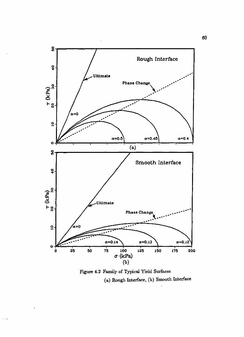
~~------------~------------------------------~
o •
o "';'M c.. e 1-0
N
o ...
Rough Interface
.... .. .... ....
Phase Change ........ \ ............ .. ..
...... ....
a=O.4-
o~----~----~----~----~----~----~----~----~ (a)
~,-----------------------~~------------------~
o •
o ...
Smooth Interface
Phase Chan .. e ......... .. .. \ .. .. -....
..... ." ... -...
O~~--~----~----~I~--~~----~----~----~--~ a 2~ ~o 7~ 100 12~ l~O 17~ 200
a (kPa) (b)
Figure 4.2 Family of Typical Yield Surfaces
( a) Rough Interface, (b) Smooth Interface
60
61
4.3.4 Non-Associative Flow Rule for Interface
The necessity to use 'non-associative How rule to represent volumetric be
havior for geologic materials is very well documented in literature. In general
associative How rule would predict stress behavior accurately but it fails to predict
volumetric (stress induced) behavior accurately. Often associative How rule results
in predicting too large volume expansion. This is due to the assumption that the
incremental plastic strain vector is normal to yield surface. However experimen
tal evidence shows soils exhibit deviatoric normality, i.e in octahedral plane the
deviatoric components of incremental plastic strain vector is normal to projection
of yield surface on that plane (Baker and Desai, 1982). Consequence of devia
toric normality is that a plastic potential function Q can be obtained by adding a
function h (u, e) to the yield function as (Desai et al., 1986);
Q = f(u,r,Ci) + h(u, e) i: 0 (4.13)
Observe that the function h depends on the normal stress u and a measure of
plastic strain accumulation e. An alternative explanation for Eq.( 4.13) is that the
volumetric strain is associated with normal stress u, and a modification in the u
term. in yield function should be thought to give better prediction for volumetric
behavior.
It is assumed that the non-associative characteristics of interface is same as that of geologic materials. Hence, based on the above evidence, a simple function
for Q is proposed below by replacing Ci in Eq.( 4.11) by CiQ (Fishman, 1988);
(4.14)
The parameter CiQ plays paramount role in defining normal displacement of in
terface (Navayogarajah, 1988). In general CiQ depends, among various factors, on
Ci and state of stress. Further detail of CiQ is given in Section 4.5.1. The plastic
potential surface Q, given by Eq.( 4.14), does not coincide with yield surfaces. But
the shape of Q surfaces are similar to that of yield surfaces and for non-associative
62
flow rule' the two family surfaces cross each other. Non-associative flow rule is
obtained by setting;
(4.15)
Setting o:q = 0: results in Q = f = 0 or associative flow rule. This procedure
explains the evolution of non-associative model from associative model in the hier
archical manner.
4.3.5 Modeling of Strain Softening Behavior
During monotonic type loading, strain softening and shear band or shear
zone formation is very predominant for a rough interface while a smooth interface
does not exhibit such behavior (Yoshimi and Kisida, 1981; Uesugi, 1987). At given
nonnal stress, after reaching the peak value, the shear stress T decreases during the
process of softening. Also the rate of volumetric strain (dilation) diminishes and
volume curve approaches a finite value (Section 3.4.1). Relevant mathematical pre
liminary to include these aspects in the modeling is presented in this section. The
concept of decomposition of material behavior (Fig.4.3) to model strain softening
response of concrete and soil used by Desai, 1974; Desai et al., 1986; Frantziskonis
and Desai, 1987, is adopted here to model the strain softening behavior of the
interface.
The observed or average response (stress) of interface is assumed to be sum
of response of two parts namely (1) intact (or topical) part and (2) damaged part as
shown in Fig.( 4.3). During shear loading, intact part is progressively transformed
into damaged part due to accumulation of (plastic) strains. Characterization of the
intact part and damaged part is achieved by elasto-plasticity and rigid-plasticity,
respectively. Thus, the non-associative model presented in Section 4.3.4 is applica
ble for the intact part. It is assumed the shear strength of damage part is zero, but
it can sustain normal stress. Thus, it is assumed the normal stress is not affected
by the damage and normal stress should be compressive. With these assumptions,
the observed or average interface stress can be written as;

F
(a) Representation of Component Areas and Forces of
a Partially Damage Body
Shear Stress
Stress Relieved Behavior
Strain
(b) Concept of Decomposition of Material Behavior
Figure 4.3 Strain-Softening Behavior (Frantziskonis and Desai, 1987)
63
or
{ ~ } = (1- r) { ~: } + r { ~t }
{ ~ } = { (1 ~~ )r' }
64
(4.16a)
(4.16b)
The parameter r = (Ao/A) is a scalar quantifying the damage. Here, Ao is the area
of damaged part and A is the total area (FigA.3). In Eq.( 4.16) the state of stress
vectors {O', r}, {O't, rt} and {O't, O} relate to average, intact part and damaged part of
the interface, respectively. Inspection of Eq.( 4.16) shows that 0' = (7t, r = (1- r )rt,
thus the normal stress is not affected by damage, only shear stress is affected. This
observation is compatible with the assumptions.
It is assumed that there is no relative movement between intact part and
damaged part. Thus, the interface displacement vector {v, u}, i.e the average be
havior, is same in the intact part and damaged part.
{v,u} = {v'U}intact part = (V,U}damaged part (4.17)
Differentiation of Eq.( 4.16) yields
(4.18)
At the end of this chapter, it is shown that r can be expressed as
(4.19)
As explained before, the behavior of intact part can be expressed using
Eq.(4.7) with the non-associative flow rule. Combining Eqs. (4.7), (4.15), (4.18)
and (4.19), the observed or average interface behavior is expressed as
q = [Cep*] (J ( 4.20)
The matrix [Cep*] is the constitutive matrix of average behavior of interface and
is given by;
(4.21)

65
Again, examination of Eq.( 4.21) indicates that the normal stress is not changed,
only the shear stress is changed due to the strain softening effect. Setting r = 0
(no softening effect) reduces Eq.(4.21) into Eq.(4.7), and this idicates how softening
effect is incorporated on non-associative model in hierarchical order.
4.4 Extension of Model to Cyclic Loading
4.4.1 Introduction to the Important Aspects of Cyclic Loading
In contrast to monotonic loading where only unidirectional loading takes
place, cyclic loading involves the reversal of stress direction. Thus, cyclic loading
has combination of different loading phases namely; loading, unloading, reloading
and reverse loading. Such loading phases make modeling of cyclic loading more
complex than monotonic type loading.
Desai and Fishman (1988), Fishman (1988) and Zubelewicz et al. (1987)
presented plasticity models for cyclic behavior of rock joints. When soil is subjected
to cyclic loading, it has been observed (1) plastic strains are developed during both
unloading and reioading, (2) existence of hysteresis loop, (3) volumetric strain
(plastic) developed during unloading is compressive and cyclic volumetric strain
reaches a stable state as the number of loading cycles increases, and (4) stress
reversal point and the strains at the commencement of unloading play an important
role in the unloading and reloading behavior. Observation on cyclic volumetric
behavior of the interface (Section 3.4.2), particularly cyclic compaction, is some
what similar to the behavior of soil under cyclic loading rather than to rock joint
behavior.
In the classical plasticity theory, the yield surface from where unloading
starts is kept in material memory. IT the stress state falls within the memory sur
face, elastic strains are developed and when stress state crosses the memory surface,
plastic (and elastic) strains are developed. This shows that the classical plastic
ity can not simulate plastic strains developed during the unloading and reloading
phases. Therefore, it is evident the concept of yield surface and material memory
as defined in classical plasticity theory has to be modified in order to have plastic

66
strains developed during unloading, reloading and reverse loading phases. The fol
lowing section deals with the development of constitutive relations for an interface
subjected to cyclic loading.
4.4.2 Proposed Method to Include Cyclic Loading Behavior
The development of a simple constitutive model based on limited number
of test data on cyclic behavior of interface is presented in this section. An attempt
is made to faithfully model very important aspect of cyclic behavior of interfaces
such as densification during cyclic loading, plastic strain development during re
verse loading and to some extent induced anisotropy due to rearrangement of soil
particles under stress reversal.
The framework of the basic interface model for monotonic loading is modified
in order to model cyclic behavior. This implies the hierarchical nature involved in
developing a constitutive model for cyclic behavior of interface. The interface model
for monotonic loading is essentially isotropic hardening, thus implying the proposed
model is also isotropic hardening. Such isotropic hardening models fail to produce
some of the important features of cyclic loading such as permanent densification
and hysteresis (Zienkiewicz et aI., 1985). Though the proposed cyclic interface
model is based on isotropic hardening, the following features of the proposed model
makes it anisotropic to some extent, and allows it to incorporate cyclic behavior
of interfaces: (1) effect of change of loading (shear) direction (from forward to
backward or vice versa), (2) proper definition of material memory, and (3) use of
a new cyclic parameter in aq.
4.4.2.1 Definition of Material Memory
First, the definition of loading, unloading, reloading and reverse loading is
presented. Then, the material memory for the interface is defined.
Figure (4.4) shows typical stress path followed by interface in (0', T) space.
Let point A be the initial state of stress and OA' A is the corresponding initial yield
surface. Consider a stress path ABeD. When stress point moves from A to B,
the initial yield surface OA' A gradually evolves into yield surface OBB' which

67
T
o Backward
(or Negative r)
1 Image of Surface OBB'
Figure 4.4 Schematic of Various Stress Paths During Cyclic Loading

68
passes through point B. The stress path AB indicates loading phase. The path BC
moves inward from the yield surface OBB', thus this path represents unloading.
The path CD is known as reloading as this path moves towards the previous
yield surface OBB' but lies within this yield surface. Now consider another stress
path ABCEFGH. As noted before, paths AB and BCE represent loading and
unloading phases. The path CE crosses u axis at E, and enters the backward phase
(r negative) and reaches point F, and OFHH' is the new yield surface. The stress
path EF is known as reverse loading. Again paths FG and GH represent unloading
and reloading, respectively. Obviously, reverse loading indicates the change of r
from !orward (r positive) to backward (r negative) phases or vice versa. Next
material memory surface is defined for the interface.
It is assumed that unloading and reloading do not cause plastic strains,
thus these two loading cases will generate only elastic strains. Elastic unloading
and reloading implies no hysteresis loop. However, available test data (Uesugi,
1987) indicates very small hysteresis loops at small strains and almost no hysteresis
loop at large strains during one-way cyclic loading. This observation justifies the
assumption that elastic unloading and reloading do not involve significant plastic
strains.
During the stress path ABCD (Fig.4.4), stress reversal takes place at point
B and since stress path BCD lies within the yield surface OBB', this yield surface
represents the latest yield surface for the stress path in question. Therefore, the
yield surface OBB' represents material memory surface during the unloading and
reloading phases of paths BC and CD. According to the assumption, only elastic
strains are generated during the paths BC and CD.
Each time whenever stress path changes from forward phase to backward
phase or vice versa, the previous material memory fades away or previous history
is disregarded, and the starting conditions are reinitialized. For example, during
the path ABCEFGH, the yield surface OBB' is the memory surface for the paths
BC and CEo When the stress path CE changes from forward to backward phase
(or crosses (1 axis) at point E and moving towards F, the memory surface OBB'
is erased from the material memory. During stress path EF, a new set of yield

69
surfaces are invoked; initial yield surface 0 E' E and current yield surface OF H H' .
This means that during the reverse loading path EF, plastic strains are generated.
Now, the yield surface OFHH' is the memory surface during the paths FG and
G H, thus no plastic strains are generated during these two stress paths. In essence,
two sets of families of yield surface exist; one set above (1 axis (forward phase) and
the other set below (1 axis (backward phase). When the stress point is in forward
phase, the set of yield surfaces belong to forward pass is invoked and the material
will not remember previous (backward pass) set of yield surfaces.
The assumption of two sets of yield surfaces has very different consequences
in the formulation presented here and conventional plasticity theory. In conven
tional plasticity, for isotropic hardening type models, the zone enclosed by the yield
surface OBB' (Fig.4.4) and its mirror image surface OBIt B' (dotted line) about
(1 axis is purely elastic. Therefore, reverse loading path EF, as it falls within the
elastic zone enclosed by surface 0 B" B', will give only elastic strain not plastic
strain as proposed herein.
4.4.2.2 Definition of Cyclic Parameter
A cyclic parameter n is introduced in plastic potential function D:Q such
that this parameter will introduce non-associative flow rule whenever stress path
changes from forward to backward phase or vice versa. The parameter n controls
the amount of compaction during the reverse loading phase.
During monotonic loading, when there is no shear and the interface is sub
jected to only normal load, it is assumed the interfaces obey the associative flow
rule (Section 4.3.4). Non-associativeness begins only with the presence of shear
stress on the interface. However, introduction of parameter n in D:Q during cyclic
loading initializes non-associativeness even in the absence of the shear force. This
implies that the interface is not isotropic under normal load during cyclic loading.
This phenomenon can be explained from a physical point of view; due to particle
rearrangement, the interface can exhibit anisotropic effects during cyclic loading.
Hence inclusion of parameter n is based on physical reasoning, moreover, it can
capture anisotropic effect in the mQdel during cyclic loading.

70
4.4.2.3 EfFect of Displacement Amplitude
One more assumption about material memory is necessary in order to rep
resent the effect of small and large displacement amplitudes for two-way cyclic
loading. Figure (4.5) shows the effect of displacement amplitude on the inter
face behavior under constant normal stress. At small displacement amplitudes
(FigA.5a), the peak value of ( T / u) in hysteresis loops increases with number of cy
cles untill (T / q) reaches the maximum value. After reaching the maximum value,
( T / q) decreases with the number of cycles and finally reaches a steady value at
larger number of cycles. Interestingly, the maximum and steady value of ( T / q) are
apparently the same as those of peak (pp) and residual (Po) friction coefficients
during monotonic loading (Uesugi, 1987). On the other hand, for large displace
ment amplitudes (Fig.4.5b), which is sufficient enough to bring the interface in
strain-softening region, the shear stress shows strain-softening behavior during the
start of the cycle. After the very first load reversal, the peak shear stress ratio al-
. ways takes a value equal to residual friction coefficient (Po) of monotonic loading,
and no strain-softening behavior is observed.
In order to represent the effect of displacement amplitudes, it is assumed
that the loading phase of the first cycle will assume the stress-strain behavior of
monotonic loading OABCD (Fig.4.5c). This assumption enables one to include
strain-softening behavior during loading phase of first cycle for large displacement
amplitude. It is also assumed that the subsequent cycles of stress-strain behavior
will be decided by the position of stress reversal point with respect to peak shear
stress Tp (Fig.4.5c) in the following manner. Suppose the stress reversal takes
place at a point before reaching Tp , for example at point A, then AX represents
unloading and the shape of the reloading path XY Z is assumed to be same as that
of monotonic path OABCD. While moving on the reverse loading path XYZ, if
stress reversal takes place at a point which has not yet reached Tp , then the above
sequence will be followed during a two-way cyclic loading.
In the process of cycling, now consider that for the first time stress reversal
point reaches the value of Tp or falls within the strain-softening region; for example

71
,,/(1 1'/(1 1'/~ Cycle (ydl ~jrnber.2, 15
o.e /UIIW 0.. cell' 1 , .. , ,.". S(If" f . -31 . -40 70
·41 ·42 100'" 4S 44'" .,:. U
J 0.. 0..
( a) Displacement Amplitude: Small
(Uesugi, 1987)
(b) Displacement Amplitude: Large
(Uesugi, 1987)
1'p
Monotonic Loading Curve
Forward
T
Stress Reversal Point
/~C D
----------~~~--~--~----+_--~~u
Backward o x P
( c) Mechanics of Model to Consider Effect of
Displacement Amplitude
Figure 4.5 Effect of Displacement Amplitude on Cyclic Loading

72
stress reversal takes place at point C (Fig.4.5c). In this case it is assumed that
the reverse loading path PQ R and all the subsequent reverse loading paths would
not show strain-softening effect. In other words, when a stress reversal point falls
within the strain-softening region, it is postulated that the subsequent loading
events will not exhibit strain-softening behavior. As depicted in Fig. ( 4.5c), reverse
loading path PQR will not exhibit strain-softening behavior, and shear stress T
will reach a maximum value equal to the value of Tr of monotonic loading case.
The merit of this postulate is demonstrated in Chapter 5.
4.5 General Functions for a, aQ and r
Since rough interfaces exhibit stable behavior despite dilatancy, it may be
expected that besides volumetric hardening, there is an additional hardening effect
due to shear action. Notice that in the case of interface, magnitude of volumet
ric or vertical displacement is much smaller than that of the shear displacement.
Combination of volumetric and shear deformations, and interface roughness Rn
can contribute to hardening, hence the hardening function a can be expressed as
( 4.22)
where, ev = J IdvPI and eD = J IduPI are the plastic displacement trajectories.
The asymptotic nature of the failure condition during monotonic loading requires
hardening function to approach zero asymptotically with increasing values of ev and eD during defonnation. A set of test data, with every other condition similar
except interface roughness, show the rate of change of a with respect to eD increases
with increase of interface roughness.
The evolution function Qq defines the potential function Q , thus influencing
volumetric behavior of interface. At large shear displacements, it is observed that
the rate of dilation diminishes and the volumetric curve approaches a finite value.
Hence Qq can be a function of the damage parameter r. Based on this evidence
QQ can be expressed as
( 4.23)

73
It is found that eD is a convenient parameter to measure degree of damage r
(Frantziskonis and Desai, 1987). Since interface roughness plays major role in the
strain-softening behavior, r can be represented bYi
(4.24)
4.5.1 Definition of Interface Roughness Ratio R
A new parameter R is defined below to quantify the measure of relative
roughness of interface. The normalized interface roughness Rn can be replaced by
a convenient parameter termed hereafter as "interface roughness ratio R ". The
interface roughness ratio R is defined as;
if if
Rcri > R n n Rcri < R n - n
(4.25)
The critical roughness R;ri is defined in Section 3.5.2. Numerically, R varies from 0
to 1, and it is a non-dimensional quantity. For this reason, R can be used as a state
variable in the constitutive equation in place of Rn. Note the similarity between
the initial relative density Dr (0% ~ Dr ~ 100%) and Rj Dr is a parameter that
reflects the measure of relative density of soil mass. In the same manner, R reflects
the measure of relative roughness of the interface.
The choice of specific functions for a, aQ and r is very important as these
functions control the quantitative as well as qualitative predictive capability of
model. It follows that the choice of these functions should be guided by experi
mental evidence as well as theoretical requirements.
4.5.2 a, aQ and r for Monotonic Loading
A monotonically decreasing function for a is proposed as
(4.26)
Here 'Y is ultimate (or failure) parameter and a, b are material parameters. 'Y
depends on interface roughness ratio R. The parameters a, b are positive quantities
and in general depend on R .
74
The theoretical (or exact) expression for cxQ, can be derived using the flow
rule (Eq.4.40), is given as
cxQ = (-)- ('Y - cxuR 2)1/2(_) + 'Y 2 1 [ _ dvP ]
n 0'0-2 dup (4.27)
By feeding experimental data to the right hand side of Eq.( 4.27), one can obtain
the observed (or experimental) value of CXQ. Such observed variation of CXQ for
three interface roughnesses obtained from the test data in Fig.(3.5) is shown in
Fig. (4.6).
Now the following expression is proposed for cxQ
( 4.28)
Here K. is a material parameter that defines the slope of vertical displacement curve
at the point where shear stress T reaches its peak value. Since the slope of vertical
displacement curve at T = Tp varies with the interface roughness ratio R , the
parameter K. depends on R. The damage parameters r and ru in Eq.(4.28) are
defined later. The value of cx at phase change point (the point where change of
vertical displacement is zero) for the associative flow case (J = Q = 0) is defined
as CXph in Eq.( 4.28). The magnitude of CXph is obtained, by solving -U = 0 for cx ,
as
(4.29)
The CXi is defined as the value of cx at the initiation of non-associativeness. For
an isotropic interface under normal stress, non-associativeness starts when the ap
plication of shear stress starts. By this definition, for a shear test, CXi takes the
value
(4.30)
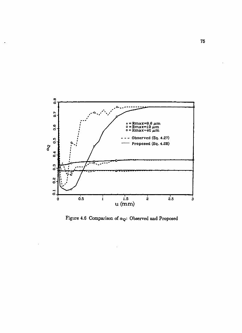
CD ei
l"-ei
CD ei
It')
0 r::t ~ • 0
M 0
N 0
... 0
0
, , , , , , , , , ~, ... ,
0.5
, ,
. ,. , • .0. .. ,,' '",'
1
~O __ .--.--·---~-'--------------------4
6 = Rmax=9.6 J.'m c = Rmax=19 J.'m o = Rmax=40 J.'m
Observed (Eq. 4.27)
Proposed (Eq. 4.28)
Qi_. __ _
1.5 u(mm)
2 2.5 3
Figure 4.6 Comparison of aQ: Observed and Proposed
75

76
The factor [1-11':(1-:")] is known as non-associative parameter. Setting this factor
equal to zero in Eq.( 4.28), one gets o:q = 0: i.e associative Bow rule. Equation (4.28)
for o:q is postulated by equating o:q in Eq.( 4.28) to the theoretical value (Eq.4.27)
at strategic points such as
(1) initiation of non-associativeness,
(2) phase change point,
(3) T = Tp and
(4) T = Tr •
Before the initiation of non-associativeness, it is assumed that the associative flow
rule is valid. For such case, o:q = 0: = O:i and the value of the proposed o:q
(Eq.4.28) satisfies this condition. However, from Eq.( 4.27), the theoretical value of
o:q = O:ph (~ O:i) • This shows that the proposed and the theoretical values of o:q
are not equal at the initiation of non-associativeness and this anomaly is explained
now. When the theoretical value of o:q = O:ph is used for an interface under normal
stress, regardless of its magnitude the first shear stress increment produces only
elastic strains. This indicates that the shear induced volumetric behavior at the
begining of shear defonnation cannot be simulated. This deficiency is not due to
the formulation of the interface model presented here, rather it is the deficiency of
all plasticity models, as such models fail to produce plastic strains for the above
stated condition. This problem is eliminated by the proposed o:q.
In Eq.( 4.28) the value of o:q is approximately equal to theoretical value
at phase change point, but at T = Tp, the value of o:q is exact. Notice that
damage parameter r is very small or near zero at the phase change point, and at
r = Tp. Thus value of r does not affect o:q (Eq.4.28) at these two points. As
shear stress approaches its residual value, r -+ ru and o:q -+ O:ph implying that
the rate of change of vertical displacement approaches zero. This satisfies the
experimental observations. Figure (4.6) shows the merit of the proposed function
for o:q (Eq.4.28).
where,
The damage function r is defined in the following fonn
Tp - Tr ru =
Tp
77
(4.31)
(4.32)
Here A is a parameter that depends on the roughness ratio R of the interface.
Figure (4.7) shows the graphical form of Eq.( 4.31). At low shear stress or shear
strain levels, no significant damage occurs. Therefore, the damage function r will
take zero value at no shear stress (or eD = 0), and it will grow smoothly in order
to have smooth and continuous stress (T) curve. This requirement demands that
the slope of r vs eD curve at eD = 0 is zero as shown in Fig. ( 4.7). Further, it is
required that r reaches ru asymptotically in order to represent shear stress reaches
Tr asymptotically at large values of eD (Frantziskonis and Desai, 1987).
4.5.3 Cyclic Loading
As explained in Section 4.4.2.3, the first loading phase of cyclic loading will
assume the monotonic loading behavior. The subsequent reverse loading phases
will be decided by the amplitude of displacement; small or large. In the process
of cycling, for a given displacement amplitude, if the stress reversal point has not
reached Tp , the subsequent reverse loading phase will still follow a path same as
that of monotonic loading. On the other hand, if the stress reversal point reaches
Tp or falls within the strain softening region, the subsequent reverse loading phase
will follow a different path, other than monotonic loading path, here the maximum
shear stress T attains T r •
During the first loading phase of cyclic loading, the functions 0, Cl!Q and r
are same as those defined for monotonic loading. After first stress reversal, for
all subsequent reverse loadings, the oQ defined for cyclic loading i.e Cl!Qc (Eq.4.33)
will be used insted of Cl!Q (Eq.4.28). For small displacement amplitudes, during
subsequent reverse loading, the functions 0 and r are same as those of monotonic
loading. However, for large displacement amplitudes, the same Cl! function as of
monotonic loading is employed, but the material parameters 1, a, b are replaced by

78
r =ru - - -- - - - - -- - - - - - - - -- - - -----.: -:':-:'::-~""""-"""""""'-""""-"--"---I
Figure 4.7 Evolution of Damage Function r (Frantziskonis and Desai, 1987)

79
suitable values applicable for this condition. In this case, function r is not needed
as no strain-softening occurs.
The cyclic loading function aQc is defined as;
( a) [ ( ev - eVPh)] aQc = na + aph 1 - - 1 - K 1 - c ai ~Vph
(4.33)
if ev < eVph , eVph = ev
if ev > eVph , eVph = eVph
if ev > 2eVph , ev = 2eVph ( 4.34)
Here n is the cyclic parameter representing the effect of stress reversal on volumetric
behavior and eVph is the value of ev at phase change point during the cycle.
As explained previously, the parameter n determines the amount of compaction
in the subsequent reverse loading phase. Introduction of n in Eq.( 4.33) makes
aQc :f: a = aj at the initiation of non-associativeness during reverse loading. This
effect can be attributed to anisotropy developed due to particle reorientation during
stress reversal.
Note that the term (1 - :..) in Eq.( 4.28) is replaced by (1 - eVe~::Ph) in Eq.( 4.33). This term will controll the magnitude of dilation during the cyclic
loading, as indicted by Eq.( 4.34), there by ensuring net densification during cyclic
loading. Mathematically, both the terms (1 - :) and (1 - eVe-lVPh) make cxQ u VI'''
approach aph at large displacements, resulting in cesation of the increment of volu-
metric strain, which brings the volumetric strain to a steady state value. However,
the interpretation of these two terms are different as seen above.
When n = 1, aQc is similar to aQ in Eq.( 4.28). At the begining of cyclic
loading n > 1, and n will approach 1 at larger number of cycles, and at this point,
as explained before, densification of interface will reach a steady value, i.e no further
densification. Typical variation of n with number of cycles or the accumulated
ev (evc) during the entire course of cyclic loading is shown in Fig.(4.8) with various
interface roughness Rn as obtained from Fig.(3.5).
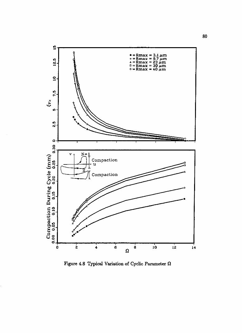
." ...
." N ...
0 ...
." r-:
u :::.
..",
."
." N
0
0 M 0
E E~ _0
C1l -00 ~'" t..>O Qi)
~ .... ." ~~ ~O
Q
~O O~
.... 0 ~ 0 ~." ~o Eo 0 0 t..>o
0 0
v
Compaction ---I-""'-+-!- U
2 6
• = Rmax = 3.1 ?Lm 0= Rmax = 9.7?Lm A = Rmax = 23 f.£m a = Rmax = 30 f.£m o = Rmax = 40 f.£m
8 10
Figure 4.S Typical Variation of Cyclic Parameter n
so
12 14

81
4.6 Specific Functions for a, exQ and r
General functions are presented for ex, aQ and r in Section 4.5. Such general
ity renders these functions applicable to any class of problems. Only disadvantage
of such general functions is that they fail to yield important and required infor
mations as demanded by any specific problem. Therefore, specialization of the
general functions is vital to suit specific problems in order to achieve required pre
dictive capability. As demonstrated later, special forms of the functions simplify
the model in terms of number of parameters and produce better predictive capa
bility. Presented in this section is the special forms of a, aQ and r derived from
general functions of ex, exQ and r.
The general function ex, Eq.( 4.26), decreases asymptotically to zero as shear
displacement becomes large. Similarly, function r Fig.( 4.7), increases from zero
to rue It could be possible either to match numerically the predicted Tp With'
experimental value or to match predicted shear displacement at which T = Tp occurs
with observed. But, both Tp and the corresponding shear displacement from model
prediction can not be matched with experimental values simultaneously owing to
the asymptotic nature of ex and r. Moreover, most of the interface test data show
occurence of Tp at very small shear displacement resembling rigid plasticity type
shear stress curve. Under these circumstances, the rate of change of a (a) is very
high, thus making the parameters a and b very sensitive to the change of interface
roughness. Instead of two parameters a and b, introducing greater number of
parameters in a can avoid the parameter sensitivity. But this would make the
model inefficient with the respect to number of parameters required to define it.
In order to circumvent parameter sensitivity and to predict Tp and corresponding
shear displacement accurately, a special form of Eq.(4.26) is presented for ex with
accompanying modification to the function r. Observe that aQ is not changed here.
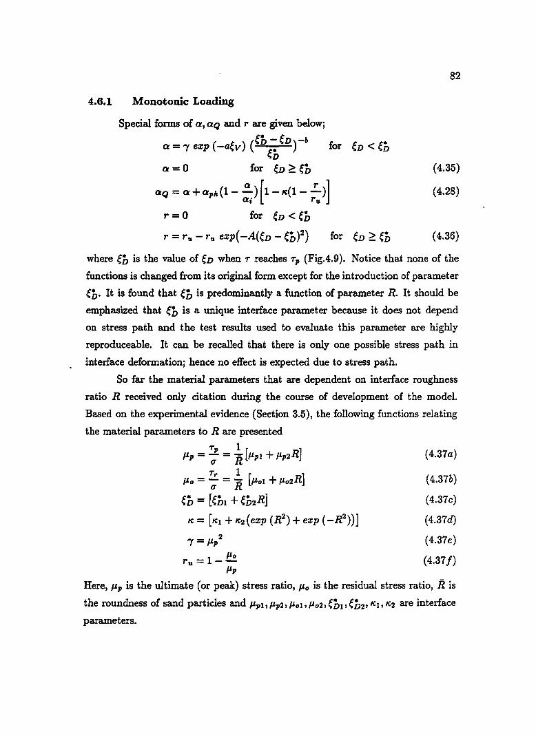
4.6.1 Monotonic Loading
Special forms of a, aq and r are given below;
a = 'Y e:cp (-aev) (eO e'b eD)-6 for eD < eD
a = 0 for eD ~ en aq = a + apia (1 - .!!.) [1 - ,,(1 - .!.)]
ai ru
r = 0 for eD < eD
r = ru - ru e:cp( -A(eD - en?)
82
(4.35)
(4.28)
(4.36)
where eo is the value of eD when T reaches Tp (FigA.9). Notice that none of the
functions is changed from its original form except for the introduction of parameter
eD. It is found that en is predominantly a function of parameter R. It should be
emphasized that en is a unique interface parameter because it does not depend
on stress path and the test results used to evaluate this parameter are highly
reproduceable. It can be recalled that there is only one possible stress path in
interface deformation; hence no effect is expected due to stress path.
So far the material parameters that are dependent on interface roughness
ratio R received only citation during the course of development of the model.
Based on the experimental evidence (Section 3.5), the following functions relating
the material parameters to R are presented
Tp 1 [ ] I'p = -; = R jJpl + I-'p2R
Tr 1 [ ] jJo = -; = R jJol + 1-'02 R
eb = [eDI + eD2R]
,,= ["I + "2 (e:cp (R2) + e:cp (_R2)]
'Y = jJp2 1-'0
ru = 1--I-'p
(4.37a)
(4.37b)
(4.37c)
(4.37d)
(4.37e)
(4.37 f)
Here, I'p is the ultimate (or peak) stress ratio, jJo is the residual stress ratio, R is the roundness of sand particles and jJpb jJp2' I-'ob 1-'02, eDI' eb2' "b ""2 are interface
parameters.

~~--~----------------~----I -- Rough Interface
It) N o
..... Smooth Interface
.,.YeD = eDCSmooth)
/ ~eD =eDCRough) o~~~~--~~~----~--~----~----~--~ -~--~----------------------I
~ N 0
0 N 0
It) ... 0
~o ... 0
It) 0 0 0 0 0
0 0.25 0.50 0.75 1
eD
1.25 1.50 1.75 2
83"
Figure 4.9 Typical Variation of (T/u),a,aQ and r at Constant Normal Stress u

84
4.6.2 Cyclic Loading
The details of general functions of a, aq and r used for cyclic loading are
elaborated in Section 4.6.1. Now, instead of general functions, special forms of a
(Eq.4.35) and r (Eq.4.36) are adopted as explained in Section 4.6.1. The special
form of aqe, Eq.( 4.33) is defined as
(4.38)
Notice that the special form of aqe is the same as that of general function aqc
(Eq.4.33), only a and r are specialized from general functions.
Based on Fig. ( 4.8), the following relation is proposed for the cyclic parameter
n· , ( 4.39)
Here nl, n2 and n3 are cyclic parameters. And Trev , and Tmax indicate the value
of shear stress at stress reversal point and maximum value of shear stress for the
cycle, respectively. The motivation behind the choice of eVe and (Trev/Tmax) in
Eq.( 4.39) is due to the discussion presented in Section 4.4.1. Inclusion of "y in
Eq.( 4.39) explicitly relates n to interface roughness ratio R.
4.1 Incremental Stress-Displacement Relation for Interface
Elasto-plasticity matrices of intact part and average response are given by
Eq.( 4. 7) and Eq.( 4.20), respectively. For the sake of completeness of the formula
tion, the elasto-plasticity matrices are elaborated in this section.
where
Employing the non-associative flow rule;
A = {> 0, =0,
for f = 0 and j > 0 for f ~ 0 and j < 0
( 4.40)
(4.41)
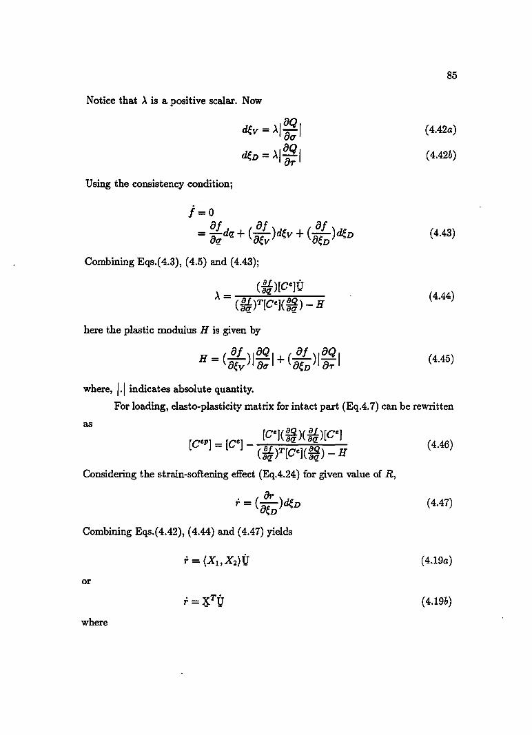
Notice that ,\ is a positive scalar. Now
Using the consistency condition;
i=o of of of
= Oqdq+ (oev)dev + (oeD)deD
Combining Eqs.( 4.3), (4.5) and (4.43);
(li. )[cenl ,\ _ aq
- (~)T[ce](~) - H
here the plastic modulus H is given by
where, 1.1 indicates absolute quantity.
85
(4.42a)
( 4.42b)
(4.43)
( 4.44)
( 4.45)
For loading, elasto-plasticity matrix for intact part (Eq.4.7) can be rewritten
as
[Cep] = [ce] _ [Ce
]( ~)( fk )[Ce]
(~)T[ce](~) - H
Considering the strain-softening effect (Eq.4.24) for given value of R,
r = ( Or )deD OeD
Combining Eqs.(4.42), (4.44) and (4.47) yields
or
where
( 4.46)
(4.47)
(4.19a)
(4.19b)

86
(4.48)
Substituting Eqs.( 4.48) and (4.46) in Eq.( 4.21), one can obtain the elasto-plasticity
matrix [Ce".] for average response of interface. Simplicity of using the special forms
of Q', r in the model can be illustrated as following for constant normal stress 0-
(1) For eD < eb;
r=O
(4.49)
r = r(eD,R)
[oep.] = - [rt~l rt~2] (4.50)
This indicates hardening takes place during eD < eb, and strain-softening takes
place after eD ~ eb. Moreover, hardening and strain softening do not occur simul
taneously and eD = eb is the point separating these two behavior. These aspects
are illustrated in Fig.( 4.9).
The elasto-plastic matrix given by Eq.( 4.20) is valid for monotonic loading.
The same relation is valid for cyclic loading as well; during cyclic loading the first
loading phase and subsequent reverse loading phases are described by Eq.( 4.20).
87
CHAPTER 5
EVALUATION OF PARAMETERS AND MODEL VERIFICATION
Calibration of a constitutive model against experimental data and verifi
cation of the proposed model are another important step in the formulation of
constitutive relationship. This chapter presents the following four different as
pects: (1) evaluation of parameters of the proposed model, (2) verification of the
proposed model, (3) physical meaning of the model parameters, and (4) analysis
of the model.
5.1 Evaluation of Model Parameters
This section is divided into two parts: First, the detail of the procedure to
evaluate parameters of the proposed model (Ch!=tpter 4) is presented. Secondly, the
calculation of model parameters using the test data presented in this chapter and
Chapter 3, is outlined. In each of the above cases, monotonic and cyclic loadings
are treated separately.
5.1.1 Procedure to Evaluate Model Parameters
5.1.1.1 Monotonic Loading
The two major classes of parameters required to define interface behavior are
elastic and plastic. The elastic behavior of interface defined by Eq.( 4.3), requires
the elastic normal stiffness /(n and elastic shear stiffness J(a. The plastic part of
interface behavior can be categorized into three components listed in hierarchical
order as (1) associative, (2) non-associative, and (3) strain-softening. Descrip
tion of associative model requires the definition of yield function f (Eq.4.11), and
evolution of hardening function a (Eq.4.35). Thus required parameters are n, "'I
and hardening function parameters eD, a and b. Non-associative model requires,

88
in addition to the definition of associative model, a plastic potential function Q, Eq.{4.14) and its evolution rule defined by O!Q, Eq.(4.28). Therefore, in this case,
non-associative parameter It is required. Finally, strain-softening behavior requires
definition of the damage evolution function r, Eq.( 4.36), thus parameters A and ru
required in this case. Thus in summarry, the required elastic and plastic material
parameters are;
(1) Elastic Parameters: K n , [(IJ
(2) Plastic Parameters:
Associative Model: n, ",(, eD, a, b
Non-Associative Model: associative model parameters and It
Strain-Softening: non-associative model parameters and A, ru
Altogether ten parameters are required to represent the strain-softening be
havior with non-associative flow rule. These ten parameters are relevent for a
given interface roughness ratio R. It has been observed from interface test data,
the parameters K 8 , ",(, a, b, eD, It and ru depend on R. Especially, the dependence of
the parameters ",(, eD, It and ru on R significantly influence the interface behavior.
Due to this reason, only these parameters are explicitly related to R in Eq.(4.37).
Further, the parameters n and A seems to be not strongly influenced by R. It is
expected that Kn would be influenced by R, however at this time, the dependence
of Kn on R is not possible to establish because of'the scarcity of experimental data.
All this time, the model parameters are assumed to be independent of rate
or frequency of loading. Procedure to evaluate material parameters is explained
below;
(1) Elastic Constants ](n and ](6:
Figure (5.1) shows normal stress vs normal displacement and shear stress vs shear
displacement curves for an interface of a given roughness. The unloading slope of
the curves shown in the figure will give values for K n and K 8'
(2) Ultimate (or Failure) Parameter "'(: Ultimate shear stress condition of interface
is given by a = 0 in yield function j, Eq.(4.11):

89
Unloading Path
~----~~------------------~~v
(a) Nonnal Stiffness
T
~~------------------------~U
(b) Shear Stiffness
Figure 5.1 Calculation of Elastic Parameters
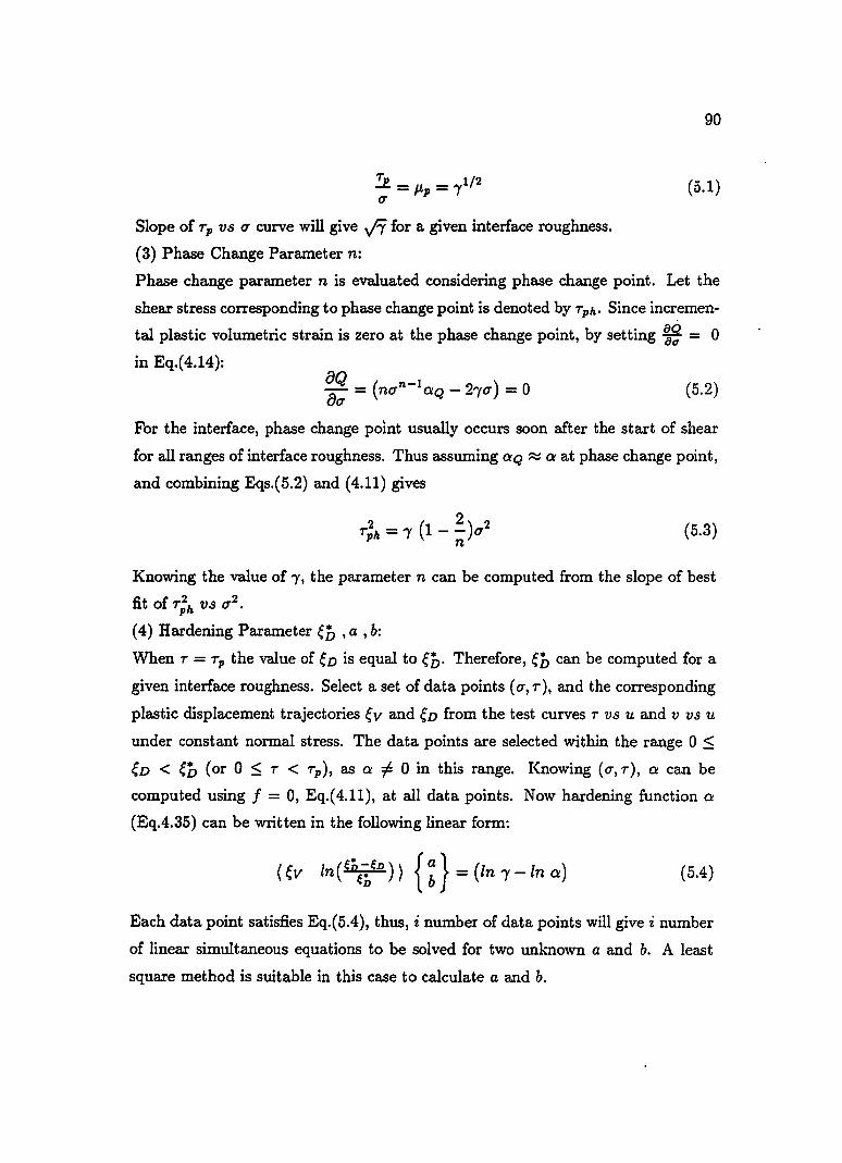
Slope of Tp vs (7 curve will give v:r for a given interface roughness.
(3) Phase Change Parameter n:
90
(5.1)
Phase change parameter n is evaluated considering phase change point. Let the
shear stress corresponding to phase change point is denoted by Tph. Since incr.emen
tal plastic volumetric strain is zero at the phase change point, by setting !f/f; = 0
in Eq.(4.14):
(5.2)
For the interface, phase change point usually occurs soon after the start of shear
for all ranges of interface roughness. Thus assuming O:Q ~ 0: at phase change point,
and combining Eqs.(5.2) and (4.11) gives
2 ( 2) 2 Tph = 'Y 1 - - (7 n
(5.3)
Knowing the value of 'Y, the parameter n can be computed from the slope of best
fit of T;h VS (72.
(4) Hardening Parameter en ,a , b:
When T = Tp the value of eD is equal to eD. Therefore, eD can be computed for a
given interface roughness. Select a set of data points (7, T), and the corresponding
plastic displacement trajectories e v and eD from the test curves T vs U and v vs u
under constant normal stress. The data points are selected within the range 0 $;
eD < en (or 0 $; r < Tp), as 0: =/: 0 in this range. Knowing (0-, T), 0: can be
computed using f = 0, Eq.( 4.11), at all data points. Now hardening function 0:
(EqA.35) can be written in the following linear form:
(5.4)
Each data point satisfies Eq.(5A), thus, i number of data points will give i number
of linear simultaneous equations to be solved for two unknown a and b. A least
square method is suitable in this case to calculate a and b.
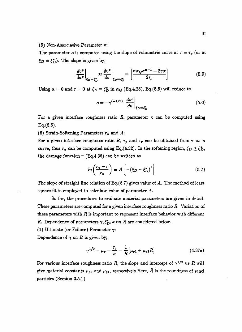
91
(5) Non-Associative Parameter ~:
The parameter ~ is computed using the slope of volumetric curve at T = Tp (or at
eD = eb). The slope is given by;
dvP I ~ dvP I = [naQO'n-l - 2'"(0'] du p ~D=ED . du ~D=~D 2Tp
(5.5)
Using a = 0 and r = 0 at eD = eD in aQ (Eq.4.28), Eq.(5.5) will reduce to
( -1/2) dvP I ~=-'"( -
du ~D=ED (5.6)
For a given interface roughness ratio R, parameter ~ can be computed using
Eq.(5.6).
(6) Strain-Softening Parameters ru and A:
For a given interface roughness ratio R, Tp and T r can be obtained from T vs U
curve, thus ru can be computed using Eq.( 4.32). In the softening region, eD 2: eD, the damage function r (Eq.4.36) can be written as
(5.7)
The slope of straight line relation of Eq.( 5. 7) gives value of A. The method of least
square fit is employed to calculate value of parameter A.
So far, the procedures to evaluate material parameters are given in detail.
These parameters are computed for a given interface roughness ratio R. Variation of
these parameters with R is important to represent interface behavior with different
R. Dependence of parameters ,"(, eD, ~ on R are considered below.
(1) Ultimate (or Failure) Parameter '"(:
Dependence of '"( on R is given by;
",,1/2 _ Il _ Tp _ 1 [Il + Il R] I - rp - - - -=- rpl rp2 0' R
(4.37e)
For various interface roughness ratio R, the slope and intercept of '"(1/2 vs R will
give material constants /-Lp2 and /-Lpl, respectively. Here, R is the roundness of sand
particles (Section 3.5.1).

92
(2) eb: Repeating Eq.(4.37c)j
(4.37c)
While R varies, the slope and intercept of eb vs R will give material constants eb2 and ebt, respectively.
(3) It:
In case of monotonic loading, repeating Eq.( 4.37d)j
By plotting It vs (e R2 + e-R2), the constants 1t1 and 1t2 can be computed.
(4) ru:
Rewriting the relationship between residual friction coefficient J.lo to Rj
Tr 1 [ ] 1'0 = -;; = R 1-'01 + l'o2 R
(4.37d)
(4.37b)
By plotting J.lo vs R, the constants 1-'01 and J.l02 can be calculated. Now ru can be
expressed as function of R using Eq.( 4.37f)j
5.1.1.2 Cyclic Loading
During cyclic loading, for small displacement amplitude (eD $ eb), the
cyclic loading parameters K n , K 8", n, a, b, eb, It, ru and A are the same as that for
the monotonic loading case. However, at large displacement amplitude (eD > eh), the required parameters" a, b, eb and It need to be reevaluated. Notice that the
strain-softening parameters ru and A are not required in this case. The same
values of Kn, 1<8 and n used in monotonic loading will be used for cyclic loading.
Moreover, cyclic loading requires determination of cyclic parameter n. The parameters to be evaluated for cyclic loading are
for (eD > eb)

93
(1) Ultimate (or Failure) Parameter ')':
Experimental observation on cyclic loading indicates that during large displacement
amplitude, the shear stress T at the ultimate state attains a value equal to Tr
observed in monotonic loading (Section 4.4.2.3). Also the value of T at ultimate
state 'in both forward and backward phases are the same. Thus, for forward and
backward phases, ')' is given by;
( 4.37b)
The procedure for evaluation of ')' is the same as that explained for monotonic
loading case.
(2) Hardening Parameters eD, a, b:
The cyclic shear stress curve T us U and u us U are used to calculate eD, a and
b. The procedure to evaluate eD, a and b are similar to that given in monotonic
loading.
(3) Non-Associative Parameter K:
Similar to monotonic loading, parameter K is computed using slope of volumetric
curve at T = Tp. It is observed that the slope of volumetric curve decreases with
number of cycles for a constant displacement amplitude test. However, such a
decrease in slope seems to be negligibly small within the first 15 cycles of loading.
Notice that the cyclic tests used herein (Section 3.4.2) are performed for maximum
of 15 cycles. Hence, it is assumed the slope of volumetric curve at T = Tp is same
for all the cycles. The procedure to calculate K is same as that for monotonic
loading. It is interesting to note that the slope of volumetric curve at T = Tp
during cycles is smaller than that of monotonic loading. Now the dependence of K
on R is expressed as
(5.8)
The parameter K is related to (e R2 + e-R2) for the monotonic loading (Eq.4.37d).
However, the Eq.(5.8) provides better correlation for K in the case of cyclic loading.
Again the procedure to evaluate KI and K2 are same as that of monotonic loading
case.

94
(4) Cyclic Parameter n: In the proposed model for cyclic loading, parameter n controls magnitude of com
paction during the reloading phase. Thus, the calculation of n is based on the
amount of compaction during reverse loadings. Since compaction is observed dur
ing each phase of reverse loading, parameter n can be calculated two times per
cycle as there are two reverse loading phases in a cycle. Similarly, n can be com
puted for all cycles. Generally compaction decreases with number of cycles and
finally reaches the steady state where no further compaction is observed. Accord
ingly, the value of n is defined such that it first decreases and then approaches
unity at steady state.
During a constant normal stress test, the shear induced volume change is essen
tially plastic; i.e dv = dvp• In order to evaluate n during compaction under reverse
loading, the incremental volumetric strain dv is integrated from the start of reverse
loading until the phase change point as shown in Fig.(5.2)j and using flow rule
(Eq.4.40), dv is written as
(5.9)
Also rewriting aqc in Eq.( 4.33),
aqc =!2a+X (5.10)
where,
X =aph(l-~) [1-11:(1- ev -tVPh)] ai eVph
(5.11)
Integration of Eq.(5.9) from the start of reverse loading upto the phase change
point (Fig.5.2), and swapping the terms leads to
(5.12)
The integration limit runs from 0 to U~h as shown in Fig.(5.2). The term v in
Eq.(5.12) indicates compaction during reverse loading. Equation (5.12) gives an
expression to evaluate n during reverse loading. This calculation can be repeated
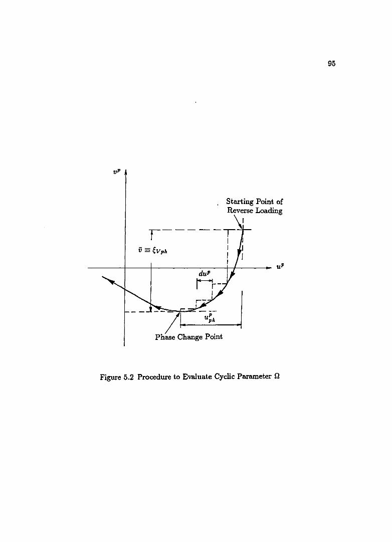
vP
Starting Point of Reverse Loading
\' r-----T I f
I f
Figure 5.2 Procedure to Evaluate Cyclic Parameter n
95

96
for all the cycles, thus, the value of n for a given number of cycles is known. The
numerical integration schemes, namely the trapezoidal or Simpson rule, can be
employed with Eq.(5.12}.
The cyclic parameter 0 is related to eVe as
( 4.39)
Here, OIt O2 and 0 3 are cyclic parameters. In the available test data, T rev = T max,
thus evaluation of parameter 0 3 is not considered at this time. Therefore, it is
assumed 0 3 = 1. Rewriting Eq.( 4.39) in linear form;
( 1 Ie) {In 0 1 } _ 1 [ 0 - 1 ] n Ve O2 - n "'I(Trev/Tmax}
(5.13)
Knowing n and eVe for all cycles, 0 1 and O2 can be computed using least square
method.
The cyclic parameter 0 or 0 1 and O2 are computed for a given interface roughness
ratio R. It is possible to relate 0 1 and O2 to R.
5.1.2 Calculation of Model Parameters
Using the procedure elaborated in Section 5.1.1, model parameters are cal
culated from the test data presented in Section 3.4.1. Presented in this section
are sample calculations of model parameters for both monotonic and cyclic load
ing, which are summarized in Table (5.1). Figure (3.5) is used with (j = 98kPa,
Dr = 90%, Rmax = 3.8,9.6, 19,40JLm (Toyoura sand-steel interface), to illus
trate sample calculations for monotonic loading. Illustration for cyclic loading
utilizes the observed curves in Figs.(5.15) and (5.17) with 0' = 98kPa, Dr = 90%,
Rmax = 23, 40 JLm (Toyoura sand-steel interface).
5.1.2.1 Monotonic Loading
Calculations for the parameters "'I, n, a, b, eD, Ii:, r" and A are given below.
( a) Ultimate (or Failure) Parameter 1:
Test data from Fig.(3.5) combined with Eqs.(4.37e) and (5.1) results in Fig.(5.3),
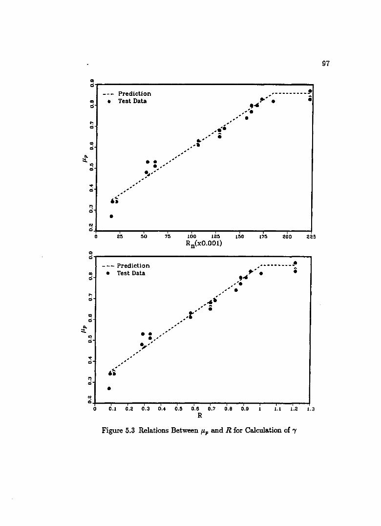
Q.
:::t
m
Q~----------------------------------------------------------~
II)
c:i
CO)
Q
N c:i
0
m c:i
II)
c:i
I': c;)
II)
c:i
It)
c:i
"" c:i
CO)
c:i
N c:i
0
• Prediction Test Data
.. ,." . " .. ~~,." , .. ' .. '
.,' ,i
• 25 50 75
- -- Prediction
• Test Data
.. , , •• .. ... " , ,-"
,
.. , , .. , , .. .. ,~
• 0.1 0.2 0.3 0.4
"
, ,
' . ... , ... , ... .... ,.". ,
100 125 Rn(xO.OO1)
,---------~ .,"" i .... . ..' . .. '
" . , ..
150
,
175 200
._------_.-,,' ... . • ,,' . ..
225
, • , , , .. -.. ... ..... .. t" .. ..
0.5 0.6 0.7 0.8 0.9 1 1.1 1.2 1.3 R
Figure 5.3 Relations Between JLp and R for Calculation of 'Y
97
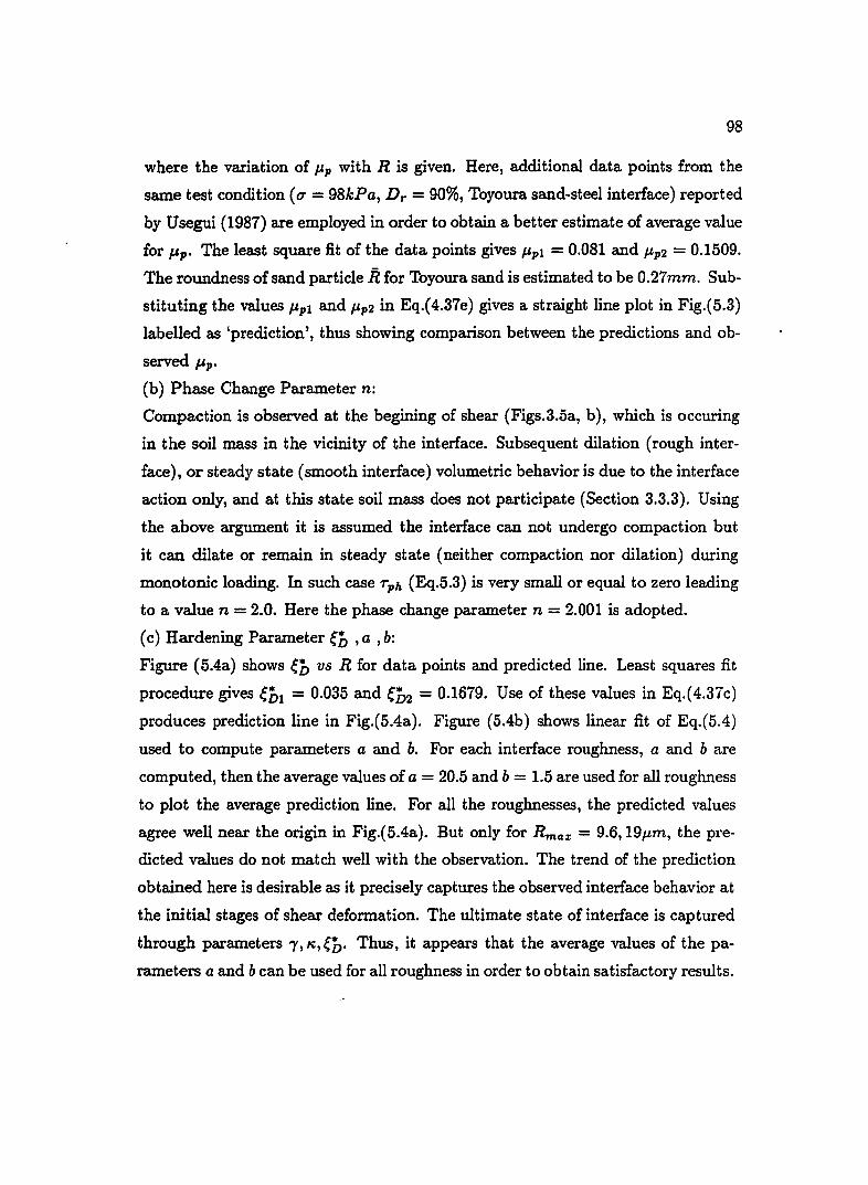
98
where the variation of J.1.P with R is given. Here, additional data points from the
same test condition (O' = 98kPa, Dr = 90%, Toyoura sand-steel interface) reported
by Usegui (1987) are employed in order to obtain a better estimate of average value
for Jl.p. The least square fit of the data points gives J.1.pl = 0.081 and J.1.p2 = 0.1509.
The roundness of sand particle R for Toyoura sand is estimated to be 0.27mm. Sub
stituting the values J.1.pl and J.1.p2 in Eq.{ 4.37e) gives a straight line plot in Fig.(5.3)
labelled as 'prediction', thus showing comparison between the predictions and ob
served Jl.p.
(b) Phase Change Parameter n:
Compaction is observed at the begining of shear (Figs.3.5a, b), which is occuring
in the soil mass in the vicinity of the interface. Subsequent dilation (rough inter
face), or steady state (smooth interface) volumetric behavior is due to the interface
action only, and at this state soil mass does not participate (Section 3.3.3). Using
the above argument it is assumed the interface can not undergo compaction but
it can dilate or remain in steady state (neither compaction nor dilation) during
monotonic loading. In such case 7'ph (Eq.5.3) is very small or equal to zero leading
to a value n = 2.0. Here the phase change parameter n = 2.001 is adopted.
( c) Hardening Parameter eD ,a ,b:
Figure (5.4a) shows eD vs R for data points and predicted line. Least squares fit
procedure gives eD1 = 0.035 and eD2 = 0.1679. Use of these values in Eq.(4.37c)
produces prediction line in Fig.(5.4a). Figure (5.4b) shows linear fit of Eq.(5.4)
used to compute parameters a and b. For each interface roughness, a and bare
computed, then the average values of a = 20.5 and b = 1.5 are used for all roughness
to plot the average prediction line. For all the roughnesses, the predicted values
agree well near the origin in Fig.(5.4a). But only for Rmax = 9.6,19J.1.m, the pre
dicted values do not match well with the observation. The trend of the prediction
obtained here is desirable as it precisely captures the observed interface behavior at
the initial stages of shear deformation. The ultimate state of interface is captured
through parameters 'Y, K., eD. Thus, it appears that the average values of the pa
rameters a and b can be used for all roughness in order to obtain satisfactory results.

I/)
~~-------------------------------------------------------------,
Q N c:i
I/) ... c:i
Prediction • Test Data
•
*1:) <.v
Q
c:i
I/) Q
c:i
g • c:i~ __ ~ __ ~ ____ ~ __ ~ __ ~ ____ ~ __ ~ __ ~ __ ~~ __ ~ __ ~ __ ~ __ ~
o 0.1 0.2 0.3 0.4 0.5 0.6 0.7
R 0.8 0.9 1.1 1.2 1.3
(a) Q,---------------------------~----------------------------~e o\\·~ .. i
... I
N I
o Rmax = 3.8 /Lm () Rmax = 9.6 IJ.m Ci Rmax = 19 /Lm c Rmax = 4-0 /Lm
··~·o·:'" " •.•••.•• ~..:,.,.:,' I
......... fIA, ..... ..-:..., ,~ . ." " ••••• t"*"fI!" ,'" ,,: I
0'" --L.;.L"'" .,.. I
......... ;lS."' ... ' " I
..... ::::::::::::::::::.~ .. ~~~~;,~,"" ,rf'" () /9 D.·::.·::····· ,,' ,,' .... "
••••••• , ", I ....... ," ..... ..~ .... ,',',00 -,' .... '" ".--
6············ "" ,g:;';"-CS..,. CI """ ,'", --
It)
I
rD I
" , , , ,,' ",
" , """ ","
,,' ,ii' A" ,
... 0'
....... Prediction --- Test Data
~~--------~,--------~--------~------~~------~--------~--------~------~ -2 -1.75 -1.50 -1.25 -1 -0.75
In[(eb - eD)/eb]
(b)
-0.50 -0.25
Figure 5.4 Calculation of Hardening Parameters
(a) Parameter eD' (b) Parameters a and b
o
99
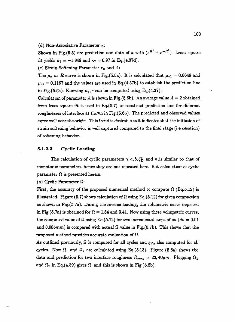
100
(d) Non-Associative Parameter It:
Shown in Fig.{5.5) are prediction and data of It with (e R2 + e-R2). Least square
fit yields Itl = -1.949 and 1t2 = 0.97 in Eq.{ 4.37d).
(e) Strain-Softening Parameter r" and A:
The 1-'0 us R curve is shown in Fig.{5.6a). It is calculated that P.ol = 0.0648 and
1-'02 = 0.1167 and the values are used in Eq.{ 4.37b) to establish the prediction line
in Fig.{5.6a). Knowing P.o, r can be computed using Eq.{ 4.37).
Calculation of parameter A is shown in Fig.{5.6b). An average value A = 2 obtained
from least square fit is used in Eq.{5.7) to construct prediction line for different
roughnesses of interface as shown in Fig.{5.6b). The predicted and observed values
agree well near the origin. This trend is desirable as it indicates that the initiation of
strain softening behavior is well captured compared to the final stage (i.e cesation)
of softening behavior.
5.1.2.2 Cyclic Loading
The calculation of cyclic parameters "),, a, b, eiJ and It .is similar to that of
monotonic parameters, hence they are not repeated here. But calculation of cyclic
parameter n is presented herein.
(a) Cyclic Parameter n:
First, the accuracy of the proposed numerical method to compute n (Eq.5.12) is
illustrated. Figure (5.7) shows calculation ofn using Eq.{5.12) for given compaction
as shown in Fig.{5.7a). During the reverse loading, the volumetric curve depicted
in Fig.(5.7a) is obtained for n = 1.84 and 3.41. Now using these volUI]letric curves,
the computed value of n using Eq.{5.12) for two incremental steps of du (du = 0.01
and 0.005mm) is compared with actual n value in Fig.(5.7b). This shows that the
proposed method provides accurate evaluation of f2.
As outlined previously, n is computed for all cycles and eVe also computed for all
cycles. Now f2l and f22 are calculated using Eq.{5.13). Figure (5.8a) shows the
data and prediction for two interface roughness Rmaz = 23,40p.m. Plugging f2l
and f22 in Eq.(4.39) gives n, and this is shown in Fig.{5.8b).

10
~~------------------------------------------------------~ o o ..;
o I(~
o
10 N ci
--- Prediction • Test Data
o __ ----~ .---------- .. ---10 N
, , , , , __ -------4'
, " .
" , , , ,
,,' " ~",
, ,
, "",
". "
~~----~----~----~----~------~----~----~----~----~ 0.1 0.2 0.3 0.4 0.5 0.6 0.7 0.8 0.9
Figure 5.5 Calculation of Non-Associative Parameter It
101

;;-$.. ........ -. $..
I =
$.. --1: -
loo 0,-------------------------------------------------------,
C')
0
N 0
0
C 0
I/')
0 I
C! -I ~ ... I
C iii I
It)
iii I
- -- Prediction • Test Data
'" .... •
,. . •
•• • ••
0.1 0.2 0.3 0.4 0.5 0.6 0.7 0.8 0.9
(a)
• •
1.1 1.2 1.3
g4 ¢ Rmax = 3.8 /Lm 6 Rmax = 9,6 /Lm ~ Rmax = 19 p,m o Rmax = 40 p,m
g'O" ... .er.,'~, ~E"""D"' .0-
0
0- - - - CIr..... - o' .. ..0 - - - - .~. - - -~O' ~ ·0' -_____ .Q::: :_A ----'B_.,~.fr:. 0- -"
_ - - [J __ -A <> __ '" . ...0--- fl--- . J.J • .. .. " ";./j. .. " .. " .. .. ": .... ",, .0'" '?:---- .<0" G'" ~ --.~'" ,."
.¢ ... -,' ,0 ....... .,0' .
__ .0"- ,- .... cr 0- - - - -.-",0' ,.0
,.... .[3",.,
..0-,- 0····· .... " "
c M I 0--- •.•.. Prediction
- - - Test Data It)
M I
C .; o· I~~--~------~----~,------~----~------~----~----~ -2 -1.75 -1.50 -1.25 -1 -0.75 -0.50 -0.25
-(eD - eb) (h)
Figure 5.6 Calculation of Strain-Softening Parameters
(a) Parameter T", (b) Parameter A
o
102

S E ->
ci,~~----------------------------------------------~ "
I/) 0 ci I
0
ci I
I/) ...
,-,-, ' , ' , "-, , - .. , " .. . .. - ". - .. - ' ..
" ,.. .... fill tit ...
" ..... -.. .. .. \ ---. " --.
" .. ... .... ... .... .. n 1 84 ___ u = . " --.-.- .. _-------------'. ........
...... ....... .... .... .... ...... ...... .... - ... --- ...... ----------------{2 = 3.41
~f_------~--------~--------~------~--------~------_J 0.0 0.1 0.2 0.3 0.4 o.~ 0.6
(a)
.~----------------------~----------------------
- - - Exact Value -. ·0·- Small du Step -·.·-Large du Step
n = 1.84 N ...--·_-_·_-·---·4-·--·--_· __ · .. __ ·_··
;.t..~~.~ __ <>www~wwwOwwwwOwwwwowwwwowww~owww~www~www~w __ ~
:3 a
0.0 0.1 0.2 0.3 0.4 o.~ 0.6 eD
(b)
103
Figure 5.7 Accuracy of Numerical Method to Compute Parameter n: (a) Volumetric Com-
paction During Reloading, (b) Calculated n for Various Step Sizes of du

1= --.... I
c: ;::: .s
c:
Q ...
CD Q
co Q
...... Prediction - --Test Data
(II
Q~------~----~------~------~----~~----~------~----~ -2 -1.1i -1 -O.1i o In(eve)
O.S 2
Q (a) ~,---------------------------~~--------------------------~
CD N
(II
N
CI , , , , , , , , , Q ,
'. , '. ,
..... " "0. ,
'. , '., .. ,'. Q ':''0.
" " t ••••••
Q,~,\ ,0." o '. 'c ........... ··c ..... P", "0 '0 .. 0 .. 0"'0.. ...... ···0 ....
...... Prediction - - - Test Data
o Rmax = 23 tJ.m o Rmax = 40 tJ.m
"0'* .. '(). •. ,Q" 0---0 0 .. "0* ~g·:'·8"~·"8'.:"8'.~.8~X) ~o-~·.Q·~·~o,,_ . .o. --0-- 0-_
Q ~"o.:-a [J'!Jo· ... o.... -0--0-_ N~ ____ ~ ____ ~ ____ ~ ____ ~ ____ ~ ____ ~ ____ ~ ____ ~·_o_ .. _·._.o~·_ .. _.o_._ .. ~,
o O.1i 1.1i 2 2.1i
eVe (b)
3 3.1i .. ~ 5
104
Figure 5.8 Calculation of Cyclic Parameters 0 1 and O2 (a) Linear Fit for 0 1 and O2 , (b) .
Comparison of 0 with Test Data and Prediction
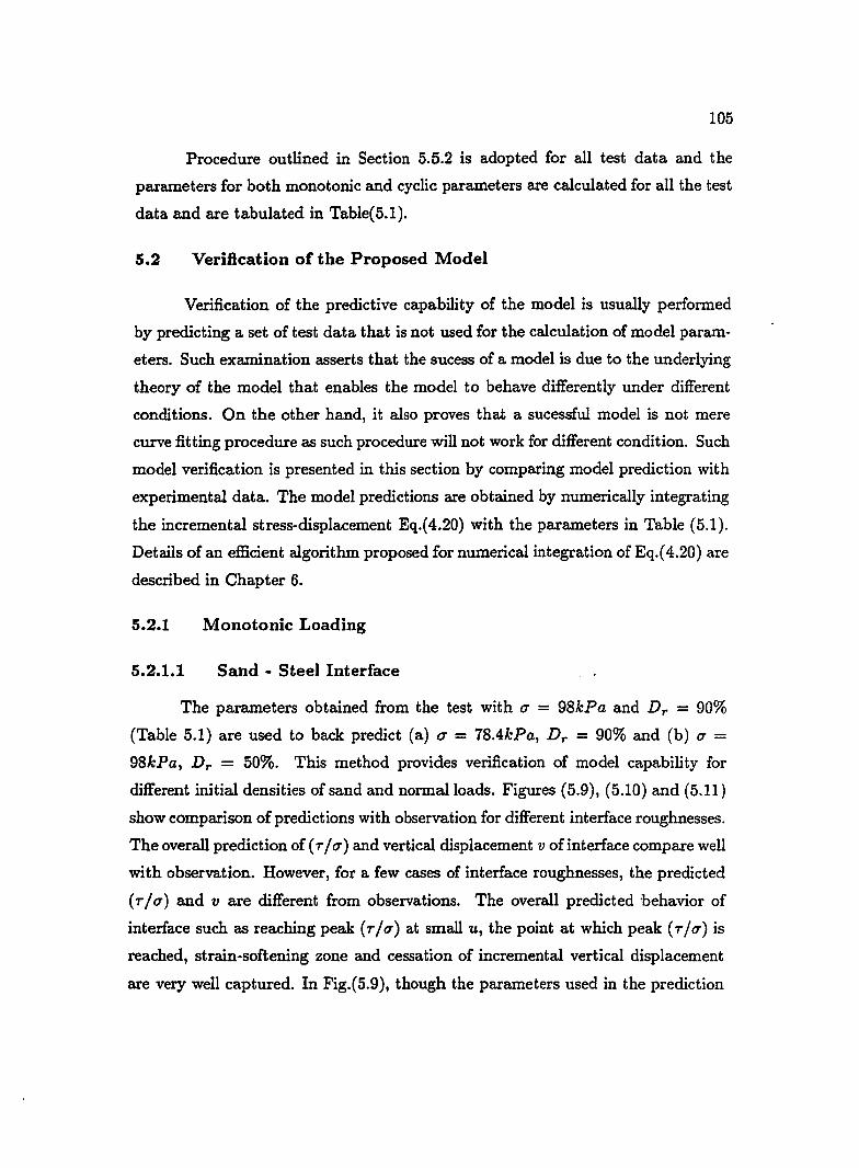
105
Procedure outlined in Section 5.5.2 is adopted for all test data and the
parameters for both monotonic and cyclic parameters are calculated for all the test
data and are tabulated in Table(5.1).
5.2 Verification of the Proposed Model
Verification of the predictive capability of the model is usually performed
by predicting a set of test data that is not used for the calculation of model param
eters. Such examination asserts that the sucess of a model is due to the underlying
theory of the model that enables the model to behave differently under different
conditions. On the other hand, it also proves that a sucessful model is not mere
curve fitting procedure as such procedure will not work for different condition. Such
model verification is presented in this section by comparing model prediction with
experimental data. The model predictions are obtained by numerically integrating
the incremental stress-displacement Eq.(4.20) with the parameters in Table (5.1).
Details of an efficient algorithm proposed for numerical integration of Eq.( 4.20) are
described in Chapter 6.
5.2.1 Monotonic Loading
5.2.1.1 Sand - Steel Interface
The parameters obtained from the test with q = 98kPa and Dr = 90%
(Table 5.1) are used to back predict (a) (j = 78.4kPa, Dr = 90% and (b) q =
98kPa, Dr = 50%. This method provides verification of model capability for
different initial densities of sand and normal loads. Figures (5.9), (5.10) and (5.11)
show comparison of predictions with observation for different interface roughnesses.
The overall prediction of ( T / q) and vertical displacement v of interface compare well
with observation. However, for a few cases of interface roughnesses, the predicted
( T / q) and v are different from observations. The overall predicted behavior of
interface such as reaching peak (T / q) at small u, the point at which peak (T / q) is
reached, strain-softening zone and cessation of incremental vertical displacement
are very well captured. In Fig.(5.9), though the parameters used in the prediction
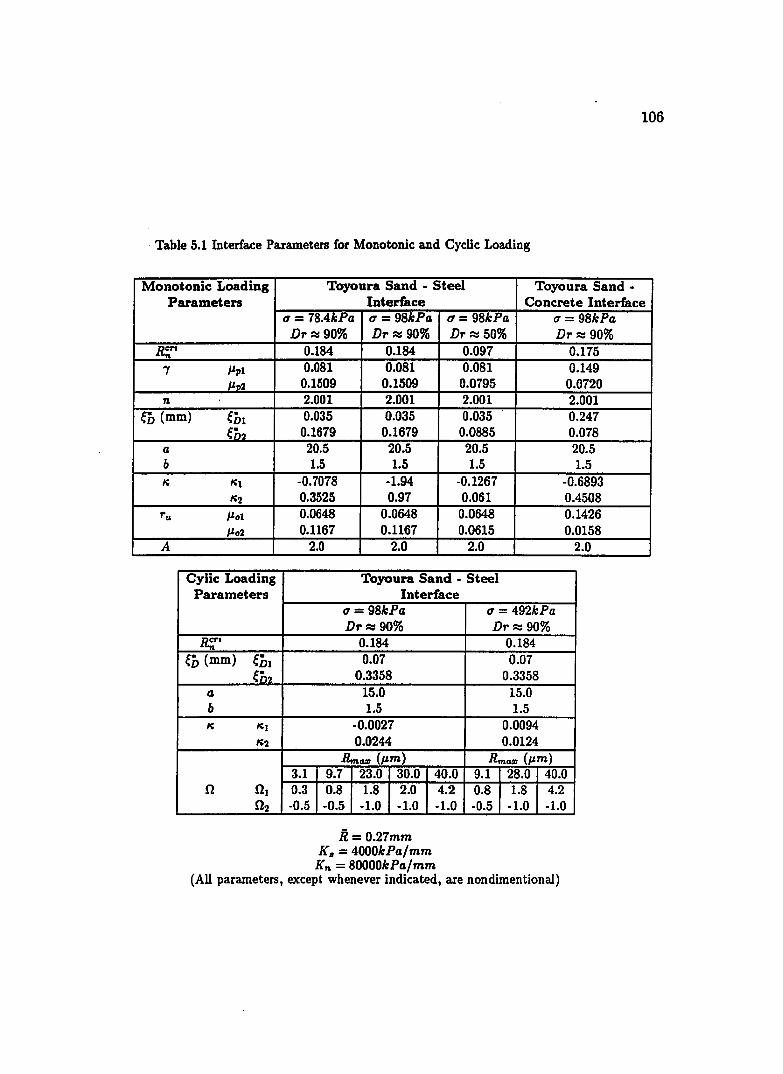
106
. Table 5.1 Interface Parameters for Monotonic and Cyclic Loading
Monotonic Loading Toyoura Sand - Steel Toyoura Sand -Parameters Interface Concrete Interface
RCT1 n
"'( IIpl
IID'l
n eD (mm) eDI
en2 a b ~ ~1
~2
ru 1101 1102
A
Cylic Loading Parameters
~' eb (mm) eDl
en2 a b ~ ~1
~2
n nl
n2
a = 78.4kPa a = 98kPa a= 98kPa a = 98kPa Dr =:: 90% Dr =:: 90% Dr =:: 50% Dr =:: 90%
0.184 0.184 0.097 0.175 0.081 0.081 0.081 0.149 0.1509 0.1509 0.0795 0.0720 2.001 2.001 2.001 2.001 0.035 0.035 0.035 0.247 0.1679 0.1679 0.0885 0.078 20.5 20.5 20.5 20.5 1.5 1.5 1.5 1.5
-0.7078 -1.94 ·0.1267 -0.6893 0.3525 0.97 0.061 0.4508 0.0648 0.0648 0.0648 0.1426 0.1167 0.1167 0.0615 0.0158
2.0 2.0 2.0 2.0
Toyoura Sand - Steel Interface
a - 98kPa a = 492kPa
3.1 0.3 -0.5
Dr::=: 90% 0.184 0.07
0.3358 15.0 1.5
-0.0027 0.0244
Rmaz (11m ) 9.7 23.0 30.0 40.0 0.8 1.8 2.0 4.2 -0.5 -1.0 -1.0 -1.0
R= 0.27mm K. = 4000kPa/mm Kn = 80000kPa/mm
Dr =:: 90% 0.184 0.07
0.3358 15.0 1.5
0.0094 0.0124
Rmaz (11m ) 9.1 28.0 40.0 0.8 1.8 4.2 -0.5 -1.0 -1.0
(All parameters, except whenever indicated, are nondimentional)

>
...
It) N c::i
o
It)
Predicted Observed
~ ... - -<>- Rmax=3.8 J,£m ....... -ll- Rmax=9.6 J,£m _.- -0- Rmax=19 J,£m -.- -0- Rmax=40 J,£m
Rmax = 40 J,£m
to'-~ = 19 J,£m 'll . ..........,;;._._._._. ...... -ll-ll
'. II ~ ....... = 9.6 J,£m .. ............................................................................ t. .... ...................... '0 ............. ~ = 3 8'p'm
'-o ..... o~¢-----------·-o-----·--··-·----- -t·-·~- .... _.-
c::i,-----------------------------------------------------~
___ )~ _Rmax = 40 :m __ -t
M c::i
... c::i
._. __ . __ . __ . __ . __ . __ .L.19 J,£~ __ •
o c::i _wwww ............ • .... · .. ww tt u4.:==~;~::--~cccw
~I.l ..... l:l-Il. ,= 3.8 I'm
0---0--0-0 o------------------~------------.
~4-------~------~------~----~------~------~------~ 0.0 1.0 2.0 3.0 4.0 5.0 6.0 7.0
U (mm)
Figure 5.9 Comparison of Model Prediction with Obsen-ation: (1 = 98kPa,
Dr = 90%, Steel-Toyoura Sand Interface. Monotonic Loading
107

>
.n C\J ci
o
.n
Predicted Observed - --- -ll- Rmax=6.8 pm , •• ".0 -0- Rmax=9.8 pm -,- -0- Rmax=22 pm
f .L\.
"'-.. '-..._._. Rmax = 22 pm
fA",,· .... ,= 9.8 u.m r-- .. - "':'"' - - ,f.
... ' ....... :·: •••••••••••••••••••••••••••••••••••••••••••• 11 ••••••••••••••••••••••••••••••••••••••••• 11 ••••••••••
------------------------.-----------_._---_._._--~ll-ll-ll-ll II ~t 6.8 pm
ci~----------------------------------------------------~
C') ci
.--,--,--.--.--.j~~~.~. ... ci
o ¥= 9.8 pm o __ • __ .wwww_w~_www_ww_ww_.www __ w_w _____ w ____ w _____ w_w __ w_
ll-t. II 1t,\ = 6.8 pm .... ci I
0.0 1.0 2.0 3.0 4-.0 5.0 6.0 7.0 u(mm)
Figure 5.10 Comparison of Model Prediction with Observation: q = 78.4kPa,
Dr = 90%, Steel-Toyoura Sand Interface. Monotonic Loading
108

>
It) N c:i
Predicted Observed -0- Rmax=9.2 I'm -0- Rmax=21 p.m
J'\. .....
II: .................. ~----------O----r-------J f····,,·... It. Rmax = 21 p.m ~ ................................................................ ./f. .................................. . ;,. .... :-...,
-. ..L •• _- --.- -- -- --- --------- ---- --- ---~~ 9~ij.,.-~- -- --
o~------~------~------~------~------.-------~----~ It)
c:i~----------------------------------------------------~
M c:i
... c:i iamax -21 ,.m ~ .. ::::'~'~'~'~'~'~'~'~'~'~ .~.~.~.~.~.~.~.~.~.~.~.~.~.~.~.~.~.~.~.~.~.~ .~.~.~.~.~ .~.~.~ '~'1~~ ·~·~i·i.;;~·~·~·~ .~ ... ~~------~------~------~------~------~------~----~
0.0 1.0 2.0 3.0 4.0 5.0 6.0 7.0 u(mm)
Figure 5.11 Comparison of Model Prediction with Observation: q = 98kPa,
Dr = 50%, Steel-Toyoura Sand Interface. Monotonic Loading
109

110
are computed from the same test presented in this figure, prediction does not
exactly match with observation. This is due to the fact that the functions relating
the parameters "),, eD' K, r, and interface roughness ratio R, are chosen in order to
satisfy the whole range of R; implying that these functions are not necessarly exact
for the whole range of R. Also the parameters a, h, and A are average parameters
for all the roughnesses. These are true in the case of (a) 0' = 78.4kPa, Dr = 90%
and (b) 0' = 98kPa, Dr = 50%.
It is observed here that the model does not predict compaction at small in
terface roughnesses. This is due to the fact that the compaction at the begining of
shear deformation of interface during monotonic lo~ding is due to the soil mass, and
at this stage interface does not show normal deformation. And the measured verti
cal displacement includes the compaction of sand mass, and this compaction is not
removed from the observed data in Figs.(5.9) to (5.11). As seen from these figures,
the predicted vertical displacement is almost zero for small interface roughness.
5.2.1.2 Sand - Concrete Interface
Figure (5.12) shows comparison of prediction with observation for three
different roughnesses. The parameters for sand-concrete interface presented in
Table (5.1) are calculated from the test data presented in Fig.(5.12), and the same
parameters are used for back prediction. Except the volumetric behavior for the
roughness Rmaz: = 19jLm, predicted and observed behavior of interfaces compare
well.
5.2.2 Cyclic Loading
Figures (5.13) to (5.20) show comparison for cyclic loadings for tests with
(a) 0' = 98kPa, Dr = 90% and (b) 0' = 492kPa, Dr = 90% for various steel-sand
interface roughnesses. These test data represent large displacement amplitude with
frequency O.OlH z. For the first phase of the first cycle, the monotonic parameters
in Table (5.1) (0' = 98kPa, Dr = 90%, steel-sand) are used. The predicted stress
ratio (T / 0') curves compare well with experimental curves. For rough interfaces,
different (T /0') curves are obtained at different cycles during the hardening phase.
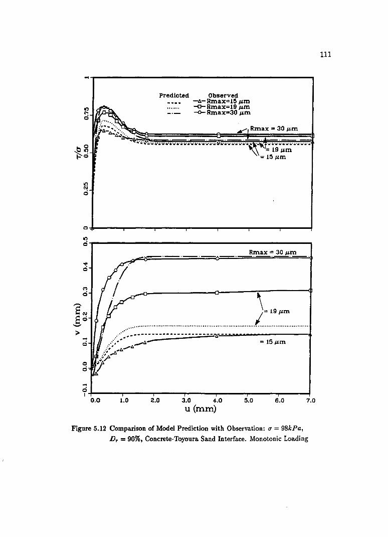
Predicted Observed -/j.- Rmax=15 p.m -0- Rmax=19 p.m -0- Rmax=30 p.m
0
It)
0 _. __ . __ . ____ . __ R~,,:, 30 p.~.
~
0
M 0
-SN So -> ... 0
0 0
\ ;= 19 p.m
, ............................................................................................... . ............ _ ••• - _ •• _. _. - - - - - - _. '"A.~-:.:-..a.-~--------+ .... > ..... ~A- = 15 p.m
.:,' A.."A ." ..Il' :~
7 ... ~~------~------~------~------~----~~----~------~ 0.0 1.0 2.0 3.0 4.0 5.0 6.0 7.0
u(mm)
Figure 5.12 Comparison of Model Prediction with Observation: (f = 98kPa,
Dr = 90%, Concrete-Toyoura Sand Interface. Monotonic Loading
111
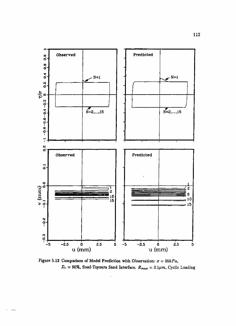
<= c::i
rc c::i .p c::i
N c::i
N c::i I
.p c::i I
rc c:i I
co c:i I
... I
N c:i
.. c::i
N c::i I
CO)
c::i I -5
Observed
~N=l
.~ N=2, ... ,15
Observed
-2.5 0 2.5 u(mm)
112
Predicted
~N=l I
N~2, ... ,15
I
Predicted
~1 =="'=====~ 2 2 10 15
6 ________ -+========~10
---------+---======15
5 -5 -2.5 0 2.5 5 U (mm)
Figure 5.13 Comparison of Model Prediction with Observation: (j = 98kPa,
Dr = 90%, Steel-Toyoura Sand Interface. Rma:c = 3.1Jlm, Cyclic Loading
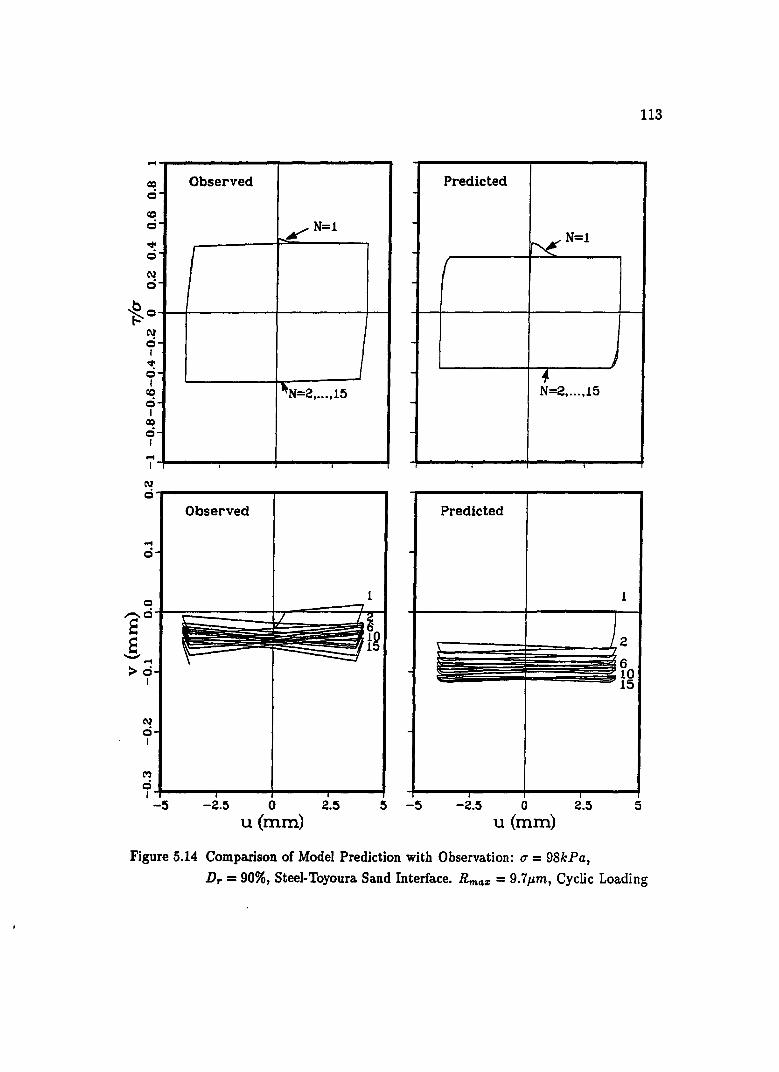
= c:i (Q
c:i ~
c:i N c:i
N c:i I ~
c:i I
(Q
c:i I = c:i I ... I
N
Observed
/N=l
I
J ~N=Z •...• 15 -
ci~----------~~----------~
... ci
N c:i I
Observed
M
~~----~----~-----T----~
-
-5 -2.5 0 2.5 5-5 u(mm)
Predicted
~N=l
f
~ N=Z •... ,15
Predicted
-2.5 0 2.5
u(mm)
Figure 5.14 Comparison of Model Prediction with Observation: q = 98kPa,
113
J
1
5
Dr = 90%, Steel-Toyoura Sand Interface. Rma:z: = 9.7J.Lm, Cyclic Loading
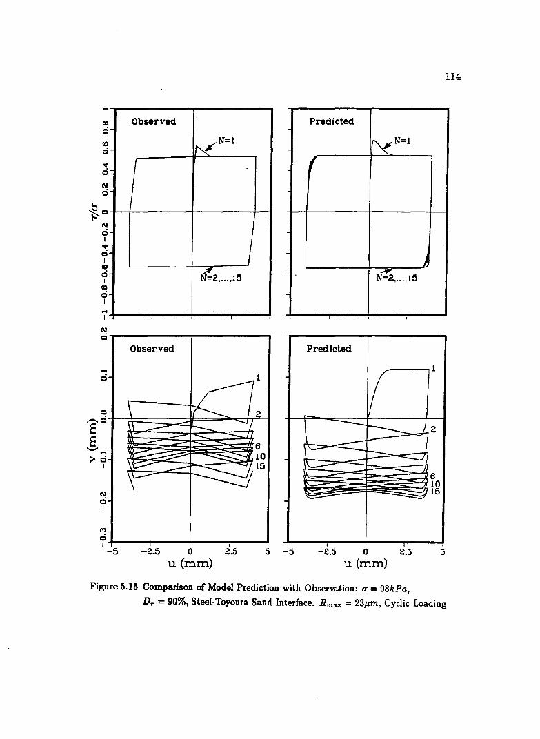
... CI)
o rc o ~ o N o
N o I ~ o I
CO o I
CI)
o I ... I
N
Observed
~ N=l
f
-
N!Z •...• 15
o~------------~-----------,
N o I
Observed
M
~~----~------~----~I----~
-
-5 -2.5 0 2.5 5-5
u(mm)
Predicted
It-tN=l
r
1. -:r
N=Z •...• 15
I I
Predicted
If 1
--r--- .1 Z ---~ '-- -- ~
~ 6
~ 10 15
~ ---=
I
-2.5 0 2.5 u(mm)
Figure 5.15 Comparison of Model Prediction with Observation: q = 98kPa,
114
I
5
Dr = 90%, Steel-Toyoura Sand Interface. Rma:c = 23j.lm, Cyclic Loading

...
N c:i I ~
c:i I
co c:i I
(I)
c:i I
... I
N
Observed
~
-
-~ N=2,.u,15
I
o'-----------~~-----------,
N c:i I
Observed
~~~~~~~~~~:o 15
M
~~----~----~~----~----~ -5 -2.5 0 2.5 5-5
u(mm)
Predicted (\(N=1
(
1 .'! N=2, ... ,15
Predicted ._---.1
-2~ 0 2~
u(mm)
Figure 5.16 Comparison of Model Prediction with Observation: (1 = 98kPa,
115
I
5
Dr = 90%, Steel-Toyoura Sand Interface. Rmaz = 30J,Lm, Cyclic Loading

= Q
rc Q
• Q
tv Q
tv Q I
• Q I
rc Q I
= Q I
... I
•
Observed
~
- j , N=2, ... ,15
I
Q~----------~-----------1~ -----,
N Q
Observed
., ~~----~----~------~----~
-
-5 -2.5 0 2.5 5-5 u(mm)
Predicted (\(N=1 ,
J. '!'-N-2, ... ,15
I
Predicted __ ---,1
6
-2.5 0 2.5 u(mm)
Figure 5.17 Comparison of Model Prediction with Observation: (1 = 98kPa,
116
5
Dr = 90%, Steel-Toyoura Sand Interface. Rmaz = 40jtm, Cyclic Loading

...
N c:i 1 ~ o
1 CD C 1 = c:i 1
.... 1
Observed
I
N=1 /
I ..... ,
1 l N=2, •.. ,15
I
~,-----------~~----------~
.... c:i
N c:i
1
~
Observed
~7~±S~~-;Jj; 6
~~--~~~ __ ~10
15
o~ ____ ~ ____ ~ ______ ~ ____ ~ 1 -5 -2.5 0 2.5 5-5
u(mm)
Predicted
I~N=1
/
I N=2, ... ,15
I
Predicted
\
, -2.5 0 2.5
u(mm)
Figure 5.18 Comparison of Model Prediction with Observation: (f = 492kPa,
117
j
1
)2 I
6 10 15
5
Dr = 90%, Steel-Toyoura Sand Interface. Rma:z: = 9.1JLm, Cyclic Loading

...
~ C I ~
ci I
"! c I
co ci I
... I
Observed - N=1
t-L--
-
- 1 N=2, •.. ,15
ci,-----------~~----------~ Observed
... o 1
c ~o~-------------------------~---------------~-----~
S - ... >0 I
N o I
n--_--=-l::::--,2
~~~6 ~~~~~~~~10
15
C')
~~--~~----~,------~----~ -5 -2.5 0 2.5 5-5
u(mm)
Predicted
(\(N=1
(
1 K
N=2, ... ,15
I I
Predicted
___ """"Tl
2
-2.5 0 2.5 u(mm)
Figure 5.19 Comparison of Model Prediction with Observation: (1 = 492kPa,
118
5
Dr = 90%, Steel-Toyoura Sand Interface. RmGII: = 28jLm, Cyclic Loading

... IX) Observed 0 rD 0 .. 0 N 0
~o ~
N 0 I .. 0 I
CQ 0 , I IX)
0 N=2 •...• 15 I ... I .. 0
Observed 1
N 0
-So 2 So -> 6 10
N 15 0 I
.. ~~----~----~------~----~
-
-5 -2.5 0 2.5 5-5
u(mm)
Predicted (\(N=1 ,
j .~ N-2 •...• 15
Predicted __ --.1
6
-2.5 0 2.5 u(mm)
Figure 5.20 Comparison of Model Prediction with Observation: (T = 492kPa,
119
,
5
Dr = 90%, Steel-Toyoura Sand Interface. Rmaz = 401lm, Cyclic Loading

120
Subsequently all the curves reach the same peak value. At small number of cycles,
vertical displacement (or ev) is higher than at larger number of cycles, thus the
hardening parameter Ct (Eq.4.35) reaches zero faster at small number of cycles.
Therefore, (7'/ u) curve at small number of cycles reaches its peak value quicker
than for large number of cycles and this leads to different (1'/ u) curves during the
hardening phase of cyclic loading. The predicted vertical displacement indicates
the trend of compaction during cyclic loading. Also, notice that the compaction
takes place during the reloading phase. With increasing number of loading cycles
eVe increases and resulting in smaller n (Eq.4.39), thus the magnitude of com
paction reduces as the cyclic loading progresses. During the initial phase of the
first cycle, vertical displacement compares well with observation for rough inter
faces, however in the subsequent cycles, the observed behavior does not match
closely with experimental values. Nevertheless the overall vertical displacement
behavior is considered satisfactory. Evidently, the final compactions calculated at
the end of 15th cycle increases with the increase in the roughness of the interface.
Comparisons of predicted and observed behavior for u = 492kPa, Dr = 90%
are shown in Figs.(5.18), (5.19) and (5.20) for three different roughness. The cyclic
parameters presented in Table (5.1) for u = 98kPa, Dr = 90% are used in the
back prediction. Observe that the cyclic 11:1 and 11:2 are different for u = 98kPa and
u = 492kPa. Still the predicted vertical displacement behavior compares well with
observed behavior. Note that (Figs. 5.17 and 5.20) for given interface roughness,
larger normal stress produces larger net compaction though the numerical difference
is small. This predicted behavior is similar as in the case of soil mass behavior. This
indicates that the model prediction of (1'/U) is same regardless of the magnitude
of u, but the volumetric prediction is affected by the magnitude of u.
The observed volumetric behavior shows that the magnitude of compaction
during the first cyclic reloading phase is very large compared to the subsequent
reloading phases where the magnitude of compaction virtually remains the same,
and resulting in net compaction as the number of cycle increases. Mathematica.lly
it is difficult to model above mentioned peculiarity of volumetric behavior, as the
smooth and continuous functions used in the model (such as Ct,CtQ,r etc.) would

121
not permit such behavior. However, the model prediction shows larger compaction
during reloading phase of first cycle followed by gradually decreasing volumetric
compaction with increasing number of cycles. At small interface roughnesses, for
example Figs.(5.l4) and (5.18), the predicted volumetric compaction at the end of
15th cycle for (7 = 492kPa is greater than that for the case (7 = 98kPa, though
the same parameters are used for the prediction of both cases. However, compari
son of predicted and observed volumetric behavior is satisfactory for (7 = 492kPa
(Fig.5.l8), whereas for the case of (7 = 98kPa (Fig.5.l4) comparison is not satis
factory. This is because, at small values of (7, the eVe at the end of first phase of
first cycle is small and this makes the computed cyclic parameter n from Eq.(4.39)
sensitive, whereas for larger (7 such sensitivity does not affect the prediction.
5.2.3 Comments
Predicted stress ratio (T/(7) vs u compares well with the observed behaviour
for both monotonic and cyclic loadings. . Predicted volumetric behavior is sat
isfactory as it reveals the general trend of observations and compares well with
numerical magnitudes of the observed volumetric values. Since the test data for
the cyclic loading represents large displacement amplitudes, the calculated param
eter n (or n1 and n2) is valid for large displacement amplitude. If test data on
small displacement amplitude also become available, it is possible to examine the
effect on n of both small and large amplitude. The cyclic parameter", (or "'1 and
"'2) is assumed to be constant throughout the cycles based on the observation of
available test data for 15 cycles. Ideally, making "', i.e slope of (~:=), decrease
with large number of cycles would produce cessation of dilation at large number of
cycles. Under this condition, while", decreases with the number of cycles, n also
decreases and approaches unity, thus a steady state is reached where no change
in the magnitude of volume occurs. In summary, the proposed method to model
cyclic volumetric behavior is general, and valid for small and large displacement
amplitudes. Availability of test data for large number of cyclic loading and small
displacement amplitude would enable one to generate improved parametric value
122
for n and K. (cyclic), so that cyclic volumetric behavior can be predicted with
improved accuracy.
5.3 Physical Meaning and Sensitivity of Model Parameters
Proper interpretation of experimental data is an essential input for constitu
tive model parameter calibration. This implies that the model parameters should
have specific physical meanings thereby the parameters can be uniquely related
in one to more states of mechanical response of material or test data. Hence, a
successful constitutive model should have parameters with physical meaning. N a
ture of constitutive model pr~diction depends on the input material parameters
meaning that the model prediction could be sensitive to model parameters. Identi
fying material parameters that are sensitive to model prediction is vital aspect as a
model user can pay special attention while computing those parameters appropri
ately, and also to foresee the effect of model prediction due to the variation in these
parameters. Firstly, in this section the physical meaning of material parameters are
identified. Then a brief account on the sensitivity of the parameters is presented.
(a) The Interface Roughness Ratio R:
The parameter R defines relative roughness of interface. It has been demonstrated
before that R strongly influences the stress-strain behavior of interface. The pa
rameter R plays a similar role to that of relative density Dr in the soil mass. The
similar behavior of loose sand and smooth interface, and dense sand and rough
interface would explain the identical role played by Dr and R in soil mass and
interface behavior, respectively.
(b) Ultimate (or Failure) Parameter "(:
The parameter "( defines the ultimate stress state of interface in a manner similar to
that of Coulomb friction angle l/J in soil mass. At ultimate state, without cohesion,
one can establish that fi is similar to tan l/J.
( c) Phase Change Parameter n:
The phase change parameter n defines the phase change point. Other terminol
ogy identifying the same phenomenon is phase transformation point (Ishihara &

123
Towhata, 1982). Introducing the parameter n permits transition of volumetric
behavior from compaction to dilation. Volumetric transition is decided by phase
change line (Fig.4.2) whose orientation is entirely controlled by the magnitude of
the parameter n. This fact can be clearly visualized in the case of associative How
rule where a stress point below or above phase change line will produce compaction
or dilation, respectively during plastic deformation. Proper control of parameter
n would allow modeling of compacting materials and also material showing com
paction and dilation.
(d) The Parameter eD: The parameter eD defines the prepeak (or hardening phase) and post peak (or soft
ening phase) on interface (Chen & Schreyer, 1987).
(e) Non-Associative Parameter 1\::
The parameter I\: is related to the slope of vertical displacement at peak stress of
interface. In other words, incremental ratio (plastic) of vertical displacement to
shear displacement (g::) is defined by the parameter 1\:. In the postulate, the pa
rameter II: is related to interface roughness ratio R. It should be recalled that aQ
(or potential function) in the proposed interface model is postulated on the basis
of dilatancy factor, (g::). (f) Cyclic Parameter n: The parameter n represents the effect of reloading, cyclic densification and par
ticle reorientation thus volumetric anisotropic effect during cyclic loading of the
interface etc.
Statistical methods render proper analysis of sensitivity of model parame
ters. Application of statistical methods is out of scope of this study. However, the
predicted behavior is found to be sensitive for the parameters j1.P' j1.o, I\: and n.
5.4 Analyses of the Proposed Model
Brief analysis of volumetric behavior and strain-softening behavior are pre
sented in this section. Further, the model behavior for constant volume condition
during monotonic loading and the effect of small displacement amplitudes during
cyclic loading are discussed herein.
124
5.4.1 Volumetric Behavior
From Eq.( 4.40) the incremental plastic normal displacement is written as
(5.14)
The plastic parameter A is positive. Thus the sign of vP depends on the sign of
(~ ) j and (~) can be positive, zero or negative implying that the incremental
plastic volume (or displacement) involves compression, no volume change or dila
tion, respectively. For a general loading, v = ve+vPj however, when (7 is constant iJe
becomes zero hence the normal displacement of interface is contributed by vP only.
The incremental plastic normal displacement is some times called the 'dilatancy
factor'. It follows that (f/:) is the measure of dilatancy factor (or instantaneous
measure of normal displacement). Section 4.5.1 shows the dilatancy factor (~) is
treated as an independent constitutive parameter, and the experimentally observed
variation of (~) is utilized in the postulate of aQ (Eq.4.28).
Figure (5.21) shows a schematic variation of aQ and volume response for
constant normal stress. When aph < aq < aj, (!Jf:) is positive, and compaction
occurs; and at the phase change line, aQ = aph, where (f/:) is zero. For ~D > ~D the value of aq increases until it reaches aph, thus (~) increases (from negative
to zero) indicating cessation of dilation. Introduction of'a material parameter, for
example 8, in aQ i.e replacing the term (1 - :..) by (1- :,,)8, the rate of cessation
of volumetric behavior can be modeled accurately. However, a parametric value
8 = 1 is found to give reasonably good results, thus parameter 8 is not introduced
in aQ.
Also the plastic modulus H is given by Eq.( 4.45);
( 4.45)
or
(5.15)

125
I I
'Y _~ _______ L ________________________________________________ _
I I I I
Qi -~- ______ I _____________________ • _________ • ________________ _
0-eI
lS eI
I ------r--------------------------------------Qph
>
I
---~-------------------------------------------------
Phase Change
Figure 5.21 Typical Variation of Q, lXQ and v at Constant Normal Stress q
126
The first term HI and second term H2 in Eq.( 4.45) indicate the effect of hardening
due to dilatancy (or density) and shear action (or distortion) respectively. Because
of monotonic decrease of a with the progress of deformation the terms (~~) and
(8~~) are negative, making H a negative scalar. H equals zero implies the terms
HI and H2 are zero identically and this indicates a = 0 or the interface reached
its ultimate (or failure) state. In the case of loose sand, and normally consolidated
clay, density hardening seems to be important, whereas combination of density
and distortional hardening plays major role in dense sand and over-consolidated
clay. In the case of the interface, however, the effect of dilatancy hardening is not
very important for smooth interface but it causes a to reach zero faster for rough
interface (Section 5.2.2). The distortional hardening seems to be important for
interface behavior. Interface hardens as it compacts and softens as it dilates. Such
effect is not reflected in dilatancy hardening term due to the nature of definition
(Eq.4.42a), dey remains positive for both compaction and dilation. This effect on
dilatancy hardening is not very significant because of the following reasons; firstly,
during monotonic loading, it is postulated that the interface undergoes negligibly
small compaction followed by dilation whose magnitude is decided by the interface
roughness ratio R. Secondly, the numerical magnitude of ev is much smaller than
eD at any given state of deformation, therefore the effect of dilatancy hardening is
not as significant as that of distortional hardening.
5.4.2 Constant Volume Test
Some researchers consider a constant volume test of direct shear type could
better simulate interface friction behavior between a pile and surrounding soil, than
a friction test under constant normal stress condition (Yoshimi and Kisida, 1981;
Boulan, 1987). Constant volume deformation of dry interface simulates undrained
behavior of wet or saturated interface where change of volumetric strain is zero.
127
Performance of the proposed model under constant volume condition is con
sidered here. Imposing the condition dv = 0, the constitutive Eq.( 4.20) is numer
ically integrated for given du, in order to calculate shear and normal stresses of
interface under constant volume condition. Figure (5.22) shows the predicted shear
and normal stress variation for the interfaces with Rmaz = 9.6, 19, 30jlm. Compar
ison of Fig.(5.22) with constant normal stress behavior (Fig.5.9) indicates that the
( T / (j) curve in both cases essentially remains similar and the volumetric behavior in
the constant stress test resembles the variation of normal stress in constant volume
test.
Since experimental data is not available, comparison of model prediction
with observed data is not possible. However Fig.(5.22) shows what would be the
behavior of an interface during an undrained test.
5.4.3 Effect of Displacement Amplitude on Cyclic Loading
Figure (5.23) shows the effect of displacement on the cyclic behavior of
interface with (j = 98.4kPa, Dr = 90% and Rmaz = 30jlm. As shown in the
figure, the cyclic displacement is applied to the interface such that the displacement
amplitude increases with the number of loading cycle. The prediction is presented
for 15 cycles. During the course of cyclic loading (Fig.5.23), the maximum stress
ratio (T / (j) attained at each cycle increases until 11 th cycle, where the maximum
value of (T / (j) reaches jlp. As defined in Section 4.4.2.3, for the subsequent cycles
starting from 12th cycle, the maximum value of ( T / (j) attained at each cycle is Ito.
This indicates that the strain softening effect vanishes after 11th cycle. Volumetric
compaction increases with number of cycles, while the magnitude of compaction per
cycle decreases. Evidently, the compaction at the end of first cycle is numerically
larger compared to the compaction per cycle of the subsequent cycles. Until the first
14 cycle, negligibly small dilation is observed during reloading phase. This is due
to the fact that the displacement amplitude is not large enough to permit la.rger
dilation to occur. Observe that the dilational behavior is dominant as ultimate
state

128
...
-0:)
o
I
4-----~-----A-----6-----A
A = Rmax = 9.6 J.Lm c = Rmax = 19 /Lm o = Rmax = 40 /Lm
N ci
o o
g~-----------------------~~-~-~-~-~~-~-~-~-~-~-~-~-~-~-~-~-~-~-~-~-~-~-~-~-~-~-~-~-~-~-~-~-~ CO) .. -
o o It) N
o o o "2N
Q.. .!:a::: 0 -0 I'll It)
I'll'" Q,) So. ~O I'll 0
o ... o o It)
--- (T ff' -- T ,
d
, , • ,
, , , ,
..
..--0 ____ -0 ____ -0 _____ 0 ____________________________ _
o~==~==~~==~==~===r==~==~==~==~ o 0.5 1 1.5 2 2.5 3
u(mm) 3.5 4.5 5
Figure 5.22 Predicted Behavior of Interface Under Constant Volume Condition

-.
It)
ci~------------------------~----------------------~ o It)
o
It) N o
It) N o 1
o It)
o 1
It) l:'o
15
~~----~----~----------~~----~----~----~----~ o~----------------------~~-----------------------, II N=1 It) N o 1
o It)
o 1
.-::::::::::::::-- 2
5
Sit) Sci -I
> -I It)
C\! -1 o ~
11
12
15
i~----~----~----~----~~----~----~----~----~ -0.20 -0.15 -0.10 -0.05 0.00 0.05 0.10 0.15 0.20
u(mm)
129
Figure 5.23 Predicted Behavior of Interface Showing Effect of Small Amplitude
on Cyclic Loading
130
is reached, and only at large shear displacements ultimate state can be reached.
However, noticeable magnitude of dilation is observed during 15th cycle.
Comparison of Fig.(5.23) with large displacement amplitude case (Fig.5.9),
shows that the net volumetric compaction in Fig.(5.23) at the end of 15th cycle
is higher. The cyclic parameter 0 1 and O2 used in the prediction of Fig.(5.23) is
obtained from Table (5.1) which is strictly good for large displacement amplitude.
Therefore, the volumetric behavior shown in Fig.(5.23) not necessarily represent
exact volumetric behavior under small displacement amplitude, thus volumetric
behavior shown here is approximate one.

131
CHAPTER 6
AN ALGORITHM FOR DRIFT CORRECTION METHOD
6.1 Introduction
In elastoplastic analysis, it becomes necessary to perform numerical integra
tion of incremental constitutive relation (Eq.4.20) governing the material behavior.
Integration along stress or strain controlled paths is carried out for given steps of
incremental stress or incremental strain, respectively. Let an yield function is given
by I(!L, a) = 0, where !L and a are the stress vector and hardening (scalar) func
tion, respectively. At the begining of the numerical integration, it is assumed that
the current stress point A (Fig.6.la) lies on the current yield surface N N, and
f(!LA' aA) = O. Knowing the values !LA and aA, the elasto-plastic matrix at point
A can be computed. For given incremental strain ~AB from the point A, using the
known elasto-plastic matrix at point A in Eq.( 4.20), the incremental stress i!.AB
and incremental plastic (hardening) quantities can be calculated. Now the com
puted stress state and the hardening function will give new stress state at point
Bl, and new yield surface N 1 N 1• In order to satisfy the consistency condition
f(!l.Bl,aBl) = 0, point Bl is supposed to lie on surface N1Nl. However, due
to non-linear nature of stress-strain relation and the approximation involved in
the numerical integration, the point Bl may not lie on surface N 1 Nl as shown
in Fig.(6.1a), thus the consistency condition may not be satisfied. In this case
f(!LB1,aBl) =1= 0 and this condition is known as 'drift'. Hence, it becomes neces
sary to find the correct !l. and a such that the consistency condition is satisfied.
The procedure to find the correct state (point C and yield surface NINl) is known
as drift correction method.
Euler's first order explicit method is generally employed for numerical inte
gration of constitutive relations. This is an approximate method as it always

N
(a) Proposed Drift Correction Method
Elastic Predictor
(b) Return Mapping Algorithm (Ortiz and Siroo, 1986)
Figure 6.1 Configuration of Drift Correction Iteration Procedure
132

133
produces a drift and the drift accumulates as the computation progresses. For
reasonably accurate results the step size should be as small as possible. Smaller
the step size smaller the drift, even with a smaller step size drift will always be
present. Therefore, this algorithm is inefficient as larger number of iterations will
consume greater computational time.
Alternatively, use of large step size with second order accuracy and elemi
nation of drift would make the integration efficient and cost effective. Such drift
correction methods that employ these features are discussed in this chapter. Here,
a new and general algorithm is developed and compared with some of the existing
drift correction methods. The presentation of this chapter is divided into four parts:
first, review of some of the existing drift correction methods is considered. Sec
ondly, theoretical treatment of the proposed algorithm is presented. Thirdly, the
performance of the proposed algorithm is compared with the existing algorithms.
And finally, the stability of the proposed algorithm is proved.
6.2 Review of Drift Correction Methods
Most commonly used drift correction methods, namely;
(1) Correct projecting back method (Potts and Genes, 1985), and
(2) Return ~apping algorithm (Ortiz and Simo, 1986)
are described briefly in this section. Later in this chapter, these methods are
compared with the proposed algorithm.
6.2.1 Correct Projecting Back Method (Potts and Genes, 1985)
This method is developed in the context of displacement based finite ele
ment formulation where for given strain increment f, the corresponding stress in
crement Q: is computed at gauss points. At the begining of drift correction let point
A (Fig.6.Ia) is the current stress point from where an incremental strain fAB is
applied, and due to the induced stress increment Q:AB' the point A moves to Bl. Si
multaneously, the current yield surface N N moves to Nl Nl. During the iterations,
the stress point Bl moves through intermediate stress points B2, B3 , ... , B i , ••• , B m

134
and reaches C at the end of iterations. Similarly, surface Nl Nl moves through
intermediate yield surfaces N2 N2 , N3 N 3 , .... , Ni Ni, ... Nm N m and finally reaches
N1Nl. At the end of iterations, i.e convergency condition, the stress point C lies
on the yield surface N1N1, thus the drift is eliminated.
At the end of (i + 1 )th iteration, the updated state (.~~"tll' a~"tll) is given by;
(6.1a)
(6.1b)
Here, (.£~+I' a~+I) is the state at the end of ith iteration. When strain increment
is used as input, which is consistent with the displacement formulation of the finite
element method, there is no change in total strains during the drift correction
process, therefore; ;.Hl _ ee HI + i:' HI - 0 .:.n+l - - n+l - n+l - (6.2)
Using elastic constitutive matrix [ce] and plastic How rule, the incremental elastic
and plastic relationships are written as;
ee HI = [Ce]-1 o-Hl - n+l -n+l
e' i+I = A( oQ) - n+I O!Z.
Combining Eqs.(6.2) and (6.3)
uH1 +A[Ce](oQ)-O -n+l O!Z. -
(6.3a)
(6.3b)
(6.4)
Use of Eqs.(6.14) and (6.4) in (6.16) and choosing f(!Z.~"tl1' a~"tl1) = 0 leads to
Now updated condition given by Eq.(6.2) can be written as
(6.5)
(6.6a)
(6.6b)

135
Knowing A from Eq.(6.5), the updated condition given by Eq.(6.6) can be com
puted. It is necessary to check the convergency, that is, whether the stress state
~~~11 satisfies the yield condition f(£~+.tl' 0~"tl1) = 0 to some close tolerance. IT this
is not so, then the iteration procedure must be repeated until reaching the correct
condition (£n+1,On+1), that is point 0 in Fig.(6.1a) such that f(.~n+l,Qn+l) = 0
to a sufficiently small tolerance.
6.2.2 Return Mapping Algorithm (Ortiz and Simo, 1986)
Like the correct projecting back method, this method also uses incremental
strain as input, thus consistent with the displacement based finite element formu
lation where stress updates at gauss points take place for given incremental strain
(or displacement). Now the elasto-plastic materials are characterized by;
§. = lie + ~P (6.7a)
fl.. = roe] i e (6.7b)
liP = A(~~) (6.7c)
a=Ah (6.7d)
These quantities were defined before. Decoupling the elastic and plastic parts from
Eq.(6.7)j the elastic part is given by:
liP = 0
and the plastic part is given by:
fl.. = _roe] ~p
~p = A(~~) a=Ah
(6.8a)
(6.8b)
(6.8c)
(6.8d)
(6.9a)
(6.9b)
(6.9c)
(6.9d)

136
Notice that the right-hand sides of Eqs.(6.8) and (6.9) do indeed add up to the
right-hand side of total constitutive Eq.(6.7). In elastic Eq.(6.8), the inelastic
response is frozen or plastic strains remain unchanged and all of the prescribed
deformation is due to elastic deformation. Thus Eq.(6.8) form the basis for the
elastic predictor. In plastic Eq.(6.9), .f = 0 and this defines plastic corrector. In
return mapping algorithm, elastic predictor is calculated using Eq.(6.8) and taking
elastic predictor as an initial condition, plastic Eq.(6.9) is used to estimate plastic
corrector whereby the elastically predicted stresses are relaxed until stress point
and plastic parameter lie on correct yield surface NINI in Fig.(6.1h).
Point A (Fig.6.1h) is the current stress point from where an incremental
strain £ is applied. Multiplying £ with [eel (Eq.6.8b) gives elastic predictor, point
BO. Points Bl, B2, B3 , ... , B m are the stress points during iterative process of
plastic correction using Eq.(6.9) and point e is the correct condition reached at
the end of iteration.
For the (i + l)th step, as explained in the correct projecting back method,
equations (6.11), (6.1), (6.2), (6.3), (6.14), (6.4), (6.5) and (6.6) are applicable in
this case as well. Observe the Eq.(6.2) is same as that of Eq.(6.9a). Thus, updated
state at the end of (i + 1 )th iteration can be computed using Eq.( 6.6). The iteration
continues until f(~~~l,a~~l) = 0 to some prescribed tolerance. Notice that the
initial conditions for this iterative scheme are provided by the elastic predictor
(point BO). As indicated in Fig.(6.1b), the correct condition is reached at point C
such that f(~n+!' a n+!) = 0 to a prescribed tolerance.
6.3 Proposed Method of Drift Correction
Generally drift correction methods are developed in the context of displace
ment based finite element formulation where for a given strain increment £, the
corresponding stress increment Q: is computed. A general drift correction method
should be able to handle not only given input of £ but also general cases such as
constraint input. Typical example of a constraint input case is the numerical inte
gration of elasto-plastic matrix of the interface under constant normal stress. Here,

137
q = 0 and u is known in Eq.( 4.20), thus the input is of the constraint nature having
known components of stress and strain. Another example of the constraint input
case is the hybrid finite element formulation. The proposed method can handle the
constraint case and also, as a special case, the displacement based finite element
calculation. The theoretical treatment of the derivation of the proposed algorithm
for the drift correction i~ presented below.
Point A (Fig.6.1a) is the current stress point from where an incremental
constraint condition is applied and the induced stress increment iT AB moves the
point A to Bl. Due to changes in plastic quantities, the current yield surface N N
moves to Nl Nl. In the process of drift correction iteration, stress point Bl moves
through intermediate stress points B2, B3, ... , Bi, ... , Bm and reaches C at the end
of the iteration. Similarly, the yield surface Nl Nl moves through intermediate
yield surfaces N2 N 2 , N3 N3, .... , N i Ni, ... , Nm Nm and finally reaches N1Nl. At
the end of the iteration, i.e convergency condition, the stress point C lies on the
yield surface N1N1, thus the drift is eliminated.
In the general case, let the incremental strain vector £ and incremental stress
vector iT be (1 x 1) order vectors (for example 1 = 2 for the interface). Integration
of elastoplastic equations under constraint condition means that a portion, say ['
number of components of £ and (l - I') number of components of il. are used as
input (or known quantity). In explicit form
~={.~ }; ~ne
(6.10)
where subscripts c and nc mean constraint (or known input quantity) and non
constraint (or unknown quantity that are to be calculated), respectively. When
I' number of components of £ are constrained, the corresponding I' number of
components of iL are not constrained and vice versa. Therefore i.e and iLne are
(1 x I') order vectors and f ne and ~ are (1 x I-I') order vectors.
Refering to Fig.(6.1a), suppose at the (i + l)th iteration, the (i + l)th state
(£~~ll,a~~l) gives the following by satisfying consistency condition;
(6.11)
138
where f(!Z., a) is yield function -and generally A is a non-zero scalar; but it will be
zero only at the state (.~II+I' oll+d. The updated state (i + 1) is given by Eq.(6.1).
During the iterations, the constraint Eq.(6.10) will take the form;
·HI { Q } ·e HI + .p HI ..J.. 0 £n+l = E HI = £n+1 £n+l r
-nc n+1 (6.12)
!Z.• HI _ !Z.IIC n+ I
{. i+!}
n+!- Q (6.13)
Notice that the non-constraint strain components of i contribute to the non-null
vector in Eq.(6.12). Interestingly, if all strain components are constrained, then
i~~\ = 0, and in this case, this method would be same as that of correct projecting
back method as shown later. By differentiation of a hardening function of the type
0= a(eV,eD), Eq.(4.22), a is obtained as;
(6.14a)
where
h = (~) ,8Q , + (2!!.. ) ,8Q , = H / (8 f) 8ev 8u 8eD 8T 80
(6.14b)
Here, H is the plastic modulus (Eq.4.44). Use of Eqs.(6.12), (6.13), (6.3) and (6.14)
leads to
(6.15a)
(6.15b)
here (~)c indicates that the first l' components (constraint) are non-zero and
the remaining (1 - I') components are zero. Similarly, (~)IIC indicates the first I'
components are zero and the remaining (I - I') components (non-constraint) are
non-zero. Combining Eqs.(6.11) and (6.3) and expanding in Taylor's series
I( i i) (81) . HI + (81) . HI + O(h2) I( HI HI) !Z.n+l, °n+l + 8!Z. !z'n+l 80 °n+l = !Z.n+l' an+! (6.16)

139
It is the aim of the iterative scheme to make /(g.~~II' a~~I) = O. Therefore, by
choosing /(g.~11' a~~II) = 0 and use of Eqs.(6.12), (6.3) and (6.14) in (6.16), will
give an iterative scheme as follows:
(6.17)
It can be seen from Eq.(6.13) that Q:~11 has first I' components non-zero and the
remaining (/- I') components zero. Using this fact in Eq.(6.16), it can be shown
that the first I' components of vector (*) are non-zero and the remaining [ - ['
components are zero. Applying similar argument for ~~~\, it can be shown that;
(O/)T[Ce]'i+l - 0 O!!. ~n+l - (6.17a)
Equation (6.17a) is true when [eel is diagonal; this is the case for the interface.
Furthermore, suppose that one can write
(6.17b)
where [A] is ([' x I), [B] is (I - I' x I') and [e] is (I - I' x I - I') order matrices.
Thus for any [A], [B] and [e], Eq.(6.17a) holds true. So Eq.(6.17) reduces to
and the updated state is given by;
O'i+l = O'i _ {A[ee](~)c} -n+l -n+l Q
i+l i . a n+1 = a n+l + Ah
(6.18)
(6.19a)
(6.19b)
Knowing A from Eq.(6.18), the updated condition given by Eq.(6.19) can be com
puted. The values (~), (~) and H can be computed using the values at the i th
step, (£~+I,a~+l)' As noted in Eq.(6.16), the expansion is approximated to the
second order accuracy, thus it is necessary to check the convergency, i.e whether
the stress state !!.~11 satisfies the yield condition /(!!.~~11' a~~ll) = 0 to some close
140
tolerance. H this is not so, then the iterative procedure must be repeated until
the correct condition (g:n+l' an+d, i.e point C in Fig.{6.1) is reached such that
f{~n+1 , an+d = 0 to a sufficiently small tolerance.
Notice that if all components ini in Eq.(6.12) are constrained then£~~\ = 0,
which is identical to that of Eq.{6.2). Thus Eqs.{6.17) and (6.19) will reduce to
Eqs.{6.5) and (6.6), respectively. This shows that the correct projection method is
obtained as a special case from the proposed method.
6.4 Comparison of Drift Correction Methods
Comparison of the proposed method with the return mapping algorithm is
presented in this section. Since the correct projecting back method is a special case
of the proposed method, comparison between these two methods is not necessary.
In the case of the correct projecting back method, the point Bl (Fig.6.1a)
is obtained by multiplying £AB with [Cep] computed at point A. Similarly, the it
eration point B2 is obtained by updating Eq.{6.6) using the value of stress state at
Bl. By repeating this step, all other iteration points B 3 , B4, .. etc are obtained. In
the return mapping algorithm, point Bl (Fig.6.1b) is obtained by plastic correction
applied to elastic predictor point BO. And by applying subsequent plastic correc
tion, points B2, B3 , ... etc are obtained. Since plastic corrector equations are same
as that the equations used in the correct projecting back method, the point Bl in
both Figs.(6.1a) and (6.1b) indicates exactly identical conditions. However, other
points B2, B3, ... etc not necessarily indicate exactly identical conditions in both
methods, but they represent almost similar conditions. Hence, these two methods
are essentially similar.
In order to examine the performance of the the proposed method, experi
mental results on concrete joints (Fishman, 1988; Desai and Fishman, 1988) are
back predicted using the proposed method, the return mapping algorithm and an
"Ideal Run", as shown in Fig.{6.2). The ideal run uses the Euler's first order
explicit method with small step size, thus ensuring negligibly small drift. Due to
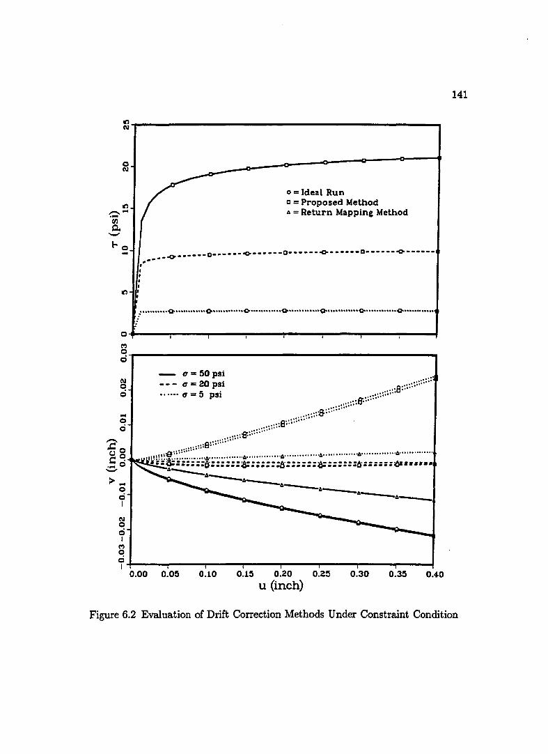
~,---------------------------------------------------~
o C\I
It')
-.'" .... (fJ
0. -too ...
0
M 0 ci
C\I 0 ci
... 0 ci
Z ",0 c;:C!
.... 0 -> ... 0 c:i I
C\I 0 c:i I
M 0 ci I
0= Ideal Run a = Proposed Method A = Return Mapping Method
.--.. ~ ______ D ______ ~ ______ D _____ .~ ______ D __ • __ .~ __ • __ •
• • •
/ ........... Oo ............ Oo ............ Oo ............ Q ............ ·Qo ••• •• .. • .. ··OO·· .... ······OO .. •· .. · .... ·
- q=50psi - - - q = 20 psi ...... q = 5 psi
0.00 0.05 0.10 0.15 0.20 0.25 0.30 0.35 0.40 u (inch)
141
Figure 6.2 Evaluation of Drift Correction Methods Under Constraint Condition

142
this reason, the results obtained from the ideal run can be thought to be the exact
solution. Therefore, to examine the performance of the algorithms, the results
obtained from the proposed method and the return mapping algorithm can be
compared with the ideal run. Since the aim here is to compare the performance
and accuracy of the algorithms, the results obtained from these three methods are
not compared with the experimental data in Fig.(6.2).
The experiment involves shearing two concrete blocks, whose contact surface
is fiat (no asperities), under direct shear condition with constant normal stress. At
a given shear displacement, u, the shear stress, T, and normal displacement, v, of
the concrete joint are measured. The test is performed for three constant normal
stresses t7 =50, 20 and 5 psi (345.6, 138.2 and 34.6 kPa). Since the contact surface
is fiat, measured normal displacements are virtually zero in all three cases.
The constitutive model proposed by Fishman (1988), and Desai and Fish
man (1988) for rock joints is used herein to back predict the experimental data.
This model utilizes the same yield function (Eq.4.11) and potential function
(Eq.4.14) with progressive hardening. No damage is considered, but a and aQ
are defined as a = a e6 and aQ = a + 11:( ai - a )(1- sr). The parameters used are;
n = 2.5, "y = 0.36, a = 0.02312, b = -0.116, II: = 0.7 and
Ks = 4000psi/inch (10.9 x 10⁻⁶ kPa/m).
The constitutive Eq.( 4.20) is integrated numerically using Euler's first first
order explicit method (ideal run), proposed method and return mapping algorithm.
During the numerical integration, 0- = 0 and v :F 0 are the constraint conditions
applied to Eq.( 4.20). Since the proposed method can handle the constraint case, it
should perform well to prove its capability. The return mapping algorithm in not
suitable for such constraint condition, however, by imposing if = 0 and v = 0, the
equations are suitably modified to handle this situation.
Figure (6.2) shows comparison of results obtained from the proposed
method, return mapping algorithm and ideal run. The ideal run is performed
with du = 0.00001 inch and a total of 40000 steps. The proposed method and the
return mapping algorithm use step size du = 0.1 inch and a total of 40 steps.

143
Evidently all the three methods give the same shear stress, however; the
normal displacement calculated by the return mapping algorithm differ from that
of the ideal run and the proposed. Since general agreement is observed between the
ideal run and the proposed method in both shear stress and normal displacement
for all normal stresses, it can be concluded that the proposed method performs
well. It is found that the proposed method requires an average of 2 iterations per
step, whereas the return mapping algorithm requires 7 iterations per step. It is also
found that when du = O.linch, the proposed method gives almost same prediction
as that of du = O.Olinch. For this condition, on the other hand, the return mapping
algorithm gives almost sam~ shear stress but different normal displacement. From
the view point of average number of iterations per step and sensitivity of step size,
the proposed method proved to be efficient.
6.5 Stability Analysis
Stability is a very important characteristic for numerical integration in initial
value problems. Stability in a system implies that small changes in the system
inputs, in intial conditions or in system parameters will not result in large changes in
the system behavior. In the context of a numerical integration algorithm, stability
is a necessary and sufficient condition for convergence as the step size is allowed
to tend to zero (Ortiz and Popov 1985). The question of stability of the proposed
algorithm is dealt with in this section.
In a stable linear time-invariant system;
(1) with bounded input, the output is bounded,
(2) with zero input and with arbitrary initial conditions, the output tends to-
wards zero, that is, - the equilibrium state of the system.
The first notion of stability concerns a system under the influence of inputs and
the second notion concerns a free system relative to its transient behavior. These
two notions of stability are essentially equivalent in linear time-invariant systems.
In nonlinear systems, there is no definite correspondence between the two notions.
For a free stable nonlinear system, there is no guarantee that the output will
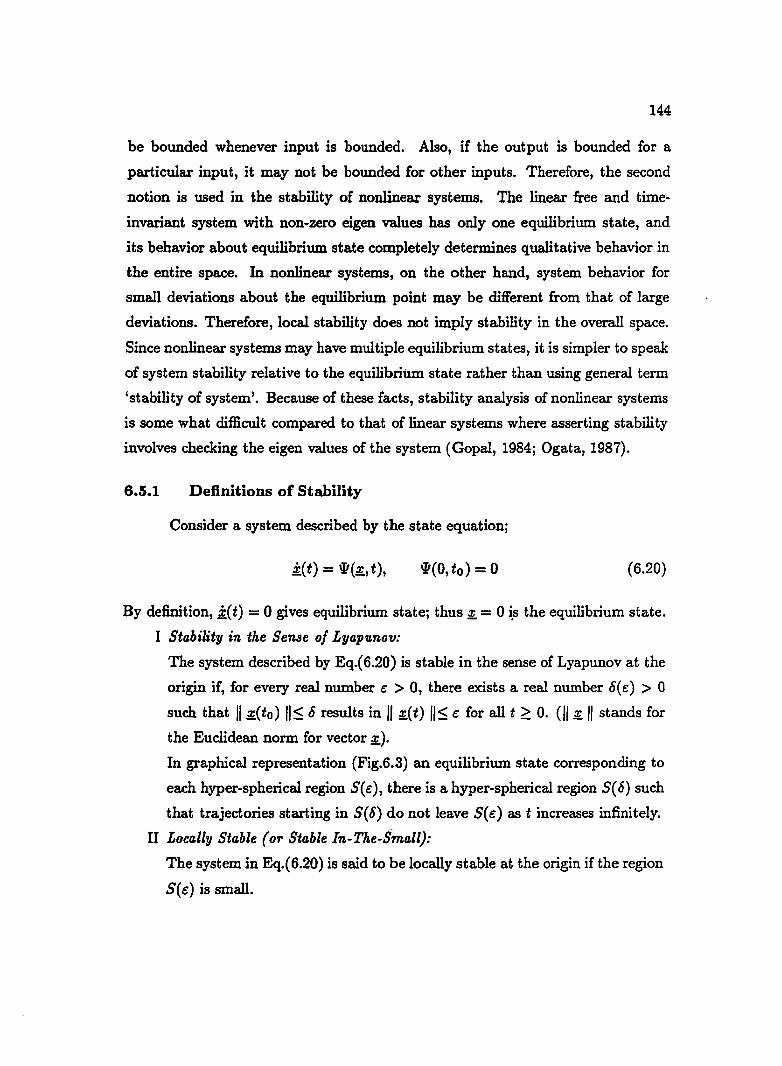
144
be bounded whenever input is bounded. Also, if the output is bounded for a
particular input, it may not be bounded for other inputs. Therefore, the second
notion is used in the stability of nonlinear systems. The linear free and time
invariant system with non-zero eigen values has only one equilibrium state, and
its behavior about equilibrium state completely determines qualitative behavior in
the entire space. In nonlinear systems, on the other hand, system behavior for
small deviations about the equilibrium point may be different from that of large
deviations. Therefore, local stability does not imply stability in the overall space.
Since nonlinear systems may have multiple equilibrium states, it is simpler to speak
of system stability relative to the equilibriUm state rather than using general term
'stability of system'. Because of these facts, stability analysis of nonlinear systems
is some what difficult compared to that of linear systems where asserting stability
involves checking the eigen values of the system (Gopal, 1984; Ogata, 1987).
6.5.1 Definitions of Stability
Consider a system described by the state equation;
i(t) = \II(~, t), \11(0, to) = 0 (6.20)
By definition, i(t) = 0 gives equilibrium state; thus ~ = 0 i.s the equilibrium state.
I Stability in the Seme of Lyapunov:
The system described by Eq.(6.20) is stable in the sense of Lyapunov at the
origin if, for every real number e > 0, there exists a real number «5( e) > 0
such that "~(to) 11:5 «5 results in II ~(t) 11:5 e for all t ~ O. (II ~ " stands for
the Euclidean norm for vector ~).
In graphical representation (Fig.6.3) an equilibrium state corresponding to
each hyper-spherical region See), there is a hyper-spherical region S( 6) such
that trajectories starting in S(5) do not leave See) as t increases infinitely.
II Locally Stable (or Stable 111.- The-Small):
The system in Eq.(6.20) is said to be locally stable at the origin if the region
See) is small.

S(~, SIft
c.) eb) ee)
Figure 6.3 (a) Stable Equilibrium State and a Representative Trajectory; (b) Asymp
totically Stable Equilibrium State and a Representative Trajectory; (c) Un
stable Equilibrium State and a Representative Trajectory. (Orgata, 1987)
I-' tJ:>. C1t

146
III A"ymptotically Stable:
The system in Eq.(6.20) is asymptotically stable at the origin if it is stable in
the sense of Lyapunov and if every solution starting within S( 8) converges,
without leaving S( e), to origin as t increases indefinitely.
IV A"ymptotically Stable In-The-Large (or Globally Asymptotically Stable):
The system in Eq.(6.20) is asymptotically stable in-the-Iarge at the origin
if it is stable in the sense of Lyapunov and if every solution converges to
origin.
V Instability:
The system in Eq.(6.20) is instable at the origin if for some real number
e > 0 and any real number 8 > 0, no matter how small there is always a
state ~( to) in S( 6) such that the trajectory starting at this state leaves S (e).
The proposed algorithm falls under the category of nonlinear discrete-time
autonomous system (an autonomous system is one that is both free and time
invariant). Lyapunov's direct method is the most powerful technique available
today for the stability analysis of nonlinear systems. It is cautioned, however,
that although Lyapunov's direct method is applicable to any nonlinear system,
obtaining sucessful results may not be an easy task. Experience and imagination
may be necessary to carry out stability analysis of most nonlinear systems. In
what follows, a brief statement of Lyapunov's stability theorem for discrete-time
autonomous system is presented. Subsequently using this theorem, stability proof
of the proposed algorithm is presented.
Direct method of Lyapunov is based upon the concept of energy and the
relation of stored energy with system stability. IT the system has an asymptotically
stable equilibrium state, then the stored energy of the system displaced within a
domain of attraction, (S( e), Fig.6.3), decays with increasing time until it finally
assumes its minimum value at the equilibrium state. For some systems, there is
no obvious ways of associating an energy function with a given set of equations
describing the system. In this case, a non-negative scalar function (V(x» of sys
tem state, known as Lyapunov function, can be employed in the investigation of

147
stability. Now consider a nonlinear autonomous discrete-time system
q,(0) = 0 (6.21)
where, i indicates the time step. By definition, the equilibrium state is given by
~(i + 1) = OJ thus ~ = 0 is the equilibrium state.
6.5.2 Lyapunov's Stability Theorem
For the autonomous system (6.21), the sufficient conditions of stability are
as followsj
Suppose there exists a scalar function V(~(i)) which, for some real number
e > 0, satisfies the following properties for all ~ in the region II ~ /1:5 e:
(1) V(~) > OJ ~ rf 0
(2) V(~) = OJ ~ = 0
(3) V(~) is continuous for all~.
Then the equilibrium. state of L = 0 of the system (6.21) is
(a) Stable if the difference computed along the system trajectories, b. V(~(i)) =
V(~(i + 1)) - V(~(i)) :5 OJ
(b) AJymptotically Jtable if b.V(~(i)) < 0, ~ rf 0 or if ~V(~(i)) :5 0 and
~ V (~( i)) is not identically zero on a solution of difference Eq. (6.21) other
than~= O.
(c) Globally aJymptotically Jtable if the condition of asymptotic stability hold
for all ~ and, in addition, V(~(i)) -+ 00 as II ~ 11-+ 00.
6.5.3 Stability Proof
ten as
or
From Eq.(6.19a), the goverening equation of the proposed algorithm is writ-
• i+l _ .T,( i ) 1Z:n + 1 = "If 1Z:n + 1
(6.22a)
(6.22b)
148
Notice that Q~11 is related to £~~l via Eq.(6.16). Hence the algorithm has only one
independent variable, and £ is chosen as the independent variable in the analysis.
Now, observe that the equations (6.21) and (6.22) are similar.
The aim of the iteration technique is to make 1(!Z.~"tll' o~"t\) = 0. In gen
eral, at ith iteration step 1(!Z.~+1' 0~+1) > O. Since Lyapunov function is usually
considered to be an energy function of the system, the yield function I(!!., 0) pos
sess suitable properties to be a candidate for a Lyapunov function. Therefore, the
following function is chosen as Lyapunov function;
V(!l., 0) = P 1(!Z.,0) (6.23)
where p is a positive constant. Observe that the initial condition is given by
(£~+1' O~+l)' The correct solution obtained after m number of drift correction
iteration is the equilibrium state *e = (!Z.n+1,On+1)' When !Z.~+1 remains outside
of the yield surface N i Ni, 1(!!.~+1' 0~+1) > 0. It is required that the system
Eq.(6.21) exhibits \11(0) = 0, and ~ = ° is the required equilibrium point. To this
end, a transformation of origin of stress space from (0,0) to the equilibrium point
(£n+1,on+d is performed via
i -i + !Z.n+ 1 = !Z.n+1 !!.n+ 1
0~+1 = 1i~+1 + On+l
(6.24a)
(6.24b)
will take f(!!.~+1' O~+l) as a non-negative quantity, and at equilibrium point
1(£n+l,On+l) = O. With the above, the dynamical system Eq.(6.22) has a set
of state variables defined by (~, Ii) with the equilibrium being at the origin of the
state space. Observe that the functional value of I(!!., 0) is not changed due to the
transformation. Thus the scalar function V(!Z., 0) is positive definite;
V(Q, 0) = ° (6.25a)
(6.25b)

149
The yield function I is continuous in (.~, &) space. Thus V (£, a) is continuous for
all (.~, &). Assuming p = 1, and computing l:::. V;
Using Eq.(6.16); Av.i (01) . i+1 (01) . i+l u n+l::::: O!l. !l.n+l + OQ Qn+l
Computation of l:::.V along the system trajectories Eq.(6.19a) results in;
(6.26)
Here in Eq.(6.26):
(1) A > 0 if 1(!l.~+I' Q~+1) > O. i.e the stress point lies out side of
the yield surface.
(2) For hardening material [ (~)Tce(~) - H] is always positive.
(3) At equilibrium 1(!l.~+1' a~+I) = o. Thus, if stress point (!l.~+1,Q~+1) lies out side of the yield surface NiNi, l:::.V~+1
is negative definite except at the equilibrium point. It is also to be noted that
V(£, a) = I(B=., a) is positive for all values of (~, &) except at the equilibrium point.
Therefore, by Lyapunov's stability theorem, the system is globally asymptotically
stable. The stability of the dynamical system Eq.(6.22a), proved above, guarantees
that the algorithm Eq.(6.22a) will converge to (!l.n+l' an+d from the initial value
(~n' an). Furthermore, the stability analysis by the Lyapunov method gives only
sufficient conditions, which are usually overly restrictive for nonlinear systems. This
implies that the algorithm can also be stable in many different practical situations
where some of the restrictions imposed in the analysis are not met.
6.6 Further Considerations on Drift Correction
Two interesting features such as (1) negative drift and (2) drift correction at
small!l. (or J1 ) need special attention while employing the drift correction methods
presented in Sections 6.2 and 6.3. These two aspects are dealt with in this section.
150
6.6.1 Drift Correction for Negative Drift
Figure (6.4a) shows the position of stress point Bi and yield surface NiNi
obtained at the end of i th iteration during drift correction. Since Bi lies out side
the surface Ni N i , this condition indicates positive drift, i.e f(!l.~H' a~+l) > O.
During the process of drift correction, the yield surface moves (outwards) towards
stress point and stress point moves (inwards) towards yield surface, thereby re
ducing the drift monotonically until reaching the correct state. When the drift is
positive, a stable algorithm guarantees convergency.
During the drift correction iterations, it is possible that the drift can be
negative. Figure (6.4a) shows the occurance of negative drift at the end of ( i + 1) th
iteration. Here, the stress point Bi+l and yield surface Ni+l NiH are obtained at
the end of (i + l)th iteration. Since Bi+l lies out side of surface Ni+l NiH, this
condition indicates negative drift, i.e f(fI:.~t\, a~~l) < O.
This situation could have arisen due to excessive correction applied to both
£~~11 and Q~tll so that the updated yield surface Ni+l NiH moved to far outwards
and updated stress point Bi+l moved to far inwards. In order to bring stress
point BiH to the yield surface NiH Ni+l, this surface has to be moved towards
NiNi and point Bi+l has to be moved towards Bi. Moving the surface Ni+l NiH
towards surface N i N i means that the Q~~ll should be positive. But, during drift
correction the generated plastic strain f~~tl could be either positive or negative,
nevertheless it will always produce negative Q~tl1' Thus, the surface Ni+l NiH
always moves away from Ni Ni.
The drift correction theory presented in Sections 6.2 and 6.3 is generally
valid for positive drift (f(!l.~~l' a~~l) > 0) case. Still, it had been shown (N avayo
garajah, 1988) that this theory is valid for negative drift case provided the a~~ll is
suitably modified.
Based on the above information, negative drift correction case requires spe
cial attention and needs new class of algorithm other than the ones used for positive
drift correction. Detail treatment of this aspect can be found in N avayogarajah
(1988). Compared to some of the rigorous and theoretical!y appealing algorithms,

(a) Negative Drift
o~ ______________________ ~ ______________ ~--,
• a
Ul timate /# .. o \ .......... ..
M L-____ ----~F~=~5~0~----------~--------~ .... ~ .. ~ .. -.. --
I .... .. r .... I
..
...... .... ".-#
.. ..
10 .......... X : Phase Change ~ .. ' .. ' ..
.. ." ." " .--
o ... 1-_--a
o~~~~~----~------~------~--~~,~--~ o 10 20 30 40 50 60 (j (kPa)
(b) Drift Correction at Small Normal Stress (or J1 )
Figure 6.4 Comments on Drift Correction Algorithms
151

152
an approximate but simple algorithm, where bringing stress point ni+l to C (lies
on surface NiH NiH) elastically along the incremental stress direction Bi Bi+l to
the yield surface NiH NiH, yields sufficiently accurate results. Observe that this
method is approximate since the associated strain (plastic) is not considered in the
calculation when stress point moves from Bi+l to C.
6.6.2 Drift Correction at Small Normal Stress (or J1 )
It is observed that the drift correction methods presented in Section 6.2
converges slowly when normal stress 0' (or J1 ) is small; in other words the stress
points lie in the region left of line aa in Fig.( 6.4b). Moreover, during the numerical
integration of Eq.( 4.20) for constant normal stress, the drift correction methods
are found to converge slowly only at the very first step, and afterwards, its conver
gency rate is fast as usual. A simple method is presented herein to over come this
difficulty.
Keeping a constant for various values of A, the yield function 1(0', T, a) = A
(Eq.4.11) gives family of yield curves as shown in Fig.( 6.4b). Line aa is obtained by
connecting phase change points on all the yield curves and aa is parallel to Taxis.
The family of curveI'! 1 = A have almost same curvature as that of 1 = 0 curve
in the right side of line aa. In the left region of line aa, on the other hand, the
curves are becoming almost parallel to 0' axis at higher A values. This makes the
quantities (~) and (*) calculated for example at point X very small compared
to (fJfl:) or (~), and consequently small contribution of these terms to the drift
correction (see Eqs.6.11 to 6.19) results in normal stress if being corrected slowly
and the iteration converges slowly. The algorithm is extremely slow in this region
for a dilating material with non-associative rule due to the fact I~I < 1*1. Among the possibilities explored (Navayogarajah 1988), it is found the fol
lowing method is easy to implement and gives satisfactory results. Calculate (~)
and (~) at point X using an yield curve J(~x' ax) = 0, passing through the point
X. In this method, O'x is known, and using the yield function (Eq.4.11) ax can
be computed (when the point X located above failure line, ax will be negative. In
this case use ax = 0). In summary, first check if 0' falls in the region left of line

153
aa. IT so, compute (~) and (~) as explained before and use these quantities in
the drift correction equation presented in section 6.2.
6.7 Comments
The proposed drift correction method for constraint condition is shown to
be efficient and stable. As shown before, the proposed method produces correct
projecting back method as special case under total constraint of i. Implementation
of the proposed method for the interface under constant normal stress is revealed.
Generality of the proposed algorithm is due to the fact that it is formulated based
on response function of material and not based on particular type of constitutive
models.
During drift correction, negative drift should not occur when a stable algo
rithm is used. However, in such event, a simple method is presented to circumvent
this problem. Slow convergence of algorithm for small (j can be attributed to
the type or geometry of yield function employed rather than the performance of
algorithm.

154
CHAPTER 7
FINITE ELEMENT METHOD FOR INTERACTION PROBLEMS
A crucial assumption in the development of theoretical solution to interac
tion problem concerns the frictionless behavior at contact zone. Such assumption
of theoretical convenience deviates considerably from realistic behavior of contacts
or interface where friction forces play vital role. Due to the relative motions and
friction at the interface, theoretical analysis of soil-structure interaction problems
become intractable, even in the case of simple elasto static problems. Numerical
methods of stress analysis, such as finite element method, finite difference method
and boundary element method, seem to be viable approaches to the solution of in
teraction problems. The use of high speed and large memory digital computers has
made numerical approaches feasible and economical, and therefore, more attractive
to practicing engineers and researchers.
The presentation of this chapter is divided into two sections namely: (1)
brief review of available solution techniques for soil-structure interaction problems,
and (2) finite element formulation for dynamic interaction problem.
7.1 Solution Techniques for Soil-Structure Interaction Problems
Analysis of soil-structure interaction problem must account for factors such
as (1) non linear properties of soil and structure, (2) semi-infinite domain of the
soil, (3) proper model for interface, (4) complex nature of wave propagation in soils,
(5) presence of neighbouring structures, and (6) three-dimensional nature of the
problem. Such an analysis is complex and some form of idealization of the problem
is required in order to simplify the complexity involved. Usually a soil-structure
interaction problem is simplified, as described by Idriss et al. 1979, by making
suitable assumptions such as (1) replacing infinite soil domain by a finite domain,
(2) seismic input in the form of force or displacement applied at boundaries in
155
certain direction, and (3) simplified behavior of the interfaces. Such simplified
interaction problems can be solved in practice.
Solution procedure of the simplified interaction problems can be broadly di
vided into two classes: (1) analytic or continuum method and (2) numerical method
(Wolf, 1985). The analytic method is suitable only for simple problems such as fric
tionless interface, linear material behavior and simple loading and boundary condi
tions. A numerical method can incorporate complex geometry, complex boundary
condition, complex loading, nonlinear material behavior and interface characteris
tics.
Numerical methods for solution to interaction problem are divided into three
classes: (1) multi-step method, (2) substructure method, and (3) direct method.
Among these methods, attention is focused on the direct method. In the direct
method, the response of the structure and soil is evaluated in a single analysis
step. The equations of motion resulting from the formulation of soil-structure
system can be solved in the time domain or in frequency domain. The frequency
domain solution is limited to linear analysis, whereas time domain solution can
handle material, geometric and boundary non linearities.
Though the finite element method is versatile in the solution of dynamic soil
structure interaction problem, yet it can not simulate the condition of semi-infinite
extent of the soil. Several methods are proposed to overcome this problem such as
(1) using absorbing boundaries using viscous dampers at the soil boundaries, and
(2) using infinite elements.
In this study, the direct method of solution to soil-structure interaction
problem using finite element method is adopted. Figure (7.1) shows a typical finite
element discretization for two dimensional finite element analysis of a soil-building
system shown in Fig.(1.1c). The soil, structure and interface elements are shown
in this figure. As discussed before, for the dynamic analysis, the infinite domain of
soil is replaced by a finite domain with absorbing or transmitting boundary. Now
the finite element formulation for dynamic analysis of soil-structure interaction
problem is presented below.

Superposition Boundary
Structural Elements
Soil Elements
~ ~ ~ ~~~,f,' 'F ~ LjJ
Viscous Dashpots
Time Time
Cyclic Load Earthquake Load
Figure 7.1 Finite Element Idealization of Soil-Stnlcture Interaction Problem
156

157
7.2 Finite Element Formulation
7.2.1 Solution of Governing Equation of Dynamic Problems
The solution of dynamic problems for nonlinear physical and geometric prop
erties require use of numerical procedure that involve two phases: (1) discretization
in space, and (2) advancing the solution in time domain. In the finite element for
mulation, displacement field is assumed in the form
{u} = [N]{q} (7.1)
where {u} is the displacement vector of a point in the element, [N] is the matrix
of shape function and {q} is the unknown nodal displacement vector. The strain
vector {f} can be written as
{f} = [B]{q} (7.2)
where [B] is the standard strain-displacement transformation matrix (Bathe, 1984).
Employing the Eqs.(7.1) and (7.2), the virtual work equation of a body under
dynamic motion is approximated, and the resulting spatial discretization leads to
the following system of ordinary second order differential equations:
[M]{q} + [C]{q} + {P} = if} (7.3a)
where
[M] = j[NV p [N]dV (7.3b)
v
[C] = j [Nf c [N]dV (7.3c)
v
{P} = j[BV {q }dV = j[Bf[CeP][B]dV {q} = [K]{q} (7.3d)
v v
[K] = j[B]T[CeP][B]dV (7.3e)
v
if} = j[NjT{X}[N]dV + j[NjT{T}dS (7.3!)
v s
158
where, [M] is the mass matrix, [C] is the damping matrix, [K] is the stiffness
matrix (tangent), {P} is the vector of internal resistance of the system that opposes
deformation of the body, {f} is the vector of externally applied loads, {X} is the
body force per unit volume, {T} is the traction vector acting over the surface S;
over dot denotes time derivatives. Here, p is the mass density per unit volume and
c is the damping coefficient.
In this study an 8-noded isoparametric element is used as soil and structure
element, and 6-noded isopara-linear element is used as interface element. Formu
lation of interface element is given in Chapter 8. The mass, damping and stiffness
matrice (Eqs. 7.3b, 7.3c and 7.3e) are evaluated numerically using two point (2 x 2)
or (3 x 3) point integration of Gauss method.
7.2.1.1 MElSS Matrix
The mass matrix given in Eq.(7.3b) is called consistent mass matrix and it is
fully populated. However a diagonal mass matrix, which is also known as lumped
mass matrix, is desirable as storage space and computation time is reduced in
implicit time integration scheme. It is proved that the solution of dynamic problems
using lumped mass matrix is convergent if total mass of the element is preserved.
Such lumped mass matrix is obtained by lumping the mass in proportion to the
diagonal terms of the consistent mass matrix. The diagonal terms of lumped mass
matrix given by
MT= J pdV v
(7.4a)
(7.4b)
where MT is the total mass of the element and Mfi is the diagonal term in the
consistent mass matrix Eq.(7.3b).
7.2.1.2 Damping Matrix
Two types of damping can be identified in the dynamic behavior of materials,
namely (1) viscous and (2) hysteretic damping. The energy loss in viscous damping
is proportional to the velocity and it is frequency dependent. Due to friction, energy

159
is lost in hysteretic damping and it is independent of frequency but dependent
on the magnitude of the displacement. As explained in Chapter 4, elasto-plastic
materials exhibit hysteritic damping via hysteresis stress-strain loops and the area
of the loop is directly proportional to energy loss in the material.
For linear analysis, as the damping properties are frequency dependent, it
is difficult to determine damping parameters that can be used in the formulation
of [C] matrix. Rayleigh damping coefficients a and (3 are used to construct [C]
matrix from the mass matrix [M] and the stiffness matrix [K] of the complete
element assemblage as following
[C] = arM] + f3[K] (7.5)
The [C] matrix constructed by this method is easy to incorporate in computation.
For nonlinear analysis, hysteritic damping directly comes from the hysterisis loop
of the elasto-plastic material.
7.2.1.3 Stiffness Matrix
The soil behavior is modeled using 81 model for nonassociative behavior in
the hierarchical single surface approach, and linear elastic model is used to simulate
the structure. Details of 81 model are given in Appendix A. Using appropriate
constitutive matrix, the stiffness matrix (Eq.7.3e) can be constructed. Formulation
of stiffness matrix for interface element is given in Section 8.1.
7.2.2 Time Integration
Time integration is usually performed by employing finite difference schemes
which force the goverening equations to be satisfied at selected nodal points along ,
time coordinate. Accuracy and efficiency of solution of time dependent problems
are significantly influenced by the time scheme employed. The time integration
schemes are broadly classified as explicit schemes, implicit schemes and mixed
methods. Implicit schemes are unconditionally stable for linear analysis, if suit
able parameters are selected. However, for nonlinear problems, implicit schemes
may not necessarily be stable, but permit the use of larger time steps compared to

160
explicit schemes. Unfortunately implicit schemes require matrix factorization that
involve larger computer core storage and more operation per time step compared to
explicit schemes. The mixed or implicit-explicit methods offer a unified approach
to problems of transient dynamics and can lead to significant computational ad
vantages (Owen and Hinton, 1980).
The initial value problem posed by Eq.(7.3) consists of finding {q} at time t,
satisfying Eq.(7.3) and prescribed initial conditions. A number of implicit schemes
are available, but the discussion here is limited only to Newmark's implicit scheme.
7.2.2.1. Newmark's Implicit Time Integration Scheme
Time domain is divided into time steps and the solution at time t+l = t+~t
is obtained by considering equilibrium at time t + 1. {qt}, {qt} and {qt} represent
the displacement, velocity and acceleration at time t, respectively. The problem
consists of finding the values {qt+l}, {4t+!} and {qt+!} at time t + 1 once their
values at time t is known. If the matrices [M], [C] and [K] do not change with
time, the general procedure of time integration is written as
{qt+l} = ,8~t2 {~qt+l} - ,8~t {qt} + (2~ _1){qt}
{4t+!} = {4t} +~t(I-1'){qt} +1'~t{qt+l}
{qt+l} = {qt} + {~qt+l}
(7.6)
(7.7a)
(7.7b)
(7.7e)
where ~t is the time step size; ,8 and l' are the parameters which govern accuracy
and stability of the scheme. It has been shown, when 2,8 ~ l' > 1/2 the scheme is
unconditionally stable, and when l' > 1/2 and ,8 < 1'/2 the scheme is conditionaly
stable with restriction on time step.
Using the following expression for equivalent· nodal force vector {pt+!};
(7.8)

161
with Eqs.(7.7) and (7.8) in Eq.(7.6) one obtains;
(,8~t2 [MJ + ,8~t[CJ + [[(J) {~qHl} =[MJ(,8~t {qt} + (2~ -1)Ur})
+ [CJ((1' _1){qt} + ~\1' _ 2){qt}) {J 2 {J
+ {fHI} _ {pt} (7.9)
This set of equation is solved for {~qHI}, then acceleration and velocity are com
puted using Eqs.(7.7a) and (7.7b) respectively. Members of the family of Newmark
scheme is obtained for various set of values for l' and,8. When l' = 1/2 and,8 = 1/4
the scheme is unconditionally stable and this member of the family has most de
sirable accuracy compared to other members. In this study, l' = 1/2 and ,8 = 1/4
are the values used.
7.2.3 Non-Linear Solution Techniques
Because of the assumption of linearity of various quantities in time step 6.t,
the solution of Eq.(7.9) is approximate, thus the calculated stresses will not satisfy
equilibrium. Therefore, iterations within each time step are necessary to satisfy
equilibrium at the end of time step. Some of the most generally used methods are
incremental method, Newton-Raphson or Iterative Newton-Raphson method, ini
tial tangential stiffness method, initial stiffness method and mixed methods (Desai
and Abel, 1972). Newton-Raphson method is adopted for the solution of Eq.{7.9).
7.2.4 Convergence
Iteration of Eq.(7.9) for a given time step has to be terminated based on con
vergency criteria. The convergency criteria can be established based on three types
of variables, namely; deflection, residual force and step-by-step internal energy. In
this study, convergency based on residual force is employed. In this criteria, the
Euclidian norm of the residual (out-of-balance) force vector should be kept within
a tolerence of a reference load increment.

CHAPTERS
APPLICATION OF INTERFACE MODEL IN
BOUNDARY VALUE PROBLEMS
162
The aim of developing a constitutive model is not limited to the prediction
of laboratory test data, but to successfully utilize it in the solution of boundary
value problems. Validity and robustness of a constitutive model can be checked
by adopting it in the solution of boundary value problems using the finite element
method.
The interface model developed in Chapter 4 is implemented in a general pur
pose dynamic finite element program developed by Desai (1989) to solve dynamics
of an axially loaded pile. Implementation of the model in the above problems is
treated in detail in this chapter. This chapter is divided into two parts: the first
part deals with the representation of interface element in the finite element method,
and the second part contains the application of interface model to boundary value
problems.
S.l Finite Element Representation of Illterface Element
The thin layer element (Section 2.3.1) proposed by Desai et al. (1984) is used
here to simulate the interface in the finite element method. Further development
on the thin layer element such as inclined interface and incremental elasto plastic
stress-strain relation are considered in this section. Some of these aspects can be
found in Sharma and Desai (1990). Figure (2.1a) shows a typical two dimensional
thin layer interface element and sorrounding continuum elements. The interface
element has a thickness t and length B. Figure (B.1a) shows the interface element
inclined by an angle () to the global coordinate system (X, Y). The coordinate
system (x, y) is such that it is parallel (T) and normal (N) to interface plane, thus
the a."Cis system (x,y) is called local coordinate system. This.section deals with the

y
x
(x,y) -- Local Coordinate System (X,y) -- Global Coordinate System
(a) Orientation of Interface Element with Respect to
Global Coordinate System
Y(Nl
L 1]
6 5 4
+ +
x{T) + +
1 2 3
(b) Six-Noded Interface Element in Natural
Coordinate System (e, 1"/)
Figure 8.1 Inclined Interface Element
163
164
formulation of stiffness matrix for the interface element. In order to achieve this, in
the first part, incremental stress-strain relation for the interface behavior is formu
lated in the local system (x, y) and the stiffness matrix is formulated in the same
system. The second part describes the detail of the transformation law required
for an inclined interface element to calculate stiffness matrix and unbalanced load
vector.
The interface element is represented by a "thin" isopara-linear six noded
solid element as shown in Fig.(8.1a). Such thin element has a higher aspect ratio
(length/thickness, B It) with constant strain in the thickness (y(N)) direction and
linear variation of strain along the length (x(T» of interface element (Desai and
Nagaraj, 1989). This type of strain variation represents simple shear condition
(Fig.4.1c) which is compatible with the assumption of two dimensional idealization
of the interface. Use of six noded element, insted of 8 node, prevents occurance
of ill conditioning in interface element by avoiding the mid node in the thickness
direction.
Employing the shape functions for 6 noded element in natural coordinate
system (e, 7]), incremental displacement vector of the interface element {du} can
be written as
{du} = [N]{dq} (8.1)
where [N] is the matrix of the shape function and {dq} is the incremental nodal
displacement of the interface element. Using the isoparametric concept, the incre
mental strain vector {de} can be written as
{ de} = [B]{ dq } (8.2)
where [B] is the standard incremental strain-nodal displacement transformation
matrix.
Plane strain condition is assumed herein to illustrate the finite element for
mulation. In this case;
(8.3)

165
8.1.1 Incremental Stress - Strain Relation for Interface
The incremental form of elasto-plastic constitutive relation for interface is
given by
{ du xx } [0 0] { . } duyy = Cnn Cns ~ duxy Csn Css
( 4.20a)
or
( 4.20b)
In Eq.( 4.20), the incremental stress and incremental displacement are related
through elasto-plastic matrix [Cep*]. Assuming simple shear strain condition, the
incremental displacement-incremental strain are related via
{den} [0 0] { . } de yy = lit 0 ~ dexy 0 lit
(S.4)
where t is the thickness of interface element. Combining Eqs.(S.4) and (4.20);
(S.5a)
or
[dO'] = [cep*] [de] (S.5b)
Because of two dimensional idealization of the interface, the yielding characteristics
of the interface is independent of dO' xx, thus zero value is assigned for dO' x x' As
seen from Eq.(S.5a), the incremental normal stress on the interface (dO') is given by
du yy and the incremental shear stress on the interface (dr) is given by dO' xy' The
elasto-plastic matrix [cep*] in Eq.(S.5) is used in the finite element formulation to
compute stiffness matrix (Eq.7.3e) of the interface element.

166
8.1.2 Transformation from Global Space to Local Space and Vice Versa
Very often an interface element can be inclined to global axis (X, Y), Fig
(B.1a), in many boundary value problems. The interface behavior (Eq.4.20) is
originally defined as the constitutive relation between incremental traction force
vector and incremental displacement vector refered to axes parallel and normal
to the interface plane (x, y) in Fig.(B.1a). Subsequently, Eq.( 4.20) is conveniently
inverted into incremental stress-strain form given by Eq.(8.5) which can be readily
used in the finite element formulation of interface. Since the traction forces (or
stress) and displacements (or strain) of interface plane depends on the orientation
of interface plane (x, y), for an inclined interface element, transformation of stress
and strain from local system (x, y) to global system (X, Y) or vice versa is necessary.
The transformation is required at two instances; (1) calculation of global stiffness
matrix of interface element, and (2) calculation of unbalanced load vector during
iteration for convergency. The steps involed in the transformation is explained
below.
The transformation of strain vector and stress vector from local to global
description is given by;
[dE] = [,8][de]
[dS] = [,8'][dq]
Similarly the transformation from global to local description is given by
[de] = [e][dE]
[du] = [6'][dS]
where
[PI = [~ cs -cs ] ~'l = [~
C8 -2~ ] c2 cs c2 2cs
-2cs c2 _ 82 -cs c2 _ 82
[ 0 0
o ] [ 0 0 -~cs ] [e] = s2 c2 -cs [e'] = S2 c2
-2cs 2cs c2 _ 82 -cs cs c2 _ s2
(B.6a)
(B.6b)
(S.7a)
(S.7b)
(B.Sa)
(S.Sb)
and the vectors in global description is given by
< dET > = < dExx, dEyy, dExy >
<dST > = <dSxx,dSyy,dSxy >
and local description is given by
< deT > = < deu , deyy , d",/zy >
< dO'T > = < dO'zz, dO'yy, doozy>
167
(S.9a)
(8.9b)
(8.lOa)
(8.10b)
Also c = cos{} and s = sin{} and {} is the inclination of (x, y) with the respect t<,>
(X, Y) as shown in Fig.(S.la). Notice that the zeros in the first column of [,8] and
[,8'] and zeros in the first row of [e] and [e'] is due to deu = 0 and dO' xx = 0,
respectively.
To establish global stiffness matrix for interface element, consider the incre
mental force vector {P}, Eq.(7.3d), that opposes the displacement of the structure
{P} = j[Bf idS }dV (7.3d)
V
Observe that Eq.(7.3d) is global description, and combining Eqs.(7.3d), (8.6b) and
(S.5b) one obtains:
{P} = j[Bf[Cep]{dE }dV (S.lla)
v
where
(8.12)
The matrix [Cep] can can be conveniently incorporated as the constitutive matrix
of the inclined interface in gobal description and Eq.(S.12) gives the transformation
rule. The global stiffness matrix for an inclined interface element can be computed
using the [Cep] given by the Eq.(S.12). Hence, for an inclined interface element,
mass, damping and stiffness matrices [M], [C] and [K] are calculated and assembled
in global system (X, Y) and the solution of Eq.(7.9) is obtained in the same system.
168
In the case of a material non-linear problem, it is necessary to compute the
unbalanced load vector Iv [B]T {dS }dV in all the elements of the mesh during iter
ation in order to equilibrate the externally applied loads. During the calculation of
unbalanced load, for the calculated global incremental strain {dE}, the correspond
ing change in global stress {dS} is to be computed using the constitutive relation.
For the inclined interface element it is achieved by transforming global incremen
tal strain {dE} to local incremental strain {de} using Eq.(8.7a) then applying the
constitutive relation given by Eq.(8.5), the local {dO'} is calculated. Finaly, the
local {dO'} is transformed to global {dS} using Eq.(8.6b). Now the {dS} is used to
compute the unbalanced load in the global system.
8.2 Dynamics of Axially Loaded Pile
Performance of the proposed interface model in boundary value problems
is'demonstrated by applying it to dynamic analysis of an axially loaded pile. The
suitability of this problem is due to the fact that the load transfer, relative motions,
and coupling of shear and normal behavior is predominant due to the interface
mechanism. Thus, the importance of the interface behavior can be identified.
Earth Technology Corporation (ERTEC) of Long Beach, California and
Houston, Texas, performed field tests on instrumented steel pile segments (Fig.8.2a)
in saturated marine clay, near Sabine Pass, Texas (ERTEC, 1986). The aim of this
test was to evaluate the performance of a pile during cyclic loading, the pore water
pressure variation during and after instalation of the pile. The pile segment was in
strumented (Fig.8.2a) in order to measure shear load transfer from pile to soil, total
normal load on pile and pore water pressure at pile-soil interface. Cyclic and quasi
static load tests on two pile segments of O.0762m (3.0inch) and O.0437m (1.72inch)
diameter, were performed. A bore hole of O.152m (6.0inch) diameter was drilled
up to 15.4m (50ft.) deep from the ground level (Fig.8.2b). It was cased before pile
segment was installed at 15.4m deep by pushing. Cyclic loading was applied to
pile segment through the connecting rod in the form of a prescribed displacement
amplitude of O.OOlm with very small frequency (quasi-static). The reading of

t To the Loading Frame
t= Surface PVC Clslng
" Rod
~
L
1 f
~ - S
Instrumented Cable
tandard Cone Rod :onnection
oad Cell
ata 1 Pressure Cell 'ore Pressure Cell
tsplacement Transducer on Anchor
(a) Earth Technology Corp.
Instrumented Pile (ERTEC, 1986)
Ground Surtace
'U t: lIS
CI)
lIS .. ::s o =--{!.
1 -r-
24m
Borehole Casing "'-I
I 1I.85m
lw // 8.6m t "'9m Pile Segment 7.41m ~ (t O.0437m) 7.0m / O.91~ Soil Anchor 8.5m " "1 Zone Di~ .. Uzed ;nto
Finite Element Mesh
/ I-
Z
O.Om r •
O.Om 3.2m
(b) Detail of Pile Installation
Figure 8.2 Detail of Instrumentation and Installation of Pile ..... 0) co

170
load cell (T), total pressure cell (0') and pore water pressure cell were taken while
applying the cyclic displacement on the pile segment.
The above model pile test program is modified, as explained below, in order
to utilize the proposed interface model for the solution of this problem. It is
assumed the foundation soil is made up of dry dense Toyoura sand insted of marine
clay. Analysis is carried out herein for the pile ofO.0437m (1.72inch) diameter and
1.19m (46.85inch) length, and the pile is installed at 15.4m (50ft.) deep as shown
in Fig.(8.2b). Notice that, except the assumption of foundation soil, every other
conditions used for the finite element analysis is same as the original test program.
8.2.1 Finite Element Discretization and Detail of Mesh
Figure (8.2b) shows the detail of the configuration of pile installation used
for the finite element analysis. The axisymmetric condition of the applied cyclic
displacement and geometric configuration of the zone (Fig.8.2b) allows the use of
axisymmetrical finite element analysis. The origin of the axisymmetric axis (r, z)
is located 24m below the ground surface and on the centre line passing through
) the longitudinal direction of the pile. The shaded portion in Fig.(8.2b), with a
dimension of 3.2m radious and 9.85m height (all measurments are from the origin
of the a,. .. ds (r, z)) is discretized into finite element mesh as shown in Fig.(8.3a). The
overburden pressure due to the sand above 9.85m line is replaced by equivalent
insitu stress (initial stress) in all the elements. The finite element mesh (Fig.8.3a)
consists of total of 89 elements and 299 nodes. Eight noded isoparameteric elements
are used for soil, pile segment and soil anchor, and six noded interface elements are
used for the interface. Six interface elements (Fig.8.3b), 2 elements for soil anchor, 4
elements for pile segment and 77 elements for soil is used. Notice that the interface
elements are located within soil zone having a thickness equal to O.003156m. The
thickness of interface is approximately 14% of the radious of the pile.
8.2.2 Type of Loading and Boundary Condition
Displacement of a sinusoidal form (a Sin(wt) ) with amplitude 0.001m and

I I I I I L
:-
-I"-
jl"-T
t~
tl"-
t~
(a) Finite Element Mesh
Interface Elements \
~i--~,~I~--~~--------
Element No. 59
Pile ~ -'/ I
Points A A Finite ~
Elements\' ~1--+(:4-'----+-____ __
Fi~ite............. _--Soil AnCh~~ ___ : __ '
Elements _ :-:
Soil Finite Elements
(Exaggerated Horizontal Scale)
(b) Detail of Interface Elements
Figure 8.3 Finite Element Mesh .... ~ ....
172
frequency of 1/6 Hz is applied to the pile segment. Notice that the chosen fre
quency of displacement is much higher than the value used in the test. The applied
displacement on the pile is described as prescribed displacement on the nodes which
are common nodes for pile and interface elements. The calculated values of dis
placements on all the nodes in the pile elements are found to be equal to the applied
displacement. This shows that the pile segment moves as a rigid body, and the
applied pile displacement need not to be described as prescribed displacement on
all the nodes those belong to the pile elements.
Observe that the soil anchor rests in the soil, and its displacement is not
equal to the displacement of the pile seg;ment as the coupling between soil anchor
and pile segment does not permit the movement of pile segment to soil anchor.
Therefore, .the nodal displacement of soil anchor elements are treated as unknows
like nodal displacements of soil and interface elements. The vertical sides of the
boundary of the mesh (Fig.8.3a) is restrained in the direction of r and free in the
direction of Zj the bottom boundary is restrained in the direction of z, but free in
the direction of r and the top boundary is free in both the directions rand z.
8.2.3 Constitutive Parameters
Pile and soil anchor elements are assumed to be elastic with E = 8 X
105 kPa, v = 0.3 and dynamic density p = 20}';I 9 /m3 • The soil is assumed as dense
Toyoura sand. Triaxial compression and triaxial extension test results reported by
Matsuoka and Sakakibara (1987) are used to evaluate 01 model (Appendix A) pa
rameters. The parameters used in the analysis arej
E = 8 x 10⁴ kPa, v = 0.3,p = 2M g/m3, m = -0.5, n = 2.5,
f3 = 0.6457, 'Y = 0.06467, a = 0.000128, b = 0.99, Yi, = 0.37.
The proposed interface model is implemented in the finite element code. The strain
softening behavior is not considered in the implementation of the interface model.
Thus, the implemented model has non-associated behavior and cyclic cha.racter
istics. The cyclic parameters presented in Table 5.1 are employed for the finite
element analysis.

173
In the absence of strain softening behavior, the computed dilation would
continiously increase as the ultimate state is approached. In order to partially
circumvent this problem, a higher value of eb = 0.35 is used for all roughness
range. Since the cyclic volumetric behavior is related to the dilation during the
first cycle, the cyclic parameters are reduced by 10% and used in the finite element
computation.
8.2.4 Results
The finite element mesh, loading condition and boundary condition de
scribed in the previous sections are utilized for the dynamic finite element analysis
of pile segment. The sinusoidal type displacement with amplitude O.OOlm and fre
quency 1/6 Hz is applied to the pile segment, and the analysis is carried out for
15 cycles with time step t:l.t = 0.58 of total 180 time steps. Though the chosen tlt
is high, due to low frequency of loading, the time integration scheme found to be
stable throughout the computation. The finite element program named SST IN
(Desai, 1989) is employed for the solution of the problem. The proposed interface
model is incorporated in this program with initial debugging and verification is ac
complished on VAX 11/790 computer. The final runs of the program are executed
on JvNCC, Cyber 205 super computer.
The following three cases are considered in order to demonstrate the effect
of interface response in boundary value problems:
Case (1):
Without Interface: 8 noded solid element is used as interface element with
soil (Toyoura sand) properties assigned to it through 81 model. The finite
element mesh remains the same with 89 elements, and due to 8 noded in
terface elements, total of 306 nodes are used. This case is hereafter reffered
to as 'without interface'.
Case (2):
With Interface (or Rough Interface): 6 noded interface element (Section
8.1) is used for the interface and the proposed interface model is assigned
to it. The same finite element mesh is used with 89 elements and, due to 6
174
noded interface elements, total of 299 nodes are used. This case is hereafter
reffered to as 'with interface'. In this analysis, roughness of steel-Toyoura
sand interface is chosen as Rn = 0.167 (or R = 0.902); thus this represents
'Rough Interface' condition.
Case (3):
Smooth Interface: 6 noded interface element is used for the interface and
the proposed interface model is assigned to it. This case is same as that
of Case (2) except the value of steel-Toyoura sand interface roughness used
here is Rn = 0.057 (or R = 0.309). Hence this case represents 'Smooth
Interface' condition.
The without interface case represents conventional finite element analysis of soil
structure interaction problems where interface elements or interface properties are
not employed. The with interface (or rough interface) and smooth interface cases
represent occurance of typical rough and smooth interfaces in the actual field con
dition, and these two cases provide the range of solutions as interface roughness
varies from smooth to rough.
Initially, with interface and without interface cases are compared, and finally
the behavior of rough and smooth interfaces are compared. Interface element
number 59 (Fig.8.3b) is chosen to compare stress and volumetric behavior of the
interface. Among the four gauss points of vertically oriented element 59, the stresses
and strains on the gauss point which is lowest and closest to the pile face is utilized
for comparison. The value of stresses and strains are found to be virtually equal
at all four gauss points in an interface element when interface element (6 noded
element assigned to interface model) is used. However, values of stresses and strains
on the gauss points closer to the pile face represent better the behavior when 8
noded solid element is used for the interface.
8.2.4.1 Comparison of Pile Behavior: With and Without Interface
Shear transfer, normal behavior and deformation mechanism of the pile are
considered here in order to evaluate the effect of using the interface model. In

175
this context, results are compared from the analysis performed with interface and
without interface.
Variation of shear stress with time (or number of loading cycle) and hys
terises loop are shown in Fig.(8.4a) and (8.4b), respectively for both cases namely
with and without interface. In the case of with interface, the ultimate shear stress
decreases initially the reaches steady value with the progress of loading cycle. On
the other hand, the ultimate shear stress essentially remains constant with cyclic
loading for the without interface case. Notice that the forward direction shear
stress is apparently higher than the backward shear stress for the without interface
case, whereas forward and backward shear stresses are equal in the case of with
interface. Figure (8.4) also indicates that the without interface case over estimates
the shear stress in comparison with the with interface case. In reality, the inter
face zone is weaker than the mating bodies that constitutes the interface; and this
characteristics is very well modeled by the with interface case as shown in Fig.(8.4).
The normal stress and volumetric strain characteristics are depicted in
Fig.(8.5). In the case of with interface, the normal stress increases initially then
decreases and finally reaches a steady value. Meanwhile, the volumetric strain (di
lation) increases initially then decreases by becoming contractive and finally the
compaction reaches a steady value. However, in the case of without interface, the
steady state volumetric strain is dilational, and the normal stress is larger than
the initial normal stress and oscillatory in nature with cyclic loading. Figure (8.6)
shows the variation of volumetric strain with shear strain ,. The cyclic compaction
observed in the experiments on the interface is very well reflected in the case of
with interface, whereas the volumetric behavior in the case of without interface
is contradictory to the laboratory observation. This observation also validate the
use of the interface model to appropriately model volumetric behavior. The 6}
model used in the case of without interface is essentially isotropic hardening and
non-associative. The cyclic behavior, especially cyclic compaction, is not built in

0 0 • ---Without Interrace With Interrace
0 0 N
, 1\ " ,
'. . " " 1\
" '. ,. , . I. I. " " " ,.
" , . ' . 1\ , . , . , . , . ' . , . , . ,. , . , , . ,. , . , . , . : I ' I , I , I , . , I , I , I ,
I ' I , I , I , • , • , , . , I ,
I I , I I • I I I I I
, I
, I , , • • , '2
, , ,
~O --I-0 0 N I
, • , • , , , I , I • I ,
• , I , , ,
I , . , I' I I I, I · , I, I' . ,
" " I, I,
" I' " I, .' I, II I' 'I 'I .' " I, , ,
0 0 • I
0 10 20 30 40 50 60 70 80 Time (sec)
0 0 _---__ ----...,(a) M
0 0 N
0 0
--~ ~O --I-
0 0
--I 0 0 N I
0 0 M I
With Interfa e
-0.3 -0.2 -0.1 0.0 0.1 0.2
Shear Strain, l'
. /
V
V '/
Without Inte face I .
0.3 -0.3 -0.2 -0.1 0.0 0.1
(b) Shear Strain, l'
I
I' I' I'
"
90
0.2
Figure 8.4 Comparison of Shear Stresses With and Without Interface
(a) T vs Time, (b) T VB Shear Strain, 'Y
176
0.3
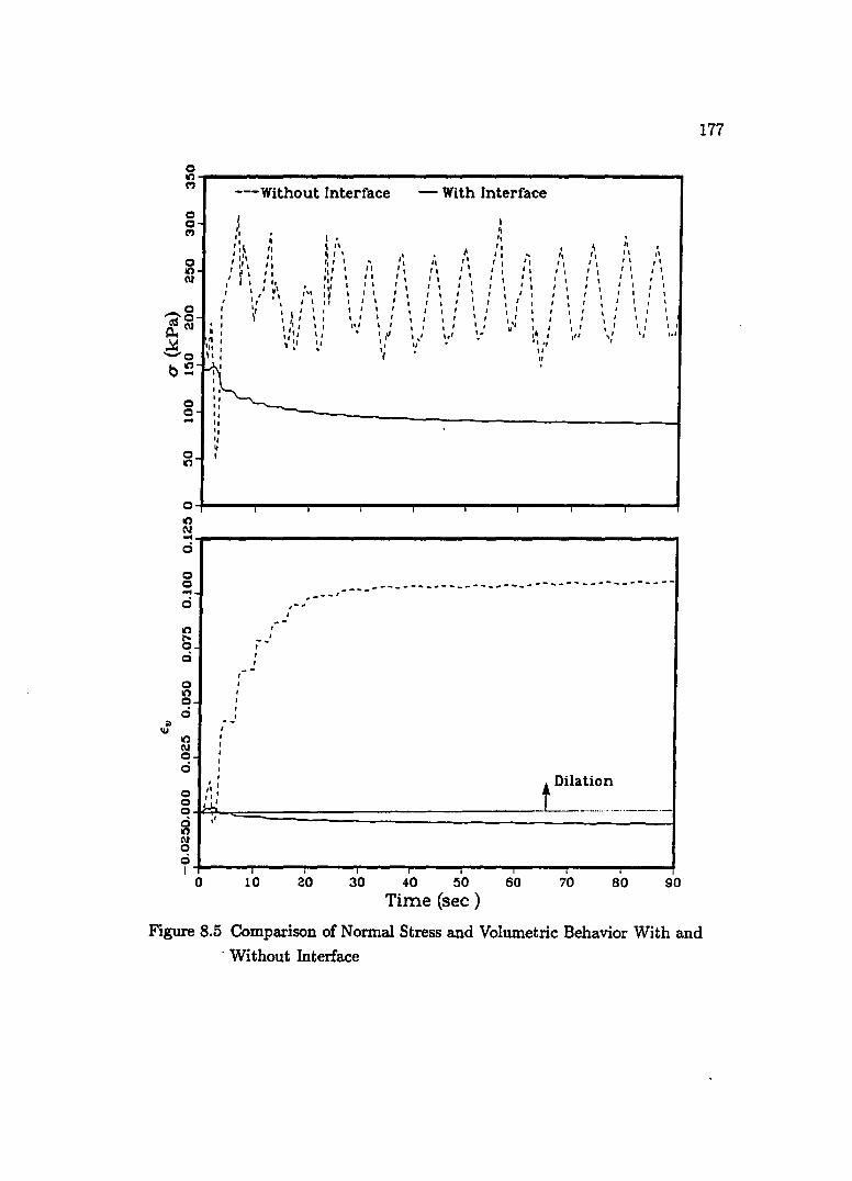
g~---------------------------------------------------, M
C) C) M
C) It) C\I
---Without Interface
I " ". , .
" :\" , " " , , , , :,~ ,: '.' ,
, I, I I ", I , I
"
'I , It 'I' I II I , ',I I ,
" ~, ''''1'1 ' ,
" " , ' , ,
- With Interface
It
" , , , , , ,
~
" , , , I
, ' ,
, ~
" " , ,
" '. I, 'I " I, , 'I
, " " , , ,
~
" ,
" " ' , ' , " , , , , , , , , , , , ,
I , , , , , , , ,
C) '2C) 1l.C\I
~, , ,\ r' ',:' I, ,,'"
, ",' " I' ~ : ~ ": ~ " ''',' "~ : .,,~,~,
, ~ ,"
" " " I I
" I,' , ,.
, " , : ',/'
, , "
, , , I , , , , , , , , , , I
,II \,' " ,.,
~ ,,' '1" -C)
~ " I "
b~
:> \U
C) :i~-~ ________________________________________________________________ --! C) " ... "
C) It)
" " ~ I
C)~----~--~~--~----~----~----~--~----~----~ It)
~~--------------------------------------------------~ d
C) C) ... d
1/'.1 l' C) c:i
C) It) C)
0
1/'.1 C\I C)
c:i
C) C) C)
g ell C)
c:i I
, . -'
, , ,',' ,,' ~
"
0
.--.---------------.---.- ----------------, ___ 1
,-. ,
i-,
t Dilation
10 20 30 40 50 so 70 80 90 Time (sec)
177
Figure 8.5 Comparison of Normal Stress and Volumetric Behavior With and . Without Interface

;0 III
It) N ~ Q
Q Q .-4
d
It) l'o Q d
Q It) Q d
It) N Q d
Q Q Q
S N Q
d I
With Iinterfa ~e
-
. -0.3 -0.2 -0.1 0.0 0.1 0.2
Shear Strain, "y
178
Without Inte face
• • 0.3 -0.3 -0.2 -0.1 0.0 0.1 0.2 0.3
Shear Strain, "y
Figure 8.6 Comparison of Volumetric Behavior vVith and 'Without Interface
179
this model. More over, this model is developed for dense sands thus exhibits
dilational behavior even during cyclic loading. This explains the failure of without
interface case to capture some of the essential ingredients of the cyclic behavior
such as cyclic compaction.
Figure (8.7) shows the vertical displacement along radial direction A - A
(Fig.8.3b) of the pile at various time intervals during the cyclic loading for with
(rough) and without interfaces. The Fig.(8.7) is enlarged and shown in Fig.(8.8).
These figures clearly show the concentration of vertical displacement (or relative
slip) within the interface zone for the case of with interface. Such localized effect
is not dominent in the case of without interface, where the vertical displacement
gradually damped out in radial direction. Hence, the localized shear effect in the
interface zone is very well captured by the with interface case.
Based on the comparison between with and without interface cases, it is
observed that the use of interface model is essential in order to properly model shear
transfer, volumetric behavior and localized relative slip (shear effect) in interface
zone.
8.2.4.2 Comparison of Pile Behavior: Rough and Smooth Interfaces
The effect of roughness of interface on the response of pile is demonstrated
in this section by comparing pile behavior with rough interface (Rn = 0.167 or
R = 0.902) and smooth interface (Rn = 0.057 or R = 0.309). Figures (8.9a) and
(8. 9b) show variation of shear stress with time (or number of loading cycle) and
hysteresis loop, respectively for rough and smooth interface cases. It is observed,
for the case of rough interface, the ultimate shear stress gradually decreases with
the increase of loading cycle and finally a steady state is reached approximately
after 11th cycle. In the case of smooth interface, however, the ultimate shear stress
virtually remains the same with the increase of loading cycle. Notice that the shear
stress for rough interface is always higher than that of smooth interface during the
entire loading cycle.

.. b~ ~o~----------____ ----------~ * ....
8: _0 ~.n C d)
E d)
ColO ~ . -0 Q, (J) ... o
o o
Time = 1.5 s
.--- ............................... . ,"'~ ......... .
.... ....
..... Without Interface - With Interface (Rough) --- With Interface (Smooth)
.... .. I +-----:-----:'---~--"'" b~ ~o,_------------------------~ * ....
8: _0
~.n C d)
E d)
Colo «I . -0 Q, (J) ... o -«10
Col • ... I/) ~I !:-.
~ o o
Time = 3.5 s
~ ............ . ' ... ~ ••••• I •••••••••••••••••••••••••••••
------------ -
Time = 2.5 s
...._---..-: ...... ..
.'
Time = 26.5 5
....................................... ....
180
i~--~--~----~----~, ~,------~---~---~----~ a 1 2 3
Radial Distance (m) 4- 0 123
Radial Distance (m)
Figure 8.7 Variation of Vertical Displacement of Line A-A (Fig.8.3) with
Radial Distance at Different Times During Cyclic Loading
4
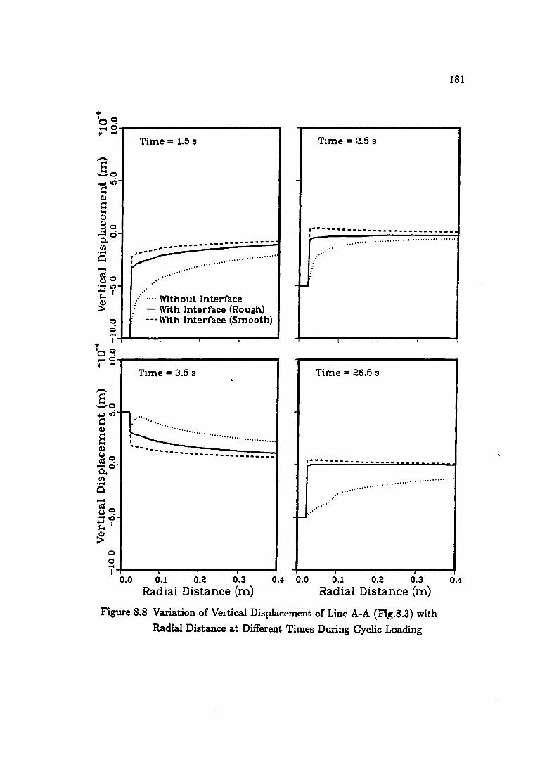
.. b~ ~o,-________________________ ~
* ....
'8 _0
~.ri ~ (I)
S (I) Q o «S • -0 c. (J) .-o -«So Q . .... .n t, ~
o Q
Time = 1.5 s
ttI"·, I
---.-.. --------.---.---~ ,." .... , .. , ............... ...........
.... ..... :: ... Without Interface j - With Interface (Rough) . ---With Interface (Smooth)
.. i~~--~----~----~----~ b~ ~o~ ______________________ ~
* ...
~ o
Time = 3.5 s
n.:·········· ...... . I~····"·""·" .. "· .. ·,,·· .. · .. · .. ·,, ..
--- .. _-----------------------
i~----~----~------~--~
181
Time = 2.5 s
.----._._--------------------I
......... .............................................. ....
Time = 26.5 5
.-----------------
~"
.. , .... ....
................................... .....
0.0 0.1 0.2 0.3 0.4 0.0 0.1 0.2 0.3 0.4
Radial Distance (m) Radial Distance (m)
Figure 8.8 Variation of Vertical Displacement of Line A-A (Fig.8.3) with
Radial Distance at Different Times During Cyclic Loading
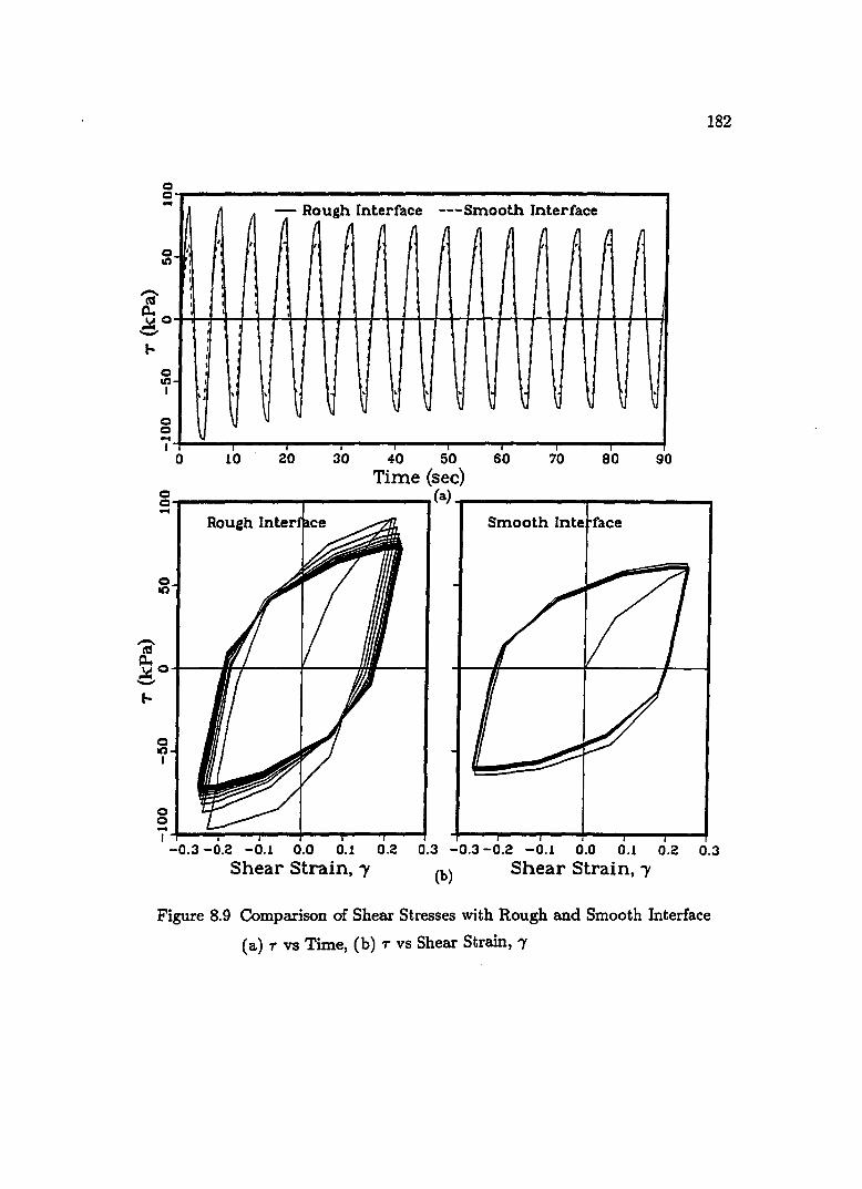
~
g~----------------------------------------------~ ~
o " 10
/ - Rough Interface ---Smooth Interface
t ~ ~ f (I t Iff I ". , , ~o ' ,
... o It)
I
\J \J \J .
\J \J \J \ o
7~-ij--~----~----~--~----~----~--~----~--~ o 10 20 30 40 50 60 70 80 90 Time (sec)
182
g~----------~----------~(~~----------~----------~ .... Smooth Inte face
"2 ~Q~----'~-------r------~'----~ ...
Q It)
I
Q o i~--~--~--~--~--~--~
-0.3 -0.2 -0.1 0.0 0.1 0.2 0.3 -0.3 -0.2 -0.1 0.0 0.1 0.2
Shear Strain, l' (b) Shear Strain, l' 0.3
Figure 8.9 Comparison of Shear Stresses with Rough and Smooth Interface
(a) T vs Time, (b) T vs Shear Strain, '1
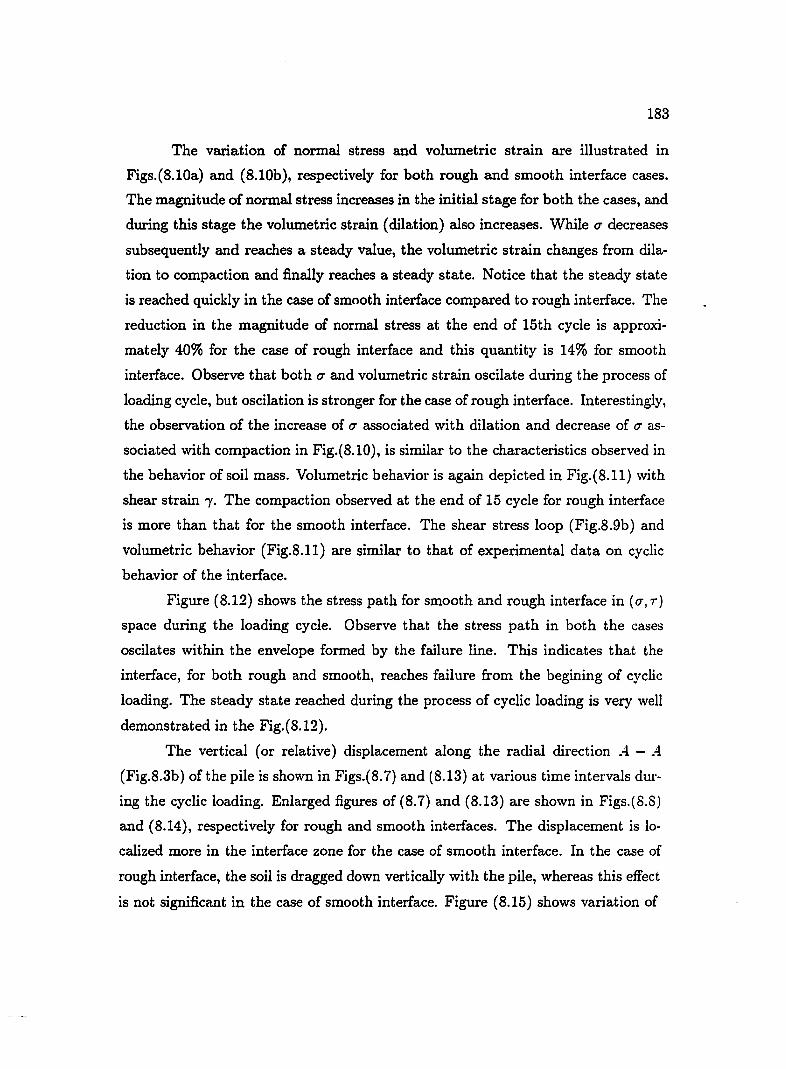
183
The variation of normal stress and volumetric strain are illustrated in
Figs.(8.lOa) and (8.lOb), respectively for both rough and smooth interface cases.
The magnitude of normal stress increases in the initial stage for both the cases, and
during this stage the volumetric strain (dilation) also increases. While 0' decreases
subsequently and reaches a steady value, the volumetric strain changes from clila
tion to compaction and finally reaches a steady state. Notice that the steady state
is reached quickly in the case of smooth interface compared to rough interface. The
reduction in the magnitude of normal stress at the end of 15th cycle is approxi
mately 40% for the case of rough interface and this quantity is 14% for smooth
interface. Observe that both 0' and volumetric strain oscilate during the process of
loading cycle, but oscilation is stronger for the case of rough interface. Interestingly,
the observation of the increase of (I associated with dilation and decrease of 0' as
sociated with compaction in Fig.(8.1O), is similar to the characteristics observed in
the behavior of soil mass. Volumetric behavior is again depicted in Fig.(8.11) with
shear strain;. The compaction observed at the end of 15 cycle for rough interface
is more than that for the smooth interface. The shear stress loop (Fig.8.9b) and
volumetric behavior (Fig.8.11) are similar to that of experimental data on cyclic
behavior of the interface.
Figure (8.12) shows the stress path for smooth and rough interface in ((I, r)
space during the loading cycle. Observe that the stress path in both the cases
oscilates within the envelope formed by the failure line. This indicates that the
interface, for both rough and smooth, reaches failure from the begining of cyclic
loading. The steady state reached during the process of cyclic loading is very well
demonstrated in the Fig.(8.12).
The vertical (or relative) displacement along the radial direction A. - A
(Fig.8.3b) of the pile is shown in Figs.(8.7) and (8.13) at various time intervals dur
ing the cyclic loading. Enlarged figures of (8.7) and (8.13) are shown in Figs.(8.8)
and (8.14), respectively for rough and smooth interfaces. The displacement is lo
calized more in the interface zone for the case of smooth interface. In the case of
rough interface, the soil is dragged down vertically with the pile, whereas this effect
is not significant in the case of smooth interface. Figure (8.15) shows variation of

0 10 ... 0 ~ ... 0 M ... 0
"2 N p.. ... .!:d -0
b::: 0 0 ... 0 0)
0 = t'l
100 .-t" * M
0 N
0 ... ~ 0
0 ... ;> I
1&1 0 N I
0 M I
0 ..;. I
0 an d, cQ I
, -
0 10
- Rough Interface - - - Smooth Interface
--, ..... ,---- ... -. "' .... - ...... - ..... - ... _-
20 30 40 50 Time (sec)
Dilation
I
so 70 80
184
, 90
Figure 8.10 Comparison of Normal Stress and Volumetric Behavior with Rough
and Smooth Interface
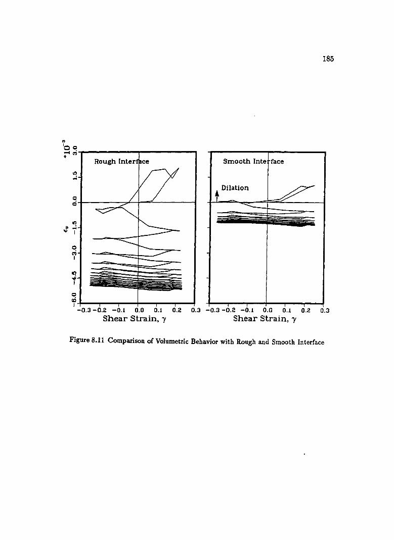
C'I
100
~ M~------------~-----------'
o o~--------~~+-~~------~
o M I
o
~~--~--~~--~--~---T--~
Smooth Inte face
-0.3 -0.2 -0.1 0.0 0.1 0.2 0.3 -0.3 -0.2 -0.1 0.0 0.1 0.2
Shear Strain, 'Y Shear Strain, 'Y
185
0.3
Figure 8.11 Comparison of Volumetric Behavior with Rough and Smooth Interface

0 0 ...
Failure 15
3 ------ --- 2 Roueh Interface
---0 IC)
'2 0.. ~o -...
0 IC)
I
".
0 0 ...
". ". ' .. '"
I
0 (a)
0 ... Smooth Interface
o F.i1Ure\ _-------------------~~ 3 2 __ ---
IC) __ ---------------
'2 ~o4----------------------------------
o IC)
I
o o
---- ----- - ... _---- ----- .. ---- .. ... .. -...
----
i~8~O------9~O------10~O------1~10------1~2-0------13~O------14TO------4150 a (kPa)
(b)
Figure 8.12 Cyclic Stress Path T VB (j
(a) Rough Interface, (b) Smooth Interface
186
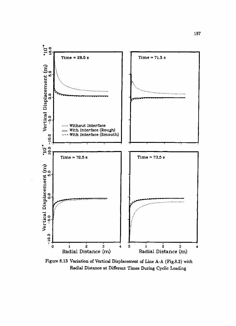
.. b~ ~o~------------------------~ * -I
E _0
~Iri ~ Q)
fa Q) Q o ~ . -0 c. (fl
;5
~o Q . .... .n tl ~
o o
Time = 28.5 s
......... "'"'0. ..........................
..... Without Interface - With Interface (Rough) --- With Interface (Smooth)
i~----~----~------~----~ .. b~ ~o,---~--------------------~ It -I
'8 _0
~Iri ~ Q)
fa Q) Q o ~ . -0 c. (fl
o ~o C,,) • .... .n tl ~
o o
Time = 72.5 s
...................................... ......
i~----~----~------~----~
Time = 71.5 s
.. '. ".
.. -. '" . ..... .................................
Time = 73.5 s
~ •••••• u •• " ......... .
I I
o 123
Radial Distance (m) 4- 0 1 2 3
Radial Distance (m)
Figure 8.13 Variation of Vertical Displacement of Line A-A (Fig.8.3) with
Radial Distance at Different Times During Cyclic Loading
187
4

.. 'o~ ~o~~-----------------------, * -4
E _0
-.l.n c: Q,)
S Q,) Q o ~ . -0 Q. rn ..... o ~o Q .
..... It) t, ~
o c::i
Time = 28.5 s ....... ". ......
". " . ......... , .... ....................
"'."
..... Without Interface - With Interface (Rough) --- With Interface (Smooth)
i~----~------~----~----~ .. 'o~ ~o~------------------------~ * -4
E _0
-.l.n c: Q,)
S Q,) Q o ~ . -0 Q.. rn . -o ~o Q .
• - It) t, ~
o c::i
Time = 72.5 s
.... ------- ................................ . . .,.- ...... . .... ...... ~ .....
..... .
Time = 71.5 s
." ..... .............. ..... "'0'
188
........... .................
.------------------------.. --
Time = 73.5 s
;.;. __ :,:. ___ :.::.: __ :.::.: __ :.:.; __ :.:.;--:.=..:--~--0=,,;;-- •
,---~
. .............. . . .... .... . .... . ...
i~----~----~~----~----~ , 0.0 0.1 0.2 0.3 0.4 0.0 0.1 0.2 0.3
Radial Distance (m) Radial Distance (m)
Figure 8.14 Variation of Vertical Displacement of Line A-A (Fig.8.3) with
Radial Distance at Different Times During Cyclic Loading
0.4

g~------------------------~ N
o _0 ca'" ~
6~ In In
f!o ~
rt:J ~:E cal <I.> ..co rt:J~
I o It) ... o o
Time = 1.5 s
' . ........ ....... I •••••••••••••••••••••••••••••
.... Without Interface - With Interface (Rough) - - - With Interface (Smooth)
~~-----T------~-----r----~
g~------------------------~ N
o It) ... o o
Time = 3.5 s
~ I'~~ ----------------
,.' .,.,
I.··· ...... .......... ....................
~4-----~------~----~~----~
Time = 2.5 s
~ :;.:. .. .
Ai ... ,· ............... "' ......... ..,WKh·Kh·b·HMHWHH
.. )
Time = 26.5 s
.. ~ \" : ",
1r-.. ~.:: ................................ . ' .. ~
0.0 0.1 0.2 0.3 0.4 0.0 0.1 0.2 0.3 Radial Distance (m) Radial Distance (m)
189
0.4
Figure 8.15 Variation of Shear Stress at Gauss Points (Located just above Line A-A,
Fig.8.3) with Radial Distance at Different Times During Cyclic Loading
190
shear stress on the gauss points, which lie just above line A - A (Fig.8.3b), along
radial direction. Here, acute variation of shear stress in the interface zone can be
observed clearly.
Apparently a decrease in shear stress (or softening behavior) is observed
during cyclic loading. This behavior is dominent for rough interface. The soften
ing shear behavior of interface is due to the normal stress-volumetric behavior of
interface. The cyclic volumetric compaction causes the interface normal stress to
decrease, which during failure state causes the shear stress to decrease. This ex
plains how normal stress-volumetric behavior of interface is coupled with the shear
stress transfer of pile-soil system.

191
CHAPTER 9
SUMMARY AND CONCLUSIONS
It has been identified in Chapter 1 that the nature and behavior of the
interface is an important phenomenon in the soil-structure interaction problems.
In order to obtain improved and reliable solution, use of proper interface model in
the solution method is essential. To this end, a constitutive model to describe the
essential features of the interface behavior is proposed. The model is implemented
in a finite element program to solve a boundary value problem. This chapter
summarizes the work described in" the previous chapters, and presents conclusions
based on the findings from this study.
9.1 Summary
(1) A constitutive model based on elasto plasticity theory is proposed (Chapter
4) herein to describe the behavior of the interfaces under static and cyclic
loading conditions. The proposed model considers associative, nonassocia
tive and strain-softening behavior in the hierarchical manner. The model
is a specialization of the generalized model developed for geologic (solid)
materials. A parameter called "interface roughness ratio, R" is defined in
order to model the interface behavior under different interface roughness.
Similarly, a cyclic parameter n is introduced to simulate the cyclic volu
metric behavior of the interfaces. Altogether ten parameters are required
to represent static loading. And an additional parameter (n) is required to
define cyclic behavior of the interfaces.
(2) Model parameters are determined (Chapter 5) using data from laboratory
test on the interfaces. Verification of the proposed model is performed by
comparing the model predictions with the experimental values of shear stress

192
ratio (T / (T) and volumetric behavior of sand-steel and sand-concrete inter
faces under various roughnesses, normal stresses and initial densities of sand.
Analysis of the model characteristics related to the volumetric and strain
softening behavior are presented. The model prediction at constant volume
condition and the effect of the displacement amplitude during cyclic loading
are discussed.
(3) A new algorithm for the drift correction is proposed (Chapter 6) and used
for the integration of elasto plastic constitutive relation of the interfaces to
perform back predictions. Performance of the algorithm is compared with
the existing algorithms. Using Lyapunov's Stability Theorem, it is proved
that the proposed algorithm is stable.
( 4) The proposed model for the interface is implemented in a nonlinear dynamic
finite element code to solve a boundary value problem involving dynamics
of an axially loaded pile (Chapter 8). The pile problem is solved for three
cases namely; (a) without interface, (b) with interface (or rough interface),
and (c) smooth interface.
9.2 Conclusions
(1) Comparison of model prediction (Chapter 5) with the data obtained from
experiments on the interface indicates that the proposed model performs
well. Predicted stress ratio (T / (T) compares well with the observed behav
ior, and the predicted volumetric behavior is satisfactory. The predicted
volumetric behavior shows general trend of the the observations such as
dominent dilational behavior of rough interfaces under monotonic loading,
and cyclic compaction. It is found that the proposed model can simulate
interface behavior under various roughnesses, normal stresses, initial densi
ties of sand, interface materials such as concrete, steel and types of sand,
and the effect of displacement amplitude during cyclic loading.
193
(2) Model parameters are related to various physical states during the inter
face deformation. The model prediction is found to be sensitive for the
parameters j.lP, j.lo, K., and n. (3) The proposed drift correction algorithm (Chapter 6) for constraint condition
is efficient and stable. Due to the generality, the algorithm can be applied
for any type of constitutive models. The performance of the algorithm is
yet to be seen in a hybrid formulation based finite element solution for a
boundary value problem.
(4) It is observed (Chapter 8) in the comparison between with and without
interface cases that the use of interface model is essential in order to properly
model shear transfer, volumetric behavior and localized relative slip in the
interface zone.
(5) The rough and smooth interface cases (Chapter 8) indicate degradation
of shear transfer from pile to soil, and volumetric compaction during the
progress of cyclic loading of the pile. The shear stress and volumetric com
paction reach a steady value during the process of cyclic loading. The stress
path of the interlace for rough and smooth interface shows that the interface
reaches failure from the begining of the cyclic loading. The degradation of
shear stress on the interface is due to the coupling effect of the normal stress
volumetric behavior with the shear behavior of the interface. In conventional
method, load capacity of the pile is calculated by using two quantities; ini
tial normal stress on the pile and skin friction coefficient. This method does
not provide information on the load-displacement behavior of piles. The
method presented here offers clear understanding of the load transfer mech
anism and gives improved solution procedure to compute load-displacement
behavior of piles over the conventional method.
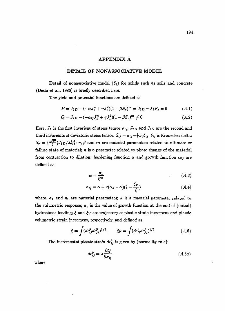
194
APPENDIX A
DETAIL OF NONASSOCIATIVE MODEL
Detail of nonMsociative model (81) for solids such as soils and concrete
(Desai et al., 1986) is briefly described here.
The yield and potential functions are defined as
F = J2 D - (-OlJf + 'YJl)(1 - {3Sr)m = hD - FbFs =0 (A.l)
Q- = J2D - (-OlQJf + 'YJl)(I- {3Sr)m =1= 0 (A.2)
Here, J I is the first invarient of stress tensor O'ij; J 2 D and JaD are the second and
third invarients of deviatoric stress tensor, Sij = O'ij-tJ18ij; 8ij is Kronecker delta;
Sr = (Yf)J3D/iiJJ; 'Y,{3 and m are material parameters related to ultimate or
failure state of material; n is a parameter related to phase change of the material
from coIrtraction to dilation; hardening function Ol and growth function OlQ are
defined as
(A.3)
(A.4)
where, al and 7]1 are material parameters; I'i, is a material parameter related to
the volumetric response; Olo is the value of growth function at the end of (initial)
hydrostatic loading; ~ and ev are trajectory of plastic strain increment and plastic
volumetric strain increment, respectively, and defined as
(A.5)
The incremental plastic strain defj is given by (normality rule):
8Q del!· = .A--
I) 80'ij (A.6a)
where

195
(A.6b)
and
(A.6c)
Here, dE,,, is the incremental strain. The incremental stress-strain relation is given
by
(A.7a)
where -fliLc 8F C
ep 8tTmn ijmn 8t1'"q pqkl C ijk1 = Cijkl -..2SL 8F
8tTr • Cturs 8t1'tu - H (A.7b)
Here, C:]'kl and Cijkl represent elastoplastic and elastic constitutive matrix of the
material, respectively. The Eq.(A.7a) can be used in the Eq.(7.3e) to formulate
stiffness matrix for elements representing soil.
196
LIST OF REFERENCES
Baker, R. and Desai, C.S., "Consequences of Deviatoric Normality in Plasticity
with Isotropic Strain Hardening," Int. J. Num. Analyt. Meth. in Geomech.,
Vol. 6, pp. 383-390, 1982.
Bathe, K.J., "Finite Element Procedures in Engineering Analysis," Prentice Hall,
Inc., New Jersey, 1984.
Boulon, M., "A Soil-Structure Incremental Interface Constitutive Equation Appli
cation to the Prediction of Piles Behavior," 2nd. Int. Conf. on Constitutive
Laws for Eng. Materials, Tucson, Arizona, Jan., 1987.
Brummund, W.F. and Leonards, G.A., "Experimental Study of Static and Dy
namic Friction Between Sand and Typical Construction Materials," ASTM,
J. Testing and Evaluation, Vol. 1, No.2, pp. 162-165, 1973.
Chen, Z. and Schreyer, H.L., "Simulation of Soil-Concrete Interfaces with Nonlocal
Constitutive Models," J. Eng. Meeh. ASCE, Vol. 113, No. 11, pp. 1665-
1667, 1987.
Desai, C.S., "A Consistent Finite Element Technique for Work-Softening Behav
ior," Proe. Int. Conf. on Compo Meth. in Nonlinear Meehs., (Oden, J.T.,
et al., eds.), Univ. of Texas, Austin, Texas, 1974.
Desai, C.S., "Numerical Design-Analysis of Piles in Sands," J. Geoteeh. Eng.
ASCE, Vol. 100, GT 6, pp. 613-625, 1974.
Desai, C.S., "A Dynamic Multi Degree-of-Freedom Shear Device," Report No. 8-
36, Dept. of Civil Eng., Virginia Tech., Blacksburg, VA, 1980.
Desai, C.S., "Behavior of Interfaces Between Structural and Geologic Media," A
State-of-the-Art paper, Int. Conf. Recent Advenees in Geoteeh. Earthq.
Eng. and Soil Dyn., St. Louis, MO, 1981.
o.
197
Desai, C.S., "A Nonlinear Dynamic Finite Element Code, SSTIN-DYN for the
Solution of Soil-Structure Interaction Problems", Private Communication,
1989.
Desai, C.S. and Abel, J.F., "Introduction to Finite Element Method," Van Nor
trand Reinhold Company, New York, 1972.
Desai, C.S., Drumm, E.C. and Zaman, M.M., "Cyclic Testing and Modeling of
Interfaces," J. Geotech. Eng. ASCE, Vol. 111, No.6, pp. 793-815, 1985.
Desai, C.S. and Fishman, K.L., "Constitutive Models for Rocks and Discontinuities
(Joints)," Rock Mechanics: 28th U.S. Symp., University of Arizona, Tucson,
AZ,1987.
Desai, C.S. and Fishman, !CL., "Plasticity Based Constitutive Model with As
sociated Testing for Joints," Int. J. Rock Mech. and Min. Sc., Under
Publication, 1988.
Desai, C.S. and Nagaraj, B.K., "Modeling for Cyclic Normal and Shear. Behavior
of Interfaces," J. Eng. Mech. ASCE, Vol. 114, No.7, pp. 1198-1217, 1988.
Desai, C.S. and Siriwardane, H.J., "Constitutive Laws for Engineering Materials,"
Prentice-Hall, Inc., New Jersey, 1984.
Desai, C.S., Somasundaram, S. and Frantziskonis, G., "A Hierarchical Approach
for Constitutive Modeling of Geologic Materials," Int. J. Num. Analyt.
Meth. in Geomech., Vol. 10, pp. 225-257, 1986.
Desai, C.S., Zaman, M.M., Lightner, G.J. and Sriwardane, H.J., "Thin-Layer Ele
ments for Interfaces and Joints," Int. J. Num. Analyt. Meth. in Geomech.,
Vol. 8, pp. 19-43, 1984.
Drumm, E.C., "Testing, Modeling and Application of Interface Behavior in Dy
namic Soil-Structure Interaction," Ph.D. Dissertation, University of Ari
zona, Tucson, Arizona, 1983.
198
Drumm, E.C. and Desai, C.S., "Detennination of Parameters for a Model for the
Cyclic Behavior of Interfaces," J. Earthq. Eng. and Struct. Dyn., Vol. 14,
pp. 1-18, 1986.
Eguchi, M., "Frictional Behavior Between Dense Sand and Steel Under Repeated
Loading," M.S. Thesis, Tokyo Institute of Technology, Japan, 1985. (in
Japanes).
Fishman, K.L., "Constitutive Modeling of Idealized Rock Joints Under Quasi
Static and Cyclic Loading," Ph.D. Dissertation, University of Arizona, Tuc
son, Arizona, 1988.
Fishman, K.L. and Desai, C.S., "A Constitutive Model for hardening Behavior of
Rock Joints," 2nd. Int. Con/. on Constitutive Laws for Eng. Materials,
Tucson, Arizona, Jan., 1987.
Frantziskonis, G. and Desai, C.S., "Elastoplastic Model with Damage for Strain
Softening Geomaterials," Acta Mechanica, Vol. 68, pp. 151-170, 1987.
Ghaboussi, J., Wilson, E.L. and Isenberg, J., "Finite Element for Rock Joint and
Interfaces," J. Soil Mech. and Found. Div., Vol. 99, No. SM 10, pp.
833-848, 1973
Goodman, R.E., Taylor, R.L. and Brekke, T.L., "A Model for the Mechanics of
Jointed Rock," J. Soil Mech. and Found. Div., Proc. of ASCE, Vol. 98,
No. SM 4, pp. 399-422, 1968.
Gopal, M., "Modern Control System Theory," Wiley Eastern ltd., 1984.
Griffiths, D.V. and Lane, P.A., "The Influence ofInterface Roughness on Problems
of Axisymmetric Soil/Structure Interaction," 2nd. Int. Con/. on Constitu
tive Laws for Eng. Materials, Tucson, Arizona, Jan., 1987.
Heuze, F.E. and Barbour, T.G., "New Models for Rock Joints and Interfaces," J.
Geotech. Eng. ASCE, Vol. 108, No.5, pp. 757-776, 1982.

199
Idriss, I.M., et al., "Analysis for Soil-Structure Interaction Effects for Nuclear Power
Plants," Report by the Ad Hoc Group in Soil-Structure Interaction, ASCE,
New York, 1979.
Isenberg, J. and Vaughan, D.K, "Nonlinear Effects in Soil-Structure Interaction,"
Proc. Symp. on Implementation of Compo Procedures and Stress-Strain
Laws in Geotech. Eng., Chicago. pp. 29-44, 1981.
Ishihara, K and Towhata, I., "Dynamic Response Analysis of Level Ground Based
on the Effective Stress Method," Soil Mechanics-Transient and Cyclic Loads,
Pande, G.N. and Zienkiewics, O.C. (edt.), John Wiley & Sons, pp. 133-172,
1982.
Jardine, R.J. and Potts, D.M., "Hutton Tension Leg Platform Foundations: Pre
diction of Driven Pile Behavior," Geotechnique, Vol. 38, No.2, pp. 231-252,
1988.
Kane, W.F. and Drumm, E.C., "A Modified 'Cap' Model for Rock Joints," Rock
Mechanics: £8th U.S. Symp., University of Arizona, Tucson, AZ, 1987.
Kishida, H. and Uesugi, M., "Tests of the Interface Between Sand and Steel in the
Simple Shear Apparatus," Geotechnique, Vol. 37, No. 12, pp. 45-52, 1987.
Kulhawy, F.H. and Peterson, M.S., "Behavior of Sand-Concrete Interfaces," Proc.
6th Pan American Congo on Soil Mech. and Found. Eng., Vol. 2, pp.
225-236, 1979.
Matsuoka, H. and Sakakibara, K, "A Constitutive Model for Sands and Clays
Evaluating Principal Stress Rotation," Soils and Foundations, Vol. 27, No.
4, pp. 73-88, 1987.
Mroz, Z. and Norris, V.A., "Elastoplastic and Viscoplastic Constitutive Models
for Soils with Application to Cyclic Loading," Soil Mechanics-Transient and
Cyclic Loads, Pande, G.N. and Zienkiewics, O.C. (edt.), John Wiley & Sons,
pp. 173-217, 1982.

.200
Nagaraj, B.K., "Modeling of Normal and Shear Behavior of Interfaces in Dynamic
Soil-Structure Interaction," Ph.D. Dissertation, University of Arizona, Tuc
son, Arizona, 1986.
N avayogarajah, N., "Modeling of Initial Density and Normal Stress Effect on Direct
Shear Behavior of Sand," Report, Dept. of Civil Eng. & Eng. Mechanics,
University of Arizona, Tucson, Arizona, 1988.
Navayogarajah, N., "An Algorithm for Drift Correction Method: Application to
Interface Problems," Report, Dept. of Civil Eng. & Eng. Mechanics, Uni
versity of Arizona, Tucson, Arizona, 1988.
Ogata, K., "Discrete-Time Control Systems," Prentice Hall, Inc., New Jersey, 1987.
Ortiz, M. and Popov, E.P., "Accuracy and Stability of Integration Algorithms for
Elastoplastic Constitutive Relations," Int. J. Num. Meth. in Eng., Vol. 21,
pp. 1561-1576, 1985.
Ortiz, M. and Simo, J.C., "An Analysis of a New Class of Integration Algorithms
for Elastoplastic Constitutive Relations," Int. J. Num. Meth. in Eng., Vol.
23, pp. 353-366, 1986.
Owen, D.R. and Hinton, E., "Finite Elements in Plasticity: Theory and Practics,"
Pineridge Press Ltd., Swansea, U.K., 1980.
Pande, G.N. and Sharma, K.G., "On Joint/Interface Elements and Associated
Problems of Numerical Illconditioning," Short Communications, Int. J.
Num. Analyt. Meth. in Geomech., Vol. 3, No.3, 1979.
Plesha, M.E., "Constitutive Models for Rock Discontinuities with Dilata.ncy and
Surface Degradation," Int. J. Num. Analyt. Meth. in Geomech., Vol. 11,
pp. 345-362, 1987.
Potts, D.M. and Genes, A., "A Critical Assement of Methods of Correcting for
Drift from the Surface in Elasto-Plastic Finite Element Analysis," Int. J.
Num. Analyt. Meth. in Geomech., Vol. 9, pp. 149-159, 1985.
201
Potyondy, J.G., "Skin Friction Between Various Soils and Construction Materials,"
Geotechnique, Vol. 11, No.4, pp. 339-353, 1961.
Selvadurai, A.P.S. and Faruque, O.M., "The Influence of Interface Friction on the
Performance of Cable Jacking Tests of Rock Masses," Proc. Symp. on
Implementation of Compo Procedures and Stress-Strain Laws in Geotech.
Eng., Chicago, pp. 169-184, 1981.
Sharma, K.G. and Desai, C.S., "Analysis and Implementation of Thin-Layer Ele
ment for Interfaces and Joints," Submitted to J. Eng. Mech. ASCE, 1990.
Somasundram, S. and Desai, C.S., "Modeling and Testing for Anisotropic Behavior
of Soils," J. Eng. Mech. ASCE, Vol. 114, No.9, pp. 1473-1496, 1988.
Toki, K, Sato, T. and Miura, F., "Separation and Sliding Between Soil and Struc
ture During Strong Ground Motion," Earthquake Eng. and Stru. Dyna.,
Vol. 9, pp. 263-277, 1981.
The Earth Technology Corporation (ERTEC), "Pile Segment Tests-Sabine Pass,
Some Aspects of the Fundamental Behavior of Axially Loaded Piles in Clay
Soils," ETC Report No. 85-007, Dec. 1986.
Uesugi, M., "Friction Between Dry Sand and Construction Materials," Ph.D. Dis
sertation, Tokyo Institute of Technology, Japan, 1987.
Uesugi, M. and Kishida, H., "Influential Factors of Friction Between Steel and Dry
Sands," Soils and Foundations, Vol. 26, No.2, pp. 33-46, 1986.
Uesugi, M. and Kishida, H., "Frictional Resistance at Yielding Between Dry Sand
and Mild Steel," Soi13 and Foundations, Vol. 26, No.4, pp. 139-149, 1986.
Uesugi, M., Kishida, H. and Tsubakihara, Y., "Behavior of Sand Particles in Sand
Steel Friction," Soils and Foundations, Vol. 28, No.1, pp. 107-118, 1988.
Wolf, J.P., "Dynamic Soil-Structure Interaction," Pretice-Hall, Inc., Englewood
Cliffs, N.J., 1985.

202
Yoshimi, Y. and Kishida, T., "Friction Between Sand and Metal Surface," Proc.
10th Int. ConI. SMFE, Vol. 1, pp. 831-834, 1980.
Yoshimi, Y. and Kishida, T., "A ring Torsion Apparatus for Evaluating Friction
Between Soil and Metal Surfaces," Geotechnical Testing J., Vol. 4, No.4,
Dec., pp. 145-152, 1981.
Zaman, M.M., "Influence of Interface Behavior in Dynamic Soil-Structure Interac
tion Problems," Ph.D. Dissertation, University of Arizona, Tucson, Arizona,
1982.
Zaman, M.M., Desai, C.S. and Drumm, E.C., "Interface Model for Dynamic SQil
Structure Interaction," J. Geotech. Eng. ASCE, Vol. 110, No.9, pp.
1257-1273, 1984.
Zeinkiewicz, O.C., Best, B., Dullage, C. and Stagg, K.G., "Analysis of Nonlinear
Problems in Rock Mechanics with Particular Reference to Jointed Rock
Systems," Proc. 2nd. Congo on the Int. Soc. lor Rock Mech., Belgrad, Vol.
3, pp. 501-509.
Zienkiewicz, O.C., Leung, K.H. and Pastor, M., "Simple Model for Transient Soil
Loading in Earthquake Analysis. I. Basic Model and Its Application," Int.
J. Num. Analyt. Meth. in Geomech., Vol. 9, pp. 453-476, 1985.
Zubelewicz, A., O'Connor, A., Dowding, C.H., Belytschko, T. and Plesha, M., "A
Constitutive Model for the Cyclic Behavior of Dilatant Rock Joints," 2nd.
Int. ConI. on Constitutive Laws lor Eng. Materials, Tucson, Arizona, .Jan.,
1987.
Related Documents