Supplementary materials SM2.1 (Drivers) | IPBES

Supplementary materials SM2.1 (Drivers)

Contents

1. Additional figures ................................................................................................................................... 3

2. Additional text ....................................................................................................................................... 43

2.1. Maintain nature or meet society’s many short-run goals? (SECTION 2.1.2.1) ..................... 43

2.2. Inequalities (SECTION 2.1.2.2) ................................................................................................. 43

2.3. Fisheries, and aquaculture and mariculture (SECTION 2.1.11.1) .......................................... 44

2.4. Agriculture & Grazing (crops, livestock, agroforestry) (SECTION 2.1.11.2) ....................... 45

2.5. Forestry (logging for wood & biofuels) (SECTION 2.1.11.3) .................................................. 45

2.6. Mining: minerals, metals, oils and fossil fuels (SECTION 2.1.11.5) ....................................... 46

2.7. Infrastructure (dams, cities, roads) Urbanization and infrastructure (SECTION 2.1.11.6) 47

2.8. Illegal activities with direct impacts on nature (SECTION 2.1.11.10) .................................... 47

2.9. Evolving economic & Environmental tradeoffs (SECTION 2.1.18.2) .................................... 48

3. Selected recent critical references included in this report beyond the May 2018 threshold .......... 54

4. Methods for literature review .............................................................................................................. 55

4.1. Key messages, outline and iterative literature review steps ..................................................... 55

4.2. Global policy relevant issues....................................................................................................... 55

4.3. In-depth analysis of the different subsections ........................................................................... 55

4.4. Global overview ........................................................................................................................... 55

4.5. Systematic assessment of the amount of literature available on interactions between indirect

drivers, actions and direct drivers ............................................................................................................ 56

5. Data acquisition ..................................................................................................................................... 61

5.1. Core and highlighted IPBES indicators .................................................................................... 61

5.2. Publicly available data ................................................................................................................ 61

5.3. Data bases contributed by contributing authors ...................................................................... 61

6. Data analysis .......................................................................................................................................... 61

6.1. Trends ........................................................................................................................................... 61

6.2. Maps ............................................................................................................................................. 62

6.2.1. Static .................................................................................................................................... 62

6.2.2. Trends .................................................................................................................................. 62

6.3. Meta-analysis ............................................................................................................................... 63

6.4. Synthesis pathways ...................................................................................................................... 63

7. Data sources........................................................................................................................................... 64

List of figures

- S1: Global temporal trends in indirect drivers

- S2: income levels and IPBES regions

- S3: Temporal trends in indirect drivers for IPBES regions

- S4: Different views of well-being and current conditions

- S5: Trends in inequality among and within countries

- S6: Contrasting lifestyles

- S7: Footprint, biocapacity and water footprint

- S8: Agricultural share of total credit

- S9: Agriculture intensification by continent

- S10: Antibiotic use and resistance worldwide

- S11: Flows of natural resources embedded into trade

- S12: Water and land embedded into trade

- S13: Types of protected areas and temporal trends.

- S14: Trends in conservation policies for countries with different income levels.

- S15: Temporal patterns of payments for ecosystem services

- S16: Temporal trends for participation of countries with different income levels into

global agreements

- S17: Global temporal trends for selected indicators of actions and direct drivers

- S18: Temporal trends for selected indicators of actions and direct drivers per IPBES

region

- S19: Impacts of fisheries and aquaculture

- S20: Global trends in livestock density

- S21: Temporal trends in selected indicators of agriculture 1960-2015 for countries

with different income level

- S22: Temporal trends in wood and biofuel extraction

- S23: Temporal trends in selected indicators of relocations of goods and people

- S24: Land use changes 1992-2015

- S25: Temporal trends in material extraction

- S26: Spatial patterns of temporal trends in biomass extraction

- S27: Temporal trends in selected indicators of pollution

- S28: Spatial patterns of temporal trends in pollution

- S29: Trends in alien species per IPBES region

- S30: Preliminary metanalysis of differences in rates of change in selected indicators

for countries using World Bank income categories.

- S31: Battle deaths

- S32: Water scarcity and food riots.

- S33: Economic growth requires security

- S34: Regime shifts documented to date across the planet

- S35: Eutrophication, regime shifts in coastal systems, documented for one

developed countries

1. Additional figures

Figure S1. Global temporal trends for selected indicators of indirect drivers.

The data shown are global trends, per country, with a shadow representing 95% confidence

intervals unless otherwise stated. A) Child mortality rate: Mortality rate, under-5 (per 1,000

live births), B) Human Development Index: is a summary measure of average achievement

in key dimensions of human development: a long and healthy life, being knowledgeable

and have a decent standard of living. C) Calorie intake: Kilocalories consumed per person

per day, D) Gross Domestic product: GDP per capita is gross domestic product divided by

midyear population, Data are in current U.S. dollars., E) Globalization index: The KOF

Globalization Index measures the economic, social and political dimensions of

globalization., F) Domestic material consumption per capita: all materials used by the

economy, either extracted from the domestic territory or imported from other countries, per

capita, G) Merchandise exports: value of goods provided to the rest of the world per

country valued in current U.S. dollars., H) Total population: Number of people, I)

Proportion of urban population: Proportion of the total population that is urban, which

refers to people living in urban areas, J) International Migrant Stock: International migrant

stock is the number of people born in a country other than that in which they live (includes

refugees), K) Absence of conflict as an indicator of political stability: Index that measures

perceptions of the likelihood that the government will be destabilized or overthrown by

unconstitutional or violent means, including politically-motivated violence as well as

terrorism, L) Protection of key biodiversity areas: measures progress towards protecting the

most important sites for biodiversity in % of such sites per country. (AZEs). Values

provided are averages of country values for World Bank income categories (unless stated

otherwise).

Sources: BirdLife International, 2018; KOF Swiss Economic Institute, 2018; Land Portal,

2018; Roser & Ritchie, 2017a; UNDP, 2017; World Bank, 2018n, 2018t, 2018e, 2018s,

2018g, 2018k; WU & Dittrich, 2014).

Figure S2. Countries have been divided into different income levels by the World Bank.

Inequities among countries are increasing through time. a) Trend of Gross domestic product

(GDP) per capita, current (1,000 U$) from 1960 to 2015; the values shown are average

values among countries within different income level categories, using World Bank income

categories. b) Map of IPBES regions and income levels; the colors in the map represent a

combination of incomes and geographic regions; for instance, blue represents Asia-Pacific,

while different intensities of blue represent different income levels. Source: (World Bank,

2018e).

Figure S3. Temporal trends in selected indicators of indirect drivers for the four IPBES

regions. The data shown are trends, per country, averaged for each of IPBES regions.

Panels shown are: A) Child mortality rate: Mortality rate, under-5 (per 1,000 live births), B)

Human Development Index: is a summary measure of average achievement in key

dimensions of human development: a long and healthy life, being knowledgeable and have

a decent standard of living. C) Calorie intake: Kilocalories consumed per person per day,

D) Gross Domestic product: GDP per capita is gross domestic product divided by midyear

population, Data are in current U.S. dollars., E) Globalization index: The KOF

Globalization Index measures the economic, social and political dimensions of

globalization., F) Domestic material consumption per capita: all materials used by the

economy, either extracted from the domestic territory or imported from other countries, per

capita, G) Merchandise exports: value of goods provided to the rest of the world per

country valued in current U.S. dollars., H) Total population: Number of people, I)

Proportion of urban population: Proportion of the total population that is urban, which

refers to people living in urban areas, J) International Migrant Stock: International migrant

stock is the number of people born in a country other than that in which they live (includes

refugees), K) Absence of conflict as an indicator of political stability: Index that measures

perceptions of the likelihood that the government will be destabilized or overthrown by

unconstitutional or violent means, including politically-motivated violence as well as

terrorism, L) Protection of key biodiversity areas: measures progress towards protecting the

most important sites for biodiversity in % of such sites per country. (AZEs). Values

provided are averages of country values for World Bank income categories (unless stated

otherwise).

Sources: BirdLife International, 2018; KOF Swiss Economic Institute, 2018; Land Portal,

2018; Roser & Ritchie, 2017a; UNDP, 2017; World Bank, 2018e, 2018t, 2018s, 2018g,

2018k, 2018n; WU & Dittrich, 2014.

Figure S4. Diversity of well-being indicators current conditions in different countries for

those indicators. a) The different views of well-being include very different dimensions. b)

The diversity of dimensions of well-being is reflected in the variety of well-being indicators

and indices. c) Countries differ in their current conditions with respect to well-being along

two independent axes: one heavily influenced by income and societal conditions, and

another one strongly influenced by biodiversity conditions; each dot is a country, the

position in the graph is based on data for all indicators and principal component analysis.

Source: Breslow et al., 2014; EPI, 2018; HPI, 2016; McGregor et al., 2015; UN, 2016a;

UNU-IHDP & UNEP, 2014; WHI, 2017.

Figure S5. Trends in inequality among and within countries. a) Global trends in within and

among country inequality (1820~1992). b) Inequality measured using the Gini coefficient

for 2013 for different countries; The Gini coefficient is based on the comparison of

cumulative proportions of the population against cumulative proportions of income they

receive, and it ranges between 0 in the case of perfect equality and 100 in the case of

perfect inequality. c) Trends of changes in the Gini coefficient between 1981 and 2014,

based on the average values per country using world bank income categories; the temporal

data is analyzed using a linear regression to identify those with significant increase

(positive) or decrease (negative). d) Palma Ratio. Sources: Bourguignon & Morrisson,

2002; Fisher, 2013; World Bank, 2005, 2018f, 2018p)

Figure S6. Contrasting lifestyles and new demands from nature 1960-2010. a) Energy use:

Average energy use in tons of oil equivalent per capita, b) Total Mobile cellular

subscriptions (1,000 per 100 people). c) Prevalence of obesity in the adult population (18

years and older) (% of the total population). d) Prevalence of severe food insecurity in the

total population (2014-16) as % of the total population in countries affected. E) Protein

Consumption Exceeds Average Estimated Daily Requirements in All the World’s Regions,

and is Highest in Developed Countries g/capita/day in 2009.

Average values are calculated for countries within World Bank income categories. Data

sources: (FAO, 2018f; Ranganathan et al., 2016; Roser & Ritchie, 2017b; World Bank,

2018d, 2018m)

f

Figure S7. Trends in ecological footprint, biocapacity (capacity to supply renewable

resources and absorb waste) and water footprint: Trend of a) total values, and b) per capita

values of ecological footprint and biocapacity (1961~2012), and c) Trend of Average

values of Water Footprint (1996~2013). Average values per country using world bank

income categories. The Ecological Footprint includes all the cropland, grazing land, forest

and fishing grounds required to produce the food, fiber and timber it consumes, to house its

infrastructure and to absorb its waste (currently limited to CO2 from fossil fuel combustion,

cement production, anthropogenic forest fires and bunker fuels). The biocapacity refers to

the capacity of ecosystems to regenerate what people demand from those surfaces i.e. to

produce biological materials used by people and to absorb waste material generated by

humans, under current management schemes and extraction technologies.

The water footprint includes green water, blue waterand grey footprint. Ecological footprint

and biocapacity are expressed in global hectares; water footprint is expressed in Millions of

M3/year. Data shown are country data averaged per World Bank Income category.

Source: IPBES Technical Support Unit on Knowledge and Data (Borucke et al., 2013;

Galli, et al., 2014; Hoekstra & Mekonnen, 2012).

Figure S8. Agriculture Share of Total Credit by region and the world, since 1991 to 2016

(LAC = Latin America and the Caribbean). Source: (FAO, 2018a)

Figure S9. Agriculture intensification by continent, assessing the relationship between

yield and amount of land for the case of cereals. Source: (World Bank, 2018b, 2018j)

Cerealyield(kg/ha)(ha)(1961=100)

Landundercereal(ha)(1961=100)

2.1.2

y=-1.7492x+318.1R²=0.27705

100

150

200

250

300

40 60 80 100 120

LatinAmerica&Caribbean-highincome

y=13.991e0.0185x

R²=0.40499

100

200

300

400

100 120 140 160

LatinAmerica&Caribbean- middle

income

y=0.8418x+33.654R²=0.39001

100

120

140

160

180

100 120 140 160

EastAsia&Pacific-highincome

y=1.4478xR²=0.25639100

150

200

250

100 120 140

EastAsia&Pacific-middleincome

y=1.9493e0.0386x

R²=0.34258

100

150

200

250

300

100 110 120

SouthAsia- middleincome

y=81.375ln(x)- 268.64R²=0.87029100

120

140

160

180

100 150 200 250

Sub-SaharanAfrica- lowincome

y=0.9294xR²=0.40828

100

120

140

160

180

200

220

100.00150.00200.00250.00

Sub-SaharanAfrica-middleincome

Figure S10. Antibiotic use worldwide (2015). The Center for Disease Dynamics,

Economics and Policy (CDDEP), a non-profit group headquartered in Washington DC,

based the analysis on data from scientific literature and national and regional surveillance

systems. The organization used this to calculate and map the rate of antibiotic resistance for

12 types of bacteria in 39 countries, and trends in antibiotic use in 69 countries over the

past 10 years or longer. Sources: (Reardon, 2015); https://resistancemap.cddep.org

Figure S11. Flows of natural resources embedded into trade. a) Displacements of forest

area and embodied in trade of wood products, and of agricultural area embedded in

agricultural products, b) Main material flows between the forestry and agricultural sectors

of Costa Rica, and the international market, resulting from the use of wood pallets to export

the five main agricultural products exported on wood pallets over the past three decades

(bananas, pineapples, melons, palm oil and cassava). The color of arrows represents the

nature of the corresponding flows, while their width has been adapted to the relative size of

the flows for the years 1998 and 2013. Flows of pallets are expressed in number of items

(blue), flows of wood in RWE cubic meters (green), and flows of agricultural products (on

pallets or not) in tons (orange). Numbers in grey refer the three questions addressed in this

chapter. Source: Jadin, et al., 2016a; 2016b.

Figure S12. Water and land embedded into trade. A) A global map of the land-grabbing

network: land-grabbed countries (green disks) are connected to their grabbers (red

triangles) by a network. Based in data on table S1 but considering only 24 major grabbed

countries (as in Table 1). Relations between grabbing (red triangles) and grabbed (green

circles) countries are shown (green lines) only when they are associated with a land

grabbing exceeding 100,000 ha, b) Water grabbing in the 24 most land-grabbed countries.

Green and maximum blue water grabbing. Source: (Rulli et al., 2013)

Figure S13. a) Types of governance of Protected Areas and temporal trends in amount of

protected area by category. Source: own elaboration based on IUCN data.

b) Total extent, by area, of terrestrial and marine protected areas in the WDPA in each of

the six IUCN Management Categories between 1950-2014. There are some overlaps

between different IUCN Management Categories, hence total area does not equal global

protected area. Source: Borrini-Feyerabend & Hill, 2015; Dudley, 2008; Juffe-Bignoli et

al., 2014.

Figure S14. Temporal trends in protection policies for countries with different income

levels. Data shown are average values per country using world bank income categories.

(using World Bank typology). a) Percentage of protected area coverage in marine and

terrestrial regions in 2017. The protected areas were calculated using the April 2016 version

of the WDPA (World Database on Protected Areas), b) Percentage of protected area

management effectiveness in 2015. c) Total protected areas in 2015 (km2). d) Protected

areas assessed on management effectiveness in 2015 (km2). d) Protected areas assessed on

management effectiveness in 2015 (%). Source: Coad et al., 2015; UNEP-WCMC &

IUCN, 2016; www.protectedplanet.net

ProtectedArea(km2)2015

Global HighI-OECD HighI-Oil

OtherHigh-I UpperMiddle-I LowerMiddle-I

Low-I

PAAssessed on ManagementEffectiveness (km2)2015

Global

HighI-OECD

HighI-Oil

OtherHigh-I

UpperMiddle-I

PAAssessed on ManagementEffectiveness (%)2015

Global

HighI-OECD

HighI-Oil

OtherHigh-I

UpperMiddle-I

0

10

20

30

40

50

Global

1− High

Incom

e OECD

3− Othe

r high

incom

e

4− Upp

er midd

le inco

me

5− Lo

wer midd

le inco

me

6− Lo

w incom

e

% o

f Pro

tecte

d A

rea A

ssessed

[Not area−corrected]

Protected Area Management Effectiveness in 2015

*Visuals prepared by the IPBES Knowledge and Data TSU based on raw data provided by indicator holders.

a

b

cd e

Figure S15. Temporal patterns of payments for ecosystem services. a) Compliance

Biodiversity offsets and regulation; b) Compliance forest carbon. Source: Salzman et al.,

2018.

Figure S16. Temporal trends for participation of countries with different income levels into

global agreements. Data shown are number of participating countries per year per World

Bank Income level category. a) United Nation Framework Convention on Climate Change

from 1992 to 2015, b) Convention of fishing and conservation of the living resources of the

high seas from 1958 to 2012, c) Montreal Protocol from 1988 to 2012, d) Convention on

Biological Diversity from 1992 to 2015, e) Convention of the Conservation of Antarctic

0

10

20

30

40

50

60

1992 1995 1998 2001 2004 2007 2010

NumberCountryParties

Year

UnitedNationsFrameworkConvention

onClimateChange

0

5

10

15

20

1958 1968 1978 1988 1998 2008Numberofparticipatingcountries

Dataof entry

Conventionoffishingandconservationof

thelivingresourcesofthehighseas

0

10

20

30

40

50

60

1988 1991 1994 1997 2000 2003 2006Num

ber

ofparticipatingcountries

Dataof entry

MontrealProtocol

0

10

20

30

40

50

60

1992 1995 1998 2001 2004 2007 2010 2013

Num

ber

ofparticipatingcountries

Year

ConventiononBiologicalDiversity

0

5

10

15

20

1961 1971 1981 1991 2001 2011

Numberofparticipatingcountries

Year

ConventionontheConservationofAntarcticMarineLivingResources

0

5

10

15

20

25

30

35

2011 2012 2013 2014 2015 2016 2017 2018

Countriesparties

Year

NagoyaProtocol

a b

c d

e f

Marine Living Resources from 1961 to 2017 and f) Nagoya Protocol from 2011 to 2017.

Average values using world bank income categories Sources: Australian Government -

Department of the Environment and Energy, 2017; CBD, 2018a, 2018b; UN - Secretariat to

the Antartic Treaty, 2018; UN, 1966; United Nations, 2018

Figure S17. Global temporal trends for selected indicators of actions and direct drivers.

Data shown are country averages with a shadow representing 95% confidence intervals

unless otherwise stated. A) Fertilizer use: Fertilizer consumption measures the quantity of

plant nutrients (kg) used per unit of arable land per year; B) Fraction of cultivated and

urban area: Proportion of total area of country with cultivated and urban land cover, based

on ESA CCI Global Land Cover v2.0.7; C) Extraction of living biomass: Millions of tons

per year extracted from agriculture, forestry, fishing, hunting and other types of living

biomass; D) Extraction of non-living materials: Millions of tons per year extracted of fossil

fuels, metal ores, and minerals for construction and industry; E) Per capita greenhouse

gases emissions: metric tons of CO2 emitted per year; F) Air Pollution: mean annual

exposure to particles larger than 2.5 micrometer of diameter in micrograms per cubic meter;

G) Alien species: Cumulative number of first records of alien species; H) Temperature

anomalies: measured as the temperature in a given year minus that of the reference period

(1960-1969) in degrees celsius - In this case the confidence interval is provided by the

modelling tool. I) Biodiversity intactness index: relative change in abundance of native

species as compared to a pristine system- values are country averages weighted by country

Net Primary Productivity. Source: ESA CCI, 2017; FAO, 2018b; Jones et al., 2012;

Newbold et al., 2016; OECD, 2018b; Seebens et al., 2017; World Bank, 2018r; WU &

Dittrich, 2014.

Figure S18. Global temporal trends for selected indicators of actions and direct drivers per

IPBES region. Data shown are country averages per IPBES region. A) Fertilizer use:

Fertilizer consumption measures the quantity of plant nutrients (kg) used per unit of arable

land per year; B) Fraction of cultivated and urban area: Proportion of total area of country

with cultivated and urban land cover, based on ESA CCI Global Land Cover v2.0.7; C)

Extraction of living biomass: Millions of tons per year extracted from agriculture, forestry,

fishing, hunting and other types of living biomass; D) Extraction of non-living materials:

Millions of tons per year extracted of fossil fuels, metal ores, and minerals for construction

and industry; E) Per capita greenhouse gases emissions: metric tons of CO2 emitted per

year; F) Air Pollution: mean annual exposure to particles larger than 2.5 micrometer of

diameter in micrograms per cubic meter; G) Alien species: Cumulative number of first

records of alien species; H) Biodiversity intactness index: relative change in abundance of

native species as compared to a pristine system- values are country averages weighted by

country Net Primary Productivity. Source: ESA CCI, 2017; FAO, 2018b; Newbold et al.,

2016; OECD, 2018b; Seebens et al., 2017; World Bank, 2018r; WU & Dittrich, 2014.

Figure S19. Impacts of fisheries and aquaculture. a) Absolute difference in 2013 versus

2008 per-pixel stressor intensities for four representative stressors. a.1) Sea surface

temperature anomalies, b.1) nutrient input, c.1) demersal destructive fishing, and d.1)

pelagic high bycatch fishing. Positive scores represent an increase in stressor intensity.

Note that color scales differ among panels and are nonlinear, b) Ecological links between

intensive fish and shrimp aquaculture and capture fisheries. Thick blue lines refer to main

flows from aquatic production base through fisheries and aquaculture to human

consumption of seafood. Numbers refer to 1997 data and are in units of megatons (million

metric tons) of fish, shellfish and seaweeds. Thin blue lines refer to other inputs needed for

production. Hatched red lines indicate negative feedbacks. Source: Halpern et al., 2015;

Naylor et al., 2000.

Figure S20. Global trends in livestock density. a) Total of livestock density of cattle

calculated in livestock unit per ha, b) Total of livestock density of chicken calculated in

livestock unit per ha, c) Total of indigenous animal’s livestock calculated in livestock unit

per ha. Average values per country using world bank income categories. Source: FAO,

2018d.

0

20

40

60

1960 1970 1980 1990 2000 2010Density

ofcattle(livestock

unit

perha)

Year

Livestockdensityofcattle

0

20

40

60

80

100

120

1960 1970 1980 1990 2000 2010

livestock

unit

perha

Year

livestockdensityofanimals(chickens)

0

10

20

30

40

50

1960 1970 1980 1990 2000 2010

Livestockunits(m

illionof

anim

als)

Year

Indigenousanimalslivestock

a

b

c

Fig. S21. Temporal trends in selected indicators of agriculture 1960-2015 for countries with

different income level. Values shown are averages among countries for World Bank

income levels. A) Fertilizer use: in thousands of tons, b) Pesticides use: in kg per ha, c)

Livestock density of cattle: in livestock unit per ha, d) Livestock density of chickens:

livestock unit per ha, e) Total area under organic agriculture: calculated in square kilometer

in 2005; f) Total area under organic agriculture: calculated in square kilometer in 2015.

Source: FAO, 2018e, 2018b; OECD, 2018a

Figure S22. Trends in wood and biofuel extraction. a) Trend in the amount of roundwood

removed for fuel, industrial and the total (1961~2014). The data were calculated as the sum

of reported and/or estimated data on industrial roundwood removals and woodfuel

removals; the latter with weak data for many countries, where estimates were made using

models for woodfuel consumption. Average values per country using world bank income

categories. b) Trend of top 10 roundwood producing different countries (1961~2015). c)

Worldwide trend of domestic biomass extraction across various regions (1960~ 2010).

Abbreviations: SSA: Sub-Saharan Africa; LACA: Latin America and The Caribbean;

MENA: Middle East and North Africa; FSU-A: Former Soviet Union and its allies; W-Ind:

Western Industrial countries; Asia: excl. countries included in FSU-A, W-Ind and MENA.

Sources: FAO, 2018c; Schaffartzik et al., 2014.

0

100000000

200000000

300000000

400000000

500000000

600000000

Roundw

oodproduction(m

3)

UnitedStatesof

AmericaChina

India

USSR

Brazil

Indonesia

Canada

RussianFederation

Sweden

Nigeria

DemocraticRepublic

oftheCongo

USA

Top10Roundwoodproducingcountriesbetween1961-2015

Figure S23. Temporal trends in selected indicators of relocations of goods and people.

Data shown are averages per country for World Bank Income level A) International

tourisms arrivals b) departures from 1960 to 2010, c) Total air departures from 1970 to

2015 and d) Average Port traffic represent to container port traffic in 2,000,00-foot

equivalent units. Sources: (World Bank, 2018a, 2018h, 2018i)

4.1.8

0

3

6

9

12

15

18

1960 1970 1980 1990 2000 2010

Containerporttraffic(TEU

:

20,000,000footequivalentunits

Year

Porttraffic

0

200

400

600

800

1000

1960 1970 1980 1990 2000 2010

AirDepartures(thousand

dapatures)

Year

AirDepartures

0

5

10

15

20

25

1960 1970 1980 1990 2000 2010

Internationaltourism

(millonof

arrivals)

Year

Internationaltourism (arrivals)

0

5

10

15

20

25

1960 1970 1980 1990 2000 2010

Internationaltourism

(millonof

departures)

Year

Internationaltourisma b

cd

Figure S24. Land use changes 1992-2015. a) Units of analysis showing changes in urban

and Semi urban areas, b) and changes in cultivated areas, and Global extent of c) urban and

d) cultivated areas. Changes in the proportion of land cover in Urban and Cultivated Areas

between year 1992 and year 2015 were calculated using the changes in the proportion of

ESA CCI Land Cover in Urban (class value 190) and Cultivate Areas (Class values 10, 20,

30, and 40) in gradients of white (no change) to dark red (100%). The

proportion calculated based on the number of Urban and Cultivated 300m cells within a

grid of 10km (ESA CCI, 2017).

Figure S25 Temporal trends in total material extraction in thousands of tonnes

(1980~2015). a) Extraction of fossil fuels, construction minerals, biomass and ores, and b)

Extraction of biomass of food, feed, forestry, animals and other. Source: (WU, 2015) .

Figure S26. Spatial patterns of temporal trend in total extraction of biomass categories.

Data shown is change expressed in thousands of tonnes 1980 to 2010. A) Biomass from

forestry. B) Food biomass C) Feed biomass D) Animal biomass. Source: (WU, 2015).

Figure S27. Temporal trends in pollution 1970-2000. A) the components of the pollution

index include best available data on emissions of pollutants into the air, water and soil:

fertilizer use, lack of sanitation, greenhouse gas emission, municipal waste production (per

capita*population), pesticides use, air pollution by PM2.5 particles. b) trends in pollution

based on a synthesis indicator for which each of the above variables are standardized using

a value of 1 for the year 2000. C) trends in air pollution, using only data on greenhouse gas

emissions and PM2.5 particles. Sources: (FAO, 2018e, 2018b; OECD, 2018c; World Bank,

2018q, 2018c, 2018r)

0

0.5

1

1.5

1960 1970 1980 1990 2000 2010

Index:2000=100

Year

Pollutionindex

0

0.5

1

1.5

2

1960 1970 1980 1990 2000 2010

Index:2000=100

Year

Pollutionindexcomponents

Fertilizersthousandoftonnes

Lackofsanitation(%)

GreenhousegasemissionsthousandoftonnesofCO2)

wastethousandoftonnes

pesticidesusethousandoftonnes

M2.5airpollution(microgramspercubicmeter)

a

b

c

0

0.4

0.8

1.2

1.6

1970 1990 2010

index:2000=100

Year

Airpollutionindex

Figure S28. Spatial patterns of temporal trend of in air pollution. Trends for individual

contries were assessed separately, then standardized. a) CO2, b) Methane, c) Nitrous oxide,

and d) Particles Less than 2.5 mm emissions. Values shown are the rate of change derived

from a linear regression of individual country values through time. Source: Own

calculations from (World Bank, 2018o, 2018l, 2018c, 2018r)

Figure S29. Temporal trends in alien species richness per IPBES region (1500~2000). The

years of first record of an alien species in a country or on an island are obtained from the

recent version of the Alien Species First Record Database (Seebens et al., 2018).

Figure S30. Differences in rates of change from 1980-2010 for 3 selected response

variables between countries group using world bank income categories. Based on the raw

mean of each variable in each country we estimated the average annual rate, and significant

differences among income country groups were identified (see Below for further details).

Sources: (Koricheva et al., 2013; World Bank, 2018e, 2018s; WU & Dittrich, 2014)

Figure S31: Total number of people dead in battles worldwide, 1946-2002 (Lacina &

Gleditsch, 2005)

Fig. S32. Water scarcity and food riots. Time dependence of FAO Food Price Index from

January 2004 to May 2011. Red dashed vertical lines correspond to beginning dates of

“food riots” and protests associated with the major recent unrest in North Africa and the

Middle East. The overall death toll is reported in parentheses [26–55]. Blue vertical line

indicates the date, December 13, 2010, on which we submitted a report to the U.S.

government, warning of the link between food prices, social unrest and political instability

[56]. Inset shows FAO Food Price Index from 1990 to 2011. Source: FAO et al., 2017,

adapted from Lagi et al., 2011.

Figure S33. Economic growth requires security. a) Countries with fewer episodes of

violence are more prosperous. The size of the circles on each time series is relative to the

number of coups per country for each income group in a given year. GDP = gross domestic

product; OECD = Organisation for Economic Co-operation and Development; PPP =

purchasing power parity, and b) High-income countries are better off not because they

grow faster when they grow, but because they shrink less frequently and at a slower rate

than low-income countries. Note: The figure shows real GDP per capita (constant prices:

chain series). Countries were first sorted into income categories based on their income in

2000, measured in 2005 U.S. dollars. Average annual growth rates are the simple arithmetic

average for all the years and all the countries in the income. Source: World Bank, 2017

Figure S34. Regime shifts documented to date across the planet. Interactions between

drivers of change in nature can lead to non-linear and even dramatic change in the

functioning of ecosystems, which are considered regime shifts. Source: Stockholm

Resilience Centre, 2018

Figure S35. Eutrophication, regime shifts in coastal systems, documented for one

developed country. Source: Bricker et al., 2008

2. Additional text

2.1. Maintain nature or meet society’s many short-run goals? (SECTION 2.1.2.1)

Globalization or interconnectedness is highly correlated with GDP. The set of connections

among countries, which are created and mediated through all the flows of people, capital,

goods and information (Dreher et al., 2008), has increased over the last five decades (Fig.

4). Globalization is higher in high-income countries, with OECD countries exhibiting the

highest level of globalization, followed by the Upper Middle, Lower Middle, and low-

income countries. Between 1970 and 2013, on average, there has been a trend of increase

in the globalization index among all income groups (Fig.S), while individual countries

exhibited positive or negative trends.

2.2. Inequalities (SECTION 2.1.2.2)

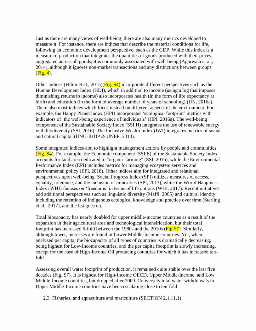
Just as there are many views of well-being, there are also many metrics developed to

measure it. For instance, there are indices that describe the material conditions for life,

following an economic development perspective, such as the GDP. While this index is a

measure of production that integrates the quantities of goods produced with their prices,

aggregated across all goods, it is commonly associated with well-being (Agarwala et al.,

2014), although it ignores non-market transactions and any distinctions between groups

(Fig. 4).

Other indices (Hilmi et al., 2015)(Fig. S4) incorporate different perspectives such as the

Human Development Index (HDI), which in addition to income (using a log that imposes

diminishing returns to income) also incorporates health (in the form of life expectancy at

birth) and education (in the form of average number of years of schooling) (UN, 2016a).

There also exist indices which focus instead on different aspects of the environment. For

example, the Happy Planet Index (HPI) incorporates ‘ecological footprint’ metrics with

indicators of ‘the well-being experience of individuals’ (HPI, 2016a). The well-being

component of the Sustainable Society Index (SSI.H) integrates the use of renewable energy

with biodiversity (SSI, 2016). The Inclusive Wealth Index (IWI) integrates metrics of social

and natural capital (UNU-IHDP & UNEP, 2014).

Some integrated indices aim to highlight management actions by people and communities

(Fig. S4). For example, the Economic component (SSI.E) of the Sustainable Society Index

accounts for land area dedicated to "organic farming" (SSI, 2016), while the Environmental

Performance Index (EPI) includes metrics for managing ecosystem services and

environmental policy (EPI, 2018). Other indices aim for integrated and relational

perspectives upon well-being. Social Progress Index (SPI) utilizes measures of access,

equality, tolerance, and the inclusion of minorities (SPI, 2017), while the World Happiness

Index (WHI) focuses on ‘freedoms’ in terms of life options (WHI, 2017). Recent initiatives

add additional perspectives such as linguistic diversity (Maffi, 2005) and cultural identity

including the retention of indigenous ecological knowledge and practice over time (Sterling

et al., 2017), and the list goes on.

Total biocapacity has nearly doubled for upper middle-income countries as a result of the

expansion in their agricultural area and technological intensification, but their total

footprint has increased 6-fold between the 1980s and the 2010s (Fig.S7). Similarly,

although lower, increases are found in Lower Middle-Income countries. Yet, when

analyzed per capita, the biocapacity of all types of countries is dramatically decreasing,

being highest for Low-Income countries, and the per capita footprint is slowly increasing,

except for the case of High-Income Oil producing countries for which it has increased ten-

fold.

Assessing overall water footprint of production, it remained quite stable over the last five

decades (Fig. S7). It is highest for High-Income OECD, Upper Middle-Income, and Low

Middle-Income countries, but dropped after 2000. Conversely total water withdrawals in

Upper Middle-Income countries have been escalating close to ten-fold.

2.3. Fisheries, and aquaculture and mariculture (SECTION 2.1.11.1)

Aquaculture has an expanding list of species with differential regional and economic value

importance. 575 aquatic species, including freshwater, seawater and brackish species,

contribute to aquaculture. Two-thirds (44.2 million tons) of total fish production were

finfish species grown from inland aquaculture (38.6 million tonnes) and mariculture (5.6

million tons) (FAO, 2014), followed by mollusks (30% of animals grown), and crustaceans

(4%) (FAO, 2006). Nearly 40% of the farmed species are carps and about 4% salmon or

tilapia. In OECD countries, aquaculture is predominantly dominated by high economic

value marine species such as salmon and oysters, while lower-value freshwater species

such as carp and catfish predominate in Asian production. Aquatic plants, mostly seaweeds,

are increasingly contributing to providing jobs (US$6.4 billion in 2014), largely in

developing and emerging economies, and are emerging as an ecologically friendly

alternative to the use of coastal and marine ecosystems (Cottier-Cook et al., 2016).

The production of aquafeed has increased 4 times to 29.2 million tons in 2008 (UN,

2016b), though no comprehensive information on farm-made aquafeeds and/or on the use

of low-value fish with low market value as fresh feed is available. Fishmeal and fish oil are

produced mainly from harvesting stocks of small, fast reproducing fish (e.g., anchovies,

small sardines and menhaden). This use was promoted in the 1950s by FAO as a means to

add value to the massive harvesting of small pelagic fish. Fishmeal is increasingly being

used as a strategic ingredient fed in stages of the growth cycle when its unique nutritional

properties can give the best results or in places where price is less critical. The most

commonly used alternative to fishmeal is soymeal.

2.4. Agriculture & Grazing (crops, livestock, agroforestry) (SECTION 2.1.11.2)

Several studies have shown the extensive and successful use of agroforestry, as a key

practice in agroecological approaches (Prabhu et al., 2015), to alter structural complexity of

coffee for increased functional diversity of avian insectivores, with increased removal of

about 50% of coffee berry borer (Hypothemus hampei) and improved management of

fungal pathogens (Avelino et al., 2016; Karp et al., 2013; Perfecto et al., 2014). Other

studies show agroforestry and soil conservation techniques at landscape level through

various incentive schemes have enabled improved soil erosion management, sediment

control and as a result more reliable power supply dams (DeClerck et al., 2010; Estrada-

Carmona & Declerck, 2012).

2.5. Forestry (logging for wood & biofuels) (SECTION 2.1.11.3)

Solid biofuel from woody plants, crop residue and dung is a primary source of energy. The

energy ladder suggests that poorest people use dung, agricultural waste, fuelwood and

charcoal as main sources of energy and that as affluence increases they replace these

gradually by wood, charcoal or kerosene stoves, and then by LPG and finally by electricity

(Masera et al., 2000). While bioenergy is starting to shift from a traditional and indigenous

energy source to a modern and globally traded commodity (GEA, 2012; IEA, 2016; World

Energy Council, 2016), solid biofuel is still the number one source of energy used by

households, contributing to 9.2% of world’s total energy supply in 2014 (IEA, 2017b).

Developing countries produced and use ~85% of biofuels in 2014, which are usually

burned in open fires or in inefficient and polluting stoves that typically emit smoke into the

indoor environment (IEA, 2016). Wood fuel, mainly firewood and charcoal, accounts for

the majority of solid biofuel used globally, while about half the wood extracted worldwide

from forests is used to produce energy. Crop residue and dung are also important solid

biofuels used by households in some rural developing regions, but no comprehensive global

statistics exist. Solid biofuel, especially wood fuel, is the primary source of residential

energy for around 2.7 billion people around the world, particularly in developing countries

in Sub-Saharan Africa and South Asia (De Stercke, 2014; IEA, 2016). More than 90% of

households in Sub-Saharan Africa depend on wood fuel for their daily cooking needs

(Cerutti et al., 2015). Africa accounted for only 5.6% of the world’s total primary energy

supply in 2014, but accounted for 29.3% of the world’s solid biofuels supply (IEA, 2017a)

and has always maintained the highest per capital bioenergy consumption (Chum et al.,

2011).

From 1961 to 2015, global wood fuel production increased by 25% from 1.5 billion m3 to

about 1.87 billion m3, mostly contributed by African countries (FAOSTAT, 2016). Asia-

Pacific was the largest producer (40%), followed by Africa (32%), Latin America and the

Caribbean (14%), Europe (8%) and North America (4%). The rates of global wood fuel

production peaked during the mid-1970s and since the 1980s the global increase in wood

fuel production slowed down for Upper Middle-Income countries (Fig. S17). Deforestation

and forest degradation in tropical regions and wood fuel extraction in Sub-Sahara Africa

were the main drivers (Rademaekers, Eichler, Berg, Obersteiner, & Havlik, 2010).

Between 27 and 34% of the global wood fuel harvest in 2009 was deemed unsustainable,

with large geographical variations, and ∼275 million rural people living in wood fuel

scarcity “hotspots,” mostly in South Asia and East Africa (Masera, Bailis, Drigo, Ghilardi,

& Ruiz-Mercado, 2015).

Charcoal is a transitional fuel, which is cleaner and easier to use than firewood and often

cheaper and more readily available than gas or electricity (van Dam & FAO, 2017). Global

charcoal production increased by more than 3-fold between 1961 and 2015 (FAOSTAT,

2016), due to population growth, poverty, urbanization and the relatively high prices of

alternate energy sources for cooking (van Dam & FAO, 2017). Of all the wood used as fuel

worldwide, about 17 percent is converted to charcoal. Africa currently accounts for 62% of

the global charcoal production, mostly in Sub-Saharan Africa. In many developing

countries across Southeast Asia and South America, wood for charcoal production is

sourced mainly from natural forests and woodlands, and usually produced using simple

technologies with low efficiency, resulting in substantial losses of wood and energy (van

Dam & FAO, 2017). Wood pellets production and consumption is the main wood fuel used

in Europe and North America (Schlesinger, 2018).

2.6. Mining: minerals, metals, oils and fossil fuels (SECTION 2.1.11.5)

Fossil fuel extraction has been marked by changes in fuel sources, fuel demand and fuel

prices. Accessibility to shale oil and gas has increased (Joskow, 2013) and many factors

regulate the fossil fuel markets (Baumeister & Kilian, 2016; Hamilton, 2009b; Kilian,

2009). Low gas prices brought on by the boom in shale gas production (Hausman &

Kellogg (2015), and oil price fluctuations are more driven by demand factors than supply

ones (Baumeister & Kilian 2016). Kilian (2016a, 2016b, 2017) found little effect on Brent

crude oil prices (although the surge in tight oil did contribute to the spread between the

prices of WTI and Brent crude oil during 2011-2014).

2.7. Infrastructure (dams, cities, roads) Urbanization and infrastructure (SECTION

2.1.11.6)

Urban expansion and economic growth are imposing major management challenges around

the world as illustrated here with the case of water (Liu & Yang, 2012; McDonald et al.,

2014). For instance, megacities (cities with populations over 10 million) constitute hotspots

of water use and face enormous water sustainability challenges (Engel et al., 2011; UN,

1998, 2010). Of 28 megacities that currently exist, 22 rely on distant water transfers (UN,

2014). These require development of large water infrastructure projects, with

socioeconomic and environmental effects across some large regions. The Three Gorges

Dam and the South-to-North Water transfer project constitute two of the largest such

projects, in the world, with consequences including biodiversity loss and human

displacement, among others, including land-use change (Fu et al., 2010; Liu, Yang, et al.,

2016). While these mega-projects benefit people in distant urban centers, their

socioeconomic burdens fall completely on rural areas that locally are directly affected, with

not only displacement but also drastic changes in livelihoods including negative economic

(e.g., loss of income, debt increase) and social (e.g., loss of social ties) impacts (Moore,

2014; Tilt & Gerkey, 2016; Wilmsen, Webber, & Duan, 2011; Wilmsen, 2017). Project

impacts also increase the vulnerability of rural people to any further external shocks

(Wilmsen et al., 2011)

2.8. Illegal activities with direct impacts on nature (SECTION 2.1.11.10)

IUU is highly lucrative for the high value of fishing demersal species (e.g. cod), as well as

salmon, trout, lobster and prawns, which are already overexploited by legal fishing or

subjected to restrictions for fisheries management, even if the quantities are small but the

prices are very high. Also, IUU does not pay taxes or duties on the catches. Interactions

between IUU and legal catch quotas in the maritime region and marine protected areas,

where a total fishing ban is imposed, are complex to asses. IUU fishing (http://www.dfo-

mpo.gc.ca/international/isu-iuu-drvrs-eng.htm) is promoted by weak governance of the

global commons. Efforts to enhance international fisheries and oceans governance have

come a long way in the last decade, resulting in significant improvements in the

management of high seas and highly migratory fish stocks. Yet, not all regions on the high

seas are overseen by a regional fishery management organization (RFMO), and not all

RFMOs are as effective in monitoring, controlling and surveilling their regulatory area to

prohibit IUU fishing. The Agreement on Port State Measures to Prevent, Deter and

Eliminate Illegal, Unreported and Unregulated Fishing (FAO, 2016), came into force in

June 2016, with 54 parties, all 28 members EU counted as one. The Marine Resources

Assessment Group (2005) states that the most obvious impact of IUU fishing is direct loss

of the value of the catches that could be taken by the coastal State otherwise. Vessels

operating without licenses and licensed vessels misreport catches (quantity, species, fishing

area, etc.) and illegal trans-shipment of catches (not much quantitative data on this one).

Secondary economic impacts from the loss of fish to IUU vessels include reduced revenue

from seafood exports and reduced employment in the harvest and postharvest sectors, and

conflicts and IUU fishing generally occur between vessels of any size. The endorsement of

170-member states of the FAO Code of Conduct for Responsible Fisheries (CCRF) in

1995, has contributed to decreases in IUU fishing. It was endorsed by around 170-member

states- and is voluntary and non-binding- countries. Australia, Malaysia, Namibia, Norway

and South Africa, have incorporated some of its provisions into national law.

Due to recent improvements in technology and affordability, vessel monitoring systems

(VMS) are increasingly available for both large- and small-scale fishing vessels, and thus

can provide geo-referenced data that accurately describe fishing areas on geographic scales

applicable to MSP (Global Fishing Watch, 2018; Kroodsma et al., 2018; Mccauley et al.,

2016). Such data can be combined with validated logbook data, rich time-series data are

potentially available from intensely fished and monitored sea areas, though largely for

developed countries. The data situation is slowly improving in developing countries. Land

tenure systems that extend to parcels of seabed and water for aquaculture also provide clear

boundaries. Superimposed on these spaces are increasingly sophisticated layers of

information on the interactions among fisheries, and between aquaculture and fisheries.

Although not all fisheries conflicts concern spatial use, or can be managed through MSP,

many are potential candidates for spatial conflict management.

2.9. Evolving economic & Environmental tradeoffs (SECTION 2.1.18.2)

Environmental justice focuses on “how the burdens of environmental harms and regulations

are allocated among individuals and groups within our society” (Salzman & Thompson,

2003, p. 38). The concept was developed in the United States, in struggles against waste

dumping in North Carolina in 1982. Activist-authors such as Robert Bullard, civil rights

activists with no academic affiliation, and members of Christian churches, like Benjamin

Chavis, saw themselves as militants of environmental justice (Martinez-Alier et al., 2014).

In a seminal work Dumping in the Dixie, (Bullard & Wright, 1990) examined the

environmental inequities that exist in the United States, particularly in the South: Texas,

Louisiana, West Virginia, and Alabama. He identified that polluting industries follow the

“path of least resistance” by locating their landfills, power plants, chemical plants, and

hazardous waste dumps in minority areas that are economically poor and politically

powerless. Although many interpret that environmental justice goes hand in hand with

environmental equity, in reality the concept of environmental justice is more politically

charged in the sense that it connotes some remedial action to correct an injustice imposed

on a specific group of people (Cutter, 1995).

During the last 3 decades, scholars, activists, social movements and even government

agencies, have produced extensive literature and evidence on the dimensions of differential

environmental risks based on race and low-income (Brulle & Pellow, 2006). One of the

first studies to perform a systematic meta-analysis of empirical studies shedding light on

race and class was Bryant & Mohai (1992). They analyzed 16 studies and found that race

was a more important predictor than income of where environmental hazards are located.

However, the multiple evidence (Bowen et al., 1995; Morello-Frosch et al., 2001; Pastor Jr

et al., 2002) show that environmental inequities in this context are a result of racism or

class barriers or a combination of both.

In other parts of the world, although the reality is different because people of color and

poor people are not minorities, environmental inequities reveal the same patterns. For

instance, in India caste has been an important aspect when analyzing disproportionate

amounts of pollution and other environmental stressors (Demaria, 2010; Parajuli, 1996). As

well, tribal affiliation often counts in many other countries in the struggles against resource

extraction. In Nigeria, Shell and other oil companies have shifted the social and

environmental costs of oil extraction onto indigenous, poor local communities (Martinez-

Alier et al., 2014).

Negative shocks to the economy and nature clearly also may occur e.g., from climate

change (regardless of cause), paraphrasing the IMF World Economic Outlook: Economic

costs of warming include: ‘market’ impacts upon climate-sensitive sectors (agriculture,

forestry, fisheries and tourism); damage to coastal areas from sea-level rise; higher

expenditures for heating or cooling; changes in water resources; and non-market impacts

such as the spread of infectious diseases, increases in water shortages, greater pollution and

damages to ecosystems. Prominent prior studies (Mendelsohn et al., 2000; Nordhaus &

Boyer, 2000; Tol, 2002) and literature covered in the Stern Review (2006) point to losses

between 0% and 3% percent of the world’s GDP, for a 3°C warming from 1990–2000

levels. Yet these estimates of damages rarely cover non-market damage, or the risk of local

extreme weather or large temperature increases and global catastrophes. Further, such

estimates of total global damages mask quite large variations − e.g., more damage for the

countries with higher initial temperatures, greater climate change, and lower levels of

development, which often implies greater dependence on climate-sensitive sectors and in

particular agriculture. The regions that are likely to experience the greatest negative effects

include Africa, south and southeast Asia (especially India), Latin America and the

European OECD. In contrast, China, North America, OECD Asia and all the transition

economies (especially Russia) should suffer smaller impacts and may even benefit.

Uncertainty plagues such damage estimates, however, starting from our limited scientific

knowledge concerning the physical and ecological processes that underlie climate change

and including how best to quantify economic impacts. The losses will depend on how well

people, firms and other institutions adapt − including the extent to which technological

innovations reduce impacts. Any such quantification of the aggregate losses across

generations involves some use of a specific welfare measure and it raises questions about

how changes in welfare in the future should be discounted (that is related to the return on

capital as a higher rate implies wealthier futures that we might worry less about per equity).

Weitzman (2007) argues that the most important source of variation is uncertainty about

catastrophes.

Such negative shocks to the economy and nature can, critically, affect health, usually

exacerbating existing inequalities and, as noted, potentially affecting growth. A myriad of

health impacts can occur from environmental transformations due to land-use change,

climate change, water scarcity, biodiversity loss, changing biogeochemical cycles

(Whitmee et al., 2015) and varied alterations of ecosystems and their services will

disproportionately affect poor populations in the developing world (Myers et al., 2013),

accentuating existing health inequities. Increasing carbon dioxide in the atmosphere will

reduce the micronutrient content of food crops (Myers et al., 2014), while a sea-temperature

rise will move fish polewards away from the food-insecure equatorial belt of nations;

Golden et al. (2016; 2017) note that aquaculture and mariculture can help with these

challenges but their production and distribution patterns are not designed for nutritionally

vulnerable nations. Deforestation and fragmentation in the Amazon could increase malaria

(Vittor et al., 2006) and, perhaps, also other devastating diseases such as Ebola and HIV

thought to have been released from African forests, while forest burning in Indonesia

generates severe air pollution and haze, driving increases in respiratory infections, maternal

mortality and cognitive deficits (Marlier et al., 2015).

Oil Palm

Palm oil production has been growing immensely in the last few decades. Production grew

from 37 Million Metric Tons in 2006 to 65 Million Metric Tons in 2016, and it is projected

to reach 85 Million Metric Tons in 2024. The global market value for palm oil and its

derivatives was estimated at 65.7 Billion USD in 2015 and estimated to reach 90 Billion in

2021.

This is fuelled by increasing demand for multiple uses. Most of the palm oil is used in the

food industry. It is widely used in frying and cooking oils, bakery, biscuit and pastry fats,

margarines, animal feed, confectionery filling, coffee whiteners, ice creams etc. More

traditional /non-food use has been in oleochemicals as a replacement for petroleum

products in soaps, detergents, greases, lubricants and candles. Fatty acid derivatives are also

used in producing pharmaceuticals, water-treatment products and bactericides. More

recently, it has been used as feedstocks for biodiesel production and as alternative to

mineral oils in power stations.

This global demand has been driven from emerging centers of international capital in the

Southern Hemisphere (Borras et al., 2016). This is being encouraged also by institutions

such as the World Bank (Deininger et al., 2011) and UNEP (Segura-Moran, 2011), under

the assumption that there are marginal (unpopulated) lands apt for cultivation and that

promoting the development of oil palm plantations as crops can help solve manifold

energy, climate, economic and financial crises. Governments envisage jobs and revenues

that could help mitigate high unemployment in developing countries and help supplement

declining revenues due to extended periods of falling commodity prices worldwide. Other

stakeholders especially private actors see an opportunity as a feedstock for biofuels.

About 80% of palm oil production happens in Indonesia and Malaysia, with the rest

distributed across Latin America (Colombia, Guatemala, Ecuador, Honduras and others)

and West Africa (Nigeria, Ghana, Cote D’Ivoire and others). However, palm oil production

area has been growing in Africa over the last few years, with Nigeria, Democratic Republic

of Congo (DRC), Ghana and Cote D' Ivoire being lead producers. In the Congo Basin, in

Cameroon the production increased from 21,000 tons in 1994 to 53,000 tons in 2010 (FAO,

2009; Hoyle and Levang, 2012), while the production in Gabon increased from 5,000 tons

in 1994 to 12,000 tons in 2007 (FAO, 2009). Top ten consumers include India, Indonesia,

EU, China, Pakistan, Nigeria, Thailand, Bangladesh and USA.

There is growing evidence that palm oil production (Elaeis guineensis), alongside soy,

beef, wood, cocoa, coffee and other cash crops account for a great deal of tropical

deforestation (up to 65%), alongside a number of other environmental and ecosystems

degradation challenges (Borras et al., 2011; Gibbs et al., 2010). In Latin America and

Southeast Asia this expansion has reduced soil fertility, increased water and air pollution

(caused by major fires) and biodiversity loss; and prevented communities from accessing

their main sources of livelihoods (water, fertile soil, food). The intensive use of pesticides

has caused ecological disasters such as the “ecocidio” (thousands of fish death) (EJAtlas,

2015). The fires and deforestation have increased the number of human infections and

premature death (Fornace et al 2016; Burrows 2016).

In Guatemala, cultivated lands with palm oil plantations increased almost 600% from 2000

to 2010 at the expense of the country’s tropical forests, wetlands and subsistence

agricultural land. The expansion has been driven by states, international institutions and

corporations and is controlled by five elite Guatemalan families allied to several

transnational groups (Alonso-Fradejas, 2012).

The deforestation and ecosystems degradation (such as peatlands in Indonesia) and other

environmental, and rights issues around oil palm production has triggered a number of

policy responses at multiple levels. The Roundtable for Sustainable Palm Oil (RSPO)

created in 2008 is probably the most well-known response (www.rspo.org). RSPO

pioneered a multistakeholder platform between producers, the consumer-oriented industry,

environmental and social NGO's and stakeholder groups and governments. This resulted in

a set of principles, criteria and indicators and a certification scheme aimed at regaining trust

between consumers and producers. The two main producer countries, Indonesia and

Malaysia, have followed these voluntary standards, and developed their own mandatory

system to enforce stronger compliance with the existing rules and regulations. RSPO has so

far certified about 11.7 Million Metric Tons (19% of global production) and currently has

membership from 91 countries.

The European Union has also taken specific measures given its position as the second

largest market of Indonesia’s palm oil after India. The EU instituted an Anti-dumping

Initiative regarding biodiesel from Indonesia and Argentina. EU lawmakers voted a law in

January 2018 to ban palm oil-based biofuels by 2021. Under the 2030 sustainable

development agenda, the EU is committed to halting deforestation, restoring degraded

forests and promoting sustainable procurement by 2020.

At national the top producing country, Indonesia is also considering other measures.

Proposed direct actions include a Peatland Restoration Agency for the purpose of restoring

two million hectares of fire-hit peatland and, while freezing new concessions, working

closely with other significant consumers of palm oil to raise awareness and to explore

common solutions to the problem of tropical deforestation and forest degradation.

It has been argued that the implementation of RSPO rules especially in Indonesia and

Malaysia and policy shifts in the EU demanding sustainable palm oil where rigorous

conditions, regulations and demands are forcing major plantation companies to shift

investments to Africa, where conditions are less stringent at the moment. This increased

production for export has been linked to disruption of the local values, nutrition, culture and

markets for palm oil in Congo Basin countries. Palm oil is the main edible oil in the region,

and is widely used for multiple medicinal uses. With rising global demand, the price of

palm oil has more than doubled in the region, increasing cost of living in the region. The

higher prices have in turn fueled local investments in oil palm. For instance, there is

evidence of growth and the establishment of medium-sized 5 - 50-hectare plantations in the

southern Cameroon forest areas due to return of urban investments by the Cameroonian

elite that increasingly see palm oil as a reliable and profitable investment (Yemefack et al.,

2005). These medium-sized producers largely target the local market, but prospects for

integrating out-grower schemes of large producers are very good.

The growth of palm oil in Africa has been associated with land grabbing in the Congo

Basin and the Guinea forest ecosystem, where several land acquisition deals for palm oil

production by multinationals have been reported (see www.landmatrix.org). While several

of the acquisitions remain undeveloped due to local community resistance and land claims,

where developments have proceeded as planned, the employment envisaged and high

revenues have been mixed because jobs are mostly low paid jobs and often short lived. Tax

exemptions, limited local financing opportunities and poor infrastructure sometimes limits

the economic gains envisaged by governments (Cotula, 2016).

It is evident that demand for palm oil will continue to grow and consequently, its

production will continue to increase. Several developing countries continue to see its

expansion as an opportunity to bring marginally profitable lands under palm oil production,

create jobs and improve revenues in the midst of a poor global outlook for commodities.

Likely negative impacts on nature and its benefit to people would continue if current

policies are not reinforced. Current certification efforts in oil palm only covers 19% of

global production with prospects for expansion limited by poor governance, capacity and

cost challenges in producing countries (Mithöfer et al., 2017). Consumer country measures

such as EU bans on imports of palm oil-based biodiesel only targets a small segment of

market. Hence, more far reaching policy responses are needed.

Managing landscapes in which palm oil is grown for multiple ecosystems services as well

as production is imperative given failed efforts to stop its growth. One key option could be

agroecological approaches- i.e. implementing ecological principles in the management of

agricultural lands. Agroecology applications to oil palm, especially agroforestry show

potential for simultaneously increasing productivity, profitability and maintaining or

enhancing ecosystem services. This might require multiple incentives including monetary

investments, subsidies, technical training and others (Minang, 2018) to enhance the abilities

of farmers and stakeholders manage working landscapes.

Estonia, the Soviet Union and the European Union

Active exploration of oil-shale deposites from Estonia did not occur until World War I

when there were fuel shortages.

After World War II, annual shale-oil production increased reaching its highest rates in 1980

(Dyni, 2003). As a result, Estonian oil shale gas was used in Saint Petersburg (then

Leningrad) and in northern cities in Estonia as a substitute for natural gas. With ongoing

industrial growth, there was increased need for electricity in the north-west of the Soviet

Union. This led to the construction of three large, oil-shale-fired power stations is Estonia

and oil-shale extraction peaked in 1980 at more than 30 million tonnes per year. A shift in

Soviet priority, though, involving the launch of nuclear reactors in Russia (particularly

Sosnovyi Bor), reduced demand for electricity produced from oil shale.

Post-Soviet function was quite different in key dimensions. For instance, the post-Soviet

restructuring of the electricity industry in the 1990s, led to a decrease in oil shale mining.

More recently, after decreasing for two decades, oil-shale mining started to increase again

at the beginning of the 21st century, implying a serious impact on the environment

including water and air pollution from extraction and processing. The combustion and

thermal processing generate waste requiring disposal, and atmospheric emissions

including carbon dioxide. In 2015, it produced about 70% of Estonia's ordinary waste, 82%

of its hazardous waste and more than 70% of its greenhouse gas emissions while lowering

groundwater levels and water quality

European governance brings yet another twist to this tale. While the Estonian National

Development Plan for the Utilisation of Oil Shale 2008–2015 prioritises oil shale as a

resource for ensuring Estonia's electricity supply and energy security, the share of oil shale

in Estonia's electricity and heat production is set to decrease due to the European Union's

climate policy and the country's recognition of the environmental impacts and a need to

diversify the national energy balance. While Estonia has the right to allocate a gradually

decreasing limited number of emission allowances free of charge, this will be phased out by

2020.According to the International Energy Agency, Estonia shou reduce the share of oil

shale in the primary energy supply by improving the efficiency of shale-fired power

stations and increasing the use of renewable energy and natural gas. All this involves other

countries in other ways as well. About 29% of produced electricity was exported to

Finland, Latvia, and Lithuania and during the 1990s Finland supported processes of

political and economic transition in neighbouring areas. Co-operation developed in

particular with those regions of Russia bordering on Finland and with Estonia, Latvia,

Lithuania and Poland. At the end of 2001, renovation of power plants began, with the

introduction of a new combustion technology – circulating fluidized bed (CFB) process.

Concentrations of SO2 and NOx in the flue gas from CFB power units are more than 100

and 2 times lower, respectively, fulfilling EU Directive 2001/80/EEC. Decline in SO2

emissions from oil-shale power in Estonia is an important factor in decreasing acidification

of lake water and forest soil in southern Finland as well as in Leningrad District in Russia

situated to the east from the town of Narva. Fiscal measures with an impact on GHG

emissions in Estonia include excise duties and pollution charges. As a Member State,

Estonia must comply with EU Directive 2003/96/EC for the taxation of fuels and energy.

While Estonia was granted a transitional period for the introduction of relevant taxes, e.g.,

regarding shale oil it was eligible for a transitional period until 1 January 2010 to adjust the

national level of taxation for district heating purposes, nevertheless Estonia had already

introduced the tax on shale oil by that date.

3. Selected recent critical references included in this report beyond the May 2018

threshold

Galaz, V., Crona, B., Dauriach, A., Jouffray, J.-B., Österblom, H., & Fichtner, J. (2018). Tax

havens and global environmental degradation. Nature Ecology & Evolution, 2(9), 1352–

1357. https://doi.org/10.1038/s41559-018-0497-3

Garnett, S. T., Burgess, N. D., Fa, J. E., Fernández-Llamazares, Á., Molnár, Z., Robinson, C. J.,

Watson, J. E. M., Zander, K. K., Austin, B., Brondizio, E. S., Collier, N. F., Duncan, T.,

Ellis, E., Geyle, H., Jackson, M. V., Jonas, H., Malmer, P., McGowan, B., Sivongxay, A.,

& Leiper, I. (2018). A spatial overview of the global importance of Indigenous lands for

conservation. Nature Sustainability, 1(7), 369–374. https://doi.org/10.1038/s41893-018-

0100-6

Lenzen, M., Sun, Y.-Y., Faturay, F., Ting, Y.-P., Geschke, A., & Malik, A. (2018). The carbon

footprint of global tourism. Nature Climate Change, 8(6), 522–528.

https://doi.org/10.1038/s41558-018-0141-x

IPCC. (2018). Global Warming of 1.5°C. An IPCC Special Report on the impacts of global

warming of 1.5°C above pre-industrial levels and related global greenhouse gas emission

pathways, in the context of strengthening the global response to the threat of climate

change, sustainable development, and efforts to eradicate poverty (V. Masson-Delmotte, P.

Zhai, H.-O. Pörtner, D. Roberts, J. Skea, P. R. Shukla, … Waterfield, Eds.). Geneva,

Switzerland: World Meteorological Organization.

Mazor, T., Doropoulos, C., Schwarzmueller, F., Gladish, D. W., Kumaran, N., Merkel, K., Di

Marco, M., & Gagic, V. (2018). Global mismatch of policy and research on drivers of

biodiversity loss. Nature Ecology & Evolution, 2(7), 1071–1074.

https://doi.org/10.1038/s41559-018-0563-x

Meyfroidt, P., Chowdhury, R. R., de Bremond, A., Ellis, E. C., Erb, K. H., Filatova, T., Garrett,

R. D., Grove, J. M., Heinimann, A., & Kuemmerle, T. (2018). Middle-range theories of

land system change. Global Environmental Change, 53, 52–67.

https://doi.org/10.1016/j.gloenvcha.2018.08.006

4. Methods for literature review

4.1. Key messages, outline and iterative literature review steps

The outline of the First Order Draft (FOD) was largely built through the analysis of the

outlines of the drivers sections of the Second Order Drafts (SOD) of the four regional

IPBES assessments (Americas, Africa, Europe and Central Asia, Asia Pacific).

The outline of the SOD was first built from FOD, comments from reviewers, the drivers

typology as well as revisions by the team of authors, and co-chairs. Then, it was revised

iteratively from the identification of key messages as they were iteratively identified and

refined.

The literature review was undertaken iteratively from three different complementary

processes that ran in parallel with the development of the outline of the FOD and the SOD:

1- identification of global policy relevant issues, 2- the in-depth analysis of the different

subsections, 3- global overview.

4.2. Global policy relevant issues

In order to identify the most salient global issues relevant to the Drivers sub-chapter we

revised the last ten years of the reports of relevant global organizations. These included:

FAO, UN, UNESCO, UNEP, World Bank, World Economic Forum, World Health

Organization, World Resources Institute. Within these reports we targeted the key policy

relevant messages as well as the supporting information (figures and tables).

4.3. In-depth analysis of the different subsections

Each of the subsections of the outline (e.g. 4.1.1.) was led by one of the CLAs or LAs,

based on their previous knowledge on the specific topic. The aim was to produce a short

and critical, analysis of the most relevant issues and their complex interlinkages, based on

an assessment of the available literature. To support this task, we invited a wide range of

contributing authors (CAs) from different disciplines and countries. This wide team of CAs

would be able to convey a diversity of approaches and perspectives. We targeted scholars

with well-known experience on these topics, as well as early career academics that were

deeply familiar with the corresponding literature and issues.

The in-depth analysis was based on a wide range of literature sources, including those not

easily accessible through systematic literature review such as that associated to relevant

study cases, books and reports in several languages beyond English.

4.4. Global overview

To complement the in-depth analysis, we also searched for literature that would provide a

global overview of the different subsections, when needed. To do so we piloted a

systematic review per subsection using Publish or Perish

(http://www.harzing.com/resources/publish-or-perish) for the case of each of the activities

with direct impacts on nature (4.1.1 to 4.1.9). The search retrieved a very large number of

papers (100-200) per subsection (e.g. 4.1.1), but of which very few (< 5) provided the

global overview we expected to build to complement the in-depth analysis.

Instead, we dissected the literature search task into the specific topics that were identified

from the in-depth analysis and from the outline development, within each subsection (1-3

paragraphs). For that purpose we used google scholar. We targeted either of the following

papers: reviews, most recent, highly cited, global coverage, in high impact factor journals

(e.g. Science, Nature, PNAS).

Relevant books and reports were also retrieved from this exercise. Most reports were easily

downloadable, and complemented the identification of global policy relevant issues. Books,

which contributed to the global overview and to the in-depth analysis, were not always

accessible, depending on the respective online library subscriptions of the team of CLAs

and LAs.

4.5. Systematic assessment of the amount of literature available on interactions between

indirect drivers, actions and direct drivers

Articles retrieval. Bibliographic data were extracted from the Web of Science

(http://apps.webofknowledge.com/WOS_GeneralSearch_input.do?product= WOS&search_

mode= GeneralSearch&SID= C62QZMbzHJ59XeiWLnq&preferencesSaved=; retrieved 5

October 2018). We extracted 206,956 articles from 38 leading interdisciplinary journals

between January 2017 and October 2018 (with 2017 impact factor > 3.16). We used a filter

of 166 keywords that referred to nature and reduced the total number of analyzed papers to

a sample of 48,892 articles. For these articles we obtained information on keywords,

authors, title, abstract, year of publication and journal. All bibliographic data were imported

into a database in R using the bibliometrix package (http://www.bibliometrix.org/).

Articles classification. Journal articles were classified into five direct drivers (climate

change, land/ seascape change, pollution, resource extraction, invasive alien species) and in

eight indirect drivers (actions, economic, development pathways, institutions and

governance, demographic, lifestyle and inequalities, technological and values). Articles

were classified based on the occurrence of direct and indirect drivers-specific words with

their respective title, keywords and abstract (Mazor et al., 2018)

The set of drivers-specific keywords (see tables below) was determined by extracting the

1,429 most frequently used keywords from all considered articles and assigning each word

to each direct and indirect driver. The set of driver search words was determined based on

the top 100 keywords of articles containing the explicit driver (for example, “climate

change”) in either the title, abstract or keywords. Each set of 100 words was filtered, using

only those words that >50% of the current authors agreed related to a driver. A total of

167,852 articles (81%) were assigned to one or more drivers.

Validation. We corroborated our procedure by manually inspecting 2.8% of the articles

across driver’s classification. 84% of the human-reviewed articles were successfully

categorized.

Analysis. We used social network analysis (Wasserman & Faust 1994) to assess the

contributions of indirect drivers to direct drivers of biodiversity and ecosystem services

loss. We built a network data set where n x n matrix S, where n equals the number of nodes

in the analysis and sij is the measured relation between specific nodes i and j. The node is

the unit of analysis. In this study, nodes represent direct and indirect drivers. Links are

based on the number of articles addressing the respective two connected drivers.

Table 1. Set of 1,429 keywords used to classify the literature addressing the indirect and

direct drivers

Topic Keywords

Direct

drivers:

Pollution

"pollution", "eutrophication", "ecotoxicology", "contamination", "pollute", "pollutes",

"pollutant", "polluting", “municipal waste”, “nitrogen deposition”, “chemical

pollution”, “hazardous substances”, “poor air quality”, “waste water dumps”,

“wastewater”, “asbestos”, “pesticides”, “open waste dumps”, “dump sites”, “solid

waste management”. “controlled waste disposal facilities”, “heavy metals”, “persistent

organic pollutants”, “endocrine-disrupting chemicals”, “micro-pollutants”, “waste

landfills”, “hazardous chemicals”, “e-waste”, “food waste”, “organic waste”,

“construction waste”, “demolition waste”, “hazardous waste”, “, “sulfur dioxide”,

“nitrogen oxides”, particulate matter 2.5”, “carbon monoxide”, “volatile organic

compounds”, “ammonia”, “plastic debris”, “fumaric acids”, “phthalic acids”,

“nitrates”, “phosphates”, “leachates”, “PCBs”, “floating plastic debris”, “GCC”,

“greenhouse gases”, “GHGs”, “greenhouse gas”, “GHG”, "carbon dioxide"

Direct

drivers:

Land/

seascape

change

"habitat change", "habitat-change", "habitat loss", "habitat-loss", "deforestation",

"fragmentation", "land-use change" “land use”, "forest fragmentation", "habitat

fragmentation", "habitat modification", "landscape change", , “urbanisation”,

“urbanization”, “agricultural expansion”, “urban expansion”, “crop lands expansion”,

“grazing lands expansion”, “infrastructure development”, “intensified land

management systems”, “tree plantation”, “tree plantations”, “industrial development”,

“agroforestry”, “human encroachment”, “managed forest”, “transformation of natural

ecosystems”, “human use-dominated ecosystems”. “anthromes”, “anthropic biomes”,

“road construction”, , “road expansion”, “dam construction”, “port construction”, “sea-

ice change”, “seascape change”, “change in seascape”, “changes in seascape patterns”,

“loss of coastal habitats”, “degradation of coastal habitats”, “loss of coral reefs”, “loss

of seagrasses”, “loss of mangroves”, “loss of salt marshes”, “changes in seascape

structure”, “fragmentation of seascape”, “loss of wetlands”, “large-scale conversion of

coastal wetlands”, “loss of inland natural wetlands”, “land use and land use change”

“LULUC”, “changes in sediment flows”, “reduction in sediment inputs”, “urban land

expansion”, “monoculture plantations”, “land degradation”, “degraded land”, “soil

degradation”, “surface sealing”, “soil compaction”, “soil acidification”, “soil fertility

loss”, “organic matter depletion”, “rangeland degradation”, “freshwater degradation”,

“soil erosion”, “forest degradation”, “loss of wetlands”, “loss of hydrological

functions”, “irreversible land degradation”,)

Direct

drivers:

Resource

extraction

“biomass extraction”, “biomass materials extraction”, “resource extraction”, “raw

material extraction”, “domestic extraction”, “harvested biomass”, “grazed biomass”,

“animal biomass extraction”, “plant-based biomass extraction”, “metallic minerals

extraction”, “gold extraction”, “non-metallic minerals extraction”, “sand extraction”,

“gravel extraction”, “limestone extraction”, “clays extraction”, “non-metallic minerals

extraction”, “fossil energy carriers extraction”, “coal extraction”, “crude oil

extraction”, “natural gas extraction”, “shale gas extraction”, “hydrated gas extraction”,

“shale oil extraction”, “timber extraction”, “construction materials extraction”, “fossil

fuels extraction”, “groundwater extraction”, “surface water extraction”, “fuelwood

collection”, “non-timber natural resource extraction”, “extractive industry”, “wood

extraction”, “charcoal extraction”, “ecosystem-derived fuels extraction”, “fuelwood

extraction”, “material footprint”, "overfishing", "overexploitation", "overgrazing",

"overhunting", "overharvesting", "over fishing", "over exploitation", "over grazing",

"over hunting", "over harvesting", "over-fishing", "over-exploitation", "over-grazing",

"over-hunting", "over-harvesting", "over fished", "over exploited", "over hunted",

"over grazed", "over harvested", "over-fished", "over-exploited", "over-hunted", "over-

grazed", "over-harvested", "overfished", "overexploited", "overhunted", "overgrazed",

"overharvested"

Direct

drivers:

Climate

change

"climate change", "global warming", "ocean acidification", "climate warming", “global

climate change”, “glacier retreat”, “extreme weather events and climate change”,

“LST” ,“sea-level rise”, “SLR”, “sea level rise”, “climate change effects”, “impacts of

climate change”, “black carbon”, “ocean acidification”

Direct

drivers:

Invasive

alien species

"invasive species", "biological invasion", "invasive", "invasion", "invasion ecology",

"alien species", "introduced species", "invasive plants", "invasions”, “non-native

species", "invasiveness", "invasibility", “emerging alien species”

Indirect

drivers:

Actions

“fisheries”, “aquaculture”, “industrial fishing”, “fish stocks”, “marine fisheries”,

“shrimp farming”, “salmon farming”, “agriculture”, “crop production”, “fertilization”,

“agricultural expansion”, “cattle”, “agricultural intensification”, “livestock”, “pasture”,

“food crops”, “grazing lands”, “agricultural systems”, “logging”, “wood fuel harvest”,

“firewood”, “charcoal”, “bioenergy”, “non-timber forest products”, “timber”,

“sustainable community forestry”, “mining”, “fossil fuel production”, “small-scale

mining”, “large mining multinationals”, “surface mining”, “gold mining”, “shale oil”,

“shale gas”, “offshore oil”, “offshore gas”, “seabed mining”, “marine mining”, “dams”,

“reservoirs”, “hydropower generation”, “illegal activities”, “illegal fishing”,

“unreported and unregulated fishing”, “illegal forestry”, “illegal logging”, “illegal

logging”, “illegal poaching”, “tourism”, “ecotourism”, “nature-based tourism”,

“sustainable tourism”, “wildlife-base tourism”, “adventure tourism”, “community

based ecotourism”, “ecosystem management”, “ecosystem conservation”,

“restoration”, “air flights”, “goods transportation”

Indirect

drivers:

Economic

"international trade", “globalization”, “economy”, “economic”, “production of goods”,

“GDP”, “markets”, “economic assets”, “income”, “import of goods”, “export of

goods”, “socioeconomic”, “socio-economic”, “financial flows”, “structural changes in

economies”, “economic transitions”, “production of goods”, “environmental kuznets

curve”, “materials flow”, “goods flow”, “land grabbing”, “water grabbing”

Indirect

drivers:

Demographic

"human migration", “human population”, “population growth”, “education”, “human

capital”, “megacities”, “decline of fertility”, “survival rates”, “death rates”, “size of

global population”, “global population”, “international migrants”, “international

migration”, “refugees”, “net migration”, “aging population”, “aged population”, “urban

population”, “rural population”, “growth in the urban population”, “urban dwellers”,

“settlements”, “urban growth”, “cities”, “urban development”, “rural-urban migration”

Indirect

drivers:

Technologica

l

“technological innovation”, “technologies”, “technology”, “green revolution”,

“genetically modified organisms”, “genetic engineered crops”, “genetically modified

seeds”, “insect resistance”, “herbicide tolerance”, “Big data”, “The internet of things”,

“IoT”, “artificial intelligence”, “3D printing”, “biotechnology”, “nanotechnology”,

“renewable energy”, “drones”, “satellite”, “frontier technologies”, “automation”,

“digital automation”, “data visualization”, interactive mapping”, “synthetic biology”,

“research and development”, “R&D” “patent”, “patent applications”, “technology

clusters”, “Science Technology and Innovation”, “STI”, “science, technology

engineering and mathematics”, “STEM”, “smart specialization, “technology parks”,

“PEDs”, “Global collaboration in scientific research”, “biotech”, “digital

technologies”, “nano-tech”, “green technologies”, “smart agriculture”, “smart

electricity grids”, “solar energy”, “smart grids”, “solar desalination”, “energy

efficiency”

Indirect

drivers:

Institutions

and

governance

“common-pool resource”, “collective property”, “local institutions”, “local natural

resources”, “social networks”, “collective tenure”, “corruption”, “revolving doors”,

“political stability”, “state take-over by corporations”, “Voluntary Partnership

Agreements”, “VPAs”, “co-management”, “common rights”, “human communities”,

“local human communities” , “collective rights”, “informal governance”, “collective

action”, “collaboration”, “coordination”, “community lands”, , “common-property

regimes”, “land rights”, “land tenure”, “community-based management”, “social

capital”, “local institutions”, “collective ejido tenure”, “governance”, “small scale

fisheries”, “public participation”, “forest certification”, “FSC”, “Stewardship”,

“certification”, “Market-based certification”, “Marine Stewardship Council”, “FSC

Certified Forest Area”, “certification principles”, “certification standards”,

“environmental policy”, “conservation policy”, “local government”, “national

government”, “policy choices”, “policies”, “political decisions”, “climate-change

policy”, “environmental policies”, “natural resource policies”, “policy solutions”,

“environmental regulations”, “environmental laws”, “Payments for Ecosystem

Services”, “Payments for Environmental Services” “biodiversity offset”,

“environmental taxes”, “policy spillovers”, “policy instruments”, “carbon taxes”,

“carbon tax”, “cap-and-trade”, “natural gas taxes”, “trade tariffs”, “agricultural

subsidies”, “Global North”, “Global South”, “world heritages sites”, “international

convention”, “CITES”, “CBD”, “IPCC”, “global coordination”, “global resource

domains”, “Ramsar sites”, “United Nations Framework Convention on Climate

Change”, “Montreal Protocol”, “Convention Biological Diversity”, “Conservation of

Antarctic Marine Living Resources”, “Nagoya Protocol”, “International cooperation”,

“Ramsar Convention on Wetlands of International Importance”, “Wetland

Convention”, “global treaties”, “global agreements”, “The Helsinki Rules on Uses of

the Waters of International Rivers”, “International Law Association”, “Johnston

Agreement”, “Indus Waters Treaty”, “Convention on the Protection and Use of

Transboundary Watercourses and International Lakes”, “International Council for the

Exploration of the Sea”, “Regional Fisheries Management Organizations”, “RFMOs”,

“United Nations Conference on the Law of the Sea”, “United Nations Convention on

Fishing and Conservation of Living Resources of the High Seas”, “Convention on the

Conservation of Antarctic Marine Living Resources”, “Kyoto Protocol”, “CITES”,

“program to monitor the illegal killing of elephants”, “IUCN”, “International Union

for Conservation of Nature”, “Roundtable for Sustainable Palm Oil”, “RSPO”,

“REDD+”, “REDD”, “Reducing emissions from deforestation and forest degradation”,

“Indigenous Peoples and Local Communities, IPLC”

Indirect

drivers:

Lifestyles

and

inequalities

"human well-being", “well-being”, “wellbeing”, “human wellbeing”, “quality of life”,

“consumption lifestyles”, “Western-style diets”, “waste generation”, “multidimensional

poverty index”, “MPI”, “poverty”, , “livelihoods”, “food security”, “access to water”,

“access to safe drinking water”, “maternal mortality”, “child mortality”, “death of

children under five”, “access to sanitation”, “access to electricity”, “local livelihoods”,

“inequality”, “social inequality”, “environmental justice”, “environmental inequities”,

“environmental hazards”, “human footprint”, “human footprint index”, “water

footprint”, “GDP per capita”, “the Human Development Index”, “HDI”, “OECD’s

Better Life Index”, “GPI”, “Genuine progress indicator”, “least developed countries”,

“LDCs”, “access to reproductive health care services”, “life expectancy”, “under-five

mortality rate”, “physical security”, “food security”, “water security”, “energy

security”

Indirect

drivers:

Values

“multiple values of nature”, “nature contributions to people”, “nature’s benefits”,

“nature’s benefits to people”, “good quality of life”, “instrumental values”, “monetary

value”, “materialist view”, “environmental values”, “nature-based spiritualities”,

“inherent values”, “intrinsic values”, “relational values”, “biocultural diversity”,

“biophilia”, “sense of place”, “sense of community”, “self-determination”, “sacred

sites”, “totemic beings”, “spiritual well-being”, “intra-generational equity”, “inter-

generational equity”, “plural values”, “sacred space”, “worldviews”, “expressions of

value preferences”, “moral judgments”, “cosmocentric”, “biocentric”, “biocentrism”,

“ecocentric”, “good quality of life” “animal welfare”, “animal rights”, “anthropocentric

values”, “non-anthropocentric values” “human thought”, “human emotion”, “human

expression”, “human behavior”, “cultural heritage”, “economic potential”, “biological

uniqueness”, “ecotourism”, “psychological benefits”, “bequest value” “rights to

nature”, “indigenous and local knowledge”, “ILK”, “cultural diversity”, “traditions”,

“rituals”, “mother earth rights”, “living well”, “ecological solidarity”, “systems of life”,

“customary uses”, “social capital”, “indigenous peoples”, “indigenous communities”,

“shared norms”, “stewardship”, “community cohesion”, “social resilience”,).

Indirect

drivers:

Development

pathways

“feedbacks”, “negative loop holes”, “integrated approaches”, “integrated decision

making”, “multiple sources of uncertainty”, “regime shifts”, “interactions drivers”,

“negative loop holes”, “abrupt changes”, “persistent changes”, “algae dominated

reefs”, “productivity decline”, “hypoxia”, “arctic sea ice”, “tipping point”, “tipping

points”, “lifeless zones”, “non-linear change”, “arctic regime shifts”, “loss of

ecosystem services”, “biodiversity loss”, “cultural identity loss”, “loss of species

richness”, “local knowledge loss”, “land abandonment”, “biodiversity degradation”,

“violent conflict”, “environmental conflicts”, “mining conflicts”, “unsustainable land

management”, “water depletion”, “eutrophication”, “hypertrophication”, “resistance to

antibiotics”, “chronic diseases”, “epidemic outbreaks”, “infectious diseases”,

“cardiovascular diseases”, “respiratory diseases”, “pneumonia”, “diarrheal diseases”,

“health impacts”, “global health threats”, “vulnerability”, “human appropriation”,

“human appropriation of net primary production”, “HANPP”, “anthropogenic

impacts”, “water shortages”, “water scarcity”, “cumulative environmental impacts”,

“transboundary use of resources”, “social-ecological resilience”, “sustainability”,

“social sustainability”, “economic sustainability”, “ecological sustainability”, “tele

coupling”, “teleconnections”, “embedded flows”

5. Data acquisition

5.1. Core and highlighted IPBES indicators

We worked closely with the Knowledge and Data Technical Support Unit of IPBES

(K&DTSU) to gather data on all relevant core and highlighted indicators for which data

was readily available https://www.ipbes.net/indicators. Through the K&DTSU we

requested the data that was not readily available from data providers with no success.

5.2. Publicly available data

We identified additional publicly available data from globally recognized resources: World

Bank, OECD, FAO, UNDP, NASA. Additionally, we identified particularly relevant public

data sources supported by Universities or well-known organizations on specific topics such

as the material flows data base http://www.materialflows.net/materialflowsnet/data/data-

download/.

5.3. Data bases contributed by contributing authors

Some CAs provided data bases that were supported by their publications.

6. Data analysis

6.1. Trends

Temporal trends within 1960 and 2015 where calculated for all the available variables for

the available dates. Global averages or totals, as well as averages among countries grouped

into World Bank Income Levels (see 6 below

https://datahelpdesk.worldbank.org/knowledgebase/articles/906519-world-bank-country-

and-lending-groups), and IPBES regions (see 6 below and

https://www.ipbes.net/dataset/ipbes-regions-subregions).

Two different procedures were applied to individual country data. We only included

countries with more than 5 years of temporal data onwards.

Doted lines in trends figures represent periods for which either no data is available between

the two extremes of the dotted line, or those for which the data presents very large

variability respective to that found in other periods within the same figure.

Synthesis figures with multiple variables with the same axis were prepared by standardizing

the response variables relative to a same shared year, for which a value of 1 (or 100) was

used as reference for all the variables.

The pollution indicators uses best available data on emissions of pollutants into the air,

water and soil: fertilizer use, lack of sanitation, greenhouse gas emission, municipal waste

production (per capita*population), pesticides use, air pollution by PM2.5 particles. Trends

in pollution were based on a synthesis indicator for which each of the above variables are

standardized using a value of 1 for the year 2000. Trends in air pollution, using only data

on greenhouse gas emissions and PM2.5 particles

6.2. Maps

6.2.1. Static

Selected variables were represented into maps for most recently available year.

6.2.2. Trends

Temporal trends of different metrics (i.e., variables of economic development,

globalization, air pollution, material extraction) were calculated for each country, using

linear regression against time (measured in years). Countries with insufficient data to

calculate the regressions were excluded. The slopes of these regressions were binned

among countries using natural breaks and the resultant bins were displayed in choropleth

maps. To aggregate different variables into a single metric, the slopes of the regressions for

each variable were first standardized across countries and then averaged among the

variables to be aggregated. These averages (in units of standard deviation) were then binned

among countries using natural breaks and the resultant bins were displayed in choropleth

maps.

The speed of temperature change (km yr-1) was calculated based on 30-arcsec WorldClim

Version 1.4 Annual Mean Temperature and Total Annual Precipitation bioclimatic variable

using the methods described in (Loarie et al., 2009).

Changes in the proportion of land cover in Urban and Cultivated Areas between year 1992

and year 2015 were calculated using the changes in the proportion of ESA CCI LandCover

in Urban (class value 190) and Cultivate Areas (Class values 10, 20, 30, and 40) in

gradients of white (no change) to dark red (100%). The proportion calculated based on the

number of Urban and Cultivated 300m cells within a grid of 10km.

The increase in total numbers of established alien species from 1950 to 2000. Species

numbers are indicated by color and additionally by circle size for islands with small land

areas. The years of first record of an alien species in a country or on an island are obtained

from the recent version of the Alien Species First Record Database (Seebens et al., 2018).

6.3. Meta-analysis

A preliminary meta-analysis was undertaken to compare among countries, classified into

income categories or into IPBES regions, the rate of change from 1980 to 2015 of the

response variables assessed, measured in some quantitative scale. We used in this pilot

analysis the total biomass extraction, GDP and air departures.

From the raw mean for each quantitative variable in each country we estimated the annual

rate. We thus included these values in a random-effects mixed model to evaluate

differences among income country groups (Koricheva et al., 2013). Models assumed a

normal distribution of data and a constant annual rate, through time. Each variable was

analyzed through its corresponding period of time (which varies among 1960 – 2016, 1980

– 2013, and other periods).

Figures show the predicted annual rates by the meta-analytic model. All figures show

mean values and standard errors. The dotted line represents global values. Standard errors

that not overlap mean statistical differences with p < 0.05. We used the metaphor package

in R (Viechtbauer, 2010).

We must further check for ratio scale measurements for nonlinear variables (many could be

nonlinear. For ratio scale measurements, the log transformed mean or the log transformed

coefficient of variation (with bias correction) may also be of interest (Nakagawa et al.,

2017). We also need checking by sample size (number of countries in each income

category), but at least at this point results are strong evident.

6.4. Synthesis pathways

All the quantitative and qualitative information gathered along the chapter was summarized

in two synthesis figures. They emphasize the mains contrasts in development pathways and

consequences for nature among higher income and lower income countries.

7. Data sources

Table 2. The indicators used and the data sources

Indicator Data source Description of the indicator

GDP

https://data.worldbank.o

rg/indicator/NY.GDP.

MKTP.CD

GDP at purchasers prices is the sum of gross value added by all

resident producers in the economy plus any product taxes and

minus any subsidies not included in the value of the products. It

is calculated without making deductions for depreciation of

fabricated assets or for depletion and degradation of natural

resources. Data are in current U.S. dollars. Dollar figures for

GDP are converted from domestic currencies using single year

official exchange rates. For a few countries where the official

exchange rate does not reflect the rate effectively applied to

actual foreign exchange transactions, an alternative conversion

factor is used.

Globalizat

ion index

https://www.kof.ethz.ch

/en/forecasts-and-

indicators/indicators/ko

f-globalisation-

index.html

The KOF Globalization Index measures the economic, social

and political dimensions of globalization. Globalization in the

economic, social and political fields has been on the rise since

the 1970s, receiving a particular boost after the end of the Cold

War.

Poverty

gap

https://data.worldbank.o

rg/indicator/SI.POV.G

APS

Average of Poverty headcount ratio at $1.90 a day is the

percentage of the population living on less than $1.90 a day at

2011 international prices. As a result of revisions in PPP

exchange, from 1986 to 2015

Food

Security

Index

http://foodsecurityindex

.eiu.com/

The Global Food Security Index considers the core issues of

affordability, availability, and quality across a set of 113

countries. The index is a dynamic quantitative and qualitative

benchmarking model, constructed from 28 unique indicators,

that measures these drivers of food security across both

developing and developed countries.

This index is the first to examine food security

comprehensively across the three internationally established

dimensions. Moreover, the study looks beyond hunger to the

underlying factors affecting food insecurity. This year the GFSI

includes an adjustment factor on natural resources and

resilience. This new category assesses a country's exposure to

the impacts of a changing climate; its susceptibility to natural

resource risks; and how the country is adapting to these risks.

Depth of

the food

deficit

(kcal/capit

a/day) (3-

year

average)

https://landportal.org/bo

ok/indicators/indfaofsec

6

The depth of the food deficit indicates how many calories

would be needed to lift the undernourished from their status,

everything else being constant. The average intensity of food

deprivation of the undernourished, estimated as the difference

between the average dietary energy requirement and the

average dietary energy consumption of the undernourished

population (food-deprived), is multiplied by the number of

undernourished to provide an estimate of the total food deficit

in the country, which is then normalized by the total

population.

Indicator Data source Description of the indicator

Access to

improved

sanitation

facilities

https://data.worldbank.o

rg/indicator/SH.STA.S

MSS.ZS

The percentage of people using improved sanitation facilities

that are not shared with other households and where excreta are

safely disposed of in situ or transported and treated offsite.

Improved sanitation facilities include flush/pour flush to piped

sewer systems, septic tanks or pit latrines: ventilated improved

pit latrines, compositing toilets or pit latrines with slabs

Domestic

Material

Consumpti

on

http://www.materialflo

ws.net/materialflowsnet

/data/data-download/

This category refers to the origin and/or destination of material

flows, as materials used by the economy can either be extracted

from the domestic territory or imported from other countries.

Note that for the categories of unused and indirect material

flows related to internationally traded products, the terms

„ecological rucksacks" and „hidden flows" are also used.

per capita

calorie

intake

https://ourworldindata.o

rg/food-per-person

The Coefficient of Variation (CV) of the per capita caloric

intake in a given population. The coefficient variation

(CV)measures the inequality of caloric intake across a given

population. It represents the a statistical measure of the

dataspread around the mean caloric intake. Higher CV values

represent larger levels of dietary inequality. The CV of

caloricintake is reported only for developing countries within

the Food Security Indicators

Prevalence

of obesity

in the

adult

population

(18 years

and older)

https://ourworldindata.o

rg/obesity

Percentage of adults aged 18+ years old who are defined as

obese based on their body-mass index (BMI). BMI is aperson's

weight in kilograms (kg) divided by his or her height in metres

squared. A BMI >30 is defined as obese.

Energy

use (kg of

oil

equivalent

per capita)

https://data.worldbank.o

rg/indicator/EG.USE.P

CAP.KG.OE?view=cha

rt

Energy use refers to use of primary energy before

transformation to other end-use fuels, which is equal to

indigenous production plus imports and stock changes, minus

exports and fuels supplied to ships and aircraft engaged in

international transport

Mobile

cellular

subscriptio

ns

https://data.worldbank.o

rg/indicator/IT.CEL.SE

TS.P2?

Mobile cellular telephone subscriptions are subscriptions to a

public mobile telephone service that provide access to the

PSTN using cellular technology. The indicator includes (and is

split into) the number of postpaid subscriptions, and the number

of active prepaid accounts (i.e. that have been used during the

last three months). The indicator applies to all mobile cellular

subscriptions that offer voice communications. It excludes

subscriptions via data cards or USB modems, subscriptions to

public mobile data services, private trunked mobile radio,

telepoint, radio paging and telemetry services.

Indicator Data source Description of the indicator

Fossil fuel

energy

consumpti

on (% of

total)

https://data.worldbank.o

rg/indicator/EG.USE.C

OMM.FO.ZS?view=ch

art

Fossil fuel comprises coal, oil, petroleum, and natural gas

products

Renewabl

e

electricity

consumpti

on (% of

total

electricity

output)

https://data.worldbank.o

rg/indicator/EG.ELC.R

NEW.ZS?view=chart

Renewable electricity is the share of electrity generated by

renewable power plants in total electricity generated by all

types of plants

Electric

power

consumpti

on (kWh

per capita)

https://data.worldbank.o

rg/indicator/EG.USE.E

LEC.KH.PC?view=char

t

Electric power consumption measures the production of power

plants and combined heat and power plants less transmission,

distribution, and transformation losses and own use by heat and

power plants.

Access to

electricity

https://data.worldbank.o

rg/indicator/EG.ELC.A

CCS.ZS?view=chart

Access to electricity is the percentage of population with access

to electricity. Electrification data are collected from industry,

national surveys and international sources.

Alternativ

e and

nuclear

energy (%

of total

energy

use)

https://data.worldbank.o

rg/indicator/EG.USE.C

OMM.CL.ZS?view=ch

art

Clean energy is noncarbohydrate energy that does not produce

carbon dioxide when generated. It includes hydropower and

nuclear, geothermal, and solar power, among others.

Protein

intake per

country

per person

http://chartsbin.com/vie

w/1155

This map shows dietary protein consumption per person. The

dietary protein consumption per person is the amount of protein

in food, in grams per day, for each individual in the total

population.

Energy

supply

derived

from

cereals,

roots and

tubers

http://www.fao.org/faos

tat/en/#data/FS

For detailed description of the indicators below see attached

document: Average Dietary Supply Adequacy; Average Value

of Food Production; Share of Dietary Energy Supply Derived

from Cereals, Roots and Tubers; Average Protein Supply;

Average Supply of Protein of Animal Origin; Percent of paved

roads over total roads; Road Density (per 100 square km of

land area); Rail lines Density (per 100 square km of land area);

Domestic Food Price Level Index; Percentage of Population

with Access to Improved Drinking Water Sources; Percentage

of Population with Access to Sanitation Facilities; Cereal

Import Dependency Ratio; Percent of Arable Land Equipped

for Irrigation; Value of Food Imports in Total Merchandise

Indicator Data source Description of the indicator

Exports; Political stability and absence of violence; Domestic

Food Price Volatility Index; Per capita food production

variability; Per capita food supply variability; Prevalence of

Undernourishment; Share of Food Expenditures of the Poor;

Depth of the Food Deficit; Prevalence of Food Inadequacy;

Children aged <5 years wasted (%); Children aged <5 years

stunted (%); Children aged <5 years underweight (%);

Percentage of adults underweight in total adult population;

Prevalence of anaemia among children under 5 years of age;

Prevalence of Vitamin A deficiency in the population;

Prevalence of Iodine deficiency; Prevalence of anaemia among

pregnant women; Number of people undernourished; Minimum

Dietary Energy Requirement (MDER); Average Dietary Energy

Requirement (ADER); "Minimum Dietary Energy Requirement

(MDER) - PAL 1.75"; Coefficient of variation of habitual

caloric consumption distribution (CV); Skewness of habitual

caloric consumption distribution (SK); Incidence of caloric

losses at retail distribution level; Dietary Energy Supply (DES);

Average Fat Supply

People per

ouletlet

McDonal´

s

https://en.wikipedia.org

/wiki/List_of_countries

_with_McDonald%27s

_restaurants

This is a listing of countries with McDonald's restaurants.

McDonald's is the largest chain of fast food restaurants in the

world. It has more than 35,000 outlets worldwide. The majority

of McDonald's outlets outside of the United States are

franchises.

The biggest temporary McDonald's restaurant in the world was

opened during 2012 Summer Olympics in London, which had

3,000 square metres (32,000 sq ft) The biggest still standing

one is probably that at Will Rogers Turnpike.

The list of countries follows the company's own calculation,

and contains several non-sovereign territories.

Population

growth

(annual %)

https://data.worldbank.o

rg/indicator/SP.POP.G

ROW?view=chart

Annual population growth rate for year t is the exponential rate

of growth of midyear population from year t-1 to t, expressed

as a percentage . Population is based on the de facto definition

of population, which counts all residents regardless of legal

status or citizenship

Population

density

https://data.worldbank.o

rg/indicator/EN.POP.D

NST

Population density is midyear population divided by land area

in square kilometers. Population is based on the de facto

definition of population, which counts all residents regardless

of legal status or citizenship--except for refugees not

permanently settled in the country of asylum, who are generally

considered part of the population of their country of origin.

Land area is a countrys total area, excluding area under inland

water bodies, national claims to continental shelf, and exclusive

Indicator Data source Description of the indicator

economic zones. In most cases the definition of inland water

bodies includes major rivers and lakes

Child

mortality

rate

https://data.worldbank.o

rg/indicator/SH.DYN.

MORT

Mortality rate, under-5 (per 1,000 live births)

Under-five mortality rate is the probability per 1,000 that a

newborn baby will die before reaching age five, if subject to

age-specific mortality rates of the specified year.

Urban

Population

Total

https://data.worldbank.o

rg/indicator/SP.URB.T

OTL.IN.ZS?view=chart

Urban population refers to people living in urban areas as

defined by national statistical offices. The data are collected

and smoothed by United Nations Population Division.

Internation

al migrant

stock

https://data.worldbank.o

rg/indicator/SM.POP.T

OTL?view=chart

International migrant stock is the number of people born in a

country other than that in which they live. It also includes

refugees. The data used to estimate the international migrant

stock at a particular time are obtained mainly from population

censuses. The estimates are derived from the data on foreign-

born population--people who have residence in one country but

were born in another country. When data on the foreign-born

population are not available, data on foreign population--that is,

people who are citizens of a country other than the country in

which they reside--are used as estimates. After the breakup of

the Soviet Union in 1991 people living in one of the newly

independent countries who were born in another were classified

as international migrants. Estimates of migrant stock in the

newly independent states from 1990 on are based on the 1989

census of the Soviet Union. For countries with information on

the international migrant stock for at least two points in time,

interpolation or extrapolation was used to estimate the

international migrant stock on July 1 of the reference years. For

countries with only one observation, estimates for the reference

years were derived using rates of change in the migrant stock in

the years preceding or following the single observation

available. A model was used to estimate migrants for countries

that had no data.

Refugee

population

https://data.worldbank.o

rg/indicator/SM.POP.R

EFG?view=chart

Refugee population by country or territory of origin. Refugees

are people who are recognized as refugees under the 1951

Convention Relating to the Status of Refugees or its 1967

Protocol, the 1969 Organization of African Unity Convention

Governing the Specific Aspects of Refugee Problems in Africa,

people recognized as refugees in accordance with the UNHCR

statute, people granted refugee-like humanitarian status, and

people provided temporary protection. Asylum seekers--people

who have applied for asylum or refugee status and who have

not yet received a decision or who are registered as asylum

seekers--are excluded. Palestinian refugees are people (and

Indicator Data source Description of the indicator

their descendants) whose residence was Palestine between June

1946 and May 1948 and who lost their homes and means of

livelihood as a result of the 1948 Arab-Israeli conflict. Country

of origin generally refers to the nationality or country of

citizenship of a claimant.

Migration

Net

https://data.worldbank.o

rg/indicator/SM.POP.N

ETM

Net migration is the net total of migrants during the period, that

is, the total number of immigrants less the annual number of

emigrants, including both citizens and noncitizens. Data are

five-year estimates.

Population

in the

largest city

https://data.worldbank.o

rg/indicator/EN.URB.L

CTY.UR.ZS?view=char

t

Population in largest city is the percentage of a country's urban

population living in that country's largest metropolitan area.

Population

in

megacities

https://data.worldbank.o

rg/indicator/EN.URB.M

CTY.TL.ZS?view=char

t

Population in urban agglomerations of more than one million is

the percentage of a country's population living in metropolitan

areas that in 2000 had a population of more than one million

people.

GDP per

capita

https://data.worldbank.o

rg/indicator/NY.GDP.

MKTP.CD

GDP per capita is gross domestic product divided by midyear

population. GDP is the sum of gross value added by all resident

producers in the economy plus any product taxes and minus

any subsidies not included in the value of the products. It is

calculated without making deductions for depreciation of

fabricated assets or for depletion and degradation of natural

resources. Data are in current U.S. dollars.

Agrucultur

al land

https://data.worldbank.o

rg/indicator/AG.LND.A

GRI.ZS

Agricultural land refers to the share of land area that is arable,

under permanent crops, and under permanent pastures. Arable

land includes land defined by the FAO as land under temporary

crops (double-cropped areas are counted once), temporary

meadows for mowing or for pasture, land under market or

kitchen gardens, and land temporarily fallow. Land abandoned

as a result of shifting cultivation is excluded. Land under

permanent crops is land cultivated with crops that occupy the

land for long periods and need not be replanted after each

harvest, such as cocoa, coffee, and rubber. This category

includes land under flowering shrubs, fruit trees, nut trees, and

vines, but excludes land under trees grown for wood or timber.

Permanent pasture is land used for five or more years for

forage, including natural and cultivated crops.

livestock

indigenous

animals

http://www.fao.org/faos

tat/en/#data/TA

The food and agricultural trade dataset is collected, processed

and disseminated by FAO according to the standard

International Merchandise Trade Statistics Methodology. The

data is mainly provided by UNSD, Eurostat, and other national

authorities as needed. This source data is checked for outliers,

trade partner data is used for non-reporting countries or missing

Indicator Data source Description of the indicator

cells, and data on food aid is added to take into account total

cross-border trade flows. The trade database includes the

following variables: export quantity, export value, import

quantity and import value. The trade database includes all food

and agricultural products imported/exported annually by all the

countries in the world

livestock

density of

cattle

http://www.fao.org/faos

tat/en/#data/TA

The food and agricultural trade dataset is collected, processed

and disseminated by FAO according to the standard

International Merchandise Trade Statistics Methodology. The

data is mainly provided by UNSD, Eurostat, and other national

authorities as needed. This source data is checked for outliers,

trade partner data is used for non-reporting countries or missing

cells, and data on food aid is added to take into account total

cross-border trade flows. The trade database includes the

following variables: export quantity, export value, import

quantity and import value. The trade database includes all food

and agricultural products imported/exported annually by all the

countries in the world

livestock

density of

animals

(chickens)

http://www.fao.org/faos

tat/en/#data/TA

The food and agricultural trade dataset is collected, processed

and disseminated by FAO according to the standard

International Merchandise Trade Statistics Methodology. The

data is mainly provided by UNSD, Eurostat, and other national

authorities as needed. This source data is checked for outliers,

trade partner data is used for non-reporting countries or missing

cells, and data on food aid is added to take into account total

cross-border trade flows. The trade database includes the

following variables: export quantity, export value, import

quantity and import value. The trade database includes all food

and agricultural products imported/exported annually by all the

countries in the world

agricultura

l organic

area

http://www.fao.org/faos

tat/en/#data/RL

Total agricultural area organic calculated in square kilometer

from 2005 and the change in 2015

Agricultur

al land

https://data.worldbank.o

rg/indicator/%20AG.L

ND.AGRI.ZS

Agricultural land refers to the share of land area that is arable,

under permanent crops, and under permanent pastures. Arable

land includes land defined by the FAO as land under temporary

crops (double-cropped areas are counted once), temporary

meadows for mowing or for pasture, land under market or

kitchen gardens, and land temporarily fallow. Land abandoned

as a result of shifting cultivation is excluded. Land under

permanent crops is land cultivated with crops that occupy the

land for long periods and need not be replanted after each

harvest, such as cocoa, coffee, and rubber. This category

includes land under flowering shrubs, fruit trees, nut trees, and

Indicator Data source Description of the indicator

vines, but excludes land under trees grown for wood or timber.

Permanent pasture is land used for five or more years for

forage, including natural and cultivated crops.

Internation

al tourism,

number of

departures

https://data.worldbank.o

rg/indicator/ST.INT.DP

RT?view=chart

International outbound tourists are the number of departures

that people make from their country of usual residence to any

other country for any purpose other than a remunerated activity

in the country visited. The data on outbound tourists refer to the

number of departures, not to the number of people traveling.

Thus a person who makes several trips from a country during a

given period is counted each time as a new departure.

Internation

al tourism,

number of

arrivals

https://data.worldbank.o

rg/indicator/ST.INT.AR

VL

International inbound tourists (overnight visitors) are the

number of tourists who travel to a country other than that in

which they have their usual residence, but outside their usual

environment, for a period not exceeding 12 months and whose

main purpose in visiting is other than an activity remunerated

from within the country visited. When data on number of

tourists are not available, the number of visitors, which includes

tourists, same-day visitors, cruise passengers, and crew

members, is shown instead. Sources and collection methods for

arrivals differ across countries. In some cases data are from

border statistics (police, immigration, and the like) and

supplemented by border surveys. In other cases data are from

tourism accommodation establishments. For some countries

number of arrivals is limited to arrivals by air and for others to

arrivals staying in hotels. Some countries include arrivals of

nationals residing abroad while others do not. Caution should

thus be used in comparing arrivals across countries. The data on

inbound tourists refer to the number of arrivals, not to the

number of people traveling. Thus a person who makes several

trips to a country during a given period is counted each time as

a new arrival.

Container

port traffic

(TEU: 20

foot

equivalent

units)

https://data.worldbank.o

rg/indicator/IS.SHP.GO

OD.TU?view=chart

Port container traffic measures the flow of containers from land

to sea transport modes., and vice versa, in twenty-foot

equivalent units (TEUs), a standard-size container. Data refer to

coastal shipping as well as international journeys.

Transshipment traffic is counted as two lifts at the intermediate

port (once to off-load and again as an outbound lift) and

includes empty units.

Air

passengers

https://data.worldbank.o

rg/indicator/IS.AIR.PS

GR

Air passengers carried include both domestic and international

aircraft passengers of air carriers registered in the country.

Air

departures

https://data.worldbank.o

rg/indicator/IS.AIR.DP

RT

Registered carrier departures worldwide are domestic takeoffs

and takeoffs abroad of air carriers registered in the country.

Indicator Data source Description of the indicator

Deaths

from air

pollution

https://ourworldindata.o

rg/air-pollution

Population-weighted exposure to ambient PM2.5 pollution is

defined as the average level of exposure of a nation's

population to concentrations of suspended particles measuring

less than 2.5 microns in aerodynamic diameter, which are

capable of penetrating deep into the respiratory tract and

causing severe health damage. Exposure is calculated by

weighting mean annual concentrations of PM2.5 by population

in both urban and rural areas.

GHG

emissions

(in tonnes

CO2 eq

and tonnes

per capita)

https://data.oecd.org/air

/air-and-ghg-

emissions.htm

Greenhouse gases refer to the sum of seven gases that have

direct effects on climate change : carbon dioxide (CO2),

methane (CH4), nitrous oxide (N2O), chlorofluorocarbons

(CFCs), hydrofluorocarbons (HFCs), perfluorocarbons (PFCs),

sulphur hexafluoride (SF6) and nitrogen trifluoride (NF3). The

data are expressed in CO2 equivalents and refer to gross direct

emissions from human activities. CO2 refers to gross direct

emissions from fuel combustion only and data are provided by

the International Energy Agency. Other air emissions include

emissions of sulphur oxides (SOx) and nitrogen oxides (NOx)

given as quantities of SO2 and NO2, emissions of carbon

monoxide (CO), and emissions of volatile organic compounds

(VOC), excluding methane. Air and greenhouse gas emissions

are measured in thousand tonnes, tonnes per capita or

kilogrammes per capita except for CO2, which is measured in

million tonnes and tonnes per capita

Pesticides

used per

unit area

http://www.fao.org/faos

tat/en/#data/EP

The indicator is defined as the annual agricultural use of total

pesticides (Fungicides & Bactericides, Herbicides, Insecticides,

Plant Growth Regulators, Seed Treatment Fungicides, Seed

Treatment Insecticides, Mineral Oils, Rodenticides, and

Disinfectants) divided by the area of croplands (arable and

permanent crops)

Fertilizers

used per

unit area

https://data.worldbank.o

rg/indicator/AG.CON.F

ERT.ZS?view=chart

Fertilizer consumption measures the quantity of plant nutrients

used per unit of arable land. Fertilizer products cover

nitrogenous, potash, and phosphate fertilizers (including ground

rock phosphate). Traditional nutrients--animal and plant

manures--are not included. For the purpose of data

dissemination, FAO has adopted the concept of a calendar year

(January to December). Some countries compile fertilizer data

on a calendar year basis, while others are on a split-year basis.

Arable land includes land defined by the FAO as land under

temporary crops (double-cropped areas are counted once),

temporary meadows for mowing or for pasture, land under

market or kitchen gardens, and land temporarily fallow. Land

abandoned as a result of shifting cultivation is excluded.

Indicator Data source Description of the indicator

Air

pollution

https://ourworldindata.o

rg/air-pollution

Air pollution is perceived as a modern-day curse: a by-product

of increasing urbanization and industrialization. It does,

however, have a long and evolving history with interesting

transitions in line with economic, technological and political

change. This entry presents a global-level overview of air

pollution: trends in emissions from historical through to the

present day, the health and mortality burden and risk from air

pollution, and discussion of some of the key correlations and

determinants of the severity of pollution and its impacts.

Air pollution occurs in indoor (e.g. household) contexts and

outdoor environments—this data entry focuses on ambient

outdoor pollution. The data entry for indoor pollution can be

found here.

Air pollution can be defined as the emission of harmful

substances to the atmosphere. This broad definition therefore

encapsulates a number of pollutants, including:

sulphur dioxide (SO2),

nitrogen oxides (NOx),

ozone (O3),

particulate matter (small suspended particles of varying sizes),

carbon monoxide (CO)

and volatile organic compounds (VOCs).

Nitrogene

n

deposition

trends

https://www.sciencedir

ect.com/science/article/

pii/S135223101400500

7

Atmospheric deposition to forests has been monitored within

the International Cooperative Programme on Assessment and

Monitoring of Air Pollution Effects on Forests (ICP Forests)

with sampling and analyses of bulk precipitation and

throughfall at several hundred forested plots for more than 15

years. The current deposition of inorganic nitrogen (nitrate and

ammonium) and sulphate is highest in central Europe as well as

in some southern regions.

GHG

emissions

change

https://data.worldbank.o

rg/indicator/EN.ATM.G

HGT.ZG

Total greenhouse gas emissions are composed of CO2 totals

excluding short-cycle biomass burning (such as agricultural

waste burning and Savannah burning) but including other

biomass burning (such as forest fires, post-burn decay, peat

fires and decay of drained peatlands), all anthropogenic CH4

sources, N2O sources and F-gases (HFCs, PFCs and SF6).

Each year of data shows the percentage change to that year

from 1990.

Extraction

ores

http://www.materialflo

ws.net/materialflowsnet

/data/data-download/

The category of used materials is defined as the amount of

extracted resources, which enters the economic system for

further processing or direct consumption. All used materials are

transformed within the economic system. Unused extraction

refers to materials that never enter the economic system and

comprises overburden and parting materials from mining, by-

Indicator Data source Description of the indicator

catch from fishing, wood and agricultural harvesting losses, as

well as soil excavation and dredged materials from construction

activities.

Extraction

all of

biomass

http://www.materialflo

ws.net/materialflowsnet

/data/data-download/

The category of used materials is defined as the amount of

extracted resources, which enters the economic system for

further processing or direct consumption. All used materials are

transformed within the economic system. Unused extraction

refers to materials that never enter the economic system and

comprises overburden and parting materials from mining, by-

catch from fishing, wood and agricultural harvesting losses, as

well as soil excavation and dredged materials from construction

activities.

Extraction

of ind. &

const.

minerals

http://www.materialflo

ws.net/materialflowsnet

/data/data-download/

The category of used materials is defined as the amount of

extracted resources, which enters the economic system for

further processing or direct consumption. All used materials are

transformed within the economic system. Unused extraction

refers to materials that never enter the economic system and

comprises overburden and parting materials from mining, by-

catch from fishing, wood and agricultural harvesting losses, as

well as soil excavation and dredged materials from construction

activities.

Extraction

biomass

food

http://www.materialflo

ws.net/materialflowsnet

/data/data-download/

The category of used materials is defined as the amount of

extracted resources, which enters the economic system for

further processing or direct consumption. All used materials are

transformed within the economic system. Unused extraction

refers to materials that never enter the economic system and

comprises overburden and parting materials from mining, by-

catch from fishing, wood and agricultural harvesting losses, as

well as soil excavation and dredged materials from construction

activities.

Extraction

Biomass

Forstry

http://www.materialflo

ws.net/materialflowsnet

/data/data-download/

The category of used materials is defined as the amount of

extracted resources, which enters the economic system for

further processing or direct consumption. All used materials are

transformed within the economic system. Unused extraction

refers to materials that never enter the economic system and

comprises overburden and parting materials from mining, by-

catch from fishing, wood and agricultural harvesting losses, as

well as soil excavation and dredged materials from construction

activities.

Extraction

biomass

feed

http://www.materialflo

ws.net/materialflowsnet

/data/data-download/

The category of used materials is defined as the amount of

extracted resources, which enters the economic system for

further processing or direct consumption. All used materials are

transformed within the economic system. Unused extraction

refers to materials that never enter the economic system and

Indicator Data source Description of the indicator

comprises overburden and parting materials from mining, by-

catch from fishing, wood and agricultural harvesting losses, as

well as soil excavation and dredged materials from construction

activities.

Extraction

biomass

animals

http://www.materialflo

ws.net/materialflowsnet

/data/data-download/

The category of used materials is defined as the amount of

extracted resources, which enters the economic system for

further processing or direct consumption. All used materials are

transformed within the economic system. Unused extraction

refers to materials that never enter the economic system and

comprises overburden and parting materials from mining, by-

catch from fishing, wood and agricultural harvesting losses, as

well as soil excavation and dredged materials from construction

activities.

Extraction

other

biomass

http://www.materialflo

ws.net/materialflowsnet

/data/data-download/

The category of used materials is defined as the amount of

extracted resources, which enters the economic system for

further processing or direct consumption. All used materials are

transformed within the economic system. Unused extraction

refers to materials that never enter the economic system and

comprises overburden and parting materials from mining, by-

catch from fishing, wood and agricultural harvesting losses, as

well as soil excavation and dredged materials from construction

activities.

Extraction

fossil fuel

http://www.materialflo

ws.net/materialflowsnet

/data/data-download/

Water

withdrawa

l

https://data.oecd.org/wa

ter/water-

withdrawals.htm

Water withdrawals, or water abstractions, are defined as

freshwater taken from ground or surface water sources, either

permanently or temporarily, and conveyed to a place of use. If

the water is returned to a surface water source, abstraction of

the same water by the downstream user is counted again in

compiling total abstractions: this may lead to double counting.

The data include abstractions for public water supply,

irrigation, industrial processes and cooling of electric power

plants. Mine water and drainage water are included, whereas

water used for hydroelectricity generation is normally excluded.

This indicator is measured in m3 per capita (a cubic meter is the

equivalent of one thousand 1-liter bottles).

Renewabl

e internal

freshwater

resource

https://data.worldbank.o

rg/indicator/ER.H2O.IN

TR.K3?view=chart

Renewable internal freshwater resources flows refer to internal

renewable resources (internal river flows and groundwater from

rainfall) in the country.

Agricultur

al water

http://www.fao.org/nr/

water/aquastat/data/que

ry/results.html?regionQ

FAO works to promote coherent approaches to sustainable

land and water management.

Indicator Data source Description of the indicator

withdrawa

l

uery=true&yearGroupin

g=SURVEY&showCod

es=false&yearRange.fr

omYear=1958&yearRa

nge.toYear=2017&var

GrpIds=4250%2C4251

%2C4252%2C4253%2

C4257&cntIds=&regId

s=9805%2C9806%2C9

807%2C9808%2C9809

&edit=0&save=0&quer

y_type=WUpage&low

Bandwidth=1&newest

Only=true&_newestOnl

y=on&showValueYears

=true&_showValueYea

rs=on&categoryIds=-

1&_categoryIds=1&XA

xis=VARIABLE&show

Symbols=true&_showS

ymbols=on&_hideEmpt

yRowsColoumns=on&l

ang=en

FAO's work in land and water is relevant to several dimensions

of sustainable development, such as the governance and

management of food production systems; the provision of

essential ecosystem services; food security; human health;

biodiversity conservation; and the mitigation of, and adaptation

to, climate change.

The

Ramsar

Sites

https://rsis.ramsar.org/ri

s-

search/?solrsort=area_o

ff_d%20desc&pagetab=

3&f%5B0%5D=region

Country_en_ss%3AEur

ope&f%5B1%5D=regio

nCountry_en_ss%3ALa

tin%20America%20and

%20the%20Caribbean

The Ramsar List was established in response to Article 2.1 of

the Convention on Wetlands (Ramsar, Iran, 1971), which reads:

“Each Contracting Party shall designate suitable wetlands

within its territory for inclusion in a List of Wetlands of

International Importance, hereinafter referred to as ‘the List’

which is maintained by the bureau [secretariat of the

Convention] established under Article 8.”

Certified

Forest

Area

http://www.fao.org/faos

tat/en/#data/EL

The statistics from the Agri-environmental indicator – Land

Use domain are calculated based on the data taken from

FAOSTAT Inputs – Land domain

(http://www.fao.org/faostat/en/#data/RL). The indicator

describes shares of different land use categories at national,

regional and global levels over time for the following elements

(in %): i) Share in Land area; ii) Share in Agricultural area and

iii) Share in Forest area. The indicators were co-developed by

FAO, OECD and EUROSTAT. The time-series coverage of

the indicators depends on the land use category used to

compute them. For the agricultural area, data are available for

Indicator Data source Description of the indicator

subcategories: arable land, permanent crops, permanent

meadows and pastures, total area equipped for irrigation, in

time series from the year 1961 onwards. Data for agricultural

area actually irrigated are provided from 2001 onwards. For

forest, data are available in time series from the year 1990

onwards for subcomponents: primary forest, other naturally

regenerated forest, planted forest.

United

Nations

Framewor

k

Conventio

n on

Climate

Change

https://treaties.un.org/P

ages/ViewDetailsIII.asp

x?src=IND&mtdsg_no

=XXVII-

7&chapter=27&Temp=

mtdsg3&clang=_en

United Nations, Treaty Series , vol. 1771, p. 107; and

depositary notifications C.N.148.1993.TREATIES-4 of 12 July

1993 (procès-verbal of rectification of the original texts of the

Convention); C.N.436.1993.TREATIES-12 of 15 December

1993 (corrigendum to C.N.148.1993.TREATIES-4 of 12 July

1993); C.N.247.1993.TREATIES-6 of 24 November 1993

(procès-verbal of rectification of the authentic French text);

C.N.462.1993.TREATIES-13 of 30 December 1993

(corrigendum to C.N.247.1993.TREATIES-6 of 24 November

1993); C.N.544.1997.TREATIES-6 of 13 February 1997

(amendment to the list in annex I to the Convention); and

C.N.1478.2001.TREATIES-2 of 28 December 2001

(amendment to the list in annex II to the Convention);

C.N.237.2010.TREATIES-2 of 26 April 2010 (adoption of

amendment to the list in the Annex I to the Convention);

C.N.355.2012.TREATIES-XXVII.7 of 9 July 2012 (adoption

of amendment to Annex I to the Convention) and

C.N.81.2013.TREATIES-XXVII.7 of 14 January 2013 (entry

into force of amendment to Annex I to the Convention).

Conventio

n of

fishing

and

conservati

on of the

living

resources

of the high

seas

https://treaties.un.org/pa

ges/ViewDetails.aspx?s

rc=TREATY&mtdsg_n

o=XXI-

3&chapter=21&clang=

_en

This database contains:

All multilateral treaties deposited with the Secretary-General

(presently over 560 treaties);

The Charter of the United Nations, in respect of which certain

depositary functions have been conferred upon the Secretary-

General (although the Charter itself is deposited with the

Government of the United States of America);

Multilateral treaties formerly deposited with the Secretary-

General of the League of Nations, to the extent that formalities

or decisions affecting them have been taken within the

framework of the United Nations;1 and

Certain pre-United Nations treaties, other than those formerly

deposited with the Secretary-General of the League of Nations,

which were amended by protocols adopted by the General

Assembly of the United Nations.

Montreal

Protocol

http://www.environmen

t.gov.au/protection/ozo

ne/montreal-

The Montreal Protocol is widely considered as the most

successful environment protection agreement. The Protocol sets

out a mandatory timetable for the phase out of ozone depleting

Indicator Data source Description of the indicator

protocol/register-

montreal-protocol-

countries

substances. This timetable has been reviewed regularly, with

phase out dates accelerated in accordance with scientific

understanding and technological advances.

The Montreal Protocol sets binding progressive phase out

obligations for developed and developing countries for all the

major ozone depleting substances, including CFCs, halons and

less damaging transitional chemicals such as HCFCs.

Conventio

n on

Biological

Diversity

https://www.cbd.int/inf

ormation/parties.shtml

Signed by 150 government leaders at the 1992 Rio Earth

Summit, the Convention on Biological Diversity is dedicated to

promoting sustainable development. Conceived as a practical

tool for translating the principles of Agenda 21 into reality, the

Convention recognizes that biological diversity is about more

than plants, animals and micro organisms and their ecosystems

– it is about people and our need for food security, medicines,

fresh air and water, shelter, and a clean and healthy

environment in which to live.

Conventio

n on the

Conservati

on of

Antarctic

Marine

Living

Resources

https://www.ats.aq/dev

AS/ats_parties.aspx?lan

g=e

The original Signatories to the Treaty are the twelve countries

that were active in Antarctica during the International

Geophysical Year of 1957-58 and then accepted the invitation

of the Government of the United States of America to

participate in the diplomatic conference at which the Treaty

was negotiated in Washington in 1959. These Parties have the

right to participate in the meetings provided for in Article IX of

the Treaty (Antarctic Treaty Consultative Meetings, ATCM).

Since 1959, 41 other countries have acceded to the Treaty.

According to Art. IX.2, they are entitled to participate in the

Consultative Meetings during such times as they demonstrate

their interest in Antarctica by “conducting substantial research

activity there” . Seventeen of the acceding countries have had

their activities in Antarctica recognized according to this

provision, and consequently there are now twenty-nine

Consultative Parties in all. The other 24 Non-Consultative

Parties are invited to attend the Consultative Meetings but do

not participate in the decision-making.

Credit to

Agricultur

e, Forestry

and

Fishing

http://www.fao.org/faos

tat/en/#data/IC

The Credit to Agriculture dataset provides national data for

over 100 countries on the amount of loans provided by the

private/commercial banking sector to producers in agriculture,

forestry and fisheries, including household producers,

cooperatives, and agro-businesses. For some countries, the

three subsectors of agriculture, forestry, and fishing are

completely specified. In other cases, complete disaggregations

are not available. The dataset also provides statistics on the

total credit to all industries, indicators on the share of credit to

Indicator Data source Description of the indicator

agricultural producers, and an agriculture orientation index (the

agriculture share of credit, over the agriculture share of GDP).

Political

stability

and

absence of

violence/te

rrorism

https://landportal.org/bo

ok/indicator/wb-pvest

Political stability and absence of violence measures perceptions

of the likelihood that the government will be destabilized or

overthrown by unconstitutional or violent means, including

politically-motivated violence and terrorism.

Table 2. Country typology used in the chapter. Data sources: UN development categories

(https://www.un.org/en/development/desa/policy/wesp/wesp_current/2014wesp_country_cl

assification.pdf), World Bank Income Levels

(https://datahelpdesk.worldbank.org/knowledgebase/articles/906519-world-bank-country-

and-lending-groups), and IPBES regions (https://www.ipbes.net/ipbes-regions-subregions).

Country UN development categories World Bank Income Category IPBES region

Afghanistan Least Developed 6- Low income Asia-Pacific

Albania Developing Economies 4- Upper middle income Europe-Central Asia

Algeria Developing Economies 4- Upper middle income Africa

American Samoa Developing Economies 4- Upper middle income Asia-Pacific

Andorra Developing Economies 3- Other high income Europe-Central Asia

Angola Least Developed 4- Upper middle income Africa

Antigua and Barbuda Developing Economies 3- Other high income Americas

Argentina Developing Economies 4- Upper middle income Americas

Armenia Developing Economies 5- Lower middle income Europe-Central Asia

Aruba Developing Economies 3- Other high income Americas

Australia Developed Economy 1- High Income OECD Asia-Pacific

Austria Developed Economy 1- High Income OECD Europe-Central Asia

Azerbaijan Developing Economies 4- Upper middle income Europe-Central Asia

Bahamas, The Developing Economies 3- Other high income Americas

Bahrain Developing Economies 2- High Income Oil Asia-Pacific

Bangladesh Least Developed 5- Lower middle income Asia-Pacific

Barbados Developing Economies 3- Other high income Americas

Belarus Developing Economies 4- Upper middle income Europe-Central Asia

Belgium Developed Economy 1- High Income OECD Europe-Central Asia

Belize Developing Economies 4- Upper middle income Americas

Benin Least Developed 6- Low income Africa

Bermuda Developing Economies 3- Other high income Americas

Bhutan Least Developed 5- Lower middle income Asia-Pacific

Bolivia Developing Economies 5- Lower middle income Americas

Bosnia and Herzegovina Developing Economies 4- Upper middle income Europe-Central Asia

Botswana Developing Economies 4- Upper middle income Africa

Brazil Developing Economies 4- Upper middle income Americas

British Virgin Islands Developing Economies 3- Other high income Americas

Brunei Darussalam Developing Economies 3- Other high income Asia-Pacific

Bulgaria Developed Economy 4- Upper middle income Europe-Central Asia

Burkina Faso Least Developed 6- Low income Africa

Burundi Least Developed 6- Low income Africa

Cabo Verde Developing Economies 5- Lower middle income Africa

Cambodia Least Developed 5- Lower middle income Asia-Pacific

Cameroon Developing Economies 5- Lower middle income Africa

Canada Developed Economy 1- High Income OECD Americas

Cayman Islands Developing Economies 3- Other high income Americas

Central African Republic Least Developed 6- Low income Africa

Chad Least Developed 6- Low income Africa

Channel Islands NA 3- Other high income Europe-Central Asia

Chile Developing Economies 3- Other high income Americas

China Developing Economies 4- Upper middle income Asia-Pacific

Colombia Developing Economies 4- Upper middle income Americas

Comoros Least Developed 6- Low income Africa

Congo, Dem. Rep. Least Developed 6- Low income Africa

Congo, Rep. Developing Economies 5- Lower middle income Africa

Costa Rica Developing Economies 4- Upper middle income Americas

Cote d'Ivoire Developing Economies 5- Lower middle income Africa

Croatia Developed Economy 3- Other high income Europe-Central Asia

Cuba Developing Economies 4- Upper middle income Americas

Curacao Developing Economies 3- Other high income Americas

Cyprus Developed Economy 3- Other high income Europe-Central Asia

Czech Republic Developed Economy 3- Other high income Europe-Central Asia

Denmark Developed Economy 1- High Income OECD Europe-Central Asia

Djibouti Least Developed 5- Lower middle income Africa

Dominica Developing Economies 4- Upper middle income Americas

Dominican Republic Developing Economies 4- Upper middle income Americas

Ecuador Developing Economies 4- Upper middle income Americas

Egypt, Arab Rep. Developing Economies 5- Lower middle income Africa

El Salvador Developing Economies 5- Lower middle income Americas

Equatorial Guinea Developing Economies 4- Upper middle income Africa

Eritrea Least Developed 6- Low income Africa

Estonia Developed Economy 3- Other high income Europe-Central Asia

Ethiopia Least Developed 6- Low income Africa

Faroe Islands NA 3- Other high income Europe-Central Asia

Fiji Developing Economies 4- Upper middle income Asia-Pacific

Finland Developed Economy 1- High Income OECD Europe-Central Asia

France Developed Economy 1- High Income OECD Europe-Central Asia

French Polynesia Developing Economies 3- Other high income Asia-Pacific

Gabon Developing Economies 4- Upper middle income Africa

Gambia, The Least Developed 6- Low income Africa

Georgia Developing Economies 4- Upper middle income Europe-Central Asia

Germany Developed Economy 1- High Income OECD Europe-Central Asia

Ghana Developing Economies 5- Lower middle income Africa

Gibraltar NA 3- Other high income Europe-Central Asia

Greece Developed Economy 1- High Income OECD Europe-Central Asia

Greenland NA 3- Other high income Europe-Central Asia

Grenada Developing Economies 4- Upper middle income Americas

Guam Developing Economies 3- Other high income Asia-Pacific

Guatemala Developing Economies 5- Lower middle income Americas

Guinea Least Developed 6- Low income Africa

Guinea-Bissau Least Developed 6- Low income Africa

Guyana Developing Economies 4- Upper middle income Americas

Haiti Least Developed 6- Low income Americas

Honduras Developing Economies 5- Lower middle income Americas

Hungary Developed Economy 3- Other high income Europe-Central Asia

Iceland Developed Economy 1- High Income OECD Europe-Central Asia

India Developing Economies 5- Lower middle income Asia-Pacific

Indonesia Developing Economies 5- Lower middle income Asia-Pacific

Iran, Islamic Rep. Developing Economies 4- Upper middle income Asia-Pacific

Iraq Developing Economies 4- Upper middle income Asia-Pacific

Ireland Developed Economy 1- High Income OECD Europe-Central Asia

Isle of Man NA 3- Other high income Europe-Central Asia

Israel Developing Economies 3- Other high income Europe-Central Asia

Italy Developed Economy 1- High Income OECD Europe-Central Asia

Jamaica Developing Economies 4- Upper middle income Americas

Japan Developed Economy 1- High Income OECD Asia-Pacific

Jordan Developing Economies 4- Upper middle income Asia-Pacific

Kazakhstan Developing Economies 4- Upper middle income Europe-Central Asia

Kenya Developing Economies 5- Lower middle income Africa

Kiribati Least Developed 5- Lower middle income Asia-Pacific

Korea, Dem. People’s Rep.

NA 6- Low income Asia-Pacific

Korea, Rep. Developing Economies 1- High Income OECD Asia-Pacific

Kuwait Developing Economies 2- High Income Oil Asia-Pacific

Kyrgyz Republic Developing Economies 5- Lower middle income Europe-Central Asia

Lao PDR Least Developed 5- Lower middle income Asia-Pacific

Latvia Developed Economy 3- Other high income Europe-Central Asia

Lebanon Developing Economies 4- Upper middle income Asia-Pacific

Lesotho Least Developed 5- Lower middle income Africa

Liberia Least Developed 6- Low income Africa

Libya Developing Economies 4- Upper middle income Africa

Liechtenstein NA 3- Other high income Europe-Central Asia

Lithuania Developed Economy 3- Other high income Europe-Central Asia

Luxembourg Developed Economy 1- High Income OECD Europe-Central Asia

Macao SAR, China NA 3- Other high income Asia-Pacific

Macedonia, FYR Developing Economies 4- Upper middle income Europe-Central Asia

Madagascar Least Developed 6- Low income Africa

Malawi Least Developed 6- Low income Africa

Malaysia Developing Economies 4- Upper middle income Asia-Pacific

Maldives Developing Economies 4- Upper middle income Asia-Pacific

Mali Least Developed 6- Low income Africa

Malta Developed Economy 3- Other high income Europe-Central Asia

Marshall Islands Developing Economies 4- Upper middle income Asia-Pacific

Mauritania Least Developed 5- Lower middle income Africa

Mauritius Developing Economies 4- Upper middle income Africa

Mexico Developing Economies 4- Upper middle income Americas

Micronesia, Fed. Sts. Developing Economies 5- Lower middle income Asia-Pacific

Moldova Developing Economies 5- Lower middle income Europe-Central Asia

Monaco NA 3- Other high income Europe-Central Asia

Mongolia Developing Economies 5- Lower middle income Asia-Pacific

Montenegro Developing Economies 4- Upper middle income Europe-Central Asia

Morocco Developing Economies 5- Lower middle income Africa

Mozambique Least Developed 6- Low income Africa

Myanmar Least Developed 5- Lower middle income Asia-Pacific

Namibia Developing Economies 4- Upper middle income Africa

Nauru Developing Economies 4- Upper middle income Asia-Pacific

Nepal Least Developed 6- Low income Asia-Pacific

Netherlands Developed Economy 1- High Income OECD Europe-Central Asia

New Caledonia Developing Economies 3- Other high income Asia-Pacific

New Zealand Developed Economy 1- High Income OECD Asia-Pacific

Nicaragua Developing Economies 5- Lower middle income Americas

Niger Least Developed 6- Low income Africa

Nigeria Developing Economies 5- Lower middle income Africa

Northern Mariana Islands Developing Economies 3- Other high income Asia-Pacific

Norway Developed Economy 1- High Income OECD Europe-Central Asia

Oman Developing Economies 2- High Income Oil Asia-Pacific

Pakistan Developing Economies 5- Lower middle income Asia-Pacific

Palau Developing Economies 4- Upper middle income Asia-Pacific

Panama Developing Economies 4- Upper middle income Americas

Papua New Guinea Developing Economies 5- Lower middle income Asia-Pacific

Paraguay Developing Economies 4- Upper middle income Americas

Peru Developing Economies 4- Upper middle income Americas

Philippines Developing Economies 5- Lower middle income Asia-Pacific

Poland Developed Economy 3- Other high income Europe-Central Asia

Portugal Developed Economy 1- High Income OECD Europe-Central Asia

Puerto Rico Developing Economies 3- Other high income Americas

Qatar Developing Economies 2- High Income Oil Asia-Pacific

Romania Developed Economy 4- Upper middle income Europe-Central Asia

Russian Federation Developing Economies 4- Upper middle income Europe-Central Asia

Rwanda Least Developed 6- Low income Africa

Samoa Developing Economies 5- Lower middle income Asia-Pacific

San Marino NA 3- Other high income Europe-Central Asia

Sao Tome and Principe Least Developed 5- Lower middle income Africa

Saudi Arabia Developing Economies 2- High Income Oil Asia-Pacific

Senegal Least Developed 6- Low income Africa

Serbia Developing Economies 4- Upper middle income Europe-Central Asia

Seychelles Developing Economies 3- Other high income Africa

Sierra Leone Least Developed 6- Low income Africa

Singapore Developing Economies 3- Other high income Asia-Pacific

Slovak Republic Developed Economy 3- Other high income Europe-Central Asia

Slovenia Developed Economy 3- Other high income Europe-Central Asia

Solomon Islands Least Developed 5- Lower middle income Asia-Pacific

Somalia Least Developed 6- Low income Africa

South Africa Developing Economies 4- Upper middle income Africa

South Sudan Least Developed 6- Low income Africa

Spain Developing Economies 1- High Income OECD Europe-Central Asia

Sri Lanka Developing Economies 5- Lower middle income Asia-Pacific

St. Kitts and Nevis Developing Economies 3- Other high income Americas

St. Lucia Developing Economies 4- Upper middle income Americas

St. Vincent and the Grenadines

Developing Economies 4- Upper middle income Americas

Sudan Least Developed 5- Lower middle income Africa

Suriname Developing Economies 4- Upper middle income Americas

Swaziland Developing Economies 5- Lower middle income Africa

Sweden Developed Economy 1- High Income OECD Europe-Central Asia

Switzerland Developed Economy 1- High Income OECD Europe-Central Asia

Syrian Arab Republic Developing Economies 5- Lower middle income Asia-Pacific

Tajikistan Developing Economies 5- Lower middle income Europe-Central Asia

Tanzania Developing Economies 6- Low income Africa

Thailand Developing Economies 4- Upper middle income Asia-Pacific

Timor-Leste Least Developed 5- Lower middle income Asia-Pacific

Togo Least Developed 6- Low income Africa

Tonga Developing Economies 5- Lower middle income Asia-Pacific

Trinidad and Tobago Developing Economies 3- Other high income Americas

Tunisia Developing Economies 5- Lower middle income Africa

Turkey Developing Economies 4- Upper middle income Europe-Central Asia

Turkmenistan Developing Economies 4- Upper middle income Europe-Central Asia

Turks and Caicos Islands Developing Economies 3- Other high income Americas

Tuvalu Least Developed 4- Upper middle income Asia-Pacific

Uganda Least Developed 6- Low income Africa

Ukraine Developing Economies 5- Lower middle income Europe-Central Asia

United Arab Emirates Developing Economies 2- High Income Oil Asia-Pacific

United Kingdom Developed Economy 1- High Income OECD Europe-Central Asia

United States Developed Economy 1- High Income OECD Americas

Uruguay Developing Economies 3- Other high income Americas

Uzbekistan Developing Economies 5- Lower middle income Europe-Central Asia

Vanuatu Least Developed 5- Lower middle income Asia-Pacific

Venezuela, RB Developing Economies 4- Upper middle income Americas

Vietnam Developing Economies 5- Lower middle income Asia-Pacific

Virgin Islands (U.S.) Developing Economies 3- Other high income Americas

West Bank and Gaza NA 5- Lower middle income Asia-Pacific

Yemen, Rep. Least Developed 5- Lower middle income Asia-Pacific

Zambia Least Developed 5- Lower middle income Africa

Zimbabwe Developing Economies 6- Low income Africa

References

Agarwala, M., Atkinson, G., Fry, B. P., Homewood, K., Mourato, S., Rowcliffe, J. M.,

Wallace, G., & Milner-Gulland, E. (2014). Assessing the relationship between human

well-being and ecosystem services: a review of frameworks. Conservation and

Society, 12(4), 437. https://doi.org/10.4103/0972-4923.155592

Alonso-Fradejas, A. (2012). Land control-grabbing in Guatemala: the political economy of

contemporary agrarian change. Canadian Journal of Development Studies/Revue

Canadienne d’études Du Développement.

https://doi.org/10.1080/02255189.2012.743455

Australian Government - Department of the Environment and Energy. (2017). Register of

the status of ratification of the Montreal Protocol and its Amendments, (February).

Avelino, J., Romerogurdián, A., Cruz-cuellar, H. F., & Declerck, F. A. J. (2016).

Landscape context and scale differentially impact coffee leaf rust , coffee berry borer ,

and coffee root-knot nematodes Author ( s ): Jacques Avelino , Ali Romero-Gurdián ,

Héctor F . Cruz-Cuellar and Fabrice A . J . Declerck Published by : Wiley Stable ,

22(2), 584–596. https://doi.org/10.1890/11-0869.1

Baumeister, C., & Kilian, L. (2016). Forty Years of Oil Price Fluctuations: Why the Price

of Oil May Still Surprise Us. Journal of Economic Perspectives, 30(1), 139–160.

https://doi.org/10.1257/jep.30.1.139

BirdLife International. (2018). Database of Key Biodiversity Areas (BirdLife International,

Ed.).

Borras, S. M., Suárez, D., & Monsalve, S. (2011). The politics of agrofuels and mega-land

and water deals: insights from the ProCana case, Mozambique. Review of African

Political Economy. https://doi.org/10.1080/03056244.2011.582758

Borras, Saturnino M., Franco, J. C., Isakson, S. R., Levidow, L., & Vervest, P. (2016). The

rise of flex crops and commodities: implications for research. The Journal of Peasant

Studies. https://doi.org/10.1080/03066150.2015.1036417

Borrini-Feyerabend, G., & Hill, R. (2015). Governance of the conservation of nature. In G.

L. Worboys, M. Lockwood, A. Kothari, S. Feary, & I. Pulsford (Eds.), Protected Area

Governance and Management (pp. 169–206). Canberra, Australia: ANU Press.

Borucke M, Moore D, Cranston G, Gracey K, Iha K, Larson J, Lazarus E, Morales JC,

Wackernagel M, & Galli A. (2013). Accounting for demand and supply of the

Biosphere’s regenerative capacity: the National Footprint Accounts’ underlying

methodology and framework. Ecological Indicators, 24, 518–533.

Bourguignon, F., & Morrisson, C. (2002). Inequality Among World Citizens: 1820–1992.

American Economic Review, 92(4), 727–744.

https://doi.org/10.1257/00028280260344443

Bowen, W. M., Salling, M. J., Haynes, K. E., & Cyran, E. J. (1995). Toward environmental

justice: Spatial equity in Ohio and Cleveland. Annals of the Association of American

Geographers (Vol. 85). Boulder, CO: Westview.

Breslow, S. J., Holland, D., Levin, P., Norman, K., Poe, M., Thomson, C., Barnea, R.,

Dalton, P., Dolsak, N., Greene, C., & Others. (2014). Human dimensions of the

CCIEA. Pages HD.

Bricker, S. B., Longstaff, B., Dennison, W., Jones, A., Boicourt, K., Wicks, C., & Woerner,

J. (2008). Effects of nutrient enrichment in the nation’s estuaries: A decade of change.

Harmful Algae, 8(1), 21–32. https://doi.org/10.1016/j.hal.2008.08.028

Brulle, R. J., & Pellow, D. N. (2006). Environmental justice: human health and

environmental inequalities. Annu. Rev. Public Health, 27, 103–124.

Bryant, B., & Mohai, P. (1992). Race and the Incidence of Environmental Hazards: A Time

for Discourse. JSTOR.

Bullard, R. D., & Wright, B. H. (1990). The quest for environmental equity: Mobilizing the

African-American community for social change. Society & Natural Resources, 3(4),

301–311.

CBD. (2018a). List of Parties to the Convention on Biological Diversity.

CBD. (2018b). Parties to the Nagoya Protocol.

Cerutti, P. O., Sola, P., Chenevoy, A., Iiyama, M., Yila, J., Zhou, W., Djoudi, H., Atyi, R.

E., Gautier, D. J., Gumbo, D., Kuehl, Y., Levang, P., Martius, C., Matthews, R., Nasi,

R., Neufeldt, H., Njenga, M., Petrokofsky, G., Saunders, M., Shepherd, G., Sonwa, D.

J., Sundberg, C., & van Noordwijk, M. (2015). The socioeconomic and environmental

impacts of wood energy value chains in Sub-Saharan Africa: a systematic map

protocol. Environmental Evidence, 4(1), 12. https://doi.org/10.1186/s13750-015-0038-

3

Chum, H., Faaij, A., Moreira, J., Berndes, G., Dhamija, P., Dong, H., Gabrielle, B., Goss

Eng, A., Lucht, W., Mapako, M., Masera Cerutti, O., McIntyre, T., Minowa, T., &

Pingoud, K. (2011). Bioenergy. In O. Edenhofer, R. Pichs-Madruga, Y. Sokona, K.

Seyboth, P. Matschoss, S. Kadner, T. Zwickel, P. Eickemeier, G. Hansen, S.

Schlömer, & C. von Stechow (Eds.), IPCC Special Report on Renewable Energy

Sources and Climate Change Mitigation. Cambridge University Press.

Coad, L., Leverington, F., Knights, K., Geldmann, J., Eassom, A., Kapos, V., Kingston, N.,

Lima, M. De, Zamora, C., Cuardros, I., Nolte, C., Burgess, N. D., Hockings, M.,

Kapos, V., Coad, L., Leverington, F., Knights, K., Geldmann, J., Eassom, A.,

Kingston, N., De Lima, M., Zamora, C., Cuardros, I., Nolte, C., Burgess, N. D., &

Hockings, M. (2015). Measuring impact of protected area management interventions :

current and future use of the Global Database of Protected Area Management

Effectiveness. Philosophical Transactions of the Royal Society B, 370, 20140281.

https://doi.org/10.1098/rstb.2014.0281

Cottier-Cook, E. J., Nagabhatla, N., Badis, Y., Campbell, M. L., Chopin, T., Dai, W., Fang,

J., He, P., Hewitt, C. L., Kim, G. H., Huo, Y., Jiang, Z., Kema, G., Li, X., Liu, F., Liu,

H., Liu, Y., Lu, Q., Luo, Q., Mao, Y., Msuya, F. E., Rebours, C., Shen, H., Stentiford,

G. D., Yarish, C., Wu, H., Yang, X., Zhang, J., Zhou, Y., & Gachon, C. M. M. (2016).

Safeguarding the future of the global seaweed aquaculture industry.

Cotula, L. (2016). Human Rights and Investor Obligations in Investor-State Arbitration.

The Journal of World Investment & Trade (Vol. 17).

https://doi.org/10.1163/22119000-01701007

Cutter, S. L. (1995). Race, class and environmental justice. Progress in Human Geography,

19(1), 111–122.

De Stercke, S. (2014). Dynamics of Energy Systems: A Useful Perspective. Laxenburg,

Austria: IR-14-013.

DeClerck, F. A. J., Chazdon, R., Holl, K. D., Milder, J. C., Finegan, B., Martinez-Salinas,

A., Imbach, P., Canet, L., & Ramos, Z. (2010). Biodiversity conservation in human-

modified landscapes of Mesoamerica: Past, present and future. Biological

Conservation, 143(10), 2301–2313. https://doi.org/10.1016/j.biocon.2010.03.026

Deininger, K., Byerlee, D., Lindsay, J., Norton, A., Selod, H., & Stickler, M. (2011). Rising

Global Interest in Farmland. Can It Yield Sustainable and Equitable Benefits?

Washington, D.C.

Demaria, F. (2010). Shipbreaking at Alang--Sosiya (India): an ecological distribution

conflict. Ecological Economics, 70(2), 250–260.

Dreher, A., Gaston, N., & Martens, P. (2008). Measuring globalisation: Gauging its

consequences. Springer Science & Business Media.

Dudley, N. (2008). Guidelines for applying protected area management categories. Iucn

(Vol. 46). https://doi.org/10.1016/j.brat.2007.10.010

Dyni, J. (2003). GEOLOGY AND RESOURCES OF SOME WORLD OIL-SHALE

DEPOSITS. Oil Shale, 20(3), 193–252.

EJAtlas. (2015). Ecocido en el Río La Pasión en Sayaxché, Petén, Guatemala | EJAtlas.

Engel, K., Jokiel, D., Kraljevic, A., Geiger, M., & Smith, K. (2011). Big Cities. Big Water.

Big Challenges. Water in an Urbanizing World. Berlin.

EPI. (2018). Environmental Performance Index 2018. Yale University, Columbia

University. In collaboration with the World Economic Forum.

ESA CCI. (2017). Land cover. Retrieved from https://www.esa-landcover-

cci.org/?q=node/164

Estrada-Carmona, N., & Declerck, F. (2012). Payment for Ecosystem Services for Energy,

Biodiversity Conservation, and Poverty Reduction in Costa Rica. (J. C. Ingram, F.

DeClerck, & R. del Rio, Eds.), Integrating Ecology and Poverty Reduction: The

Application of Ecology in Development Solutions (Vol. 9781461401). New York, NY:

Springer. https://doi.org/10.1007/978-1-4614-0186-5

FAO. (2006). The state of world fisheries and aquaculture 2006.

FAO. (2014). Blue growth: the 2014 FAO state of world fisheries and aquaculture, 39(11),

552–553.

FAO. (2016). Agreement on Port State Measures to Prevent, Deter and Eliminate Illegal,

Unreported and Unregulated Fishing. Rome, Italy.

FAO. (2018a). Credit to Agriculture.

FAO. (2018b). Fertilizers by product. Retrieved April 11, 2018, from

http://www.fao.org/faostat/en/?#data/RFB

FAO. (2018c). Forestry production and trade. Retrieved April 11, 2018, from

http://www.fao.org/faostat/en/#data/FO

FAO. (2018d). Livestock Patterns. Retrieved from http://www.fao.org/faostat/en/?#data/EK

FAO. (2018e). Pesticides use. Retrieved April 11, 2018, from

http://www.fao.org/faostat/en/?#data/RP

FAO. (2018f). Suite of Food Security Indicators.

FAO, IFAD, UNICEF, WFP, & WHO. (2017). The State of Food Security and Nutrition in

the World 2017. Building resilience for peace and food security. Retrieved from

http://www.fao.org/3/a-i7695e.pdf

FAOSTAT. (2016). FAOSTAT. Food and Agricultural Organization of the United

Nations.

Fisher, M. (2013). Map: How the world’s countries compare on income inequality (the U.S.

ranks below Nigeria). Washington Post. Retrieved from

https://www.washingtonpost.com/news/worldviews/wp/2013/09/27/map-how-the-

worlds-countries-compare-on-income-inequality-the-u-s-ranks-below-nigeria/

Fu, B.-J., Wu, B.-F., Lu, Y.-H., Xu, Z.-H., Cao, J.-H., Dong Niu, Yang, G.-S., & Zhou, Y.-

M. (2010). Three Gorges Project: Efforts and challenges for the environment.

Progress in Physical Geography. https://doi.org/10.1177/0309133310370286

Galli, A., Wackernagel, M., Iha, K., & Lazarus, E. (2014). Ecological Footprint:

Implications for biodiversity. Biological Conservation, 173, 121–132.

https://doi.org/10.1016/j.biocon.2013.10.019

GEA. (2012). Global Energy Assessment – Toward a Sustainable Future. Cambridge

University Press, International Institute for Applied Systems Analysis.

Gibbs, H. K., Ruesch, A. S., Achard, F., Clayton, M. K., Holmgren, P., Ramankutty, N., &

Foley, J. A. (2010). Tropical forests were the primary sources of new agricultural land

in the 1980s and 1990s. Proceedings of the National Academy of Sciences, 107(38),

16732–16737. https://doi.org/10.1073/pnas.0910275107

Global Fishing Watch. (2018). Map.

Golden, C. D., Allison, E. H., Cheung, W. W. L., Dey, M. M., Halpern, B. S., McCauley,

D. J., Smith, M., Vaitla, B., Zeller, D., & Myers, S. S. (2016, June 15). Nutrition: Fall

in fish catch threatens human health. Nature. https://doi.org/10.1038/534317a

Golden, C. D., Seto, K. L., Dey, M. M., Chen, O. L., Gephart, J., Myers, S. S., Smith, M.,

Vaitla, B., & Allison, E. H. (2017). Does Aquaculture Support the Needs of

Nutritionally Vulnerable Nations? Frontiers in Marine Science, 4, 159.

https://doi.org/10.3389/FMARS.2017.00159

Halpern, B. S., Frazier, M., Potapenko, J., Casey, K. S., Koenig, K., Longo, C., Lowndes, J.

S., Rockwood, R. C., Selig, E. R., Selkoe, K. A., & Walbridge, S. (2015). Spatial and

temporal changes in cumulative human impacts on the world’s ocean. Nature

Communications, 6(May), 1–7. https://doi.org/10.1038/ncomms8615

Hamilton, J. D. (2009). Understanding crude oil prices. Energy Journal.

https://doi.org/10.5547/ISSN0195-6574-EJ-Vol30-No2-9

Hausman, C., & Kellogg, R. (2015). Welfare and Distributional Implications of Shale Gas

(NBER Working Paper Series No. 21115). Cambridge, Mass.

Hilmi, N., Safa, A., Peridy, N., & Zemouri, M. (2015). Taking into account sustainable

development for MENA countries: The calculation of a modified HDI index. Topics in

Middle Eastern and North African Economies, 17.

Hoekstra, A. Y., & M. M. Mekonnen. (2012). The water footprint of humanity.

Proceedings of the National Academy of Sciences, 109(9), 3232–3237.

https://doi.org/doi:10.1073/pnas.1109936109/-/DCSupplemental.

HPI. (2016). The Happy Planet Index 2016: A Global Index of Sustainable Wellbeing.

IEA. (2016). World Energy Outllook 2016.

IEA. (2017a). Extended world energy balances. https://doi.org/10.1787/5138d8dd-en

IEA. (2017b). Renewables Information.

Jadin, I., Meyfroidt, P., & Lambin, E. F. (2016a). International trade, and land use

intensification and spatial reorganization explain Costa Rica’s forest transition.

Environmental Research Letters, 11(3), 035005. https://doi.org/10.1088/1748-

9326/11/3/035005

Jadin, I., Meyfroidt, P., Zamora Pereira, J., & Lambin, E. (2016b). Unexpected Interactions

between Agricultural and Forest Sectors through International Trade: Wood Pallets

and Agricultural Exports in Costa Rica. Land, 6(1), 1.

https://doi.org/10.3390/land6010001

Jones, P. D., Lister, D. H., Osborn, T. J., Harpham, C., Salmon, M., & Morice, C. P.

(2012). Hemispheric and large-scale land-surface air temperature variations: An

extensive revision and an update to 2010. Journal of Geophysical Research:

Atmospheres, 117(D5). https://doi.org/doi:10.1029/2011JD017139

Joskow, B. P. L. (2013). Natural Gas : From Shortages to Abundance in the United States

†, 103, 338–343.

Juffe-Bignoli, D., Burgess, N. D., Bingham, H., Belle, E. M. S., de Lima, M. G.,

Deguignet, M., Bertzky, B., Milam, a N., Martinez-Lopez, J., Lewis, E., Eassom, A.,

Wicander, S., Geldmann, J., van Soesbergen, A., Arnell, a P., O’Connor, B., Park, S.,

Shi, Y. N., Danks, F. S., MacSharry, B., & Kingston, N. (2014). Protected Planet

Report 2014. Protected Planet Report. https://doi.org/DEW/1233/CA

Karp, D. S., Mendenhall, C. D., Sandí, R. F., Chaumont, N., Ehrlich, P. R., Hadly, E. A., &

Daily, G. C. (2013). Forest bolsters bird abundance, pest control and coffee yield.

Ecology Letters, 16(11), 1339–1347. https://doi.org/10.1111/ele.12173

Kilian, B. L. (2009). Not All Oil Price Shocks Are Alike : Disentangling Demand and

Supply Shocks in the Crude Oil Market, 1053–1069.

Kilian, L. (2016a). The Impact of the Fracking Boom on Arab Oil Producers, 0–38.

Kilian, L. (2016b). The Impact of the Shale Oil Revolution on U . S . Oil and Gasoline

Prices, 10(2), 185–205. https://doi.org/10.1093/reep/rew001

Kilian, L. (2017). How the Tight Oil Boom Has Changed Oil and Gasoline Markets (CEPR

Discussion Paper DP11876).

KOF Swiss Economic Institute. (2018). KOF Globalisation Index.

Koricheva, J., Gurevitch, J., & Mengersen, K. (2013). Handbook of meta-analysis in

ecology and evolution. Princeton University Press.

Kroodsma, D. A., Mayorga, J., Hochberg, T., Miller, N. A., Boerder, K., Ferretti, F.,

Wilson, A., Bergman, B., White, T. D., Block, B. A., Woods, P., Sullivan, B.,

Costello, C., & Worm, B. (2018). Tracking the global footprint of fisheries. Science,

359(6378), 904–908. https://doi.org/10.1126/science.aao5646

Lacina, B., & Gleditsch, N. P. (2005). Monitoring Trends in Global Combat: A New

Dataset of Battle Deaths. European Journal of Population / Revue Européenne de

Démographie, 21(2), 145–166. https://doi.org/10.1007/s10680-005-6851-6

Lagi, Marco, Karla Z. Bertrand, & Yaneer Bar-Yam. (2011). The Food Crises and Political

Instability in North Africa and the Middle East.

Land Portal. (2018). Political stability and absence of violence/terrorism (index).

Liu, J, & Yang, W. (2012). Water Sustainability for China and Beyond. Science,

337(6095), 649–650. https://doi.org/10.1126/science.1219471

Liu, Jianguo, Yang, W., & Li, S. (2016). Framing ecosystem services in the telecoupled

Anthropocene. Frontiers in Ecology and the Environment. https://doi.org/10.1002/16-

0188.1

Loarie, S. R., Duffy, P. B., Hamilton, H., Asner, G. P., Field, C. B., & Ackerly, D. D.

(2009). The velocity of climate change. Nature, 462(7276), 1052.

Maffi, L. (2005). Linguistic, Cultural, and Biological Diversity. Annual Review of

Anthropology, 34(1), 599–617.

https://doi.org/10.1146/annurev.anthro.34.081804.120437

Marlier, M. E., DeFries, R. S., Kim, P. S., Koplitz, S. N., Jacob, D. J., Mickley, L. J., &

Myers, S. S. (2015). Fire emissions and regional air quality impacts from fires in oil

palm, timber, and logging concessions in Indonesia. Environmental Research Letters.

https://doi.org/10.1088/1748-9326/10/8/085005

Martinez-Alier, J., Anguelovski, I., Bond, P., Del Bene, D., & Demaria, F. (2014). Between

activism and science: grassroots concepts for sustainability coined by Environmental

Justice Organizations.

Masera, O., Bailis, R., Drigo, R., Ghilardi, A., & Ruiz-Mercado, I. (2015). Environmental

Burden of Traditional Bioenergy Use. Annual Review of Environment and Resources,

40(1), 121–150. https://doi.org/10.1146/annurev-environ-102014-021318

Masera, O. R., Saatkamp, B. D., & Kammen, D. M. (2000). From Linear Fuel Switching to

Multiple Cooking Strategies: A Critique and Alternative to the Energy Ladder Model.

World Development, 28(12), 2083–2103. https://doi.org/10.1016/S0305-

750X(00)00076-0

Mccauley, B. D. J., Woods, P., Sullivan, B., Bergman, B., Jablonicky, C., Roan, A.,

Hirshfield, M., Boerder, K., & Worm, B. (2016). Ending hide and seek at sea: New

technologies could revolutionize ocean observation. Science, 351(6278), 1148–1150.

https://doi.org/10.1126/science.aad5686

McDonald, R. I., Weber, K., Padowski, J., Flörke, M., Schneider, C., Green, P. A.,

Gleeson, T., Eckman, S., Lehner, B., Balk, D., Boucher, T., Grill, G., & Montgomery,

M. (2014). Water on an urban planet: Urbanization and the reach of urban water

infrastructure. Global Environmental Change, 27(1), 96–105.

https://doi.org/10.1016/j.gloenvcha.2014.04.022

McGregor, A., Coulthard, S., & Camfield, L. (2015). Measuring what matters: The role of

well-being methods in development policy and practice. Retrieved from

https://www.odi.org/publications/9657-measuring-matters-role-well-being-methods-

development-policy-practice

Mendelsohn, R., Schlesinger, M., & Williams, L. (2000). Comparing impacts across

climate models. Integrated Assessment, 1(1), 37–48.

https://doi.org/10.1023/A:1019111327619

Minang, P. A. (2018). Values, Incentives and Ecosystem Services in Environmentalism. In

S. M. Lele (Ed.), Rethinking Environmentalism: Linking Justice, Sustainability, and

Diversity. Cambridge, MA: MIT Press.

Mithöfer, D., van Noordwijk, M., Leimona, B., & Cerutti, P. O. (2017). Certify and shift

blame, or resolve issues? Environmentally and socially responsible global trade and

production of timber and tree crops. International Journal of Biodiversity Science,

Ecosystem Services & Management, 13(1), 72–85.

Moore, S. M. (2014). Modernisation, authoritarianism, and the environment: the politics of

China’s South–North Water Transfer Project. Environmental Politics.

https://doi.org/10.1080/09644016.2014.943544

Morello-Frosch, R., Pastor, M., & Sadd, J. (2001). Environmental justice and Southern

California’s “riskscape” the distribution of air toxics exposures and health risks among

diverse communities. Urban Affairs Review, 36(4), 551–578.

Myers, S. S., Gaffikin, L., Golden, C. D., Ostfeld, R. S., Redford, K. H., Ricketts, T. H.,

Turner, W. R., & Osofsky, S. A. (2013). Human health impacts of ecosystem

alteration. Proceedings of the National Academy of Sciences of the United States of

America, 110(47), 18753–18760. https://doi.org/10.1073/pnas.1218656110

Myers, S. S., Zanobetti, A., Kloog, I., Huybers, P., Leakey, A. D. B., Bloom, A. J., Carlisle,

E., Dietterich, L. H., Fitzgerald, G., Hasegawa, T., Holbrook, N. M., Nelson, R. L.,

Ottman, M. J., Raboy, V., Sakai, H., Sartor, K. A., Schwartz, J., Seneweera, S., Tausz,

M., & Usui, Y. (2014). Increasing CO2 threatens human nutrition. Nature, 510(7503),

139–142. https://doi.org/10.1038/nature13179

Nakagawa, S., Noble, D. W. A., Senior, A. M., & Lagisz, M. (2017). Meta-evaluation of

meta-analysis: ten appraisal questions for biologists. BMC Biology, 15(1), 18.

Naylor, R., Goldburg, R. J., Primavera, J. H., Kautsky, N., Beveridge, M., Clay, J., Folke,

C., Lubchenco, J., Mooney, H., Troell, M., Rosamond L. Naylor, Rebecca J.

Goldburg, Jurgenne H. Primavera, Nils Kautsky, Malcolm C. M. Beveridge, Jason

Clay, Carl Folke, Jane LubchencoI, Harold Mooney, & Max Troell. Effect of

aquaculture on world fish supplies, 405 Nature § (2000).

https://doi.org/10.1038/35016500

Newbold, T., Hudson, L. N., Arnell, A. P., Contu, S., & Al., E. (2016). Dataset: Global

map of the Biodiversity Intactness Index, from Newbold et al. (2016) Science.

Retrieved from https://data.nhm.ac.uk/dataset/global-map-of-the-biodiversity-

intactness-index-from-newbold-et-al-2016-science

Nordhaus, W. D., & Boyer, J. (2000). Warming the World. Economic Models of Global

Warming. London: MIT Press.

OECD. (2018a). Agricultural land. Retrieved April 11, 2018, from

https://data.oecd.org/agrland/agricultural-land.htm

OECD. (2018b). Air and GHG emissions (indicator). https://doi.org/doi:

10.1787/93d10cf7-en

OECD. (2018c). Municipal waste. Retrieved April 11, 2018, from

https://data.oecd.org/waste/municipal-waste.htm

Parajuli, P. (1996). Ecological ethnicity in the making: Developmentalist hegemonies and

emergent identities in India. Identities Global Studies in Culture and Power, 3(1–2),

14–59.

Pastor Jr, M., Sadd, J. L., & Morello-Frosch, R. (2002). Who’s minding the kids?

Pollucion, public schools, and environmental justice in Los Angeles. Social Science

Quarterly, 83(1), 263–280.

Perfecto, I., Vandermeer, J., & Philpott, S. M. (2014). Complex Ecological Interactions in

the Coffee Agroecosystem. Annual Review of Ecology, Evolution, and Systematics,

45(1), 137–158. https://doi.org/10.1146/annurev-ecolsys-120213-091923

Prabhu, R., Barrios, E., Bayala, J., Diby, L., Donovan, J., Gyau, Graudal, L., Jamnadass,

R., Kahia, J., Kehlenbeck, K., Kindt, R., Kouamé, C., McMullin, S., van Noordwijk,

M., Shepherd, K., Sinclair, F., Vaast, P., Vågen, T.-G., & Xu, J. (2015). Agroforestry:

realising the promise of an agroecological approach. In Agroecology for food security

and nutrition. Rome, Italy: Proceedings of the FAO International Symposium.

Ranganathan, J., Vennard, D., Waite, R., Dumas, P., Lipinski, B., Searchinger, T., &

others. (2016). Shifting diets for a sustainable food future (Creating a Sustainable

Food Future No. 11). World Resources Institute: Washington, DC, USA. Washington,

D.C.

Reardon, S. (2015). Dramatic rise seen in antibiotic use. Nature.

https://doi.org/10.1038/nature.2015.18383

Roser, M., & Ritchie, H. (2017a). Food per Person.

Roser, M., & Ritchie, H. (2017b). Obesity.

Rulli, M. C., Saviori, A., & D’Odorico, P. (2013). Global land and water grabbing.

Proceedings of the National Academy of Sciences, 110(3), 892–897.

https://doi.org/10.1073/pnas.1213163110

Salzman, J., Bennett, G., Carroll, N., Goldstein, A., & Jenkins, M. (2018). The global status

and trends of Payments for Ecosystem Services. Nature Sustainability, 1(3), 136–144.

https://doi.org/10.1038/s41893-018-0033-0

Salzman, J., & Thompson, B. H. (2003). Environmental law and policy. Foundation Press

New York.

Schaffartzik, A., Mayer, A., Gingrich, S., Eisenmenger, N., Loy, C., & Krausmann, F.

(2014). The global metabolic transition: Regional patterns and trends of global

material flows, 1950-2010. Global Environmental Change.

https://doi.org/10.1016/j.gloenvcha.2014.03.013

Schlesinger, W. H. (2018). Are wood pellets a green fuel? Science, 359(6382), 1328 LP –

1329. https://doi.org/10.1126/science.aat2305

Seebens, H., Blackburn, T. M., Dyer, E. E., Genovesi, P., Hulme, P. E., Jeschke, J. M.,

Pagad, S., Pyšek, P., van Kleunen, M., Winter, M., Ansong, M., Arianoutsou, M.,

Bacher, S., Blasius, B., Brockerhoff, E. G., Brundu, G., Capinha, C., Causton, C. E.,

Celesti-Grapow, L., Dawson, W., Dullinger, S., Economo, E. P., Fuentes, N.,

Guénard, B., Jäger, H., Kartesz, J., Kenis, M., Kühn, I., Lenzner, B., Liebhold, A. M.,

Mosena, A., Moser, D., Nentwig, W., Nishino, M., Pearman, D., Pergl, J., Rabitsch,

W., Rojas-Sandoval, J., Roques, A., Rorke, S., Rossinelli, S., Roy, H. E., Scalera, R.,

Schindler, S., Štajerová, K., Tokarska-Guzik, B., Walker, K., Ward, D. F., Yamanaka,

T., & Essl, F. (2018). Global rise in emerging alien species results from increased

accessibility of new source pools. Proceedings of the National Academy of Sciences,

201719429. https://doi.org/10.1073/pnas.1719429115

Seebens, H., Blackburn, T. M., Dyer, E. E., Genovesi, P., Hulme, P. E., Jeschke, J. M.,

Pagad, S., Pyšek, P., Winter, M., Arianoutsou, M., Bacher, S., Blasius, B., Brundu, G.,

Capinha, C., Celesti-Grapow, L., Dawson, W., Dullinger, S., Fuentes, N., Jäger, H.,

Kartesz, J., Kenis, M., Kreft, H., Kühn, I., Lenzner, B., Liebhold, A., Mosena, A.,

Moser, D., Nishino, M., Pearman, D., Pergl, J., Rabitsch, W., Rojas-Sandoval, J.,

Roques, A., Rorke, S., Rossinelli, S., Roy, H. E., Scalera, R., Schindler, S., Štajerová,

K., Tokarska-Guzik, B., van Kleunen, M., Walker, K., Weigelt, P., Yamanaka, T., &

Essl, F. (2017). No saturation in the accumulation of alien species worldwide. Nature

Communications, 8, 14435. https://doi.org/10.1038/ncomms14435

Segura-Moran, L. (2011). Oil palm plantations: threats and opportunities for tropical

ecosystems.

SPI. (2017). Social Progress Index 2017. In M. E. P. and S. S. with M. Green. (Ed.). M.E.

Porter and S. Stern with M. Green. Social Progress Imperative organization.

SSI. (2016). Sustainable Society Index 2016.

Sterling, E. J., Filardi, C., Toomey, A., Sigouin, A., Betley, E., Gazit, N., Newell, J.,

Albert, S., Alvira, D., Bergamini, N., Blair, M., Boseto, D., Burrows, K., Bynum, N.,

Caillon, S., Caselle, J. E., Claudet, J., Cullman, G., Dacks, R., Eyzaguirre, P. B., Gray,

S., Herrera, J., Kenilorea, P., Kinney, K., Kurashima, N., MacEy, S., Malone, C.,

Mauli, S., McCarter, J., McMillen, H., Pascua, P., Pikacha, P., Porzecanski, A. L., De

Robert, P., Salpeteur, M., Sirikolo, M., Stege, M. H., Stege, K., Ticktin, T., Vave, R.,

Wali, A., West, P., Winter, K. B., & Jupiter, S. D. (2017). Biocultural approaches to

well-being and sustainability indicators across scales. Nature Ecology and Evolution,

1(12), 1798–1806. https://doi.org/10.1038/s41559-017-0349-6

Stern, N. (2006). Stern review report on the economics of climate change.

Stockholm Resilience Centre. (2018). Regime Shifts DataBase. Large persistent changes in

ecosystem services. Retrieved April 11, 2018, from https://regimeshifts.org/

Tilt, B., & Gerkey, D. (2016). Dams and population displacement on China’s Upper

Mekong River: Implications for social capital and social-ecological resilience. Global

Environmental Change. https://doi.org/10.1016/j.gloenvcha.2015.11.008

Tol, R. S. J. (2002). Estimates of the Damage Costs of Climate Change Part 1: Benchmark

Estimates. Environmental and Resource Economics, 21, 47–73.

UN. (1966). The Convention on Fishing and Conservation of the Living Resources of the

High Seas. In Recent Developments in the Law of the Sea and the Japanese-Korean

Fishery Dispute (pp. 31–43). Springer.

UN. (1998). Trends in Urbanization and the Components of Urban Growth. In Proceedings

of the Symposium on Internal Migration and Urbanization in Developing Countries,

January 22-24, 1996. New York.: United Nations Population Fund.

UN. (2010). State of the world’s cities 2010/2011 : bridging the urban divide (State of the

World’s Cities Reports No. 1249/09). Earthscan.

UN. (2014). Population facts - Our urbanizing world (No. 3). Population Facts.

UN. (2016a). Human Development Report 2016. Human Development for Everyone.

UN. (2016b). The First Global Integrated Marine Assessment. United Nations, 2016.

https://doi.org/DOI: 10.1017/9781108186148

UN - Secretariat to the Antartic Treaty. (2018). List of Parties to the Antartic Treaty.

UNDP. (2017). Human Development Data (1990-2017).

UNEP-WCMC, & IUCN. (2016). Protected Planet Report 2016 How protected areas

contribute to achieving global targets for biodiversity. Cambridge UK and Gland,

Switzerland.

United Nations. (2018). 7. United Nations Framework Convention on Climate Change.

Retrieved from

https://treaties.un.org/Pages/ViewDetailsIII.aspx?src=IND&mtdsg_no=XXVII-

7&chapter=27&Temp=mtdsg3&clang=_en

UNU-IHDP, & UNEP. (2014). Inclusive Wealth Report 2014 – Measuring Progress

Toward Sustainability. International Journal of Sustainability in Higher Education,

13(4), ijshe.2012.24913daa.006. https://doi.org/10.1108/ijshe.2012.24913daa.006

van Dam, J., & FAO. (2017). The Charcoal transition: greening the charcoal value chain

to mitigate climate change and improve local livelihoods.

Viechtbauer, W. (2010). Conducting meta-analyses in R with the metafor package. J Stat

Softw, 36(3), 1–48.

Vittor, A. Y., Gilman, R. H., Tielsch, J., Glass, G., Shields, T., Lozano, W. S., Pinedo-

Cancino, V., & Patz, J. A. (2006). The effect of deforestation on the human-biting rate

of Anopheles darlingi, the primary vector of falciparum malaria in the Peruvian

Amazon. American Journal of Tropical Medicine and Hygiene, 74(1), 3–11.

https://doi.org/74/1/3 [pii]

Weitzman, M. L. (2007). Role of Uncertainty in the Economics of Catastrophic Climate

Change. SSRN Electronic Journal. https://doi.org/10.2139/ssrn.992873

WHI. (2017). World Happiness Report 2017. (J. Helliwell, R. Layard, & J. Sachs, Eds.).

Wilmsen, B., Webber, M., & Duan, Y. (2011). Involuntary Rural Resettlement: Resources,

Strategies, and Outcomes at the Three Gorges Dam, China. The Journal of

Environment & Development. https://doi.org/10.1177/1070496511426478

Wilmsen, Brooke. (2017). Damming China’s rivers to expand its cities: the urban

livelihoods of rural people displaced by the Three Gorges Dam. Urban Geography, 1–

22. https://doi.org/10.1080/02723638.2017.1328578

World Bank. (2005). World development report 2006. Equity and Development. Retrieved

from

http://documents.worldbank.org/curated/en/435331468127174418/pdf/322040World0

Development0Report02006.pdf

World Bank. (2017). World Development Report 2017: Governance and the Law.

Washington, D.C. https://doi.org/10.1596/978-1-4648-0950-7. L

World Bank. (2018a). Air transport, registered carrier departures worldwide. Retrieved

April 11, 2018, from https://data.worldbank.org/indicator/IS.AIR.DPRT

World Bank. (2018b). Cereal yield (kg per hectare). Retrieved from

https://data.worldbank.org/indicator/AG.YLD.CREL.KG

World Bank. (2018c). CO2 emissions (kt). Retrieved April 11, 2018, from

https://data.worldbank.org/indicator/EN.ATM.CO2E.KT

World Bank. (2018d). Energy use (kg of oil equivalent per capita).

World Bank. (2018e). GDP (Currents USD$).

World Bank. (2018f). GINI index (World Bank estimate). Retrieved from

https://data.worldbank.org/indicator/si.pov.gini

World Bank. (2018g). International migrant stock, total. Retrieved from

https://data.worldbank.org/indicator/SM.POP.TOTL?view=chart

World Bank. (2018h). International tourism, number of arrivals. Retrieved April 11, 2018,

from https://data.worldbank.org/indicator/ST.INT.ARVL

World Bank. (2018i). International tourism, number of departures. Retrieved April 11,

2018, from https://data.worldbank.org/indicator/st.int.dprt

World Bank. (2018j). Land under cereal production (hectares). Retrieved from

https://data.worldbank.org/indicator/AG.LND.CREL.HA

World Bank. (2018k). Merchandise exports (current US$).

World Bank. (2018l). Methane emissions (kt of CO2 equivalent). Retrieved April 11, 2018,

from https://data.worldbank.org/indicator/EN.ATM.METH.KT.CE

World Bank. (2018m). Mobile cellular subscriptions (per 100 people).

World Bank. (2018n). Mortality rate, under-5 (per 1,000 live births).

World Bank. (2018o). Nitrous oxide emissions (thousand metric tons of CO2 equivalent).

Retrieved April 11, 2018, from

https://data.worldbank.org/indicator/EN.ATM.NOXE.KT.CE

World Bank. (2018p). Palma index. Retrieved from

http://datatopics.worldbank.org/gmr/palma-index.html

World Bank. (2018q). People using safely managed sanitation services (% of population).

Retrieved April 11, 2018, from

https://data.worldbank.org/indicator/SH.STA.SMSS.ZS

World Bank. (2018r). PM2.5 air pollution, mean annual exposure (micrograms per cubic

meter). Retrieved April 5, 2018, from

https://data.worldbank.org/indicator/EN.ATM.PM25.MC.M3?view=chart

World Bank. (2018s). Population, total. Retrieved from

https://data.worldbank.org/indicator/SP.POP.TOTL

World Bank. (2018t). Urban population (% of total). Retrieved from

https://data.worldbank.org/indicator/SP.URB.TOTL.IN.ZS?view=chart

World Energy Council. (2016). Bioenergy. In World Energy Resources 2016.

WU. (2015). Global Material Flow Database. 2015 Version., (March), 1–37.

WU, & Dittrich. (2014). Global Material Flows Database. Retrieved from

http://www.materialflows.net/

Yemefack, M., Rossiter, D. G., & Njomgang, R. (2005). Multi-scale characterization of soil

variability within an agricultural landscape mosaic system in southern Cameroon.

Geoderma, 125(1–2), 117–143.