Studies of perturbed three vortex dynamics

arX

iv:m

ath/

0609

427v

1 [

mat

h.D

S] 1

5 Se

p 20

06

Studies of perturbed three vortex dynamics

Denis Blackmore

Department of Mathematical Sciences, New Jersey Institute of Technology, Newark, NJ 07102-1982

Lu Ting

Courant Institute of Mathematical Sciences, New York University, New York, NY 10012-1186

Omar Knio

Department of Mechanical Engineering, The Johns Hopkins University, Baltimore, MD 21218

. It is well known that the dynamics of three point vortices moving in an ideal fluid in the plane can beexpressed in Hamiltonian form, where the resulting equations of motion are completely integrable in thesense of Liouville and Arnold. The focus of this investigation is on the persistence of regular behavior(especially periodic motion) associated to completely integrable systems for certain (admissible) kindsof Hamiltonian perturbations of the three vortex system in a plane. After a brief survey of the dynamicsof the integrable planar three vortex system, it is shown that the admissible class of perturbed systemsis broad enough to include three vortices in a half-plane, three coaxial slender vortex rings in three-space, and ‘restricted’ four vortex dynamics in a plane. Included are two basic categories of resultsfor admissible perturbations: (i) general theorems for the persistence of invariant tori and periodicorbits using Kolmogorov-Arnold-Moser and Poincare-Birkhoff type arguments; and (ii) more specificand quantitative conclusions of a classical perturbation theory nature guaranteeing the existence ofperiodic orbits of the perturbed system close to cycles of the unperturbed system, which occur inabundance near centers. In addition, several numerical simulations are provided to illustrate thevalidity of the theorems as well as indicating their limitations as manifested by transitions to chaoticdynamics.

Physics and Astronomy Classification Scheme: 47.10.Df, 47.10.Fg, 47.15.ki, 47.20.Ky, 47.32.C-,47.32.cb, 47.52.+j

I. INTRODUCTION

Although virtually all research on vortex dominated fluid flows has its roots in the seminal work ofHelmholtz [29] (cf. [38]), specific advances in the dynamics of point vortices moving in an ideal (= inviscid,incompressible) fluid in a planar region , which we shall refer to as n vortex dynamics or the n vortex problem,can be traced back to the pioneering work of Kirchhoff [33] and Grobli [28]. Kirchhoff was the first to describethe Hamiltonian structure of the n vortex problem, which he used to derive some fundamental integrals ofthe motion, while Grobli conducted a detailed analysis of the three vortex problem that included whatwas essentially a proof of the integrability by quadratures of the problem without employing Hamiltonianformalism, although he did not give a complete description of the dynamics. About twenty years afterGrobli’s remarkable work, Goryachev [27] took up the problem again, and was able to obtain new insightsconcerning the dynamics of point vortices. Shortly thereafter, Poincare [47] put his own imprimatur onvortex dynamics, just as he did in so many other fields of research.

Some seventy years after the pioneering work of Kirchhoff and Grobli, Synge [52] was able - usingtrilinear coordinates - to fill many of the gaps in the dynamical picture of the three vortex problem leftby earlier studies. Among Synge’s most important contributions were the derivation of integrals and thecharacterization of the critical points in terms of trilinear coordinates, and the identification of a singleparameter - involving the sum of the product of the vortex strengths - that distinguishes three distinct typesof qualitative dynamics (the elliptic, hyperbolic, and parabolic types) depending on whether this parameteris positive, negative or zero. Twenty years later, Aref [1, 2] used the Hamiltonian based investigations ofNovikov [45] to rediscover the advantages of studying the three vortex problem in the context of trilinearcoordinates. In the process, Aref identified additional properties of three vortex dynamics, and initiatedresearch on chaos in point vortex dynamics and its relation to turbulent flows.

Subsequently, Tavantzis & Ting [53], taking Synge’s approach as their point of departure, derived anew constant of motion in trilinear coordinates, which they used together with some classical perturbation

1

techniques to nearly complete the characterization of three point vortex dynamics. Using linear analysis, theydetermined the stability of all isolated stationary points in the trilinear plane, and showed that expanding andcontracting configurations are, respectively, stable and unstable, which implies that contracting similaritysolutions and the eventual collision of three vortices is unstable. More recently, Ting et al.[56] employedtechniques from nonlinear stability analysis to supply the few missing details in the dynamics; in particular,they showed that orbits starting just off the contracting configuration branch of the singular curve of criticalpoints in the parabolic case are ultimately attracted to the expanding branch of this curve.

The Hamiltonian approach introduced by Kirchhoff [33], further developed by Lin [41], and perfected forpoint vortex problems by Novikov [45] has proven to be very useful in vortex dynamics research. Althoughnot essential for solving the three vortex problem - as demonstrated in [28], [52], [53], and [56] - presumablyone could use the integrals in involution to reduce it to a solvable one-degree-of-freedom Hamiltonian systemalong the lines indicated by Borisov and his collaborators in such papers as [15], [16], and [17]. On the otherhand, the symplectic structure underlying Hamiltonian dynamics has proven to be extraordinarily effectivein resolving a wide variety of vortex problems such as the formulation of point vortex dynamics on the sphereby Bogomolov [14], the proof of complete integrability of the three vortex problem on the sphere by Kidambi& Newton [34] (see also [15], [17], [35] and [44]), verification of non-integrability of the general n vortexproblem and (n − 1) coaxial vortex ring problem for n > 3 by Bagrets & Bagrets [6] (see also Ziglin [58]),and several other important results such as in [2], [3], [23], [37], [40], [49], and [57].

It is in the Hamiltonian perturbation of integrable point vortex dynamics where the Hamiltonian approachhas proven to be particularly useful. This is largely due to the availability of two of the most importantresults in finite-dimensional symplectic dynamics: Kolmogorov-Arnold-Moser (KAM) theory (such as in [4],[5], [31], and [42]) and Poincare-Birkhoff (PB) theory and its extensions and variants (see e.g. [7], [10],[11], [19], [21], [22], [24], [25], [26], [30], [31], [43], [46], and [48]). Examples of such applications manifold:Khanin [32] used a KAM theory inspired method to show that there exist subsets of initial configurationsfor the (non-integrable) four vortex problem in the plane leading to regular (integrable like) motion; namely,quasiperiodic orbits on (deformed) invariant (KAM) tori (cf. Celletti & Falcolini [20]). A KAM theorybased argument combined with a deft application of Jacobi canonical transformations enabled Lim [39] toprove the existence of quasiperiodic flow regimes in lattice vortex systems. Blackmore & Knio [8], usingthe fact that slender coaxial vortex ring dynamics can be viewed as a perturbation of point vortex motion,employed an innovative KAM theory type result to prove the persistence of KAM tori and periodic orbits foran ample set of initial positions of three rings sufficiently close to one another when the rings having vortexstrengths of the same sign. Later, Blackmore et al. [11], employing an analogous KAM theory approach inconcert with a novel extension of PB theory, generalized this to any finite number of coaxial vortex ringswith strengths of the same sign. Similar results were obtained by Blackmore & Champanerkar [13] using thesame type of approach for any finite number of point vortices in a plane or half-plane. In addition, Ting &Blackmore [55] and Blackmore et al. [12] employed analogous ideas, together with trilinear coordinates, toprove the persistence of regular flow regimes for three coaxial vortex rings and three vortices in a half-plane,respectively, when the vortex strengths are of differing signs.

In this paper we shall, after a brief description of three vortex dynamics, assemble and extend someof our recent results on the persistence of quasiperiodic flows on KAM tori and periodic orbits for certaintypes of non-integrable Hamiltonian perturbations of three vortex dynamics. Although we shall includesome interesting - fundamentally qualitative - results on the existence of quasiperiodic and periodic orbitsfor perturbations of three vortex dynamics, we intend to focus our attention on more quantitative behaviorconcerning the persistence of periodic orbits that are, in an appropriate sense, near periodic orbits of theunperturbed completely integrable system. We shall obtain our results using a judicious combination ofHamiltonian techniques and more classical perturbation methods that are closely linked with the represen-tation of the unperturbed dynamics in trilinear coordinates.

The equations of motion for three vortex dynamics in both Hamiltonian form and planar trilinear coor-dinates are presented in Section II, along with a brief review of the trilinear phase portrait that emphasizesthose dynamical features that exploited extensively in the sequel. Next, in Section III, we describe specifictypes of perturbations that are subsumed by the Hamiltonian perturbations for which our main conclusionsare proven in subsequent sections. The specific perturbations considered are three vortices in a half-plane, a‘restricted’ four vortex problem in the plane, and three coaxial vortex rings. We prove qualitative theoremsin Section IV on the persistence of quasiperiodic flows on KAM tori interspersed with periodic orbits for

2

Hamiltonian perturbations of three vortex dynamics subject to hypotheses satisfied by the examples in thepreceding section. A more classical perturbation approach is used in Section V to show that the pertur-bations of type introduced in Section IV have the property of having periodic orbits that are close - in anappropriate coordinate system - to certain cycles of the three vortex system.

In the penultimate part of the paper, Section VI, we present a variety of numerical simulations thatillustrate the persistence of regularity associated with the three vortex problem under perturbations satisfyingthe properties in our main results. The properties in question provide sufficient conditions on the initialconfigurations of point vortices or slender coaxial vortex rings for the existence of invariant tori and periodicorbits, and for periodic orbits of the perturbed system that are close to those of the unperturbed system. Anumber of simulations are also included to show how regularity breaks down - signalled by the emergenceof chaos - as the limitations imposed by the hypotheses in our theorems are exceeded. Finally, in SectionVII, we summarize and distill the most important conclusions in the paper, and indicate some promisingdirections for related future research.

II. UNPERTURBED DYNAMICS

In this section we describe the equations of motion of point vortices in an ideal fluid in the plane, andgive a rather complete characterization of the dynamics for the integrable three vortex system. Knowingthe dynamics in the three vortex case shall prove quite useful in our subsequent analysis and description ofperiodic orbits for perturbed systems that are perturbations of cycles of the unperturbed system.

A. Governing equations

We begin with the general problem of n point vortices of respective nonzero strengths Γ1, ..., Γn movingin an ideal fluid in the (complex) plane C (= R2) and located at the positions zk = xk + iyk, 1 ≤ k ≤ n,respectively. The equations of motion in complex form are

˙zk = i

n∑

j=1,j 6=k

κj (zj − zk)−1

, (1 ≤ k ≤ n) (1)

where the overbar indicates the complex conjugate, the overdot denotes differentiation with respect to t, andκj := Γj/2π, 1 ≤ j ≤ n, which can be recast as the complex Hamiltonian equation

κ ∗ ˙z = 2i∂zH0, (2)

where κ := (κ1, ..., κn), z := (z1, ..., zn), ∗ denotes the usual (Cartesian product ring) product in Cn,∂zH0 := (∂z1H0, ..., ∂zn

H0), and the Hamiltonian function is given as

H0 := −∑

1≤j<k≤n

κjκk log |zj − zk| . (3)

We note here that to guarantee smoothness of the system (1), the phase space needs to be defined as

Cn# := {z ∈ C

n : zj 6= zk ∀j 6= k} ,

and we introduce the following notation that will prove useful in the sequel:

K(1)n :=

n∑

j=1

κj , K(2)n :=

∑

1≤j<k≤n

κjκk.

The governing equations can be converted into the more familiar real Hamiltonian form in R2n (or moreproperly R2n

# )

xk = κ−1k ∂yk

H0 = {H0, xk} , yk = −κ−1k ∂xk

H0 = {H0, yk} , (1 ≤ k ≤ n) (4)

where R2n# is Cn

# in the usual representation in real coordinates, and the (nonstandard) Poisson bracket isdefined as

{f, g} :=n∑

k=1

κ−1k

(

∂f

∂yk

∂g

∂xk− ∂f

∂xk

∂g

∂yk

)

.

3

It is easy to see that

H0, J :=

n∑

k=1

κkzk, K :=

n∑

k=1

κk |zk|2 , (5)

representing the total energy, the linear momentum (impulse) and the angular momentum, respectively, areintegrals of the system (1) (= (2) = (4)). From these we can construct the following three functionallyindependent, real constants of motion that are in involution:

H0, K, L := (RJ)2+ (IJ)

2, (6)

where R and Jdenote the real and imaginary part, respectively, of a complex number, and it is easy to verifythe involutivity of these integrals by computing that

{H0, K} = {H0, L} = {K, L} = 0. (7)

Accordingly the dynamics of three point vortices in a plane is completely integrable in the sense of Liouvilleand Arnold, which we shall denote as LA-integrable. Whence it follows from Liouville-Arnold theory and thePoincare-Birkhoff fixed point theorem and its extensions (see e.g. [5], [7], [10], [13], [19], [21], [22], [24], [25],[26], [30], [31], [44], and [46]) that three vortex dynamics is quasiperiodic, confined to invariant 3-tori andexhibits periodic orbits of arbitrarily large periods for all combinations of nonvanishing vortex strengths.

B. Dynamics in trilinear coordinates

Three vortex dynamics, which we summarize here, can be described in a very efficient manner usingtrilinear coordinates, which have their roots in algebraic geometry.. Our approach follows that of Synge [52],Tavantzis & Ting [53], and Ting et al. [56], and we refer the reader to these sources and Aref [1, 2] for furtherdetails. We begin with a dynamic formulation introduced by Grobli [28] in terms of the sides of the (possiblydegenerate) triangular configuration denoted as R1 := |z2 − z3|, R2 := |z1 − z3|, and R3 := |z1 − z2|, whichcan be expressed as

R1R1 = 2Aκ1

(

R−12 − R−1

3

)

,

R2R2 = 2Aκ2

(

R−13 − R−1

1

)

, (8)

R3R3 = 2Aκ3

(

R−11 − R−1

2

)

,

where A denotes the oriented area of the configuration defined to be positive (negative) for a counterclock-wise (clockwise) arrangement of the vertices ordered as z1, z2, z3. Naturally the points R = (R1, R2, R3)in Euclidean three-space that comprise the domain of (8) must be confined to the first octant (and alsoavoid or compensate for singularities on the bounding coordinate planes). It is interesting to note that thestationary (fixed) points of (8) correspond to equilateral configurations, or collinear configurations satisfyingthe additional condition A = 0, where the extra condition in the collinear case is necessitated by the singularnature of the vector field at such points. Observe that the systems (1), (4) and (8) are invariant under thetransformation t → −t, κj → −κj (1 ≤ j ≤ 3), hence we may assume without loss of generality that

κ1 ≥ κ2 > 0 and κ2 ≥ κ3, (9)

which we shall do throughout the sequel.The triangle inequality imposes additional restrictions on the domain of (8). We shall define this restricted

domain in accordance with the approach of Synge [52] (and Tavantzis & Ting [53]), wherein one can findsome excellent figures representing the concepts described below, by first introducing the equilateral triangleT := P1P2P3 of height one determined by intersecting the first octant with the plane P defined as the locus

of R1 + R2 + R3 =√

2/3, where P1 :=(

√

2/3, 0, 0)

, P2 :=(

0,√

2/3, 0)

, and P3 :=(

0, 0,√

2/3)

. Observe

that the first octant can be viewed as the fiber bundle over T with the rays emanating from the origin (butnot including the origin) as fibers. It is easy to verify from the triangle inequality that the proper basespace of the bundle defining the admissible points D for (8) is the subtriangle T = Q1Q2Q3, where Q1 is themidpoint of the edge P2P3, Q2 is the midpoint of the edge P1P3, and Q3 is the midpoint of the edge P1P2,

4

so that Q1 :=(

0,√

1/6,√

1/6)

, Q2 :=(

√

1/6, 0,√

1/6)

, and Q3 :=(

√

1/6,√

1/6, 0)

. We note that the

bundle projection ρ : D → T is just the radial projection on T .Points in the triangle T can be assigned trilinear coordinates x = (x1, x2, x3) defined as

xj := Rj (R1 + R2 + R3)−1

, (1 ≤ j ≤ 3) (10)

which we note are not independent inasmuch as they satisfy x1 + x2 + x3 = 1, and represent distance fromthe edges of T ; in particular, x1, x2, and x3 are, respectively, the distances of x from the edges P2P3, P1P3,and P1P2. The points in the planar triangle T can also be conveniently represented in terms of the followingcoordinates:

α :=(

1/√

3)

(x2 − x1) , β := x3, (11)

with ‘inverse’ transformation

x1 = (1/2)(

1 − β − α√

3)

, x2 = (1/2)(

1 − β + α√

3)

, x3 = β. (12)

The system (8) projected on T assumes the following form in trilinear coordinates

x1 = Λ{

κ1x1

(

x23 − x2

2

)

− x1

[

κ1x1

(

x23 − x2

2

)

+ κ2x2

(

x21 − x2

3

)

+ κ3x3

(

x22 − x2

1

)]}

,

x2 = Λ{

κ2x2

(

x21 − x2

3

)

− x2

[

κ1x1

(

x23 − x2

2

)

+ κ2x2

(

x21 − x2

3

)

+ κ3x3

(

x22 − x2

1

)]}

, (13)

x3 = Λ{

κ3x3

(

x22 − x2

1

)

− x3

[

κ1x1

(

x23 − x2

2

)

+ κ2x2

(

x21 − x2

3

)

+ κ3x3

(

x22 − x2

1

)]}

,

where

Λ := 2A[

(R1R2R3)−1

(R1 + R2 + R3)]2

. (14)

The dimensionality of (12) can be reduced by one by recasting the system in α, β - coordinates as

α = Λ{(

1/8√

3) [

κ2(1 − 3β − α√

3)(

1 − (β − α√

3)2)

+

κ1(1 − 3β + α√

3)(

1 − (β + α√

3)2)]

− αΞ}

, (15)

β = Λ{

κ3

√3αβ (1 − β) − (β/8)Ξ

}

,

where

Ξ :=

{

−κ1

(

1 − 3β + α√

3)

[

1 −(

β + α√

3)2]

+

κ2

(

1 − 3β − α√

3)

[

1 −(

β − α√

3)2]

+ κ38√

3αβ (1 − β)

}

, (16)

and the factor Λ can be absorbed into a rescaling of time in order to simplify the description of the phaseportrait on T .

The system (13) or (15) actually includes two possible orientations of the triangular configurations ofthree vortices, so along with the phase portrait on T , we must include another copy of T , which we denote asT ∗, having the opposite orientation. More precisely, the integral curves on T ∗ are precisely those of T exceptthey have the opposite orientation with respect to t. By gluing T and T ∗ (and their vector fields) smoothlytogether along their corresponding sides to obtain the double M := D(T ) of T , which is a 2-sphere, we obtaina vector field X on M by joining the oriented field corresponding to (13) or (15). Note that at this point,we can reformulate the bundle structure described above for D in the ‘doubled’ form ρ : D → M = D(T ).As for fixed points of the flow, we always have, in terms of trilinear coordinates, E := (1/3, 1/3, 1/3) onT and its copy E∗ on the T ∗ half of M corresponding to an equilateral configuration, and the commonvertices Q1 = Q∗

1, Q2 = Q∗2 and Q3 = Q∗

3 corresponding to points where a pair of vortices coincide, as wellas additional points that we shall describe in what follows.

A local stability analysis at E (or E∗) shows that there are three distinct types of dynamical behavior

corresponding to the value of K(2) := K(2)3 : These are the elliptic case when K(2) > 0, the hyperbolic case

5

when K(2) < 0, and the exceptional parabolic case when K(2) = 0. When the system is elliptic, E (and E∗)is a center; E (and E∗) is a saddle point in the hyperbolic case; and when the system is parabolic, E (andE∗) is no longer isolated - it lies on the curve of fixed points C on T (with copy C∗ on T ∗) defined as

C : κ−11 x2

1 + κ−12 x2

2 + κ−13 x2

3 = 0.

One of the most remarkable and useful features of the trilinear coordinate based projection of the system(8) on M is what amounts to essentially a unique path lifting property (cf. [51]) for integral curves on M ,except along C for parabolic systems. For future reference, we shall refer to this property as the uniqueintegral path lifting principle for the bundle ρ : D → M = D(T ). More precisely, the initial points in Dfor integral curves of (8) establishes a bijective correspondence via the projection ρ with the integral curvesof (12) or (14) on M , except along C in the parabolic case. This bijective correspondence can be readilyestablished using the integrals of motion of the systems. As for these flow invariants, employing the constantsof motion H0 and K for (4), it is easy to verify that

κ−11 log R1 + κ−1

2 log R2 + κ−13 log R3 and κ−1

1 R21 + κ−1

2 R22 + κ−1

3 R23 (17)

are first integrals for (8). These integrals were cleverly combined by Tavantzis & Ting [53] to obtain thefollowing invariants for (13):

I :=

(

3∑

k=1

κ−1k x2

k

)(

3∏

k=1

x2/κk

k

)(κ1κ2κ3/K(2))

, (18)

when K(2) 6= 0, andI0 := (x1/x3)

2κ2 (x2/x3)2κ1 (19)

for the parabolic case. The above integrals can be combined (see [12] and [56]) to produce a an invariantvalid for all cases, namely

I :=

(

3∑

k=1

κ−1k x2

k

)K(2)/(2κ3)

(

x1/κ1

1 x1/κ2

2 x1/κ3

3

)κ1κ2

. (20)

We note that we shall find the invariant I to be particularly useful for our numerical simulations of pertur-bations of three vortex dynamics in the sequel. In particular, the extent to which I differs from a constantvalue for a perturbed system is a good indication of the extent to which the dynamics of the systems divergesfrom the LA-integrable motion of the three vortex problem. Any of the above constants of motion can beused to prove the almost unique path lifting property (cf. Synge [52]).

Before embarking on a condensed - but reasonably complete - trilinear coordinate based description ofthe dynamics in the elliptic, hyperbolic and parabolic cases, certain aspects of the compelling effectivenessof the trilinear approach almost demand comment. We first observe that (8) - and so also (13) - incorporatesthe Lie group of symmetries of the original system (1) - which is the planar Euclidean group. As one wouldexpect to be able to use the symmetries in a standard symplectic fashion via the associated momentum mapto obtain a Hamiltonian restriction of the original system (4) having just one degree of freedom for the threevortex problem, there is the obvious suggestion of a strong link between the symplectic reduction and thesystem (13). It appears that such a link, which shall have no need of in the sequel, has yet to be definitivelyestablished.

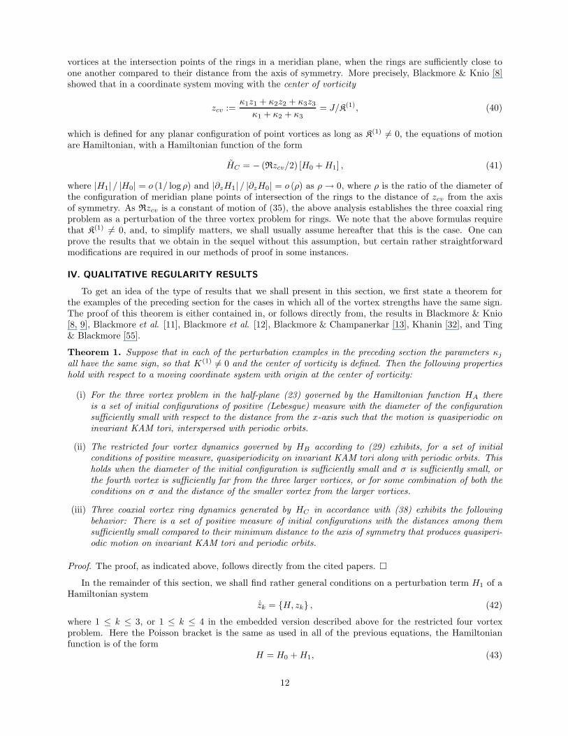
Elliptic case (K(2)> 0)

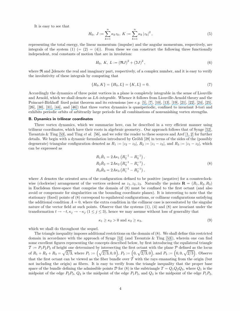
As indicated above, in the typical elliptic case, which is illustrated for T in Fig. 1, both the stationarypoint E and its (opposite orientation) copy E∗ are centers with index +1. It can be easily shown that thefixed points Q1, Q2 and Q3 are also centers. In addition, there are three other fixed points of (13) - one onthe interior of each side of T - denoted as Q4, Q5 and Q6 in Fig. 1, and each of these additional stationarypoints can readily be shown to be a saddle points of index −1. Notice that these observations are consistentwith the Poincare-Hopf Index theorem (see e.g. [31]) , inasmuch as a simple calculation yields

5(+1) + 3(−1) = 2 = χ (M) = χ (D(T )) ,

6

where χ(M) is the Euler-Poincare characteristic of the sphere M , which is two. In this case, we see thatthe global phase portrait of (15) is completely determined, and this leads to an exhaustive determinationof three vortex dynamics in the elliptic case owing to the unique integral path lifting principle mentionedabove.

..

Figure 1: Elliptic type with κ1 = 2, κ2 = 1, and κ3 = 1/2.

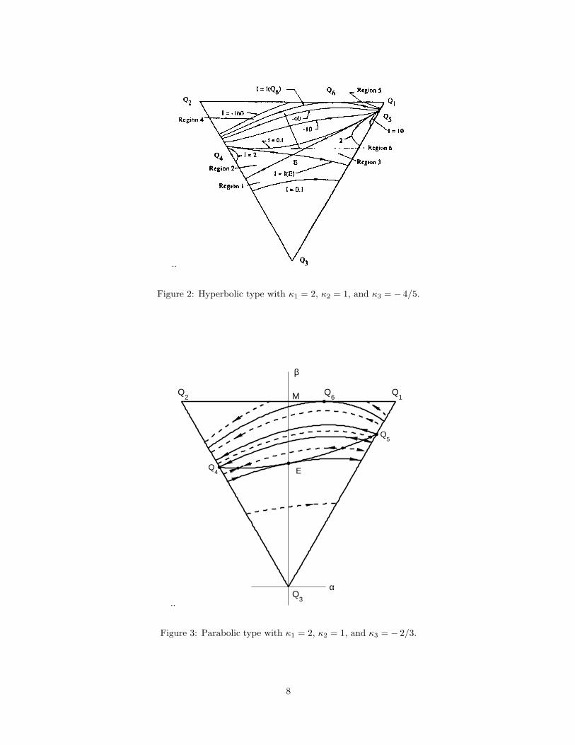
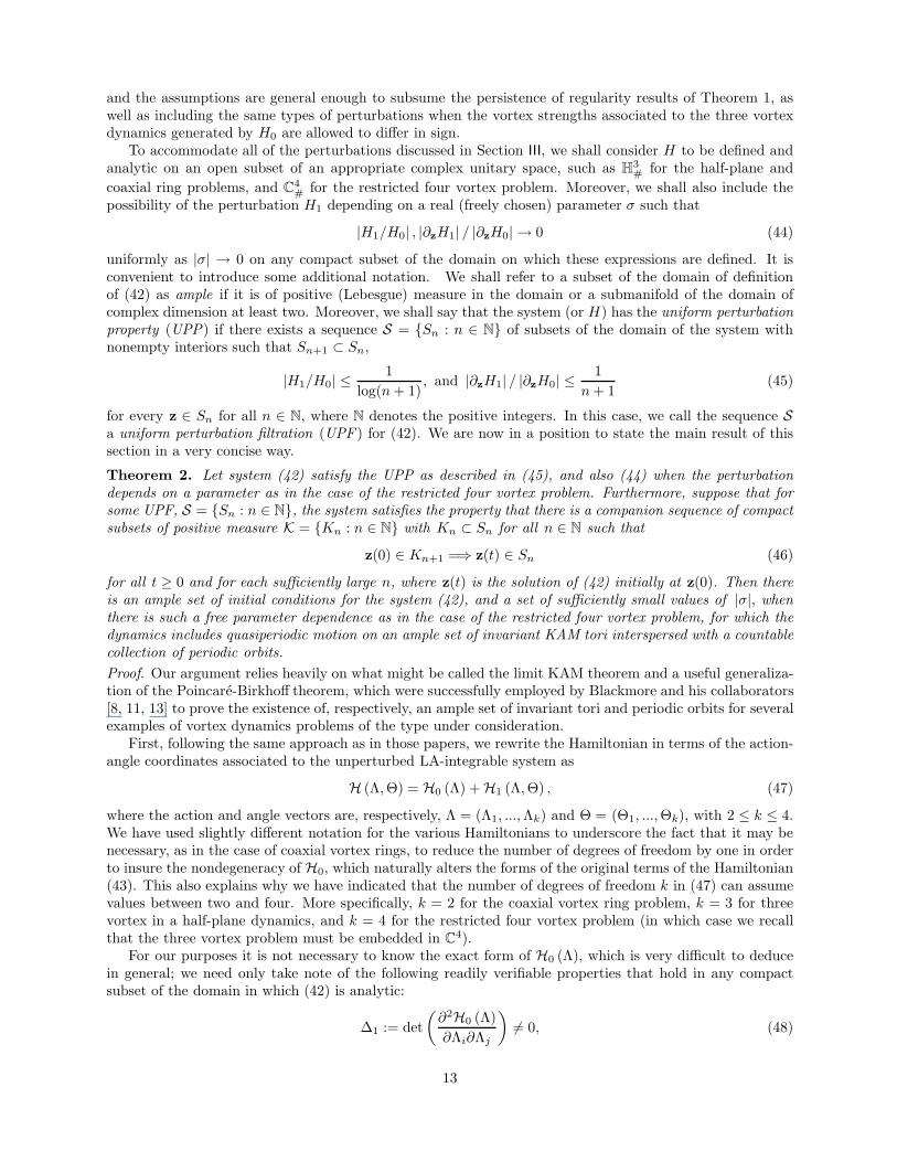
Hyperbolic case (K(2)< 0)

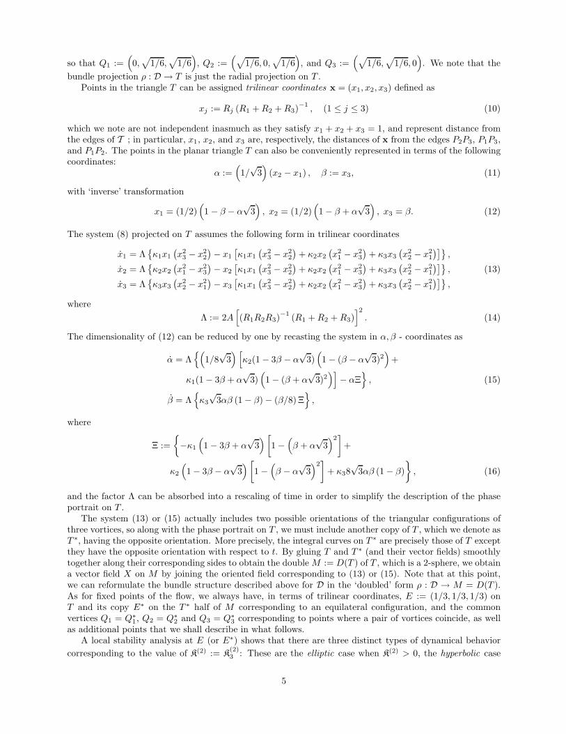
An example of the dynamics for the hyperbolic case is shown in Fig. 2. For all hyperbolic cases, thepoints E and E∗ associated to equilateral configurations are stationary saddle points of index −1. When itcomes to the fixed points at the vertices of the triangle T (glued to those of T ∗), the point Q3 is always acenter of index +1 for all possible admissible vortex strengths. Any other fixed points, which of course mustinclude the other vertices of T as well other points on the open edges of the triangle can have a variety ofnatures depending on certain algebraic criteria (see [53]). For example, in the case shown in Fig. 2, Q1 andQ2 are both centers, while the stationary points Q4, Q5 and Q6 are, respectively a center, center and saddlepoint. Thus we compute the following index sum

indE + indE∗ + indQ3 + indQ1 + indQ2 + indQ4 + indQ5 + indQ6 = 2(−1) + 5(+1) + (−1) = 2,

which is consistent with the Poincare-Hopf Index theorem.Depending on the algebraic criteria (involving the vortex strengths), there are exceptional cases where Q5

merges with Q1 or Q4 coincides with Q2, or possibly both, in which case one or both of Q1 and Q2 can assumethe form of a degenerate isolated stationary point of index +2. In all cases, the corresponding index sumcan be shown to be in agreement with the Poincare-Hopf formula. Exceptional cases notwithstanding, onceagain we also have, for any parameter values consistent with the hyperbolic case, a complete characterizationof three vortex dynamics owing to the unique integral path lifting principle.

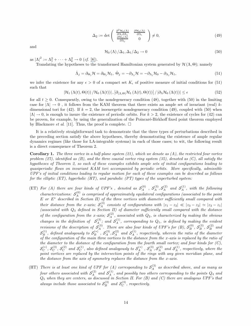
Parabolic case (K(2)= 0)

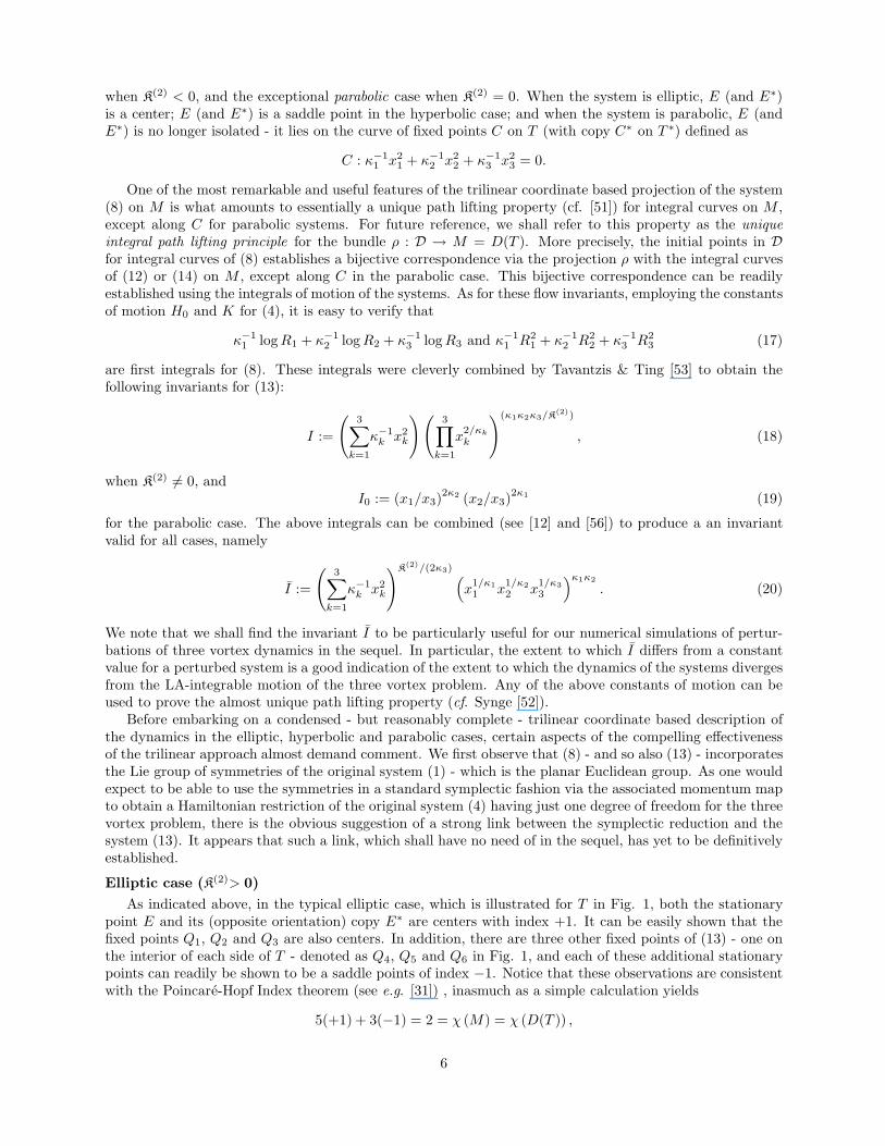
Three vortex dynamics represented in the trilinear coordinate phase plane for an example of the paraboliccase is illustrated in Fig. 3. Observe, as was discussed above, in this case the points E and E∗ lie on thesingular curve C in T and its copy C∗ on T ∗ comprised of stationary points of the system (13). Unfortunately,the unique integral path lifting principle does not apply on the double D (C) of C, which is a circle on Mto which the points E and E∗ both belong, and with this is associated another problem with the singularcurve exhibited in Fig. 3; namely, the trajectories of (13) appear to cross this curve, which is not what oneexpects for a reasonable dynamical system in which standard uniqueness theorems obtain. But the principledoes apply on the complement of D (C) on M , making it possible to obtain an almost complete descriptionof three vortex dynamics in the parabolic case. To fill in the gaps, it is necessary only to conduct a more

7

..

Figure 2: Hyperbolic type with κ1 = 2, κ2 = 1, and κ3 = − 4/5.

..

α

β

Q1

Q2

Q3

M

E

Q5

Q4

Q6

Figure 3: Parabolic type with κ1 = 2, κ2 = 1, and κ3 = − 2/3.

8

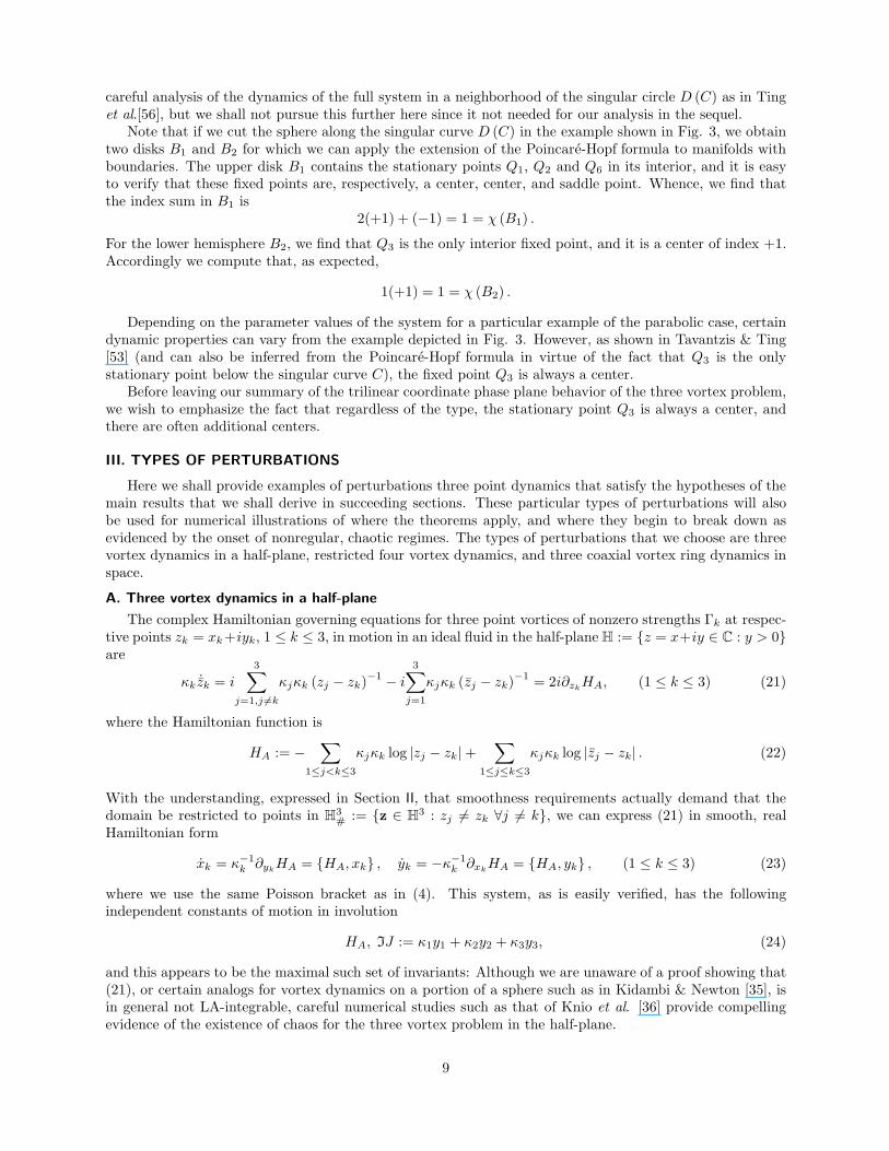
careful analysis of the dynamics of the full system in a neighborhood of the singular circle D (C) as in Tinget al.[56], but we shall not pursue this further here since it not needed for our analysis in the sequel.

Note that if we cut the sphere along the singular curve D (C) in the example shown in Fig. 3, we obtaintwo disks B1 and B2 for which we can apply the extension of the Poincare-Hopf formula to manifolds withboundaries. The upper disk B1 contains the stationary points Q1, Q2 and Q6 in its interior, and it is easyto verify that these fixed points are, respectively, a center, center, and saddle point. Whence, we find thatthe index sum in B1 is

2(+1) + (−1) = 1 = χ (B1) .

For the lower hemisphere B2, we find that Q3 is the only interior fixed point, and it is a center of index +1.Accordingly we compute that, as expected,

1(+1) = 1 = χ (B2) .

Depending on the parameter values of the system for a particular example of the parabolic case, certaindynamic properties can vary from the example depicted in Fig. 3. However, as shown in Tavantzis & Ting[53] (and can also be inferred from the Poincare-Hopf formula in virtue of the fact that Q3 is the onlystationary point below the singular curve C), the fixed point Q3 is always a center.

Before leaving our summary of the trilinear coordinate phase plane behavior of the three vortex problem,we wish to emphasize the fact that regardless of the type, the stationary point Q3 is always a center, andthere are often additional centers.

III. TYPES OF PERTURBATIONS

Here we shall provide examples of perturbations three point dynamics that satisfy the hypotheses of themain results that we shall derive in succeeding sections. These particular types of perturbations will alsobe used for numerical illustrations of where the theorems apply, and where they begin to break down asevidenced by the onset of nonregular, chaotic regimes. The types of perturbations that we choose are threevortex dynamics in a half-plane, restricted four vortex dynamics, and three coaxial vortex ring dynamics inspace.

A. Three vortex dynamics in a half-plane

The complex Hamiltonian governing equations for three point vortices of nonzero strengths Γk at respec-tive points zk = xk+iyk, 1 ≤ k ≤ 3, in motion in an ideal fluid in the half-plane H := {z = x+iy ∈ C : y > 0}are

κk ˙zk = i3∑

j=1,j 6=k

κjκk (zj − zk)−1 − i3∑

j=1

κjκk (zj − zk)−1 = 2i∂zkHA, (1 ≤ k ≤ 3) (21)

where the Hamiltonian function is

HA := −∑

1≤j<k≤3

κjκk log |zj − zk| +∑

1≤j≤k≤3

κjκk log |zj − zk| . (22)

With the understanding, expressed in Section II, that smoothness requirements actually demand that thedomain be restricted to points in H3

# := {z ∈ H3 : zj 6= zk ∀j 6= k}, we can express (21) in smooth, realHamiltonian form

xk = κ−1k ∂yk

HA = {HA, xk} , yk = −κ−1k ∂xk

HA = {HA, yk} , (1 ≤ k ≤ 3) (23)

where we use the same Poisson bracket as in (4). This system, as is easily verified, has the followingindependent constants of motion in involution

HA, IJ := κ1y1 + κ2y2 + κ3y3, (24)

and this appears to be the maximal such set of invariants: Although we are unaware of a proof showing that(21), or certain analogs for vortex dynamics on a portion of a sphere such as in Kidambi & Newton [35], isin general not LA-integrable, careful numerical studies such as that of Knio et al. [36] provide compellingevidence of the existence of chaos for the three vortex problem in the half-plane.

9

From a perturbation perspective, we can obviously write the Hamiltonian function in the form

HA = H0 + HA,1, (25)

whereHA,1 :=

∑

1≤j≤k≤3

κjκk log |zj − zk| . (26)

Now it is obvious from the nature of these various functions that there exist extensive regions in H# at anypositive distance away from the boundary (the x-axis) where we have both |Ha| ≪ |H0| and |∂zHa| ≪ |∂zH0|,in keeping with our point of view of treating (21) as a (small) perturbation of three vortex dynamics.

B. Restricted four vortex dynamics

By the restricted four vortex problem (dynamics), we mean the motion of four point vortices in an idealfluid in the (complex) plane C (= R2), where three of the vortices, located at points z1, z2 and z3, haverespective nonzero strengths Γ1, Γ2 and Γ3, while the fourth vortex at the point z4 has strength Γ4 satisfying|Γ4| ≪ m := min{|Γ1| , |Γ2| , |Γ3|} and we have the freedom of making |Γ4| /m as small as we wish. It followsfrom (4) that the complex Hamiltonian governing equations are

κk ˙zk = i

4∑

j=1,j 6=k

κjκk (zj − zk)−1

= 2i∂zkHB , (1 ≤ k ≤ 4) (27)

where the Hamiltonian function is

HB := −∑

1≤j<k≤4

κjκk log |zj − zk| . (28)

Of course this can be put into the following real Hamiltonian form using the same Poisson brackets as in (4):

xk = κ−1k ∂yk

HB = {HB, xk} , yk = −κ−1k ∂xk

HB = {HB, yk} , (1 ≤ k ≤ 4) (29)

where analogous adjustments in the domain are obviously required to insure smoothness. Just as in the caseof (4), symmetry considerations show that (26) has the motion invariants

HB, J :=

4∑

k=1

κkzk, K :=

4∑

k=1

κk |zk|2 , (30)

with the following independent integrals in involution

HB, K, L := (RJ)2+ (IJ)

2. (31)

These three independent integrals in involution represent the maximal number, as it has been proved thatthe system (29) is not integrable in general (see Bagrets & Bagrets [6] and Ziglin [58]). We note, however,that there are certain special cases of four vortex motion on a plane or sphere that are LA-integrable, asshown in Aref & Stremler [3], Borisov et al. [17], Eckhardt [23], Sakajo [49], and Sokolovskiy & Verron [50].

Our focus here is to treat (27) or (29) as a perturbation of the three vortex problem. To be mathematicallyprecise, we actually have to consider the system as a perturbation of the three vortex problem embedded inC4, by which we mean

κk ˙zk = i

3∑

j=1,j 6=k

κjκk (zj − zk)−1

= 2i∂zkH0, (1 ≤ k ≤ 3)

˙z4 = 0 = 2i∂z4H0. (32)

Obviously this embedded system is also LA-integrable, and its dynamics consists of a two-parameter infinityof copies of three vortex dynamics - one for each constant value of z4. This having been said, there is noharm in the slight abuse of notation that we shall use from now on of treating the restricted four vortex

10

problem as a perturbation of the three vortex problem. To highlight the perturbation aspect, we write theHamiltonian function in the form

HB = H0 + HB,1, (33)

where

HB,1 := −σ

3∑

j=1

κj log |zj − z4| , (34)

and we have replaced κ4 by σ to emphasize the fact that this parameter may be chosen to be as small asnecessary to insure the desired perturbation behavior.

C. Three slender coaxial vortex ring dynamics

Consider three (circular) coaxial vortex rings of respective nonzero strengths Γ1, Γ2 and Γ3, with axisof symmetry the y-axis, in motion in an ideal fluid in R3. The rings intersect any meridian half-planebounded along the y-axis in unique points (r1, y1), (r2, y2) and (r3, y3), respectively, where r is the distancefrom the y-axis, and the motion of the rings is completely determined by these points owing to the axialsymmetry of the equations of motion. It is convenient to set z := r2 + iy = s + iy, so that the motion ofthe three intersection points can be considered to be in the half-plane H. The complex Hamiltonian form ofthe dynamical equation of motion of these points - de-singularized in a standard way to eliminate the usualinfinity in the self-induced velocity of the rings -can be expressed as (cf. Blackmore & Knio [8, 9], Blackmoreet al. [11], and Lamb [38])

κk ˙zk =3∑

j=1,j 6=k

κjκkrjrk (zj − zk)

∫ π/2

0

∆−3/2jk cos 2αdα − iκ2

kr−1k

[

log(

8rkδ−1c

)

− 0.558]

− 2i3∑

j=1,j 6=k

κjκkrj

∫ π/2

0

(rj − rk cos 2α)∆−3/2jk dα (35)

= 2i∂zkHC , (1 ≤ k ≤ 3)

where δc is a very small positive number representing the common core radii (used in the de-singularizationprocedure) of the vortex rings,

∆jk := (rk − rj)2

+ (yk − yj)2

+ 4rjrk sin2 α, (36)

and the Hamiltonian function is

HC := −23∑

j=1

κ2jrj

[

log(

8rjδ−1c

)

− 1.558]

− 4∑

1≤j<k≤3

κjκkrjrk

∫ π/2

0

∆−1/2jk cos 2αdα. (37)

This system can, employing the same Poisson bracket used in (4), be recast in the real Hamiltonian form

sk = κ−1k ∂yk

HC = {HC , sk} , yk = −κ−1k ∂sk

HC = {HC , yk} . (1 ≤ k ≤ 3) (38)

It is easy to show that (37) has the two following independent integrals in involution

HC , G :=

3∑

j=1

κjsj =

3∑

j=1

κjr2j . (39)

However, there are no additional independent invariants in involution, as proved in Bagrets & Bagrets [6], soalthough the dynamics of two coaxial rings is LA-integrable, this is not true in general for the system (35)or (38).

The formulation of (35) as a perturbation of three vortex dynamics is rather more subtle than that of thetwo preceding examples. Formulas obtained by Callegari & Ting [18] indicate that, relative to a coordinatesystem moving along the axis of symmetry with the overall translation velocity of the ring configuration, theequations of motion of the rings are closely approximated (modulo a constant factor) by those of three point

11

vortices at the intersection points of the rings in a meridian plane, when the rings are sufficiently close toone another compared to their distance from the axis of symmetry. More precisely, Blackmore & Knio [8]showed that in a coordinate system moving with the center of vorticity

zcv :=κ1z1 + κ2z2 + κ3z3

κ1 + κ2 + κ3= J/K(1), (40)

which is defined for any planar configuration of point vortices as long as K(1) 6= 0, the equations of motionare Hamiltonian, with a Hamiltonian function of the form

HC = − (Rzcv/2) [H0 + H1] , (41)

where |H1| / |H0| = o (1/ log ρ) and |∂zH1| / |∂zH0| = o (ρ) as ρ → 0, where ρ is the ratio of the diameter ofthe configuration of meridian plane points of intersection of the rings to the distance of zcv from the axisof symmetry. As Rzcv is a constant of motion of (35), the above analysis establishes the three coaxial ringproblem as a perturbation of the three vortex problem for rings. We note that the above formulas requirethat K(1) 6= 0, and, to simplify matters, we shall usually assume hereafter that this is the case. One canprove the results that we obtain in the sequel without this assumption, but certain rather straightforwardmodifications are required in our methods of proof in some instances.

IV. QUALITATIVE REGULARITY RESULTS

To get an idea of the type of results that we shall present in this section, we first state a theorem forthe examples of the preceding section for the cases in which all of the vortex strengths have the same sign.The proof of this theorem is either contained in, or follows directly from, the results in Blackmore & Knio[8, 9], Blackmore et al. [11], Blackmore et al. [12], Blackmore & Champanerkar [13], Khanin [32], and Ting& Blackmore [55].

Theorem 1. Suppose that in each of the perturbation examples in the preceding section the parameters κj

all have the same sign, so that K(1) 6= 0 and the center of vorticity is defined. Then the following propertieshold with respect to a moving coordinate system with origin at the center of vorticity:

(i) For the three vortex problem in the half-plane (23) governed by the Hamiltonian function HA thereis a set of initial configurations of positive (Lebesgue) measure with the diameter of the configurationsufficiently small with respect to the distance from the x-axis such that the motion is quasiperiodic oninvariant KAM tori, interspersed with periodic orbits.

(ii) The restricted four vortex dynamics governed by HB according to (29) exhibits, for a set of initialconditions of positive measure, quasiperiodicity on invariant KAM tori along with periodic orbits. Thisholds when the diameter of the initial configuration is sufficiently small and σ is sufficiently small, orthe fourth vortex is sufficiently far from the three larger vortices, or for some combination of both theconditions on σ and the distance of the smaller vortex from the larger vortices.

(iii) Three coaxial vortex ring dynamics generated by HC in accordance with (38) exhibits the followingbehavior: There is a set of positive measure of initial configurations with the distances among themsufficiently small compared to their minimum distance to the axis of symmetry that produces quasiperi-odic motion on invariant KAM tori and periodic orbits.

Proof. The proof, as indicated above, follows directly from the cited papers. �

In the remainder of this section, we shall find rather general conditions on a perturbation term H1 of aHamiltonian system

˙zk = {H, zk} , (42)

where 1 ≤ k ≤ 3, or 1 ≤ k ≤ 4 in the embedded version described above for the restricted four vortexproblem. Here the Poisson bracket is the same as used in all of the previous equations, the Hamiltonianfunction is of the form

H = H0 + H1, (43)

12

and the assumptions are general enough to subsume the persistence of regularity results of Theorem 1, aswell as including the same types of perturbations when the vortex strengths associated to the three vortexdynamics generated by H0 are allowed to differ in sign.

To accommodate all of the perturbations discussed in Section III, we shall consider H to be defined andanalytic on an open subset of an appropriate complex unitary space, such as H

3# for the half-plane and

coaxial ring problems, and C4# for the restricted four vortex problem. Moreover, we shall also include the

possibility of the perturbation H1 depending on a real (freely chosen) parameter σ such that

|H1/H0| , |∂zH1| / |∂zH0| → 0 (44)

uniformly as |σ| → 0 on any compact subset of the domain on which these expressions are defined. It isconvenient to introduce some additional notation. We shall refer to a subset of the domain of definitionof (42) as ample if it is of positive (Lebesgue) measure in the domain or a submanifold of the domain ofcomplex dimension at least two. Moreover, we shall say that the system (or H) has the uniform perturbationproperty (UPP) if there exists a sequence S = {Sn : n ∈ N} of subsets of the domain of the system withnonempty interiors such that Sn+1 ⊂ Sn,

|H1/H0| ≤1

log(n + 1), and |∂zH1| / |∂zH0| ≤

1

n + 1(45)

for every z ∈ Sn for all n ∈ N, where N denotes the positive integers. In this case, we call the sequence Sa uniform perturbation filtration (UPF ) for (42). We are now in a position to state the main result of thissection in a very concise way.

Theorem 2. Let system (42) satisfy the UPP as described in (45), and also (44) when the perturbationdepends on a parameter as in the case of the restricted four vortex problem. Furthermore, suppose that forsome UPF, S = {Sn : n ∈ N}, the system satisfies the property that there is a companion sequence of compactsubsets of positive measure K = {Kn : n ∈ N} with Kn ⊂ Sn for all n ∈ N such that

z(0) ∈ Kn+1 =⇒ z(t) ∈ Sn (46)

for all t ≥ 0 and for each sufficiently large n, where z(t) is the solution of (42) initially at z(0). Then thereis an ample set of initial conditions for the system (42), and a set of sufficiently small values of |σ|, whenthere is such a free parameter dependence as in the case of the restricted four vortex problem, for which thedynamics includes quasiperiodic motion on an ample set of invariant KAM tori interspersed with a countablecollection of periodic orbits.

Proof. Our argument relies heavily on what might be called the limit KAM theorem and a useful generaliza-tion of the Poincare-Birkhoff theorem, which were successfully employed by Blackmore and his collaborators[8, 11, 13] to prove the existence of, respectively, an ample set of invariant tori and periodic orbits for severalexamples of vortex dynamics problems of the type under consideration.

First, following the same approach as in those papers, we rewrite the Hamiltonian in terms of the action-angle coordinates associated to the unperturbed LA-integrable system as

H (Λ, Θ) = H0 (Λ) + H1 (Λ, Θ) , (47)

where the action and angle vectors are, respectively, Λ = (Λ1, ..., Λk) and Θ = (Θ1, ..., Θk), with 2 ≤ k ≤ 4.We have used slightly different notation for the various Hamiltonians to underscore the fact that it may benecessary, as in the case of coaxial vortex rings, to reduce the number of degrees of freedom by one in orderto insure the nondegeneracy of H0, which naturally alters the forms of the original terms of the Hamiltonian(43). This also explains why we have indicated that the number of degrees of freedom k in (47) can assumevalues between two and four. More specifically, k = 2 for the coaxial vortex ring problem, k = 3 for threevortex in a half-plane dynamics, and k = 4 for the restricted four vortex problem (in which case we recallthat the three vortex problem must be embedded in C

4).For our purposes it is not necessary to know the exact form of H0 (Λ), which is very difficult to deduce

in general; we need only take note of the following readily verifiable properties that hold in any compactsubset of the domain in which (42) is analytic:

∆1 := det

(

∂2H0 (Λ)

∂Λi∂Λj

)

6= 0, (48)

13

∆2 := det

(

∂2H0(Λ)∂Λi∂Λj

∂H0(Λ)∂Λi

∂H0(Λ)∂Λj

0

)

6= 0, (49)

andH0 (Λ) /∆1, ∆1/∆2 → 0 (50)

as |Λ|2 := Λ21 + · · · + Λ2

k → 0 (cf. [8]).Translating the hypotheses to the transformed Hamiltonian system generated by H (Λ, Θ); namely

Λj = ∂ΘjH = ∂Θj

H1, Θj = −∂ΛjH = −∂Λj

H0 − ∂ΛjH1, (51)

we infer the existence for any ǫ > 0 of a compact set Kǫ of positive measure of initial conditions for (51)such that

|H1 (Λ(t), Θ(t)) /H0 (Λ(t))| ,∣

∣∂(Λ,Θ)H1 (Λ(t), Θ(t))∣

∣ / |∂ΛH0 (Λ(t))| ≤ ǫ (52)

for all t ≥ 0. Consequently, owing to the nondegeneracy condition (48), together with (50) in the limitingcase for |Λ| → 0 , it follows from the KAM theorem that there exists an ample set of invariant (real) k-dimensional tori for (42). If k = 2, the isoenergetic nondegeneracy condition (49), coupled with (50) when|Λ| → 0, is enough to insure the existence of periodic orbits. For k > 2, the existence of cycles for (42) canbe proven, for example, by using the generalization of the Poincare-Birkhoff fixed point theorem employedby Blackmore et al. [11]. Thus, the proof is complete. �

It is a relatively straightforward task to demonstrate that the three types of perturbations described inthe preceding section satisfy the above hypotheses, thereby demonstrating the existence of ample regulardynamics regimes (like those for LA-integrable systems) in each of those cases; to wit, the following resultis a direct consequence of Theorem 2.

Corollary 1. The three vortex in a half-plane system (21), which we denote as (A), the restricted four vortexproblem (27), identified as (B), and the three coaxial vortex ring system (35), denoted as (C), all satisfy thehypotheses of Theorem 2, so each of these examples exhibits ample sets of initial configurations leading toquasiperiodic flows on invariant KAM tori accompanied by periodic orbits. More specifically, admissibleUPF’s of initial conditions leading to regular motion for each of these examples can be described as followsfor the elliptic (ET), hyperbolic (HT), and parabolic (PT) types of the unperturbed system:

(ET) For (A) there are four kinds of UPF’s , denoted as S(0)A , S(3)

A ,S(2)A and S(1)

A , with the following

characterizations: S(0)A is comprised of approximately equilateral configurations (associated to the point

E or E∗ described in Section II) of the three vortices with diameter sufficiently small compared with

their distance from the x-axis; S(3)A consists of configurations with |z1 − z2| ≪ |z3 − z2| ≃ |z3 − z1|

(associated with Q3 defined in Section II) of diameter sufficiently small compared with the distance

of the configuration from the x-axis; S(2)A , associated with Q2, is characterized by making the obvious

changes in the definition of S(3)A ; and S(1)

A , corresponding to Q1, is defined by making the evident

revisions of the description of S(3)A . There are also four kinds of UPF’s for (B), S(0)

B , S(3)B , S(2)

B and

S(1)B , defined analogously to S(∗)

B , S(3)A ,S(2)

A and S(1)A , respectively, wherein the ratio of the diameter

of the configuration of the main three vortices to the distance from the x-axis is replaced by the ratio ofthe diameter to the distance of the configuration from the fourth small vortex; and four kinds for (C),

S(∗)C , S(3)

C , S(2)C and S(1)

C , also defined analogously to S(∗)A , S(3)

A ,S(2)A and S(1)

A , respectively, where thepoint vortices are replaced by the intersection points of the rings with any given meridian plane, andthe distance from the axis of symmetry replaces the distance from the x-axis.

(HT) There is at least one kind of UPF for (A) corresponding to S(3)A as described above, and as many as

four others associated with S(2)A and S(1)

A , and possibly two others corresponding to the points Q4 andQ5 when they are centers, as discussed in Section II. For (B) and (C) there are analogous UPF’s that

always include those associated to S(3)B and S(3)

C , respectively.

14

(PT) For (A), (B) and (C) there is always one UPF corresponding to S(3)A , S(3)

B and S(3)C , respectively, and

possibly additional UPF associated to any other possible centers as described in the trilinear phase planecharacterization of the dynamics covered in Section II.

Proof. We shall provide detailed arguments only for the three vortex system in the half-plane, either whenthe strengths of all vortices have the same sign (the elliptic type), or they differ in sign (which includes boththe hyperbolic and parabolic types). The verifications for the restricted four vortex, and three coaxial vortexring problems for the various types of the unperturbed (three vortex) system can be obtained analogously bystraightforward - but rather lengthy - calculations, and we shall leave the details to the reader, noting thatthe desired results when the unperturbed system is of elliptic type actually follow directly from Theorem 1.

Even though, as mentioned above, the conclusions we are seeking are a direct consequence of Theorem1 when the unperturbed system is of elliptic type, we shall include a proof here, since it will be helpful inpointing the way to establishing sufficient conditions for the hyperbolic and parabolic types. Recalling thatthere is no loss of generality in assuming that κ1 ≥ κ2 ≥ κ3 > 0 when the unperturbed system is elliptic, wefirst rewrite the constants of motion (24) of (23) in a form more useful to our purposes; namely

HA = c1 = κ21 log (2y1) + κ2

2 log (2y2) + κ23 log (2y3) − κ1κ2 log

[

(x1 − x2)2 + (y1 − y2)

2

(x1 − x2)2 + (y1 + y2)2

]1/2

−

κ1κ3 log

[

(x1 − x3)2 + (y1 − y3)

2

(x1 − x3)2 + (y1 + y3)2

]1/2

− κ2κ3 log

[

(x2 − x3)2 + (y2 − y3)

2

(x2 − x3)2 + (y2 + y3)2

]1/2

, (53)

IJ = c2 = κ1y1 + κ2y2 + κ3y3,

and define M (c1, c2) to be the set of points in H3# satisfying the pair of equations (53).

It is straightforward to show directly from the form of these defining equations that given any arbitrarilylarge and small positive number, respectively, λ and ν, there exist λ∗ = λ∗(λ, ν) ≥ λ and 0 < ν∗ = ν∗(λ, ν) <ν such that the following property is satisfied if c1 and c2 are chosen to be sufficiently large positive numbers:let the initial positions of the vortices, z1(0) = x1(0)+iy1(0), z2(0) = x2(0)+iy2(0), z3(0) = x3(0)+iy3(0) beapproximately in the shape of an equilateral triangle (corresponding to E in Fig.1) of diameter less than ν∗,with y1(0), y2(0), y3(0) ≥ λ∗, and define M∗ (c1, c2) to be the component of M (c1, c2) containing the initialpoint z(0). Then for all configurations (z1, z2, z3) in the component M∗ (c1, c2), the diameter is less than orequal to ν, and y1, y2, y3 ≥ λ. Owing to the connectedness of orbits of (23), it must therefore follow that thediameter of the configuration z(t) = (z1(t), z2(t), z3(t)) is less than or equal to ν, and y1(t), y2(t), y3(t) ≥ λfor all t ≥ 0, where z(t) is the solution of (23) with the specified initial condition. Whence the constructionof the desired UPF associated to these sets is a simple matter.

If the unperturbed system is hyperbolic or parabolic, then as indicated in Section II, we may - and do -assume without loss of generality that κ1 ≥ κ2 > 0 > κ3. This puts a slightly different complexion on thesystem of equations (53), which must be satisfied by all solutions of (23). However, not so different thatwe cannot use the same kind of argument as for the elliptic type system (given above) modulo a few ratherobvious modifications. In fact, we can take our cue for the necessary adjustments by recalling our discussionof the trilinear phase portraits for the three vortex problem in Section II. It is not difficult to see from aclose inspection of (53) for the case when κ3 is negative - in which we concentrate on those terms containingthe negative vortex strength - that we can simply change the initial condition on the vortex configurationto conform to the center Q3 (see Figs 1 and 2). More precisely, we need only change the description of theinitial configuration in the preceding paragraph so that |z1(0) − z2(0)| ≪ |z1(0) − z3(0)| ≃ |z2(0) − z3(0)|in order to obtain orbits of (23) staying in a component of M (c1, c2) analogous to M∗ (c1, c2). Just as inthe previous paragraph, this leads directly to the desired UPF’s for the hyperbolic and parabolic cases, andcompletes the proof for three vortex dynamics in the half-plane. �

Before moving on to a study of perturbations of specific periodic orbits of three vortex dynamics, we notethat the following generalization of Theorem 2 can be easily proved by using essentially the same argumentsas in its proof given above.

Theorem 3. Suppose the system (42) is a perturbation of a general LA-integrable Hamiltonian systemgenerated by H0, and that H is defined and analytic on an open subset of Cm, with m ≥ 1. In addition,

15

assume that (42) satisfies the hypotheses of Theorem 2, and that the usual KAM nondegeneracy conditionholds for H0 in an admissible UPF. Then there exists an ample set of initial conditions (and small values of aparameter, if pertinent) such that the system exhibits quasiperiodic flows on an ample collection of invarianttori, together with periodic orbits.

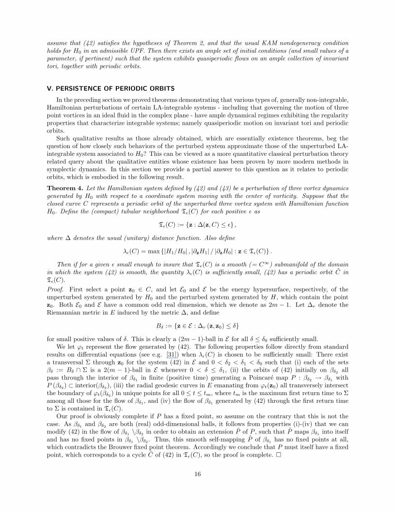
V. PERSISTENCE OF PERIODIC ORBITS

In the preceding section we proved theorems demonstrating that various types of, generally non-integrable,Hamiltonian perturbations of certain LA-integrable systems - including that governing the motion of threepoint vortices in an ideal fluid in the complex plane - have ample dynamical regimes exhibiting the regularityproperties that characterize integrable systems; namely quasiperiodic motion on invariant tori and periodicorbits.

Such qualitative results as those already obtained, which are essentially existence theorems, beg thequestion of how closely such behaviors of the perturbed system approximate those of the unperturbed LA-integrable system associated to H0? This can be viewed as a more quantitative classical perturbation theoryrelated query about the qualitative entities whose existence has been proven by more modern methods insymplectic dynamics. In this section we provide a partial answer to this question as it relates to periodicorbits, which is embodied in the following result.

Theorem 4. Let the Hamiltonian system defined by (42) and (43) be a perturbation of three vortex dynamicsgenerated by H0 with respect to a coordinate system moving with the center of vorticity. Suppose that theclosed curve C represents a periodic orbit of the unperturbed three vortex system with Hamiltonian functionH0. Define the (compact) tubular neighborhood Tǫ(C) for each positive ǫ as

Tǫ(C) := {z : ∆(z, C) ≤ ǫ} ,

where ∆ denotes the usual (unitary) distance function. Also define

λǫ(C) = max {|H1/H0| , |∂zH1| / |∂zH0| : z ∈ Tǫ(C)} .

Then if for a given ǫ small enough to insure that Tǫ(C) is a smooth (= C∞) submanifold of the domainin which the system (42) is smooth, the quantity λǫ(C) is sufficiently small, (42) has a periodic orbit C inTǫ(C).

Proof. First select a point z0 ∈ C, and let E0 and E be the energy hypersurface, respectively, of theunperturbed system generated by H0 and the perturbed system generated by H , which contain the pointz0. Both E0 and E have a common odd real dimension, which we denote as 2m − 1. Let ∆r denote theRiemannian metric in E induced by the metric ∆, and define

Bδ := {z ∈ E : ∆r (z, z0) ≤ δ}

for small positive values of δ. This is clearly a (2m − 1)-ball in E for all δ ≤ δ0 sufficiently small.We let ϕt represent the flow generated by (42). The following properties follow directly from standard

results on differential equations (see e.g. [31]) when λǫ(C) is chosen to be sufficiently small: There exista transversal Σ through z0 for the system (42) in E and 0 < δ2 < δ1 < δ0 such that (i) each of the setsβδ := Bδ ∩ Σ is a 2(m − 1)-ball in E whenever 0 < δ ≤ δ1, (ii) the orbits of (42) initially on βδ2 allpass through the interior of βδ1 in finite (positive time) generating a Poincare map P : βδ2 → βδ1 withP (βδ2) ⊂ interior(βδ2), (iii) the radial geodesic curves in E emanating from ϕt(z0) all transversely intersectthe boundary of ϕt(βδ2) in unique points for all 0 ≤ t ≤ tm, where tm is the maximum first return time to Σamong all those for the flow of βδ1 , and (iv) the flow of βδ1 generated by (42) through the first return timeto Σ is contained in Tǫ(C).

Our proof is obviously complete if P has a fixed point, so assume on the contrary that this is not thecase. As βδ1 and βδ2 are both (real) odd-dimensional balls, it follows from properties (i)-(iv) that we canmodify (42) in the flow of βδ1 \βδ2 in order to obtain an extension P of P , such that P maps βδ1 into itselfand has no fixed points in βδ1 \βδ2 . Thus, this smooth self-mapping P of βδ1 has no fixed points at all,which contradicts the Brouwer fixed point theorem. Accordingly we conclude that P must itself have a fixedpoint, which corresponds to a cycle C of (42) in Tǫ(C), so the proof is complete. �

16

Considering the generality of the above result, and the relative simplicity of the proof, it seems as thoughthis should have certainly been discovered. However, the authors were unable to find such a result in theliterature, although it appears that it could be derived rather directly from certain results that prove theexistence of periodic solutions for Hamiltonian systems employing index theory (cf. Blackmore & Wang [10],Gole [26] and Josellis [30]). It is interesting to take note of the very special case where ∂zH1 in the abovetheorem takes the form ∂zH1 = φ(z)∂zH0, where φ is a smooth, real valued function whose magnitude canbe made arbitrarily small in the tubular neighborhood Tǫ(C). Then as one can readily see by making theobvious transformation of the time parameter, the cycle of the perturbed system is not just an approximationof C, it is identical with it, and the local flow of the perturbed system is identical with that of the unperturbedsystem (modulo a change of parametrization).

Theorem 4 can be applied directly to the perturbations of three vortex dynamics that we have beenconsidering to identify conditions under which the perturbation has a periodic orbit close to one for thethree vortex problem. We leave the very straightforward proof of the next result to the reader.

Corollary 2. The hypothesis and conclusions of Theorem 4 regarding the existence of a periodic orbit of theperturbed system close to a periodic orbit C : z = z(t), 0 ≤ t ≤ p, of the unperturbed (three vortex) systemhold for (A) three vortices in a half-plane, (B) restricted four vortex dynamics, and (C) three slender coaxialring dynamics obtain under the following conditions:

(a) Each of the coordinates of z(t) on C is sufficiently distant from the x-axis in the complex plane.

(b) For the coordinates z(t) = (z1(t), z2(t), z3(t), z4(t)) ∈ C, the distance in the complex plane C fromz4(0) to the set {z ∈ C : z = z1(t), z2(t) or z3(t), 0 ≤ t ≤ p} is sufficiently large, or the magnitudeof the strength of the fourth vortex is sufficiently small, or a suitable combination of both of theseconditions is enforced.

(c) The coordinates of z(t) on C representing the points of intersection of the rings with a meridian planeare sufficiently far from the axis of symmetry (represented by the y-axis in this plane).

We note that the conditions given in Corollary 2 by no means exhaust all possible situations where theperturbed system has a periodic orbit close to a periodic orbit of the unperturbed system. For example, it iseasy to see that in the restricted four vortex problem there are many such cases where the fourth small vortexis neither particularly small nor very distant from the three large vortices: Simply consider any configurationof the large vortices that generates a periodic solution of the three vortex problem, and place the fourthvortex, of any strength, at the center of vorticity of the larger vortices. Then the fourth vortex remainsfixed, and the motion of the three larger vortices is unaffected by its presence.

VI. SIMULATIONS OF DYNAMICS

In this section we provide numerical examples that illustrate the persistence of regular motion for differenttypes of perturbations, as well as breakdown of regularity as large perturbations are considered and thehypotheses of our theoretical results are accordingly violated. As mentioned earlier, we consider half-planedynamics, restricted four vortex perturbations, and slender coaxial vortex ring dynamics , which we refer tobelow as type A, B, and C, respectively.

Our simulations cover just a small sample of possible cases for the various perturbations, and they arepresented in two basic types of graphical forms: As trajectories in the plane or half-plane, or as Poincaresections, which are especially well suited to illuminating transitions from regular to chaotic motion. Inparticular, for the unperturbed system we present plots of the trajectories of the three vortices in the plane,juxtaposed with the corresponding trilinear phase plane stationary point. If any of the perturbation typessatisfy the hypotheses of Corollaries 1 and 2, we expect that plots of the trajectories of their vortex elements(with respect to a coordinate system moving with the configuration) would show a small variation of theplots for the unperturbed system. Also included for type A perturbations are Poincare maps, along withthe corresponding Poincare map for the unperturbed system, showing that there is a transition to chaoticmotion as the array starts closer to the boundary of the half-plane compared to the diameter of the initialconfiguration of vortices. For type C perturbations, we present Poincare maps exhibiting strong regularitywhen the slender coaxial rings are very close to one another compared to the distance of the configuration

17

from the axis of symmetry, as expected in view of Corollary 1. For the restricted four vortex problem, apair of Poincare maps shows how the motion tends to be more chaotic as the initial position and strengthof the fourth small vortex, respectively, starts closer to the initial group of three larger vortices and growsin comparison to the strengths of this group. This behavior is entirely consistent with Corollaries 1 and 2.

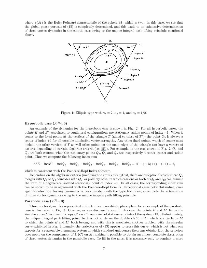
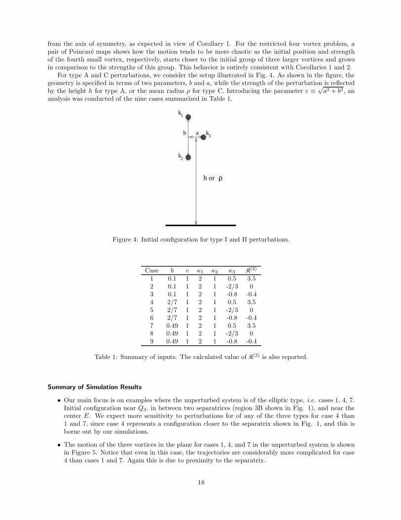
For type A and C perturbations, we consider the setup illustrated in Fig. 4. As shown in the figure, thegeometry is specified in terms of two parameters, b and a, while the strength of the perturbation is reflectedby the height h for type A, or the mean radius ρ for type C. Introducing the parameter c ≡

√a2 + b2, an

analysis was conducted of the nine cases summarized in Table 1.

1k

k

k

2

3

h or ρ

b a

Figure 4: Initial configuration for type I and II perturbations.

Case b c κ1 κ2 κ3 K(2)

1 0.1 1 2 1 0.5 3.52 0.1 1 2 1 -2/3 03 0.1 1 2 1 -0.8 -0.44 2/7 1 2 1 0.5 3.55 2/7 1 2 1 -2/3 06 2/7 1 2 1 -0.8 -0.47 0.49 1 2 1 0.5 3.58 0.49 1 2 1 -2/3 09 0.49 1 2 1 -0.8 -0.4

Table 1: Summary of inputs. The calculated value of K(2) is also reported.

Summary of Simulation Results

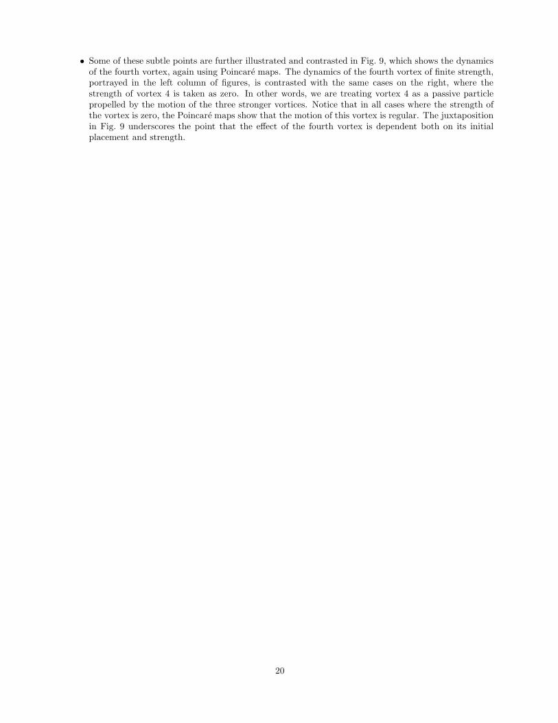
• Our main focus is on examples where the unperturbed system is of the elliptic type, i.e. cases 1, 4, 7.Initial configuration near Q3, in between two separatrices (region 3B shown in Fig. 1), and near thecenter E. We expect more sensitivity to perturbations for of any of the three types for case 4 than1 and 7, since case 4 represents a configuration closer to the separatrix shown in Fig. 1, and this isborne out by our simulations.

• The motion of the three vortices in the plane for cases 1, 4, and 7 in the unperturbed system is shownin Figure 5. Notice that even in this case, the trajectories are considerably more complicated for case4 than cases 1 and 7. Again this is due to proximity to the separatrix.

18

• For a type A perturbation with h = 10, we observe little impact on trajectories of the 3 vortices. Thisis consistent our theoretical results.

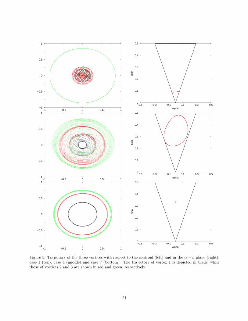
• For cases 1 and 7, we also consider lower values of h - as low as h = 2.5. For case 4 corresponding, to apoint close to the separatrix for the unperturbed system, the dynamics become much more complicatedat a more rapid pace as h decreases. The Poincare maps (x1, y1 for y2 = 0) shown in Fig. 6 suggestthat when h = 2.5 the dynamics is starting to exhibit chaotic regimes.

• Also considered in our simulations are type C perturbations. We found that it is necessary to startwith a large mean radius for the three slender coaxial vortex rings in order to observe theoreticalpredictions. With ρ = 250, the motion remains regular. This is illustrated in the Poincare maps shownin Fig. 7.

• In the final set of simulations, we considered examples of restricted four vortex dynamics The configu-ration of the three larger (principal) vortices, which we designate as vortices 1-3, is defined in terms ofequal-strength vortices, ki = 1 for i = 1, 2, 3, initially located on the vertices of an equilateral triangleof side 1. Specifically, the initial conditions are given by: z1 = (−0.5, 0), z2 = (0.5, 0), and z3 = (0, h)where h =

√3/2. For the unperturbed case, the trajectories with respect to the centroid are identical

circles centered at the origin. We consider perturbation due to the introduction of a weak vortex havingk4 = 0.1. Five different initial conditions for the fourth vortex are considered, namely z4 = (0.1, 0),z4 = (0.1, h/3), z4 = (0.1, 2h/3), z4 = (0.1, h), and z4 = (0.1, 4h/3). We refer to these as cases i - v,respectively.

• Consistent with predictions, the trajectories of vortices 1-3 are only weakly affected by the introductionof the fourth (weaker or smaller) vortex (not shown). More precisely, we find that the common circle ofmotion of the three principal vortices becomes slightly thickened (forming a thin annulus) in the plane- with the thickness of the annulus and variation of motion within it reflecting the magnitude (as wellas the particular form) of the perturbation caused by the smaller vortex. One expects the annulus tothicken when the smaller vortex starts closer to the configuration of vortices 1-3, its strength increases,or when the weaker vortex starts in a position that has a more subtle connection with the configurationof the whole set of four vortices. These subtleties will be discussed at some length in the followingpoints.

• The most dramatic effect on the dynamics for the restricted four vortex problem is naturally manifestedin the motion of the fourth (smaller or weaker) vortex. The trajectory of the fourth vortex can beeither regular or complex and even chaotic, depending on its initial location and strength. Moreover,the complexity of its trajectory is quite sensitive to changes in its initial location and strength. Thisis illustrated in the Poincare maps of (x4, y4 at y1 = 0).

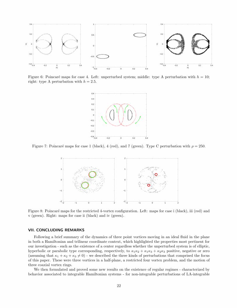
• The Poincare maps for the motion of the fourth vortex shown in Fig. 8 indicate via the characteristicsplattering that the dynamics for cases i and ii exhibit typical chaotic behavior, or at least a transitionfrom regular to chaotic motion, whereas cases iii and iv are essentially regular. This may appear tobe somewhat surprising in light of the fact that the distance from vortex 4 to the set of vortices 1-3 incases i and ii is not very different from the distances in cases iii and iv.

• A plausible explanation for the somewhat counter intuitive behavior described above is as follows: If weview vortex 4 as perturbing the motion of vortices 1-3 (see Fig. 1), we would not, as indicated above,expect this to have much effect on the dynamics of vortices 1-3. In particular, the configuration ofvortices 1-3 places it initially at the center E, so the inherent stability should preserve periodic motionfor this configuration that varies only slightly from an equilateral array. Dually, we can consider thetriple of vortices 1, 2 and 4, as being perturbed by the strong third vortex. For cases i and ii, theinitial configuration of {1, 2, 4} is rather close to a separatrix shown in Fig. 8. This experiences a strongperturbation from vortex 3, which is substantial enough to push the configuration across the separatrixand also possibly break this curve. Similarly, cases iii-v are such that the initial configuration of vorticesi, ii and iv are substantially further removed from such a separatrix, so then it is not surprising thatthe dynamics for cases i and ii is far less regular than that for cases iii and iv.

19

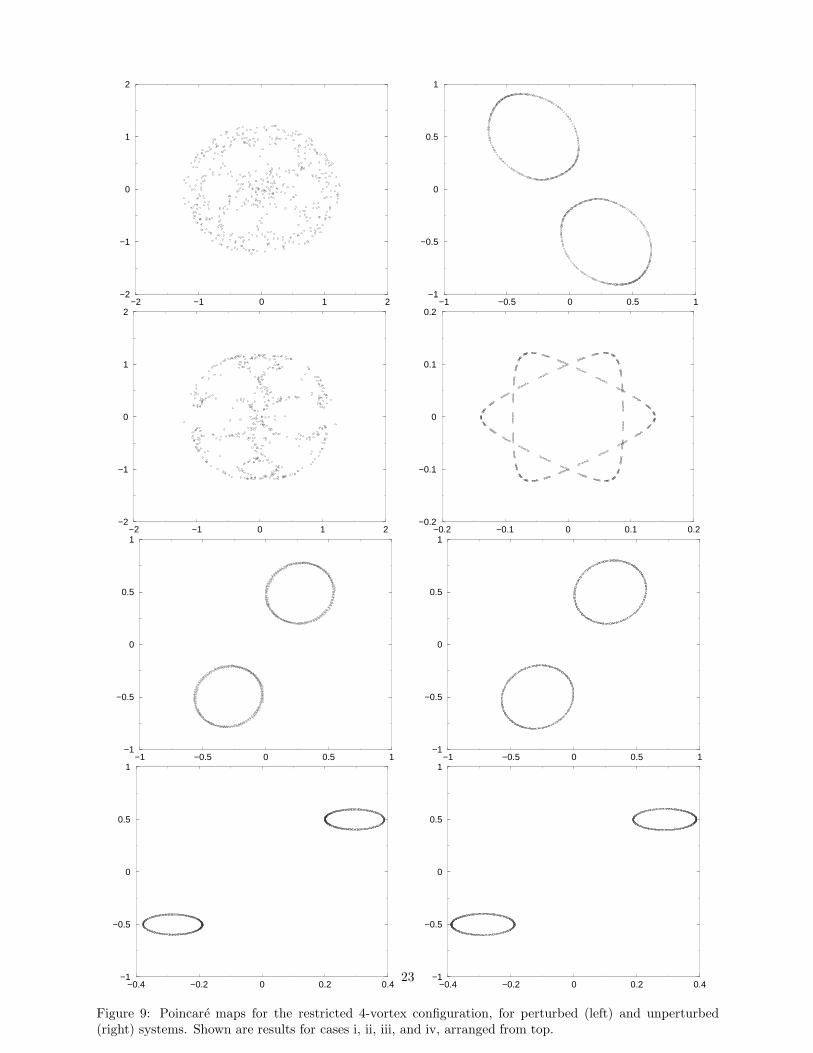
• Some of these subtle points are further illustrated and contrasted in Fig. 9, which shows the dynamicsof the fourth vortex, again using Poincare maps. The dynamics of the fourth vortex of finite strength,portrayed in the left column of figures, is contrasted with the same cases on the right, where thestrength of vortex 4 is taken as zero. In other words, we are treating vortex 4 as a passive particlepropelled by the motion of the three stronger vortices. Notice that in all cases where the strength ofthe vortex is zero, the Poincare maps show that the motion of this vortex is regular. The juxtapositionin Fig. 9 underscores the point that the effect of the fourth vortex is dependent both on its initialplacement and strength.

20

−1 −0.5 0 0.5 1−1

−0.5

0

0.5

1

−0.5 −0.3 −0.1 0.1 0.3 0.5alpha

0

0.1

0.2

0.3

0.4

0.5

beta

−1 −0.5 0 0.5 1−1

−0.5

0

0.5

1

−0.5 −0.3 −0.1 0.1 0.3 0.5alpha

0

0.1

0.2

0.3

0.4

0.5

beta

−1 −0.5 0 0.5 1−1

−0.5

0

0.5

1

−0.5 −0.3 −0.1 0.1 0.3 0.5alpha

0

0.1

0.2

0.3

0.4

0.5

beta

Figure 5: Trajectory of the three vortices with respect to the centroid (left) and in the α − β plane (right):case 1 (top), case 4 (middle) and case 7 (bottom). The trajectory of vortex 1 is depicted in black, whilethose of vortices 2 and 3 are shown in red and green, respectively.

21

−0.4 −0.2 0 0.2 0.4X1

−0.4

−0.2

0

0.2

0.4Y

1

−0.4 −0.2 0 0.2 0.4−1

−0.5

0

0.5

1

−0.4 −0.2 0 0.2 0.4X1

−0.4

−0.2

0

0.2

0.4

Y1

Figure 6: Poincare maps for case 4. Left: unperturbed system; middle: type A perturbation with h = 10;right: type A perturbation with h = 2.5.

−0.4 −0.2 0 0.2 0.4−0.4

−0.3

−0.2

−0.1

0

0.1

0.2

0.3

0.4

Figure 7: Poincare maps for case 1 (black), 4 (red), and 7 (green). Type C perturbation with ρ = 250.

−2 −1 0 1 2−2

−1

0

1

2

−2 −1 0 1 2−2

−1

0

1

2

Figure 8: Poincare maps for the restricted 4-vortex configuration. Left: maps for case i (black), iii (red) andv (green). Right: maps for case ii (black) and iv (green).

VII. CONCLUDING REMARKS

Following a brief summary of the dynamics of three point vortices moving in an ideal fluid in the planein both a Hamiltonian and trilinear coordinate context, which highlighted the properties most pertinent forour investigation - such as the existence of a center regardless whether the unperturbed system is of elliptic,hyperbolic or parabolic type corresponding, respectively, to κ1κ2 + κ1κ3 + κ2κ3 positive, negative or zero(assuming that κ1 + κ2 + κ3 6= 0) - we described the three kinds of perturbations that comprised the focusof this paper. These were three vortices in a half-plane, a restricted four vortex problem, and the motion ofthree coaxial vortex rings.

We then formulated and proved some new results on the existence of regular regimes - characterized bybehavior associated to integrable Hamiltonian systems - for non-integrable perturbations of LA-integrable

22

−2 −1 0 1 2−2

−1

0

1

2

−1 −0.5 0 0.5 1−1

−0.5

0

0.5

1

−2 −1 0 1 2−2

−1

0

1

2

−0.2 −0.1 0 0.1 0.2−0.2

−0.1

0

0.1

0.2

−1 −0.5 0 0.5 1−1

−0.5

0

0.5

1

−1 −0.5 0 0.5 1−1

−0.5

0

0.5

1

−0.4 −0.2 0 0.2 0.4−1

−0.5

0

0.5

1

−0.4 −0.2 0 0.2 0.4−1

−0.5

0

0.5

1

Figure 9: Poincare maps for the restricted 4-vortex configuration, for perturbed (left) and unperturbed(right) systems. Shown are results for cases i, ii, iii, and iv, arranged from top.

23

three vortex dynamics. The regular dynamics in point includes the existence of an ample set of quasiperiodicflows on invariant KAM tori along with periodic solutions. These results, which were proved employing rathermodern variants and generalizations of the KAM and Poincare-Birkhoff fixed point theorems, extend somerelated recent results for point and coaxial ring vortices to cases where the signs of the vortex strengthsdiffer, and are such that their sufficient conditions can be readily checked. But, they are really just existencetheorems that provide little information about the location and finer geometric details of the predictedinvariant tori and periodic orbits.

The lack of quantitative specificity in our first set of perturbation theorems was subsequently addressedfor the case of periodic orbits, with some novel results concerning the existence of periodic solutions forperturbed systems that closely approximate cycles of the unperturbed three vortex system. These results- possessing the look and feel of classical perturbation theorems - were proved using Poincare sections inconcert with the Brouwer fixed point theorem, are stated in terms of easily verifiable criteria guaranteeingthe existence of periodic orbits of the perturbed system close to those of the three vortex system.

Several numerical simulations were performed to illustrate the perturbations theorems obtained in avariety of contexts. Also included were examples to indicate how the desired regularity of the dynamicsbreaks down as the assumptions of our theorems are stretched to the limit, which is accomplished by showinghow there is a (transitional) preponderance of chaotic regimes as these limits are exceeded.

Our study of perturbations of the three vortex problem has, we hope, shed some new light on theseparticular systems as well as more general vortex phenomena. It certainly has - as is often the case in suchstudies - created more interesting questions than it has answered, several of which we intend to investigatein the near future. For example, our work here suggests that most of our results can be extended to systemscomprised of a larger number of vortex elements if they are clustered in certain ways. As an illustrationof this, suppose that one has a pair of vortices of strengths of the same sign that are initially quite closetogether. Then this pair constitutes a binary system that should, under the right conditions, remain closetogether for all time, and behave as if it were a single vortex of strength equal to the sum of the strengths ofeach of its components if any other point vortices have initial distances from this pair that are substantiallylarger than the distance between the pair. A configuration of four vortices including such a binary systemand two other vortices initially quite distant from the pair, might well be expected to behave very much likea slightly perturbed three vortex system in the plane (with the binary system acting like a single vortex),thus generating a profusion of regimes exhibiting regular (integrable type) dynamics. Interesting clusteringproblems of this kind are something that we plan to turn our attention to in our future research.

Another rather manifest question raised by our investigation - that we intend to presently turn our at-tention to - concerns extending the quantitative perturbation results obtained for periodic orbits to invarianttori. It appears that it may be possible, using some type of generalization of the Poincare-Birkhoff fixedpoint theorem, to show that in certain cases the perturbed system has an invariant torus that is close to aninvariant torus for the unperturbed system.

ACKNOWLEDGMENTS

The authors wish to dedicate this paper to Professor Theodore Yaotsu Wu of the California Institute ofTechnology, belatedly on his eightieth birthday, and to honor his life-long pioneering contributions to fluidmechanics and soliton waves, and his leadership in training younger scientists and engineers. In particular,L. T. would like to refresh his memories with Professor Wu of being classmates in the ninth grade at GuangHua Middle School and 1946 alumni of the Chioa Tung University, Shanghai.

In addition, the authors wish to express their appreciation to Charles Doering and Paul Newton, guesteditors of the special focus issue of the Journal of Mathematical Physics on mathematical fluid dynamics,for their gracious invitation to contribute this paper.

Lastly, we wish to acknowledge that preliminary versions of some of the material in this paper were re-ported on at the ICTAM Conference in Warsaw, Poland, 2004, the Third MIT Conference on ComputationalFluid and Solid Mechanics, 2005, and the GAMM Annual Meeting, Berlin, 2006, and appeared in summaryform in the proceedings of the first two conferences.

24

References

[1] H. Aref, Motion of three vortices, Phys. Fluids 22 (1979), 393-400.

[2] H. Aref, Integrable, chaotic, and turbulent motion in two-dimensional flows, Ann. Rev. Fluid Mech. 15(1983), 345-389.

[3] H. Aref and M. Stremler, Four-vortex motion with zero total circulation and impulse, Phys. Fluids 11(1999), 3704-3715

[4] V. Arnold, Small denominators and the problem of stability of motion in classical and celestial mechan-ics, Russian Math. Surveys 18 (1963), 85-91.

[5] V. Arnold, Mathematical Methods of Classical Mechanics, Springer-Verlag, New York, 1978.

[6] A. Bagrets and D. Bagrets, Non-integrability of two problems in vortex dynamics, Chaos 7 (1997),368-375.

[7] G. Birkhoff, An extension of Poincare’s last geometric theorem, Acta Math. 47 (1925), 210-231.

[8] D. Blackmore and O. Knio, KAM theory analysis of the dynamics of three coaxial vortex rings, PhysicaD 140 (2000), 321-348.

[9] D. Blackmore and O. Knio, Transition from quasiperiodicity to chaos for three coaxial vortex rings,ZAMM 80 S (2000), 173-176.

[10] D. Blackmore and C. Wang, Morse index for autonomous linear Hamiltonian systems, Int. J. Diff. Eqs.and Appl. 7 (2003), 295-309.

[11] D. Blackmore, J. Champanerkar and C. Wang, A generalized Poincare-Birkhoff theorem with applica-tions to coaxial vortex ring motion, Discrete and Contin. Dyn. Syst.-B 5 (2005), 15-33.

[12] D. Blackmore, L. Ting and O. Knio, Motion of three point vortices, Proc. 3 rd MIT Conf. on Comp.Fluid and Solid Mech., June, 2005.

[13] D. Blackmore and J. Champanerkar, Periodic and quasiperiodic motion of point vortices, Vortex Dom-inated Flows, D. Blackmore, E. Krause and C. Tung (eds.), World Scientific, Singapore, 2005, pp.21-42.

[14] V. Bogomolov, Two-dimensional fluid dynamics on a sphere, Izv. Atmos. Oc. Phys. 15 (1979), 18-22.

[15] A. Borisov and V. Lebedev, Dynamics of three vortices on a plane and a sphere - II, Regul. ChaoticDyn. 3 (1998), 99-114.

[16] A. Borisov, I. Mamaev and A. Kilin, Absolute and relative choreographies in the problem of pointvortices moving on a plane, Reg. & Chaot. Dyn. 9 (2004), 101-111. 99-114.

[17] A. Borisov, I. Mamaev and A. Kilin, New periodic solutions for three or four identical vortices on aplane and sphere. arXiv.nlin.SI/0507058 v1 26 Jul 2005.

[18] A. Callegari and L. Ting, Motion of a curved vortex filament with decaying vortical core and axialvelocity, SIAM J. Appl. Math. 35 (1978), 148-175.

[19] A. Carter, An improvement of the Poincare-Birkhoff fixed point theorem, Trans. Amer. Math. Soc. 269(1982), 285-299.

[20] A. Celletti and C. Falcolini, A remark on the KAM theorem applied to a four vortex system, J. Stat.Phys. 52 (1988), 471-477.

[21] C. Conley and E. Zehnder, The Birkhoff-Lewis fixed point theorem and a conjecture of V. I. Arnold,Invent. Math.73 (1983), 207-253.

25

[22] W.Y. Ding, A generalization of the Poincare-Birkhoff theorem, Proc. Amer. Math. Soc. 88 (1983),341-346.

[23] B. Eckhardt, Integrable four vortex motion, Phys. Fluids 31 (1988), 2796-2801.

[24] A. Floer, Symplectic fixed points and holomorphic spheres, Comm. Math. Phys. 120 (1989), 575-611.

[25] J. Franks, Generalizations of the Poincare-Birkhoff theorem, Annals of Math. 128 (1988), 139-151.

[26] C. Gole, Symplectic Twist Maps, World Scientific, Singapore, 2001.

[27] D. Goryachev, On Certain Cases of Motion of Rectilinear Parallel Vortices, Moscow University PrintingHouse, Moscow, 1898. (in Russian)

[28] W. Grobli, Speciale Probleme uber die Bewegung Geradliniger Paralleler Wirbelfaden, Zurcher andFurrer, Zurich, 1877.

[29] H. Helmholtz, Uber integrale hydrodynamischen gleichungen weiche den wirbelbewegungen entsprechen,J. Reine Angew. Math. 55 (1858), 25-225.

[30] F. Josellis, Lyusternik-Schnirelman theory for flows and periodic orbits for Hamiltonian systems on Tn

× Rn, Proc. London Math. Soc. 68 (1994), 641- 672.

[31] A. Katok and B. Hasselblatt, Introduction to the Modern Theory of Dynamical Systems, CambridgeUniversity Press, Cambridge, 1995.

[32] K. Khanin, Quasi-periodic motion of vortex systems, Physica D 4 (1982), 261-269.

[33] G. Kirchhoff, Vorlesungen uber Mathematische Physik, Vol. 1, Teubner, Leipzig, 1876.

[34] R. Kidambi and P. Newton, Motion of three point vortices on a sphere, Physica D 116 (1998), 143-175.

[35] R. Kidambi and P. Newton, Point vortex motion on a sphere with solid boundaries, Phys. Fluids 12(2000), 581-588.

[36] O. Knio, L. Collerec and Juve, Numerical study of sound emission by 2D regular and chaotic vortexconfigurations, J. Comput. Phys. 116 (1995), 226-246.

[37] L. Kuznetsov and G. Zaslavsky, Regular and chaotic advection in the flow field of a three-vortex system,Phys. Rev. E 58 (1998), 7330-7349.

[38] H. Lamb, Hydrodynamics, Dover, New York, 1932.

[39] C.C. Lim, Existence of KAM tori in the phase-space of lattice vortex systems, ZAMP 41 (1990), 227-244.

[40] C.C. Lim, Relative equilibria of symmetric N-body problems on a sphere: inverse and direct results,Comm. Pure Appl. Math. 51 (1998), 341-371.

[41] C.C. Lin, On the Motion of Vortices in Two Dimensions, Toronto University Press, Toronto, 1943.

[42] J. Moser, Stable and Random Motions in Dynamical Systems, Princeton Univ. Press, Princeton, 1973.

[43] J. Moser, Proof of a generalized form of the fixed point theorem due to G. D. Birkhoff, Geometry andTopology, Lecture Notes in Math., 597, Springer-Verlag, New York, 1977.

[44] P. Newton, The N-Vortex Problem: Analytical Techniques, Springer-Verlag, New York, 2001.

[45] E. Novikov, Dynamics and statistics of a system of vortices, Sov. Phys. JETP 41 (1975), 937-943.

[46] H. Poincare, Sur un theoreme de geometrie, Rend. del. Circ. Math. du Palermo 33 (1912), 375-407.

[47] H. Poincare, Theorie des Tourbillons, G. Carre (ed.), Deslis Freres, Paris, 1983.

26

[48] C. Robinson, Generic properties of conservative systems I; II, Amer. J. Math. 92 (1970), 562-603;897-906.

[49] T. Sakajo, Integrable four-vortex motion on sphere with zero moment of vorticity. (preprint)

[50] M. Sokolovskiy and J. Verron, Four-vortex motion in the two layer approximation: integrable case,Regul. Chaotic Dyn. 5 (2000), 413-436.

[51] E. Spanier, Algebraic Topology, McGraw-Hill, New York, 1966.

[52] J. Synge, On the motion of three vortices, Can. J. Math. 1 (1949), 257-270.

[53] J. Tavantzis and L. Ting, The dynamics of three vortices revisited, Phys. Fluids 31 (1988),1392-1409.

[54] L. Ting and R. Klein, Viscous Vortical Flows, Lecture Notes in Physics, Vol. 374, Springer-Verlag,Berlin, 1991.

[55] L. Ting and D. Blackmore, Bifurcation of motions of three vortices and applications, Proc. 2004 ICTAMConf., Warsaw, 2004.

[56] L. Ting, D. Blackmore and O. Knio, Perturbed three point vortex problems - the parabolic case. (inpreparation)

[57] T. Tokieda, Tourbillons dansants, C. R. Acad. Sci. Paris Serie I 333 (2001), 943-946.

[58] S. Ziglin, The non-integrability of the problem of motion of four vortices of finite strengths, Physica D4 (1982), 268-269.

27

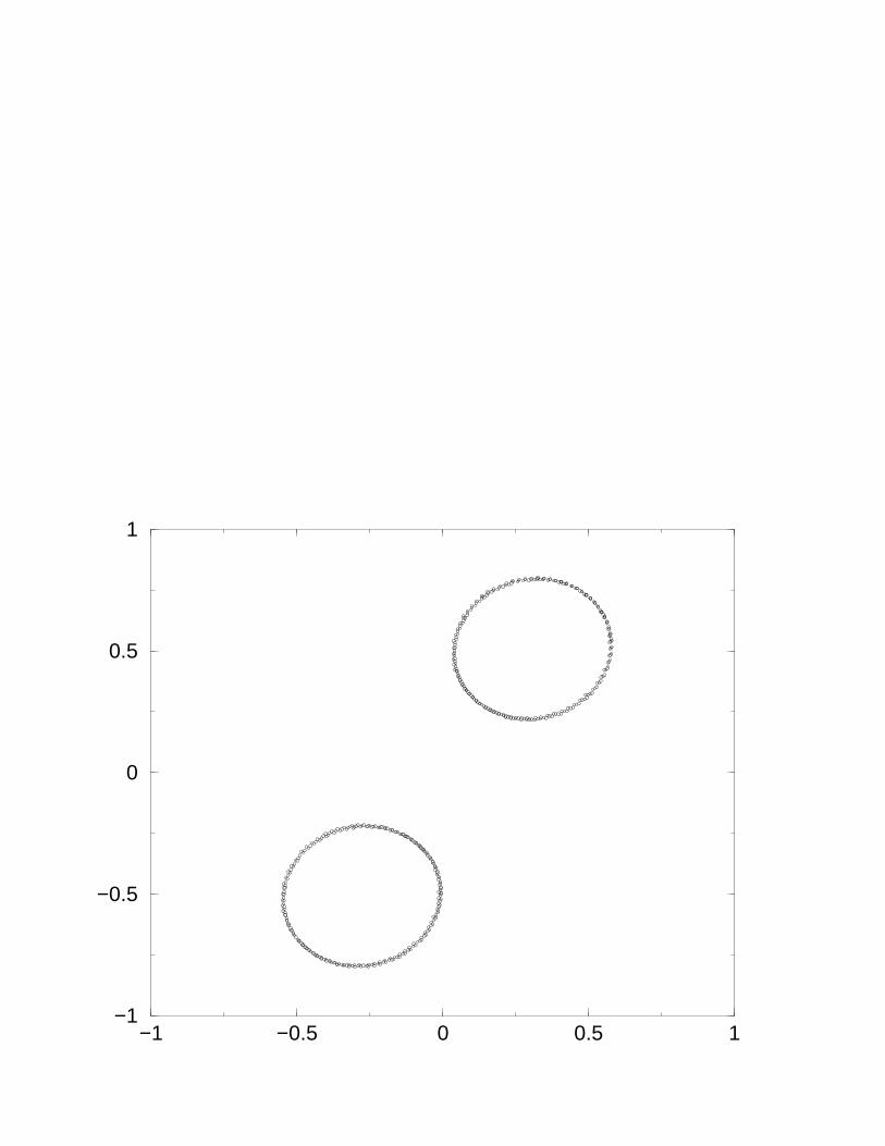
−1 −0.5 0 0.5 1−1

−0.5

0

0.5

1

−1 −0.5 0 0.5 1−1

−0.5

0

0.5

1