HAL Id: tel-03065015 https://tel.archives-ouvertes.fr/tel-03065015v2 Submitted on 17 Dec 2020 HAL is a multi-disciplinary open access archive for the deposit and dissemination of sci- entific research documents, whether they are pub- lished or not. The documents may come from teaching and research institutions in France or abroad, or from public or private research centers. L’archive ouverte pluridisciplinaire HAL, est destinée au dépôt et à la diffusion de documents scientifiques de niveau recherche, publiés ou non, émanant des établissements d’enseignement et de recherche français ou étrangers, des laboratoires publics ou privés. Strongly-correlated one-dimensional bosons in continuous and quasiperiodic potentials Hepeng Yao To cite this version: Hepeng Yao. Strongly-correlated one-dimensional bosons in continuous and quasiperiodic potentials. Quantum Gases [cond-mat.quant-gas]. Institut Polytechnique de Paris, 2020. English. NNT: 2020IP- PAX057. tel-03065015v2

Welcome message from author
This document is posted to help you gain knowledge. Please leave a comment to let me know what you think about it! Share it to your friends and learn new things together.
Transcript

HAL Id: tel-03065015https://tel.archives-ouvertes.fr/tel-03065015v2
Submitted on 17 Dec 2020
HAL is a multi-disciplinary open accessarchive for the deposit and dissemination of sci-entific research documents, whether they are pub-lished or not. The documents may come fromteaching and research institutions in France orabroad, or from public or private research centers.
L’archive ouverte pluridisciplinaire HAL, estdestinée au dépôt et à la diffusion de documentsscientifiques de niveau recherche, publiés ou non,émanant des établissements d’enseignement et derecherche français ou étrangers, des laboratoirespublics ou privés.
Strongly-correlated one-dimensional bosons incontinuous and quasiperiodic potentials
Hepeng Yao
To cite this version:Hepeng Yao. Strongly-correlated one-dimensional bosons in continuous and quasiperiodic potentials.Quantum Gases [cond-mat.quant-gas]. Institut Polytechnique de Paris, 2020. English. NNT : 2020IP-PAX057. tel-03065015v2
626
NN
T:2
020I
PPA
X05
7
Strongly-correlated one-dimensionalbosons in continuous and quasiperiodic
potentialsThese de doctorat de l’Institut Polytechnique de Paris
preparee a l’Ecole polytechnique
Ecole doctorale n626 de l’Institut Polytechnique de Paris (IP Paris)Specialite de doctorat : Physique
These presentee et soutenue a Palaiseau, le 20/10/2020, par
HEPENG YAO
Composition du Jury :
Thierry GiamarchiProfesseur, University of Geneva (Department of Quantum MatterPhysics) President
Guillaume RouxMaıtre de conferences, Universite Paris-Saclay (Le Laboratoire dePhysique Theorique et Modeles Statistiques) Rapporteur
Ulrich SchneiderProfesseur, University of Cambridge (Cavendish Laboratory) Rapporteur
Anna MinguzziDirecteur de recherche, Universite Grenoble Alpes (Laboratoire dePhysique et Modelisation des Milieux Condenses) Examinateur
Hanns-Christoph NagerlProfesseur, University of Innsbruck (Institute for ExperimentalPhysics) Examinateur
Laurent Sanchez-PalenciaDirecteur de recherche, Ecole polytechnique (Centre de PhysiqueTheorique)
Directeur de these


Acknowledgements
The work reported in this manuscript was carried out in the Centre de PhysiqueThéorique (CPHT) of École Polytechnique, located in Palaiseau, France. This thesisis funded by DIM-SIRTEQ via the Centre National de la Recherche Scientifique(CNRS). The first two years of the thesis was done under the doctor school École doc-torale ondes et matière (EDOM) and during the final year, I was transferred to thedoctor school École doctorale de l’Institut Polytechnique de Paris (ED IP Paris).I want to thank all of the above institutions for providing the framework of the thesis, aswell as their staff for the valuable support on the administrative aspect.
First of all, I would like to express my deep gratitude to my supervisor LaurentSanchez-Palencia. It is well-known how important the period of PhD is for those whowants to become a permanent researcher in the future, and I’m extremely lucky to haveLaurent as my supervisor in this period. When guiding my thesis, he was always availableto answer my questions, with great patience, kind, as well as enlightening ideas and expla-nations. I really learn a lot from him, not only for details about the certain projects wewere studying, but also on how to perform a good research. His personality is a very goodexample for me which will shape me to be a good researcher in the future. Also, he wasalways trying his best to provide the best environment of research for me, on the aspectsof computing resources, administrative issues, attending conferences and etc, which allowsme to focus on research without additional worries.
Also, I would like to thank Jean-René Chazottes, the director of Centre de PhysiqueThéorique. In spite of his busy schedule, he is always very kind, helpful and supportive forall the things which guarantees the PhDs to work under the best condition. Also, I wouldlike to thank Silke Biermann, who is the coordinator of the condensed matter group, aswell as the head of physics department now. On the one side, she was always providingus necessary informations and supports as a role of coordinator. On the other side, as a"colleague next door", it’s a good memory to have those interesting discussions with herduring those "long lunch", coffee break, barbecue and etc.
Then, I would like to thank the members of my PhD committee whom I have hugerespect for. I would like to thank Guillaume Roux and Ulrich Schneider for kindlyaccepting to be the referees, and I want to thank them for their interest of reading thethesis. I would also like to thank Thierry Giamarchi, Anna Minguzzi, and Hanns-Christophe Nägerl for being the examinators.
During my PhD studies, numbers of collaborations have been carried out inside oroutside the groups. I would like to thank Anna Minguzzi and Patrizia Vignolo forour collaborations on the Tan’s contact project, especially for the beautiful analyticalcalculation of the contact formula they have provided. I would like to thank ThierryGiamarchi for our collaborations on the Bose glass project, where we have several wavesof stimulating discussions in Leiden, Palaiseau and Geneva. I would like to thank RonanGautier, Hakim Koudhli, Léa Bresque, Marco Biroli and Alessandro Pacco, forour collaborations on different projects of quasiperiodic systems. It’s interesting to workwith master and bachelor students serving as a role of "quasi-supervisor" and I reallybenefit a lot from this experience for my future career. Special thanks should be dedicated
3
to Ronan, with whom we develop the QMC code to 2D and make the code much moreefficient. Thanks to the talent of Ronan on numerics, we achieved huge progress on the codein 6 months which seems impossible for such a short period. The last and special thanks inthis part should be delivered toDavid Clément, who has always been a strong support forus from the experimental aspect. I want to thank him not only for our collaboration on theTan contact paper, but also for our further collaborations on the contact’s measurementand suggestions on our quasiperiodic project as an experimentalist. I would also like tothank the members of him team, Antoine Ténart, Gaétan Herce, Marco Mancini,Hugo Cayla, Cécile Carcy.
The next wave of thanks should be given to my great colleagues in CPHT. I would liketo firstly thank the members of our group, Steven Thompson, Julien Despres, LouisVilla, Jan Schneider. Ronan Gautier, Hakim Koudhli, Léa Bresque, MarcoBiroli and Alessandro Pacco. Special thanks should be dedicated to Louis, not onlyfor his strong support on analytical aspect of many problems and the French abstract ofthe thesis, but also for the tennis session we had each week. This provided us a goodrelax between research on physics (and probably also prepared us well for Roland Garros).Moreover, I would also like to thank Jan for the nice coffee you’ve made for us. And Iwould like to thank Zhaoxuan and Kim for the typos you found in the first version ofthe manuscript. Beyond our group, I would also like to thank some other members of thecondensed matter group, Steffen Backes, Alaska Subedi, Leonid Pourovskii, MichelFerrero, Benjamin Lenz, Anna Galler, Sumanta Bhandary, Jakob Steinbauer,Benjamin Labrueil, James Bouse,Marcello Turtulici. With all the names mentionedin this paragraph, we had so many nice discussions, lunches, coffee breaks and etc, whichmakes my stay in Palaiseau fruitful and enjoyable.
Furthermore, the administrative department and IT department are extremely power-ful and helpful. I would like to thank the administrative department of CPHT, FlorenceAuger, Malika Lang, Fadila Debbou. Your high efficiency of work makes all thecomplicated administrative work easy for me. Also, I would also like to thank the ITdepartment, Jean-Luc Bellon, Danh Pham Kim, Yannick Fitamant as well as Au-rélien Canou as advisory support. With all your explanations and discussions of months,we finally install the QMC code and run it successfully on the cluster which seems like animpossible task at the very beginning. You also provided invaluable support for all kindsof numerical issues during my PhD.
During the three years of PhD, my family is always a strong support from my back. Myfather Bingliang Yao and mother Aijun Liu have always been supportive and helpfulfor me doing the PhD abroad. No matter whenever I need help from them, they are alwaystrying their best to help me from seven thousands miles away. Also, I’m grateful to myfather for his stimulating education, which makes me a physicists with strong ability onnumerics, and to my mother for her strong ability on cooking which makes my vacationback in China enjoyable. Moreover, I want to thank my grandparents, my aunts, unclesand cousins, who always welcome me back to Beijing during summer or winter vacations.Finally, I want to thank my girlfriend Wenwen Li, who stays with me in Massy duringthe period of thesis writing. The process of writing thesis can be sometimes torturedmentally, and the confinement of COVID-19 pushes it to a harder situation. Thanks toher accompany, patience, kind and humor, I can keep calm and faithful during the writingperiod. The positive attitude you shared with me in this special period is an invaluablesupport for me which is decisive for the completion of this work.
4

Contents
Introduction 7
Résumé 10
1 Bosons in One Dimension 131.1 The general interest of one dimensional bosons . . . . . . . . . . . . . . . . 141.2 One-dimensional bosons in the continuum . . . . . . . . . . . . . . . . . . . 15
1.2.1 Lieb-Liniger bosons and delta-range interaction . . . . . . . . . . . . 151.2.2 One-dimensional bosons at zero temperature and Bethe ansatz . . . 161.2.3 One-dimensional bosons at finite temperature and Yang-Yang ther-
modynamics . . . . . . . . . . . . . . . . . . . . . . . . . . . . . . . . 201.2.4 The field description: Luttinger liquid theory . . . . . . . . . . . . . 22
1.3 One-dimensional bosons in a lattice . . . . . . . . . . . . . . . . . . . . . . . 231.3.1 One-dimensional Bose-Hubbard model . . . . . . . . . . . . . . . . . 241.3.2 One-dimensional bosons in shallow periodic lattice . . . . . . . . . . 271.3.3 One-dimensional bosons in purely-disordered potentials . . . . . . . 31
2 Continuous-space quantum Monte Carlo for bosons 332.1 Path-integral Monte Carlo for interacting bosons . . . . . . . . . . . . . . . 34
2.1.1 Feynman path integral for a single particle . . . . . . . . . . . . . . . 342.1.2 Feynman path integral for many-body bosonic systems . . . . . . . . 362.1.3 The imaginary time propagator . . . . . . . . . . . . . . . . . . . . . 382.1.4 Sampling the configurations using the Monte Carlo approach . . . . 402.1.5 Standard moves for path-integral Monte Carlo . . . . . . . . . . . . . 43
2.2 Worm algorithm . . . . . . . . . . . . . . . . . . . . . . . . . . . . . . . . . 452.2.1 The winding number . . . . . . . . . . . . . . . . . . . . . . . . . . . 462.2.2 The extended partition function: Z-sector and G-sector . . . . . . . 462.2.3 Monte Carlo moves in the worm algorithm . . . . . . . . . . . . . . . 48
2.3 Computation of observables . . . . . . . . . . . . . . . . . . . . . . . . . . . 512.3.1 Particle density and compressibility . . . . . . . . . . . . . . . . . . . 512.3.2 Superfluid density . . . . . . . . . . . . . . . . . . . . . . . . . . . . 522.3.3 Green’s function . . . . . . . . . . . . . . . . . . . . . . . . . . . . . 532.3.4 Correlation function and momentum distribution . . . . . . . . . . . 54
3 Tan’s contact for trapped Lieb-Liniger bosons at finite temperature 563.1 Two-parameter scaling function . . . . . . . . . . . . . . . . . . . . . . . . . 58
3.1.1 The two-parameter scaling . . . . . . . . . . . . . . . . . . . . . . . . 583.1.2 Computing the scaling function using the Yang-Yang theory . . . . . 613.1.3 Validation of the scaling function using quantum Monte Carlo . . . . 62
3.2 The behavior of the contact and regimes of degeneracy . . . . . . . . . . . . 653.2.1 The behavior of the contact in the homogeneous case . . . . . . . . . 663.2.2 The scaling function in different regimes . . . . . . . . . . . . . . . . 66
5

3.2.3 The onset of maximum . . . . . . . . . . . . . . . . . . . . . . . . . . 713.3 Experimental observability . . . . . . . . . . . . . . . . . . . . . . . . . . . . 74
3.3.1 Accuracy of detection . . . . . . . . . . . . . . . . . . . . . . . . . . 743.3.2 Validity condition of the quasi-1D regime . . . . . . . . . . . . . . . 743.3.3 Tube distributions . . . . . . . . . . . . . . . . . . . . . . . . . . . . 75
4 Critical behavior in shallow 1D quasiperiodic potentials: localization andfractality 784.1 Localization, disorder and quasiperiodicity . . . . . . . . . . . . . . . . . . . 80
4.1.1 Basic concepts for localization . . . . . . . . . . . . . . . . . . . . . . 804.1.2 Localization in different kinds of system . . . . . . . . . . . . . . . . 81
4.2 Critical localization behavior in 1D shallow quasiperiodic lattices . . . . . . 834.2.1 The localization properties of balanced bichromatic lattices . . . . . 834.2.2 Other quasi-periodic lattices and universality . . . . . . . . . . . . . 87
4.3 The fractality of the energy spectrum . . . . . . . . . . . . . . . . . . . . . . 924.3.1 Fractals and fractal dimension . . . . . . . . . . . . . . . . . . . . . . 924.3.2 Fractality of the energy spectrum for 1D quasiperiodic systems . . . 964.3.3 Properties of the spectrum fractal dimension . . . . . . . . . . . . . 100
5 Lieb-Liniger bosons in a shallow quasiperiodic potential 1025.1 The Bose glass phase . . . . . . . . . . . . . . . . . . . . . . . . . . . . . . . 103
5.1.1 Bose glass phase in random potentials . . . . . . . . . . . . . . . . . 1045.1.2 Bose glass phase in quasiperiodic Bose-Hubbard model . . . . . . . . 106
5.2 The phase diagram for the shallow quasiperiodic systems . . . . . . . . . . . 1125.2.1 Quantum Monte Carlo calculations for the determination of the phase1135.2.2 Analysis of the phase diagram . . . . . . . . . . . . . . . . . . . . . . 116
5.3 Finite temperature effects . . . . . . . . . . . . . . . . . . . . . . . . . . . . 1175.3.1 The melting of the quantum phases . . . . . . . . . . . . . . . . . . . 1175.3.2 Fractal Mott lobes . . . . . . . . . . . . . . . . . . . . . . . . . . . . 121
6 Conclusion and perspectives 125
Appendix 128
List of publications 130
Bibliography 131
Introduction
"Upward, not northward", this is the famous sentence in the book "Flatland" by EdwinA. Abbott, where a two-dimensional (2D) square is given a glimpse of three-dimensional(3D) truth. This is the mantra he repeats, although he ends up dying without anyone inhis world believing him. This book marks one of the first time that people perceives thepower of dimensionality. In the nature, dimensionality plays a strong role. Although oneof the main interest is to detect the existence of higher dimension in the context of highenergy physics, understanding dimension lower than 3 is also valuable and interesting inmany other fields.
In quantum physics, low dimensions are particularly rich. For instance, two-dimensionalquantum systems appear to be extremely suitable for the study of topological effects,vortex physics and rotational ring structure [1]. Also, as pointed out by Refs. [1–3], theone-dimensional bosons have its special peculiarities such as the collective property ofexcitations, the power law decay of the correlation functions, as well as the fermionizationof strongly-interacting bosons. More detailed discussion for the speciality of 1D bosonswill be presented in the first chapter of this thesis.
From the experimental point of view, the achievement of Bose-Einstein condensatesand ultracold Fermi seas since the second half of the 1990’s have opened a new avenue tostudy three-dimensional quantum systems, but also in the lower dimensions [4–8]. Withthe development of quantum optics, people can change the dimensionality of the quantumsystems and constrain one or two spatial dimensions with an attractive laser light, opticallattices and atom chips [9–12]. Various research has been carried out in low dimensionalquantum systems [1, 9–39].
One-dimensional bosons is one of those low dimensional quantum systems which haveattracted much attentions. In the continuum, they exhibit a special property called"fermionization" in the strongly-interacting limit, which is also known as the Tonks-Girardeau gases [40]. In 2004, these special gases have firstly been achieved experimentally,see Refs [9,10]. Also, in the presence of periodic lattices or disorder, they show propertiesof quantum phase transition different from 3D, see examples in Refs. [13–16,41]. It opensa new area of research where exists fruitful physics to be explored.
Understanding the quantum phase transitions as well as regime crossovers is one of themain topics in quantum statistical physics. In the field of ultracold atoms, the superfluid-Mott insulator transition in lattice systems is the most well-studied one, since this isa good quantum simulator for the conductance-insulator transition in condensed matterphysics [13,15,42,43]. However, it is also interesting to investigate other types of systems,for instance: (i) For continuous systems, the quantum gas can have different regimes ofdegeneracy depending on temperature, interactions and etc. (ii) In the presence of disorderor quasi-disorder, they can exhibit localization transitions.
In this manuscript, we theoretically study the properties of one-dimensional bosons invarious types of systems, focusing on the phase transitions or crossovers between differentquantum degeneracy regimes. Thanks to advanced quantum Monte Carlo simulationscomplemented by exact diagonalization and Yang-Yang thermodynamics, we can study
7

0. Introduction
the properties of 1D bosons in various situations where the results are still lacking. Themain results of the thesis constitute three parts. Firstly, focusing on the 1D harmonicallytrapped continuous bosons, we give a full characterization of the quantity called "Tan’scontact" for arbitrary interactions and temperature. This is a experimentally measurablequantity which provides fruitful information about the system, such as the interactionenergy and the variation of the grand potential. Our results turn out to show that thisquantity gives a good characterization for different regimes. Especially, in the strongly-interacting regime, we find the Tan contact behaves non-monotonously versus temperatureand exhibits a maximum which is the signature of the crossover to the fermionization atfinite temperature, where other quantities always behave motononously. Secondly, we turnto the study of the localization properties of the 1D ideal gas in shallow quasiperiodicpotentials. In the previous works, the localization problems in the tight-binding Aubry-André (AA) model have been extensively studied. The shallow lattice case is much lessexplored. However, it is interesting because it’s different from the AA model and maycure the severe temperature problems in the ultracold atom systems. With the help ofexact diagonalization, we find the universal critical behaviors for the critical potential,mobility edge as well as the critical exponent. Also, we study in detail the fractality ofthe energy spectrum and propose a method to calculate the fractal dimension. We findthe fractal dimension is always smaller than one, which proves that the energy spectrumis nowhere dense and the mobility edge always stays in the band gap. Finally, we furtherstudy the quantum phase transition for the 1D interacting bosons in shallow quasiperiodiclattices. Similarly as the non-interacting case, the phase diagram has been widely studiedin the deep lattice case in previous work where the temperature effect is not negligible.With the help of large scale QMC calculations, we determine the phase diagrams forshallow quasiperiodic lattices, where an incompressible insulator Bose glass phase appearsin between the superfluid and Mott insulator. Then, we also investigate the thermal effectsand find the stability of Bose glass against the finite temperature, which is strongly relevantfor experimental observability. Moreover, by studying the melting of the Mott lobes, wefind its structure is fractal-like and this property can be linked with the fractality of thesingle-particle spectrum.
The manuscript is organized as follows.
First of all, in Chapter 1 and 2, we give the introductions to the physics of 1D bosonsand to the numerical approaches we shall extensively use in the remainder of the thesis,namely quantum Monte Carlo.
Chapter 1: We start with an introduction of bosons in one dimension. We firstexplain the general interest of 1D bosons. Then, we introduce the two main approachesfor describing the 1D continuous bosons, i.e. the Lieb-Liniger model and the Luttingerliquid theory. Finally, we turn to the case of 1D bosons in a lattice. We focus on the caseof tight-binding limit Bose-Hubbard model as well as the case of the shallow lattice, andexplain the known results explored in the 2010’s.
Chapter 2: We give an introductory presentation for the quantum Monte Carlo(QMC) approach we used in most of the following parts of the thesis. It is the pathintegral Monte Carlo approach in continuous space with worm algorithm implementations.We first present the basic path integral Monte Carlo with basic moves. Then, we presentthe worm algorithm which is an implementation that improves the computation efficiency.And we explain in the end the way of computing relevant observables.
Then, in the Chapters 3 to 5, we present the main results of this manuscript.
Chapter 3: We study a quantity called "Tan’s contact" for 1D bosons which has be-
8

0. Introduction
come pivotal in the description of quantum gases. We provide a full characterization ofthe Tan contact in harmonic traps with arbitrary temperatures and interactions. Com-bining the thermal Bethe ansatz, local-density approximation and quantum Monte Carlocalculations, we have shown the contact follows a universal two-parameters scaling and wedetermine the scaling function. We identify the behavior of the contact in various regimewhich characterizes the degeneracy for 1D bosons in continuum. Especially, we find thetemperature dependence of the contact displays a maximum and it provides an unequiv-ocal signature of the crossover to the fermionized regime, which is accessible in currentexperiments.
Chapter 4: We then study the critical behavior for 1D ideal gases in shallow quasiperi-odic potentials. The quasiperiodic system provides an appealing intermediate betweenlong-range ordered and genuine disordered systems with unusual critical properties. Here,we determine the critical localization properties of the single-particle problem in 1D shal-low quasiperiodic potentials. On the one hand, we determine the properties of criticalpotential amplitude, mobility edge and inverse participation ratio (IPR) critical exponentswhich are universal. On the other hand, we calculate the fractal dimension of the energyspectrum and find it is non-universal but always smaller than unity, hence showing thatthe spectrum is nowhere dense and the mobility edge is always in a gap.
Chapter 5: We further study the case of 1D interacting bosons in shallow quasiperiodiclattices. The interplay of interaction and disorder in correlated Bose fluid leads to theemergence of a compressible insulator phase known as the Bose glass. While it has beenwidely studied in the tight-binding model, its observation remains elusive owing to thetemperature effect. Here, with the large scale QMC calculations, we compute the fullphase diagrams for the Lieb-Liniger bosons in shallow quasiperiodic lattices where theissue may be overcome. A Bose glass phase, surrounded by superfluid and Mott insulator,is found above a critical potential and for finite interactions. At finite temperature, we findthe Bose glass phase is robust against thermal fluctuations up to temperatures accessiblein current experiments of quantum gases. Also, we show that the melting of the Mott lobesis a characteristic of the fractal structure.
Chapter 6: We summarize the main results obtained in this work and give an outlookon it, from both theoretical and experimental points of view.
9
Résumé
"Vers le haut, pas vers le nord", telle est la célèbre phrase du livre "Flatland" d’Edwin A.Abbott, où un carré en deux dimensions (2D) laisse entrevoir une vérité en trois dimensions(3D). C’est le mantra qu’il répète, bien qu’il finisse par mourir sans que personne dans sonmonde ne le croit. Ce livre marque l’une des premières fois où les gens perçoivent le pouvoirde la dimensionnalité. Dans la nature, la dimensionnalité joue un rôle important. Bien quel’un des principaux intérêts soit de détecter l’existence d’une dimension supérieure dans lecontexte de la physique des hautes énergies, la compréhension de la dimension inférieure à3 est également précieuse et intéressante dans de nombreux autres domaines.
En physique quantique, les basses dimensions sont particulièrement riches. Par exem-ple, les systèmes quantiques bidimensionnels sont extrêmement adaptés à l’étude des effetstopologiques, de la physique des tourbillons et de la structure des anneaux de rotation [1].En outre, comme le soulignent les Réfs. [1–3], les bosons unidimensionnels ont leurs partic-ularités telles que les propriétés collectives des excitations, la décroissance des fonctions decorrélation en loi de puissance, ainsi que la fermionisation des bosons à forte interaction.Une discussion plus détaillée de la spécificité des bosons 1D sera présentée dans le premierchapitre de cette thèse.
D’un point de vue expérimental, la réalisation de condensats de Bose-Einstein et demers de Fermi ultra-froides depuis la seconde moitié des années 1990 a ouvert une nou-velle voie pour l’étude des systèmes quantiques tridimensionnels, mais aussi en dimensionsinférieures [4–8]. Avec le développement de l’optique quantique, on peut changer la di-mension des systèmes quantiques et contraindre une ou deux dimensions spatiales avecune lumière laser attractive, des réseaux optiques et des puces atomiques [9–12]. Diversesrecherches ont été menées sur les systèmes quantiques de faible dimension [1, 9–39].
Les bosons unidimensionnels sont l’un de ces systèmes quantiques en basse dimensionqui ont attiré beaucoup d’attention. Dans le continu, ils présentent une propriété spécialeappelée "fermionisation" dans la limite de forte interaction, qui est également connue sousle nom de gaz de Tonks-Girardeau [40]. En 2004, ces gaz particuliers ont été obtenus pourla première fois expérimentalement, voir les Réfs. [9,10]. En outre, en présence de réseauxpériodiques ou de désordre, ils présentent des propriétés de transition de phase quantiquedifférentes de celles de la 3D, voir les exemples les Réfs. [13–16,41]. Cela ouvre un nouveaudomaine de recherche où il existe une physique fructueuse à explorer.
La compréhension des transitions de phase quantique et crossovers est l’un des princi-paux sujets de la physique statistique quantique. Dans le domaine des atomes ultra-froids,la transition superfluide-isolant de Mott dans les systèmes de réseaux est la plus étudiée,car c’est un bon simulateur quantique pour la transition conducteur-isolant en physiquede la matière condensée [13, 15, 42, 43]. Cependant, il est également intéressant d’étudierd’autres types de systèmes, par exemple : (i) Pour les systèmes continus, le gaz quantiquepeut présenter différents régimes de dégénérescence en fonction de la température, des in-teractions, etc. (ii) En présence de désordre ou de quasi-désordre, ils peuvent présenterdes transitions de localisation.
10

0. Résumé
Dans ce manuscrit, nous étudions théoriquement les propriétés des bosons unidimen-sionnels dans différents types de systèmes, en nous concentrant sur les transitions de phaseou les crossovers entre différents régimes de dégénérescence quantique. Grâce à des simula-tions de Monte Carlo quantique avancées, complétées par des approches de diagonalisationexacte et la thermodynamique Yang-Yang, nous pouvons étudier les propriétés des bosons1D dans diverses situations où les résultats font encore défaut. Les principaux résultats dela thèse consituent trois parties. Premièrement, en se concentrant sur les bosons continus1D piégés de manière harmonique, nous donnons une caractérisation complète de la quan-tité appelée "contact de Tan" pour des interactions et des températures arbitraires. Il s’agitd’une quantité mesurable expérimentalement qui fournit des informations fructueuses surle système, telles que l’énergie d’interaction et la variation du grand potentiel. Nos résul-tats montrent que cette quantité donne une bonne caractérisation pour différents régimes.En particulier, dans le régime d’interaction forte, nous constatons que le contact de Tanse comporte de manière non monotone en fonction de la température et présente un max-imum qui est la signature de l’entre dans le régime de fermionisation à température finie,où d’autres quantités se comportent toujours de manière motonone. Ensuite, nous noustournons vers l’étude des propriétés de localisation du gaz idéal 1D dans des potentielsquasi-périodiques peu profonds. Dans les travaux précédents, les problèmes de localisationdans le modèle Aubry- André (AA) de liaisons fortes ont été largement étudiés. Le casdu réseau peu profond est beaucoup moins exploré. Cependant, il est intéressant car ilest différent du modèle AA et peut résoudre les sérieux problèmes de température dansles systèmes d’atomes ultrafroids. À l’aide d’une diagonalisation exacte, nous obtenons lescomportements critiques universels pour le potentiel critique, le seuil de mobilité ainsi quel’exposant critique. Nous étudions également en détail la fractalité du spectre énergétiqueet proposons une méthode pour calculer la dimension fractale. Nous constatons que ladimension fractale est toujours inférieure à un, ce qui prouve que le spectre d’énergie n’estdense nulle part et que le seuil de mobilité reste toujours dans la bande interdite. Enfin,nous étudions plus en détail la transition de phase quantique pour les bosons 1D en interac-tion dans des réseaux quasi-périodiques peu profonds. De même que dans le cas des bosonsidéaux, le diagramme de phase a été largement étudié dans des travaux précédents dansle cas des réseaux profonds où l’effet de la température n’est pas négligeable. À l’aide decalculs QMC à grande échelle, nous déterminons les diagrammes de phase pour les réseauxquasi-périodiques peu profonds, où une phase de verre de Bose, isolant incompressible,apparaît entre le superfluide et l’isolant de Mott. Ensuite, nous étudions également leseffets thermiques et prouvons la stabilité du verre de Bose vis-à-vis de la température finie,ce qui est très important pour l’observabilité expérimentale. De plus, en étudiant la fusiondes lobes de Mott, nous découvrons que sa structure est fractale et que cette propriétépeut être reliée à la fractalité du spectre des particules individuelles.
Le manuscrit est organisé comme suit.
Tout d’abord, dans les chapitres 1 et 2, nous donnons des introductions à la physiquedes bosons 1D et aux approches numériques que nous utiliserons largement dans la suitede la thèse, à savoir le Monte Carlo quantique.
Chapitre 1 : Nous commençons par une introduction aux bosons en une dimension.Nous expliquons d’abord l’intérêt général des bosons 1D. Ensuite, nous introduisons lesdeux principales approches pour décrire les bosons 1D continus, c’est-à-dire le modèle deLieb-Liniger et la théorie des liquides de Luttinger. Enfin, nous abordons le cas des bosons1D dans un réseau. Nous nous concentrons sur le cas du modèle de Bose-Hubbard à liaisonsfortes ainsi que sur le cas du réseau peu profond, et nous expliquons les résultats connusexplorés dans les années 2010.
11

0. Résumé
Chapitre 2 : Nous faisons une présentation introductive de l’approche de Monte Carloquantique (QMC) que nous avons utilisée dans la plupart des parties suivantes de la thèse.Il s’agit de l’approche de Monte Carlo par intégrales de chemin dans l’espace continu avecdes implémentations d’algorithmes de vers. Nous présentons tout d’abord la méthodede Monte Carlo par intégrales de chemin avec des mouvemetnts basiques. Ensuite, nousprésentons l’algorithme du ver, est une implémentation qui améliore l’efficacité du calcul.Nous expliquons enfin la manière de calculer les observables pertinentes.
Ensuite, dans les chapitres 3 à 5, nous présentons les principaux résultats de ce manuscrit.
Chapitre 3 : Nous étudions une quantité appelée "contact de Tan" pour les bosons1D, qui est devenue centrale dans la description des gaz quantiques. Nous fournissonsune caractérisation complète du contact de Tan dans les pièges harmoniques pour destempératures et des interactions arbitraires. En combinant l’ansatz de Bethe thermique,l’approximation de densité locale et les calculs de Monte Carlo quantique, nous avonsmontré que le contact suit une loi d’échelle universelle à deux paramètres et nous en déter-minons la fonction d’échelle. Nous identifions le comportement du contact dans différentsrégimes de dégénérescence pour les bosons 1D dans le continu. En particulier, nous con-statons que la dépendance du contact à la température présente un maximum et fournitune signature sans équivoque de l’entrée dans le régime fermionisé, accessible dans lesexpériences actuelles.
Chapitre 4 : Nous étudions ensuite le comportement critique des gaz idéaux 1D dansdes potentiels quasi-périodiques peu profonds. Les systèmes quasi-périodiques constituentun intermédiaire intéressant entre les systèmes ordonnés à longue distance et les véritablessystèmes désordonnés aux propriétés critiques inhabituelles. Ici, nous déterminons les pro-priétés critiques de localisation de particules uniques dans des potentiels quasi-périodiques1D peu profonds. D’une part, nous déterminons les propriétés des exposants critiques,de l’amplitude du potentiel critique, du seuil de mobilité et du rapport de participationinverse (IPR) qui sont universels. D’autre part, nous calculons la dimension fractale duspectre d’énergie et constatons qu’elle est non universelle mais toujours inférieure à l’unité,montrant ainsi que le spectre n’est dense nulle part et que le seuil de mobilité est toujoursdans une bande interdite.
Chapitre 5 : Nous étudions plus en détail le cas des bosons en interaction 1D dans desréseaux quasi-périodiques peu profonds. La compétition de l’interaction et du désordredans le fluide de Bose corrélé conduit à l’émergence d’une phase isolante compressibleconnue sous le nom de verre de Bose. Bien qu’elle ait été largement étudiée dans le modèlede liaisons fortes, son observation reste insaisissable en raison de l’effet de la température.Ici, avec les calculs QMC à grande échelle, nous calculons les diagrammes de phase completspour les bosons de Lieb-Liniger dans des réseaux quasi-périodiques peu profonds où leproblème peut être surmonté. Une phase de verre de Bose, entourée de superfluide etd’isolants de Mott, se trouve au-dessus d’un potentiel critique et pour des interactionsfinies. À température finie, nous constatons que la phase de verre de Bose est robustecontre les fluctuations thermiques jusqu’à des températures accessibles dans les expériencesactuelles sur les gaz quantiques. De plus, nous montrons que la fusion des lobes de Mottest une caractéristique de la structure fractale.
Chapitre 6 : Nous résumons les principaux résultats obtenus dans ce travail et donnonsen discutons les perspectives, tant du point de vue théorique qu’expérimental.
12

Chapter 1
Bosons in One Dimension
Thanks to the development of the cooling techniques as well as quantum optics, people areable to generate ultracold quantum systems with the temperature scale from micro-Kelvinto nano-Kelvin [4–6]. At this temperature scale, it’s possible to obtain Bose-Einsteincondensates(BEC) for bosons and ultracold Fermi sea for fermions [7, 8], which opens anew domain to study quantum physics both in and out of equilibrium.
In the past decades, there are two main developments which enlarge the accessible rangeof physics for cold atom systems. On the one hand, various techniques for controllingthe strength of interaction appeared, such as Feshbach resonances [44, 45]. It enablesexperimentalists to achieve ultracold gases where the interaction can be controlled. Moreimportantly, even when the interactions are strong, they are still two-body interactions.On the other hand, using optical lattices or atom chips, it is possible to strongly confinethe quantum gases in one or two directions and realise dimension of 1D and 2D [9–12].For instance, as shown in Fig 1.1, with two pairs of laser with strong amplitudes, onecan generate 2D optical lattices and cut the BEC systems into a bunch of 1D tubes.With these two developments, one can now generate low dimension strongly-interactingcold atom systems, which is an interesting system to study for both theoreticians andexperimentalists. In one-dimension, the gases reach strongly-interacting regime in thedilute case, which is totally different from 3D. Also, thanks to the geometry confinement,the excitations can only be collective. In two-dimension, the system also has many specialfeatures. For instance, the superfluid transition is BKT type, it is an ideal structure tostudy vortex pair and rotational ring, and etc.
In this chapter, we start by discussing in detail the interests of studying the 1D inter-acting bosonic systems, which is the main subject we address in this manuscript. Then,
Figure 1.1: One-dimensional tubes of Bose gases in actual experiments, which is createdby 2D optical lattices with strong amplitudes.
13

1. Bosons in One Dimension
we give the two descriptions of 1D bosons in continuum, namely Lieb-Liniger Hamiltonianand Luttinger liquid. The first one is based on the picture of particle description anddescribe the physics by its kinetic movement and interactions. This is the Hamiltonianwidely used in nowadays research, as well as most of the study in this thesis. The secondone is based on the field operator description. It is useful when studying certain quantitiessuch as phonon speed and correlation function. This description can also be generalizedto fermionic systems. Finally, we introduce the basic properties of 1D bosons in a periodicoptical lattice. We discuss the phase transitions in the deep and shallow periodic latticecases, as well as the case in the presence of a disordered potential.
1.1 The general interest of one dimensional bosons
In this section , we present the general interests for performing research on one-dimensionalstrongly correlated bosonic systems. The interest of such kind of system can be separatedinto three main aspects.
Firstly, thanks to the two techniques mentioned above, we obtain atomic systems whichinteraction cannot be ignored. Comparing with ideal gases, the interacting systems presenta flurry of new properties and phenomenons. For instance, loading the system into periodiclattices, the interacting system can realize a phase transition from superfluid to Mottinsulator [13,15,42,43]. Adding disorder into the system, one finds a variety of localizationeffects, such as collective Anderson localization [46–51], Bose glass physics [52–54], andmany-body localization. Moreover, on the theoretical side, standard techniques for idealbosons are not efficient any more. It calls for more advanced techniques, both analytical(such as Yang-Yang thermodynamics, Bethe ansatz and etc.) and numerical (such asquantum Monte Carlo, density matrix renormalization group, tensor network and etc.)[3, 55–59].
Secondly, the cold atom setup is one of the best choices serving for quantum simulatorsnowadays. Loading the atoms into optical lattices, one can simulate electrons in solid.There are two advantages for such a machine performing quantum simulation. On the onehand, the control of parameters is easy. For example, we can change the amplitude of theperiodic potential by simply increasing the power of lasers or use Feshbach resonances tocontrol the interactions. On the other hand, there are many simple and powerful measure-ment tools for such a system. For instance, by releasing the atoms and performing theso-called time of flight (TOF) detection, people can measure plenty of quantities, such asatom number, momentum distribution, temperature and etc.
Thirdly, low dimensional atomic gases exhibit totally new and interesting physicalproperties which are significantly different from 3D. This can be understood by an illus-tration based on Fig. 1.2. We depict here two extreme cases of interacting quantum gases.In Fig. 1.2(a), the system is fully delocalized and thus the dominant energy term is the
Figure 1.2: Two extreme cases for interacting quantum gases. (a). The delocalizedsystem where the energy is dominant by the two-body interactions. (b). The localizedsystem system where the kinetic energy is dominant.
14

1. Bosons in One Dimension
interaction energy. So the average energy per particle e1 could be estimated as
e1 =E
N' 1
2gn (1.1)
where E is the total energy, N the particle number, n the density of particle and g isthe coupling constant which controls the interaction strength between two particles andwill be introduced more carefully later. The opposite extreme case would be Fig. 1.2(b),where the system is fully localized. In this case, the particle can be treated as hard ballswith radius a and the dominant term now is the kinetic energy. Therefore, the energy perparticle can be written as
e2 '~2
2ma2' ~2n2/d
m(1.2)
where m is the mass of a single particle, ~ the Planck constant and d the dimension of thesystem. If the quantum system is in the strongly-interacting regime, we expect e1 e2
and the particles tend to occupy different spaces. In three dimensions, it yields
n1/3 ~2
mg(1.3)
Hence, the strong interaction regime corresponds to high densities. This conclusion seemsnatural with the common understanding. However, now if we turn to one dimension, weshall get
n−1 ~2
mg(1.4)
and it indicates that the strongly-interacting regime is found for low density, which iscounter-intuitive. Moreover, at low temperature, the strongly-interacting 1D bosons willbe fermionized and this is the so called Tonks-Girardeau gases. The origin of this effect isthat the interaction is repulsive and short range. Therefore, due to the confined structurein 1D, the atoms will avoid to be on top of each other and they also cannot meet the otheratoms except the nearest neighbors. This creates a "Pauli blocking in position space" andthus part of the properties of the system will be the same as ideal fermions. All theseproperties are specific to 1D systems.
Here, it is also important to define a dimensionless interaction strength, namely theLieb-Liniger parameter,
γ =mg
~2n. (1.5)
From Eq. (1.4), we can see that this quantity can help us easily verify the three interactingregimes for 1D bosons, namely strong interaction (γ 1), intermediate interaction (γ ∼ 1)and weak interaction (γ 1). This quantity will be widely used in the following discussion.
1.2 One-dimensional bosons in the continuum
In this section, we discuss the basic of 1D Bosons in continuous systems. First, we startwith the Lieb-Liniger model, which describes the system as individual particles with two-body interactions. Then, we introduce the Bethe ansatz and Yang-Yang thermodynamicswhich are efficient methods for solving this Hamiltonian. Finally, we discuss the Luttingerliquid theory which is the field operator description for 1D systems at low temperature.
1.2.1 Lieb-Liniger bosons and delta-range interaction
In this manuscript, we always consider 1D ultracold bosons with repulsive interactions indifferent kinds of external potentials. To describe such a kind of system, the widely-used
15
1. Bosons in One Dimension
model is the one given by Lieb and Liniger in 1963 [55,56],
H =∑
1≤j≤N
[− ~2
2m
∂2
∂x2j
+ V (xj)]
+ g∑j<`
δ(xj − x`), (1.6)
where m is the particle mass, x is the space coordinate and g the coupling constant for thetwo-body interactions. The three terms in the Hamiltonian are the kinetic term, externalpotential and two-body interactions, respectively. For the external potential V (x), we takethe form of a harmonic trap in the Tan’s contact project (Chapter 3) and a quasiperiodiclattice in the localization project (Chapter 4 and 5).
Here, we consider a strictly 1D gas which is normally generated by an efficient transverseconfinement,
~ω⊥ kBT, µ (1.7)
with ω⊥ the trap frequency on the transverse direction, T the temperature of the systemand µ the chemical potential. This condition simply implies that no excitations are createdin the transverse direction and all the physics occurs only along the 1D tube. In the actualexperiment, the interaction is normally controlled by the Feshbach resonant [60] or externallattices [61], which yields the relevant parameter named s-wave scattering length asc. Wecan also write the effective 1D scattering length as [62]
a1D = −l⊥(l⊥asc− C) (1.8)
with l⊥ =√
~/mω⊥ the oscillation length in the transverse direction, C = |ζ(1/2)|/√
2 =1.0326 and ζ the Riemann zeta function. Then, taking the pseudopotential form from thescattering problem [63], we can write the interaction term as the form of delta function inEq. (1.6) and the parameter g writes
g = − 2~2
ma1D. (1.9)
In the following, we only consider the case where the term a1D is always a negative numberwhich leads to g always positive. This indicates that the interactions are repulsive and thisis normally the case in nowadays’ ultracold atom experiments. Also, different from the 3Dcase where g increases with a3D, we find larger g when a1D is smaller. Moreover, when thecondition Eq. (1.7) is not satisfied but the size on the longitude direction is much largerthan the transverse one, we obtain the so called elongated gas (also named as cigar shapedgas). In this case, the Eqs (1.6) and (1.9) are not valid any more. One has to considerthe 3D structure and establish another effective 1D Hamiltonian, see details for instancein Ref. [64–67]
Here, one may notice that the systems which satisfy Eq. (1.6) is known to be integrablein homogeneous case. It can be studied at zero temperature using the Bethe ansatz [56]and at finite temperature with Yang-Yang thermodynamics [57], which we will introducein detail in the next two subsections.
1.2.2 One-dimensional bosons at zero temperature and Bethe ansatz
In 1963, E. Lieb and W. Liniger solved the Hamiltonian in Eq. (1.6) exactly in the thermo-dynamic and zero temperature limits, using the so-called Bethe ansatz [55,56]. Hereafter,we review the approach quite into details, since it will be used for some of the calculationsin Chapter 3. The ansatz proposes that the eigenfunction takes the form
ψB(x1 < x2 < ... < xN ) =∑P
A(P )ei∑n kP (n)xn (1.10)
16

1. Bosons in One Dimension
with x1 < x2 < ... < xN the position of the N particles and P the N ! possible permutationof the particles, and A(P ) an amplitude which is initially unknown. The interpretationof the form in Eq. (1.10) is the following. We start from the non-interacting case whereEq. (1.6) is leaved with only the kinetic term. Thus, the N -particle wavefunction is theproduct of plane waves, up to the permutation. Then, we consider the interaction. Weassume the atoms with momentum km and kn will collides. Due to the 1D nature, theycan only end up with either the same momenta or exchanging them. This process leadsto a condition on the factor A(P ). If we assume P and P ′ only differ by the exchange ofmomenta km and kn, according to the Shrödinger equation, we have
A(P ) =km − kn + ig
km − kn − igA(P ′) (1.11)
with g = mg/~2 the dimensionless coupling parameter. In the hard-core limit g → +∞,the solution has been obtained in Refs. [68]. As pointed out by Ref. [40], the wavefunctioncan be written as
ψB(x1 < x2 < ... < xN ) = S(x1 < x2 < ... < xN )ψF(x1 < x2 < ... < xN ) (1.12)
with S(x1 < x2 < ... < xN ) =∏i>j sign(xi − xj) and ψF(x1 < x2 < ... < xN ) the
wavefunction of spinless ideal fermions. In the limit of infinite interactions, the strongrepulsive interaction prevents two particle from being at the same point. Thus, it forms aPauli-like blocking in the position space and the system can be partially mapped to idealfermions. Here, the function S is for compensating the sign exchange of the fermionicwavefunction. The gas in this regime is also known as the Tonks-Girardeau(TG) gas. Inthe case of TG gas, the total energy can be written as
E =∑n
~2k2n
2m. (1.13)
Now, if we turn back to the Bethe ansatz which can be treated as a generalization of theTG solution. The condition Eq. (1.11) can be treated as a constraint on the quasi-momentakn, it yields
eikmL =N∏
n=1,n6=m
km − kn + ig
km − kn − ig(1.14)
Note that Eq. (1.14) actually holds for periodic boundary condition. Taking the logarithmof Eq. (1.14), we find
kn =2πInL
+1
L
∑n
log
(km − kn + ig
km − kn − ig
)(1.15)
with In a set of integer numbers. Now, we introduce the momenta density ρ(kn) =1/[L(kn+1 − kn)] and take the continuum limit, Eq. (1.15) then yields
2πρ(k) = 1 + 2
∫ q0
−q0
gρ(k′)
(k − k′)2 + g2(1.16)
where q0 satisfies ρ(k) = 0 for any |k| > q0. Within the continuous limit, the total energyin Eq. (1.13) could be rewrite as
E = L
∫ q0
q0
dk~2k2
2mρ(k) (1.17)
17
1. Bosons in One Dimension
with the particle density ρ0 found by
ρ0 =
∫ q0
−q0ρ(k)dk. (1.18)
Then, using the dimensionless form,
G(q) = ρ(k/q0); α =g
q0; γ =
g
ρ0, (1.19)
one can write Eq. (1.17) and Eq. (1.18) as the so-called Lieb-Liniger equations,
α = γ
∫ +1
−1dqG(q) (1.20)
G(q) =1
2π+
∫ +1
−1
d q′
2πG(q′)
2α
(q′ − q)2 + α2(1.21)
whereG is the density of states corresponded to the proposed ansatz, q the quasi-momentumand γ is the Lieb-Liniger parameter. Here, one should notice that the definition of γ inEq. (1.19) is consistent with what is discussed above, see Eq. (1.5). These two equationsform a closed loop and the solution of it is unique. The solution depends on a singleparameter, namely γ. With the quantities of α and G(q), we shall be able to express thefunction e(γ), which writes
e(γ) =γ
α(γ)
∫ +1
−1dq G(q; γ)q2. (1.22)
All ground state properties of the Bose gas can then be found from this function. Forinstance, the ground state energy E and the chemical potential µ, read
E =~2Ln3
2me(γ), (1.23)
and
µ =∂E
∂N
∣∣∣∣∣L
=~2
2mn2[3e(γ)− γe′(γ)
]. (1.24)
In particular, since γ is a function of the particle density n, Eq. (1.24) gives the equationof state, i.e. the chemical potential as a function of density µ = µ(n). Here, we numericallysolve the Bethe ansatz equations and find the equation of state, see the black solid line inFig. 1.3. In the following paragraphs, we will discuss the behavior of 1D bosons in differentinteraction limits and compare it with the Bethe ansatz solution.
The strongly-interacting limit (γ → +∞): Tonks-Girardeau gases
As explained in the discussion of the Bethe ansatz, in the hard-core limit g → +∞, therepulsive interaction is so strong that the system can be mapped onto ideal fermions [40].Here, one should notice that they are not strictly fermions since the wavefunction is stillsymmetric. However, we should still be able to calculate the total energy by the integralup to the Fermi momentum kF and find
E =
∫ kF
−kF
Ldk
2π
~2k2
2m=π2~2Ln3
6m(1.25)
Then, with the relation µ = ∂E/∂N , we find the equation of state
n =
√2mµ
π2~2(1.26)
18

1. Bosons in One Dimension
Figure 1.3: The equation of state for 1D bosons in the thermodynamic limit calculatedfrom Bethe ansatz, see black solid line. We also show the analytical results for γ → ∞(red dashed line), γ 1 (red solid line), γ → 0 (blue dashed line) and γ 1 (blue solidline).
Taking the limit g → +∞ in the Lieb-Liniger equation Eq. (1.21), we find the second termon the right hand side of Eq. (1.21) goes to zero which indicates G(k) = 1/2π. Then,in Eq. (1.20), we find α → ∞ and α/γ = 1/π. Also, we shall find from Eq. (1.22) andEq. (1.23) the total energy, which is consistent with Eq. (1.25).
In Fig. 1.3, we plot Eq. (1.26) as red dashed line. It fits well with the Bethe ansatzsolution in the limit γ →∞ (equivalently (~2/m)n/g → 0). Moreover, one can find a moreelaborated solution with higher order term in the equation of state, which yields
n =
√2mµ
π2~2+
8µ
3πg− 2√
2µ1.5
π2g2. (1.27)
We plot Eq. (1.27) in Fig. 1.3 as red solid line and find it fit well with the Bethe ansatzsolution in a much larger range, for γ 1 (equivalently (~2/m)n/g → 1).
The weakly-interacting limit (γ → 0): Gross-Pitaevskii equation
In the limit γ → 0, we can use the Gross-Pitaevskii equation to describe the system,which is
µψ = − ~2
2m∇2ψ + V (x)ψ + g|ψ|2ψ (1.28)
where ψ is the wave function. In one dimension, all bosons are quasi-condensed in thisregime. Therefore, the interaction shows up as a non-linear term. By solving the equation,one can find the chemical potential and the total energy
n =µ
g, (1.29)
E =1
2gn2L. (1.30)
To obtain this equations from the limit γ → 0 of the Bethe ansatz is non-trivial, sinceit’s not possible to ignore the integrated term in Eq. (1.21). However, from the numericalresults of Bethe ansatz, the solution fit well with the equation above. In Fig. 1.3, we plotEq. (1.29) as blue dashed line. It fits well with the Bethe ansatz solution in the limit γ → 0
19

1. Bosons in One Dimension
(equivalently (~2/m)n/g → ∞). Similarly as the strongly-interacting case, one can evenfind a more elaborated solution with higher order term in the equation of state. It writes
n =µ
g+
1
π
√mµ
~2(1.31)
We plot Eq. (1.31) in Fig. 1.3 as blue solid line and find it fit well with the Bethe ansatzsolution in a much larger range, for γ 1 (equivalently (~2/m)n/g → 1).
1.2.3 One-dimensional bosons at finite temperature and Yang-Yang ther-modynamics
Now, we consider the case of a finite temperature. First, we discuss the thermal Betheansatz for solving the Lieb-Liniger Hamiltonian at finite temperature, which is the so calledYang-Yang thermodynamics. Then, we discuss the existence of the quasi-condensate.
The Yang-Yang thermodynamics
The Bethe ansatz we introduced previously works well for 1D bosons in the zero tem-perature limit. In 1969, C. N. Yang and C. P. Yang reported the extension of the Betheansatz to finite temperature, so-called Yang-Yang thermodynamics. According to Ref. [57],for such a system, they define a quantity called dressed energy ε(k) by
ρhρ
= exp[ε(k)/kBT ] (1.32)
where ρ and ρh correspond to the density of filled states and holes. The dress energysimply describes the particle-hole distribution thanks to the excitation by temperature. Inthe mapping to fermions, we would have the Fermi-Dirac distribution for free Fermi gases
ρ =1
eε/kBT + 1(1.33)
with ρh = 1−ρ and the chemical potential µ is included in the definition of ε(k). Therefore,the term ε(k) in Eq.(1.33) is interpreted as an effective single-particle energy in an idealFermi gas picture. Here, it is the energy of a boson dressed by the interaction with theother particles.
Similarly as the standard Bethe ansatz, one can treat the interaction as the collision ofatoms, which leads to a condition on the momentum. One can find the equation similaras Eq. (1.16), which yields
2π(ρ(k) + ρh(k)) = 1 + 2
∫ +∞
−∞dk′
gρ(k′)
(k − k′)2 + g2. (1.34)
Here, one may notice that we need to consider the contribution of the holes on the left-handside, which is different from the zero temperature case. Moreover, the particle density n,the energy E and the entropy S can be written as a function of ρ and ρh. At temperatureT , to calculate the dressed energy at thermal equilibrium, one need to compute the parti-tion function exp(S/kB − E/kBT ) and find the condition to maximize it. Combined withEq.( 1.34), we find that the Yang-Yang equation for the dressed energy writes
ε(k) =~2k2
2m− µ− kBT
2π
∫ +∞
−∞dq
g
g2/4 + (k − q)2ln
[1 + e
− ε(q)kBT
]. (1.35)
This is a self-consistent equation where the form of ε(k) can be solved by numericallylooping process. The detailed procedure for solving this equation will be presented inChapter 3.
20
1. Bosons in One Dimension
Figure 1.4: The thermal shift of the chemical potential ∆µ/µLL as a function of therescaled temperature T = kBT/mc
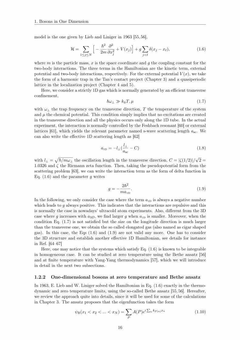
2, with c the sound velocity. The symbols are the Yang-Yang solution. Different curves are results from various theories: Sommerfield expansionof the ideal Fermi gas (IFG) and Hartree-Fock (HF) theory, Bogoliubov theory(BG), virialideal Fermi gas (virial IFG) and virial Gross-Pitaevskii (GP) predictions and LuttingerLiquid theory. This plot is from Ref. [69].
With the solution of ε(k), one can calculate thermodynamic quantities such as thegrand potential density,
Ω(µ, g, T ) = −kBT2π
∫ +∞
−∞dq ln
[1 + e
− ε(q)kBT
]. (1.36)
From the expression of Ω, we can calculate the density of the system using the thermody-namic relation
n = −∂Ω
∂µ
∣∣∣∣∣T,g
. (1.37)
One should notice that this equation is nothing but the equation of state. One example forthe application of the Yang-Yang thermodynamics is presented in Ref. [69]. One of the mainresults is concluded in Fig. 1.4. In this paper, they use the Yang-Yang thermodynamicsto calculate the difference of the chemical potential with the zero temperature solutionµLL (µ calculated from the Luttinger liquid theory, see detailed discussion in subsection1.2.4), i.e. ∆µ = µ− µLL at different temperature. Also, they calculate the correspondingsound velocity c and plot ∆µ/µLL as a function of rescaled temperature T = kBT/mc
2
under different interactions, see symbols in Fig. 1.4. In the low temperature limit, we findthe YY solution fits well with the Sommerfield expansion in the strong interaction regimewhich is expected for the fermionized bosons. In the weakly interacting regime, they alsofit well with the Bogoliubov theory. At high temperature, we find the results fit well withthe virial ideal Fermi gas and virial Gross-Pitaevskii (GP) prediction in the strong andweak interaction regimes correspondingly. Another example for application of the Yang-Yang thermodynamics is the computation of the Tan contact, which we will study in detailin Chapter 3. In that chapter, we will also take advantage of the Yang-Yang results toanalysis the different regimes of degeneracy for Lieb-Liniger bosons in harmonic trap atfinite temperature.
Quasi-condensate
For 1D bosons in homogeneous systems, it is well known that there is no condensationat any temperature. At sufficiently low temperature, the density fluctuations are sup-pressed but the phase fluctuations are not, which is the signature of a quasi-condensate.
21
1. Bosons in One Dimension
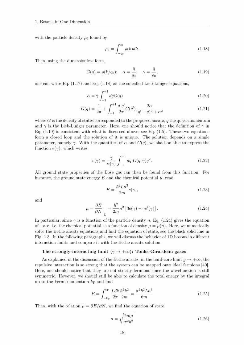
Figure 1.5: The regimes of degeneracy for 1D trapped bosons at finite temperature withthe harmonic trap α = 10. This plot is from Ref. [70].
However, at finite temperature, a true BEC may exist with a finite size system, such asthe harmonically trapped system. In Ref. [70], D. Petrov et al have given the regime ofdegeneracy for 1D bosons at finite temperature, see Fig. 1.5. The diagram is plotted inpresence of a certain harmonic trap α = 10, where α defined by
α =mgaho~2
(1.38)
with aho =√~/mω the oscillation length and ω the frequency of the harmonic trap. For
this system, there are two relevant temperatures. One is the degeneracy temperature TD
below which the system shows quantum properties, i.e. Thomas-Fermi gases in weakly-interacting regimes and fermionized bosons in strongly-interacting regime. Another one isthe coherence temperature Tφ = ~ωTD/µ In the Thomas-Fermi regime, it is always muchsmaller than TD. For T < Tφ, both the density and phase fluctuations are negligible. Inthis case, we have the true condensate, see the left up corner in Fig. 1.5. Then, whenTφ < T < TD, the density fluctuations are still negligible but the phase fluctuations arevisible. In the considered regime, the density profile is still Thomas Fermi kind but thephase coherence length extracted from the correlation function is smaller than the size ofthe system. This is what is referred as quasi-condensate in the plot. Finally, we have theTonks gas in strong interaction limit N α2 and the classical gas at high temperatureT > TD.
1.2.4 The field description: Luttinger liquid theory
Beyond the particle picture described in the last section, it’s also possible to use thefield operator to describe the system, which is known as the Tomonaga-Luttinger liquidtheory [2, 71]. At low temperature, the 1D bosonic models exhibits a liquid phase whereno continuous or discrete symmetry is broken. To be more precise, the model satisfies twomain features: (i) the low energy excitations are collective modes with linear dispersion,(ii) at zero temperature, the correlation function shows an algebraic decay with exponentsrelated to the parameters of the model. These two features define a universality class of1D interacting bosonic systems which is known as the Tomonaga-Luttinger liquids [2, 71].
The collective nature of the low-energy excitations in 1D can be easily understood bythe special space structure in 1D. Thanks to the existence of interaction, a particle hasto push its neighbour while it is moving. Thus, when a particle is moving in a certain
22

1. Bosons in One Dimension
direction, the individual motion will quickly be converted into a collective one. This canbe fruitfully described by a field description [2, 72]. The boson field operator normallywrites
Ψ† = [ρ(x)]1/2e−iθ(x) (1.39)
where the two collective fields are the density ρ(x) and the phase θ(x). Here, the twooperators satisfy the commutation rule,
[ρ(x), θ(x′)] = iδ(x− x′). (1.40)
Considering a translationally invariant system, the ground state has a constant averagedensity ρ0. The full expression of the density operator writes [72]
ρ(x) '(ρ0 −
1
π∂xφ(x)
) +∞∑j=−∞
aje2ij(πρ0x−φ(x)), (1.41)
with φ(x) a slowly varying quantum field. Here, all the oscillating term are included in theexpression. To write the Hamiltonian under the field description, we can rewrite Eq. (1.6)as
H =
∫dx
(∇Ψ†∇Ψ
2m+g
2Ψ†Ψ†ΨΨ
)(1.42)
To proceed further, we will do two approximations: (i) We assume the field φ(x) is smoothon the scale of ρ−1
0 , thus the high order oscillating term in Eq (1.42) will vanish whenperforming the integral on x. (ii) We consider low enough temperature where the exci-tation satisfied the linear dispersion, thus the value k is small enough and we can ignorethe high order term of k, i.e. the term (∇2φ(x))2. More details of the derivations canbe found in Refs. [2, 3]. Finally, with the two approximations mentioned above, we cancombine Eq (1.42), Eq (1.39) and Eq (1.41), and write the effective Hamiltonian in thefield representation
H =~
2π
∫dx
(cK
(∂θ
∂x
)2
+c
K
(∂φ
∂x
)2)
(1.43)
where c is the sound velocity which leads to the linear dispersion ω = c|k|. And K is theso-called Luttinger parameter which describes the relative weights of the phase and densityterms in Eq. (1.43). Arguably, the most remarkable feature of Luttinger liquids is that thecorrelation functions all decay algebraically. While c sets the velocity scale, the parameterK describes universal features. For instance, for the one-body correlation function g1(x),one can show that it decays as
g1(x) ∝(
1
x
)1/2K
(1.44)
with the exponent related with K. Here, the algebraic decay of the correlation functionsis a pivotal characteristics of Luttinger liquids. Also, one should notice that this approachis called harmonic fluid approach (also called "bosonization").
1.3 One-dimensional bosons in a lattice
In the previous section, we have considered the 1D bosons in a continuous system. Now, weturn to the case with the presence of a lattice, i.e. for the Hamiltonian Eq. (1.6) with theexternal potential V (x) = V0cos(kx) with V0 the amplitude of the lattice. We start withthe deep lattice case, where we have the tight-binding Bose-Hubbard model. Then, wemove to the more general case, where the problem can be solved either by the Sine-Gordonmodel analytically, or by the numerical Monte Carlo calculation.
23

1. Bosons in One Dimension
Figure 1.6: Mott transition in 3D Bose-Hubbard model, plot from Ref. [1]. (a). Schematiczero-temperature phase diagram of the 3D Bose-Hubbard model. Dashed lines of constant-integer density n = 1, 2, 3 in the SF hit the corresponding MI phases at the tips of the lobesat a critical value of J/U , which decreases with increasing density n. Here, the system isjust holding by optical lattices without an harmonic trap. (b). The wedding cake modelwhich presents the phase distribution of cold atoms in optical lattices with a harmonictrap. The starting point of the red arrow is the bottom of the trap. With the direction ofthe red arrow, the trap potential increases, which decreases the effective chemical potentialµ(r) = µ0 − Vtrap(r), creates several SF and MI regions.
1.3.1 One-dimensional Bose-Hubbard model
In the deep lattice limit, i.e. V0 is the largest energy scale in the problem, we can usethe tight-binding approximation and the eigenstate Ψ(x) could be written in the basis ofthe Wannier function. Here, the meaning of the "large enough" lattice amplitude can betranslated into two main points: (i) both the thermal and mean interaction energies at thesingle site are much smaller than the energy separating the ground Bloch band from thefirst excited band. It means Ψ has no component on the excited band. (ii) the Wannierfunction decay essentially within a single lattice site, which means only on-site interactionsare taken into account. Under these assumptions, we can write the Bose-Hubbard (BH)model in one dimension
H =∑j
[− J
(b†j bj+1 + H.c.
)+U
2b†j b†j bj bj − µni
](1.45)
where j is the index of the lattice site, b†j and bj are the bosonic creation and annihilationoperators on lattice site j, and ni = b†j bj is the site occupation operator. The pre-factorof the three terms are the tunneling J , interaction strength U and chemical potential µ.For cold atom systems, it’s possible to compute the term J and U from first principles, seedetails in Ref. [1, 42]. The main interest of studying the BH model is the Mott transition,i.e. the transition between a compressible conducting phase named superfluid (SF) and anincompressible insulator phase named Mott insulator (MI).
Mott transition in the three-dimensional Bose-Hubbard model
We start with the phase diagram of SF-MI transition in 3D, and then moving to thecase of 1D by comparing their similarities and differences. In 3D,D. Jaksch et al. firstlypropose to study the SF-MI transition in cold atom systems theoretically in 1998 [42].
24

1. Bosons in One Dimension
Figure 1.7: Absorption images of multiple matter-wave interference patterns after atomswere released from an optical lattice potential with a potential depth of (a) 0Er, (b) 3Er,(c) 7Er, (d) 10Er, (e) 13Er, (f) 14Er, (g) 16Er, and (h) 20Er. The ballistic expansion timewas 15 ms. The interference pattern visible on panels (a) of the SF phase. In contrast,absence of interference signals the MI phase. This figure is from Ref. [43].
The theoretical phase diagram is plotted in Fig. 1.6. Figure 1.6(a) describes the phasediagram of the 3D BH model without an additional trap. In this diagram, the black solidline notes the transition points of the two phases. On the left side of the line, there existsseveral MI phases with integer atom number per lattice site. On the right side, there isthe region of the SF phase where the atom number in each lattice site fluctuates, whichcan be associated with inter-site phase coherence. Following the red array, which scansthe chemical potential with the fixed interactions, there exists several transitions betweenSF and MI. In the presence of a harmonic trap, the red arrow could be probed. Shown asFig. 1.6(b), the phase distribution of the cold atoms in optical lattices with an additionalharmonic trap Vtrap(r) = mω2r2/2 is depicted. Here, the starting point of the red arrowis the bottom of the trap. Following the red arrows, the trap potential increases, whichdecreases the "local chemical potential" µ(r) = µ0 − Vtrap(r), and induces several phasetransitions between MI and SF. In the red arrow of Fig. 1.6(b), the interaction U andtunneling J is fixed while µ(r) vanishes. Therefore, it equally corresponds to the red arrowin Fig. 1.6(a).
The first experimental observation of the Mott transition in 3D BH model was firstdone by M. Greiner et al. in 2002 [43]. In the experiment, they prepare a cold atom gasin a 3D optical lattice in the presence of the harmonic trap. They observe the transitionphenomenon by scanning J/U while the atom number is approximately fixed. In theirsetup, they fixed the scattering length and scanned the parameter J/U by changing thelattice depth. The lattice depth is noted by the unit of the recoil energy Er = 2k2/2m,which is a natural measure of energy scales in optical lattice potential. Under the scanning,the system enters the MI phase from the SF phase. Figure 1.7 shows the absorptionimages of the matter wave interference in the experiment which draws the phase transitionbetween SF and MI. For small lattice depth, because of the coherence of SF phase, severalinterference peaks appear after an expansion period. On the opposite, when the latticedepth is large, the system reaches the MI region. Without any interference, the expansionpicture shows a single Gaussian-like distribution, which is characteristic of localization ofbosons in single sites. Therefore, from Figure 1.7(a) to Figure 1.7(h), with the increasingof the lattice depth, the phase transition from SF to MI is observed.
25

1. Bosons in One Dimension
Figure 1.8: Phase diagram of 1D BH model at zero temperature. (a). Phase diagram atthe region nearby the first MI lobes presented in Ref. [3]. It contains different set of resultsfrom different methods: quantumMonte Carlo results ( "+" from Ref. [73] and "x" fromRef. [74]) , earlier DMRG results (filled circle from Ref. [75]), later DMRG results (emptyboxes from Ref. [76]), and analysis of 12-th order strong-coupling expansions (solid linefrom Ref. [77]). (b). Schematic phase diagram of 1D BH model on a larger range of thechemical potential µ, from Ref. [36].
Mott transition in one-dimensional Bose-Hubbard model
Qualitatively, the SF-MI phase transition in optical lattices is similar in all dimensions.However, in one dimension, there are two main features which are different from the caseof 3D. First, different from 3D, for arbitrary low potential amplitude, there always existsMott insulator phase in the 1D lattice model. We will discuss this point in detail in thenext subsection. Another main difference is the sharp tip structure of the Mott lobes. InFig. 1.8, we show the phase diagram of the 1D BH model. In Fig. 1.8. (a), we show thephase diagram in the region of the first Mott lobe n = 1 from Ref. [3]. Here, the term tis the tunneling term which is equivalent to our parameter J , The plot consists of datasfrom different methods of calculations [73–77], see details in the caption. It indicates asharp tip structure of the Mott lobe totally different from the 3D case. Moreover, in thedifferent calculations, they both find the critical value (J/U)c on the tip nearby 0.3 withabout 3% variation. In Fig. 1.8. (b), we show a schematic phase diagram on a larger rangeof µ from Ref. [36]. The scale of the diagram is comparable with Fig. 1.6(a) and one canclearly see the difference on the shape of the Mott lobes. Moreover, this plot also helps usto distinguish two main types of the phase transition in 1D:
• Mott-U transition (dashed pink and red line): Fix the fillings n and increasing thevalue of J/U , one cross from the MI phase to SF phase via the tip of the Mott lobe.This transition is of the Berezinskii-Kosterlitz-Thouless (BKT) type.
• Mott-δ transition (vertical dashed line): fixing the value of J/U and varying thechemical potential µ. The system crosses between a MI phase with commensuratefilling and a SF phase with incommensurate filling. The transition is of Prokfovsky-Talapov type [3, 78] and is also called commensurate-incommensurate transition.
Here, one may notice that for the Luttinger parameter K which depicts the algebraic decayof the correlation function, it is finite in the SF phase and zero in the MI phase. In fact,the Luttinger liquid is valid in the SF phase. The MI phase is signalled by an instabilityand the Luttinger liquid description actually breaks down. For a commensurate order p, ithas been shown that the critical values of K are Kc = 1/p2 and Kc = 2/p2 for the Mott-δand Mott-U transition correspondingly, see details in Refs. [79–81].
26

1. Bosons in One Dimension
Figure 1.9: Modulation spectroscopy on bosons in shallow and deep optical lattices.(a),(b),(d) are the spectra for low(a), intermediate(b) and high(d) lattice depth V , whichdepicts the δ − f dependence. (c) shows the determination of the transition point for thecase of the shallow lattice depth V = 1.5Er. The diagram is from Ref. [13].
1.3.2 One-dimensional bosons in shallow periodic lattice
For the case of 1D shallow periodic lattices, the BH model is not effective anymore. Thus,we need a more general model or more powerful computation method for studying thephase diagram.
The Sine-Gordon model
To describe the 1D Bose gases in a shallow periodic potential, one proper way is theSine-Gordon (SG) model [71]. It is the Luttinger Hamiltonian Eq. (1.43) complemented bya cosine term, which accounts for the shallow periodic potential. Note, however, that theamplitude V is not the bare amplitude of the potential because of the renormalization ofthe amplitude in the heuristic Hamiltonian. In the Sine-Gordon model, the Hamiltonianwrites [13]
H =~c2π
∫dx
(K
(∂θ
∂x
)2
+1
K
(∂φ
∂x
)2
+V nπ
~ccos(2φ)
)(1.46)
with V the amplitude of the lattice and n the particle density. Based on this model, it’spossible to perform analysis and compute the important quantities such as the transitionpoint and critical Luttinger parameters, see details in Refs. [2, 3].
The first experiment studying the 1D Mott transition in a shallow lattice was reportedin Ref. [13]. Using a deep 3D lattice, they create the 3D ultracold gases in Mott-Hubbardstate with one atom per lattice site. Reducing the lattice depth in one direction, they
27

1. Bosons in One Dimension
Figure 1.10: Phase diagram of 1D strongly-interacting bosons from Ref. [13]. The twoparameters for the phase diagram are the inverse Lieb-Liniger parameter 1/γ and thelattice depth V in the unit of the recoil energy Er. The inset shows the measured gapenergy Eg as a function of V .
obtain arrays of 1D tubes in the presence of a periodic potential on the transverse direction.The phase of the system can be probed with the amplitude modulation spectroscopy, whichdetects the excitation gap and distinguish the gapped Mott insulator phase from the gaplesssuperfluid phase. Firstly, they induce a modulation to the frequency f of the potentialof the system. Then, they ramp down the lattice beams, give the system a suspendedexpansion of 40 − 60ms, detect the atoms from time-of-flight, and determine the atomicspatial width δ by a Gaussian fit. By plotting the δ−f relation and studying the slope, onecan obtain the information of the energy gap. The experimental results for different latticedepths are shown in Fig. 1.9(a),(b),(d). For shallow lattices in the strong interaction regime(blue circles), there is a sudden change in the slope which can be associated to the existenceof an excitation gap and it is attributed to the signature of Mott insulator. In contrast, inthe weak interaction regime (red square), the δ − f relation presents a linear dependencewhich reflects the gapless superfluid character of the gas. Similar interpretation can betaken out for the two cases of larger lattice depths, see Fig. 1.9(b) and (d). However,one may notice that the difference between Fig. 1.9(a) and Fig. 1.9(d) gives an obviouscomparison to the two limit sides of the model, Sine-Gordon model and BHM model.
To further locate the transition point, one find the intercept of the linear fit with theaxis of the curve in Fig. 1.9(a) and (b) which gives the frequency gap fg. By scanningthe Lieb-Liniger parameter γ, the diagram of the fg − γ is depicted in Fig. 1.9(c) (aswell as its inset), which gives the transition point between SF and MI phase for a fixed,shallow potential. In the case of a deep lattice, the state of the system is determined by thetransport measurement which is more sensitive in this regime. With all the results measureabove, they plots the phase diagram for the 1D strongly-interacting bosons, see Fig. 1.10.The transition points are determined either by amplitude modulation spectroscopy (redcircles) in the shallow lattice regime, or by transport measurement (blue squares) in thedeep lattices regime. The solid and dashed lines are predictions from SG and BH models,which fit well with the experimental data within errorbars, respectively. Also, the value γcin the limit V = 0 fits with the predicted value γc = 3.5 in Ref. [82]. However, one maynotice the significant errobars on the shallow lattice data points, which did not allow todraw an accurate phase diagram. Also, for the phase transition of an intermediate valueof the potential amplitude, a powerful numerical technique is needed.
28

1. Bosons in One Dimension
Figure 1.11: (a). Phase diagram in the g-V plane at the commensurate filling na = 1. Thebig black and small green points are QMC theoretical and experimental results. The solidblue line is the BHM prediction and the red dashed line is the result from bare sine-Gordontheory. (b). The critical momentum pc versus 3D scattering length a3D for different latticedepths: V/Er = 1 (red), 2 (orange), 2.8 (green), 4 (blue). The inset is one example for thetime evolution of the momentum distribution peak p for a3D = 109a0 and V/Er = 2. Thediagram is from Ref. [15].
The continuous space QMC
To determine the Mott transition point accurately at any values of lattice strength, oneneeds to seek for powerful numerical tools. The quantum Monte Carlo (QMC) method incontinuous space appears to be a solution to this problem (see details about the techniquein Chapter 2). From the QMC calculation, one can calculate the superfluid fraction fs,compressibility κ and Luttinger parameter K. All these three quantities are finite forsuperfluid (compressible conductance) phase, but zero for Mott insulator (incompressibleinsulator) phase. From these data, one can locate the Mott transition accurately. In 2016,G. Boéris et al have performed such kind of calculation in Ref. [15]. The main results areshown in Fig. 1.11. In Fig. 1.11 (a), the black dots are the QMC solution. Different fromthe BH model (blue line) and the Sine-Gordon model (red line) mentioned above, thiscalculation has no range limitation of the lattice depth and the interaction strength, for ituses the continous space Lieb-Liniger Hamiltonian Eq. (1.6) without any approximation forthe lattice potential V (x) = V sin2(kx). Based on this Hamiltonian, with the appropriateQMC calculations, the transition curve could be accurately determined in both the shallowand deep lattice regimes. For small γ, the QMC data (black dot) fits well with the BHmodels (light-blue solid line). However, for large γ, the QMC data separate from the SGmodel (red dashed line), although they reach the same limit at V = 0. In fact, the SGis applicable but the lattice, even weak, significantly renormalize the Luttinger parameterwhich explains the deviation to the SG prediction with no renormalization (red dashedline).
An experimental measurement is also presented in the same reference. In the experi-ment, they start with the 3D Bose-Einstein condensate of 39K atoms. With 2D horizontaloptical lattice, they create 1000 vertical 1D tubes. By varying the 3D scattering lengtha3D, they can tune the Lieb-Liniger parameter γ in the range 0.07 − 7.4. In most of thetubes, they control the fillings na = 1. To detect the quantum phase, they suddenly switchoff the magnetic field gradient which provides a shift of the potential and drags the sys-tem. After the atoms evolve in a time duration t, they switch off all the optical potentialsand record the time-of-flight images, especially the momentum distribution peak p. Oneexample of the function p(t) is shown as the black dots in the inset of Fig. 1.11 (b). Wecan see that p(t) increases up to a critical value pc. By detecting the value pc while varying
29

1. Bosons in One Dimension
Figure 1.12: Phase diagram in the g − µ plane from QMC calculations at the potentialV = 2Er. There exists two quantum phases: the superfluid(white) and Mott insulator(red). The black points joined by lines are the phase transition points. The blue dashedlines are the prediction from the BH model. In the inset, there are the detailed plotsfor the four parameters computed from the QMC, namely the particle density n, thecompressibility κ, the superfluid fraction fs and the Luttinger parameter K. These dataare at the interaction g = 7~2/ma and various system sizes L/a = 30, 50, 100 (blue, greenand red).
a3D, we know that it should show strong dependence in the SF phase and remain constantin the MI phase, see several examples in the main plot of Fig. 1.11 (b). Here, one shouldnotice that pc should be zero for MI phase, however, some tubes are supefluid so that pcshows a plateau instead of strictly vanishing. From this scan, one can get the transitionpoint at different potential amplitude V , see green points in Fig. 1.11 (a). Here, we findthat it is in good agreement with the theoretical results.
One main interesting outcome from this calculation is that the curve hits the 1/γ axisat the red cross point, which means that for an arbitrary small amplitude of the latticepotential, there always exists a Mott insulator phase. This is totally different from the3D case, where below a critical lattice potential amplitude Vc, no MI phase is found. Thisspecial property of 1D bosons may be attributed to the specificity of the Tonks-Girardeaulimit. In this limit, the Mott lobes can be mapped onto the band gap of ideal fermionsin a lattice, which exists at any nonvanishing potential amplitude. Thus, it will form aincompressible insulator states.
Also, in this paper, the authors perform the QMC calculations for a fixed potentialamplitude V = 2Er with various interaction g and chemical potential µ, see Fig. 1.12. Inthe plot, the black points joined by lines are the transition points determined by the QMCdata. One example of which is shown in the inset plot. In the inset, they present the QMCdata for the particle density n, the compressibility κ, the superfluid fraction fs and theLuttinger parameter K at g = 7~2/ma and various system sizes L/a = 30, 50, 100 (blue,green and red). By increasing the sizes, one finds that the transition gets sharper andsharper. Finally, by finding the position κ = κc = 0, fs = fsc = 0 and K = Kc = 1, theydetermine the transition points in the main plot (see inset of Fig. 1.12). There, surroundedby a superfluid region (white), they find the Mott lobes na = 1 (red) significantly differentfrom the BH prediction. However, they still find the sharp tip structure of the Mott lobeswhich is different from the 3D case.
30

1. Bosons in One Dimension
Figure 1.13: Phase diagrams of 1D bosons in disordered potentials at zero temperature. Ineach plots, the x-axis is the interaction strength and the y-axis is the disorder amplitude.(a). 1D bosons in continuum, calculated from renormalization group techniques. K isthe Luttinger parameter and D is the disorder strength. The solid red line is the SF-BG transition calculated from RG calculations, which leads to Kc = 3/2 in the limitof zero disorder. The dashed blue line is still open. On the left side, the blue verticalline indicates the Anderson localization phase at zero interaction. This subfigure is fromRef. [3]. (b) and (c) are phase diagrams for 1D Bose-Hubbard model with the on-site energyfollows a uniform random distribution in the range [−∆,∆], calculated from density-matrixrenormalization group (DMRG), with incommensurate filling n = 0.5 and commensuratefilling n = 1. These two subfigures are from Ref. [83].
1.3.3 One-dimensional bosons in purely-disordered potentials
The interacting bosons in the presence of a disordered potential, known as the dirty bosonproblem, is one of the interesting topics on understanding the nature of quantum phases.
At zero temperature, the case of 1D Bose-Hubbard model with incommensurate fillingsis similar to the continuous gases, in the presence of disorder. The Hamiltonian of thedisordered Bose-Hubbard model writes
H =∑j
[− J
(b†j bj+1 + H.c.
)+U
2b†j b†j bj bj − Vj b
†j bj
](1.47)
with Vj the random onsite energy. The phase diagram of such kinds of systems was firstproposed in Ref [52]. The calculations were performed by bosonization and renormalizationgroup (RG) techniques, where they treated the disorder as a perturbation. The resultsare shown in Fig. 1.13(a). Here, they find two phases: a compressible superfluid, anda incompressible insulator named Bose glass (BG). Different from the Mott insulator wementioned before, the BG phase is gapless since the insulating property is induced bydisorder. For the case of ideal gas (K = ∞), all the particles stay on the ground statewhich forms the Anderson localization. For finite but small interactions, more states arepopulated although the system remains insulating. In the intermediate interaction regime,when the disorder D is low enough, the conducting islands in the system connect with eachother and the system becomes a superfluid. Further increasing the interaction, the bosonsare pinned by the disordered potential and the superfluidity is destroyed again. In thestrong interaction regime, the phase transition point are determined precisely in Ref [52],see red solid line in Fig. 1.13(a). They are found as BKT type and the critical Luttingerparameter hits Kc = 3/2 in the limit D = 0. On the contrary, the perturbative RG failsin the weak interaction regime, which is shown as the blue dashed line in Fig. 1.13(a).This part is further studied by numerics in Refs. [22, 83, 84]. In Ref. [83], the phasediagram of 1D BH model with incommensurate filling n = 0.5 is obtained by density matrixrenormalization group (DMRG), see Fig. 1.13(b). This further confirms the structure
31

1. Bosons in One Dimension
predicted in Fig. 1.13(a).The case of 1D Bose-Hubbard model with commensurate fillings is slightly different. In
the absence of disorder (D = 0), we already know from section 1.2.1 that a Mott insulatorappears in the strongly-interacting regime. The phase diagram for this case was firstlyproposed by Ref. [54] (see detailed discussion in Sec. 5.1.1). Then, a numerical study wasperformed in Ref. [83], see Fig. 1.13(c). As we expected, a Mott insulator was found in thestrongly-interacting regime where the disorder is weak. Also, as argued by Ref. [54], theMI phase is totally surrounded by BG, which equivalently means that there is no directtransition from MI to SF. It has been shown to be correct even in higher dimension, seeRef [85].
In recent years, the case of a quasiperiodic potential, which is the intermediate betweenthe periodic and disordered potentials, has drawn people’s attention. Obtaining the phasediagram and study the phase transitions between the SF, MI and BG phases have becomeone of the main interesting questions to address. In Chapters 4 and 5 of this manuscript, wewill introduce the question of quasiperiodic systems and study in detail its phase diagrams.
Conclusion and Outlook
1D bosons are special. In this chapter, we went through the basic knowledge of 1Dbosons and some of the main aspect we shall build on in this thesis. We started withthe general interest of the 1D bosonic systems, especially indicating its special propertieswhich are totally different from 3D. Then, we introduced the basic concept for 1D contin-uous bosonic systems. We introduced the two main approaches for describing such kindof systems: the particle description Lieb-Liniger model and the field operator descriptionLuttinger liquid model. Finally, we turn to the introduction of 1D bosons in the pres-ence of an optical lattices, be it deep or shallow. We introduced several theoretical andexperimental studies on the superfluid-Mott insulator transition.
Beyond the introduction we presented here, there are still many open questions to beinvestigates for 1D bosonic systems. These properties forms the basis on which we shallbuild in the thesis. On the one hand, we shall study the Tan contact in harmonicallytrapped Lieb-Liniger gases at arbitrary temperature, which is a central characteristics ofinteracting systems (Chap. 3). On the other hand we shall study localization propertiesin quasiperiodic potentials, extends the Mott transition in a shallow periodic potential(Chaps 4 and 5)
32

Chapter 2
Continuous-space quantum MonteCarlo for bosons
Schordinger equation is known to provide a correct description of any quantum system.However, for most of the cases of many-body problems, it is a tremendous challenge to cal-culate exactly the physical quantities from it, due to the exponential growth of the Hilbertspace dimension with the number of particles. To solve this problem, physicists have ex-plored plenty of methods dedicated to certain kinds of Hamiltonian, both analytically andnumerically, over the last decades.
For a few Hamiltonians, the equation can be solved analytically. In 1D, see for in-stance the examples in section 1.2. Beyond those, numerical methods are necessary toan efficient calculation of the solution. For example, exact diagonalization works prop-erly for single particle problem in various inhomogeneous potentials [31, 86], or for thelattice spin systems with a couple of tens of spins [87, 88]. For the Ising model, one canuse mean-field approximation in high dimensions to obtain reliable results. In the case ofweakly-interacting boson systems, the property could be described properly by the Gross-Pietaevskii equation and Bogoliubov theory [89–91]. However, all those techniques fail forstrongly-interacting problems.
QuantumMonte Carlo (QMC) approaches can overcome the difficulty in certain cases. [92]The Monte Carlo approaches contains a large variety of different types and each of themhas its pros and cons. The variational Monte Carlo (VMC) applies the variational methodsto compute the ground states properties [93,94]. The method is simple but the accuracy ofthe results depend crucially on the trial wavefunction. The diffusive Monte Carlo (DMC)method generalizes DMC by working with complex wavefunctions and it calculates betterthe ground state properties by avoiding the systematic errors [95, 96]. To compute thefinite-temperature properties, however, one needs to call for more powerful techniques, forinstance the path intergral Monte Carlo (PIMC). This method was first introduced byCerperley and Pollock [97–99], and it provides a first quantitative result for the Helium4 superfluid transition. In this manuscript, the QMC we used is PIMC, since it solvesperfectly the properties of ultracold bosonic systems in various inhomogeneous externalpotentials, at any regime of interaction and temperature. It fits well with the subject westudy. Nevertheless, despite the method is powerful for the system we are interested, wehave to point out that the extension of the PIMC to fermionic systems and time-dependproblem is extremely difficult. There are other Monte Carlo methods which may overcomethose problems in certain cases. For instance, bold diagrammatic Monte Carlo which alle-viate the sign problem for fermions [100]. And time-dependent Monte Carlo which opensthe way for the study of dynamics [101,102].
In this Chapter, we first briefly introduce the path integral Monte Carlo in continuousspace, which is the QMC method we used widely in our simulation. We shall describe
33

2. Continuous-space quantum Monte Carlo for Bosons
the basic PIMC as introduced in the pioneering work of Cerperley and Pollock [97–99].Then, we present the building blocks of Monte Carlo methods, namely the basic moveswith the so-called worm algorithm. It is first developed by Prokov’ev and Svistunov [58,59], which improved strongly the computation efficiency for certain variables such as thesuperfluid fraction. Finally, we briefly describe how we compute the the physically-relevantobservables in detail, which is the final goal of the QMC calculation.
2.1 Path-integral Monte Carlo for interacting bosons
In this section, we present the PIMC method for interacting bosons at finite temperature asin [97,99]. There are two main ideas of the PIMC. First, using the Feynman path integralrepresentation, one can map the quantum systems with interacting particles onto a classicalsystem with interacting polymers. Then, we sample the partition function of such a systemstochastically using the Monte Carlo approach. Finally, we obtain the targeted observablesby the averaging values over the generated polymer configurations.
2.1.1 Feynman path integral for a single particle
Quantum mechanics, formulated by Dirac, Heisenberg, and Hilbert in 1920s, depicts thephysical states of a system by vectors in a Hilbert space. The time evolution of such astate is controlled by the operator called Hamiltonian. Thanks to the "canonical quantiza-tion", classical quantities such as the position, the momentum, and the Hamiltonian, arepromoted to operators satisfying certain commmutation relations.
The path integral approach is another formulation. It formulates quantum mechanics insuch a way to recover the least action principle in the classical limit (h→ 0). The essentialidea was first presented in the works of Wiener and Dirac [103–105], and formalized byFeynman [106]. The later has also proved that it’s equivalence with standard quantummechanics. Here, we start with the path integral formulation of a single particle, which isthe conceptual basis of the PIMC.
Imaginary time path integral for a single particle
Considering a single particle evolving in a d-dimensional space, its Hamiltonian readsas
H = H0 + V (r) (2.1)
with H0 = p2
2m the kinetic term, p = −i~∇ the momentum operator, m the particle massand V the external potential. The main quantity of interest is the propagation amplitude〈rf |e−τH |ri〉 between the initial and final points ri and rf . If τ is a purely imaginarynumber, this quantity stands for the probability amplitude for the particle to propagatefrom ri to rf during the real time τ = it/~, under the Hamiltonian H. In the following, wecall τ the imaginary time, although it has the dimension of an inverse energy. Normally, thisexponential term is difficult to be computed directly, since the kinetic and potential termin the Hamiltonian do not commute. To overcome this difficulty, we split the propagatorinto J pieces in the imaginary time, with each piece a shorter time propagator in a timeinterval ε = τ/J . Introducing the identity operator I =
∫dr|r〉〈r| between each ε step, it
writes〈rf |e−τH |ri〉 =
∫drJ−1...dr1 〈rf |e−εH |rJ−1〉 × ...× 〈r1|e−εH |ri〉. (2.2)
Using the primitive approximation e−ε(A+B) = e−εAe−εB +O(ε2), we can write the short-time propagator as
〈r′|e−εH |r〉 = 〈r′|e−εH0 |r〉e−εV (r) +O(ε2). (2.3)
34
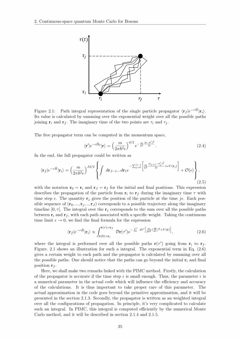
2. Continuous-space quantum Monte Carlo for Bosons
Figure 2.1: Path integral representation of the single particle propagator 〈rf |e−τH |ri〉.Its value is calculated by summing over the exponential weight over all the possible pathsjoining ri and rf . The imaginary time of the two points are τi and τj .
The free propagator term can be computed in the momentum space,
〈r′|e−εH0 |r〉 =( m
2π~2ε
)d/2e−
m~2
(r−r′)22ε . (2.4)
In the end, the full propagator could be written as
〈rf |e−τH |ri〉 =( m
2π~2ε
)Jd/2∫
drJ−1...dr1e−
∑J−1j=0
[m~2
(rj+1−r′j)2
2ε+εV (rj)
]+O(ε)
.
(2.5)with the notation r0 = ri and rJ = rf for the initial and final positions. This expressiondescribes the propagation of the particle from ri to rf during the imaginary time τ withtime step ε. The quantity rj gives the position of the particle at the time jε. Each pos-sible sequence of (r0, ..., rj , .., rJ) corresponds to a possible trajectory along the imaginarytimeline [0, τ ]. The integral over the rj corresponds to the sum over all the possible pathsbetween ri and rf , with each path associated with a specific weight. Taking the continuoustime limit ε→ 0, we find the final formula for the expression
〈rf |e−τH |ri〉 ∝∫ r(τ)=rf
r(0)=riDr(τ ′)e−
∫ τ0 dτ ′
[m2~2 ( dr
dτ)2+V (r)
], (2.6)
where the integral is performed over all the possible paths r(τ ′) going from ri to rf .Figure. 2.1 shows an illustration for such a integral. The exponential term in Eq. (2.6)gives a certain weight to each path and the propagator is calculated by summing over allthe possible paths. One should notice that the paths can go beyond the initial ri and finalposition rf .
Here, we shall make two remarks linked with the PIMC method. Firstly, the calculationof the propagator is accurate if the time step ε is small enough. Thus, the parameter ε isa numerical parameter in the actual code which will influence the efficiency and accuracyof the calculations. It is thus important to take proper care of this parameter. Theactual approximation in the code goes beyond the primitive approximation, and it will bepresented in the section 2.1.3. Secondly, the propagator is written as an weighted integralover all the configurations of propagation. In principle, it’s very complicated to calculatesuch an integral. In PIMC, this integral is computed efficiently by the numerical MonteCarlo method, and it will be described in section 2.1.4 and 2.1.5.
35

2. Continuous-space quantum Monte Carlo for Bosons
Path integral in real time
For completeness, we provide the classical limit of the path integral formalism, whichcorresponds to the original one proposed by Dirac and Feynman. Using the correspondenceτ → it/~ with t the real time, we obtain
〈rf |e−itH/~|ri〉 ∝∫ r(t)=rf
r(0)=riDr(t′) e
i~S[r(t′], (2.7)
with S[r(t′] =∫ t′
0 [12mr2 − V (r)] is the action of the classical system. Similarly, the real-
time propagator is computed with the sum over all the possible paths with an assignedphase proportional to the classical action. In the limit ~ → 0, thanks to the stationaryphase argument, only the paths which extremize the action contribute to the integral andthe other ones are cancelled. This recovers exactly the principle of least action in classicalmechanics.
Feynman-Kac formula
In Eq. (2.7), we drop the prefactor for simplicity. However, the term could actuallyblow up in the continuous limit. To avoid this difficulty, one possibility is to divide it bythe free propagator 〈rf |e−itH0/~|ri〉. The prefactors are cancelled since they are identicalin both cases. Then, one may recognize the term
π[r(τ ′)] = e−∫ τ0 dτ ′ m
2~2 ( drdτ
)2/
∫ r(τ)=rf
r(0)=riDr(τ ′)e−
∫ τ0 dτ ′ m
2~2 ( drdτ
)2 (2.8)
is the probability density of a Brownian process with volatility σ =√~2/m. Because the
process is fixed to start and end at certain fixed point, it’s called a Brownian bridge betweenri and rj . Using the stochastic interpretation, one shall get the so-called Feynman-Kacformula [107],
〈rf |e−τH |ri〉〈rf |e−τH0 |ri〉
=
⟨exp
[−∫ τ
0dτ ′V (r(τ ′))
]⟩π
(2.9)
where < ... >π represents the expectation value under the Brownian measure Eq. 2.8. Thisformula will be useful in further calculations of the imaginary time propagator, see section2.1.3.
2.1.2 Feynman path integral for many-body bosonic systems
Now, consider a N boson system in a d-dimensional continuous space. We will derive thepath integral representation used in the PIMC algorithm. The main aim of the methodis to compute the expectation value of an observable A of interest at thermodynamicequilibrium, in the canonical ensemble at temperature T . It can be written as
〈A〉 =1
ZTr[e−βHA] (2.10)
where β = 1/kBT is the inverse temperature and Z = Tr[e−βH ] is the partition function.Here, we use the variable R = (r1, r2, ..., rN) to denote the positions of the N parti-cles. To take into account the indistinguishability of identical bosons, we introduce thesymmetrization operator
S =1
N !
∑σ∈Π
|σ ·R〉〈R| (2.11)
36

2. Continuous-space quantum Monte Carlo for Bosons
Figure 2.2: Path integral representation of the many particle propagator. The plotillustrate the configuration of N particles which enters the partition function.
where Π stands for the group of permutations of theN elements and |σ·R〉 = |rσ1 , rσ2 ..., rσN〉is one of the possible permutations of R. Therefore, the trace of an operator X should bewritten as
Tr[X] =
∫dR〈R|XS|R〉. (2.12)
Then, similarly as the single particle case, splitting the inverse temperature axis [0, β] ininfinitesimal portions of step ε = β/J with J the number of steps, we can finally write
Tr[e−βHA] =1
N !
∑σ∈Π
∫dRJ−1...dR0〈σ·R0|e−εH |RJ−1〉×...×〈R2|e−εH |R1〉×〈R1|e−εHA|R0〉.
(2.13)Here, one should notice that the expression is obtained thanks to the fact that S commuteswith H, A as well as I, and it satisfies the condition S2 = S.
In the expression Eq.( 2.13), a possible distribution (R1,R2, ...,RJ) is defined as aconfiguration C. A typical example of configuration is shown in Fig. 2.2. In the plot, eachparticle propagates along a trajectory in imaginary time from τ = 0 to β, which is called aworldline. The position of the i-th particle at time jε is called bead. It is noted as rji anddepicted as a black disk. Moreover, one should notice that the condition |RJ〉 = |σ ·R0〉due to the definition of trace, which implies β-periodicity along the imaginary time axis.It also indicates that one particle could choose to close at the initial position of anotherparticle, which fits with the particle indistinguisability. The exchange cycle reflects thequantum exchange appearing at low temperature, especially involved in the phenomenonsuch as Bose-Einstein condensation and superfluidity.
In order to simply the notation, we may introduce the weight of the configuration C,
W(C) =1
N !〈σ ·R0|e−εH |RJ−1〉 × ...× 〈R1|e−εH |R0〉 (2.14)
and the normalized weight π(C) =W(C)/Z. They satisfy the normalization∫π(C)dC = 1.
Moreover, we may define the path-integral estimator for observable A, which presents as
A(C) =〈R1|e−εHA|R0〉〈R1|e−εH |R0〉
. (2.15)
We can then write the expectation value of the obervable A as
〈A〉 =
∫π(C)A(C)dC (2.16)
37

2. Continuous-space quantum Monte Carlo for Bosons
In this formula, A(C) is the value of A we calculated associated to the configuration Cand π(C) is the corresponding statistical distribution. This expression is exact but remainshard to compute directly. Therefore, we shall introduce several extra approximation stepsin the next section.
2.1.3 The imaginary time propagator
The configuration weight,W(C), is built out of the imaginary-time many-body propagator.We may notice that it is the density matrix ρ(R′,R, ε) = 〈R′|e−εH |R〉 up to a normal-ization factor. In this subsection, we introduce several approximations to compute thepropagator in the limit ε → 0. For concreteness, we write the Hamiltonian of the typicalbosonic system with two-body interactionsH = H0 + H1 + H2, with
H0 =
N∑i=1
pi2
2m, H1 =
N∑i=1
V1(ri), H2 =∑i<j
V2(ri − rj). (2.17)
Here, the three terms in the Hamiltonian are respectively the kinetic term, the externalpotential and the two-body interactions. Then, we can write the density matrix
ρ(R′,R, ε) = ρ0(R′,R, ε)e−U(R′,R,ε), (2.18)
where ρ0 is the free density matrix associated to the Hamiltonian H0 and U is called theaction. Usually, the action could be written as U = U1 + U2, with the one-body andtwo-body interaction potential terms correspondingly.
Free density matrix
Consider only the free particle Hamiltonian H0, it is trivial that the density matrixwrites
ρ0(R′,R, ε) =N∏j=1
ρ0(r′j, rj, ε), (2.19)
where ρ0(r′j, rj, ε) = (m/2π~2ε)d/2exp(−m(r− r′)2/2~2ε) is the free density matrix for oneparticle. The free density matrix actually introduces a strong condition on the configura-tions shown in Fig. 2.2. Since the particle position evolves in imaginary time steps by aGaussian with standard deviation
√ε in the unit of ~2/m, two connected beads on a single
worldline are seperated by at most several√ε. In the limit ε → 0, the paths becomes
Brownian process with volatility√~2ε/m.
The one-body action: Trotter-Suzuki approximation
The main difficulty to calculate the action of the full Hamiltonian is the fact thatthe kinetic and potential terms of the Hamiltonian do not commute with each other ingeneral. It forbids the splitting of the exponential of the Hamiltonian into separatedexponential terms. However, for small ε, the splitting is possible thanks to the Trotter-Suzuki approximation [108,109],
e−ε(A+B) = e−12εBe−εAe−
12εB +O(ε3). (2.20)
This approximation is an improved version of the primitive approximation introduced insection 2.1.1, with the validity of higher order of ε. Then, by setting A = H0 + H2 andB = H1, one can extract the one-body potential from the propagator. Therefore, theone-body action in the propagator writes finally
U1(R,R′, ε) = ε
N∑j=1
V1(r′j) + V1(rj)
2. (2.21)
38
2. Continuous-space quantum Monte Carlo for Bosons
Then, the propagator terms for H0 + H2 will be evaluated using further assumptionsin the next part. Here, one should notice that there are other possibilities for using theTrotter-Suzuki approximation. For instance, one can split the Hamiltonian by A = H0 andB = H1 + H2, in order to obtain the free particle and potential part separately. However,the first way of separating has an advantage that one can use the standard scatteringtheory, so we insist on this method for the QMC calculations in this thesis.
The two-body action: Pair-product approximation
Now, we compute the propagator with the term A = H0 +H2. The first approximationwe use here is the pair-product approximation [110], which allows us to write the many-body density matrix as a product of two-body density matrices. This approximation issufficiently precise for dilute gases and short-range interactions, i.e. the system we studied.First of all, using the Feynman-Kac formula [99], we shall write the action
e−U2(R′,R,ε) =〈R′|e−ε(H0+H2)|R〉〈R′|e−εH0 |R〉
=
⟨∏i<j
exp
[−∫ ε
0dτV2(ri(τ)− rj(τ))
]⟩(2.22)
which average is performed over the Brownian bridges joining the two points R and R′.If we assume that
√ε and the typical potential range b are much smaller than the mean
interparticle distance n−1/d, one particular path will typically interact with at most onesingle other path. Then, the N(N -1)/2 factors on the right-hand side could be consideredto be independent. Therefore, we shall write it as,
e−U2(R′,R,ε) =∏i<j
⟨exp
[−∫ ε
0dτV2(ri(τ)− rj(τ))
]⟩(2.23)
Using the Feynman-Kac formula again, we shall get
U2(R′,R, ε) =∑i<j
u2(r′i, r′j, ri, rj, ε) (2.24)
where u2(r′i, r′j, ri, rj, ε) is the action for two interacting particles. As we mentioned in
the beginning, the derivation is performed under the assumption of a rapidly decayinginteraction potential. However, for the case of long-range interactions, it’s also guaranteedto be valid for small enough ε, although less precise. This is because in the limit ε→ 0, itreduces to the Trotter approximation.
The two-body action: Change of reference
For further simplifying the two-body matrix, we turn to work in the center of massframe. We introduce the center of mass coordinate rCM = (r1 + r2)/2, the relative coordi-nate rrel = r1 − r2, the total mass M = 2m and the reduced mass m∗ = m/2. Then, thetwo-body Hamiltonian writes
H =p2CM
2M+
ˆp2rel
2m∗+ V2(rrel). (2.25)
Thanks to the fact that the momentum operator p2CM commutes with the term rrel, the
two-body density matrix can be factorized as
〈r′1, r′2|e−εH |r1, r2〉 = 〈r′CM |e−εp2CM2M |rCM 〉〈r′rel|e
−ε
[ˆp2rel
2m∗+V2(rrel)
]|rrel〉. (2.26)
Then, dividing both sides by the free density matrix, one shall find that the two-bodyaction reduces to
u2(r′1, r′2, r1, r2, ε) = urel(r
′1 − r′2, r1 − r2, ε) = urel(r′rel, rrel, ε), (2.27)
39

2. Continuous-space quantum Monte Carlo for Bosons
with urel the action for an effective particle of mass µ in the external potential V2. Forcertain cases, this action can be calculated analytically. For instance, for the 1D deltainteraction potential H2 = g
∑j<` δ(xj − x`), i.e. the system we are interested, the two-
body action writes [111]
〈r′rel|e−ε[
ˆp2rel2µ
+V2(rrel)]|rrel〉 = 1− exp
(−µ(rrelr′rel + |rrelr′rel|)
ε~2
)×√πµε
2
g
~erfc(u)exp(u)
(2.28)with u = m ∗ (|rrel|+ |r′rel|+ gε)/
√2m ∗ ε~2 and erfc is the complementary error function.
In the actual calculations, instead of going through all pairs ri and rj , we only computethe term with |ri−rj | < rjudge and rjudge is a threshold at several
√ε. The other terms are
extremely small and can be ignored. This is consistent with the property of the short-rangeinteractions and it improves the efficiency of the calculation.
Moreover, such an analytical forms for the two-body propagator are also available fordelta range interactions at higher dimension [28, 111]. However, there are some othercases where the analytical form is not provided. In this case, one shall evaluate the valuenumerically using the procedure explained in the next paragraph.
The numerical method: Feynman-Kac formula and Matrix squaring tech-nique
When an analytical formula for the propagator is not available, for instance the Hamil-tonian contains certain types of long-range interactions, one should calculate the propaga-tor using numerical procedures. Here, we propose two possible methods to do that.
First, one can evaluate the propagator using the Feynman-Kac formula [107]. For eachconsidered pairs of r and r′, one can calculate the right-hand side of Eq. (2.9) using aMonte-Carlo approach. We can discretize the Brownian bridge by a smaller time stepη = ε/Q with Q some integer. Then, one can use the Lévy construction to sample thepath [112] and obtain the action as an average over all the generated path.
A second possible method is called matrix squaring technique [107,113]. The main issueis that evaluating the propagator with direct use of Trotter approximation on discretizationstep ε is not accurate enough. Thus, one starts with the single-density matrix M0 = e−ηA
at a higher temperature η = 2−Kε where K is a integer, i.e. a smaller resolution step.Then, we are allowed to use the Trotter approximation to separate the interaction termand we have
M0(rrel, rrel′) = eη2
[V2(rrel)+V2(rrel′ )]ρ0(rrel′ , rrel, ε). (2.29)
Then, we can generate a sequence of matrices by Mk+1 = M2k and after K iterations, we
can get the matrix at the temperature ε.
2.1.4 Sampling the configurations using the Monte Carlo approach
In the previous paragraphs, we have introduced the path-integral formulation to describethe quantum many-body system by a picture of classical statistical physics with interact-ing polymers. The thermodynamical observables are then calculated by the Eq. (2.16),with π(C) the weight Eq. (2.14) calculated by the method introduced in section 2.1.3 atsmall ε limit. However, it is still hard to evaluate the integral (2.16) over all the possibleconfigurations.
The rectangular method, which numerically calculate the value of integralsA =∫f(x)dx
by dividing the configuration space into small cells and summing the integrand on the pointsof the grids times the elementary volume of the cell, i.e. A '
∑i f(xi)dxi ,are widely used
in various calculations. However, the computing cost grows exponentially with the di-mensionality of the integrated element dx. In the integral Eq. (2.13), the dimension of
40

2. Continuous-space quantum Monte Carlo for Bosons
the configuration space is NdJ , which grows to infinitely large at small ε limit. Thus,one calls for methods beyond the rectangular one and compute the result efficiently. TheMonte Carlo approach, which samples the configurations stochastically, is one of the goodchoices for this situation. One of the key reasons for its success is that they can performimportance sampling, which means the highly probable configurations are generated muchmore than the one with low probability. On the contrary, the rectangular method treatsall the configurations equally. In this section, we first describe the Monte Carlo approachfrom the general point of view, and then move to the specific case which we are interestedin.
Monte Carlo method for calculating integrals numerically
Now, we explain the core idea about the Monte Carlo approach 1 for calculating inte-grals. Considering a real-valued function f : RD → R, we want to calculate
I =
∫RD
f(x)dx (2.30)
Now, we introduce a random variable X, which takes values in the integration space RD.The probability distribution of X is noted as π which is normalized to unity,
∫π(x)dx = 1.
We should notice that a hidden condition here is that π is strictly positive since it representsthe probability density. Then, the integral may be rewritten as
I =
∫RD
f(x)
π(x)π(x)dx = 〈I(X)〉π (2.31)
where I(X) = f(X)/π(X) is a random variable linked with X and thus the value of I canbe understood by the expectation value of (I)(X) under the probability distribution π. TheMonte Carlo approach propose to compute this integral using the law of large numbers. Thebasic idea is to generate a large number of independent samples X1, X2, ..., Xn followingthe probability density π, and to estimate the integral I by calculating the average
I =I(X1) + I(X2) + ...+ I(Xn)
n. (2.32)
In the limit n → ∞, the estimator I converges to the value of the integral almost surely.However, in actual simulation, only finite number of samples are generated. Therefore, thea statistical error I − I enters into the estimation. The error can be evaluated preciselyusing the central limit theorem (CLT). It states that a random variable I − I follows aGaussian distribution with standard deviation
εI =σI√n
(2.33)
where σI is the standard deviation of I(X). A more detailed analysis of the errorbar willbe presented at the end of this subsection.
Now, we turn back to the evaluation of the observable given by the path integralEq. (2.16). For Bosons, the weight function π(C) is always positive since W(C) is always
1The original birth of the Monte Carlo method should go back to the atomic bomb project at Los Alamosin 1946. Physicist Stanislaw Ulam, who was a member of the project, was recovering from a surgery. Tooccupy his own mind from boring, he tried to play solitaire in an IQ demanded way: calculating theprobability of winning the game. His answer is simple: play it 100 times, count the number of wins andyou will have a pretty good estimation. Thanks to the availability of the computer at the time, this methodbecame quite practical for a variety of questions, such as the mechanical simulation of random diffusionof neutrons. As a secret government work, a code name is asked. The name of the Moncaco city "MonteCarlo", is given to this approach, since it’s the town where Ulam’s uncle frequently gambled.
41

2. Continuous-space quantum Monte Carlo for Bosons
positive. This can be seen from Eq. (2.14) combined with Eq. (2.18) and Eq. (2.19). Since italso satisfies the condition
∫π(C)dC = 1, it can play the role of the probability distribution
in Eq. (2.31). The PIMC then proceeds as follows. We can produce a large number ofconfigurations C1, C2, ..., Cn according to the probability distribution π. The correspondingpath integral estimator A(Ck) will be calculated for each configuration. Then, we can getthe approximate expectation value of observable A by
〈A〉 ∼=A(C1) + ...+A(Cn)
n. (2.34)
Having introduced the idea of general Monte Carlo method, we will proceed to describethe detail technique for generating C in the next paragraphs.
Markov Chain Monte Carlo
The direct sampling of certain probability distributions is typically possible for a num-ber of simple laws, such as Gaussian distributions or uniform distributions. However, itis impossible to generate the configurations with the weight as complex as the one inEq. (2.14). The solution is to use a Markov chain to perform a random walk in the config-uration space. It means that we generate a sequence of configurations iteratively,
C1 → C2 → ...→ Ck → ... (2.35)
The probability to go from the configuration Ck = C to Ck+1 = C′ is given by a transitionmatrix p(C → C′) = MCC′ . Here, one should notice that the term of Markov chain meansthat the probability of a configuration at time k + 1 only depends on the configuration attime k, and not the older configurations. If appropriate ergodicity hypothesis is satisfied,the long-time distribution will go towards to a unique stationary πstat which satisfies thecondition Mπstat = πstat. Therefore, with proper choice of M , we shall reproduce thecorrect statistical distribution π(C) by πstat. Since there is a large number of admissibletransition matrices for a given law π, one usually restricts itself to the matrices satisfyingthe detailed balance condition
π(C)p(C → C′) = π(C′)p(C′ → C) (2.36)
which just directly implies the stationary condition but simpler to implement.
Hasting-Metropolis algorithm
For finding a proper process that satisfies the condition Eq. (2.36), the Hasting-Metropolisalgorithm [114, 115] is introduced. The transition from Ck to Ck+1 contains two steps:propose and judge. Firstly, a new configuration Ck+1 = C′ is proposed with probabilitypprop(C → C′). Then, we judge whether we want to accept this propose or not, accordingto the acceptance probability
paccept(C → C′) = min(
1,π(C′)pprop(C′ → C)π(C)pprop(C → C′)
)(2.37)
Therefore, the Markov chain may jump to Ck+1 = C′ with the probability paccept or stayin the previous configuration with the probability 1 − paccept. This definition also makessure that the transition probability p(C → C′) = pprop(C → C′)paccept(C → C′) follows thedetailed balance condition and that the Markov chain also samples the distribution π. Inactual computations, we should propose new configurations in such a way that the ratio inEq. (2.37) is at the magnitude of 1, in order to keep the high acceptance rate and make themove efficient. One typical way for achieving that is to use local updates, which means wenormally modify a small part of the configuration in one single propose, and the unlikely
42

2. Continuous-space quantum Monte Carlo for Bosons
configuration is prevented. More details about the moves for PIMC will be presented insection 2.1.5.
Systematic and Statistical errors in PIMC
The results obtained from the PIMC calculation contains two typical types of errors.The first one is the systematic error coming from the discretization of the worldlines, i.e.the finite value of ε. The influence of the finite ε value presents in all the calculations ofthe propagators. For getting rid of this error, one normally performs the simulation withdecreasing value of ε and study the convergence of limit ε→ 0. For instance, in the studyof Tan’s contact for 1D interacting bosons, a careful analysis of ε is necessary. We shalldiscuss more details in section 3.1.3 of Chapter. 3.
The second type of error is the statistical error, due to the finite number of configura-tions generated during the simulation. In principle, when the sampled configurations areindependent, the errorbar can be estimated using the CLT by Eq. (2.33). However, theconfigurations by Markov Chain process are highly correlated since the typical moves onlyupdates small part of the configurations. Therefore, a more complicated error analysis isnecessary. Thanks to the ALPS packages, two types of error analysis are performed in ourPIMC calculation [116,117]. The first one is called simple binning method. For simplicity,we note Ai = A(Ci). Then, we define an autocorrelation time of the accumulated data
τA =
∑∞t=1(〈Ai+tAi〉 − 〈A〉2)
σ2A
. (2.38)
Then, the real statistical error of the ensemble should write
εA '√τAnσA. (2.39)
Therefore, in actual computation, the main task of the error estimation is to find the properτA for the obtained data. The simple binning method calculate the average and errors withdifferent bin sizes along the Monte Carlo step, i.e. it perform a binning analysis to estimatethe integrated autocorrelation time and returns a trustable value of the errorbar. However,this method is not sufficient if the observable we compute comes from a function of severalcorrelated measurements. In this case, one needs to use another method which is calledjackknife method. It re-samples the data by throwing one single sampling and evaluate theexpectation value from the leftN−1 samples, then performing all the possible throwing andevaluation process and obtain the final expectation value and errors on top of those data.It is the most trustable analysis, but also the most expensive one in time and memory. Inthe computations of this manuscript, we always use one of these two methods of analysis,depending on the quantity we calculate. For details of the two error estimations, one canfind them in Refs. [116,118].
2.1.5 Standard moves for path-integral Monte Carlo
Now we provide the details about the Monte Carlo moves, which are used to generate newsamples of configurations. The essential idea is to guarantee the ergodicity of the Markovchain. It means that the whole configuration space must be accessible from any initialconfiguration. This is satisfied by defining two basic types of moves, namely reshape andswap. The illustration of the two moves are shown in Fig. 2.3. Further advanced types ofmoves can be introduced to improve the efficiency of the simulation, see section 2.2.
Reshape
The first type of move is to change the shape of one chosen path. Here, we assumethe move starts from configuration C. We introduce an integer M the number of beads
43

2. Continuous-space quantum Monte Carlo for Bosons
Figure 2.3: Two basic moves of standard PIMC methods. Here, we always indicate theunchanged beads in black, the old beads to be changed as dashed elements, and the newposition of the beads in solid grey. The left and right figures correspond to the two movesnamed reshape and swap, respectively.
modified by the move. It maintains the same definition in all the following statement ofthe other moves. Then, we select one bead randomly among the whole configuration andname the position index i and the time slice index j0. Thus, its position is noted as rj0and the trajectory we would like to change is (rj0 , rj0+1, ..., rj0+M−1, rj0+M ). Using theLévy construction [112], we propose a Brownian bridge between rj0 and rj0+M and namethe new path (rj0 , r′j0+1, ..., r
′j0+M−1, rj0+M ), corresponding to the new configuration C′.
Then, we can write the weight of the old and new configurations,
π(C) = Kρ0(rj0 , rj0+1, ε)...ρ0(rj0+M−1, rj0+M , ε)e−U (2.40)
π(C′) = Kρ0(rj0 , r′j0+1, ε)...ρ0(r′j0+M−1, rj0+M , ε)e
−U ′ (2.41)
where K is the production of free density matrices on the unaffected path segments andit is thus the same for both configurations. The quantity U and U ′ are the actions for theold and new configurations respectively. Then, using the free density matrices to constructthe probability density for a Brownian bridge, we writes the probabilities to propose thedirect and reciprocal moves,
pprop(C → C′) =1
JN
ρ0(rj0 , r′j0+1, ε)...ρ0(r′j0+M−1, rj0+M , ε)
ρ0(rj0 , rj0+M ,Mε)(2.42)
pprop(C′ → C) =1
JN
ρ0(rj0 , rj0+1, ε)...ρ0(rj0+M−1, rj0+M , ε)
ρ0(rj0 , r′j0+M ,Mε). (2.43)
Here, the factor JN is due to the probability of choosing an initial bead. Then, accordingto Eq. (2.37), we find the acceptance probability
paccept
(C → C′) = min(1, e−∆U
)(2.44)
where ∆U = U ′ − U is the difference between the old and new action. Here, we use thismove to serve as an example to give the detail derivation of the probability of propose andacceptance. In the following statement of the other moves, we shall skip the detail andgive directly the final formulas.
Swap
The move reshape cannot introduce the quantum exchange between different worldlines.Thus, it cannot change the topology of the configuration. To correctly perform the sample
44

2. Continuous-space quantum Monte Carlo for Bosons
considering all the permutations in Eq. (2.13), we introduce the move swap which canexchange the worldline of the two particles. One starts by choosing a random particle withindex i1 and choose a bead at time slice j0 on its path. Then, we choose a second particlei2 with the probability
p(i2) =ti1,i2ti2,i1∑Ni=1 ti1,iti,i1
(2.45)
with ti,i′ = ρ0(rij0 , ri′j0+M ,Mε). If i1 = i2, the move is rejected. Otherwise, we generate two
Brownian bridges between ri1j0 and ri2j0+M on the one hand, and ri2j0 and ri1j0+M on the otherhand. Finally, the move is accepted with probability given by Eq. (2.44). Here, one shouldnotice that the way of choosing the second particle here ensures the distance |ri1j0 − r
i2j0+M |
is of the order√Mε, thus the exchange is likely to be accepted and the sampling process
can move efficiently in the configuration space.
2.2 Worm algorithm
The PIMC simulation described previously has been successfully used to the study ofquantum liquids in continuous space. [97, 119, 120] They are very efficient for calculatingobservables obtained from local estimators, such as the particle density and the averageenergy. However, this method faces difficulty while working on properties related to par-ticles indistinguishability, such as computation of the superfluid fraction. This situationis annoying, since the superfluid fraction is one of the key quantities to study quantumphase transitions at low temperature, especially the transition to the superfluid phase. Thecore difficulty is the existence of long exchange cycles in superfluid phase which contains amacroscopic number of particles. However, the standard PIMC simulation only proposesmoves performing local modification and the topology of cycles in the whole configurationsis hard to be changed efficiently. As a consequence, the superfluid fraction can only be cal-culated for small sizes of the system, which hardly reflect the physics in the thermodynamiclimit.
In Refs. [58, 59], an implementation technique named worm algorithm is proposed tosolve the permutation problem by introducing an open worldline. This sort of worldlineis called worm. It breaks the closed one and enables efficient change for the topology ofconfigurations. Fig. 2.4 gives an example for such kind of configurations. On the right
Figure 2.4: Left- Configuration with 4 particles involved in a quantum exchange. Theconfiguration contains both open and close worldlines. Right- One image of keyword"worm" from google images and its fit with the top left open worldline in the Feynmandiagram.
45

2. Continuous-space quantum Monte Carlo for Bosons
subplot, we show an image of worm from random search in google images and we find itfits well with the open worldline on the top left. With gradual shrinking and growing of theworm, the particle numbers can change continuously and it allows huge jump of the samplein the configuration space. In Fig. 2.5, we show an example that the system performs hugejump between two different configurations in Z-sector via the channel of G-sector. Thenumber of particles also suddenly jumps from 1 to 3. Therefore, we shall conclude thatthis implementation establishes an efficient grand-canonical algorithm, while the standardPIMC are more performed in the canonical ensemble.
2.2.1 The winding number
An important property of the worm is that they like to twist or wind on a curved structure,such as fruits or trunks of plants. In fact, this also applies to the worms in our model. Inour configuration, by introducing periodical boundary conditions on the r axis, we producea curved structure in the position space for the worm to wind. The worm algorithm willgenerate efficiently the process of winding. For instance, in Fig. 2.5 (c), there are one wormwho successfully cross the border r = L and twist back at r = 0 thanks to the windingprocess. This process is important since it counts for the long exchange cycles appearingat low temperature. Furthermore, we introduce the winding number which is the numberof times a cycle crosses the boundaries of the simulation box. More precisely, we definethe winding number estimator
W =N∑i=1
J−1∑j=0
(rj+1i − rji ). (2.46)
For example, for a 1D configuration on the x axis, the quantityWx/L equals to the numberof times the worldlines exit the simulation box at x = L and enter back at x = 0. In Fig. 2.5(d), we can find a winding number equals of 1. The average of this quantity is at the heartof the estimator for the superfluid fraction, as we will explain in section 2.3.
To ensure that we calculate the average of the winding number properly, we must intro-duce moves which can change efficiently the winding number of the systems. However, sincethe winding number is a topological property of the configuration concerning a macroscopicnumber of particles, the local moves in standard PIMC cannot change its value. The wormalgorithm conquers the problem since it facilitates the transitions between configurationswith different winding numbers. For instance, in Fig. 2.5, the winding number goes from0 to 1 by removing, advancing and closing. Thus, it improves considerably the averagingprocedure to find the relevant physical quantities such as the superfluid fraction. In thenext two subsection, we shall introduce in detail the worm algorithm and its moves.
2.2.2 The extended partition function: Z-sector and G-sector
As explained in the beginning of this section, the worm algorithm works in an extendedconfiguration space. It can be divided into two subspaces, or we can call it two sectors.The first sector contains only the closed worldline configurations and it is called Z-sector.We use the letter "Z" since it stands for the notation of the standard partition function.This sector corresponds to all the configurations in the standard PIMC and we call thoseconfigurations the diagonal configurations. Naturally, the second sector contains configu-rations with an open worldline, thus the worm. We call it G-sector since it samples thegreen function (see detail in section 2.3.3). The configurations in the G-sector are calledoff-diagonal configurations. The Z-sector contains the physical configurations, while theG-sector contains the unphysical one which are however useful intermediates between the
46

2. Continuous-space quantum Monte Carlo for Bosons
Figure 2.5: The process of destroying a Z-sector configuration and re-building a config-uration with increasing winding numbers in the worm algorithm. It contains a series ofremove, advance and close moves. The panels (a) and (d) are in Z-sector while the panel(b) and (c) are in G -sector. The final configuration has a winding number equals to 1.
physical configurations. The existence of G-sector allows to move efficiently between topo-logically inequivalent configurations in Z-sector. In the following, we will give detail aboutthese two sectors.
Z-sector
Since the worm algorithm is established in the grand-canonical ensemble, we shouldrewrite the partition function and configuration weight with the grand-canonical Hamilto-nian K = H − µN , with µ the chemical potential and N the particle number operator.Similarly as the previous statement, the partition function should write Z = Tr[e−βK ].Expanding it as a sum over particle numbers and particle spatial positions, we find
Z =+∞∑N=0
1
N !
∑σ∈Π
∫dR0〈σ ·R0|e−βK |R0〉. (2.47)
Then, dividing β into small time steps ε, we can define naturally the weight similarly asthe path-integral picture (2.14),
W(C) = eβµN 〈σ ·R0|e−εH |RJ−1〉 × ...× 〈R1|e−εH |R0〉. (2.48)
for a configuration C containing N closed worldlines. Here, one should pay attention to howthe term N ! disappears. In standard PIMC which is in canonical ensemble, the factor N ! inEq. 2.13 is identical for all configurations. Therefore, we exclude this term in the expression
47

2. Continuous-space quantum Monte Carlo for Bosons
of the weight because it will not change the Hasting-Metropolis transition probabilityanyway. However, the situation is different in the grand-canonical ensemble. The weightof configurations with different numbers of particles must be considered properly. The ideais that with the notation of the position space |R〉 = |r1, ..., ri, ..., rN 〉, the particles arelabeled by the index i and we could thus follow the propagation of each single particles.However, in actual Monte Carlo simulation, we don’t label the worldlines and only thestructure of the path is stored. Therefore, each configuration in the simulation correspondsto N ! possibilities of labels in Eq. (2.47) and it cancels the factor 1/N ! in the front. Finally,we should omit this term in the expression of the configuration weight.
G-sector
The configurations in the G-sector always contains an open worldline, for example theFig. 2.5 (b) and (c). They normally also include closed world lines similar as in the Z-sector. For historical reasons, we call the first and last beads of the worm Masha (M) andIra (I). Then, the weight in the G-sector can be expressed as
W(C) = CeεµNlink〈σ ·R0|e−εH |RJ−1〉 × ...× 〈R1|e−εH |R0〉. (2.49)
where Nlink is the number of linked bead pairs in the configuration, and C is some positiveconstant which will be explained in detailed later. Here, one should notice that the vectorRj doesn’t have the same number of elements. They contain N particles if jM < j < jIand N + 1 particles if jI < j < jM. And the factor eεµNlink is compatible with the eβµN
term in the Z-sector and it ensures the configuration weight increase progressively withthe length of the worm and allow the worm to grow and shrink gradually. The constant Chere is to control the relative weight of Z- and G- sectors. If C is too small, the algorithmwill spend most of the time in the Z-sector and the sampling will not be efficient. It willlead to long correlation times and be hard to converge. On the other hand, if C is toolarge, the Z-sector is hardly visited and it will cause a low measurement number for mostof the observables (except the correlation function) and induces a high statistical error.Therefore, a proper choice of C is important for obtaining the correct result with smallerror bar, correlation time and execution time. According to Refs. [58,59], a proper choicewould be
C ∼ ε2
V β(2.50)
where V is the volume of the simulated system. Moreover, integrating all the configurationsin the G-sector, one can define the partition function
ZG =
∫GW(C)dC (2.51)
Then, the total partition function of the whole configuration space should write ZW =Z + ZG.
2.2.3 Monte Carlo moves in the worm algorithm
In the worm algorithm, the configuration space is extended with open configurations. Thus,we need to introduce new moves which allow us to switch between Z- and G-sectors, aswell as inside G-sector itself. The illustration of all these moves are presented in Fig. 2.6.In the following, we will provide details about each move and its acceptance probabilitywhich follows the Hasting-Metropolis algorithm. We always note j0 the starting timesliceof the modification, M the number of modified beads and J the total imaginary time step.The numberM is a random number chosen from the interval [0, M ], with M the maximumnumber of modified beads which is set in the beginning of the simulation.
48

2. Continuous-space quantum Monte Carlo for Bosons
Figure 2.6: Moves used in worm algorithm. The dashed beads and grey beads mean theerased and added beads, respectively The black bead stands for the unchanged ones.
49

2. Continuous-space quantum Monte Carlo for Bosons
Insert (Z→ G)
In this move, we choose Masha at position rM and the time slice j0 with probabilitylaw. Then, M consecutive beads are added at the following time slice, by using the free-propagator generator. The acceptance probability for this move is
pinsert(C → C′) = min(1, CV JMe−∆U+µMε
). (2.52)
Remove (G→ Z)
If the length of the worm in the configuration is between 1 and M , we propose toremove the worm. The acceptance probability is
premove(C → C′) = min(1, e−∆U−µMε/CV JM
). (2.53)
Open (Z→ G)
This move starts from a closed configuration. It chooses a bead at random and removesthe M following links, which transfers the configuration into an open one. Here, we definerI and rM the position of Ira and Masha. We also note Nbd = NJ the total number ofbeads in the initial configuration. Then, the acceptance probability is
popen(C → C′) = min(1, CMNbde
−∆U−µMε/ρ0(rI , rM,Mε)). (2.54)
Close (G→ Z)
The move starts from an open configuration. If the distance between Ira and Mashaalong the imaginary time slice is not between 1 and M , then we reject the move. Other-wise, we generate a Brownian bridge between Ira and Masha. The move is accepted withprobability
pclose(C → C′) = min(1, ρ0(rI , rM,Mε)e−∆U+µMε/CMNbd
). (2.55)
Advance (G→ G)
This move starts from a configuration in the G-sector. It proposes to increase the size ofthe worm by adding M beads to Ira with the free propagator. The acceptance probabilityis
padvance(C → C′) = min(1, e−∆U+µMε
). (2.56)
Recede (G→ G)
This move starts from a configuration in the G-sector. It proposes to reduce the size ofthe worm by removing M beads to Ira with the free propagator. The acceptance probabilityis
precede(C → C′) = min(1, e−∆U−µMε
). (2.57)
Swap (G→ G)
The move swap in the G-sector is the counterpart of the standard swap move introducedin section 2.1. However, different from the one in standard PIMC, the swap move in theG-sector can change the winding number of the configuration efficiently. In this move, wechoose two beads α and δ with M time slices in between along the same worldline, under
50

2. Continuous-space quantum Monte Carlo for Bosons
the condition that δ is on the same time slice as Ira. Then, we destroy the path betweenα and δ, and establish a Brownian bridge between α and I, which leads to δ become therole of Ira of the new configuration.
To force the algorithm to propose and accept the swap move efficiently, one mustchoose a bead α that is close enough to Ira, typically with a distance of the order of
√Mε.
Otherwise, the proposed configuration will be easily rejected. Therefore, we propose anupdated version of the swap move. We divide the simulation box into small hypercubicbins with each bin containing typically several particles. The beads in the same or neighborbins are considered to be close. The beads at time slice jI + M which are close to Iraare collected to a list. We choose one of them called α with probability ρ0(rI , rα, Mε)/ΣIwhere ΣI is the normalization constant given by the sum of ρ0(rI , rη, Mε) over all beadsη in the list. The bead on the same worldline of α at M links before is called δ. If δ is notclose to I, the move is rejected. Otherwise, we erase the path between α and δ and connectα and I using a Brownian bridge. Finally, the move is accepted with the probability
pswap(C → C′) = min(1, e−∆UΣI/Σδ
). (2.58)
The term Σδ is the sum of ρ0(rδ, rη, Mε) over the beads η close to δ at time slice jI+M .One should notice that the swap move has no reciprocal move as the other moves before,since it is its own inverse move.
2.3 Computation of observables
The aim of the Monte Carlo calculation is to compute the average value of relevant observ-able A in the canonical or grand canonical ensemble. To this aim, one must firstly give anappropriate path integral estimator A for the observable A as in Eq. (2.15). Then, we canfind 〈A〉 by the average of A(C) over the configurations C generated by the Markov Chainsampling. In this section, we introduce the estimators for computing all the importantquantities in this thesis.
2.3.1 Particle density and compressibility
The number of worldlines contained in a Z-sector configuration directly gives the numberof particles in the system 〈N〉Z . Here, the Z subscript means the average is only performedover the Z-sector. Then, the particle density n can be directly obtained from the estimator
n =1
Ld〈N〉Z (2.59)
where L is the system size, d the dimension of the system and N is the number of worldlinescontained in the configuration.
In practice, the system we studied is normally inhomogeneous, with an external poten-tial V (r). Then, the density profile also becomes inhomogeneous and the detail informationof the distribution n(r) is useful in many cases. Since the local density is diagonal in theposition representation, the expression Eq. (2.15) reduces to 〈R0|n(r)|R0〉 =
∑Ni=1 δ(r−r0
i ).Thanks to the translational invariance in the imaginary time of the path integral represen-tation, in reality one can use any timeslice to calculate the observable. Thus, it leads toan improved version of the distribution:
n(r) =1
J
⟨ J−1∑j=0
N∑i=0
δ(r− rji )⟩Z
(2.60)
which takes advantage of all the information contained in the full configuration. In practice,we divide the simulation space into a grid of hypercubes in d dimensions with linear size a,
51

2. Continuous-space quantum Monte Carlo for Bosons
located at discrete positions r. The singular delta function is then replaced by a discreteversion δr,rji /a
d, with δr,rji indicating whether the bead rji belongs to the bin at r.Another important quantity which is related is the compressibility κ. It measures
the change of the number of particles when the chemical potential is changed at fixedtemperature
κ =∂n
∂µ
∣∣∣∣T
. (2.61)
Differentiating the expression n = Tr[Ne−β(H−µN)]/LdZ with respect to µ, we can findthe link between the compressibility and particle number fluctuation,
κ =β
L[⟨N2⟩
Z−⟨N⟩2
Z]. (2.62)
In practice, since the chemical potential µ is the input of the calculation, one can eitheruse Eq. (2.61) or Eq. (2.62) to calculate the compressibility, depending on the situation.
2.3.2 Superfluid density
The superfluid density is defined by the non-classical moment of intertia of the system. Forthe following discussion, we focus on only the x-axis and study the case of one dimension.The analysis can be generalized to higher dimension. We assume the fluid system is in acontainer moving with velocity v = vex with respect to the frame of reference. For a fullyviscous fluid, the momentum of the system in the reference frame is 〈Px〉v = Mv with Mthe mass of the system. However, the portion of superfluid shall not move with the system.Therefore, the superfluid mass can be derived from the equation
Ms = M − ∂〈Px〉v∂v
(2.63)
Then the superfluid density writes ns = Ms/mLd with m the mass of a single particle. We
shall rewrite Eq. (2.63) as
ns = n− 1
mLd∂〈Px〉v∂v
(2.64)
To calculate the average momentum, one can weight the state with the partition functionof the Hamiltonian in the moving frame Hv = H − v · P,
〈Px〉v =1
ZTr[Pxe
−βHv ] (2.65)
For obtaining the expression of superfluid fraction with Eq. (2.64), we need to computethe derivation of Eq. (2.65) to the velocity v. Thanks to the Duhamel formula
∂teA(t) =
∫ 1
0esA(t)∂tA(t)e(1−s)A(t)ds (2.66)
and applying it by treating H(v) as A(t), we find the derivation of the trace reads
∂vTr[Pxe−βHv ] = Tr[Px
∫ β
0eτH(v)Pxe
(β−τ)H(v) dτ ] =
∫ β
0Tr[Pxe
τH(v)Pxe(β−τ)H(v)] dτ.
(2.67)Combining Eq. (2.67) with Eq. (2.64) and Eq. (2.65), we find
ns = n− 1
mLd
∫ β
0dτ 〈Px(τ)Px(0)〉. (2.68)
52

2. Continuous-space quantum Monte Carlo for Bosons
Here, one may notice that the key point to proceed is to calculate the correlator in theintegral.
Now, we rewrite the integral in Eq. (2.68) in the path-integral representation. Replacingthe integral
∫ β0 by the discrete sum ε
∑J−1j=0 and taking advantage of the translational
invariance of the imaginary time axis, we write∫ β
0dτ 〈Px(τ)Px(0)〉 =
ε
J
∑j,j′
〈Px(j′ε)Px(jε)〉 (2.69)
This equation cannot be estimated by Eq. (2.15) because it has an explicit dependence onthe imaginary time. Therefore, we need to compute explicitly the correlator at differentimaginary times. Separating the terms j 6= j′ and j = j′, we find
ε
J
∑j,j′
〈Px(j′ε)Px(jε)〉 =
ε
J
∑j 6=j′
⟨〈Rj+1|Pxe−εH |Rj〉〈Rj+1|e−εH |Rj〉
〈Rj′+1|Pxe−εH |Rj′〉〈Rj′+1|e−εH |Rj′〉
⟩Z
+ε
J
∑j
⟨〈Rj+1|P 2
xe−εH |Rj〉
〈Rj+1|e−εH |Rj〉
⟩Z
(2.70)
Using the primitive approximation, one can then expand the evolution operator e−εH . Thecontribution from the potential terms cancels out and the result only depends on the freedensity matrix. The matrix element for single particles are
〈r′|pxe−εH0 |r〉 =im
~ε(x′ − x)〈r′|e−εH0 |r〉 (2.71)
〈r′|p2xe−εH0 |r〉 =
[− (
m
~ε)2(x′ − x)2 +
m
ε
]〈r′|e−εH0 |r〉 (2.72)
Combining Eq. (2.71) with Eq. (2.70) and comparing it with Eq. (2.46), we find the finalexpression
ns =1
βLdm
~2〈W 2
x 〉Z . (2.73)
Here, we realise that the superfluid fraction is linked with the winding number estimator.Thus, the worm algorithm which provides us with an efficient modification of configurationsis important to study the superfluid density. Moreover, the statement here is restrictedalong x-axis only but one can extend it for other directions.
2.3.3 Green’s function
In the previous section, we mentionned that the exploration of the G-sector is mainly forimproving the sampling efficiency in the Z-sector. However, the G-sector itself can alsobe used for calculating interesting physical quantities. In particular, it gives access to theMatsubara Green’s function
G(r1, r2, τ) = 〈T ψ(r1, τ)ψ†(r2, 0)〉 (2.74)
with the function A(τ) = eτHAe−τH the Heisenberg representation of operator A in imag-inary time and T the time-order operator. The connection of this quantity to the G-sectoris natural, since the worm itself corresponds to create a particle at time jM and annihilateit at jI . In the following, we assume the interested imaginary time τ is located at the Q-thtimeslice, namely τ = Qε. Here, we only treat the case τ > 0 while the derivation remains
53

2. Continuous-space quantum Monte Carlo for Bosons
the same for the opposite case. We first insert an identity at timeslice Q into Eq. (2.74)and find
G(r1, r2, τ) =1
Z
+∞∑N=0
e−βµN∫
dRQdR0〈R0|Se−(J−Q)εH |RQ〉〈RQ|ψ(r1)e−QεH ψ†(r2)|R0〉.
(2.75)We write the creation operator in the first quantization picture and apply it on the vector|R〉 which contains N particles. It creates a particle in position r and generate ψ†(r)|R〉 =S|R, r〉. Then, the integrand in Eq. (2.75) becomes
〈R0|Se−(J−Q)εH |RQ〉〈RQ, r1|e−QεH S|R0, r2〉. (2.76)
Cutting the propagator terms into slices of step ε, one can recover the configuration weightEq. (2.49) up to a factor. Then, the green function can be written as
G(r1, r2, τ) =1
Z
e−Qεµ
CJ
∫GQ
dCW(C)δ(r1 − rI)δ(r2 − rM) (2.77)
Here, one should notice that the integral is performed in the subspace GQ of the G-sectorwhere the distance between the worm endpoints in imaginary time, jI−jM mod [J ], equalsQ. Dividing the r.h.s. of the above equation by the partition function of the Q sector, wefinally obtain the Monte Carlo estimator
G(r1, r2, τ) =e−Qεµ
CJ
〈δ(GQ)〉W〈δ(Z)〉W
〈δ(r1 − rI)δ(r2 − rM)〉GQ (2.78)
The symbol δ(Z)(C) equals 1 if C is in the Z-sector and 0 otherwise. A similar definitionholds for δ(GQ). In practice, we divide our space with hypercubes of linear size a similarlyas for the density estimator. With the statistics of the bins, we calculate the Green functionat imaginary time τ = Qε from the histogram of the endpoints of the worm for fixed wormlength Q. This discretization may introduce systematic error and it can be improved withthe method mentioned in Refs. [58,59].
2.3.4 Correlation function and momentum distribution
The first order correlation function, also known as one-body density matrix, is defined by
g(1)(r, r′) = 〈ψ†(r)ψ(r′)〉 (2.79)
It measures the spatial coherence of the system and gives very important information aboutthe quantum phase of the cold atom system. It can be given by the Green function atequal time, thus g(1)(r, r′) = G(r, r′, 0). Then, the estimator writes
g(1)(r, r′) =1
CJ
〈δ(G0)〉W〈δ(Z)〉W
〈δ(r1 − rI)δ(r2 − rM)〉G0 (2.80)
Here, the subspace G0 indicates that Ira and Masha are located on the same timeslice.Another related quantity which can be calculated here is the momentum distribution.
It’s defined by n(k) = 〈a†kak〉, where a†k is the creation operator which adds a particle
with momentum k. It measures the particle density with momentum k of the system.This quantity is important since it can be measured from experiments directly with thetime-of-flight in ultracold atom gases for instance. Thanks to the relation with the fieldoperator a†k = 1
Ld/2
∫ψ†(r)eik·rdr, we find
n(k) =1
Ld
∫〈ψ†(r)ψ(r′)〉eik·(r−r′) drdr′. (2.81)
54
2. Continuous-space quantum Monte Carlo for Bosons
Here, one may realize that the momentum distribution is simply the Fourier transformof the one-body correlation function. We normalize the momentum distribution with thecondition
∫dk2πn(k) = n, with n the average density of the system. Inserting Eq. (2.80)
into Eq. (2.81), we find
n(k) =1
CJLd〈δ(G0)〉W〈δ(Z)〉W
〈eik·(rM−rI)〉G0 . (2.82)
Conclusion
In this chapter, we introduced the quantum Monte Carlo technique for bosons whichis used for the rest of the manuscript. We described the standard PIMC approach whichmaps the quantum problem into classical interacting polymers thanks to Feynman pathintegral representation. It evolves in an additional dimension called imaginary time. Theweight of the polymer configurations are calculated by the many-body propagator, com-bined with several analytical and numerical techniques such as Trotter approximation,pair-product approximation and etc. Then, the physical quantities are computed by theMarkov chain Monte Carlo based on the Hasting-Metropolis algorithm. We introduced theworm algorithm which implements the PIMC with open worldlines. It allows for a moreefficient way of sampling and provides new estimators like the Green function.
With the numerical tools introduced in this chapter, we can now investigate the physicalproperties for the 1D bosonic systems that is difficult to reach by other methods. In theremainder of this thesis, we shall make extensive us of it.
55

Chapter 3
Tan’s contact for trappedLieb-Liniger bosons at finitetemperature
Describing strongly correlated quantum systems with universal relations is one of the mainchallenges for modern many-body physics. For strongly-correlated systems with pointlikeinteractions, it has been shown that for the momentum distribution n(k), the large mo-mentum tails always show an algebraic behavior [121, 122], n(k) ' C/k4. We call theweight C the Tan contact. It is a fundamental quantity which can be related to manyuseful thermodynamic properties of quantum systems. A number of such relations havebeen derived by Shina Tan [122–124]. Nevertheless, one may notice that the first calcula-tion for the k−4 tail of zero temperature gas is indicated in [121]. The existence of thek−4 scaling is universal for the many-body systems with short-range interactions, whichmeans it holds irrespective of the dimension, temperature, interaction strength as well asthe quantum statistics (bosons or fermions).
In the recent years, the study of the Tan contact attracts a lot of attention, mainly forthree reasons.
First, there is a direct access from experiment. Time-of-flight (TOF), known as one ofthe most widely used techniques in cold atom experiments, can measure the full momentumdistribution of the atomic systems. By probing accurately the data at large k tail, onecan directly extract the contact from the TOF data. For instance, in the experimentof Ref. [125], they prepare a 3D 4He BEC system and manage to detect the momentumdistribution with a good accuracy over 6 orders of magnitudes decaying, see Fig. 3.1.(a). Itshows that in principle one can measure the momentum distribution accurate enough andobtain the value of the contact. In this experiment, however, the value of the contact is notmeasured owing to the collisions with atoms in different internal states. There also existsother examples of measurement such as the one in Ref. [126]: with the radio frequencyspectroscopy, they are able to detect the contact for 3D 85Rb system at various scatteringlength, see Fig. 3.1.(b). A series of detection in fermionic systems have also been performedin recent years [127–132]. Moreover, thanks to the development of optical lattices and atomchips [9,12,133], it provides the possibility to measure the Tan contact in lower dimensionand different regimes.
Second, the Tan contact can give fruitful information about the many-body systemswhich is hard to detect with standard techniques. With the so-called Tan sweep rela-tions [123], it gives the link between the contact and other macroscopic thermodynamicquantities such as the grand potential Ω, the pressure P and the entropy S. Moreover,the microscopic version of the relation connects the contact with the interaction energyof the system, which is normally hard to measure in the cold atom systems. Therefore,
56

3. Tan’s contact for trapped Lieb-Liniger bosons at finite temperature
Figure 3.1: Two examples of the potential detection for the Tan contact. (a). Thedetection in Ref. [125], where the contact is found from the TOF for 3D 4He systems.(b). The detection in Ref. [126], where the contact is found from the radio frequencyspectroscopy for 3D 85Rb systems.
one key motivation to study the contact is that the measurement of the contact gives thepossibility to access the information about the quantities mentioned above, which are hardto detect with normal measurement techniques.
Third, the contact is valuable for characterizing different regimes in 1D. Interacting 1Dbosons displays different physical regimes at varying interactions and temperatures. Theprobe of the contact could possibly serve for charaterizing those regimes. Thus, it will beinteresting to investigate the behavior of the contact for 1D interacting bosons at variousinteractions and temperatures. While the homogeneous 1D gas is exactly solvable by Betheansatz, the trapped system is not integrable, therefore requiring approximate or ab initionumerical approaches. Previously, there have been fruitful theoretical studies on contact indifferent limits, such as the homogeneous bosons at finite temperature [134, 135], trappedbosons at zero temperature [17, 121], and at finite temperature in the Tonks-Girardeaulimit [18]. Several examples of certain set of parameters for the momentum distributions ofstrongly interacting, trapped bosons at finite temperature were also computed by quantumMonte Carlo methods [136]. However, a complete characterization for trapped Lieb-Linigerbosons at finite temperature is still lacking.
In this chapter, we study the Tan contact for Lieb-Liniger bosons at finite temperature,in the presence of a harmonic trap, at any interaction and temperature [137]. We first provethat the contact follows a two-parameter scaling, and calculate it with a combination ofYang-Yang thermodynamics with local density approximation (LDA), as well as QMCtechniques. Then, we identify the behavior of the contact in various regimes of interactionand temperature. For the weakly-interacting regime, the contact is well described by theGross-Pitaevskii equation and Bogoliubov excitations. More interestingly, for the strongly-interacting regime, the temperature dependence presents a maximum which provides a clearsignature of the fermionization of the bosons. Finally, we compute the full momentumdistribution in various regimes and analyze the conditions for experimental observation.
Before going into the details about our results, we shall present here several importantequations for the contact. The first one is the Tan sweep relation linked with the thermo-dynamic quantities. In Ref. [123], S. Tan gives the first sweep relation of the contact for3D fermions, which links it to the total energy E of the system, it writes
− dE
d(1/a)=
~2C
2πm(3.1)
with a the 3D scattering length of the system. Suggested by Ref. [138], one can rewrite
57

3. Tan’s contact for trapped Lieb-Liniger bosons at finite temperature
the relation in lower dimensions. For one-dimensional bosons, we get
C =4m
~2
∂Ω
∂a1D
∣∣∣∣T,µ
(3.2)
where Ω is the grand potential. Moreover, one can extend the sweep relation to a formlinked with the interaction energy. Using the grand canonical description of the grandpotential, we can rewrite Eq. (3.2) as
C =2gm2
~4〈Hint〉, (3.3)
with 〈Hint〉 the interaction energy of the system. This quantity is normally hard to measureseparately from the total energy and linked to the pair correlation g2(x).
3.1 Two-parameter scaling function
The Tan contact of trapped Lieb-Liniger bosons at finite temperature should naturallydepend on four parameters. They are the total number of particles N , the temperatureT , the trap frequency ω and the coupling constant g. In this section, we firstly showthat the contact can actually be written as a scaling function of only two parameters,which characterizes the regimes of the temperature and interaction correspondingly. Then,we calculate the scaling function using two different techniques, namely the Yang-Yangthermodynamics and quantum Monte Carlo. The results of the two different methods arecomplementary to each other and they also fit well.
3.1.1 The two-parameter scaling
Derivation of the grand potential
In this chapter, we consider a gas of quantum particles, subjected to contact interactionsand in the presence of a harmonic confining potential V (x) = mω2x2/2, in arbitrarydimension d. Here m is the atomic mass, x is the d-dimensional coordinate, and ω is thetrap angular frequency. The dynamics is governed by the first-quantization Hamiltonian
H =
N∑j=1
[− ~2
2m
∂2
∂x2j
+ V (xj)
]+ g
∑j<`
δ(xj − x`), (3.4)
where xj and x` span the ensemble of N particles. For proceeding, we start with thehomogenous case V (x) = 0. In any dimension but d = 2, the coupling constant g in theHamiltonian defines the natural length scale asc ∼ (2mg/~2)1/(d−2), known as the scatteringlength. In dimension d = 2, the rescaled coupling constant mg/~2 is dimensionless. Butone can recover the following derivation with the same logic which we will not give details.First of all, working in the grand-canonical ensemble, we write the expression for thegrand-potential
Ω = −kBT ln[Tr e−(H−µN )/kBT
](3.5)
where kB is the Boltzmann constant, N the particle number operator, and µ the chemicalpotential. The other thermodynamic properties can be derived from it. Here, We proposea rescaling approach by using kBT as the unit energy and, correspondingly, the thermalde Broglie wavelength λT =
√2π~2/mkBT as the unit length. Then, we can readily
find that the grand potential Ω divided by the temperature is a universal function that
58

3. Tan’s contact for trapped Lieb-Liniger bosons at finite temperature
Figure 3.2: Sketch of the LDA. Here, we present a one-dimensional atom system trappedby a harmonic potential. The brown curve presents the trap potential which is a parabola,while the black curve stands for the density distribution of the atoms.
depends only on the two dimensionless quantities α = µ/kBT (logarithm of the fugacity)and ξT = |asc|/λT ,
Ω
kBT=Ld
λdTAh
(µ
kBT,|asc|λT
), (3.6)
with Ah a dimensionless function stemming from Eqs. (5.9) and (3.5). Because all thethermodynamic quantities can be found from Ω by partial derivatives, the scaling forms ofthe thermodynamic quantities then follow from Eq. (3.6)
Then, we move to a gas under harmonic confinement which applies to a cold gas inan optical or magnetic trap, within harmonic approximation. Here, the additional energyscale ~ω emerges, associated to the length scale aho =
√~/mω. In this situation, we
need to use the local density approximation (LDA). A simple explanation of the LDA isillustrated by Fig. 3.2. For a fixed position point x1, instead of saying that it’s a point ofinhomogeneous system with chemical potential µ1 and trap potential V (x1) = 1
2mω2x2
1,we treat it as a locally homogeneous point at the chemical potential µ′1 = µ1−V and trappotential V = 0. Within LDA, we show here that the thermodynamic properties of theharmonically trapped gas depend again on only two parameters, found as combinations ofN , asc, aho, and kBT . To proceed, we first find the LDA expression for the grand potential,
Ω
kBT=
∫ddx
λdTAh [µ− V (x), T, g] . (3.7)
Using the scaling form (3.6) and rescaling the position x in each of the position by thequantity 2
√πa2
ho/λT in the integral, we then find
Ω
kBT=
(ahoλT
)2d
A(
µ
kBT,|asc|λT
). (3.8)
with A a dimensionless function stemming from Ah. As a result, since all thermodynamicsquantities can then be computed from Eq. (3.8), we conclude that any thermodynamicquantities in appropriate unit can be written as a function of these two parameters. Forexample, the number of particles in found using the thermodynamic relation
N = − ∂Ω
∂µ
∣∣∣∣T,asc
. (3.9)
Combining with Eq. (3.8), it yields
N =
(ahoλT
)2d
AN(
µ
kBT,|asc|λT
)(3.10)
59
3. Tan’s contact for trapped Lieb-Liniger bosons at finite temperature
with AN a dimensionless function stemming from A.Finally, we focus on the case d = 1, which is the situation for Lieb-Liniger bosons.
Then, Eq. (3.8) can be written as
Ω
kBT=(ahoλT
)2A( µ
kBT,a1DλT
). (3.11)
Also, taken d = 1 in Eq. (3.10), we find the number of particles N writes
N = (ahoλT
)2AN( µ
kBT,a1DλT
). (3.12)
Changing variables
In actual experiments, the observed parameters are the temperature T , the number ofparticles N , the scattering length a1D and the trap frequency ω. There is no direct accessto the chemical potential µ. Therefore, it is fruitful to change the variables in the scalingfunction into the experimental parameters by replacing µ. In Eq. (3.12), we can normalizethe right-hand side’s factor to 1, and find the left-hand side write Nλ2
T /a2ho. Then, one can
rewrite it by exchanging the variables on the two counterparts and find
µ
kBT= U
(Nλ2T
a2ho
,a1DλT
)(3.13)
with U some function stemming from Eq. (3.12). Equivalently, we can rewrite the twoparameters and finally find
ξγ = −aho/a1D√N, (3.14)
ξT = −a1D/λT , (3.15)
Here, the parameter ξγ is simply the square root of the inverse of the first parameter inEq. (3.13). With the two new parameters, we can also rewrite Eq. (3.13) as
µ
kBT= U(ξγ , ξT). (3.16)
Then, for any scaling function A we calculated previously, it can write
A( µ
kBT,a1DλT
) = A(U(ξγ , ξT), ξT
)= A(ξγ , ξT) (3.17)
For instance, the final scaling function of the grand potential writes
Ω
kBT=(ahoλT
)2A(ξγ , ξT) (3.18)
One may notice that these two parameters ξγ and ξT will be the final parameters we use,and they characterize the interaction and temperature strength for the systems.
Application to the Tan contact
Finally, we can apply the two parameters scaling to the contact. First, by insertingEq. (3.11) into the Tan sweep relation Eq. (3.2), we find
C =a2ho
a51D
AC( µ
kBT,a1DλT
) (3.19)
Using Eq. (3.16) and writing µ/kBT as a function of ξγ and ξT, it yields
C =a2ho
a51D
f (ξγ , ξT) , (3.20)
60

3. Tan’s contact for trapped Lieb-Liniger bosons at finite temperature
Then, with the help of Eq. (3.12) and the fact that ξT = −a1D/λT , we can replace theparameter a1D by N in the prefactor of Eq. (3.20) and finally find
C =N5/2
a3ho
f (ξγ , ξT) , (3.21)
with f a dimensionless function. In the following, we shall use this two-parameter scalingform and calculate in detail the function f . Note that the choice of the scaling parameters isnot unique For instance, one can also choose 2mkBT/(~2n2
0) andmg/(~2n0) as in Ref. [136],with n0 being the density at the trap centre. One can relate our scaling parameters to thoseones since N is always function of n0 and aho. Moreover, the procedure used to find thescaling form (3.21) is general and can be straightforwardly extended to higher dimensionsand Fermi gases.
Here, one should notice that the whole derivation is working within the grand-canonicalensemble. This is the same with the YY calculation mentioned in section 1.2.3 as well asthe PIMC technique presented in Chapter 2 . Therefore, in the next sessions, we computethe scaling function with both of these two methods.
3.1.2 Computing the scaling function using the Yang-Yang theory
Now, we want to find the scaling function f for interacting 1D bosons. In this subsection,we propose to tackle this issue by combining the YY thermodynamics with the local densityapproximation (LDA), although the validity of LDA for 1D bosons are questionable. Weshall further implement the calculation of QMC to verify its validity in the next subsection.
Yang-Yang thermodynamics for 1D bosons
Here, we recall the Yang-Yang equation for 1D homogeneous bosons which we haveintroduced in section 1.2.3. It writes
ε(k) =~2k2
2m− µ− kBT
2π
∫ +∞
−∞dq
g
g2/4 + (k − q)2ln
[1 + e
− ε(q)kBT
]. (3.22)
where ε(k) is the dress energy, µ is the chemical potential, g the coupling constant and Tis the temperature. The term ε(k) is related to the ratio of density between particle andholes at quasi-momentum k, and it is linked with many thermodynamic quantities, suchas the grand potential density
Ωh/L = −kBT∫
dq
2πln
[1 + e
− ε(q)kBT
]. (3.23)
Moreover, based on the solution of Ω, one can find the particle density by Eq. (3.9).Now, we will explain in detail how we solve the Yang-Yang equations numerically. The
procedure is the following:
• 1. For a given set of values (T, g, µ, ω), we start with a initial setup ε0(k), which isnot far from the true solution. In principle, one can start with any ε0(k). However,for practical purpose, it is better to start from a set not far from the solution. It canbe done by starting at the zero temperature and strongly-interacting limit, and thencalculating successively the solutions for decreasing g and increasing µ and T .
• 2. Inserting the initial values of ε0(k) into the r.h.s. of Eq. (3.22), we obtain a inε1(k) from the l.h.s.
• 3. With ε1(k), redo the step 2, we find ε2(k). Then, similarly, we get ε3(k)... andεn(k).
61

3. Tan’s contact for trapped Lieb-Liniger bosons at finite temperature
• 4. After m loops, when εm(k) are converged with∫|εm(k)−εm−1(k)| < 10−3kBT , we
stop the iterations and the quantity εm(k) is a good approximation of the solutionwe want. Here, one should notice that the convergence condition may be more strictfor special groups of parameters.
Then, with the final solution of ε(k), we can calculate the thermodynamic quantities we areinterested. For instance, we can get the grand potential Ω and density n from Eq. (3.23)and Eq. (3.9). One successive example of solving the Yang-Yang thermodynamics has beenshown in sec. 1.2.3, see Fig. 1.4 and its discussion.
Then, we can calculate the thermodynamic quantities in the trapped case with LDA.First, we shall write the grand potential of the inhomogeneous system by doing the integralof the local grand potential density. In 1D, Eq. (3.7) yields
Ω =1
L
∫dxΩh(µ− V (x), g, T ), (3.24)
with the potential V (x) = mω2x2/2 for a harmonic trap. Then, we can also write thenumber of particles by integrating the density,
N =
∫dx n(µ− V (x), g, T ). (3.25)
Finally, inserting Eq. (3.24) the sweep relation Eq. (3.2), we can find the Tan contact fora trapped system.
The Yang-Yang solution for the Tan contact
With the procedure of Yang-Yang calculation we discussed above, we calculate thescaling function f , namely the rescaled contact a3
hoC/N5/2 as a function of the parameters
ξγ and ξT, for 1D bosons under harmonic confinement from YY theory and LDA. The finalresult is shown in Fig. 3.3. Here, the parameters ξγ covers the weak to strong interactionregimes when it goes from 10−2 to 101. Similarly for ξT since it scans over the low tohigh temperature regimes when ranges from 10−2 to 102. For low temperature (small ξT),as ξγ increases, the rescaled contact increases slower and slower, and reaches a constantin the end. This behavior fits with the Bethe ansatz prediction of the zero temperaturelimit in Ref. [121]. Conversely, for high temperature (large ξT), the rescaled contact keepsincreasing while ξγ increases. Moreover, in the weakly-interacting regime (small ξγ), onlya weak temperature dependence is observed. However, for the strongly-interacting regime(large ξγ), when the temperature increases, the rescaled contact firstly behaves like aconstant, then increases with T , and finally decreases with T, where an interestinglynon-monotonic temperature dependence appears.
Here, one should notice that the results presented here need to be checked owing totwo reasons. On the one hand, the presence of quasi long-range correlation in low tem-perature 1D Bose gases may break the LDA calculation. On the other hand, the Y-Ythermodynamics is valid in the thermodynamic limit and our calculation is performed inpresence of a harmonic trap, i.e. finite size and finite number of particles. Therefore, it’snot clear that for the system and quantity we study, whether the LDA is correct or not.Thus, beyond calculating the result from Y-Y dynamics combined with LDA, it is usefulto check its validity by comparing with the QMC and true experimental data.
3.1.3 Validation of the scaling function using quantum Monte Carlo
To validate the two parameter scaling and the accuracy of the LDA, we perform ab initioquantum Monte Carlo (QMC) calculations. We use the path integral Monte Carlo withworm algorithm implementation as described in Chapter 2. The continuous-space path
62
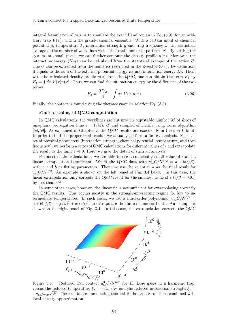
3. Tan’s contact for trapped Lieb-Liniger bosons at finite temperature
integral formulation allows us to simulate the exact Hamiltonian in Eq. (5.9), for an arbi-trary trap V (x), within the grand-canonical ensemble. With a certain input of chemicalpotential µ, temperature T , interaction strength g and trap frequency ω, the statisticalaverage of the number of worldlines yields the total number of particles N . By cutting thesystem into small pixels, we can further compute the density profile n(x). Moreover, theinteraction energy 〈Hint〉 can be calculated from the statistical average of the action U .The U can be extracted from the numerics restricted in the Z-sector 〈U〉Z . By definition,it equals to the sum of the external potential energy E1 and interaction energy E2. Then,with the calculated density profile n(x) from the QMC, one can obtain the term E1 byE1 =
∫dx V (x)n(x). Thus, we can find the interaction energy by the difference of the two
terms
E2 =〈U〉Zβ−∫dx V (x)n(x) (3.26)
Finally, the contact is found using the thermodynamics relation Eq. (3.3).
Finite-ε scaling of QMC computation
In QMC calculations, the worldlines are cut into an adjustable number M of slices ofimaginary propagation time ε = 1/MkBT and sampled efficiently using worm algorithm[58, 59]. As explained in Chapter 2, the QMC results are exact only in the ε → 0 limit.In order to find the proper final results, we actually perform a finite-ε analysis. For eachset of physical parameters (interaction strength, chemical potential, temperature, and trapfrequency), we perform a series of QMC calculations for different values of ε and extrapolatethe result to the limit ε→ 0. Here, we give the detail of such an analysis.
For most of the calculations, we are able to use a sufficiently small value of ε and alinear extrapolation is sufficient. We fit the QMC data with a3
hoC/N5/2 = a + b(ε/β),
with a and b as fitting parameters. Then, we use the quantity a as the final result fora3hoC/N
5/2. An example is shown on the left panel of Fig. 3.4 below. In this case, thelinear extrapolation only corrects the QMC result for the smallest value of ε (ε/β = 0.01)by less than 4%.
In some other cases, however, the linear fit is not sufficient for extrapolating correctlythe QMC results. This occurs mostly in the strongly-interacting regime for low to in-termediate temperatures. In such cases, we use a third-order polynomial, a3
hoC/N5/2 =
a+ b(ε/β) + c(ε/β)2 + d(ε/β)3, to extrapolate the finite-ε numerical data. An example isshown on the right panel of Fig. 3.4. In this case, the extrapolation corrects the QMC
Figure 3.3: Reduced Tan contact a3hoC/N
5/2 for 1D Bose gases in a harmonic trap,versus the reduced temperature ξT = −a1D/λT and the reduced interaction strength ξγ =−aho/a1D
√N . The results are found using thermal Bethe ansatz solutions combined with
local density approximation.
63

3. Tan’s contact for trapped Lieb-Liniger bosons at finite temperature
Figure 3.4: Quantum Monte Carlo (QMC) results for the reduced Tan contact for ξT =|a1D|/λT = 0.28 and ξγ = aho/|a1D|
√N = 0.1 (left panel) and for ξT = 0.0085 and ξγ = 4.47
(right panel). The red points show the QMC results for various values of the dimensionlessparameter ε/β, where β = 1/kBT is the inverse temperature, together with a linear (leftpanel) or third-order polynomial (right panel) fit.
result for the smallest value of ε (ε/β = 0.0005) by roughly 25%.Nevertheless, for all the QMC results reported in this thesis, we have performed a
systematic third-order polynomial extrapolation, even when a linear extrapolation wassufficient.
The validation of the scaling function
For checking the validation of the scaling as well as LDA, we check in detail the QMCdata along cuts on Fig. 3.3. In Fig. 3.5(a), we plot the contact a3
1DC as a function ofthe interaction strength ξγ for various values of the temperature via the quantity ξT =−a1D/λT = 0.0085 (blue), 0.28 (green), and 18.8 (red). For each ξT, we also try to covera broad set of parameters, which corresponds to the various symbols |a1D|/aho = 9.5 (redsquares), 0.032 (red diamonds), 1.41 (green squares), 0.14 (green diamonds), 0.14 (bluesquares), and 2.02 (blue diamonds). Here, one may notice that the scaling of the contact
Figure 3.5: Tan contact versus the scaling parameters from QMC calculations (points).The contact is rescaled in two different ways: (a). The Monte-Carlo scaling a3
1DC. (b).The scaling in the function f : a3
hoC/N5/2. The colors indicate the fixed temperatures
ξT = −a1D/λT = 0.0085 (blue), 0.28 (green), and 18.8 (red). The different symbols indicatedifferent set of parameters, namely |a1D|/aho = 9.5 (red squares), 0.032 (red diamonds),1.41 (green squares), 0.14 (green diamonds), 0.14 (blue squares), and 2.02 (blue diamonds).
64
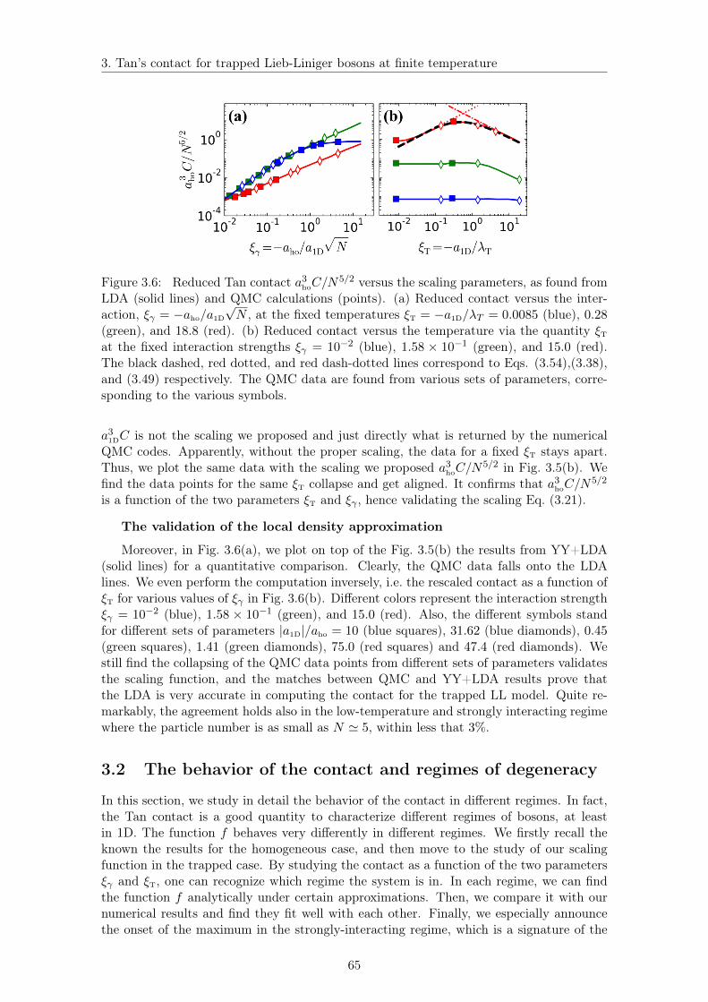
3. Tan’s contact for trapped Lieb-Liniger bosons at finite temperature
Figure 3.6: Reduced Tan contact a3hoC/N
5/2 versus the scaling parameters, as found fromLDA (solid lines) and QMC calculations (points). (a) Reduced contact versus the inter-action, ξγ = −aho/a1D
√N , at the fixed temperatures ξT = −a1D/λT = 0.0085 (blue), 0.28
(green), and 18.8 (red). (b) Reduced contact versus the temperature via the quantity ξTat the fixed interaction strengths ξγ = 10−2 (blue), 1.58 × 10⁻¹ (green), and 15.0 (red).The black dashed, red dotted, and red dash-dotted lines correspond to Eqs. (3.54),(3.38),and (3.49) respectively. The QMC data are found from various sets of parameters, corre-sponding to the various symbols.
a31DC is not the scaling we proposed and just directly what is returned by the numerical
QMC codes. Apparently, without the proper scaling, the data for a fixed ξT stays apart.Thus, we plot the same data with the scaling we proposed a3
hoC/N5/2 in Fig. 3.5(b). We
find the data points for the same ξT collapse and get aligned. It confirms that a3hoC/N
5/2
is a function of the two parameters ξT and ξγ , hence validating the scaling Eq. (3.21).
The validation of the local density approximation
Moreover, in Fig. 3.6(a), we plot on top of the Fig. 3.5(b) the results from YY+LDA(solid lines) for a quantitative comparison. Clearly, the QMC data falls onto the LDAlines. We even perform the computation inversely, i.e. the rescaled contact as a function ofξT for various values of ξγ in Fig. 3.6(b). Different colors represent the interaction strengthξγ = 10−2 (blue), 1.58 × 10⁻¹ (green), and 15.0 (red). Also, the different symbols standfor different sets of parameters |a1D|/aho = 10 (blue squares), 31.62 (blue diamonds), 0.45(green squares), 1.41 (green diamonds), 75.0 (red squares) and 47.4 (red diamonds). Westill find the collapsing of the QMC data points from different sets of parameters validatesthe scaling function, and the matches between QMC and YY+LDA results prove thatthe LDA is very accurate in computing the contact for the trapped LL model. Quite re-markably, the agreement holds also in the low-temperature and strongly interacting regimewhere the particle number is as small as N ' 5, within less that 3%.
3.2 The behavior of the contact and regimes of degeneracy
In this section, we study in detail the behavior of the contact in different regimes. In fact,the Tan contact is a good quantity to characterize different regimes of bosons, at leastin 1D. The function f behaves very differently in different regimes. We firstly recall theknown the results for the homogeneous case, and then move to the study of our scalingfunction in the trapped case. By studying the contact as a function of the two parametersξγ and ξT, one can recognize which regime the system is in. In each regime, we can findthe function f analytically under certain approximations. Then, we compare it with ournumerical results and find they fit well with each other. Finally, we especially announcethe onset of the maximum in the strongly-interacting regime, which is a signature of the
65

3. Tan’s contact for trapped Lieb-Liniger bosons at finite temperature
Figure 3.7: The local correlation g(2) versus interaction γ at different temperature τ . Thesolid curves are exact numerical results while the dashed lines are analytical formulas. Theplot is from [134].
crossover to fermionized regime.
3.2.1 The behavior of the contact in the homogeneous case
Before discussing the behavior of the contact for the 1D trapped bosons, we firstly presentthe known results of the contact in homogeneous case. In [134], the authors studiedthe two-body correlation function g(2) = 〈Ψ†Ψ†ΨΨ〉/n2 for 1D homogeneous bosons invarious regimes, with Ψ the field operator. The interaction and temperature parametersare chosen as the Lieb-Liniger parameter γ and the reduced temperature τ = T/Td withTd = ~2n2/2m the degeneracy temperature. The result is shown in Fig. 3.7.
In the case of 1D homogeneous bosons, the Tan contact C can be mapped to thequantity g(2) by the relation
g(2) =~4
m2g2n2LC. (3.27)
Therefore, the results shown in Fig. 3.7 reflects the behavior of the contact. In low tem-perature limit (see for instance τ = 0.001), the result fits well with the prediction of Som-merfield expansion of ideal fermions in the strongly-interacting regime, while it matchesthe Gross-Pitaevskii prediction in the weakly-interacting regime. In the high temperaturelimit (see for instance τ = 1000), the quantum degeneracy is broken and the behaviorfits well with what is predicted by the decoherent bosons. Here, we would like to drawthe attention of readers to an important point. According to the results in Fig. 3.7, atany regimes, for a fixed coupling constant g and particle density n, the Tan contact al-ways increases with temperature. In the next subsection, we will see that the contactbehaves non-monotonically due to the influence of the harmonic trap, where an interestingphenomenon appears.
3.2.2 The scaling function in different regimes
The regimes of degeneracies for the 1D trapped bosons have been discussed in Refs. [70,134],with another pair of parameters N and T/~ω and a fixed value −aho/a1D = 10. Here, weextend the discussion to more general cases using the two scaling parameters we mentionedabove, namely the temperature parameter ξT and the interaction parameter ξγ , see Fig. 3.8.In the following, we will explain the condition of each regime, and then give the analyticalform for the contact.
66
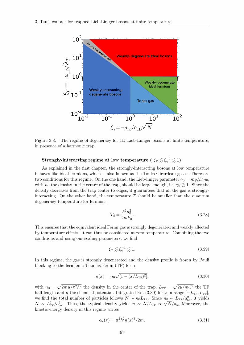
3. Tan’s contact for trapped Lieb-Liniger bosons at finite temperature
Figure 3.8: The regime of degeneracy for 1D Lieb-Liniger bosons at finite temperature,in presence of a harmonic trap.
Strongly-interacting regime at low temperature ( ξT . ξ−1γ . 1)
As explained in the first chapter, the strongly-interacting bosons at low temperaturebehaves like ideal fermions, which is also known as the Tonks-Girardeau gases. There aretwo conditions for this regime. On the one hand, the Lieb-liniger parameter γ0 = mg/~2n0,with n0 the density in the centre of the trap, should be large enough, i.e. γ0 & 1. Since thedensity decreases from the trap center to edges, it guarantees that all the gas is strongly-interacting. On the other hand, the temperature T should be smaller than the quantumdegeneracy temperature for fermions,
Td =~2n2
0
2mkB. (3.28)
This ensures that the equivalent ideal Fermi gas is strongly degenerated and weakly affectedby temperature effects. It can thus be considered at zero temperature. Combining the twoconditions and using our scaling parameters, we find
ξT . ξ−1γ . 1. (3.29)
In this regime, the gas is strongly degenerated and the density profile is frozen by Pauliblocking to the fermionic Thomas-Fermi (TF) form
n(x) = n0
√[1− (x/LTF)2], (3.30)
with n0 =√
2mµ/π2~2 the density in the center of the trap, LTF =√
2µ/mω2 the TFhalf-length and µ the chemical potential. Integrated Eq. (3.30) for x in range [−LTF, LTF],we find the total number of particles follows N ∼ n0LTF. Since n0 ∼ LTF/a
2ho, it yields
N ∼ L2TF/a
2ho. Thus, the typical density yields n ∼ N/LTF ∝
√N/aho Moreover, the
kinetic energy density in this regime writes
eK(x) = π2~2n(x)3/2m. (3.31)
67

3. Tan’s contact for trapped Lieb-Liniger bosons at finite temperature
The contact can then be found from the Bose-Fermi mapping [139]
C = (4m/~2)
∫dxn(x)eK(x). (3.32)
Inserting the Eq. (3.30) and Eq. (3.31) into the Fermi formula above and computing theintegration, we find
C =256√
2
45π2
N5/2
a3ho
, ξT . ξ−1γ . 1. (3.33)
This formula also matches the results in Ref. [121], where the authors obtain it from theBethe ansatz result of the strong interaction limit.
Strongly-interacting regime at intermediate temperature (ξ−1γ . ξT . 1)
When we are in the condition
1 .T
Td. γ2
0 , (3.34)
the temperature is larger than the Fermi degeneracy temperature. Moreover, rewritingT/Td . γ2
0 , we find a1D . λT , which indicates the 1D scattering length a1D is still smallerthan the De Broglie wavelength λT . In this regime, both quantum and thermal fluctuationsare dominated by repulsive interactions and the gas is still fermionized although with weakdegeneracy. Thus, the gases can be treated as weakly-degenerate Fermions. Rewriting thecondition of the regime Eq (3.34) with our scaling parameters, we find
ξ−1γ . ξT . 1 (3.35)
Since the gas is weakly degenerate, the kinetic energy density of the equivalent ideal Fermigas follows from the equipartition theorem of the kinetic part, i.e.
eK(x) =n(x)kBT
2(3.36)
and the density profile can be taken as the noninteracting one,
n(x) =
(N√
2πLth
)exp(−x2/2L2
th) (3.37)
with Lth =√kBT/mω2. The contact is then found from the Bose-Fermi mapping Eq. (3.32).
It yields
C =2√
2N5/2ξγξTa3ho
, ξ−1γ . ξT . 1, (3.38)
which increases as√T with temperature. It thus recovers the results of Ref. [18] by a
different approach where the regime is called non-degenerate fermions.
The weakly interacting regime at low temperature (1, ξT . ξ−1γ )
In the weakly-interacting regime, γ0 . 1, the gas is never fermionized. At low enoughtemperature, i.e. kBT . N~ω, the gas forms a quasicondensate characterized by suppresseddensity fluctuations and the density profile follows the one of Thomas-Fermi type [70,134]. 1
We can rewrite the conditions mentioned above with our scaling parameters. On the onehand, since n ∼
√N/aho (demonstration similarly as the Thomas-Fermi profile in the
strongly-interacting regime), the condition γ0 . 1 indicates ξγ . 1. On the other hand,1Within this regime, when kBT < N~2ω2/2µ, the phase fluctuation is also suppressed and the system
forms a true condensate.
68
3. Tan’s contact for trapped Lieb-Liniger bosons at finite temperature
for the condition kBT . N~ω, replacing the term N and T with proper power of ξγ andξT correspondingly, we find ξTξγ . 1. Combining the two conditions, it yields
1, ξT . ξ−1γ . (3.39)
This regime is named as "Weakly-interacting degenerate bosons" in Fig. 3.8. It is alsocalled "GP regime" in Ref. [134], since the system can be described by the Gross-Pitaevskiiequation. The contact can be found from the mean-field expression for the interactionenergy,
〈Hint〉 =1
2
∫dx gn(x)2, (3.40)
where the density profile can be described by the Thomas-Fermi (TF) density profile
n(x) =µ
g(1− x2/L2
TF) (3.41)
with LTF =√
2µ/mω2. Inserting Eq. (3.41) into Eq. (3.40), we shall obtain the interactionenergy. Thanks to the sweep relation Eq. (3.3), we then find the contact
C = ηN5/2ξ
5/3γ
a3ho
, 1, ξT . ξ−1γ (3.42)
with η = 4× 32/3/5. It’s possible to find the very weak Bogouliubov corrections on top ofit and one can show that the small temperature effect in low temperature regime leads toa very weak increase of the contact versus the temperature.
The weakly interacting regime at intermediate temperature ( ξ−1γ . ξT .
ξ−2γ )
When kBT > N~ω, the gas enters a decoherent regime. Equivalently it writes ξTξγ & 1.In this regime, the Thomas-Fermi profile is not valid any more, since the interactions arenegligible and the bosons form a nearly ideal degenerate gas [70, 134]. However, if thetemperature is smaller than the quantum degeneracy temperature, i.e. T . Td, the densityprofile remains its quantum property and writes
n(x) = λ−1T Li1/2
[exp
(α− x2
2L2th
)](3.43)
with α(ξγ , ξT) = ln[1 − exp(−1/(2πξ2γξ
2T))]. This regime is referred as "Degenerate ideal
bosons" in Fig. 3.8. Here, one should notice that although the parameter Td is intro-duced by Eq. (3.28) as the degeneracy temperature for the fermionized bosons in strongly-interaction regime, it also characterizes the competition between the inter-particle separa-tion and the de Broglie wavelength. Taking into consideration n ∼ N/Lth, the conditionfor the weakly-interacting degenerate Bose regime can be rewritten with the scaling pa-rameters as
ξ−1γ . ξT . ξ−2
γ (3.44)
Insert the profile of this regime into the interaction energy Eq. (3.40) and calculate thecontact with the sweep relation Eq. (3.3), we shall find
C =16√πN5/2ξ5
γξ3T
a3ho
G(α), ξ−1γ . ξT . ξ−2
γ (3.45)
with G(α) the integration of the polylogarithm function, which writes
G(α) =
∫dx Li21/2[exp(α− x2)]. (3.46)
69

3. Tan’s contact for trapped Lieb-Liniger bosons at finite temperature
Figure 3.9: The function G(Γ) with Γ = ξ2Tξ
2γ (solid black line). The dashed blue line is
H(Γ) = 0.03Γ3/2 ∼ ξ3T which indicates that G(Γ) decreases faster than ξ3
T.
Studying the temperature dependence of the function G(α), we define Γ = ξ2Tξ
2γ and
plot the function G(Γ), see solid black line in Fig. 3.9. In comparision, we also plotH(Γ) = 0.03Γ3/2 which is proportional to ξ3
T, see blue dashed line. In the log-log scale, itis clear that G(α) decreases faster than ξ3
T in the regime ξTξγ ∼ 1. Using Eq. (3.45), itindicates that the contact C decreases with the temperature T . Here, we recall C increaseswith T in the low temperature regime, hence it indicates that there is a maximum of thecontact even in the weakly-interacting regime. We will study the property of this maximumin the next section.
High temperature classical regime (ξ−1γ , 1 .
√ξT)
For both the strongly- or weakly-interacting gases, the high temperature regime presentsthe same property and its condition yields the temperature is higher than any relevanttemperature scale: T > Td and a1D > λT . Rewriting this two conditions in our scalingparameters (demonstration similar as before), we find
1, γ20 .
T
Td. (3.47)
Rewritting it with our scaling parameters, we find
ξ−1γ , 1 .
√ξT. (3.48)
In this regime, one obtains a weakly degenerate Bose gas dominated by thermal fluctua-tions. We refer it as "Weakly-degenerate ideal bosons" in Fig. 3.8. In this case, the contactcan still be estimated by the mean-field expression of the interaction energy Eq. (3.40).However, the density profile loses its quantum property and behaves like the thermalBoltzman distribution Eq. (3.37). Combining these two equations with the sweep relationEq. (3.3), we find
C ' 2√
2N5/2ξγπξTa3
ho
, ξ−1γ , 1 .
√ξT. (3.49)
Here, at any interaction but high temperature, we may notice that the contact decreaseswith temperature as 1/
√T . And it recovers what is expected from high temperature
strongly-interacting bosons in Ref. [18].
70

3. Tan’s contact for trapped Lieb-Liniger bosons at finite temperature
Figure 3.10: Behavior of the temperature at which the contact is maximum versus theinteraction strength. Shown is the value of ξ∗T (solid black line with shaded gray error bars)as found from the data of Fig. 3.3, together with the asymptotic behaviors ξ∗T ' 0.49 forthe strongly interacting regime (dashed red line) and ξ∗T ∝ ξνfitT , with νfit ' 0.6 for theweakly interacting regime (dotted blue line).
3.2.3 The onset of maximum
As we already announced in the previous section, the particularly interesting outcome hereis the nonmonotonicity of C versus temperature and the onset of a maximum, for examplesee Fig. 3.6(b). In fact, this behavior strongly contrasts with the previous results found forthe homogeneous gas and the trapped gas in the Tonks-Girardeau limit (a1D → 0), whichare both characterized by a systematic increase of the contact versus temperature [18,134].In the trapped case, the maximum in the contact as a function of ξT is found irrespective tothe strength of interactions but is significantly more pronounced in the strongly interactingregime. From the data of Fig. 3.3, we extract the temperature T ∗ at which the contact ismaximum at fixed ξγ . In Fig. 3.10, we plot the corresponding ξ∗T = −a1D/λ∗T as a functionof ξγ . As we can see, ξ∗T shows significantly different behavior in the strongly and weaklyinteracting regimes. It depends on the value of ξγ in the weakly-interacting regime andremain constant in strongly-interacting regime. Now, we study in detail the origin of themaximum and its physical meaning.
Maximum in the strong interaction regime
In strongly-interacting regime, ρ(0)|a1D| . 1, we stress that both Eqs. (3.38) and (3.49)are in good agreement with the numerical calculations, see red-dotted and dash-dotted linesin Fig. 3.6(b). These expressions show that the contact increases with temperature in thefermionized regime but decreases when thermal fluctuations dominate over interactions,which is the origin of the existence of maximum. It provides a nonambiguous signature ofthe crossover to fermionization and we will analysis this into detail now.
We can obtain the analytical expression for the contact using the virial expansion.Here, I would like to point out that the whole derivation in this part has been done byProf. Patrizia Vignolo. To start with, we recall the expression of the grand potential instatistical physics,
Ω = −kBT lnZ (3.50)
with Z the partition function. By performing the virial expantion to the grand potentialas in Ref. [18, 140], it writes
Ω = −kBTQ1(z + b2z2 + b3z
3 + ...) (3.51)
71

3. Tan’s contact for trapped Lieb-Liniger bosons at finite temperature
with z = eβµ the fugacity and bn the n-th virial expansion coefficient related with Qn =Trn[exp(−H/kBT )]. The bn can be calculated from the cluster partition functions [141],for instance, b2 = Q2/Q1−Q1/2. Using the Tan sweep relation Eq. (3.2) and keeping onlythe z2 term, one can find
C =4mω
~λTN2 c2 (3.52)
where c2 = λT∂b2∂|a1D|
and b2 =∑
ν e−β~ω(ν+1/2). The ν’s are the solutions of the transcen-
dental equation [142]
f(ν) =Γ(−ν/2)
Γ(−ν/2 + 1/2)=√
2a1Daho
. (3.53)
Then, with further mathematical derivation, one can solve the solution for ν in Eq. (6.2)and infer the term c2 in Eq. (6.1). The detail of this derivation is shown in the Appendix.With the solution of c2, one can find the analytical form for the contact by Eq. (6.1), ityields
C =2N5/2
πa3ho
ξγξT
(√
2− e1/2πξ2T
ξTErfc(1/
√2πξT)
), (3.54)
see black dashed line in Fig. 3.6(b). Solving ∂C/∂T = 0 in Eq. 3.54, we can locate amaximum at ξ∗T = 0.485, which is in very good agreement with the asymptotic scalingξ∗T ' 0.490± 0.005 extracted from the data (dashed red line in Fig. 3.10).
From Eq. (3.3), we can infer that the maximum of the contact is equivalent to themaximum of the interaction energy, while fixing g. Then, the existence of the maximumcan actually be understood by the competition of two processes. On the one hand, at lowtemperature, the bosons can never overlap since they are blocked by the strong repulsiveinteraction, which is equivalent to Pauli blocking in the equivalent ideal Fermi gas. Withthe increase of temperature, the bosons gain enough energy repulsion to overcome theblockade and allow a spatial overlap, thus increasing the interaction energy locally, i.e.increase the contact C. On the other hand, since the system is a many-body systemconfined in a harmonic trap, increasing the temperature will enlarge the size of the systemand dilute the gas. Therefore, the interaction energy will be reduced globally, i.e. thecontact C will decrease. As a consequence, the competing of these two processes leads tothe non-monotonic temperature effect of the contact. It forms a maximum when the effectof both are on the same scale. In another word, due to the competition of interaction andtemperature, the maximum contact should appear at the temperature where the interactionand dilution effect reaches the same magnitude. According to Fig. 3.8, this crossoverhappens at ξT ∼ 1 when ξγ > 1, i.e. in length scale a1D ∼ λT , which fit well with what wefind in the previous calculations.
We further argue that the existence of this maximum is extremely interesting, sinceit is a direct consequence of the dramatic change of correlations and thus provides anunequivocal signature of the crossover to fermionization in the trapped 1D Bose gas. Forother detected quantities such as the density profile, they normally show a smooth variationwhile going through the crossover. However, the maximum of the contact provides theprobability to probe it accurately with sharp change of behavior.
Maximum in the weak interaction regime
The maximum in the weak interaction regime is much weaker, but it is still possible forus to capture it from the theoretical point of view. For low temperature regimes, the contactfollows Eq. (3.42) with Bogoliubov correction term increasing with T . Then, for highertemperature, the contact follows Eq. (3.45) where C decreases with the temperature thanksto the property of G as we discussed above. Since the contact increases with temperature
72

3. Tan’s contact for trapped Lieb-Liniger bosons at finite temperature
at low T , due to the weak Bogoliubov excitations, we can conclude that there also existsthe maximum contact in the weakly-interacting regime and it signals the crossover fromthe quasicondensate regime to the ideal Bose gas regime. The position of the maximumof the contact may be estimated by equating Eqs. (3.42) and (3.45). The calculation issignificantly simplified by neglecting quantum degeneracy effects and treat the densityprofile as a Gaussian in Eq. (3.45). Then, it yields
G(α) '√π/2 exp(2α) (3.55)
Performing the Taylor expansion for G(α) as a function of Γ = ξ2Tξ
2γ , we find G(α) ' Γ−2 ∼
1/ξ4γξ
4T and we have checked by numerical plotting that this approximation is valid up to
the regime ξγξT ∼ 1. Then, equating Eqs. (3.42) and (3.45) with the function G(α) above,we finally find
ξ∗T ∼ ξ−νγ , ν = 2/3. (3.56)
To check this prediction, we have fitted by Eq. (3.56) with ν as an adjustable parameter(see dotted blue line in Fig. 3.10), yielding νfit = 0.6 ± 0.06, in good agreement with thetheoretical estimate νth = 2/3. However, quantum degeneracy effects tend to increase thevalue of ν for small values of ξγ . In the asymptotic limit ξγ → 0, they become dominant.In this limit, we find G(α) ' π2/
√|α| and it yields ν ' 1. Nevertheless, we should point
out that the maximum is extremely weak and hardly visible in practice in this regime.
The maximum of entropy
To further interpret the onset of a maximum contact versus temperature, we realise thatit is actually equivalent to the onset of a maximum entropy S versus interaction strength.For a fixed number of particles, it is a direct consequence of the Maxwell identity. Here,we recall the definition of the free energy F in thermodynamics
F (N,T, a1D) = Ω(µ, T, a1D) + µN, (3.57)
where we change the variables from µ to N . Then, we can rewrite the sweep relation forthe contact in term of the free energy and it gives
C =4m
~2
∂F
∂a1D
∣∣∣∣T,N
. (3.58)
Moreover, we use the thermodynamic definition of the entropy
S = − ∂F
∂T
∣∣∣∣a1D,N
. (3.59)
Combining Eq. (3.58) and Eq.( 3.59), we find
∂C
∂T
∣∣∣∣a1D,N
= −4m
~2
∂S
∂a1D
∣∣∣∣T,N
, (3.60)
which indicates that the two maximums appear at the same set of parameters. In thehomogeneous LL gas, the entropy at fixed temperature and number of particles decreasesmonotonically versus the interaction strength, since repulsive interactions inhibit the over-lap between the particle wavefunctions. Hence, the supression of free space for particlesdiminishes the number of available configurations. In the trapped gas, however, this ef-fect competes with the interaction dependence of the available volume. More precisely,starting from the noninteracting regime, the system size increases sharply with interactionstrength, while the particle overlap varies smoothly. Therefore, in this regime, the numberof available configurations and the entropy increase with the interaction strength. At the
73

3. Tan’s contact for trapped Lieb-Liniger bosons at finite temperature
onset of fermionization, interaction-induced spatial exclusion becomes dramatic and theparticles strongly avoid each other. In turn, as opposed to the weakly-interacting regime,the volume increases very slightly. In this regime, the number of available configurationsthus decreases when the interactions increase. This picture confirms that the maximumof the entropy as a function of the interaction strength, consistently with the maximumof the contact as a function of the temperature. Thus, it also signals the fermionizationcrossover.
3.3 Experimental observability
In this section, we discuss the experimental observability of the contact and its proper-ties, especially the maximum contact in strongly-interaction regimes which signatures thecrossover to fermionization. We mainly focus on three aspects, namely the detection ac-curacy, the validity of the purely 1D gas model, and the consequence of averaging over 1Dgases with different number of particles, as relevant in experiments creating a 2D array of1D tubes.
3.3.1 Accuracy of detection
As we discussed at the beginning of this chapter, our predictions can be investigatedwith quantum gases where the Tan contact is extracted from radio-frequency spectra ormomentum distributions [125–127, 130]. To understand better the observation conditionin the later case, we compute the momentum distribution. Here, one should notice thatthe momentum distribution cannot be found from Y-Y thermodynamics. In turn, QMCcalculation can do it efficiently, see Section 2.3.4.
Figure 3.11 shows momentum distributions found from QMC calculations in the stronglyinteracting regime for two typical temperatures. Figure. 3.11(a) is close to zero tempera-ture (ξT 1) and Fig. 3.11(b) is at the temperature for the maximum contact ξT ' ξ∗T.In both cases, an algebraic decay at large momenta is observed, with an amplitude match-ing our estimate for the contact. Here, one should note the log-log scale in the mainpanels and the lin-lin scale are plotted as insets. Fitting the tails of the momentum dis-tributions found from the QMC calculations by n(k) ' Cfit/k
pfit , where we obtain pfit andCfit = a3
hoCfit/N5/2. For Fig. 3.11(a), we find pfit = 3.80±0.20 and Cfit = (1.01±0.14)×10−3
while C ' 0.97× 10⁻³. For Fig. 3.11(b), we find pfit = 3.72± 0.10 and Cfit = 0.23± 0.04while C ' 0.22. The agreement with the expected exponent p = 4 is better than 7% andwith the contact C better than 5%. Here, we notice that for the two examples shownhere, the momentum distributions decay over three to four decades. Such a range is quiteunusual. Helium atoms can however measure momentum distribution in such a rangetaking advantage of single-particle resolution. For instance, measurement of momentumdistributions in Ref. [125] covers up to six decades.
3.3.2 Validity condition of the quasi-1D regime
Focusing on the observability of the maximum, one should also be careful with the conditionto have really one-dimensional tube instead of 3D (also named as quasi-1D). In ultracoldatoms, the tubes are induced either by a magnetic field or a transverse optical lattice. Inthe second case, the system consists of arrays of 1D tubes, see Fig. 1.1. In both cases, itcreates a local transverse harmonic trap with frequency ω⊥. The condition for the suchkinds of systems to be in strictly-1D regime writes kBT, µ ~ω⊥. The condition simplymeans that the system remains in ground state for the freedom of the transverse harmonicoscillation and no significant excitation is created, see details in for instance Ref. [62].
74
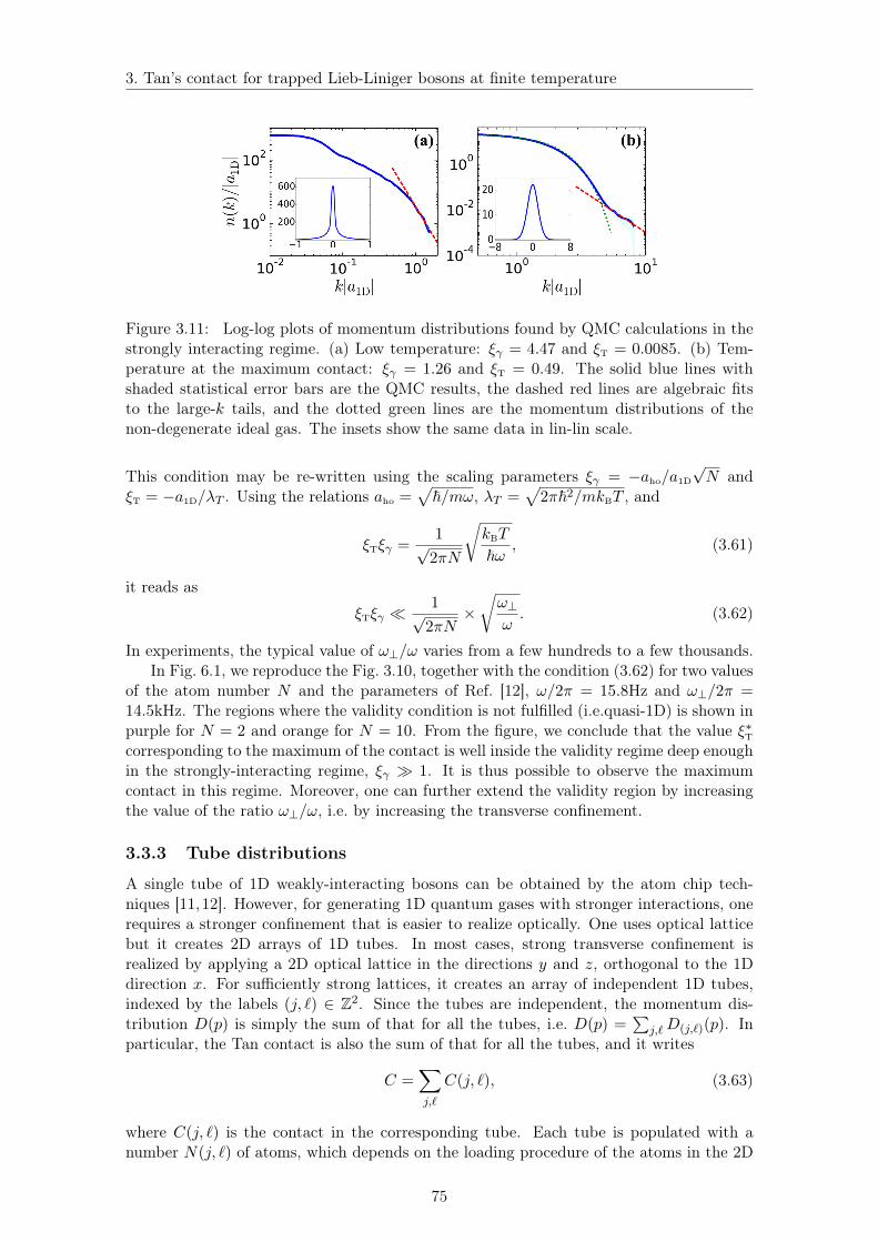
3. Tan’s contact for trapped Lieb-Liniger bosons at finite temperature
Figure 3.11: Log-log plots of momentum distributions found by QMC calculations in thestrongly interacting regime. (a) Low temperature: ξγ = 4.47 and ξT = 0.0085. (b) Tem-perature at the maximum contact: ξγ = 1.26 and ξT = 0.49. The solid blue lines withshaded statistical error bars are the QMC results, the dashed red lines are algebraic fitsto the large-k tails, and the dotted green lines are the momentum distributions of thenon-degenerate ideal gas. The insets show the same data in lin-lin scale.
This condition may be re-written using the scaling parameters ξγ = −aho/a1D√N and
ξT = −a1D/λT . Using the relations aho =√
~/mω, λT =√
2π~2/mkBT , and
ξTξγ =1√
2πN
√kBT
~ω, (3.61)
it reads as
ξTξγ 1√
2πN×√ω⊥ω. (3.62)
In experiments, the typical value of ω⊥/ω varies from a few hundreds to a few thousands.In Fig. 6.1, we reproduce the Fig. 3.10, together with the condition (3.62) for two values
of the atom number N and the parameters of Ref. [12], ω/2π = 15.8Hz and ω⊥/2π =14.5kHz. The regions where the validity condition is not fulfilled (i.e.quasi-1D) is shown inpurple for N = 2 and orange for N = 10. From the figure, we conclude that the value ξ∗Tcorresponding to the maximum of the contact is well inside the validity regime deep enoughin the strongly-interacting regime, ξγ 1. It is thus possible to observe the maximumcontact in this regime. Moreover, one can further extend the validity region by increasingthe value of the ratio ω⊥/ω, i.e. by increasing the transverse confinement.
3.3.3 Tube distributions
A single tube of 1D weakly-interacting bosons can be obtained by the atom chip tech-niques [11,12]. However, for generating 1D quantum gases with stronger interactions, onerequires a stronger confinement that is easier to realize optically. One uses optical latticebut it creates 2D arrays of 1D tubes. In most cases, strong transverse confinement isrealized by applying a 2D optical lattice in the directions y and z, orthogonal to the 1Ddirection x. For sufficiently strong lattices, it creates an array of independent 1D tubes,indexed by the labels (j, `) ∈ Z2. Since the tubes are independent, the momentum dis-tribution D(p) is simply the sum of that for all the tubes, i.e. D(p) =
∑j,`D(j,`)(p). In
particular, the Tan contact is also the sum of that for all the tubes, and it writes
C =∑j,`
C(j, `), (3.63)
where C(j, `) is the contact in the corresponding tube. Each tube is populated with anumber N(j, `) of atoms, which depends on the loading procedure of the atoms in the 2D
75

3. Tan’s contact for trapped Lieb-Liniger bosons at finite temperature
Figure 3.12: Reproduction of Fig. 3.10 together with the validity condition of the quasi-1Dregime (equivalently the regime for the failure of purely-1D gas), Eq. (3.62), for
√ω⊥/ω =
30, relevant for the experiments of Ref. [12]. The dark regions show the excluded regionsfor N = 2 atoms (purple) and N = 10 atoms (orange).
lattice. Since the number of atoms is maximum in the central tube (j = ` = 0), we haveξγ(j, `) ≥ ξγ(0, 0), and the condition for having all tubes in the strongly-interacting regimereduces to ξγ(0, 0) 1.
In that regime, the temperature dependence of the contact around the maximum isindependent of ξγ , and thus independent of the tube. Indeed, as shown by Eq. (3.54), theparameter ξγ just appears as a prefactor. In particular, the maximum contact is locatedat the universal value ξ∗T ' 0.485, which is identical for the tubes. Using Eq. (3.54), wethen find
C∗ ' 0.55×∑j,`
N(j, `)5/2ξγ(j, `)
a3ho
. (3.64)
At zero temperature, the contact may be found using the mapping between the strongly-interacting Bose gas and the strongly-degenerate ideal Fermi gas. It yields the value of thecontact at zero temperature [121]
C0 ' 0.82×∑j,`
N(j, `)5/2
a3ho
. (3.65)
We then find that the relative amplitude of the maximum contact with respect to itszero-temperature value fulfils the inequality
C∗
C0& 0.68× ξγ(0, 0). (3.66)
Therefore, the relative amplitude of the maximum contact is larger than a fraction ofthe interaction parameter ξγ(0, 0) 1 and should be observable. For instance, for theparameters of Ref. [12], we find ξγ(0, 0) ' 7.5 and C∗/C0 & 5.1.
Note that the lower bound in Eq. (3.66) is universal in the sense that it does not dependon the distribution of atoms in the various lattice tubes. Note also that it is immune toshot-to-shot fluctuations of the atom numbers in the tubes.
Finally, a more precise value of the relative amplitude of the maximum contact isfound by computing the sums in Eqs. (3.64) and (3.65) for realistic distributions of theatom numbers among the tubes. Here, using the estimation that the initial 3D BEC followsthe Thomas-Fermi profile and the loading process is fast, we shall write
Nj,` =
[1− 2πN(0, 0)
5N
(j2 + `2
)]3/2
, (3.67)
76
3. Tan’s contact for trapped Lieb-Liniger bosons at finite temperature
which is relevant to the experiments of Refs. [9, 12]. With Eq. (3.67), we find C∗/C0 '0.8 × ξγ(0, 0), which is only about 20% larger than the atom distribution-independentlower bound, Eq. (3.66). For the parameters of Ref. [12], it yields C∗/C0 & 6.1. It may befurther increased by lowering the total number of atoms, although at the expense of atomdetectability.
Conclusion
In this chapter, we have provided a complete characterization of the Tan contact forthe trapped Lieb-Liniger gas with arbitrary interaction strength, number of particles, tem-perature, and trap frequency. We first derived a universal scaling function of only twoparameters, which stand for the temperature and interaction strengths. We have shownthat it is in excellent agreement with the numerically exact QMC results as well as theYang-Yang calculations over a wide range of parameters. In different regimes of degener-acy, we found that the results of the contact fit well with the asymptotic formula as weexpected. As a pivotal result, we found that the contact exhibits a maximum versus thetemperature for any interaction strength. This behavior is mostly marked in the gas withlarge interactions and provides an unequivocal signature of the crossover to fermionization.Finally, we also analyzed the experimental observation condition for the contact, especiallythe maximum.
In the outlook, our theoretical results provides fruitful physics to be detected in experi-ments. On the one hand, its behavior as a function of the temperature and interaction canidentify regimes of degeneracy and critical behaviors. It also provides plenty of informationsuch as the interaction energy, correlation function, as well as the behaviors of the ther-modynamic quantities. On the other hand, 1D ultracold atoms created by optical latticesis a good candidate for such a detection, since it can observe the momentum distributionwith a good accuracy over 6 orders of magnitudes decaying [125], as well as entering thestrong interacting regimes with ξγ & 10 [12].
77

Chapter 4
Critical behavior in shallow 1Dquasiperiodic potentials: localizationand fractality
Anderson localization, known as the absence of diffusion of waves in a disordered medium,is one of the hottest topic of research since 20-th centry, in the framework of both condensedmatter and quantum simulations. In a homogeneous system, all the single-particle wavefunctions are extended. In contrast, they may be exponentially localized in the presenceof disorder owing to the breaking of translational invariance [143]. The effect of the phasetransition between the extended and localized state is known as the Anderson localization.It is a single-particle effect caused by disorder as well as a fundamental and ubiquitousphenomenon at the origin of metal-insulator transitions in many systems [144].
The Anderson localization and its phase transition have been widely studied in thepurely disordered systems, both the single-particle case [143,145–148] and the interactingmany-body systems [46–51, 149]. The influence of disorder in fermionic systems are alsostudied [150–153]. The quasiperiodic models, known as the intermediate between the pe-riodic and fully disordered systems, hold a special place. An illustration for the three kindsof system is shown in Fig. 4.1. While a single trigonometric function stands for the purelyperiodic system, the disordered system is the opposite case where its Fourier componentscontain infinite and dense values of different frequencies. The quasiperiodic system is theintermediate of the two, which can be understood by a sum of two or trigonometric func-tion which frequencies has an incommensurate ratio between each other and form a finiteor discrete set, i.e. no true periodicity exists. In recent years, it attracts a lot of attentionsand interests of research.
"Quasiperiodic model" describes a variety of systems. On the condensed matter side,it includes quasicrystals [154], electronic materials in orthogonal magnetic fields [155–157] or with incommensurate charge-density waves [158], Fibonacci heterostructures [159],photonic crystals [160], and cavity polaritons [161]. Moreover, on the research field ofcold atoms, it can be achieved by realizing external quasiperiodic potentials on top ofthe cold atomic gases. This kind of systems have proved pivotal in quantum gases [153,162, 163] to investigate Anderson localization of matter waves [8, 164, 165] and interactingBose gases [41], the emergence of long-range quasiperiodic order [19, 166, 167], Bose-glassphysics [14,20,21,164,165,168], and many-body localization [16,169–171].
In a disordered system, a phase transition between the Anderson-localized and extendedphases occurs only in dimension strictly higher than 2 [172]. However, in quasiperiodicsystems, the behavior is significantly different and a phase transition may occur. The mostcelebrated example is the Aubry-André (AA) Hamiltonian, obtained from the tight-bindingmodel generated by a strong lattice, combined with a second, weak, incommensurate lattice
78

4. Critical Behavior in Shallow 1D Quasiperiodic Potentials: Localization and Fractality
Figure 4.1: The typical shape for three kinds of potential: (a). Periodic. (b). Disordered.(c). Quasiperiodic, which may be a sum of several periodic potentials with incommensurateratio of lattice spacings.
serving as the quasi-disorder. In the AA model, the localization transition occurs at acritical value of the quasiperiodic potential, irrespective of the particle energy [173]. Thisbehavior results from a special symmetry, known as self-duality. When the latter is broken,an energy mobility edge (ME), i.e. a critical energy separating localized and extendedstates, generally appears, as demonstrated in a variety of models [31, 174–179]. One ofthe simplest examples is obtained by using two incommensurate lattices of comparableamplitudes, which refers to a shallow or continuous bichromatic lattice. This model attractssignificant attention in ultracold-atom systems owing to the fact that it is generally easierto realize compared to truly disordered systems [180, 181]. They have been used to studymany-body localization in a 1D system exhibiting a single-particle ME [16]. Recently, thelocalization properties and the ME of the single-particle problem have been studied boththeoretically [181] and experimentally [182]. However, important critical properties of thismodel are still unknown. For instance, whether an intermediate phase appears in betweenthe localized and extended phases remains unclear.
In this chapter, we study the critical properties and the fractality of noninteractingparticles in shallow quasiperiodic potentials [86]. We firstly introduce the important con-cepts in this problem, such as the definition of a localized state, the critical potential andthe mobility edge(ME). Then, we start the study with balanced bichromatic lattices. Withbalanced amplitude, we find that a finite energy ME exist above a certain critical ampli-tude of potential Vc. We determine its value from the scaling of the inverse participationratio and find the universal critical exponent ν ' 1/3. We further extend the investigationto more generalized case, i.e. bichromatic lattices with imbalanced amplitudes as well astrichromatic lattices, and we find the results remain the same. Finally, we find the ME isalways found in one of the energy gaps, which are dense thanks to the fractal character ofthe energy spetrum. We propose a method to compute the critical Hausdorff dimensionand find values significantly different from that found for the AA model, showing that it isa non-universal quantity. In all the considered cases, we remain the lattice amplitudes onthe scale of the recoil energy Er = ~2k2/2m, to maintain in the shallow potential regime.
79

4. Critical Behavior in Shallow 1D Quasiperiodic Potentials: Localization and Fractality
4.1 Localization, disorder and quasiperiodicity
In this section, we introduce the basic concepts and standard models used in this chapter.We first demonstrate several important definitions in this chapter, such as the extendedand localized states, the mobility edge(ME) and the critical potential (Vc). Then, we gothrough some well-known examples and discuss in detail the localization property.
4.1.1 Basic concepts for localization
Before we move on to present the scientific results, it’s important to give the rigorousdefinition of several key quantities at this stage.
Extended and localized phases
The difference between the extended and localized phases is illustrated on Fig. 4.2. Inthe diagram, the black curve stands for the external potential and the blue wave packetsstand for the eigenstate wavefunction. We use L for the size of the system and l the typicalwidth of the certain eigenstate. From the left panel to the right panel, we double the sizeof the system and keep all the other parameters unchanged. On the upper row, the systemis in the localized phase so that the width of the eigenstate remains constant. On the lowerrow, the width of the eigenstate also doubles similarly as the size of the system, thus it isdefined as extended state.
Figure 4.2: Illustration of the difference between localized and extended states. The blackcurve stands for the external potential and the blue wave package stand for the eigenstate.L is the size of the system and l is the width of the eigenstate.
The localization property of an eigenstate ψ can be characterized by the second-orderinverse participation ratio (IPR) [183],
IPR =
∫dx |ψn(x)|4(∫dx |ψn(x)|2
)2 . (4.1)
with ψn(x) the wavefunction of the n-th eigenstate. If the state ψn(x) is a wavepacket withtypical size l, then we have IPR ∼ 1/l and the value of itself thus gives an estimation ofthe localization. However, we have to be careful that it is rather a measure of the fractionof space that it covered by the space. Thus, there exists cases where the value of IPR doesnot say much about the localization. For instance, for a deep periodic lattices, the localcompression at the bottom of the wells leads to IPR 1 although the state is extended.
80
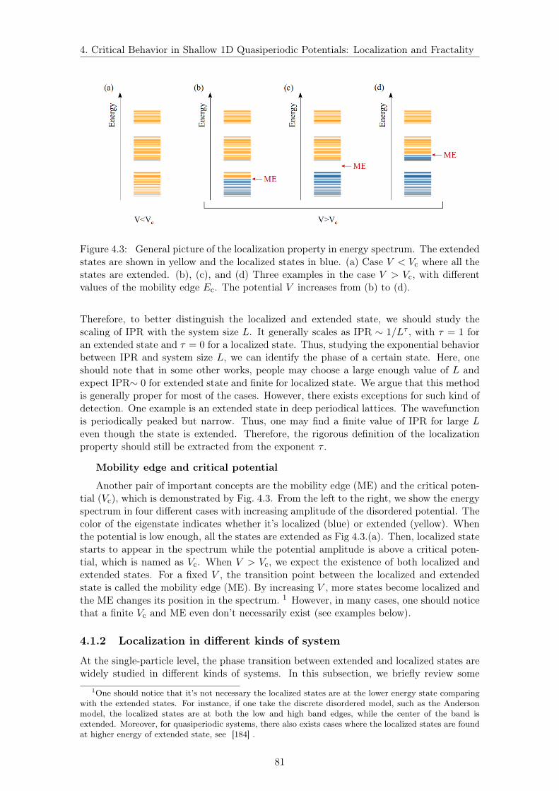
4. Critical Behavior in Shallow 1D Quasiperiodic Potentials: Localization and Fractality
Figure 4.3: General picture of the localization property in energy spectrum. The extendedstates are shown in yellow and the localized states in blue. (a) Case V < Vc where all thestates are extended. (b), (c), and (d) Three examples in the case V > Vc, with differentvalues of the mobility edge Ec. The potential V increases from (b) to (d).
Therefore, to better distinguish the localized and extended state, we should study thescaling of IPR with the system size L. It generally scales as IPR ∼ 1/Lτ , with τ = 1 foran extended state and τ = 0 for a localized state. Thus, studying the exponential behaviorbetween IPR and system size L, we can identify the phase of a certain state. Here, oneshould note that in some other works, people may choose a large enough value of L andexpect IPR∼ 0 for extended state and finite for localized state. We argue that this methodis generally proper for most of the cases. However, there exists exceptions for such kind ofdetection. One example is an extended state in deep periodical lattices. The wavefunctionis periodically peaked but narrow. Thus, one may find a finite value of IPR for large Leven though the state is extended. Therefore, the rigorous definition of the localizationproperty should still be extracted from the exponent τ .
Mobility edge and critical potential
Another pair of important concepts are the mobility edge (ME) and the critical poten-tial (Vc), which is demonstrated by Fig. 4.3. From the left to the right, we show the energyspectrum in four different cases with increasing amplitude of the disordered potential. Thecolor of the eigenstate indicates whether it’s localized (blue) or extended (yellow). Whenthe potential is low enough, all the states are extended as Fig 4.3.(a). Then, localized statestarts to appear in the spectrum while the potential amplitude is above a critical poten-tial, which is named as Vc. When V > Vc, we expect the existence of both localized andextended states. For a fixed V , the transition point between the localized and extendedstate is called the mobility edge (ME). By increasing V , more states become localized andthe ME changes its position in the spectrum. 1 However, in many cases, one should noticethat a finite Vc and ME even don’t necessarily exist (see examples below).
4.1.2 Localization in different kinds of system
At the single-particle level, the phase transition between extended and localized states arewidely studied in different kinds of systems. In this subsection, we briefly review some
1One should notice that it’s not necessary the localized states are at the lower energy state comparingwith the extended states. For instance, if one take the discrete disordered model, such as the Andersonmodel, the localized states are at both the low and high band edges, while the center of the band isextended. Moreover, for quasiperiodic systems, there also exists cases where the localized states are foundat higher energy of extended state, see [184] .
81
4. Critical Behavior in Shallow 1D Quasiperiodic Potentials: Localization and Fractality
results in one dimension.
Periodic and disordered system
The 1D periodic system is a standard model for electronic systems, see for instancethe Bloch theorem. The ultracold atomic system is a clean realization where the externalpotential is exactly trigonometric function V (x) = V cos (2kx) with V the potential ampli-tude and k the wave vector. The lattice spacing a = π/k gives the spatial period. In suchkind of systems, it is well known that all single particle states are extended no matter howlarge the amplitude of the potential. Thus, there is no critical potential and ME in such asystem.
The situation is opposite in the purely disordered system. In this case, there is no phasetransition in one dimension and all the eigenstates are localized as soon as the potential isnon-zero. Thus, there is no Vc and ME in this situation. A phase transition between theAnderson-localized and extended phases can only occur in dimension strictly higher than2 [172]. Therefore, as an intermediate situation between periodic and disordered one, wemay expect that in a one-dimensional quasiperiodic system, we can obtain a finite Vc anda finite ME.
Aubry-André model
The typical form of the bichromatic quasiperiodic lattices writes
V (x) =V1
2cos (2k1x) +
V2
2cos (2k2x+ ϕ) , (4.2)
where the quantities Vj (j = 1, 2) are the amplitudes of two periodic potentials of incom-mensurate spatial periods π/kj with k2/k1 = r, an irrational number. The Aubry-André(AA) model is one of the most widely studied bichromatic quasiperiodic model in 1D since1950s [173]. The external potential takes the tight-binding limit of Eq. (4.2) generated bya strong lattice. The second is weak and has an incommensurate lattice spacing with thefirst lattice r = (
√5− 1)/2. Equivalently, it yields the condition
V1 V2, Er, E′r (4.3)
with Er = ~2k21/2m and E′r = ~2k2
2/2m the recoil energy of the first and second lattice.Since V1 is much larger than any recoil energy, the system can be treated discretized asthe tight-binding model. Moreover, since V2 is much smaller than the band gap of thefirst lattices, the second lattice can serve as a perturbation of the first lattice and one canrestrict to the first band of the first lattice. Then, the single-particle Hamiltonian can bewritten as
HAA = −J∑〈i,j〉
(a†i aj + H.c.
)+ ∆
∑i
cos(2πri+ ϕ)a†i ai, (4.4)
where ai is the annihilation operator of a particle in the lattice site i (located at the positionxi = a × i), J is the tunneling energy associated to lattice 1 and ∆ is the quasi-periodicamplitude induced by lattice 2. The AA parameters J and ∆ in Eq. (4.4) can be relatedto the parameters of the two lattices V1 and V2 by
J ' 4Er√π
(V1
Er
)3/4
exp
(−2
√V1
Er
)with ∆ ' V2
2exp
(−r2
√Er
V1
). (4.5)
The detailed derivation can be found in Refs. [164,177].In the AA model, it is well known that the phase transition happens at the critical
potential ∆c/2J = 1. However, there is no ME existed. For ∆/2J > 1, all states arelocalized while for ∆/2J < 1 all states are extended. In the next section, we focus thelocalization phase transition of shallow quasiperiodic lattice, i.e.V1 ∼ V2 ∼ Er and studythe critical behaviors.
82
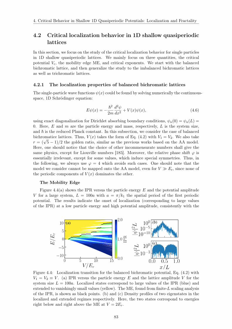
4. Critical Behavior in Shallow 1D Quasiperiodic Potentials: Localization and Fractality
4.2 Critical localization behavior in 1D shallow quasiperiodiclattices
In this section, we focus on the study of the critical localization behavior for single particlesin 1D shallow quasiperiodic lattices. We mainly focus on three quantities, the criticalpotential Vc, the mobility edge ME, and critical exponents. We start with the balancedbichromatic lattice, and then generalize the study to the imbalanced bichromatic latticesas well as trichromatic lattices.
4.2.1 The localization properties of balanced bichromatic lattices
The single-particle wave functions ψ(x) could be found by solving numerically the continuous-space, 1D Schrödinger equation:
Eψ(x) = − ~2
2m
d2ψ
dx2+ V (x)ψ(x), (4.6)
using exact diagonalization for Dirichlet absorbing boundary conditions, ψn(0) = ψn(L) =0. Here, E and m are the particle energy and mass, respectively, L is the system size,and ~ is the reduced Planck constant. In this subsection, we consider the case of balancedbichromatice lattices. Thus, V (x) takes the form of Eq. (4.2) with V1 = V2. We also taker = (
√5 − 1)/2 the golden ratio, similar as the previous works based on the AA model.
Here, one should notice that the choice of other incommensurate numbers shall give thesame physics, except for Liouville numbers [185]. Moreover, the relative phase shift ϕ isessentially irrelevant, except for some values, which induce special symmetries. Thus, inthe following, we always use ϕ = 4 which avoids such cases. One should note that themodel we consider cannot be mapped onto the AA model, even for V Er, since none ofthe periodic components of V (x) dominates the other.
The Mobility Edge
Figure 4.4(a) shows the IPR versus the particle energy E and the potential amplitudeV for a large system, L = 100a with a = π/k1 the spatial period of the first periodicpotential. The results indicate the onset of localization (corresponding to large valuesof the IPR) at a low particle energy and high potential amplitude, consistently with the
Figure 4.4: Localization transition for the balanced bichromatic potential, Eq. (4.2) withV1 = V2 ≡ V . (a) IPR versus the particle energy E and the lattice amplitude V for thesystem size L = 100a. Localized states correspond to large values of the IPR (blue) andextended to vanishingly small values (yellow). The ME, found from finite-L scaling analysisof the IPR, is shown as black points. (b) and (c) Density profiles of two eigenstates in thelocalized and extended regimes respectively. Here, the two states correspond to energiesright below and right above the ME at V = 2Er.
83

4. Critical Behavior in Shallow 1D Quasiperiodic Potentials: Localization and Fractality
Figure 4.5: Accurate determination of the energy mobility edge Ec for the balancedbichromatic lattice. Panel (a) shows the IPR versus the particle energy E and the latticeamplitude V for the system size L = 100a [reproduced from Fig. 4.4(a). Panel (b) showsthe exponent τ versus E and V , as found from finite-size scaling analysis of data computedfor various system sizes. Panels (c) and (d) are cuts of panel (b) at V = 2Er and V = 1.7Er,respectively. The system size ranges from L = 50a to L = 800a for most of the points.When the ME lies in a very small gap, as for panel (d) for instance we use larger systemsizes, typically up to L = 1000a.
existence of a V -dependent energy ME Ec. This is confirmed by the behavior of the wavefunctions, which turn from exponentially localized at low energy [Fig. 4.4(b)] to extendedat high energy [Fig. 4.4(c)]. These results are characteristic of 1D quasiperiodic modelsthat break the AA self-duality condition [176,180,181]. However, one should notice that theIPR varies smoothly with the particle energy, and is not sufficient to distinguish extendedstates from states localized on a large scale, see discussions in section 4.1.1.
To determine the ME precisely, we perform a systematic finite-size scaling analysis ofthe IPR and compute the quantity
τ ≡ −d log IPRd logL
. (4.7)
For each value of the quasi-periodic amplitude V , we diagonalize the Hamiltonian for aseries of system sizes L, typically ranging from 50a to 800a. For any state, we find thatthe IPR scales as IPR ∼ L−τ , with either τ = 0±0.2 or τ = 1±0.2. Therefore, in contrastto the IPR at a given system length, which varies smoothly (see the crossover of the colorfrom blue to yellow via a green region in Fig. 4.4(a), also reproduced on Fig. 4.5(a)), theexponent τ shows a sharp transition from localized states (corresponding to τ ' 0) toextended states (corresponding to τ ' 1), see Fig. 4.5(b) as well as Fig. 4.5(c) and (d) fortwo typical cuts at fixed values of the quasi-periodic amplitude. The mobility edge (ME)Ec is then determined as the transition point between the values of τ , see black points onFig. 4.5(b). More precisely, the ME is always in an energy gap (see detailed discussion ofthe dense gap structure and fractality for the energy spectrum) and we define Ec as theaverage energy of the last localized state and the first extended state, see dashed blacklines on Figs. 4.5(c) and (d), corresponding to a large and small gap, respectively. For allthe cases considered here, no intermediate behavior is found in the thermodynamic limit.
84

4. Critical Behavior in Shallow 1D Quasiperiodic Potentials: Localization and Fractality
Figure 4.6: Critical localization behavior. (a) Ground-state IPR versus the quasiperiodicamplitude for the balanced bichromatic lattice (solid lines); Inset: Magnification in thevicinity of the critical point at Vc. Darker lines correspond to increasing system sizes,L/a = 50 (light blue), 200 (blue), 1000 (dark blue) and 10 000 (black). The dashed greenline corresponds to the trichromatic lattice for L/a = 10 000. (b), (c) Ground-state IPRversus V −Vc in the log-log scale for the bichromatic and trichromatic lattices, respectively.
The critical potential
As shown in Fig. 4.4(a), a finite ME appears only for a potential amplitude V larger thansome critical value Vc. This fits with the statement in Ref. [176]. In order to determine thecritical potential, we plot the IPR of the ground state (IPR0) versus V in Fig. 4.6(a). Thedarker color of the curves indicates the larger sizes of the systems, namely L/a = 50 (lightblue), 200 (blue), 1000 (dark blue) and 10 000 (black). As usual, for a system with smallsize, the transition from the extended phase (vanishingly small IPR) to the localized phase(finite IPR) is a smooth crossover thanks to the finite size effect, see the cases L/a = 50, 200.It gets sharper when the system size increases and becomes critical in the thermodynamiclimit, see the darker solid blue lines in the main figure of Fig. 4.6(a) and the inset).
The IPR scales as IPR0 ∼ 1/L in the extended phase and as IPR0 ∼ 1 in the localizedphase. Thus, the critical amplitude can be found with a high precision by plotting thequantity IPR0 ×
√La at various sizes, see Fig. 4.7. When increasing the system size L,
its value increase as√L for a localized state and decrease as 1/
√L for an extended state.
Figure 4.7: Plots of the quantity IPR0 ×√La as a function of the potential amplitude
V for the balanced bichromatic lattice and different system lengths. Darker lines corre-spond to increasing system sizes, L/a = 200 (light blue), 1000 (blue), 5000 (dark blue),10000 (black).
85

4. Critical Behavior in Shallow 1D Quasiperiodic Potentials: Localization and Fractality
Figure 4.8: Plots of the quantity IPR0 × Lα × a1−α as a function of the potential am-plitude V for the balanced bichromatic lattice and different system lengths. Darker linescorrespond to increasing system sizes, L/a = 200 (light blue), 1000 (blue), 5000 (darkblue), 10000 (black).
Therefore, the fixed point of the curves indicates the transition point. It yields
Vc/Er ' 1.112± 0.002. (4.8)
In fact, the critical potential amplitude Vc is determined by plotting the quantityIPR0 × Lαa1−α versus V with any value of α between the range 0 < α < 1. However,we argue here that the choice α = 1/2 gives the more accurate result. According to theL dependence of IPR, for a localized state, the quantity IPR0 × Lαa1−α increases withL, while for an extended state it decreases with L. The turning point between these twoopposite behaviours yields an accurate value of Vc. Figure 4.8 shows this approach for thebalanced bichromatic lattice. For large enough systems and any of the considered values ofα, the curves corresponding to different lengths cross each other at almost the same valueof V/Er. For the various values of α considered here, we find the following estimates:
α 1/4 1/3 1/2 2/3 3/4Vc/Er 1.113 1.111 1.112 1.111 1.110
accuracy 0.004 0.002 0.002 0.002 0.004
Table 4.1: The choice of α and the Vc found correspondlngly.
All the results agree within the errorbars. From the table, we find that the mostaccurate result is found for α = 1/2, which maximally discriminates the localized andextended states. It yields the value in Eq. 4.8.
The critical exponent
The accurate value of Vc we obtained allows us to determine the critical exponent ofthe transition. Plotting IPR0 versus V −Vc in log-log scale, we find a clear linear behaviorfor sufficiently large systems, consistent with the power-law scaling
IPR0 ∼ (V − Vc)ν (4.9)
86

4. Critical Behavior in Shallow 1D Quasiperiodic Potentials: Localization and Fractality
Figure 4.9: Crossover of ground-state IPR (solid black line) from the critical behaviourIPR0 ∼ (V −Vc)
ν with ν ' 1/3 (dashed red line) at criticality to the asymptotic behaviourIPR0 ∼ V ν′ with ν ′ ' 1/4 for V Vc, Er (dashed yellow line). The panels (a) and (b)correspond to the bichromatic and trichromatic cases, respectively.
which can be seen from Fig. 4.6(b). Fitting the slope, we find the critical exponent ν '0.327± 0.007, see red dashed line in Fig. 4.9 (a). Note that for V far enough from Vc, thebehavior of the IPR changes. It is normal that the behavior changes since the algebraicbehavior is only expected near by the critical point. For instance, for the case V Vc,the local potential minima support bound states and, for the quasi-periodic potential, thetunnelling is suppressed. At the potential minima, we can perform Taylor expansion andfind the harmonic approximation V (x) ∝ V x2 ∼ ω2x2. Thus, we find the frequency
ω ∝√V Er/~. (4.10)
The lowest energy eigenstates of the quasi-periodic potential, which are the ground statesof the local harmonic oscillators, are nearly Gaussian functions of width
` =√
~/mω ∝ V 1/4 (4.11)
and centered at the bottom of different potential minima. Then, the IPR of the groundstate scales as IPR0 ∼ 1/`, i.e.
IPR0 ∼ V ν′ with ν ′ = 1/4. (4.12)
This exponent significantly differs from the critical exponent ν ' 1/3 found at the criticalpoint Vc. In Fig. 4.9 (a), we plot IPR as a function of V − Vc in a larger window, and findthe scaling IPR0 ∼ V ν′ with ν ′ ' 0.258 ± 0.005 in large V limit, see yellow dashed lineThis is consistent with the exponent 1/4 expected in the tight-binding limit
4.2.2 Other quasi-periodic lattices and universality
In this subsection, we extend our study of the critical behavior to other quasiperiodicmodels and check the universality of the results. We start with the imbalanced bichromaticlattices, and then move to the trichromatic case.
The imbalanced bichromatic lattice
We first consider the imbalanced bichromatic lattice, Eq. (4.2) with V1 6= V2. InFig. 4.10, we plot the ME versus the quasiperiodic amplitudes V1 and V2. The dark regioncorresponds to cases where the ME is absent. Its boundary yields the critical line in theV1-V2 plane, thus it yields the pair of critical potential (V1c, V2c). Note that Fig 4.10 isnot symmetric by exchange of V1 and V2 even upon rescaling the energies. This owes tothe strong dependence of the model on the incommensurate ratio r. Since the two cosine
87
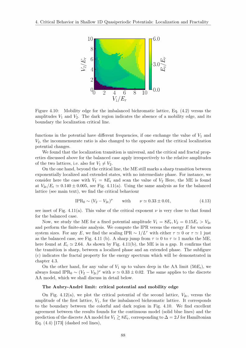
4. Critical Behavior in Shallow 1D Quasiperiodic Potentials: Localization and Fractality
Figure 4.10: Mobility edge for the imbalanced bichromatic lattice, Eq. (4.2) versus theamplitudes V1 and V2. The dark region indicates the absence of a mobility edge, and itsboundary the localization critical line.
functions in the potential have different frequencies, if one exchange the value of V1 andV2, the incommensurate ratio is also changed to the opposite and the critical localizationpotential changes.
We found that the localization transition is universal, and the critical and fractal prop-erties discussed above for the balanced case apply irrespectively to the relative amplitudesof the two lattices, i.e. also for V1 6= V2.
On the one hand, beyond the critical line, the ME still marks a sharp transition betweenexponentially localized and extended states, with no intermediate phase. For instance, weconsider here the case with V1 = 8Er and scan the value of V2 Here, the ME is foundat V2c/Er ' 0.140 ± 0.005, see Fig. 4.11(a). Using the same analysis as for the balancedlattice (see main text), we find the critical behaviour
IPR0 ∼ (V2 − V2c)ν with ν ' 0.33± 0.01, (4.13)
see inset of Fig. 4.11(a). This value of the critical exponent ν is very close to that foundfor the balanced case.
Now, we study the ME for a fixed potential amplitude V1 = 8Er, V2 = 0.15Er > V2cand perform the finite-size analysis. We compute the IPR versus the energy E for varioussystem sizes. For any E, we find the scaling IPR ∼ 1/Lτ with either τ ' 0 or τ ' 1 justas the balanced case, see Fig. 4.11 (b). A sharp jump from τ ' 0 to τ ' 1 marks the ME,here found at Ec ' 2.64. As shown by Fig. 4.11(b), the ME is in a gap. It confirms thatthe transition is sharp, between a localized phase and an extended phase. The subfigure(c) indicates the fractal property for the energy spectrum which will be demonstrated inchapter 4.3.
On the other hand, for any value of V1 up to values deep in the AA limit (50Er), wealways found IPR0 ∼ (V2 − V2c)
ν with ν ' 0.33 ± 0.02. The same applies to the discreteAA model, which we shall discuss in detail below.
The Aubry-André limit: critical potential and mobility edge
On Fig. 4.12(a), we plot the critical potential of the second lattice, V2c, versus theamplitude of the first lattice, V1, for the imbalanced bichromatic lattice. It correspondsto the boundary between the colorful and dark region in Fig. 4.10. We find excellentagreement between the results founds for the continuous model (solid blue lines) and theprediction of the discrete AA model for V1 & 8Er, corresponding to ∆ = 2J for HamiltonianEq. (4.4) [173] (dashed red lines),
88

4. Critical Behavior in Shallow 1D Quasiperiodic Potentials: Localization and Fractality
Figure 4.11: Critical and fractal behaviour for the imbalanced bichromatic lattice. Herewe use V1 = 8.0Er and r = (
√5 − 1)/2. (a) IPR of the ground state, IPR0, versus the
amplitude of the second lattice V2. Darker lines correspond to increasing system sizes,L/a = 50 (light blue), 200 (blue), 1000 (dark blue), 10000 (black). Inset: Same dataversus V2−V2c in log-log scale, confirming the critical behaviour IPR0 ∼ (V2−V2c)
ν , withν ' 0.33 ± 0.01 (dashed red line). (b) Scaling exponent τ versus the energy E as foundfrom fits as IPR ∼ 1/Lτ , for the specific case V2 = 0.15Er > V2c. The black dashed linemarks the ME. (c) Energy box-counting number NB as a function of the energy resolutionε, in the energy window corresponding to panel (b).
Figure 4.12(b) shows the same comparision in the opposite situation where lattice 2is in the tight-binding regime and lattice 1 is weak. In this case, the AA parameters arechanged from Eq. (4.5) by exchanging V1 and V2 and replacing Er by r2Er. they write
J ' 4Err1/2
√π
(V2
Er
)3/4
exp
(−2r−1
√V2
Er
)with ∆ ' V1
2exp
(−r−1
√Er
V2
).
(4.14)Then, the critical potential V1c found in the continuous model approaches the AA predic-tion for V2 & 6Er.
In the AA model, it is well known that there is no ME. However, in the AA limit of thecontinuous model, we find a finite ME. This is due to the fact that the ME is found abovethe lowest band, which is the only one described in the AA model. Thus, the two resultsare actually compatible. In Fig. 4.12(c), we show the lowest part of the energy spectrumin the AA limit of the continuous bichromatic model, V1 = 10Er Er, as a function ofthe amplitude of the second lattice, V2. The structure of the spectrum is reminiscent ofthe band spectrum of the dominant lattice, and we refer to the visible states clusters as
Figure 4.12: Comparison between the critical point found in the continuous bichromaticmodel (solid blue lines) and the discrete Aubry-André model (dashed red lines). Panel (a)corresponds to the tight-binding regime for lattice 1 and panel (b) to tight-binding regimefor lattice 2, respectively. Panel (c) shows the lowest part of the energy spectrum forV1 = 10Er, as a function of V2. The color scale encodes the IPR, corresponding to localized(blue) and extended (yellow) states. The ME is shown as the solid black line.
89

4. Critical Behavior in Shallow 1D Quasiperiodic Potentials: Localization and Fractality
the first bands of the main lattice. The color scale encodes the IPR, corresponding tolocalized (blue) and extended (yellow) states. The solid black line shows the mobility edgeas found from a cut of Fig. 4.10 at the fixed value of V1 = 10Er. For vanishingly smallvalues of V2, there is no ME and all the states are extended. When increasing the value ofV2, the ME sharply jumps to a value in the first band gap of the main lattice. Then, all thestates of the first band of the main lattice become localized. The critical point is found atV2 ' 0.09Er. Using the formulas in Eq. (4.5), we find that it corresponds to ∆/2J ' 1.04,in excellent agreement with the prediction of the discrete AA model [173]. Note that thestates of the second and third bands of the main lattice are still extended. They becomelocalized at a higher value of V2, see Fig. 4.10.
The Aubry-André limit: critical exponent
It is worth noting that the behavior of the IPR differs from that of the Lyapunovexponent (inverse localization length). The IPR is dominated by the core of the wavefunction and characterizes, for instance, the short-range interaction energy of two particlesin a localized state [22]. In contrast, the Lyapunov exponent γ characterizes the exponentialtails of the wave functions,
ψ(x) ∼ exp(−γ|x|), (4.15)
and it is insensitive to the core. For nonpurely exponential wave functions, which appearin our model (see for instance Fig. 4.4(b)), these two quantities are not proportional. Forinstance, in the AA model, one has
γ ∝ ln(∆/2J). (4.16)
At the critical point ∆ = 2J , we can perform the Taylor expansion of the ln function at∆ = 2J and find
γ ∝ ∆−∆c
2J. (4.17)
From Eq. (4.5), we find ∆ ∝ V2 and J is independent of V2, thus we can write
γ ∝ (V2 − V2c)β. (4.18)
with the Lyapunov critical exponent β = 1. This value differs from the IPR criticalexponent-ν ' 1/3-found above.
In order to compare the two behaviors, we plot the ground-state wavefunction forthe AA model slightly above the critical point, namely ∆/J = 2.05, see Fig. 4.13. Thewavefunction shows a clear exponential localization in the wings. The dahsed red lines
Figure 4.13: Ground-state wavefunction of the Aubry-André model for ∆/J = 2.05 (solidblue line) together with exponential fits (dashed red lines) on the left-hand and right-handsides of the localization center.
90

4. Critical Behavior in Shallow 1D Quasiperiodic Potentials: Localization and Fractality
are the fitted exponential function |ψ| ∝ e−γ|x−x0| with the localization center x0 andthe Lyapunov exponent γ as fitting parameters. It yields γ = 6.2 × 10⁻³ ± 6.85 × 10⁻⁵.However, the wavefunction is not a pure exponential function. In particular, it showsa core about one order of magnitude larger than the exponential fit at the localizationcenter x0. This core dominates the IPR. For instance, restricting the wavefunction to therange [x1, x2] such that ψ(x1) = ψ(x2) = 0.01ψ(x0), we find that the IPR is 99.5% of thevalue found for the full wavefunction. Here, we cut at 0.01ψ(x0) since this is where thewavefunction starts to deviate from the exponential decay. Our result illustrated that theIPR is independent of the exponential behaviour of the tails, and the IPR and Lyapunovexponent yield different pieces of information about localization. Moreover, we performthe study of IPR and γ by scanning V2 nearby V2c, see Fig. 4.14. For both of the twoparameters, we find a linear behavior in log-log scale. Fitting them by a linear function,we find the scalings
IPR0 ∼ (V2 − V2c)ν and γ ∼ (V2 − V2c)
β, (4.19)
with ν ' 0.33± 0.015 and β ' 0.96± 0.04.
The trichromatic lattice
Now, we consider the trichromatic lattice
V (x) =V
2
[cos (2k1x) + cos (2k2x+ ϕ) + cos
(2k3x+ ϕ′
) ], (4.20)
with k3/k2 = k2/k1 = r, so that the three lattice spacings are incommensurate to eachother [note that k3/k1 = r2 = (3 −
√5)/2 is an irrational number]. Performing the same
analysis as for the other models, we recover the same universal features. We find a finitecritical amplitude Vc and the critical behavior IPR0 ∼ (V − Vc)
ν with ν ' 0.327 ± 0.007;see Fig 4.6(c). The only significant difference is that the critical point for the trichromaticlattice, Vc/Er ' 0.400±0.005, is smaller than for the bichromatic lattice, see green dashedline in Fig. 4.6(a). In particular, we study the standard deviation of the potential,
∆V =√〈V (x)2〉 − 〈V (x)〉2 (4.21)
which is the quantity that characterizes the amplitude of disorder in truly disorderedsystem. For the quasiperiodic potentials we considered, the term 〈V (x)〉2 in Eq. (4.21) issimply zero. Then, we have ∆V2 '
√1/4V2 for the bichromatic case and ∆V3 '
√3/8V3
Figure 4.14: The ground state IPR and Lyapunov exponent γ for the AA model nearthe transition point ∆c (data points plotted as yellow balls). Here, both of the two plotsare in log-log scale. In both cases, with a linear fit (blue dashed line), we find the slopesν ' 0.33± 0.015 for (a) and β ' 0.96± 0.04 for (b).
91

4. Critical Behavior in Shallow 1D Quasiperiodic Potentials: Localization and Fractality
for the trichromatic case. Taking the ratio of the two values at the critical point, we find
∆V2c
∆V3c=
√2
3
V2c
V3c= 2.27 (4.22)
Comparing with the balanced bichromatic case, it is a factor about 2.27 smaller at thecritical point for the trichromatic lattice. This is consistent with the intuitive expectationthat it should vanish in the disordered case corresponding to an infinite series of cosinecomponents with random phases [186,187].
Up to now, we have checked the localization properties for imbalanced bichromaticlattices, continuous bichromatice lattices in AA limit, as well as trichromatic lattices. Wefind it’s universal that there exists a finite critical potential and ME. Especially, in theAA limit of the continuous model, the ME exists and is above the band considered inthe discrete AA model. Moreover, we find in all cases a critical exponent ν with the valuearound 1/3 which is quite remarkable. There is no explanation yet for this value and it willbe worth understanding it. In the next subsection, we will focus on the fractal property ofthe energy spectrum and study the location of ME.
4.3 The fractality of the energy spectrum
In this section, we study in detail the fractal properties of the energy spectrum created bythe quasiperiodic potential. It helps us understand better the structure of the bands andgaps and the position of the ME. Also, we will benefit from this result when studying themany-body phase diagram (see details in Chapter 5). Therefore, in this section, we firstintroduce the mathematical definition of the fractal as well as the Hausdorff dimension.Then, we perform the box-counting analysis to the energy spectrum of our quasiperiodicsystem and study its fractal dimension. It helps us reach the conclusion that the ME is al-ways in a gap without any intermediate region thanks to the fractal-like spectrum. Finally,we study in detail the property of the fractal dimension, mainly about its dependence onthe potential amplitude and spectrum range.
4.3.1 Fractals and fractal dimension
In mathematics, a fractal is a subset of an Euclidean space for which its dimension issmaller than the geometrical dimension. The main property of the fractal is the so calledself-similarity: it exhibits similar pattern while going to increasingly smaller scale. InFig. 4.15. (a) and (b), we show two typical examples of fractal structure. Figure 4.15.(a)shows the mathematic textbook example: Sierpinski triangle. The black and white regionsstand for the set and empty space. When using a better and better resolution to observethe shape, small holes represented by the white triangles appear. The structure in smallertriangles are always a repetition of themselves in the larger ones. However, fractals existmuch more widely on top of papers and textbooks. The world we live in is beautiful andthere are plenty of approximate self-similar fractals in the nature. The Romanian broccolipresented in Fig. 4.15.(b) is one of them. There are also other good examples such asanimal coloration patterns, DNA structure, rings of Saturn and etc.
On top of the fractal structure mentioned above, they also exist in the structure of phys-ical quantities, for instance, the energy spectrum of the quasiperiod model. In Fig. 4.15.(c),we plot the first 500 eigenstate for the 1D balanced bichromatic lattice with V = 2.0Er,with system size L = 500a. Zooming the first band, we clearly recover the same struc-ture on a smaller scale, see inset plot. This process also applies for the "second and thirdbands", as well as higher level of zooming. Thus, it will be interesting to study further thefractal property for the spectrum of our system.
92

4. Critical Behavior in Shallow 1D Quasiperiodic Potentials: Localization and Fractality
Figure 4.15: Three examples of fractal structures: (a). Sierpinski triangle. (b). Romanianbroccoli. (c). Energy spectrum of the first 500 states for the 1D balanced bichromaticlattice with V = 2.0Er, with system size L = 500a.
Hausdorff dimension and box-counting analysis
An important property of a fractal structure is the fractal dimension. It depicts theshape scale when increasing the resolution in a predictable way. One of the most widelyused method is the box-counting scaling. In this analysis, it defines a resolution box withlinear size ε. Then, we count the minimal number of ε-size boxes needed to cover thefull system, which is called the box-counting number NB. In a perfect self-similar fractalstructure, the scaling of NB(ε) versus the resolution ε is expected to be
NB(ε) ∼ ε−DH , (4.23)
which defines the fractal dimension DH of the energy spectrum. Thanks to the analysis,this quantity is also called box-counting dimension. In strict mathematical definition, itdiffers from the so-called Hausdorff dimension. However, for well-behaved structures, suchas the Sierpinski triangle and the Cantor set, the two values are the same. This is also thecase for all the models we considered in this thesis. Therefore, from now on, we may callit Hausdorff dimension DH although the calculation is based on the box-counting analysis.
A natural way to calculate DH in practice is to detect the scaling by changing theresolution. Decreasing the resolution by a factor of b, one should expect the box-countingnumber will increase with factor of B. It writes
NB(1
bε) = BNB(ε). (4.24)
Combing it with Eq. (4.23), one shall find
DH =log B
log b. (4.25)
In Fig. 4.16, we show several typical examples of box-counting analysis. In each subplots,we show the resolution ε with the corresponding box-counting number NB. In the upperrow, for a one-dimensional line, we find B = b. Thus, the dimension is DH = logb/logb = 1.In the bottom row, similarly, we consider a filled parallelogram and find B = b2. It leadsto DH = logb2/logb = 2. In the intermediate row, we show the analysis for the Sierpinskitriangle. From the left to the right, each time we decrease the resolution by half and thenumber of necessary boxes increases by a factor of 3. It leads to B = blog23. Thus, theHausdorff dimension is
DH =log3
log2= 1.57. (4.26)
Its value is fractional and smaller than the dimension of its Euclidean space (for a triangle,it is 2). This indicates that there exists a repeating self-similar hole structure when zoomingon smaller and smaller resolutions.
93

4. Critical Behavior in Shallow 1D Quasiperiodic Potentials: Localization and Fractality
Figure 4.16: Three typical examples of box-counting analysis: Upper row: One dimen-sional line. Intermediate row: Sierpinski triangle with Hausdorff dimension DH = 1.57.Lower row: Two dimensional parallelogram.
Cantor set
The cantor set is another important example of fractals in mathematics. It is a set ofpoints lying on a single line segment that has a bunch of gapped intervals which presentin a self-similar structure. The construction of a Cantor set is shown in Fig. 4.17. On the0-th level, we start with the interval [0, 1]. Then, for reaching the first level, we delete 1/3of the segment in the middle, (1
3 ,23), which leaves
C1 = [0,1
3] ∪ [
2
3, 1]. (4.27)
Next, for the two remaining segments, we delete the middle 1/3 intervals for both of them,which leads to
C2 = [0,1
9] ∪ [
2
9,1
3] ∪ [
2
3,7
9] ∪ [
8
9, 1]. (4.28)
If we continue this process up to the level of infinity, we finally obtain the Cantor set C.The process of deleting up to the n-th order can also be understood as observing the
set with resolution ε = (1/3)n. Thus, we shall find B = 2n while b = 3n. Therefore, wecan calculate its Hausdorff dimension DH = log2/log3 ' 0.631. It is fractional and smallerthan the dimension of the Euclidean space DE = 1. Thus, it has a fractal structure with
Figure 4.17: The construction process of the classical Cantor set.
94

4. Critical Behavior in Shallow 1D Quasiperiodic Potentials: Localization and Fractality
Figure 4.18: The original figure of the Hofstadter butterfly produced in Ref. [157],
infinite gaps open in a self-similar way. Moreover, one should notice that the Cantor setwe introduced above is the so-called Cantor middle-1/3 set. The definition of a Cantorset can be much more general. During the process of construction, there does not have tobe a single deleted interval and its position is also not necessarily the middle 1/3. Thisis also known as the so-called generalized Cantor set, which can be mapped to the energyspectrum of the quasiperiodic potentials [185,188] (see details later).
AA model and Hofstader butterfly
The energy spectrum of the Aubry-André model has been studied in detail by DouglasR. Hofstadter in Ref. [157], known for the famous Hofstadter butterfly. Although itsinitial motivation was to study the Harper equation for 2D electrons in magnetic fields,the Schrodinger equation can be mapped onto the AA model as Eq. (4.4) with J = 2∆.The parameter r also stands for the magnetic flux per cell in the 2D problem. In Fig. 4.18,we show the original figure of the famous Hofstadter butterfly in Ref. [157]. It shows aninteresting fractal structure. The horizontal axis is the eigenenergy, while the vertical axisis the ratio of the two lattice spacing r. When r = p/q is rational, the spectrum containsq subbands. When r is irrational, the spectrum is fractal-like and it has a well-definedfractal dimension [189,190].
In fact, when r is irrational, the spectrum is always a fractal, irrespective of the valuefor J/∆. It is always homeomorphic to a Cantor set. This can be understood by therational approximation for an irrational number. We take the golden ratio r = (
√5− 1)/2
as an example. It can always be approximated by the ratio of two neighbours in theFibonacci series Fn, i.e. r ' Fn/Fn+1. On the n-th order of approximation, we find thatthe spectrum contains Fn+1 subbands and Fn+1−1 gaps which opens by the beating of thetwo quasimomentums Fn and Fn+1. Increasing the approximation order n of the irrationalnumber r, more gaps open and it similarly reproduces the construction of a Cantor set. Forthis choice of r, it has even been proved that the fractal dimension for the energy spectrumat J = 2∆ is DH = 0.5 [189, 190]. For other incommensurate number which is not aLiouville number, one can always build the corresponding generalised Fibonacci seriesand perform the similar construction [185, 188].. Even for the continuous quasiperiodicsystem we studied, we argue that the statement still holds and we shall find the fractal-likestructure in the energy spectrum.
95
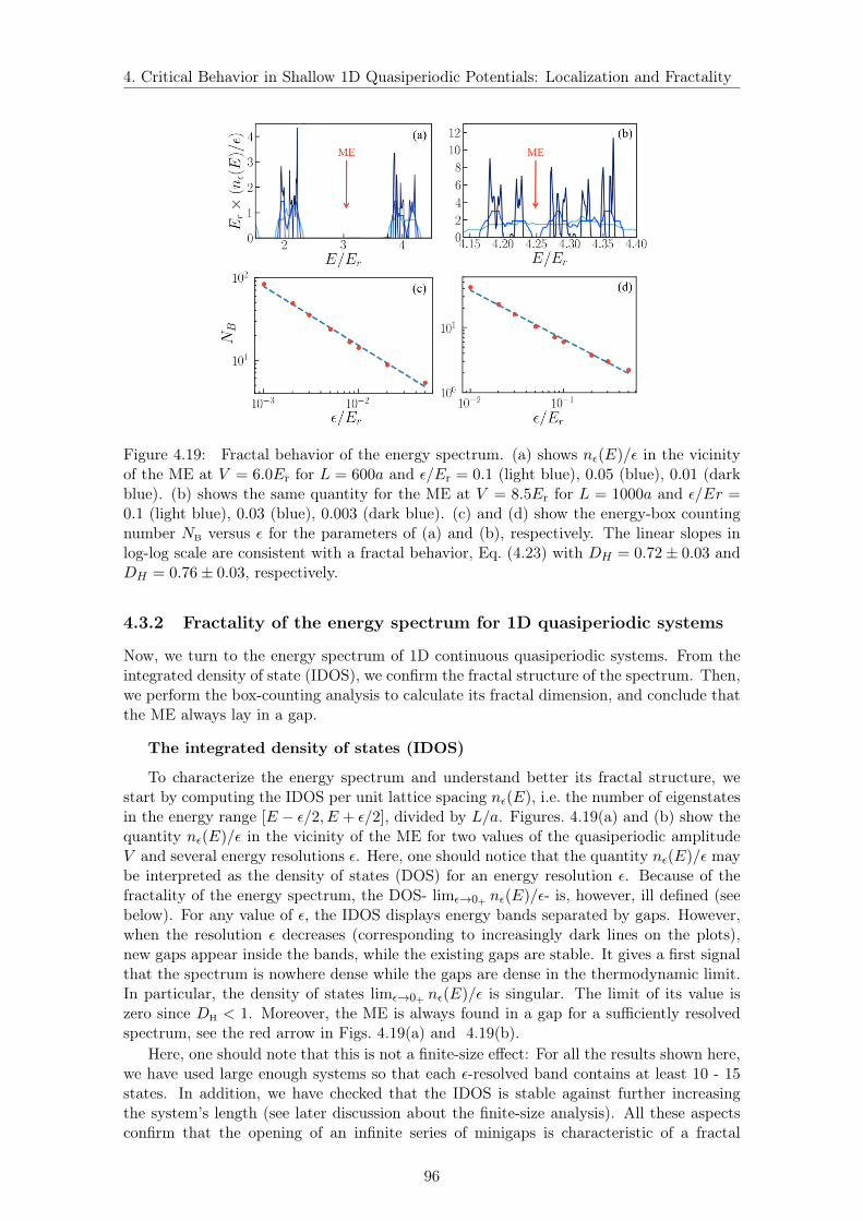
4. Critical Behavior in Shallow 1D Quasiperiodic Potentials: Localization and Fractality
Figure 4.19: Fractal behavior of the energy spectrum. (a) shows nε(E)/ε in the vicinityof the ME at V = 6.0Er for L = 600a and ε/Er = 0.1 (light blue), 0.05 (blue), 0.01 (darkblue). (b) shows the same quantity for the ME at V = 8.5Er for L = 1000a and ε/Er =0.1 (light blue), 0.03 (blue), 0.003 (dark blue). (c) and (d) show the energy-box countingnumber NB versus ε for the parameters of (a) and (b), respectively. The linear slopes inlog-log scale are consistent with a fractal behavior, Eq. (4.23) with DH = 0.72± 0.03 andDH = 0.76± 0.03, respectively.
4.3.2 Fractality of the energy spectrum for 1D quasiperiodic systems
Now, we turn to the energy spectrum of 1D continuous quasiperiodic systems. From theintegrated density of state (IDOS), we confirm the fractal structure of the spectrum. Then,we perform the box-counting analysis to calculate its fractal dimension, and conclude thatthe ME always lay in a gap.
The integrated density of states (IDOS)
To characterize the energy spectrum and understand better its fractal structure, westart by computing the IDOS per unit lattice spacing nε(E), i.e. the number of eigenstatesin the energy range [E − ε/2, E + ε/2], divided by L/a. Figures. 4.19(a) and (b) show thequantity nε(E)/ε in the vicinity of the ME for two values of the quasiperiodic amplitudeV and several energy resolutions ε. Here, one should notice that the quantity nε(E)/ε maybe interpreted as the density of states (DOS) for an energy resolution ε. Because of thefractality of the energy spectrum, the DOS- limε→0+ nε(E)/ε- is, however, ill defined (seebelow). For any value of ε, the IDOS displays energy bands separated by gaps. However,when the resolution ε decreases (corresponding to increasingly dark lines on the plots),new gaps appear inside the bands, while the existing gaps are stable. It gives a first signalthat the spectrum is nowhere dense while the gaps are dense in the thermodynamic limit.In particular, the density of states limε→0+ nε(E)/ε is singular. The limit of its value iszero since DH < 1. Moreover, the ME is always found in a gap for a sufficiently resolvedspectrum, see the red arrow in Figs. 4.19(a) and 4.19(b).
Here, one should note that this is not a finite-size effect: For all the results shown here,we have used large enough systems so that each ε-resolved band contains at least 10 - 15states. In addition, we have checked that the IDOS is stable against further increasingthe system’s length (see later discussion about the finite-size analysis). All these aspectsconfirm that the opening of an infinite series of minigaps is characteristic of a fractal
96

4. Critical Behavior in Shallow 1D Quasiperiodic Potentials: Localization and Fractality
Figure 4.20: Two examples of the box-counting number NB for the energy spectrum underdifferent resolutions ε.
behavior.
Box-counting analysis for the energy spectrum
As we mentioned in the last subsection, the fractal character of the energy spectrum of1D incommensurate systems has been studied for discrete models, such as the Fibonaccichain and the AA model [157, 161, 189–192]. In all of these cases, it was shown that thespectrum is homeomorphic to a Cantor set. To study fractality in our continuous model,we use the direct box-counting analysis similar as the mathematical one [193, 194]: Weintroduce the energy-box counting number,
NB(ε) = limq→0+
∫ E2
E1
dE
ε
[nε(E)
]q, (4.29)
for some energy range [E1, E2]. In the limit q → 0+, the quantity[nε(E)
]q approaches 1 ifnε(E) 6= 0 and 0 if nε(E) = 0. Therefore, the quantity limq→0+
[nε(E)
]q contributes 1 inthe boxes of width ε containing at least one state and vanishes in the empty boxes. Thesum of these contributions, NB(ε), counts the minimal number of ε-wide boxes necessaryto cover all the states within the energy range [E1, E2]. In Fig. 4.20, we show two typicalexamples of the box-counting number NB under different observation resolution ε. InFig. 4.20 (b), there are 8 boxes in the whole energy range but only NB = 7 filled box, sincethe third box from the bottom contains no eigenstate inside.
The scaling of NB(ε) versus the energy resolution ε will follow Eq. (4.23), which definesthe Hausdorff dimension DH of the energy spectrum. In all considered cases, we found ascaling consistent with Eq. (4.23) with 0 < DH < 1. This is characteristic of a nontrivialfractal. For a continuous (respectively discrete) spectrum, one finds DH = 1 (respectively0). Intermediate values of DH are characteristic of a nontrivial self-similar behavior. Forinstance Figs. 4.19(c) and (d) show NB versus ε in the vicinity of the MEs at V = 6Erand V = 8.5Er for the energy ranges corresponding to Figs. 4.19(a) and (b), respectively.We find a linear scaling in the log-log scale, consistent with Eq. (4.23) and the Hausdorffdimensions DH = 0.72 ± 0.03 and DH = 0.76 ± 0.03, respectively. Both values are signifi-cantly smaller than the geometrical dimension d = 1. Therefore, the Lebesgue measure ofthe energy support vanishes in the limit of an infinitely small resolution, and the spectrumis nowhere dense in the thermodynamic limit.
In the section 4.2.1, we have questioned whether the location of ME is a gap or a band.Thanks to the fractality of the spectrum, all the points in the spectrum are disconnectedwith each other. Therefore, there is even no connected band exists in the spectrum in thethermodynamic limit. And it confirms that the ME should always lie in a gap.
97

4. Critical Behavior in Shallow 1D Quasiperiodic Potentials: Localization and Fractality
Figure 4.21: Two examples of the box-counting number NB for the energy spectrum underdifferent resolutions ε. (a). 1D trichromatic lattice with V = 0.6Er. (b) 2D quasicrystalstructure with V0 = 5.5Er.
Here, we should note that the Hausdorff dimension found above significantly differs fromthat found in previous work at the critical point of the AA model, DH ' 0.5 [189, 190].We conclude that the spectral Hausdorff dimension is a nonuniversal quantity. This isconfirmed by further calculations we performed. For instance, in the AA limit of ourcontinuous model, V1 V2, Er, we recover DH = 0.507 ± 0.005 at the critical point.Conversely, we found DH = 0.605 ± 0.014 at the critical point of the balanced lattice.However, we argue that the existence of the fractal spectrum structure and DH < 1 isuniversal. It holds for any 1D bichromatic lattices. We even confirm further that it holdsfor the spectrum of 1D trichromatic lattices and 2D quasiperiodic lattices. In Fig. 4.21,we show the box-counting number versus the resolution ε for the energy spectrums of twotypical cases. In Fig. 4.21(a), we study the case of the 1D trichromatic lattice as Eq. (4.20)with V = 0.6Er. Here, we find a linear behavior in log-log scale with the fractal dimensionDH = 0.74± 0.02. Also, in Fig. 4.21(b), we treat the 2D quasicrystal structure consideredin Refs. [19,33,195], which Hamiltonian writes
H =∑j
[− ~2
2m∇2j + V (rj)
](4.30)
where rj is the position of the j-th particle and V (r) quasicrystal lattice potential. Thequasicrystal potential is eightfold rotation symmetric,
V (r) = V0
4∑k=1
cos2 (Gk · r) (4.31)
where V0 is the potential amplitude and the quantities Gk are the lattice vectors of fourmutually incoherent standing waves oriented at the angles 0, 45, 90, and 135, respec-tively. We perform the similar exact diagonalization techniques as for the 1D case, for thepotential V0 = 5.5Er to find the energy spectrum and perform the box-counting analysis toget Fig. 4.21(b). Even in this case, we find a linear behavior in log-log scale and a fractaldimension DH = 0.83± 0.03.
Finite-size analysis and check of fidelity
Here, we want to show that the opening of mini gaps in the energy spectrum, i.e. theresults shown in Figs. 4.19(a) and (b) are not due to finite-size effects. We have computedthe integrated density of states (IDOS) for various system lengths. Figures 4.22(a) and(b) reproduce the IDOS shown on Fig. 4.19 for the smallest considered energy resolutionsε and various values of the length L. The results corresponding to the different systemlengths are indistinguishiable. Moreover, we have computed the Hausdorff dimensions in
98

4. Critical Behavior in Shallow 1D Quasiperiodic Potentials: Localization and Fractality
Figure 4.22: Finite-size scaling analysis for the IDOS. The panels (a) and (b) reproducethe IDOS divided by the energy resolution, nε(E)/ε, shown on Fig. 2 for the smallestconsidered energy resolutions ε but for various values of the length L. (a) IDOS in thevicinity of the ME at V = 6Er for ε = 0.01Er and L = 400a (dotted light blue line),600a (dashed blue line), 800a (solid black line). (b) Same as panel (a) for V = 8.5Er,ε = 0.003Er, and L = 800a (dotted light blue line), 1000a (dashed blue line), 1200a (solidblack line). (c) and (d) Hausdorff dimension DH calculated for the various system sizesused for the panels (a) and (b).
both cases for the different lengths, see Figs. 4.22(c) and (d). The behaviours of DH donot show significant variations with the system size. These results allow us to rule outfinite-size effects.
Furthermore, we want to confirm the fidelity of our box-counting approach, we haveperformed two additional checks. On the one hand, we have computed the Hausdorffdimension of the first band of the first lattice for the continuous model in the Aubry-André limit (V1 V2, Er). At the critical point, we find a clear fractal behaviour of theenergy-box number, NB ∼ ε−DH with DH = 0.51± 0.01, see Fig. 4.23(a). It is in excellent
Figure 4.23: Energy-box counting number NB versus ε for (a) the continuous bichromaticmodel in the Aubry-André limit, V1 = 10Er and V2 = 0.09Er, at criticality and (b) thecommensurate bichromatic lattice, r = 2/3 and V1 = V2 = 6Er.
99

4. Critical Behavior in Shallow 1D Quasiperiodic Potentials: Localization and Fractality
Figure 4.24: Fractal dimension of the energy spectrum for various values of V1 and V2.The black dashed line is the critical potential calculated in Ref. [86]
agreement with the Hausdorff dimension found by another method in the discrete Aubry-André model, DH ' 0.5 [189, 190]. On the other hand, we have reproduced the samecalculations as for the case corresponding to Fig. 4.22(b), i.e. V1 = V2 = 6Er, but with thecommensurate filling r = 2/3. It corresponds to a periodic system and a regular spectrumwith DH = 1 is expected. The result is shown on Fig. 4.23(b) and we find DH = 0.98±0.01,in excellent agreement with this prediction. These results further validate our approach todetermine the fractal dimension of the energy spectrum.
4.3.3 Properties of the spectrum fractal dimension
As we explained in the previous subsection, the existence of a spectrum fractal dimensionsmaller than unity is universal for quasiperiodic potentials with finite potential amplitudes.However, its value is not universal and will change with the potentials. In this subsection,we study in detail the property of the spectrum fractal dimension, i.e. its dependence onthe quasiperiodic potentials.
We focus on the energy spectrum in the range [E0, EN ], where E0 is the ground stateenergy and EN is the energy of the N -th state with N = L/a. For the following calcula-tions, we take N = 500. Here, we scan V1 and V2 and calculate the fractal dimension DH ofthe energy spectrum. For both of the two values V1 and V2, we scan from 0Er to 6Er, withresolution of 0.25Er. The results are shown in Fig. 4.24. From the results, we find thatwhen (V1, V2) is very small or large, DH are going to unity. The physical interpretation isthe following. In the zero potential limit, we find the spectrum of a free particle which iscontinuous parabola. In the large potential limit, the system is like isolated deep wells withdifferent depth. The eigenenergies are simply the energy of each well. Thus, consideringthe thermodynamic limit L → ∞, the eigenenergies go through all the values between,roughly, [−V1 − V2, V1 + V2], and it should also be continuous and leads to DH = 1. Inbetween, a non-monotonic behavior is presented. The minimum seems appearing at thecritical potential (black dashed line).
To further check the position of the minimum fractal dimension, we plot two cuts ofFig. 4.24, for the two cases: (i) V1 = V2 = V , (ii) V2 = 10Er and scanning V1, see Fig. 4.25(a) and (b) correspondingly. In both cases, we find the fractal dimension tends to unity inthe zero and large potential limits. Also, a minimum value of DH is found approximately atthe position of Vc. Especially, for the case (ii), we find the minimum valueDH = 0.51±0.02,which recovers the prediction of the Aubry-André model in Refs. [189,190]. Although the
100
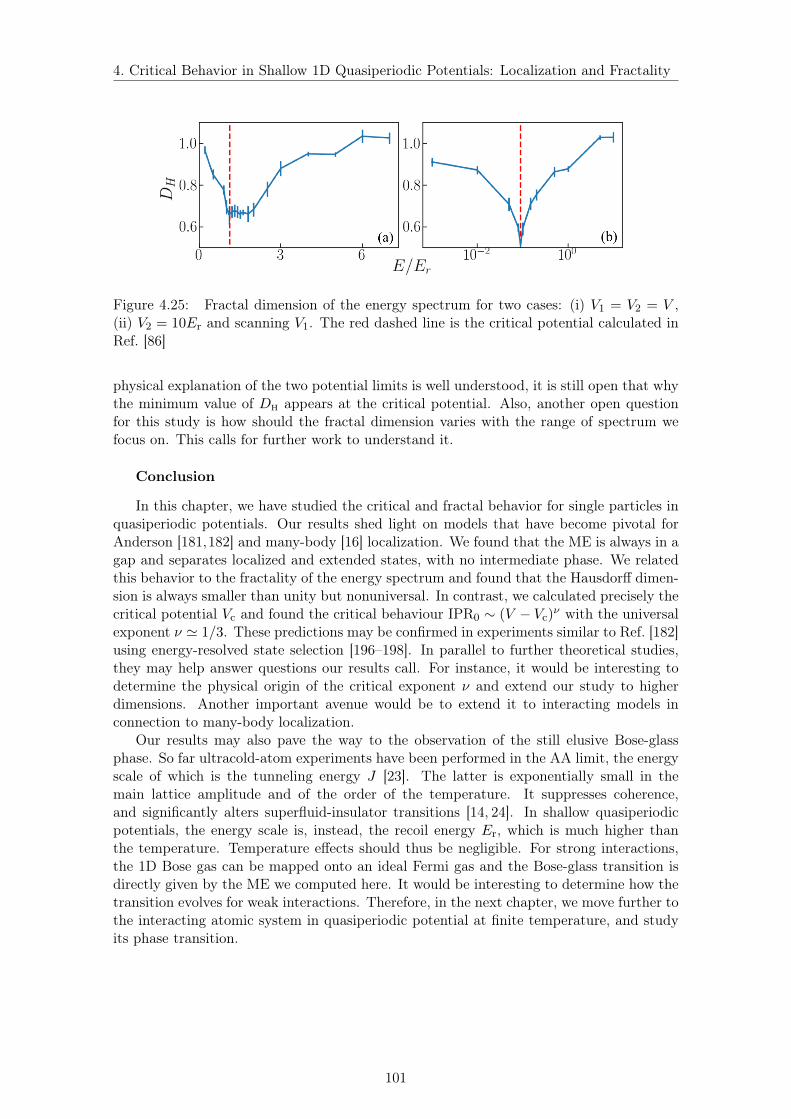
4. Critical Behavior in Shallow 1D Quasiperiodic Potentials: Localization and Fractality
Figure 4.25: Fractal dimension of the energy spectrum for two cases: (i) V1 = V2 = V ,(ii) V2 = 10Er and scanning V1. The red dashed line is the critical potential calculated inRef. [86]
physical explanation of the two potential limits is well understood, it is still open that whythe minimum value of DH appears at the critical potential. Also, another open questionfor this study is how should the fractal dimension varies with the range of spectrum wefocus on. This calls for further work to understand it.
Conclusion
In this chapter, we have studied the critical and fractal behavior for single particles inquasiperiodic potentials. Our results shed light on models that have become pivotal forAnderson [181,182] and many-body [16] localization. We found that the ME is always in agap and separates localized and extended states, with no intermediate phase. We relatedthis behavior to the fractality of the energy spectrum and found that the Hausdorff dimen-sion is always smaller than unity but nonuniversal. In contrast, we calculated precisely thecritical potential Vc and found the critical behaviour IPR0 ∼ (V − Vc)
ν with the universalexponent ν ' 1/3. These predictions may be confirmed in experiments similar to Ref. [182]using energy-resolved state selection [196–198]. In parallel to further theoretical studies,they may help answer questions our results call. For instance, it would be interesting todetermine the physical origin of the critical exponent ν and extend our study to higherdimensions. Another important avenue would be to extend it to interacting models inconnection to many-body localization.
Our results may also pave the way to the observation of the still elusive Bose-glassphase. So far ultracold-atom experiments have been performed in the AA limit, the energyscale of which is the tunneling energy J [23]. The latter is exponentially small in themain lattice amplitude and of the order of the temperature. It suppresses coherence,and significantly alters superfluid-insulator transitions [14, 24]. In shallow quasiperiodicpotentials, the energy scale is, instead, the recoil energy Er, which is much higher thanthe temperature. Temperature effects should thus be negligible. For strong interactions,the 1D Bose gas can be mapped onto an ideal Fermi gas and the Bose-glass transition isdirectly given by the ME we computed here. It would be interesting to determine how thetransition evolves for weak interactions. Therefore, in the next chapter, we move further tothe interacting atomic system in quasiperiodic potential at finite temperature, and studyits phase transition.
101

Chapter 5
Lieb-Liniger bosons in a shallowquasiperiodic potential
Based on the study in the last chapter, we now turn to the Lieb-Liniger bosons in a shallowquasiperiodic lattices in presence of a finite interaction and a finite temperature. The maininterest for investigating such kinds of systems is the interplay between interactions anddisorder, which induces a rich physics. This is at the origin of many intriguing phenomena,including many-body localization [199–203], collective Anderson localization [41, 46–51,149], and the emergence of new quantum phases. For instance, a compressible insulator,known as the Bose glass (BG) [52–54, 83, 204], may be stabilized against the superfluid(SF) and, in lattice models, against the Mott insulator (MI).
In one-dimensional (1D) systems, it is particularly fascinating for the SF may be desta-bilized by arbitrary weak perturbations, an example of which is the pinning transition inperiodic potentials [3, 13, 15, 72, 205]. Similarly, above an interaction threshold, the BGtransition can be induced by arbitrary weak disorder [52, 53]. The phase diagram of 1Ddisordered bosons has been extensively studied and is now well characterized theoreti-cally [22, 83, 84, 204, 206, 207]. The experimental observation of the BG phase remains,however, elusive [20, 168, 208–211], despite recent progress using ultracold atoms in thetight-binding quasiperiodic potentials [14,24].
Controlled quasiperiodic potentials, as realized in ultracold atom [153, 163, 212] andphotonic [160,161,213,214] systems, have long been recognized as a promising alternative toobserve the BG phase. So far, however, this problem has been considered only in the tight-binding limit, known as the Aubry-André model [23, 164, 165, 192, 215]. It sets the energyscale to the tunneling energy, which is exponentially small in the main lattice amplitude andof the order of magnitude of the temperature in typical experiments. The phase coherenceis then strongly reduced, which significantly alters the phase diagram. Although suchsystems give some evidence of a Bose glass phase [14, 24], they require a heavy heuristicanalysis of the data to factor out the very important effects of the temperature. Thus,we propose to overcome this issue by using shallow quasiperiodic potentials. The energyscale would then be the recoil energy, which is much larger than typical temperatures inultracold-atom experiments [1, 212]. This, however, raises the fundamental question ofwhether a BG phase can be stabilized in this regime: In the hard-core limit, interactingbosons map onto free fermions [40] (see detail discussion in Chapter 1). A band of localized(resp. extended) single particles then maps onto the BG (resp. SF) phase while a band gapmaps onto the MI phase. In the shallow bichromatic lattice, however, we have shownthat band gaps, i.e. MI phases, are dense [86] and the BG would thus be singular, seedetailed discussions about the fractality of the single-particle spectrum in Section 4.3.On the other hand, decreasing the interactions down to the meanfield regime favors theSF phase [22, 52, 53, 216]. Hence, a BG can only be stabilized, if at all, for intermediate
102

5. Lieb-Liniger Bosons in a Shallow Quasiperiodic Potential
Figure 5.1: Phase diagrams of Lieb-Liniger bosons in a shallow quasiperiodic potential forincreasing values of the potential (V = Er < Vc, V = 1.5Er & Vc, and V = 2Er > Vc fromleft to right). Upper row: Quantum phase diagrams as found from QMC calculations at avanishingly small temperature [kBT = 10−3Er for (a1) and kBT = 2× 10⁻³Er for (a2) and(a3)]. Lower row: Counterpart of the upper row at the finite temperature kBT = 0.015Er.There, the "SF", "MI", and "BG" regimes are defined as those that retain the zero-temperature properties of the corresponding phases. The normal fluid (NF) correspondsto points where significant temperature effects are found. On the left of each panel, weshow the equation of state ρ(µ) at strong interactions, −a1D/a = 0.05 (solid black line)together with that of free fermions at the corresponding temperatures (dashed red line).Note that the smallest band gaps are smoothed out by the finite temperatures. The dottedblue line visible on panel (a2) shows the single-particle ME at V = 1.5Er, Ec ' 0.115Er.
interactions.
In this chapter, we tackle this issue using exact quantumMonte Carlo calculations [217].Firstly, we briefly review the previous studies of the BG transition in the disordered systemas well as the Aubry-André model. Then, we move to the computation of the exact phasediagram of interacting bosons in a shallow 1D bichromatic lattice. Our main results aresummarized on Fig. 5.1 and we will give detailed discussion for it in Section 5.2. Weshall see that a BG phase can be stabilized at intermediate interaction for a quasiperiodicpotential above a critical threshold. Finally, we will study the finite temperature effect andwe shall show that the BG phase is robust to the thermal fluctuations up to temperaturesaccessible to present-day experiments.
5.1 The Bose glass phase
Before addressing the problem of the phase diagram for 1D shallow quasiperiodic systems,we briefly review previous work and basic knowledge about the Bose glass. We start withthe first waves of demonstration for Bose glass phase in purely disordered systems [52–54].Then, we talk about the Bose glass physics in the Aubry-André model [23,164,165,192,215],and its experimental achievements [14,20,24].
103

5. Lieb-Liniger Bosons in a Shallow Quasiperiodic Potential
Figure 5.2: The Bose-Hubbard model. (a). The illustration of its potential. (b). Thephase diagram.
5.1.1 Bose glass phase in random potentials
The first work on the Bose glass is in Refs. [52, 53]. It is specific to one dimensionalcontinuous systems in the presence of disorder and use renormalization group analysiswithin Luttinger liquid approach. Then, in Ref. [54], M. P. A. Fisher et al consider thedisordered Bose-Hubbard model. For 1D bosons in continuum, it is in superfluid phase atzero temperature. In presence of a disordered potential, however, a Bose glass phase mayappear against the SF phase when the disorder is large enough. On the one hand, it islocalized thanks to the disorder. On the other hand, adding one particle only cost a smallamount of energy, i.e. it is compressible. Therefore, with the competition between disorderand interaction, the BG phase can be stabilized against SF in certain regimes. Moving tothe lattice system, the argument is similar, except that the BG phase appears in betweenthe Mott insultor and superfluid. In the following, we present the introduction of the Boseglass phase in disordered lattice model following the statement in Ref. [54], the main ideaof which is the minimization of energy for Bose-Hubbard model. One may notice that anequivalent statement is illustrated in Ref. [53] from the renormalization group aspect.
The Bose-Hubbard model
We start with the Bose-Hubbard model which is created by an external periodic lat-tice potential, shown in Fig. 5.2.(a). In this case, we expect Mott insulator lobes instrongly-interacting regime which turns into superfluid phase while interaction decreases,as discussed in section 1.3. In this case, the Hamiltonian writes
H = −J∑i,j
a†i aj +U
2
∑i
ni(ni − 1)− µ∑i
ni (5.1)
with J the tunneling, U the on-site interaction and µ the chemical potential. To obtainthe quantum phase diagram at zero temperature, one should minimize the total energy.Equivalently, thanks to the periodicity, we simply minimize the on-site energy on eachlattice sites. We first consider the atomic limit J = 0. Then, the on-site energy of latticesite i writes
ei =1
2Uni(ni − 1)− µni, (5.2)
which is a parabolic function of ni. Thus, for a certain µ in the range U(n− 1) < µ < Unwith n a certain integer, taking ni = n will minimize the energy ei. Equivalently, it meansthe system has a fixed integer fillings in each lattice sites, which forms the incompressibleMott-insulator phase.
104

5. Lieb-Liniger Bosons in a Shallow Quasiperiodic Potential
Figure 5.3: The Bose-Hubbard model with on-site disorder. (a). The illustration of itspotential. (b). The phase diagram.
Now, we take a finite tunneling parameter J > 0. It is important to introduce twotypical energies,
δEp ∼ (1
2− α)U, δEh ∼ (
1
2+ α)U (5.3)
which are the energies required to add or remove one particle from the system. Let’sconsider starting from a point in the µ−J plane with n particle on each site. Allowing oneparticle to hop from one site to its neighbour will gain approximately J in kinetic energywith the expense of δEph = δEp + δEh in the interaction energy. Thus, when J is smallenough compared to the scale of δEph, the system will remain in the Mott insulator phasewith filling n. For each fixed µ, when J is large enough compared to δEph and above acritical value (J/U)c, the filling ni = n doesn’t give the minimal energy any more. Eachparticle are delocalized on the full system and thus it forms a compressible and extendedsuperfluid phase. Combining the above statements, we shall find the phase diagram inFig. 5.2.(b).
Bose-Hubbard model with disorder
Now, we add the disorder on top of the Bose-Hubbard model, see Fig. 5.3.(a). With thepresence of disorder, a localized but compressible Bose glass phase is expected to appearin between the MI and SF phase. Here, the Hamiltonian shall write
H = −J∑i,j
a†i aj +U
2
∑i
ni(ni − 1)−∑i
(µi + δµi)ni (5.4)
with δµi the on-site disorder. It’s a random number following the uniform distributionbetween [−∆,∆]. Hence, in the atomic limit, the on-site energy of lattice site i shouldbecome
ei =1
2Uni(ni − 1)− (µ+ δµi)ni. (5.5)
We assume the disorder term ∆ is smaller than the interaction term U . Starting withJ = 0, for minimizing the on-site energy, there are three possibilities. They yield:
• For n − 1 < µ/U < n − 1 + ∆, the on-site energy might be minimized by eitherni = n− 1 or ni = n.
• For n− 1 + ∆ < µ/U < n−∆, the on-site energy will be minimized by ni = n.
• For n −∆ < µ/U < n, the on-site energy might be minimized by either ni = n orni = n+ 1.
105

5. Lieb-Liniger Bosons in a Shallow Quasiperiodic Potential
Figure 5.4: The phase diagram for bichromatic Bose-Hubbard model shown in Ref. [23].The diagrams are shown as a function of the interaction U and quasiperiodic potentialamplitude V2, in the unit of the hopping J . The indicated phases are Bose glass (BG),superfluid (SF), Mott insulator (MI) and incommensurate charge density wave (ICDW).The three plots corresponds to three particle densities: (a). n = 1, (b). n = r, (c) n = 0.5.For the case n = 1, the darker region indicates there could be small gaps which cannot beresolved by the calculation.
For the second case above, all the lattice sites have the same integer filling ni = n, andit thus forms a Mott insulator phase. The width of the Mott insulator lobe writes ∆µ =U − 2∆. However, for the first and third cases, different lattice sites might be minimizedby different values of the filling. Thusr, the many-body state is localized globally and theaverage filling is not an integral. Thus, it is neither a Mott insulator nor a superfluid.It is a compressible insultator phase with fractional fillings, which we called Bose glass.Then, for J > 0, similar as the periodic system case, when J U , it’s insufficient toovercome the repulsive on-site potential and allow extra particles to hop in the system.Then, for each fixed µ, the system go through a transition to the superfluid phase whenJ is sufficiently large. Moreover, even for the BG phase, the finite tunneling enables theparticles to hop between different sites and enhances the coherence of the system. Abovea certain value (J/U)c, the system becomes extended and it turns to the superfluid phase.Therefore, the phase diagram should look like Fig. 5.3.(b). Moreover, when the disorder islarge enough ∆ > 2U , the Mott lobe are totally eliminated and there should only remainthe BG and SF phases in the phase diagram.
5.1.2 Bose glass phase in quasiperiodic Bose-Hubbard model
In this part, we shall introduce the known work of Bose glass physics in quasiperiodicsystems. All the following work is done in the tight-binding limit, i.e. the Aubry-Andrémodel, and it contains research both theoretically and experimentally.
Theoretical prediction of the phase diagram
The system we consider now is a Lieb-Liniger gas, i.e. a 1D N -bosons gas with re-pulsive contact interactions, subjected to a quasiperiodic potential V (x). We recall theHamiltonian writes
H =∑
1≤j≤N
[− ~2
2m
∂2
∂x2j
+ V (xj)]
+ g∑j<`
δ(xj − x`), (5.6)
where m is the particle mass, x is the space coordinate, and g = −2~2/ma1D is theinteraction strength with a1D < 0 the 1D scattering length. The quasiperiodic potential
106

5. Lieb-Liniger Bosons in a Shallow Quasiperiodic Potential
writesV (x) = V1 cos2 (k1x) + V2 cos2 (k2x+ ϕ) . (5.7)
where the spatial frequencies k1 and k2 are incommensurate. The corresponding recoilenergy is defined as Erj = ~2k2
j /2m with j = 1, 2.Now, we introduce the theoretical outcome from Ref. [23] for the tight-binding limit,
which is named as bichromatic Bose-Hubbard model. The considered situation satisfiesthe condition
V1 V2, Er1, Er2. (5.8)
It is similar as the one for the non-interacting Aubry-André model. On the one hand, thepotential V1 is much larger than the recoil energy, the system is thus in the tight-bindinglimit and can be treated as discretized. On the other hand, the second lattice V2 is muchsmaller than the first one, which can be treated as a pertubation. Following the derivationin Ref. [23], one can recover the discrete version of the tight-binding Hamiltonian, whichyields
H = −J∑j
[b†j+1bj + h.c.] + U∑j
nj(nj − 1)/2 +V2
2
∑j
[1 + cos(2rπj + 2φ)]nj (5.9)
with b†j the creation operator of bosons and nj = b†jbj the local particle number operator.The hopping term J and interaction term U follows the same definition as in the non-interacting Aubry-André model, see section 4.1.
With Density Matrix Renormalization Group (DMRG) calculations, one can calculatethe phase diagram at finite interactions and zero temperature. In Fig. 5.4, they show thephase diagrams of three typical cases. In each plot, they show the result for a fixed densityn at different interaction U and disorder V2, rescaled by the hopping J . For obtainingthe phase, the numerics are performed to calculate five quantities, namely the one-bodycorrelation length ξ (see detailed definition in later discussion), the one-particle gap ∆c,the condensate fraction fc, the superfluid density ρs and the Luttinger parameter K. Theverification of the different phases are identified as follows.
Phase ξ ∆c fc ρs K
SF ' L = 0 0 > 0 > 0
MI L > 0 & 0 = 0 = 0
BG L = 0 & 0 = 0 = 0
ICWD L > 0 & 0 = 0 = 0
Table 5.1: Identification of the quantum phases from the DMRG calculations.
Here, from the first two columns of Table. 5.1, we can see that the first three phases canbe distinguished by the correlation length ξ and the one-particle gap ∆. The correlationfunction is algebraic decaying in the SF phase and ξ is thus infinite. For a finite size systemof size L, we would thus have ξ ∼ L, For the other phases, the correlation function decaysexponentially and ξ is finite and smaller than L. Then, the MI and ICWD phase are gappedinsulator with finite ∆ while the SF and BG are gapless. For further distinguishing the MIand ICWD, one should look at the particle filling n. It’s an integer for MI and fractionalnumber for ICWD. The other three columns in Table. 5.1, give redundant information. Onthe one hand, they can be used as a double check for the different phases. On the otherhand, they all have specific physical meanings which describes one aspect of features forthe system.
In Fig. 5.5, we show the calculated results for these quantities for the case n = 1, withthe quantity equals to zero (finite value) while the color of the region is black (non black
107
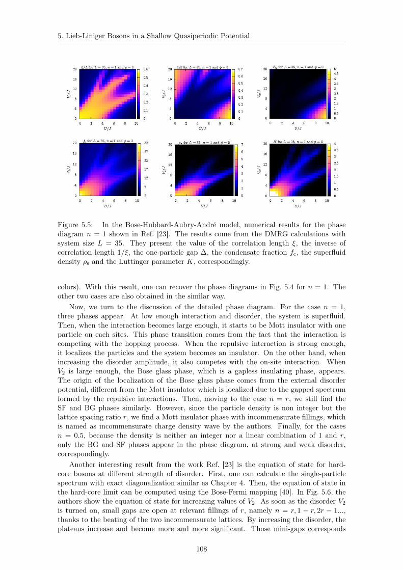
5. Lieb-Liniger Bosons in a Shallow Quasiperiodic Potential
Figure 5.5: In the Bose-Hubbard-Aubry-André model, numerical results for the phasediagram n = 1 shown in Ref. [23]. The results come from the DMRG calculations withsystem size L = 35. They present the value of the correlation length ξ, the inverse ofcorrelation length 1/ξ, the one-particle gap ∆, the condensate fraction fc, the superfluiddensity ρs and the Luttinger parameter K, correspondingly.
colors). With this result, one can recover the phase diagrams in Fig. 5.4 for n = 1. Theother two cases are also obtained in the similar way.
Now, we turn to the discussion of the detailed phase diagram. For the case n = 1,three phases appear. At low enough interaction and disorder, the system is superfluid.Then, when the interaction becomes large enough, it starts to be Mott insulator with oneparticle on each sites. This phase transition comes from the fact that the interaction iscompeting with the hopping process. When the repulsive interaction is strong enough,it localizes the particles and the system becomes an insulator. On the other hand, whenincreasing the disorder amplitude, it also competes with the on-site interaction. WhenV2 is large enough, the Bose glass phase, which is a gapless insulating phase, appears.The origin of the localization of the Bose glass phase comes from the external disorderpotential, different from the Mott insulator which is localized due to the gapped spectrumformed by the repulsive interactions. Then, moving to the case n = r, we still find theSF and BG phases similarly. However, since the particle density is non integer but thelattice spacing ratio r, we find a Mott insulator phase with incommensurate fillings, whichis named as incommensurate charge density wave by the authors. Finally, for the casesn = 0.5, because the density is neither an integer nor a linear combination of 1 and r,only the BG and SF phases appear in the phase diagram, at strong and weak disorder,correspondingly.
Another interesting result from the work Ref. [23] is the equation of state for hard-core bosons at different strength of disorder. First, one can calculate the single-particlespectrum with exact diagonalization similar as Chapter 4. Then, the equation of state inthe hard-core limit can be computed using the Bose-Fermi mapping [40]. In Fig. 5.6, theauthors show the equation of state for increasing values of V2. As soon as the disorder V2
is turned on, small gaps are open at relevant fillings of r, namely n = r, 1 − r, 2r − 1...,thanks to the beating of the two incommensurate lattices. By increasing the disorder, theplateaus increase and become more and more significant. Those mini-gaps corresponds
108

5. Lieb-Liniger Bosons in a Shallow Quasiperiodic Potential
Figure 5.6: In the Bose-Hubbard-Aubry-André model, the equation of state n(µ) in thehard-core limit for increasing order of V2 with step of J/4, from Ref. [23].
to the ICDW phases with incommensurate fillings. This also fits with the fractal energyspectrum for quasiperiodic systems as we described in Chapter 4.
The experimental observation
In Refs. [14], an experimental observation of the Bose glass phase transition is presented.For obtaining the Hamiltonian Eq. (5.6), C. D’Errico et al builds an experimental setupshown as Fig. 5.7. First of all, they prepare a 3D BEC with 39K atoms. With the two laserpairs on the horizontal line, the system is cut into a 2D array of 1D tubes. Then, on thevertical line, a quasiperiodic potential is formed by superimposing two incommensurateoptical lattices, with wave lengths λ1 = 1064nm and λ2 = 856nm. Since λ1/λ2 = 1.243...is far from a simple fraction, it mimics the potential with an incommensurate ratio ofthe two lattice spacings. The strength of the main lattice is V1/Er = 9 and the disorderparameter ∆ is controlled by varying the amplitude of the second lattice. The degeneracytemperature of the system is kBT = 8J . The typical experimental temperature is aroundkBT = 3J , thus the gas reaches the quantum degeneracy.
By varying the amplitudes of the two lattices, one can control the two parameters of
Figure 5.7: The experimental setup of Ref. [14] for producing the Hamiltonian Eq. 5.6.
109
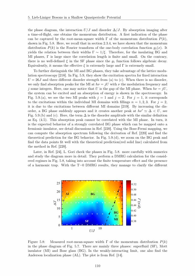
5. Lieb-Liniger Bosons in a Shallow Quasiperiodic Potential
the phase diagram, the interaction U/J and disorder ∆/J . By absorption imaging aftera time-of-flight, one obtains the momentum distribution. A first indication of the phasecan be captured by the root-mean-square width Γ of the momentum distribution P (k),shown in Fig. 5.8. Here, we recall that in section 2.3.4, we have shown that the momentumdistribution P (k) is the Fourier transform of the one-body correlation function g1(x). Ityields the relation between their widths Γ ∼ 1/ξ. Therefore, for the insulating BG andMI phases, Γ is large since the correlation length is finite and small. On the contrary,there is no well-defined ξ in the SF phase since the g1 function follows algebraic decay.Equivalently, it means the effective ξ is extremely large and Γ is extremely small.
To further distinguish the MI and BG phases, they take advantage of the lattice modu-lation spectroscopy [218]. In Fig. 5.9, they show the excitation spectra for fixed interactionU = 26J and three different disorder strength from (a) to (c). When there is no disorder,we only find absorption peaks for the MI at hν = jU with ν the modulation frequency andj some integers. Here, one may notice that U is the gap of the MI phase. When hν = jU ,the system can be excited and an absorption of energy is shown in the spectroscopy. InFig. 5.9.(a), we see the two MI peaks with j = 1 and j = 2. For j = 1, it correspondsto the excitations within the individual MI domains with fillings n = 1, 2, 3. For j = 2,it is due to the excitations between different MI domains [219]. By increasing the dis-order, a BG phase suddenly appears and it creates another peak at hν ′ ' ∆ < U , seeFig. 5.9.(b) and (c). Here, the term ∆ is the disorder amplitude with the similar definitionas Eq. (4.5). This absorption peak cannot be correlated with the MI phase. In turn, itis the expected behavior of a strongly correlated BG phase which can be mapped onto afermionic insulator, see detail discussions in Ref. [220]. Using the Bose-Fermi mapping, wecan compute the absorption spectrum following the derivation of Ref. [220] and find thetheoretical prediction for the BG behavior. In Fig. 5.9.(d), we zoom on the BG peak andfind the data points fit well with the theoretical prediction(red solid line) calculated fromthe method in Ref. [220].
Later, in Ref. [24], L. Gori check the phases in Fig. 5.8. more carefully with numericsand study the diagram more in detail. They perform a DMRG calculation for the consid-ered regimes in Fig. 5.8, taking into account the finite temperature effect and the presenceof a harmonic trap. With the T=0 DMRG results, they manage to clarify the different
Figure 5.8: Measured root-mean-square width Γ of the momentum distribution P (k)in the phase diagram of Fig. 5.7. There are mainly three phases: superfluid (SF), Mottinsulator (MI) and Bose glass (BG). In the weakly-interacting limit, one also find theAnderson localization phase (AL). The plot is from Ref. [14].
110

5. Lieb-Liniger Bosons in a Shallow Quasiperiodic Potential
Figure 5.9: Excitation spectrum for three points of the phase diagram: the interactionstrength U = 26J and disorder (a). ∆ = 0J . (b). ∆ = 6.5J . (c). ∆ = 9.5J . The plot isfrom Ref. [14].
expected phases in Fig. 5.8, noted by the texted phase name. Along the zero interactionU = 0 line, one find the transition from SF phase to Anderson localization by increasing∆. On the other limit ∆ = 0, we see the SF to MI transition by increasing the interactionU . For a fixed and not so strong interaction, one always finds the SF-BG transition byincreasing ∆. Finally, at low disorder and strong interactions, one find a mixture of MIand BG phase, thanks to the presence of the harmonic trap.
Beyond the zero-temperature calculations, L. Gori et al perform further the finite-Tphenomenological approaches based on T = 0DMRG calculations of the momentum dis-tribution P (k), see Fig. 5.10. For the aspect of the temperature effect, they calculatefirst T = 0 DMRG results of P (k) and get its Fourrier transform, i.e. the one-body cor-relation length gi,j(T ) at the distance |i − j| and temperature T . Then, they propose aphenomenological ansatz where they introduce the modified correlations
gi,j(T ) = Ce−|i−j|/ξTgi,j(T = 0) (5.10)
with gi,j(T ) the finite temperature correlation function, ξT the effective thermal correlationlength and C the normalization factor. Fitting the experimental data with Eq. (5.10), onecan get the information for the thermal effect on the correlation length. Four typicalexamples of the momentum distribution P (k) are shown as the small subplots on the leftand right sides. The different curves are the zero-T DMRG results (black solid lines),
Figure 5.10: The U − ∆ diagram for the momentum width Γ from finite-T DMRGcalculations. The detailed plots of the momentum distribution P (k) are shown for fourtypical points. The different curves are the zero-T DMRG results (black solid lines),experimental data (blue dash-dotted lines) and fit of finite-T phenomenological ansatz(reddashed lines). The plot is from Ref. [24].
111

5. Lieb-Liniger Bosons in a Shallow Quasiperiodic Potential
finite-T phenomenological fit (red dashed lines) and experimental data (blue dash-dottedlines). Although the finite temperature results are similar as the zero-temperature casefor the two points in the strongly-interacting regime, there is clearly a thermal broadeningfor the correlation length in the intermediate interaction regime. These results suggestthat the measurements are strongly altered by the finite temperature effects. Therefore,in the next section, we will study the Bose glass phase transition in shallow quasiperiodicpotentials, where the temperature effect is significantly reduced.
5.2 The phase diagram for the shallow quasiperiodic systems
Now, we turn to full continuous study of the phase diagram for shallow quasiperiodicsystems. Instead of the deep lattice limit, now we turn to the shallow lattice case, i.e. wecome back to the Hamiltonian Eq. (5.9). In particular, we are interested in the regime wherethe quasiperiodic potential is on the same scale of the recoil energy Er and is bichromaticwith equal amplitudes, i.e.
V (x) =V
2
[cos (2k1x) + cos (2k2x+ ϕ)
]. (5.11)
where the spatial frequencies k1 and k2 are incommensurate. In the following calculations,we will use the spatial period of the first lattice, a = π/k1, and the corresponding recoilenergy, Er = ~2k2
1/2m, as the space and energy units, respectively.We firstly start with the single-particle problem, i.e. g = 0 for Eq. (5.9). In Chapter 4,
we have studied in detail the single-particle problem for the case r = k2/k1 = (√
5− 1)/2.As shown in Ref. [176], both the critical potential Vc and mobility edge Ec strongly dependon the incommensurate ratio r. In this chapter, we use the incommensurate ratio close tothe experimental value of Refs. [14,24], it yields
r =λ1
λ2=
856nm1064nm
' 67
83' 0.807. (5.12)
Thus, we repeat the similar calculation for single-particle problem with a different valueof r = 0.807 to provide a basis for the further study in this chapter.
Here, we recall that the main procedure is to determine the single-particle eigenstatesby using exact diagonalization and computing the inverse participation ratio (IPR),
IPRn =
∫dx |Ψn(x)|4(∫dx |Ψn(x)|2
)2 , (5.13)
Figure 5.11: Critical potential and mobility edge for the single-particle problem in theshallow bichromatic lattice with r ' 0.807. (a) Ground-state IPR versus the quasiperiodicamplitude V for various system sizes. Darker lines correspond to increasing system sizes,L/a = 50 (light blue), 200 (blue), 500 (dark blue), and 1000 (black). (b) Rescaled IPR ofthe ground state, IPR0 ×
√La using the same data as in panel (a). (c) Scaling exponent
τ of the IPR as a function of eigenenergy E for the quasiperiodic amplitude V = 1.5Er. Itis computed for a system size varying from L/a = 200 to 2000.
112
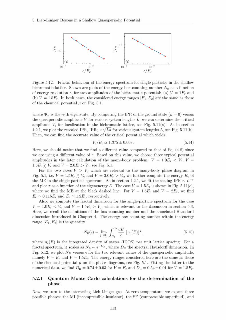
5. Lieb-Liniger Bosons in a Shallow Quasiperiodic Potential
Figure 5.12: Fractal behaviour of the energy spectrum for single particles in the shallowbichromatic lattice. Shown are plots of the energy-box counting number NB as a functionof energy resolution ε, for two amplitudes of the bichromatic potential: (a) V = 1Er and(b) V = 1.5Er. In both cases, the considered energy ranges [E1, E2] are the same as thoseof the chemical potential µ on Fig. 5.1.
where Ψn is the n-th eigenstate. By computing the IPR of the ground state (n = 0) versusthe quasiperiodic amplitude V for various system lengths L, we can determine the criticalamplitude Vc for localization in the bichromatic lattice, see Fig. 5.11(a). As in section4.2.1, we plot the rescaled IPR, IPR0×
√La for various system lengths L, see Fig. 5.11(b).
Then, we can find the accurate value of the critical potential which yields
Vc/Er ' 1.375± 0.008. (5.14)
Here, we should notice that we find a different value compared to that of Eq. (4.8) sincewe are using a different value of r. Based on this value, we choose three typical potentialamplitudes in the later calculation of the many-body problem: V = 1.0Er < Vc, V =1.5Er & Vc and V = 2.0Er > Vc, see Fig. 5.1.
For the two cases V > Vc which are relevant to the many-body phase diagram inFig. 5.1, i.e. V = 1.5Er & Vc and V = 2.0Er > Vc, we further compute the energy Ec ofthe ME in the single-particle spectrum. As in section 4.2.1, we fit the scaling IPR ∼ L−τ
and plot τ as a function of the eigenenergy E. The case V = 1.5Er is shown in Fig. 5.11(c),where we find the ME at the black dashed line. For V = 1.5Er and V = 2Er, we findEc ' 0.115Er and Ec ' 1.2Er, respectively.
Also, we compute the fractal dimension for the single-particle spectrum for the caseV = 1.0Er < Vc and V = 1.5Er > Vc, which is relevant to the discussion in section 5.3.Here, we recall the definitions of the box counting number and the associated Hausdorffdimension introduced in Chapter 4. The energy-box counting number within the energyrange [E1, E2] is the quantity
NB(ε) = limq→0+
∫ E2
E1
dE
ε
[nε(E)
]q, (5.15)
where nε(E) is the integrated density of states (IDOS) per unit lattice spacing. For afractal spectrum, it scales as NB ∼ ε−DH , where DH the spectral Hausdorff dimension. InFig. 5.12, we plot NB versus ε for the two relevant values of the quasiperiodic amplitude,namely V = Er and V = 1.5Er. The energy ranges considered here are the same as thoseof the chemical potential µ on the phase diagrams, see Fig. 5.1. Fitting the latter to thenumerical data, we find DH = 0.74± 0.03 for V = Er and DH = 0.54± 0.01 for V = 1.5Er.
5.2.1 Quantum Monte Carlo calculations for the determination of thephase
Now, we turn to the interacting Lieb-Liniger gas. At zero temperature, we expect threepossible phases: the MI (incompressible insulator), the SF (compressible superfluid), and
113

5. Lieb-Liniger Bosons in a Shallow Quasiperiodic Potential
the BG (compressible insulator). They can be identified through the values of only twoquantities, namely the compressibility κ and the superfluid fraction fs. Accurate valuesof both are found using large-scale, path-integral quantum Monte Carlo (QMC) calcula-tions in continuous space using the worm algorithm implementation [58,59] as introducedin Chapter 2. The calculation is performed within the grand-canonical ensemble at thechemical potential µ and the temperature T . We span a large number of boson configu-rations within both the physical Z-sector (closed worldlines) and the unphysical G-sector(worms, i.e. worldlines with open ends). The average number of particles N is found fromthe statistics of worldlines within the Z-sector. It yields the particle density ρ = N/L,where L is the system size, and the compressibility κ = ∂ρ/∂µ. One can find details inthe section 2.3.1. For the superfluid fraction fs = Υs/ρ, it can be found from the thesuperfluid stiffness Υs using the winding number estimator, as introduced in section 2.3.2.The calculation of these three quantities allows us to discriminate the 3 phases at zerotemperature and most of them at finite temperature except BG and NF.
For distinguishing the BG and NF phases at finite temperature, we need to further cal-culate the one-body correlation function g1(x) at different temperatures. While ξ remainsunchanged versus temperature for BG phase, it strongly depends on T for the thermalNF phase. Detailed discussion on this point can be found in section 5.3.1. We recall thedefinition of the one-body correlation function,
g1(x) =
∫dx′
L〈Ψ(x′ + x)†Ψ(x′)〉, (5.16)
where Ψ(x) is the Bose field operator. In the QMC calculations, it is computed from thestatistics of worms with open ends at x′ and x′ + x within the G-sector, see section 2.3.4for details. For insulating phases (i.e. MI, BG and NF phases), it behaves as
g1(x) ∼ exp
(−|x|ξ
)(5.17)
where ξ is the correlation length. Fitting the function g1(x) ∼ exp (−|x|/ξ) and obtainingthe parameter ξ, we can distinguish the BG from NF regimes via the temperature depen-dence (see details in Section 5.3.1). To make a short conclusion, the detailed properties ofeach phase can be found in Table 5.2.
Phase SF fraction fs Compressibility κ T -dep. of corr. length ∂ξ/∂TSuperfluid (SF) 6= 0 6= 0 /
Mott-insulator (MI) = 0 = 0 ∼ 0
Bose-glass (BG) = 0 6= 0 ∼ 0
Normal fluid (NF) = 0 6= 0 6= 0
Table 5.2: Identification of the (zero-temperature) quantum phases and finite-temperatureregimes from quantum Monte Carlo calculations. Note that the one-body correlationfunction g1(x) is algebraic in the superfluid regime and the correlation length ξ(T ) is notdefined.
Figure 5.13 shows typical results for the particle density ρ, the compressibility κ, andthe superfluid fraction fs. The six panels correspond to cuts of the six diagrams of Fig. 5.1at the interaction strength −a1D/a = 0.1.
Figure 5.13(a1): We consider first the case V = Er,i.e. below the critical potential and zerotemperature T = 0. In this case, we find an alternation of compressible (κ > 0) and in-compressible (κ = 0) phases, in exact correspondance with superfluidity: the compressiblephases always have a finite superfluid fraction (fs > 0) while the incompressible phases are
114

5. Lieb-Liniger Bosons in a Shallow Quasiperiodic Potential
Figure 5.13: Typical QMC results for the density ρ, the superfluid fraction fs, and thecompressibility κ as a function of the chemical potential µ. The various panels are cutsof the diagrams of Fig. 5.1 at the interaction strength −a1D/a = 0.1: (a1) V = Er andkBT/Er = 0.001, (a2) V = 1.5Er and kBT/Er = 0.002 (a3) V = 2Er and kBT/Er = 0.002,(b1)-(b3) Same as in panle (a) but at temperature kBT/Er = 0.015.
always non-superfluid (fs = 0). They correspond to SF (red areas) and MI phases (blueareas), respectively. There is no BG phase existed which is consistent with the fact thatthe potential amplitude is below the critical potential, V < Vc ' 1.38Er.
Figure 5.13(a2): We consider then the case V = 1.5Er,i.e. slightly above the criticalpotential, and zero temperature T = 0. Here we find a similar behaviour for large enoughchemical potential, µ & 0.1Er. For smaller chemical potentials, however, we find clearsignatures of BG phases, corresponding to a compressible insulator (κ > 0 and fs = 0,yellow areas). Here, the BG phases are separated by MI phases (κ = 0 and fs = 0,blue areas). As expected, in the strongly-interacting limit, the BG phase appears only forµ < Ec ' 0.115Er, i.e. the single-particle mobility edge in Fig. 5.11.(c) (dashed black line).
Figure 5.13(a3) [V = 2Er even more above the critical potential; T = 0]: We considerthen the case V = 2.0Er,i.e. even more above the critical potential, and zero temperatureT = 0. In this case, the Bose gas is non-superfluid, fs = 0, in the whole range of thechemical potential considered here. It, however, shows an alternance of compressible andincompressible phases, corresponding to BG (yellow areas) and MI (blue areas) phases,respectively. Note that for V = 2Er the single-particle mobility edge is Ec ' 1.2Er, whichis beyond the considered range of the chemical potential.
Figure 5.13(b1-b3): Finally, we consider the case of finite temperature T = 0.015Er. Thelower panel shows the finite-temperature counterpart of the upper panel. The variousregimes are characterized by the same criteria as for zero temperature. First, we findregimes with vanishingly small compressibility and superfluid fraction. They correspondto regimes where the zero-temperature MI is unaffected by the finite temperature effects(blue areas, all panels). Second, although superfluidity is absent in the thermodynamiclimit, we find compressible regimes with a clear non-zero superfluid fraction in our systemof size L = 83a for weak enough quasiperiodic potential (red areas, left panel). We referto such regimes as finite-size superfluids. We have checked that the one-body correlation
115

5. Lieb-Liniger Bosons in a Shallow Quasiperiodic Potential
function is, consistently, algebraic over the full system size in these regimes (see below).Third, we find insulating, compressible regimes (fs = 0 and κ > 0). At finite temperature,however, the values of fs and κ are not sufficient to distinguish the BG and NF phases,which are thus discriminated via the temperature dependence of the correlation lengthξ(T ): the absence of temperature dependence shows that the quantum phase is unaffectedby the thermal fluctuations and the corresponding regimes are identified as the BG (yellowareas). Conversely, the regimes where the correlation length shows a sizable temperaturedependence are identified as the NF (light blue areas).
5.2.2 Analysis of the phase diagram
Now, we come back to the results of the whole phase diagram. With the method mentionedabove, we are able to identify the different phases of the system at varying interactions,chemical potentials, potential amplitudes and temperatures. The computed phase diagramis our main result of this chapter and plotted in Fig. 5.1. The upper row on Fig. 5.1 showsthe quantum phase diagrams versus the inverse interaction strength and the chemicalpotential, for increasing amplitudes of the quasiperiodic potential. They are found fromQMC calculations of κ and fs at a vanishingly small temperature. In practice, we have usedkBT ∼ 0.001 − 0.002Er, where kB is the Boltzmann constant, and we have checked thatthere is no sizable temperature dependence at a lower temperature. The results thus fairlyaccount for the zero-temperature phase diagram of the system. For V < Vc, no localizationis expected and we only find SF and MI phases, see panel (a1). The SF dominates at largechemical potentials and weak interactions. Strong enough interactions destabilize the SFphase and Mott lobes open, with fractional occupation numbers (ρa = r, 2r − 1, 2 − 2r,1 − r from top to bottom). The number of lobes increases with the interaction strengthand eventually become dense in the hard-core limit (see below). For V > Vc and a finiteinteraction, a BG phase , reminiscent of single-particle localization, develops in betweenthe MI lobes up to the single-particle ME at µ = Ec, see panel (a2). There, the SF fractionis strictly zero and the compressibility has a sizable, non-zero value, within QMC accuracy.When the quasiperiodic amplitude V increases, the BG phase extends at the expense ofboth the MI and SF phases, see panel (a3).
The lower row on Fig. 5.1 shows the counterpart of the previous diagrams at the fi-nite temperature T = 0.015Er/kB, corresponding to the minimal temperature in Ref. [12].While quantum phases may be destroyed by arbitrarily small thermal fluctuations, thefinite-size systems we consider (L = 83a) retain characteristic properties, reminiscent ofthe zero-temperature phases. The SF, MI, and BG regimes shown on Figs. 5.1(b1)-(b3)are identified accordingly. While the former two are easily identified, special care shouldbe taken for the BG, which cannot be distinguished from the normal fluid (NF), sinceboth are compressible insulators (κ > 0 and fs = 0). A key difference, however, is thatcorrelations are suppressed by the disorder in the BG and by thermal fluctuations in theNF. To identify the BG regime, we thus further require that the suppression of correla-tions is dominated by the disorder, i.e. the correlation length is nearly independent of thetemperature. The QMC results show that the NF develops at low density and strong in-teractions, see panel (b1). For a moderate quasiperiodic amplitude, it takes over the BG,which is completely destroyed, see panel (b2). For a strong enough quasiperiodic potential,however, the BG is robust against thermal fluctuations and competes favourably with theNF regime, see panel (b3). We hence find a sizable BG regime, which should thus beobservable at temperatures accessible to current experiments using 1D quantum gases.
116
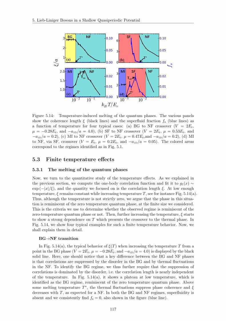
5. Lieb-Liniger Bosons in a Shallow Quasiperiodic Potential
Figure 5.14: Temperature-induced melting of the quantum phases. The various panelsshow the coherence length ξ (black lines) and the superfluid fraction fs (blue lines) asa function of temperature for four typical cases: (a) BG to NF crossover (V = 2Er,µ = −0.28Er, and −a1D/a = 4.0), (b) SF to NF crossover (V = 2Er, µ = 0.53Er, and−a1D/a = 0.2), (c) MI to NF crossover (V = 2Er, µ = 0.47Er,and −a1D/a = 0.2), (d) MIto NF, via SF, crossover (V = Er, µ = 0.2Er, and −a1D/a = 0.05). The colored areascorrespond to the regimes identified as in Fig. 5.1.
5.3 Finite temperature effects
5.3.1 The melting of the quantum phases
Now, we turn to the quantitative study of the temperature effects. As we explained inthe previous section, we compute the one-body correlation function and fit it to g1(x) ∼exp (−|x|/ξ), and the quantity we focused on is the correlation length ξ. At low enoughtemperature, ξ remains constant while increasing temperature T , see for instance Fig. 5.14(a).Thus, although the temperature is not strictly zero, we argue that the phase in this situa-tion is reminiscent of the zero temperature quantum phase, at the finite size we considered.This is the criteria we use to determine whether the observed regime is reminiscent of thezero-temperature quantum phase or not. Then, further increasing the temperature, ξ startsto show a strong dependence on T which presents the crossover to the thermal phase. InFig. 5.14, we show four typical examples for such a finite temperature behavior. Now, weshall explain them in detail.
BG→NF transition
In Fig. 5.14(a), the typical behavior of ξ(T ) when increasing the temperature T from apoint in the BG phase (V = 2Er, µ = −0.28Er, and −a1D/a = 4.0) is displayed by the blacksolid line. Here, one should notice that a key difference between the BG and NF phasesis that correlations are suppressed by the disorder in the BG and by thermal fluctuationsin the NF. To identify the BG regime, we thus further require that the suppression ofcorrelations is dominated by the disorder, i.e. the correlation length is nearly independentof the temperature. In Fig. 5.14(a), it shows a plateau at low temperature, which isidentified as the BG regime, reminiscent of the zero temperature quantum phase. Abovesome melting temperature T ∗, the thermal fluctuations suppress phase coherence and ξdecreases with T , as expected for a NF. In both the BG and NF regimes, superfluidity isabsent and we consistently find fs = 0, also shown in the figure (blue line).
117

5. Lieb-Liniger Bosons in a Shallow Quasiperiodic Potential
Figure 5.15: One-body correlation function g1(x) for the parameters V = 2Er, µ =−0.28Er, and −a1D/a = 4.0. The calculations are for two different temperatures: (a) T =0.004Er/kB (BG regime) and (b) T = 0.04Er/kB (NF regime). The upper and lowerpanels show plots of the same data in semi-log and log-log scales, respectively. The dashedred lines indicate linear fits to g1(x) in semi-log scale. It yields the coherence lengths(a) ξ ' 2.86a and (b) ξ = 1.81a, respectively.
In Fig. 5.15, we show in detail the behaviour of g1(x) for a typical point of BG andNF in Fig. 5.14(a) respectively. The upper and lower panels show plots of the same datain semi-log and log-log scales, respectively. We find, in both cases, that g1(x) is betterfitted by an exponential function, g1(x) ∼ exp(−|x|/ξ), rather than an algebraic function.This is consistent with the expected behaviour in insulating regimes. Fitting the linearslope in semi-log scale (dotted red line), we extract the correlation length ξ(T ). Here,the case in subplot (a) has the correlation length ξ/a = 2.86, which is the same valueof the zero-temperature limit ξ0. Thus, we identify it as finite temperature BG phase inthe reminiscent of the zero temperature quantum phase. On the contrary. for the case insubplot (b), we find ξ = 1.81a < ξ0, where a strong finite-temperature is observed. Weconclude the system is in NF phase in this case.
SF→NF transition
Consider now increasing the temperature from a point in the SF phase at T = 0, seeFig. 5.14(b). For low enough T , we find a finite SF fraction fs, which, however, stronglydecreases with T . In this regime, the correlation function shows a characteristic algebraicdecay over the full system of length L = 83a. The sharp decrease of fs allows us to identifya rather well defined temperature T ∗ beyond which we find a NF regime, characterizedby a vanishingly small fs. In this regime, the correlation function consistently shows anexponential decay and the correlation length ξ(T ) decreases with T . This scenario isconsistent with the expected suppression of coherence induced by thermal fluctuations.
In Fig. 5.16, we show examples of correlation functions for two typical points in theSF and NF regimes of Fig. 5.14(b). On the one hand, the left panel corresponds to thetemperature T = 2.4 × 10⁻³Er/kB, where we find a finite-size SF. Consistently, the one-body correlation function is well fitted by an algebraic function (dotted red line), butnot by an exponential function, over the full system size. On the other hand, the rightpanel corresponds to the temperature T = 3 × 10⁻²Er/kB, where we find a compressibleinsulator with a temperature-dependent correlation length. Consistently, the one-bodycorrelation function is here better fitted by an exponential function (dotted red line) thanby an algebraic function, over the full system size.
118

5. Lieb-Liniger Bosons in a Shallow Quasiperiodic Potential
Figure 5.16: One-body correlation function g1(x) for the parameters V = 2Er, µ = 0.53Er,and −a1D/a = 0.2. The calculations are for two different temperatures: (a) T = 2.4 ×10⁻³Er/kB (finite-size SF regime) and (b) T = 0.03Er/kB (NF regime). The upper andlower panels show plots of the same data in semi-log and log-log scales, respectively. Thedashed red lines indicate linear fits to g1(x) in semi-log scale or log-log scale.
MI→NF transition
Consider now increasing the temperature from a point in a MI lobe at T = 0, a typicalexample is shown on Figs. 5.14(c). As expected, below a melting temperature T ∗, thecorrelation length shows a plateau, identified as the MI regime. Quite counterintuitively,however, we find that above T ∗ the phase coherence is enhanced by thermal fluctuations, upto some temperature Tm, beyond which it is finally suppressed. This anomalous behavior issignaled by the nonmonotony of the correlation length ξ(T ), see Fig. 5.14(c). We interpretthis behavior from the competition of two effects. On the one hand, a finite but smalltemperature permits the formation of particle-hole pair excitations, which are extended andsupport phase coherence. This effect, which is often negligible in strong lattices, is enhancedin shallow lattices owing to the smallness of the Mott gaps, particularly in the quasiperiodiclattice where Mott lobes with fractional fillings appear [86,192]. This favours the onset ofa finite-range coherence at finite temperature. On the other hand, when the temperatureincreases, a larger number of extended pairs, which are mutually incoherent, is created.This suppresses phase coherence on a smaller and smaller length scale, hence competingwith the former process and leading to the nonmonotonic temperature dependence of thecoherence length.
MI→SF→NF transition
In Fig. 5.14(d), we show the melting effect for another point which is MI at zerotemperature and inside a MI lobe surrounded by a SF phase. In this case, the nonmonotonictemperature effect on the correlation length still exists. It is even strong enough to inducea finite superfluid fraction fs, and correspondingly an algebraic correlation function in ourfinite-size system, see Fig. 5.14(d).
To further confirm the appearance of the SF region in this case, Fig. 5.17 shows theg1(x) functions, in both semi-log (upper panel) and log-log (lower panel) scales, for theparameters of Fig. 5.14(d) and three different temperatures: (a) T = 8 × 10⁻⁴Er/kB,corresponding to the MI regime, (b) T = 4 × 10⁻³Er/kB, corresponding to the finite-sizeSF regime, and (c) T = 3× 10⁻²Er/kB, corresponding to the NF regime [see Fig. 5.14(d)].Consistently, we find that g1(x) is better fitted by an exponential function in the insulatingregimes [MI and NF, panels (a) and (c)] and by an algebraic function in the finite-size SF
119

5. Lieb-Liniger Bosons in a Shallow Quasiperiodic Potential
Figure 5.17: One-body correlation function g1(x) for the parameters V = Er, µ = 0.2Er,and −a1D/a = 0.05 at three different temperatures: (a) T = 8 × 10⁻⁴Er/kB (MI regime),(b) T = 4 × 10⁻³Er/kB (finite-size SF regime), and (c) T = 3 × 10⁻²Er/kB (NF regime).The upper and lower panels show plots of the same data in semi-log and log-log scales,respectively. The dashed red lines indicate linear fits to g1(x) in semi-log or log-log scale.
regime [panel (b)]. This is further confirmed by the calculation of the Pearson correlationcoefficients P for a linear fit of g1(x) in semi-log and log-log scales, see Fig. 5.18. ThePearson correlation coefficient P for a linear fit of data (X,Y ) defines as
P (X,Y ) =cov(X,Y )
σXσY(5.18)
with cov(X,Y ) the covariance of (X,Y ) and σX is the variance of X. The closer P is tounity, the better the linear fit. Figure 5.18 confirms that the correlation function is closerto an exponential function in the MI (dark blue) and NF (light blue) regimes, and closerto an algebraic function in the superfluid regime (red).
Bose glass at higher temperatures in actual experiment
Results such as those shown on Fig. 5.14(a) provide us with the condition of experi-mental temperature for observing the BG phase. Here, we discuss further the observabilityin actual experiment based on our phase diagram. In the Fig 5.1, the diagrams of the
Figure 5.18: Pearson’s correlation coefficient for linear fits of one-body correlation functiong1(x) for the parameters V = Er, µ = 0.2Er, and −a1D/a = 0.05, in semi-log scale (solidblue line) and log-log scale (solid green line). The shaded areas correspond to the MI (darkblue), SF (red), and NF (light blue) regimes, determined as in Fig. 2(d).
120

5. Lieb-Liniger Bosons in a Shallow Quasiperiodic Potential
Figure 5.19: Existence of the BG regime for V = 2Er at higher temperatures. (a) Re-production of the Fig. 5.1(b3), indicating the MI (blue), SF (red), BG (yellow), andNF (green) regimes at the temperature T = 0.05Er/kB. The markers indicate pointswhere the melting temperature T ∗ of the BG phase is kBT ∗/Er < 0.05 (black squares),0.05 < kBT
∗/Er < 0.1 (blue disks) or kBT ∗/Er > 0.1 (red disks). (b) Temperature depen-dence of the correlation length ξ for the four points indicated on panel (a). The dashed blueand red lines indicate the temperatures T = 0.05Er/kB and T = 0.1Er/kB, respectively.The background colors indicate the BG (yellow) and NF (light blue) regimes.
lower row are computed at the finite temperature T = 0.015Er/kB. It corresponds tothe temperature T = 1.5nK for 1D 133Cs atoms, corresponding approximately to the low-est temperatures reported in Ref. [12]. For the amplitude of the quasiperiodic potentialV = 2Er, its shows a sizable BG regime, see red disks in Fig. 5.19(a), which reproducesthe Fig. 5.1(b3). The BG should be observable in such an experiment.
Moreover, we have checked that a sizable BG regime survives up to higher temper-atures. For instance the experiment of Ref. [12] reported temperatures in the range1nK. T . 10nK for 133Cs atoms, corresponding to 0.01 . kBT/Er . 0.1. The experimentof Ref. [14] was operated at T ' 15nK for 39K atoms, corresponding to kBT/Er ' 0.07.We have studied the temperature dependence of the correlation length ξ as determinedfrom exponential fits to the one-body correlation function g1(x). Some examples areshown on Fig. 5.14 as well as in Figs. 5.19(b1)-(b4). The melting temperature T ∗ ofthe BG is the temperature where ξ(T ) starts to decrease. The points in the BG regimewe have check are indicated by markers on Fig. 5.19(a): black squares correspond tocases where kBT ∗/Er < 0.05 [see for instance Fig.5.19(b4)], blue disks to cases where0.05 < kBT
∗/Er < 0.1 [see for instance Fig. 5.19(b3)], and red disks to cases wherekBT
∗/Er > 0.1 [see for instance Fig. 5.19(b1) and (b2)]. It shows that sizable BG regimesare still found at T ' 0.05Er/kB and at T ' 0.1Er/kB, and should thus be observable inexperiments such as those of Refs. [12,14].
5.3.2 Fractal Mott lobes
According to the statement in Ref. [221], the typical scale of the melting temperature forthe Mott lobe is given by
T ∗ ∝ ∆/kB (5.19)
where ∆ is the width of the lobe. More precisely, it normally appears typically at thetemperature scale T ∼ 0.1∆/kB. In the quasiperiodic lattice, however, there is no typicalgap, owing to the fractal structure of the Mott lobes, inherited from that of the single-particle spectrum, see discussions in section 4.3 and Refs. [23, 86, 192]. In this subsection,
121

5. Lieb-Liniger Bosons in a Shallow Quasiperiodic Potential
Figure 5.20: Equation of state ρ(µ) for free fermions, equivalent to hard-core bosons.(a) Same as Fig. 5.1(a2), V = 1.5Er, r = 0.807, T = 2× 10⁻³Er/kB. (b) and (c) are sameas panel (a) but with smaller temperatures, T = 8× 10⁻⁴Er/kB and T = 1.6× 10⁻⁴Er/kBcorrespondingly.
we will study in detail the finite temperature effect for the fractal Mott lobes and its linkwith the fractality of the energy spectrum.
Smoothing of the spectral gaps in the hard-core limit
First of all, we want to understand better the origin of the fractal Mott lobes. Westart with the equation of state which is linked with the fractality of the single-particlespectrum. As discussed before, Bose-Fermi mapping in the hard-core limit allows us towrite the equation of state
ρ(µ) ' 1
L
∑j
fFD(Ej − µ) (5.20)
with the Fermi-Dirac distribution
fFD(E) =1
eE/kBT + 1, (5.21)
where Ej is the energy of the j-th eigenstate of the single-particle Hamiltonian. At zerotemperature, fFD(E) is simply a Heaviside step function centred at E = µ. Thus, it simplyfills all the state below µ with one particle per state and leaves empty the states above µ.Therefore, with the single-particle energy spectrum, one can recover the equation of statein the hard-core limit. Owing to the fractality of the single-particle spectrum (see detailsin Sec. 4.3), at strictly zero temperature, ρ(µ) is a discontinuous step-like function at anyscale.
Any finite temperature T smoothes out all the gaps smaller than the typical energy scalekBT . For instance, Fig. 5.20(a) reproduces the equation of state plotted on the left-handside of the Fig. 5.1(a2), corresponding to the temperature T = 2 × 10⁻³Er/kB. One seescompressible regions between the plateaus. When the temperature decreases, however, newplateaus appear within these compressible regions. See for instance Fig. 5.20(b) and (c),which correspond to the temperatures T = 8× 10⁻⁴Er/kB and T = 1.6× 10⁻⁴Er/kB. Thisis consistent with the pure step-like equation of state expected at strictly zero temperature.The new plateaus observed on Fig. 5.20(b) and (c) correspond to Mott gaps for interactingbosons. By taking a smaller value of T and larger values of g, we shall see these smallergaps. They, however, appear at a stronger interaction strength than that considered inthis study. They are thus irrelevant to our discussion.
The compressible fraction and spectrum fractal dimension
To get further insight into the description of the melting of the MI lobes, consider thecompressible phase fraction, i.e. the complementary of the fraction of MI lobes,
K = limq→0+
∫ µ2
µ1
dµ
µ2 − µ1
[κ(µ)
]q, (5.22)
122
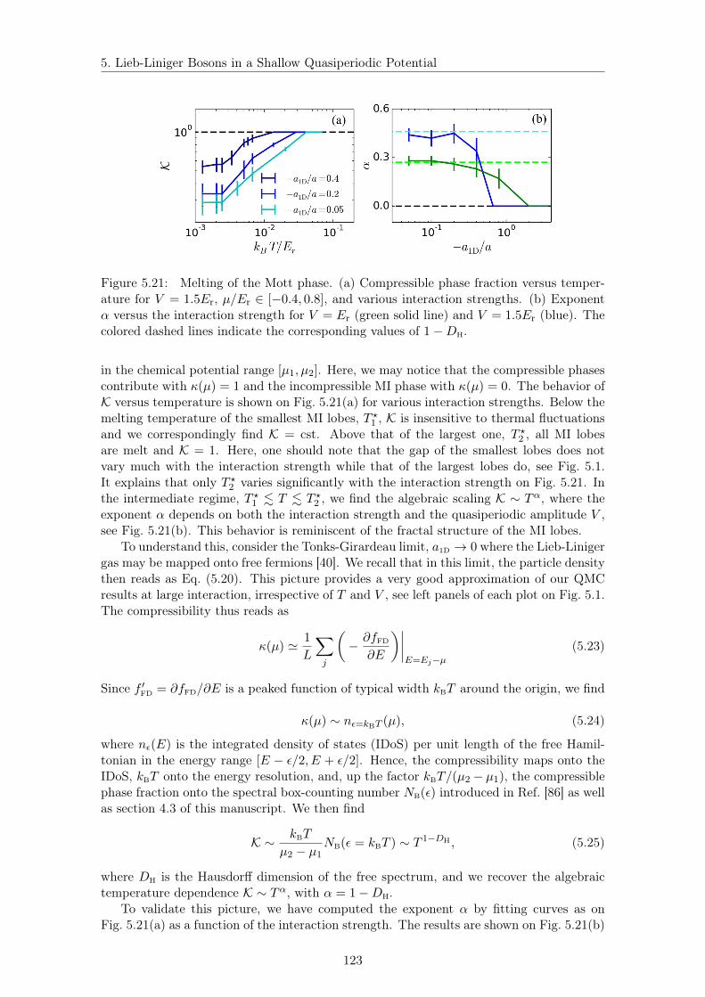
5. Lieb-Liniger Bosons in a Shallow Quasiperiodic Potential
Figure 5.21: Melting of the Mott phase. (a) Compressible phase fraction versus temper-ature for V = 1.5Er, µ/Er ∈ [−0.4, 0.8], and various interaction strengths. (b) Exponentα versus the interaction strength for V = Er (green solid line) and V = 1.5Er (blue). Thecolored dashed lines indicate the corresponding values of 1−DH.
in the chemical potential range [µ1, µ2]. Here, we may notice that the compressible phasescontribute with κ(µ) = 1 and the incompressible MI phase with κ(µ) = 0. The behavior ofK versus temperature is shown on Fig. 5.21(a) for various interaction strengths. Below themelting temperature of the smallest MI lobes, T ?1 , K is insensitive to thermal fluctuationsand we correspondingly find K = cst. Above that of the largest one, T ?2 , all MI lobesare melt and K = 1. Here, one should note that the gap of the smallest lobes does notvary much with the interaction strength while that of the largest lobes do, see Fig. 5.1.It explains that only T ?2 varies significantly with the interaction strength on Fig. 5.21. Inthe intermediate regime, T ?1 . T . T ?2 , we find the algebraic scaling K ∼ Tα, where theexponent α depends on both the interaction strength and the quasiperiodic amplitude V ,see Fig. 5.21(b). This behavior is reminiscent of the fractal structure of the MI lobes.
To understand this, consider the Tonks-Girardeau limit, a1D → 0 where the Lieb-Linigergas may be mapped onto free fermions [40]. We recall that in this limit, the particle densitythen reads as Eq. (5.20). This picture provides a very good approximation of our QMCresults at large interaction, irrespective of T and V , see left panels of each plot on Fig. 5.1.The compressibility thus reads as
κ(µ) ' 1
L
∑j
(− ∂fFD
∂E
)∣∣∣∣E=Ej−µ
(5.23)
Since f ′FD = ∂fFD/∂E is a peaked function of typical width kBT around the origin, we find
κ(µ) ∼ nε=kBT (µ), (5.24)
where nε(E) is the integrated density of states (IDoS) per unit length of the free Hamil-tonian in the energy range [E − ε/2, E + ε/2]. Hence, the compressibility maps onto theIDoS, kBT onto the energy resolution, and, up the factor kBT/(µ2 − µ1), the compressiblephase fraction onto the spectral box-counting number NB(ε) introduced in Ref. [86] as wellas section 4.3 of this manuscript. We then find
K ∼ kBT
µ2 − µ1NB(ε = kBT ) ∼ T 1−DH , (5.25)
where DH is the Hausdorff dimension of the free spectrum, and we recover the algebraictemperature dependence K ∼ Tα, with α = 1−DH.
To validate this picture, we have computed the exponent α by fitting curves as onFig. 5.21(a) as a function of the interaction strength. The results are shown on Fig. 5.21(b)
123

5. Lieb-Liniger Bosons in a Shallow Quasiperiodic Potential
for two values of the quasiperiodic amplitude (colored solid lines). As expected, we findα → 1 − DH (colored dashed lines) in the Tonks-Girardeau limit, a1D → 0. When theinteraction strength decreases, the fermionization picture breaks down. The exponent αthen decreases and vanishes when the last MI lobe shrinks.
Moreover, our results show that the compressible BG fraction is suppressed at lowtemperature (α > 0) and strong interactions [see Fig. 5.21(a)]. This is consistent with theexpected singularity of the BG phase in the hard-core limit, where the MI lobes becomedense.
Conclusion
In summary, in this section, we have computed the quantum phase diagram of Lieb-Liniger bosons in a shallow quasiperiodic potential. Our main result is that a BG phaseemerges above a critical potential and for finite interactions, surrounded by SF and MIphases. We have also studied the effect of a finite temperature. We have shown thatthe melting of the MI lobes is characteristic of their fractal structure and found regimeswhere the BG phase is robust against thermal fluctuations up to a range accessible toexperiments. For instance, the temperature T = 0.015Er/kB used in Fig. 5.1 correspondsto T ' 1.5nK for 133Cs ultracold atoms, which is about the minimal temperature achievedin Ref. [12]. Further, we have checked that a sizable BG regime is still observable at highertemperatures, for instance T = 0.1Er/kB, which is higher than the temperatures reportedin Refs. [12, 14]. This paves the way to the direct observation of the still elusive BGphase, as well as the fractality of the MI lobes, in ultracold quantum gases. We proposeto characterize the phase diagram using the one-body correlation function, as obtainedfrom Fourier transforms of time-of-flight images in ultracold atoms [14,24]. Discriminationof algebraic and exponential decays could benefit from box-shaped potentials [222–224].Our results indicate that the variation of the correlation length ξ(T ) with the temperaturecharacterizes the various regimes, see Fig. 5.14.
Further, our work questions the universality of the BG transition found here. Onthe one hand, in contrast to truly disordered [52, 53] or Fibonacci [225, 226] potentials,the shallow bichromatic lattice contains only two spatial frequencies of finite amplitudes.Hence, the emergence of a BG requires the growth of a dense set of density harmonicswithin the renormalization group flow, which may significantly affect the value of thecritical Luttinger parameter. On the other hand, it will be interesting to investigate theBose glass transition in higher dimension, such as two-dimensional quasicrystal structure.
124

Chapter 6
Conclusion and perspectives
In this manuscript, we have studied the properties of one dimensional (1D) Bosons in var-ious contexts. We have mainly focused on the characterization of the quantum degeneracyregimes in the trapped gases at a finite temperature and on the effect of quasiperiodicpotentials on correlated bosons. We have used a variety of approaches, from analytical(Bethe ansatz, Yang-Yang thermodynamics) to advanced quantum Monte Carlo (QMC)techniques, as well as exact diagonalization. The combination of all these methods havebeen crucial to obtain the various results presented in this thesis. Beyond its interest fromthe theoretical point of view, those results are also particularly relevant for nowadays ex-periments, in particular for ultracold atom systems but potentially also in other quantumsimulator platforms such as quantum photonics for instance.
Main results presented in the thesis
We first studied the Tan contact for 1D Lieb-Liniger bosons in the presence of a har-monic trap in Chapter 3. This quantity, which characterizes the amplitude of the longmomentum tails as well as spectroscopic signals, can be accurately measured in ultra-cold atom experiments. We have shown that it provides a useful characteristics of thedegenerate quantum regimes. Our most important results is that the contact exhibits amaximum as a function of temperature. In the strongly-interacting regime, it provides asignature of the crossover to fermionization at finite temperature, while usual quantitiesvary smoothly and monotonously from low to high temperature. Also, we analysed theconditions for experimental observation and this work can trigger fruitful physics to bedetected in experiment.
Then, we moved to the study of 1D bosons in the presence of a quasiperiodic potential.In Chapter 4, we discussed the localization properties of single particles in a 1D
quasiperiodic potential. On the one hand, we studied the fractal structure of the en-ergy spectrum and proposed a box-counting analysis to calculate the fractal dimension.It confirms the spectrums are fractal-like. We have shown that the fractal dimension isnonuniversal and depends on the model as well as the potential amplitude. As a byprod-uct, we have shown that the spectrum is nowhere dense (since the fractal dimension issmaller than unity). It shows that the mobility edge is always in a gap, hence invalidatingprevious assertions. On the other hand, we found a finite critical potential for the IPR andfinite ME in balanced bichromatic systems, which is totally different from the tight-bindingAA model or the 1D purely disordered system. We also found the IPR critical exponentν = 1/3 which is universal. And we also extend this study to more general cases, suchas imbalanced bichromatic systems and trichromatic systems. This extends the previousstudy about the localization problem in the 1D tight-binding quasiperiodic system (AAmodel) into the shallow lattice case. It also provides a steady basis for the study of theinteracting system.
125

6. Conclusion and perspectives
Then, in Chapter 5, we moved to the study of the many-body problem and determinedthe phase diagram for 1D Lieb-Liniger bosons in a shallow quasiperiodic potential where thepotential amplitude is around the recoil energy V ∼ Er. As argued in this thesis, this caseis important because it significantly lowers the energy scale to a regime where temperatureeffects are negligible. The existence of a Bose glass was, however, not guaranteed owingto the fact that the Mott lobes are dense in the Tonks-Girardeau limit. Using QMC,we have been able to show that the Bose glass phase can be stabilized at intermediateinteractions. At zero temperature, we found that a clear compressible insulting Bose glassphase appears on top of the superfluid and Mott insulator phases, for a chemical potentialabove the single-particle mobility edge. Also, we studied the finite-temperature effects onall phases. Most importantly, we found that the Bose glass phase can be robust to thermalfluctuations up to the range which is accessible by experiments. Moreover, we have shownthat the melting effect of the Mott lobes is a signature of its fractal structure and canbe linked, in the Tonks-Girardeau limit, to the fractal dimension of the single-particlespectrum.
Perspectives
This work paves the way for the further research, both experimentally and theoretically.
Experimental perspectives—
From the experimental perspective, this works provides predictions that can be detectedin the present-day experiments.
In the case of 1D bosons in a harmonic trap (chapter 3), the measurement of the Tancontact is direct via momentum distribution. By changing the level of cooling and fixingthe number of particles, one can scan the temperature effect on the contact. Especiallyat large interactions, one expects to observe the maximum contact which is the signatureof the crossover to fermionized regime. The experimetal setup in Ref. [12] can realize 1Dstrongly-interacting systems with at least up to ξγ ' 7.5 and the measurement techniquein Ref. [125] allows one to detect the momentum distribution with high accuracy with 6orders of magnitudes. These kinds of setups are extremely suitable for the experimentalobservation of our predictions. Also, for most of the experiments, instead of generatinga single tube, they create 2D arrays of 1D tubes by 2D optical lattices, see for instanceRef. [12]. Therefore, it will be useful to study how the 2D tube distribution influences thedetected contact and the existence of the maximum.
In the case of 1D bosons in the quasiperiodic potential (chapter 4 and 5), generallyspeaking, the most interesting thing to be detected is the phase diagram. So far, noexperiments provide direct observation of a Bose glass phase, although careful analysishas allowed to show observations compatible with a Bose glass phase [14, 24]. Also, thetemperature effects blur the phase diagram. Here, we propose an approach to overcomethese issues. It is realizeable in present-day experiment and would represent the first directdetermination of the phase diagram and observation of the Bose glass phase. Moreover, wehave found that the Mott lobes has an interesting fractal behavior. We have shown thatthe temperature-induced melting of the latter is characteristic of their fractality, whichalso offers stimulating experimental perspectives.
Theoritical perspectives—
From the theoretical aspect, there are also several possible extensions based on ourwork.
For the Tan contact of 1D bosons (Chapter 3), there are two main directions of possiblefuture research. On the one hand, one can further perform the analysis of the Tan contactfor the excited states. On the other hand, it will be interesting to extend the study to
126

6. Conclusion and perspectives
other type of systems, such as systems in higher dimension, fermionic systems and multi-component (Bose, Fermi or Bose-Fermi) systems.
For the single-particle problem of the quasiperiodic system (Chapter 4), several pointsdeserve further investigation. First, it’s not clear what is the explanation of the universalcritical exponent ν ' 1/3 for the IPR. This value is universal for 1D bichromatic latticewith balanced and imbalanced amplitude, as well as 1D trichromatic lattice. However, aproper interpretation for this number is still lacking. Second, it’s important to study theproperties of the fractal dimension, for instance it’s dependence on the potential amplitudeand energy spectrum range. This can help us understand better several related and impor-tant properties, such as the fractality of the Mott lobes and other physical consequences ofthe spectral fractality of quasiperiodic systems. Thirdly, it’s also important to check theuniversality of our results in higher dimensions, for instance in 2D quasiperiodic potentials.
For the many-body systems in the presence of a quasiperiodic potentials (Chapter 5),one can identify three main lines of perspectives. First, it will be interesting to study theLuttinger parameters and its critical value at the transition point. In Ref. [226], the authorsshow that the critical Luttinger parameter for fermions in the Fibonacci chain is differentfrom the one in disordered potentials. It’s interesting to study the case of 1D bosons inquasiperiodic potentials compared with the these two known results. Second, although theinitial motivation for studying the quasiperiodic potential is to simplify the realization ofdisordered potentials in early experiments, here we show that the quasiperiodic potentialsare interesting in their own right. One major point is the fractality and we have shownthat the melting of certain quantum phases is characteristic of such a fractal behavior.So far, this aspect has been loosing studied and would deserve further work to exploreother consequences. Finally, one can also generalize the study of the phase diagram toother types of quasiperiodic systems. On the one hand, one can extend the study to 1Dtrichromatic lattices. This is rather a technical point but it is potentially important forexperiments. We shall expect that the physics is similar but one can benefit from a lowervalue of the critical potential. On the other hand, it would be interesting to investigatehigher dimensional quasicrystal structures. This line of research is fully open. We have juststarted to study this for 2D quasicrystal structures and a publication is under preparationwhile completing this thesis.
Beyond all these points about physics, there is also an outlook for the QMC codewe have discussed in Chapter 2 and used in the whole thesis. There are two possibleextensions for this code. On the one hand, the interactions can be changed into long-rangetype and it can simulate the Rydberg gases. The difficulty for this update is to find theproper analytical forms for the interaction propagator by the scattering theory. On theother hand, one can extend the code into higher dimensions. As mentioned above, I’vecollaborated with an internship student Ronan Gautier and we extend this code to 2D.We’ve checked that the code is working well in 2D quasiperiodic potentials and find thequantum phase diagram ranging from weak to strong interactions [227]. In the future, onecan adapt the code into other 2D structures and even 3D systems.
127

Appendix:Derivation for the virial expansionequation of the Tan contact
Here, we present the details about solving Eq. (3.52) and obtain the analytical formulafor the Tan contact, Eq. (3.53), which is the equation for the contact in the regime ofhigh temperature (kBT N~ω) and large interactions |a1D|/aho 1. This derivationwas proposed by Prof. Patrizia Vignolo. Here, we recall the first step which is alreadypresented in section 3.2.2 and it yields the virial expansion we find for the contact [18]
C =4mω
~λTN2 c2 (6.1)
where c2 = λT∂b2∂|a1D|
and b2 =∑
ν e−β~ω(ν+1/2). The ν’s are the solutions of the transcen-
dental equation
f(ν) =Γ(−ν/2)
Γ(−ν/2 + 1/2)=√
2a1Daho
. (6.2)
First, we start with using the Euler reflection formula of the Γ function, which yields,
Γ(z)Γ(1− z) =π
sin(πz). (6.3)
With Eq. (6.3), one can re-write Eq. (6.2) under the form
f(ν) = −cot(πν/2)Γ(ν/2 + 1/2)
Γ(ν/2 + 1). (6.4)
Now, we remind the asympotic series for the Γ function
Γ(z) '√
2π zz−1/2 e−z (1 +O(1/z)) . (6.5)
Inserting Eq. (6.5) into Eq. (6.4), in the limit ν 1, we obtain the asymptotic expressionfor f(ν)
f(ν) ' −cot(πν/2)1√
ν/2 + 1/2' −
√2
νcot(πν/2). (6.6)
In the Tonks-Girardeau regime (a1D = 0) , one has ν = 2n + 1, with n ∈ N. Thus, in theregime |a1D|/aho 1, we obtain an explicit expression for ν, by writing√
2
2n+ 1cot(πν/2) '
√2|a1D|aho
(6.7)
namely
νn =2
πarccot(
√2n+ 1|a1D|/aho) + 2n, n ∈ N. (6.8)
128
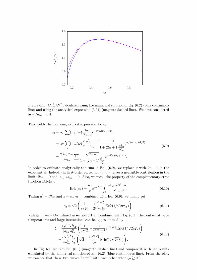
0.7
0.9
1.1
1.3
1.5
0.2 0.4 0.6 0.8
Ca3 ho/N
2
ξT
Figure 6.1: Ca3ho/N
2 calculated using the numerical solution of Eq. (6.2) (blue continuousline) and using the analytical expression (3.54) (magenta dashed line). We have considered|a1D|/aho = 0.4.
This yields the following explicit expression for c2:
c2 = λT∑ν
(−β~ω)∂ν
∂|a1D|e−β~ω(νn+1/2)
= λT∑n
(−β~ω)2
π
√2n+ 1
aho
−1
1 + (2n+ 1)a21Da2ho
e−β~ω(νn+1/2)
=2λTβ~ωπaho
∑n
√2n+ 1
1 + (2n+ 1)a21Da2ho
e−β~ω(νn+1/2).
(6.9)
In order to evaluate analytically the sum in Eq. (6.9), we replace ν with 2n + 1 in theexponential. Indeed, the first-order correction in |a1D| gives a negligible contribution in thelimit β~ω → 0 and |a1D|/aho → 0. Also, we recall the property of the complementary errorfunction Erfc(x),
Erfc(az) =2z
πe−a
2z2∫ +∞
0
e−a2t2 dt
t2 + z2. (6.10)
Taking a2 = β~ω and z = aho/a1D, combined with Eq. (6.9), we finally get
c2 =√
2
(1
2πξ2T
− e1/2πξ2T
23/2πξ3T
Erfc(1/√
2πξT)
). (6.11)
with ξT = −a1D/λT defined in section 3.1.1. Combined with Eq. (6.1), the contact at largetemperatures and large interactions can be approximated by
C =4√
2N2ξT|a1D|a2
ho
(1
2πξ2T
− 1
23/2πξ3T
e1/2πξ2TErfc(1/√
2πξT)
)=
2N5/2
πa3ho
ξγξT
(√
2− e1/2πξ2T
ξTErfc(1/
√2πξT)
).
(6.12)
In Fig. 6.1, we plot Eq. (6.1) (magenta dashed line) and compare it with the resultscalculated by the numerical solution of Eq. (6.2) (blue continuouus line). From the plot,we can see that these two curves fit well with each other when ξT & 0.3.

List of publications
1. H. Yao, D. Clément, A. Minguzzi, P. Vignolo and L. Sanchez-Palencia. ”Tan’scontact for trapped Lieb-Liniger bosons at finite temperature”, Phys. Rev. Lett.121,220402 (2018).
2. H. Yao, H. Khoudli, L. Bresque and L. Sanchez-Palencia. ”Critical behavior andfractality in shallow one-dimensional quasiperiodic potentials”, Phys. Rev. Lett. 123,070405 (2019).
3 H. Yao, T. Giamarchi, and L. Sanchez-Palencia, ”Lieb-Liniger bosons in a shallowquasiperiodic potential: Bose glass phase and fractal Mott lobes”, Phys. Rev. Lett.125, 060401 (2020).
4. R. Gautier, H. Yao and L. Sanchez-Palencia. ”Strongly-Interacting bosons in atwo-dimensional quasicrystal lattice”, arXiv : 2010.07590 (2020)
130
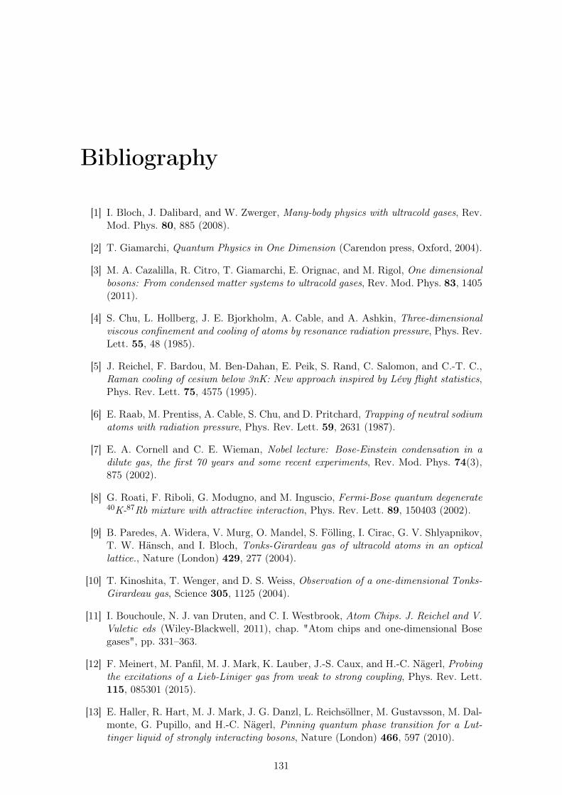
Bibliography
[1] I. Bloch, J. Dalibard, and W. Zwerger, Many-body physics with ultracold gases, Rev.Mod. Phys. 80, 885 (2008).
[2] T. Giamarchi, Quantum Physics in One Dimension (Carendon press, Oxford, 2004).
[3] M. A. Cazalilla, R. Citro, T. Giamarchi, E. Orignac, and M. Rigol, One dimensionalbosons: From condensed matter systems to ultracold gases, Rev. Mod. Phys. 83, 1405(2011).
[4] S. Chu, L. Hollberg, J. E. Bjorkholm, A. Cable, and A. Ashkin, Three-dimensionalviscous confinement and cooling of atoms by resonance radiation pressure, Phys. Rev.Lett. 55, 48 (1985).
[5] J. Reichel, F. Bardou, M. Ben-Dahan, E. Peik, S. Rand, C. Salomon, and C.-T. C.,Raman cooling of cesium below 3nK: New approach inspired by Lévy flight statistics,Phys. Rev. Lett. 75, 4575 (1995).
[6] E. Raab, M. Prentiss, A. Cable, S. Chu, and D. Pritchard, Trapping of neutral sodiumatoms with radiation pressure, Phys. Rev. Lett. 59, 2631 (1987).
[7] E. A. Cornell and C. E. Wieman, Nobel lecture: Bose-Einstein condensation in adilute gas, the first 70 years and some recent experiments, Rev. Mod. Phys. 74(3),875 (2002).
[8] G. Roati, F. Riboli, G. Modugno, and M. Inguscio, Fermi-Bose quantum degenerate40K-87Rb mixture with attractive interaction, Phys. Rev. Lett. 89, 150403 (2002).
[9] B. Paredes, A. Widera, V. Murg, O. Mandel, S. Fölling, I. Cirac, G. V. Shlyapnikov,T. W. Hänsch, and I. Bloch, Tonks-Girardeau gas of ultracold atoms in an opticallattice., Nature (London) 429, 277 (2004).
[10] T. Kinoshita, T. Wenger, and D. S. Weiss, Observation of a one-dimensional Tonks-Girardeau gas, Science 305, 1125 (2004).
[11] I. Bouchoule, N. J. van Druten, and C. I. Westbrook, Atom Chips. J. Reichel and V.Vuletic eds (Wiley-Blackwell, 2011), chap. "Atom chips and one-dimensional Bosegases", pp. 331–363.
[12] F. Meinert, M. Panfil, M. J. Mark, K. Lauber, J.-S. Caux, and H.-C. Nägerl, Probingthe excitations of a Lieb-Liniger gas from weak to strong coupling, Phys. Rev. Lett.115, 085301 (2015).
[13] E. Haller, R. Hart, M. J. Mark, J. G. Danzl, L. Reichsöllner, M. Gustavsson, M. Dal-monte, G. Pupillo, and H.-C. Nägerl, Pinning quantum phase transition for a Lut-tinger liquid of strongly interacting bosons, Nature (London) 466, 597 (2010).
131
[14] C. D’Errico, E. Lucioni, L. Tanzi, L. Gori, G. Roux, I. P. McCulloch, T. Giamarchi,M. Inguscio, and G. Modugno, Observation of a disordered bosonic insulator fromweak to strong interactions, Phys. Rev. Lett. 113, 095301 (2014).
[15] G. Boéris, L. Gori, M. D. Hoogerland, A. Kumar, E. Lucioni, L. Tanzi, M. Inguscio,T. Giamarchi, C. D’Errico, G. Carleo, et al., Mott transition for strongly interactingone-dimensional bosons in a shallow periodic potential, Phys. Rev. A 93, 011601(R)(2016).
[16] T. Kohlert, S. Scherg, X. Li, H. P. Lüschen, S. Das Sarma, I. Bloch, and M. Aidels-burger, Observation of many-body localization in a one-dimensional system with asingle-particle mobility edge, Phys. Rev. Lett. 122, 170403 (2019).
[17] A. Minguzzi, P. Vignolo, and M. Tosi, High momentum tail in the Tonks gas underharmonic confinement, J. Phys. Lett. A 294, 222 (2002).
[18] P. Vignolo and A. Minguzzi, Universal contact for a Tonks-Girardeau gas at finitetemperature, Phys. Rev. Lett. 110, 020403 (2013).
[19] K. Viebahn, M. Sbroscia, E. Carter, J.-C. Yu, and U. Schneider, Matter-wave diffrac-tion from a quasicrystalline optical lattice, Phys. Rev. Lett. 122, 110404 (2019).
[20] L. Fallani, J. E. Lye, V. Guarrera, C. Fort, and M. Inguscio, Ultracold atoms in adisordered crystal of light: Towards a Bose glass, Phys. Rev. Lett. 98, 130404 (2007).
[21] L. Tanzi, E. Lucioni, S. Chaudhuri, L. Gori, A. Kumar, C. D’Errico, M. Inguscio, andG. Modugno, Transport of a Bose gas in 1D disordered lattices at the fluid-insulatortransition, Phys. Rev. Lett. 111, 115301 (2013).
[22] P. Lugan, D. Clément, P. Bouyer, A. Aspect, M. Lewenstein, and L. Sanchez-Palencia, Ultracold Bose gases in 1D disorder: From Lifshits glass to Bose-Einsteincondensate, Phys. Rev. Lett. 98, 170403 (2007).
[23] G. Roux, T. Barthel, I. P. McCulloch, C. Kollath, U. Schollwöck, and T. Giamarchi,Quasiperiodic Bose-hubbard model and localization in one-dimensional cold atomicgases, Phys. Rev. A 78(2), 023628 (2008).
[24] L. Gori, T. Barthel, A. Kumar, E. Lucioni, L. Tanzi, M. Inguscio, G. Modugno,T. Giamarchi, C. D’Errico, and G. Roux, Finite-temperature effects on interactingbosonic one-dimensional systems in disordered lattices, Phys. Rev. A 93, 033650(2016).
[25] L. Pricoupenko and M. Olshanii, Stability of two-dimensional Bose gases in the res-onant regime, J. Phys. B: At. Mol. Opt. Phys. 40, 2065 (2007).
[26] C. Mora and Y. Castin, Extension of bogoliubov theory to quasicondensates, Phys.Rev. A 67(5), 053615 (2003).
[27] Z. Hadzibabic and J. Dalibard, Two-dimensional Bose fluids: An atomic physicsperspective, Rivista del Nuovo Cimento 34, 389 (2011).
[28] G. Carleo, G. Boéris, M. Holzmann, and L. Sanchez-Palencia, Universal superfluidtransition and transport properties of two-dimensional dirty bosons, Phys. Rev. Lett.111, 050406 (2013).
[29] L.-C. Ha, C.-L. Hung, X. Zhang, U. Eismann, S.-K. Tung, and C. Chin, Stronglyinteracting two-dimensional bose gases, Phys. Rev. Lett. 110(14), 145302 (2013).

[30] C. De Rossi, R. Dubessy, K. Merloti, M. d. G. de Herve, T. Badr, A. Perrin,L. Longchambon, and H. Perrin, Probing superfluidity in a quasi two-dimensionalbose gas through its local dynamics, New J. Phys. 18(6), 062001 (2016).
[31] A. Szabó and U. Schneider, Non-power-law universality in one-dimensional qua-sicrystals, Phys. Rev. B 98, 134201 (2018).
[32] A. Szabó and U. Schneider, Mixed spectra and partially extended states in a two-dimensional quasiperiodic model, Phys. Rev. B 101(1), 014205 (2020).
[33] M. Sbroscia, K. Viebahn, E. Carter, J.-C. Yu, A. Gaunt, and U. Schneider, Observinglocalisation in a 2D quasicrystalline optical lattice, arXiv preprint arXiv:2001.10912(2020).
[34] F. Meinert, M. Knap, E. Kirilov, K. Jag-Lauber, M. B. Zvonarev, E. Demler, andH.-C. Nägerl, Bloch oscillations in the absence of a lattice, Science 356(6341), 945(2017).
[35] G. Lang, F. Hekking, and A. Minguzzi, Ground-state energy and excitation spectrumof the lieb-liniger model: accurate analytical results and conjectures about the exactsolution, SciPost Physics 3(1), 003 (2017).
[36] J. Despres, L. Villa, and L. Sanchez-Palencia, Twofold correlation spreading in astrongly correlated lattice Bose gas, Sci. Rep. 9, 4135 (2019).
[37] L. Villa, J. Despres, and L. Sanchez-Palencia, Unraveling the excitation spectrum ofmany-body systems from quantum quenches, Phys. Rev. A 100, 063632 (2019).
[38] L. Villa, J. Despres, S. Thomson, and L. Sanchez-Palencia, Local quench spectroscopyof many-body quantum systems, arXiv preprint arXiv:2007.08381 (2020).
[39] Y. Guo, R. Dubessy, M. d. G. de Herve, A. Kumar, T. Badr, A. Perrin, L. Longcham-bon, and H. Perrin, Supersonic rotation of a superfluid: a long-lived dynamical ring,Phys. Rev. Lett. 124(2), 025301 (2020).
[40] M. Girardeau, Relationship between systems of impenetrable bosons and fermions inone dimension, J. Math. Phys. 1, 516 (1960).
[41] S. Lellouch and L. Sanchez-Palencia, Localization transition in weakly-interactingBose superfluids in one-dimensional quasiperdiodic lattices, Phys. Rev. A 90,061602(R) (2014).
[42] D. Jaksch, C. Bruder, J. I. Cirac, C. W. Gardiner, and P. Zoller, Cold bosonic atomsin optical lattices, Phys. Rev. Lett. 81(15), 3108 (1998).
[43] M. Greiner, O. Mandel, T. Esslinger, T. W. Hänsch, and I. Bloch, Quantum phasetransition from a superfluid to a Mott insulator in a gas of ultracold atoms, Nature(London) 415(6867), 39 (2002).
[44] S. Inouye, M. R. Andrews, J. Stenger, H. J. Miesner, D. M. Stamper-Kurn, andW. Ketterle, Observation of Feshbach resonances in a Bose-Einstein condensate,Nature (London) 392(6672), 151 (1998).
[45] S. L. Cornish, N. R. Claussen, J. L. Roberts, E. A. Cornell, and C. E. Wieman,Stable 85Rb Bose-Einstein condensates with widely tunable interactions, Phys. Rev.Lett. 85(9), 1795 (2000).

[46] V. Gurarie and J. T. Chalker, Some generic aspects of bosonic excitations in disor-dered systems, Phys. Rev. Lett. 89, 136801 (2002).
[47] V. Gurarie, G. Refael, and J. T. Chalker, Excitations of one-dimensional Bose-Einstein condensates in a random potential, Phys. Rev. Lett. 101(17), 170407 (2008).
[48] N. Bilas and N. Pavloff, Anderson localization of elementary excitations in a one-dimensional Bose-Einstein condensate, Eur. Phys. J. D 40(3), 387 (2006).
[49] P. Lugan, D. Clément, P. Bouyer, A. Aspect, and L. Sanchez-Palencia, Andersonlocalization of Bogolyubov quasiparticles in interacting Bose-Einstein condensates,Phys. Rev. Lett. 99(18), 180402 (2007).
[50] P. Lugan and L. Sanchez-Palencia, Localization of Bogoliubov quasiparticles in inter-acting Bose gases with correlated disorder, Phys. Rev. A 84(1), 013612 (2011).
[51] S. Lellouch, L.-K. Lim, and L. Sanchez-Palencia, Propagation of collective pair exci-tations in disordered Bose superfluids, Phys. Rev. A 92, 043611 (2015).
[52] T. Giamarchi and H. J. Schulz, Localization and interactions in one-dimensionalquantum fluids, Europhys. Lett. 3, 1287 (1987).
[53] T. Giamarchi and H. J. Schulz, Anderson localization and interactions in one-dimensional metals, Phys. Rev. B 37(1), 325 (1988).
[54] M. P. A. Fisher, P. B. Weichman, G. Grinstein, and D. S. Fisher, Boson localizationand the superfluid-insulator transition, Phys. Rev. B 40(1), 546 (1989).
[55] E. H. Lieb and W. Liniger, Exact analysis of an interacting Bose gas. I. The generalsolution and the ground state, Phys. Rev. 130, 1605 (1963).
[56] E. H. Lieb, Exact analysis of an interacting Bose gas. II. The excitation spectrum,Phys. Rev. 130, 1616 (1963).
[57] C. N. Yang and C. P. Yang, Thermodynamics of a one-dimensional system of bosonswith repulsive δ-function interaction, J. Math. Phys. 10, 1115 (1969).
[58] M. Boninsegni, N. Prokof’ev, and B. Svistunov, Worm algorithm for continuous-spacepath integral Monte Carlo simulations, Phys. Rev. Lett. 96, 070601 (2006).
[59] M. Boninsegni, N. V. Prokof’ev, and B. V. Svistunov, Worm algorithm and diagram-matic Monte Carlo: A new approach to continuous-space path integral Monte Carlosimulations, Phys. Rev. E 74, 036701 (2006).
[60] V. Gurarie, One-dimensional gas of bosons with Feshbach-resonant interactions,Phys. Rev. A 73(3), 033612 (2006).
[61] N. Fabbri, M. Panfil, D. Clément, L. Fallani, M. Inguscio, C. Fort, and J.-S. Caux,Dynamical structure factor of one-dimensional Bose gases: Experimental signaturesof beyond-Luttinger-liquid physics, Phys. Rev. A 91, 043617 (2015).
[62] M. Olshanii, Atomic scattering in the presence of an external confinement and a gasof impenetrable bosons, Phys. Rev. Lett. 81(5), 938 (1998).
[63] V. Flambaum, G. Gribakin, and C. Harabati, Analytical calculation of cold-atomscattering, Phys. Rev. A 59(3), 1998 (1999).

[64] S. Dettmer, D. Hellweg, P. Ryytty, J. J. Arlt, W. Ertmer, K. Sengstock, D. S.Petrov, G. V. Shlyapnikov, H. Kreutzmann, L. Santos, et al., Observation of phasefluctuations in elongated Bose-Einstein condensates, Phys. Rev. Lett. 87, 160406(2001).
[65] F. Gerbier, J. H. Thywissen, S. Richard, M. Hugbart, P. Bouyer, and A. Aspect,Momentum distribution and correlation function of quasicondensates in elongatedtraps, Phys. Rev. A 67, 051602 (2003).
[66] J. Estève, J.-B. Trebbia, T. Schumm, A. Aspect, C. I. Westbrook, and I. Bouchoule,Observations of density fluctuations in an elongated Bose gas: Ideal gas and quasi-condensate regimes, Phys. Rev. Lett. 96, 130403 (2006).
[67] J. Decamp, M. Albert, and P. Vignolo, Tan’s contact in a cigar-shaped dilute bosegas, Phys. Rev. A 97(3), 033611 (2018).
[68] T. NAGAMIYA, Statistical mechanics of one-dimensional substances i, Proceedingsof the Physico-Mathematical Society of Japan. 3rd Series 22(8-9), 705 (1940).
[69] G. De Rosi, P. Massignan, M. Lewenstein, and G. E. Astrakharchik, Beyond-Luttinger-liquid thermodynamics of a one-dimensional bose gas with repulsive contactinteractions, Phys. Rev. R 1(3), 033083 (2019).
[70] D. S. Petrov, G. V. Shlyapnikov, and J. T. M. Walraven, Regimes of quantum de-generacy in trapped 1D gases, Phys. Rev. Lett. 85, 3745 (2000).
[71] A. O. gogolin, A. A. Nersesyan, and A. M. Tsvelik, Bosonization and strongly corre-lated systems (Cambridge university press, 2004).
[72] F. D. M. Haldane, Effective harmonic-fluid approach to low-energy properties of one-dimensional quantum fluids, Phys. Rev. Lett. 47, 1840 (1981).
[73] G. G. Batrouni, R. T. Scalettar, and G. T. Zimanyi, Quantum critical phenomenain one-dimensional Bose systems, Phys. Rev. Lett. 65, 1765 (1990).
[74] V. A. Kashurnikov, A. V. Krasavin, and B. V. Svistunov, Mott-insulator-superfluid-liquid transition in a one-dimensional bosonic hubbard model: Quantum monte carlomethod, JETP Lett. 64(2), 99 (1996).
[75] T. D. Kühner and H. Monien, Phases of the one-dimensional Bose-Hubbard model,Phys. Rev. B 58, R14741 (1998).
[76] T. D. Kühner, S. R. White, and H. Monien, One-dimensional Bose-Hubbard modelwith nearest-neighbor interaction, Phys. Rev. B 61, 12474 (2000).
[77] N. Elstner and H. Monien, Dynamics and thermodynamics of the bose-hubbard model,Phys. Rev. B 59(19), 12184 (1999).
[78] V. Pokrovsky and A. Talapov, Ground state, spectrum, and phase diagram of two-dimensional incommensurate crystals, Phys. Rev. Lett. 42(1), 65 (1979).
[79] H. J. Schulz, Critical behavior of commensurate-incommensurate phase transitions intwo dimensions, Phys. Rev. B 22, 5274 (1980).
[80] T. Giamarchi, Resistivity of a one-dimensional interacting quantum fluid, Phys. Rev.B 46, 342 (1992).

[81] E. B. Kolomeisky, Universal jumps of conductance at the metal-insulator transitionin one dimension, Phys. Rev. B 47, 6193 (1993).
[82] H.-P. Büchler, G. Blatter, and W. Zwerger, Commensurate-incommensurate transi-tion of cold atoms in an optical lattice, Phys. Rev. Lett. 90(13), 130401 (2003).
[83] S. Rapsch, U. Schollwöck, and W. Zwerger, Density matrix renormalization groupfor disordered bosons in one dimension, Europhys. Lett. 46, 559 (1999).
[84] L. Fontanesi, M. Wouters, and V. Savona, Superfluid to Bose-glass transition in a1d weakly interacting Bose gas, Phys. Rev. Lett. 103(3), 030403 (2009).
[85] L. Pollet, N. V. Prokof’ev, B. V. Svistunov, and M. Troyer, Absence of a directsuperfluid to Mott insulator transition in disordered Bose systems, Phys. Rev. Lett.103(14), 140402 (2009).
[86] H. Yao, H. Khoudli, L. Bresque, and L. Sanchez-Palencia, Critical behavior andfractality in shallow one-dimensional quasiperiodic potentials, Phys. Rev. Lett. 123,070405 (2019).
[87] A. Lüscher and A. M. Läuchli, Exact diagonalization study of the antiferromagneticspin-1/2 heisenberg model on the square lattice in a magnetic field, Phys. Rev. B79(19), 195102 (2009).
[88] A. M. Läuchli, J. Sudan, and E. S. Sørensen, Ground-state energy and spin gap ofspin-1/2 kagomé-heisenberg antiferromagnetic clusters: Large-scale exact diagonal-ization results, Phys. Rev. B 83(21), 212401 (2011).
[89] E. P. Gross, Structure of a quantized vortex in boson systems, Il Nuovo Cimento(1955-1965) 20(3), 454 (1961).
[90] L. P. Pitaevskii, Vortex lines in an imperfect bose gas, Sov. Phys. JETP 13(2), 451(1961).
[91] N. Bogoliubov, On the theory of superfluidity, J. Phys 11(1), 23 (1947).
[92] L. Pollet, Recent developments in quantum monte carlo simulations with applicationsfor cold gases, Reports on progress in physics 75(9), 094501 (2012).
[93] W. L. McMillan, Ground state of liquid he 4, Phys. Rev. 138(2A), A442 (1965).
[94] D. Ceperley, G. Chester, and M. Kalos, Monte carlo simulation of a many-fermionstudy, Phys. Rev. B 16(7), 3081 (1977).
[95] J. W. Moskowitz, K. Schmidt, M. A. Lee, and M. H. Kalos, A new look at correlationenergy in atomic and molecular systems. ii. the application of the green’s functionmonte carlo method to LiH, The Journal of chemical physics 77(1), 349 (1982).
[96] P. J. Reynolds, D. M. Ceperley, B. J. Alder, and W. A. Lester Jr, Fixed-node quantummonte carlo for molecules, The Journal of Chemical Physics 77(11), 5593 (1982).
[97] E. Pollock and D. M. Ceperley, Simulation of quantum many-body systems by path-integral methods, Phys. Rev. B 30(5), 2555 (1984).
[98] E. Pollock and D. M. Ceperley, Path-integral computation of superfluid densities,Phys. Rev. B 36(16), 8343 (1987).

[99] D. M. Ceperley, Path integrals in the theory of condensed helium, Rev. Mod. Phys.67, 279 (1995).
[100] N. Prokof’ev and B. Svistunov, Bold diagrammatic Monte Carlo technique: when thesign problem is welcome, Phys. Rev. Lett. 99, 250201 (2007).
[101] G. Carleo, F. Becca, M. Schiró, and M. Fabrizio, Localization and glassy dynamicsof many-body quantum systems, Sci. Rep. 2, 243 (2012).
[102] G. Carleo, L. Cevolani, L. Sanchez-Palencia, and M. Holzmann, Unitary dynamicsof strongly interacting Bose gases with the time-dependent variational Monte Carlomethod in continuous space, Phys. Rev. X 7, 031026 (2017).
[103] N. Wiener, The average of an analytic functional, Proceedings of the NationalAcademy of Sciences of the United States of America 7(9), 253 (1921).
[104] N. Wiener, Differential-space, Journal of Mathematics and Physics 2(1-4), 131(1923).
[105] P. DIRAC, The lagrangian in quantum mechanics, Physikalische Zeitschirift der Sow-jetunion 3, 312 (1933).
[106] R. P. Feynman, Space-time approach to nonrelativistic quantum mechanics, Rev.Mod. Phys. 20, 367 (1948).
[107] M. Kac, On distributions of certain wiener functionals, Transactions of the AmericanMathematical Society 65(1), 1 (1949).
[108] H. F. Trotter, On the product of semi-groups of operators, Proceedings of the Amer-ican Mathematical Society 10(4), 545 (1959).
[109] M. Suzuki, Generalized trotter’s formula and systematic approximants of exponentialoperators and inner derivations with applications to many-body problems, Communi-cations in Mathematical Physics 51(2), 183 (1976).
[110] J. Barker, A quantum-statistical monte carlo method; path integrals with boundaryconditions, The Journal of Chemical Physics 70(6), 2914 (1979).
[111] Y. Yan and D. Blume, Incorporating exact two-body propagators for zero-range in-teractions into n-body monte carlo simulations, Phys. Rev. A 91(4), 043607 (2015).
[112] W. Krauth, Statistical mechanics: algorithms and computations, vol. 13 (OUP Ox-ford, 2006).
[113] M. Pierce and E. Manousakis, Path-integral monte carlo simulation of the secondlayer of 4 he adsorbed on graphite, Physical Review B 59(5), 3802 (1999).
[114] N. Metropolis, A. W. Rosenbluth, M. N. Rosenbluth, A. H. Teller, and E. Teller,Equation of state calculations by fast computing machines, The journal of chemicalphysics 21(6), 1087 (1953).
[115] W. HASTINGS, Monte carlo sampling methods using marcov chains and their appli-cations, Biometrika 57, 97 (1970).
[116] V. Ambegaokar and M. Troyer, Estimating errors reliably in monte carlo simulationsof the ehrenfest model, American Journal of Physics 78(2), 150 (2010).

[117] B. Bauer, L. Carr, H. G. Evertz, A. Feiguin, J. Freire, S. Fuchs, L. Gamper, J. Gukel-berger, E. Gull, S. Guertler, et al., The alps project release 2.0: open source softwarefor strongly correlated systems, Journal of Statistical Mechanics: Theory and Exper-iment 2011(05), P05001 (2011).
[118] M. Troyer, B. Ammon, and E. Heeb, in International Symposium on Computing inObject-Oriented Parallel Environments, Springer (1998), pp. 191–198.
[119] W. Krauth, Quantum monte carlo calculations for a large number of bosons in aharmonic trap, Phys. Rev. Lett. 77(18), 3695 (1996).
[120] M. Holzmann and W. Krauth, Kosterlitz-thouless transition of the quasi-two-dimensional trapped bose gas, Phys. Rev. Lett. 100(19), 190402 (2008).
[121] M. Olshanii and V. Dunjko, Short-distance correlation properties of the Lieb-Linigersystem and momentum distributions of trapped one-dimensional atomic gases, Phys.Rev. Lett. 91, 090401 (2003).
[122] S. Tan, Large momentum part of fermions with large scattering length, Ann. Phys.(NY) 323, 2971 (2008).
[123] S. Tan, Generalized virial theorem and pressure relation for a strongly correlatedFermi gas, Ann. Phys. (NY) 323, 2987 (2008).
[124] S. Tan, Energetics of a strongly correlated Fermi gas, Ann. Phys. (NY) 323, 2952(2008).
[125] R. Chang, Q. Bouton, H. Cayla, C. Qu, A. Aspect, C. I. Westbrook, and D. Clément,Momentum-resolved observation of thermal and quantum depletion in a Bose gas,Phys. Rev. Lett. 117, 235303 (2016).
[126] R. J. Wild, P. Makotyn, J. M. Pino, E. A. Cornell, and D. S. Jin, Measurements ofTan’s contact in an atomic Bose-Einstein condensate, Phys. Rev. Lett. 108, 145305(2012).
[127] J. T. Stewart, J. P. Gaebler, T. E. Drake, and D. S. Jin, Verification of universalrelations in a strongly interacting Fermi gas, Phys. Rev. Lett. 104, 235301 (2010).
[128] Y. Sagi, T. E. Drake, R. Paudel, and D. S. Jin, Measurement of the homogeneouscontact of a unitary Fermi gas, Phys. Rev. Lett. 109, 220402 (2012).
[129] S. Hoinka, M. Lingham, K. Fenech, H. Hu, C. J. Vale, J. E. Drut, and S. Gandolfi,Precise determination of the structure factor and contact in a unitary Fermi gas,Phys. Rev. Lett. 110, 055305 (2013).
[130] C. Luciuk, S. Trotzky, S. Smale, Z. Yu, S. Zhang, and J. H. Thywissen, Evidencefor universal relations describing a gas with p-wave interactions, Nat. Phys. 12, 599(2016).
[131] R. J. Fletcher, R. Lopes, J. Man, N. Navon, R. P. Smith, M. W. Zwierlein, andZ. Hadzibabic, Two- and three-body contacts in the unitary Bose gas, Science 355,377 (2017).
[132] S. Laurent, M. Pierce, M. Delehaye, T. Yefsah, F. Chevy, and C. Salomon, Connectingfew-body inelastic decay to quantum correlations in a many-body system: A weaklycoupled impurity in a resonant Fermi gas, Phys. Rev. Lett. 118, 103403 (2017).

[133] A. Johnson, S. S. Szigeti, M. Schemmer, and I. Bouchoule, Long-lived nonthermalstates realized by atom losses in one-dimensional quasicondensates, Phys. Rev. A 96,013623 (2017).
[134] K. V. Kheruntsyan, D. M. Gangardt, P. D. Drummond, and G. V. Shlyapnikov, Paircorrelations in a finite-temperature 1D Bose gas, Phys. Rev. Lett. 91, 040403 (2003).
[135] M. Kormos, G. Mussardo, and A. Trombettoni, Expectation values in the Lieb-LinigerBose gas, Phys. Rev. Lett. 103, 210404 (2009).
[136] W. Xu and M. Rigol, Universal scaling of density and momentum distributions inLieb-Liniger gases, Phys. Rev. A 92, 063623 (2015).
[137] H. Yao, D. Clément, A. Minguzzi, P. Vignolo, and L. Sanchez-Palencia, Tan’s contactfor trapped Lieb-Liniger bosons at finite temperature, Phys. Rev. Lett. 121, 220402(2018).
[138] M. Barth and W. Zwerger, Tan relations in one dimension, Ann. Phys. (NY) 326,2544 (2011).
[139] M. A. Cazalilla, One-dimensional optical lattices and impenetrable bosons, Phys. Rev.A 67, 053606 (2003).
[140] H. Hu, X.-J. Liu, and P. D. Drummond, Universal contact of strongly interactingfermions at finite temperatures, New J. Phys. 13(3), 035007 (2011).
[141] X.-J. Liu, H. Hu, and P. D. Drummond, Virial expansion for a strongly correlatedFermi gas, Phys. Rev. Lett. 102(16), 160401 (2009).
[142] T. Busch, B.-G. Englert, K. Rzażewski, and M. Wilkens, Two cold atoms in a har-monic trap, Foundations of Physics 28(4), 549 (1998).
[143] P. W. Anderson, Absence of diffusion in certain random lattices, Phys. Rev. 109,1492 (1958).
[144] E. Abrahams, 50 years of Anderson Localization (World Scientific, Singapore, 2010).
[145] P. A. Lee and T. V. Ramakrishnan, Disordered electronic systems, Rev. Mod. Phys.57(2), 287 (1985).
[146] D. S. Wiersma, P. Bartolini, A. Lagendijk, and R. Righini, Localization of light in adisordered medium, Nature (London) 390, 671 (1997).
[147] M. Störzer, P. Gross, C. M. Aegerter, and G. Maret, Observation of the criticalregime near Anderson localization of light, Phys. Rev. Lett. 96(6), 063904 (2006).
[148] T. Schwartz, G. Bartal, S. Fishman, and M. Segev, Transport and Anderson local-ization in disordered two-dimensional photonic lattices, Nature (London) 446, 52(2007).
[149] V. Gurarie and J. T. Chalker, Bosonic excitations in random media, Phys. Rev. B68(13), 134207 (2003).
[150] P. W. Anderson, Theory of dirty superconductors, J. Phys. Chem. Sol. 11, 26 (1959).
[151] G. Orso, BCS-BEC crossover in a random external potential, Phys. Rev. Lett. 99(25),250402 (2007).

[152] L. Han and C. A. R. Sá de Melo, Evolution from Bardeen-Cooper-Schrieffer to Bose-Einstein condensate superfluidity in the presence of disorder, New J. Phys. 13(5),055012 (2011).
[153] L. Sanchez-Palencia and M. Lewenstein, Disordered quantum gases under control,Nat. Phys. 6, 87 (2010).
[154] D. Shechtman, I. Blech, D. Gratias, and J. W. Cahn, Metallic phase with long-rangeorientational order and no translational symmetry, Phys. Rev. Lett. 53, 1951 (1984).
[155] R. Peierls, Theory of the diamagnetism of conduction electrons, Z. Phys. 80, 763(1933).
[156] P. G. Harper, Single band motion of conduction electrons in a uniform magnetic field,Proc. Phys. Soc. London A 68, 874 (1955).
[157] D. R. Hofstadter, Energy levels and wave functions of Bloch electrons in rational andirrational magnetic fields, Phys. Rev. B 14, 2239 (1976).
[158] J. Wilson, F. Di Salvo, and S. Mahajan, Charge-density waves and superlattices inthe metallic layered transition metal dichalcogenides, Adv. Phys. 24, 117 (1975).
[159] R. Merlin, K. Bajema, R. Clarke, F. Y. Juang, and P. K. Bhattacharya, QuasiperiodicGaAs-AlAs heterostructures, Phys. Rev. Lett. 55, 1768 (1985).
[160] Y. Lahini, R. Pugatch, F. Pozzi, M. Sorel, R. Morandotti, N. Davidson, and Y. Sil-berberg, Observation of a localization transition in quasiperiodic photonic lattices,Phys. Rev. Lett. 103, 013901 (2009).
[161] D. Tanese, E. Gurevich, F. Baboux, T. Jacqmin, A. Lemaître, E. Galopin, I. Sagnes,A. Amo, J. Bloch, and E. Akkermans, Fractal energy spectrum of a polariton gas ina Fibonacci quasiperiodic potential, Phys. Rev. Lett. 112, 146404 (2014).
[162] A. Aspect and M. Inguscio, Anderson localization of ultracold atoms, Phys. Today62, 30 (2009).
[163] G. Modugno, Anderson localization in Bose-Einstein condensates, Rep. Prog. Phys.73, 102401 (2010).
[164] B. Damski, J. Zakrzewski, L. Santos, P. Zoller, and M. Lewenstein, Atomic Bose andAnderson glasses in optical lattices, Phys. Rev. Lett. 91, 080403 (2003).
[165] R. Roth and K. Burnett, Phase diagram of bosonic atoms in two-color superlattices,Phys. Rev. A 68, 023604 (2003).
[166] L. Sanchez-Palencia and L. Santos, Bose-Einstein condensates in optical quasicrystallattices, Phys. Rev. A 72, 053607 (2005).
[167] N. Macé, A. Jagannathan, and M. Duneau, Quantum simulation of a 2D quasicrystalwith cold atoms, Crystals 6, 124 (2016).
[168] B. Gadway, D. Pertot, J. Reeves, M. Vogt, and D. Schneble, Glassy behavior in abinary atomic mixture, Phys. Rev. Lett. 107, 145306 (2011).
[169] S. Iyer, V. Oganesyan, G. Refael, and D. A. Huse, Many-body localization in aquasiperiodic system, Phys. Rev. B 87, 134202 (2013).

[170] A. Lukin, M. Rispoli, R. Schittko, M. E. Tai, A. M. Kaufman, S. Choi, V. Khemani,J. Léonard, and M. Greiner, Probing entanglement in a many-body-localized system,arXiv:1805.09819 (2018).
[171] R. Matthew, L. Alexander, S. Robert, K. Sooshin, T. M. Eric, L. Julian, andG. Markus, Quantum critical behavior at the many-body-localization transition,arXiv:1812.06959 (2018).
[172] E. Abrahams, P. W. Anderson, D. C. Licciardello, and T. V. Ramakrishnan, Scalingtheory of localization: Absence of quantum diffusion in two dimensions, Phys. Rev.Lett. 42, 673 (1979).
[173] S. Aubry and G. André, Analyticity breaking and Anderson localization in incom-mensurate lattices, Ann. Israel Phys. Soc. 3, 133 (1980).
[174] C. Soukoulis and E. Economou, Localization in one-dimensional lattices in the pres-ence of incommensurate potentials, Phys. Rev. Lett. 48, 1043 (1982).
[175] S. Das Sarma, A. Kobayashi, and R. E. Prange, Proposed experimental realizationof Anderson localization in random and incommensurate artificially layered systems,Phys. Rev. Lett. 56, 1280 (1986).
[176] J. Biddle, B. Wang, D. J. Priour Jr, and S. Das Sarma, Localization in one-dimensional incommensurate lattices beyond the Aubry-André model, Phys. Rev. A80, 021603 (2009).
[177] J. Biddle and S. Das Sarma, Predicted mobility edges in one-dimensional incommen-surate optical lattices: An exactly solvable model of Anderson localization, Phys. Rev.Lett. 104, 070601 (2010).
[178] J. Biddle, D. J. Priour Jr, B. Wang, and S. D. Sarma, Localization in one-dimensionallattices with non-nearest-neighbor hopping : Generalized Anderson and Aubry-Andrémodels, Phys. Rev. B 83, 075105 (2011).
[179] S. Ganeshan, J. Pixley, and S. Das Sarma, Nearest neighbor tight binding models withan exact mobility edge in one dimension, Phys. Rev. Lett. 114, 146601 (2015).
[180] D. J. Boers, B. Goedeke, D. Hinrichs, and M. Holthaus, Mobility edges in bichromaticoptical lattices, Phys. Rev. A 75, 063404 (2007).
[181] X. Li, X. Li, and S. Das Sarma, Mobility edges in one-dimensional bichromatic in-commensurate potentials, Phys. Rev. B 96, 085119 (2017).
[182] H. P. Lüschen, S. Scherg, T. Kohlert, M. Schreiber, P. Bordia, X. Li, S. Das Sarma,and I. Bloch, Single-particle mobility edge in a one-dimensional quasiperiodic opticallattice, Phys. Rev. Lett. 120, 160404 (2018).
[183] F. Evers and A. D. Mirlin, Anderson transitions, Rev. Mod. Phys. 80, 1355 (2008).
[184] R. B. Diener, G. A. Georgakis, J. Zhong, M. Raizen, and Q. Niu, Transition betweenextended and localized states in a one-dimensional incommensurate optical lattice,Phys. Rev. A 64(3), 033416 (2001).
[185] A. Avila and S. Jitomirskaya, The ten martini problem, Annals of Mathematics pp.303–342 (2009).
[186] I. M. Lifshits, S. Gredeskul, and L. Pastur, Introduction to the Theory of DisorderedSystems (Wiley, New York, 1988).

[187] C. W. J. Beenakker, Random-matrix theory of quantum transport, Rev. Mod. Phys.69, 731 (1997).
[188] B. Simon, Almost periodic schrödinger operators: a review, Advances in AppliedMathematics 3(4), 463 (1982).
[189] C. Tang and M. Kohmoto, Global scaling properties of the spectrum for a quasiperiodicSchrödinger equation, Phys. Rev. B 34, 2041 (1986).
[190] M. Kohmoto, B. Sutherland, and C. Tang, Critical wave functions and a Cantor-setspectrum of a one-dimensional quasicrystal model, Phys. Rev. B 35, 1020 (1987).
[191] M. Kohmoto, Metal-insulator transition and scaling for incommensurate systems,Phys. Rev. Lett. 51, 1198 (1983).
[192] T. Roscilde, Bosons in one-dimensional incommensurate superlattices, Phys. Rev. A77, 063605 (2008).
[193] B. B. Mandelbrot, The Fractal Geometry of Nature, vol. 2 (WH freeman New York,1982).
[194] J. Theiler, Estimating fractal dimension, JOSA A 7, 1055 (1990).
[195] A. Jagannathan and M. Duneau, An eightfold optical quasicrystal with cold atoms,Europhys. Lett. 104(6), 66003 (2014).
[196] L. Pezzé and L. Sanchez-Palencia, Localized and extended states in a disordered trap,Phys. Rev. Lett. 106, 040601 (2011).
[197] V. V. Volchkov, M. Pasek, V. Denechaud, M. Mukhtar, A. Aspect, D. Delande,and V. Josse, Measurement of spectral functions of ultracold atoms in disorderedpotentials, Phys. Rev. Lett. 120, 060404 (2018).
[198] J. Richard, L.-K. Lim, V. Denechaud, V. V. Volchkov, B. Lecoutre, M. Mukhtar,F. Jendrzejewski, A. Aspect, A. Signoles, L. Sanchez-Palencia, et al., Elastic scat-tering time of matter waves in disordered potentials, Phys. Rev. Lett. 122, 100403(2019).
[199] D. M. Basko, I. L. Aleiner, and B. L. Altshuler, Metal-insulator transition in aweakly interacting many-electron system with localized single-particle states, Ann.Phys. (NY) 321(5), 1126 (2006).
[200] V. Oganesyan and D. A. Huse, Localization of interacting fermions at high tempera-ture, Phys. Rev. B 75, 155111 (2007).
[201] R. Nandkishore and D. A. Huse, Many-body localization and thermalization in quan-tum statistical mechanics, Annual Rev. Cond. Mat. Phys. 6, 15 (2015).
[202] E. Altman and R. Vosk, Universal dynamics and renormalization in many-body-localized systems, Annual Rev. Cond. Mat. Phys. 6, 383 (2015).
[203] D. A. Abanin, E. Altman, I. Bloch, and M. Serbyn, Colloquium: Many-body localiza-tion, thermalization, and entanglement, Rev. Mod. Phys. 91, 021001 (2019).
[204] W. Krauth, N. Trivedi, and D. Ceperley, Superfluid-insulator transition in disorderedboson systems, Phys. Rev. Lett. 67(17), 2307 (1991).

[205] F. D. M. Haldane, Solidification in a soluble model of bosons on a one-dimensionallattice: The Boson-Hubbard chain, J. Phys. Lett. A 80, 281 (1980).
[206] R. T. Scalettar, G. G. Batrouni, and G. T. Zimanyi, Localization in interacting,disordered, Bose systems, Phys. Rev. Lett. 66(24), 3144 (1991).
[207] R. Vosk and E. Altman, Superfluid-insulator transition of ultracold bosons in disor-dered one-dimensional traps, Phys. Rev. B 85, 024531 (2012).
[208] Y. Lahini, A. Avidan, F. Pozzi, M. Sorel, R. Morandotti, D. N. Christodoulides, andY. Silberberg, Anderson localization and nonlinearity in one-dimensional disorderedphotonic lattices, Phys. Rev. Lett. 100(1), 013906 (2008).
[209] M. Pasienski, D. McKay, M. White, and B. DeMarco, A disordered insulator in anoptical lattice, Nat. Phys. 6, 677 (2010).
[210] B. Deissler, M. Zaccanti, G. Roati, C. D’Errico, M. Fattori, M. Modugno, G. Mod-ugno, and M. Inguscio, Delocalization of a disordered bosonic system by repulsiveinteractions, Nat. Phys. 6, 354 (2010).
[211] R. Yu, L. Yin, N. S. Sullivan, J. S. Xia, C. Huan, A. Paduan-Filho, N. F. O. Jr,S. Haas, A. Steppke, C. F. Miclea, et al., Bose glass and Mott glass of quasiparticlesin a doped quantum magnet, Nature (London) 489, 379 (2012).
[212] M. Lewenstein, A. Sanpera, V. Ahufinger, B. Damski, A. Sen, and U. Sen, Ultracoldatomic gases in optical lattices: Mimicking condensed matter physics and beyond,Adv. Phys. 56, 243 (2007).
[213] M. Verbin, O. Zilberberg, Y. Lahini, Y. E. Kraus, and Y. Silberberg, Topologicalpumping over a photonic Fibonacci quasicrystal, Phys. Rev. B 91, 064201 (2015).
[214] F. Baboux, E. Levy, A. Lemaître, C. Gómez, E. Galopin, L. Le Gratiet, I. Sagnes,A. Amo, J. Bloch, and E. Akkermans, Measuring topological invariants from gener-alized edge states in polaritonic quasicrystals, Phys. Rev. B 95, 161114 (2017).
[215] X. Deng, R. Citro, A. Minguzzi, and E. Orignac, Phase diagram and momentumdistribution of an interacting Bose gas in a bichromatic lattice, Phys. Rev. A 78,013625 (2008).
[216] L. Sanchez-Palencia, Smoothing effect and delocalization of interacting Bose-Einsteincondensates in random potentials, Phys. Rev. A 74(5), 053625 (2006).
[217] H. Yao, T. Giamarchi, and L. Sanchez-Palencia, Lieb-Liniger bosons in a shallowquasiperiodic potential: Bose glass phase and fractal Mott lobes, Phys. Rev. Lett.125, 060401 (2020).
[218] T. Stöferle, H. Moritz, C. Schori, M. Köhl, and T. Esslinger, Transition from astrongly interacting 1d superfluid to a mott insulator, Physical review letters 92(13),130403 (2004).
[219] C. Kollath, A. Iucci, T. Giamarchi, W. Hofstetter, and U. Schollwöck, Spectroscopyof ultracold atoms by periodic lattice modulations, Phys. Rev. Lett. 97(5), 050402(2006).
[220] G. Orso, A. Iucci, M. Cazalilla, and T. Giamarchi, Lattice modulation spectroscopyof strongly interacting bosons in disordered and quasiperiodic optical lattices, Phys.Rev. A 80(3), 033625 (2009).

[221] F. Gerbier, Boson Mott insulators at finite temperatures, Phys. Rev. Lett. 99, 120405(2007).
[222] T. P. Meyrath, F. Schreck, J. L. Hanssen, C.-S. Chuu, and M. G. Raizen, Bose-Einstein condensate in a box, Phys. Rev. A 71, 041604 (2005).
[223] A. L. Gaunt, T. F. Schmidutz, I. Gotlibovych, R. P. Smith, and Z. Hadzibabic, Bose-Einstein condensation of atoms in a uniform potential, Phys. Rev. Lett. 110, 200406(2013).
[224] L. Chomaz, L. Corman, T. Bienaimé, R. Desbuquois, C. Weitenberg, S. Nascimbène,J. Beugnon, and J. Dalibard, Emergence of coherence via transverse condensation ina uniform quasi-two-dimensional Bose gas, Nat. Comm. 6, 6162 (2015).
[225] J. Vidal, D. Mouhanna, and T. Giamarchi, Correlated fermions in a one-dimensionalquasiperiodic potential, Phys. Rev. Lett. 83, 3908 (1999).
[226] J. Vidal, D. Mouhanna, and T. Giamarchi, Interacting fermions in self-similar po-tentials, Phys. Rev. B 65, 014201 (2001).
[227] R. Gautier, H. Yao, and L. Sanchez-Palencia, Strongly-interacting bosons in a two-dimensional quasicrystal lattice, arXiv preprint arXiv:2010.07590 (2020).

Titre : Bosons fortement correles unidimensionnels dans des potentiels continus et quasi-periodiques
Mots cles : Monte Carlo quantique ; thermodynamique de Yang-Yang ; contact de Tan ; potentiel quasi-periodique ; verre de Bose ; fractale
Resume : Dans cette these, nous etudions les pro-prietes des bosons unidimensionnels dans diverstypes de systemes, en nous concentrant sur les tran-sitions de phase ou les croisements entre differentsregimes de degenerescence quantique. En combi-nant la methode de Monte Carlo quantique avecd’autres techniques standard telles que la diagona-lisation exacte et l’ansatz de Bethe thermique, nouspouvons calculer le comportement des bosons a unedimension dans differents cas ou les resultats fontencore defaut. Tout d’abord, dans le cas de bosonscontinus pieges de maniere harmonique, nous four-nissons une caracterisation complete d’une quan-tite appelee contact de Tan. En calculant la fonc-tion d’echelle universelle de cette quantite, nous iden-tifions le comportement du contact dans differentsregimes de degenerescence pour les bosons 1D.Nous montrons que le contact presente un maximumen fonction de la temperature et qu’il s’agit d’une si-gnature de la fermionisation du gaz dans le regime deforte interaction. Ensuite, nous etudions la localisationet les proprietes fractales des gaz ideaux 1D dansdes potentiels quasi-periodiques peu profonds. Lesysteme quasi-periodique constitue un intermediaire
interessant entre les systemes ordonnes a longuedistance et les veritables systemes desordonnes auxproprietes critiques inhabituelles. Alors que le modeled’Aubry-Andre (AA) a liaison etroite a ete largementetudie, le cas du reseau peu profond se comportedifferemment. Nous determinons les proprietes cri-tiques de localisation du systeme, le potentiel critique,les bords de mobilite et les exposants critiques quisont universels. De plus, nous calculons la dimen-sion fractale du spectre d’energie et nous constatonsqu’elle est non universelle mais toujours inferieure al’unite, ce qui montre que le spectre n’est dense nullepart. Enfin, nous passons a l’etude avec les interac-tions. Avec les calculs quantiques de Monte Carlo,nous calculons le diagramme de phase des bosonsde Lieb-Liniger en potentiels quasi-periodiques peuprofonds. On trouve un verre de Bose, entoure dephases superfluides et de Mott. A temperature finie,nous montrons que la fusion des lobes de Mott estcaracteristique d’une structure fractale et constatonsque le verre de Bose est robuste contre les fluc-tuations thermiques jusqu’a des temperatures acces-sibles dans les experiences.
Title : Strongly-correlated one-dimensional bosons in continuous and quasiperiodic potentials
Keywords : quantum Monte Carlo ; Yang-Yang thermodynamics ; Tan contact ; quasiperiodic potential ; Boseglass ; fractal
Abstract : In this thesis, we investigate the proper-ties of one-dimensional bosons in various types ofsystems, focusing on the phase transitions or crosso-vers between different quantum degeneracy regimes.Combining quantum Monte Carlo with other standardtechniques such as exact diagonalization and thermalBethe ansatz, we can compute the behavior of 1D bo-sons in different cases where the results are still la-cking. First, in the case of harmonically trapped conti-nuous bosons, we provide a full characterization of aquantity called Tan’s contact. By computing the uni-versal scaling function of it, we identify the behavior ofthe contact in various regimes of degeneracy for 1Dbosons. We show that the contact exhibits a maximumversus temperature and that it is a signature of thecrossover to fermionization in the strongly-interactingregime. Secondly, we study the localization and frac-tal properties of 1D ideal gases in shallow quasipe-riodic potentials. The quasiperiodic system providesan appealing intermediate between long-range orde-
red and genuine disordered systems with unusual cri-tical properties. While the tight-binding Aubry-Andre(AA) model has been widely studied, the shallow lat-tice case behaves differently. We determine the cri-tical localization properties of the system, the criticalpotential, mobility edges and critical exponents whichare universal. Moreover, we calculate the fractal di-mension of the energy spectrum and find it is non-universal but always smaller than unity, which showsthe spectrum is nowhere dense. Finally, we move tothe study of the interacting case. With the quantumMonte Carlo calculations, we compute the phase dia-gram of Lieb-Liniger bosons in shallow quasiperiodicpotentials. A Bose glass, surrounded by superfluidand Mott phases, is found. At finite temperature, weshow that the melting of the Mott lobes is characteris-tic of a fractal structure and find that the Bose glass isrobust against thermal fluctuations up to temperaturesaccessible in experiments.
Institut Polytechnique de Paris91120 Palaiseau, France
Related Documents