Strathprints Institutional Repository Gorash, Yevgen and Comlekci, Tugrul and Mackenzie, Donald (2015) Comparative study of FE-models and material data for fatigue life assessments of welded thin-walled cross-beam connections. Procedia Engineering, 133. pp. 420-432. ISSN 1877-7058 , http://dx.doi.org/10.1016/j.proeng.2015.12.612 This version is available at http://strathprints.strath.ac.uk/55542/ Strathprints is designed to allow users to access the research output of the University of Strathclyde. Unless otherwise explicitly stated on the manuscript, Copyright © and Moral Rights for the papers on this site are retained by the individual authors and/or other copyright owners. Please check the manuscript for details of any other licences that may have been applied. You may not engage in further distribution of the material for any profitmaking activities or any commercial gain. You may freely distribute both the url ( http://strathprints.strath.ac.uk/ ) and the content of this paper for research or private study, educational, or not-for-profit purposes without prior permission or charge. Any correspondence concerning this service should be sent to Strathprints administrator: [email protected]

Welcome message from author
This document is posted to help you gain knowledge. Please leave a comment to let me know what you think about it! Share it to your friends and learn new things together.
Transcript

Strathprints Institutional Repository
Gorash, Yevgen and Comlekci, Tugrul and Mackenzie, Donald (2015)
Comparative study of FE-models and material data for fatigue life
assessments of welded thin-walled cross-beam connections. Procedia
Engineering, 133. pp. 420-432. ISSN 1877-7058 ,
http://dx.doi.org/10.1016/j.proeng.2015.12.612
This version is available at http://strathprints.strath.ac.uk/55542/
Strathprints is designed to allow users to access the research output of the University of
Strathclyde. Unless otherwise explicitly stated on the manuscript, Copyright © and Moral Rights
for the papers on this site are retained by the individual authors and/or other copyright owners.
Please check the manuscript for details of any other licences that may have been applied. You
may not engage in further distribution of the material for any profitmaking activities or any
commercial gain. You may freely distribute both the url (http://strathprints.strath.ac.uk/) and the
content of this paper for research or private study, educational, or not-for-profit purposes without
prior permission or charge.
Any correspondence concerning this service should be sent to Strathprints administrator:
Procedia Engineering 133 ( 2015 ) 420 – 432
1877-7058 © 2015 Published by Elsevier Ltd. This is an open access article under the CC BY-NC-ND license
(http://creativecommons.org/licenses/by-nc-nd/4.0/).
Peer-review under responsibility of CETIM
doi: 10.1016/j.proeng.2015.12.612
ScienceDirect
Available online at www.sciencedirect.com
6th Fatigue Design conference, Fatigue Design 2015
Comparative study of FE-models and material data for fatigue lifeassessments of welded thin-walled cross-beam connections
Yevgen Gorash∗ , Tugrul Comlekci, Donald MacKenzie
Department of Mechanical & Aerospace Engineering, University of Strathclyde, James Weir Building, 75 Montrose Street, Glasgow G1 1XJ, UK
Abstract
This paper investigates the effects of fatigue material data and finite element types on accuracy of residual life assessments underhigh cycle fatigue conditions. The bending of cross-beam connections is simulated in ANSYS Workbench for three differentcombinations of structural member shapes: RHS-RHS, RHS-angle and RHS-Channel. The weldments are made of the structuralsteel grades C350LO and C450LO according to the Australian Standard AS3678. The stress analysis of each weldment havingspecific profile dimensions under specific cyclic loading is implemented using solid and shell elements considering linear materialand geometric response. The stress results are transferred to the fatigue code nCode DesignLife for the residual life prediction. Forboth variants of FE-mesh, the nominal stress in the weld toes is extracted by splitting the total stress into membrane and bendingcomponents and filtering out non-linear component. Considering the effects of mean stress, bending and thickness according toBS7608, failure locations and fatigue life are predicted using the Volvo method and stress integration rules from ASME Boiler &Pressure Vessel Code. Three different pairs of S-N curves (stiff for pure tension and flexible for pure bending) are considered in thiswork including generic seam weld curves from nCode DesignLife and FE-Fatigue and curves for the Japanese steel JIS G3106-SM490B, which is an equivalent with properties in between C350LO and C450LO. The numerical predictions are compared to theavailable experimental results highlighting the most preferable fatigue data input and FE-model formulation.c© 2015 The Authors. Published by Elsevier Ltd.Peer-review under responsibility of CETIM.
Keywords: Beams; cyclic loading; fatigue; Finite Element Analysis; steel; Volvo method; welded joints
Nomenclature
SHS square hollow sectionRHS rectang. hollow sectionCA corner angleCC corner channelFEA Finite Element AnalysisBCs boundary conditionsWDF weld definition file
σy yield strengthσu ultimate tensile strengthE elastic modulusν Poisson’s ratio∆σ nominal stress rangeσmax max. nominal stressN∗ number of cycles
Ω bending ratiot component thicknesstref reference thicknessn thickness exponentktb strength correction factorI∆σ stress range interceptb fatigue strength exponent
∗ Corresponding author. Tel.: +44 790 9780901; Fax: +44 141 5520775.E-mail address: [email protected]
© 2015 Published by Elsevier Ltd. This is an open access article under the CC BY-NC-ND license (http://creativecommons.org/licenses/by-nc-nd/4.0/).Peer-review under responsibility of CETIM

421 Yevgen Gorash et al. / Procedia Engineering 133 ( 2015 ) 420 – 432
1. Introduction
Connection by welding is the most effective fabrication process, which is used for a relatively fast manufacturing ofbig assemblies using simple structural members. Welded joints between metal parts are produced by causing fusion,which includes melting the the base metal and adding the filler material. The phase transformation of a quite smallamount of the structural material may usually result into significant residual stresses, heat effected zone with weakermechanical characteristics, and various welding defects (cracks, distortion, inclusions, incomplete penetration, etc.).In general, such a nature of the welding process means that weldments have a lower fatigue strength than the basematerial of the parts, which are joined together. The negative effect of welding on the integral strength of the structureis usually minimised during the design process. Any sort of joints including welded need to be kept away from thehighly stressed areas, since they increase a stress even more. An infinite fatigue life can be theoretically providedfor the base material by identification of the fatigue strength limit, which can be used as a stress limit in the designanalysis. Thus, by a proper positioning of weldments the main loading can be carried out primarily by the basematerial providing an infinite fatigue life. However, even in a well-designed structures, where the weldments areplaced away from the load path, the fatigue failures are typically found in weldments [1]. Therefore, the residual lifeprediction for welded structure should be based in the first instance upon fatigue analysis of weldments.
The fatigue behaviour of weldments has been studied in terms of the geometry of the members, the stresses towhich they are subjected, and the materials of which they are fabricated [2]. In regard to the choice of base material,there are a few experimental observations, which may explain its relation to the fatigue strength of correspondingweldments. Initially, when steels of widely differing grades are welded, the resulting S-N curves tend to fall withina single scatter band. The principal reason for this is that superior fatigue strength of high-strength steels as basematerial is eliminated by the high residual stresses in welds, which may usually approach a yield strength. Thisidea is discussed by Bonnen et al. [3] on example of spot weld load-life curves for mild, moderate and hard steels.However, closer examination of the fatigue curves slopes reveals that low-strength steels (with lower σu) tend to havebetter fatigue resistance in long-term domain under low loads while high-strength steels (with higher σu) tend to havebetter fatigue resistance in short-term domain under high loads. This tendency is confirmed by Ho et al. [4] withcomparison of fatigue resistance for flame-cut specimens made of two structural steels – A572 (moderate) and A514(hard). Referring to Palmer [5], it is important to remember that the fatigue life of welded structures is independentof material strength. Moreover, in some cases, structural steels such as grade A514 (hard) prove to be less fatigueresistant than lower-strength steels like A36 (mild). Palmer [5] explains this effect by difference in weldability of thesematerials (A514 is more difficult to weld than A36). In fact, all these observations show that the fatigue strength ofweldments is not completely independent of the base material strength, it is rather inversely proportional to the σu ofthe base material. Therefore, provision of more specific S-N curves for different groups of steels (e.g. mild, moderateand hard) may increase the quality of fatigue assessments. This paper addresses the comparison of specific S-N curveand generic S-N curves for investigation of accuracy of residual life predictions for welded structures.
The most effective way of fatigue assessment is a postprocessing of FEA results of a structural analysis in the formof stress / strain fields (geometry input) in combination with input of load history and fatigue material data. Verybasic tools for fatigue life prediction are available in FEA add-ins for advanced CAD products, such as PTC Creo R©
Simulate and SolidWorks R© Simulation. More advanced features of high- and low-cycle fatigue using both stress- andstrain-life approaches are supported in specific codes, which are implemented as stand-alone postprocessors and / ormodules of commercial FEA software. The leading advanced codes for fatigue analysis available on market and theircapabilities are discussed by Chang [6], among them are:• nCode DesignLifeTM, which is available as stand-alone product developed by HBM-nCode and module inte-
grated into ANSYS R© Workbench environment;• FE-SAFETM, which is available as stand-alone product developed by Safe Technology Ltd and module inte-
grated into ABAQUS R© SIMULIA environment;• MSC Fatigue R© developed by HBM-nCode in conjunction with MSC Software is a part of MSC product line;• FEMFAT postprocessor is compatible with many of the most commonly used CAE programs;• Fatigue Module integrated into COMSOL Multiphysics R©, etc.
The fatigue code nCode DesignLife embedded in ANSYS Workbench 15 has been chosen for this study, since anumber of advanced features have been implemented in it to facilitate the effective fatigue analysis of welds. The

422 Yevgen Gorash et al. / Procedia Engineering 133 ( 2015 ) 420 – 432
main methods implemented in nCode DesignLife with theoretical background on fatigue of welds and validationcases are outlined in [1,7]. This paper presents a numerical comparative study in order to validate not only availableanalysis facilities for models in solid and shell formulation, but also the significance of fatigue material data input.
The experimental studies of welded thin-walled cross-beam connections under cyclic bending by Mashiri et al.
[8–12] have been chosen for this numerical study because of the following features of those experiments:• Availability of well-documented experiment description, including loads, BCs and fatigue life duration;• Thin-walled type of geometry of the welded beams, which can be modelled by both solid and shell FEs;• Complex geometry of the weld seams connecting the beams, which is quite challenging for accurate modelling
and prediction of failure location, because it contains the contact of welded components inside the weldment;• Wide range of applied loads covering domains of moderate and long-term strength from 1 ·105 to 7 ·106 cycles;• Typical grade of the weldable structural steel with several equivalents available in different national standards
is used as material of structural members.
2. Fatigue properties of weldments
The specimens in experiments [8–12] were manufactured from cold-famed high-strength steel of grades C350LO(σy = 350 MPa and σu = 430 MPa) and C450LO (σy = 450 MPa and σu = 500 MPa) according to the AustralianStandard AS3678. These two grades represent the lower (Grade C350) and upper (Grade C450) bounds of the biginternational group of high-strength structural steels, which includes the following grades:• Grade 50 (A, B, C, D) from British Standard BS4360;• St52-3 from German Standard DIN17100;• G3106-SM490 (A, B, C, YA, YB) from Japanese Standard JIS;• Fe510 (B, C, D) from International Standard ISO630;• A572-345 (-415) from American Standard ASTM;• S355 (JR, J0, J2G3, J2G4) from European Standard EN10025.
These all steels are roughly equivalent in chemical composition and have similar elastic properties with elastic mod-ulus of E = 2 · 105 MPa and Poisson’s ratio of ν = 0.3. Since specific fatigue curves for the weldments made ofgrades C350 or C450 are unavailable in the nCode DesignLife material database, an equivalent fatigue data input isrequired. The principal aspect in fatigue of weldments is availability of the appropriate experimental data for a long-term strength domain. The most suitable fatigue datasets of this kind are provided by National Institute for MaterialsScience (Tsukuba, Japan) for the Japanese equivalent from the list above – steel SM490B. The datasets are presentedby 5 NIMS Fatigue Data Sheets [13] in 5 parts for cruciform weldments of 5 different thicknesses (9 mm, 20 mm, 40mm, 80 mm, 160 mm), stress ratio R = 0 and duration of tests up to 108 cycles, which are illustrated in Fig. 1.
An advantage of nCode DesignLife as a fatigue postprocessor in the availability of effective approaches for fatigueanalysis of weldments in both shell and solid elements formulations. The important feature of these approaches is thatthey are relatively non-sensitive to the quality of finite element mesh. The “Volvo” Method [14] developed at ChalmersUniversity at the behest of Volvo Car Corporation is used for coarse shell models modelled predominantly with 4-nodeelements. This is a software-friendly method suitable for making FE-based fatigue assessments of welded joints intypical engineering structures, subject to complex loadings, with the minimum of user intervention being required[1]. The method as implemented in software is described in detail in the nCode DesignLife Theory Guide [7]. Themethod enables a convenient weld modelling approach, since no weld classification is required for input. In case ofshell model, only identification of welds as fillet or overlap joints and placing the weld elements in suitable groups orproperty sets is necessary. The structural stresses at the weld toe, used as an input, are considered as a combination ofmembrane and bending stresses. They are extracted from the middle of element edge on the weld line using the linearstress field obtained from structural analysis.
In case of solid model formulation, the appropriate elements for analysis can not be automatically identified.Weld fatigue analysis in application to the solids requires more efforts compared to shells as discussed in in nCodedocumentation [1,7]. The key element of this approach is the stress integration method proposed in ASME BPVCCode [15], when the stress is extracted at several points through thickness, and then extrapolated to produce membraneand bending components. However, the most affords here are demanded by the definition of the weld toe geometry,since the through-thickness integration is automated. A series of points along the weld toe need to be defined, together

423 Yevgen Gorash et al. / Procedia Engineering 133 ( 2015 ) 420 – 432
10
100
1.0E+4 1.0E+5 1.0E+6 1.0E+7 1.0E+8
Str
ess r
an
ge (
MP
a)
Number of cycles to failure
weld data, thk = 9mm
weld data, thk = 20mm
weld data, thk = 40mm
weld data, thk = 80mm
weld data, thk = 160mm
exp., did not fail
SN curve, thk = 9mm
SN curve, thk = 20mm
SN curve, thk = 40mm
SN curve, thk = 80mm
SN curve, thk = 160mm
SN bending, thk = 9mm
Fig. 1. Experimental and fitted S-N curves of cruciform welded joints made of SM490B steel for different thicknesses [13]
100
1000
1.0E+4 1.0E+5 1.0E+6 1.0E+7 1.0E+8
Str
es
s r
an
ge
(M
Pa
)
Number of cycles to failure
SM490B steel welds (stiff)
SM490B steel welds (flex)
generic S-N curve DL (stiff)
generic S-N curve DL (flex)
generic S-N curve FEF (stiff)
generic S-N curve FEF (flex)
Fig. 2. Three pairs of S-N curves, which are used in weldments fatigue analysis, for 1 mm thickness of welded structures
with a surface normal and another vector to define the orientation of the weld. These points may be defined andimported using an ASCII file in XML format called Weld Definition File (WDF). Currently, tools for creation of thisfile are not yet released, but they are in development by different CAE vendors. Therefore, in this study coordinatesof the weld toe points together with two vectors were measured in SolidWorks using the solid CAD geometry andavailable internal tools, and then processed in MS Excel spreadsheet to output the WDF.

424 Yevgen Gorash et al. / Procedia Engineering 133 ( 2015 ) 420 – 432
Table 1. Fatigue constants for three variants of the material, different types of amplitude and values of the reference thickness tref
material No. amplitude t ref (mm) n bending SRI (MPa) b
stiff 3100 0.21
flex 3658 0.21
stiff 5027 0.21
flex 5932 0.21
stiff 18000 0.3333
flex 36000 0.3333
stiff 25960 0.3333
flex 51920 0.3333
stiff 8569 0.2632
flex 11478 0.219
stiff 13090 0.2632
flex 17534 0.219
stiff 13090 0.2632
flex 17534 0.219
1a
1b
2a
2b
3a
3b
3c
0.22
generic SN
curves from
nCode DL
VA 1 0.16667
SM490B
steel welds1
1
0.16667
0.16667
0.16667
0.22
0.16667
1
3
3
generic SN
curves from
nCode FEF
CA
CA
CA
CA
CA
VA
9
An essential feature of fatigue analysis is the mean stress effect, which is also needs to be considered. Weld fatigueassessment includes a mean stress correction using the FKM approach [16], in which the mean stress sensitivity isdefined in 4 regimes, with the following slope coefficients [1,7]: M1 = 0, M2 = -0.25, M3 = -0.1 and M4 = -0.1.Another important effect is related to the deformation mode, which is decomposed on bending and tension. Theresults of extensive testing [14] indicate that the fatigue strength is significantly greater for “flexible” joints where thestresses are predominantly as a result of bending as opposed to “stiff” joints where the majority of the contributioncomes from membrane stresses. In both shell and solid formulations, the importance of bending ratio is crucial, andit is defined as the fractional contribution of bending to the overall stress:
Ω =|σb|
|σb| + |σn|. (1)
Weld fatigue performance is described by a pair of S-N curves which represent the fatigue strength of a weld underpure membrane (stiff) and bending (flexible) loading conditions. An interpolation is made between the curves basedon the bending ratio Ω at each calculation point. Related to the bending is the thickness effect, which is characterisedby thicknesses of the welded base material components, and included in fatigue analysis according to the BritishStandard BS7608 [17]. If a reference thickness is exceeded, the fatigue strength is reduced by a correction factor:
ktb =
(
tref
t
)n [
1 + 0.18Ω1.4]
, (2)
where t – thickness of the welded components, tref – reference thickness, n – thickness exponent.In notation (2), the fatigue strength increases with increasing bending component (defined by bending ratio Ω) for
a decreasing stress range gradient through the thickness. However, the design S-N curves relate to applied loadingconditions that produce predominantly membrane stresses. So the S-N curve corresponding to pure bending conditioncan be obtained from a basic membrane S-N curve by setting the bending ratio Ω = 1. The potentially detrimental ef-fect of increased thickness but beneficial effect from applied bending are combined by the application of the correctionfactor ktb using Eq. (2) to the stress ranges ∆σb obtained from the relevant basic S-N curve [17]:
∆σ = ktb ∆σb, (3)
where ∆σ is a nominal stress range in the structural component under consideration of bending and thickness cor-rection. The basic S-N curve is fitted using the standard nCode DesignLife definition, where the curve consists of 3linear segments on a log-log plot. The central and long-term domains are defined by the formula [7]:
∆σb =
I∆σ1 N−b1∗ if N∗ < NC1
I∆σ1 N(b2−b1)C1 N
−b2∗ otherwise
, (4)

425 Yevgen Gorash et al. / Procedia Engineering 133 ( 2015 ) 420 – 432
where N∗ – number of cycles to failure; I∆σ1 – stress range intercept (MPa); b1 – first fatigue strength exponent; NC1
– transition life; b2 – second fatigue strength exponent. Transition life NC1 defines the point on the curve, where ittransitions to the second slope b2. If b2 is set to zero, this acts as a fatigue limit.
The experimental data [13] for steel SM490B welds with tref = 9 mm and stress ratio R = 0 is fitted with Eq. (4)producing the constants set No. 1a for constant amplitude (CA) listed in Table 1 with additional constants for long-term domains as b2 = 0 and NC1 = 107, as recommended in BS7608 [17]. The result of fitting with Eq. (4) is illustratedin Fig. 1 with solid blue line. The result of bending correction for Ω = 1 using Eqs (2) and (3) is shown with thedashed blue line. The result of thickness correction using Eqs (2) and (3) is shown with solid lines for thicknesses 20,40, 80, 160 mm. Since tref = 9 mm for the constants set No. 1a, it produces very conservative fatigue life predictionsfor the welded components with t < 9 mm. Thus, the constants need to be extrapolated up to tref = 1 mm to becomesuitable for fatigue analysis of structural members used in experiments by Mashiri et al. [8–12] having thicknesses ast = 1.4 mm; 3 mm and 4 mm. This transformation is done combining Eqs (2)-(4) as
It∆σ1 = I∆σ1
(
tref / tnewref
)n, (5)
where tnewref is a new reference thickness and It
∆σ1 is a new corresponding stress range intercept. Using the value oftnewref = 1 mm in Eq. (5), the constant set No. 1a is transformed into the constant set No. 1b, which is listed in Table 1
and illustrated in Fig. 2 with solid and dashed blue S-N curves. This constants set is used in nCode DesignLife for thefatigue analysis of weldments as a specific user fatigue data input characterising the material of weldments.
The advantage of specific fatigue data input needs to be confirmed by comparing it to the generic S-N curves forseam welds for a range of structural steels available in the nCode products databases. DesignLife material databasecontains a pair of generic S-N curves with the standard slope of 3, tref = 1 mm and constants given in Table 1 underNo. 2a for the assumption of variable amplitude (VA). This assumptions means that NCA
∗ = 3 NVA∗ , because the quality
of production is not as good as specimens resulting into Miner’s sum effectively reducing to 1/3. In mathematicalterms transformation from VA to CA is expressed in increase of the stress range intercept as
ICA∆σ1 = IVA
∆σ1 (1/3)−b1 , (6)
where ICA∆σ1 and IVA
∆σ1 are the stress range intercepts for CA and VA correspondingly. Using Eq. (6), the constant setNo. 2a for VA is transformed into the constant set No. 2b for CA, which is listed in Table 1 and illustrated in Fig. 2with solid and dashed green S-N curves. This constants set is used in nCode DesignLife for the fatigue analysis ofweldments as a generic fatigue data input.
Another generic fatigue data input considered in this works is the a pair of generic S-N curves for seam welds fromnCode FE-Fatigue, a legacy fatigue postprocessor, predecessor of DesignLife. These S-N curves are described by theconstants set No. 3a for tref = 3 mm and VA, which is given in Table 1 and directly preceded the set No. 2a. In orderto be compared to the sets No. 1b and 2b, this constants set No. 3a requires a 2-step transformation. Firstly, Eq. (6) isused to do a VA-CA transformation resulting into the set No. 3b. Secondly, Eq. (5) is used to do reduce tref from 3 mmto 1 mm resulting into the set No. 3c listed in Table 1 and illustrated in Fig. 2 with solid and dashed red S-N curves.
3. FEA-based fatigue assessment of weldments
The specimens in experiments [8–12] had three ends (left bottom and two top supports) constrained using cylindri-cal coupling to the ground and one end free. This unconstrained right bottom support has an out-of-plane orthogonaldisplacement w applied cyclicly, which corresponds to a particular nominal stress range ∆σ. The values of ∆σ foreach experiment having particular cross-beam connection are listed in Table A.3 in Appendix A. Using the stressratio R = 0.1 from the fatigue experiments [8–12], the nominal stress range ∆σ can be transformed into the maximumnominal stress σmax using the following equations:
σmax = σave + σamp, where σave = σamp1 + R
1 − Rand σamp =
∆σ
2, (7)
where σave is an average nominal stress and σamp is a nominal stress amplitude. The values of σmax listed in Table A.3are required for the assessment of corresponding out-of-plane displacement w applied to the unconstrained beam end.

426 Yevgen Gorash et al. / Procedia Engineering 133 ( 2015 ) 420 – 432
x
F
CB
A
y
RB
RA
L
x
V
+
–x
M
–
CBA CBA
ABL
BC
a b c
Fig. 3. Diagrams of (a) vertical deflection Y , (b) shear force V , (c) bending moment M for overhanging load applied to simply supported beam [18]
Table 2. Dimensions of 6 variants of the beam cross-sections [mm] according to [19,20] and corresponding area moments of inertia [mm4]
Square Hollow Sections Rectangular Hollow Sections
50x50x3 SHS 50x50x1.6 SHS 35x35x3 SHS 35x35x1.6 SHS 50x25x3 RHS 50x25x1.6 RHS
Y
Z
Y
Z
Z
Y
Y
Z
Y
Z
Y
Z
194671.36 117050.41 59483.1 37886.23 111721.36 70182.15
For the assessment of w value, the case of overhanging load applied to simply supported beam, which is available in[18] and illustrated in Fig. 3, is used as a structural equivalent to the cross-beam connection. In this case, locations Aand B on a beam from the simplified model are simply supported, and the location C has the orthogonal force appliedto it. In experiments [8–12], location A corresponds to the left constrained end of the bottom beam, location B – toe ofthe weld connecting the beams, and location C – right unconstrained end of the bottom beam. The analytical solutionfor overhanging load applied to simply supported beam is provided in [18] including equations and correspondingdiagrams for vertical deflection Y , shear force V and bending moment M, which are shown in Fig. 3. The mostrelevant for this study is the equation for deflection of the beam in location C, which is further used as w:
YC = −F L2
BC (LAB + LBC)
3 E IZ, (8)
where E is an elastic modulus for the material of beam taken from Sec. 2, and IZ is an area moments of inertia [mm4]about the neutral axis Z for the beam cross-section. The particular values of IZ for six variants of the beam profiles forthe bottom member are reported in Table 2. These values are calculated using the real geometry of beam profiles inCAD-software SolidWorks with dimensions from Australian / New Zealand standard [19] and technical specification[20], which are shown in Table 2. The beam profile is considered to be located in Y − Z plane with the neutral axis Z
going through the profile centre. Therefore, a beam representing the bottom member bends around the axis Z.In notation (8), the applied bending force F is estimated using the assumption of maximum bending stress being
the maximum nominal stress σmax in experiments. Referring to the design guide [21], in experiments [8–12] thenominal stress is caused by the basic load, which was the “bending moment in the bottom member”. So the bendingforce F is obtained from the classic formula for determining the maximum bending stress in the outermost layer ofthe beam under simple bending:
σmax =M HY
IZ=
F LBC HY
IZ=⇒ F =
σmax IZ
LBC HY, (9)
where M is the moment about the neutral axis Z and HY is the perpendicular distance from the outermost layer of thebeam to the neutral axis Z, which in this case corresponds to the half height of the section profile indicated in Table 2.

427 Yevgen Gorash et al. / Procedia Engineering 133 ( 2015 ) 420 – 432
Fig. 4. Geometry, components definition and dimensions (mm) for 75x50x3 RHS to 50x50x3 SHS connection using (a) solids and (b) surfaces
Equations (8) and (9) are used to estimate the values of w corresponding to σmax with additional input of parametersspecific for each experiment like IZ, LAB and LBC. The resultant values of the displacement w, which is applied to theright end of bottom member, are reported in Table A.3 in Appendix A.
The comprehensive geometrical models of welded cross-beam connections were created in CAD-software Solid-Works in solids and surfaces presentation including top and bottom members, top and bottom supports, and the weldseam. The dimensions of beam profiles are taken from Australian / New Zealand standard [19] and technical speci-fication [20]. All variants of tubes (RHS/SHS), angles (CA) and channels (CC) are listed in Table A.3. It should benoted that the specimens geometry can be simplified only to a half (not a quarter) using the vertical symmetry planealong the bottom member, because of the unsymmetric loading. The example of the geometry for the connection of75x50x3 RHS (top member) to 50x50x3 SHS (bottom member) is shown in Fig. 4a using solids and in Fig. 4b usingsurfaces. The distance between centres of supports in this work is assumed to be 460 mm. In accordance to the 2Dmodel of a simply supported beam in Fig. 3, the points A, B and C are denoted in Fig. 4. The legs of welds around therounded corners are 9 mm (horizontal) and 7 mm (vertical) giving 8 mm in average in compliance with experiments[12]. The weld face length is 9.9 mm, and the weld throat considered in shell model formulation is 6 mm.
The most tricky point in preparation of the specimen geometry for FEA is the merging of the weld seam with topand bottom members, while keeping the zero gap between the beams to account for contact separation. In case ofshell FE-mesh this operation is done simply using the mesh connection feature, which merges the adjacent nodes ofthe weld seam and beams during the mesh generation. In case of solid FE-mesh this operation requires more effortsin geometrical preprocessor of ANSYS Workbench – Geometry Modeller. The Connection operation needs be usedto merge the adjacent surfaces of the weld seam and beams, while avoiding any merging between the the adjacentsurfaces of the beams. In both shell and solid FE-models, such sort of geometry preparation results in a single FE-mesh with naturally a crack (zero gap) in a small area between the beams, which is surrounded by the weld seam.For a realistic behaviour of the structural deformation, this location hidden inside the weldment is modelled by thefrictionless contact feature with all default settings. The example of the FE-mesh corresponding to the configuration75x50x3 RHS to 50x50x3 SHS, together with mesh statistics and blowup of the location of contact between the beamsare shown in Fig. 5a using solid FEs and Fig. 5b using shell FEs. It should be noted that the solution of the shell modelis performed much quicker than the solution of the solid model since the number of solved equations expressed in thenumber of nodes is 3 times smaller in shell model.
In solid model, a cylindrical type of constrain is applied to 3 constrained supports, which assumes 1 rotationaldegree of freedom (DOF) around the longitudinal axis and 1 translational DOF along the same axis. In shell model,the same boundary conditions applied to same 3 supports are simulated by constraining 2 in-plain displacements(equivalent to constraining the radial displacement) and constraining 2 out-of-plain rotations, which are constrainedin cylindrical coupling. This results in only 2 DOFs in each of 3 supports and the vertical displacement applied to the

428 Yevgen Gorash et al. / Procedia Engineering 133 ( 2015 ) 420 – 432
FE-mesh statistics:
• 101169 nodes & 31256 elements• SOLID 186 (20-Node Hexahedral) used for weldment and adjacent base metal• SOLID 187 (10-Node Tetrahedral) used for the rest of structure
a
b
FE-mesh statistics:
• 32677 nodes & 32538 elements• SHELL 181 - 4-Node Finite Strain Shell with 6 DOF in each node. It is suitable for analysing thin to moderately-thick shell structures.
Fig. 5. FE-mesh, statistics and blowup of the weldment area for 75x50x3 RHS to 50x50x3 SHS connection using (a) solid FEs and (b) shell FEs
a b
Fig. 6. Equivalent von Mises stress (MPa) for 75x50x3 RHS to 50x50x3 SHS connection for (a) solid FE-model and (b) shell FE-model

429 Yevgen Gorash et al. / Procedia Engineering 133 ( 2015 ) 420 – 432
a
failurelocation
b
failurelocation
Fig. 7. Result of fatigue life predictions (cycles) for 75x50x3 RHS to 50x50x3 SHS connection for (a) solid FE-model and (b) shell FE-model
centre of 4th support directed downwards. With absolutely equivalent BCs and loads applied to the shell and solidFE-models, the maximum values of equivalent von Mises stress obtained in result of structural analyses are abouttwice different. The examples of stress distribution together with blowup of the area of the highest stress are shownin Fig. 6a using solid FEs and in Fig. 6b using shell FEs. Such a difference in maximum stress values is explained bythe assumption that shell FE-model output a maximum hotspot stress in vicinity of the weld toe, while the maximumstress in solid FE-model is contributed by a non-linear component of stress caused by geometrical singularity.
4. Discussion
The results of fatigue life predictions are obtained for shell formulation for 3 variants of cross-beam connections:<1> tube [RHS] to tube [RHS/SHS], <2> angle [CA] to tube [RHS/SHS], and <3> channel [CC] to tube [RHS/SHS].Three variants of fatigue data input for CA and tref = 1 mm reference thickness are used in predictions: <1> S-Ncurves of SM490B steel welds, and generic S-N curves from <2> nCode DesignLife and <3> nCode FE-Fatigue).The examples of fatigue life predictions for the connection of 75x50x3 RHS to 50x50x3 SHS beams together withblowup of the crack location are shown in Fig. 7a using solid FEs and in Fig. 7b using shell FEs. The advantage of allperformed numerical predictions is that the crack has been predicted exactly in the same location as in experiments[8–12] – front part of the weld toe on the fillet of the bottom member. The numerical predictions NFE
∗ are comparedto the experimental fatigue life N
exp∗ in Table A.3 using the following formula for discrepancy in percents %:
∆N∗ =100 (Nexp
∗ − NFE∗ )
min(Nexp∗ ,N
FE∗ ). (10)
This value characterises not only relative deviation, but also the amount of conservatism is defined by the sign ofthis value: positive – conservative and negative – non-conservative. The total value of discrepancies are calculatedfor three groups of experiments (RHS-RHS/SHS, CA-RHS/SHS, CC-RHS/SHS) – these and aggregate values for allconsidered experiments are reported in Table A.3.
Two experiments in the test group <1> are not considered for calculation of summary discrepancies as denotedin Table A.3 by grey background. Test S5R1L1A is ignored, because the discrepancies for all three materials aretoo much different from from the rest of the tests. As an assumption, there could be something wrong with reportedconditions of this test in [11]. Test R2R1L1A is ignored, because no failure was found after 7738790 cycles. However,the result obtained with the S-N curves <1> is the most preferable, because no failure was identified in this simulation.

430 Yevgen Gorash et al. / Procedia Engineering 133 ( 2015 ) 420 – 432
1E+4
1E+5
1E+6
1E+7
1E+4 1E+5 1E+6 1E+7
pre
dic
ted
cyc
les
to
fa
ilu
re
experimental cycles to failure
optimal match
factor of 2
RHS-RHS
RHS-Angle
RHS-Channel
Conservative
Non-conservative
A
1E+4
1E+5
1E+6
1E+7
1E+4 1E+5 1E+6 1E+7
pre
dic
ted
cyc
les
to
fa
ilu
reexperimental cycles to failure
optimal match
factor of 2
RHS-RHS
RHS-Angle
RHS-Channel
B
Conservative
Non-conservative
1E+4
1E+5
1E+6
1E+7
1E+4 1E+5 1E+6 1E+7
pre
dic
ted
cyc
les
to
fa
ilu
re
experimental cycles to failure
optimal match
factor of 2
RHS-RHS
RHS-Angle
RHS-Channel
Conservative
Non-conservative
C
Fig. 8. Comparison of the observed and predicted cycles to failure using shell elements for: a) S-N curves for SM490B steel welds; b) new genericS-N curves in nCode DesignLife c) old generic S-N curves in nCode FE-Fatigue
In the test group <1> the S-N curves <1> produce the best overall result (-158.91%) regardless of its non-conservatism, because its discrepancy is the smallest compared to the results produced with S-N curves<2> (360.70%)and <3> (-869.95%). In the test group <2> the S-N curves <1> produce even better overall result (-34.05%) alsowith a non-conservatism – its discrepancy is much smaller than the discrepancies produced with S-N curves <2>(624.67%) and <3> (-258.59%). However, in the test group <3> the best overall discrepancy is produced by theS-N curves <3> (-80.97%) again with a non-conservatism as opposed to other two results, where the discrepanciesproduced with S-N curves <1> (760.59%) and <2> (1505.96%) are conservative.
Total aggregate discrepancies for all considered experiments reveal the winner – S-N curves <1> of SM490B steelwelds with slightly conservative result of 25.80%. It is more preferable to a much more conservative result of 113.24%produced by generic S-N curves <2> from nCode DesignLife and to a non-conservative result of -54.98% producedby generic S-N curves <3> from nCode FE-Fatigue. Obtained results for mathematical assessment of the failureprediction quality using Eq. (10) comply very well with a graphical representation of comparison of the observed andpredicted cycles to failure in Fig. 8. Predictions with S-N curves <1> are the most balanced about the diagonal ofoptimal match with only 5 predictions being out of the domain for factor of 2. Predictions with S-N curves <2> areaccurate for the N∗ < 106, but very conservative for long fatigue life durations with N∗ > 106. Predictions with S-Ncurves <3> are accurate for long fatigue life durations with N∗ > 106, but very non-conservative for N∗ < 106.
The total discrepancy of fatigue life predictions obtained using solid formulation haven’t been examined in thiswork, since they are much more time consuming than analyses with shell elements. In addition to higher com-putational costs, solid elements approach requires a Weld Definition File (WDF), which takes the most efforts to begenerated. In this work, the procedure for a partly automatic generation of the WDF is implemented using SolidWorksand MS Excel, but preparation of WDF is still durational. Nevertheless, 3 different variants of cross-beam connectionhave been examined with the bottom member 50x50x3 SHS welded to the top member being either 75x50x3 RHS or75x75x4 CA or 100x50x4 CC. As reported in Table A.4, the predictions with solid FEs are more conservative com-pared to shell FEs with differences of 35.2%, 14.7% and 18.7% calculated using Eq. (10) and resulting into 22.9%average difference, which is quite satisfactory.
Recently the fatigue analysis in solid formulation has been drastically improved and accelerated with a release ofACT extension for ANSYS Workbench titled nCode Weldline [22]. This new add-in brings a dramatic progress intothe analysis of complex assemblies with a free-form geometry and arbitrary location of welded joints. In fact, thisis a custom result object for creating a WDF in XML format, which is embedded into the Workbench interface. Thegeneration of WDF is automated and simplified for solid geometry with user input of weld toe edges and base metalsurfaces adjacent to selected edges. Therefore, in continuation of this work, all variants of cross-beam connectionslisted in Table A.3, which have been analysed in this work in shell formulation, will be analysed in solid formulationusing the nCode Weldline ACT extension. The channel to channel (CC-CC) variant of connection available in [12]hasn’t been included in scope of this work, since its geometry couldn’t be simplified using symmetry condition andrequires the consideration of whole geometry. Thus, the fatigue analysis of CC-CC connection in both shell and solidformulations is also planned for future work.

431 Yevgen Gorash et al. / Procedia Engineering 133 ( 2015 ) 420 – 432
Acknowledgements
The authors deeply appreciate the experts of HBM - nCode for the workshops, seminars and comprehensive tech-nical support of their leading product – nCode DesignLife. Particular gratitude is expressed to Jeffrey Mentley for anessential assistance and consultations during the course of this work.
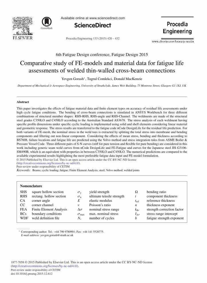
Appendix A. Summary of experiments and simulations
Summary of experiments and simulations including conditions and results of tests, analytical assessments andnumerical predictions is reported in Table A.3 for three variants of cross-beam connections: <1> tube (RHS) totube (RHS/SHS), <2> angle (CA) to tube (RHS/SHS), and <3> channel (CC) to tube (RHS/SHS). Comparison offatigue life predictions obtained with shell and solid FE-models with each other and experimental data is reported inTable A.4 for cross-beam connections with bottom member 50x50x3 SHS welded to three variants of top members:<1> 75x50x3 RHS, <2> 75x75x4 CA, and <3> 100x50x4 CC.
References
[1] P. Heyes, Fatigue analysis of seam welded structures using nCode DesignLife, Whitepaper, HBM nCode, Rotherham, UK, (Mar. 2013).URL:http://www.ncode.com/fileadmin/mediapool/nCode/downloads/DesignLife/Whitepaper_SeamWelds_nCodeDesignLife_201303-3.pdf.
[2] W. H. Munse, Fatigue of weldments – Tests, design, and service, in: D. W. Hoeppner (Ed.), Fatigue Testing of Weldments (ASTM STP 648),American Society for Testing and Materials, Philadelphia, PA, USA, 1978, pp. 89–112. DOI: 10.1520/STP648-EB.
[3] J. J. F. Bonnen, H. Agrawal, M. A. Amaya, R. M. Iyengar, H. T. Kang, A. K. Khosrovaneh, T. M. Link, H.-C. Shih, M. Walp, B. Yan, Fatigueof advanced high strength steel spot-welds, SAE Technical Paper no. 2006-01-0978 (2006) 1–20. DOI: 10.4271/2006-01-0978.
[4] N.-J. Ho, F. V. Lawrence Jr., C. J. Altstetter, The fatigue resistance of plasma and oxygen cut steel, Welding Research Supplement (Nov. 1981)231–236. URL: https://app.aws.org/wj/supplement/WJ_1981_11_s231.pdf.
[5] T. Palmer, Fatigue in welded-steel structures, Machine Design (Mar. 3, 2014). URL: http://machinedesign.com/metals/fatigue-welded-steel-structures.
[6] K.-H. Chang, Fatigue and fracture analysis, in: Product Performance Evaluation with CAD/CAE, The Computer Aided Engineering DesignSeries, Academic Press, Boston, USA, 2013, pp. 205–273. DOI: 10.1016/B978-0-12-398460-9.00004-4.
[7] P. Newbold, DesignLife Theory Guide, Version 9 ed., HBM nCode, Rotherham, UK, 2013.[8] F. R. Mashiri, X. L. Zhao, Welded thin-walled rhs-to-rhs cross-beams under cyclic bending, in: J. A. Packer, S. Willibald (Eds.), Proc. Tubular
Structures XI (Québec, Canada, 31 Aug. - 2 Sep. 2006), Taylor & Francis Group, CRC Press, London, UK, 2006, pp. 97–104.[9] F. R. Mashiri, X. L. Zhao, Thin RHS-Channel welded cross-beams under cyclic bending, in: J. Y. R. Liew, Y. S. Choo (Eds.), Proc. 5th Int.
Conf. in Advances in Steel Structures – ICASS 2007 (Singapore, 5-7 Dec. 2007), Research Publishing Service, Singapore, 2007, pp. 991–996.[10] F. R. Mashiri, X. L. Zhao, Tests of welded cross-beams under fatigue loading, in: Z. Y. Shen, Y. Y. Chen, X.-Z. Zhao (Eds.), Proc. Tubular
Structures XII (Shanghai, China, 8-10 Oct. 2008), Taylor & Francis Group, CRC Press, Boca Raton, FL, USA, 2008, pp. 163–170.[11] F. R. Mashiri, X. L. Zhao, Fatigue tests and design of welded thin-walled RHS-RHS and RHS-angle cross-beam connections under cyclic
bending, Thin-Walled Structures 48 (2010) 159–168. DOI: 10.1016/j.tws.2009.07.006.[12] F. R. Mashiri, X. L. Zhao, L. W. Tong, Fatigue tests and design of welded thin-walled RHS-Channel and Channel-Channel cross-beam
connections under cyclic bending, Thin-Walled Structures 63 (2013) 27–36. DOI: 10.1016/j.tws.2012.09.002.[13] Data Sheet on Fatigue Properties of Non-Load-Carrying Cruciform Welded Joints of SM490B Rolled Steel for Welded Structure, NIMS Fatigue
Data Sheets No. 91, 96, 99, 108, 114, National Institute for Materials Science, Tsukuba, Japan, (2003, 2004, 2006, 2009, 2011).[14] M. Fermér, M. Andréasson, B. Frodin, Fatigue life prediction of mag-welded thin-sheet structures, SAE Technical Papers (1998) 1–9.
DOI: 10.4271/982311.[15] A. Boiler, P. V. C. on Pressure Vessels, 2010 ASME Boiler & Pressure Vessel Code: Section VIII Division 2 – Alternative Rules, 2010 ed.,
ASME, New York, USA, 2010.[16] E. Haibach, FKM-Guideline: Analytical Strength Assessment of Components in Mechanical Engineering, 5th ed., VDMA Verlag, FKM,
Frankfurt am Main, Germany, 2003.[17] British Standard, Guide to fatigue design and assessment of steel products, BS 7608:2014, The British Standards Institution, London, UK,
2014.[18] R. G. Budynas, J. K. Nisbett, Shigley’s Mechanical Engineering Design, 9th ed., McGraw-Hill, New York, USA, 2010.[19] Australian / New Zealand Standard, Cold-formed structural steel hollow sections, AS/NZS 1163:2009, Standards Australia / Standards New
Zealand, Sydney /Wellington, 2009.[20] AustubeMills, TS100 – angles, channels, flats, DuraGal Technical Specifications, 7th ed., Australian Tube Mills Pty Ltd., Acacia Ridge,
QLD, Australia, 2013.[21] X.-L. Zhao, S. Herion, J. A. Packer, R. S. Puhtli, G. Sedlacek, J. Wardenier, K. Weynand, A. M. van Wingerde, N. F. Yeomans, Design guide
for circular and rectangular hollow section welded joints under fatigue loading, TÜV-Verlag GmbH, Köln, Germany, 2001.[22] J. Mentley, nCode DesignLife Weldline ACT Extension, PowerPoint Presentation, HBM - nCode Products (Southfield, MI, USA), 2015.
432
Yevg
en G
ora
sh et a
l. / Pro
cedia
Engin
eering 1
33 ( 2
015 ) 4
20 –
432
Table A.3. Summary of experiments and simulations including conditions and results of tests, analytical assessments and numerical predictions
No. Top Bottom ȴʍnom N* Failure ʍmax w (mm) N* ȴ, % N* ȴ, % N* ȴ, %
S1R1L1A 871688 6.184E+05 40.96 3.747E+05 132.64 8.479E+05 2.81
S1R1L2A 461734 6.184E+05 -33.93 3.747E+05 23.23 8.479E+05 -83.63
S2R1L1A 93.5 2304714 103.889 0.63081 1.319E+06 74.73 7.208E+05 219.74 1.942E+06 18.68
S2R1L2A 124.6 211506 138.444 0.84063 3.362E+05 -58.96 3.046E+05 -44.01 6.522E+05 -208.36
S4R1L1A 214.4 156087 238.222 2.06641 5.120E+04 204.86 8.373E+04 86.42 1.307E+05 19.42
S4R1L2A 193.0 179735 214.444 1.86015 8.448E+04 112.75 1.148E+05 56.56 1.949E+05 -8.44
S5R1L1A 35x35x1.6 SHS 135.0 1316243 150 1.30114 9.348E+04 1308.05 1.030E+05 1177.91 1.653E+05 696.28
R2R1L1A 65.2 7738790 no crack 72.444 0.43988 4.630E+06 under 2.047E+07 over
R2R1L2A 130.5 235219 145 0.88044 1.228E+06 -422.07 5.772E+05 -145.39 1.466E+06 -523.25
R3R1L1A 50x25x1.6 RHS 103.8 675844 115.333 0.7003 1.198E+06 -77.26 5.139E+05 31.51 1.265E+06 -87.17
-158.91 360.70 -869.95
S1AN1L1A 50x50x3 SHS 145.2 540340 161.333 0.91777 8.190E+05 -51.57 4.605E+05 17.34 1.128E+06 -108.76
S1AN1L2A 50x50x1.6 SHS 152.9 381510 169.889 0.96644 2.228E+05 71.23 2.002E+05 90.56 3.924E+05 -2.85
S4AN1L2A 35x35x3 SHS 87.6 3693392 97.333 0.791 3.380E+06 9.27 1.101E+06 235.46 3.347E+06 10.35
S5AN1L1A 35x35x1.6 SHS 110.3 775613 122.556 0.99597 6.222E+05 24.66 3.452E+05 124.69 7.642E+05 1.49
R2AN1L1A 50x25x3 RHS 133.2 403180 148 0.84192 8.329E+05 -106.58 4.520E+05 -12.11 1.075E+06 -166.63
R3AN1L1A 50x25x1.6 RHS 106.0 1371361 117.778 0.67 1.153E+06 18.94 5.103E+05 168.74 1.272E+06 7.81
-34.05 624.67 -258.59
S1C1L1A 353652 1.784E+05 98.24 1.791E+05 97.46 3.433E+05 3.02
S1C1L2A 611060 1.784E+05 242.52 1.791E+05 241.18 3.433E+05 78.00
S2C1L1A 50x50x1.6 SHS 96.5 255855 107.222 0.65105 4.854E+05 -89.72 3.707E+05 -44.89 9.638E+05 -276.70
S4C1L1A 177.2 265871 196.889 1.70787 1.098E+05 142.14 1.261E+05 110.84 2.136E+05 24.47
S4C1L2A 88.6 3760725 98.444 0.85394 2.980E+06 26.20 1.009E+06 272.72 2.973E+06 26.50
S5C1L1A 35x35x1.6 SHS 139.5 990477 155 1.34451 2.607E+05 279.93 1.966E+05 403.80 3.747E+05 164.34
R2C1L1A 50x25x3 RHS 134.8 146712 149.778 0.90945 3.262E+05 -122.34 2.530E+05 -72.45 5.156E+05 -251.44
R3C1L1A 50x25x1.6 RHS 107.2 2711681 119.111 0.72324 9.561E+05 183.62 4.540E+05 497.29 1.081E+06 150.85
760.59 1505.96 -80.97
25.80 113.24 -54.98Total discrepancy for all considered experiments:
75
x5
0x3
RH
S7
5x7
5x4
CA
10
0x5
0x4
CC
Gro
up
sT
ub
e t
o t
ub
eC
orn
er
to t
ub
eC
ha
nn
el
to t
ub
e
bo
tto
m m
em
be
r
BM
bo
tto
m m
em
be
rb
ott
om
me
mb
er
Analytical
assessments
Experimental data for cross-beam connections with different
combinations of beam profiles
Total discrepancy for the above group of tests:
Total discrepancy for the above group of tests:
166.333 1.00998
SM490B steel welds generic S-N curve DL generic S-N curve FEF
Numerical predictions with nCode DesignLife
50x50x1.6 SHS
35x35x3 SHS
50x50x3 SHS 149.7
50x25x3 RHSno crack estimated
Total discrepancy for the above group of tests:
1.04371
35x35x3 SHS
50x50x3 SHS 154.7 171.889
Table A.4. Comparison of fatigue life predictions obtained with shell and solid FE-models with each other and experimental data
1 2 3 total
No. Top member N* N* ȴ, % N* ȴ, % N* ȴ, % N* ȴ, % N* ȴ, % N* ȴ, % ȴ, % ȴ, % ȴ, % ȴ, %
S1R1L1A 871688 41.0 107.2 132.6 192.7 2.8 36.5
S1R1L2A 461734 -33.9 9.7 23.2 55.0 -83.6 -38.3
2 S1AN1L1A 75x75x4 CA 540340 8.190E+05 -51.6 7.175E+05 -32.8 4.605E+05 17.3 4.116E+05 31.3 1.128E+06 -108.8 9.549E+05 -76.7 14.1 11.9 18.1 14.7
S1C1L1A 353652 98.2 148.4 97.5 124.8 3.0 20.6
S1C1L2A 611060 242.5 329.1 241.2 288.5 78.0 108.4
6.184E+05
1.784E+05
3.747E+05
1.791E+05
8.479E+05
3.433E+05
Experiments for connection with
bottom member 50x50x3 SHS
75x50x3 RHS
100x50x4 CC
Case
No.
1
3
difference - shell vs. solid
18.71.424E+05 1.573E+05
32.8 35.24.208E+05 2.978E+05 6.386E+05 47.0 25.8
2.932E+05 25.3 13.9 17.1
SM490B steel welds 1 generic S-N curve DL 2 generic S-N curve FEF 3
shell FEs solid FEs shell FEs solid FEs shell FEs solid FEs
Related Documents