Stopover strategies in passerine bird migration: a simulation study

J. theor. Biol. (2002) 219, 479–493doi:10.1006/yjtbi.3138, available online at http://www.idealibrary.com on

Stopover Strategies in Passerine Bird Migration: A Simulation Study

Birgit Erninw, Felix Liechtiw and Bruno Brudererw

wSwiss Ornithological Institute, CH-6204 Sempach, Switzerland

(Received on 19 December 2001, Accepted in revised form on 9 July 2002)

Long-distance bird migration consists of a series of stopovers (for refuelling) and flights, withflights taking little time compared to stopovers. Therefore, it has been hypothesized that birdsminimize the total time taken for migration through efficient stopover behaviour. Currentoptimality models for stopover include (1) the fixed expectation rule and (2) the global updaterule. These rules maximize the speed of migration by determining the optimal departure fuelload for a given fuel deposition rate. We were interested in simple behavioural rulesapproaching the stopover behaviour of real birds and how these rules compare to the timeminimizing models above with respect to the total time taken for migration. The simplestrategies were to stay at a site (1) until a fixed fuel load was reached or (2) for a constantnumber of days. We simulated migration of small nocturnal passerine birds across anenvironment of continuously distributed but variable fuel deposition rates, and investigatedthe influence of different stopover strategies on the duration of migration. Staying for aconstant number of days at each stopover site, irrespective of the fuel deposition rate,resulted in only slightly longer than minimum values for migration duration. Additionally,the constant stopover duration, e.g. 10 days, may change by a day or two (per stopover)without having a large effect on total migration duration. There is therefore a possibility thatreal birds may be close to optimal migration speed without the need for very complexbehaviour. When assessing the sensitivity of migration duration to factors other thanstopover duration, we found that flight costs, search and settling time, mean fuel depositionrate and the accuracy in the choice of flight direction were the factors with the largestinfluence. Our results suggest that migrating birds can approximate optimal stopoverduration relatively easy with a simple rule, and that other factors, e.g. those above, are morerelevant for travel time.

r 2002 Elsevier Science Ltd. All rights reserved.

Introduction

To be at the right place at the right time is thesecret of successful migration. The proper timingof resting and moving is an indispensableprerequisite, especially for long-distance mi-grants (Alerstam & Lindstrom, 1990). Long-distance migration in passerine birds is mostlyruled by a series of stopovers of a few days

nCorresponding author.E-mail address: [email protected] (B. Erni).

0022-5193/02/$35.00/0

interrupted by migratory flights that, comparedto stopover duration, take very little time(Hedenstrom & Alerstam, 1997). The total timetaken for migration is therefore strongly influ-enced by how efficiently a migrating bird can useavailable stopover sites for refuelling. Alerstam& Lindstrom (1990) first developed modelswhich predict the stopover duration at agiven site when optimizing energy or time.Time optimizing stopover models are built onassumptions that birds either minimize time

r 2002 Elsevier Science Ltd. All rights reserved.

B. ERNI ET AL.480

based on an expectation of conditions ahead, thefixed expectation rule (Alerstam & Lindstrom,1990; Weber & Houston, 1997a; Houston, 1998),or based on the currently experienced fueldeposition rate, the global update rule (Houston,1998; Weber, 1999; Weber et al., 1999). Data didnot support the hypothesis that birds minimizetime based on a fixed expectation of refuellingrates (Lindstrom & Alerstam, 1992; Weber et al.,1999). Possible explanations for this discrepancyinclude the costs of large fuel loads (Klaassen &Lindstrom, 1996), the influence of wind condi-tions on the departure decision (Weber &Hedenstrom, 2000) and the poor performanceof this strategy with spatially autocorrelated fueldeposition rates (Weber, 1999). Weber (1999)and Weber et al. (1999) suggested that birds mayinterpret the current fuel deposition rate as anindication of future conditions and minimizetime based on this assumption (global updaterule).

In this study, we investigate stopover beha-viour of passerine migrants with the aid of acomputer simulation. What are the conse-quences on the total time taken for migrationwhen stopover rules and stopover conditionschange? Are there simple rules of thumb that canapproach the time minima of optimal stopover?With emphasis on simulating a realistic situationfor passerine migration, we compare timeoptimizing stopover models with two simplerstopover rules, simpler in that no knowledgeabout the environment ahead is required orextrapolated from experienced values, and theyare not explicitly intended to minimize time. Weconsider the following two simple strategies: (1)a stopover site is used until a threshold fuel levelis reached and (2) a stopover site is used for aconstant number of days. We investigate howthese two strategies compare to the followingmodels on stopover strategy (Alerstam &Lindstrom, 1990; Houston, 1998): (3) the fixedexpectation rule, where time is minimized basedon a fixed expectation of conditions ahead and(4) the global update rule, where encounteredfuel deposition rates are interpreted as represen-tative of conditions ahead and time is optimizedwith respect to this assumption. The latter twostrategies can be further optimized if theremaining distance is known (Weber & Houston,

1997a; Weber, 1999). Thus, we compare fourmodels based on different optimality criteria andtwo ‘‘simple rules’’ models (Appendix A).

This study is aimed primarily at nocturnallong-distance migration of inexperienced passer-ines on their first autumn journey, taking thegarden warbler Sylvia borin as a typical example.In the first part, stopover strategies are com-pared under different refuelling conditions. Forthis a linear simulation is used, i.e. stopover siteswere distributed along a straight line (similar toWeber, 1999). In the second part, the sensitivityof migration duration to a number of factors(mean and variation in fuel deposition rates,flight costs, orientational error, search andsettling time, stopover duration) is analysed.For this a two-dimensional grid of cells is used tomodel the environment.

This study (comparison of stopover strategies)is the first part of a larger simulation model ofpasserine bird migration. Other important en-vironmental factors such as wind, rain andtopography (Alerstam, 1976; Erni et al., 2002)will be analysed in forthcoming studies. Ourultimate aim is a tool to investigate and testhypotheses of passerine migration. For this it isnecessary to first obtain a thorough under-standing of the influence of stopover behaviouron total migration time.

Methods

The environment was modelled in two ways:(a) in the first part, for the comparison ofstopover strategies, as a continuous line, with thefuel deposition rate changing every 4 km, and (b)as a two-dimensional grid of 100 km� 100 kmcells for the sensitivity analyses in the secondpart, with a different fuel depostion rate for eachcell. Fuel deposition rates (FDRs) were ran-domly assigned from a uniform distribution withvalues between e.g. 0.0570.04 (mean7d), whered is a measure of the variability of the FDRs.FDR k is expressed as the daily gain in massrelative to lean body mass, with unit per day(Alerstam & Lindstrom, 1990). Spatially auto-correlated FDRs were formed similar to Weber(1999), as a moving average process [eqn (1)].Here the ei’s (assigned to each cell i) areuniformly distributed random variables with

STOPOVER STRATEGIES IN BIRD MIGRATION 481

mean zero and range such that the resultingrange of ki is approximately 0.08 (7d) accordingto the distribution of the sum of randomvariables (Rice, 1988). We looked at autocorre-lations over distances of 40, 120 and 200 km andfor these the ranges for the ei’s were 0.367, 0.625and 0.802, respectively. The weights ws decreasewith increasing distance s between cells, smeasured in number of cells [eqn (2)].

ki ¼ %k þXq

s¼�q

wsei�s

!,Xq

s¼�q

ws; ð1Þ

ws ¼ expð�as2Þ; ð2Þ

where ki is the FDR in cell i, %k is the overallmean FDR ¼ 0.05, a determines how fast theweights decrease and was set to 0.0001 (slowdecrease), q is the number of cells over which theautocorrelation stretches to either side and isincreased to increase the spatial autocorrelation.We assigned values of 10, 30 and 50 to q. Withcells of size 4 km this means that FDRs wereautocorrelated over distances of 40, 120 and200 km, respectively. Resulting FDRs were thenroughly distributed between 0.01 and 0.09 withmean 0.05. FDRs that fell beyond the limitsof 0.09 or 0.01 were redistributed uniformlybetween 0.08 and 0.09 or 0.01 and 0.02,respectively.

Birds were defined in terms of behaviouralrules (e.g. stopover strategy, flight time pernight) and their state (e.g. fuel level, position).We neglected energy loss during non-flightphases. The flight range Y with a given fuel loadx (x ¼ kt, where t is the stopover durationexcluding search and settling time) was calcu-lated as in Alerstam & Lindstrom (1990):

Y ðxÞ ¼ c 1 �1ffiffiffiffiffiffiffiffiffiffiffi

1þ xp

!ð3Þ

with a flight range constant c of 8500 km(estimate for a bluethroat, Lindstrom & Aler-stam, 1992). This constant depends on physicaland aerodynamic values (Pennycuick, 1989;Alerstam & Hedenstrom, 1998) for many ofwhich approximate values are still estimatedwith much uncertainty (Piersma & Jukema,

1990; Biebach, 1992; Pennycuick et al., 1996;Hedenstrom & Weber, 1999). c was included as afactor in the sensitivity analyses. When reachinga new stopover site after a flight stage, the initialgain in body mass sometimes is low (e.g.Klaassen & Biebach, 1994). This was modelledas a time cost (in days) during which birds didnot deposit fuel: the search and settling time(SST).

STOPOVER STRATEGIES

Detailed descriptions of theoretical stopoverstrategies can be found in Alerstam & Lindstrom(1990), Weber & Houston (1997a), Alerstam &Hedenstrom (1998), Houston (1998) and Weber(1999). A summary of the stopover strategiescompared here and abbreviations used are givenin Appendix A.

Fixed expectation rule (FE1): Birds are as-sumed to have a fixed expectation of the FDRson the route ahead. The birds also assume thatencountered deviations from this expectation aredue to local variation (Houston, 1998). Theinstantaneous speed of migration (or the margin-al rate of gain in potential flight range) is

dY

dt¼

ck

2ð1 þ ktÞ�3=2; ð4Þ

where Y is the flight range and c is the flightrange constant [eqn (3)]; k is the current FDRand t is the stopover duration excluding SST. Tominimize time, a bird should leave the currentsite when the instantaneous speed of migrationdrops to the expected speed of migration(marginal value theorem, Charnov, 1976; Aler-stam & Lindstrom, 1990). The expected speedis found by substituting for k the expected (wetook the mean) FDR (kexp) and for kt theoptimal departure fuel load at kexp. The optimaldeparture fuel load (or equivalently the optimalstopover duration) is found numerically fromeqn (6).

Fixed expectation rule with known remainingdistance (FE2): As in FE1 birds have a fixedexpectation of conditions ahead. Weber &Houston (1997a) stated that when the totaldistance is finite, the marginal value theorem [asimplemented in eqn (4)] no longer minimizestime. We will refer to finite distance as known

B. ERNI ET AL.482

remaining distance, similarly as unknown re-maining distance instead of infinite distance.When minimizing time under this additionalcondition, the remaining (known) distance isdivided into steps of equal length (Weber &Houston, 1997a) because the expectation for theremaining distance is constant. We look at theoutcomes with this additional assumption,although for passerine migrants an unknownremaining distance would be more typical(Weber & Houston, 1997a).

Stopover sites were evenly distributed at 4 kmintervals following Weber (1999). The target sitem is that for which the total remaining time isminimized (current stopover time plus remainingtime tm to end). The remaining time tm (timefrom reaching target site m to end) is found as inGU2 [eqn (7)] by substituting for k the expectedFDR and dividing the remaining distance intoan optimal number of steps nn. Then the targetsite m is found numerically [eqn (5)] as that whichminimizes current stopover duration plus remain-ing time tm [eqn (8) in Weber & Houston, 1997a].M is the total number of sites (1000in our simulation), D is the total distance(4000km), m is the target site and i is the currentsite. ki is the FDR at the current site, te is the SST:

minm

1

ki

c2

ðc � ððm � iÞD=MÞÞ2� 1

!þ te þ tm

!;

iompM: ð5Þ

Global update rule (GU1): The FDR at the currentsite is interpreted as representing the global(future) habitat quality (Houston, 1998). Theoptimal stopover time tn is found numerically bymaximizing the speed of migration:

maxt

Y

t¼

c�1 � ð1 þ kðt � teÞÞ

�0:5�

t

!; ð6Þ

where t is the total stopover time at the currentsite, including SST te. Only integer values fort were considered. The optimal departure fuel loadthen is kðtn � teÞ: For both FE1 and GU1 [eqns(4) and (6)], the optimal stopover duration doesnot change when the flight range constantc changes. Speed of migration is however still

maximized at the same stopover duration and willincrease with increasing c.

Global update rule with known remainingdistance (GU2): As in GU1, the FDR furtheralong the route is assumed to equal the currentFDR. The remaining distance is divided into anequal number of steps. The optimal departurefuel load is enough only to reach the next site.The optimal number of steps, nn, minimizes theremaining time T(n) [Weber & Houston, 1997a,eqn (4)], nn has to be found numerically bysubstituting integer values for n in eqn (7). Dr isthe remaining distance, te is the SST, c is theflight range constant:

TðnÞ ¼ n1

k

c2

ðc � Dr=nÞ2� 1

!þ te

!: ð7Þ

Having solved for nn, the optimal stopoverduration is found by substituting Dr/n

n for Y(the length of one step) in eqn (6). Stopover sitesare, as in FE2, assumed to be evenly distributedat 4 km intervals, D¼ 4000 km. In FE2 andGU2, the optimal stopover duration dependsboth on the current FDR and on the value of c.These two strategies minimize the remainingtime by optimizing step lengths. Although theinstantaneous speed of migration is not max-imized, these two strategies will take less timethan FE1 and GU1 because at the last stopoversite departure fuel loads are enough only toreach the end, whereas in FE1 and GU1 fuelloads from the last stopover site will in mostcases be larger.

The simple stopover strategies areThreshold fuel load (TFL): The bird leaves a

site when, at the end of a day, its fuel level equalsor exceeds a certain threshold value, e.g. x ¼ 0:4(40% of lean body mass). This threshold level isindependent of the currently experienced FDR.A constant departure fuel load (TFL) is equiva-lent to using flight steps of equal length.

Constant stopover duration (CSD): The birdstays for a constant number of days independentof the current habitat quality.

The chosen default values for the latter twostrategies are a threshold fuel level of 0.4 and astopover duration of 10 days, respectively. Thesecorrespond to the optimal departure fuel load

STOPOVER STRATEGIES IN BIRD MIGRATION 483

and the optimal stopover duration with constantFDRs of 0.05 day�1 and an SST of 2 days [eqn(6)]. With no variation between FDRs, FE1,GU1, TFL and CSD are equivalent.

In the development of strategies FE1, FE2,GU1 and GU2, the flight time was assumednegligible compared to the stopover time (Aler-stam & Lindstrom, 1990), i.e. the flight rangewas assumed to be covered in a single flight ofone night. To model nocturnal passerine migra-tion representative of continental Europe, welimited the flight time per night to 8 h (Cochranet al., 1967; Zehnder et al., 2001). As aconsequence, birds with large fuel loads cannotcover the potential range in one flight but losedays during which they wait for the next nightto finish the flight stage. A new time optimumshould be calculated accounting for both, thetime spent refuelling and in flight (pointed out byAlerstam & Lindstrom, 1990), but this wouldincrease the complexity and reduce the applic-ability of the resulting solution. Therefore, withthe assumption of restricted flight time per nightwe use the optimal stopover models as approx-imations for maximum migration speeds. Wecompared these stopover strategies under chang-ing fuelling conditions by varying SST, meanFDR and variation in FDRs. Each situation wasreplicated 1000 times.

SENSITIVITY ANALYSES

To investigate the sensitivity of total migra-tion time to a number of factors, we looked attwo different reference situations and changedfactors by approximately 10% from their re-ference values. The environment was modelledas a two-dimensional grid of cells (a map of55� 65 cells), each cell was assigned an FDR asbefore. The cell size was 100 km� 100 km. Foreach combination of parameters the simulationwas repeated with 20 different maps, with 1000simulated birds for each map. The birds startedat a single point but chose different routes due toa standard error in choice of direction (meandirection 1801). The migration route was com-pleted when a horizontal line 4000 km due southof the starting point was crossed.

The following standard parameter settingswere used (reference situation A): fuel deposition

rates were distributed uniformly between0.0570.03 (mean7d ), SST was 2 days, theflight direction was chosen at the beginning ofeach night from a wrapped normal distributionwith mean and angular deviation 180 and 451(Liechti, 1992), respectively (corresponding toa mean vector length of r ¼ 0:692; Batschelet,1981), flight time per night was restricted to 8 hr,air speed was 10.5ms�1 (for small passerines,Biebach, 1992; Liechti & Bruderer, 1995). Thedefault stopover strategy was to stay for aconstant (CSD) 10 days at sites. The flight rangeconstant c was set to 8500 km (Lindstrom &Alerstam, 1992; Weber, 1999).

To investigate the influence of the sameparameters in a different situation (referencesituation B), we decreased c to 7000 km (i.e.increased flight costs), the mean FDR to 0.04(decreased habitat quality), SST to 1 day and theconstant stopover duration to 6 days. Fromthese two reference situations, the factors werechanged one at a time and the change in meantotal migration time was calculated. The changesmade were as follows: mean FDR 70.005,d70.006, SST71 day, stopover duration71day, c710%, angular deviation in flight direc-tion 751, mean flight direction +101. Finallythe stopover strategy was changed from CSD toFE1 and GU1.

Results

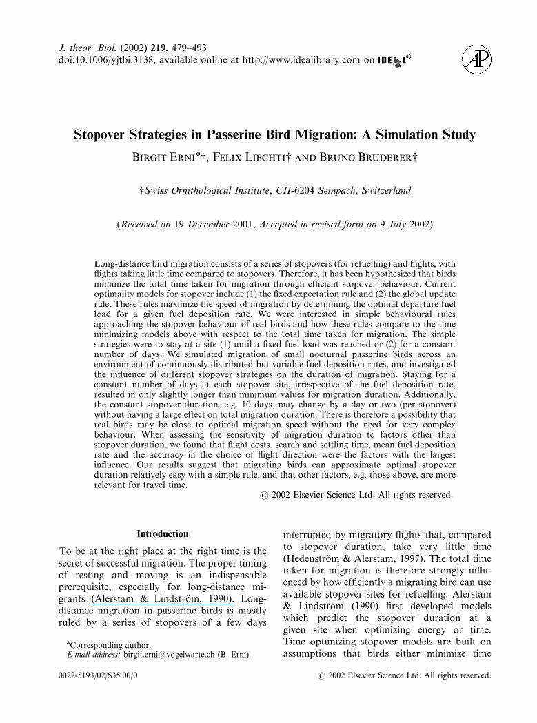
The effect of limiting flight time per night to8 hr, as opposed to assuming flight time to benegligible, was approximately equal for all stop-over rules (Fig. 1); a time increase of between10.4 and 12.1 days in the mean total migrationtime, e.g. the difference in mean total timebetween constant stopover duration (CSD) andthe fixed expectation rule (FE1), did not decrease[time difference: 2.1 days with unrestricted flighttime, 2.3 days with restricted flight time; unrest-ricted flight time: 35.176.1 days for FE1 (meantotal time7s.d.), 37.477.5 days for CSD;restricted flight time: 46.775.6 days for FE1,48.877.2 days for CSD]. We conclude from thisthat the relative optimality of FE1 over CSD wasnot affected by restricting flight time per night.All the following results were derived byrestricting flight time to 8 hr per night.

20

40

60

80

100

120

FE1 FE2 GU1 GU2 TFL CSD

tota

l m

igra

tion

tim

e (

days

)

Fig. 1. Total migration time for each of the six stopover strategies. Within each stopover strategy the four box-and-whisker plots show total migration time when fuel deposition rates were spatially autocorrelated over 0, 40, 120, 200 km.Boxes indicate the lower quartile, median and upper quartile, whiskers indicate minimum and maximum total migrationtime. Filled triangles show the mean total migration time. Circles represent the mean total migration time when flight timewas not restricted (i.e. assumed negligible) at no spatial autocorrelation between FDRs. SST 2 days, FDR 0.0570.04. ForFE2 at autocorrelations of 120 and 200 km, the upper quartiles were 128 and 188 days, respectively, maximum time was notcalculated. For TFL at autocorrelation 40 km the maximum time was 122 days.

B. ERNI ET AL.484

Spatial autocorrelation in FDRs affectedmainly FE1 and FE2 (Fig. 1). For FE2, themedian total migration time increased from 43 to50 days (at autocorrelations over distances of0 and 200 km, respectively), the arrival timedistributions were increasingly skewed to theright with increasing spatial autocorrelation. ForFE1, the mean time increased from 46.775.6 to50.278.8 days (median time increased from 47to 49 days) for an increase in spatial autocorre-lation from 0 to 200 km. In all other strategiesneither mean nor variance of time changed withincreasing spatial autocorrelation (Fig. 1). Thesimple rule models, TFL and CSD, did notperform worse than GU1 with autocorrelatedFDRs, although the variance in travel times withTFL was always larger. The difference betweenmean and median values in CSD is due to almostseparate peaked waves of arriving birds.

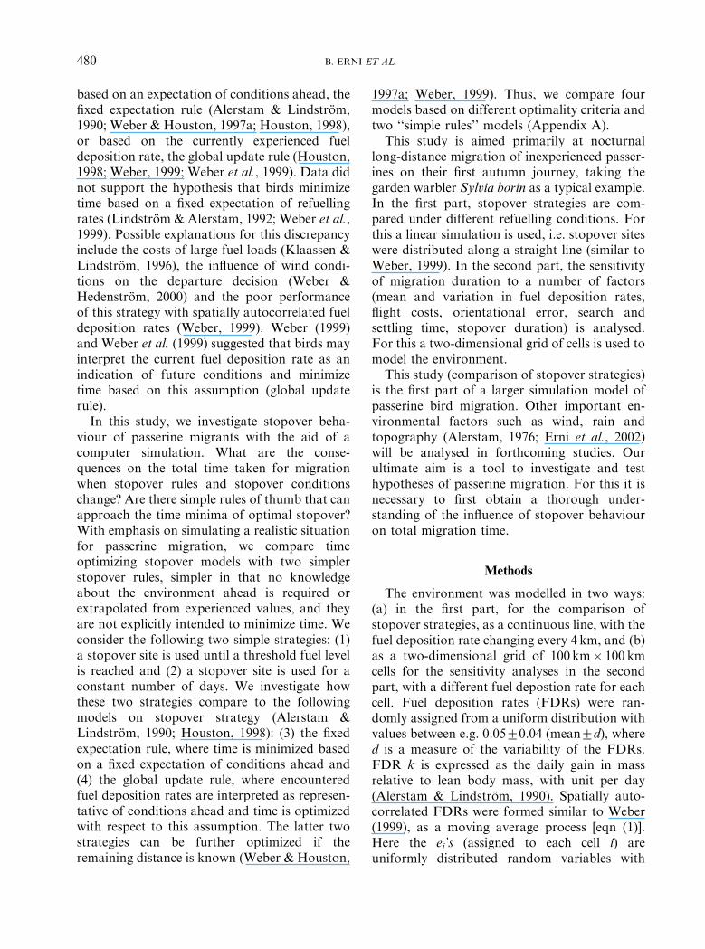
Figure 2 shows the influence of changingenvironmental conditions (FDR, SST) on thefour stopover strategies FE1, GU1, TFL andCSD. For TFL and CSD, the threshold fuel leveland the stopover duration, respectively, werevaried additionally. The general pattern in allfour stopover rules was an increase in totalmigration time with increasing SST and adecrease in total migration time with increasingmean FDRs. The changes in time caused by anincreasing variability in fuel deposition rates

were comparatively small [Figs 2(a–d)]. ForFE1, the largest increase in mean time from thestandard situation (mean FDR 0.0570.04, SST2 days) occurred with a decrease in mean FDRsto 0.03 day�1 [95% Confidence interval (CI) forincrease in mean time: 15.6, 16.7 days], and withan increase in SST to 4 days [9.1, 10.3 days]. Thelargest decrease occurred with an increase inmean FDR to 0.07 [�7.3, �6.5 days] and whenthe SST dropped to 1 day [�6.3, �5.5 days]. Thispattern was the same in GU1, TFL and CSD[Figs 2(b–d)]. With increasing variability (d) inFDRs, with FE1 mean time did not increase;however the standard deviation increased from3.5 to 6.1 days [Fig. 2(a)]. For GU1, thestandard deviation increased from 1.4 to 17.2days. There is some indication of a u-shapedtrend with increasing d [Figs 2(b–d)]. This mayhave been caused by an increased availability ofbetter stopover sites initially being of morebenefit than poor sites, but with a furtherincrease in FDR variability the influence of thepoor sites becomes stronger. This effect isstrongest for TFL [Fig. 2(c)], s.d. increasingfrom 2.2 to 49.7 days. With TFL and GU1 birdsspend too much time at poor stopover sites,because the mean overall FDR is not consideredin the decision of when to leave the site. ForCSD, the increase in the standard deviation wasfrom 4.8 to 9.1 days [Fig. 2(d)]. In summary, the

20

40

60

80

0.25 0.3

0.35 0.4

0.45 0 1 2 3 4

0.03

0.04

0.05

0.06

0.07 0

0.01

0.02

0.03

0.04

0.05

tota

l tim

e (d

ays)

(c) TFL

FDR SST d TFL

20

40

60

80

4 6 8 10 12 0 1 2 3 4

0.03

0.04

0.05

0.06

0.07 0

0.01

0.02

0.03

0.04

0.05

tota

l tim

e (d

ays)

(d) CSD

FDR SST d CSD

20

40

60

80

1 2 3 4

0.03

0.04

0.05

0.06

0.07 0

0.01

0.02

0.03

0.04

0.05

tota

l tim

e (d

ays)

(a) FE1

FDR SST d

20

40

60

80

1 2 3 4

0.03

0.04

0.05

0.06

0.07 0

0.01

0.02

0.03

0.04

0.05

tota

l tim

e (d

ays)

(b) GU1

FDR SST d

Fig. 2. Total migration time (mean7s.d.) for the stopover strategies: (a) fixed expectation rule, (b) global update rule,(c) threshold fuel level and (d) constant stopover duration. In each stopover strategy, SST, mean FDR and variability d inFDRs were varied (horizontal axis). For TFL and CSD, the threshold departure fuel level and stopover duration (days),respectively, were varied additionally. With changing SST, FDRs were distributed between 0.0570.04, else SST¼ 2. Withchanging mean FDR, d ¼ 0:02; with changing d, mean FDR¼ 0.05

STOPOVER STRATEGIES IN BIRD MIGRATION 485

implications for migration are that with adecrease in mean FDR of 0.01 (from 0.05 to0.04) the total migration time would increase byca. 5–6 days. With a further drop of 0.01 to amean of 0.03, total migration time wouldincrease by another 9–10 days. With increasingvariation in FDRs the variance of arrival timeswould increase but this depends on the stopoverrule and the increase is smallest when stopoverduration depends also on the mean overall FDR(FE1).

Total migration time changed irregularlywhen threshold fuel levels were increased[Fig. 2(c)]. This pattern was constant when theruns were repeated under the same parametersettings and may have been caused by acombination of the following two factors: (a)how efficiently the total distance of 4000 km canbe covered with a given threshold fuel level and(b) how efficiently the potential flight range (witha given fuel load) can be covered in consecutiveflight nights. Changing stopover duration inCSD had little influence on time, only with shortand long stopover durations did migration timeincrease [stopover durations 4 and 12 days,

Fig. 2(d)]. At FDR¼ 0.0570.04 and SST 2 days,the difference in total migration times between aCSD of 6, 8 or 10 days was at most 2 days.

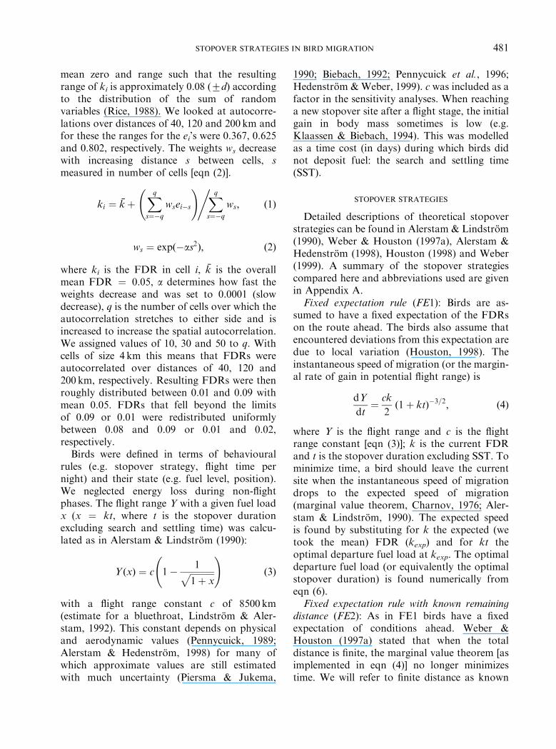
We calculated the time differences betweenFE1 vs. FE2 and GU1 vs. GU2 under differentstopover conditions (Fig. 3). In FE1 vs. FE2, thetime differences ranged between 1.4 (SST ¼ 1day) and 7.0 days (d ¼ 0) but otherwise wereapproximately constant between 3 and 5 days(average difference 4.2 days). With no variationin the FDRs (d ¼ 0), FE2 can calculate theoptimal step length without error. With increas-ing FDR variability, the extrapolated FDR usedby GU2 more often does not correspond to themean FDR [Fig. 3(b)]. This results in moreerrors in the calculated step lengths and hencethe migration times become more similar tothose of GU1. Stopover duration increases withincreasing SST [eqn (6)], resulting in largerdeparture fuel loads and therefore longer steps.With longer steps the probability that the laststep will not fit exactly into the remainingdistance increases, causing larger time differ-ences between the models with unknown vs.known remaining distance [Figs 3(a) and (b)].

-2

0

2

4

6

8

10

1 2 3 4

0.03

0.04

0.05

0.06

0.07 0

0.01

0.02

0.03

0.04

0.05

time

diffe

renc

e (d

ays)

FE1 - FE2

SST d FDR

-2

0

2

4

6

8

10

1 2 3 4

0.03

0.04

0.05

0.06

0.07 0

0.01

0.02

0.03

0.04

0.05

time

diffe

renc

e (d

ays)

GU1 - GU2

SST d FDR

(a)

(b)

Fig. 3. Time differences between (a) FE1 and FE2 (timedifference calculated as FE1�FE2) and (b) GU1 and GU2(time difference calculated as GU1–GU2). Error bars showthe 95% CI limits for the difference in mean times of thetwo strategies being compared. The time differences werecalculated for each condition indicated on the x-axis. Withchanging SST, FDRs were uniformly distributed between0.0570.04, else SST¼ 2. With changing mean FDR, d ¼0:02; with changing d, mean FDR¼ 0.05.

B. ERNI ET AL.486

Depending on the total migration distance, flighttime per night and the distribution of FDRs, thedifference in total migraton time between thetwo strategies (distance known vs. unknown)will vary, but will never exceed the duration ofone stopover (of FE1 or GU1). For absolutemigration times (FE1 and GU1) see Figs 2(a)and (b).

The assumption of known remaining distanceis unlikely and in some situations produces poorresults (FE2 in Fig. 1). We therefore did notconsider FE2 and GU2 any further.

COMPARISON OF STOPOVER STRATEGIES

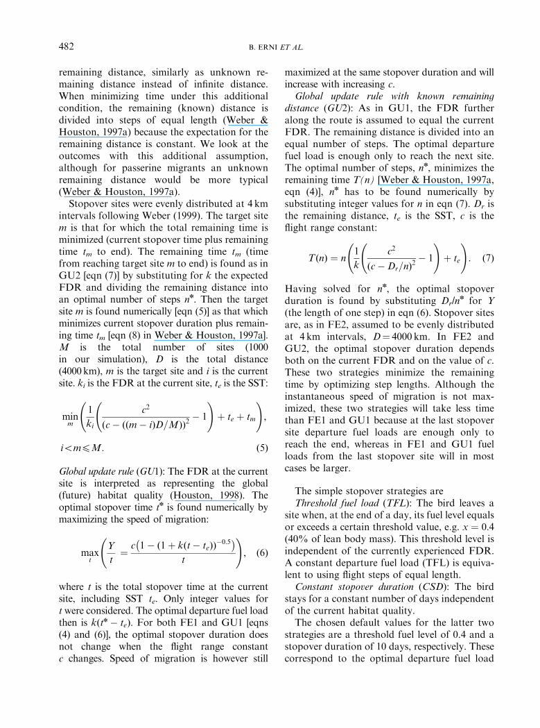
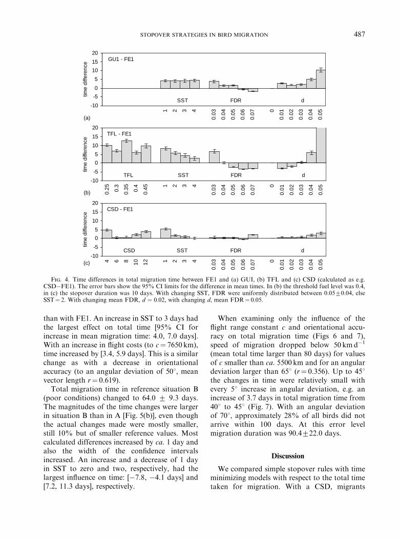
Under the same stopover conditions as above,we compared stopover strategies GU1, TFL andCSD with FE1 [Figs 4(a–c), see Figs 2(a–d) forthe absolute times]. These comparisons give anidea of the difference in total migration timebetween simple stopover rules and the totalmigration time when birds would stopover for

the theoretically optimal duration. The differ-ences between GU1 and FE1 were small[Fig. 4(a)]. The average time difference over allsituations was 2.9 days and only exceeded 5 dayswith large FDR variability [95% CI for differ-ence in mean total migration time: 5.2, 7.2 days].With no variation in FDRs all four strategieswere equivalent. TFL took less time than FE1with large mean fuel deposition rates and smallFDR variability but in all other situations tooklonger than FE1 [Fig. 4(b)]. The time differencewas largest for small SSTs [7.5, 9.2 days] and fora large FDR variability [25.8, 32.0 days]. Forsmall FDRs and large SSTs, i.e. poor environ-mental conditions, the time differences weresmall [Fig. 4(b)]. With different threshold fuellevels the time differences varied but were alwayspositive, i.e. TFL always took more time. With aconstant stopover duration (CSD) of 10 days thetotal migration time at different situationsclosely resembled (difference o 1 day) those ofFE1 except with small SSTs (1 and 2 days),d¼ 0.04 and 0.05 and a mean FDR of 0.07[Fig. 4(c)]. With a small SST, a shorter constantstopover duration would be more appropriatethan the 10 days used here. With a mean FDR of0.07 the time difference was [1.8, 2.2 days] andwith d ¼ 0:05 [2.2, 3.5 days] [Fig. 4(c)]. The timedifferences were smaller than between GU1 andFE1 [Fig. 4(a)]. With shorter stopover durationsthan 10 days (6 or 8 days), the difference in totalmigration time compared to that of FE1decreased.

SENSITIVITY ANALYSES

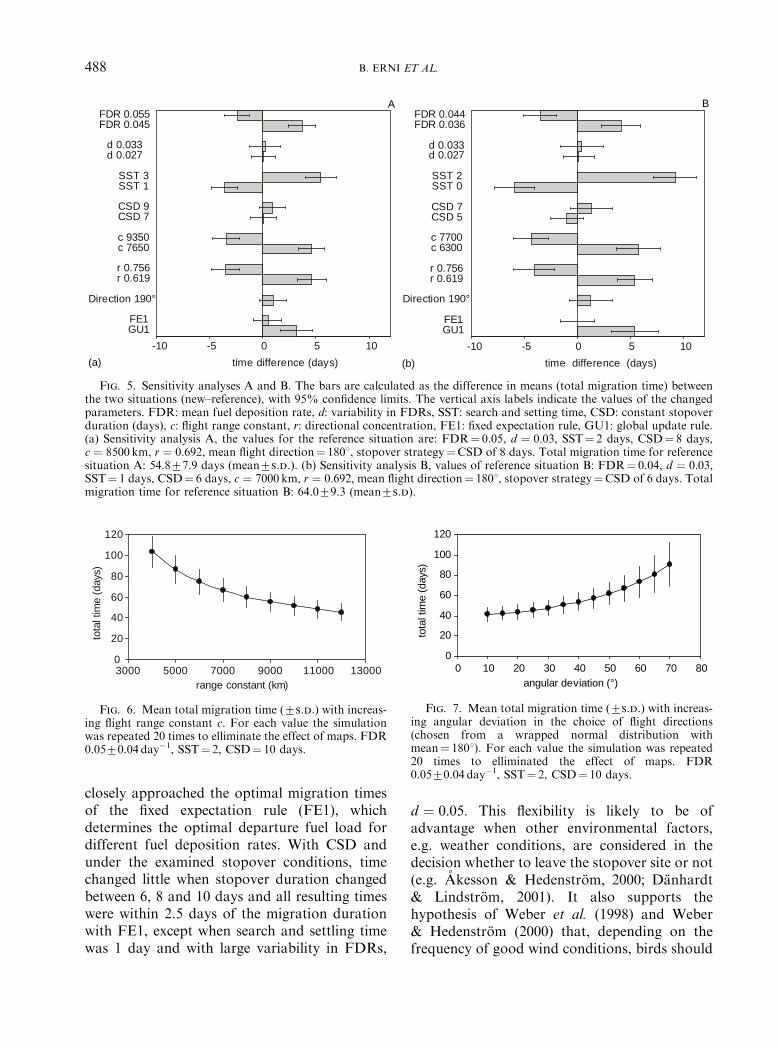
The change from a linear simulation to a two-dimensional environment caused an increase intotal migration time from 48.877.1 (mean7s.d.)to 54.877.9 days and total distance flownincreased from 4000 km to 54707564 km[Fig. 5(a)]. An increase or decrease of 1 day instopover duration, a change of 101 in mean flightdirection to 1901, a change of 10% in d and usingFE1 as stopover strategy instead of CSD[Fig. 5(a)] had little influence on total migrationtime (less than 1 day). With a stopover durationof 8 days, birds need slightly less time than withFE1, but when the constant stopover durationwould increase to 9 days, they would need longer

-10

-5

0

5

10

15

20

1 2 3 4

0.0

3

0.0

4

0.0

5

0.0

6

0.0

7 0

0.0

1

0.0

2

0.0

3

0.0

4

0.0

5

time

diffe

renc

e

GU1 - FE1

FDR d SST

-10

-5

0

5

10

15

20

0.2

5

0.3

0.3

5

0.4

0.4

5 1 2 3 4

0.0

3

0.0

4

0.0

5

0.0

6

0.0

7 0

0.0

1

0.0

2

0.0

3

0.0

4

0.0

5

time

diffe

renc

e

TFL - FE1

FDR d SST TFL

-10

-5

0

5

10

15

20

4 6 8 10

12 1 2 3 4

0.0

3

0.0

4

0.0

5

0.0

6

0.0

7 0

0.0

1

0.0

2

0.0

3

0.0

4

0.0

5

time

diffe

renc

e

CSD - FE1

FDR d SST CSD

(a)

(b)

(c)

Fig. 4. Time differences in total migration time between FE1 and (a) GUI, (b) TFL and (c) CSD (calculated as e.g.CSD�FE1). The error bars show the 95% CI limits for the difference in mean times. In (b) the threshold fuel level was 0.4,in (c) the stopover duration was 10 days. With changing SST, FDR were uniformly distributed between 0.0570.04, elseSST¼ 2. With changing mean FDR, d ¼ 0:02; with changing d, mean FDR¼ 0.05.

STOPOVER STRATEGIES IN BIRD MIGRATION 487

than with FE1. An increase in SST to 3 days hadthe largest effect on total time [95% CI forincrease in mean migration time: 4.0, 7.0 days].With an increase in flight costs (to c¼ 7650 km),time increased by [3.4, 5.9 days]. This is a similarchange as with a decrease in orientationalaccuracy (to an angular deviation of 501, meanvector length r¼ 0.619).

Total migration time in reference situation B(poor conditions) changed to 64.0 7 9.3 days.The magnitudes of the time changes were largerin situation B than in A [Fig. 5(b)], even thoughthe actual changes made were mostly smaller,still 10% but of smaller reference values. Mostcalculated differences increased by ca. 1 day andalso the width of the confidence intervalsincreased. An increase and a decrease of 1 dayin SST to zero and two, respectively, had thelargest influence on time: [�7.8, �4.1 days] and[7.2, 11.3 days], respectively.

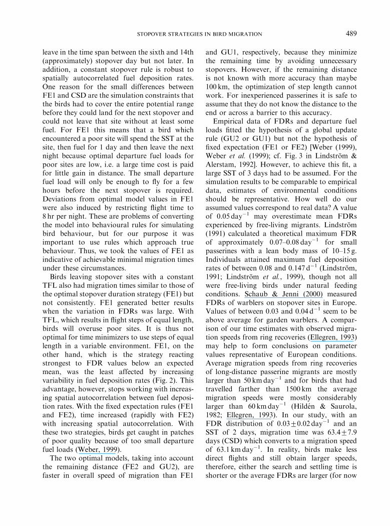
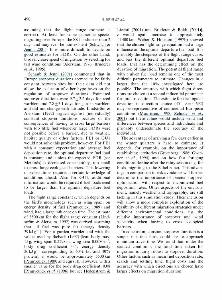
When examining only the influence of theflight range constant c and orientational accu-racy on total migration time (Figs 6 and 7),speed of migration dropped below 50 kmd�1

(mean total time larger than 80 days) for valuesof c smaller than ca. 5500 km and for an angulardeviation larger than 651 (r¼ 0.356). Up to 451the changes in time were relatively small withevery 51 increase in angular deviation, e.g. anincrease of 3.7 days in total migration time from401 to 451 (Fig. 7). With an angular deviationof 701, approximately 28% of all birds did notarrive within 100 days. At this error levelmigration duration was 90.4722.0 days.

Discussion

We compared simple stopover rules with timeminimizing models with respect to the total timetaken for migration. With a CSD, migrants

-10 -5 0 5 10

FDR 0.055FDR 0.045

d 0.033d 0.027

SST 3SST 1

CSD 9CSD 7

c 9350c 7650

r 0.756r 0.619

Direction 190°

FE1GU1

time difference (days)

-10 -5 0 5 10

FDR 0.044FDR 0.036

d 0.033d 0.027

SST 2SST 0

CSD 7CSD 5

c 7700c 6300

r 0.756r 0.619

Direction 190°

FE1GU1

time difference (days)

(a) (b)

A B

Fig. 5. Sensitivity analyses A and B. The bars are calculated as the difference in means (total migration time) betweenthe two situations (new–reference), with 95% confidence limits. The vertical axis labels indicate the values of the changedparameters. FDR: mean fuel deposition rate, d: variability in FDRs, SST: search and setting time, CSD: constant stopoverduration (days), c: flight range constant, r: directional concentration, FE1: fixed expectation rule, GU1: global update rule.(a) Sensitivity analysis A, the values for the reference situation are: FDR¼ 0.05, d ¼ 0:03; SST¼ 2 days, CSD¼ 8 days,c ¼ 8500 km, r ¼ 0:692; mean flight direction¼ 1801, stopover strategy¼CSD of 8 days. Total migration time for referencesituation A: 54.877.9 days (mean7s.d.). (b) Sensitivity analysis B, values of reference situation B: FDR¼ 0.04, d ¼ 0:03;SST¼ 1 days, CSD¼ 6 days, c ¼ 7000 km, r ¼ 0:692; mean flight direction¼ 1801, stopover strategy¼CSD of 6 days. Totalmigration time for reference situation B: 64.079.3 (mean7s.d).

0

20

40

60

80

100

120

3000 5000 7000 9000 11000 13000range constant (km)

tota

l tim

e (d

ays)

Fig. 6. Mean total migration time (7s.d.) with increas-ing flight range constant c. For each value the simulationwas repeated 20 times to elliminate the effect of maps. FDR0.0570.04 day�1, SST¼ 2, CSD¼ 10 days.

0

20

40

60

80

100

120

0 10 20 30 40 50 60 70 80angular deviation (°)

tota

l tim

e (d

ays)

Fig. 7. Mean total migration time (7s.d.) with increas-ing angular deviation in the choice of flight directions(chosen from a wrapped normal distribution withmean¼ 1801). For each value the simulation was repeated20 times to elliminated the effect of maps. FDR0.0570.04 day�1, SST¼ 2, CSD¼ 10 days.

B. ERNI ET AL.488

closely approached the optimal migration timesof the fixed expectation rule (FE1), whichdetermines the optimal departure fuel load fordifferent fuel deposition rates. With CSD andunder the examined stopover conditions, timechanged little when stopover duration changedbetween 6, 8 and 10 days and all resulting timeswere within 2.5 days of the migration durationwith FE1, except when search and settling timewas 1 day and with large variability in FDRs,

d ¼ 0:05: This flexibility is likely to be ofadvantage when other environmental factors,e.g. weather conditions, are considered in thedecision whether to leave the stopover site or not(e.g. Akesson & Hedenstrom, 2000; Danhardt& Lindstrom, 2001). It also supports thehypothesis of Weber et al. (1998) and Weber& Hedenstrom (2000) that, depending on thefrequency of good wind conditions, birds should

STOPOVER STRATEGIES IN BIRD MIGRATION 489

leave in the time span between the sixth and 14th(approximately) stopover day but not later. Inaddition, a constant stopover rule is robust tospatially autocorrelated fuel deposition rates.One reason for the small differences betweenFE1 and CSD are the simulation constraints thatthe birds had to cover the entire potential rangebefore they could land for the next stopover andcould not leave that site without at least somefuel. For FE1 this means that a bird whichencountered a poor site will spend the SST at thesite, then fuel for 1 day and then leave the nextnight because optimal departure fuel loads forpoor sites are low, i.e. a large time cost is paidfor little gain in distance. The small departurefuel load will only be enough to fly for a fewhours before the next stopover is required.Deviations from optimal model values in FE1were also induced by restricting flight time to8 hr per night. These are problems of convertingthe model into behavioural rules for simulatingbird behaviour, but for our purpose it wasimportant to use rules which approach truebehaviour. Thus, we took the values of FE1 asindicative of achievable minimal migration timesunder these circumstances.

Birds leaving stopover sites with a constantTFL also had migration times similar to those ofthe optimal stopover duration strategy (FE1) butnot consistently. FE1 generated better resultswhen the variation in FDRs was large. WithTFL, which results in flight steps of equal length,birds will overuse poor sites. It is thus notoptimal for time minimizers to use steps of equallength in a variable environment. FE1, on theother hand, which is the strategy reactingstrongest to FDR values below an expectedmean, was the least affected by increasingvariability in fuel deposition rates (Fig. 2). Thisadvantage, however, stops working with increas-ing spatial autocorrelation between fuel deposi-tion rates. With the fixed expectation rules (FE1and FE2), time increased (rapidly with FE2)with increasing spatial autocorrelation. Withthese two strategies, birds get caught in patchesof poor quality because of too small departurefuel loads (Weber, 1999).

The two optimal models, taking into accountthe remaining distance (FE2 and GU2), arefaster in overall speed of migration than FE1

and GU1, respectively, because they minimizethe remaining time by avoiding unnecessarystopovers. However, if the remaining distanceis not known with more accuracy than maybe100 km, the optimization of step length cannotwork. For inexperienced passerines it is safe toassume that they do not know the distance to theend or across a barrier to this accuracy.

Empirical data of FDRs and departure fuelloads fitted the hypothesis of a global updaterule (GU2 or GU1) but not the hypothesis offixed expectation (FE1 or FE2) [Weber (1999),Weber et al. (1999); cf. Fig. 3 in Lindstrom &Alerstam, 1992]. However, to achieve this fit, alarge SST of 3 days had to be assumed. For thesimulation results to be comparable to empiricaldata, estimates of environmental conditionsshould be representative. How well do ourassumed values correspond to real data? A valueof 0.05 day�1 may overestimate mean FDRsexperienced by free-living migrants. Lindstrom(1991) calculated a theoretical maximum FDRof approximately 0.07–0.08 day�1 for smallpasserines with a lean body mass of 10–15 g.Individuals attained maximum fuel depositionrates of between 0.08 and 0.147 d�1 (Lindstrom,1991; Lindstrom et al., 1999), though not allwere free-living birds under natural feedingconditions. Schaub & Jenni (2000) measuredFDRs of warblers on stopover sites in Europe.Values of between 0.03 and 0.04 d�1 seem to beabove average for garden warblers. A compar-ison of our time estimates with observed migra-tion speeds from ring recoveries (Ellegren, 1993)may help to form conclusions on parametervalues representative of European conditions.Average migration speeds from ring recoveriesof long-distance passerine migrants are mostlylarger than 50 kmday�1 and for birds that hadtravelled farther than 1500 km the averagemigration speeds were mostly considerablylarger than 60 kmday�1 (Hilden & Saurola,1982; Ellegren, 1993). In our study, with anFDR distribution of 0.0370.02 day�1 and anSST of 2 days, migration time was 63.477.9days (CSD) which converts to a migration speedof 63.1 kmday�1. In reality, birds make lessdirect flights and still obtain larger speeds,therefore, either the search and settling time isshorter or the average FDRs are larger (for now

B. ERNI ET AL.490

assuming that the flight range estimate iscorrect). At least for some passerine speciesmigrating over Europe, the SST is shorter than 2days and may even be non-existent (Schwilch &Jenni, 2001). It is more difficult to decide ongood estimates for FDRs. On the other hand,birds increase speed of migration by selecting fortail wind conditions (Alerstam, 1976; Brudereret al., 1995).

Schaub & Jenni (2001) commented that inEurope stopover durations seemed to be fairlyconstant between sites but their data did notallow the exclusion of other hypotheses on theregulation of stopover durations. Estimatedstopover durations were 9.772.2 days for reedwarblers and 7.873.1 days for garden warblersand did not change with latitude. Lindstrom &Alerstam (1992) argued against (individually)constant stopover durations, because of theconsequences of having to cross large barrierswith too little fuel whenever large FDRs werenot possible before a barrier, due to weather,habitat quality or other factors. FE1 or GU1would not solve this problem, however. For FE1with a constant expectation and average fueldeposition rate, the optimal departure fuel loadis constant and, unless the expected FDR (seeMethods) is decreased considerably, too smallto cross large ecological barriers. This loweringof expectations requires a certain knowledge ofconditions ahead. Also for GU1, additionalinformation would be required if fuel loads needto be larger than the optimal departure fuelloads.

The flight range constant c, which depends onthe bird’s morphology such as wing span, onenergy density of fuel (Pennycuick, 1989) andwind, had a large influence on time. The estimateof 8500 km for the flight range constant (Lind-strom & Alerstam, 1992) was derived assumingthat all fuel was pure fat (energy density39 kJ g�1). For a garden warbler and with thevalues used by Biebach (1992) (lean body mass15 g, wing span 0.2298m, wing area 0.0080m2,body drag coefficient 0.4, energy density26 kJ g�1 corresponding to 60% fat and 40%protein), c would be approximately 5500 km[Pennycuick, 1989; and eqn (3)]. However, with asmaller value for the body drag coefficient, 0.08[Pennycuick et al. (1996) but see Hedenstrom &

Liechti (2001) and Bruderer & Boldt (2001)],c would again increase to approximately11 400 km. Weber & Houston (1997b) showedthat the chosen flight range equation had a largeinfluence on the optimal departure fuel load. It isprobably the steepness of the flight range curve,and less the different optimal departure fuelloads, that has the determining effect on theduration of migration. The potential flight rangewith a given fuel load remains one of the mostdifficult parameters to estimate. Changes in c

larger than the 10% investigated here arepossible. The accuracy with which flight direc-tions are chosen is a second influential parameterfor total travel time. The estimate for the angulardeviation in direction choice (451, r ¼ 0:692)may be representative of continental Europeanconditions (Mouritsen, 1998; Zehnder et al.,2001) but these values would include wind anddifferences between species and individuals andprobably underestimate the accuracy of theindividual.

The advantage of arriving a few days earlier inthe winter quarters is hard to estimate. Itdepends, for example, on the importance ofestablishing territories (Greenberg, 1986; Gwin-ner et al., 1994) and on how fast foragingconditions decline after the rainy season (e.g. forbirds migrating to the Sahel zone). This advan-tage in comparison to risk avoidance will furtherdetermine the importance of precise stopoveroptimization with respect to encountered fueldeposition rates. Other aspects of the environ-ment, namely weather and topography, are stilllacking in this simulation study. Their inclusionwill allow a more complete exploration of thefeasibility of different migration strategies underdifferent environmental conditions, e.g. therelative importance of stopover and windselectivity when having to cross ecologicalbarriers.

In conclusion, constant stopover duration is asimple rule that birds could use to approachminimum travel time. We found that, under thestudied conditions, the total time taken formigration is fairly robust to stopover duration.Other factors such as mean fuel deposition rate,search and settling time, flight costs and theaccuracy with which directions are chosen havelarger effects on migration duration.

STOPOVER STRATEGIES IN BIRD MIGRATION 491

We thank Thomas Steuri for an introduction toVisual Basic and an initial simulation program withwhich to start. We also thank Lukas Jenni, RetoSpaar, Susanna Zehnder and two referees for theirvaluable and constructive comments on the manu-script. This study was financially supported by theSwiss National Science Foundation, Grant No. 31-43242.95.

REFERENCES

Akesson, S. & Hedenstroº m, A. (2000). Wind selectivity ofmigratory flight departures in birds. Behav. Ecol. Socio-biol. 47, 140–144.

Alerstam, T. (1976). Bird migration in relation to windand topography. Ph.D. Thesis, Lund University.

Alerstam,T. & Hedenstroº m, A. (1998). The developmentof bird migration theory. J. Avian Biol. 29, 343–369.

Alerstam, T. & Lindstroº m, A� . (1990). Optimal birdmigration: the relative importance of time, energy, andsafety. In: Bird Migration: Physiology and Ecophysiology(Gwinner, E., ed.), pp. 331-351. Berlin: Springer-Verlag.

Batschelet, E. (1981). Circular Statistics in Biology.London, New York: Academic Press.

Biebach, H. (1992). Flight-range estimates for small trans-Sahara migrants. Ibis 134, 47–54.

Bruderer, B. & Boldt, A. (2001). Flight characteristics ofbirds: I. Radar measurements of speeds. Ibis 143,178–204.

Bruderer, B., Underhill, L. G. & Liechti, F. (1995).Altitude choice of night migrants in a desert areapredicted by meteorological factors. Ibis 137, 44–55.

Charnov, E. L. (1976). Optimal foraging, the marginalvalue theorem. Theor. Popul. Biol. 9, 129–136.

Cochran, W. W., Montgomery, G. G. & Graber, R. R.(1967). Migratory flights of Hylocichla thrushes in spring:a radiotelemetry study. Living Bird 6, 213–225.

Daº nhardt, J. & Lindstroº m, A� . (2001). Optimal depar-ture decisions of songbirds from an experimental stop-over site and the significance of weather. Anim. Behav. 62,235–243, doi: 10.1006/anbe.2001.1749.

Ellegren, H. (1993). Speed of migration and migratoryflight lengths of passerine birds ringed during autumnmigration in Sweden. Ornis Scand. 24, 220–228.

Erni, B., Liechti, F. & Bruderer, B. (2002). Wind andrain govern the intensity of nocturnal bird migration incentral Europe F a log-linear regression analysis. Ardea90, 155–166.

Greenberg, R. (1986). Competition in migrant birds in thenonbreeding season. In: Current Ornithology (Johnston,R. F., ed.), pp. 281-307. New York, London: PlenumPress.

Gwinner, E., Roº dl, T. & Schwabl, H. (1994). Pairterritoriality of wintering stonechats: behaviour, funtionand hormones. Behav. Ecol. Sociobiol. 34, 321–327.

Hedenstroº m, A. & Alerstam, T. (1997). Optimum fuelloads in migratory birds: distinguishing between time andenergy minimization. J. theor. Biol. 189, 227–234.

Hedenstroº m, A. & Liechti, F. (2001). Field estimate ofbody drag coeffiecient on the basis of dives in passerinebirds. J. Exp. Biol. 204, 1167–1175.

Hedenstroº m, A. & Weber, T. P. (1999). Gone with thewind? A comment on Butler et al. (1997). Auk 116,

560–562.HildeŁ n, O. & Saurola, P. (1982). Speed of autumn

migration of birds ringed in Finland. Ornis Fennica 59,

140–142.Houston, A. I. (1998). Models of optimal avian

migration: state, time and predation. J. Avian Biol. 29,

395–404.Klaassen, M. & Biebach, H. (1994). Energetics of

fattening and starvation in the long-distance migratorygarden warbler, Sylvia borin, during the migratory phase.J. Comp. Physiol. B 164, 362–371.

Klaassen, M. & Lindstroº m, A. (1996). Departure fuelloads in time-minimising migrating birds can be ex-plained by the energy costs of being heavy. J. theor. Biol.183, 29–34.

Liechti, F. (1992). Flugverhalten nachtlich ziehenderVogel in Abhangigkeit von Wind und Topographie.Ph.D. Dissertation, Basel University, Basel.

Liechti, F. & Bruderer, B. (1995). Direction, speed andcomposition of nocturnal bird migration in the south ofIsrael. Isr. J. Zool. 41, 501–515.

Lindstroº m, A. (1991). Maximum fat deposition rates inmigrating birds. Ornis Scand. 22, 12–19.

Lindstroº m, A. & Alerstam, T. (1992). Optimal fat loadsin migrating birds: a test of the time-minimizationhypothesis. Am. Nat. 140, 477–491.

Lindstroº m, A. Klaassen, M. & Kvist, A. (1999).Variation in energy intake and basal metabolic rateof a bird migrating in a wind tunnel. Funct. Ecol. 13,

352–359.Mouritsen, H. (1998). Modelling migration: the clock-

and-compass model can explain the distribution ofringing recoveries. Anim. Behav. 56, 899–907.

Pennycuick, C. J. (1989). Bird Flight Performance: APractical Calculation Manual. Oxford: Oxford UniversityPress.

Pennycuick, C. J., Klaassen, M., Kvist, A. & Lind-stroº m, A. (1996). Wingbeat frequency and the bodydrag anomaly: wind-tunnel observations on a ThrushNightingale (Luscinia luscinia) and Teal (Anas crecca).J. Exp. Biol. 199, 2757–2765.

Piersma, T. & Jukema, J. (1990). Budgeting the flight of along-distance migrant: changes in nutrient reserve levelsof Bar-tailed Godwits at successive spring staging sites.Ardea 78, 315–337.

Rice, J. A. (1988). Mathematical Statistics and DataAnalysis. Belmont, CA: Wadsworth.

Schaub, M. & Jenni, L. (2000). Fuel deposition of threepasserine bird species along the migration route. Oeco-logia 122, 306–317.

Schaub, M. & Jenni, L. (2001). Stopover durations ofthree warbler species along their autumn migration route.Oecologia 128, 217–227.

Schwilch, R. & Jenni, L. (2001). Low initial refuellingrate at stopover sites: a methodological effect? Auk 118,698–708.

Weber, T. P. (1999). Blissful ignorance? Departure rulesfor migrants in a spatially heterogeneous environment.J. theor. Biol. 199, 415–524, doi: jtbi.1999.0968.

Weber, T. P. & Hedenstroº m, A. (2000). Optimal stopoverdecisions under wind influence: the effects of correlatedwinds. J. theor. Biol. 205, 95–104, doi: 10.1006/jtbi.2000.2047.

B. ERNI ET AL.492

Weber, T. P. & Houston, A. I. (1997a). A general modelfor time-minimising avian migration. J. theor. Biol. 185,447–458.

Weber, T. P. & Houston, A. I. (1997b). Flight costs, flightrange and the stopover ecology of migrating birds.J. Anim. Ecol. 66, 297–306.

Weber, T. P., Alerstam, T. & Hedenstroº m, A. (1998).Stopover decisions under wind influence. J. Avian Biol.29, 552–560.

Weber, T. P., Fransson, T. & Houston, A. I. (1999).Should I stay or should I go? Testing optimality modelsof stopover decisions in migrating birds. Behav. Ecol.Sociobiol. 46, 280–286.

Zehnder, S., Akesson, S., Liechti, F. & Bruderer, B.(2001). Nocturnal autumn bird migration at Falsterbo,south Sweden. J. Avian Biol. 32, 239–248.

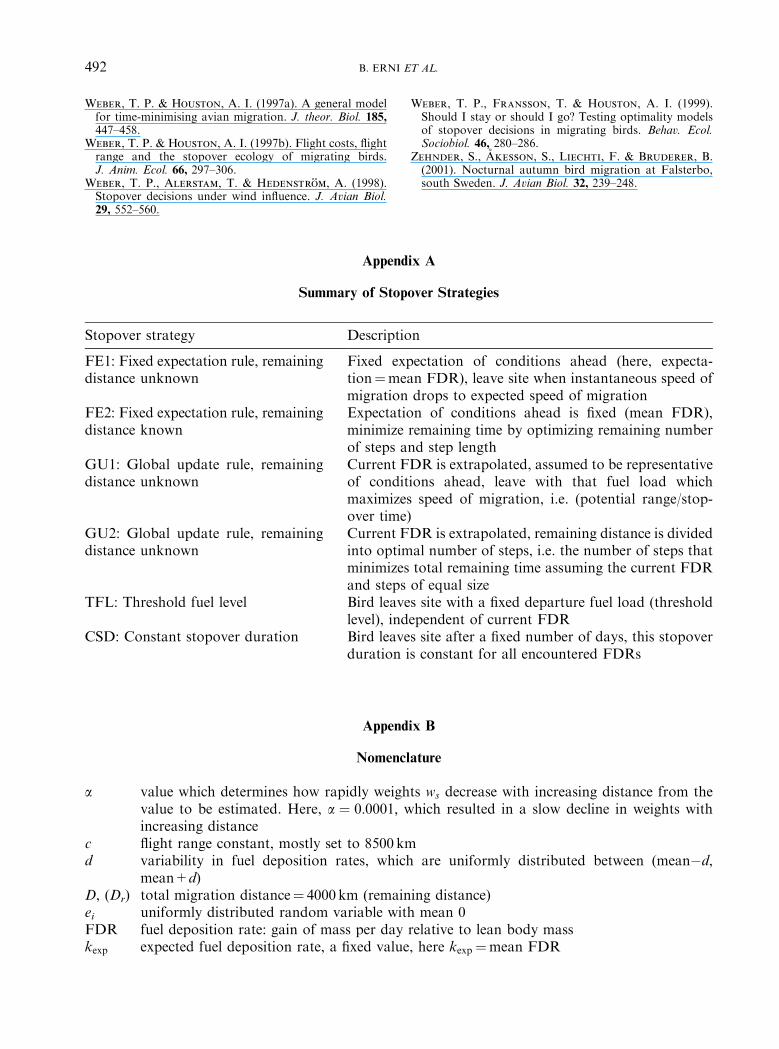
Appendix A

Summary of Stopover Strategies

Stopover strategy Description

FE1: Fixed expectation rule, remainingdistance unknown

Fixed expectation of conditions ahead (here, expecta-tion¼mean FDR), leave site when instantaneous speed ofmigration drops to expected speed of migration

FE2: Fixed expectation rule, remainingdistance known

Expectation of conditions ahead is fixed (mean FDR),minimize remaining time by optimizing remaining numberof steps and step length

GU1: Global update rule, remainingdistance unknown

Current FDR is extrapolated, assumed to be representativeof conditions ahead, leave with that fuel load whichmaximizes speed of migration, i.e. (potential range/stop-over time)

GU2: Global update rule, remainingdistance unknown

Current FDR is extrapolated, remaining distance is dividedinto optimal number of steps, i.e. the number of steps thatminimizes total remaining time assuming the current FDRand steps of equal size

TFL: Threshold fuel level Bird leaves site with a fixed departure fuel load (thresholdlevel), independent of current FDR

CSD: Constant stopover duration Bird leaves site after a fixed number of days, this stopoverduration is constant for all encountered FDRs

Appendix B

Nomenclature

a value which determines how rapidly weights ws decrease with increasing distance from thevalue to be estimated. Here, a ¼ 0:0001; which resulted in a slow decline in weights withincreasing distance

c flight range constant, mostly set to 8500 kmd variability in fuel deposition rates, which are uniformly distributed between (mean�d,

mean+d)D, (Dr) total migration distance¼ 4000 km (remaining distance)ei uniformly distributed random variable with mean 0FDR fuel deposition rate: gain of mass per day relative to lean body masskexp expected fuel deposition rate, a fixed value, here kexp ¼mean FDR

STOPOVER STRATEGIES IN BIRD MIGRATION 493

ki; ð %kÞ fuel deposition rate in cell i (overall mean fuel deposition rate)n; (nn) number (optimal number) of remaining flight steps till ends distance (in number of cells)SST search and settling time (days)t; (tn) stopover duration (optimal stopover duration)te search and settling timeWs weight for the contribution of a distant cell to the value in cell i (for autocorrelated FDRs).

ws decreases with increasing distance from cell i [see eqn (2)]x fuel load (relative to lean body mass)Y ðxÞ flight range with fuel load x (km)