Stochastic Modeling of WiFi's EDCA and Double Frequency ...

HAL Id: pastel-00561406https://pastel.archives-ouvertes.fr/pastel-00561406

Submitted on 1 Feb 2011

HAL is a multi-disciplinary open accessarchive for the deposit and dissemination of sci-entific research documents, whether they are pub-lished or not. The documents may come fromteaching and research institutions in France orabroad, or from public or private research centers.

L’archive ouverte pluridisciplinaire HAL, estdestinée au dépôt et à la diffusion de documentsscientifiques de niveau recherche, publiés ou non,émanant des établissements d’enseignement et derecherche français ou étrangers, des laboratoirespublics ou privés.

Stochastic Modeling of WiFi’s EDCA and DoubleFrequency Reuse for Femtocell

Yoram Haddad

To cite this version:Yoram Haddad. Stochastic Modeling of WiFi’s EDCA and Double Frequency Reuse for Femtocell.Networking and Internet Architecture [cs.NI]. Télécom ParisTech, 2010. English. �pastel-00561406�

Thèse

présentée pour obtenir le grade de Docteur de Télécom ParisTech

Spécialité : Informatique et Réseaux

Yoram HADDAD

Modélisation Stochastique du Mécanisme EDCA du WiFi et Double Réutilisation de Fréquences pour les

Femtocells

Soutenue le 13 Septembre 2010 devant le jury composé de

Pr. Samir Tohme Président

Pr. André-Luc Beylot Rapporteurs

Pr. Jay Weitzen

Pr .Simon Bloch Examinateur

M. Jacques Bensimon

Pr. Noémie Simoni Directeurs de thèse

Dr .Gwendal Le Grand

PhD Thesis

Dissertation submitted in partial fulfillment of the requirement for the degree of

Doctor of Philosophy

of Graduate School TELECOM ParisTech

In: Computer Science and Networks

by Yoram HADDAD

Modeling of WiFi's EDCA and Double frequency reuse for Femtocell

Presented the 13th of September 2010 before the jury composed of

Prof. Samir Tohme President

Prof. André-Luc Beylot Reviewer

Prof. Jay Weitzen Reviewer

Prof. Simon Bloch Examiner

M. Jacques Bensimon Examiner

Prof. Noémie Simoni Advisor

Dr . Gwendal Le Grand Advisor

Contents

List of Figures 6

List of Tables 8

Glossary 9

Acknowledgements 14

Abstract 16

Resume-French Synthesis 17

1 Introduction 511.1 ”Ubiquitous Wireless” . . . . . . . . . . . . . . . . . . . . . . 511.2 Challenges . . . . . . . . . . . . . . . . . . . . . . . . . . . . . 52

1.2.1 Capacity Evaluation of a Wifi Cell . . . . . . . . . . . 531.2.2 Qos Parameters for WiFi . . . . . . . . . . . . . . . . 53

1.3 Thesis Goals and Contributions . . . . . . . . . . . . . . . . . 541.3.1 Stochastic Model for Wifi Access . . . . . . . . . . . . 541.3.2 Femtocell . . . . . . . . . . . . . . . . . . . . . . . . . 55

1.4 Thesis Outline . . . . . . . . . . . . . . . . . . . . . . . . . . 56

I Background and state of the ART 57

2 Access Mechanisms to IEEE 802.11 WiFi Networks andTheir Analytical Model 592.1 MAC of the IEEE 802.11 and 802.11e description . . . . . . 59

2.1.1 introduction . . . . . . . . . . . . . . . . . . . . . . . . 592.1.2 Distributed Coordination Function . . . . . . . . . . . 61

3

2.1.3 Enhanced Distributed Coordinated Access function . . 632.2 State of The ART . . . . . . . . . . . . . . . . . . . . . . . . 65

2.2.1 Seminal Models . . . . . . . . . . . . . . . . . . . . . . 662.2.2 DCF models . . . . . . . . . . . . . . . . . . . . . . . 672.2.3 EDCA models . . . . . . . . . . . . . . . . . . . . . . 682.2.4 Summary Table . . . . . . . . . . . . . . . . . . . . . . 68

3 Frequency Allocation to Femtocell 703.1 Introduction . . . . . . . . . . . . . . . . . . . . . . . . . . . . 703.2 Description . . . . . . . . . . . . . . . . . . . . . . . . . . . . 71

3.2.1 Access Control . . . . . . . . . . . . . . . . . . . . . . 723.3 Challenges . . . . . . . . . . . . . . . . . . . . . . . . . . . . . 73

3.3.1 Femtocell to Macrocell Downlink Interference . . . . . 733.3.2 Macrocell to Femtocell Uplink Interference . . . . . . 733.3.3 Femtocell to Femtocell Uplink Interference . . . . . . 743.3.4 Femtocell to Femtocell Downlink Interference . . . . . 74

3.4 Existing Allocation Scheme . . . . . . . . . . . . . . . . . . . 743.4.1 Introduction . . . . . . . . . . . . . . . . . . . . . . . 753.4.2 Experimental Results in the Literature . . . . . . . . . 763.4.3 Cross-Tier Allocation Scheme . . . . . . . . . . . . . . 763.4.4 Co-tier allocation scheme . . . . . . . . . . . . . . . . 79

II Our Proposition 83

4 Stochastic Model of EDCA 844.1 System Model . . . . . . . . . . . . . . . . . . . . . . . . . . . 84

4.1.1 Four Dimensional Markov Chain . . . . . . . . . . . . 844.1.2 Markov Chain . . . . . . . . . . . . . . . . . . . . . . 874.1.3 Characteristic of Our Model: the Unsaturated Mode . 884.1.4 Transition probabilities . . . . . . . . . . . . . . . . . 884.1.5 Probability in steady state and equation systems . . . 93

4.2 Throughput derivation . . . . . . . . . . . . . . . . . . . . . . 1024.3 Delay derivation . . . . . . . . . . . . . . . . . . . . . . . . . 103

5 Frequency allocation to femtocell a double frequency reuseassignment scheme 1065.1 Double Frequency Reuse: A novel Channel Allocation Scheme

for Femtocells . . . . . . . . . . . . . . . . . . . . . . . . . . . 1065.2 Femtocell’s Channel Selection . . . . . . . . . . . . . . . . . . 109

4

5.3 Other Fundamentals Parameters . . . . . . . . . . . . . . . . 1095.3.1 Radio Resource Granularity . . . . . . . . . . . . . . . 1105.3.2 Femtocell Transmission Power . . . . . . . . . . . . . 1125.3.3 Adjacent Channel Interference . . . . . . . . . . . . . 113

III Results 114

6 Analytical Results of the Stochastic Model of EDCA 1156.1 Equations System . . . . . . . . . . . . . . . . . . . . . . . . . 1156.2 Unsaturated mode and error prone channel effects on the

throughput . . . . . . . . . . . . . . . . . . . . . . . . . . . . 1186.3 AIFS and CWmin differentiation mechanism . . . . . . . . . 122

6.3.1 AIFS mechanism . . . . . . . . . . . . . . . . . . . . . 1226.3.2 CWmin mechanism . . . . . . . . . . . . . . . . . . . 122

6.4 Some delay results . . . . . . . . . . . . . . . . . . . . . . . . 124

7 Simulation and Results for Femtocell Channels Reuse 1297.1 Performance derivation . . . . . . . . . . . . . . . . . . . . . . 1297.2 Simulation Parameters . . . . . . . . . . . . . . . . . . . . . . 130

7.2.1 Propagation Models . . . . . . . . . . . . . . . . . . . 1317.3 Macrocell-Femtocell Simulator . . . . . . . . . . . . . . . . . 1327.4 Results . . . . . . . . . . . . . . . . . . . . . . . . . . . . . . . 139

7.4.1 Introduction . . . . . . . . . . . . . . . . . . . . . . . 1397.4.2 Femtocell RSS Performance . . . . . . . . . . . . . . . 1407.4.3 Femtocell SINR Performance . . . . . . . . . . . . . . 1447.4.4 Effect of the Transmission Power . . . . . . . . . . . . 146

8 Conclusion 153

9 Appendix :Fixed Point Theorem Method 157

Bibliography 161

Publications 169

5

List of Figures

2.1 DCF interframe space . . . . . . . . . . . . . . . . . . . . . . 622.2 DCF access method . . . . . . . . . . . . . . . . . . . . . . . 622.3 RTS-CTS protection and NAV . . . . . . . . . . . . . . . . . 622.4 MAC architecture . . . . . . . . . . . . . . . . . . . . . . . . 642.5 Mapping to one of the AC . . . . . . . . . . . . . . . . . . . . 652.6 AIFS prioritization mechanism of EDCA . . . . . . . . . . . 66

3.1 Femtocell-to-Femtocell Uplink Attack . . . . . . . . . . . . . 74

4.1 A Frozen Period . . . . . . . . . . . . . . . . . . . . . . . . . 864.2 Collisions and Errors . . . . . . . . . . . . . . . . . . . . . . . 874.3 The full Markov chain . . . . . . . . . . . . . . . . . . . . . . 1004.4 Simplified Markov Chain . . . . . . . . . . . . . . . . . . . . . 101

5.1 Frequency reuse scheme . . . . . . . . . . . . . . . . . . . . . 108

6.1 Throughput under different traffic loads . . . . . . . . . . . . 1196.2 Throughput under different error-prone environments vs. packet

size . . . . . . . . . . . . . . . . . . . . . . . . . . . . . . . . . 1206.3 Throughput vs. Number of active stations in unsaturated

mode . . . . . . . . . . . . . . . . . . . . . . . . . . . . . . . 1216.4 Impact of AIFS differentiation on the throughput in saturated

mode . . . . . . . . . . . . . . . . . . . . . . . . . . . . . . . . 1236.5 AIFS differentiation under different traffic loads . . . . . . . . 1246.6 Impact of CWmin differentiation on the throughput in satu-

rated mode . . . . . . . . . . . . . . . . . . . . . . . . . . . . 1256.7 CWmin differentiation under different traffic loads . . . . . . 1266.8 Delay differentiation under different traffic loads . . . . . . . 1286.9 Delay experienced with different number of stations . . . . . 128

7.1 first interface to the simulator: entering initial parameters . . 133

6

7.2 Distribution of MUE, and FAP . . . . . . . . . . . . . . . . . 1347.3 Selection of the scheme . . . . . . . . . . . . . . . . . . . . . . 1357.4 Mixed Scheme display . . . . . . . . . . . . . . . . . . . . . . 1367.5 Patial scheme display . . . . . . . . . . . . . . . . . . . . . . . 1377.6 Display of Uplink results . . . . . . . . . . . . . . . . . . . . . 1387.7 Display of Downlink results . . . . . . . . . . . . . . . . . . . 1387.8 Numerical Results for RSS and SINR . . . . . . . . . . . . . . 1397.9 RSS in Downlink with uniform distribution . . . . . . . . . . 1417.10 RSS in Uplink with uniform distribution . . . . . . . . . . . . 1417.11 RSS in Downlink with concentration at the edge . . . . . . . 1427.12 RSS in Uplink with concentration at the edge . . . . . . . . . 1427.13 RSS in Downlink with concentration in the center . . . . . . 1437.14 RSS in Uplink with concentration in the center . . . . . . . . 1437.15 Downlink SINR with uniform distribution . . . . . . . . . . . 1447.16 Uplink SINR with uniform distribution . . . . . . . . . . . . . 1457.17 Downlink SINR CDF with uniform distribution . . . . . . . . 1457.18 Uplink SINR CDF with uniform distribution . . . . . . . . . 1467.19 Downlink SINR with edge deployment . . . . . . . . . . . . . 1477.20 Uplink SINR with edge deployment . . . . . . . . . . . . . . . 1477.21 Effect of the MAP Tx power on the RSS femtocell Downlink

transmission . . . . . . . . . . . . . . . . . . . . . . . . . . . . 1487.22 Effect of the MAP Tx power on the SINR femtocell Downlink

transmission . . . . . . . . . . . . . . . . . . . . . . . . . . . . 1487.23 Effect of the FAP Tx power on the RSS femtocell Downlink

transmission . . . . . . . . . . . . . . . . . . . . . . . . . . . . 1497.24 Effect of the FAP Tx power on the SINR femtocell Downlink

transmission . . . . . . . . . . . . . . . . . . . . . . . . . . . . 1507.25 Effect of the MUE Tx power on the RSS femtocell Uplink

transmission . . . . . . . . . . . . . . . . . . . . . . . . . . . . 1507.26 Effect of the MUE Tx power on the SINR femtocell Uplink

transmission . . . . . . . . . . . . . . . . . . . . . . . . . . . . 1517.27 Effect of the FUE Tx power on the RSS femtocell Uplink

transmission . . . . . . . . . . . . . . . . . . . . . . . . . . . . 1527.28 Effect of the FUE Tx power on the SINR femtocell Uplink

transmission . . . . . . . . . . . . . . . . . . . . . . . . . . . . 152

7

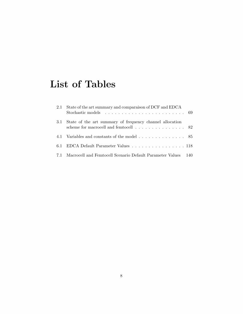
List of Tables

2.1 State of the art summary and comparaison of DCF and EDCAStochastic models . . . . . . . . . . . . . . . . . . . . . . . . 69

3.1 State of the art summary of frequency channel allocationscheme for macrocell and femtocell . . . . . . . . . . . . . . . 82

4.1 Variables and constants of the model . . . . . . . . . . . . . . 85

6.1 EDCA Default Parameter Values . . . . . . . . . . . . . . . . 118

7.1 Macrocell and Femtocell Scenario Default Parameter Values 140

8

9

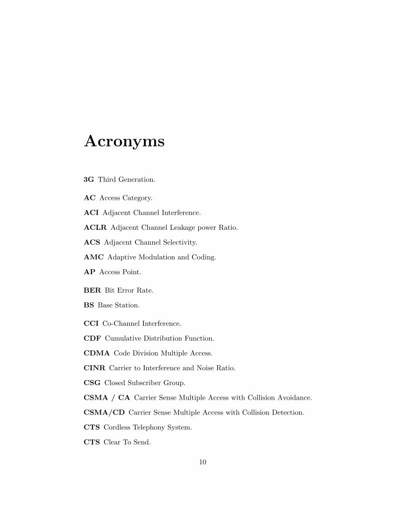
Acronyms

3G Third Generation.

AC Access Category.

ACI Adjacent Channel Interference.

ACLR Adjacent Channel Leakage power Ratio.

ACS Adjacent Channel Selectivity.

AMC Adaptive Modulation and Coding.

AP Access Point.

BER Bit Error Rate.

BS Base Station.

CCI Co-Channel Interference.

CDF Cumulative Distribution Function.

CDMA Code Division Multiple Access.

CINR Carrier to Interference and Noise Ratio.

CSG Closed Subscriber Group.

CSMA / CA Carrier Sense Multiple Access with Collision Avoidance.

CSMA/CD Carrier Sense Multiple Access with Collision Detection.

CTS Cordless Telephony System.

CTS Clear To Send.

10

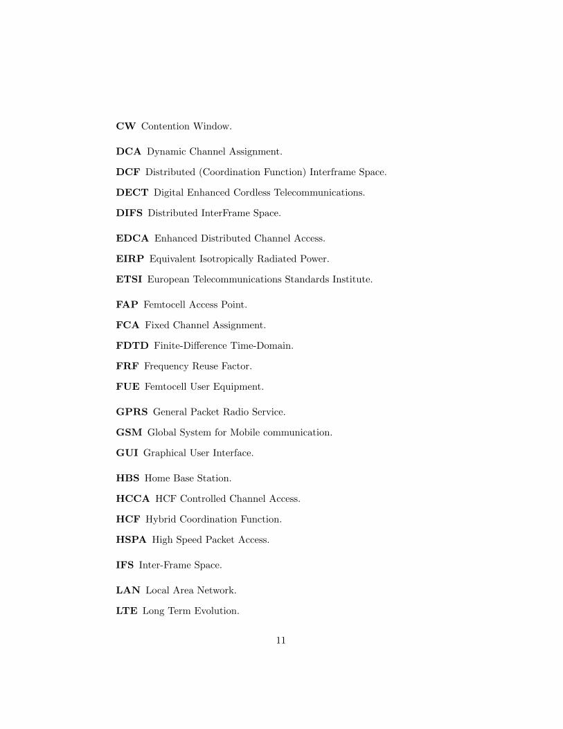
CW Contention Window.

DCA Dynamic Channel Assignment.

DCF Distributed (Coordination Function) Interframe Space.

DECT Digital Enhanced Cordless Telecommunications.

DIFS Distributed InterFrame Space.

EDCA Enhanced Distributed Channel Access.

EIRP Equivalent Isotropically Radiated Power.

ETSI European Telecommunications Standards Institute.

FAP Femtocell Access Point.

FCA Fixed Channel Assignment.

FDTD Finite-Difference Time-Domain.

FRF Frequency Reuse Factor.

FUE Femtocell User Equipment.

GPRS General Packet Radio Service.

GSM Global System for Mobile communication.

GUI Graphical User Interface.

HBS Home Base Station.

HCCA HCF Controlled Channel Access.

HCF Hybrid Coordination Function.

HSPA High Speed Packet Access.

IFS Inter-Frame Space.

LAN Local Area Network.

LTE Long Term Evolution.

11

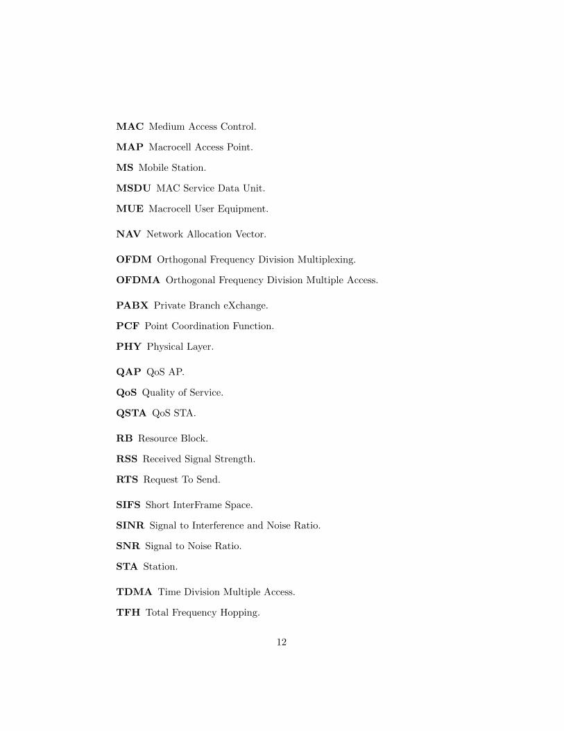
MAC Medium Access Control.

MAP Macrocell Access Point.

MS Mobile Station.

MSDU MAC Service Data Unit.

MUE Macrocell User Equipment.

NAV Network Allocation Vector.

OFDM Orthogonal Frequency Division Multiplexing.

OFDMA Orthogonal Frequency Division Multiple Access.

PABX Private Branch eXchange.

PCF Point Coordination Function.

PHY Physical Layer.

QAP QoS AP.

QoS Quality of Service.

QSTA QoS STA.

RB Resource Block.

RSS Received Signal Strength.

RTS Request To Send.

SIFS Short InterFrame Space.

SINR Signal to Interference and Noise Ratio.

SNR Signal to Noise Ratio.

STA Station.

TDMA Time Division Multiple Access.

TFH Total Frequency Hopping.

12

UE User Equipment.

UMTS Universal Mobile Telecommunication System.

UWB Ultra Wide Band.

VoIP Voice Over IP.

WiFi Wireless Fidelity.

WiMAX Wireless Interoperability for Microwave Access.

WLAN Wireless LAN.

13

Acknowledgements

In my humble opinion, the basis for healthy human relationships is, the abil-ity to recognize and appreciate all the good things we receive from others.So it is with a special pleasure, that with the achievement of this thesis, Iuse the opportunity to thank the people without whom this project wouldprobably never have been completed.

First and foremost, I would like to thank the almighty, creator of theworld, our G-od the holy blessed be he, for giving me the opportunity tosanctify his name in this world, to live in my father’s land and perpetuateour tradition. My thanks also go to all of his emissaries:

To Prof. Daniel Kofman for allowing me to start this project, and forhaving led me towards interesting topics with great potential and to Prof.HG Mendelbaum for all the help he provided me from a logistical point ofview and for having initiated this project.

To all the team of the Jerusalem College of Technology for their warmwelcome, their constant encouragements, technical and financial support,especially: the President Prof. Noah Dana-Picard, the Rector Prof. Men-achem Steiner, the Head of Computer Sc. Dept Dr. Motti Reif, and also tomy colleagues Drs: A. Heuman, H. Dayan, I. Kidron, Y. Peretz, Y. Hacohen-Kerner, and S. Weinman. Finally to our best secretary, who is always willingto help in every circumstances: Mrs Chana Touitou.

My gratitude goes to Dr. Gwendal Le Grand, who supervised a largepart of the thesis and from who I truly learned the job of a researcher.Thank you for your support, your confidence in my abilities (even thoughI sometimes lacked its). A big thank you to my ”professional parents” whofollowed me during this long ”trip” and encouraged me : to Prof. NoemieSimoni for supervising the thesis and to Jacques Bensimon, for all his efforts

14

to allow me to finish this thesis.

My sincere thanks to Dr. Dana Porrat for welcoming and mentoring meduring my visit at the Hebrew University of Jerusalem. Thank you for thefruitful discussions that have undoubtly permitted the completion of thisproject. Thank you to my dear childhood friend David Cabessa for makingthe best review of the English grammar work ever realized ...

I wish to thank the members of the jury chaired by Prof. Samir Tohme.To Profs Andre-Luc Beylot and Jay Weitzen for their thorough and com-prehensive reports of this manuscript. To Prof Simon Bloch who was one ofthe examiners.

My warm thanks go to my parents in-law, Pierre and Annie Rubini, whohelped us during all these years. To my uncles Hamiel, Yoski and Yoav forhaving always considered me as their own son and encouraged me to excel.

I would like to express my deep gratitude to my Rabbis who supportedand encouraged me to finish the thesis, RAVs: Zvi I. Tau, Hannane Edel-stein, David Giami, Amiel and Mordechai Sternberg, Joshua Zukerman.They are all for me a source of inspiration and moral support.

I want to express my deep gratitude to my parents who always ensuredmy well-being. You have given me confidence since my youth. This workis dedicated to you, and was worth it, even for the sole sake of seeing youreyes shine at the end of my PhD defense ... Thanks to my sister Avigaeland her husband Shay for their support at any time, day and ...night

My final thanks go to my dearest wife, Sarah, at my side at all times.Thank you for your support, your encouragements, especially in difficulttimes. Thank you for the wonderful education you have given our children,often without me, during these long years. For all these long weeks, monthsand years when I was ”just passing” at home. I apologize to my wonderfulchildren for not being able to follow them during all these years, to: Shlomo(alias ”shlomikoto ”), Yehoudith (”kimo”), Hanna (” noun ”) and Tsipora (”chips”).

Thank you my G-od for your infinite goodness renewed every day

15

Abstract

The race toward higher throughputs for cellular network users isgetting more difficult every day. On the one hand cellular network op-erators wish to increase benefits by offering new services to more users,while on the other hand spare radio resources are shrinking away. Thespreading of WiFi-3G dual mode devices is making this fight evenharder for the cellular operator. When arriving at home, users withdual mode devices automatically switch to their local wireless broad-band connection, and make free calls through Voice over IP software.The new ”Femtocell” technology is expected to be the rescuer of cel-lular network operators. This ”home” cellular base station provideshigh indoor coverage and throughput to indoor users over the regularhome broadband access connection to the internet. In this thesis, weevaluate the capacity that can be offered by the WiFi and Femtocelltechnologies separately. In the first part we propose a realistic andcomprehensive model to analyze the performance of the IEEE 802.11eEnhanced Distributed Channel Access (EDCA) contention based ac-cess mechanism, which provides class-based Quality of Service (QoS)to IEEE 802.11 Wireless LANs (WLANs). Our analytical approach isbased on Markov chains. Our innovation is that our model allows fornon-ideal channels and unsaturated networks. The improved modelallows computing and representing the performance more precisely forvarious traffic loads and various Bit Error Rates (BERs). Then weassess the performance of the femtocell approach. For this purpose,we first needed to deal with the radio planning issue. This latter issueis not obvious for a plug-and-play Femtocell device whose deploymentwill inherently be unpredictable. We propose a double frequency reusescheme, which allows a femtocell to reuse the frequency already inuse by adjacent sectors of the overlaying macrocell. We present threesolutions: full, partial or mixed frequency reuse. Then we evaluatethe performance that Femtocells can achieve when coexisting with anoverlaying macrocell in terms of RSS and SINR expected at the femto-cell level. We show that Femtocells can definitely provide a meaning-ful improvement in the data rates experienced by the femtocell user’sequipment.

16

Remerciements

La base de relations humaines saines est a mon humble avis la capacite de re-connaitre et apprecier le bien que la societe et les individus nous prodiguent.Ainsi c’est avec une satisfaction particuliere que je peux, a l’aboutissementde cette these remercier les personnes sans qui ce projet n’aurait surementpas abouti.

En tout premier lieu, je remercie le tout puissant, createur du monde,notre d.ieu le saint beni soit-il, de m’avoir donne la possibilite de sanctifierson nom dans ce monde, de vivre dans ma terre ancestrale et de perpetuernotre tradition. Mes remerciements vont egalement a l’ensemble de ses en-voyes :

Au prof Daniel Kofman pour m’avoir permis de demarrer ce projet, etpour m’avoir dirige vers des sujets interessants et a fort potentiel. Au profH.G. Mendelbaum, pour m’avoir aide d’un point de vue logistique et qui futl’initiateur du projet. A toutes les equipes du Jerusalem College of Tech-nology, pour leur accueil chaleureux, leur encouragements permanents, leursoutien technique, logistique et financier, en particulier au president profNoah Dana-Picard, au recteur Prof Menachem Steiner, au chef du dept DrMotti Reif, ansi qu’a mes collegues Dr A. Heuman, H. Dayan, Y. Peretz, Y.Hacohen-Kerner, et S. Weinman. Enfin a la personne devouee qui nous aideen toute discretion : Chana Touitou.

Mes remerciements vont au Dr. Gwendal le Grand, qui a encadre unegrande partie de la these et de qui j’ai appris veritablement le metier dechercheur. Merci pour ton soutien, ta confiance en mes capacites (meme simoi-meme je n’etais pas confiant), ta rapidite de reponse aux e-mails (ouica aussi ca aide beaucoup . . . .).

Un grand merci a mes ”parents professionnels” qui m’ont suivi et encour-

17

age durant ce long parcours. Au prof Noemi Simoni pour avoir encadre lathese et avoir permis l’aboutissement de ce periple marathon. A JacquesBenSimon, pour m’avoir encourage a conclure un travail entame.

Mes sinceres remerciement au Dr Dana Porrat pour m’avoir accueilli etencadre durant ma visite a l’universite hebraıque d’un point de vue tech-nique et financier. Merci pour ces discussions fructueuses qui ont sans doutepermis l’achevement de ce projet. Merci a mon cher ami d’enfance DavidCabessa pour avoir effectue le meilleur travail de correction jamais realise. . . .

Je souhaite remercier les membres du jury preside par le prof SamirTohme. Notamment les profs Andre-Luc Beylot et Jay Weitzen pour leurrapport complet et minutieux de ce manuscrit. Le prof S. Bloch pour avoiraccepte d’etre examinateur.

Mes chaleureux remerciements vont a mes beaux parents Pierre et AnnieRubini qui nous ont aide durant toutes ces annees. A mes oncles Hamiel,Yoski et Yoav pour m’avoir toujours suivi comme leur propre fils et encour-age a me depasser.

Je tiens a exprimer ma profonde gratitude envers mes parents qui onttoujours veille a mon bien-etre. Vous m’avez donne confiance depuis monplus jeune age. Ce travail vous est consacre, ne serait-ce que pour voir vosyeux briller au moment de ma soutenance, . . . Merci a ma soeur Avigael etmon beau frere Shay pour leur soutien a tout heure du jour et . . . de la nuit.

Je desire exprimer ma profonde gratitude envers mes Rabbins qui m’ontsoutenu et encourage a terminer la these, Rav: Zvi I. Tau, Hannane Edel-stein, David Giami, Amiel et Mordehai Sternberg, Yehochoua Zukerman. Ilssont tous pour moi une source d’inspiration et de support moral intarissable.

Enfin mes derniers remerciements, les plus chers, vont a ma femme Sarah,a mes cotes en toutes circonstances. Merci pour ton soutien, tes encourage-ments dans les moments difficiles. Merci pour l’education merveilleuse quetu as donne a nos enfants, souvent sans moi durant ces longues annees. Pourtoutes ces longues semaines, mois et annees ou je n’etais ”que de passage” ala maison. Je demande pardon a mes merveilleux enfants de ne pas avoir pules suivre durant toutes ces annees, a : Shlomo (”shlomikoto”), Yehoudith(”kimo”), Hanna (”noun”) et Tsipora (”chips”).

Merci mon d.ieu pour ta bonte infinie renouvellee tout les jours.

18

Resume de la these enFrancais - Short Version ofthe Thesis in French

La course vers des debits plus eleves pour les utilisateurs de reseaux cellu-laires devient plus difficile chaque jour. Les operateurs de reseaux cellulairessouhaitent accroitre leurs benefices en offrant de nouveaux services a unnombre croissant d’utilisateurs, mais la ressource radio disponible diminueen permanence. Le developpement de telephone cellulaire surnomme enanglais ”dual-mode” (bi-mode) qui abrite au sein d’un meme appareil lestechnologies cellulaires et le Wifi rend cette lutte encore plus ardue. Enarrivant a la maison, un utilisateur disposant d’un appareil ”bi-mode” bas-culera forcement vers sa connexion locale sans fil a haut debit et pourraainsi jouir de services d’appels gratuits via des logiciels de Voix sur IP. Lanouvelle technologie surnommee ”Femtocell” est consideree comme le poten-tiel sauveur des operateurs menaces par la concurrence du Wifi. Ce pointd’acces residentiel au reseau cellulaire offre une meilleure couverture et unplus haut debit aux utilisateurs situes en interieur. Dans cette these, nousevaluons separement, la capacite utile offerte par un point d’acces Wifi etpar un point d’acces ”Femtocell”. Dans la premiere partie nous proposons unmodele realiste du mecanisme d’acces a la ressource du Wifi. Ce mecanismeconnu sous l’acronyme EDCA prevoit une differentiation des services requispar l’utilisateur. Notre modele est base sur les chaınes de Markov. Notre evi-tons les principales approximations faites dans les modeles anterieurs. Nousprenons en compte, un regime non sature en prenant en compte un canalnon ideal. Ainsi nous pouvons obtenir les performances attendues avec plusde precision pour differentes charges de trafic et divers taux d’erreur binaire(BER). Dans un second temps nous evaluons les performances des Femtocell.Pour ce, nous avons tout d’abord propose une planification de la ressource

19

radio. L’allocation des frequences est consideree comme un des principauxdefis de cette nouvelle technologie, etant donne le deploiement imprevisi-ble des Femtocell par leurs propres utilisateurs. Nous proposons dans cettethese un schema de ”double” reutilisation des frequences qui consiste a al-louer au femtocell les frequences deja utilisees par les secteurs adjacents desmacrocells avoisinantes. Trois solutions sont envisagees: reutilisation desfrequences pleines, partielles ou mixtes. Nous evaluons ensuite les perfor-mances des femtocells en termes de puissance de signal recue et rapportsignal a interference plus bruit. Nous montrons que femtocells contribue aune amelioration significative par rapport a une couverture macrocell clas-sique.

20

Introduction

Avec l’apparition des ”Smartphones” ou telephone intelligent, nous entronsbel et bien dans une nouvelle ere. Celle de l’accessibilite des donnees ”partout ”, et ” tout le temps ”. Plus de 10 ans apres l’explosion de la bulleinternet, nous vivons actuellement l’explosion de la bulle ” mobilite ” qui estfinalement la suite logique des nouveaux besoins crees par l’internet. Lespossibilites offertes par internet en termes de communications (Skype, ICQ,Gmail,. . . ), informations (Wikipedia,. . . ), commerce et autres sont devenues” trop ” omnipresentes dans notre quotidien pour pouvoir se confiner a unfil qui ne peut etre branche que dans certains endroits.

Cependant l’attrait du sans fil n’est pas sans defis. En effet le canal sansfil est different par essence de la filaire. De nombreux phenomenes physiquesne sont presents que dans le canal sans fil. Ainsi peu apres les debutsdes reseaux filaires dans les annees 60 (ARPANET etc..), des protocolesdestines aux reseaux sans fils ont dors et deja ete envisages (ALOHA parN. Abramson en 70). Il ya pres de 25 ans le premier telephone portableapparut. A l’epoque l’utilisation principale envisagee fut le service vocal.Le service de courte messagerie ” SMS ” inclus dans les premiers standardGSM du debut des annees 1990 connut un succes bien au dela de l’esperancede ses concepteurs. Puis vint l’evolution des services de donnees avec leGPRS puis l’UMTS relayes par l’HSPA. En parallele, l’accessibilite auxservices de donnees a partir d’un poste fixe prit son essor avec l’avenementdu standard wifi en 1997. Depuis, de nombreux standards complementairesont ete developpes comme le Bluetooth pour la courte portee et le faibledebit, l’UWB pour le haut debit, et le WiMax pour la longue portee. Al’instar du telephone cellulaire ces standards sont majoritairement destines asupporter les services peu sensibles aux delais, donc majoritairement servicesde donnees (mail, web, ftp etc.. . . ).

Cependant ces 2 groupes de standards a savoir telephonie mobile et don-nees fixes ont reussi au fil des annees a evoluer pour offrir le haut debit deja

21

existant pour les terminaux fixes meme au telephone mobile.

L’ubiquite du sans fil

Il y a deja plus d’un an que le monde du cellulaire a celebre le passage du capdes 4 milliards d’abonnes [38]. Pendant ce temps les reseaux cellulaires detroisieme generation continuent d’etre deployes et la 3.5 generation est dejaa l’horizon. Tous ces faits combines predisent un avenir confortable pour lesoperateurs, bienvenu dans le contexte de la crise financiere mondiale. Pourl’utilisateur final, cela signifie aussi que de nouveaux et meilleurs servicesseront disponibles. Toutefois, le probleme de la couverture et la capacite esttoujours d’actualite, et encore plus pour les utilisateurs a l’interieur. Ainsi,une amelioration dans ce domaine serait appreciable en particulier d’autantplus que plusieurs enquetes montrent que le trafic des utilisateurs situes eninterieur peut atteindre plus de 30% du trafic total.De meme on observe une frenesie dans le deploiement des reseaux WiFi. Lesproprietaires de telephones ”dual-mode” basculent automatiquement versleur connexion sans fil illimitee des qu’ils rejoignent leur domicile. Les opera-teurs cellulaires interesses a maintenir la loyaute de leurs clients doiventtrouver une alternative a ce concurrent. Une des solutions envisagees estle deploiement de femtocell. Une femtocell est une boıte assez similaire enapparence au routeur WiFi classique. La femtocell est reliee au cIJur dereseaux de l’operateur par le biais de l’acces internet residentiel haut debitde l’utilisateur. Cette technologie est actuellement testee dans le monde en-tier par les fabricants et les operateurs.Ainsi l’utilisateur se retrouve face a un nouveau dilemme. Quelle technolo-gie choisir. Si il fut une epoque ou comme nous l’avons mentionne chaquetechnologie correspondait a un service donne voila chose qui n’est plus vrai.Il nous faut donc etudier de plus pres les capacites de chacune de ces tech-nologies. Si pour certaines technologies filaires de simples calculs peuventpermettre des approximations ”grossieres”, il n’en n’est pas de meme pourle sans fil. La ressource radio est par essence une ressource partagee. Ainsiquelque soit le protocole d’acces multiple envisage, il nous faut prendre encompte les interferences qui pourraient survenir. Par ailleurs meme si l’onconsidere une seule cellule hypothetiquement isolee du reste du monde, ilnous faudrait considerer le debit ”gaspille” par le protocole d’acces multiple.

Dans ce travail nous proposons d’evaluer la capacite des deux technolo-

22

gies mentionnees: le wifi et la femtocell.Cependant la difficulte dans l’evaluation des performances pour chacune deces technologies ne se situe pas au meme niveau.

Evaluation de la capacite d’une cellule: besoin etdefi

Pour le wifi, le probleme majeur consiste a savoir quel est le debit qu’unutilisateur peut esperer obtenir de son point d’acces sans fil. Autrement dit,nous nous concentrons uniquement sur une cellule couverte par un seul pointd’acces. Le standard wifi se base sur le mecanisme connu sous le nom deCSMA/CA pour gerer l’acces multiple a une meme station de base entre dif-ferents utilisateurs. Cette gestion est realisee de maniere distribuee. Chaqueutilisateur doit verifier que le canal est libre durant un certain temps avantde pouvoir transmettre. Si le canal est occupe, l’utilisateur doit attendre anouveau un temps aleatoire pour pouvoir retenter une transmission. Memeapres avoir transmis, une collision peut survenir si par exemple deux sta-tions se connectent au meme point d’acces et ont ”par hasard” attendu lememe temps aleatoire. Le caractere stochastique de ce mecanisme d’accesrend difficile la tache d’evaluation de la capacite effective d’une cellule wifi.

On pourrait argumenter que pour ne pas prendre risque il suffit de surdi-mensionner le reseau a savoir introduire un grand nombre de points d’acceswifi pour couvrir une surface limitee. Or malheureusement, cette solutioncertes faisable en filaire peut mener a de severes interferences entre cellulesau niveau sans fil. Par ailleurs dans la mesure ou le CSMA/CA est utilise,le probleme de station expose se posera tres rapidement, dans de telles cir-constances. Ainsi il est primordial de pouvoir evaluer justement et le plusexactement possible la capacite d’une cellule wifi, afin de pouvoir optimiserl’utilisation de la ressource radio mise a disposition d’un point d’acces.

WiFi offrant la Qualite de service

La gestion des multiples utilisateurs se faisant par un jeu de temps aleatoires,les limitations au niveau qualite de services se sont faites vite ressentir.Ainsi rapidement un amendement au standard WiFi original apparut quipermit d’offrir la possibilite de donner la priorite a certains types de fluxcomme par exemple des flux destines a un service de voix etc.. Cependantmalheureusement cela necessita l’introduction d’une differenciation entre les

23

temps aleatoires d’attente entre chaque flux qui n’a fait que compliquer latache d’evaluation de capacite d’une cellule wifi. Par ailleurs de nombreuxparametres au sein du protocole d’acces multiple on ete mis a dispositionde l’administrateur reseaux afin de gerer la differenciation entre les services.Cependant devant la complexite du protocole et son caractere aleatoire, iln’est pas possible a premiere vue de comprendre l’influence de chacun desparametres sur la capacite effective offerte a chaque service.

Objectifs et contribution de la these

Modele stochastique de l’acces a la ressource duWiFi

Ainsi il apparut qu’il fallait trouver rapidement un moyen de modeliser lemecanisme d’acces a la ressource radio du standard wifi. De nombreuxmodeles apparurent tres rapidement, peu apres l’apparition du standard wifi.Cependant chaque modele faisait certaines hypotheses pour des besoins desimplifications. Parmi les hypotheses les plus communes nous retrouvons lasaturation du canal, ainsi que son caractere ideal. Un canal sature consistea considerer qu’un utilisateur a en permanence un paquet a transmettre ouen d’autres termes que le ”buffer” (memoire tampon) de l’utilisateur n’estjamais vide. Cette hypothese est souvent justifiee en invoquant le fait quedans le pire des cas, on pourra considerer la modelisation comme un pirecas. Cependant comme nous l’avons mentionne cela mene evidemment a unsurdimensionnement qui n’est guere souhaitable. L’hypothese en elle memeest difficilement justifiable si nous considerons le fait qu’un utilisateur ararement un paquet a transmettre en permanence. Notamment le traficd’un utilisateur web qui fait l’objet d’intenses recherches de modelisationse caracterise par des jets discontinus de paquets surnommes ”burst” (enanglais) suivi de periode de silence generalement du au fait que l’utilisateurprend le temps de lire l’information requise.

Une seconde approximation souvent rapportee dans les modeles existantsconsidere le canal comme ideal. Ainsi chaque paquet transmis arrive ”sainet sauf” avec une probabilite egale a 1 s’il ne rencontre pas de collision. Or ilest bien connu que la ressource radio est bien loin d’etre sans erreur. Si dansles reseaux filaires les probabilites d’erreur pour un bit se situent au niveaude 10−16 pour les reseaux sans fil cela se situe plutot aux alentours de 10−8

donc pres de 1 milliard de fois plus fort. Nous considerons donc a nouveaucette approximation comme trop grossiere.Enfin de nombreux modeles ne

24

considerent pas le mecanisme d’acces au wifi avec QoS.Dans cette these nous proposons de modeliser le mecanisme d’acces au

wifi avec QoS sans faire l’approximation de la saturation ni celle du caractereideal du canal. Pour cela nous etendons un des plus fameux modeles existantdenomme modele de Bianchi qui fut lui meme etendu par Kong au wifiavec QoS. Grace a notre modele des resultats plus fiables permettent undimensionnement plus exact d’une cellule wifi.

Femtocell

Au niveau femtocell, la difficulte se situe a un autre niveau. En effet les me-canismes d’acces multiples consideres sont suivant la generation: CDMA ouOFDMA. Ces mecanismes n’etant pas aleatoires l’evaluation de la capacitepour une cellule n’est pas reellement un defi. Par contre des qu’il s’agit deprendre en compte les cellules voisines, nous nous trouvons confrontes a detres severes scenarios d’interference. Par ailleurs contrairement au wifi, lafemtocell doit tenir compte de la cellule macro qui la couvre. En effet lesfemtocells ne peuvent pas nous soustraire de la necessite d’une couverturesupplementaire a un niveau plus eleve dans la hierarchie geographique pourles utilisateurs n’ayant pas la possibilite de se connecter a une femtocell.Des lors se pose le probleme de savoir quelle ressource radio la femtocellva t elle utiliser. Une reutilisation du spectre de la macrocell peut paraitreallechante mais va forcement induire de severes interferences entre femtocellet macrocell. Tandis que l’utilisation d’un spectre consacre n’est pas tou-jours possible si l’operateur ne dispose pas de spectre supplementaire pourcette deuxieme couche de station d’acces. Ainsi pour pouvoir evaluer la ca-pacite d’une femtocell, il faut auparavant pouvoir repondre a ce premier defi.

Dans cette these nous proposons donc dans un second temps un schemainnovant de reutilisation de frequences entre macrocell et femtocell. Nousproposons de fusionner les deux approches mentionnees plus haut. A savoiroctroyer aux femtocells un spectre dedie qui serait compose de frequencesrecuperees des secteurs adjacents de la macrocell. Au moment ou nousavons developpe cette idee il n’existait pas encore de methodes de partagesde frequences optimales entre la macrocell et la femtocell. Apres avoir oc-troye un certain spectre au femtocell nous pouvons alors envisager le calculde la capacite d’une femtocell. Ce calcul prend en compte les interferencesgenerees par les femtocells voisines reutilisant les memes frequences, ainsique celles generees par les utilisateurs de la macrocell.

25

La structure de la these est la suivante. Nous proposons dans une pre-miere partie de presenter les pre-requis techniques pour une bonne com-prehension de la problematique et de la solution. Ensuite nous presentonsl’etat de l’art detaille. La problematique du wifi et des femtocells est traiteeen parallele mais dans des chapitres distincts du fait de la specificite dechacune des problematiques. Nous conservons ce parallelisme jusqu’a la finde la these. Dans une seconde partie nous presentons notre contribution achacune des problematiques en details. Enfin dans la troisieme partie nouspresentons les resultats obtenus a partir de chacune des solutions proposees.

26

Partie I: Contexte et Etat del’art

Dans la premiere partie de la these nous presentons le contexte techniquedes differentes problematiques traitees tout au long de la these suivi de l’etatde l’art.

27

Chap 2. Le mecanismed’acces au WiFi et samodelisation

Dans ce chapitre nous presentons dans un premier temps les differents me-canismes d’acces a la ressource du WiFi, notamment le DCF et le mecanismeEDCA offrant un support de la QoS. Ensuite nous presentons l’etat de l’artassez riche de la modelisation de ces mecanismes d’acces.

La norme IEEE 802.11 est un standard international decrivant les carac-teristiques d’un reseau local sans fil (WLAN )[1]. Le nom Wi-Fi (contractionde Wireless Fidelity, parfois notee WiFi) correspond initialement au nomdonne a la certification delivree par la Wi-Fi Alliance, anciennement WECA(Wireless Ethernet Compatibility Alliance), l’organisme charge de maintenirl’interoperabilite entre les materiels repondant a la norme 802.11. Par abusde langage (et pour des raisons de marketing) le nom de la norme se confondaujourd’hui avec le nom de la certification. Grace au Wi-Fi il est possiblede creer des reseaux locaux sans fils a haut debit pour peu que la station aconnecter ne soit pas trop distante par rapport au point d’acces.

Un reseau local sans-fil a des caracteristiques propres qui rendent dif-ficiles la fourniture d’une qualite de service (QoS) adequate. Le standardIEEE 802.11 definit deux methodes d’acces, qui peuvent coexister en s’alternant:

- La Fonction de Coordination Centralisee (PCF - Point CoordinationFunction), dans laquelle l’acces sans contention est arbitre par le pointd’acces. Elle garantit un service a delai borne et est bien adaptee au trafictemps reel, mais elle n’est pas implementee dans les produits 802.11 actuels.

- La Fonction de Coordination Distribuee (DCF), qui permet un acces

28

au medium avec contention. Il s’agit donc d’un service de type ”au mieux”(best effort).

Le DCF est la fonction principale d’acces au canal du standard 802.11,qui permet de partager le milieu sans fil par le biais du protocole CSMA/CA.Ce mecanisme est obligatoire pour toutes les STA.

La detection de la porteuse se fait par le biais de mecanismes physiques etvirtuels. La detection physique signifie qu’avant de tenter n’importe quelletransmission, une STA ecoute le canal et verifie que le milieu sans fil estinoccupe pendant une certaine periode. La duree de la periode varie, maisla duree usuelle, utilisee avant de tenter de transmettre, est appelee DIFS(DCF Inter Frame Space).

Pour eviter la collision entre deux STA transmettant des donnees si-multanement, un algorithme de backoff est utilise. Quand une STA desireemettre et que le milieu sans fil est detecte occupe, elle doit attendre jusqu’ace que le milieu sans fil soit libre pendant une duree d’au moins DIFS. En-suite la STA tire un nombre aleatoire dans un ensemble de valeurs discretesuniformement distribuees, ce nombre etant utilise pour calculer une periodesupplementaire pendant laquelle la STA doit observer le canal libre, avantde retenter la transmission.

L’ensemble de valeurs duquel le nombre aleatoire est tire, s’etend de0 a CW (pour Contention Windows ou fenetre de contention ), qui varieen fonction du nombre de tentatives de retransmissions precedentes. Si lemilieu sans fil devient occupe pendant le backoff, le temporisateur de tempsde backoff est suspendu. Il sera repris une fois le milieu a nouveau inoccupependant un temps de minimum de DIFS.

Une fois qu’une STA a gagne le droit d’emettre sur le milieu sans fil, ellepeut transmettre un paquet. La STA attend alors une periode appelee SIFS(Short Interframe Space) pour recevoir de la part du destinataire un accusereception (ACK pour acknowledgement en anglais) indiquant la bonne re-ception des donnees et surtout leur fiabilite. SIFS est plus court qu’un DIFS,ce qui confere a la trame transportant le message d’ACK la plus haute pri-orite pour acceder au milieu sans fil. Ceci assure qu’aucune autre STA necommencera la transmission tant qu’un ACK est attendu. Si l’ACK n’estpas recu apres un SIFS, une retransmission est programmee jusqu’a ce quela tentative reussisse ou que le nombre de retransmissions depasse un certainseuil ou enfin, dans certains cas, que la duree de vie du MSDU expire. Dansces cas, le MSDU est rejete.

L’EDCA se veut etre une amelioration du mecanisme DCF du standard802.11x.

29

L’EDCA comprend 8 priorites differentes organisees en 4 AC. ChaqueACi possede sa propre file d’attente et ses propres caracteristiques a savoir :son propre temps d’attente AIFS[i] (Arbitrary Inter-Frame Space ancien-nement DIFS), CWmin[i], CWmax[i]. Ces valeurs sont parametrees de tellesorte que pour 0<i<j<3 les valeurs de j soient toujours inferieures a cellesde i. De cette maniere l’AC de plus haut indice aura intrinsequement (gracea des temps plus petits) plus de chances d’acceder au canal.

Par ailleurs, les valeurs des AIFS, CW etc. de chaque AC qui sontconsiderees comme les ”parametres EDCA”, sont annoncees par le QAP (QoSAccess Point) par le biais des trames BEACON transmises periodiquement.Le QAP peut adapter ces parametres en fonction de l’etat du trafic dansle reseau. Dans certains cas, par exemple lorsque le reseau est charge, ilest meme necessaire de faire varier ces parametres. Cependant l’algorithmede reglage des parametres n’est pas fourni par le standard, et est laissea la discretion des constructeurs. En general, la variation des parametress’inscrit dans le cadre d’une politique de controle d’admission.

Ainsi, si l’unite de controle d’admission decide de ne plus accepter deflux de donnees ou du moins de diminuer ces flux, elle peut faire augmenterles parametres EDCA de l’AC des data.

Devant l’engouement grandissant du marche face aux technologies d’accesa Internet par le biais de reseaux sans fils, le deploiement de ces reseaux con-stitue desormais un enjeu de taille. En effet, jusqu’a present, le deploiementse fait de maniere quasi empirique, i.e., des que la qualite de la transmissionn’est pas satisfaisante pour l’utilisateur final, on rajoute, un point d’acces.Cette technique de surdeploiement, presente de nombreux inconvenients.Tout d’abord, elle entraıne, de fortes interferences, entre les differentes cel-lules couvertes par des points d’acces differents, appelees aussi interferencecocanal (ou en anglais le probleme du cochannel overlap). De plus, cette so-lution reste couteuse. Il faut donc optimiser, le nombre d’utilisateurs d’unecellule en maintenant une qualite de transmission raisonnable, lies avec lescontraintes de Qualite de service des diverses applications requises.

Depuis l’avenement des premiers Standards 802.11 en 1997 [1], les lab-oratoires de recherche n’ont cesse d’essayer de modeliser le comportementdes mecanismes d’acces a la ressource de ces standards.

En effet, le principal mecanisme d’acces du standard 802.11 qu’est leDCF est difficile a modeliser [1]. Il comporte de nombreux parametres quievoluent au cours de la tentative de transmission des paquets par une STA.Or, un bon modele constituerait la cle d’un futur outil de dimensionnementdes reseaux sans fils. En effet, actuellement, le deploiement d’infrastructures

30

WI-Fi se fait de maniere quasi empirique. Il n’existe pas a l’heure actuellede logiciel capable de fournir comme donnees, combien d’ordinateurs peu-vent etre relies a un meme hot spot, en fonction du profil de l’utilisateur.Un modele precis pourrait expliciter le debit offert par une cellule, ainsique le delai d’attente minimale avant qu’une transmission reussisse. Avecces donnees, le dimensionnement et l’optimisation des reseaux deviennentrealisables.

Pour ce, il faut arriver a calculer la probabilite de collision, d’erreurs surle canal, le temps moyen passe en periode de contention avec les autres STA.Ces evenements etant par nature aleatoires, le modele ne pourra qu’au mieuxtendre vers la realite mais ne constituera en aucun cas un modele exact.

De nombreux modeles ont deja vu le jour, chacun ayant sa specificite etses approximations propres, puisque comme nous l’avons dit precedemment,il est impossible de refleter exactement le comportement reel du systeme.

On compte deux principaux modeles. Des 1996, Bianchi et al. [17]s’interessent aux mecanismes de CSMA/CA utilises par le DCF et a sesperformances. En 1998, il publie son modele [15]-[16], base sur les chaınesde Markov. Bianchi obtient le debit maximal accessible en regime saturegrace a son modele i.e., les stations ont toujours un paquet a emettre. Enparallele, Cali et al [18] developpent leur propre modele base sur le principedes distributions geometriques (a l’instar de Bianchi).

Les approximations cles du modele de Bianchi sont les suivantes :

-la probabilite qu’une Sta emette dans un time slots donne est constante

-la probabilite qu’une station rencontre une collision est constante et in-dependante, du nombre de collisions deja rencontre.

Par ailleurs, le canal est suppose ideal, i.e., n’introduisant pas d’erreurdans les paquets, le nombre limite de retransmissions defini dans le standardn’est pas pris en compte dans le modele. Le probleme des stations a debitsdegrades et des stations cachees n’est pas non plus pris en compte. Enfin,aucun delai n’a ete calcule.

Le modele de Cali et al. permet aussi de calculer le debit maximal offerten regime sature. Cependant, ils supposent que modeliser precisement leprocessus de Backoff est quasiment impossible. De ce fait, les parametresapparaissant dans la formule du debit, tel que le temps de backoff moyenainsi que le temps moyen passe en periode de collision, sont calcules de

31

maniere approchee. Le nombre moyen de collisions etant calcule en fonctionde la probabilite de collisions, cette derniere est obtenue en considerant quecette probabilite correspond au parametre de la distribution geometriquequi permet d’obtenir la valeur des temps de backoff moyen de chaque etape.Chaque temps de backoff d’une etape donnee etant approxime a la moitiede la fenetre de contention de cette etape.

Afin d’ameliorer ces 2 modeles deja existants, plusieurs articles ont etepublies pour essayer d’ameliorer l’une des approximations sur laquelle lesdeux precedents modeles ont ete construits.

Notre article se place dans le contexte d’ IEEE 802.11e. Nous reprenonsen partie les travaux de [48]. Notre travail est une amelioration des modelesIEEE 802.11 ainsi que des modeles IEEE 802.11e existants. En effet, notreobjectif est de synthetiser l’ensemble des modeles pour fournir un modeleplus robuste et complet. Ainsi, nous proposons une amelioration d’une partdu point de vue du support physique puisque nous representons le comporte-ment du systeme dans un environnement non ideal, (i.e., qui introduit deserreurs dans les paquets), d’autre part, nous prenons en compte le fait queles stations n’ont pas toujours un paquet a emettre (i.e., le buffer d’emissionde la carte reseau peut etre a un instant donne, vide). Ces objectifs sontmotives par le fait que l’hypothese d’un canal ideal est (comme dans denombreux modeles cites) une simplification assez grossiere dans le domainedu sans fil. De plus l’acces au debit maximal en regime sature ne permetpas de dimensionner le reseau, mais permet uniquement de fournir un pirecas. Comme nous le verrons plus loin, notre modele permet d’acceder a desvaleurs maximales de debit et de delais plus pertinentes.

32

Chap 3. Allocation defrequences aux Femtocells

Alors que le deploiement des reseaux cellulaires de troisieme generation (3G)commence a gagner du terrain, les reseaux au-dela de la 3G ou 3.5G appa-raissent deja a l’horizon. Malgre ces avancees technologiques qui offriront demeilleurs services aux utilisateurs, les problemes de couverture ainsi que ledebit offert aux utilisateurs persistent. Ces problemes deviennent critiquesdes qu’il s’agit de couvrir un utilisateur localise a l’interieur d’un batiment.

En effet l’attenuation resultant des divers materiaux entrainent une degra-dation importante du rapport signal a bruit (RSB). Or la couverture eninterieur est un parametre fondamental pour un operateur de reseaux cel-lulaires dans la mesure ou des etudes montrent qu’un tres fort pourcentagedes utilisateurs de telephones mobiles se trouve en interieur. Le manque dereelle solution a ces problemes a pousse les utilisateurs a trouver des moyensalternatifs de communication a l’interieur mais toujours avec le telephonemobile.

Pour faire face a cette situation, une idee proposee deja il y a plus de dixans revit le jour. Elle consiste tout simplement a reutiliser l’acces interneta haut debit deja disponible chez l’utilisateur tout comme le Wifi. Pourcela l’utilisateur doit acquerir un boitier de la taille d’un routeur wifi, et lebrancher a sa connexion internet. Ce boitier est surnomme ”Femtocell” ou”station de base residentielle”. Des qu’il penetre dans sa maison, la femtocelldetecte et etablit le contact avec le telephone cellulaire. Desormais toutesles communications initiees a partir du telephone mobile sont vehiculees parla femtocell via la connexion internet.

Cette solution presente de multiples avantages economiques et techniquesevidents du point de vue operateur mais aussi utilisateur. Pour l’operateur,la fidelite du client est assuree meme en interieur. Par ailleurs l’utilisateur eninterieur possedant une femtocell dechargera la station de base de l’operateur

33

surnommee Macrocell qui assure la couverture globale du voisinage. Ainsila Macrocell pourra mieux servir les utilisateurs a l’exterieur en supportantun plus grand nombre d’utilisateurs ou en proposant un meilleur debit auxutilisateurs existants.

Du point de vue utilisateur les benefices sont incontestables. Tout d’abordla couverture personnelle desormais assuree offre une puissance de signalqui protege de potentiels desagrements lors d’un appel. De plus, un debitplus important est disponible permettant de tirer enfin profit des differentsservices offerts par les nouvelles generations de technologies des reseaux cel-lulaires ex. le telechargement d’une video etc.. . .

Enfin d’un point de vue economique, l’utilisateur pourrait jouir d’unetarification preferentielle lorsqu’il communique a partir de sa station de basepersonnelle, dans la mesure ou il allege le trafic supporte par la Macrocellle surplombant. Par ailleurs, il ne sera desormais plus necessaire d’acquerirun telephone dual –mode puisque que la technologie de base des femtocellsera parfaitement compatible avec les telephones cellulaires classiques dejaexistants.

Cependant comme toutes bonnes choses, cette solution presente de nom-breux defis. L’enjeu majeur consiste a savoir comment la femtocell pourracoexister avec la Macrocell ”mere”, a savoir celle qui assure la couverturedu voisinage y compris celle des utilisateurs en interieur ne possedant pas”encore” de femtocell. A ce niveau, il convient de distinguer entre les dif-ferentes technologies de transmission sur les reseaux cellulaires existants ou avenir. En effet l’approche du probleme n’est pas identique qu’il s’agisse de latroisieme generation (3G) ou de la quatrieme generation (4G). Quelque soitla generation consideree, il nous faut etudier les interferences generees par lafemtocell, tant sur la Macrocell ”mere” que sur les femtocell attenantes. Ceprobleme se situant au niveau de la couche physique constitue l’apprehensionmajeure des operateurs et sa bonne resolution est la condition sinequanoneau developpement futur de cette technologie prometteuse.

Dans ce chapitre nous presentons les differents types d’acces au femto-cell: l’acces ”ouvert” a tous les utilisateurs et l’acces reserve uniquementaux proprietaires du materiel. Nous presentons ensuite le defi majeur querepresente les interferences entre les femtocells elles-memes puis entre fem-tocells et macrocell.

Ensuite nous presentons un historique des femtocells qui ont deja eteproposees dans la fin des annees 80 dans le contexte du GSM. Enfin nousproposons de nous focaliser sur le defi physique majeur : le probleme del’allocation de ressources aux femtocell et la gestion des interferences induitespar chaque type d’allocation. Nous presentons les differents travaux deja

34

publies dans ce domaine, notamment dans le contexte de la gestion desressources radio pour la 4ieme generation des reseaux cellulaires.

35

Partie II : Les solutionsproposees

36

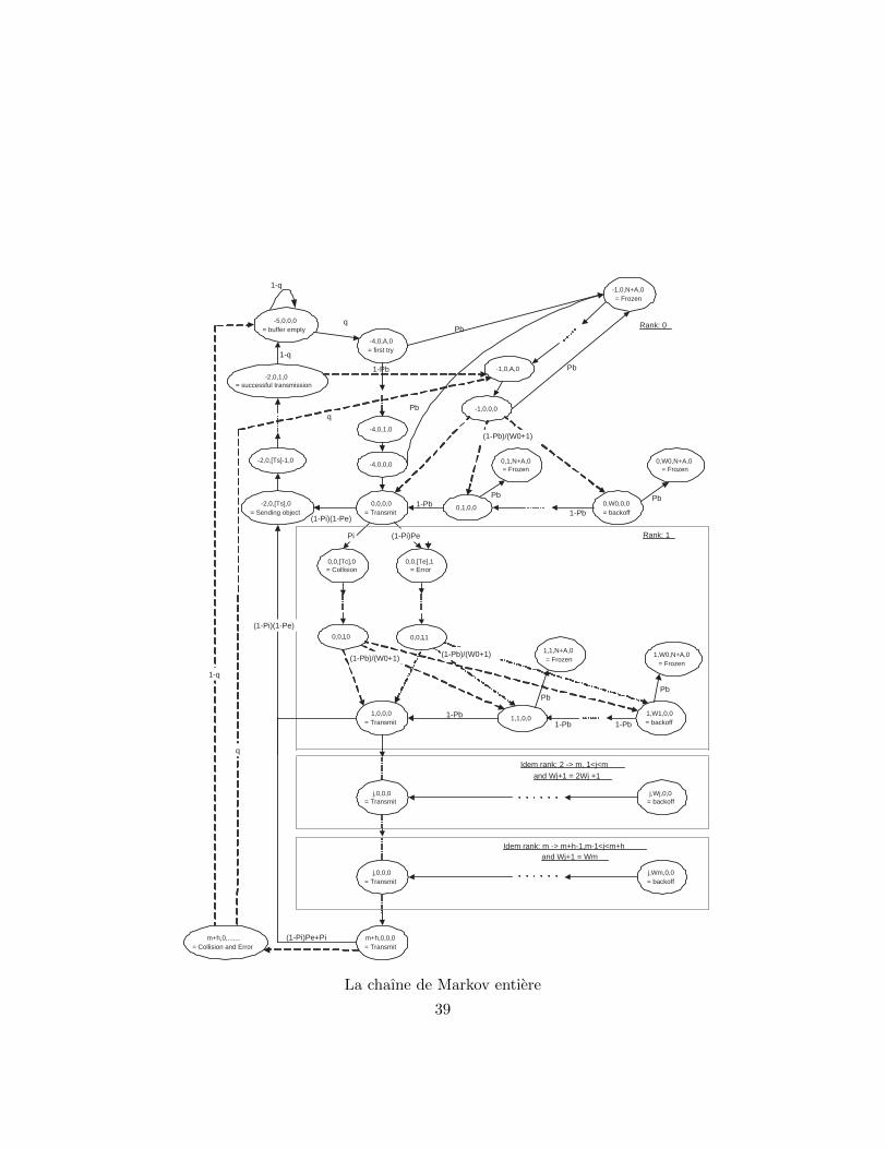
Chap 4. Modele EDCA nonsature en presence d’erreurs

La chaıne de Markov representee ci-dessous, correspond a la modelisationdu comportement d’une AC pour une STA geree par le mecanisme. Dansle cas d’une modelisation du DCF et non de l’EDCA, il suffirait dans notremodele de considerer cette chaıne comme une STA, moyennant quelquesmodifications dans les formules a venir, le principe restant exactement lememe.Nous avons introduit pour les besoins de notre modele une 4eme dimension,e(t). Cette variable binaire, indique par sa valeur a 1, lorsque la transmissionn’a pas subi de collision mais ne connaıt pas de succes car la transmissionest erronee.Cette variable a ete introduite afin de faire la difference entre, une transmis-sion echouee en raison d’une collision et celle qui echoue en raison d’une er-reur. On ne trouve pas cette dimension dans les modeles precedents puisquele canal est pour la grande majorite des modeles, suppose ideal. Dans tousles autres etats e(t) = 0.Soit pi la probabilite de collision et pb la probabilite que le canal soit occupe.Nous supposons comme [43] que ces probabilites sont independantes de laprocedure de backoff. Par ailleurs, la probabilite pi, est constituee de deuxparties : une probabilite de collision externe due aux transmissions des autresSTA et une probabilite de collision interne, due a la contention virtuelle quia lieu entre les ACi d’une meme STA.A l’instant t, on peut considerer que l’etat d’une AC est entierement deter-mine par le quadruplet (j,k,d,e) qui correspond aux valeurs prises respec-tivement par chacune des dimensions.Supposons que l’AC se trouve a l’etat (j, 1, 0, 0). L’AC a donc rencon-tre j collisions et/ou transmissions erronees et subit son jieme backoff pourtenter une retransmission du paquet en cours. Cela est indique par la pre-

37

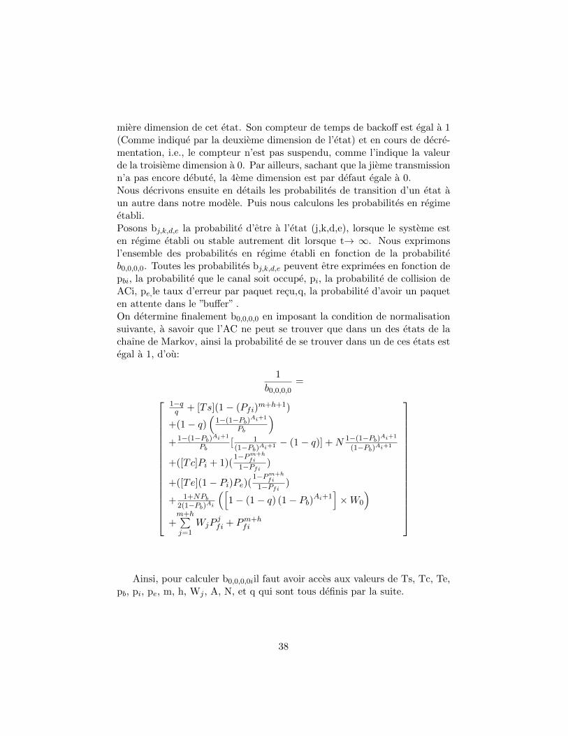
miere dimension de cet etat. Son compteur de temps de backoff est egal a 1(Comme indique par la deuxieme dimension de l’etat) et en cours de decre-mentation, i.e., le compteur n’est pas suspendu, comme l’indique la valeurde la troisieme dimension a 0. Par ailleurs, sachant que la jieme transmissionn’a pas encore debute, la 4eme dimension est par defaut egale a 0.Nous decrivons ensuite en details les probabilites de transition d’un etat aun autre dans notre modele. Puis nous calculons les probabilites en regimeetabli.Posons bj,k,d,e la probabilite d’etre a l’etat (j,k,d,e), lorsque le systeme esten regime etabli ou stable autrement dit lorsque t→ ∞. Nous exprimonsl’ensemble des probabilites en regime etabli en fonction de la probabiliteb0,0,0,0. Toutes les probabilites bj,k,d,e peuvent etre exprimees en fonction depbi, la probabilite que le canal soit occupe, pi, la probabilite de collision deACi, pe,le taux d’erreur par paquet recu,q, la probabilite d’avoir un paqueten attente dans le ”buffer” .On determine finalement b0,0,0,0 en imposant la condition de normalisationsuivante, a savoir que l’AC ne peut se trouver que dans un des etats de lachaıne de Markov, ainsi la probabilite de se trouver dans un de ces etats estegal a 1, d’ou:

1

b0,0,0,0=

1−qq + [Ts](1− (Pfi)

m+h+1)

+(1− q)(

1−(1−Pb)Ai+1

Pb

)+1−(1−Pb)Ai+1

Pb[ 1(1−Pb)Ai+1 − (1− q)] +N 1−(1−Pb)Ai+1

(1−Pb)Ai+1

+([Tc]Pi + 1)(1−Pm+h

fi

1−Pfi)

+([Te](1− Pi)Pe)(1−Pm+h

fi

1−Pfi)

+ 1+NPb

2(1−Pb)Ai

([1− (1− q) (1− Pb)Ai+1

]×W0

)+m+h∑j=1

WjPjfi + Pm+h

fi

Ainsi, pour calculer b0,0,0,0iil faut avoir acces aux valeurs de Ts, Tc, Te,pb, pi, pe, m, h, Wj , A, N, et q qui sont tous definis par la suite.

38

-5,0,0,0 = buffer empty

0,0,[Tc],0 = Collision

-1,0,0,0

0,W0,N+A,0 = Frozen

-2,0,[Ts],0 = Sending object

0,W0,0,0 = backoff

-4,0,A,0 = first try

0,0,0,0 = Transmit

-4,0,1,0

-1,0,N+A,0 = Frozen

0,1,0,0

0,1,N+A,0 = Frozen

1-q

q

1-q

Pb

1-Pb

1-Pb Pb Pb

(1-Pi)(1-Pe)

Pi

Pb

1-Pb

q

(1-Pb)/(W0+1)

0,0,[Te],1 = Error

(1-Pb)/(W0+1)

0,0, 1 ,0 0,0, 1 ,1

1,W0,N+A,0 = Frozen

1,W1,0,0 = backoff

1,1,0,0

1,1,N+A,0 = Frozen

1-Pb 1-Pb

(1-Pb)/(W0+1)

1,0,0,0 = Transmit

(1-Pi)Pe

1-Pb

Pb Pb

Rank: 1

m+h,0,0,0 = Transmit

Idem rank: 2 -> m, 1<j<m

and Wj+1 = 2Wj +1

Rank: 0

(1-Pi)(1-Pe)

1-q

q

(1-Pi)Pe+Pi

-2,0,1,0 = successful transmission

-2,0,[Ts]-1,0

-1,0,A,0

q

Idem rank: m -> m+h-1,m-1<j<m+h and Wj+1 = Wm

j,Wj,0,0 = backoff

j,Wm,0,0 = backoff

m+h,0,...,... = Collision and Error

j,0,0,0 = Transmit

j,0,0,0 = Transmit

Pb

-4,0,0,0

La chaıne de Markov entiere

39

CHAP. 5 Doublereutilisation de frequencesentre macrocell et femtocell

Dans ce chapitre nous presentons le schema d’allocations de frequences quenous proposons pour gerer les interferences entre macrocell et femtocells.Il existe de maniere generale deux approches de partages des ressources.La premiere consiste a attribuer a chaque couche a savoir macrocell etfemtocell un set de frequences dediees. En assurant un partage orthog-onal des frequences on s’assure ainsi de ne pas rencontrer des problemesd’interferences entre les deux couches. Cependant cette solution ne permetpas une utilisation efficace de la ressource.Une autre approche consiste a offrir a la seconde couche la possibilite dereutiliser la ressource deja utilisee par les macrocell. Cette solution certesoptimale induit de fortes interferences co-canal.Nous proposons un schema de reutilisation de frequences qui tire profit a lafois de la reutilisation des frequences et de l’orthogonalite entre les macrocellset femtocells.Pour cela nous nous placons dans le contexte des technologies basees surl’OFDMA. Nous proposons que chaque femtocell se trouvant dans un secteurdonne reutilise les frequences utilisees par les secteurs adjacents.Afin d’affiner ce schema de reutilisation de frequences nous proposons troisvariantes d’allocations de frequences suivant la localisation de l’appareil parrapport a la position de la station de base macrocell. Nous rappelons toutd’abord que l’on considere ici un spectre de frequences divise en trois groupesde canauxLa premiere variante surnommee ”full reuse” (reutilisation pleine) consistea offrir aux femtocells se trouvant dans un secteur donne l’ensemble descanaux des deux autres secteurs adjacents couverts par la station de base

40

macrocell.La seconde variante surnommee ”partial reuse” (reutilisation partielle) con-sidere un partage de chaque secteur en six zones triangulaires. Les femtocellsse trouvant dans chacun des triangles ne peuvent reutiliser que la partie duspectre de frequences qui n’est pas utilise par le secteur de la macrocell luifaisant face. Autrement dit, des trois groupes de frequences precedemmentdefinis, uniquement un seul d’entre eux est mis a disposition des femtocellsse trouvant dans un triangle donne. L’avantage de ce mode d’allocation estque les femtocells se trouvant dans un triangle ne souffrent pas d’interferenceprovenant du secteur faisant face au triangle. L’inconvenient est que le setde canaux disponibles pour les femtocells d’un triangle est reduit, ce qui vaforcement augmenter les interferences co-canal entre les femtocells du memetriangle.Enfin considerant que les interferences entre les femtocells mentionnees justeavant dans le cas du ”partial reuse” pourraient etre assez importantes, nousavons propose une troisieme variante. Dans ce mode surnomme ”mixedreuse” (reutilisation mixte) nous distinguons dans chaque secteur deux re-gions: la region qui borde de maniere circulaire l’ensemble du secteur surnomme”bord” et la region au centre du secteur. La region bord est a nouveau sousdivisee en zone de facon identique a la methode ”partial reuse”.La logique sous jacente a ce partage est la suivante. Comme mentionnedans le cas partial reuse, les femtocells qui bordent le secteur souffrentd’interferences co-canal severes si elles reutilisent les memes frequences queles secteurs qui leur font face. Mais d’un autre cote, restreindre les femtocellsau mode partial nous oblige a faire face a des scenarios d’interferences entrefemtocells. Ainsi comme compromis nous definissons la region bord ou lesfemtocells ne peuvent pas reutiliser les canaux utilises par les secteurs leurfaisant face. Dans la region centre le schema full reuse est applique. Ainsinous ”mixons” les deux approches precedentes.

41

Partie III : Les resultats

42

CHAP. 6 Calcul desperformances du modele del’EDCA

Les performances d’un systeme ne peuvent se resumer a une probabilite decollision. En effet, quelle utilite ces informations pourraient avoir pour unutilisateur ou un operateur?. Les informations reellement interessantes dupoint de vue de l’utilisateur correspondent aux parametres influant sur laQoS.

Le debit normalise pour une AC donnee est calcule comme le rapportentre le temps utile pour emettre les donnees et le temps moyen entredeux transmissions successives. Ce temps moyen prend en compte le tempsd’attente en procedure de contention, le temps eventuellement perdu en col-lision et/ou erreur ainsi que le temps pour emettre avec succes le paquet,incluant les differents temps d’emission des en-tetes.

Le debit Si s’exprime alors de la maniere suivante :

Si =PsiP

E[I] +∑3

i′=0 Psi′(Ts +AIFS[ACi′ ]) +∑3

i′=0 Pi′Tc + PeTe

Ou E[P] correspond a la taille des donnees utiles d’un paquet moyen.En general cette donnee est fixee pour faciliter le calcul. Cependant en pra-tique, selon l’application modelisee, cela peut s’averer inexact. Par exempleen conversation VoIP, la taille des paquets est constante et est choisie enfonction de la qualite, du delai et du codec utilises. Par contre, pour unemodelisation d’une application telle que l’affichage de pages web, la taille despaquets suit une loi assez difficile a caracteriser. De nombreuses recherchesont ete effectuees dans ce domaine, mais aucun resultat precis, n’a pu encoremodeliser correctement l’evolution de la taille des paquets pour une session

43

web. En tout etat de cause, on peut par exemple prendre une loi de poisson.La maniere de calculer E[P] est inspiree de [16].E[I] designe la valeur moyenne de time slots, inutilises, autrement dit detime slot, ou le canal est libre. Cette valeur reflete les temps de backoff.On a : E [I]= 1

pb− 1

Cette formule s’obtient en considerant une distribution geometrique de parametrepb, le temps entre 2 intervalles inutilises (idle time slot) etant obtenu par laformule ci-dessus.psi et psi′ correspondent aux probabilites que la transmission aboutisse avecsucces, pour resp. ACi et ACi’.La formule permettant d’obtenir psi est la suivante :

psi =Mpti(1− τ)M−1

∏i′>i(1− τi′)

1− (1− τ)M

avecpti = Ts ∗ (~b)i ∗ (1− (p(~τ)i)

m+h)

Pour les notations utilisees dans la formule depti, se referer plus loin a laresolution mathematique de notre probleme.Pour le calcul des temps Ts, Tc, et Te, nous avons utilise en general lesdonnees du standard.Le calcul du delai se fait de la maniere suivante. Posons Dj,k,d,e l’intervallede temps representant le delai entre le moment ou le systeme est a l’etat(j,k,d,e) et le moment ou le paquet est transmis avec succes. Le delai to-tal pour un paquet transmis avec succes correspond a l’intervalle de tempsentre le moment ou le paquet se trouve dans la file d’attente Mac, pret aetre transmis, jusqu’au moment ou la trame d’acquittement pour le paquetconcerne est recu par l’expediteur. Apres avoir effectue de nombreux cal-culs on obtient D le delai moyen qu’un paquet devra attendre, comme definiprecedemment :

D =N+A∑d=0

b−1,0,d,0D−1,0,d +M+h∑j=0

[Tc]∑d=0

bj,0,d,0Dj,0,d,0

+m+h∑j=0

[Tc]∑d=0

bj,0,d,0Dj,0,d,0 +m+h∑j=0

Wi∑k=0

N+A∑d=0

bj,k,dDj,k,d,0

44

CHAP. 7 Performances desfemtocell

Dans ce chapitre nous cherchons a determiner qu’elle serait la valeur ajouteedes femtocells si elles etaient introduites par un operateur dans son systeme.

Pour ce, nous utilisons deux metriques classiques qui sont le rapport signala Interference plus bruit (RSB) et la puissance du signal.Pour evaluer les performances selon ces metriques il a fallu tout d’abordenvisager un systeme permettant d’obtenir des resultats. Pour les besoinsde la these nous avons donc developpe un simulateur du systeme. Nouspresentons dans ce chapitre les differentes interfaces du simulateur ainsi quela maniere dont les resultats sont presentes.Par la suite nous presentons une serie de resultats de performances desfemtocells.Nous etudions tout d’abord le gain en puissance du signal recue en com-parant le cas d’un utilisateur relie a sa propre femtocell et le cas ou ce memeutilisateur est connecte a la macrocell. Nous montrons que les performancesde la femtocell sont superieures a celles de la macrocell dans tout les casmeme en supposant que la macrocell transmet a une puissance superieurede 30 dB a la puissance d’emission de la macrocell. Cela correspond au sens”descendant”. Les differences dans le sens montant sont encore plus aiguespuisque le telephone cellulaire est fortement limite en termes de puissancesd’emission independamment de la station avec laquelle il est connecte quece soit une macrocell ou femtocell.En parallele nous presentons toutes une series de resultats de rapport signala Interference plus Bruit. Cette derniere metrique est plus significative carelle prend en compte les interferences. Ainsi nous pouvons comparer lesdiverses variantes proposees.Nous montrons tout d’abord que de maniere generale le mode de pleine

45

reutilisation des frequences donne les meilleurs resultats. Ce qui s’expliqueaisement en prenant en ligne de compte les interferences entre femtocells.Dans ce mode un plus grand nombre de canaux sont mis a disposition desfemtocells.Pour pouvoir comprendre les limites des differents modes proposes nousavons etudie les performances obtenues dans des cas plus specifiques. Nousavons defini trois types de deploiements des femtocells: un deploiement uni-forme sur toute la surface du secteur, un deploiement aux bords du secteuret enfin un deploiement ou les stations sont aux centres du secteur. A notregrande surprise, nous avons decouvert que meme lorsque les stations sontsituees aux bords le mode de pleine reutilisation donne les meilleurs resul-tats. Nous en avons deduit que les interferences entre femtocells etaient bienplus significatives que celles engendrees par les macrocell adjacentes.

46

Conclusion

Apres le succes inattendu des reseaux cellulaires de 2ieme generation (2G)qui ont donne la possibilite aux utilisateurs mobiles situes en dehors deleur domicile de profiter de services de telephonie lors de leur sejour enexterieur, et le deploiement croissant de reseaux locaux sans fil a domicile,nous observons une hausse permanente de la demande en Internet mobile ahaut debit pour les utilisateurs situes en interieur..Dans cette these nous nous sommes interesses a deux technologies qui peu-vent etre definies comme des reseaux locaux sans fil: la technologie surnom-mee WiFi, et la nouvelle technologie femtocell. L’objectif de cette theseetait d’evaluer pour chacune de ces technologies separement le facteur lim-itant la possibilite d’offrir de hautes performances en termes de debits auxutilisateurs.Au niveau du WiFi, ce qui peut etre considere comme le goulot d’etranglementde la performance est le mecanisme d’acces multiples a la ressource radiopar plusieurs utilisateurs. En fait, meme si le mecanisme CSMA / CA est unbon compromis par rapport aux autres mecanismes d’acces tels que TDMA,CDMA, etc ... notamment parce qu’il est distribue, il requiert tout de memeun ensemble de temps d’attente qui entraıne un ” gaspillage ” de la ressourceradio. Le defi consistait a evaluer les performances de ce mecanisme dansles conditions les plus proches de la realite en termes de debit et de delai.En raison de la nature stochastique de ce mecanisme, les modeles theoriquessont naturellement souvent utilises afin de decrire le fonctionnement du me-canisme. Plusieurs modeles ont deja ete developpes, mais ils sont tous basessur de simples suppositions. La plupart des hypotheses communes sont entreautre celle d’un canal ideal n’introduisant aucune erreur, et celle du regimesature .... En outre les modeles existants ne considerent pas le mecanisme dela couche MAC du WiFi qui offre une differenciation des services autrementdit le support de la qualite de service (en anglais QoS: Quality Of Service).Dans la premiere partie de cette these nous avons developpe un modele

precis du mecanisme EDCA se basant sur une chaıne de Markov a quatre

47

dimensions. Ce modele est une extension du modele de Kong et al, lui memebase sur le modele original de Bianchi. Nous avons modifie ce modele pour yinclure un canal non ideal ou des erreurs peuvent se produire avec une proba-bilite fixe. Nous considerons egalement differents scenarios de trafic: saturesou non satures avec des charges de trafic variables. Grace a notre modele,nous avons pu analyser l’effet des differents parametres du mecanisme EDCAsur le debit tels que la fenetre de contention ”Contention Window” ou lestemps d’attentes entre trame AIFS qui permettent de differencier les utilisa-teurs. Nous montrons que ces parametres offrent une bonne differenciationentre les categories d’acces des differents services. Nous montrons aussi lesdelais subis par les utilisateurs pour chaque categorie d’acces. Nous obser-vons que le facteur q de non-saturation a un effet non negligeable sur le delaice qui confirme a nouveau l’importance d’un modele non sature du reseau.Ainsi, notre modele est tres riche, ce qui le rend plus precis et plus prochede la realite, mais qui necessite des calculs plus complexes. Le resultat prin-cipal du modele consiste en calcul du debit qui conduit a l’evaluation de lacapacite du systeme. Ce resultat est essentiel pour concevoir un outil dedeploiement de reseaux de type WiFi. Notre non-modele non-sature permetd’eviter un surdimensionnement qui conduirait a de fortes interferences entredifferents points d’acces etant donne le nombre restreint de canaux utilis-ables dans cette technologie.Dans la deuxieme partie de cette these, nousavons evalue les performances des femtocell. Nous avons d’abord presenteles defis et les opportunites de cette nouvelle technologie. Ensuite, nous noussommes focalises sur le principal facteur limitant la performance a savoir lesinterferences co-canal.Ce defi est directement lie a la facon dont nous allouons les ressources radioa ce reseau seconde couche. Dun cote si nous divisons le spectre communpartage entre les macrocells et la couche femtocell en deux spectres disjointsnous beneficions d’une protection contre les interferences co-canal. Cepen-dant l’efficacite du spectre est perdue. D’un autre cote si nous laissons auxdeux couches la possibilite de partager le spectre nous sommes confrontes aun scenario de fortes interferences .Dans un premier temps nous avons presente un schema d’allocation desressources radio deja existant. Nous avons constate que beaucoup de meth-odes deja existantes depuis longtemps ont ete deja proposees au moment oules Femtocell ont ete envisages pour les technologies de deuxieme generation(2G) comme par exemple le GSM. Toutefois, le concept de femtocell n’avaitpas ete serieusement considere a ce moment.Ensuite, nous avons propose un nouveau schema de reutilisation des frequencesqui permet de melanger les deux approches mentionnees, a savoir le fraction-

48

nement du spectre et le partage du spectre. Afin d’accroıtre l’efficacite del’utilisation de la ressource radio, nous avons propose de reutiliser les canauxalloues au secteur voisin de la macrocell se superposant actuellement a lafemtocell. Trois formes de reutilisation differentes ont ete proposees, cha-cune adaptee a un scenario specifique. Nous avons fonde notre systeme derepartition sur des systemes deja existants, mais qui ont ete proposes dans lecadre de Microcell ou d’autres technologies. Nous avons suppose que la tech-nologie sous-jacente est basee sur l’OFDMA qui permet de diviser le spectre.Ainsi, notre systeme ne peut pas etre applique au reseau 3G, si l’operateurne possede qu’une seule bande de frequences. Dans le cadre de cette thesenous avons developpe un simulateur statique du systeme qui nous permetd’obtenir les performances realisees par les femtocell lorsque notre systemede repartition est utilise. Les metriques utilises furent le RSS (puissancedu signal recu) et SINR (rapport de signal a interference et bruit). Nousmontrons que femtocell surpasse en termes de performances les macrocellsdans toutes les configurations, meme lorsque la macrocell transmet a unepuissance relativement elevee.En conclusion, peut-on repondre a la question: quelle est la meilleure tech-nologie?. Malheureusement nous ne sommes pas en mesure de declarer levainqueur. Tout d’abord peut-etre qu’il n’y a pas de gagnant. Parce quechaque technologie offre une qualite de service different selon qu’il s’agissede services donnes ou de voix.

Mais pour etre en mesure d’examiner la meilleure technologie, meme pourun service donne, nous avons a faire face a des problemes supplementaires.Par exemple, nous devons considerer les performances bout a bout. En effet,tant les femtocells que le WiFi sont rattachees aux reseaux de l’operateurpar le biais de la connexion a large bande fixe de l’utilisateur par exemplel’ADSL.

Cependant la difference est que pour la femtocell, une fois la passerelle(Gateway) de l’operateur atteint, une ressource dediee est utilisee tandis queles paquets WiFi sont achemines par le reseau internet classique avec tousles delais que cela induit tels : les congestions de reseaux etc. . . .

Ainsi, certes le WiFi peut offrir des debits plus eleves, surtout si l’onconsidere l’emergence du standard 802.11 ”n”. Mais le delai requis peut nepas convenir pour des applications sensibles aux retards tels que les appli-cations de telephonie. En outre, certains avantages doivent etre traduitsdirectement en termes de performance. Par exemple, l’un des principauxavantages de la femtocell est qu’elle permet l’utilisation du meme telephonemobile deja achete, alors qu’un appareil surnomme ”dual-mode” est neces-saire si nous voulons que notre telephone mobile se connecte aux reseaux

49

wifi. C’est pourquoi une etude approfondie qui inclurait des parametreseconomiques serait necessaire. Il faudrait aussi prendre en compte pour lesfemtocells les economies realisees par l’operateur et l’utilisateur.

50

Chapter 1

Introduction

1.1 ”Ubiquitous Wireless”

Introduction of smartphones (Blackberry, iPhone and more recently theiPad), lead us to a new era where data is accessible ”anywhere”, and ”any-time”. More than 10 years after the extraordinary success of the wired in-ternet, we are experiencing a new explosion of wireless internet which is thelogical continuation of the new needs created by the Internet. The possibili-ties offered by the Internet in terms of communications(Skype, ICQ, Gmail,...), information(Wikipedia, ...), exchange (e-commerce ,...) and others hasbecome ”too” ever-present in our daily lives to be confined to a wire thatcan be plugged in only certain places. But the appeal of wireless is notwithout challenges. Wireless communications is inherently different thanwireline with many physical impairments that apply only to wireless chan-nels. Despite these, the appeal of wireless is so great that shortly after theappearance of wired data networks in the 60s (ARPANET etc. ..), protocolsdesigned for wireless networks were considered (ALOHA by N. Abramsonin 1970 [9]). It is nearly 25 years since the first mobile phone appeared. Inthose early years of wireless the primary use considered was voice service.Short messaging service ”SMS”included in the first Global System for Mobilecommunication (GSM) standard from the early 90’s experienced a successwell beyond the expectation of its designers. Then, there was the evolutionto wireless data services with General Packet Radio Service (GPRS), Uni-versal Mobile Telecommunication System (UMTS) and High Speed PacketAccess (HSPA). Accessibility to broadband data services from a fixed ter-minal took off with the emergence of the Wireless Fidelity (WiFi) standardin 1997. From that time, many additional wireless standards have been de-

51

veloped such as Bluetooth for short-range and low throughput, Ultra WideBand (UWB) for High Speed data rates, and Wireless Interoperability forMicrowave Access (WiMAX) for long range. Unlike the cellular technology,these standards are mainly intended to support delay tolerant data services(e.g. mail, web, FTP etc ...). These two groups of technologies namelythose intended for cellular services and those for fixed data services havemerged over the years to offer high data rates even for mobile; what will besubsequently dubbed: fixed mobile convergence.

One year ago, the mobile world celebrated its four billionth connection[38]. Meanwhile Third Generation (3G)-based cellular networks continue tobe deployed and 3.5G is already on the horizon. For the end user, it meansthat new and better services will become available. However, the problems ofcoverage and capacity are still open. These problems are even more severefor indoor users where reception is poor. Improvements in service to theindoor user should be meaningful especially when several surveys show thatindoor traffic can reach more than 30 percent of the total access traffic [69].

At the same time, wireless local area networks such as WiFi are almostubiquitous in most homes. WiFi users who purchased a dual-mode mobilephone, once arriving at home switch to their local wireless connection, andmake free calls through Voice over IP software. Cellular operators interestedin keeping their clients’ loyalty have to find a competitive alternative. One ofthe most promising solutions is the deployment of femtocells. A femtocell isa box quite similar in appearance to the classical WiFi router and is pluggedto the home’s broadband network access for the internet. This technologyis being tested worldwide by manufacturers and operators and might be atechnology that will help cellular network operators.

1.2 Challenges

What technology to choose to achieve good indoor coverage, and the re-quired data services?. There was a time when as mentioned above eachtechnology corresponded to a specific service. This is no longer true. Weneed to understand in greater depth the capabilities of each of these tech-nologies. For some wired technologies, simple calculations enable ”rough”approximations. This is not the case for wireless, where the radio resourcesare shared. Whatever the considered multiple-access protocol, we must takeinto account the interference that might occur between or within the tech-nology . Moreover even if one considered only a hypothetical cell ”isolatedfrom the rest of the world”, one would consider the bandwidth ”wasted” by

52

the multiple access protocol. In this present work we propose to evaluatethe capabilities of two technologies: WiFi and femtocell. The difficulty ofassessment for each of these technologies is not at the same level.

1.2.1 Capacity Evaluation of a Wifi Cell

For the WiFi, the major problem is to get the residual and effective through-put a user can expect from its wireless access point. The WiFi standardis based on the well-known Carrier Sense Multiple Access with CollisionAvoidance (CSMA / CA) mechanism which manages the multiple access toan access point by different users. This is in done in a distributed manner.Each user must verify that the channel is free during a given amount oftime (called Inter-Frame Space (IFS)) before transmitting. If the channel isbusy, the user must wait again for a random time (known as Backoff time)to try a retransmission. Even when a station succeeds to transmit on achannel that is supposed ”free”, a collision can still occur. For example, iftwo stations connected to the same access point have by coincidence waitedthe same random time. This stochastic nature of the mechanism makes itdifficult to get an accurate estimate of the actual capacity of the wirelesscell. One could argue that if we do not want to take a risk, it is enough tooversize the network by introducing a large number of wireless access pointsto cover a given area. Unfortunately, this solution feasible at high cost withwire can lead to strong interferences between cells in wireless. In addition tothe extent that CSMA / CA is used, the problem of the Exposed node willappear very quickly with an abundance of access points. Thus it is essentialto evaluate precisely and accurately as possible the capacity of a wirelesscell, in order to optimize the use of the radio resource available for eachaccess point.

1.2.2 Qos Parameters for WiFi

The original access mechanism of the WiFi standard, based on CSMA /CA was not designed initially to support quality of service. Thus there wasno differentiation mechanism between flows from different kinds of services.This motivated the development of an amendment to the original standardwhich allows giving priority to certain types of flows (e.g. for voice services,streaming, etc). Unfortunately it required the introduction of different back-off times for each flow, which complicates the task of evaluation of the cellcapacity. In addition, there are numerous parameters available within theQuality of Service (QoS) enhanced protocol that allow a network administra-

53

tor to dynamically manage the differentiation between the services. Howeverdue to the high complexity of the protocol and its random nature, it is notpossible at first sight to define the influence of each parameter on the ef-fective capacity available to each service. This evaluation can only be donethrough incremental simulations or analytical models.

1.3 Thesis Goals and Contributions

1.3.1 Stochastic Model for Wifi Access

To evaluate the capacity of a WiFi cell, a way to model the access mechanismof the radio resource was needed. Many models appeared shortly after theappearance of the standard. However, each model made some assumptionsfor purposes of simplification. The most common assumptions were thesaturation of the channel and the approximation of an ideal channel. Thechannel can be considered saturated if a user always has a packet to transmit,or in other words that the buffer of the user is never empty. This assumptionis often justified as it can be considered the worst case scenario which willnot lead to overestimated capacity. However, this will obviously lead to anoversized network which is not desirable. In addition, this assumption isitself difficult to justify if we consider that a user rarely has a packet totransmit continuously. For instance, the traffic of a user viewing web pageshas been the subject of intense research and often modeled for simplicityhas a series of burst period followed by silence period maybe due to thefact that the user takes time to read the required information that has beendownloaded and does not interact continuously. A second approximationoften assumed in the existing models considers the channel as ideal. Thus,each transmitted packet arrives without error with a probability equal to 1 ifit does not encounter a collision. It is well known that the wireless mediumis far from being error free. If for the wired network, the BER is around10−14, wireless networks have a BER of around 10−7 or about 10 milliontimes more errors. So once again we claim that this is a rough assumption.Finally, many models do not consider the enhanced access mechanism of theWiFi which supports QoS.

In this thesis we propose to model the access mechanism of a WiFi’scell with QoS support and without the aforementioned approximations ofsaturation and error-free channel. Indeed we consider the possibility thatthe buffer of the user can be empty with a given probability. Moreover, evenif the user was granted access to the medium, there is non zero probabil-ity that an error occurs. For theses purposes we extend an existing model

54

known as Bianchi’s model [16] which was further extended to accommodatethe QoS enhancement by Kong [48]. The new model allows for more accu-rate dimensioning of a WiFi network. Moreover, the modeling of the QoSstandard capability allows a better understanding of the influence of eachparameter of the protocol. Thus our model may be considered as a tool forcalibrating parameters of the network to give specific quality of service todifferent users.

1.3.2 Femtocell

The difficulty for the femtocell lies at another level. In fact the multipleaccess mechanism considered is, according to the generation: Code DivisionMultiple Access (CDMA) for 3G and Orthogonal Frequency Division Mul-tiple Access (OFDMA) for 4G. These mechanisms are not stochastic, thusevaluation of the capacity for a cell is not really challenging. On the otherhand if we take into account the neighboring cells, then we have to dealwith interference scenarios. In addition, unlike WiFi, femtocells must con-sider the overlay macrocell. Indeed although femtocells allow better coverageinside, we still have to provide coverage for outside users not connected to afemtocell. This additional coverage overlays the femtocell like an umbrella.Therefore we have to face a new challenge which is spectrum allocation to thefemtocell. It is now well known that radio resources are rare ”commodities”.If the femtocell reuses the spectrum already allocated to the macrocell thiswill necessarily induce strong interference between femtocell and macrocell,even if it seems to be an appealing proposal in terms of optimization. Ded-icated spectrum for femtocell is not always possible if the operator does nothave additional spectrum for this second layer of mini-base stations. Thusin order to evaluate the capability of a femtocell, we have to cope first withspectrum allocation.

In this thesis we propose an innovative scheme for frequency reuse be-tween femtocells and macrocells. We propose to merge the two approachesmentioned above. Namely, we grant femtocell spectrum which would consistof dedicated frequencies from adjacent sectors of the overlaying macrocell.At the time we developed this idea there was still no methods of optimalsharing of frequencies between femtocells and macrocells. After grantingthe femtocell a spectrum, we can then consider the calculation of the fem-tocell capability in terms of signal to noise ratio achievable and thereforedata rates. This calculation takes into account the interference generatedby neighboring femtocells reusing the same frequencies, called co-channelinterference, as well as those generated by users of the macrocell still on

55

camping on the same frequencies. Our contribution is manifold. Mobileoperators will be able to optimize the use of the radio resource acquired.On the other hand we allow to evaluate the added value of a complemen-tary coverage by femtocells, both from a femtocell user and macrocell userperspective.

1.4 Thesis Outline

This thesis has a somewhat original structure to the extent that we dealwith two parallel competing technologies. The objective being to assessthe capacity offered by each. We propose to deal in parallel with each ofthese challenges. The first part presents the technical background for a goodunderstanding of the challenges and their solutions. Then, a thorough treat-ment of the state of the art for each issue is given. Due to the specificity ofeach technology each is presented in separate chapters. Chapter 2 shows thebackground and already existing works for dimensioning of a wireless cell.Chapter 3 presents the challenges to be overcome with femtocells and thevarious existing solutions already proposed. This parallelism is maintaineduntil the end of the thesis. The second part presents our contribution to eachof these issues in details. In Chapter 4 we present the stochastic model de-veloped to fill the need for an accurate evaluation of the capability of a WiFicell. Then in chapter 5 we present our scheme for double frequency reusebetween femtocell and macrocell. The third part of this thesis presents theresults from each of the proposed solutions. Chapter 6 reports the differentperformance achievements in terms of effective throughput and delay for asingle cell under different load scenarios, probabilities of error etc. Chapter7 presents the potential of femtocells mainly in terms of signal to noise ratiothat can be achieved thanks to our reuse scheme. This thesis concludes witha brief comparison between the two technologies and some ideas for futureworks.

56

Part I

Background and state of theART

57

In this part, we present the required background to understand howWiFi and femtocell technologies work. In the following chapter we presentthe access mechanism to the IEEE 802.11(a.k.a WiFi) radio interface. Mod-eling of WiFi’s Medium Access Control (MAC) layer function has drawn theattention of hundreds of researchers throughout the world and will be there-fore thoroughly detailed in Section 2.2. We further introduce the concept offemtocell in Chapter 3, with the challenges and existing work relative to theradio resources allocation issue. In the next part we present our contributionto all these problems with respect to the state of the art.

58

Chapter 2

Access Mechanisms to IEEE802.11 WiFi Networks andTheir Analytical Model

This chapter presents the mechanism of multiple access used in the WirelessLocal Area Network (LAN) (WLAN) following the IEEE 802.11 standard.Then we provide a deep insight through the state of the art on this topic.

2.1 MAC of the IEEE 802.11 and 802.11e descrip-tion

In the last years , WiFi products enjoy more and more interest from theconsumer and therefore bring to the libraries quantities of literature on itsmechanism. This chapter is an overview of the main concepts of WiFi fol-lowed by details of the MAC layer according to the original 1997 standard.Then the QoS amendment to the standard is explained.

2.1.1 introduction

The IEEE 802.11 standard (ISO / IEC 8802-11) is an international stan-dard describing the characteristics of a WLAN-Wireless Local Area Network(WLAN) [1] . The name Wi-Fi (contraction of Wireless Fidelity , and oftendenoted WiFi) is originally the name given to the certification allocated bythe Wi-Fi Alliance, formerly WECA (Wireless Ethernet Compatibility Al-liance), the body responsible for maintaining the interoperability betweenequipment meeting the 802.11 standard. WiFi allows broadband WLAN if

59

the station is not too far from the access point.The 802.11 standard definestwo modes of operation [6]: infrastructure mode and ad hoc mode. In in-frastructure mode, the wireless network has at least one access point (AP)connected to the wired network infrastructure and a set of wireless stations ,whereas in ad-hoc mode, there is no AP but only set of Stations (STAs) thatcommunicate directly with each other. The IEEE 802.11 standard definesonly the two first layers of the OSI model: the Physical Layer (PHY)and theMAC(medium access control layer). The PHY layer defines how to transmitthe bits on the physical medium including which modulation etc.. The MAClayer deals with scheduling of the user data into packets and then into themedium. In the next sections the core mechanism of the MAC will be de-scribed since our main contributions lie in the modeling of these mechanisms.Several nominal data rates can be achieved with the WiFi technology. Itdepends on the version of the standard used. The original version referred toas IEEE 802.11b uses the Direct Sequence- Spread Spectrum (DS-SS) tech-nology which allows rates up to 11 Mbps in the ISM band. Later, a versionbased on Orthogonal Frequency Division Multiplexing (OFDM) technologywas defined in the 5 Ghz band, which allows data rates up to 54 Mbps. Thisis referred to as IEEE802.11a. Finally, due to the success of the ISM band,an upgrade of the IEEE 802.11b, was defined in the ISM radio band butwith the OFDM technology too, known as IEEE 802.11g. It allows datarates up to 54 Mbps but also compatible with the ”b” version.

Since a WLAN relies on a common transmission medium, the transmis-sions of the network stations must be coordinated by the medium accesscontrol (MAC) protocol.MAC protocols for LANs can be roughly catego-rized into : random access (e.g., CSMA, Carrier Sense Multiple Access withCollision Detection (CSMA/CD)) and demand assignment (e.g., token ring).Due to the inherent flexibility of random access systems (e.g., random ac-cess allows unconstrained movement of mobile hosts) the IEEE 802.11 stan-dard committee decided to adopt a random access CSMA-based scheme forWLANs[19]. The IEEE 802.11 MAC sub-layer defines two relative mediumaccess coordination functions, the Distributed (Coordination Function) In-terframe Space (DCF)) which is a contention mode and the optional PointCoordination Function (PCF) which is a contention free mode. The PCFmechanism was optionally from the beginning and was never implementedin a commercial product.Therefore, we will not consider it further.

60

2.1.2 Distributed Coordination Function

DCF is a distributed medium access scheme. In this mode, a station mustsense the medium before initiating a packet transmission [56]. If the mediumis found idle for a time interval longer than Distributed InterFrame Space(DIFS), then the station can transmit the packet directly. Otherwise, thetransmission is deferred and the backoff process is started Fig.2.1. Specif-ically, the station computes a random time interval named Backoff time,uniformly distributed between zero and the current Contention Window size(CW), Backoff time = rand[0;CW ], where CWmin < CW < CWmax andSlot time depends on the PHY layer type. The backoff timer is decreasedonly when the medium is idle, whereas it is frozen when another stationis transmitting. Each time the medium becomes idle, the station waits fora DIFS and then continuously decrements the backoff timer. As soon asthe backoff timer expires, the station is authorized to access the medium.Obviously, a collision occurs if two or more stations start transmission si-multaneously. In this scheme there is no collision detection capability dueto the WLANs inability to listen while sending, since there is usually justone antenna for both sending and receiving and due due to the significantdifference between transmitted and received power levels. Hence, a positiveacknowledgement is used to notify the sender that the transmitted framehas been successfully received. The transmission of the acknowledgementis initiated at a time interval equal to the Short InterFrame Space (SIFS)after the end of the reception of the previous frame see fig 2.2. Since theSIFS is smaller than the DIFS see fig. 2.1, the receiving station does notneed to sense the medium before transmitting an acknowledgement. If theacknowledgement is not received, the sender assumes that the transmittedframe was lost and schedules a retransmission and then enters the backoffprocess again. To reduce the probability of collisions, after each unsuccessfultransmission attempt, the contention window is doubled until a predefinedmaximum value CWmax is reached. To improve the channel utilization, af-ter each successful transmission, the contention window is reset to a fixedminimum value CWmin.

The Network Allocation Vector (NAV) is used for MAC virtual carriersensing, by updating the local NAV with the value of other stations’ trans-mission duration. By using NAV, a station can know when the currenttransmission ends and channel is idle. In order to solve the so-called hiddenterminal problem, an optional RTSRequest To Send (RTS)/Clear To Send(CTS) (RequestToSend and ClearToSend) scheme is introduced, see Figure2.3. The transmitter sends a short RTS frame (20 bytes) before each data

61

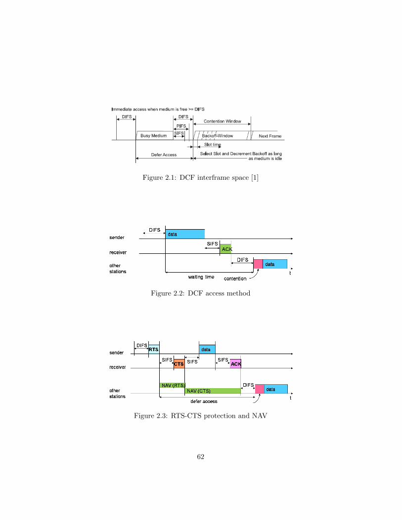
Figure 2.1: DCF interframe space [1]

Figure 2.2: DCF access method

Figure 2.3: RTS-CTS protection and NAV

62

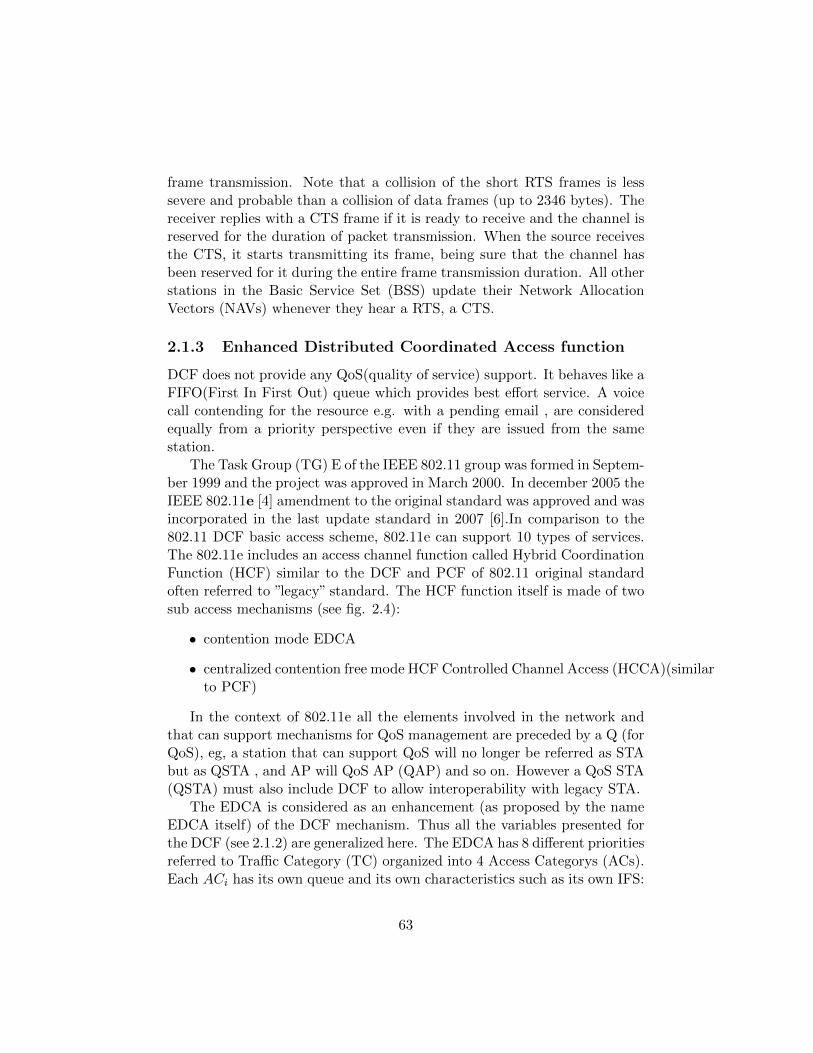
frame transmission. Note that a collision of the short RTS frames is lesssevere and probable than a collision of data frames (up to 2346 bytes). Thereceiver replies with a CTS frame if it is ready to receive and the channel isreserved for the duration of packet transmission. When the source receivesthe CTS, it starts transmitting its frame, being sure that the channel hasbeen reserved for it during the entire frame transmission duration. All otherstations in the Basic Service Set (BSS) update their Network AllocationVectors (NAVs) whenever they hear a RTS, a CTS.

2.1.3 Enhanced Distributed Coordinated Access function

DCF does not provide any QoS(quality of service) support. It behaves like aFIFO(First In First Out) queue which provides best effort service. A voicecall contending for the resource e.g. with a pending email , are consideredequally from a priority perspective even if they are issued from the samestation.

The Task Group (TG) E of the IEEE 802.11 group was formed in Septem-ber 1999 and the project was approved in March 2000. In december 2005 theIEEE 802.11e [4] amendment to the original standard was approved and wasincorporated in the last update standard in 2007 [6].In comparison to the802.11 DCF basic access scheme, 802.11e can support 10 types of services.The 802.11e includes an access channel function called Hybrid CoordinationFunction (HCF) similar to the DCF and PCF of 802.11 original standardoften referred to ”legacy” standard. The HCF function itself is made of twosub access mechanisms (see fig. 2.4):

• contention mode EDCA

• centralized contention free mode HCF Controlled Channel Access (HCCA)(similarto PCF)

In the context of 802.11e all the elements involved in the network andthat can support mechanisms for QoS management are preceded by a Q (forQoS), eg, a station that can support QoS will no longer be referred as STAbut as QSTA , and AP will QoS AP (QAP) and so on. However a QoS STA(QSTA) must also include DCF to allow interoperability with legacy STA.

The EDCA is considered as an enhancement (as proposed by the nameEDCA itself) of the DCF mechanism. Thus all the variables presented forthe DCF (see 2.1.2) are generalized here. The EDCA has 8 different prioritiesreferred to Traffic Category (TC) organized into 4 Access Categorys (ACs).Each ACi has its own queue and its own characteristics such as its own IFS:

63

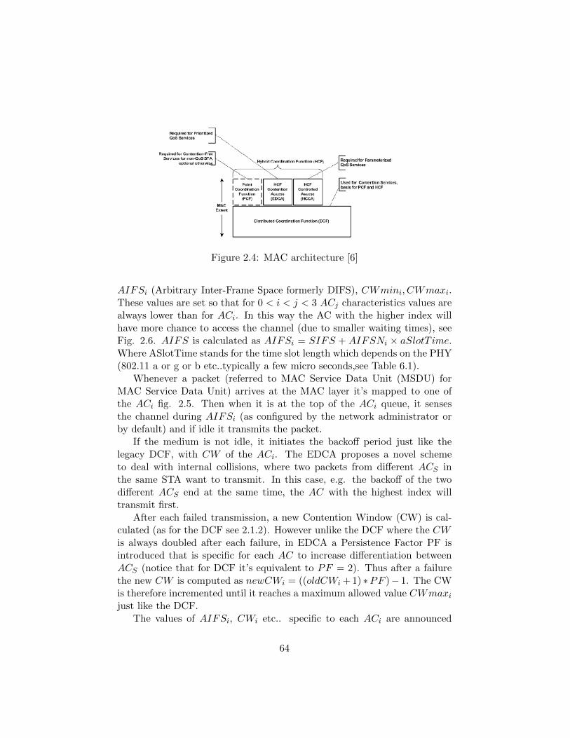
Figure 2.4: MAC architecture [6]

AIFSi (Arbitrary Inter-Frame Space formerly DIFS), CWmini, CWmaxi.These values are set so that for 0 < i < j < 3 ACj characteristics values arealways lower than for ACi. In this way the AC with the higher index willhave more chance to access the channel (due to smaller waiting times), seeFig. 2.6. AIFS is calculated as AIFSi = SIFS + AIFSNi × aSlotT ime.Where ASlotTime stands for the time slot length which depends on the PHY(802.11 a or g or b etc..typically a few micro seconds,see Table 6.1).

Whenever a packet (referred to MAC Service Data Unit (MSDU) forMAC Service Data Unit) arrives at the MAC layer it’s mapped to one ofthe ACi fig. 2.5. Then when it is at the top of the ACi queue, it sensesthe channel during AIFSi (as configured by the network administrator orby default) and if idle it transmits the packet.

If the medium is not idle, it initiates the backoff period just like thelegacy DCF, with CW of the ACi. The EDCA proposes a novel schemeto deal with internal collisions, where two packets from different ACS inthe same STA want to transmit. In this case, e.g. the backoff of the twodifferent ACS end at the same time, the AC with the highest index willtransmit first.

After each failed transmission, a new Contention Window (CW) is cal-culated (as for the DCF see 2.1.2). However unlike the DCF where the CWis always doubled after each failure, in EDCA a Persistence Factor PF isintroduced that is specific for each AC to increase differentiation betweenACS (notice that for DCF it’s equivalent to PF = 2). Thus after a failurethe new CW is computed as newCWi = ((oldCWi + 1) ∗PF )− 1. The CWis therefore incremented until it reaches a maximum allowed value CWmaxijust like the DCF.

The values of AIFSi, CWi etc.. specific to each ACi are announced

64

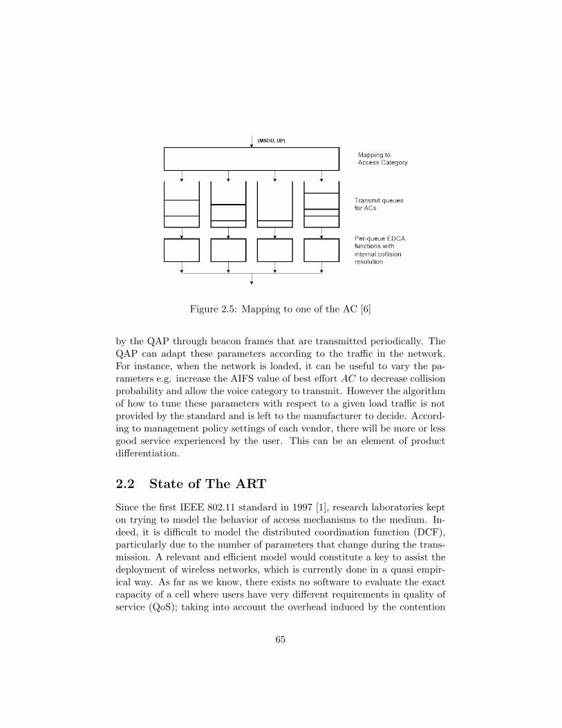
Figure 2.5: Mapping to one of the AC [6]

by the QAP through beacon frames that are transmitted periodically. TheQAP can adapt these parameters according to the traffic in the network.For instance, when the network is loaded, it can be useful to vary the pa-rameters e.g. increase the AIFS value of best effort AC to decrease collisionprobability and allow the voice category to transmit. However the algorithmof how to tune these parameters with respect to a given load traffic is notprovided by the standard and is left to the manufacturer to decide. Accord-ing to management policy settings of each vendor, there will be more or lessgood service experienced by the user. This can be an element of productdifferentiation.

2.2 State of The ART

Since the first IEEE 802.11 standard in 1997 [1], research laboratories kepton trying to model the behavior of access mechanisms to the medium. In-deed, it is difficult to model the distributed coordination function (DCF),particularly due to the number of parameters that change during the trans-mission. A relevant and efficient model would constitute a key to assist thedeployment of wireless networks, which is currently done in a quasi empir-ical way. As far as we know, there exists no software to evaluate the exactcapacity of a cell where users have very different requirements in quality ofservice (QoS); taking into account the overhead induced by the contention

65

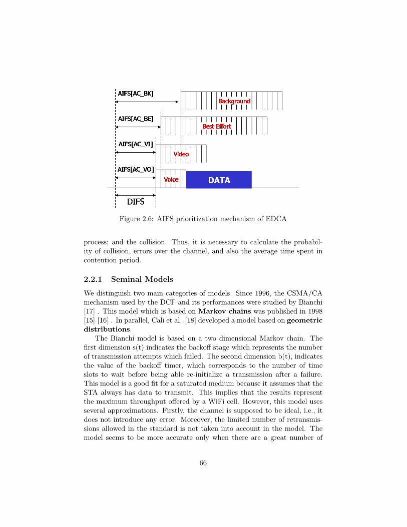
Figure 2.6: AIFS prioritization mechanism of EDCA

process; and the collision. Thus, it is necessary to calculate the probabil-ity of collision, errors over the channel, and also the average time spent incontention period.

2.2.1 Seminal Models

We distinguish two main categories of models. Since 1996, the CSMA/CAmechanism used by the DCF and its performances were studied by Bianchi[17] . This model which is based on Markov chains was published in 1998[15]-[16] . In parallel, Cali et al. [18] developed a model based on geometricdistributions.

The Bianchi model is based on a two dimensional Markov chain. Thefirst dimension s(t) indicates the backoff stage which represents the numberof transmission attempts which failed. The second dimension b(t), indicatesthe value of the backoff timer, which corresponds to the number of timeslots to wait before being able re-initialize a transmission after a failure.This model is a good fit for a saturated medium because it assumes that theSTA always has data to transmit. This implies that the results representthe maximum throughput offered by a WiFi cell. However, this model usesseveral approximations. Firstly, the channel is supposed to be ideal, i.e., itdoes not introduce any error. Moreover, the limited number of retransmis-sions allowed in the standard is not taken into account in the model. Themodel seems to be more accurate only when there are a great number of

66

stations. Besides delay is not derived.Cali’s model also allows to compute the maximum flow offered in sat-

urated mode for the DCF, but this time, the backoff time is evaluated asthe average of a geometric distribution. Although both Cali’s and Bianchi’smodels use the same approximations,a major difference between those twomodels lies in the way of computing the probability for a station transmittingat a time t (the computation being easier in Cali’s model).

2.2.2 DCF models

In order to enrich these two models, several papers were published that triedto improve one of the approximations listed previously.

[72] developed a model with an error-prone channel based on Cali’smodel. We notice that the maximum attempt of retransmissions is nottaken into account. This model leads to a finite load of the network, thusit can be considered as a non saturated model. It is based on geometricdistribution [73] and relies essentially on the work of Tobagi [65] who usedmatrices to represent the state variations of the network. Each node of thenetwork is in a ”thinking” state if it’s either waiting for a packet to transmitor has already succeed to transmit a packet in the first attempt. Other-wise the node is in ”backlogged” state where the packet is still waiting inthe buffer or being transmitted by the station. The matrices account forthe transition probabilities from a system of i backlogged nodes and M − ithinking nodes to k and M − k respectively.

Several improvements of Bianchi’s model have also been proposed. Amongthe refinements, one is due to [75] aiming to capture the freezing of backoffcounters when the broadcast channel is sensed busy by a station. How-ever an inaccuracy in the model affecting several important measures wasreported later, and corrected in [32]. [22] derives the delay but still in thesaturated mode with ideal channel assumptions. The assumptions is thatthe average backoff time that a station wait in the contention period equalto half of the contention windows, in the same way of Cali [18]. However theprobability that a station transmit is derived in the same way as Bianchi[15] which leads us to consider this model as an extention of the Bianchi’smodel. [29] improves Bianchi’s model by taking into account an error pronechannel, but still with the saturation assumption. The error probability isnot integrated in the markov chain but directly in the calculation of thecollision probability.

[20] examined unsaturated networks, by introducing an additional stateinto the Markov chain. This state takes into account the possibility of having

67

an empty buffer after a transmission. The model deals with an additionalproblem, which is that of the multi-rate STA. It is achieved by taking intoaccount the rate of each of the stations in the derivation of the transmissiontime of data. However, this work was carried out within the framework ofan ideal channel, and does not take into account several significant charac-teristics of the DCF such as the frozen time when the channel is busy.It ’sworth to mention that the model was compared against real measurementsfrom a 802.11b testbed developed for this purpose. A similar treatment offinite load can be found also in [10].

Some other models were used to derive performance of the DCF. Forexample we can mention [40] based on stochastic peri nets.

2.2.3 EDCA models

The IEEE 802.11e standard [4] including mechanisms for QoS management,has also been studied, in saturated mode [48], [57], [30], [55].These modelsare both based on Markov chains and extend the Bianchi’s model. Theyassume that the system is in saturated mode and that the channel is ideal.It’s worth to remind that all the mentioned models including our modelpresented further deal only with the infrastructure mode of the IEEE 802.11(i.e. single hop). Ad-hoc mode or multi-hop is not considered. [49] alsoextends the Bianchi’s model but without introducing a new state in theMarkov chain. Instead, it deals with the multiple access categories directlyin the computation of the collision probability.

In [13], a model to analyze the delay behavior of the EDCA mechanismis presented. The collision probability is computed with the assumption ofCali’s model [19] that backoff times follow a geometric distribution. Delayderivation following the Bianchi’s model is computed in [14] and is a directextension of [55].

An interesting approach is found in [42], which presents a unified modelbased on three different seminal models [15],[18],[64].( the two first were ex-plained in 2.2.1). Backoff stages are still accounted for by using a bidimensional-state Markov Chain as in [16] but in order to account for the effect of dif-ferent AIFS values, we did not introduce further dimension(s) to the statespace. Instead they used multiple bidimensional chains which easier to ap-ply beacuse reducing the complexity of Markov chains, what the authorsclaimed.

2.2.4 Summary Table

68

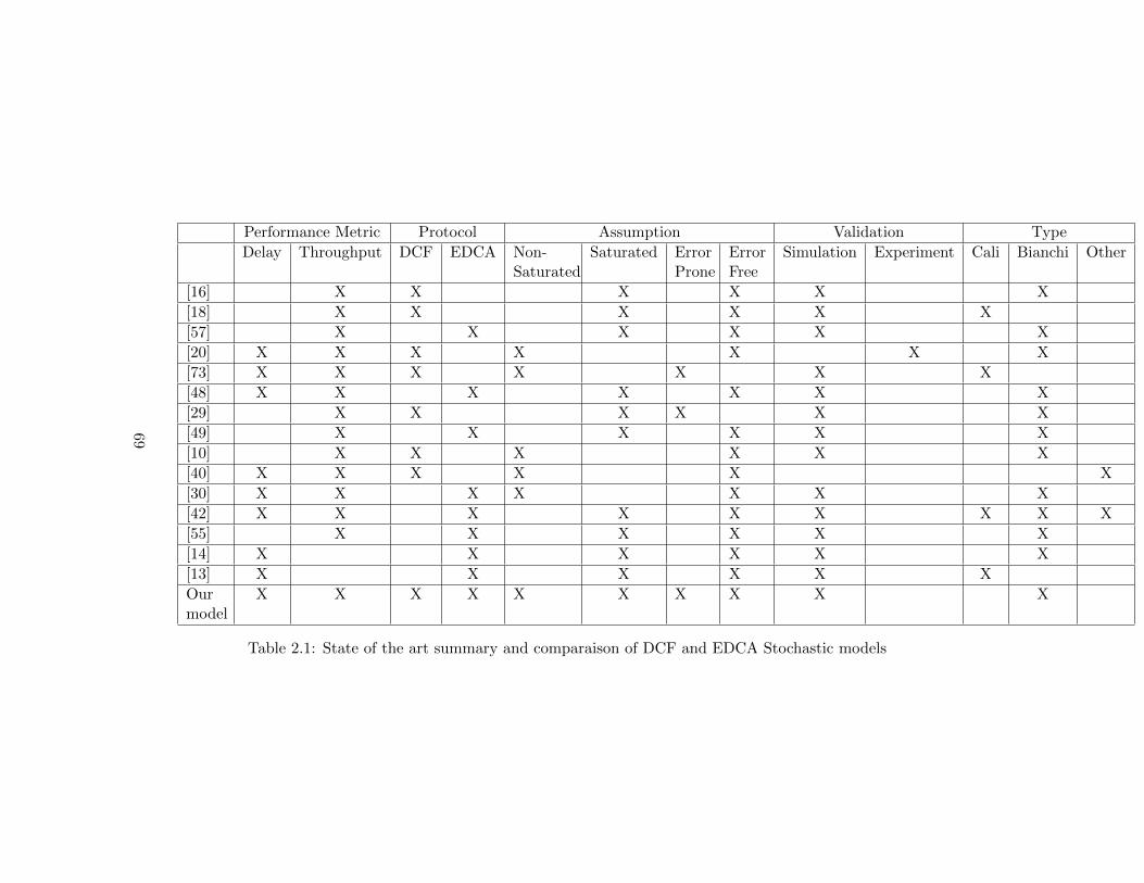
Performance Metric Protocol Assumption Validation Type

Delay Throughput DCF EDCA Non-Saturated

Saturated ErrorProne

ErrorFree

Simulation Experiment Cali Bianchi Other

[16] X X X X X X

[18] X X X X X X

[57] X X X X X X

[20] X X X X X X X

[73] X X X X X X X

[48] X X X X X X X

[29] X X X X X X

[49] X X X X X X

[10] X X X X X X

[40] X X X X X X

[30] X X X X X X X

[42] X X X X X X X X X

[55] X X X X X X

[14] X X X X X X

[13] X X X X X X

Ourmodel

X X X X X X X X X X

Table 2.1: State of the art summary and comparaison of DCF and EDCA Stochastic models

69

Chapter 3

Frequency Allocation toFemtocell

3.1 Introduction

Literally the term femtocell in the context of cellular networks refers tothe size of a cell covered by a Home Base Station (HBS). It is the logicalextension of the already existing sizes which are macrocell, microcell andpicocell. Whereas a picocell is mainly intended for densely populated areassuch as airports, malls, etc., a femtocell is a Personal Base Station that canbe deployed in each house. It has been more than ten years since operatorsstarted to reduce the size of the cell covered by a Base Station (BS) tosupport an increasing number of subscribers and to support large numberof concentrated indoor users. The need to provide high quality coverageindoors became more critical when data oriented services were introduced,because such services require higher throughput in order to be consideredattractive. Even after the appearance of the CDMA technology which led tothe Third Generation (3G) technology, the problem of throughput remains.In addition, as people use their cell phones more and more, the indooruse of mobile phones increases. Since 2002, mobile subscribers worldwidehave outnumbered fixed-line subscribers [43]. The indoor environment is sochallenging that users were rapidly dissatisfied and looked for an alternative.Some alternatives recently considered are the use of relay [58] or multi-hopnetworks [51].

Recent years have brought an exponential increase in the use of wirelessaccess to the internet at home. As the deployment of wireless routers in-creased, and with the introduction of Voice Over IP (VoIP) software, which

70

allows for free phone calls, people wanted to mix these two opportunities.This gave birth to the Dual-Mode handset, which consists of a mobile devicesupporting both cellular technology standards such as GSM, and wireless lo-cal area network standards such as the IEEE 802.11 standard promoted bythe WiFi alliance. This ”smart” solution began to be, and still is, a realthreat for cellular operators as some users no longer use outdoor cellularnetworks deployed by operators to make their indoor phone calls but in-stead use their cheaper access to the internet. That is why the concept offemtocell started gaining prominence about two years ago. In fact the con-cept of femtocell (also called HBS) is not really new. It has already beenproposed in the mid-90 by Silventoinen et al. with the GSM-based HBS [61].It was thought of as a device that a GSM subscriber could buy and connectto his fixed telephone (PSTN) line. This concept has even been standard-ized within European Telecommunications Standards Institute (ETSI) [2]few years later and referred as GSM Cordless Telephony System (CTS)).However this innovation did not attract much attention of the manufactur-ers then, but can now be considered as the seminal work of what we callfemtocell. Actually this is seriously considered by operators who are strug-gling to keep their subscribers loyal. It’s also worth mention that about 10years ago, before HBS was proposed, a similar concept was also considered.It consisted in one handset which would be connected to the regular cellularnetwork when outdoor but as soon as the user entered the home it wouldconnect to the Wireless Private Branch eXchange (PABX) which is the pre-decessor to actual cordless telephone technology such as Digital EnhancedCordless Telecommunications (DECT).

3.2 Description

”To be considered as a candidate” to own a femtocell, a user must have abroadband connection to the internet. The user then must buy a box similarin appearance to a regular WiFi router and plug it into the home network.It is important that a femtocell remains a simple Plug-and-Play device, asa complex installation process is likely to prevent clients from adopting it.When the user enters their home, the femtocell will detect the mobile hand-set and vice versa, and a connection will be established. Then all phonecalls initiated by the mobile handset from indoors will be supported by thefemtocell. The underlying technology to be used can be theoretically oneof the three last generations: 2G (e.g. GSM), 3G (e.g. UMTS) or 4G (e.g.Long Term Evolution (LTE)). The technical challenges are clearly different

71

whether we choose 2G which is based on Time Division Multiple Access(TDMA), 3G based on CDMA or 4G based on Orthogonal Frequency Di-vision Multiple Access (OFDMA). As 3G systems are currently deployedworldwide, we will focus here on this specific technology. In the context of3G the HBS is called Home Node B where Node B stands for the classicmacrocell BS. We will however refer to it further simply as femtocell. 3Gtechnology is based on CDMA which means that all the users can transmitat the same time over the whole bandwidth. To distinguish between sig-nals from different users, different spreading codes are used for each user.CDMA based systems have full frequency reuse which means that the samespectrum is reused in all adjacent cells. To overcome the problem of Co-Channel Interference, power control and scrambling codes which distinguishbetween downlink signals from two different base stations are used. When aMobile Station (MS) moves closer to the edge of its current cell, the processof handover is triggered. The introduction of an additional tier in this al-ready heavy loaded and complex cellular architecture system exhibits severalchallenges.

3.2.1 Access Control

Users can be classified in two categories, depending on the connectivity rightsthat they are given to the Femtocell Access Point (FAP) [74]:

• A subscriber of a femtocell is a user registered in it

• A non-subscriber is a user not registered in the femtocell

According to 3GPP, three access methods to the femtocells, have beenproposed: closed access, open access and hybrid access. The closed accessmode is also called Closed Subscriber Group (CSG). In CSG only subscriberscan connect to their femtocell whereas open access femtocells are accessibleby everyone. In hybrid access, subscribers have a preferential access to theirfemtocell, and non-subscribers have the right to connect with limited accessto the femtocell resources [53]. If we consider 3G technologies, the problemof Co-Channel Interference (CCI) can be unbearable and for this reason openaccess should be mandatory, even though manufacturers actually, use someadvanced techniques to overcome CCI. In fact in 3G technologies, the CDMAtechnique allows full frequency reuse but on the other hand strong powercontrol has to be carried out and it is not always possible with femtocell.With the 4G technologies based on OFDMA, CCI can be mitigated throughpartial frequency reuse as we will show further in section 5.1, and thus open

72

access is not necessary. For this reason we consider here that access to afemtocell should be granted only to the user who owns it in other wordsCSG method.

3.3 Challenges

One of the main challenges with femtocell lies in radio resource manage-ment. We need to remind ourselves that this issue is less critical in the caseof WLAN, where access points do not have to co-exist with an overlayingmacrocell. Moreover the access mechanism of the WiFi technology relies oncarrier sense and collision avoidance mechanism, which avoids interference(for further details see Chapter 2). Nevertheless, femtocells have to take intoconsideration the neighboring femtocells and also the overlaying macrocells.We list four interference scenarios that could occur when a FAP serves aFUE (see also [7]). In fact there are also other scenarios such as femtocellto Macrocell Uplink attack etc., but they are quite similar to the ones wepresent in the following paragraphs.

3.3.1 Femtocell to Macrocell Downlink Interference

Assume a MUE receiving data from its far MAP, for example, we considerthe MUE located at the edge of the cell covered by its MAP. Consequentlythe received signal at the MUE is very low due to the distance between MAPand MUE. Meanwhile a FUE very close to the MUE is receiving data from itsFAP, e.g. when a pedestrian is walking along the edge of the street near theFUE home, or even a user who does not belong to the FAP subscriber group.As the FAP is likely to be close to the FUE, the downlink transmissionbetween the FAP and the FUE will strongly disturb the ongoing downlinktransmission in the macrocell. Under certain conditions it could even leadto a dropped call for the MUE.

3.3.2 Macrocell to Femtocell Uplink Interference

In this attack we assume that the MUE is transmitting to its far MAP.It requires a high transmission power so that the MAP could be able toreceive the signal over the reception power threshold. At the same time, aFUE is transmitting to its FAP. Given their location are so close, the FUEcan transmit at a low power. This feature is important because it can savethe power battery of the FUE. Thus, the consequence is that the uplinktransmission in the femtocell will be strongly interfered by the MUE.

73

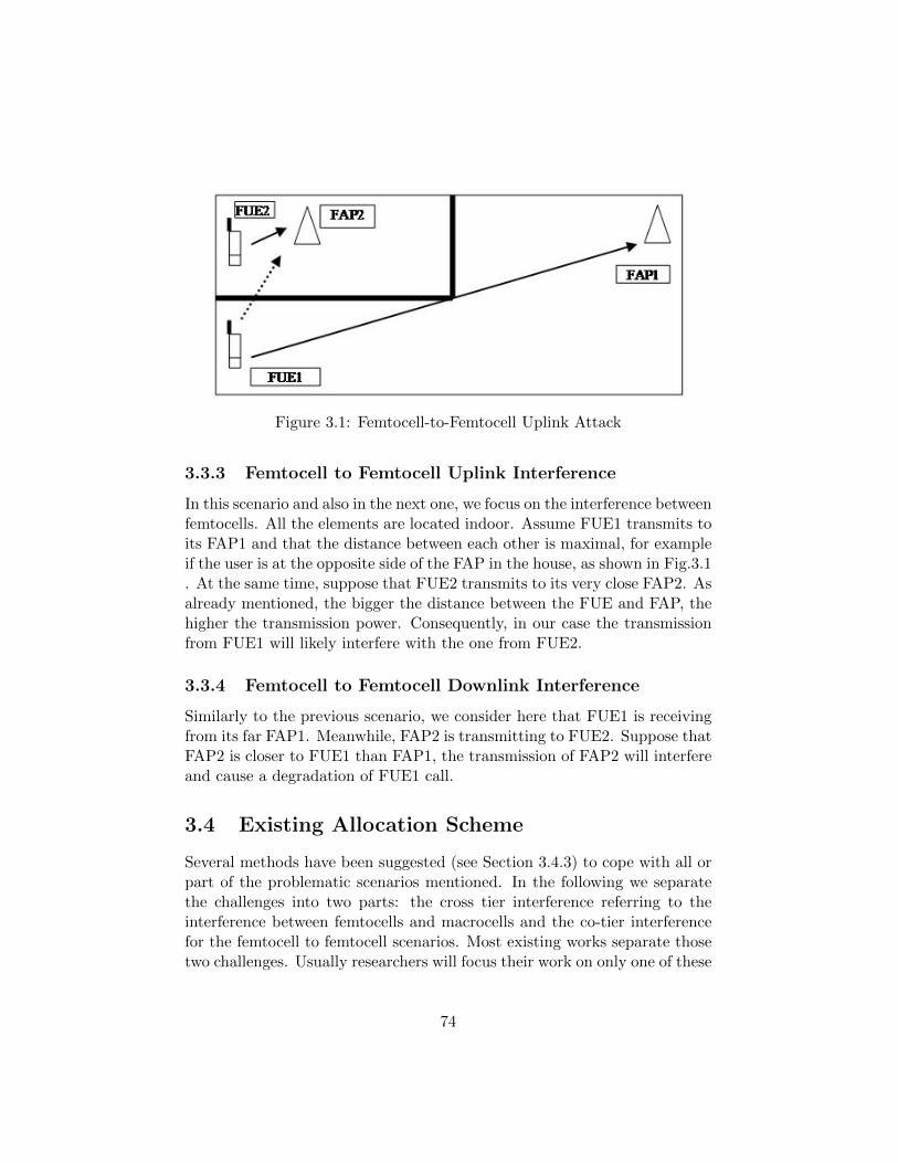
Figure 3.1: Femtocell-to-Femtocell Uplink Attack

3.3.3 Femtocell to Femtocell Uplink Interference

In this scenario and also in the next one, we focus on the interference betweenfemtocells. All the elements are located indoor. Assume FUE1 transmits toits FAP1 and that the distance between each other is maximal, for exampleif the user is at the opposite side of the FAP in the house, as shown in Fig.3.1. At the same time, suppose that FUE2 transmits to its very close FAP2. Asalready mentioned, the bigger the distance between the FUE and FAP, thehigher the transmission power. Consequently, in our case the transmissionfrom FUE1 will likely interfere with the one from FUE2.

3.3.4 Femtocell to Femtocell Downlink Interference

Similarly to the previous scenario, we consider here that FUE1 is receivingfrom its far FAP1. Meanwhile, FAP2 is transmitting to FUE2. Suppose thatFAP2 is closer to FUE1 than FAP1, the transmission of FAP2 will interfereand cause a degradation of FUE1 call.

3.4 Existing Allocation Scheme

Several methods have been suggested (see Section 3.4.3) to cope with all orpart of the problematic scenarios mentioned. In the following we separatethe challenges into two parts: the cross tier interference referring to theinterference between femtocells and macrocells and the co-tier interferencefor the femtocell to femtocell scenarios. Most existing works separate thosetwo challenges. Usually researchers will focus their work on only one of these

74

challenges at a time. Thus we will present the state of the art in two separateparts for each of them. In section 3.4.3 we present the solutions proposedto deal with the problems of frequency allocation to hierarchical multilayercells. Then in section 3.4.4 we present the multiple algorithms and schemesto allocate radio resources to different stations belonging to the same tier.However because some solutions were presented specifically at the macrocellor even at the femtocell level we further subdivide this part into two groupsof solutions : the macrocell layer and the femtocell layer (each one will bepresented separately). Finally we summarize in Table 3.1 the characteristicsof most of the solutions presented. This would allow someone faced with aspecific challenge to quickly find a solution fitting to a similar problems.

3.4.1 Introduction

It is interesting to note that as we mentioned in the introduction above, theconcept of femtocell is not so new and was already considered at the end ofthe 80’s. However even though some papers already considered the issue offrequency assignment for this second tier system, recent papers on femtocelldo not mention them generally. A possible reason is that the term usedin those days was different from the one we use today, so some importantresults can easily be overlooked. Here we propose to list the different termsfound in the early literature which dealt with the concept of femtocell butwhich did not refer to it with this latter name:

• CTS where the access point is called CTS Fixed Part (CTS-FP)

• indoor Base Station (BS)

• indoor cellular radio PBX(private Branch Exchange)

• Home Base Stations (HBS)

• digital cordless telephone PBX [71]

• indoor cellular system/radio [46]

• indoor microcel for cordless telephone PBX [36]

In fact, another second tier was also considered some time before at theend of the 80’s: the Microcell. The concept of hierarchical networks or multi-tier (also called multilayer) cellular systems rapidly appeared to be a logicalextension of the cellular system. Hot spot are covered by microcells (layer 1)while macrocells provide a continuous coverage of the service area (layer 2).

75

In very dense areas, a continuous coverage with both microcells and macro-cells may be achieved [50]. However the intensive deployment of microcellBSs is generally more expensive than conventional macrocells deploymentbecause of the potentially high number of sites. Hierarchical architecturehas to be carefully optimized so that both layers can act complementarily[23]. Thus some papers already dealt, with the issue of the efficient useof the spectrum between Macrocell and Microcells in these years. We thusobviously learned from this method to apply them naturally to the newextension layer: the Femtocell.

3.4.2 Experimental Results in the Literature

In [69], a series of experiments were reported. Even though effective airlinkdata rate was measured, the main data captured was Signal to Interfer-ence and Noise Ratio (SINR) to concentrate on coverage quality rather thanapplication layer throughput so as to be independent of the Internet andbackhaul. The conclusion of the study is that femtocells outperform macro-cells in terms of broadband airlink data rates by almost five to one. Theauthors also defend that the main benefits of femtocells over macrocells isfor data services since voice services are not really ”hungry” in bandwidthand therefore do not provide additional value compared to the macrocelloffered service. However the main drawback of this study is that femtocellswere deployed in a dedicated carrier thus avoiding interference from macro-cells which is actually one of the most challenging issues for 3G femtocells.Besides the interference between femtocells is obviously not taken into ac-count as the experiment rely on only dozens of femtocells spread over thewhole world. Nevertheless the measurements constitute a good database forengineers who are developing simulators and can also be considered for sur-veys of femtocell in 4G where dedicated spectrum is possible and seriouslyconsidered.

3.4.3 Cross-Tier Allocation Scheme

The first to consider frequency reuse of the overlaying macrocell by a secondlayer system was Kinoshita et al. in [46]. They introduced the concept of”frequency Double Reuse” (DR) technique, which allows urban frequencychannels to be also used in indoor cordless telephone systems. They furtherextend this idea to the coexistence between macrocell and microcell systemsin [45] and [47] where the frequency channel used in the nearby cell is reusedin a microcell inside the same cluster of macrocells and considered by the

76

authors as a high density space division multiple access (SDMA). This latterwork has been extended by [35] to consider Dynamic Channel Assignment(DCA). The authors argue that it is hard to plan channel reuse in advancebetween the macrocells and microcells, since the wave propagation becomeshighly irregular in the microcells. Therefore the Fixed Channel Assignment(FCA) proposed by Kinoshita et al.. seems to be impossible in the microcellssystems overlaid with macrocells. However [35] still requires power controland an increase in the implementation cost. In [68] a tradeoff between FCAand DCA is proposed. A classic 7-cluster reuse is used but the sectors arearranged in an original manner. It is proposed to rotate the sectors in eachcell in a way that would avoid interference from co-channel adjacent sectors.

In [62], Silventoinen addressed the problem of allocating frequency toGSM-based femtocells (referred therein as Home Base Station). A TotalFrequency Hopping (TFH) is used where transmissions of differents HBSstake place in differents carrier frequencies and the hopping is spread overall the available carriers the operator has in a pseudo-random way. Thehopping sequences for individual HBSs are independent of each other. TheTFH scheme eliminates the need for frequency planning since all frequenciesare used in a pseudo-random manner and the additional interference to theoverlaying system is evenly distributed over the whole spectrum in use. Theconclusion for the downlink (the only direction simulated there) is that ifHBS power is about 40 dB less than in macro networks, negative effect ofthe macro on the second layer HBS is negligible. Further investigation ontransmission power for HBS, and effects on macro layer following the densityof HBSs can be found in [27].

For the cross-tier interference, two main approaches are possible : Spec-trum splitting or spectrum sharing. In the first approach macro and femto-cells are given orthogonal frequency bands, also referred to as ”orthogonalsharing” [50],[31]. This approach seems to be the simplest one, as no crosstier interference is expected. Thus both macro and femtocell tiers can beconsidered as totally separate networks. However a drawback is, that itis not efficient, because splitting the already allocated spectrum into twosmaller ones would imply lower throughput to macrocell users which is notdesirable. Moreover even in the rare case of an operator with a large spec-trum for which this approach is a simple and straight-forward solution, anoptimum division of the spectrum between the layers still has to be derived[33], which is not an obvious issue [34]. In the spectrum sharing approachthe same spectrum is used by the macro and femtocell infrastructure, whichobviously leads to the critical problem of co-channel interference. A thirdpossible approach is that the different layers share several radio frequencies

77

but not at the same time [31]. Such a dynamic sharing may be provided bymeans of dynamic channel allocation.

In [24], the authors evaluate four approaches to sharing the spectrumbetween microcells and macrocells . The first two feature spread-spectrumsharing, i.e., they use TDMA among microcell users and CDMA amongmacrocell users (System I), or vice versa (System II). The other two ap-proaches feature orthogonal sharing, i.e., they use TDMA in both tiers,with time slots (System III) or frequency channels (System IV) partitionedso there is no overlap between tiers. It is concluded that spread spectrumbetween layers is possible but will provide poor capacity because of the largeamounts of cross-tier interference. The best approach is the simplest one:use different frequencies for different layers (System IV).

In [28] they study the ability of hierarchical cellular structures with inter-layer reuse to increase the capacity of a GSM radio network by applyingTotal Frequency Hopping (TFH) similarly to [61] and Adaptive FrequencyAllocation (AFA) as a strategy to reuse the macro- and microcell resourceswithout frequency planning in indoor picocells. In the macro- and microcelllayer different frequencies are used to avoid the coordination effort betweenthe layers. At the picocell level several scheme are proposed: reuse partor all of the frequencies of either only Macro or Microcell spectrum whereless interfered channels are selected. Partial loading is assumed in eachof the layers.One of the interesting conclusions of this study is that it ismore efficient to exclude the strongest interferers than to achieve a higherinterference averaging gain by using as much frequencies as possible for TFH.Unlike [28] where Macrocell and microcell use different frequency bands, in[11] a frequency reuse scheme where microcell reuse the macrocell frequencyis proposed. However there are some limitations: microcells can reuse onlychannels used neither by the overlaid macrocell nor by the adjacent cellwhich would lead to adjacent channel interference. Moreover it has beenshown there that microcell users have to transmit in the Uplink at a powerlevel at least 10 dB below macrocell users, because of the interference inducedby microcell users on the Macrocell. However Microcell BSs have to transmitwith the same power as Macrocell BS, to be ”heard”by microcell users in thedownlink. This latter condition is possible because the macrocell downlinkis almost unaffected, due to the isolation of the micro BSs. It is important tonotice that interference between microcells (Micro to Micro) is not studied.

In [39], a frequency assignment for femtocells is proposed. The coverageof the macrocell is split into 2 regions: inner and outer regions. If a femtocellis located in the outer region, it can reuse the channel of the overlayingmacrocell. However if the femtocell is in the inner region, it must use a

78

different channel than the overlaying macrocell. To compute where the limitmust be between inner and outer region, the ILCA (Interference-limitedcoverage area) of a femtocell is defined. It is the area within a contourwhere the received power levels from the FAP and MAP are the same. Ifthe ILCA is above a threshold, the femtocell is considered in the inner region.This frequency assignment method applies only to downlink, and it is notmentioned in [39] which frequency is allocated to the femtocells located inthe inner region.

In [44], an uplink femtocell power control is proposed. It reduces thecross tier interference at the macrocell level. The study is in the contextof the OFDMA WiMax system which can be also useful for LTE systems.However the power control proposed is not always realistic. In some cases,controlling the uplink transmission power of the femtocell to not disturb themacrocell, can lead to too low transmitted power and the FUE could notbe covered by its FAP. Another solution proposed, is to share the resourcein a TDMA fashion manner on top of the CDMA [21]. Macrocell and fem-tocell will each transmit independently over one time slot and remain silentover other slots. This is referred to as Time Hopped-CDMA (TH-CDMA).However it is in fact equivalent to splitting the resources in the time domaininstead of splitting them in the frequency domain. As already mentioned forspectrum splitting, the loss of resource efficiency in an environment whereradio resources are so scarce constitutes a major drawback.

3.4.4 Co-tier allocation scheme

In the following paragraphs we present some of the algorithms developedto allocate channels to the users of a single layer. We did not detail thispart because (as we will see further) we did not propose in this thesis anovel scheme of channel allocation between femtocells. We assume thata simple allocation based on best SINR is enough to be able to retrieveinteresting results on our double frequency reuse schemes and therefore toassess potential performance of femtocells. However we find useful to bringhere some references to existing work, especially to illustrate some of thecharacteristics of the femtocell mentioned above in section 3.2 such as AccessControl subsection 3.2.1. Moreover we get inspired from some of these worksfor the frequency allocation scheme we will proposed further in Chap. 5.

79

Macrocell layer

When we deal with frequency planning at the macrocell level we need inparticular to consider the underlying multiple access mechanism. For ex-ample it is well known that in CDMA systems, the Frequency Reuse Factor(FRF) is equal to 1. Transmission to and from different users can be sepa-rated thanks to scrambling and spreading codes [70]. However in OFDMAsystems, if the FRF is also equal to 1, this may lead to CCIs due to the si-multaneous use of the same subchannels by different users in adjacent cells.Thus one of the challenges thoroughly studied in the literature is how toassign and reuse the scarce bandwidth to reduce CCI. Obviously, increasingFRF is not really spectrum efficient.

The use of Frequency Hopping techniques applied to OFDMA referredto as frequency hopping OFDMA (FH-OFDMA) which uses the frequencydiversity by interleaving and spreading the transmitted subcarriers over thewhole bandwidth, and averages the inter-cell interference is considered in[63] and [67]. In [52] splitting each cell into two region is proposed. Thefirst region is the central region close to the BS and the second region is theedge which is itself split into three sector. The channel allocation is done asfollowing : two groups of frequencies are defined: the super group and theregular group. The central region uses frequencies only from the super groupwith FRF=1 whereas the edge uses frequencies from the regular groups splitinto the 3 sectors with FRF =3 . Regular Group reuses frequencies of thecentral region of other cells, but not from its own cell since it would lead tosevere intra-cell interference.

In [37], resource allocation on OFDMA context is considered but onlyat the macrocell level. Centralized and distributed scheme is proposed. Incentralized the allocation is done in 2 steps: at the high level an allocationin the time domain is achieved where a sets of Resource Block (RB) (whichis the unity of resource in LTE) is allocated to each MAP. This is done bya central coordinator which implements an algorithm which minimize theintercell interference. Then in a more fine time domain, each BS allocatea RB to a user based on an algorithm such as proportional fairness. Inthe distributed scheme, allocation is done thanks to power profile defineda-priori. Thus each cell know by advance to which level of interference itwill be exposed. These propositions even though interesting cannot be usedfor femtocell as it requires a central coordinator. Even for the distributedscheme, profiles have to be already defined which is not really possible withfemtocell which is plug and play without operator’s planning before.Besidesalgorithm to define the power profile is not defined in this paper but pre-

80

sented as an open issue.

Femtocell layer

A self-organized resource allocation algorithm for femtocell is presented in[54]. A sub-channel is allocated to a Femtocell based on either local broad-cast messages from neighbouring FAP referred to as broadcast approach orfrom FUE measurement periodical report. In the broadcast approach, a”badness” indicator for each subchannel is computed. This indicator reflectsthe probability of usage and the intensity of interference for the sub-channel.In the second approach, each FUE sends a measurement report to its serv-ing FAP which indicates the RSS suffered by the user in each sub-channel.Then the FAP gathers the information received from all of its FUEs andbuilds an interference matrix. A new subchannel is chosen following anoptimization procedure whose target is to minimize the sum of the overallinterference suffered by the users of the femtocell .This paper does not dealwith the spectrum allocated originally to the femtocell but considers it asgiven. Besides prediction of interference which is needed for computationof the ”badness” indicator is based on too simple propagation model whichis mainly the free space loss model with added loss for wall penetration.However indoor wireless channels is well known for suffering from fading sowe lack a more reliable propagation model.

Effects of open access versus CSG to femtocell to outside users have beenanalyzed in [66]. It shows that when CSG is used the outage probability fornon-subscriber users is high whereas if even one sub-channel is reserved forthem, the outage probability not only decreases but resources reserved canbe sufficient if non-subscribers request voice services. An interesting obser-vation is that if the quantity of subchannels reserved is low, then even if thenumber of femtocells deployed increases the outage probability increases dueto cross tier interference on non-subscribers not yet associated with the fem-tocell. It proposes that providers or femtocell owners define minimum num-bers of subchannels available to non-subscribers in a dynamic manner. It isworth mentioning that the coverage is predicted using the Finite-DifferenceTime-Domain (FDTD) method based on ray tracing theory which can beconsidered as very accurate. However the number of MUE users does notincrease to up than 5 meanwhile which is not really representative of anurban or even sub-urban area.

81

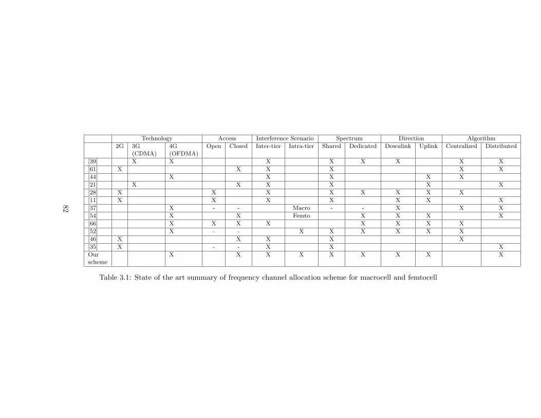
Technology Access Interference Scenario Spectrum Direction Algorithm

2G 3G(CDMA)

4G(OFDMA)

Open Closed Inter-tier Intra-tier Shared Dedicated Downlink Uplink Centralized Distributed

[39] X X X X X X X X

[61] X X X X X X

[44] X X X X X

[21] X X X X X X

[28] X X X X X X X X

[11] X X X X X X X

[37] X - - Macro - - X X X

[54] X X Femto X X X X

[66] X X X X X X X X

[52] X - - X X X X X X

[46] X X X X X

[35] X - - X X X

Ourscheme

X X X X X X X X X

Table 3.1: State of the art summary of frequency channel allocation scheme for macrocell and femtocell

82

Part II

Our Proposition

83

Chapter 4

Stochastic Model of EDCA

4.1 System Model

Our work is an improvement of the IEEE 802.11 and IEEE 802.11e existingmodels, and we chose to follow the methodology presented in [48]. Indeed,our objective is to provide a more realistic and extensive model. Thus, wesuggest the following improvements: we consider a non-ideal channel (i.e.,which introduces errors into the packets, according to a fixed error proba-bility), and we consider that stations may be idle (i.e. the emission bufferof the network card can be empty). Indeed, assuming an ideal channel is arather coarse simplification in the field of wireless transmission. Moreover,the saturated medium which is usually considered to evaluate the capacityof the network only indicates the maximum capacity of the link. Up to ourknowledge, there is no EDCA model that takes into account a non-idealchannel under finite load.

4.1.1 Four Dimensional Markov Chain

The Markov chain represented in Fig. 4.3 models the behavior of an accesscategory (AC) managed by EDCA, for a given station. In order to sim-plify the diagram, we did not represent all the transition probabilities fromone state to another. Our model comprises a great number of indices andvariables, which are summarized in Table 4.1.

The so-called Bianchi model is based on a two dimensional Markov chain.The second dimension b(t), indicates the value of the backoff timer, whichcorresponds to the number of time slots to wait before being able to re-initialize a transmission after a failure. This model fits well to a saturatedmedium because it assumes that at any point in time, STAs have data to

84

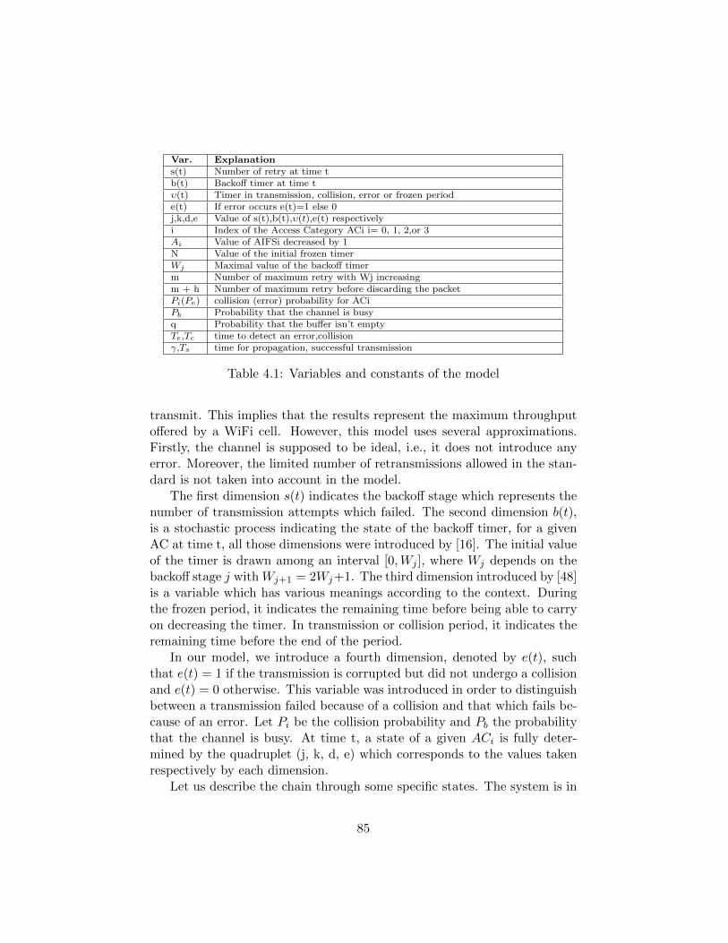
Var. Explanations(t) Number of retry at time tb(t) Backoff timer at time tυ(t) Timer in transmission, collision, error or frozen periode(t) If error occurs e(t)=1 else 0j,k,d,e Value of s(t),b(t),υ(t),e(t) respectivelyi Index of the Access Category ACi i= 0, 1, 2,or 3Ai Value of AIFSi decreased by 1N Value of the initial frozen timerWj Maximal value of the backoff timerm Number of maximum retry with Wj increasingm + h Number of maximum retry before discarding the packetPi(Pe) collision (error) probability for ACiPb Probability that the channel is busyq Probability that the buffer isn’t emptyTe,Tc time to detect an error,collisionγ,Ts time for propagation, successful transmission

Table 4.1: Variables and constants of the model

transmit. This implies that the results represent the maximum throughputoffered by a WiFi cell. However, this model uses several approximations.Firstly, the channel is supposed to be ideal, i.e., it does not introduce anyerror. Moreover, the limited number of retransmissions allowed in the stan-dard is not taken into account in the model.

The first dimension s(t) indicates the backoff stage which represents thenumber of transmission attempts which failed. The second dimension b(t),is a stochastic process indicating the state of the backoff timer, for a givenAC at time t, all those dimensions were introduced by [16]. The initial valueof the timer is drawn among an interval [0,Wj ], where Wj depends on thebackoff stage j with Wj+1 = 2Wj+1. The third dimension introduced by [48]is a variable which has various meanings according to the context. Duringthe frozen period, it indicates the remaining time before being able to carryon decreasing the timer. In transmission or collision period, it indicates theremaining time before the end of the period.

In our model, we introduce a fourth dimension, denoted by e(t), suchthat e(t) = 1 if the transmission is corrupted but did not undergo a collisionand e(t) = 0 otherwise. This variable was introduced in order to distinguishbetween a transmission failed because of a collision and that which fails be-cause of an error. Let Pi be the collision probability and Pb the probabilitythat the channel is busy. At time t, a state of a given ACi is fully deter-mined by the quadruplet (j, k, d, e) which corresponds to the values takenrespectively by each dimension.

Let us describe the chain through some specific states. The system is in

85

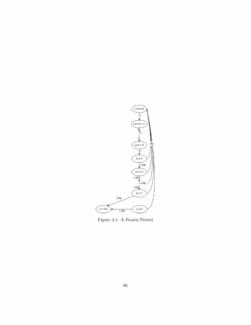
Figure 4.1: A Frozen Period

86

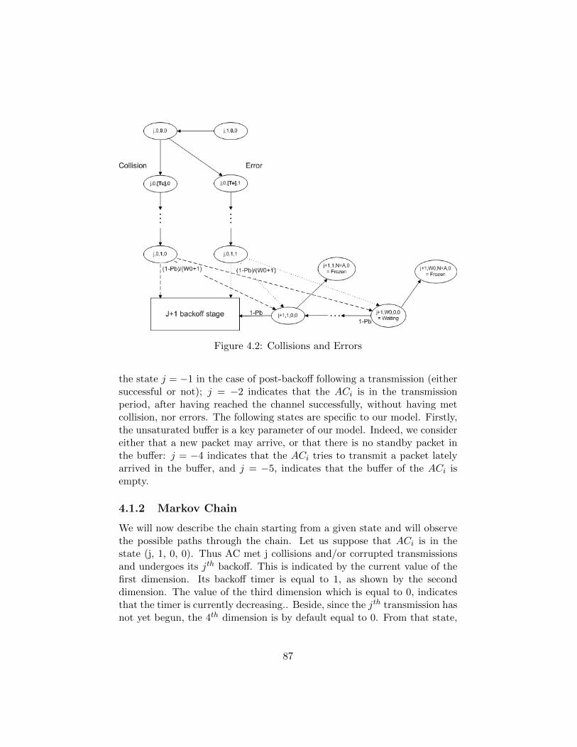
Figure 4.2: Collisions and Errors

the state j = −1 in the case of post-backoff following a transmission (eithersuccessful or not); j = −2 indicates that the ACi is in the transmissionperiod, after having reached the channel successfully, without having metcollision, nor errors. The following states are specific to our model. Firstly,the unsaturated buffer is a key parameter of our model. Indeed, we considereither that a new packet may arrive, or that there is no standby packet inthe buffer: j = −4 indicates that the ACi tries to transmit a packet latelyarrived in the buffer, and j = −5, indicates that the buffer of the ACi isempty.

4.1.2 Markov Chain

We will now describe the chain starting from a given state and will observethe possible paths through the chain. Let us suppose that ACi is in thestate (j, 1, 0, 0). Thus AC met j collisions and/or corrupted transmissionsand undergoes its jth backoff. This is indicated by the current value of thefirst dimension. Its backoff timer is equal to 1, as shown by the seconddimension. The value of the third dimension which is equal to 0, indicatesthat the timer is currently decreasing.. Beside, since the jth transmission hasnot yet begun, the 4th dimension is by default equal to 0. From that state,

87

two possibilities arise . If ACi observes a busy channel, the backoff timer isfrozen (see Fig.4.1), which involves the beginning of the frozen period, andbrings ACi to state (j, 1, N+Ai, 0). Otherwise, the systems goes to (j, 0,0, 0). This cycle is repeated until ACi can reactivate its timer and accessesthe channel. At this point, if no higher priority ACi′ (within the same STAor another STA) tries to transmit at the same time, ACi will access thechannel and transmit its packet. However, if a collision or an error occurs,a certain time respectively Tc or Te will be required before ACi becomesaware of this collision or respectively of this error, and passes to state j+1for a new attempt.

4.1.3 Characteristic of Our Model: the Unsaturated Mode

After a successful transmission, if the buffer already has a new packet instandby (with a probability q), then ACi enters state j = -1. If the bufferis empty (with a probability 1-q), ACi enters a waiting state noted (-5, 0,0, 0). In each Time Slot, ACi, checks its buffer, if it still does not containa new packet to be transmitted it remains in the same state (-5, 0, 0, 0).On the other hand, if a new packet arrives in the queue, the ACi moves tostate (-4, 0, Ai, 0), which allows it to access the channel directly after havingchecked that it remained free for a certain time (AIFSi).

This is a major difference with the saturated models that assume a STAalways has a packet to transmit, in other words, that its buffer is neverempty. Therefore, when a new packet arrives, it has to wait and initiate abackoff, instead of being sent directly after an AIFS. In our model, we intro-duced (-4,0,d,0), d=0..Ai to correct this approximation. The introductionof this state, namely (-5,0,0,0), is fundamental, since a STA does not alwayshave data to transmit. Thus, we can consider the possibility of having anempty buffer. In addition, compared to existing models, we add significantvalue by allowing to represent different load scenarios using parameter q.

4.1.4 Transition probabilities

We will now describe the transition probabilities from one state to another.

1. For states (-2, 0, d, 0), d = 1,2,..., [Ts],

• P{(−2, 0, d− 1, 0)/(−2, 0, d, 0)} = 1

2 ≤ d ≤ [Ts]

88

Account for the fact that, during the transmission, time is decre-mented.

• P{(−1, 0, Ai, 0)/(−2, 0, 1, 0)} = q

After a successful transmission, when a new packet is already waitingin the buffer

• P{(−5, 0, 0, 0)/(−2, 0, 1, 0)} = 1− q

When the buffer is empty

2. For states (j, 0, 0, 0), j = 0, 1,..., m+h,

• Successful transmission if no collision nor error occurs.

P{(−2, 0, [Ts], 0)/(j, 0, 0, 0)} = (1− Pi)(1− Pe)0 ≤ j ≤ m+ h

• If a collision occurs then ACi enters the collision period

P{(j, 0, [Tc], 0)/(j, 0, 0, 0)} = Pi; 0 ≤ j ≤ m+ h

• If no collision occurs but there is an error

P{(j, 0, [Te], 1)/(j, 0, 0, 0)} = (1− Pi)× Pe; 0 ≤ j ≤ m+ h

3. For state ( m+h, 0, 0, 0),

• If no collision and no error occurs, then the transmission succeed

P{(−2, 0, [Ts], 0)/(m+ h, 0, 0, 0)} = (1− Pi)(1− Pe)

• If a collision or an error occurs after the collision or error period,the packet is discarded because m+h retries have been exhausted.

89

Then the ACi checks his buffer. If a new packet is already waiting:• After an error:

P{(−1, 0, Ai, 0)/(m+ h, 0, 1, 1)} = (1− Pi)Pe × q

• After a collision:

P{(−1, 0, Ai, 0)/(m+ h, 0, 1, 0)} = Pi × q

Let:

Pi + (1− Pi)Pe = Pfi (4.1)

If the buffer is empty:

• After an error:

P{(−5, 0, 0, 0)/(m + h, 0, 1, 1)} = (1 − Pi)Pe × (1 − q)

• After a collision:

P{(−5, 0, 0, 0)/(m+ h, 0, 1, 0)} = Pi × (1− q)

4. For states (j, 0, d, 0), j= 0, 1 ... m+h and d ≥ 1, when a collisionoccurs, time is decremented by 1 for each time slot elapsed, until theACi exits the collision period:

P{(j, 0, d− 1, 0)/(j, 0, d, 0)} = 1

0 ≤ j ≤ m+ h; 2 ≤ d ≤ [Tc]

When the collision period finishes, the ACi doubles the size of theContention Window (CW), except when CW hads already reachedthe maximum value CWmax, and chooses a random number from theuniformly distributed set [0, Wj+1] and then enters the next backoffstage

P{(j + 1, k, 0, 0)/(j, 0, 1, 0)} =1

(Wj+1 + 1)

0 ≤ k ≤Wj+1; 0 ≤ j ≤ m+ h

90

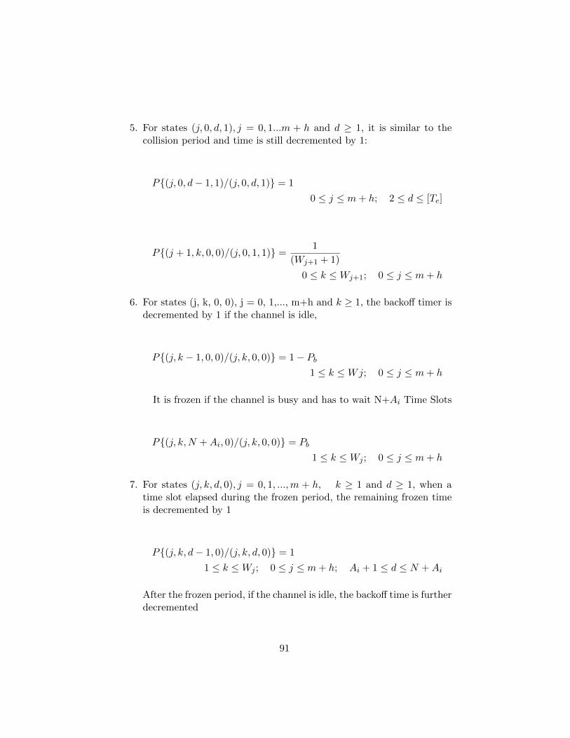
5. For states (j, 0, d, 1), j = 0, 1...m + h and d ≥ 1, it is similar to thecollision period and time is still decremented by 1:

P{(j, 0, d− 1, 1)/(j, 0, d, 1)} = 1

0 ≤ j ≤ m+ h; 2 ≤ d ≤ [Te]

P{(j + 1, k, 0, 0)/(j, 0, 1, 1)} =1

(Wj+1 + 1)

0 ≤ k ≤Wj+1; 0 ≤ j ≤ m+ h

6. For states (j, k, 0, 0), j = 0, 1,..., m+h and k ≥ 1, the backoff timer isdecremented by 1 if the channel is idle,

P{(j, k − 1, 0, 0)/(j, k, 0, 0)} = 1− Pb1 ≤ k ≤Wj; 0 ≤ j ≤ m+ h

It is frozen if the channel is busy and has to wait N+Ai Time Slots

P{(j, k,N +Ai, 0)/(j, k, 0, 0)} = Pb

1 ≤ k ≤Wj ; 0 ≤ j ≤ m+ h

7. For states (j, k, d, 0), j = 0, 1, ...,m + h, k ≥ 1 and d ≥ 1, when atime slot elapsed during the frozen period, the remaining frozen timeis decremented by 1

P{(j, k, d− 1, 0)/(j, k, d, 0)} = 1

1 ≤ k ≤Wj ; 0 ≤ j ≤ m+ h; Ai + 1 ≤ d ≤ N +Ai

After the frozen period, if the channel is idle, the backoff time is furtherdecremented

91

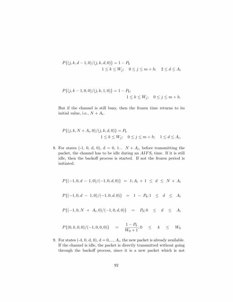
P{(j, k, d− 1, 0)/(j, k, d, 0)} = 1− Pb1 ≤ k ≤Wj ; 0 ≤ j ≤ m+ h; 2 ≤ d ≤ Ai

P{(j, k − 1, 0, 0)/(j, k, 1, 0)} = 1− Pb;1 ≤ k ≤Wj ; 0 ≤ j ≤ m+ h.

But if the channel is still busy, then the frozen time returns to itsinitial value, i.e., N +Ai.

P{(j, k,N +Ai, 0)/(j, k, d, 0)} = Pb

1 ≤ k ≤Wj ; 0 ≤ j ≤ m+ h; 1 ≤ d ≤ Ai,

8. For states (-1, 0, d, 0), d = 0, 1... N + Ai, before transmitting thepacket, the channel has to be idle during an AIFSi time. If it is stillidle, then the backoff process is started. If not the frozen period isinitiated.

P{(−1, 0, d − 1, 0)/(−1, 0, d, 0)} = 1;Ai + 1 ≤ d ≤ N + Ai

P{(−1, 0, d − 1, 0)/(−1, 0, d, 0)} = 1 − Pb; 1 ≤ d ≤ Ai

P{(−1, 0, N + Ai, 0)/(−1, 0, d, 0)} = Pb; 0 ≤ d ≤ Ai

P{(0, k, 0, 0)/(−1, 0, 0, 0)} =1− PbW0 + 1

; 0 ≤ k ≤ W0

9. For states (-4, 0, d, 0), d = 0,..., Ai, the new packet is already available.If the channel is idle, the packet is directly transmitted without goingthrough the backoff process, since it is a new packet which is not

92

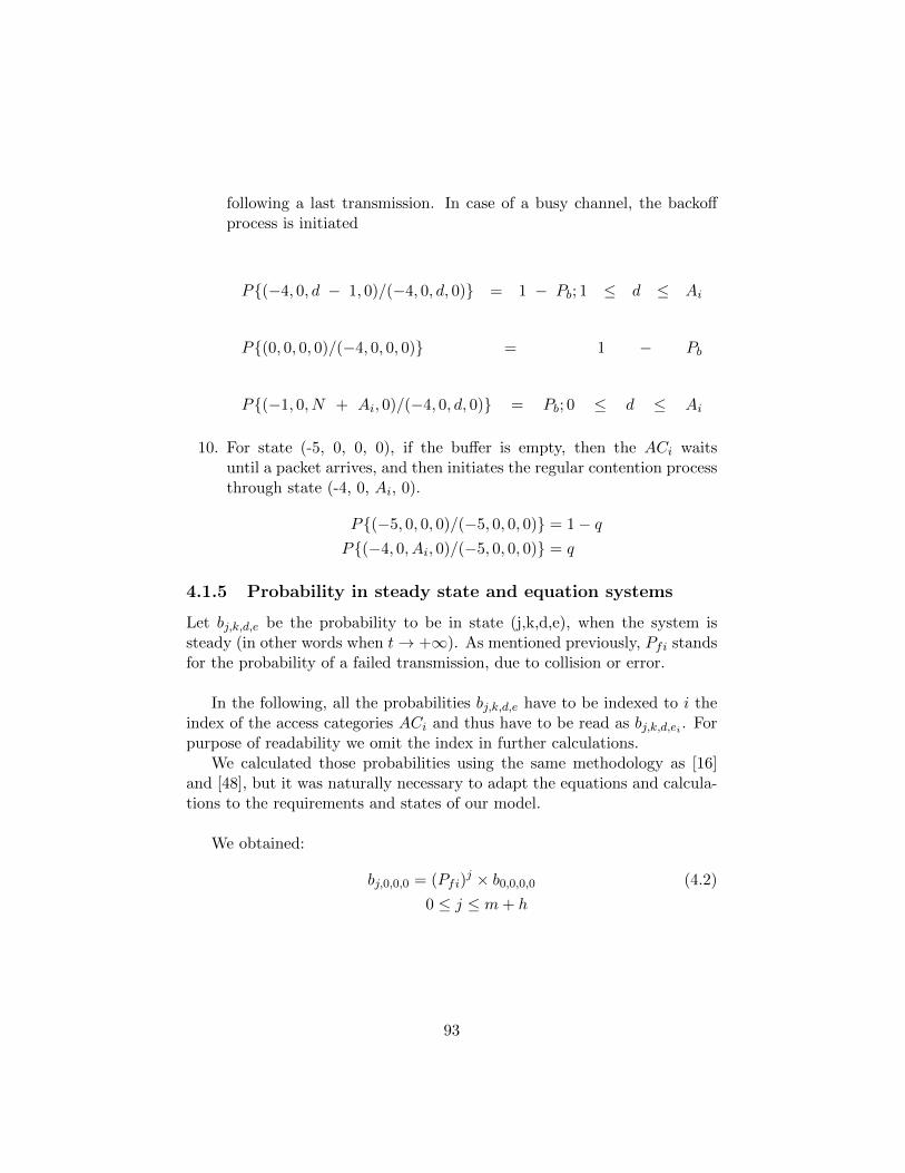
following a last transmission. In case of a busy channel, the backoffprocess is initiated

P{(−4, 0, d − 1, 0)/(−4, 0, d, 0)} = 1 − Pb; 1 ≤ d ≤ Ai

P{(0, 0, 0, 0)/(−4, 0, 0, 0)} = 1 − Pb

P{(−1, 0, N + Ai, 0)/(−4, 0, d, 0)} = Pb; 0 ≤ d ≤ Ai

10. For state (-5, 0, 0, 0), if the buffer is empty, then the ACi waitsuntil a packet arrives, and then initiates the regular contention processthrough state (-4, 0, Ai, 0).

P{(−5, 0, 0, 0)/(−5, 0, 0, 0)} = 1− qP{(−4, 0, Ai, 0)/(−5, 0, 0, 0)} = q

4.1.5 Probability in steady state and equation systems

Let bj,k,d,e be the probability to be in state (j,k,d,e), when the system issteady (in other words when t→ +∞). As mentioned previously, Pfi standsfor the probability of a failed transmission, due to collision or error.

In the following, all the probabilities bj,k,d,e have to be indexed to i theindex of the access categories ACi and thus have to be read as bj,k,d,ei . Forpurpose of readability we omit the index in further calculations.

We calculated those probabilities using the same methodology as [16]and [48], but it was naturally necessary to adapt the equations and calcula-tions to the requirements and states of our model.

We obtained:

bj,0,0,0 = (Pfi)j × b0,0,0,0 (4.2)

0 ≤ j ≤ m+ h

93

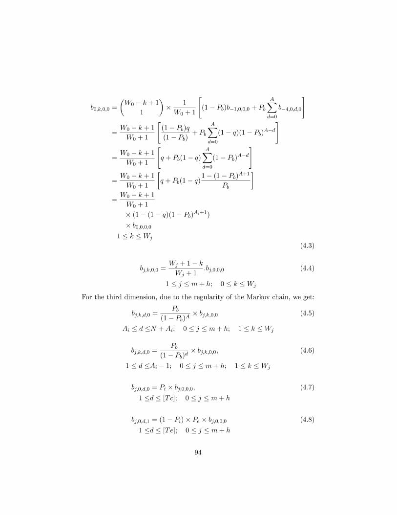
b0,k,0,0 =

(W0 − k + 1

1

)× 1

W0 + 1

[(1− Pb)b−1,0,0,0 + Pb

A∑d=0

b−4,0,d,0

]

=W0 − k + 1

W0 + 1

[(1− Pb)q(1− Pb)

+ Pb

A∑d=0

(1− q)(1− Pb)A−d]

=W0 − k + 1

W0 + 1

[q + Pb(1− q)

A∑d=0

(1− Pb)A−d]

=W0 − k + 1

W0 + 1

[q + Pb(1− q)

1− (1− Pb)A+1

Pb

]=W0 − k + 1

W0 + 1

× (1− (1− q)(1− Pb)Ai+1)

× b0,0,0,01 ≤ k ≤Wj

(4.3)

bj,k,0,0 =Wj + 1− kWj + 1

.bj,0,0,0 (4.4)

1 ≤ j ≤ m+ h; 0 ≤ k ≤Wj

For the third dimension, due to the regularity of the Markov chain, we get:

bj,k,d,0 =Pb

(1− Pb)A× bj,k,0,0 (4.5)

Ai ≤ d ≤N +Ai; 0 ≤ j ≤ m+ h; 1 ≤ k ≤Wj

bj,k,d,0 =Pb

(1− Pb)d× bj,k,0,0, (4.6)

1 ≤ d ≤Ai − 1; 0 ≤ j ≤ m+ h; 1 ≤ k ≤Wj

bj,0,d,0 = Pi × bj,0,0,0, (4.7)

1 ≤d ≤ [Tc]; 0 ≤ j ≤ m+ h

bj,0,d,1 = (1− Pi)× Pe × bj,0,0,0 (4.8)

1 ≤d ≤ [Te]; 0 ≤ j ≤ m+ h

94

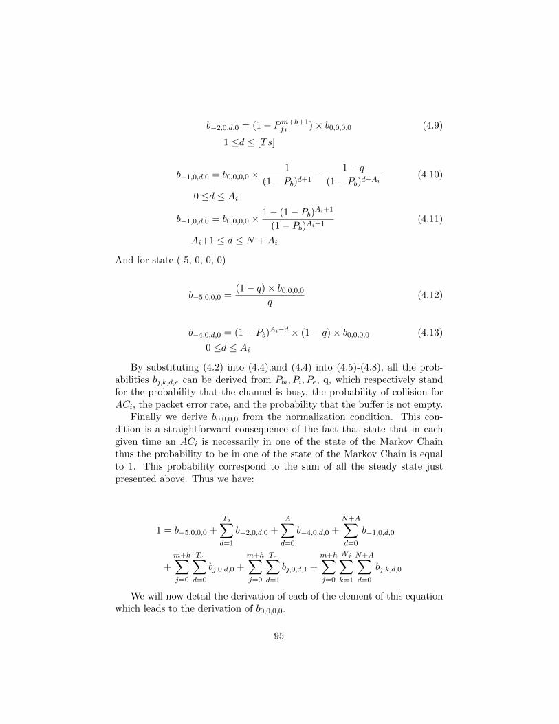
b−2,0,d,0 = (1− Pm+h+1fi )× b0,0,0,0 (4.9)

1 ≤d ≤ [Ts]

b−1,0,d,0 = b0,0,0,0 ×1

(1− Pb)d+1− 1− q

(1− Pb)d−Ai(4.10)

0 ≤d ≤ Ai

b−1,0,d,0 = b0,0,0,0 ×1− (1− Pb)Ai+1

(1− Pb)Ai+1(4.11)

Ai+1 ≤ d ≤ N +Ai

And for state (-5, 0, 0, 0)

b−5,0,0,0 =(1− q)× b0,0,0,0

q(4.12)

b−4,0,d,0 = (1− Pb)Ai−d × (1− q)× b0,0,0,0 (4.13)

0 ≤d ≤ Ai

By substituting (4.2) into (4.4),and (4.4) into (4.5)-(4.8), all the prob-abilities bj,k,d,e can be derived from Pbi, Pi, Pe, q, which respectively standfor the probability that the channel is busy, the probability of collision forACi, the packet error rate, and the probability that the buffer is not empty.

Finally we derive b0,0,0,0 from the normalization condition. This con-dition is a straightforward consequence of the fact that state that in eachgiven time an ACi is necessarily in one of the state of the Markov Chainthus the probability to be in one of the state of the Markov Chain is equalto 1. This probability correspond to the sum of all the steady state justpresented above. Thus we have:

1 = b−5,0,0,0 +

Ts∑d=1

b−2,0,d,0 +

A∑d=0

b−4,0,d,0 +

N+A∑d=0

b−1,0,d,0

+m+h∑j=0

Tc∑d=0

bj,0,d,0 +m+h∑j=0

Te∑d=1

bj,0,d,1 +m+h∑j=0

Wj∑k=1

N+A∑d=0

bj,k,d,0

We will now detail the derivation of each of the element of this equationwhich leads to the derivation of b0,0,0,0.

95

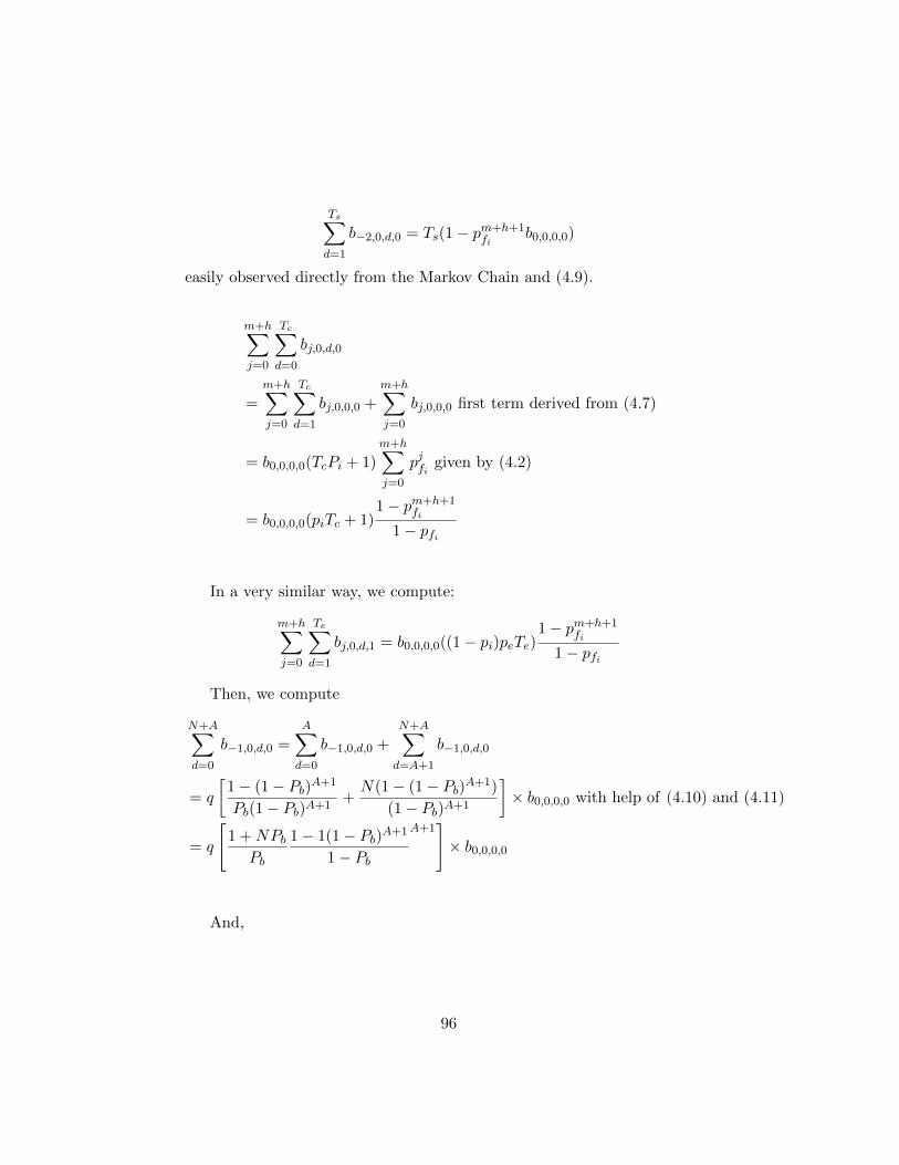
Ts∑d=1

b−2,0,d,0 = Ts(1− pm+h+1fi

b0,0,0,0)

easily observed directly from the Markov Chain and (4.9).

m+h∑j=0

Tc∑d=0

bj,0,d,0

=m+h∑j=0

Tc∑d=1

bj,0,0,0 +m+h∑j=0

bj,0,0,0 first term derived from (4.7)

= b0,0,0,0(TcPi + 1)m+h∑j=0

pjfi given by (4.2)

= b0,0,0,0(piTc + 1)1− pm+h+1

fi

1− pfi

In a very similar way, we compute:

m+h∑j=0

Te∑d=1

bj,0,d,1 = b0,0,0,0((1− pi)peTe)1− pm+h+1

fi

1− pfi

Then, we compute

N+A∑d=0

b−1,0,d,0 =

A∑d=0

b−1,0,d,0 +

N+A∑d=A+1

b−1,0,d,0

= q

[1− (1− Pb)A+1

Pb(1− Pb)A+1+N(1− (1− Pb)A+1)

(1− Pb)A+1

]× b0,0,0,0 with help of (4.10) and (4.11)

= q

[1 +NPb

Pb

1− 1(1− Pb)A+1

1− Pb

A+1]× b0,0,0,0

And,

96

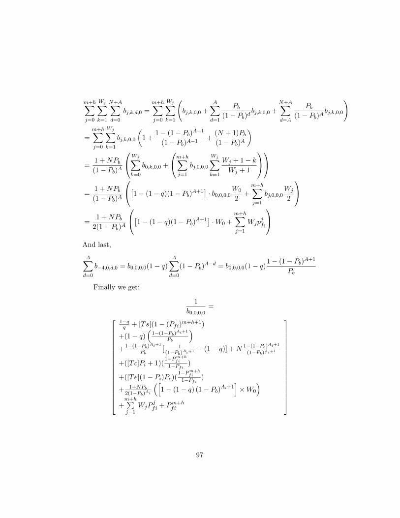
m+h∑j=0

Wj∑k=1

N+A∑d=0

bj,k,d,0 =m+h∑j=0

Wj∑k=1

(bj,k,0,0 +

A∑d=1

Pb(1− Pb)d

bj,k,0,0 +N+A∑d=A

Pb(1− Pb)A

bj,k,0,0

)

=

m+h∑j=0

Wj∑k=1

bj,k,0,0

(1 +

1− (1− Pb)A−1

(1− Pb)A−1+

(N + 1)Pb(1− Pb)A

)

=1 +NPb(1− Pb)A

Wj∑k=0

b0,k,0,0 +

m+h∑j=1

bj,0,0,0

Wj∑k=1

Wj + 1− kWj + 1

=

1 +NPb(1− Pb)A

[1− (1− q)(1− Pb)A+1]· b0,0,0,0

W0

2+

m+h∑j=1

bj,0,0,0Wj

2

=

1 +NPb2(1− Pb)A

[1− (1− q)(1− Pb)A+1]·W0 +

m+h∑j=1

Wjpjfi

And last,

A∑d=0

b−4,0,d,0 = b0,0,0,0(1− q)A∑d=0

(1− Pb)A−d = b0,0,0,0(1− q)1− (1− Pb)A+1

Pb

Finally we get:

1

b0,0,0,0=

1−qq + [Ts](1− (Pfi)

m+h+1)

+(1− q)(

1−(1−Pb)Ai+1

Pb

)+1−(1−Pb)Ai+1

Pb[ 1(1−Pb)Ai+1 − (1− q)] +N 1−(1−Pb)Ai+1

(1−Pb)Ai+1

+([Tc]Pi + 1)(1−Pm+h

fi

1−Pfi)

+([Te](1− Pi)Pe)(1−Pm+h

fi

1−Pfi)

+ 1+NPb

2(1−Pb)Ai

([1− (1− q) (1− Pb)Ai+1

]×W0

)+m+h∑j=1

WjPjfi + Pm+h

fi

97

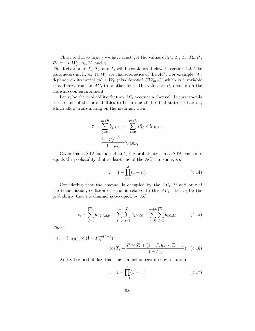
Thus, to derive b0,0,0,0 we have must get the values of Ts, Tc, Te, Pb, Pi,Pe, m, h, Wj , Ai, N, and q.The derivation of Ts, Tc, and Te will be explained below, in section 4.2. Theparameters m, h, Ai, N, Wj are characteristics of the ACi. For example, Wj

depends on its initial value W0 (also denoted CWmin), which is a variablethat differs from an ACi to another one. The values of Pe depend on thetransmission environment.

Let τi be the probability that an ACi accesses a channel. It correspondsto the sum of the probabilities to be in one of the final states of backoff,which allow transmitting on the medium, then:

τi =m+h∑j=0

bj,0,0,0i =m+h∑j=0

P ifi × b0,0,0,0i

=1− pm+h+1

fi

1− pfib0,0,0,0i

Given that a STA includes 4 ACi, the probability that a STA transmitsequals the probability that at least one of the ACi transmits, so:

τ = 1−3∏i=1

(1− τi) (4.14)

Considering that the channel is occupied by the ACi, if and only ifthe transmission, collision or error is related to this ACi. Let υi be theprobability that the channel is occupied by ACi

υi =

[Ts]∑d=1

b−2,0,d,0 +m+h∑j=0

[Tc]∑d=0

bj,0,d,0 +m+h∑j=0

[Te]∑d=1

bj,0,d,1 (4.15)

Then :

υi = b0,0,0,0i × (1− Pm+h+1fi )

× (Ts +Pi × Tc + (1− Pi)pe × Te + 1

1− Pfi) (4.16)

And υ the probability that the channel is occupied by a station

υ = 1−3∏i=1

(1− υi). (4.17)

98

The probability that the channel is busy is given by:

Pb = 1− (1− υ)M (4.18)

M stands for the total number of active stations. The collision probabilityis given by the probability that at least one other STA transmits at the sametime (called external collision) or an other ACi′ in the same STA (virtualinternal collision).

Pi = 1− (1− τ)M−1 ×∏i′>i

(1− τi′) (4.19)

(4.20)

And if we substitute by (4.14), we get:

Pi = 1−3∏j=0

(1− τj)M−13∏

j=i+1

1− τj (4.21)

where i’ means that ACi′ has a higher priority than ACi.

99

-5,0,0,0 = buffer empty

0,0,[Tc],0 = Collision

-1,0,0,0

0,W0,N+A,0 = Frozen

-2,0,[Ts],0 = Sending object

0,W0,0,0 = backoff

-4,0,A,0 = first try

0,0,0,0 = Transmit

-4,0,1,0

-1,0,N+A,0 = Frozen

0,1,0,0

0,1,N+A,0 = Frozen

1-q

q

1-q

Pb

1-Pb

1-Pb Pb Pb

(1-Pi)(1-Pe)

Pi

Pb

1-Pb

q

(1-Pb)/(W0+1)

0,0,[Te],1 = Error

(1-Pb)/(W0+1)

0,0, 1 ,0 0,0, 1 ,1

1,W0,N+A,0 = Frozen

1,W1,0,0 = backoff

1,1,0,0

1,1,N+A,0 = Frozen

1-Pb 1-Pb

(1-Pb)/(W0+1)

1,0,0,0 = Transmit

(1-Pi)Pe

1-Pb

Pb Pb

Rank: 1

m+h,0,0,0 = Transmit

Idem rank: 2 -> m, 1<j<m

and Wj+1 = 2Wj +1

Rank: 0

(1-Pi)(1-Pe)

1-q

q

(1-Pi)Pe+Pi

-2,0,1,0 = successful transmission

-2,0,[Ts]-1,0

-1,0,A,0

q

Idem rank: m -> m+h-1,m-1<j<m+h and Wj+1 = Wm

j,Wj,0,0 = backoff

j,Wm,0,0 = backoff

m+h,0,...,... = Collision and Error

j,0,0,0 = Transmit

j,0,0,0 = Transmit

Pb

-4,0,0,0

Figure 4.3: The full Markov chain

100

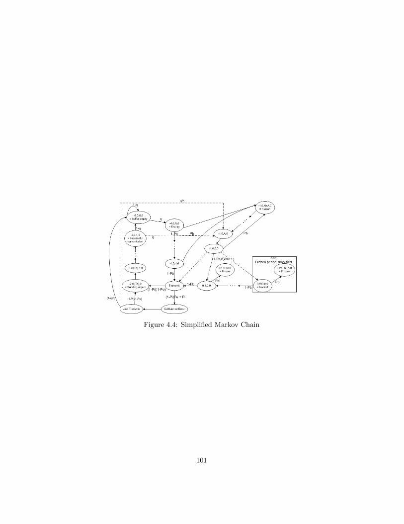
Figure 4.4: Simplified Markov Chain

101

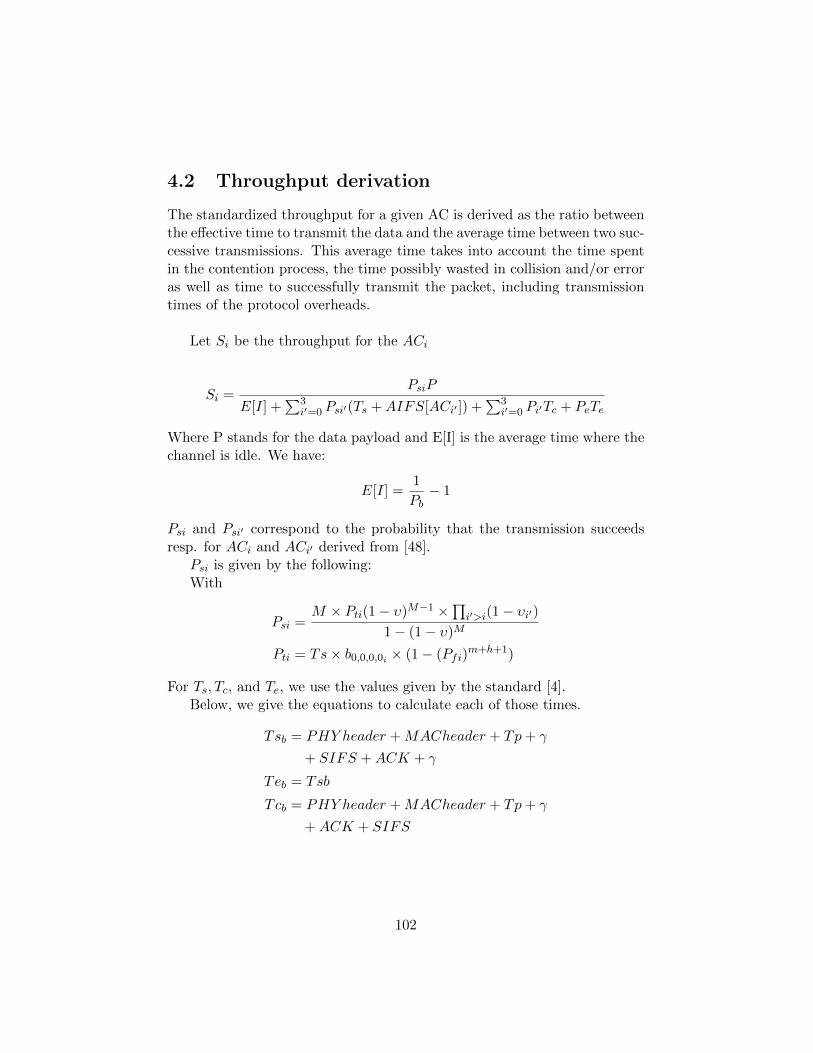
4.2 Throughput derivation

The standardized throughput for a given AC is derived as the ratio betweenthe effective time to transmit the data and the average time between two suc-cessive transmissions. This average time takes into account the time spentin the contention process, the time possibly wasted in collision and/or erroras well as time to successfully transmit the packet, including transmissiontimes of the protocol overheads.

Let Si be the throughput for the ACi

Si =PsiP

E[I] +∑3

i′=0 Psi′(Ts +AIFS[ACi′ ]) +∑3

i′=0 Pi′Tc + PeTe

Where P stands for the data payload and E[I] is the average time where thechannel is idle. We have:

E[I] =1

Pb− 1

Psi and Psi′ correspond to the probability that the transmission succeedsresp. for ACi and ACi′ derived from [48].

Psi is given by the following:With

Psi =M × Pti(1− υ)M−1 ×

∏i′>i(1− υi′)

1− (1− υ)M

Pti = Ts× b0,0,0,0i × (1− (Pfi)m+h+1)

For Ts, Tc, and Te, we use the values given by the standard [4].Below, we give the equations to calculate each of those times.

Tsb = PHY header +MACheader + Tp+ γ

+ SIFS +ACK + γ

Teb = Tsb

Tcb = PHY header +MACheader + Tp+ γ

+ACK + SIFS

102

And for the RTS/CTS mode:

Tsr = RTS + γ + SIFS + CTS + γ

+ SIFS + PHY header +MACheader

+ Tp+ γ + SIFS +ACK + γ

Ter = Tsr

Tcr = RTS + γ + SIFS + CTS + γ

+ SIFS

Where Tp stands for the payload’s transmission time which obviously de-pends on the nominal throughput R (e.g.: 11 Mbps for 802.11b).

4.3 Delay derivation

In this section we compute the delay encountered by a single station. Bydelay we mean the amount of time required from the moment the packetarrive at the top of the buffer till it’s successfully transmitted. By successfultransmission we assume also the reception of an ACK. This later supplemen-tary time period is taken into account in the Tsb (or Tsr) time computedabove. As our model extends the one developed by [48], the way we com-pute the delay is naturally similar. However , because we have an additionaldimension, some other states have to be accounted for in the final calcula-tion. The delay is computed in a recursive manner. For instance the delayat state (j, k, d, e) denoted Dj,k,d,e stands for the delay the sta waits fromthe time the packet was delivered at the top of the buffer till it arrives atstate (j, k, d, e). For example to compute the delay Dj,k,A+1,0, we know thatthe transition probability from state Dj,k,A,0 is 1. Thus we can state thatDj,k,A,0 = Dj,k,A+1,0 +1, in other words the delay at state (j, k, A, 0) is equalto the delay accumulated at (j, k, A+ 1) + 1. As the probability to arrive ata given states is sometimes more complex as we saw in 4.1.4, the delay inrespectively more complex. We assume in the following that all steady stateprobabilities are known and computed as in 4.1.5. If we assume Dj,k−1,d,e isknown, the relationships between states (j, k − 1, 0, e) and (j, k, d, e) whend = 0, 1, 2...., N +A, are

103

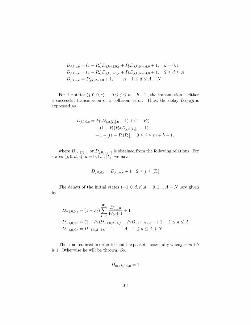
Dj,k,d,e = (1− Pb)Dj,k−1,0,e + PbDj,k,N+A,0 + 1, d = 0, 1

Dj,k,d,e = (1− Pb)Dj,k,d−1,e + PbDj,k,N+A,0 + 1, 2 ≤ d ≤ ADj,k,d,e = Dj,k,d−1,0 + 1, A+ 1 ≤ d ≤ A+N

For the states (j, 0, 0, e), 0 ≤ j ≤ m+h−1 , the transmission is eithera successful transmission or a collision, error. Thus, the delay Dj,0,0,0 isexpressed as

Dj,0,0,e = Pi(Dj,0,[Tc],0 + 1) + (1− Pi)+ (1− Pi)Pe(Dj,0,[Te],1 + 1)

+ 1− [(1− Pi)Pe], 0 ≤ j ≤ m+ h− 1.

where Dj,o,[Tc],0 or Dj,0,[Te],1 is obtained from the following relations. Forstates (j, 0, d, e), d = 0, 1..., [Te] we have

Dj,0,d,e = Dj,0,d,e + 1 2 ≤ j ≤ [Te]

The delays of the initial states (−1, 0, d, e),d = 0, 1..., A + N ,are givenby

D−1,0,0,e = (1− Pb)W0∑k=0

D0,k,0

W0 + 1+ 1

D−1,0,d,e = (1− Pb)D−1,0,d−1,f + PbD−1,0,N+A,0 + 1, 1 ≤ d ≤ AD−1,0,d,e = D−1,0,d−1,0 + 1, A+ 1 ≤ d ≤ A+N

The time required in order to send the packet successfully whenj = m+his 1. Otherwise he will be thrown. So,

Dm+h,0,0,0 = 1

104

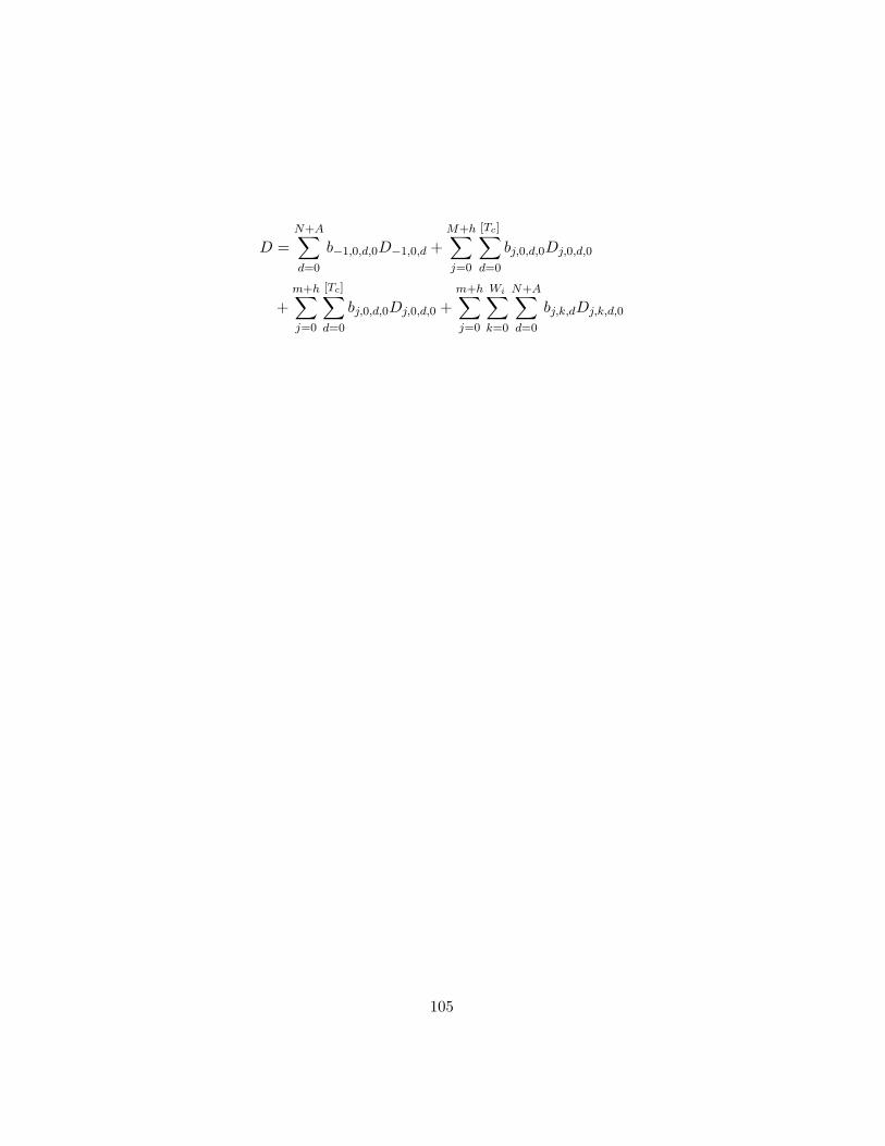
D =N+A∑d=0

b−1,0,d,0D−1,0,d +M+h∑j=0

[Tc]∑d=0

bj,0,d,0Dj,0,d,0

+

m+h∑j=0

[Tc]∑d=0

bj,0,d,0Dj,0,d,0 +

m+h∑j=0

Wi∑k=0

N+A∑d=0

bj,k,dDj,k,d,0

105

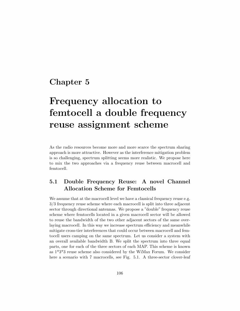
Chapter 5

Frequency allocation tofemtocell a double frequencyreuse assignment scheme

As the radio resources become more and more scarce the spectrum sharingapproach is more attractive. However as the interference mitigation problemis so challenging, spectrum splitting seems more realistic. We propose hereto mix the two approaches via a frequency reuse between macrocell andfemtocell.

5.1 Double Frequency Reuse: A novel ChannelAllocation Scheme for Femtocells

We assume that at the macrocell level we have a classical frequency reuse e.g.3/3 frequency reuse scheme where each macrocell is split into three adjacentsector through directional antennas. We propose a ”double” frequency reusescheme where femtocells located in a given macrocell sector will be allowedto reuse the bandwidth of the two other adjacent sectors of the same over-laying macrocell. In this way we increase spectrum efficiency and meanwhilemitigate cross-tier interferences that could occur between macrocell and fem-tocell users camping on the same spectrum. Let us consider a system withan overall available bandwidth B. We split the spectrum into three equalparts, one for each of the three sectors of each MAP. This scheme is knownas 1*3*3 reuse scheme also considered by the WiMax Forum. We considerhere a scenario with 7 macrocells, see Fig. 5.1. A three-sector clover-leaf

106

cellular layout is used. We use 3 colors: B: Blue, R: Red and G: Green torepresent the 3 parts of the split spectrum. For each sector, we allow thefemtocells in it to reuse the spectrum not used by its MAP (i.e. two-thirdsof the available bandwidth). We propose three kinds of reuse plans:

• Full reuse: The simplest reuse plan is full reuse over the whole area.This means that wherever the femtocell is located on the area of itssector it can reuse whatever frequency used by the two adjacent sectors.The selection by each femtocell of a specific frequency among thosespectra will be detailed in section y5.2. The advantage of this reusemethod is that more channels are available for femtocells, thus moreflexibility to mitigate inter-femtocell interferences. The drawback ofthis method is that problems might occur when the FAP is close to theedge of the sector. Assume that the FAP chooses the same frequencythat the adjacent macrocell sector, then it can suffer from Macrocellinterference of the sector using the same spectrum in the adjacentcell in downlink, and vice versa ”attack” the macrocell uplink as weexplained in section 3.3.

• Partial reuse: The second method to share the spectrum of the ad-jacent sectors between FAPs is to split the sector into 6 equal partsconsidering our example but without loss of generality. Then we allo-cate to each part, the spectrum that is not used by the nearest sectorof the adjacent cell. We avoid here the problem induced by the fullreuse scheme but on the other hand the pool of frequencies that can bechosen by neighboring femtocells is reduced. This can lead to severeco-tier interference in case of a dense femtocell population.

• Mixed reuse: In this third method we try to find a tradeoff which helpsus in keeping the advantages of the two previous methods. We definethe central region where both adjacent sectors spectra can be usedas in the full reuse, and the cell boundary region where, as in partialreuse method, only the spectrum not used by the nearest sector can beused. For this method we can define the radius of the central regionin a static or dynamic manner. For the dynamic radius we have touse an algorithm that computes it, based on statistics of interferenceof Macro-to-Femto and vice-versa, at the boundary. If interferencedecreases, e.g. because of less loaded MAP edge, then we can extendthe central region.

107

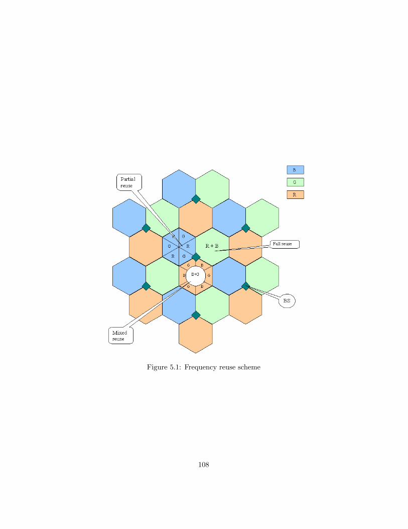
Figure 5.1: Frequency reuse scheme

108

5.2 Femtocell’s Channel Selection

In this section we deal with the issue of sharing radio resources among theFAPs. Even though at the macrocell level, resource allocation can be sched-uled by some complex central algorithm, the femtocell specifications requirean auto-configuration mechanism. Given the large number of femtocells thatcould be deployed in a given area, especially in an urban environment, andthe lack of a central coordinator a priori, channel assignments seem to bevery complex. To avoid transmitting large amounts of information to a cen-tralized scheduler and to avoid complexity issues from the processing of largeamounts of information, we need to use an auto-configuration mechanism.This issue is currently under intensive research and standardization effortsunder the terms such as: Spectrum Sensing, Cognitive Radio and Self Or-ganizing Networks . We propose here a simple approach. The FAP sensesthe available spectrum and selects the subchannels that are not currentlybeing used, if there are such subchannels. Then it sends to the user the listof the subchannels and the user senses each of them for a given time andthen sends a feedback through Channel State Information (CSI) report foreach subchannel. The subchannels which offer the best channel conditionin terms of SINR is then chosen by the FAP. If no free subchannel is avail-able, the FAP selects the least interfered subchannel, i.e. the subchannel inwhich the Received Signal Strength (RSS)(of the interference signals) is thelowest. It can ensure that the future transmission wont degrade the ongoingtransmission. In this case, we could also take into account load statistics ofeach subchannel to improve the selection since a lightly loaded subchannelcould perform better than a heavily loaded channel but with higher RSS.We assumed here that all the subchannels have equal bandwidth. Howeverit might not be the case and thus channel selection may be more complex.

5.3 Other Fundamentals Parameters

In this section we deal with some other parameters we have to take into ac-count in our proposal. For instance, we have to define what radio resourcegranularity will be considered in our model, as it could have some implica-tions on the results. Moreover for the deployment scenarios considered, thetransmission power at both the macro and femto level are fundamental pa-rameters also have to be defined. Finally channel models and access controlto the femtocell are detailed.

109

5.3.1 Radio Resource Granularity

Before starting the process of channel selection as presented in the section5.1 we must define what will be the resource forming a channel or in otherwords, given the spectrum that can be reused by femtocells, how much of itwill be granted to each femtocell.

The transmission technique we consider is OFDM, and the multiple ac-cess technique is OFDMA. Thus a resource unity is defined as a set of sub-carriers over a given time period. This also referred as Resource Block (RB) in LTE. We assume here the use of FDD although TDD is also defined by3GPP LTE.

The granularity is defined both on frequency and time domains but wedo not consider here the latter. We explain in the next paragraph whatmotivate this consideration .

We will describe in the following the tradeoff involved in the granularityof the frequency domain.

Available subcarriers may be grouped into subchannels. This division(number of subcarriers per subchannel) is not easy to define.

On the one hand the more subcarriers per channel, the more bandwidthavailable to each femtocell and thus the more available capacity per user. Inthis case the femtocell can benefit from frequency diversity which leads tomore efficient communications, especially if subcarriers composing a chan-nel are spread out over the entire bandwidth a.k.a distributed subcarrierpermutation (see further).

On the other hand, with fewer subcarriers per channel more channels aremade available for different femtocell and thus there will be less cochannelinterference between femtocells, as each one will be able to get its ownsubschannel which will be orthogonal to the others. However in this case, thesensibility to frequency offset will be higher than in the previous case and willrequire strong frequency synchronization, because the frequency distancebetween two subchannels will be smaller.Moreover the OFDM diversity gain,and resistance to frequency-selective fading, may partly be lost if very fewsub-carriers are assigned to each user, and if the same carrier is used in everyOFDM symbol [12].Adaptive sub-carrier assignment based on fast feedbackinformation about the channel, and/or sub-carrier frequency hopping, istherefore desirable.In addition, flexible allocation of subchannels can be usedto dynamically allocate bandwidth to individual users for various bit rateservices

In brief, we must consider the following questions:

1. How many subcarriers will be allocate to each sub channel?

110

2. will these subcarriers be contiguous or distributed over the whole avail-able spectrum?

3. How many subchannel will be allocated to each user?

4. Will these allocations be dynamic or static?

In fact the issue of ”subchannelization” i.e. number of subcarriers persubchannel and resource allocation i.e. number of subchannel per user is tobe considered as a full problem and is beyond the scope of our proposition.Thus we will content ourselves with a simple approach where the numberof subcarriers per subchannel will be fixed and equal for each subchannel,and the number of subchannels per user will also be fixed and equal for eachuser.

Distributed or Contiguous Subcarriers Allocation

Subchannels may be constituted using either contiguous subcarriers or sub-carriers pseudorandomly distributed across the frequency spectrum. Sub-channels formed using distributed subcarriers provide more frequency di-versity, which is particularly useful for mobile applications. The subchan-nelization scheme based on contiguous subcarriers is called (in WiMAX)Adaptive Modulation and Coding (AMC). Although frequency diversity islost, AMC allows system designers to exploit multiuser diversity, allocatingsubchannels to users based on their frequency response. Multiuser diversitycan provide significant gains in overall system capacity, if the system strivesto provide each user with a subchannel that maximizes its received SINR. Ingeneral, contiguous subchannels are more suited for fixed and low-mobilityapplications.

Besides an advantage of contiguous allocation is the reduction of Adja-cent Channel Interference (ACI). This is particularly relevant if each subcar-rier bandwidth is small. It is a meaningful advantage of contiguous allocationsince ACI is likely to happen at the femtocell level as very close coexistencebetween users of different cells can occur.

Time domain granularity

We describe here briefly the issue of time domain granularity for femtocell.In a very bad environment, frequency diversity could be critical. But as

mentioned if the femtocells population is dense lack of sufficient channelswould lead to strong cochannel interference. In such a case it could be

111

interesting to share the resource also on a time basis, i.e. the resource unityto be granted to each femtocell will not be based only on subcarriers butalso on time unity of resource use. An obvious drawback of this methodis the strong requirement of time synchronization. Besides a challengingpoint would be time coordination, which seems impossible regarding thenumber of femtocells that can be deployed in a given area. The only wayto allocate the resource of a same channel on a time basis without centralcoordination would be the use of the famous CSMA/CA technique used inWifi [1] networks which would lead to really poor performance when numberof user increase.

Another option would be the usage of clusters. All the femtocells thatselect the same channel form a cluster. From this cluster we need to extracta cluster’s head which will have to coordinate the transmission of each of thefemtocell. In this way we avoid the problem of complex coordination but wego back to the famous problem of self organization that we meet in ad hocnetwork, which bring us among other things to the issue of which head tochoose given requirement of high computation capability. We need also tosolve some security issue, avoiding a malicious user’s being the coordinatorand keeping all the resource. However in this option we could make useof QoS principle to grant priority to delay sensitive traffic between severalfemtocells as in WiMax resource Granting rules.

5.3.2 Femtocell Transmission Power

In the previous sections we defined what will the radio resources availableto each femtocell be. Now, we present what has to be the transmissionpower of FAPs, and Femtocell User Equipments (FUEs). Power is one ofthe key parameters of the problem since a good and accurate tuning of thetransmission power will avoid interference outside the femtocell and thusallow an efficient reuse of the bandwidth. The configuration of the trans-mission power requires taking into account several parameters: Modulationand coding scheme (the higher the modulation scheme the higher the powerrequired maintaining a given BER), the subchannel bandwidth (at a givendata rate increasing bandwidth allow decreasing transmission power whatwe can easily conclude from Shannon’s capacity formula [60]), and the chan-nel model. The transmission power has to be set to a value that is on averageequal to the power received from the ”strongest” co-channel Macrocell plusthe required power to cover the entire femtocell area [26]. This process hasto be performed periodically to ensure power control, since the network isdynamic and new Macro users or femtocells can appear or disappear.For the

112

purpose of the simulation, we propose in a first step to fix the transmissionpower both downlink and uplink. The transmission power will be set to the”classical” value allowed by the 3GPP specifications.

5.3.3 Adjacent Channel Interference

We must mention that we didn’t find yet a way to account for the Adja-cent Channel Interference (ACI). We briefly develop here this issue that isconsidered here as a valuable future work.

Orthogonality is one of the most valuable features of OFDM, so impor-tant that it even gives the name to this transmission technique. Howeverwhen using OFDMA and thus sharing the same OFDM symbol betweenmultiple senders, orthogonality can not longer be guaranteed by construc-tion. Fully synchronized coherent transmission between users is currentlyhard to imagine and until proof of feasibility the assumption of uncorrelatedsenders must hold. Thus the ACI of the Adjacent Channel Leakage powerRatio (ACLR) from the femtocell BS, the mobile station tx and the Adja-cent Channel Selectivity (ACS) of the femtocell BS, mobile station receiversneed to be taken into account. In order to measure ACLR it is necessaryto consider a measurement filter for the transmitted signal as well as a re-ceiver measurement bandwidth for the adjacent channel (”victim”) system.ACLR can be mitigated by mean of the guard band already used in theOFDM symbol. In some cases the number/size of the guard band shouldbe enlarged to increase protection from the interfering side-band transmis-sion power of adjacent channels. Therefore there will be a tradeoff betweenincreased protection through guard bands and increased capacity which re-quires less unused subcarriers. It is worth mentioning that the problem iseven worse for femtocells where this phenomenon occurs both in Uplink (UL)and Downlink (DL) in contrast to macrocells where it is likely to happenonly in UL.

Similar scenarios occur when two different systems coexist in the samefrequency band, such as 802.16 and CDMA-DS of IMT-2000. In some casesisolation of about 10 dB can be required to avoid severe degradations evenfor second adjacent channels. Given the transmitted powers, path losses inthe selected scenarios and the ACLR and ACS performances of the basestations, SubStations ( in WiMAX) and mobile stations in each system, theeffective interference may be calculated.

113

Part III

Results

114

Chapter 6

Analytical Results of theStochastic Model of EDCA

In this chapter, we present the results of our analytical model. The param-eters used in the model are summarized in Table 6.1. If not specified, weassume in the following scenarios that default parameters (cf. Table 6.1) areused. We derived the throughput for an IEEE 802.11b infrastructure cellwith the basic EDCA scheme. The study of IEEE 802.11a is straightforwardsince it is just required to change the data rate and some parameters spe-cific to this standard. Besides, RTS/CTS can be modeled simply by takinginto account Tcr instead of Tcb in the collision time where Tcr stands forthe collision of the RTS/CTS packet only. Before presenting the results webriefly outline in which way we compute our model

6.1 Equations System

In this section we describe how we solve our model and retrieve analyticalresults. As we saw in section 4.1.5, all the steady state probability rely onlyon b0,0,0,0. To compute the b0,0,0,0 we need also Pi etc... Thus to derivethroughput and delay we need:

115

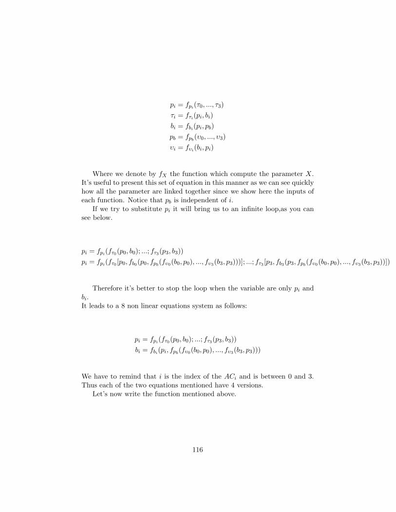
pi = fpi(τ0, ..., τ3)

τi = fτi(pi, bi)

bi = fbi(pi, pb)

pb = fpb(υ0, ..., υ3)

υi = fυi(bi, pi)

Where we denote by fX the function which compute the parameter X.It’s useful to present this set of equation in this manner as we can see quicklyhow all the parameter are linked together since we show here the inputs ofeach function. Notice that pb is independent of i.

If we try to substitute pi it will bring us to an infinite loop,as you cansee below.

pi = fpi(fτ0(p0, b0); ...; fτ3(p3, b3))

pi = fpi(fτ0 [p0, fb0(p0, fpb(fυ0(b0, p0), ..., fυ3(b3, p3)))]; ...; fτ3 [p3, fb3(p3, fpb(fυ0(b0, p0), ..., fυ3(b3, p3))])

Therefore it’s better to stop the loop when the variable are only pi andbi.It leads to a 8 non linear equations system as follows:

pi = fpi(fτ0(p0, b0); ...; fτ3(p3, b3))

bi = fbi(pi, fpb(fυ0(b0, p0), ..., fυ3(b3, p3)))

We have to remind that i is the index of the ACi and is between 0 and 3.Thus each of the two equations mentioned have 4 versions.

Let’s now write the function mentioned above.

116

fp0(a, b, c, d) = 1− [(1− a)M−1(1− b)M (1− c)M (1− d)M ]

fp1(a, b, c, d) = 1− [(1− a)M−1(1− b)M−1(1− c)M (1− d)M ]

fp2(a, b, c, d) = 1− [(1− a)M−1(1− b)M−1(1− c)M−1(1− d)M ]

fp3(a, b, c, d) = 1− [(1− a)M−1(1− b)M−1(1− c)M−1(1− d)M−1]

fτi(ai, bi) = [1− (pe + (1− pe)ai)m+h+1

(1− pe)(1− ai)]bi

fbi(ai, b) = [1− qq

+ [Ts](1− (pe + (1− pe)ai)m+h+1)

+ (1− q)(1− (1− b)A+1

b) + q

(1 +N.b)

b

1− (1− b)A+1

(1− b)A+1

+ ([Tc]ai + 1)(1− pm+h+1

fi

1− pfi) + ([Te](1− pi)pe)(

1− (pe + (1− pe)ai)m+h+1

(1− pe)(1− ai))

+1 +N.b

2(1− b)A([1− (1− q)(1− b)A+1]W0

+m+h∑j=1

Wj(pe + (1− pe)ai)j) + (pe + (1− pe)ai)m+h]−1

fpb(a, b, c, d) = 1− (1− a)M (1− b)M (1− c)M (1− d)M

fυi(bi, ai) = bi(1− (pe + (1− pe)ai)m+h+1)[Ts +aiTc + (1− ai)peTe + 2

(1− pe)(1− ai)]

All those function were calculated in Matlab. In the following sectionwe detail the results obtained.

It is worth mentioning that we first tried to solve this set of non linearequations using the fixed point theorem. This method is a well knownnumerical method to solve non linear equations. However at the end of ourmathematical analysis we needed to pose a validity condition for convergencewhich was Pe → 1 which was not realistic. Thus we abandoned this method.Regardless, we decided to include in the appendix the development of this

117

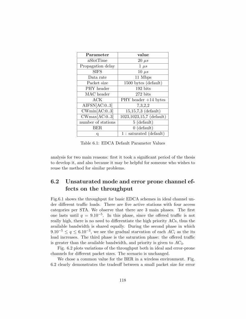
Parameter value

aSlotTime 20 µs

Propagation delay 1 µs

SIFS 10 µs

Data rate 11 Mbps

Packet size 1500 bytes (default)

PHY header 192 bits

MAC header 272 bits

ACK PHY header +14 bytes

AIFSN[AC:0..3] 7,3,2,2

CWmin[AC:0..3] 15,15,7,3 (default)

CWmax[AC:0..3] 1023,1023,15,7 (default)

number of stations 5 (default)

BER 0 (default)

q 1 : saturated (default)

Table 6.1: EDCA Default Parameter Values

analysis for two main reasons: first it took a significant period of the thesisto develop it, and also because it may be helpful for someone who wishes toreuse the method for similar problems.

6.2 Unsaturated mode and error prone channel ef-fects on the throughput

Fig.6.1 shows the throughput for basic EDCA schemes in ideal channel un-der different traffic loads. There are five active stations with four accesscategories per STA. We observe that there are 3 main phases. The firstone lasts until q = 9.10−5. In this phase, since the offered traffic is notreally high, there is no need to differentiate the high priority ACs, thus theavailable bandwidth is shared equally. During the second phase in which9.10−5 ≤ q ≤ 6.10−3, we see the gradual starvation of each ACi as the itsload increases. The third phase is the saturation phase: the offered trafficis greater than the available bandwidth, and priority is given to AC3.

Fig. 6.2 plots variations of the throughput both in ideal and error-pronechannels for different packet sizes. The scenario is unchanged.

We chose a common value for the BER in a wireless environment. Fig.6.2 clearly demonstrates the tradeoff between a small packet size for error

118

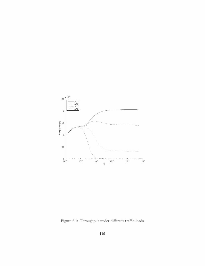
10−5

10−4

10−3

10−2

10−1

100

0

0.5

1

1.5

2

2.5x 10

6

q

Thr

ough

put (

bps)

AC3AC2AC1AC0

Figure 6.1: Throughput under different traffic loads

119

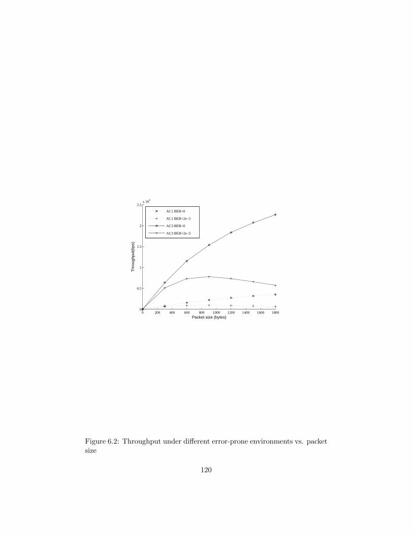
0 200 400 600 800 1000 1200 1400 1600 18000

0.5

1

1.5

2

2.5x 10

6

Packet size (bytes)

Thr

ough

put(

bps)

AC1 BER=0

AC1 BER=2e−5

AC3 BER=0

AC3 BER=2e−5

Figure 6.2: Throughput under different error-prone environments vs. packetsize

120

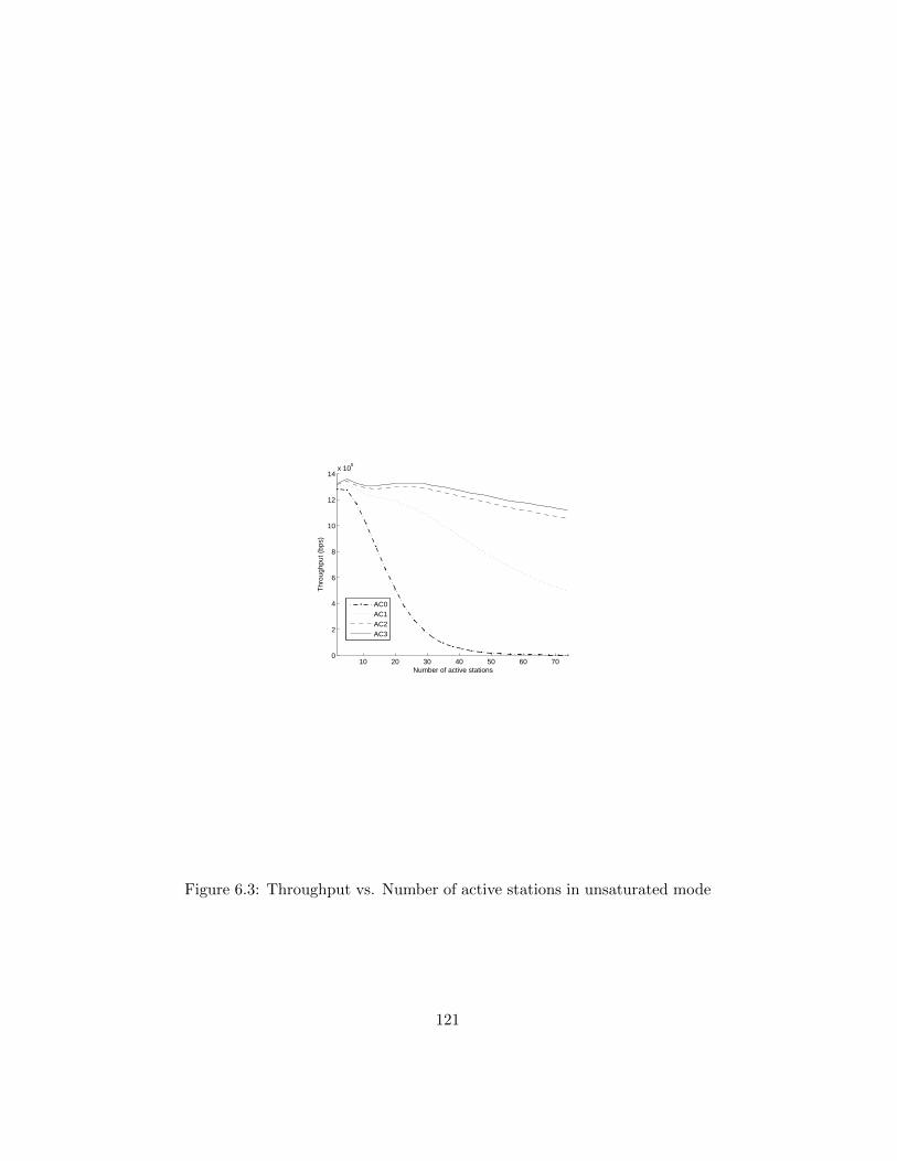
10 20 30 40 50 60 700

2

4

6

8

10

12

14x 10

5

Number of active stations

Thr

ough

put (

bps)

AC0AC1AC2AC3

Figure 6.3: Throughput vs. Number of active stations in unsaturated mode

121

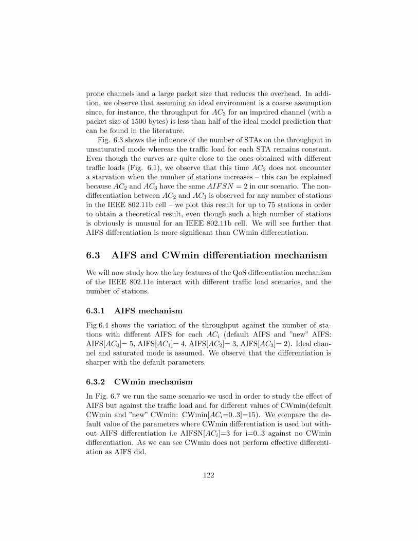
prone channels and a large packet size that reduces the overhead. In addi-tion, we observe that assuming an ideal environment is a coarse assumptionsince, for instance, the throughput for AC3 for an impaired channel (with apacket size of 1500 bytes) is less than half of the ideal model prediction thatcan be found in the literature.

Fig. 6.3 shows the influence of the number of STAs on the throughput inunsaturated mode whereas the traffic load for each STA remains constant.Even though the curves are quite close to the ones obtained with differenttraffic loads (Fig. 6.1), we observe that this time AC2 does not encountera starvation when the number of stations increases – this can be explainedbecause AC2 and AC3 have the same AIFSN = 2 in our scenario. The non-differentiation between AC2 and AC3 is observed for any number of stationsin the IEEE 802.11b cell – we plot this result for up to 75 stations in orderto obtain a theoretical result, even though such a high number of stationsis obviously is unusual for an IEEE 802.11b cell. We will see further thatAIFS differentiation is more significant than CWmin differentiation.

6.3 AIFS and CWmin differentiation mechanism

We will now study how the key features of the QoS differentiation mechanismof the IEEE 802.11e interact with different traffic load scenarios, and thenumber of stations.

6.3.1 AIFS mechanism

Fig.6.4 shows the variation of the throughput against the number of sta-tions with different AIFS for each ACi (default AIFS and ”new” AIFS:AIFS[AC0]= 5, AIFS[AC1]= 4, AIFS[AC2]= 3, AIFS[AC3]= 2). Ideal chan-nel and saturated mode is assumed. We observe that the differentiation issharper with the default parameters.

6.3.2 CWmin mechanism

In Fig. 6.7 we run the same scenario we used in order to study the effect ofAIFS but against the traffic load and for different values of CWmin(defaultCWmin and ”new” CWmin: CWmin[ACi=0..3]=15). We compare the de-fault value of the parameters where CWmin differentiation is used but with-out AIFS differentiation i.e AIFSN[ACi]=3 for i=0..3 against no CWmindifferentiation. As we can see CWmin does not perform effective differenti-ation as AIFS did.

122

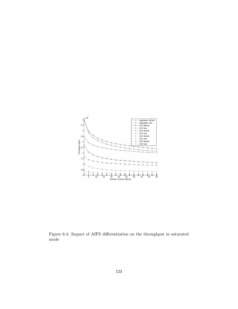
5 10 15 20 25 30 35 40 45 500

0.5

1

1.5

2

2.5

3

3.5

4

4.5

5x 10

6

Number of active stations

Thr

ough

put (

bps)

aggregate: defaultaggregate: newAC3 defaultAC3 newAC2 defaultAC2 newAC1 defaultAC1 newAC0 defaultAC0 new

Figure 6.4: Impact of AIFS differentiation on the throughput in saturatedmode

123

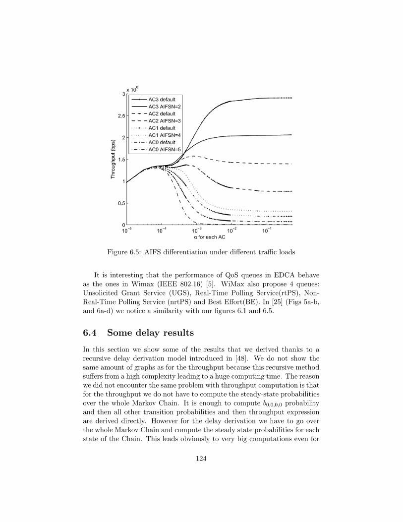
Figure 6.5: AIFS differentiation under different traffic loads

It is interesting that the performance of QoS queues in EDCA behaveas the ones in Wimax (IEEE 802.16) [5]. WiMax also propose 4 queues:Unsolicited Grant Service (UGS), Real-Time Polling Service(rtPS), Non-Real-Time Polling Service (nrtPS) and Best Effort(BE). In [25] (Figs 5a-b,and 6a-d) we notice a similarity with our figures 6.1 and 6.5.

6.4 Some delay results

In this section we show some of the results that we derived thanks to arecursive delay derivation model introduced in [48]. We do not show thesame amount of graphs as for the throughput because this recursive methodsuffers from a high complexity leading to a huge computing time. The reasonwe did not encounter the same problem with throughput computation is thatfor the throughput we do not have to compute the steady-state probabilitiesover the whole Markov Chain. It is enough to compute b0,0,0,0 probabilityand then all other transition probabilities and then throughput expressionare derived directly. However for the delay derivation we have to go overthe whole Markov Chain and compute the steady state probabilities for eachstate of the Chain. This leads obviously to very big computations even for

124

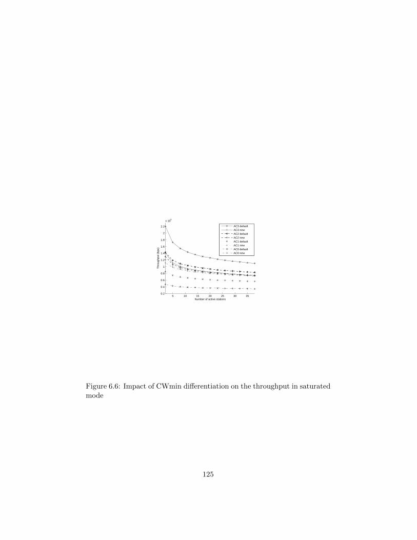
5 10 15 20 25 30 350.2

0.4

0.6

0.8

1

1.2

1.4

1.6

1.8

2

2.2

x 106

Number of active stations

Thr

ough

put (

bps)

AC3 defaultAC3 newAC2 defaultAC2 newAC1 defaultAC1 newAC0 defaultAC0 new

Figure 6.6: Impact of CWmin differentiation on the throughput in saturatedmode

125

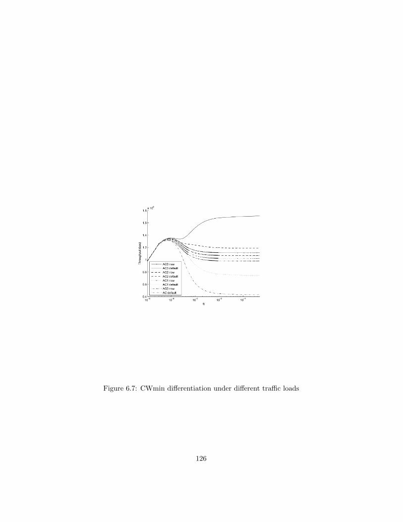
Figure 6.7: CWmin differentiation under different traffic loads

126

small numbers of stations. In the framework of our future work we havealready begun ,we are developing heuristic methods usually used for solvingmultidimensional markov chains. We expect that the processing time willthen decrease significantly. In Fig. 6.8 we observe the effect of the numberof stations connected to the AP on the delay experienced by each STA. Wenotice the efficiency of the differentiation mechanism which gives priority toAC1. When we are close to the saturation point, the delay increases evenfor AC1 due to the high number of collisions. Unlike the previous case, inFig. 6.9 if we consider only 5 STAs, the differentiation mechanism is efficienteven when the traffic load increases. This is because when the number ofstations is fixed, increasing the traffic load does not lead to an increase ofthe collision probability.

127

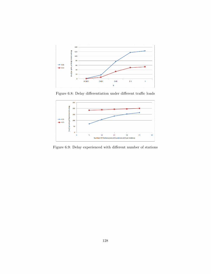
Figure 6.8: Delay differentiation under different traffic loads

Figure 6.9: Delay experienced with different number of stations

128

Chapter 7

Simulation and Results forFemtocell Channels Reuse

In this chapter we present the performances achieved by the schemes pro-posed in Chap. 5. In the next section we present the indicators we chooseto assess the performance of femtocells. Then we show the simulator wedeveloped for the purpose of our research. Finally the results obtained fromdifferent scenarios are presented.

7.1 Performance derivation

In this section we present the different indicators we used to derive the per-formance of the femtocells. First of all, we use the Received Signal Strength(RSS). It stands for the signal power received in a given device. If for exam-ple we consider the femtocell downlink case, then the RSS will be the signalpower received by the Femtocell User Equipment (FUE) from its servingFemtocell Access Point (FAP). To compute the RSS we need to subtractfrom the transmitted power (e.g. here at the FAP), the propagation loss ofthe signal. Propagation loss depend on the propagation models used whichwe discuss further in 7.2.1. We have to note here that RSS does not takeinto account the interference of the different users transmitting at the sametime on the same channel. Even if Shannon’s Capacity [59] formula is notlinked to RSS, this indicator is still interesting. The reason is that evenif we consider a device ”ideally” alone with its serving Access Point (AP)thus without interference from outside, if the RSS is very low, the receiv-ing device will not be able to decode correctly the signal. Thus in everydevice, a parameter called ”receiver sensitivity” defines what is the mini-

129

mum level of RSS required to be able to provide a minimum service. In thecontext of femtocells and macrocells, this indicator is especially importantsince propagation loss are somewhat different in each layer. When FUE isconnected through the Macrocell Access Point (MAP) the penetration lossdue to walls, windows etc... can lead to outages due to lower RSS thanreceiver sensitivity. This problem is often more critical in downlink than inuplink, because User Equipment (UE) are often limited in the quality of theelectronics inside due to price constraints and battery consumption whereasthis can be leveraged when dealing with AP.

The second indicator we used in the following is the Signal to Interferenceand Noise Ratio (SINR) also called Carrier to Interference and Noise Ratio(CINR). It is important to distinguish this indicator from the Signal toNoise Ratio (SNR). In the latter we only take into account the thermal noiseinherent to every electronic component and that depends on the temperatureand the bandwidth of the channel we transmit over. Unlike SNR, in SINRwe also take into account the interferences due to simultaneous transmissionsover the same channel from other UEs or APs. As indicated by its namethe SINR accounts for the ratio of the RSS to the thermal noise level andthe outside interferences. Unlike RSS, the derivation of SINR is differentwhether it is for the downlink or the uplink.

In downlink the interference is from the APs whereas in the uplink theinterference is from other UEs. Thus for example when we compute thedownlink SINR at the FUE we first compute the RSS from its serving FAP,and then we divide this value by RSSs from other MAPs and FAPs that aretransmitting on the same channel and the thermal noise at the FUE.

In addition to the computation of SINRs we made the following assump-tions. For the downlink we investigated 3 tiers of interfering MAPs whereasfor the uplink case we consider interferences only from the MUEs located inthe same cell as the FAPs or MAP where we compute the SINR . Moreoverwe do not consider FAPs and FUEs in adjacent cells since the penetrationloss attenuates their already low transmitted powers under a negligible level.

7.2 Simulation Parameters

As a worst case scenario for femtocells capacity, we investigate several net-work configurations in a very dense urban environment. Furthermore, incomparison with real networks, we assume relatively high macro transmitpowers without modeling power control and DTX for interference reduction.

130

7.2.1 Propagation Models

In the following sections we present the propagations models used to com-pute the several different performance indicators such as SINR etc... De-pending on the position of the AP and User Equipment (UE) considered werequire different models. We assume along all our work here, that MAP andMacrocell User Equipment (MUE) are outdoor, and that FAP and FUE areindoor.

MAP to MUE model and vice-versa

For the macrocell path loss calculation over a distance d in meters we use themodel reported in [41], where path loss is modelled as 28 + 35 ∗Log10(d) dBwhere d is the distance from the base station. Shadow fading is modelled asrandom process with log-normal distribution 8 dB standard deviation for themacrocell signal where other houses and obstacles are implicitly modelled.

MAP to FUE or FAP to MUE model and vice-versa

For the outdoor to indoor propagation and vice-versa we mixed two prop-agation models. First, we reuse the outdoor propagation model presentedabove to account for the loss from the outdoor equipment (MAP or MUE)until we meet the external wall of the house. Then for the penetration insidethe house and the last meter until the indoor equipment (FAP or FUE) weaccount for 0.8 dB of loss for each meter of propagation according to TableII of [8]. Finally we account for the penetration loss due to external andinternal wall. We derive a random number of external walls in [0,1.5] andinternal walls in [0,4]. For each external and internal wall we assume 15 and10 dB of loss respectively.

FAP to FUE model and vice-versa

For the indoor propagation model we refer again to [8] and [3] where pathloss is considered as 37 + 20 ∗ Log10(d) + qint ∗ 5, where qint the number ofinternal walls is a random number in [0,3]

FAP to FAP model and vice-versa

In this model we account for indoor to indoor propagation but also in somecases (e.g. where two FAPs are not located in the same building) indoor-to-outdoor-to-indoor propagation model. We reuse the model still proposed in

131

[8] which consist in choosing max(15.3 + 37.6 ∗Log10(d); 37 + 20 ∗Log10(d))to which we add loss for external and internal walls.

7.3 Macrocell-Femtocell Simulator

To be able to analyze our proposition we developed a system-level simulator.Existing simulator are either too expensive or even confidential (proprietaryto some research institutes), or at least without open code. Femtocell is arelatively recent technology and thus, do not appear in the basic features ofexisting simple simulators, thus without open code we could not add thisfeature. Therefore we decide to develop our own simulator. It was writtenin C# language. In the following we present the interfaces to the simulatorand the Graphical User Interface (GUI).

In fig 7.1 we can see the first window that appear when running oursimulator. We can choose at the beginning how many sectors can be in onecell. The most frequent is three but one or six are also possible. We needto remind that this has nothing to do with our Partial reuse scheme whereeach sector no matter how many there are, is itself split into 6 sectors. Thenwe need to enter the number of MUE and FAP per sector, assuming oneFUE per FAP , without loss of generality. There is no limit to the numberof users in each level but obviously running time grow with high numbers.

In the second part we have to enter the physical parameters such as thetransmission power in Uplink and Downlink for both femtocell and macro-cell. In a second window we can also define the number of subchannels tobe available in each sector both for MUEs and FUEs. In our study we didnot consider the gain of antenna and the losses in cables etc... for purposeof simplicity. Thus the transmission power we refer to, over all this studycan be considered as the Equivalent Isotropically Radiated Power (EIRP)which already includes all the gains and losses. Finally we did not considerhere a specific bandwidth for each channel allocated either to MUE or FUE.Thus to account for thermal noise we choose a common value of −100 dBmby default.

When we run the simulator we get the following figure (see Fig. 7.2 ).We can see the MAP of interest (denoted further MAPoi) in violet colour

circled by 19 MAP as usual in simulation scenarios. This big number ofMAPs is intended to avoid edge effects. In each of the sectors of MAPoi,appears small red circles which represent the MUE. Yellow circles and bluesquares stand for FAP and FUE respectively. FAPs do not appears in thesectors of MAP adjacent to MAPoi because we consider that the effect of

132

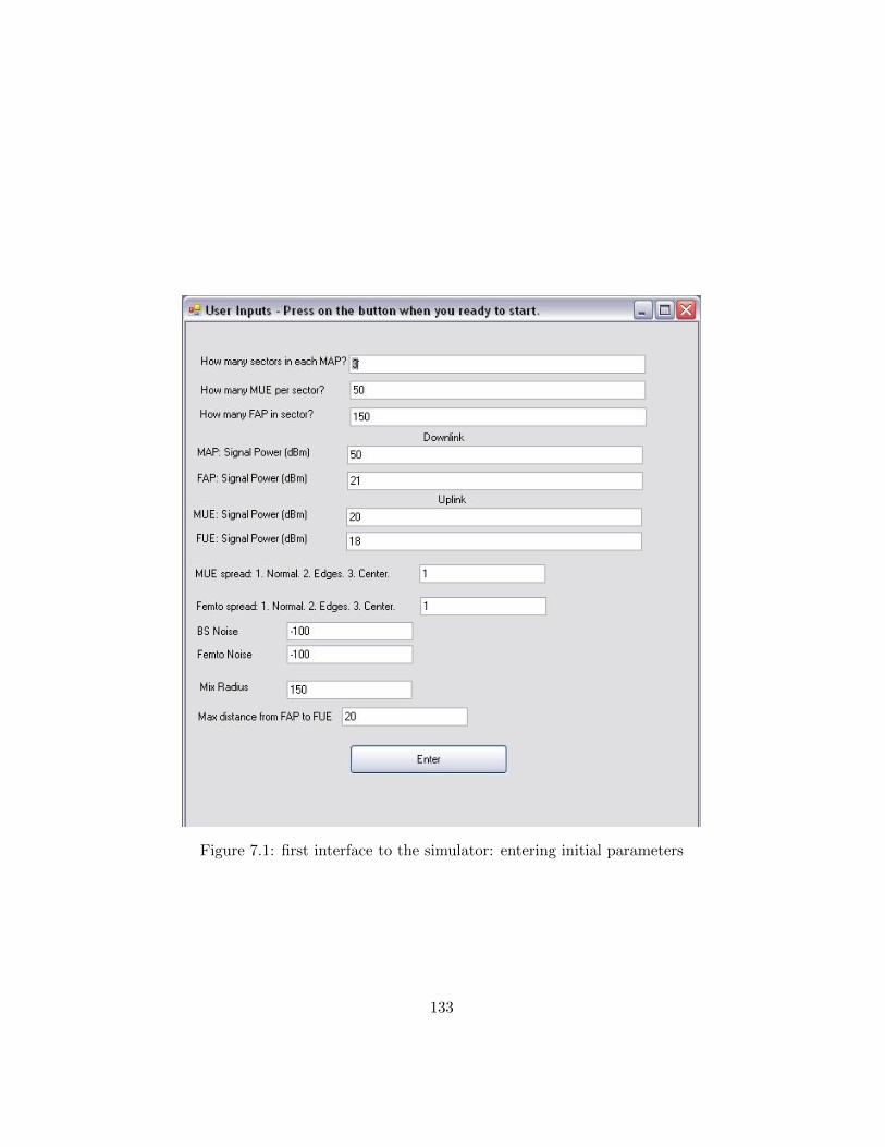
Figure 7.1: first interface to the simulator: entering initial parameters

133

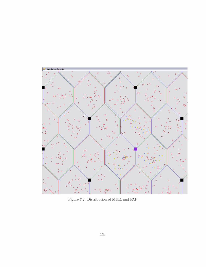
Figure 7.2: Distribution of MUE, and FAP

134

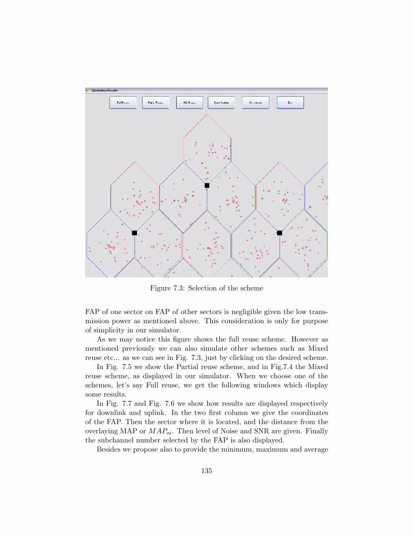
Figure 7.3: Selection of the scheme

FAP of one sector on FAP of other sectors is negligible given the low trans-mission power as mentioned above. This consideration is only for purposeof simplicity in our simulator.

As we may notice this figure shows the full reuse scheme. However asmentioned previously we can also simulate other schemes such as Mixedreuse etc... as we can see in Fig. 7.3, just by clicking on the desired scheme.

In Fig. 7.5 we show the Partial reuse scheme, and in Fig.7.4 the Mixedreuse scheme, as displayed in our simulator. When we choose one of theschemes, let’s say Full reuse, we get the following windows which displaysome results.

In Fig. 7.7 and Fig. 7.6 we show how results are displayed respectivelyfor downlink and uplink. In the two first column we give the coordinatesof the FAP. Then the sector where it is located, and the distance from theoverlaying MAP or MAPoi. Then level of Noise and SNR are given. Finallythe subchannel number selected by the FAP is also displayed.

Besides we propose also to provide the minimum, maximum and average

135

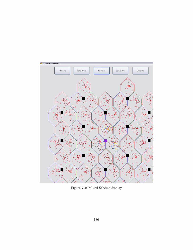
Figure 7.4: Mixed Scheme display

136

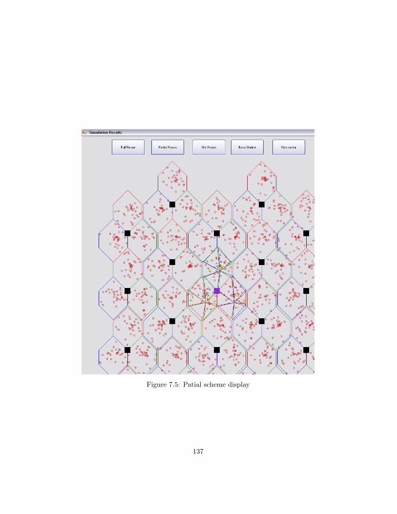
Figure 7.5: Patial scheme display

137

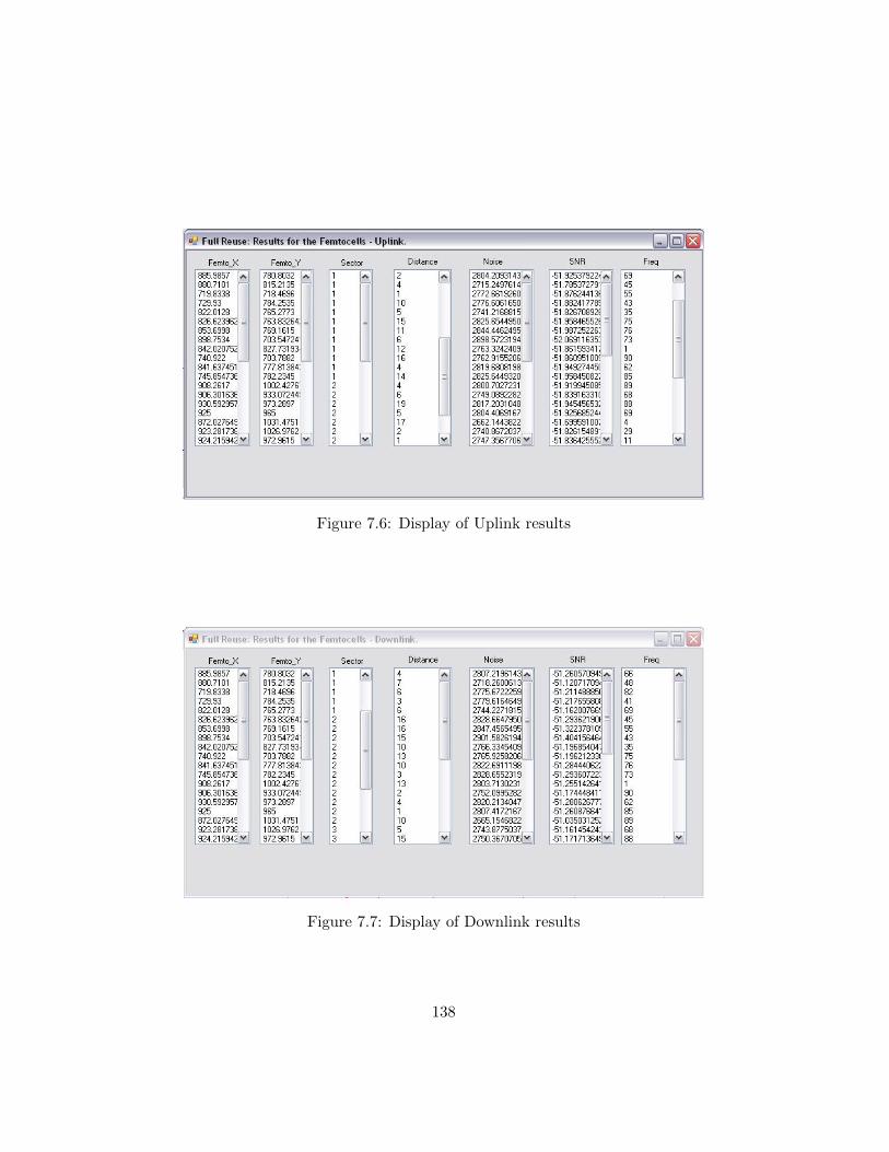
Figure 7.6: Display of Uplink results

Figure 7.7: Display of Downlink results

138

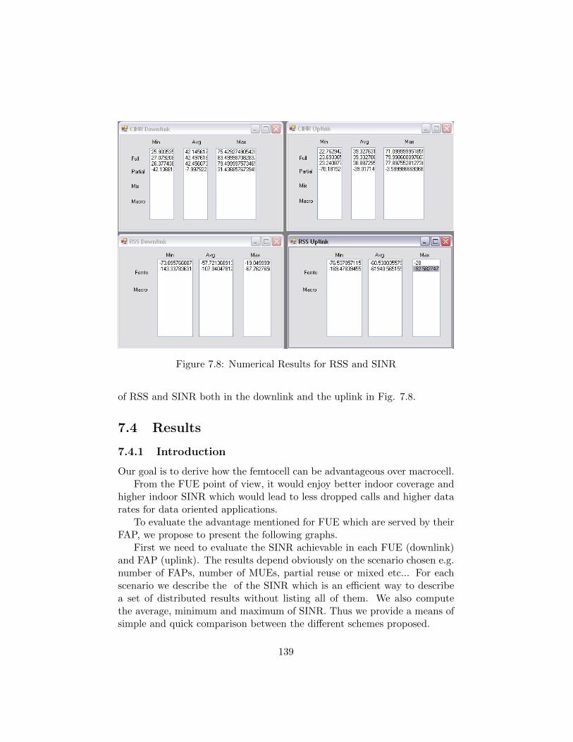
Figure 7.8: Numerical Results for RSS and SINR

of RSS and SINR both in the downlink and the uplink in Fig. 7.8.

7.4 Results

7.4.1 Introduction

Our goal is to derive how the femtocell can be advantageous over macrocell.From the FUE point of view, it would enjoy better indoor coverage and

higher indoor SINR which would lead to less dropped calls and higher datarates for data oriented applications.

To evaluate the advantage mentioned for FUE which are served by theirFAP, we propose to present the following graphs.

First we need to evaluate the SINR achievable in each FUE (downlink)and FAP (uplink). The results depend obviously on the scenario chosen e.g.number of FAPs, number of MUEs, partial reuse or mixed etc... For eachscenario we describe the of the SINR which is an efficient way to describea set of distributed results without listing all of them. We also computethe average, minimum and maximum of SINR. Thus we provide a means ofsimple and quick comparison between the different schemes proposed.

139

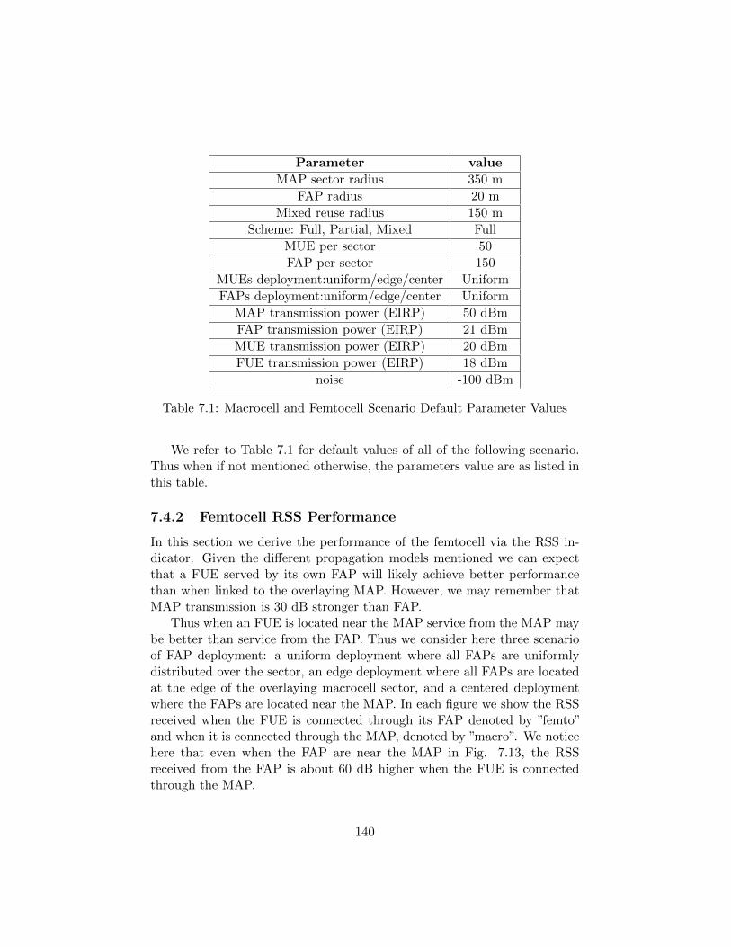
Parameter value

MAP sector radius 350 m

FAP radius 20 m

Mixed reuse radius 150 m

Scheme: Full, Partial, Mixed Full

MUE per sector 50

FAP per sector 150

MUEs deployment:uniform/edge/center Uniform

FAPs deployment:uniform/edge/center Uniform

MAP transmission power (EIRP) 50 dBm

FAP transmission power (EIRP) 21 dBm

MUE transmission power (EIRP) 20 dBm

FUE transmission power (EIRP) 18 dBm

noise -100 dBm

Table 7.1: Macrocell and Femtocell Scenario Default Parameter Values

We refer to Table 7.1 for default values of all of the following scenario.Thus when if not mentioned otherwise, the parameters value are as listed inthis table.

7.4.2 Femtocell RSS Performance

In this section we derive the performance of the femtocell via the RSS in-dicator. Given the different propagation models mentioned we can expectthat a FUE served by its own FAP will likely achieve better performancethan when linked to the overlaying MAP. However, we may remember thatMAP transmission is 30 dB stronger than FAP.

Thus when an FUE is located near the MAP service from the MAP maybe better than service from the FAP. Thus we consider here three scenarioof FAP deployment: a uniform deployment where all FAPs are uniformlydistributed over the sector, an edge deployment where all FAPs are locatedat the edge of the overlaying macrocell sector, and a centered deploymentwhere the FAPs are located near the MAP. In each figure we show the RSSreceived when the FUE is connected through its FAP denoted by ”femto”and when it is connected through the MAP, denoted by ”macro”. We noticehere that even when the FAP are near the MAP in Fig. 7.13, the RSSreceived from the FAP is about 60 dB higher when the FUE is connectedthrough the MAP.

140

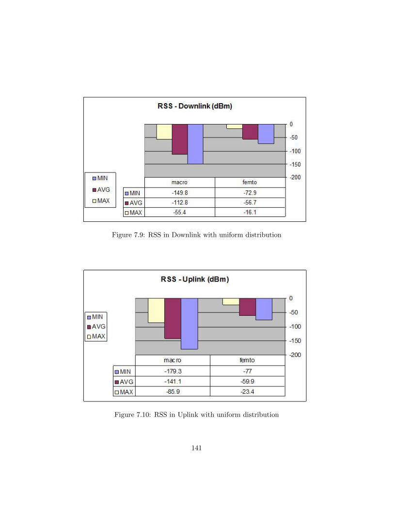
Figure 7.9: RSS in Downlink with uniform distribution

Figure 7.10: RSS in Uplink with uniform distribution

141

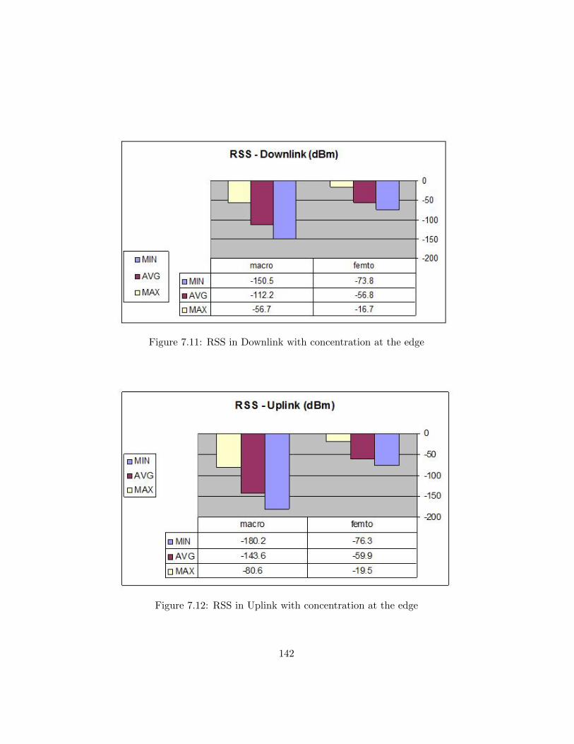
Figure 7.11: RSS in Downlink with concentration at the edge

Figure 7.12: RSS in Uplink with concentration at the edge

142

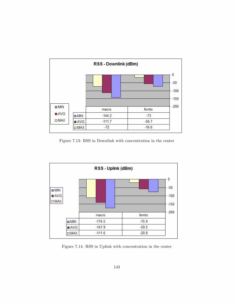
Figure 7.13: RSS in Downlink with concentration in the center

Figure 7.14: RSS in Uplink with concentration in the center

143

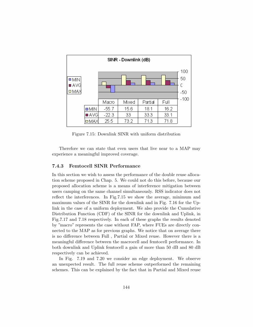
Figure 7.15: Downlink SINR with uniform distribution

Therefore we can state that even users that live near to a MAP mayexperience a meaningful improved coverage.

7.4.3 Femtocell SINR Performance

In this section we wish to assess the performance of the double reuse alloca-tion scheme proposed in Chap. 5. We could not do this before, because ourproposed allocation scheme is a means of interference mitigation betweenusers camping on the same channel simultaneously. RSS indicator does notreflect the interferences. In Fig.7.15 we show the average, minimum andmaximum values of the SINR for the downlink and in Fig. 7.16 for the Up-link in the case of a uniform deployment. We also provide the CumulativeDistribution Function (CDF) of the SINR for the downlink and Uplink, inFig.7.17 and 7.18 respectively. In each of these graphs the results denotedby ”macro” represents the case without FAP, where FUEs are directly con-nected to the MAP as for previous graphs. We notice that on average thereis no difference between Full , Partial or Mixed reuse. However there is ameaningful difference between the macrocell and femtocell performance. Inboth downlink and Uplink femtocell a gain of more than 50 dB and 80 dBrespectively can be achieved.

In Fig. 7.19 and 7.20 we consider an edge deployment. We observean unexpected result. The full reuse scheme outperformed the remainingschemes. This can be explained by the fact that in Partial and Mixed reuse

144

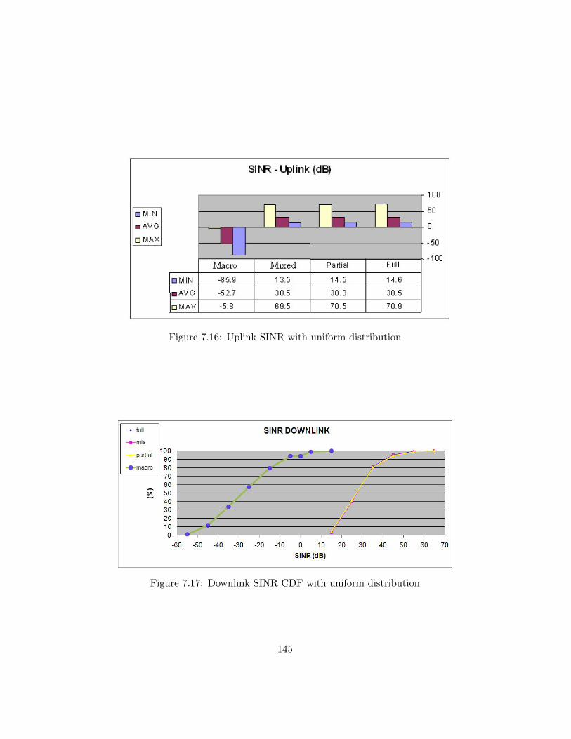
Figure 7.16: Uplink SINR with uniform distribution

Figure 7.17: Downlink SINR CDF with uniform distribution

145

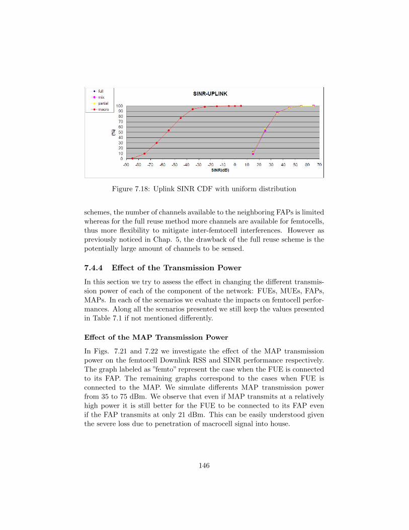
Figure 7.18: Uplink SINR CDF with uniform distribution

schemes, the number of channels available to the neighboring FAPs is limitedwhereas for the full reuse method more channels are available for femtocells,thus more flexibility to mitigate inter-femtocell interferences. However aspreviously noticed in Chap. 5, the drawback of the full reuse scheme is thepotentially large amount of channels to be sensed.

7.4.4 Effect of the Transmission Power

In this section we try to assess the effect in changing the different transmis-sion power of each of the component of the network: FUEs, MUEs, FAPs,MAPs. In each of the scenarios we evaluate the impacts on femtocell perfor-mances. Along all the scenarios presented we still keep the values presentedin Table 7.1 if not mentioned differently.

Effect of the MAP Transmission Power

In Figs. 7.21 and 7.22 we investigate the effect of the MAP transmissionpower on the femtocell Downlink RSS and SINR performance respectively.The graph labeled as ”femto” represent the case when the FUE is connectedto its FAP. The remaining graphs correspond to the cases when FUE isconnected to the MAP. We simulate differents MAP transmission powerfrom 35 to 75 dBm. We observe that even if MAP transmits at a relativelyhigh power it is still better for the FUE to be connected to its FAP evenif the FAP transmits at only 21 dBm. This can be easily understood giventhe severe loss due to penetration of macrocell signal into house.

146

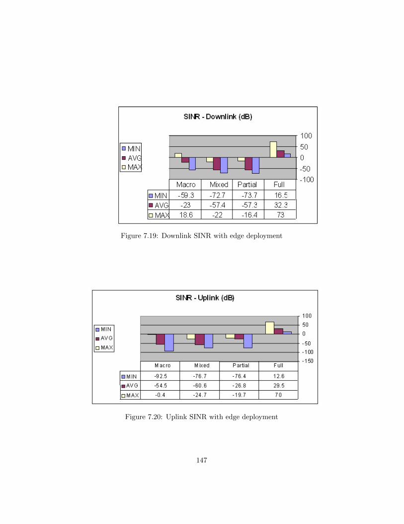
Figure 7.19: Downlink SINR with edge deployment

Figure 7.20: Uplink SINR with edge deployment

147

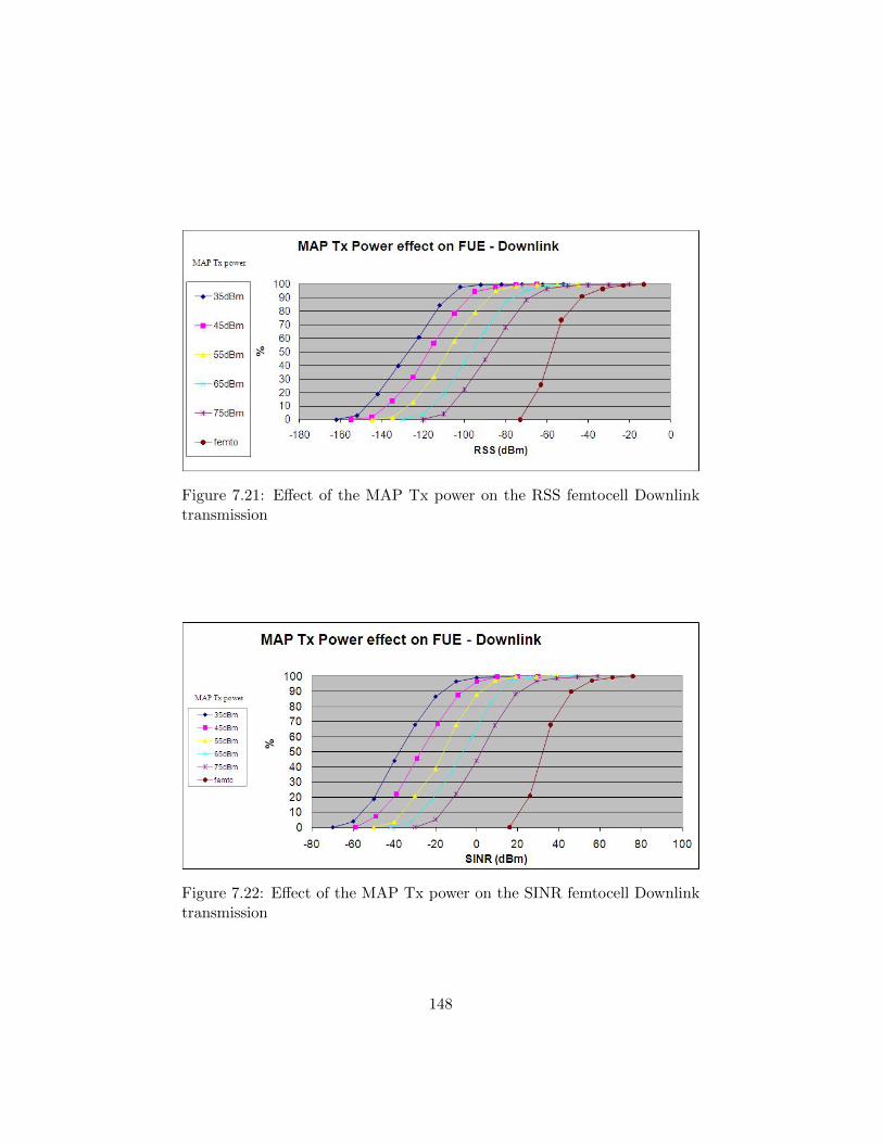
Figure 7.21: Effect of the MAP Tx power on the RSS femtocell Downlinktransmission

Figure 7.22: Effect of the MAP Tx power on the SINR femtocell Downlinktransmission

148

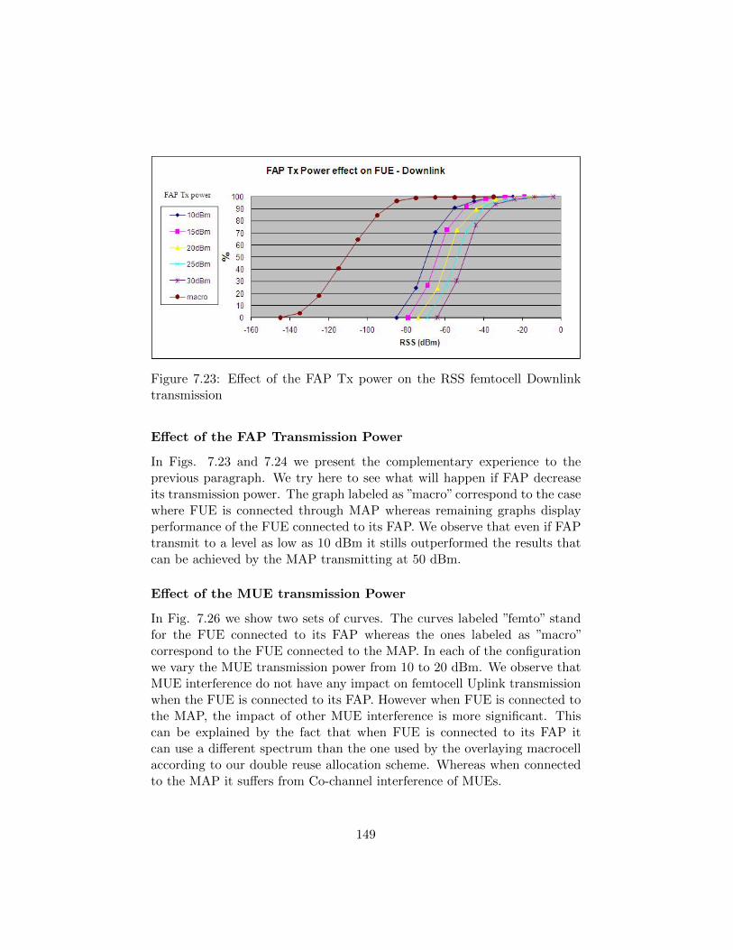
Figure 7.23: Effect of the FAP Tx power on the RSS femtocell Downlinktransmission

Effect of the FAP Transmission Power

In Figs. 7.23 and 7.24 we present the complementary experience to theprevious paragraph. We try here to see what will happen if FAP decreaseits transmission power. The graph labeled as ”macro” correspond to the casewhere FUE is connected through MAP whereas remaining graphs displayperformance of the FUE connected to its FAP. We observe that even if FAPtransmit to a level as low as 10 dBm it stills outperformed the results thatcan be achieved by the MAP transmitting at 50 dBm.

Effect of the MUE transmission Power

In Fig. 7.26 we show two sets of curves. The curves labeled ”femto” standfor the FUE connected to its FAP whereas the ones labeled as ”macro”correspond to the FUE connected to the MAP. In each of the configurationwe vary the MUE transmission power from 10 to 20 dBm. We observe thatMUE interference do not have any impact on femtocell Uplink transmissionwhen the FUE is connected to its FAP. However when FUE is connected tothe MAP, the impact of other MUE interference is more significant. Thiscan be explained by the fact that when FUE is connected to its FAP itcan use a different spectrum than the one used by the overlaying macrocellaccording to our double reuse allocation scheme. Whereas when connectedto the MAP it suffers from Co-channel interference of MUEs.

149

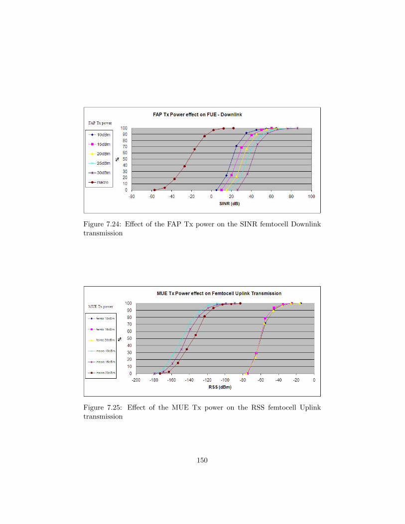
Figure 7.24: Effect of the FAP Tx power on the SINR femtocell Downlinktransmission

Figure 7.25: Effect of the MUE Tx power on the RSS femtocell Uplinktransmission

150

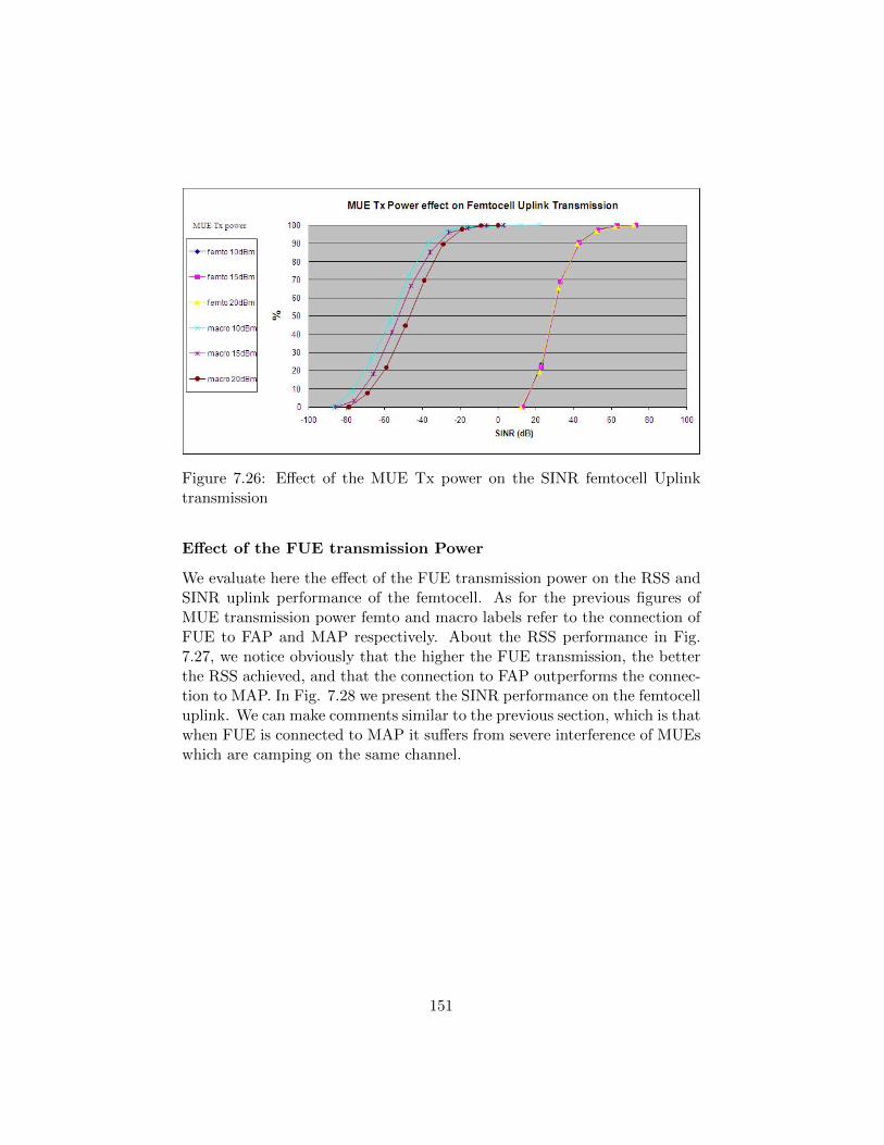
Figure 7.26: Effect of the MUE Tx power on the SINR femtocell Uplinktransmission

Effect of the FUE transmission Power

We evaluate here the effect of the FUE transmission power on the RSS andSINR uplink performance of the femtocell. As for the previous figures ofMUE transmission power femto and macro labels refer to the connection ofFUE to FAP and MAP respectively. About the RSS performance in Fig.7.27, we notice obviously that the higher the FUE transmission, the betterthe RSS achieved, and that the connection to FAP outperforms the connec-tion to MAP. In Fig. 7.28 we present the SINR performance on the femtocelluplink. We can make comments similar to the previous section, which is thatwhen FUE is connected to MAP it suffers from severe interference of MUEswhich are camping on the same channel.

151

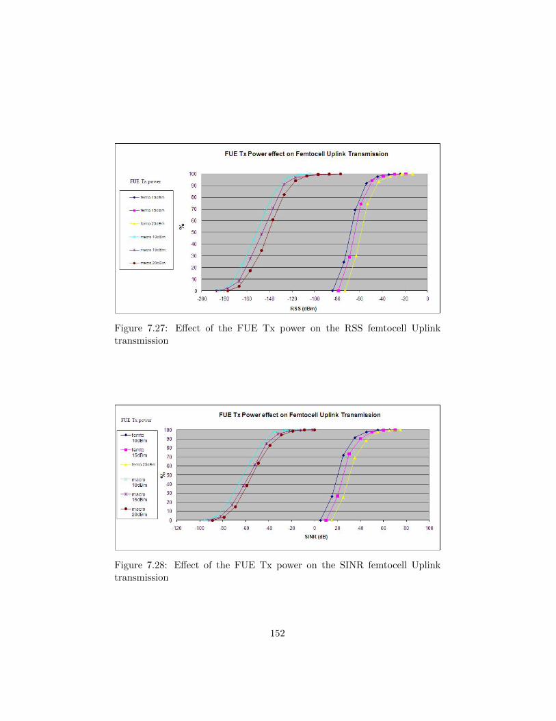
Figure 7.27: Effect of the FUE Tx power on the RSS femtocell Uplinktransmission

Figure 7.28: Effect of the FUE Tx power on the SINR femtocell Uplinktransmission

152

Chapter 8

Conclusion

After the unexpected success of 2G cellular networks to provide mobile userslocated outside their home with telephone services when moving outdoor,and the increasing deployment of cordless telephones when at home, weare currently experiencing an ever increasing demand for mobile broadbandinternet access when users are indoor. In this thesis we focused on twotechnologies: the WiFi technology, and the new femtocell technology. Thegoal of this thesis was to evaluate each of these two technologies separatelyfor the limiting factor to the capacity that can be offered to an end user.In the WiFi standard, the point that can be considered as the bottleneck ofthe performance is the multiple access mechanism to the radio resource byseveral users. In fact even if the CSMA/CA mechanism is a good tradeoffamong other access mechanisms such as TDMA, CDMA etc. because it isdistributed, to perform its task it still requires a set of waiting times whichleads to wasted resources. The challenge was to evaluate the performance ofthis mechanism, to be able to derive the usual performance indicator suchas throughput and delay. Due to the stochastic nature of this mechanism,theoretical models are always naturally used so as to describe the nature ofthe mechanism. Several models have already been developed but they areall based on simple assumptions. The most common assumptions are that ofan ideal channel, saturation throughput,etc. Besides this, existing accuratemodels do not deal with the enhanced MAC mechanism of the WiFi thatprovides QoS support.

In the first part of this thesis we developed an accurate EDCA modelbased on a four dimensional Markov chain. This model is an extension ofthe model of Kong et al. who extended the original Bianchi model. Wemodified this model to consider a non-ideal channel where errors occur with

153

a constant probability. We also consider different traffic scenarios: saturatedor unsaturated with different traffic loads. Thanks to our model we studiedthe effect of the different parameters of the EDCA mechanisms such asdifferentiation, or AIFS interframe space time, on the achievable throughput.We show that these parameters offer a good differentiation between accesscategories of different services. We also show the expected delay experiencedby a user given his AC. We see that the saturation factor q has a nonnegligible effect on the delay which confirms the importance of considering anon saturated model of the network. Thus our model is very rich, which onthe one hand makes it more accurate and closer to reality, but on the otherhand, requires more complex calculations. The main result of the modellies in the computation of the throughput which reflects the capacity of thesystem. This result is essential in order to design a deployment tool for WiFiQoS-enabled networks. Our non-saturated model avoid over dimensioningwhich would lead to interference between different access points.

In the second part of this thesis we assessed the performance of thefemtocell. We first presented the challenges and opportunities of this newtechnology. Then we focused on the main factor limiting performance whichis interference . This challenge is directly linked to the way we allocate theradio resources to this ”second tier” or second layer network. If we split thecommon spectrum shared between the macrocell and femtocell layers intotwo disjoint spectra we enjoy protection from co-channel interlayer interfer-ence. However spectrum efficiency is lost. On the other hand if we allow thetwo layers to share the spectrum we face severe interference . We presentedalready existing radio resource allocation schemes. We found an interestingfact: lots of methods have already been in existence for a long time and wereproposed at the time Femtocell was considered for the 2G GSM technolo-gies. However since the femtocell concept wasn’t seriously considered at thattime, the proposed allocation schemes were also somewhat ”forgotten”. Wepropose a novel allocation reuse scheme which allows mixing the two men-tioned approaches, namely spectrum splitting and spectrum sharing. Toincrease the efficiency of the network resource’s use, we proposed to reusethe channels belonging to the neighboring sector of the overlaying macrocell.Three different reuse plans have been proposed, each adapted to a specificscenario. We based our allocation scheme on the existing schemes we pre-sented before but that were proposed in the context of microcells or in otherdifferent technologies. Thus we apply these ideas to the concept of femtocell.We assumed that the underlying technology is OFDMA-based which allowsplitting the spectrum. Thus our scheme cannot be applied to 3G networksif the operator owns only a single band of frequencies. In the context of this

154

thesis we developed a static system level simulator which allows us to derivethe performance achievable by the femtocell when our allocation scheme isapplied. We present the RSS and SINR performance indicators achievedby femtocells for different scenarios. We show that femtocells outperformmacrocells in all configurations even when macrocells transmit at relativelyhigh power. In conclusion: can we answer the question ”which is the besttechnology?” Unfortunately we are still not able to name the winner. Firstof all there may be no winner. Because each technology offers a differentquality of service whether it is for data or voice service.

But to be able to consider the best technology even for a given servicewe have to deal with additional issues. For example we have to consideran end-to-end performance metric. Actually, both femtocell and WiFi arebackhauled by the fixed broadband connection of the user. But for thefemtocell, as soon as it has reached the gateway of the operator it is allocateddedicated resource in the core network whereas WiFi packet have to travelthrough regular path with all the congestions that can occur. So maybe WiFican offer higher data rates, especially if we consider the emerging 802.11 ”n”standard. But the required delay may not be suitable for delay sensitiveapplications such as VoIP based applications. Moreover some advantagescan be translated directly into physical performance metrics. For example,one of the main advantages of femtocells is that it allows the use of the samehandset already bought, whereas a dual-mode handset is required if we wishour mobile phone to get connected to the WiFi network. Therefore anextended study which includes some financial parameters is required. It willhave to compute the CapEx(Capital Expenditure) and OpEx (OperationalExpenditure) savings from both the operator’s and users’ point of view. Inaddition to the just mentioned open issue we propose as future work thefollowing research orientation. WiFi CSMA/CA access mechanism allowsnatural interference mitigation. As soon as an undergoing transmission isdetected, all other stations are prevented from initiating new transmissions.This is true even for stations that are associated to an adjacent AP (i.e. notthe one which is transmitting or receiving at that time). Thus given thatthere is a limited number of non-overlapping channels used by WiFi deviceswe have to extend our model to a scenario with multiple cells and not onlya single cell. In this manner we could account for additional throughputdecreases.

For the femtocell, we considered here a rather simple channel selectionbased on the least noisy channel. Therefore this can be considered as agreedy algorithm. It would be interesting to assess the performance of thefemtocell when a more optimal scheme is used for the sharing of the fre-

155

quency between femtocells. Game theory may be helpful to this issue.

156

Chapter 9

Appendix :Fixed PointTheorem Method

We use here a famous theorem often useful for numerical problems:

Theoreme 1 Let X ⊂ Rn, n ≥ 1 a closed set, and ‖ · ‖ a norm on R. LetF : X → X be a function such that there is α ∈ [0, 1[ such that

‖F (x)− F (y)‖ ≤ α‖x− y‖

for all x, y ∈ X. Thus there is a single point P ∈ X such that F (P ) = P .Moreover, let x0 ∈ X and let (xk)k∈N the sequence defined by induction byxk+1 = F (xk) for k ∈ N. Therefore limk→+∞ xk = P and we have

‖xk − P‖ ≤ αk‖x0 − P‖ (CV )

for all k ∈ N.

Remark: A priori, one does not know P , But thanks to the inequality(CV ), we get a very good approximation because the convergence is very,very fast(α < 1!!): the dream for a computer scientist. That’s why we tryas soon as possible to reduce to a fixed point problem .

Step 1: nomenclature.. We denote ~τ = (τ0, ..., τ3) et ~b = (b0, ..., b3),where for simplicity b0, ..., b3 denote the vector coordinates of b0,0,0,0. Wedenote

p(~τ)i = (1− pe)pi + pe

= (1− pe)(1− (1−Π3j=0(1− τj)Π3

j=i+1(1− τj)) + pe

157

We have the relationship

τi = (1 + p(~τ)i + ...+ (p(~τ)i)m+h)bi

for all i, and thus,

bi =τi

1 + p(~τ)i + ...+ (p(~τ)i)m+h.

Then we define the function f : R4 → R4 with its coordinates:

(f(~τ))i =τi

1 + p(~τ)i + ...+ (p(~τ)i)m+h,

and, for ~b fixed, we try to solve f(~τ) = ~b, i.e.

F (~τ) = ~τ ,

withF (~τ) = ~τ − f(~τ) +~b.

It was reduced to a fixed point theorem problem: we will try now to applythe theoreme. Let fixed first of all a ”pleasant” norm:

‖x‖ = sup{|xi|/ i = 0, 1, 2, 3, 4}.

Step 2: Shrinking. Let ~τ , ~τ ′ ∈ [0, 1]4. Let i ∈ {0, 1, 2, 3}. We have

|(F (~τ)− F (~τ ′))i|

=

∣∣∣∣−(~τ − ~τ ′)i(

1− 1

1 + p(~τ)i + ...+ (p(~τ)i)m+h

)−(~τ ′)i

(1

1 + p(~τ)i + ...+ (p(~τ)i)m+h− 1

1 + p(~τ ′)i + ...+ (p(~τ ′)i)m+h

)∣∣∣∣≤(

1− 1

m+ h+ 1

)‖~τ − ~τ ′‖+ ‖~τ ′‖

∑m+hk=1 (p(~τ)i)

k − (p(~τ ′)i)k(∑m+h

k=0 (p(~τ)i)k)(∑m+h

k=0 (p(~τ ′)i)k)(9.1)

The problem is to evaluate the second term of the right side. We put A =p(~τ)i and B = p(~τ ′)i. With a small calculation we get:

m+h∑k=1

Ak −Bk =

m+h∑k=1

(A−B)

k−1∑j=0

AjBk−1−j

= (A−B)

m+h−1∑j=0

m+h−1∑k=j

AjBk−j

= (A−B)

m+h−1∑j=0

Ajm+h−1−j∑

k=0

Bk

158

Because A,B > 0, we get∣∣∣∣∣m+h∑k=1

Ak −Bk

∣∣∣∣∣ ≤ |A−B| ·m+h−1∑

j=0

Aj

·m+h−1∑

j=0

Bj

and thus∣∣∣∑m+h

k=1 Ak −Bk∣∣∣(∑m+h

j=0 Aj)·(∑m+h

j=0 Bj) ≤ |A−B| ·(1− Am+h∑m+h

j=0 Aj

)·

(1− Bm+h∑m+h

j=0 Bj

)

Because A = p(~τ)i ∈ [pe, 1] and also for B, by taking formula (9.1), we get

|(F (~τ)− F (~τ ′))i| ≤(

1− 1

m+ h+ 1

)‖~τ − ~τ ′‖+ |p(~τ)i − p(~τ ′)i|

(1− pm+h

e

m+ h+ 1

)2

(9.2)

It remains therefore to evaluate p(~τ)i − p(~τ ′)i. We write it: p(~τ)i = (1 −pe)Π

3j=0(1− τj)Mj , with Mj ∈ {M − 1,M}. For k ∈ {0, .., 3}, we have

∂p(~τ)i∂τk

= −(1− pe) · (1− τk)Mk−1Πj 6=k(1− τj)Mj .

We assume henceforth that M ≥ 2. Then we get∣∣∣∣∂p(~τ)i∂τk

∣∣∣∣ ≤ (1− pe)M

Thus for ~τ , ~τ ′, there is t0 ∈]0, 1[ such that

|p(~τ)i − p(~τ ′)i| =

∣∣∣∣∣4∑

k=0

∂pi∂τk

(t~τ + (1− t)~τ ′) · (τk − τ ′k)

∣∣∣∣∣≤ 4(1− pe)M‖~τ − ~τ ′‖ (9.3)

If we substitute (9.3) into (9.2), we get

|F (~τ)− F (~τ ′)| ≤ α‖~τ − ~τ ′‖

with

α = 1− 1

m+ h+ 1+ 4(1− pe)M

(1− pm+h

e

m+ h+ 1

)2

. (9.4)

159

Thus,if we manage to get pe close to 1 (i.e. a big probabilty of error in apacket !), then we have α < 1.

remark: The problem is that in the formula of α, if M is big, we are in aproblem... We can maybe refine: Let be δ ∈ [0, 1] and let us consider thedomain

Dδ = {~τ ∈ [0, 1]4/∃j tel que 1− τ j ≤ δ}

Then we get that ∣∣∣∣∂p(~τ)i∂τk

∣∣∣∣ ≤ (1− pe)MδM−2

for all ~τ ∈ Dδ. In this case, if δ < 1, we have limM→+∞MδM−2 = 0, andwe get back a small coefficient in the formula of α.

Step 3: F is defined on [0, 1]4, and it has to get its value in [0, 1]4 too. Letbe i ∈ {0, ..., 3}. With the same caculation as in step 2, we get

|F (τ)i| ≤(

1− 1

m+ h+ 1

)‖~τ‖+ ‖~b‖

Thus if we set that

‖~b‖ ≤ 1

m+ h+ 1,

we have |F (~τ)i| ≤ 1. The concern is that F (~τ)i is not always positive...Thus we set

F (~τ) = (max{0, F (~τ)0}, ...,max{0, F (~τ)3})

And now all go well: F : [0, 1]4 → [0, 1]4 and ‖F (~τ) − F (~τ ′)‖ ≤ α‖~τ − ~τ ′‖.Finally the theorem states that there is ~τ such that F (~τ) = ~τ .

Let us show that F (~τ) = ~τ . Let be i. We have F (~τ)i = τi.

Case 1: if τi > 0, then F (~τ)i > 0, and therefore F (~τ)i = F (~τ)i.

Case 2: if τi = 0, we have F (~τ)i = 0, and thus F (~τ)i ≤ 0. But becauseτi = 0, we have F (~τ)i = bi ≥ 0, thus F (~τ)i = F (~τ)i = 0.

In brief, in all cases, F (~τ) = F (~τ) = ~τ , and thus f(~τ) = ~b, and we find asolution that converges fast. To summarize we have the following Theorem:

Theoreme 2 Assume that ‖~b‖ ≤ 1m+h+1 . Assume that α < 1, where α is

given by (9.4). Then there is ~τ ∈ [0, 1]4 such that f(~τ) = ~b, and we can geta very good approximation of ~τ .

160

Bibliography

[1] IEEE STD 802.11-1999, IEEE Standard for Information technology-Telecommunications and information exchange between systems-Localand metropolitan area networks-Specific requirements - Part 11: Wire-less LAN Medium Access Control (MAC) and Physical Layer (PHY)Specifications, 1999.

[2] Digital cellular telecommunications system (phase 2+); gsm cordlesstelephony system (cts), phase 1; service description; cts radio interfacelayer 3 specification. Draft GSM 04.56 version 8.0.0 Release 1999, Mars200.

[3] Feasibility study for enhanced uplink for utra fdd (release 6). 3GPPTechnical Report TR 25.896 V6.0.0 (2004-03), 3GPP, Mar. 2004.

[4] Wireless Medium Access Control (MAC) and Physical Layer (PHY)Specifications: Medium Access Control (MAC) Quality of Service En-hancements, IEEE Std. 802.11e, Sep 2005.

[5] Ieee standard for local and metropolitan area networks part 16: Air in-terface for fixed and mobile broadband wireless access systems amend-ment 2: Physical and medium access control layers for combined fixedand mobile operation in licensed bands and corrigendum 1. IEEE Std802.16e-2005 and IEEE Std 802.16-2004/Cor 1-2005 (Amendment andCorrigendum to IEEE Std 802.16-2004), pages 1–822, 2006.

[6] IEEE Std. 802.11-2007, IEEE Standard for Information technology-Telecommunications and information exchange between systems-Localand metropolitan area networks-Specific requirements - Part 11: Wire-less LAN Medium Access Control (MAC) and Physical Layer (PHY)Specifications(Revision of IEEE Std 802.11-1999), June 2007.

[7] Interference management in umts femtocells. Technical report, FemtoForum, Dec. 2008.

161

[8] 3GPP. Hnb and hnb-macro propagation models. TSG-RAN WG4 44-bis R4-071617, Qualcomm Europe, Oct 2007.

[9] Norman Abramson. The aloha system: another alternative for com-puter communications. In AFIPS ’70 (Fall): Proceedings of the Novem-ber 17-19, 1970, fall joint computer conference, pages 281–285, NewYork, NY, USA, 1970. ACM.

[10] F. Alizadeh-Shabdiz and S. Subramanian. A finite load analytical modelfor the ieee 802.11 distributed coordination function mac. In Proceed-ings of the Workshop on Modeling and Optimization in Mobile, Ad Hocand Wireless Networks (WiOpt ’03), page 321U322, Sophia Antipolis,France, March 2003.

[11] M. Almgren, L. Bergstrom, M. Frodigh, and K. Wallstedt. Channel al-location and power settings in a cellular system with macro and microcells using the same frequency spectrum. In Vehicular Technology Con-ference, 1996. ’Mobile Technology for the Human Race’., IEEE 46th,volume 2, pages 1150 –1154, April 1996.

[12] Jeffrey G. Andrews, Arunabha Ghosh, and Rias Muhamed. Funda-mentals of WiMAX: Understanding Broadband Wireless Networking.Prentice Hall, Sep. 2007.

[13] A. Banchs and L. Vollero. A delay model for 802.11e edca. IEEECommunications Letters, 9(6):508–510, June 2005.

[14] L. Berlemann, S. Mangold, G. Hiertz, and B. Walke. Delay performanceof the enhanced distributed channel access of ieee 802.11e. In ISTMobile Summit 06, page 5, Mykonos, Greece, Jun 2006.

[15] G. Bianchi. IEEE 802.11-Saturation throughput analysis. IEEE Com-munications Letters, 2:318–320, 1998.

[16] G. Bianchi. Performance Analysis of the IEEE 802.11 Distributed Coor-dination Function. IEEE Journal on Selected Areas in Communications,18(3):535–547, 2000.

[17] G. Bianchi, L. Fratta, and M. Oliveri. Performance Evaluation andEnhancement of the CSMA/CA protocol for 802.11 Wireless LAN. InProc. PIMRC, pages 392–396, Oct. 1996.

162

[18] F. Cali, M. Conti, and E. Gregori. IEEE 802.11 wireless LAN: Capacityanalysis and protocol enhancement. In IEEE INFOCOM, volume 1,pages 142–149, Mars 1998.

[19] Frederico Calı, Marco Conti, and Enrico Gregori. Dynamic tuningof the ieee 802.11 protocol to achieve a theoretical throughput limit.IEEE/ACM Trans. Netw., 8(6):785–799, 2000.

[20] G. R. Cantieni, N. Qiang, C. Barakat, and T. Turletti. Performanceanalysis under finite load and improvements for multirate 802.11. Com-puter Communications, 28(10):1095–1109, June 2005.

[21] Vikram Chandrasekhar and Jeffrey G. Andrews. Uplink capacity andinterference avoidance for two-tier cellular networks. In GLOBECOM,pages 3322–3326. IEEE, 2007.

[22] P. Chatzimisios, V. Vitsas, and A. C. Boucovalas. Throughput anddelay analysis of the ieee 802.11 protocol. In proc of IEEE internationalWorkshop on Networked Appliances (IWNA), pages 168–174, 2002.

[23] S.T.S. Chia. Radio and network resource management for third gener-ation mobile systems. In Vehicular Technology Conference, 1993 IEEE43rd, pages 935 –937, 18-20 1993.

[24] I Chih-Lin, L.J. Greenstein, and R.D. Gitlin. A microcell/macrocellcellular architecture for low- and high-mobility wireless users. SelectedAreas in Communications, IEEE Journal on, 11(6):885 –891, Aug 1993.

[25] Dong-Hoon Cho, Jung-Hoon Song, Min-Su Kim, and Ki-Jun Han. Per-formance analysis of the ieee 802.16 wireless metropolitan area network.volume 0, pages 130–137, Los Alamitos, CA, USA, 2005. IEEE Com-puter Society.

[26] H. Claussen. Performance of macro- and co-channel femtocells in ahierarchical cell structure. In Personal, Indoor and Mobile Radio Com-munications, 2007. PIMRC 2007. IEEE 18th International Symposiumon, pages 1–5, 2007.

[27] Jurgen Deissner, Andre Noll Barreto, Ulrich Barth, and Gerhard Fet-tweis. Interference analysis of a total frequency hopping gsm cordlesstelephony system. In GSM Cordless Telephony System,T Proc. PIM-RCS98, pages 1525–1529, 1998.

163

[28] Jurgen Deissner and Gerhard Fettweis. Increased capacity through hi-erarchical cellular structures with inter-layer reuse in an enhanced gsmradio network. Mobile Networks and Applications, 6(5):471–480, 2001.

[29] X.J. Dong and P. Varaiya. Saturation throughput analysis of IEEE802.11 Wireless LANs for a lossy channel. IEEE Communications Let-ters, 9(2):100–102, 2005.

[30] Paal Engelstad and Olav N. Østerbø. Delay and throughput analysis ofieee 802.11e edca with starvation prediction. In LCN, pages 647–655.IEEE Computer Society, 2005.

[31] H. Eriksson, B. Gudmundson, J. Skold, J.K. Ugland, and P. Willars.Multiple access options for cellular based personal communications. InVehicular Technology Conference, 1993 IEEE 43rd, pages 957 –962,18-20 1993.

[32] Chuan Heng Foh and Juki Wirawan Tantra. Comments on ieee 802.11saturation throughput analysis with freezing of backoff counters. IEEECommun. Lett, 9:130–132, 2005.

[33] M. Frullone, G. Riva, P. Grazioso, and C. Carciofi. Analysis of optimumresource management strategies in layered cellular structures. In Uni-versal Personal Communications, 1994. Record., 1994 Third AnnualInternational Conference on, pages 371 –375, 27 1994.

[34] M. Frullone, G. Riva, P. Grazioso, and G. Falciasecca. Advanced plan-ning criteria for cellular systems. Personal Communications, IEEE,3(6):10 –15, dec 1996.

[35] H. Furukawa and Y. Akaiwa. A microcell overlaid with umbrella cellsystem. In Vehicular Technology Conference, 1994 IEEE 44th, pages1455 –1459 vol.3, 8-10 1994.

[36] R.W. Gibson, R.J.G. MacNamee, and S.K. Vadgama. Universal mobiletelecommunication system - a concept. Telecommunications, 21(11):23,Nov 1987.

[37] David Gonzalez, Virginia Corvino, Silvia Ruiz, Joan Olmos, MarioGarcia-Lozano, and Roberto Verdone. Downlink resource allo-cation in lte:centralized vs. distributed approach. In Proc. ofCOST2100/NEWCOM++ WPR.8 Workshop on Radio Resource Al-location for LTE, Wien, Austria, Sep. 2009.

164

[38] Association GSM. Mobile world celebrates four billion connections gsmworld. Webpage, Feb. 2009.

[39] I. Guvenc, M. Jeong, F. Watanabe, and H. Inamura. A hybrid frequencyassignment for femtocells and coverage area analysis for co-channel op-eration. IEEE Commun. Lett., 12(12), Dec 2008.

[40] Armin Heindl and Reinhard German. Performance modeling of ie802.11 wireless lans with stochastic petri nets. Performance Evalua-tion, 44:139–164, 2001.

[41] L.T.W. Ho and H. Claussen. Effects of user-deployed, co-channel femto-cells on the call drop probability in a residential scenario. In Personal,Indoor and Mobile Radio Communications, 2007. PIMRC 2007. IEEE18th International Symposium on, pages 1 –5, 3-7 2007.

[42] Jie Hui and Michael Devetsikiotis. A unified model for the performanceanalysis of ieee 802.11e edca. IEEE Transactions on Communications,53(9):1498–1510, Spetember 2005.

[43] International Telecommunication Union (ITU). Mobile overtakes fixed.Webpage, Feb 2003.

[44] H.-S. Jo, J.-G. Yook, C. Mun, and J. Moon. A self-organized up-link power control for cross-tier interference management in femtocellnetworks. In Proc. IEEE Military Communications Conference (MIL-COM), San Diego, CA, Nov. 2008.

[45] Y. Kinoshita and M.A. Henriques. High density space division multipleaccess: Double reuse of frequency channels. In Proc. of InternationalConference on Universal Personal Communications, pages 552 – 557,San Diego, CA, Sept 1994.

[46] Y. Kinoshita, T. Tsuchiya, and S. Ohnuki. Frequency common use be-tween indoor and cellular radio U research on frequency channel doublyreused cellular system. In Proc. of the 39th IEEE Vehicular TechnologyConference (VTC’89), volume 1, pages 329 – 335, San Francisco, CA,May 1989.

[47] Yasuaki Kinoshita and David K. Asano. Frequency double reuse for in-door and urban digital cellular telephone systems U enhanced concep-tual design formulae for single handset systems. In Proc. of the Multiac-cess, Mobility and Teletraffic for Personal Communications Workshop(MMT S97), pages 247–257, 1997.

165

[48] Z. Kong, D.H.K. Tsang, B. Bensaou, and D. Gao. Performance analysisof IEEE 802.11e contention-based channel access. IEEE Journal onSelected Areas in Communications, 22(10):2095–2106, December 2004.

[49] Y.-L. Kuo, E. H.-K. Lu, C.-H.and Wu, G.-H. Chen, and Y.-H. Tseng.Performance analysis of the enhanced distributed coordination functionin the ieee 802.11e. In in Proc. IEEE Vehicular Technology Conference- VTC ’03 - Fall, pages 3488–3492. Oct, 2003.

[50] X. Lagrange. Multitier cell design. Communications Magazine, IEEE,35(8):60 –64, aug 1997.

[51] Long Le and E. Hossain. Multihop cellular networks: Potential gains,research challenges, and a resource allocation framework. Communica-tions Magazine, IEEE, 45(9):66 –73, sep. 2007.

[52] Haipeng Lei, Xin Zhang, and Dacheng Yang. A novel frequency reusescheme for multi-cell ofdma systems. In Vehicular Technology Con-ference, 2007. VTC-2007 Fall. 2007 IEEE 66th, pages 347 –351, sept.2007.

[53] D. Lopez-Perez, A. Valcarce, G. De La Roche, Enjie Liu, and Jie Zhang.Access methods to wimax femtocells: A downlink system-level casestudy. pages 1657 –1662, nov. 2008.

[54] David Lopez-Perez, Akos Ladanyi, Alpar Juttner, and Jie Zhang.OFDMA femtocells: A self-organizing approach for frequency assign-ment. In PIMRC (Personal, Indoor and Mobile Radio Communica-tions), Tokyo, Japan, sep 2009. IEEE.

[55] S. Mangold, G. HIERTZ, and B WALKE. Ieee 802.11e wireless lan- resource sharing with contention based medium access. In proc. ofIEEE Personal Indoor Mobile Radio Conference (PIMRC), Beijing P.R. China, Sept 2003.

[56] Qiang Ni, Lamia Romdhani, Thierry Turletti, and Imad Aad. Qos issuesand enhancements for ieee 802.11 wireless lan. Rapport de recherche4612, INRIA, Sophia Antipolis, November 2002.

[57] J. W. Robinson and T. S. Randhawa. Saturation throughput analysisof IEEE 802.11e Enhanced Distributed Coordination Function. IEEEJournal on Selected Areas in Communications, 22(5):917–928, 2004.

166

[58] M. Salem, A. Adinoyi, H. Yanikomeroglu, and D. Falconer. Opportu-nities and challenges in ofdma-based cellular relay networks: A radioresource management perspective. Vehicular Technology, IEEE Trans-actions on, Feb 2010.

[59] C. Shannon. The zero-error capacity of a noisy channel. IRE Transac-tions on Information Theory, 1956.

[60] C. E. Shannon. Communication in the Presence of Noise. Proceedingsof the IRE, 37(1):10–21, 1949.

[61] M. I. Silventoinen, M. Kuusela, and P. A. Ranta. Analysis of a newchannel access method for home base station. In Proc.of 5th IEEE Inter-national Conference on Universal Personal Communications (ICUPC),pages 930–935, Cambridge, MA, USA, 1996.

[62] Marko I. Silventoinen. GSM Evolution Towards 3rd Generation Sys-tems, chapter In-door Base Station Systems : Improving GSM to meetlow-tier challenge, pages 235–261. Springer US, 2002.

[63] K. Stamatiou and J.G. Proakis. A performance analysis of codedfrequency-hopped ofdma [cellular system]. In Wireless Communica-tions and Networking Conference, 2005 IEEE, volume 2, pages 1132 –1137 Vol. 2, 13-17 2005.

[64] Y. C. Tay and K. C. Chua. A capacity analysis for the ieee 802.11 macprotocol. Wirel. Netw., 7(2):159–171, 2001.

[65] Fouad A. Tobagi. Distributions of packet delay and interdeparture timein slotted aloha and carrier sense multiple access. J. ACM, 29(4):907–927, 1982.

[66] Alvaro Valcarce, David Lopez-Perez, Guillaume De La Roche, and JieZhang. Limited access to ofdma femtocells. In Proc. of IEEE Personal,Indoor and Mobile Radio Communications Symposium (PIMRC), 2009.

[67] Haifeng Wang and J. Lilleberg. Conventional and scrambling ofdmsystem switch in multicell environments. In Wireless Communicationsand Networking Conference, 2006. WCNC 2006. IEEE, volume 1, pages1 –5, 3-6 2006.

[68] Li-Chun Wang, G.L. Stuber, and Chin-Tau Lea. Architecture design,frequency planning, and performance analysis for a microcell/macrocell

167

overlaying system. Vehicular Technology, IEEE Transactions on,46(4):836 –848, nov 1997.

[69] J. Weitzen and T. Grosch. Comparing coverage quality for femtocelland macrocell broadband data services. Communications Magazine,IEEE, 48(1):40 –44, jan. 2010.

[70] Krzysztof Wesolowski. Introduction to Digital Communication Systems.Wiley, 2009.

[71] P.D. White, M.K. Gurcan, and R.J.G. MacNamee. 900 mhz digitalcordless telephone. In IEE Proceedings-F: Communications,Radar andsignal proceedings, volume 132, pages 425–432. Philips, Research Lab-oratories, Redhill, UK, August 1985.

[72] J Yin, X Wang, and D P Agrawal. Optimal packet size in error-pronechannel for ieee 802.11 distributed coordination function. In Proc. IEEEWCNC’04, pages 1654–1659, Atlanta, USA, March 2004.

[73] J Yin, X Wang, and D P Agrawal. Modeling and optimization of wire-less local area network. Computer Communications, 28(10):1204–1213,June 2005.

[74] J. Zhang and G. de la Roche. Femtocells Technologies and Deployment.Wiley, 2010.

[75] Eustathia Ziouva and Theodore Antonakopoulos. CSMA/CA perfor-mance under high traffic conditions: throughput and delay analysis.Computer Communications, 25(3):313–321, 2002.

168

Publications

Y. Haddad, D. Porrat. Femtocell SINR Performance Evaluation.InProc. of International Conferences on Access Networks, Services and Tech-nologies. IARIA ACCESS 2010. Valencia Spain, September 2010.

Y. Haddad, D. Porrat. A Two-Tier Frequency Reuse Scheme inProc. Of Second International Workshop on Indoor and Outdoor Femtocells (IOFC’10) in conjunction with IEEE PIMRC’10, Turkey, September2010.

Y. Haddad, D. Porrat. Femtocell: Opportunities and Challengesof the Home Cellular Base Station for the 3G . In Proc. of IADISInternational Multi Conference on Computer Science and Information Sys-tems (session on Wireless Applications and Computing), Algarve, Portugal,June 2009.

Y. Haddad, G. Le Grand. Throughput analysis of the IEEE 802.11eEDCA on a noisy channel in unsaturated mode in Proc. of the 3rdACM International Workshop on Wireless Multimedia Networking and Per-formance Modeling (WMuNeP) October 2007.

Y. Haddad, G. Le Grand. Performance Analysis of IEEE 802.11eEDCA under Finite Load in an Error Prone Channel. In Proc. ofJDIR’2007, France, January 2007.

169