An Access Delay Model for IEEE 802.11e EDCA

1

An Access Delay Model for IEEE 802.11e EDCADongxia Xu,Student Member, IEEE, Taka Sakurai,Member, IEEE,and Hai L. Vu,Senior Member, IEEE

Abstract— In this paper, we analyse the MAC access delayof the IEEE 802.11e EDCA mechanism under saturation. Wedevelop a detailed analytical model to evaluate the influenceof all EDCA differentiation parameters, namely AIFS, CWmin,CWmax and TXOP limit, as well as the backoff multiplier β.We derive explicit expressions for the mean, standard deviationand generating function of the access delay distribution. Byapplying numerical inversion on the generating function, we areable to efficiently compute values of the distribution. Throughcomparison with simulation, we confirm the accuracy of ouranalytical model over a wide range of operating conditions. Usingthe model, we derive simple asymptotics and approximations forthe mean and standard deviation of the access delay, which revealthe salient model parameters for performance under differentdifferentiation mechanisms. We also use the model to study thecharacteristics of CWmin, AIFS, TXOP, and β differentiation.We find that, though rejected during the standardization process,β differentiation is an effective differentiation mechanism thathas some advantages over the other mechanisms.

Index Terms— Medium access delay, IEEE 802.11e, QoS,EDCA, service differentiation, generating function.

I. INTRODUCTION

A quality of service (QoS) extension to the original IEEE802.11 wireless local area network standard [1], known

as IEEE 802.11e [2], defines a contention-based mediumaccess control (MAC) scheme calledenhanced distributedchannel access(EDCA). EDCA provides service differenti-ation by separating flows into different access classes. Thedifferentiation achieved by EDCA is relatively easy to under-stand in a qualitative sense; however, quantifying the degreeof differentiation provided is difficult due to the distributed,contention-based nature of EDCA. Hence, there is a need foraccurate performance models to guide the configuration ofparameters. In this paper, we develop a detailed analyticalmodel of the packet access delay in a network of 802.11eEDCA stations operating under saturation. In this context,access delay is the time interval between the instant a packetreaches the head of the transmission queue, and the time whenthe packet is successfully received at the destination station.

Service differentiation in EDCA is effected through fourparameterized access categories (ACs). Packets belongingtodifferent ACs are given different access priorities by appro-priate tuning of four AC-specific parameters. The parametersdefine, respectively, the size of AC-dependent guard peri-ods (arbitrary interframe spacing orAIFS), minimum and

D. Xu is with the National ICT Australia (NICTA), Victoria Laboratory,Department of Electrical and Electronic Engineering, The University ofMelbourne, VIC 3010, Australia.

T. Sakurai is with the Department of Electrical and Electronic Engineering,The University of Melbourne, VIC 3010, Australia.

H. L. Vu is with the Centre for Advanced Internet Architectures, Faculty ofI.C.T., Swinburne Univ. of Technology, P.O. Box 218, VIC 3122, Australia.

maximum contention windows (CWmin and CWmax), andlengths of packet bursts or transmission opportunity limit(TXOP limit). A fifth parameter representing the backoffwindow multiplier (sometimes called the persistence factor),which we denote byβ, was studied during the standardizationprocess, but was eventually abandoned due to doubts abouteffectiveness [3] and replaced with a fixed multiplier of 2. Inthe present paper, we substantially extend a model [4] thatwe developed previously for access delay in the distributedcoordination function (DCF) of the original IEEE 802.11MAC, to EDCA. Our model can scale to an arbitrary numberof ACs and accounts for all four standardized differentiationparameters. We also make our model general enough to coverβ differentiation, so that we can study the characteristics ofthis mechanism. Note that parts of this work have appearedpreviously in conference form [5], [6].

Many recent papers have proposed analytical models forvarious subsets of EDCA functionality [7]-[19]. Xiao [7]modelsCWmin andCWmax differentiation, [8]-[18] modelCWmin, CWmax and AIFS differentiation, and Peng et.al. [19] develop a simple model forTXOP differentiationonly. Compared to previous models, our model is novel forthe following reasons: (i) it correctly accounts for all 4differentiation parameters in the standard; (ii) it yieldsthestandard deviation and distributional values of the accessdelay,as well as the commonly obtained mean access delay; (iii) andit provides accurate estimates of these metrics. Ge at al. [20]attemp to explicitly account for all differentiation parametersin their model, but they actually analyse and simulate ap-persistent version of EDCA, which does not have the samecharacteristics as EDCA. In [14], it is stated that a 4-parametermodel can be built by simply inflating the packet length intheir 3-parameter model to account forTXOP differentiation.However, as we will show in our model development, an accu-rate model ofTXOP differentiation is a non-trivial extensionthat requires careful consideration of all possible combinationsof transmission and collision durations of the different ACs,together with their probabilities of occurrence.

Our analytical model is a fully integrated one that cancapture joint differentiation by up to four parameters (or fiveparameters includingβ). However, for ease of understanding,we present the model in terms of three sub-models: a collisionprobability model that estimates the collision probabilitiesof the different classes; a delay model that accounts for allphenomena that contribute to the access delay; and aTXOPmodel that accounts forTXOP differentiation. The collisionprobability and delay models capture the influence of theCWmin, CWmax and AIFS mechanisms. By virtue of theway in which theTXOP mechanism operates, it becomesnatural to treat it as a modelling extension.

A collision probability model is a vital element of any

2

EDCA analysis. All the aforementioned studies use ex-tensions of Bianchi’s two-dimensional (2-D) Markov chainanalysis of DCF [21] to derive the collision probabilities,though [12] shows that there are other approaches. To in-corporateAIFS differentiation, [8]-[10] resort to 3-D Markovchains, while [11] uses a 4-D Markov chain. In contrast, [16]and [17] develop less complex models based on separate 2-and 1-D Markov chains. Our collision probability model isbased on that of [16], but uses an average value analysis inplace of the 2-D Markov chain. This leads to a more intuitiveand simple, yet accurate collision probability model.

Our delay andTXOP models are novel and yield de-tailed statistics of the access delay. Most prior studies ofEDCA analyse only throughput and/or mean delay. Exceptionsare [10], where the delay distribution is obtained using acomputational approach based on the transient analysis ofa Markov chain; [18], where the delay distribution is ap-proximated by estimating the probabilities of alternate delayoutcomes; and Engelstad and Østerbø [15], where points of thedistribution are obtained by inverting the generating functionof the delay distribution. In our study, we present a moredirect and accurate method to obtain the delay distribution.Similar to [15], we derive the generating function of thedistribution of the access delay and obtain distributionalvaluesvia numerical transform inversion. However, our generatingfunction is more detailed and accurate than that of [15], as weillustrate through a numerical comparison. Further, we obtainexplicit expressions for the mean and standard deviation ofthe access delay. Our moment expressions are derived viadirect probabilistic arguments and not by differentiationandlimit-taking of the generating function, which is the approachused in [15]. The direct approach is advantageous becausethe generating function in question is complicated, makingdifferentiation tedious. Perhaps as a result of this complexity,Engelstad and Østerbø [15] go no further than state thestandard deviation in terms of derivatives of the generatingfunction. As far as we are aware, ours is the first work to obtainan explicit expression for the standard deviation of the delay(or jitter) in EDCA. The expression enables use to developanalytical insights into the relative importance of parametersand to quantify the jitter performance of the differentiationmechanisms.

Achieving accuracy in the distributional values clearly de-mands a more detailed analysis than one that is sufficient fordelivering accuracy in throughput or mean delay. In our delaymodel, we carefully account for all events that noticeablycontribute to the access delay of a packet from a taggedstation. We include the delays due to the backoff process ofthe tagged station, interruptions to the countdown of theAIFSguard-time by higher priority stations, collisions involvingthe tagged station, and transmissions and collisions involvingother stations. We develop the delay andTXOP models interms of random variables, which makes it possible to readilyobtain explicit expressions for the mean, standard deviation,and generating function. We confirm that our analytical resultsfor the mean, standard deviation and distribution of the accessdelay are accurate through comparison with ns-2 simulation.Significantly, we have found that our analytical tail distribution

is typically an excellent match with simulation down to10−3,and often beyond.

In addition to developing an analytical model, we exploit themodel to advance the understanding of EDCA delay perfor-mance. We use the model to deriveasymptoticsfor the meanunder the assumptions of unlimited retransmissions and thenumber of contending stations tending to infinity, and to deriveapproximations for both the mean and standard deviationunder the assumptions of a finite retransmission limit anda large number of contending stations. The asymptotics andapproximations reveal the salient model parameters for perfor-mance under different differentiation mechanisms, and providesimpler alternatives to the complete analytical expressions forsystem analysis and design. Our approximation methodologyand results are new. Our asymptotic work is inspired by that ofRamaiyan et al. [22], who obtained asymptotics for throughputratios underCWmin, AIFS andβ only differentiation. Thereare some parallels between their asymptotic throughput ratiosand our asymptotic mean delay ratios (since under infinite re-transmissions, the mean access delay has a simple relationshipwith the throughput). Unlike [22], we also derive asymptoticresults for the individual ACs rather than the ratios, as well asa result forTXOP differentiation.

Finally, we perform a detailed numerical study using theanalytical model to quantify the differentiation in the mean andstandard deviation afforded byCWmin, AIFS, TXOP andβ. We find thatβ differentiation, though discarded during thestandardization process, is an effective differentiationmecha-nism that has some advantages over the other mechanisms.We also find thatCWmin and AIFS individually provideonly coarse-grained differentiation, but that jointCWmin andAIFS can provide access to intermediate differentiation levels.

The rest of this paper is organized as follows. In Section II,we give a summary of the EDCA mechanism. As EDCA hasbeen thoroughly reviewed in many previous papers (e.g. [23]),we keep our description brief. In Section III, we present ouranalytical model for the MAC access delay, starting with thecollision probability model. Then we describe our access delaymodel that takes into account theCWmin, CWmax, AIFSandβ mechanisms, and derive expressions for the associatedmean, standard deviation and generating function. At the endof this section, we present ourTXOP model, and derive themean, standard deviation and generating function when allfive differentiation parameters are included. In Section IV,we present asymptotics and approximations for the mean andstandard deviation. The validation of the analytical modelwithns-2 simulation is carried out in Section V, and then we use themodel to assess the nature of the service separation providedby each differentiation mechanism, and to test the accuracyof the approximations. Finally, we state our conclusions inSection VI.

II. OVERVIEW OF EDCA

EDCA is a prioritized carrier sense multiple access withcollision avoidance (CSMA/CA) access mechanism whichuses (truncated) binary exponential backoff (BEB). It realizesservice differentiation through the use of four ACs in each

3

station. Each AC has its own transmission queue and four ad-justable contention parameters:CWmin, CWmax, AIFS andTXOP limit. When a packet arrives at the MAC layer fromthe higher layers, it is assigned to one of the ACs according toits user priority. The parameter values of different ACs shoulddiffer in at least one parameter to enable differentiation.

The CWmin and CWmax parameters define the initialand maximum values of the contention window (CW) usedin the backoff process. In this process, a discrete backofftime measured in backoff slots is randomly selected from[0,CW-1]. A backoff entity is maintained by each AC in thestation. The backoff timer counts down as long as the channelis idle but is frozen when the channel is busy. When thebackoff timer reaches zero, the station starts transmitting. Ifthe transmission is successful, the receiving MAC layer sendsan ACK (acknowledgement) after a short interframe spacingtime, SIFS. Upon failure to receive anACK (indicating anerrored transmission or collision), theCWs of the sendersare doubled, and the packets are scheduled for retransmission.Doubling of CW continues in response to further collisionsuntil CWmax is reached, after which CW is maintained atCWmax until the packet is successfully transmitted, or untilthe maximum permitted number of attempts is reached.

The AIFS parameter defines the guard time that a stationmust observe after a busy channel period before its backofftimer can be resumed. A smallerAIFS means a higherpriority of access. The value ofAIFS is always greater thanSIFS to ensure contention-free access for ACKs and othercontrol packets. If anAIFS countdown is interrupted by atransmission from a higher priority station, the countdownis stopped and a newAIFS countdown is started when thechannel becomes idle.

TheTXOP limit parameter defines the maximum durationfor which a station can enjoy uninterrupted control of themedium after obtaining a transmission opportunity. Uninter-rupted control is guaranteed by allowing the station to sendits next data packet after aSIFS time following the receipt ofan ACK for the previous packet. A value ofTXOP limit = 0indicates only a single packet may be transmitted for eachtransmission opportunity.

Like DCF, EDCA can operate in either two-way (DATA-ACK) or four-way (RTS-CTS-DATA-ACK) handshakingmodes. In our analysis, we cover the two-way handshakingmode only, but the analysis can be readily extended to thefour-way mode.

III. ANALYTICAL MODEL

In our model, we make the following assumptions:(i) allstations are saturated (always have a packet to send);(ii) thecollision probability is constant regardless of the state,butmay differ with AC; (iii) channel conditions are ideal;(iv)ACK packets are transmitted at the lowest basic rate andthe ACK timeout after a collision matches the guard timeobserved by non-colliding nodes, and (v) each station onlyhas traffic belonging to a single AC. The firstfour assumptionsare standard for studies of 802.11 performance and originatefrom [21]. Assumptions (iv) and (v)can be removed at theexpense of additional modelling complexity.

We allow for an arbitraryJ distinct ACs in the network.Without loss of generality, we label the ACs with indicesk = 1, . . . , J , in order of non-decreasingAIFS, while plac-ing no ordering restrictions on the values of the other ACparameters. We refer to thekth AC as AC[k], and denotethe associatedAIFS period byAIFSk. The number of AC[k]stations is denoted bynk, R is the maximum number ofattempts (the same for all ACs as specified in [2]), andWk

is the minimum contention window for AC[k]. We generalizethe backoff mechanism in this paper to exponential backoffwith real multiplier βk > 1, instead of binary exponentialbackoff as in the standard. The maximum backoff stage forAC[k] is mk, so that the maximum contention window isCWmaxk = 〈βmk

k Wk〉, where 〈.〉 denotes rounding to thenearest integer. The transmission opportunity limit for AC[k]is denoted byTXOPk.

A. Collision Probability Model

Our objective is to develop a fixed-point approximation tocompute the collision probabilities and transmission probabili-ties of all the ACs. Letck andpk denote the collision probabil-ity and transmission probability, respectively, experienced byan AC[k] packet. The fixed-point approximation is establishedby combining a set of equations for the collision probabilitiesexpressed in terms of the transmission probabilities, withanopposing set of equations for the transmission probabilitiesexpressed in terms of the collision probabilities. We obtain theformer set of equations by following an approach proposed byKim and Kim [16], which we summarize below.

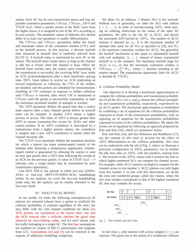
Kim and Kim [16], and also Robinson and Randhawa [17],use the concept ofslot class to account for the effect ofAIFS differentiation on the collision probability. Slot classcan be understood with the aid of Fig. 1, where we illustrate aparticular configuration ofAIFSk parameters. Let us numberthe idle slots after anAIFS1 with slot numbers, starting from1. The increase in theAIFSk values withk restricts the slots inwhich higher-numbered ACs can compete for channel access.For example, while AC[1] stations can begin to compete for thechannel access in slot number 1, AC[2] stations can only beginfrom slot number 2. In line with this observation, we dividethe slots into numbered groups called slot classes, where theslot class number corresponds to that of the highest numberedAC that may compete for access.

Fig. 1. Slot Number and Slot Class

In slot classj, only stations with access categoryk ≤ j cantransmit. This gives rise to the notion of a conditional collision

4

probability ck(j) for AC[k] in slot classj, given by

ck(j) = 1 −

∏ji=1 rni

i

rk, (k ≤ j), (1)

where we defineri = 1 − pi.The overall collision probabilityck is obtained as an average

of the ck(j)’s weighted by the stationary probabilitiesP (j)that a randomly selected slot belongs to slot classj:

ck =J∑

j=k

ck(j)P (j)

∑Ji=k P (i)

. (2)

The probabilitiesP (j) can be found by examining theevolution of the slot number/class. In [16], it is shown thatthe evolution can be described by a Markov chain. Each stateof the Markov chain represents a slot number, and a transitionis made at each slot according to whether the slot is idle ormarks the beginning of a successful transmission or collision.If the slot is idle, the slot number is increased by one; if itis not idle, the slot number is reset to 1. The probabilitiesP (j) can be computed from the steady state probabilities ofthe Markov chain as

P (j) =Q(j)

∑Ji=1 Q(i)

, (3)

Q(j) =1 − αh(j+1)−h(j)

j

1 − αj

j−1∏

i=1

αh(i+1)−h(i)

i ,

where we define∏0

i=1 αh(i+1)−h(i)

i = 1, and

αj =

j∏

k=1

rnk

k , h(j) =AIFSj − AIFS1

tslot.

Equations (1), (2) and (3) expressck as a non-linear functionof the transmission probabilitiespk. To find pk as a functionof the collision probabilitiesck, [16] and [17] use variants ofthe 2-D Markov chain of [21]. In contrast, we invoke a mean-value approximation forpk by equating it to the reciprocalof the average backoff periodof an AC[k] station. In otherwords, if Ψk is the average backoff period, then we write

pk =1

Ψk. (4)

To find the average backoff period, we analyse the dynamicsof the backoff process in a similar way to Kwak et al. [24],who analysed the backoff process for DCF. The evolution ofthe backoff process of an AC[k] station at transmission instantscan be described by a discrete-time Markov chains(t) withnon-zero transition probabilities

P (s(t + 1) = i|s(t) = i − 1) = ck, i = 1, . . . , R − 1,

P (s(t + 1) = 0|s(t) = i) = 1 − ck, i = 0, . . . , R − 2,

P (s(t + 1) = 0|s(t) = R − 1) = 1, i = R − 1.

It is straightforward to show that the steady-state probabilitiesof s(t) are given byπ(k)

i = (1 − ck)cik(1 − cR

k )−1, for i =0, . . . , R − 1.

Let U(k)i be a discrete uniform random variable (r.v.)

representing the backoff duration that an AC[k] station has

to wait in the ith backoff stage. These r.v.’s have densitiesdefined by

P [U(k)i = j] =

{u(0, 〈βi

kWk〉 − 1) for i = 0, ...,mk − 1,

u(0, 〈βmk

k Wk〉 − 1) for i = mk, ..., R − 1,

(5)

where u(a, b) is the discrete uniform density with sup-port (a, . . . , b). The corresponding average backoff durations,E[U

(k)i ], are given by

E[U(k)i ] =

{〈βi

kWk〉−12 for i = 0, ...,mk − 1,

〈βmkk

Wk〉−1

2 for i = mk, ..., R − 1.(6)

Knowing the steady state probabilities and average durationsof the R backoff stages, it follows that the overall averagebackoff period of an AC[k] station is

Ψk =

R−1∑

i=0

π(k)i E[U

(k)i ]

=

mk−1∑

i=0

ηkcki(〈βk

iWk〉 − 1

2)

+R−1∑

i=mk

ηkcki(〈βk

mkWk〉 − 1

2), (7)

whereηk = (1 − ck)(1 − cRk )−1.

Equations (1), (2), (3), (4) and (7) constitute a non-linearsystem of equations that can be solved iteratively to obtainthepk’s andck ’s.

B. Delay Model

We consider a selected (tagged) AC[k] station and derivean expression for the access delay as experienced by packetsof this station under saturation conditions. From the protocoldescription in Section II, we can identify several events thatcontribute to the access delay. The most obvious is simplythe successful transmission of the packet. Preceding this eventwill be the first backoff plus a variable number of collisionsinvolving the tagged station and the associated backoff peri-ods. Successful transmissions and collisions not involving thetagged station also contribute to the access delay, since theymanifest as interrupts to the backoff counter.

The access delayD(k) of the tagged station can be writtenas

D(k) = ǫ(k) + A(k) + T (k), (8)

whereǫ(k) is a r.v. representing a defer period, which includesthe duration ofAIFSk and the interruptions to this durationfrom higher priority stations;A(k) is a r.v. representing thesum of the durations of backoffs and collisions involving thetagged station, as well as the durations of successful transmis-sions and collisions of non-tagged stations that interruptthebackoff timer of the tagged station. The last term,T (k), is thetransmission time of the packet by the tagged station.

As mentioned previously, we first focus on the case ofTXOPi = 0 (i = 1, . . . , J), which means only one packettransmission is permitted per channel access. In the case of

5

fixed length data packets, this means thatT (k) = tdata, wheretdata denotes the transmission time of a single data packet.Later in Section III-E, we will remove this restriction onTXOPi.

The defer periodǫ(k) accounts for the duration ofAIFSk,as well as any interruptions toAIFSk by transmissions fromhigher priority stations, namely AC[j] stations wherej < k.Since AIFSj < AIFSk, an AC[j] station has the right toaccess the channel before the channel has been idle forAIFSk.In this event, the tagged station resets theAIFSk timer andstarts a new countdown once the channel becomes idle again.Therefore, any number of interruptions by AC[j] stations arepossible beforeAIFSk can be successfully counted down.

We now obtain an expression forǫ(k). Clearly,ǫ(1) = AIFS1

since there is no interruption to the highest priority stations.On the other hand, the defer period for AC[k] stations withk > 1 must account for interruptions by any higher prioritystations in any of theh(k) slots. As in Section III-A, we referto the successive idle slots followingAIFS1 as slots1 to h(k).We denoteϕ(i) as the slot class to which sloti belongs. Theprobability that at least one higher priority station transmits inslot 1 is

µ1 = 1 −

ϕ(1)∏

i=1

rni

i . (9)

The excess time due to an interruption in slot 1 from thepoint of view of the tagged station is

t1 = AIFS1 + X1. (10)

The r.v. Xi represents the duration of the interruption inslot i; it could be a successful transmission when only onetransmission occurs, or a collision when more than one stationattempts to transmit.

If there is no transmission in slot1, the probability that atleast one higher priority station transmits in slot2 is

µ2 =

ϕ(1)∏

i=1

rni

i (1 −

ϕ(2)∏

j=1

rnj

j ), (11)

and the excess time for the tagged station is

t2 = AIFS1 + tslot + X2. (12)

This argument can be continued for allh(k) slots; the respec-tive quantities for sloth(k) are

µh(k) = [h(k)−1∏

i=1

ϕ(i)∏

j=1

rnj

j ][1 −

ϕ(h(k))∏

l=1

rnl

l ],

th(k) = AIFS1 + (h(k) − 1)tslot + Xh(k) . (13)

The duration of interruptionsXi (i = 1, . . . , h(k)) can beexpressed as

Xi =

{T ∗ w.p. ρ(i)C∗ w.p. 1 − ρ(i),

(14)

where w.p. stands for ‘with probability’;T ∗ is the channeloccupancy of a successful transmission from a higher prioritystation;C∗ is the channel occupancy of a collision involvinghigher priority stations. The quantityρ(i) is the probability

of a successful transmission,conditional on at least onetransmission. In the case when all data packets in the systemare uniform and have fixed length, we have1

T ∗ = C∗ = tdata + SIFS + tack,

and

ρ(i) =

∑ϕ(i)l=1 nlplr

nl−1l

∏ϕ(i)j=1j 6=l

rnj

j

1 −∏ϕ(i)

l=1 rnl

l

. (15)

The numerator in (15) is the probability ofexactly onetransmission, while the denominator is the probability ofatleast one transmission.

The defer periodǫ(k) can be interpreted as the waiting timeuntil the first success in a sequence of independent trials,where each trial hash(k)+1 possible outcomes correspondingto theh(k) types of interrupts plus the successful countdown ofAIFSk. The probability of a successful countdown ofAIFSk

is

s(k) = 1 −h(k)∑

j=1

µj =h(k)∏

i=1

ϕ(i)∏

j=1

rnj

j . (16)

Putting everything together, we have

ǫ(k) = i1t1 + i2t2 + . . . + ih(k)th(k) + AIFSk

w.p.(∑h(k)

l=1 il)!∏h(k)

l=1 il!µi1

1 µi22 · · ·µ

ih(k)

h(k) s(k), (17)

wherei1, i2, . . . , ih(k) = 0, 1, . . .∞ are non-negative integers.The integersi1, i2, . . . , ih(k) represent the number of inter-ruptions to each type of slot, and they extend to infinitysince any number of interruptions is possible. The differentinterruption types can occur in any order, which is capturedby the multinomialcoefficient inthe probability mass function(pmf) in (17).It can be confirmed that the probabilities in (17)sum to one through an application of the multinomial theorem.

Next we address the second term in (8),A(k). Since thenumber of backoff intervals that the tagged station experi-ences depends on the number of retransmissions, the value ofA(k) strongly depends on the number of retransmissions. Thenumber of retransmissions before success takes a truncatedgeometric distribution with pmfηkci

k for i = 0, ..., R− 1. Wecan therefore write

A(k) = A(k)i w.p. ηkci

k, (18)

wherei = 0, ..., R−1. The r.v.A(k)i is comprised ofi collisions

involving the tagged station,i + 1 backoff intervals and theinterruptions to them. It can be expressed as

A(k)i =

i∑

j=0

B(k)i,j +

i∑

j=1

C(k)i,j , (19)

whereB(k)i,j represents the backoff intervals and the interrup-

tions, andC(k)i,j represents the channel occupancy of a collision

1holds true forC∗ due to the first part of assumption (iv), and becauseEIFS − DIFS = SIFS + tack (see [1]).

6

involving the tagged station. The r.v.’sC(k)i,j are all i.i.d. and

B(k)i,j are i.i.d. in the indexi.For uniform and fixed packet lengths, we have

C(k) = tdata + SIFS + tack + ǫ(k), (20)

where thei, j subscripts are suppressed for notational clarity.The scope ofB(k)

i,j is defined by a backoff interval thattakes a discrete uniform distribution. In EDCA, each slot ofthe backoff interval can be interrupted at most once withcertain probabilities, either by a successful transmission froma non-tagged station, or by a collision involving the non-tagged stations. Each interruption causes the backoff timerto be frozen, and after the channel becomes idle again, thebackoff process resumes from the next slot. Based on this, forany i, we can expressBj as a random sum

B(k)j =

U(k)j∑

n=1

Y (k)n , (22)

whereY(k)n is i.i.d. and represents the interruption to thenth

backoff slot, andU (k)j is the backoff interval given by (5).

In the following, we suppress the indexn from Y(k)n for

clarity. If no other station transmits,Y (k) is equal to theduration of a slot timetslot. If there is only one transmission, itis equal to the channel occupancy of a successful transmission,denoted asG(k). When more than one non-tagged stationattempts to transmit,Y (k) equals the channel occupancy ofa collision involving non-tagged stations, denoted byH(k).Hence we obtain

Y (k) =

tslot w.p. 1 − ck

G(k) w.p. γ(k)

H(k) w.p. ν(k),(23)

where γ(k) and ν(k) are the corresponding probabilities forsuccessful transmissions and collisions, respectively.Like ck,γ(k) and ν(k) must be determined by averaging over thedifferent slot classes:

γ(k) =

J∑

j=k

γ(k)(j)P (j)

∑Ji=k P (i)

,

whereγ(k)(j) can be obtained as (21).The first term in (21)is the probability that exactly one of the non-tagged AC[k]stations transmits and no other station transmits; the secondterm is the sum of the probabilities that exactly one of theAC[i] (i 6= k) stations transmits and no other station transmits.Given γ(k), ν(k) can be computed fromν(k) = ck − γ(k). Inthe case of uniform, fixed length packets, we have

G(k) = H(k) = tdata + SIFS + tack + ǫ(k). (24)

C. Generating Function

Now we derive the generating function of the distributionof the access delay for the caseTXOPi = 0 (i = 1, . . . , J),using the analysis of the previous section. We use the following

notational convention for a generating function: ifX is a non-negative, integer-valued random variable, then the generatingfunction of the pmf ofX is

X(z) =∑∞

r=0 P (X = r)zr for z ∈ C.

All the r.v.’s introduced in III-B are non-negative, but notal-ways integer-valued. However, they can be easily transformedto integer-valued r.v’s by defining a lattice with spacingδ, suchthat the values of all r.v.’s are concentrated on the latticepoints,and then scalingδ to 1. In the sequel, we abuse the notationslightly by reusing the r.v. names that appear in Section III-B torefer to their integer-valued equivalents. For example, wewriteP (D(k) = r), r = 0, 1, . . . for the pmf of the integer-valuedaccess delayD(k), andD(k)(z) for the generating function.

We can immediately obtain an expression forD(k)(z) from(8):

D(k)(z) = A(k)(z)T (k)(z)ǫ(k)(z). (25)

In the following, we suppress the superscript(k) from thegenerating functions for notational clarity. For the case of fixedlength packets, we have

T (z) = ztdata/δ. (26)

Based on (18), we can findA(z) as:

A(z) =

R−1∑

i=0

ηkcikAi(z). (27)

From (19), we obtain

Ai(z) = C(z)i

i∏

j=0

Bj(z). (28)

It follows from (20) that

C(z) = ǫ(z)zω, (29)

whereω is an integer constant defined byω = (tdata+SIFS+tack)/δ.

From (22), the generating function ofB(k)j is given by

Bj(z) = Uj(Y (z)). (30)

Equation (5) yields

Uj(z) =

{1−zf(j)

f(j)(1−z) for j = 0, ...,mk − 1,1−zf(mk)

f(mk)(1−z) for j = mk, ..., R − 1,

wheref(j) = 〈βjkWk〉.

From (23) it follows that

Y (z) = (1 − ck)ztslot/δ + γG(z) + νH(z), (31)

where it is easy to obtain from (24) that

G(z) = H(z) = ǫ(z)zω. (32)

The next step is to find the generating function ofǫ(k). Forthe highest priority class, AC[1], we have that

ǫ(z) = zAIFS1/δ. (33)

7

γ(k)(j) = (nk − 1)pkrnk−2k

j∏

i=1i6=k

rni

i + rnk−1k

j∑

i=1i6=k

[nipirni−1i

j∏

l=1l 6=k,l 6=i

rnl

l ]. (21)

E[Y (k)] = (1 − ck)tslot + γ(k) E[G(k)] + ν(k) E[H(k)], (34)

V[Y (k)] = (1 − ck)(tslot − E[Y (k)])2 + γ(k)(V[G(k)] + (E[G(k)] − E[Y (k)])2) + ν(k)(V[H(k)] + (E[H(k)] − E[Y (k)])2).

For other classes,ǫ(z) can be derived from (17) by invokingthe multinomial theorem:

ǫ(z) =zAIFSk/δs

1 −∑h

l=1 ztl/δµl

. (35)

For fixed length packets, we find that

tl = AIFS1 + (l − 1)tslot + T ∗.

Thus, the generating function of the pmf of the access delaycan be derived from equations (25) - (35).

In the numerical experiments reported in Section V-A,we deal with the generating function of the complementarycumulative distribution function (ccdf) of the access delayrather than the pmf. The generating function of the ccdf,Dc(z), can be obtained fromD(z) using

Dc(z) =1 − D(z)

1 − z. (36)

The analytical distribution results reported in Section V areobtained by numerically inverting (36). We use the LATTICE-POISSON numerical inversion algorithm developed by Abateet. al. [25].

D. Mean and Standard Deviation

In this section, we derive the mean and standard deviationof the access delay for the caseTXOPi = 0 (i = 1, . . . , J).We denote the mean and the standard deviation byE[D(k)]and S[D(k)], respectively. Referring to (8), sinceA(k), T (k)

and ǫ(k) are independent, we can write

E[D(k)] = E[ǫ(k)] + E[A(k)] + E[T (k)]

S[D(k)] =√

V[ǫ(k)] + V[A(k)] + V[T (k)],

whereV[.] denotes the variance.In the case of fixed length packets, we have

E[T (k)] = tdata, V[T (k)] = 0.

For AC[1], it always holds that

E[ǫ(1)] = AIFS1, V[ǫ(1)] = 0.

For AC[k] (k > 1), the mean and variance ofǫ(k) can befound from (17):

E[ǫ(k)] = AIFSk +

∑h(k)

l=1 µltl

1 −∑h(k)

l=1 µl

,

V[ǫ(k)] =(∑h(k)

l=1 µltl)2

(1 −∑h(k)

l=1 µl)2+

∑h(k)

l=1 µlt2l

1 −∑h(k)

l=1 µl

.

From (18), we can writeE[A(k)] andV[A(k)] as

E[A(k)] =R−1∑

i=0

ηkcik E[A

(k)i ],

V[A(k)] =

R−1∑

i=0

ηkcik(V[A

(k)i ] + (E[A

(k)i ] − E[A(k)])2),

where from (19), we have

E[A(k)i ] =

i∑

j=0

E[B(k)j ] + iE[C(k)],

V[A(k)i ] =

i∑

j=0

V[B(k)j ] + iV[C(k)].

In the case of uniform, fixed packet lengths, it follows from(20) that

E[C(k)] = tdata + SIFS + tack + E[ǫ(k)],

V[C(k)] = V[ǫ(k)].

The mean and variance ofB(k)j can be obtained from (22):

E[B(k)j ] = E[U

(k)j ] E[Y (k)],

V[B(k)j ] = E[U

(k)j ] V[Y (k)] + E[Y (k)]2 V[U

(k)j ].

The mean ofU (k)j was given in (6). From (5), it is

straightforward to show that

V[U(k)j ] =

{112 (〈βj

kWk〉2 − 1) for j = 0, ...,mk − 1,

112 (〈βmk

k Wk〉2 − 1) for j = mk, ..., R − 1.

(37)

It can be seen from (23) that the distribution ofY (k) is asimple mixture, so the mean and variance can be written as in(34). For the case of uniform, fixed length packets we have

E[G(k)] = E[H(k)] = tdata + SIFS + tack + E[ǫ(k)],

V[G(k)] = V[H(k)] = V[ǫ(k)],

Based on the equations above, the expressions for the meanand the variance of the access delayD can be obtained as in(38) and (39).

8

E[D(k)] = ηk

R−1∑

i=0

cik{E[Y (k)]

i∑

j=0

E[U(k)j ] + iE[C(k)]} + E[T (k)] + E[ǫ(k)], (38)

V[D(k)] = ηk

R−1∑

i=0

cik{

i∑

j=0

(E[U(k)j ] V[Y (k)] + E[Y (k)]2 V[U

(k)j ])

+iV[C(k)] + (E[Y (k)]

i∑

j=0

E[U(k)j ] + iE[C(k)] − E[A(k)])2} + V[T (k)] + V[ǫ(k)]. (39)

E. TXOP Model

In this section, we analyse the access delay when differ-entiation byTXOP is configured. SupposeTXOPk > 0 andan AC[k] station obtains the channel. It will be permitted totransmit a sequence of data packets in the time duration de-fined byTXOPk, and since successive DATA-ACK exchangesare separated only bySIFS intervals, collisions cannot occurexcept to the first transmitted packet.

Let us assume that the value ofTXOPk allows the sendingof Nk consecutive packets. We denote the delay experiencedby the Nk ≥ 1 packets asD(k)

1 ,D(k)2 , ...,D

(k)Nk

, respectively.The MAC access delay for AC[k] can be expressed as

D(k) =

D(k)1 w.p. 1/Nk

D(k)2 w.p. 1/Nk

. . .

D(k)Nk

w.p. 1/Nk,

(40)

where fori = 2, 3, . . . , Nk, we have that

D(k)i = SIFS + tdata, (41)

and D(k)1 can be obtained in a similar way to that described

in Section III-B, using

D(k)1 = ǫ(k) + A(k) + tdata, (42)

but with differences insome components ofǫ(k) andA(k). Thedifferences arise because the transmission durations are nowextended and can vary between classes.Here we demonstratethe constructions for them.

Clearly ǫ(1) = AIFS1. An expression forǫ(k)(k > 1) canbe obtained using equations (9) - (17), but with modificationsto the expressions forXi to separately account for differenttransmission durations between classes:

Xi =

{T ∗

l w.p. ρl(i), 1 ≤ l ≤ ϕ(i)

C∗ w.p. 1 −∑ϕ(i)

i=1 ρl(i),

whereT ∗l is the channel occupancy of a successful transmis-

sion from an AC[l] station;C∗ is the channel occupancy ofa collision involving any higher priority stations. Theρl(i)is the probability of a successful transmission. When all datapackets in the system are of uniform, fixed length, we have

T ∗l = ∆l + SIFS + tack

C∗ = tdata + SIFS + tack.

The term∆l is the successful transmission time of theNl

consecutive packets from an AC[l] station (l ≤ ϕ(i)), and isgiven by

∆l = tdata + (Nl − 1)[2SIFS + tack + tdata].

The probabilitiesρl(i)’s are obtained as

ρl(i) =

nlplrnl−1l

∏ϕ(i)j=1j 6=l

rnj

j

1 −∏ϕ(i)

j=1 rnj

j

,

where the probability of exactly one transmission given bythe numerator is conditioned by the probability of at least onetransmission in the denominator.

An expression forA(k) can be obtained using equations(18) - (22), together with the following modifications toY (k) to separately account for different transmission durationsbetween classes:

Y (k) =

tslot w.p. 1 − ck

G(k)l w.p. γ

(k)l , l = 1, . . . , J

H(k) w.p. ν(k),

whereG(k)l represents the channel occupancy of a successful

transmission from an AC[l] station; H(k) is the channeloccupancy of a collision involving non-tagged stations. Inthecase of uniform, fixed packet lengths, we have

G(k)l = ∆l + SIFS + tack + ǫ(k)

H(k) = tdata + SIFS + tack + ǫ(k).

The ν(k) is obtained fromν(k) = ck −∑J

l=1 γ(k)l , and γ

(k)l

can be determined from the weighted average of conditionalprobabilities in a similar fashion to the collision probability inSection III-A, namely,

γ(k)l =

J∑

j=max (k,l)

γ(k)l (j)

P (j)∑J

i=k P (i).

Here, themax function appears because the tagged AC[k]station can only decrement its backoff counter in slot classk or higher, and because AC[l] stations can only transmit inslot classl or higher.The conditional probabilitiesγ(k)

l (j) aregiven by

γ(k)l (j) =

{rnk−1k nlplr

nl−1l

∏ji=1,i 6=k,i 6=l r

ni

i for l 6= k,

(nk − 1)pkrnk−2k

∏ji=1,i 6=k rni

i for l = k.

9

From expressions (41) and (42), the mean, standard devia-tion and generating function of the pmf ofD

(k)i can be derived.

For i = 1, they are obtained in the same way as described inSection III-D; for i = 2, 3, . . . , Nk, it follows that

E[D(k)i ] = SIFS + tdata,

V[D(k)i ] = 0,

D(k)i (z) = z(SIFS+tdata)/δ.

Finally, the mean, standard deviation and generating func-tion of the pmf ofD(k) follow from (40) as:

E[D(k)] =1

Nk

Nk∑

i=1

E[D(k)i ] (43)

S[D(k)] =

√√√√ 1

Nk

Nk∑

i=1

[V[D(k)i ] + (E[D

(k)i ] − E[D(k)])2]

D(k)(z) =1

Nk

Nk∑

i=1

D(k)i (z).

IV. A SYMPTOTIC ANALYSIS AND APPROXIMATIONS

The expressions for the delay metrics found in Section IIIare accurate (as we demonstrate in Section V-A) but theircomplexity obscures the influence of individual parametersandmay also discourage their use. In this section, we strip awayless essential details of the model to find simplified expressionsfor the mean and standard deviation that apply under variousconditions. Using asymptotic analysis, we find the mean delaywhen m = R = ∞ under CWmin, AIFS, β and TXOPdifferentiation. Then, to address the case of finitem and R,we develop approximations for both the mean and standarddeviation. To facilitate the derivations of the asymptotics andapproximations, we ignore the rounding operations that appearin (6) and (37), and we assume that data packets have auniform, fixed length.

We consider a network with two classes of ACs, and referto the high and low priority ACs as AC[1] and AC[2], respec-tively. Our aim is to find simplified expressions forE[D(k)]andV[D(k)], k = 1, 2. We also seek simple expressions for themean and standard deviation ratios, which we define asθm :=E[D(2)]/E[D(1)] and θs := S[D(2)]/S[D(1)], respectively.These moment ratios are useful metrics for quantifying thelevel of differentiation achieved.

A. Asymptotic Analysis

We study the asymptotic mean delay whenn → ∞. Toobtain meaningful results, we assumem = R = ∞. Thenumbers of AC[1] and AC[2] stations are given byn1 = αnandn2 = (1−α)n, respectively, where0 < α < 1. Ramaiyanet. al. [22] previously studied asymptotic results for throughputratios under the same conditions, and we make use of someof their intermediate results.

1) TXOP = 0: From the expression for the mean delay in(38), whenR = ∞, we obtain

E[D(k)] =(1 − ck)tslot + ck E[C(k)]

pk(1 − ck)+

ck E[C(k)]

1 − ck

+tdata + E[ǫ(k)]. (44)

The following lemmas and theorem summarize asymptoticresults for differentiation by individual parameters.

i) CWmin differentiationLemma 1: For m = R = ∞, when the service dif-ferentiation is provided byCWmin with W1,W2 ≫ 1,θm → W2−2β

W1−2β asn → ∞.Proof: It is shown in Ramaiyan et. al. [22] that

whenm = R = ∞, for k = 1, 2, we have

limn→∞

ck ↑1

β, lim

n→∞pk ↓ 0. (45)

It can also be shown that whenW1,W2 ≫ 1

pk =1 − βck

Wk

2 (1 − ck), 0 ≤ ck <

1

β. (46)

Taking the limit ofθm using (44) and applying (45) and(46) leads to the result.

ii) AIFS differentiationLemma 2: For m = R = ∞, when the service differ-entiation is provided byAIFS,

limn→∞

E[D(1)] =n1[(β − 1)tslot + E[C(1)]]

(β − 1) ln ββ−1

,

andθm → ∞ asn → ∞.Proof: In [22], it is shown that forAIFS differ-

entiation, whenm = R = ∞, (45) still holds, and, inaddition,

limn→∞

n1p1 ↑ lnβ

β − 1,

limn→∞

n2p2 = 0. (47)

Taking the limit of E[D(1)] using (44) and applying(45) and (47) yields the asymptotic result forE[D(1)].Similarly, it can be shown thatE[D(2)] → ∞ asn → ∞,which leads to the result forθm.

iii) β differentiationLemma 3: For m = R = ∞, when the service differ-entiation is provided byβ,

limn→∞

E[D(1)] =n1[(β1 − 1)tslot + E[C]]

(β1 − 1) ln β1

β1−1

,

andθm → ∞ asn → ∞.Proof: The proof follows similar lines to that of

Lemma 2, using the following results from [22]:

limn→∞

c1 ↑1

β1and lim

n→∞c2 ↑

1

β1,

limn→∞

n1p1 ↑ lnβ1

β1 − 1,

limn→∞

n2p2 = 0.

10

We see that whenm = R = ∞ and n is large, theasymptotic mean delay ratio underCWmin differentiationapproaches the ratio of the AC initial windows if the initialwindows are large (Wk ≫ 2β, k = 1, 2). For AIFS andβ differentiations, however, the asymptotic mean delay ratiodoes not exist, since the mean delay of AC[2] stations canbe arbitrary large whenn → ∞. On the other hand, themean delay of AC[1] stations does converge and is givenin Lemmas 2 and 3. Ramaiyan et. al. [22] obtained similarasymptotic results for the throughput ratio, but did not providethe asymptotic results for the high priority class.

2) TXOP differentiation:Theorem 1:For m = R = ∞, θm → N1

N2asn → ∞.

Proof: As all the parameters exceptTXOP limit areidentical for the two classes, whenm = R = ∞ we have

p1 = p2 = p and limn→∞

p ↓ 0,

c1 = c2 = c and limn→∞

c ↑1

β,

limn→∞

np ↑ lnβ

β − 1. (48)

From (43), (44) and (48), we have

limn→∞

E[D(k)] =n((β − 1)tslot + E[C])

Nk(β − 1) ln ββ−1

.

Taking the ratio of the asymptotic mean delays leads to theresult.

As stated in Theorem 1, the asymptotic mean delay ratiounderTXOP differentiation is very simple and depends onlyon the value of theTXOP limit parameters. Although simple,this result has not been observed previously in the literature.

B. Approximations

The approximations are derived under the assumption offinite m = R. To facilitate simplification, we make thefollowing additional assumptions:

(i) n = n1 +n2 is large (high load), so thatc1, c2 approach1 andp1, p2 approach 0,

(ii) W1,W2 ≫ 1,(iii) tdata ≫ tslot and tdata ≫ htslot,(iv) R andβ1, β2 are sufficiently large.

Assumptions (ii) and (iii) will hold for typical settings ofthese parameters. Regarding assumption (iv), our numericalexperience is that forR = 7, β ≥ 2 is large enough to makethe approximation suitably accurate (see Section V-B). Forsimplicity, we drop the class indexk from the notation in thefollowing when there is no risk of ambiguity.

1) TXOP = 0: In this section, we consider differen-tiation by some or all ofCWmin, AIFS and β. Underthe assumptions listed previously, we obtain the followingapproximations:

E[D] ≈cβΓ

p(β − 1)qh, (49)

V[D] ≈c2W 2Γ2

q2h

(2β + 1)β2

6(β + 1)(β − 1)2

R−1∑

i=0

ηciβ2i, (50)

whereΓ = AIFS1 + tdata + SIFS + tack, q = rn11 andh = 0

for class 1 andh = (AIFS2 − AIFS1)/tslot for class 2. Thederivations of (49) and (50) are given in the appendix.

Straightforwardly, the moment ratios are given by

θm ≈p1c2

p2c1qh

β2(β1 − 1)

β1(β2 − 1)

≈β2(β1 − 1)

β1(β2 − 1)

W2c2

∑R−1i=0 η2(β2c2)

i

qhW1c1

∑R−1i=0 η1(β1c1)i

. (51)

θs ≈c2W2β2(β1 − 1)

c1W1β1(β2 − 1)qh×

√√√√ (2β2 + 1)(β1 + 1)

(2β1 + 1)(β2 + 1)

∑R−1i=0 η2ci

2β2i2∑R−1

i=0 η1ci1β

2i1

. (52)

For CWmin only differentiation,c1 ≈ c2 for sufficiently largen1 andn2 [5], so both (51) and (52) simplify toW2/W1.

2) TXOP differentiation: In this section, we present ap-proximations forTXOP only differentiation. From Section III-A, we observe that for theTXOP differentiation only case,c1 = c2 = c andp1 = p2 = p.

We obtain the following approximations:

E[D] ≈[c + (n1N1 + n2N2 − n)p(1 − p)n]βΓ

Np(β − 1)(53)

V[D] ≈[c + (n1N1 + n2N2 − n)p(1 − p)n]2W 2Γ2

N

×(2β + 1)β2

6(β + 1)(β − 1)2

R−1∑

i=0

ηciβ2i, (54)

where the derivations appear in the appendix. It follows thatthe approximate moment ratios are then given by the simplerelations

θm ≈N1

N2, θs ≈

√N1

N2. (55)

V. RESULTS AND DISCUSSION

This section has three objectives: (i) to compare numer-ical results obtained from the analysis of Section III withsimulation in order to confirm the accuracy of the model;(ii) to utilize the model to study the effectiveness of thevarious differentiation mechanisms for service separation; and(iii) to test the accuracy of the approximations presented inSection IV-B. The simulations were conducted using the ns-2 (version 2.28) simulator [26], combined with an EDCAmodule developed by TU-Berlin [27]. A detailed examinationof the simulation code revealed some inconsistencies betweenthe code and the IEEE 802.11e standard [2], and these werefixed. The main discrepancies were:

• after the backoff counter is frozen, the remaining backofftime is incorrectly calculated, and

• a post-backoff is not initiated when a packet is discardeddue to the retry limit being reached.

The simulated network topology comprised ofn saturatedstations sending data packets to an access point (AP) underideal channel conditions (i.e., no transmission errors duetothe wireless channel). User datagram protocol (UDP) packets

11

were used with a fixed size of1000 bytes. The MAC andphysical layer parameters were configured in accordance withthe default values in IEEE 802.11b, as shown in Table I.

TABLE I

MAC AND PHYS PARAMETERS FOR802.11B SYSTEM

Parameter Symbol ValueSIFS SIFS 10 µsSlot time tslot 20 µs

PHYS header tphys 192 µsMAC header lmac 224 bitsUDP/IP header ludpip 320 bitsACK packet lack 112 bitsData rate rdata 11 MbpsControl rate rctrl 1 Mbps

Accordingly, the durations for data and acknowledgementpacket transmissions used in our analytical model are givenby

tdata = tphys +lmac + ludpip + lpay

rdata,

tack = tphys +lack

rctrl,

where lpay is the UDP packet payload in bits. Propagationdelays were ignored in the analytical model as they are severalorders of magnitude smaller than the transmission times.

A. Validation

To corroborate the accuracy of the analysis of Section III,we compare numerical values obtained from our model forthe mean, standard deviation and CCDF of the access delaywith results obtained from simulation. For the analyticalcomputation of the CCDF, we used a small lattice spacingδ = 10µs to make the discretization error negligible, andused inversion parameters to give an inversion error no greaterthan 10−8. The simulation results for the mean and standarddeviation are plotted with95% confidence intervals derivedfrom five runs for each point in the graphs. In accordancewith the standard [2], all numerical examples in this sectionuse a retransmission limitR = 7. For all but the last example,the β parameter was maintained at2.

We start by considering two groups of stations, each withtraffic belonging to a single AC, and we denote the numberof stations of the high and low priority ACs byn1 and n2,respectively. Table II lists then1 : n2 ratios and the differenti-ation parameters of four scenarios that were investigated.Thefirst three scenarios test the differentiation achieved throughonly one parameter at a time, namelyCWmin, AIFS, andTXOP limit, respectively.

TABLE II

EDCA PARAMETERS USED IN SIMULATION

Scen. n1 : n2 W CWmax AIFS TXOP(µs) (ms)

1 1 : 2 16 32 1024 1024 50 50 0 02 1 : 2 32 32 1024 1024 50 70 0 03 1 : 1 32 32 1024 1024 50 50 2.906 04 1 : 1 8 16 512 1024 50 70 2.906 0

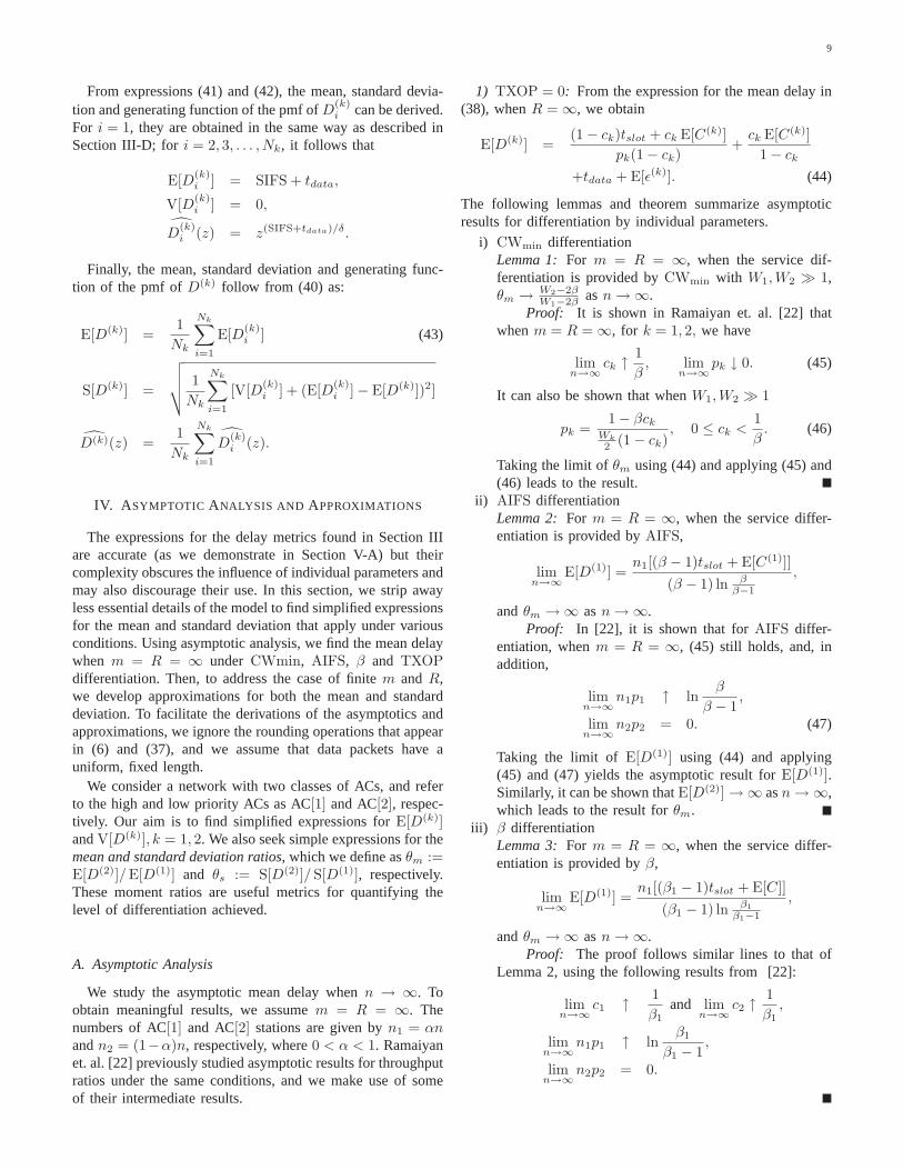
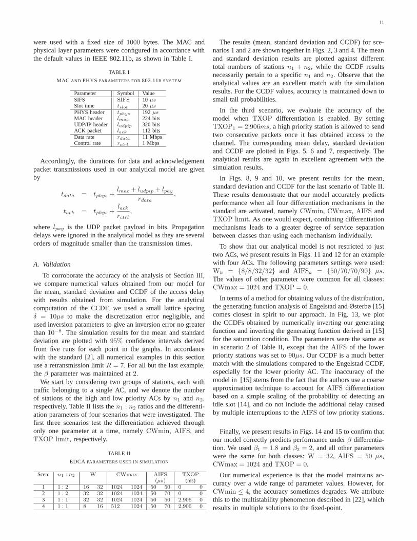
The results (mean, standard deviation and CCDF) for sce-narios 1 and 2 are shown together in Figs. 2, 3 and 4. The meanand standard deviation results are plotted against differenttotal numbers of stationsn1 + n2, while the CCDF resultsnecessarily pertain to a specificn1 and n2. Observe that theanalytical values are an excellent match with the simulationresults. For the CCDF values, accuracy is maintained down tosmall tail probabilities.

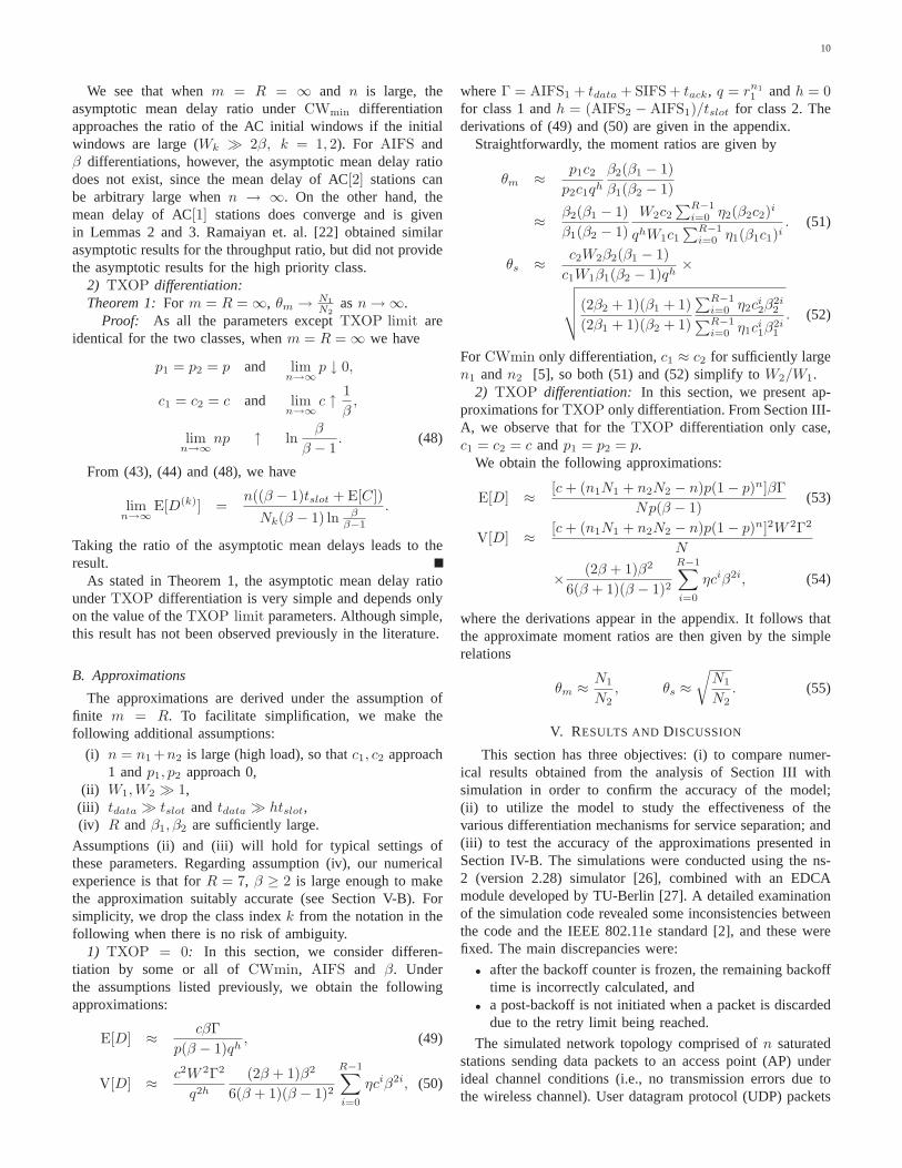
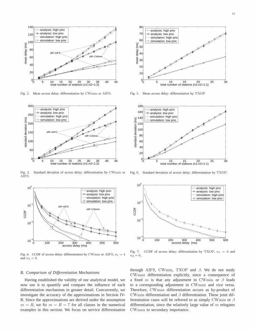
In the third scenario, we evaluate the accuracy of themodel whenTXOP differentiation is enabled. By settingTXOP1 = 2.906ms, a high priority station is allowed to sendtwo consecutive packets once it has obtained access to thechannel. The corresponding mean delay, standard deviationand CCDF are plotted in Figs. 5, 6 and 7, respectively. Theanalytical results are again in excellent agreement with thesimulation results.

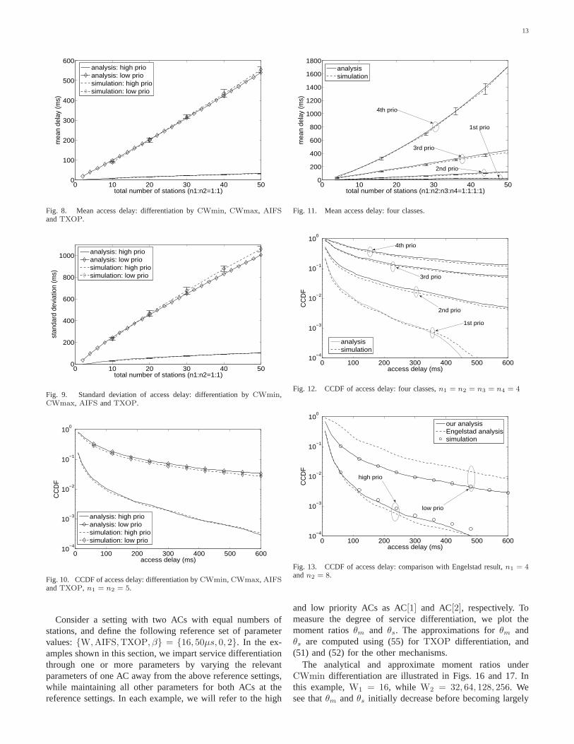
In Figs. 8, 9 and 10, we present results for the mean,standard deviation and CCDF for the last scenario of Table II.These results demonstrate that our model accurately predictsperformance when all four differentiation mechanisms in thestandard are activated, namelyCWmin, CWmax, AIFS andTXOP limit. As one would expect, combining differentiationmechanisms leads to a greater degree of service separationbetween classes than using each mechanism individually.

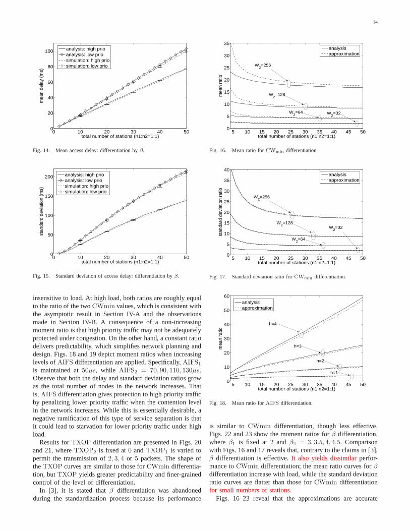
To show that our analytical model is not restricted to justtwo ACs, we present results in Figs. 11 and 12 for an examplewith four ACs. The following parameters settings were used:Wk = {8/8/32/32} and AIFSk = {50/70/70/90} µs.The values of other parameter were common for all classes:CWmax = 1024 andTXOP = 0.

In terms of a method for obtaining values of the distribution,the generating function analysis of Engelstad and Østerbø [15]comes closest in spirit to our approach. In Fig. 13, we plotthe CCDFs obtained by numerically inverting our generatingfunction and inverting the generating function derived in [15]for the saturation condition. The parameters were the same asin scenario 2 of Table II, except that theAIFS of the lowerpriority stations was set to90µs. Our CCDF is a much bettermatch with the simulations compared to the Engelstad CCDF,especially for the lower priority AC. The inaccuracy of themodel in [15] stems from the fact that the authors use a coarseapproximation technique to account forAIFS differentiationbased on a simple scaling of the probability of detecting anidle slot [14], and do not include the additional delay causedby multiple interruptions to theAIFS of low priority stations.

Finally, we present results in Figs. 14 and 15 to confirm thatour model correctly predicts performance underβ differentia-tion. We usedβ1 = 1.8 andβ2 = 2, and all other parameterswere the same for both classes:W = 32, AIFS = 50 µs,CWmax = 1024 andTXOP = 0.

Our numerical experience is that the model maintains ac-curacy over a wide range of parameter values. However, forCWmin ≤ 4, the accuracy sometimes degrades. We attributethis to the multistability phenomenon described in [22], whichresults in multiple solutions to the fixed-point.

12

0 5 10 15 20 25 30 35 40 450

20

40

60

80

100

120

140

total number of stations (n1:n2=1:2)

mea

n de

lay

(ms)

analysis: high prioanalysis: low priosimulation: high priosimulation: low prio

diff−AIFS

diff−CWmin

Fig. 2. Mean access delay: differentiation byCWmin or AIFS.

0 5 10 15 20 25 30 35 40 450

50

100

150

200

250

300

total number of stations (n1:n2=1:2)

stan

dard

dev

iatio

n (m

s)

analysis: high prioanalysis: low priosimulation: high priosimulation: low prio

diff−AIFS

diff−CWmin

Fig. 3. Standard deviation of access delay: differentiation by CWmin orAIFS.

0 100 200 300 400 500 60010

−3

10−2

10−1

100

access delay (ms)

CC

DF

analysis: high prioanalysis: low priosimulation: high priosimulation: low prio

diff−AIFSdiff−CWmin

Fig. 4. CCDF of access delay: differentiation byCWmin or AIFS, n1 = 4andn2 = 8.

B. Comparison of Differentiation Mechanisms

Having established the validity of our analytical model, wenow use it to quantify and compare the influence of eachdifferentiation mechanism in greater detail. Concurrently, weinvestigate the accuracy of the approximations in Section IV-B. Since the approximations are derived under the assumptionm = R, we fix m = R = 7 for all classes in the numericalexamples in this section. We focus on service differentiation

0 5 10 15 20 25 300

10

20

30

40

50

60

70

80

total number of stations (n1:n2=1:1)

mea

n de

lay

(ms)

analysis: high prioanalysis: low priosimulation: high priosimulation: low prio

Fig. 5. Mean access delay: differentiation byTXOP.

0 5 10 15 20 25 300

20

40

60

80

100

120

140

160

180

total number of stations (n1:n2=1:1)

stan

dard

dev

iatio

n (m

s)

analysis: high prioanalysis: low priosimulation: high priosimulation: low prio

Fig. 6. Standard deviation of access delay: differentiation by TXOP.

0 100 200 300 400 500 60010

−3

10−2

10−1

100

access delay (ms)

CC

DF

analysis: high prioanalysis: low priosimulation: high priosimulation: low prio

Fig. 7. CCDF of access delay: differentiation byTXOP, n1 = 6 andn2 = 6.

through AIFS, CWmin, TXOP and β. We do not studyCWmax differentiation explicitly, since a consequence ofa fixed m is that any adjustment inCWmin or β leadsto a corresponding adjustment inCWmax and vice versa.Therefore,CWmax differentiation occurs as by-product ofCWmin differentiation andβ differentiation. These joint dif-ferentiation cases will be referred to as simplyCWmin or βdifferentiation, since the relatively large value ofm relegatesCWmax to secondary importance.

13

0 10 20 30 40 500

100

200

300

400

500

600

total number of stations (n1:n2=1:1)

mea

n de

lay

(ms)

analysis: high prioanalysis: low priosimulation: high priosimulation: low prio

Fig. 8. Mean access delay: differentiation byCWmin, CWmax, AIFSandTXOP.

0 10 20 30 40 500

200

400

600

800

1000

total number of stations (n1:n2=1:1)

stan

dard

dev

iatio

n (m

s)

analysis: high prioanalysis: low priosimulation: high priosimulation: low prio

Fig. 9. Standard deviation of access delay: differentiation by CWmin,CWmax, AIFS andTXOP.

0 100 200 300 400 500 60010

−4

10−3

10−2

10−1

100

CC

DF

access delay (ms)

analysis: high prioanalysis: low priosimulation: high priosimulation: low prio

Fig. 10. CCDF of access delay: differentiation byCWmin, CWmax, AIFSandTXOP, n1 = n2 = 5.

Consider a setting with two ACs with equal numbers ofstations, and define the following reference set of parametervalues:{W,AIFS,TXOP, β} = {16, 50µs, 0, 2}. In the ex-amples shown in this section, we impart service differentiationthrough one or more parameters by varying the relevantparameters of one AC away from the above reference settings,while maintaining all other parameters for both ACs at thereference settings. In each example, we will refer to the high

0 10 20 30 40 500

200

400

600

800

1000

1200

1400

1600

1800

total number of stations (n1:n2:n3:n4=1:1:1:1)

mea

n de

lay

(ms)

analysissimulation

4th prio

3rd prio

1st prio

2nd prio

Fig. 11. Mean access delay: four classes.

0 100 200 300 400 500 60010

−4

10−3

10−2

10−1

100

access delay (ms)

CC

DF

analysissimulation

1st prio

2nd prio

3rd prio

4th prio

Fig. 12. CCDF of access delay: four classes,n1 = n2 = n3 = n4 = 4

0 100 200 300 400 500 60010

−4

10−3

10−2

10−1

100

access delay (ms)

CC

DF

our analysisEngelstad analysissimulation

high prio

low prio

Fig. 13. CCDF of access delay: comparison with Engelstad result, n1 = 4andn2 = 8.

and low priority ACs as AC[1] and AC[2], respectively. Tomeasure the degree of service differentiation, we plot themoment ratiosθm and θs. The approximations forθm andθs are computed using (55) forTXOP differentiation, and(51) and (52) for the other mechanisms.

The analytical and approximate moment ratios underCWmin differentiation are illustrated in Figs. 16 and 17. Inthis example,W1 = 16, while W2 = 32, 64, 128, 256. Wesee thatθm andθs initially decrease before becoming largely

14

0 10 20 30 40 500

20

40

60

80

100

total number of stations (n1:n2=1:1)

mea

n de

lay

(ms)

analysis: high prioanalysis: low priosimulation: high priosimulation: low prio

Fig. 14. Mean access delay: differentiation byβ.

0 10 20 30 40 500

50

100

150

200

total number of stations (n1:n2=1:1)

stan

dard

dev

iatio

n (m

s)

analysis: high prioanalysis: low priosimulation: high priosimulation: low prio

Fig. 15. Standard deviation of access delay: differentiation by β.

insensitive to load. At high load, both ratios are roughly equalto the ratio of the twoCWmin values, which is consistent withthe asymptotic result in Section IV-A and the observationsmade in Section IV-B. A consequence of a non-increasingmoment ratio is that high priority traffic may not be adequatelyprotected under congestion. On the other hand, a constant ratiodelivers predictability, which simplifies network planning anddesign. Figs. 18 and 19 depict moment ratios when increasinglevels ofAIFS differentiation are applied. Specifically,AIFS1

is maintained at50µs, while AIFS2 = 70, 90, 110, 130µs.Observe that both the delay and standard deviation ratios growas the total number of nodes in the network increases. Thatis, AIFS differentiation gives protection to high priority trafficby penalizing lower priority traffic when the contention levelin the network increases. While this is essentially desirable, anegative ramification of this type of service separation is thatit could lead to starvation for lower priority traffic under highload.

Results forTXOP differentiation are presented in Figs. 20and 21, whereTXOP2 is fixed at0 andTXOP1 is varied topermit the transmission of2, 3, 4 or 5 packets. The shape oftheTXOP curves are similar to those forCWmin differentia-tion, butTXOP yields greater predictability and finer-grainedcontrol of the level of differentiation.

In [3], it is stated thatβ differentiation was abandonedduring the standardization process because its performance

5 10 15 20 25 30 35 40 45 500

5

10

15

20

25

30

35

total number of stations (n1:n2=1:1)

mea

n ra

tio

analysisapproximation

W2=256

W2=128

W2=64 W

2=32

Fig. 16. Mean ratio forCWmin differentiation.

5 10 15 20 25 30 35 40 45 500

5

10

15

20

25

30

35

40

total number of stations (n1:n2=1:1)

stan

dard

dev

iatio

n ra

tio

analysisapproximation

W2=256

W2=128

W2=64

W2=32

Fig. 17. Standard deviation ratio forCWmin differentiation.

5 10 15 20 25 30 35 40 45 500

10

20

30

40

50

60

total number of stations (n1:n2=1:1)

mea

n ra

tio

analysisapproximation

h=4

h=2

h=1

h=3

Fig. 18. Mean ratio forAIFS differentiation.

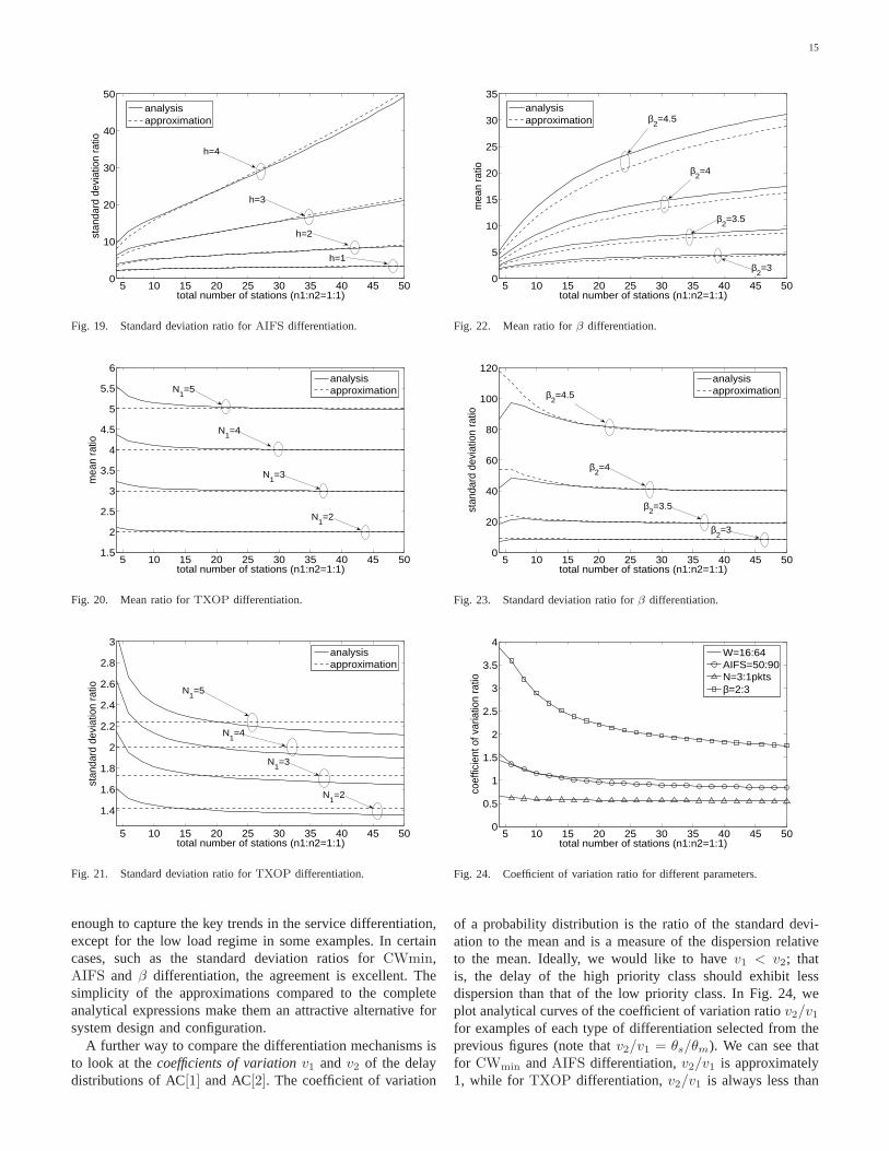
is similar to CWmin differentiation, though less effective.Figs. 22 and 23 show the moment ratios forβ differentiation,where β1 is fixed at 2 and β2 = 3, 3.5, 4, 4.5. Comparisonwith Figs. 16 and 17 reveals that, contrary to the claims in [3],β differentiation is effective.It also yields dissimilarperfor-mance toCWmin differentiation; the mean ratio curves forβdifferentiation increase with load, while the standard deviationratio curves are flatter than those forCWmin differentiationfor small numbers of stations.

Figs. 16–23 reveal that the approximations are accurate

15

5 10 15 20 25 30 35 40 45 500

10

20

30

40

50

total number of stations (n1:n2=1:1)

stan

dard

dev

iatio

n ra

tioanalysisapproximation

h=4

h=3

h=2

h=1

Fig. 19. Standard deviation ratio forAIFS differentiation.

5 10 15 20 25 30 35 40 45 501.5

2

2.5

3

3.5

4

4.5

5

5.5

6

total number of stations (n1:n2=1:1)

mea

n ra

tio

analysisapproximationN

1=5

N1=3

N1=2

N1=4

Fig. 20. Mean ratio forTXOP differentiation.

5 10 15 20 25 30 35 40 45 50

1.4

1.6

1.8

2

2.2

2.4

2.6

2.8

3

total number of stations (n1:n2=1:1)

stan

dard

dev

iatio

n ra

tio

analysisapproximation

N1=5

N1=4

N1=3

N1=2

Fig. 21. Standard deviation ratio forTXOP differentiation.

enough to capture the key trends in the service differentiation,except for the low load regime in some examples. In certaincases, such as the standard deviation ratios forCWmin,AIFS and β differentiation, the agreement is excellent. Thesimplicity of the approximations compared to the completeanalytical expressions make them an attractive alternative forsystem design and configuration.

A further way to compare the differentiation mechanisms isto look at thecoefficients of variationv1 andv2 of the delaydistributions of AC[1] and AC[2]. The coefficient of variation

5 10 15 20 25 30 35 40 45 500

5

10

15

20

25

30

35

total number of stations (n1:n2=1:1)

mea

n ra

tio

analysisapproximation β

2=4.5

β2=4

β2=3.5

β2=3

Fig. 22. Mean ratio forβ differentiation.

5 10 15 20 25 30 35 40 45 500

20

40

60

80

100

120

total number of stations (n1:n2=1:1)

stan

dard

dev

iatio

n ra

tio

analysisapproximationβ

2=4.5

β2=4

β2=3.5

β2=3

Fig. 23. Standard deviation ratio forβ differentiation.

5 10 15 20 25 30 35 40 45 500

0.5

1

1.5

2

2.5

3

3.5

4

total number of stations (n1:n2=1:1)

coef

ficie

nt o

f var

iatio

n ra

tio

W=16:64AIFS=50:90N=3:1pktsβ=2:3

Fig. 24. Coefficient of variation ratio for different parameters.

of a probability distribution is the ratio of the standard devi-ation to the mean and is a measure of the dispersion relativeto the mean. Ideally, we would like to havev1 < v2; thatis, the delay of the high priority class should exhibit lessdispersion than that of the low priority class. In Fig. 24, weplot analytical curves of the coefficient of variation ratiov2/v1

for examples of each type of differentiation selected from theprevious figures (note thatv2/v1 = θs/θm). We can see thatfor CWmin andAIFS differentiation,v2/v1 is approximately1, while for TXOP differentiation,v2/v1 is always less than

16

5 10 15 20 25 30 35 40 45 500

10

20

30

40

50

60

total number of stations (n1:n2=1:1)

mea

n ra

tioW

2=16, h=2

W2=16, h=3

W2=16, h=4

W2=32, h=2

W2=32, h=3

Fig. 25. Mean ratio for jointAIFS andCWmin differentiation.

5 10 15 20 25 30 35 40 45 500

10

20

30

40

50

total number of stations (n1:n2=1:1)

stan

dard

dev

iatio

n ra

tio

W2=16, h=2

W2=16, h=3

W2=16, h=4

W2=32, h=2

W2=32, h=3

Fig. 26. Standard deviation ratio for jointAIFS andCWmin differentiation.

1. In contrast,v2/v1 for β differentiation is greater than 1,so in this respect,β differentiation is superior to the othermechanisms.

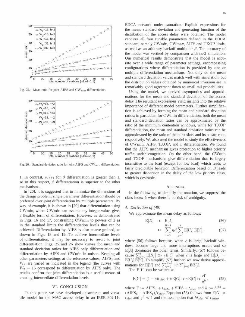
In [20], it is suggested that to minimize the dimensions ofthe design problem, single parameter differentiation should bepreferred over joint differentiation by multiple parameters. Byway of example, it is shown in [20] that differentiation usingCWmin, whereCWmin can assume any integer value, givesa flexible form of differentiation. However, as demonstratedin Figs. 16 and 17, constrainingCWmin to powers of 2 asin the standard limits the differentiation levels that can beachieved. Differentiation byAIFS is also coarse-grained, asshown in Figs. 18 and 19. To achieve intermediate levelsof differentiation, it may be necessary to resort to jointdifferentiation. Figs. 25 and 26 show curves for mean andstandard deviation ratios forAIFS only differentiation anddifferentiation byAIFS and CWmin in unison. Keeping allother parameters settings at the reference values,AIFS2 andW2 are varied as indicated in the legend (the curves withW2 = 16 correspond to differentiation byAIFS only). Theresults confirm that joint differentiation is a useful meansofcreating intermediate differentiation levels.

VI. CONCLUSION

In this paper, we have developed an accurate and versa-tile model for the MAC access delay in an IEEE 802.11e

EDCA network under saturation. Explicit expressions forthe mean, standard deviation and generating function of thedistribution of the access delay were obtained. The modelcaptures all four tunable parameters defined in the EDCAstandard, namelyCWmin, CWmax, AIFS andTXOP limit,as well as an arbitrary backoff multiplierβ. The accuracy ofthe model was verified by comparison with ns-2 simulation.Our numerical results demonstrate that the model is accu-rate over a wide range of parameter settings, encompassingconfigurations where differentiation is provided by one ormultiple differentiation mechanisms. Not only do the meanand standard deviation values match well with simulation, butthe distribution values obtained by numerical inversion are inremarkably good agreement down to small tail probabilities.

Using the model, we derived asymptotics and approxi-mations for the mean and standard deviation of the accessdelay. The resultant expressions yield insights into the relativeimportance of different model parameters. Further simplifica-tion is achieved by forming the mean and standard deviationratios; in particular, forCWmin differentiation, both the meanand standard deviation ratios can be approximated by theratio of the minimum contention windows, while forTXOPdifferentiation, the mean and standard deviation ratios can beapproximated by the ratio of the burst sizes and its square root,respectively. We also used the model to study the effectivenessof CWmin, AIFS, TXOP, and β differentiation. We foundthat theAIFS mechanism gives protection to higher prioritytraffic under congestion. On the other hand, theCWminand TXOP mechanisms give differentiation that is largelyinsensitive to the load (except for low load) which leads tofairly predictable behavior. Differentiation based onβ leadsto greater dispersion in the delay of the low priority class,which is desirable.

APPENDIX

In the following, to simplify the notation, we suppress theclass indexk when there is no risk of ambiguity.

A. Derivation of (49)

We approximate the mean delay as follows:

E[D] ≈ E[A] (56)

≈

R−1∑

i=0

ηcii∑

j=0

E[Uj ] E[Y ], (57)

where (56) follows because, whenc is large, backoff win-dows become large and more interruptions occur, and soE[A] dominates the other terms. Similarly, (57) follows be-cause

∑ij=0 E[Bj ] ≫ iE[C] when c is large andE[Bj ] =

E[Uj ] E[Y ]. To simplify (57) further, we now derive approxi-mations forE[Y ] and

∑R−1i=0 ηci

∑ij=0 E[Uj ].

The E[Y ] can be written as

E[Y ] = (1 − c)tslot + cE[G] ≈ cE[G] ≈cΓ

qh, (58)

whereΓ := AIFS1 + tdata + SIFS + tack, andh := h(k) =(AIFSk −AIFS1)/tslot. Equation (58) follows fromE[G] ≫tslot andqh ≪ 1 and the assumption thathtslot ≪ tdata.

17

We also have

R−1∑

i=0

ηcii∑

j=0

E[Uj ] ≈R−1∑

i=0

ηcii∑

j=0

W

2βj (59)

≈1

β − 1

W

2β

R−1∑

i=0

ηciβi, (60)

where (59) follows under the assumptionW ≫ 1, (60) isobtained because for sufficiently largec andβ, it can be shownthat

β

R−1∑

i=0

ηciβi ≫ 1. (61)

Finally, by substituting (58) and (60) into (57), and usingthe approximation

1

p=

R−1∑

i=0

ηci E[Ui] ≈W

2

R−1∑

i=0

ηciβi, (62)

we obtain (49).

B. Derivation of (50)

We approximate the variance as

V[D] ≈ V[A] (63)

≈

R−1∑

i=0

ηci{

i∑

j=0

V[Bj ] + E[Ai]2} − E[A]2 (64)

≈

R−1∑

i=0

ηcii∑

j=0

E[Uj ] V[Y ] +

R−1∑

i=0

ηcii∑

j=0

V[Uj ] E[Y ]2

+R−1∑

i=0

ηci(i∑

j=0

E[Uj ] E[Y ])2 − E[A]2, (65)

where (63) follows becauseV[A] ≫ V[ǫ] (since c is large),(64) from

∑ij=0 V[Bj ] ≫ V[ǫ].

We then approximateV[Y ] andV[Uj ] as

V[Y ] ≈ c(1 − c) E[G]2 + cV[ǫ] (66)

≈ c(1 − c) E[G]2 + (1 − qh) E[G]2

≈ c(2 − c) E[G]2, (67)

V[Uj ] =β2jW 2 − 1

12≈

W 2

12β2j , (68)

where, (66) is again becauseE[G] ≫ tslot, (67) follows fromqh ≪ 1, and (68) is due toW ≫ 1. To further simplify (65),we note that for largeR and sufficiently largeβ, it can beshown that

R−1∑

i=0

ηciβ2i ≫

R−1∑

i=0

ηciβi, (69)

R−1∑

i=0

ηciβ2i ≫ (

R−1∑

i=0

ηciβi)2. (70)

Based on (61), (69) and (70), and under the assumption thatW ≫ 1, we obtain

R−1∑

i=0

ηcii∑

j=0

V[Uj ] ≈

R−1∑

i=0

ηcii∑

j=0

β2jW 2

12

≈W 2β2

12(β2 − 1)

R−1∑

i=0

ηciβ2i, (71)

R−1∑

i=0

ηci(

i∑

j=0

E[Uj ])2 ≈

R−1∑

i=0

ηci(

i∑

j=0

W

2βj)2

≈W 2β2

4(β − 1)2

R−1∑

i=0

ηciβ2i. (72)

Finally, substituting (57), (58), (60), (67), (68), (71) and (72)into (65), and using the fact of (69) and (70), we obtain

V[D] ≈W 2β2

12(β2 − 1)c2 E[G]2

R−1∑

i=0

ηciβ2i

+W 2β2

4(β − 1)2c2 E[G]2

R−1∑

i=0

ηciβ2i (73)

≈c2W 2Γ2

q2h

(2β + 1)β2

6(β + 1)(β − 1)2

R−1∑

i=0

ηciβ2i. (74)

C. Derivation of (53) and (54)

The mean delay is given by

E[D] ≈E[D1]

N(75)

≈E[Y ]

∑R−1i=0 ηci

∑ij=0 E[Uj ]

N, (76)

where (75) follows becauseE[D1] ≫ (N − 1)(SIFS + tdata)when c is sufficiently large, and (76) comes from (57). WeapproximateE[Y ] as follows:

E[Y ] = (1 − c)tslot + γ1 E[G1] + γ2 E[G2] + ν E[H]

≈ [c + (n1N1 + n2N2 − n)p(1 − p)n] Γ, (77)

whereΓ := tdata + SIFS + tack + AIFS (note thatAIFS =AIFS1 = AIFS2 for TXOP only differentiation).

Substituting (60) and (77) into (76), and making use of (62),yields (53).

The variance of the access delay can be simplified as:

V[D] ≈V[D1] + N−1

N E[D1]2

N(78)

≈V[D1] + E[D1]

2

N(79)

≈

∑R−1i=0 ηci{

∑ij=0 V[Bj ] + E[Ai]

2}

N, (80)

≈(2β + 1)β2

6(β + 1)(β − 1)2W 2 E[Y ]2

N

R−1∑

i=0

ηciβ2i,(81)

where (78) is obtained using the fact thatE[D1] ≫ tdata +SIFS, (79) follows fromN(V[D1] + E[D1]

2) ≫ E[D1]2 for

sufficiently largeβ, (80) follows from (56) and (64), and (81)is obtained via similar arguments that led from (64) to (74).Finally, substituting (77) into (81) leads to (54).

18

REFERENCES

[1] IEEE, IEEE 802.11 Part 11: Wireless LAN Medium Access Control(MAC) and Physical Layer (PHY) Specifications, 1999.

[2] ——, IEEE 802.11 Part 11: Wireless LAN Medium Access Control(MAC) and Physical Layer (PHY) Specifications, Amendment 8:MediumAccess Control (MAC) Quality of Service Enhancements, 2005.

[3] G. Bianchi, I. Tinnirello, and L. Scalia, “Understanding 802.11econtention-based prioritization mechanisms and their coexistence withlegacy 802.11 stations,”IEEE Network, vol. 19, No. 4, pp. 28–34, 2005.

[4] T. Sakurai and H. L. Vu, “Access delay of the IEEE 802.11 MAC proto-col under saturation,”IEEE Transactions on Wireless Communications,vol. 6, No.5, pp. 1702–1710, 2007.

[5] D. Xu, T. Sakurai, and H. L. Vu, “An analytical model of MAC accessdelay in IEEE 802.11e EDCA,”Proc. IEEE Wireless Communicationsand Networking Conference, vol. 4, pp. 1938–1943, 2006.

[6] ——, “MAC access delay in IEEE 802.11e EDCA,”Proc. IEEE 64thVehicular Technology Conference - Fall, 2006.

[7] Y. Xiao, “Performance analysis for priority schemes for IEEE 802.11and IEEE 802.11e wireless LANs,”IEEE Transactions on WirelessCommunications, vol. 4, no. 4, pp. 1506–1515, 2005.

[8] Z. Kong, D. H. Tsang, B. Bensaou, and D. Gao, “Performance analysisof IEEE 802.11e contention-based channel access,”IEEE Journal onSelected Areas in Communications, vol. 22, no. 10, pp. 2095–2106,2004.

[9] J. Tantra, C. H. Foh, and A. Mnaouer, “Throughput and delay analysisof the IEEE 802.11e EDCA saturation,”Proc. IEEE InternationalConference on Communications, vol. 5, pp. 3350–3454, 2005.

[10] X. Tao and S. Panwar, “Throughput and delay analysis forthe IEEE802.11e enhanced distributed channel access,”IEEE Transactions onCommunications, vol. 54, no. 4, pp. 596–603, 2006.

[11] T.-C. Tsai and M.-J. Wu, “An analytical model for IEEE 802.11eEDCA,” Proc. IEEE International Conference on Communications,vol. 5, pp. 3474–3478, 2005.

[12] J. Hui and M. Devetsikiotis, “A unified model for the performance analy-sis of IEEE 802.11e EDCA,”IEEE Transactions on Communications,vol. 53, no. 9, pp. 1498–1510, 2005.

[13] H. Zhu and I. Chlamtac, “Performance analysis for IEEE 802.11e EDCFservice differentiation,”IEEE Transactions on Wireless Communica-tions, vol. 4, no. 4, pp. 1779–1788, 2005.

[14] P. E. Engelstad and O. N. Østerbø, “Non-saturation and saturationanalysis of IEEE 802.11e EDCA with starvation prediction,”Proc. the8th ACM International Symposium on Modeling Analysis and Simulationof Wireless and Mobile Systems (ACM MSWiM), pp. 224–233, 2005.

[15] ——, “Analysis of the total delay of IEEE 802.11e EDCA and802.11DCF,” IEEE International Conference on Communications, vol. 2, pp.552–559, 2006.

[16] J.-D. Kim and C.-K. Kim, “Performance analysis and evaluation of IEEE802.11e EDCF,”Wireless Communications and Mobile Computing, vol.4, no. 1, pp. 55–74, 2004.

[17] J. W. Robinson and T. S. Randhawa, “Saturation throughput analysisof IEEE 802.11e enhanced distributed coordination function,” IEEEJournal on Selected Areas in Communications, vol. 22, no. 5, pp. 917–928, 2004.

[18] ——, “A practical model for transmission delay of IEEE 802.11e en-hanced distributed channel access,”Proc. IEEE International Personal,Indoor and Mobile Radio Communications (PIMRC), vol. 1, pp. 323–328, 2004.

[19] F. Peng, H. M. Alnuweiri, and V. C. M. Leung, “Analysis ofbursttransmission in IEEE 802.11e wireless LANs,”Proc. IEEE InternationalConference on Communications, vol. 2, pp. 535–539, 2005.

[20] Y. Ge, J. C. Hou, and S. Choi, “An analytic study of tuningsystemsparameters in IEEE 802.11e enhanced distributed channel access,”Computer Networks, vol. 51, No. 8, pp. 1955–1980, 2007.

[21] G. Bianchi, “Performance analysis of the IEEE 802.11 distributed coor-dination function,”IEEE Journal on Selected Areas in Communications,vol. 18, no. 3, pp. 535–547, 2000.

[22] V. Ramaiyan, A. Kumar, and E. Altman, “Fixed point analysisof singlecell IEEE 802.11e WLANs: Uniqueness, multistability and throughputdifferentiation,” Proc. SIGMETRICS’05, 2005.

[23] S. Mangold, S. Choi, G. R. Hiertz, O. Klein, and B. Walke,“Analysisof IEEE 802.11e for QoS support in wireless LANs,”IEEE WirelessCommunications, vol. 10, no. 6, pp. 40–50, Dec. 2003.

[24] B.-J. Kwak, N.-O. Song, and L. Miller, “Performance analysis ofexponential backoff,”IEEE/ACM Transactions on Networking, vol. 13,no. 2, pp. 343–355, 2005.

[25] J. Abate, G. L. Choudhury, and W. Whitt, “An introductionto numericaltransform inversion and its application to probability models,” in Com-putational Probability, W. K. Grassman, Ed. Norwell, MA: Kluwer,2000, pp. 257–323.

[26] “The network simulator ns-2,” Available athttp://www.isi.edu/nsnam/ns/.

[27] S. Wietholter and C. Hoene, “An IEEE 802.11e EDCFand CFB simulation model for ns-2,” Available athttp://www.tkn.tu-berlin.de/research/802.11e_ns2/.