Stochastic Analysis of Periodic Real-Time Systems

Stochastic Analysis of Periodic Real-Time Systems∗*

Jose Luis Dıaz† Daniel F. Garcıa† Kanghee Kim‡ Chang-Gun Lee¶

Lucia Lo Bello§ Jose Marıa Lopez† Sang Lyul Min‡ Orazio Mirabella§

Abstract

This paper describes a stochastic analysis method forgeneral periodic real-time systems. The proposed methodaccurately computes the response time distribution of eachtask in the system, thus making it possible to determinethe deadline miss probability of individual tasks, even forsystems with maximum utilization factor greater than one.The method uniformly covers both fixed-priority schedul-ing (such as Rate Monotonic) as well as dynamic-priorityscheduling (such as Earliest Deadline First) and can han-dle arbitrary relative deadlines and execution time distribu-tions. The accuracy of the method is proven by comparingthe results from the analysis with those obtained from sim-ulations, as well as other methodologies in the literature.

1. Introduction

Traditional scheduling algorithms and analysis methods,such as processor utilization analysis [16, 11] and responsetime analysis [4, 19], focus on strict “hard” deadlines, bywhich a system is deemed schedulable only if every in-stance (called a job) of every task is guaranteed to meet its

* The author names are listed in alphabetical order since this paper isa collaborative work based on two different papers submitted to the con-ference separately. One paper was written by Jose Luis Dıaz, Jose MarıaLopez and Daniel F. Garcıa, and the other was written by Kanghee Kim,Lucia Lo Bello, Chang-Gun Lee, Sang Lyul Min, and Orazio Mirabella.

† Jose Luis Dıaz, Jose Marıa Lopez and Daniel F. Garcıa({jdiaz,chechu,daniel}@atc.uniovi.es ), Departamento deInformatica, Universidad de Oviedo(33204, Gijon, Spain)

‡ Kanghee Kim ([email protected] ) and Sang Lyul Min([email protected] ), School of Computer Science andEngineering, Seoul National University(Shillim-dong San 56-1, Kwanak-Gu, Seoul, 151-742 Korea), supported in part by the Ministry of Scienceand Technology under the National Research Laboratory program and bythe Ministry of Education under the BK21 program

§ Lucia Lo Bello and Orazio Mirabella ({llobello,omirabel}@diit.unict.it ), Dipartimento di Ingegneria Informatica e delle Tele-comunicazioni, Facolta di Ingegneria, Universita di Catania(Viale A. Do-ria 6, 95125 Catania, Italy)

¶ Chang-Gun Lee ([email protected] ), Depart-ment of Electrical Engineering, Ohio State University(2015 Neil Avenue,Columbus, OH 43210, U.S.A.)

deadline. Although this deterministic timing guarantee isneeded in hard real-time systems, it is too stringent for so-called soft real-time applications that require only a prob-abilistic guarantee that the deadline miss ratio of a task isbelow a given threshold. For such soft real-time applica-tions, we need to relax the assumption that every instanceof a task requires the worst-case execution time and analyzesystem behavior from a statistical point of view.

Progress has recently been made in the analysis of real-time systems under the stochastic assumption that jobs froma task require variable execution times. Research in thisarea can be categorized into two groups depending on theapproach it takes to facilitate the analysis. The methods inthe first group introduce a worst-case assumption to sim-plify the analysis (e.g., the critical instant assumption inProbabilistic Time Demand Analysis [18] and StochasticTime Demand Analysis [7, 6]) or a restrictive assumption(e.g., the heavy traffic condition in the Real-Time QueueingTheory [12, 13]). Those in the second group, on the otherhand, assume a special scheduling model that provides iso-lation between tasks so that each task can be analyzed inde-pendently of other tasks in the system (e.g., the reservation-based system addressed in [1] and Statistical Rate Mono-tonic Scheduling [2]).

In this paper, we propose a stochastic analysis methodthat does not introduce any worst-case or restrictive as-sumptions into the analysis, and is applicable to generalpriority-driven real-time systems. The method is generalin the sense that it covers general priority-driven systemsincluding both fixed-priority systems such as RM [16] andDM [15] and dynamic-priority systems such as EDF [16](First In First Out is also covered since it is considered aspecial case of EDF where all the jobs have a constant rela-tive deadline). The analysis method can handle any periodictask set consisting of tasks with arbitrary relative deadlines(including relative deadlines greater than the periods) andarbitrary execution time distributions.

The analysis method is based on Markov process mod-eling, which enables us to reason probabilistically aboutthe steady-state behavior of the system even in the case ofpossible overload. It provides both analytical and numeri-cal solutions for the deadline miss probabilities of tasks by

Proceedings of the 23rd IEEE REAL-TIME SYSTEMS SYMPOSIUM (RTSS’02) 1052-8725/02 $17.00 © 2002 IEEE

computing the complete probability function (PF) of the re-sponse time of each task.

The rest of the paper is organized as follows. In Sec-tion 2, the related work is described in detail. In Section 3,the system model assumed and the notations used through-out the paper are given. Section 4 describes the stochas-tic analysis method we propose and also explains variousapproximation techniques to reduce its computational over-heads. In Section 5, we compare experimental results fromthe proposed analysis method with those obtained from sim-ulations and other methodologies. Finally, in Section 6, weconclude the paper with directions for future research.

2. Related work

Several studies have addressed the variability of task ex-ecution times even in deterministic schedulability analysis.For example, a multiframe model was proposed by Mokand Chen [17] in which the execution time of a task mayvary greatly from one instance to another assuming that thisvariation follows a known pattern. The pattern is given asa finite list of numbers, and the execution times of succes-sive instances are generated from the list. From this model,new utilization bounds which improve those of Liu and Lay-land [16] are derived for fixed-priority preemptive schedul-ing. However, since this model is aimed at providing a de-terministic timing guarantee, it is still pessimistic.

In the attempt to provide probabilistic guarantees to real-time tasks with variable execution times, some reservation-based models that provide isolation between tasks havebeen studied. These models include the reservation-basedsystem addressed by Abeni and Buttazzo [1] and a modi-fication of Rate Monotonic Scheduling proposed by Atlasand Bestavros [2], which is called Statistical Rate Mono-tonic Scheduling (SRMS). Both assume reservation-basedscheduling algorithms so that the analysis can be performedas if each task had a dedicated (virtual) processor. Thatis, for each task, a guaranteed budget of processor time isprovided in every period [1] or super-period (the period ofthe next low-priority task which is assumed to be an integermultiple of the period of the task in SRMS) [2]. There-fore, the deadline miss probability of a task can be analyzedindependently of other tasks assuming the guaranteed bud-get. However, the stochastic analysis methods developedfor these systems are not applicable to general priority-driven systems due to the adoption of non-priority-drivenscheduling algorithms or the modification of the originalpriority-driven scheduling rules.

A more general approach is to model the system as asingle server queue, and try to apply the results of classi-cal queueing theory. The real-time system we are trying toanalyze is made up of periodic independent tasks scheduledby a preemptive priority-driven scheduler on a uniprocessor.

Apparently, this system is a multiclass queue in which eachclass has deterministic inter-arrival times and arbitrary ser-vice times (D/G/1). However, this model cannot account forthe relative phases of the tasks, which influence the statisti-cal distribution of the response times. Furthermore, the fewresults available for multiclass queues assume specific dis-tributions (Poisson, normal, etc.) for the inter-arrival times.The case of general distributions of inter-arrival times isusually addressed under “heavy-traffic” conditions (i.e., theaverage utilization is close to one) and, even in this case,the results are not valid for deterministic inter-arrival times,because this is a special case of a general distribution.

One extension of the classical queueing theory to dealwith real-time issues was proposed in the Real-Time Queue-ing Theory [12]. This analysis method is flexible in that itis not limited to a particular scheduling algorithm and canbe extended to real-time queueing networks. However, theanalysis method assumes that the system is under heavy-traffic conditions. In addition, it only considers one classof clients, i.e., the interarrival times and execution times areidentically distributed for all the tasks. This model does notfit well with the periodic task model.

Another approach to the statistical characterization ofreal-time systems is to extend an existing response timeanalysis, substituting the fixed execution times with ran-dom variables. Following this approach, Tia et al. [18]proposed the Probabilistic Time Demand Analysis (PTDA),which substitutes the sums of fixed execution times in theTime Demand Analysis [14] with convolutions of probabil-ity functions (PFs). In this way they can obtain the PF of theresponse time of a task assuming the worst-case scenario onthe task release times, i.e., the critical instant. The analy-sis is restricted to the first activation of the task, since thedeadlines cannot be greater than the periods. This assump-tion is also made in the Stochastic Time Demand Analysis(STDA) by Gardner [6], which extends the PTDA to coversystems where the deadlines may be greater than the peri-ods. In this analysis, the probability of deadline misses iscomputed for each job released in the first in-phase busy in-terval, and the maximum of these probabilities is chosen asan upper bound on the probability of deadline misses for thecorresponding task. Both analyses are based on the sum ofrandom variables, and thus the use of convolutions to deter-mine its PF. However, the analyses cannot address systemswhere the maximum system utilization is greater than one.In this case, the assumption that the busy interval startingat the critical instant will contain the worst-case responsetime is no longer valid, so the deadline miss probabiltiescomputed by the analyses are not actual bounds.

Recently, Kim et al. [9] analyzed the stochastic behav-ior of a dynamic-priority system combined with an over-run handling mechanism calledrandomized dropping. Al-though this stochastic analysis method was developed to

Proceedings of the 23rd IEEE REAL-TIME SYSTEMS SYMPOSIUM (RTSS’02) 1052-8725/02 $17.00 © 2002 IEEE

compute the deadline miss probabilities of tasks for sucha system, it can still be used for a “pure” dynamic-prioritysystem. By modeling the system as a Markov process, itcomputes the stationary response time distributions of allthe jobs in a hyperperiod (which is defined as a periodwhose length is equal to the least common multiple of theperiods of all the tasks) and thus the response time distri-butions of all the tasks. However, it deals with dynamic-priority systems only and the derivation of the Markov ma-trix is complicated due to the abstraction ofjob groupsandaggregated response times.

In this paper, we present a broader approach, which startsfrom the ideas of [18], [6] and [9]. We provide a simplederivation method for the Markov matrix and both analyti-cal and numerical solutions for the response time distribu-tions of all the tasks. We also describe a generalized frame-work to deal with both fixed-priority and dynamic-prioritysystems extending the concept presented in [9]. This modelcan be more easily understood starting from a simpler one,in which the system is not seen as a set of periodic tasks,but as a set of jobs released in a given sequence. Basedon the simpler model, a systematic method to compute theresponse time PF of any job is developed and precisely de-scribed in [5, 8]. In Section 4.1, we will summarize thismethod in the more general context of a periodic task sys-tem, and will provide an overview of the whole stochasticanalysis. Finally, note that our stochastic analysis is use-ful not only for soft real-time systems, but also for so-calledprobabilistic hard real-time systems[3], where a probabilis-tic guarantee close to 100% suffices.

3. System model and notation

The system is modeled as a set ofN independent peri-odic tasksS= {τ1,τ2, ...,τN}, each taskτi being modeledby (Ti ,Φi ,Ci ,Di), whereTi is the period of the task,Φi

its initial phase,Ci its execution time, andDi its relativedeadline. The execution time is a discrete random vari-able* with a known probability function (PF), denoted byfCi

(·), where fCi(c) = P{Ci =c}. Since the value ofCi is

bounded, its PF can be stored as a finite vector of values[ fCi

(Cmini ), . . . , fCi

(Cmaxi )].

Each task gives rise to an infinite sequence of jobs, andwe will denote thej-th job of taskτi by Γi, j . The releasetime of jobΓi, j will be denoted byλi, j . This time is deter-ministic and equal toΦi +( j−1)×Ti . Each job requires anexecution time which is a random variable whose distribu-tion is given by fCi

(·), and it is assumed to be independentof other jobs of the same task and those of other tasks.

The scheduling policy we assume is a general priority-driven one that assigns each jobΓi, j a static priority and

* Throughout this paper we use a calligraphic typeface to denote randomvariables, likeC, R, etc.

schedules jobs according to this priority. The schedulerguarantees that the running job is the one with the highestpriority among the ready jobs. We are not concerned withthe policy used to assign priorities to jobs, as long as theyare assigned in a deterministic way. This model includeswell-known policies such asRate Monotonic(RM), Dead-line Monotonic(DM) and Earliest Deadline First(EDF).For fixed-priority policies, we will usePi to denote the pri-ority assigned to taskτi .

The response time of the jobΓi, j will be represented byRi, j . This is a random variable, which can take differentvalues with different probabilities. In the next section weoutline a procedure which allows us to find the probabilityof occurrence of each possible response time for a givenjob, i.e. the probability function (PF) of the response time:fRi, j

(r) = P{Ri, j =r}From the job response time PFs, the response time PF for

any task can be obtained as the average of the response timePFs of the jobs belonging to that task. The task responsetime PF provides the analyst with significant informationabout the stochastic behavior of the system. In particular, itcan be used to compute the probability of deadline missesfor each task. The deadline miss probabilityDMPτi of taskτi can be computed from its response time PF as follows:

DMPτi = P{Rτi>Di}= 1−P{Rτi

≤Di}

4. Stochastic analysis

4.1. Overview

To compute the response time PF of each task, we haveto know the response time PFs of the jobs belonging to it.However, since the number of jobs generated by a task maybe infinite, it is not possible to consider all of them for com-putation of its response time PF. To address this problem,we observe that the arrival pattern of jobs within a hyperpe-riod is repeated for all the other hyperperiods. Thus, if somestochastic regularity is found at the hyperperiod level, wecan restrict our analysis to a single hyperperiod, and say thatthe derived job response time PFs are applicable for otherhyperperiods. In this case, the response time PFfRτi

(·) oftaskτi is represented by the average of the response timePFs of all the jobs from the task in the hyperperiod. That is,

fRτi(r) =

1mi

mi

∑j=1

fRi, j(r) (1)

wheremi = T/Ti is the number of jobs fromτi released in ahyperperiod of lengthT.

To address stochastic regularity in hyperperiods, we firstdefine theP-level backlogobserved at timet as the sumof the remaining execution times of all the jobs that have

Proceedings of the 23rd IEEE REAL-TIME SYSTEMS SYMPOSIUM (RTSS’02) 1052-8725/02 $17.00 © 2002 IEEE

priorities higher than or equal toP and are not completedup to the timet. This random quantity is denoted byWP

t .Then, we focus on theP-level backlog observed at the be-ginning of each hyperperiodk, denoted byBP

k = WPkT, and

investigate the stochastic process defined as the sequence ofrandom variables{BP

1 ,BP2 , ...,BP

k , ...}. We prove that thisstochastic process is a Markov chain. In addition, a sta-tionary distribution of theP-level backlogBP

k exists as longas the stability condition whereby the average system uti-lization is less than one is met. By deriving the Markovmatrix that gives the transition probabilityP{(BP

k = t1) →(BP

k+1 = t2) } for any two statest1 andt2, we compute theexact stationaryP-level backlog PFf

BPk(·), observed at the

beginning of the hyperperiod.*

Once the stationaryP-level backlog PFfBP

k(·) is given,

the stationaryP-level backlog PF observed at any timewithin the hyperperiod can easily be calculated using themethod explained in [5, 8]. Basically, by using two sim-ple operations calledconvolutionandshrinking, theP-levelbacklog PF f

WPt′(·) at any timet ′(> t) can be calculated

from theP-level backlog PFfWP

t(·) at timet. For example,

let us assume a simple scenario in which a job with a prior-ity higher than or equal toP is released at timet and there isno further release of jobs with a priority higher than or equalto P in the interval [t, t ′). In this case, theP-level backlogPF observed immediately after the release of the job, i.e.,fWP

t+(·), is obtained by performing convolution between

fWP

t(·) and the execution time PF of the job. Then, the

P-level backlog PFfWP

t′(·) at timet ′ is obtained by shrink-

ing fWP

t+(·), that is, shiftingf

WPt+

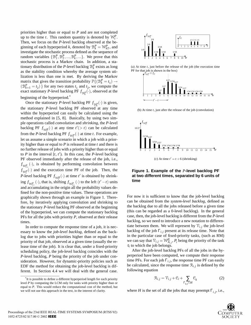
(·) to the left(t ′ − t) unitsand accumulating in the origin all the probability values de-fined for the non-positive time values. These operations aregraphically shown through an example in Figure 1. There-fore, by iteratively applying convolution and shrinking tothe stationaryP-level backlog PF observed at the beginningof the hyperperiod, we can compute the stationary backlogPFs for all the jobs with priorityP, observed at their releasetimes.

In order to compute the response time of a job, it is nec-essary to know thejob-level backlog, defined as the back-log due to jobs with priorities higher than or equal to thepriority of that job, observed at a given time (usually the re-lease time of the job). It is clear that, under a fixed-priorityscheduling policy, the job-level backlog coincides with theP-level backlog,P being the priority of the job under con-sideration. However, for dynamic-priority policies such asEDF the method for obtaining the job-level backlog is dif-ferent. In Section 4.4 we will deal with the general case.

* It is possible to define a different hyperperiod length for each prioritylevel P by computing the LCM only for tasks with priority higher than orequal toP. This would reduce the computational cost of the method, butwe will not use this approach in the text, in the interest of clarity.

fWP

t

w0 1 2 3 4 5 6 7 8 9 10

1/9

2/9

3/9

1/18

3/18

1/18 1/18

fC

r0 1 2 3 4 5 6 7 8

1/3 1/3 1/3

(a) At time t, just before the release of the job (the execution timePF for that job is shown in the box)

fWP

t⊗ fC

w0 1 2 3 4 5 6 7 8 9 10 11 12 13 14 15 16

t ′ − t

1/27

3/27

6/2711/545/27

5/54 2/27

1/54 1/54 1/54 1/54

(b) At time t, just after the release of the job (convolution)

fWP

t′

w0 1 2 3 4 5 6 7 8 9 10 11 12 13 14 15

10/27

11/545/27

5/54 2/271/54 1/54 1/54 1/54

(c) At time t ′ = t +6 (shrinking)

Figure 1. Example of the P-level backlog PFat two different times, separated by 6 units oftime

For now it is sufficient to know that the job-level backlogcan be obtained from thesystem-level backlog, defined asthe backlog due to all the jobs released before a given time(this can be regarded as a 0-level backlog). In the generalcase, then, the job-level backlog is different from theP-levelbacklog, so we need to introduce a new notation to differen-tiate between them. We will represent byVi, j the job-levelbacklog of the jobΓi, j present at its release time. Note thatin the particular case of fixed-priority tasks, (such as RM)we can say thatVi, j = WPi

λi, j, Pi being the priority of the task

τi to which the job belongs.After the job-level backlog PFs of all the jobs in the hy-

perperiod have been computed, we compute their responsetime PFs. For each jobΓi, j , the response time PF can easilybe calculated, since the response timeRi, j is defined by thefollowing equation

Ri, j = Vi, j +Ci + ∑Γk,l∈H

Ck (2)

whereH is the set of all the jobs that may preemptΓi, j , i.e.,

Proceedings of the 23rd IEEE REAL-TIME SYSTEMS SYMPOSIUM (RTSS’02) 1052-8725/02 $17.00 © 2002 IEEE

the set of jobs released after timeλi, j with a priority higherthan that of jobΓi, j . Thus, the stationary response time PFfRi, j

(·) of Γi, j can be computed from the stationary job-levelbacklog PFfVi, j

(·) and the execution time PFfCi(·) of Γi, j

and the execution time PFs of the higher-priority jobs thatpreemptΓi, j .

The response time PF is computed as follows. LetΓ′k bethek-th job inH (we assumeH to be ordered by the releasetimes), andλ ′

k the time that has elapsed between the releaseof Γi, j and that ofΓ′k. First, we calculate the response timePF not considering any possible preemptions by the higher-priority jobs by convolving the job-level backlog PFfVi, j

(·)and the execution time PFfCi

(·) of the jobΓi, j . Then, it-eratively, we calculate the response time PF that reflects allpossible preemptions byΓ′1, Γ′2, ...,Γ′k, ... by convolving theexecution time PFs ofΓ′k’s, in turn (k = 1,2,3, ...), into theresponse time PF ofΓi, j . At each step, sayk, the convolu-tion is applied to the tail part of the response time PF beingcalculated, which is defined in the range (λ ′

k, ∞), since thehigher-priority jobΓ′k may affectΓi, j only if Γi, j executesup to the release time ofΓ′k. In other words, at stepk, theresponse time PF ofΓi, j is calculated by (1) splitting theresponse time PF obtained at stepk−1 into the tail part de-fined for the range (λ ′

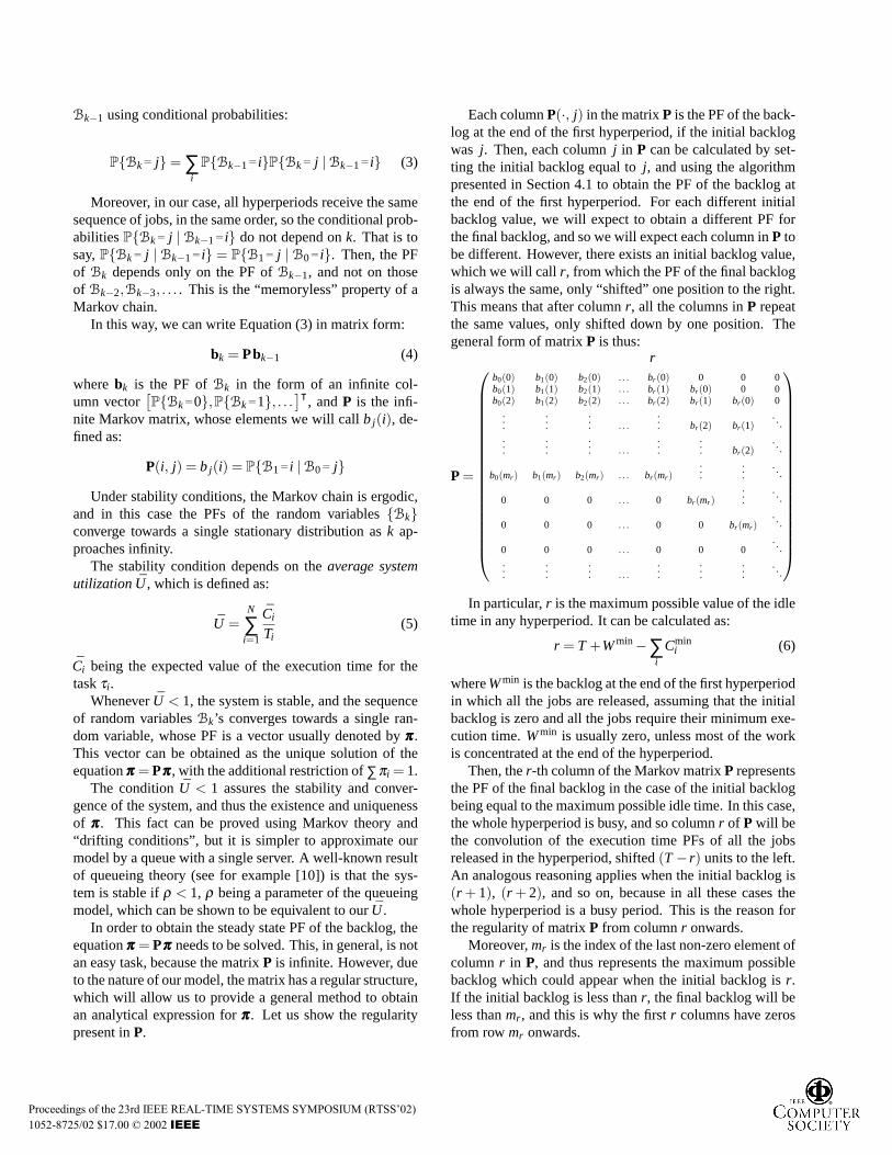
k, ∞) and the remaining head part, (2)convolving the tail part and the execution time PFC′k of Γ′k,and finally (3) merging the head part and the new tail partresulting from the convolution. Figure 2 shows this processgraphically, for thek-th higher-priority job.

This process can also be more formally expressedthrough the following notation: letf I (·) be a partial PF de-fined as the part of the PFf (·) which takes values in theintervalI , as follows.

f I (r) ={

f (r) if r ∈ I0 otherwise

Also, letR<k>i, j be a random variable describing the response

time of job Γi, j that reflects all possible preemptions bythe higher-priority jobsΓ′1,Γ′2, . . . , Γ′k that can preemptΓi, j

(λ ′1 ≤ λ ′

2 ≤ ·· · ≤ λ ′k). Then the response time PFf

R<k>i, j

(·)

can be calculated from the response time PFfR<k−1>

i, j(·) and

the execution time PFfC′k

(·) of Γ′k as follows:

fR<k>

i, j(r) = f [0,λ ′k]

R<k−1>i, j

(r)+( f (λ ′k,∞)R<k−1>

i, j

⊗ fC′k

)(r)

However, in order to obtain the deadline miss probabilityfor each jobΓi, j , it is not necessary to calculate the completeresponse time PF, becauseP{Ri, j >Di} = 1−P{Ri, j ≤Di},and the probabilityP{Ri, j ≤Di} can be computed from thepart of the response time PF defined in the range [0,Di ].If, at stepk, we find thatDi ≤ λ ′

k in the calculation of theresponse time PF, the calculation process can be stopped,

fR<k−1>

i, j

r0 1 2 3 4 5 6 7 8 9

1/4 1/4

1/8

1/4

1/8

f [0,λ ′k]R<k−1>

i, j

r0 1 2 3 4 5 6 7 8 9

1/4 1/4

1/8

1/4

f (λ ′k,∞)R<k−1>

i, j

r0 1 2 3 4 5 6 7 8 9

1/8

λ ′k

(a) “Splitting” the response time PF obtained in stepk−1

fR<k>

i, j

r0 1 2 3 4 5 6 7 8 9 10 11 12

1/4 1/4

1/8

1/4

124

124

124

f [0,λ ′k]R<k−1>

i, j

r0 1 2 3 4 5 6 7

1/4 1/4

1/8

1/4

f (λ ′k,∞)R<k−1>

i, j⊗ fCk

r0 1 2 3 4 5 6 7 8 9 10 11

124

124

124

(b) Construction of the response time PF for stepk

Figure 2. Response time PF calculation

and the exact deadline miss probability can be computed.Moreover, the calculation process can also be stopped whenthe response time PF obtained at some stepk reveals thatthe job Γi, j has a null probability of being running up tothe release time of the next higher-priority jobΓ′k+1 (i.e.,f (λ ′k,∞)R<k>

i, j

(·) is zero).

In the following subsection, we will describe how tocompute the stationaryP-level (or system-level) backlog PFobserved at the beginning of the hyperperiod, and then ex-plain how to deal with dynamic-priority systems such asEDF in the job-level backlog PF computation. In the fol-lowing description, note that, whenever we omit the super-scriptP in BP

k , a priority levelP is implicit in the notation.

4.2. Markovian modeling and stability

The backlog at the beginning of thek-th hyperperiod is arandom variable, whose distribution, in general, is differentfor eachk. So, the sequence of random variables{Bk} is arandom process, which we will call the “backlog process”.We will show that this process is a Markov chain.

The PF ofBk can be expressed in terms of the PF of

Proceedings of the 23rd IEEE REAL-TIME SYSTEMS SYMPOSIUM (RTSS’02) 1052-8725/02 $17.00 © 2002 IEEE

Bk−1 using conditional probabilities:

P{Bk= j}= ∑i

P{Bk−1= i}P{Bk= j |Bk−1= i} (3)

Moreover, in our case, all hyperperiods receive the samesequence of jobs, in the same order, so the conditional prob-abilitiesP{Bk= j | Bk−1= i} do not depend onk. That is tosay,P{Bk= j | Bk−1= i} = P{B1= j | B0= i}. Then, the PFof Bk depends only on the PF ofBk−1, and not on thoseof Bk−2,Bk−3, . . . . This is the “memoryless” property of aMarkov chain.

In this way, we can write Equation (3) in matrix form:

bk = Pbk−1 (4)

wherebk is the PF ofBk in the form of an infinite col-umn vector

[P{Bk=0},P{Bk=1}, . . .

]ᵀ, andP is the infi-

nite Markov matrix, whose elements we will callbj(i), de-fined as:

P(i, j) = bj(i) = P{B1= i |B0= j}

Under stability conditions, the Markov chain is ergodic,and in this case the PFs of the random variables{Bk}converge towards a single stationary distribution ask ap-proaches infinity.

The stability condition depends on theaverage systemutilizationU , which is defined as:

U =N

∑i=1

Ci

Ti(5)

Ci being the expected value of the execution time for thetaskτi .

WheneverU < 1, the system is stable, and the sequenceof random variablesBk’s converges towards a single ran-dom variable, whose PF is a vector usually denoted byπππ.This vector can be obtained as the unique solution of theequationπππ = Pπππ, with the additional restriction of∑πi = 1.

The conditionU < 1 assures the stability and conver-gence of the system, and thus the existence and uniquenessof πππ. This fact can be proved using Markov theory and“drifting conditions”, but it is simpler to approximate ourmodel by a queue with a single server. A well-known resultof queueing theory (see for example [10]) is that the sys-tem is stable ifρ < 1, ρ being a parameter of the queueingmodel, which can be shown to be equivalent to ourU .

In order to obtain the steady state PF of the backlog, theequationπππ = Pπππ needs to be solved. This, in general, is notan easy task, because the matrixP is infinite. However, dueto the nature of our model, the matrix has a regular structure,which will allow us to provide a general method to obtainan analytical expression forπππ. Let us show the regularitypresent inP.

Each columnP(·, j) in the matrixP is the PF of the back-log at the end of the first hyperperiod, if the initial backlogwas j. Then, each columnj in P can be calculated by set-ting the initial backlog equal toj, and using the algorithmpresented in Section 4.1 to obtain the PF of the backlog atthe end of the first hyperperiod. For each different initialbacklog value, we will expect to obtain a different PF forthe final backlog, and so we will expect each column inP tobe different. However, there exists an initial backlog value,which we will call r, from which the PF of the final backlogis always the same, only “shifted” one position to the right.This means that after columnr, all the columns inP repeatthe same values, only shifted down by one position. Thegeneral form of matrixP is thus:

P=

b0(0) b1(0) b2(0) . . . br (0) 0 0 0b0(1) b1(1) b2(1) . . . br (1) br (0) 0 0b0(2) b1(2) b2(2) . . . br (2) br (1) br (0) 0

.

.

....

.

.

. . . .... br (2) br (1)

. ..

.

.

....

.

.

. . . ....

.

.

. br (2). ..

b0(mr ) b1(mr ) b2(mr ) . . . br (mr )...

.

.

.. ..

0 0 0 . . . 0 br (mr )...

. ..

0 0 0 . . . 0 0 br (mr ). ..

0 0 0 . . . 0 0 0...

r

.

.

....

.

.

. . . ....

.

.

....

. ..

In particular,r is the maximum possible value of the idle

time in any hyperperiod. It can be calculated as:

r = T +Wmin−∑i

Cmini (6)

whereWmin is the backlog at the end of the first hyperperiodin which all the jobs are released, assuming that the initialbacklog is zero and all the jobs require their minimum exe-cution time.Wmin is usually zero, unless most of the workis concentrated at the end of the hyperperiod.

Then, ther-th column of the Markov matrixP representsthe PF of the final backlog in the case of the initial backlogbeing equal to the maximum possible idle time. In this case,the whole hyperperiod is busy, and so columnr of P will bethe convolution of the execution time PFs of all the jobsreleased in the hyperperiod, shifted(T− r) units to the left.An analogous reasoning applies when the initial backlog is(r + 1), (r + 2), and so on, because in all these cases thewhole hyperperiod is a busy period. This is the reason forthe regularity of matrixP from columnr onwards.

Moreover,mr is the index of the last non-zero element ofcolumn r in P, and thus represents the maximum possiblebacklog which could appear when the initial backlog isr.If the initial backlog is less thanr, the final backlog will beless thanmr , and this is why the firstr columns have zerosfrom rowmr onwards.

Proceedings of the 23rd IEEE REAL-TIME SYSTEMS SYMPOSIUM (RTSS’02) 1052-8725/02 $17.00 © 2002 IEEE

4.3. Solution approaches

Once the Markov matrixP has been derived, we cancompute the stationaryP-level (or system-level) backlog PFobserved at the beginning of the hyperperiod with either ananalytical or a numerical method. The analytical methodgives the exact solution for the stationaryP-level backlogPF while the numerical method gives approximated solu-tions. In the analytical method, we differentiate betweenthe case whereUmax < 1 from general cases, since in thisspecial case theP-level backlog PF is equal for all hyper-periods, so there is no need to perform the Markov processmodeling described in the previous subsection. In this case,we compute the exact solution without deriving the Markovmatrix. For the general case, on the other hand, we com-pute the exact solution by deriving a finite set of equationsthat can completely describe the infinite stationary back-log distribution. To reduce the computational overheadsrequired to compute the exact solution, we also introducesome approximation methods, which make a trade-off be-tween analysis accuracy and computational overheads.

4.3.1 Exact solution whenUmax ≤ 1

We will define the maximum system utilizationUmax, as thetotal utilization of the system calculated using the worst-case execution times of the jobs:

Umax =N

∑i=1

Cmaxi

Ti(7)

In the particular case whereUmax < 1, the maximumamount of work generated in a hyperperiod will not exceedthe hyperperiod length. In this case, the backlog observed atthe end of the hyperperiod cannot increase without bounds.In fact, it can be proved that the backlog present at the endof the first hyperperiod in which all the tasks were releasedat least once, will be repeated at the end of any subsequenthyperperiod. In particular, if at timet = 0 all the tasks arereleased in-phase, then no backlog will be present at the endof the first hyperperiod, and thus all subsequent hyperperi-ods will start with a zero initial backlog.

In these particular cases, the stationary PF of the backlogobserved at the end of the hyperperiods can be obtained bysimple calculation of the backlog PF at the end of the firsthyperperiod in which all the tasks are released at least once.Moreover, the backlog PF obtained in this case has a finitenumber of points.

Note that whenUmax< 1, the system can be analyzed us-ing classical response time analysis. Using the worst-caseexecution times of all the tasks, the worst-case responsetime can be calculated, and comparing this response timewith each deadline, the feasibility of the system can be de-termined. However, if a profile of the execution times is

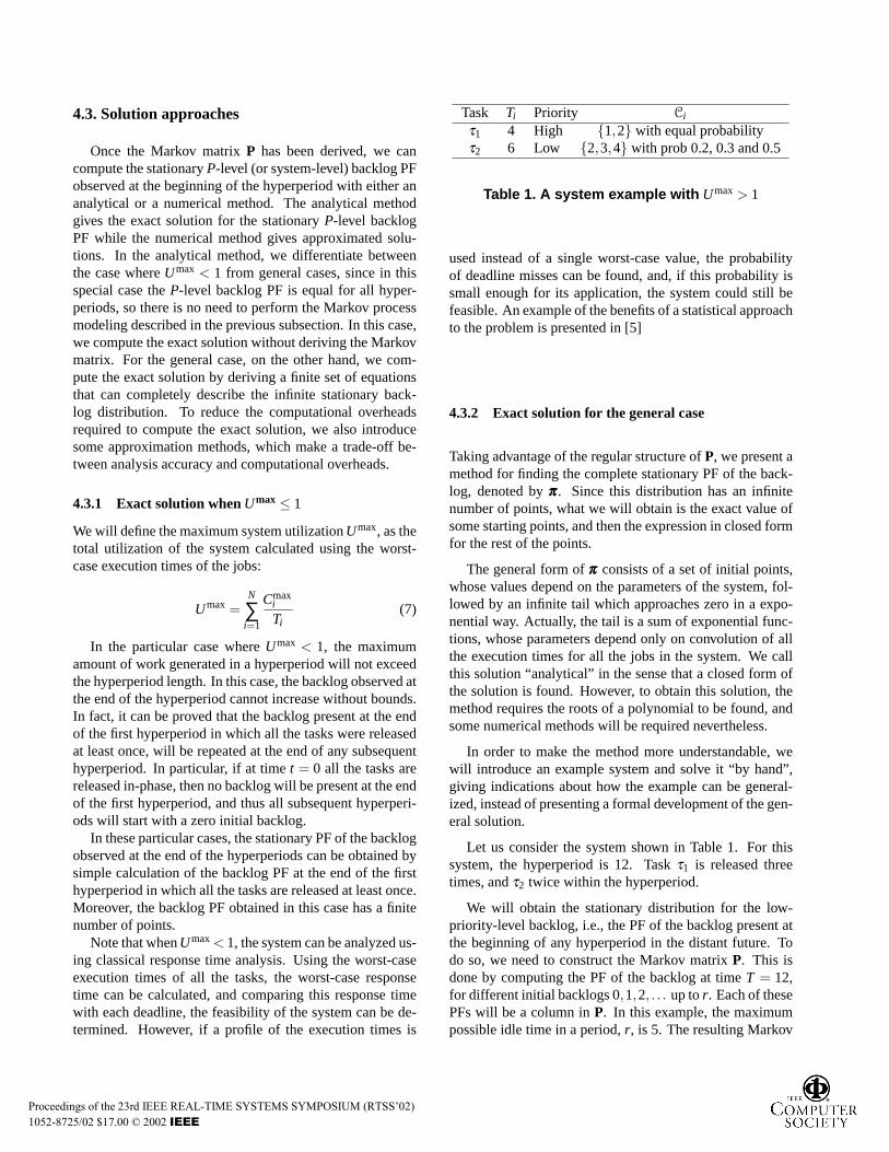
Task Ti Priority Ci

τ1 4 High {1,2} with equal probabilityτ2 6 Low {2,3,4} with prob 0.2, 0.3 and 0.5

Table 1. A system example with Umax > 1

used instead of a single worst-case value, the probabilityof deadline misses can be found, and, if this probability issmall enough for its application, the system could still befeasible. An example of the benefits of a statistical approachto the problem is presented in [5]

4.3.2 Exact solution for the general case

Taking advantage of the regular structure ofP, we present amethod for finding the complete stationary PF of the back-log, denoted byπππ. Since this distribution has an infinitenumber of points, what we will obtain is the exact value ofsome starting points, and then the expression in closed formfor the rest of the points.

The general form ofπππ consists of a set of initial points,whose values depend on the parameters of the system, fol-lowed by an infinite tail which approaches zero in a expo-nential way. Actually, the tail is a sum of exponential func-tions, whose parameters depend only on convolution of allthe execution times for all the jobs in the system. We callthis solution “analytical” in the sense that a closed form ofthe solution is found. However, to obtain this solution, themethod requires the roots of a polynomial to be found, andsome numerical methods will be required nevertheless.

In order to make the method more understandable, wewill introduce an example system and solve it “by hand”,giving indications about how the example can be general-ized, instead of presenting a formal development of the gen-eral solution.

Let us consider the system shown in Table 1. For thissystem, the hyperperiod is 12. Taskτ1 is released threetimes, andτ2 twice within the hyperperiod.

We will obtain the stationary distribution for the low-priority-level backlog, i.e., the PF of the backlog present atthe beginning of any hyperperiod in the distant future. Todo so, we need to construct the Markov matrixP. This isdone by computing the PF of the backlog at timeT = 12,for different initial backlogs 0,1,2, . . . up tor. Each of thesePFs will be a column inP. In this example, the maximumpossible idle time in a period,r, is 5. The resulting Markov

Proceedings of the 23rd IEEE REAL-TIME SYSTEMS SYMPOSIUM (RTSS’02) 1052-8725/02 $17.00 © 2002 IEEE

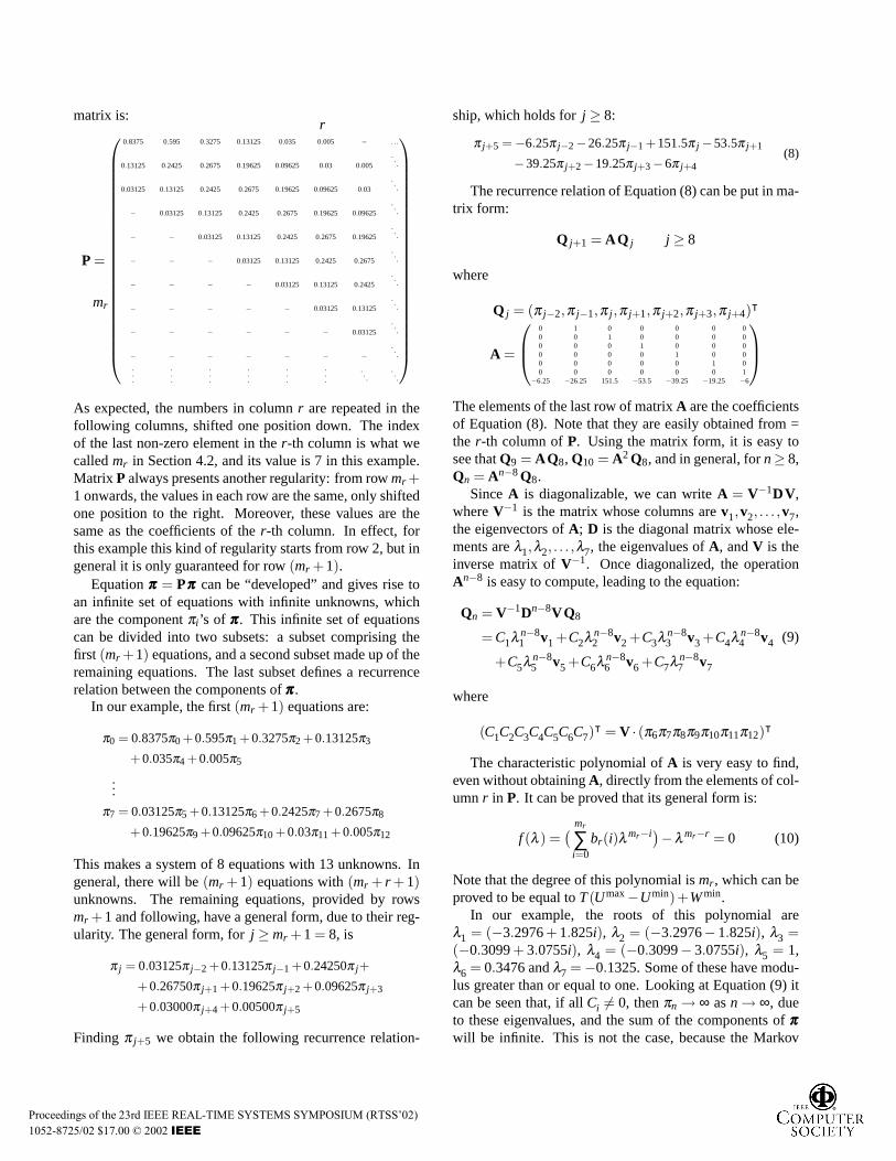
matrix is:

P =

0.8375 0.595 0.3275 0.13125 0.035 0.005 − . . .

0.13125 0.2425 0.2675 0.19625 0.09625 0.03 0.005

...

0.03125 0.13125 0.2425 0.2675 0.19625 0.09625 0.03

...

− 0.03125 0.13125 0.2425 0.2675 0.19625 0.09625

...

− − 0.03125 0.13125 0.2425 0.2675 0.19625

...

− − − 0.03125 0.13125 0.2425 0.2675

...

− − − − 0.03125 0.13125 0.2425

...

− − − − − 0.03125 0.13125

...

− − − − − − 0.03125

...

− − − − − − −...

mr

r

.

.

.

.

.

.

.

.

.

.

.

.

.

.

.

.

.

.

...

...

As expected, the numbers in columnr are repeated in thefollowing columns, shifted one position down. The indexof the last non-zero element in ther-th column is what wecalledmr in Section 4.2, and its value is 7 in this example.Matrix P always presents another regularity: from rowmr +1 onwards, the values in each row are the same, only shiftedone position to the right. Moreover, these values are thesame as the coefficients of ther-th column. In effect, forthis example this kind of regularity starts from row 2, but ingeneral it is only guaranteed for row(mr +1).

Equationπππ = Pπππ can be “developed” and gives rise toan infinite set of equations with infinite unknowns, whichare the componentπi ’s of πππ. This infinite set of equationscan be divided into two subsets: a subset comprising thefirst (mr +1) equations, and a second subset made up of theremaining equations. The last subset defines a recurrencerelation between the components ofπππ.

In our example, the first(mr +1) equations are:

π0 = 0.8375π0 +0.595π1 +0.3275π2 +0.13125π3

+0.035π4 +0.005π5

...

π7 = 0.03125π5 +0.13125π6 +0.2425π7 +0.2675π8

+0.19625π9 +0.09625π10+0.03π11+0.005π12

This makes a system of 8 equations with 13 unknowns. Ingeneral, there will be(mr +1) equations with(mr + r +1)unknowns. The remaining equations, provided by rowsmr +1 and following, have a general form, due to their reg-ularity. The general form, forj ≥mr +1 = 8, is

π j = 0.03125π j−2 +0.13125π j−1 +0.24250π j+

+0.26750π j+1 +0.19625π j+2 +0.09625π j+3

+0.03000π j+4 +0.00500π j+5

Finding π j+5 we obtain the following recurrence relation-

ship, which holds forj ≥ 8:

π j+5 =−6.25π j−2−26.25π j−1 +151.5π j −53.5π j+1

−39.25π j+2−19.25π j+3−6π j+4(8)

The recurrence relation of Equation (8) can be put in ma-trix form:

Q j+1 = AQ j j ≥ 8

where

Q j = (π j−2,π j−1,π j ,π j+1,π j+2,π j+3,π j+4)ᵀ

A =

0 1 0 0 0 0 00 0 1 0 0 0 00 0 0 1 0 0 00 0 0 0 1 0 00 0 0 0 0 1 00 0 0 0 0 0 1

−6.25 −26.25 151.5 −53.5 −39.25 −19.25 −6

The elements of the last row of matrixA are the coefficientsof Equation (8). Note that they are easily obtained from =the r-th column ofP. Using the matrix form, it is easy tosee thatQ9 = AQ8, Q10 = A2Q8, and in general, forn≥ 8,Qn = An−8Q8.

SinceA is diagonalizable, we can writeA = V−1DV,whereV−1 is the matrix whose columns arev1,v2, . . . ,v7,the eigenvectors ofA; D is the diagonal matrix whose ele-ments areλ1,λ2, . . . ,λ7, the eigenvalues ofA, andV is theinverse matrix ofV−1. Once diagonalized, the operationAn−8 is easy to compute, leading to the equation:

Qn = V−1Dn−8VQ8

= C1λn−81 v1 +C2λ

n−82 v2 +C3λ

n−83 v3 +C4λ

n−84 v4

+C5λn−85 v5 +C6λ

n−86 v6 +C7λ

n−87 v7

(9)

where

(C1C2C3C4C5C6C7)ᵀ = V · (π6π7π8π9π10π11π12)ᵀ

The characteristic polynomial ofA is very easy to find,even without obtainingA, directly from the elements of col-umnr in P. It can be proved that its general form is:

f (λ ) =( mr

∑i=0

br(i)λ mr−i)−λmr−r = 0 (10)

Note that the degree of this polynomial ismr , which can beproved to be equal toT(Umax−Umin)+Wmin.

In our example, the roots of this polynomial areλ1 = (−3.2976+ 1.825i), λ2 = (−3.2976−1.825i), λ3 =(−0.3099+ 3.0755i), λ4 = (−0.3099− 3.0755i), λ5 = 1,λ6 = 0.3476 andλ7 =−0.1325. Some of these have modu-lus greater than or equal to one. Looking at Equation (9) itcan be seen that, if allCi 6= 0, thenπn → ∞ asn→ ∞, dueto these eigenvalues, and the sum of the components ofπππ

will be infinite. This is not the case, because the Markov

Proceedings of the 23rd IEEE REAL-TIME SYSTEMS SYMPOSIUM (RTSS’02) 1052-8725/02 $17.00 © 2002 IEEE

chain is positive and thus the stationary solution has to besummable. This implies that the coefficientsC1, C2, C3, C4andC5 which multiply these eigenvalues in Equation (9),must be equal to zero. This condition gives rise to five newequations.

In general, in the case of stability, the polynomial inEquation (10) hasr roots with modulus greater than or equalto 1, and so it always providesr additional equations. Thisfact can be proved by applying Rouche’s Theorem

To summarize, we now have a linear system with 13equations, 8 from the firstmr rows of P and 5 fromthe condition of someCi ’s being zero, and 13 unknowns(π0, . . . ,π12). Nevertheless, the reader can check that theequation derived fromC5 = 0 is a linear combination ofthe others, and can be removed. In the general case, theequation derived from the eigenvalue 1, is always a linearcombination of the others. Following the described method,we will end up with a system of(mr + r) equations and(mr + r + 1) unknowns. Since the number of unknowns isone more than the number of equations, we can put each ofthe first 12 components as a linear function of the first com-ponentπ0. We will not write these expressions here for thesake of brevity. The coefficientCi ’s are also a linear func-tion of π0. In this example we obtainC6 = −0.00136π0,C7 = −1.5057·10−6 π0 (the remainingCi ’s are zero, guar-anteeing the summability ofπππ). If we use these values inEquation (9) we find the following general expression forany component ofπππ, valid for n≥ 8

Qn =−0.00136π0v6(0.3474)n−8

−1.5057·10−6π0v7(−0.1325)n−8

(11)

Note thatv6 andv7 are two eigenvectors, which were cal-culated directly from matrixA. So, the only unknown inthe above equation isπ0. For any value ofπ0, we obtain acomplete vectorπππ, which has the propertyπππ = Pπππ. How-ever, only one of these possible vectors is a PF (has a sumequal to 1). So, as a final condition, we impose∑∞

i=0 πi = 1,and from this we can determine the required value forπ0.This equation is easy to solve, despite the infinite summa-tion, because the expression forπi is a convergent sum ofexponentials, fori > 6.

Solving this sum and equating it to 1, we find the valueof π0 for this example, which isπ0 = 0.738872. From this,all the remaining values ofπππ can be computed. The first13 components are obtained directly from the system ofequations, and their values are shown in the last columnof Table 2, rounded to the sixth decimal. The remainingcomponents are calculated from the formula given in Equa-tion (11), which, after substituting the values ofπ0, v6 andv7, and taking one of the components of vectorQn, leads to:

πn = 10−4(9.4311×0.3474n−6 +0.011× (−0.1325)n−6)valid for n > 6.

B0 B1 B2 B3 B5 B10 B20 B∞0 1 0.837500 0.789734 0.768523 0.750897 0.740816 0.738968 0.7388721 − 0.131250 0.150109 0.155394 0.158160 0.158899 0.158919 0.1589172 − 0.031250 0.050976 0.059129 0.065050 0.067794 0.068186 0.0682033 − − 0.008203 0.013632 0.018639 0.021485 0.021964 0.0219874 − − 0.000977 0.002906 0.005524 0.007464 0.007850 0.0078695 − − − 0.000385 0.001372 0.002430 0.002690 0.0027056 − − − 0.000030 0.000299 0.000779 0.000934 0.0009447 − − − − 0.000053 0.000238 0.000321 0.0003288 − − − − 0.000007 0.000069 0.000110 0.0001149 − − − − 0.000000 0.000019 0.000037 0.00004010 − − − − 0.000000 0.000005 0.000013 0.00001411 − − − − − 0.000000 0.000004 0.00000512 − − − − − 0.000000 0.000001 0.000001

.

.

.

.

.

.

.

.

.

.

.

.

.

.

.

.

.

.

.

.

.

.

.

.

.

.

.

Table 2. Backlog PF convergence

4.3.3 Approximations

Truncation of matrix P One possible approximationtechnique to compute the stationary system-level backlogPF is to truncate the Markov matrixP to a sufficiently largesquare matrixP′, which was first introduced in [1]. Assum-ing that the infinite stationary distributionπππ can be modeledwith a finite vectorπππ ′ = [π ′0,π

′1,π

′2, ...,π

′n], we can lead to

the following equation fromπππ = Pπππ:

πππ′ = P′πππ ′

whereP′ is an (n+1)-by-(n+1) matrix consisting of the com-ponentP(i, j)’s (0≤ i, j ≤ n) of the Markov matrixP. Theresulting equation is an eigenvector problem, from whichwe can calculate the approximated solutionπππ ′ with a nu-merical method. Among the calculated eigenvectors, wecan choose as the approximated solution an eigenvectorwhose corresponding eigenvalue is equal to or sufficientlyclose to 1. In order to obtain a good approximation of thestationary distributionπππ, the truncation pointn should beincreased as much as possible, which makes the eigenvalueconverge to 1. Note that, by choosing an appropriate trun-cation point, we can achieve a trade-off between analysisaccuracy and the computational overheads required to solvethe corresponding eigenvector problem. The choice of aconvenient truncation point is an open issue.

Iterative approximation Another approximation tech-nique to obtain the stationary system-level backlog PF,which does not require derivation of the Markov matrixP,is the simple iteration of the algorithm which computes thePF of the backlog at the end of the hyperperiod. For the ex-ample presented in Section 4.3.2, the results of successiveiterations are shown in Table 2. It can be seen that eachpoint of the PF converges towards the analytical solution(given in the last column). It can be proved that the conver-gence is geometrically ergodic. However, it is not known inadvance how many iterations will be necessary to make thebacklog PF “close enough” to the stationary distribution. Itis clear that the rate of convergence depends on how closeUis to 1, becoming slower asU approaches 1. However, we

Proceedings of the 23rd IEEE REAL-TIME SYSTEMS SYMPOSIUM (RTSS’02) 1052-8725/02 $17.00 © 2002 IEEE

have not yet found a bound, in terms ofU , of the number ofiterations required by the iterative method.

Another important point to consider is the effect of in-troducing zero as the initial backlog for the system. In thesteady state the initial backlog is a random variable whichcan take non-zero values. Thus, the response times in thesteady state will beworsethan those calculated for the firsthyperperiod. Indeed, they will be worse than that calcu-lated for any hyperperiod. Using zero as the initial backlogwill lead to optimistic probabilities of deadline misses, sodesign decisions based on the iterative method should betaken carefully.

4.4. Extension to dynamic-priority systems

Although dynamic-priority systems seem considerablydifferent from fixed-priority systems, there exists one simi-larity. The similarity is that, in a hyperperiod, there alwaysexists at least one job that always takes the system-levelbacklogWλi, j observed at its release timeλi, j as its job-level backlogVi, j , i.e., Vi, j = Wλi, j . Such a job is calleda ground job, and has a lower priority than all the jobs re-leased before its release timeλi, j . Thus, once the stationarysystem-level backlog PFf

B0k(·) observed at the beginning

of the hyperperiod is given, the stationary job-level backlogPF fVi, j

(·) of every ground jobΓi, j can be calculated as ex-plained in Section 4.1, by iteratively applying convolutionand shrinking tof

B0k(·) for each job released between the

beginning of the hyperperiod and the release timeλi, j of thejob Γi, j (for a fixed-priority system, this statement meansthat the stationary job-level backlog PF of every job withpriority P, which is considered a ground job at the prioritylevelP, can be calculated fromf

BPk(·)).

Therefore, the difference between dynamic-priority andfixed-priority systems lies in how to compute the job-levelbacklog PFs ofnon-ground jobs. For fixed-priority sys-tems, this problem is solved by considering the higher pri-ority level that each non-ground job belongs to. Since anyjob classified as a non-ground job at a lower priority levelis bound to become a ground job at the priority level thatis equal to the priority of the job, its job-level backlog PFcan be calculated from the stationary system-level backlogPF obtained at that priority level. However, for dynamic-priority systems, we can avoid such an iterative analysis,and compute the job-level backlog PF of the non-groundjob from that of a preceding ground job. The precedingground job is the last ground job that is released before thenon-ground job and has a higher priority, which is called thebase ground jobfor the non-ground job. Since the job-levelbacklog PF of any ground job can be calculated from thesystem-level backlog PFf

B0k(·) observed at the beginning

of the hyperperiod, this means that the job-level backlogPFs of all the jobs including the non-ground jobs in the hy-

τ1

τ2

Γ1,1

0

Γ1,2

30

Γ1,3

60

Γ1,4

90

Γ1,5

120 150

Γ2,1

0

Γ2,2

50

Γ2,3

100 150

Figure 3. A task set example

Wλ1,1

Γ1,1

Wλ1,2

Γ1,2

Wλ1,3

Γ1,3

Wλ1,4

Γ1,4

Wλ1,5

Γ1,5

Wλ1,1

Γ1,1

Wλ2,1

Γ2,1

Wλ2,2

Γ2,2

Wλ2,3

Γ2,3

Wλ2,1

Γ2,1

Hyperperiod

Figure 4. Ground jobs and non-ground jobsin a dynamic-priority system

perperiod can be calculated from the system-level backlogPF f

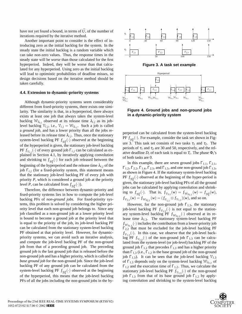
B0k(·). For example, consider the task set shown in Fig-

ure 3. This task set consists of two tasksτ1 andτ2. Theperiods ofτ1 andτ2 are 30 and 50, respectively, and the rel-ative deadlineDi of each task is equal toTi . The phaseΦi ’sof both tasks are 0.

In this example, there are seven ground jobsΓ1,1, Γ2,1,Γ1,2, Γ2,2, Γ1,4, Γ2,3, andΓ1,5, and one non-ground jobΓ1,3,as shown in Figure 4. If the stationary system-level backlogPF f

B0k(·) observed at the beginning of the hyper-period is

given, the stationary job-level backlog PFs of all the groundjobs can be calculated by applying convolution and shrink-ing to f

B0k(·). That is, fV1,1

(w) = fWλ1,1(w) = f

B0k(w),

fV2,1(w) = fWλ2,1

(w) = ( fC1,1⊗ fV1,1

)(w), and so on.

However, for the non-ground jobΓ1,3, the stationaryjob-level backlog PFfV1,3

(·) is not equal to the station-ary system-level backlog PFfWλ1,3

(·) observed at its re-lease timeλ1,3. The stationary system-level backlog PFfWλ1,3

(·) includes the contribution from a lower-priority jobΓ2,2 that must be excluded for the job-level backlog PFfV1,3

(·). In this case, we observe that the job-level back-log PF fV1,3

(·) of the non-ground jobΓ1,3 can be calcu-lated from the system-level (or job-level) backlog PF of theground jobΓ1,2 that precedesΓ1,3 and has a higher prioritythanΓ1,3 (i.e.,Γ1,2 is the base ground job of the non-groundjob Γ1,3). It can be seen that the job-level backlogV1,3

of Γ1,3 depends only on the system-level backlogWλ1,2 ofΓ1,2 and the execution time ofΓ1,2. Thus, we calculate thestationary job-level backlog PFfV1,3

(·) of the non-groundjob Γ1,3 from that of its base ground jobΓ1,2 by apply-ing convolution and shrinking to the system-level backlog

Proceedings of the 23rd IEEE REAL-TIME SYSTEMS SYMPOSIUM (RTSS’02) 1052-8725/02 $17.00 © 2002 IEEE

PF fWλ1,2(·) of the base ground jobΓ1,2 while ignoring the

lower-priority ground jobΓ2,2. This approach can be gener-alized to compute the stationary job-level backlog PF of anarbitrary non-ground jobΓi, j as follows.

Theorem 1. For any non-ground jobΓi, j , the stationaryjob-level backlog PF fVi, j

(·) can be computed from the sta-tionary system-level backlog PF fWλk,l

(·) of its base groundjob, (i.e., the last ground jobΓk,l that precedesΓi, j and hasa priority higher than that ofΓi, j ) by iteratively applyingconvolution and shrinking to fWλk,l

(·) only for all the non-ground jobs that are released in the time interval (λk,l , λi, j ]and have priorities higher than that ofΓi, j . �

Note that, in a system scheduled by EDF, we can findthe base ground job for any non-ground job, since there al-ways exists a ground job that has an earlier deadline thanthe non-ground job. For a general dynamic-priority sys-tem, we developed a systematic approach to finding the baseground job for any non-ground job and computed the job-level backlog PF of the non-ground job in a systematic way,but we do not include it here for the sake of brevity. Formore information, refer to [8].

5. Experimental results

In this section, we give experimental results obtained bythe proposed stochastic analysis. First, we compare the re-sults obtained from the proposed analysis method (both theexact solution and the approximated solution based on theMarkov matrix truncation) with those obtained by Stochas-tic Time Demand Analysis (STDA) [7, 6] using the exam-ple given in [6]. Secondly, we compare the results obtainedusing the truncation method with those obtained from simu-lations while varying the average system utilization and thenumber of tasks.

5.1. Comparison with STDA

To compare the proposed analysis method with STDA,we used the same task sets given in [6], which are shownin Table 3. All three task sets in Table 3 are assumed tobe scheduled by RM and have the same task parameters ex-cept for the execution time PFs of tasks given by a uniformPF that ranges fromCmin

i to Cmaxi (Cmax

i = 2× Ci −Cmini )

for taskτi . For the task sets, the simulation results and theanalytical results given by STDA are copied from [6] andcompared with the results given by the proposed stochas-tic analysis, using the exact solution and the approximationobtained by the Markov matrix truncation. The results inTable 4 show that there is a significant difference betweenthe deadline miss probability given by STDA and the oneobtained by the proposed method, which is almost identicalto the simulation result. This results from the critical instant

assumption made in STDA. The negative impact on thedegradation of analysis accuracy increases with an increasein the (maximum) system utilization. In the case of taskτ2in S2, the deadline miss probability given by STDA is morethan six times the one given by the proposed method.

S τi Ti Di Cmini Ci Cmax

i U Umax

S1τ1 300 300 72 100 128

0.708 0.997τ2 400 400 72 150 228

S2τ1 300 300 50 100 150

0.708 1.125τ2 400 400 50 150 250

S3τ1 300 300 1 100 199

0.708 1.411τ2 400 400 1 150 299

Table 3. Task sets in [6]

S τi simulation STDA Exact analysis Approximation

S1τ1 0.000± 0.000 0.000 0.000 0.000τ2 0.047± 0.001 0.141 0.047 0.047

S2τ1 0.000± 0.000 0.000 0.000 0.000τ2 0.074± 0.002 0.489 0.074 0.074

S3τ1 0.000± 0.000 0.000 0.000 0.000τ2 0.192± 0.001 0.608 0.192 0.191

Table 4. Results for the task sets in Table 3

5.2. Sensitivity to the average system utilization andthe number of tasks

To assess the sensitivity of analysis accuracy to the aver-age system utilization, we performed experiments with tasksets consisting of three and five tasks while varying the av-erage system utilization from 0.70 to 0.96. For each exper-iment, we also considered both RM and EDF scheduling toinvestigate the effect of the scheduling policy on analysisaccuracy. The results (which we do not detail here due tospace limit), showed that the approximated solutions fromthe Markov matrix truncation is almost equal to the simula-tion results for most cases. In the case of the task sets con-sisting of three tasks, the error between the approximatedsolution and the simulation result of the deadline miss prob-ability for a task ranges from 0 to 0.006 for RM, and from0 to 0.008 for EDF. In the case of the task sets consistingof five tasks, the error ranges from 0 to 0.015 for RM, andfrom 0 to 0.028 for EDF. According to the results, the errorincreases as the average system utilization increases. Forexample, in the case where the task set consisting of fivetasks are scheduled by EDF, the error was 0, 0.002, 0.016,0.028 when the average system utilization was 0.7, 0.8, 0.9,0.96, respectively. The inaccuracy is due to the Markov ma-trix truncation, which converts the Markov matrix with aninfinite dimension to one with a finite dimension. When thestationary system-level backlog PF we are trying to obtainhas a non-negligible tail distribution beyond the truncationpoint, the Markov matrix truncation inevitably introducesapproximation errors in the analysis. To reduce these er-rors, it is necessary to preserve the tail distribution as much

Proceedings of the 23rd IEEE REAL-TIME SYSTEMS SYMPOSIUM (RTSS’02) 1052-8725/02 $17.00 © 2002 IEEE

as possible by choosing a larger truncation point at the costof greater computational overheads. For more information,the reader is referred to [8].

6. Conclusions and future work

In this paper we have introduced a model and a concep-tual framework which allows statistical analysis of the re-sponse time of periodic tasks in a general priority-drivenreal-time system. The model requiresa priori knowledgeof the probability function (PF) of the execution time re-quired by each job. We have derived formulae for calcu-lating the backlog PF at any time, and the response timePF of any task. The statistical information derived from theanalysis can be combined with deadlines, thus obtaining theprobability of deadline misses for any task in the system. Ifthis probability is zero for a task, then its deadline is guar-anteed. In this sense the statistical analysis subsumes theclassical response-time analysis. The analysis also allowsfor systems withUmax> 1, which would not be feasible us-ing classical analysis. WheneverU < 1, the long-term sta-tistical behavior can be described by modeling the backlogprocess as a Markov chain.

The model still has some limitations which can beinvestigated. It does not allow for uncertainty in the releasetimes of the jobs, and assumes all tasks to be independent,so it does not allow for blocking in shared resources.Furthermore, the assumed independence is also statistical,i.e. the execution time distribution of a task is assumed tobe independent of the values observed for the other tasks, orfor previous instances of the same task. This assumption isoften violated in real-world cases. When the number of jobsin a hyperperiod is large, finding the stationary distributionanalytically is too expensive (although possible), so somenumerical methods have been provided as approximations.In future work, the error introduced for such methodsshould be studied, and the development of a numericalmethod that can bound the error is needed.

AcknowledgementThe authors of this paper arepleased to thank Prof. Guillem Bernat and Prof. Jane Liu aswell as the anonymous reviewers for the valuable commentsand observations they provided.

References

[1] L. Abeni and G. Buttazzo. Stochastic Analysis of a Reserva-tion Based System. InProc. of the 9th International Work-shop on Parallel and Distributed Real-Time Systems, Apr.2001.

[2] A. K. Atlas and A. Bestavros. Statistical Rate MonotonicScheduling. InProc. of the 19th IEEE Real-Time SystemsSymposium, pages 123–132, Dec. 1998.

[3] G. Bernat, A. Colin, and S. Petters. WCET Analysis of Prob-abilistic Hard Real-Time Systems. InProc. of the 23rd IEEEReal-Time Systems Symposium, Dec. 2002.

[4] A. Burns. Preemptive Priority Based Scheduling: An Ap-propriate Engineering Approach. In S. H. Son, editor,Ad-vances in Real-Time Systems. Prentice Hall, 1994.

[5] J. L. Dıaz, J. M. Lopez, and D. F. Garcıa. Prob-abilistic Analysis of the Response Time in a Real-Time System. InProc. of the 1st CARTS Workshopon Advanced Real-Time Technologies, Aranjuez, Spain,Oct. 2002. Also available as Technical Report athttp://www.atc.uniovi.es/research/PART01.pdf.

[6] M. K. Gardner. Probabilistic Analysis and Scheduling ofCritical Soft Real-Time Systems. PhD thesis, University ofIllinois, Urbana-Champaign, 1999.

[7] M. K. Gardner and J. W. Liu. Analyzing Stochastic Fixed-Priority Real-Time Systems. InProc. of the 5th Interna-tional Conference on Tools and Algorithms for the Construc-tion and Analysis of Systems, Mar. 1999.

[8] K. Kim, L. L. Bello, C.-G. Lee, S. L. Min, and O. Mirabella.An Accurate Stochastic Analysis of General Priority-DrivenReal-Time Systems. Technical report, School of ComputerScience and Engineering, Seoul National University, 2002.Also available at http://archi.snu.ac.kr/khkim/sapds02.ps.

[9] K. Kim, L. L. Bello, S. L. Min, and O. Mirabella. On Re-laxing Task Isolation in Overrun Handling to Provide Prob-abilistic Guarantees to Soft Real-Time Tasks with VaryingExecution Times. InProc. of the 14th Euromicro Confer-ence on Real-Time Systems, Jun. 2002.

[10] L. Kleinrock. Queueing Systems. John Wiley & Sons, 1975.[11] J. P. Lehoczky. Fixed Priority Scheduling of Periodic Task

Sets with Arbitrary Deadlines. InProc. of the 11th IEEEReal-Time Systems Symposium, pages 201–209, Dec. 1990.

[12] J. P. Lehoczky. Real-Time Queueing Theory. InProc. of the17th IEEE Real-Time Systems Symposium, pages 186–195,Dec. 1996.

[13] J. P. Lehoczky. Real-Time Queueing Network Theory.In Proc. of the 18th IEEE Real-Time Systems Symposium,pages 58–67, Dec. 1997.

[14] J. P. Lehoczky, L. Sha, and Y. Ding. The Rate-MonotonicScheduling Algorithm: Exact Characterization and AverageCase Behavior. InProc. of the 10th IEEE Real-Time SystemsSymposium, Dec. 1989.

[15] J. Leung and J. Whitehead. On the Complexity of Fixed Pri-ority Scheduling of Periodic Real-Time Tasks.PerformanceEvaluation, 2(4):237–250, 1982.

[16] L. Liu and J. Layland. Scheduling Algorithms for Multi-programming in a Hard Real-Time Environment.Journal ofACM, 20(1):46–61, 1973.

[17] A. K. Mok and D. Chen. A Multiframe Model for Real-Time Tasks. IEEE Transactions on Software Engineering,23(10):635–645, Oct. 1997.

[18] T.-S. Tia, Z. Deng, M. Shankar, M. Storch, J. Sun, L.-C.Wu, and J.-S. Liu. Probabilistic Performance Guarantee forReal-Time Tasks with Varying Computation Times. InProc.of the Real-Time Technology and Applications Symposium,pages 164–173, Chicago, Illinois, May 1995.

[19] K. Tindell, A. Burns, and A. J. Wellings. An Extendible Ap-proach for Analyzing Fixed Priority Hard Real-Time Tasks.Real-Time Systems, 6:133–151, 1994.

Proceedings of the 23rd IEEE REAL-TIME SYSTEMS SYMPOSIUM (RTSS’02) 1052-8725/02 $17.00 © 2002 IEEE