Stephen Quinn, Texas Christian University William Roberds ...

45

Supplementary material for

How Amsterdam got Fiat Money

Stephen Quinn, Texas Christian University

William Roberds, Federal Reserve Bank of Atlanta

46

Appendix A: AWB Accounting

I. The Balance Sheet

The AWB fiscal year ended of January, so the bank’s balance sheet sums categories on

January 31. In bank guilders, the AWB reported its assets as metal held and loans due, its liabili-

ties were account balances, and the residual was capital. See Table 1 in the text for an example.

Van Dillen (1925: 701-807) reproduces these from AWB records, and we have consolidated

them for our sample period in Table A1.

Because the balance sheet is a double entry system, changes in year-to-year balances have

an offsetting change, so bank operations can be organized within a matrix. Figure A1 shows the

possibilities and assigns different AWB operations to the appropriate categories. Traditional de-

posits and withdrawals are only the start. In particular, credit activity follows from changes in

metal levels or account levels without an offsetting change in the other. Put differently, metal

derives from activity in the other two categories: capital and loans.

Figure A1. Cross-Category AWB Operations

Metal Loans Capital Account Deposits

Withdrawals Bullion purchases and sales

“Account” Lending: All VOC, Some Amsterdam

VOC Interest Some Expenses

Capital Fee Revenue Holland Interest Most Expenses Special Deposits Open Market Profit/Loss

Interest Due Loan Write-Offs

Loans “Metal” Lending: All Holland, All Miscellaneous, Some Amsterdam

Loans

Loans were granted by creating account balances (VOC) or by releasing metal (Holland).

Amsterdam used both techniques. Principal repayment reversed the process.

Capital Accumulation

Capital grew through the bank’s retained earnings. Interest payments by account eliminated

bank guilders while interest payments by metal increased the bank’s metal stock. If the bank

47

considered interest due on January 31, then the AWB added the interest due to the loan’s princi-

pal and to the bank’s capital at that time. Other revenue from fees on withdrawals, account over-

drafts, receipts and money changing were collected in coin, so the metal stock increased from

those operations.

Capital Extraction

Removing capital was the prerogative of the City of Amsterdam. When the city decided to

extract retained earnings, it did so by “borrowing” from the AWB at no interest instead of reduc-

ing capital. It appears the city did this to avoid explicitly putting the AWB into a negative capi-

tal. This situation seems to have evolved. In the early 1650s, the city borrowed around 2 million

guilders from the AWB to help build a new city hall (and home for the bank) on the Dam. Soon,

the city stopped paying interest, for why pay your own bank (van Dillen?)? Beginning in 1685,

when retained earnings had built sufficient capital, the city had the AWB write off both capital

and some of the bank’s outstanding loans to the city until the AWB’s book capital was again

near zero, but not negative.

We agree with Willemsen (2009) that the city’s taking of metal and creating of balances

should be treated as capital extraction rather than as loans. To see the consequences of this inter-

pretation, we calculate adjusted values for capital, loans, and assets. Adjusted capital subtracts

the money from capital when the operation occurred instead of when the AWB later wrote-off

the loan. Adjusted loans do not add the city as a borrower and do not subsequently write down

those loans. Adjusted assets use the adjusted loans series: metal stock plus adjusted loans. Figure

A2 compares book and adjusted capital-to-asset ratios. Figure A3 compares book and adjusted

loans-to-asset ratios. The adjusted loan-to-asset ratio is sometimes lower than book because mu-

nicipal loans are ignored but sometimes higher than book because write-offs are also ignored.

Table A2 reports the adjusted values.

48

Figure A2. AWB Capital-to-Asset Ratios, 1610 to 1795

Source: Derived by authors from van Dillen (1925, 701-807).

Figure A3. AWB Loan-to-Asset Ratios, 1610 to 1795

Source: Derived by authors from van Dillen (1925, 701-807).

49

The AWB balance sheet, however, does not communicate two important categories of informa-

tion: gross flows and intra-category activity. The next sections report our efforts to reconstruct

gross flows between bank accounts and the other balance sheet categories (see Figure A1).

II. The Specie Kamer

To account for the creation and destruction of bank guilders, the AWB used a master ac-

count called the Specie Kamer (or Kammer or Camer) that translates as specie room. Specie

Kamer transactions are the top row of Figure A1: deposits and withdrawals (account-metal),

VOC and some Amsterdam loans (account-loan), VOC interest payments and some AWB ex-

pense payments (account-capital). The bulk of this paper’s evidential contribution has involved

using the Specie Kamer to reconstruct these transactions. This section details how we did this

and what we found.

The Bank of Amsterdam organized its books by half-year increments: February through

July, August through January. By the 1700s, the bank needed 3,000 pages to record each half-

year of bank activity. The amount of information in the ledgers is staggering. Fortunately for our

purposes, the Specie Kamer master accounts are only a few pages per ledger.

Receivers

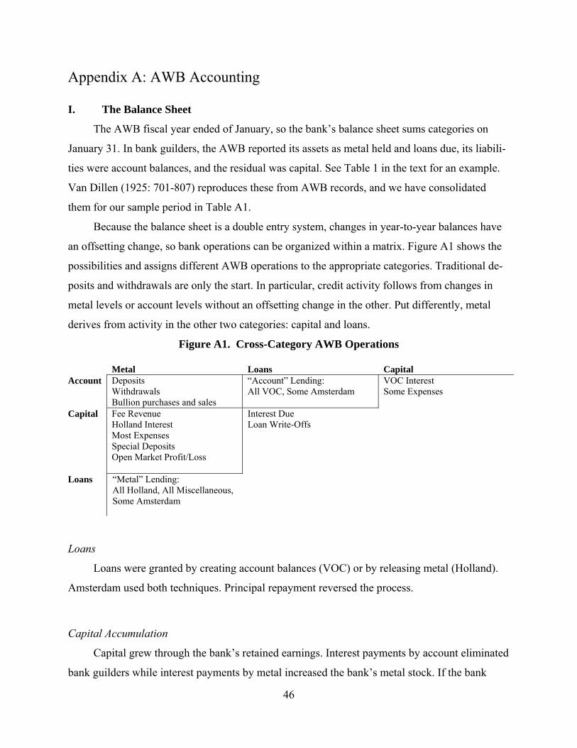
The bank used two sets of accounts to represent itself. When customers brought a deposit

to the bank, the bank usually debited an account in the name of the employee who received the

metal. Most years, the bank had two or three such receivers, and this system began in the 1620s.

When metal left, the Bank of Amsterdam credited the Specie Kamer. As a result, the combina-

tion of receiver debits and the specie room credits gives the changes in the amount of bank

money. Figure A4 offers a schematic of the flow of metal and bank money through the bank.

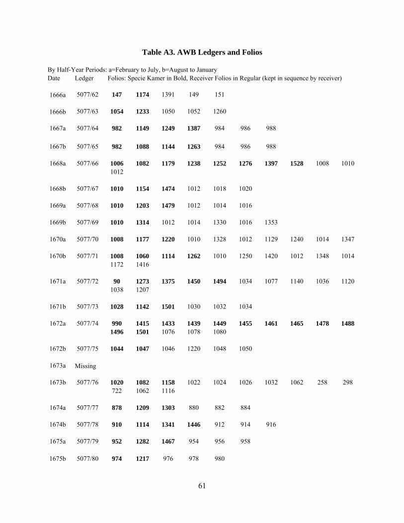
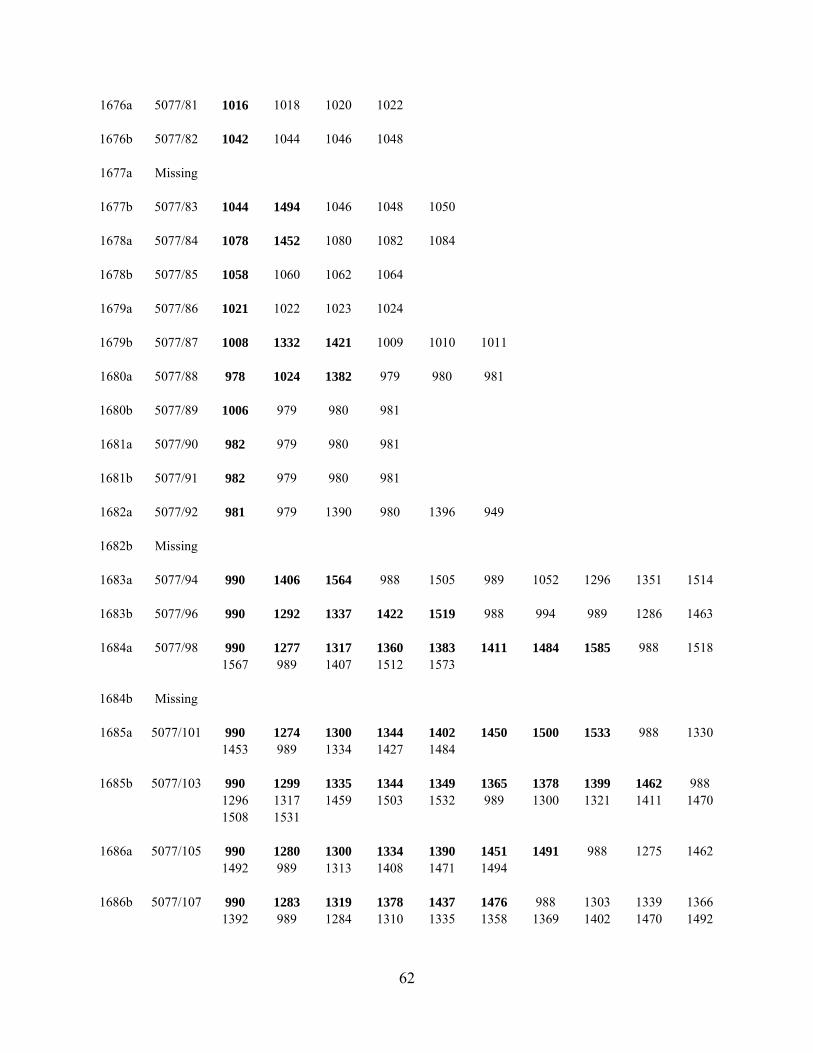
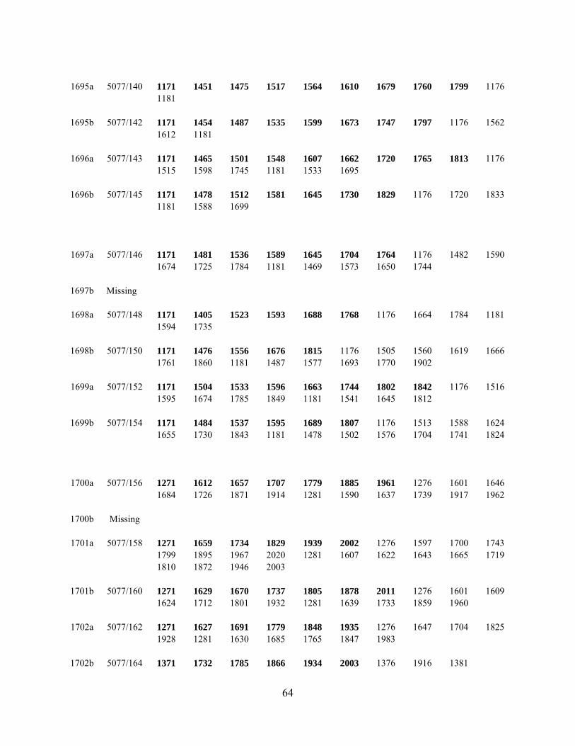
Table A3 lists the 74 ledgers and 812 folios used in this study. All ledgers are stored at the Am-

sterdam Municipal Archives, and the archive retains dissemination rights over the images. The

folios were digitally photographed and then encoded.

50

Figure A4. Standard Metal Flow through the Bank of Amsterdam

Here is an example of how the deposit process worked. On 23 May 1687, Arthur Woodward

received metal worth 480 bank guilders from Samuel Cohen (5077/109, f.1407). Cohen’s ac-

count was credited and Woodward’s account was debited. The ledger does not report what

Cohen deposited, but it was likely a sack (a standard unit for bulk coins) of 200 silver Dukaat

coins at 2.4 guilders each. If so, then Cohen also should have received a receipt granting the op-

tion to buy 200 Dukaats from the AWB for 480 bank guilders. We say should because the ac-

count ledgers never mention receipts. Two weeks later, on June 6, Woodward transferred 46,800

guilders in metal to the Specie Kamer: Woodward’s account was credited (5077/109, f. 1445)

and the Specie Kamer debited (5077/109, f. 1431).

Non-Metallic Guilder Creation

Some guilder creation, however, did not involve incoming metal, and the AWB recorded

these directly in the Specie Kamer account and bypassing the receivers. For example, when the

VOC borrowed money from the AWB, the VOC’s account was credited and the Specie Kamer

was debited. To create our borrowing and repayment series, we separate account loans from de-

posits and repayments from withdrawals.

Bank of Amsterdam

Metal Metal

Deposit Customer

Withdrawal Customer

Bank Bank Money Money

Bank Receiver

Specie Kamer

51

For some years, extant AWB records tell exact loan creation, repayment and interest pay-

ments (AMA 5077/1311 through 1323), so we found the matching transactions. For other years,

van Dillen (1925, 979-84) provides total VOC borrowing, repayment and interest, so the match-

ing transactions can be readily found, for the transactions were labeled VOC, and borrowing

occurred in 100,000 guilder increments, with the rare exception of a 50,000 increment. Repay-

ments are similarly named and carry the correct amounts for interest.

For the remaining years (1671 through 1675 and 1683 through 1684), the challenge is ac-

counting for loans when we have only year start and year end debt levels. For these years, we

have looked for 1) large, round VOC debits and 2) offsetting VOC credits that include the cor-

rect interest that 3) combine to leave the correct debt outstanding. Table A4 reports the loans we

have identified. The interest rate was a consistent 4 percent except for anticipations in the mid-

1670s (de Korte 1984, 66), and the internal rates of return reflect that rate. Finally, we note that

the ledger for August 1684 to January 1685 is missing and detailed summaries are missing, so

we know nothing about that period except that 400,000 guilders in principal was retired.

Occasionally, the City of Amsterdam also created accounts without depositing metal. As

with the VOC, the AWB credited the City of Amsterdam by debiting the Specie Kamer. These

transactions are detailed in the bank’s balance book records (AMA 5077/1311 through 1323), so

we can separate them from metal transactions. Table A5 lists the municipal transactions that

changed the supply of guilder (account transactions). Table A5 also lists when the city moved

metal in or out of the bank but did not change the guilder money supply (metal transactions).

Combining these two transaction types gives the full accounting of the city’s extraction of capital

from the bank.

Bullion

After removing 1) loans and 2) transfers from receivers, the debit side of the Specie Kamer

still contains some direct deposits that avoid the receivers. We lack a contemporaneous descrip-

tion of why some deposits were processed through receivers while others were not, but we think

that bullion was directly deposited into the Specie Kamer while coins went through the receivers.

To begin, the use of receiver accounting begins in the 1620s, so the distinction predates receipts

or the agio. Next, the direct deposits are far more likely to involve a remainder less than a guil-

der, and even less than a stuiver (1/20th of a guilder). In contrast, receivers see far more large

52

round deposits. Table A6 measures this dramatic difference through the percent of deposit trans-

actions by depository channel that fall into large round values or into odd values. Bullion tends

towards odd values because it is valued by weight and fineness, so a piece of bullion would

rarely hit exactly a round guilder value. In contrast, official coins carried assigned values de-

nominated in stuivers: 0.05 guilder increments and almost all in 0.1 increments (Menno S. Polak,

Historiografie en Economie van de “Muntchaos,” De Muntproductie van de Republiek 1606-

1795, Deel I (1998), NEHA, Amsterdam, pp. 67-101). The standard bulk unit for coins was a

sack of 200, so round guilder values are common. Multiple sacks produce large values round to

100 guilders or even 1,000 guilders.

In practice, the difference looks like this. On July 20, 1688, Samuel Cohen made two de-

posits that were both credited to the same account (5077/113 f. 1491). With the receiver Arthur

Woodward, Cohen deposited 2,400 guilders that could easily have been 4 sacks of silver rijders

(a standard trade coin) at the ordinance value of 3 guilders per coin (5077/113 f. 1517). Through

the Specie Kamer, Cohen deposited 6,873.25 guilders (5077/113 f. 1484). That sum is difficult to

reach using standard coins if for no other reason than almost all Dutch coins were priced in even

stuivers (0.1 increments). More importantly, we think the bullion-coin divide explains why

Cohen made two deposits on the same day, for the pattern can be found on other days. For ex-

ample, six days earlier, Cohen had deposited 11,073.075 guilders in the Specie Kamer and 3,675

guilders through a receiver (5077/131, ff. 1484, 1517).

Our interpretation has other support. In April and May 1668, the Specie Kamer debits

surged, and our theory suggests that this is a period of open market purchases. The AWB’s mint

orders survive for that year, and simultaneous with the purchases, the bank sent large quantities

of silver bullion (480,003 guilders worth) to the various mints from 27 April to 30 May

(5077/1313). Table A7 reports the guilder value sent to each mint.

Unfortunately for our purposes, the AWB did not separate metal outflows into different ac-

counts, so we use odd values as a proxy for bullion. While not perfect, a sort by odd-value versus

round-value seems to reasonably mirror long-term behavior on the deposit side as seen in Figures

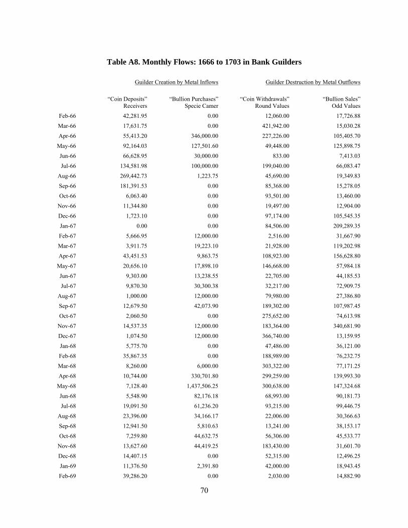
X and Y. Also, we know that the great run of June 1672 was not an open market operation. In

that month, round values withdrawals (our proxy for coin) totaled 2.5 million guilders while odd-

values withdrawals (our proxy for bullion) totaled 0.3 million guilders. The monthly flow of

these series is reported in Table A8.

53

III. Fee Ratios

Having reconstructed withdrawals for our sample period, we calculated an average fee per

year by dividing fee revenue by total withdrawals. Table A9 reports the numbers in ratio of fee

revenue over metal outflows.

Fee revenue had to be constructed for the years 1666 to 1684, for the AWB reported total

revenue. We adjusted revenue for the AWB’s practice of counting interest due from the VOC as

revenue and subsequently not counting the actual interest payments. Next we removed interest

payments from the VOC (by Specie Kamer account) and from the Province of Holland (by

metal) to get a remainder to proxy “withdrawal fee” revenue. The proxy overstates actual with-

drawal fee revenue, for it also includes other minor fees like overdraft charges. We do not report

revenue for the fiscal year 1673 because the bank replaced its regular revenue and expenses with

a single 67,247 write down caused by the re-pricing of Russian coins held by the bank (van Dil-

len 1925: 746). 1677, 1682 and 1684 lack complete withdrawal information because of missing

ledgers. The 1679 withdrawal numbers are low (fee ratio high) because we lack one Specie

Kamer folio for that year.

1683 is the only year during the receipt regime for which we have revenue and withdraw-

als. The ratio is 0.67 percent, but it is a poor proxy for withdrawal fees. Under the new regime,

one paid a receipt fee to rollover the option, so no metal need leave the bank. Also the bank be-

gan charging a transfer fee of 0.025 percent (van Dillen 1934: 84). We cannot separate these

different revenue sources, so we can only state that fee revenue dropped to a low rate in the year

receipts were adopted.

IV. VOC

Table A10 considers the AWB as a creditor to the VOC in two ways: levels and flows.

Column 1 reports the amount the VOC owed to the AWB in bank guilders. We calculate this

amount using the bank’s records. The VOC records do not identify creditors. Column 2 reports

the level of the VOC’s total debt in current guilders. The total debt is comprised of obligations of

the company in general, obligations of each chamber, anticipations, bills of exchange, and mis-

54

cellaneous creditors. Column 3 gives the AWB’s share of the total and assumes an agio of 4.5

percent.

While some years find the VOC owing 10 to 20 percent of its debt to the AWB, 15 out of

36 fiscal years closed with the company owing nothing to the bank. Levels suggest that in the

VOC relied on the AWB as a substantial multi-year lender in and near the 1680s. Otherwise, the

AWB was a long-term lender of little consequence.

To see the short-term credit story, we have reconstructed the amount the VOC borrowed

from the AWB during each fiscal year (column 4). We do not report repayment, for we already

know that often this debt was repaid within the year. Instead, we wonder how the VOC was us-

ing the AWB to facilitate operations during a fiscal year. Unfortunately, the VOC records do not

tell us intra-year borrowing, so we cannot calculate the AWB’s share of all short-term lending to

the VOC.

We do know, however, some general measures of VOC activity, so we instead see what

correlates with VOC borrowing from the AWB. Our approach is descriptive and seeks only the

gentlest of inferences regarding why the VOC borrowed from the AWB. As a dependent vari-

able, we have the amount of VOC borrowing from the AWB per fiscal year in bank guilders. For

explanatory variables, we know the following in current guilders:

Two activities potentially creating demand for loans:

1. The total amount spent by the VOC in the Netherlands outfitting ships, paying in-

terest, etc.

2. The amount of cash dividends paid out by the company to shareholders.

One activity potentially reducing the demand for loans

3. The total amount collected by the VOC from selling goods.

And a few VOC balance sheet items (levels) at the start of each fiscal year that might af-

fect demand for AWB loans in the forthcoming year:

4. The trade good inventory

5. The cash and bank balances

6. Trade credits due to the VOC

7. The total external debt

55

We regressed AWB lending on these seven variables using OLS with no modifications, and

the result is in the paper as Table X. Expenditures strongly and positively correlate with borrow-

ing. They suggest a derived demand for AWB loans of 25 percent of total expenditures. In con-

trast, Information about that year’s sales revenue lacks any explanatory power. These results

agree with the idea that the VOC was borrowing to outfit ships before the year’s fleet returned

from Asia.

Dividends appear of occasional consequence, and we cannot sort out why some dividends

correlate with AWB borrowing while others do not.

Of the four start-of-year levels, the three assets (substitutes to AWB loans) do have nega-

tive coefficients. While not statistically significant, the inventor and credit due levels suggest

notable effects. Starting cash appears of little import. Finally, the level of VOC debt at the start

of a fiscal year gives little information regarding AWB loans.

In total, we feel that comparing AWB loan amounts to yearly VOC expenditures (Column

5) gets at the heart of the AWB-VOC credit relationship. While that share (Column 6) did vary,

AWB loans became a routine, and often substantial, part of financing yearly ship outfitting.

V. Interpolation of the agio

The agio series was interpolated using a time series on the London price of a bill of ex-

change payable in Amsterdam (McCusker 1978, Table 2.8), quoted as bank schillings (i.e., 0.3

guilders) per pound sterling. The bill price series contains 179 monthly observations over the

sample period, including 77 months for which there is no corresponding agio observation. A

Kalman filter routine was used to fit a 3-month, bivariate VAR by maximum likelihood to all

available observations on the agio and on the bill price. Interpolated values of the agio are the

values returned by the Kalman smoother at the ML estimates.

The accuracy of this method was tested by simulations, in which a random selection of agio

observations (excluding the 1672 and 1693 outlier periods) were removed from the sample and

then estimated using the interpolation procedure described above. The standard error of the

smoothed estimates of the agio ranges from about 22 basis points over the holdout sample (with

a 5 percent probability of observations being allocated to holdout sample) to 35 basis points

56

(with a 50 percent probability). These are smaller than sample standard deviation of the agio

series (about 50 basis points; see Table 3), suggesting that the interpolation procedure is of value

in estimating missing values of the agio.

57

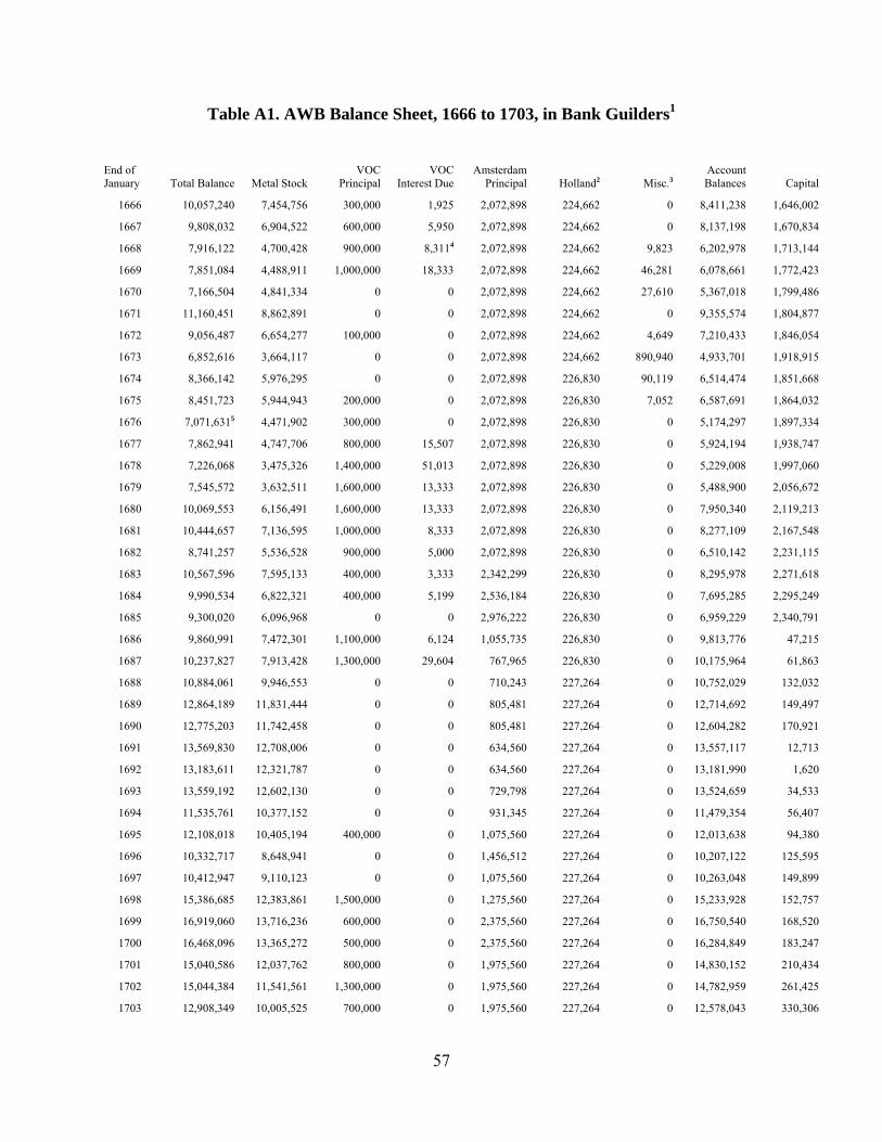
Table A1. AWB Balance Sheet, 1666 to 1703, in Bank Guilders1

End of January Total Balance Metal Stock

VOC Principal

VOC Interest Due

Amsterdam Principal Holland2 Misc.3

Account Balances Capital

1666 10,057,240 7,454,756 300,000 1,925 2,072,898 224,662 0 8,411,238 1,646,002

1667 9,808,032 6,904,522 600,000 5,950 2,072,898 224,662 0 8,137,198 1,670,834

1668 7,916,122 4,700,428 900,000 8,3114 2,072,898 224,662 9,823 6,202,978 1,713,144

1669 7,851,084 4,488,911 1,000,000 18,333 2,072,898 224,662 46,281 6,078,661 1,772,423

1670 7,166,504 4,841,334 0 0 2,072,898 224,662 27,610 5,367,018 1,799,486

1671 11,160,451 8,862,891 0 0 2,072,898 224,662 0 9,355,574 1,804,877

1672 9,056,487 6,654,277 100,000 0 2,072,898 224,662 4,649 7,210,433 1,846,054

1673 6,852,616 3,664,117 0 0 2,072,898 224,662 890,940 4,933,701 1,918,915

1674 8,366,142 5,976,295 0 0 2,072,898 226,830 90,119 6,514,474 1,851,668

1675 8,451,723 5,944,943 200,000 0 2,072,898 226,830 7,052 6,587,691 1,864,032

1676 7,071,6315 4,471,902 300,000 0 2,072,898 226,830 0 5,174,297 1,897,334

1677 7,862,941 4,747,706 800,000 15,507 2,072,898 226,830 0 5,924,194 1,938,747

1678 7,226,068 3,475,326 1,400,000 51,013 2,072,898 226,830 0 5,229,008 1,997,060

1679 7,545,572 3,632,511 1,600,000 13,333 2,072,898 226,830 0 5,488,900 2,056,672

1680 10,069,553 6,156,491 1,600,000 13,333 2,072,898 226,830 0 7,950,340 2,119,213

1681 10,444,657 7,136,595 1,000,000 8,333 2,072,898 226,830 0 8,277,109 2,167,548

1682 8,741,257 5,536,528 900,000 5,000 2,072,898 226,830 0 6,510,142 2,231,115

1683 10,567,596 7,595,133 400,000 3,333 2,342,299 226,830 0 8,295,978 2,271,618

1684 9,990,534 6,822,321 400,000 5,199 2,536,184 226,830 0 7,695,285 2,295,249

1685 9,300,020 6,096,968 0 0 2,976,222 226,830 0 6,959,229 2,340,791

1686 9,860,991 7,472,301 1,100,000 6,124 1,055,735 226,830 0 9,813,776 47,215

1687 10,237,827 7,913,428 1,300,000 29,604 767,965 226,830 0 10,175,964 61,863

1688 10,884,061 9,946,553 0 0 710,243 227,264 0 10,752,029 132,032

1689 12,864,189 11,831,444 0 0 805,481 227,264 0 12,714,692 149,497

1690 12,775,203 11,742,458 0 0 805,481 227,264 0 12,604,282 170,921

1691 13,569,830 12,708,006 0 0 634,560 227,264 0 13,557,117 12,713

1692 13,183,611 12,321,787 0 0 634,560 227,264 0 13,181,990 1,620

1693 13,559,192 12,602,130 0 0 729,798 227,264 0 13,524,659 34,533

1694 11,535,761 10,377,152 0 0 931,345 227,264 0 11,479,354 56,407

1695 12,108,018 10,405,194 400,000 0 1,075,560 227,264 0 12,013,638 94,380

1696 10,332,717 8,648,941 0 0 1,456,512 227,264 0 10,207,122 125,595

1697 10,412,947 9,110,123 0 0 1,075,560 227,264 0 10,263,048 149,899

1698 15,386,685 12,383,861 1,500,000 0 1,275,560 227,264 0 15,233,928 152,757

1699 16,919,060 13,716,236 600,000 0 2,375,560 227,264 0 16,750,540 168,520

1700 16,468,096 13,365,272 500,000 0 2,375,560 227,264 0 16,284,849 183,247

1701 15,040,586 12,037,762 800,000 0 1,975,560 227,264 0 14,830,152 210,434

1702 15,044,384 11,541,561 1,300,000 0 1,975,560 227,264 0 14,782,959 261,425

1703 12,908,349 10,005,525 700,000 0 1,975,560 227,264 0 12,578,043 330,306

58

Source is authors’ adjustment of van Dillen (1925, 741-762) Notes for Table A1:

1. Holland’s debt is in current guilders. 2. In The 1666 total comprises a loan of 132,000 at 4 percent, one year’s interest on that

sum (5,280), a loan of 84,836 at 4 percent, and 9 month’s interest on that sum (2,546). See AMA 5077/1311, folio 4. In 1674, Holland’s debt was increased by 2,168 because of missed interest payments in 1673 (AMA 5077/1315, folio 4). An additional 434 in inter-est is considered due from Holland starting in 1688 (5077/1322, folio 16).

3. Miscellaneous includes negative balances of assayers, mint masters, an emergency loan in 1672, and other unspecified claims. All miscellaneous lending ends in 1676.

4. Miscellaneous includes negative balances of assayers, mint masters, an emergency loan in 1672, and other unspecified claims. All miscellaneous lending ends in 1676.

5. The 1676 metal stock and capital have been reduced by 30,000 each per a write-down not booked until 1677 (van Dillen 1925: 747-8; AMA 5077/1315, folios 1-2).

59

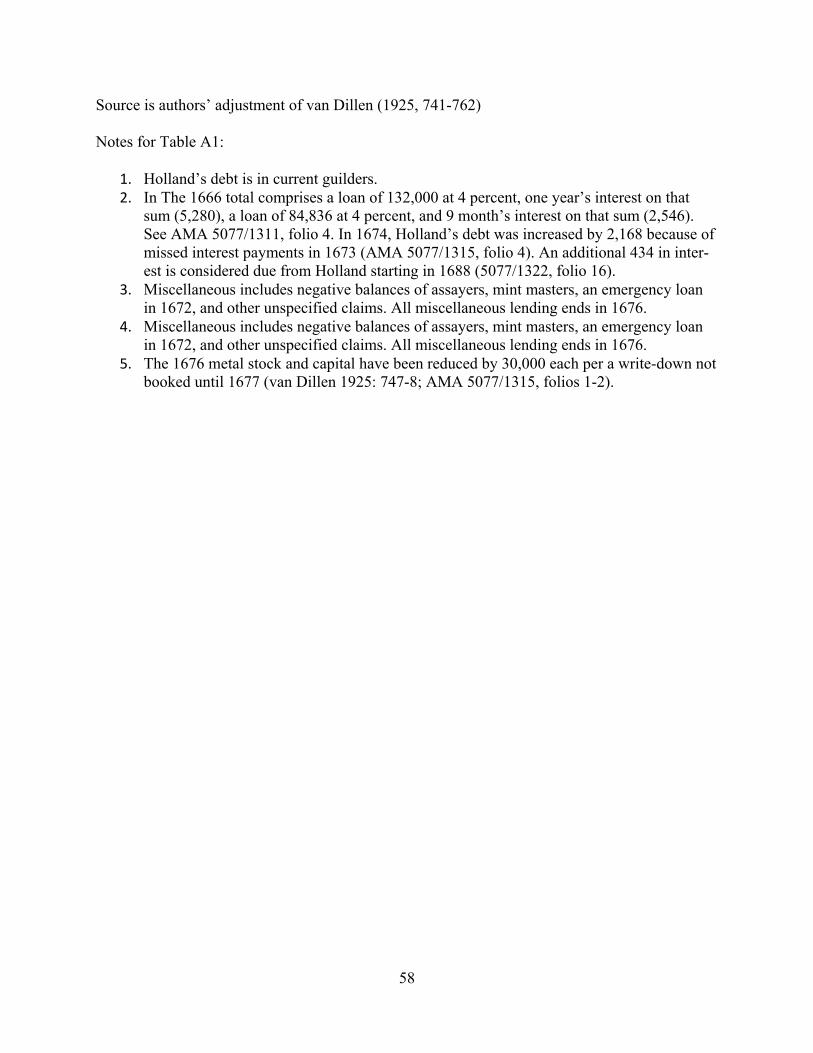
Table A2. Adjusted Capital and Adjusted Loans, Bank Guilders, 1610 to 1795

Jan.

Adjusted Capital

Adjusted Loans

1610 0 0

1611 6,783 0

1612 18,009 71,361

1613 26,276 0

1614 30,277 37,546

1615 30,277 6,000

1616 45,309 98,604

1617 89,912 272,739

1618 118,020 0

1619 138,501 493,198

1620 165,613 239,283

1621 208,390 578,628

1622 252,029 879,476

1623 282,527 1,101,707

1624 146,052 674,635

1625 193,328 1,351,161

1626 140,151 699,041

1627 190,926 1,030,963

1628 233,265 1,266,306

1629 279,496 1,925,131

1630 385,683 1,446,393

1631 447,857 1,255,162

1632 503,164 858,130

1633 542,520 947,854

1634 657,387 1,178,526

1635 748,564 1,192,794

1636 907,639 1,413,671

1637 973,853 1,338,799

1638 1,028,590 1,365,735

1639 1,087,216 1,443,943

1640 1,134,087 1,385,481

1641 1,137,482 837,277

1642 1,139,312 727,691

1643 1,164,660 678,344

1644 1,197,840 590,719

1645 1,154,780 601,739

1646 644,395 466,382

1647 1,006,185 468,281

1648 1,017,687 498,568

1649 1,048,270 668,007

Jan. Adjusted

Capital Adjusted

Loans

1650 780,642 952,332

1651 -171,727 551,353

1652 -287,170 431,214

1653 -426,594 413,160

1654 -408,384 473,593

1655 -371,856 503,510

1656 -335,762 448,308

1657 -324,738 261,122

1658 -320,393 224,661

1659 -308,098 424,941

1660 -393,040 355,994

1661 -370,585 274,661

1662 -368,928 771,411

1663 -489,333 947,770

1664 -461,929 526,712

1665 -430,877 632,448

1666 -426,896 529,586

1667 -402,064 830,612

1668 -359,754 1,142,796

1669 -300,475 1,289,275

1670 -273,412 252,272

1671 -268,021 224,662

1672 -226,844 329,312

1673 -153,983 1,115,601

1674 -221,230 316,949

1675 -208,866 433,882

1676 -145,564 526,831

1677 -134,151 1,042,337

1678 -75,838 1,677,844

1679 -16,226 1,840,163

1680 46,315 1,840,164

1681 94,650 1,235,164

1682 158,217 1,131,831

1683 198,720 899,565

1684 -240,935 632,029

1685 -635,431 226,830

1686 -1,008,520 3,673,747

1687 -706,102 3,897,226

1688 -578,211 2,568,057

1689 -655,984 2,568,056

Jan. Adjusted

Capital Adjusted

Loans

1690 -634,560 2,568,056

1691 -621,847 2,738,978

1692 -621,846 2,738,979

1693 -696,265 2,737,978

1694 -874,938 2,738,978

1695 -981,180 3,138,978

1696 -1,330,917 2,738,978

1697 -925,661 2,738,978

1698 -1,122,803 4,238,978

1699 -2,207,040 3,338,978

1700 -2,192,313 3,238,978

1701 -1,765,126 3,538,978

1702 -1,714,135 4,038,977

1703 -1,645,254 3,438,978

1704 -1,260,493 2,738,978

1705 -1,012,999 3,038,978

1706 -965,929 2,738,978

1707 -928,233 2,938,978

1708 -914,576 2,738,978

1709 -897,183 2,738,977

1710 -873,219 3,638,978

1711 -822,479 4,038,978

1712 -856,337 5,138,978

1713 -754,899 3,438,978

1714 -694,545 3,938,978

1715 -650,803 2,738,979

1716 -598,560 2,738,978

1717 -560,224 2,738,979

1718 -490,558 2,738,978

1719 -434,547 2,738,978

1720 -354,039 2,738,978

1721 -278,386 4,438,978

1722 -114,700 3,538,978

1723 15,259 5,338,978

1724 120,000 6,523,561

1725 149,700 7,723,561

1726 149,202 7,923,560

60

1727 127,595 7,723,561

1728 252,137 7,623,560

1729 357,168 7,723,561

Jan. Adjusted

Capital Adjusted

Loans

1730 75,473 8,323,560

1731 95,267 7,623,560

1732 153,113 6,623,560

1733 115,306 5,523,561

1734 136,117 6,023,560

1735 138,283 5,523,560

1736 48,386 7,423,560

1737 134,486 9,123,560

1738 152,524 9,123,560

1739 181,201 9,623,561

1740 315,011 9,423,560

1741 -335,930 10,923,561

1742 -261,335 11,023,561

1743 -437,044 11,423,560

1744 -226,955 9,323,561

1745 -443,367 8,223,561

1746 -563,412 6,323,560

1747 -886,538 6,823,560

1748 -1,033,812 6,823,560

1749 -1,147,236 5,923,560

1750 -1,247,600 5,523,560

1751 -1,249,450 4,823,560

1752 -1,309,966 4,323,560

1753 -1,107,270 6,973,560

1754 -988,555 8,373,560

1755 -839,638 8,123,561

1756 -676,087 8,023,560

1757 -506,876 8,823,560

1758 -311,706 9,803,560

1759 -115,639 8,603,560

1760 131,221 6,713,560

1761 -18,765 7,023,560

1762 116,261 4,323,560

1763 175,405 4,323,560

1764 119,655 4,323,560

1765 154,629 4,323,560

1766 302,442 4,823,560

1767 401,300 6,423,560

1768 207,653 5,923,561

1769 338,937 5,523,560

1770 447,771 4,323,560

Jan. Adjusted

Capital Adjusted

Loans

1771 -512,590 4,323,561

1772 -463,470 4,323,561

1773 -127,640 4,323,560

1774 -164,582 4,323,560

1775 -253,028 4,323,561

1776 -433,513 4,423,560

1777 -422,304 4,323,560

1778 -365,263 4,323,560

1779 -416,127 5,623,561

1780 -360,838 6,923,560

1781 -460,114 9,123,561

1782 -531,507 10,082,619

1783 -603,214 15,339,227

1784 -618,238 15,586,728

1785 -631,521 16,498,133

1786 -577,466 17,052,037

1787 -2,141,054 15,274,442

1788 -2,115,706 16,639,312

1789 -2,083,569 17,666,574

1790 -2,088,377 16,002,090

1791 -2,065,833 15,256,351

1792 68,696 15,408,846

1793 -27,955 15,426,561

1794 -38,358 15,573,561

1795 -193,672 15,510,418

Source: Authors’ calcula-tion using Van Dillen (1925: 701-807) and AMA 5077/1311 through 1323

61

Table A3. AWB Ledgers and Folios

By Half-Year Periods: a=February to July, b=August to January Date Ledger Folios: Specie Kamer in Bold, Receiver Folios in Regular (kept in sequence by receiver) 1666a 5077/62 147 1174 1391 149 151

1666b 5077/63 1054 1233 1050 1052 1260

1667a 5077/64 982 1149 1249 1387 984 986 988

1667b 5077/65 982 1088 1144 1263 984 986 988

1668a 5077/66 1006 1082 1179 1238 1252 1276 1397 1528 1008 1010

1012

1668b 5077/67 1010 1154 1474 1012 1018 1020

1669a 5077/68 1010 1203 1479 1012 1014 1016

1669b 5077/69 1010 1314 1012 1014 1330 1016 1353

1670a 5077/70 1008 1177 1220 1010 1328 1012 1129 1240 1014 1347

1670b 5077/71 1008 1060 1114 1262 1010 1250 1420 1012 1348 1014 1172 1416 1671a 5077/72 90 1273 1375 1450 1494 1034 1077 1140 1036 1120

1038 1207

1671b 5077/73 1028 1142 1501 1030 1032 1034 1672a 5077/74 990 1415 1433 1439 1449 1455 1461 1465 1478 1488

1496 1501 1076 1078 1080

1672b 5077/75 1044 1047 1046 1220 1048 1050 1673a Missing

1673b 5077/76 1020 1082 1158 1022 1024 1026 1032 1062 258 298

722 1062 1116

1674a 5077/77 878 1209 1303 880 882 884 1674b 5077/78 910 1114 1341 1446 912 914 916

1675a 5077/79 952 1282 1467 954 956 958

1675b 5077/80 974 1217 976 978 980

62

1676a 5077/81 1016 1018 1020 1022 1676b 5077/82 1042 1044 1046 1048

1677a Missing

1677b 5077/83 1044 1494 1046 1048 1050

1678a 5077/84 1078 1452 1080 1082 1084

1678b 5077/85 1058 1060 1062 1064

1679a 5077/86 1021 1022 1023 1024

1679b 5077/87 1008 1332 1421 1009 1010 1011

1680a 5077/88 978 1024 1382 979 980 981

1680b 5077/89 1006 979 980 981

1681a 5077/90 982 979 980 981

1681b 5077/91 982 979 980 981

1682a 5077/92 981 979 1390 980 1396 949

1682b Missing

1683a 5077/94 990 1406 1564 988 1505 989 1052 1296 1351 1514

1683b 5077/96 990 1292 1337 1422 1519 988 994 989 1286 1463

1684a 5077/98 990 1277 1317 1360 1383 1411 1484 1585 988 1518

1567 989 1407 1512 1573 1684b Missing

1685a 5077/101 990 1274 1300 1344 1402 1450 1500 1533 988 1330

1453 989 1334 1427 1484

1685b 5077/103 990 1299 1335 1344 1349 1365 1378 1399 1462 988 1296 1317 1459 1503 1532 989 1300 1321 1411 1470 1508 1531 1686a 5077/105 990 1280 1300 1334 1390 1451 1491 988 1275 1462

1492 989 1313 1408 1471 1494 1686b 5077/107 990 1283 1319 1378 1437 1476 988 1303 1339 1366

1392 989 1284 1310 1335 1358 1369 1402 1470 1492

63

1687a 5077/109 990 1297 1354 1431 1496 988 1291 1322 1353 1376 1413 1465 1491 989 1283 1303 1329 1380 1407 1445 1477 1497

1687b 5077/111 990 1312 1377 1462 1482 1498 1515 1527 988 1290

1315 1347 1383 1412 989 1289 1301 1321 1345 1371 1395 1413

1688a 5077/113 990 1299 1326 1380 1429 1484 1537 988 1378 1450

1511 989 1379 1432 1464 1489 1517 1534 1688b 5077/115 990 1314 1351 1403 1455 1487 1514 1540 988 1354

1393 1420 989 1306 1338 1366 1388 1405 1416 1443 1495

1689a 5077/117 1171 1423 1450 1461 1493 1552 1596 1181 1176 1427

1503 1564 1624 1689b 5077/119 1171 1429 1476 1533 1581 1616 1640 1676 1181 1176

1421 1439 1471 1519 1532 1690a 5077/121 1171 1419 1440 1463 1502 1542 1591 1624 1664 1181

1176 1643 1690b 5077/123 1171 1421 1439 1463 1499 1540 1575 1609 1651 1695

1176 1454 1527 1562 1581 1181 1259 1555 1586 1691a 5077/124 1171 1427 1440 1464 1485 1511 1549 1573 1622 1675

1715 1176 1632 1692 1181 1603 1691b 5077/126 1171 1448 1478 1521 1574 1620 1668 1709 1739 1176

1466 1547 1676 1181 1487 1563 1657 1692a 5077/128 1171 1461 1490 1512 1547 1583 1623 1667 1698 1728

1176 1581 1181 1492 1632 1719 1692b 5077/130 1171 1467 1498 1545 1586 1631 1675 1734 1766 1176

1488 1635 1683 1758 1181 1569 1622 1674 1785 1693a 5077/132 1171 1486 1504 1532 1559 1585 1619 1639 1654 1673

1675 1705 1728 1772 1793 1176 1616 1750 1181 1609 1756

1693b 5077/134 1171 1444 1465 1501 1527 1576 1640 1686 1176 1554

1655 1181 1562 1637 1694a 5077/136 1171 1443 1464 1505 1540 1585 1628 1687 1732 1776

1176 1689 1181 1705 1694b 5077/138 1171 1447 1481 1530 1601 1653 1721 1176 1181 1182

64

1695a 5077/140 1171 1451 1475 1517 1564 1610 1679 1760 1799 1176

1181 1695b 5077/142 1171 1454 1487 1535 1599 1673 1747 1797 1176 1562

1612 1181 1696a 5077/143 1171 1465 1501 1548 1607 1662 1720 1765 1813 1176

1515 1598 1745 1181 1533 1695 1696b 5077/145 1171 1478 1512 1581 1645 1730 1829 1176 1720 1833

1181 1588 1699

1697a 5077/146 1171 1481 1536 1589 1645 1704 1764 1176 1482 1590

1674 1725 1784 1181 1469 1573 1650 1744

1697b Missing 1698a 5077/148 1171 1405 1523 1593 1688 1768 1176 1664 1784 1181

1594 1735

1698b 5077/150 1171 1476 1556 1676 1815 1176 1505 1560 1619 1666 1761 1860 1181 1487 1577 1693 1770 1902

1699a 5077/152 1171 1504 1533 1596 1663 1744 1802 1842 1176 1516 1595 1674 1785 1849 1181 1541 1645 1812

1699b 5077/154 1171 1484 1537 1595 1689 1807 1176 1513 1588 1624 1655 1730 1843 1181 1478 1502 1576 1704 1741 1824

1700a 5077/156 1271 1612 1657 1707 1779 1885 1961 1276 1601 1646

1684 1726 1871 1914 1281 1590 1637 1739 1917 1962

1700b Missing 1701a 5077/158 1271 1659 1734 1829 1939 2002 1276 1597 1700 1743

1799 1895 1967 2020 1281 1607 1622 1643 1665 1719 1810 1872 1946 2003

1701b 5077/160 1271 1629 1670 1737 1805 1878 2011 1276 1601 1609 1624 1712 1801 1932 1281 1639 1733 1859 1960

1702a 5077/162 1271 1627 1691 1779 1848 1935 1276 1647 1704 1825 1928 1281 1630 1685 1765 1847 1983

1702b 5077/164 1371 1732 1785 1866 1934 2003 1376 1916 1381

65

Table A4. Deduced VOC Loans

Loans

Repayments

Date Amount

Date Amount Internal Rate

of Return

7-Jul-71 200,000 → 10-Sep-71 201,446.20 4.06%

17-Jul-71 400,000 → 9-Sep-71 402,410.38 4.07%

24-Jul-71 300,000 → 11-Sep-71 301,643.75 4.08%

4-Aug-71 200,000 → 610576 200,861.50 4.03%

9-Jan-72 100,000

8-Feb-72 100,000 → 9-Mar-72 200,800.00 3.24%

13-Nov-74 100,000 → 4-Dec-74 200,942.45 4.10%

13-Nov-74 300,000 → 2-Apr-75 203,777.70 5.79%1

10-Jan-75 300,000 → 11-Jan-75 300,000.00

9-Jul-75 150,000

13-Aug-75 200,000

28-Aug-75 200,000

7-Sep-75 100,000 → 19-Oct-75 654,710.90 3.97%

18-Sep-75 100,000

3-Oct-75 100,000

4-Oct-75 100,000

9-Oct-75 100,000 → 24-Oct-75 401,022.30 4.06%

31-Jan-83 403,3332 → 4/2/83 101,533.33 4.19%

4/2/83 203,066.65 4.19%

4/2/83 101,533.33 4.19%

4/16/83 200,000 → 11/25/83 204,644.45 3.80%

5/13/83 100,000 → 11/25/83 102,088.80 3.89%

66

6/18/83 100,000 → 11/25/83 101,744.35 3.98%

7/14/83 50,000 → 11/25/83 50,727.73 3.96%

7/20/83 50,000 → 11/25/83 50,677.78 3.87%

8/23/83 50,000 → 11/25/83 50,511.10 3.97%

8/31/83 100,000 → 11/25/83 100,944.48 4.01%

10/26/83 100,000 → 12/3/83 100,400.00 3.84%

11/1/83 100,000

11/9/83 50,000

11/12/83 100,000

11/15/83 100,000 → 12/1/83 350,816.65 3.92%

9/13/83 100,000

10/5/83 100,000

10/12/83 100,000

10/14/83 100,000 → 1/31/843 405,199.00 3.97% Source: Authors’ analysis. Notes

1. De Korte (1984: 66) suggests that the VOC offered 6 percent on anticipations in 1674. 2. Uses the bank’s record of debt due at the start of fiscal year 1683. 3. Used the bank’s record of debt due at the end of fiscal year 1684.

67

Table A5. Municipal Capital Extractions and Injections

Municipal Capital Extractions

Date Type Bank Guilders Current Guilder Agio Used 5/30/82 Account 20,000.00 20,850.00 4 1/4

14-Jan-83 Metal 249,400.50 260,000.00 4 1/4 10-Feb-83 Metal 143,885.00 150,000.00 4 1/41 26-Jan-84 Metal 50,000.00 52,125.00 4 1/41 1-Mar-84 Metal 50,000.00 52,062.50 4 1/81 2-May-84 Metal 96,154.00 100,000.00 41 26-Oct-84 Metal 150,000.00 156,187.50 4 1/81 11-Jan-85 Metal 143,885.00 150,000.00 4 1/41 14-Feb-85 Metal 120,863.30 126,000.00 4 1/4 13-Jul-85 Metal 47,961.65 50,000.00 4 1/4 28-Jul-85 Metal 47,961.65 50,000.00 4 1/4

28-Aug-85 Metal 95,923.30 100,000.00 4 1/4 15-Nov-85 Metal 47,961.65 50,000.00 4 1/4

7-Dec-85 Metal 59,632.60 62,167.00 4 1/4 19-Feb-87 Metal 57,142.85 60,000.00 5 7-Apr-88 Metal 95,238.10 100,000.00 5

23-Jan-93 Metal 95,238.10 100,000.00 5 4-Jun-93 Metal 142,500.00 150,000.00 5 5/192

30-Oct-93 Metal 59,047.60 62,000.00 5 25-Feb-94 Metal 48,976.00 51,458.00 5 20-Jul-94 Metal 95,238.00 100,000.00 5

17-Feb-95 Metal 95,238.00 100,000.00 5 8-Nov-95 Metal 95,238.00 100,000.00 5 11-Jan-96 Metal 190,476.00 200,000.00 5

18-Dec-97 Account 100,000.00 14-Jan-98 Account 100,000.00 28-Oct-98 Account 100,000.00 6-Nov-98 Account 200,000.00 8-Dec-98 Account 200,000.00

25-Nov-98 Account 300,000.00 23-Dec-98 Account 300,000.00 3-Mar-99 Account 100,000.00

18-Mar-99 Account 100,000.00 18-Mar-02 Metal 95,522.40 100,000.00 4 11/16

68

Table A5 Continued Municipal Capital Injections

Date Type Bank Guilder Current Guilder Agio 12-Jun-86 Metal 191,847.00 200,000.00 4 1/4 19-Jul-86 Metal 95,923.00 100,000.00 4 1/4

23-Mar-87 Metal 57,142.85 60,000.00 5 26-Aug-87 Metal 28,571.45 30,000.00 5

4-Sep-87 Metal 28,571.45 30,000.00 5 18-Apr-96 Metal 190,476.00 200,000.00 5

1-Sep-96 Metal 190,476.00 200,000.00 5 28-Mar-99 Account 200,000.00 6-Mar-99 Metal 100,000.00 105,000.00 5 8-Apr-00 Account 400,000.00

Sources: AMA 5077/1311 through 1323. Notes:

1. Imputed from bank guilders (5077/1321 f 7) and current guilders (5077/1322 loose insert). 2. Coins removed in sacks worth 600 current booked at 570 bank: likely dreiguilders

69

Table A6. Large Value and Odd Value Deposits 1666 to 1703

Specie Kamer Receiver Direct Debits1 Debits

Total Deposit Transactions 3,686 17,771 Share of Deposits with guilder values that are

Large Values: Round 100's 6.1% 48.5%

Share of Deposits with guilder values that are Odd Values:

With a Partial Guilder 81.6% 7.4%

With Partial Stuiver (1/20th of a guilder) 10.3% 0.5%

Source: Authors’ calculation. Notes

1. Excludes loan transactions, receiver transfers, and expenditures.

Table A7. AWB Mint Operations, April and May 1668

Guilder Value of Silver Bullion Sent to Various Mint

Mint 27-Apr 1-May 8-May 14-May 30-May Gelderland 22,471.70 28,986.25 27,030.40

Holland 30,284.85 30,105.00 27,837.75 West-Friesland 23,091.80 29,123.60

Utrecht 25,394.55 27,890.45 26,278.85 Friesland 27,419.17

Overijssel 23,877.80 Deventer 26,306.85 Kampen 24,396.55

Zwolle City 24,116.85 27,586.30 27,804.95

Total 99,965.20 99,975.75 115,801.15 27,890.45 136,371.12

Grand Total 480,003.67 Source: AMA 5077/1313

70

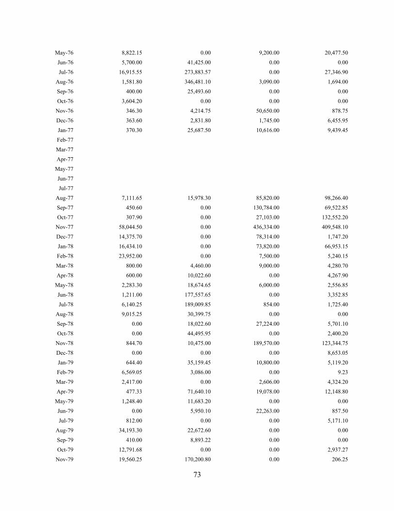
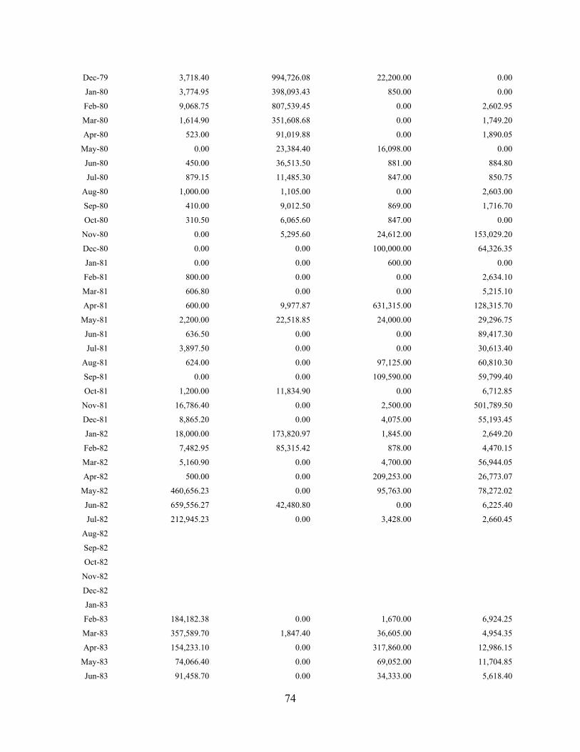
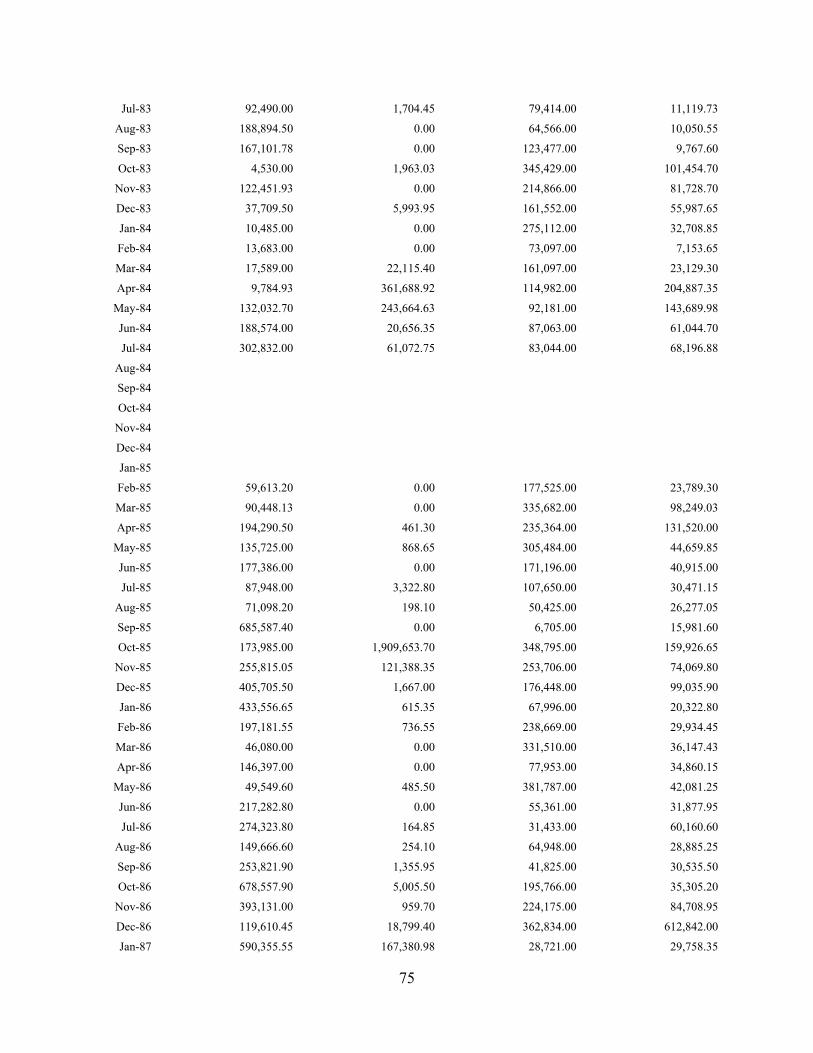
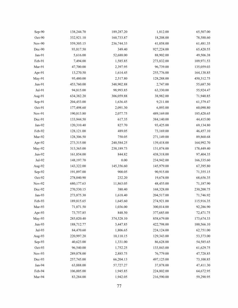
Table A8. Monthly Flows: 1666 to 1703 in Bank Guilders

Guilder Creation by Metal Inflows Guilder Destruction by Metal Outflows

“Coin Deposits”

Receivers “Bullion Purchases”

Specie Camer “Coin Withdrawals”

Round Values “Bullion Sales”

Odd Values

Feb-66 42,281.95 0.00 12,060.00 17,726.88

Mar-66 17,631.75 0.00 421,942.00 15,030.28

Apr-66 55,413.20 346,000.00 227,226.00 105,405.70

May-66 92,164.03 127,501.60 49,448.00 125,898.75

Jun-66 66,628.95 30,000.00 833.00 7,413.03

Jul-66 134,581.98 100,000.00 199,040.00 66,083.47

Aug-66 269,442.73 1,223.75 45,690.00 19,349.83

Sep-66 181,391.53 0.00 85,368.00 15,278.05

Oct-66 6,063.40 0.00 93,501.00 13,460.00

Nov-66 11,344.80 0.00 19,497.00 12,904.00

Dec-66 1,723.10 0.00 97,174.00 105,545.35

Jan-67 0.00 0.00 84,506.00 209,289.35

Feb-67 5,666.95 12,000.00 2,516.00 31,667.90

Mar-67 3,911.75 19,223.10 21,928.00 119,202.98

Apr-67 43,451.53 9,863.75 108,923.00 156,628.80

May-67 20,656.10 17,898.10 146,668.00 57,984.18

Jun-67 9,303.00 13,238.55 22,705.00 44,185.53

Jul-67 9,870.30 30,300.38 32,217.00 72,909.75

Aug-67 1,000.00 12,000.00 79,980.00 27,386.80

Sep-67 12,679.50 42,073.90 189,302.00 107,987.45

Oct-67 2,060.50 0.00 275,652.00 74,613.98

Nov-67 14,537.35 12,000.00 183,364.00 340,681.90

Dec-67 1,074.50 12,000.00 366,740.00 13,159.95

Jan-68 5,775.70 0.00 47,486.00 36,121.00

Feb-68 35,867.35 0.00 188,989.00 76,232.75

Mar-68 8,260.00 6,000.00 303,322.00 77,171.25

Apr-68 10,744.00 330,701.80 299,259.00 139,993.30

May-68 7,128.40 1,437,506.25 300,638.00 147,324.68

Jun-68 5,548.90 82,176.18 68,993.00 90,181.73

Jul-68 19,091.50 61,236.20 93,215.00 99,446.75

Aug-68 23,396.00 34,166.17 22,006.00 30,366.63

Sep-68 12,941.50 5,810.63 13,241.00 38,153.17

Oct-68 7,259.80 44,632.75 56,306.00 45,533.77

Nov-68 13,627.60 44,419.25 183,430.00 31,601.70

Dec-68 14,407.15 0.00 52,315.00 12,496.25

Jan-69 11,376.50 2,391.80 42,000.00 18,943.45

Feb-69 39,286.20 0.00 2,030.00 14,882.90

71

Mar-69 28,162.10 6,000.00 3,772.00 19,579.40

Apr-69 5,600.00 6,000.00 17,290.00 76,818.15

May-69 14,670.00 18,000.00 8,829.00 23,639.25

Jun-69 305.50 20,610.70 14,123.00 8,238.33

Jul-69 39,348.20 15,564.70 27,376.00 21,568.05

Aug-69 67,135.30 18,000.00 5,887.00 9,013.05

Sep-69 53,504.00 73,726.60 5,889.00 7,547.40

Oct-69 36,889.35 0.00 65,291.00 15,060.60

Nov-69 100,741.45 2,387.50 27,079.00 137,058.65

Dec-69 294,380.30 3,888.15 50,335.00 23,614.15

Jan-70 17,923.85 76,000.00 24,009.00 1,659.00

Feb-70 108,314.75 25,748.05 840.00 5,013.75

Mar-70 79,802.30 45,520.48 5,179.00 12,531.00

Apr-70 279,390.38 101,164.38 40,689.00 17,844.63

May-70 200,993.00 483,741.45 125,735.00 10,910.50

Jun-70 125,639.55 148,622.20 11,004.00 16,772.88

Jul-70 121,593.10 0.00 4,432.00 7,919.05

Aug-70 139,628.25 815,231.20 8,283.00 3,355.50

Sep-70 137,260.03 1,415,986.48 257,001.00 573,082.22

Oct-70 91,050.75 229,519.45 75,786.00 26,545.10

Nov-70 74,448.15 131,008.00 91,176.00 21,786.48

Dec-70 121,171.35 139,721.88 148,987.00 30,581.00

Jan-71 243,924.75 128,101.30 52,038.00 7,705.35

Feb-71 277,492.55 59,626.55 2,505.00 7,560.00

Mar-71 293,073.40 2,981.40 18,665.00 844.50

Apr-71 114,742.98 0.00 129,335.00 62,673.20

May-71 274.00 842.70 90,409.00 70,272.75

Jun-71 28,717.65 5,000.00 428,959.00 183,927.55

Jul-71 0.00 0.00 644,761.00 54,174.80

Aug-71 6,006.30 751.25 301,470.00 9,447.50

Sep-71 32,144.80 1,194.25 436,628.00 211,452.98

Oct-71 0.00 0.00 521,353.00 8,430.00

Nov-71 2,100.00 11,378.60 165,363.00 52,643.20

Dec-71 3,005.00 31,694.72 22,267.00 10,776.00

Jan-72 6,608.35 94,975.90 7,526.00 3,357.75

Feb-72 28,985.90 0.00 31,200.00 7,587.00

Mar-72 8,840.00 362.40 2,752.00 43,275.45

Apr-72 17,807.80 1,977.42 4,243.00 7,554.00

May-72 61,561.40 492,991.48 840.00 16,087.50

Jun-72 88,319.22 2,205.00 2,478,372.00 291,351.73

Jul-72 184,624.65 124,543.08 497,630.00 28,198.90

Aug-72 36,767.85 900.00 44,475.00 1,160.65

Sep-72 60,398.10 32,908.30 68,234.00 20,114.50

72

Oct-72 15,109.70 141,521.70 3,807.00 10,978.90

Nov-72 33,357.90 0.00 17,870.00 6,684.00

Dec-72 19,019.50 2,422.05 3,844.00 5,995.50

Jan-73 931.40 81,112.15 13,683.00 11,762.25

Feb-73

Mar-73

Apr-73

May-73

Jun-73

Jul-73

Aug-73 19,496.50 46,196.25 0.00 7,985.15

Sep-73 161,096.95 222,601.32 1,695.00 0.00

Oct-73 198,788.75 272,967.28 0.00 0.00

Nov-73 95,726.95 129,162.38 0.00 0.00

Dec-73 17,608.30 132,844.53 2,460.00 6,897.50

Jan-74 3,007.00 148,456.25 6,771.00 16,868.25

Feb-74 37,689.65 6,380.60 2,231.00 5,937.00

Mar-74 825.30 33,477.60 3,432.00 5,955.00

Apr-74 3,468.70 10,773.95 29,706.00 7,582.38

May-74 1,747.30 31,773.50 175,013.00 31,501.25

Jun-74 1,887.90 84,048.65 138,407.00 25,434.00

Jul-74 0.00 207,612.90 172,931.00 41,257.75

Aug-74 317.30 129,572.48 145,276.00 16,933.65

Sep-74 771.00 31,718.85 15,516.00 34,929.90

Oct-74 10,405.40 18,945.45 61,159.00 42,939.90

Nov-74 1,679.10 69,453.35 76,100.00 9,014.25

Dec-74 6,074.00 17,025.95 110,571.00 10,293.02

Jan-75 0.00 362,830.25 1,698.00 25,602.00

Feb-75 4,338.97 118,484.35 33,487.00 1,707.00

Mar-75 3,019.90 0.00 31,296.00 5,150.68

Apr-75 6,141.00 0.00 75,102.00 170,103.80

May-75 2,495.80 0.00 113,865.00 50,837.07

Jun-75 6,560.60 2,562.50 138,637.00 15,207.50

Jul-75 11,515.90 0.00 161,774.00 0.00

Aug-75 21,882.47 843.75 105,108.00 17,551.13

Sep-75 916.65 0.00 9,366.00 40,367.90

Oct-75 1,250.65 0.00 13,450.00 12,515.82

Nov-75 0.00 0.00 177,964.00 308,633.05

Dec-75 0.00 0.00 15,948.00 132,890.10

Jan-76 8,709.50 24,333.00 25,803.00 39,794.70

Feb-76 13,307.90 0.00 8,319.00 13,891.25

Mar-76 8,828.30 0.00 22,619.00 54,737.50

Apr-76 500.00 0.00 0.00 241,665.50

73

May-76 8,822.15 0.00 9,200.00 20,477.50

Jun-76 5,700.00 41,425.00 0.00 0.00

Jul-76 16,915.55 273,883.57 0.00 27,346.90

Aug-76 1,581.80 346,481.10 3,090.00 1,694.00

Sep-76 400.00 25,493.60 0.00 0.00

Oct-76 3,604.20 0.00 0.00 0.00

Nov-76 346.30 4,214.75 50,650.00 878.75

Dec-76 363.60 2,831.80 1,745.00 6,455.95

Jan-77 370.30 25,687.50 10,616.00 9,439.45

Feb-77

Mar-77

Apr-77

May-77

Jun-77

Jul-77

Aug-77 7,111.65 15,978.30 85,820.00 98,266.40

Sep-77 450.60 0.00 130,784.00 69,522.85

Oct-77 307.90 0.00 27,103.00 132,552.20

Nov-77 58,044.50 0.00 436,334.00 409,548.10

Dec-77 14,375.70 0.00 78,314.00 1,747.20

Jan-78 16,434.10 0.00 73,820.00 66,953.15

Feb-78 23,952.00 0.00 7,500.00 5,240.15

Mar-78 800.00 4,460.00 9,000.00 4,280.70

Apr-78 600.00 10,022.60 0.00 4,267.90

May-78 2,283.30 18,674.65 6,000.00 2,556.85

Jun-78 1,211.00 177,557.65 0.00 3,352.85

Jul-78 6,140.25 189,009.85 854.00 1,725.40

Aug-78 9,015.25 30,399.75 0.00 0.00

Sep-78 0.00 18,022.60 27,224.00 5,701.10

Oct-78 0.00 44,495.95 0.00 2,400.20

Nov-78 844.70 10,475.00 189,570.00 123,344.75

Dec-78 0.00 0.00 0.00 8,653.05

Jan-79 644.40 35,159.45 10,800.00 5,119.20

Feb-79 6,569.05 3,086.00 0.00 9.23

Mar-79 2,417.00 0.00 2,606.00 4,324.20

Apr-79 477.33 71,640.10 19,078.00 12,148.80

May-79 1,248.40 11,683.20 0.00 0.00

Jun-79 0.00 5,950.10 22,263.00 857.50

Jul-79 812.00 0.00 0.00 5,171.10

Aug-79 34,193.30 22,672.60 0.00 0.00

Sep-79 410.00 8,893.22 0.00 0.00

Oct-79 12,791.68 0.00 0.00 2,937.27

Nov-79 19,560.25 170,200.80 0.00 206.25

74

Dec-79 3,718.40 994,726.08 22,200.00 0.00

Jan-80 3,774.95 398,093.43 850.00 0.00

Feb-80 9,068.75 807,539.45 0.00 2,602.95

Mar-80 1,614.90 351,608.68 0.00 1,749.20

Apr-80 523.00 91,019.88 0.00 1,890.05

May-80 0.00 23,384.40 16,098.00 0.00

Jun-80 450.00 36,513.50 881.00 884.80

Jul-80 879.15 11,485.30 847.00 850.75

Aug-80 1,000.00 1,105.00 0.00 2,603.00

Sep-80 410.00 9,012.50 869.00 1,716.70

Oct-80 310.50 6,065.60 847.00 0.00

Nov-80 0.00 5,295.60 24,612.00 153,029.20

Dec-80 0.00 0.00 100,000.00 64,326.35

Jan-81 0.00 0.00 600.00 0.00

Feb-81 800.00 0.00 0.00 2,634.10

Mar-81 606.80 0.00 0.00 5,215.10

Apr-81 600.00 9,977.87 631,315.00 128,315.70

May-81 2,200.00 22,518.85 24,000.00 29,296.75

Jun-81 636.50 0.00 0.00 89,417.30

Jul-81 3,897.50 0.00 0.00 30,613.40

Aug-81 624.00 0.00 97,125.00 60,810.30

Sep-81 0.00 0.00 109,590.00 59,799.40

Oct-81 1,200.00 11,834.90 0.00 6,712.85

Nov-81 16,786.40 0.00 2,500.00 501,789.50

Dec-81 8,865.20 0.00 4,075.00 55,193.45

Jan-82 18,000.00 173,820.97 1,845.00 2,649.20

Feb-82 7,482.95 85,315.42 878.00 4,470.15

Mar-82 5,160.90 0.00 4,700.00 56,944.05

Apr-82 500.00 0.00 209,253.00 26,773.07

May-82 460,656.23 0.00 95,763.00 78,272.02

Jun-82 659,556.27 42,480.80 0.00 6,225.40

Jul-82 212,945.23 0.00 3,428.00 2,660.45

Aug-82

Sep-82

Oct-82

Nov-82

Dec-82

Jan-83

Feb-83 184,182.38 0.00 1,670.00 6,924.25

Mar-83 357,589.70 1,847.40 36,605.00 4,954.35

Apr-83 154,233.10 0.00 317,860.00 12,986.15

May-83 74,066.40 0.00 69,052.00 11,704.85

Jun-83 91,458.70 0.00 34,333.00 5,618.40

75

Jul-83 92,490.00 1,704.45 79,414.00 11,119.73

Aug-83 188,894.50 0.00 64,566.00 10,050.55

Sep-83 167,101.78 0.00 123,477.00 9,767.60

Oct-83 4,530.00 1,963.03 345,429.00 101,454.70

Nov-83 122,451.93 0.00 214,866.00 81,728.70

Dec-83 37,709.50 5,993.95 161,552.00 55,987.65

Jan-84 10,485.00 0.00 275,112.00 32,708.85

Feb-84 13,683.00 0.00 73,097.00 7,153.65

Mar-84 17,589.00 22,115.40 161,097.00 23,129.30

Apr-84 9,784.93 361,688.92 114,982.00 204,887.35

May-84 132,032.70 243,664.63 92,181.00 143,689.98

Jun-84 188,574.00 20,656.35 87,063.00 61,044.70

Jul-84 302,832.00 61,072.75 83,044.00 68,196.88

Aug-84

Sep-84

Oct-84

Nov-84

Dec-84

Jan-85

Feb-85 59,613.20 0.00 177,525.00 23,789.30

Mar-85 90,448.13 0.00 335,682.00 98,249.03

Apr-85 194,290.50 461.30 235,364.00 131,520.00

May-85 135,725.00 868.65 305,484.00 44,659.85

Jun-85 177,386.00 0.00 171,196.00 40,915.00

Jul-85 87,948.00 3,322.80 107,650.00 30,471.15

Aug-85 71,098.20 198.10 50,425.00 26,277.05

Sep-85 685,587.40 0.00 6,705.00 15,981.60

Oct-85 173,985.00 1,909,653.70 348,795.00 159,926.65

Nov-85 255,815.05 121,388.35 253,706.00 74,069.80

Dec-85 405,705.50 1,667.00 176,448.00 99,035.90

Jan-86 433,556.65 615.35 67,996.00 20,322.80

Feb-86 197,181.55 736.55 238,669.00 29,934.45

Mar-86 46,080.00 0.00 331,510.00 36,147.43

Apr-86 146,397.00 0.00 77,953.00 34,860.15

May-86 49,549.60 485.50 381,787.00 42,081.25

Jun-86 217,282.80 0.00 55,361.00 31,877.95

Jul-86 274,323.80 164.85 31,433.00 60,160.60

Aug-86 149,666.60 254.10 64,948.00 28,885.25

Sep-86 253,821.90 1,355.95 41,825.00 30,535.50

Oct-86 678,557.90 5,005.50 195,766.00 35,305.20

Nov-86 393,131.00 959.70 224,175.00 84,708.95

Dec-86 119,610.45 18,799.40 362,834.00 612,842.00

Jan-87 590,355.55 167,380.98 28,721.00 29,758.35

76

Feb-87 342,139.00 3,699.00 33,650.00 33,103.50

Mar-87 421,221.85 5,469.10 1,750.00 38,143.80

Apr-87 464,544.20 21,793.10 3,627.00 42,363.20

May-87 326,724.00 3,694.90 26,803.00 34,675.40

Jun-87 375,232.50 45,386.58 11,283.00 32,011.98

Jul-87 248,930.35 871.20 7,872.00 30,469.48

Aug-87 315,502.50 104,129.25 9,762.00 32,765.25

Sep-87 513,033.00 196,871.55 17,805.00 27,504.10

Oct-87 888,687.70 51,826.15 247,620.00 75,146.45

Nov-87 194,124.60 2,338.00 556,685.00 36,169.25

Dec-87 15,783.00 114,714.03 959,013.00 57,639.93

Jan-88 1,125.00 23,868.02 345,366.00 58,116.10

Feb-88 4,950.00 84,316.90 58,608.00 39,685.00

Mar-88 51,508.50 54,698.22 34,030.00 59,278.55

Apr-88 214,215.10 164,898.08 3,614.00 47,514.00

May-88 251,861.50 41,396.27 125,116.00 51,934.75

Jun-88 444,427.85 109,463.20 3,630.00 42,275.55

Jul-88 478,896.20 100,710.63 30,030.00 37,151.75

Aug-88 285,388.65 3,419.95 48,291.00 51,037.20

Sep-88 289,154.50 114,435.07 78,015.00 32,292.85

Oct-88 846,116.55 35,591.55 36,362.00 38,199.15

Nov-88 487,246.80 143,593.58 539,663.00 38,718.90

Dec-88 133,548.00 264,442.55 740,048.00 33,777.02

Jan-89 13,173.00 42,915.50 485,865.00 29,264.40

Feb-89 122,770.50 49,079.23 39,593.00 36,919.00

Mar-89 169,889.40 49,327.67 143,946.00 56,456.40

Apr-89 16,086.00 24,812.35 598,185.00 135,268.12

May-89 75,954.00 119,297.22 14,085.00 34,649.35

Jun-89 147,739.20 108,929.80 81,399.00 61,867.97

Jul-89 190,473.50 22,660.05 4,486.00 64,139.25

Aug-89 297,603.60 63,848.57 10,608.00 47,095.10

Sep-89 221,104.50 81,086.97 1,206.00 34,513.60

Oct-89 180,741.30 105,669.60 2,650.00 39,152.00

Nov-89 187,760.60 166,762.30 371,373.00 207,432.35

Dec-89 20,400.00 95,522.40 398,868.00 39,476.30

Jan-90 0.00 19,615.45 160,795.00 50,338.92

Feb-90 0.00 78,751.20 66,809.00 54,667.95

Mar-90 0.00 25,945.40 1,650.00 72,894.15

Apr-90 4,740.00 97,700.15 8,495.00 64,903.55

May-90 43,716.00 247,207.68 3,563.00 77,838.10

Jun-90 261,723.00 3,311.60 9,319.00 76,428.95

Jul-90 116,354.30 637.88 890.00 44,439.20

Aug-90 267,780.00 25,868.25 6,299.00 89,145.30

77

Sep-90 138,244.70 189,287.20 1,812.00 65,507.00

Oct-90 332,921.10 160,733.87 18,208.00 78,588.60

Nov-90 559,305.15 236,744.33 41,058.00 61,481.35

Dec-90 93,817.50 349.40 927,224.00 65,420.55

Jan-91 5,616.00 52,688.00 88,902.00 49,506.38

Feb-91 7,494.00 1,585.85 273,832.00 109,971.53

Mar-91 47,700.00 2,397.95 96,739.00 135,059.03

Apr-91 13,270.50 1,614.45 255,776.00 164,138.85

May-91 95,480.00 2,517.80 128,288.00 450,312.75

Jun-91 453,760.00 348,902.88 2,747.00 55,687.50

Jul-91 94,815.00 98,993.85 63,330.00 55,924.47

Aug-91 634,382.20 306,059.88 38,982.00 71,940.85

Sep-91 204,453.00 1,636.45 9,211.00 61,379.47

Oct-91 177,498.60 2,091.30 6,893.00 60,090.80

Nov-91 190,813.80 2,077.75 489,169.00 185,428.65

Dec-91 133,944.50 617.35 384,140.00 44,415.00

Jan-92 120,310.40 827.70 93,425.00 69,134.80

Feb-92 128,121.00 489.05 73,169.00 46,457.10

Mar-92 128,306.50 750.05 271,149.00 89,860.68

Apr-92 273,315.00 240,584.25 139,418.00 164,992.70

May-92 313,365.00 238,189.73 131,074.00 178,449.40

Jun-92 161,854.00 844.82 438,318.00 97,404.35

Jul-92 148,197.70 0.00 234,942.00 166,335.60

Aug-92 143,322.00 145,356.60 145,979.00 67,395.80

Sep-92 191,897.00 900.05 90,915.00 71,355.15

Oct-92 278,040.90 232.20 19,674.00 68,656.35

Nov-92 680,177.63 11,863.05 48,455.00 71,187.90

Dec-92 270,530.15 380.40 168,328.00 230,200.75

Jan-93 273,875.30 1,618.40 204,517.00 71,746.92

Feb-93 189,815.65 1,645.60 274,921.00 115,916.35

Mar-93 71,071.50 1,036.00 300,014.00 92,286.90

Apr-93 73,757.85 848.50 377,685.00 72,471.75

May-93 285,020.40 374,528.10 858,679.00 173,674.33

Jun-93 188,712.77 3,447.85 422,798.00 100,566.10

Jul-93 84,470.60 1,806.65 224,124.00 62,751.00

Aug-93 220,997.20 10,110.15 129,343.00 53,373.00

Sep-93 40,623.00 1,331.00 86,628.00 54,585.65

Oct-93 96,540.00 1,752.25 133,843.00 61,629.75

Nov-93 289,878.00 2,885.75 76,779.00 47,728.85

Dec-93 257,745.00 66,204.13 497,125.00 73,100.85

Jan-94 63,888.00 57,727.27 37,878.00 47,411.30

Feb-94 106,005.00 1,945.85 224,802.00 64,672.95

Mar-94 83,284.00 1,942.05 216,590.00 59,290.95

78

Apr-94 15,747.00 125,121.53 292,345.00 49,925.35

May-94 55,410.00 1,022,275.45 228,580.00 56,609.60

Jun-94 207,507.00 298,151.93 98,022.00 65,563.80

Jul-94 43,857.00 182,252.77 50,948.00 58,163.90

Aug-94 62,349.00 576,368.20 101,476.00 57,266.95

Sep-94 10,125.00 2,813.90 226,467.00 47,678.05

Oct-94 26,592.00 64,115.20 112,239.00 44,143.40

Nov-94 25,737.00 20,463.10 309,909.00 300,312.27

Dec-94 40,506.00 128,805.57 365,157.00 85,704.35

Jan-95 35,118.00 179,740.70 6,621.00 31,202.80

Feb-95 46,684.30 2,856.00 15,919.00 44,765.20

Mar-95 27,636.00 2,108.25 123,943.00 65,230.60

Apr-95 4,986.00 22,366.80 281,830.00 43,157.00

May-95 22,184.30 24,468.50 204,971.00 49,828.00

Jun-95 49,196.50 137,404.30 79,836.00 253,656.63

Jul-95 0.00 2,749.98 84,212.00 291,572.30

Aug-95 3,600.00 3,921.00 53,507.00 44,850.70

Sep-95 59,589.00 11,351.55 61,854.00 36,098.30

Oct-95 205,669.50 5,652.00 13,261.00 244,618.50

Nov-95 130,863.80 28,858.40 224,037.00 46,820.13

Dec-95 55,140.00 85,730.80 58,571.00 42,127.75

Jan-96 88,128.20 32,675.23 19,889.00 58,477.55

Feb-96 179,979.10 6,673.15 115,244.00 76,721.75

Mar-96 149,403.00 8,008.20 17,372.00 57,250.90

Apr-96 137,732.30 36,303.23 70,171.00 56,238.75

May-96 138,771.00 304,043.18 123,066.00 66,894.90

Jun-96 133,998.00 96,978.43 181,541.00 62,116.70

Jul-96 34,402.00 72,280.38 22,573.00 56,540.10

Aug-96 100,982.00 101,314.52 15,132.00 57,564.85

Sep-96 25,954.50 34,728.65 248,374.00 38,865.85

Oct-96 80,223.60 38,853.70 47,562.00 235,678.85

Nov-96 97,574.70 10,353.35 99,833.00 86,673.35

Dec-96 155,232.55 45,018.80 290,850.00 30,647.15

Jan-97 123,383.20 161,004.30 7,788.00 69,762.35

Feb-97 199,219.70 90,696.00 7,148.00 41,515.45

Mar-97 216,923.00 46,972.95 63,253.00 49,048.90

Apr-97 251,432.00 44,003.20 697,509.00 47,140.00

May-97 502,977.85 30,159.32 155,454.00 93,267.90

Jun-97 547,987.40 30,686.30 13,417.00 57,735.30

Jul-97 452,420.00 21,096.45 3,751.00 38,411.25

Aug-97

Sep-97

Oct-97

79

Nov-97

Dec-97

Jan-98

Feb-98 51,042.00 1,835.25 12,892.00 23,016.12

Mar-98 216,798.00 15,189.48 142,377.00 29,509.90

Apr-98 6,888.00 33,180.12 233,110.00 237,245.33

May-98 402,185.30 42,003.20 207,678.00 37,903.92

Jun-98 179,351.90 8,420.30 13,471.00 57,640.02

Jul-98 154,964.40 3,751.15 22,442.00 67,041.35

Aug-98 255,661.00 78,688.35 373,486.00 47,891.60

Sep-98 329,362.90 528.45 365,242.00 49,625.30

Oct-98 409,924.90 706,765.30 3,220.00 40,335.27

Nov-98 300,261.20 899,359.70 780,586.00 25,894.67

Dec-98 199,486.90 71,153.55 426,599.00 34,842.73

Jan-99 239,540.70 5,278.60 4,849.00 34,341.58

Feb-99 202,214.50 0.00 226,775.00 50,755.60

Mar-99 244,456.00 300,000.00 516,603.00 162,951.07

Apr-99 135,708.00 1,049.40 38,544.00 126,532.97

May-99 116,241.00 836.65 143,258.00 85,931.45

Jun-99 305,985.40 0.00 258,471.00 114,059.22

Jul-99 193,570.50 541.75 131,634.00 209,086.80

Aug-99 281,760.00 0.00 12,393.00 95,752.83

Sep-99 230,132.50 15,454.98 20,595.00 57,793.25

Oct-99 202,075.00 669.20 87,109.00 117,560.53

Nov-99 343,926.55 0.00 250,785.00 49,087.97

Dec-99 338,751.00 0.00 473,692.00 38,129.68

Jan-00 295,651.00 887.00 162,391.00 49,528.42

Feb-00 414,494.00 0.00 92,656.00 49,365.63

Mar-00 294,717.00 0.00 287,522.00 101,260.07

Apr-00 202,891.60 1,418.90 888,665.00 46,190.45

May-00 113,160.00 35,782.25 1,904.00 57,833.35

Jun-00 158,005.00 78,574.32 13,019.00 51,952.15

Jul-00 217,719.70 42,656.53 14,613.00 75,711.50

Aug-00

Sep-00

Oct-00

Nov-00

Dec-00

Jan-01

Feb-01 1,000,918.00 76,062.00 10,842.00 15,740.85

Mar-01 295,339.00 15,252.60 78,514.00 101,112.77

Apr-01 438,613.65 33,020.80 898,806.00 79,438.60

May-01 476,311.20 12,616.00 31,606.00 55,779.05

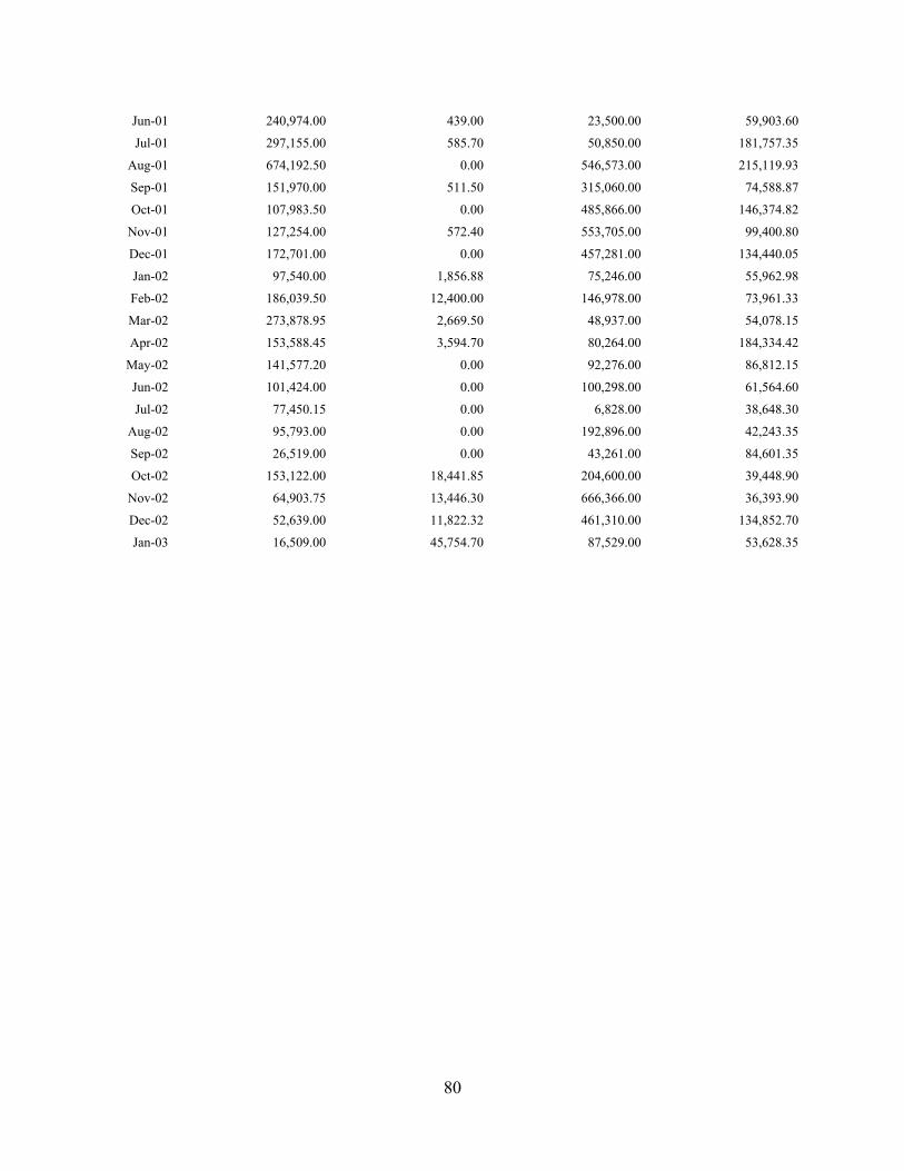
80

Jun-01 240,974.00 439.00 23,500.00 59,903.60

Jul-01 297,155.00 585.70 50,850.00 181,757.35

Aug-01 674,192.50 0.00 546,573.00 215,119.93

Sep-01 151,970.00 511.50 315,060.00 74,588.87

Oct-01 107,983.50 0.00 485,866.00 146,374.82

Nov-01 127,254.00 572.40 553,705.00 99,400.80

Dec-01 172,701.00 0.00 457,281.00 134,440.05

Jan-02 97,540.00 1,856.88 75,246.00 55,962.98

Feb-02 186,039.50 12,400.00 146,978.00 73,961.33

Mar-02 273,878.95 2,669.50 48,937.00 54,078.15

Apr-02 153,588.45 3,594.70 80,264.00 184,334.42

May-02 141,577.20 0.00 92,276.00 86,812.15

Jun-02 101,424.00 0.00 100,298.00 61,564.60

Jul-02 77,450.15 0.00 6,828.00 38,648.30

Aug-02 95,793.00 0.00 192,896.00 42,243.35

Sep-02 26,519.00 0.00 43,261.00 84,601.35

Oct-02 153,122.00 18,441.85 204,600.00 39,448.90

Nov-02 64,903.75 13,446.30 666,366.00 36,393.90

Dec-02 52,639.00 11,822.32 461,310.00 134,852.70

Jan-03 16,509.00 45,754.70 87,529.00 53,628.35

81

Table A9. Calculation of Withdrawal Revenue

Fiscal Year Revenue

Change in VOC

Interest Due VOC Inter-

est Holland Interest

"Withdrawal" Revenue

Metal Outflow through

Specie Kamer

Ratio

1666 39,934 -4,025 -11,750 -8673 15,487 2,049,670 0.76%

1667 57,861 -2,361 -26,667 -8673 20,141 2,560,011 0.79%

1668 74,949 -10,022 -35,933 -8673 20,340 2,431,159 0.84%

1669 42,313 18,333 -46,283 -8673 5,690 610,589 0.93%

1670 20,861 0 0 -8673 12,189 1,555,197 0.78%

1671 56,491 0 -6,362 -8673 41,633 3,344,676 1.24%

1672 88,594 0 -800 -8673 79,119 3,617,700 2.19%

1673

1674 28,794 0 -942 -8673 19,177 1,189,420 1.61%

1675 49,354 0 -8,489 -8673 32,193 1,696,559 1.90%

1676 57,506 -15,507 -32,678 -8673 647 482,826 0.13%

1677 74,023 -35,506 -5,509 -8673 24,336

1678 74,636 37,680 -99,455 -8673 4,186 417,590 1.00%

1679 78,004 0 -64,000 -8673 5,332 92,651 5.75%

1680 63,534 5,000 -56,111 -8673 3,750 374,407 1.00%

1681 79,889 3,333 -41,789 -8673 32,760 1,842,897 1.78%

1682 56,497 1,667 -31,745 -8260 18,159

1683 42,598 -1,866 -18,689 -8260 13,782 2,068,942 0.67%

1684 64,987 5,199 0 -8260 61,926 Source: van Dillen 1925: 701-807, and authors’ calculation.

82

Table A10. The VOC-AWB Credit Relationship

1 2 3 4 5 6

AWB Loans

VOC External Debt

FY Ending in bank guilders in current guilders

AWB's Share AWB Lending

VOC Expenditures

AWB’s Share

4/30/1667 300,000 12,068,477 3% 300,000 7,767,160 4%

4/30/1668 600,000 14,776,188 4% 800,000 10,358,418 8%

4/30/1669 1,100,000 15,584,693 7% 1,600,000 9,962,440 17%

4/30/1670 100,000 14,205,462 1% 500,000 7,408,009 7%

4/15/1671 0 12,254,925 0% 0 8,042,724 0%

4/15/1672 0 11,779,872 0% 1,300,000 8,440,686 16%

4/15/1673 0 14,456,424 0% 0 5,970,759 0%

4/15/1674 0 13,392,636 0% 0 4,863,855 0%

4/15/1675 0 12,558,813 0% 700,000 8,688,494 8%

4/15/1676 0 13,099,801 0% 1,850,000 8,960,247 22%

4/15/1677 1,200,000 11,513,962 11% 700,000 9,553,385 8%

4/15/1678 800,000 12,289,233 7% 1,600,000 8,277,794 20%

4/15/1679 1,500,000 12,205,185 13% 100,000 5,953,366 2%

5/31/1680 1,600,000 11,175,629 15% 0 8,238,865 0%

5/31/1681 1,300,000 11,050,717 12% 0 8,030,878 0%

5/31/1682 1,000,000 10,397,454 10% 500,000 8,738,099 6%

5/31/1683 600,000 8,254,522 8% 1,500,000 7,711,769 20%

5/31/1684 0 8,509,926 0% 1,200,000 7,902,883 16%

5/31/1685 400,000 9,320,289 4% 1,200,000 9,342,818 13%

5/31/1686 1,200,000 9,379,135 13% 2,600,000 9,213,639 29%

5/31/1687 1,800,000 8,526,588 22% 2,100,000 9,101,201 24%

5/31/1688 2,000,000 7,618,671 27% 1,000,000 9,762,741 11%

5/31/1689 600,000 7,168,758 9% 1,200,000 9,084,777 14%

5/31/1690 700,000 7,502,565 10% 1,000,000 8,679,884 12%

5/31/1691 600,000 6,540,960 10% 200,000 8,737,656 2%

5/31/1692 0 6,930,417 0% 1,400,000 8,056,246 18%

5/31/1693 0 6,566,856 0% 400,000 11,020,009 4%

5/31/1694 0 7,172,006 0% 1,800,000 10,718,641 18%

5/31/1695 200,000 7,134,778 3% 1,950,000 10,275,190 20%

5/31/1696 250,000 6,578,286 4% 1,150,000 11,217,275 11%

5/31/1697 0 7,441,164 0% 1,900,000 11,153,469 18%

5/31/1698 0 8,790,546 0% 3,000,000 8,863,991 35%

5/31/1699 0 7,637,538 0% 1,200,000 15,054,157 8%

5/31/1700 0 7,565,911 0% 1,300,000 11,332,523 12%

5/31/1701 0 8,723,226 0% 3,600,000 13,783,169 27%

5/31/1702 1,000,000 8,730,226 12% 3,300,000 12,399,812 28% Source: VOC data from de Korte (1984: 1A-1C).

83

Appendix B. Theoretical illustrations

This appendix offers a formal examination of the efficiency gains stemming from changes

in the AWB’s credit policies following the 1683 reform. The model environment considered

builds in a natural financial intermediary and payments provider role for the Bank of Amster-

dam, i.e., the bank is endowed with advantages in these capacities. The model then traces

through the consequences of the bank’s transition to a fiat standard.

Time is discrete and infinite in the model environment. Time is indexed by t, and each pe-

riod (which can be thought of as a “year” for convenience) is subdivided into 3 stages {0,1,2},

referred to as winter, spring/summer, and autumn. There are 2 classes of agents, domestic and

foreign. Foreign agents have measure 1 and domestic agents have measure ½.49 Agents are ex

ante identical within a class. Domestic agents coordinate their production and consumption deci-

sions and function as a single agent. In addition to private agents, there is an exchange bank

whose activities are described below. Economic activity takes place in 2 locations, the domestic

economy (“Amsterdam”) and elsewhere (“abroad”).

Synopsis of the model

The model incorporates a stylized cycle of trade. Foreign agents (natural lenders) earn silver

abroad in the winter and bring it to Amsterdam in spring, in search of trading opportunities. Sil-

ver is exchanged with the coalition of domestic agents (a natural borrower) in return for bank

money that can be used to purchase goods in Amsterdam. Domestic agents use the silver they

obtain for consumption abroad, while engaged in productive activities (overseas expeditions) that

do not return goods until the autumn of the same year.

At the beginning of autumn, some foreign agents experience a liquidity (i.e., preference)

shock, meaning they must depart Amsterdam in order to consume. Also in autumn, goods arrive

in Amsterdam from summer productive activities undertaken by domestic agents. Foreign agents

not experiencing a liquidity shock may either purchase these goods with bank money, or may

choose to liquidate their bank balances for silver, which can then be used to purchase consump-

tion goods abroad. Table 1 summarizes the timing of actions in the model.

49 The labels “domestic” and “foreign” are more handy than accurate. “Long-term participants in the Amsterdam markets” and “opportunistic participants” might be more exact.

84

Table 1: Timing of actions in the model

Time of year Foreign agents

(overlapping generations) Domestic agents (infinitely lived)

Winter (stage 0) Young foreign agents trade production goods abroad for silver

Spring (stage 1a) Young arrive in Amsterdam; trade silver for bank money; old (liquidity constrained) trade

money for silver and depart Amsterdam

Trade money for silver in Amsterdam

Summer (stage 1b)

Old, liquidity-constrained agents purchase con-sumption goods abroad

Use silver to purchase consumption abroad;

Begin production Early autumn

(stage 2a) Liquidity shock revealed for young agents Goods arrive in Amster-

dam from summer pro-duction

If liquidity shock If no shock Autumn (stage

2b) No action; wait to

trade money for sil-ver next period

Use money to purchase goods from domestic

agents & consume

Sell goods to domestic agents for money

Commodities and feasible trades

There are 3 commodities: a nondurable general consumption good, a nondurable special con-

sumption good, and a durable good, silver, which is used for only for trade. Silver can be stored

at negligible cost.

All trading outside Amsterdam is of silver for the other goods, and always at the world price

of φ units of silver per good, normalized to 1φ = for both goods. All trading within Amsterdam is

of goods for money (bank balances, described below). For expositional clarity, domestic agents

may not purchase silver by issuing IOUs to foreign agents.50 Likewise, foreign agents may not

directly purchase special goods from domestic agents with silver, but must use money to make

their purchases. Finally, domestic agents must sell their special good production in their “home

market,” Amsterdam.

50 This constraint could be partially relaxed without qualitatively changing the model results. What matters is that foreign agents are less willing to accept domestic agents’ debt than is the bank.

85

Preferences, endowments, and technologies

Each generation of foreign agents lives for 2 years. A generation-t foreign agent is born

abroad in stage 0 of the year t and can produce 0tx units of the general good for sale on the world

market. He (typically) journeys to Amsterdam in stage 1, although the agent always has the op-

tion of remaining abroad and trading exclusively in the world market. At the beginning of stage

2, a foreign agent experiences a shock that determines his preferences for general good versus

special good consumption. The utility of a generation-t foreign agent i is

0 2 1, 1 2 2( ) (1 ) ( )i i i i it t t t t tU x u c u fλ β λ+= − + + − (4)

where β is an annual discount factor, 1, 1i

tc + represents i’s consumption of the general good (which

takes place in the summer of year 1t + ), 2itf represents his consumption of the special good

(which typically takes place in the autumn of year t),51 2itλ is a preference shock, and u is a con-

cave utility function. To allow for analytic results, we take (1 )( ) /(1 )u c c ρ ρ−= − where (0,1)ρ ∈ .

The probability distribution for 2tλ is

2

,1 with probability ½0 with probability ½ .tλ⎧

= ⎨⎩

(5)

An agent who receives a preference shock 2 1tλ = is said to be “liquidity constrained,” in the

sense that the agent only wants to consume the general good, which is only available abroad for

silver. The remaining (called “unconstrained”) foreign agents want to consume the special good,

either abroad or in Amsterdam, depending on market conditions. An agent’s type (constrained or

not) is private information.

Domestic agents are infinitely lived and have objective

( )1 10

tt t

tV d axβ

∞

=

= −∑ (6)

where 1td is the agent’s summer (stage 1) consumption of the general good abroad, 1tx is the

summer production of the special good undertaken by the agent, and (0, )a β∈ . There is no dis-

counting from spring to autumn. Productive effort 1tx yields 2 1t ty x= special goods which are

brought to Amsterdam. Domestic agents cannot earn silver abroad, so silver for their general

51 This is a slight abuse of notation: the special good may also be purchased on the world market and consumed in the spring of the next year, although this does not occur in the equilibria we consider.

86

good consumption must be obtained through trade in Amsterdam with foreign agents. Foreign

agents have an incentive to trade with domestic agents in the Amsterdam market, since domestic

agents can produce the special good at a cost below the world price of one.52

Silver can be held by domestic agents, foreign agents young or old, or the exchange bank

(described below). Let ( )1 1y ot tS S be the per-capita, non-negative amount of silver held by old for-

eign agents at the end of stage 1a money market trading, and let ( )1 2d dt tS S be domestic agents’

stage 1a (stage 2) per-capita silver holdings (again nonnegative). The amount of silver (per do-

mestic resident) held at the exchange bank after stage 1(2) trading is ( )1 2b bt tS S .

Efficient steady-state allocations

As a benchmark, we first consider efficient steady-state allocations. The planner maximizes

the population-weighted discounted utility of all agents, i.e.,

( )0

/ 2 tt

tW V E Uβ

∞

=

= +∑ (7)

over allocations ( )0 1 1 1 2 1 1 1 2 1, , , , , , , , ,y o d d bt t t t t t t t t tx x d c f S S S S S . Feasibility constraints are

0 2, 1 1, 1 1, 1 1, 1, 1 12 2 2d b y y o d bt t t t t t t tx S S S S S S S− − −+ + + ≥ + + + , (8)

1 1ot tS c≥ , (9)

1, 1,dt tS d≥ (10)

1 2t tx f≥ . (11)

Constraint (8) says that the total silver available to the Amsterdam economy in stage 1a consists

of silver imported by young foreigners plus any silver stored by domestic agents, the bank, and

old foreigners. Constraint (9) says that the general good consumption of foreigners is limited by

the amount of silver they have available. A similar constraint (10) applies to consumption by

domestic agents. Constraint (11) is the resource constraint on special good consumption by for-

eigners. The truth-telling condition for the planner’s problem is

2 1, 1( ) ( )t tu f u cβ +≥ , (12)

52 I.e., the law of one price does not hold for special goods. Sufficient frictions operate in the background to allow this situation to persist.

87

i.e., an unconstrained foreign agent must do at least as well by consuming domestically as he

could by reporting himself as a constrained agent, accepting a silver payment, and then using the

silver to purchase the special good abroad the following year. Participation constraints for for-

eign and domestic agents are

, 0EU V ≥ . (13)

The set of planner’s allocations (superscript p) is described as

,1 1 1( ) 1, i.e., 1p p o pu c c S′ = = = (14)

(1/ )2 2 1( ) , i.e.,p pu f a f x a ρ−′ = = = (15)

,1 1 2 1 2 1, , where ( ) ( )p d p p p p pd S af d d u c u f c⎡ ⎤= ∈ = + −⎣ ⎦ (16)

0 1 12 p px c d= + (17)

, , ,2 1 1 0d p b p y pS S S= = = (18)

Conditions (14) and (15) are standard optimality conditions. Note that truth-telling condition (12)

does not bind in the planner’s allocation. Condition (16) says that domestic agents’ consumption

is indeterminate between the bounds imposed by individual rationality for both classes of agents.

Condition (17) says that silver imports by young foreigners must be sufficient to cover general

good consumption by domestic agents and old foreigners. Silver carries an opportunity cost and

has no liquidity value over the winter, so the planner sets inter-period holdings of silver by do-

mestic agents, the bank, and foreigners equal to zero (condition (18)).

The exchange bank

Money takes the form of balances at an exchange bank. Initially we assume the bank does

not engage in lending. More specifically, the exchange bank credits any deposits of silver into

the exchange bank at a fixed number of units of silver θ per florin of bank money, normalized to

1θ = . Withdrawals from the bank occur at a mandated price 1θ < .

In the decentralized economy, money can be traded for silver in stage 1a. The market value

of money in terms of silver is θ units of silver per unit money (“florin”).53 Absence of arbitrage

53 I.e., the price of bank money is proportional to one plus the agio. As explained above, the actual agio expressed the price of bank money relative to current money, whose metallic value could vary over time. While a model of current money valuation could be incorporated in to the model, we abstract from this complication to keep notation manageable.

88

requires that the market price of bank money be in the interval [ ,1]θ . As long as the market price

of money is in this interval, there is (weakly) no incentive for agents to deposit or withdraw sil-

ver from the bank: hence, for steady states (i.e., for constant θ ) we exclude the possibility of

deposits or withdrawals.

However, anyone with funds at the exchange bank has the option of withdrawing funds from

the bank at any time. Suppose that at a given moment the bank has liabilities (accounts) of M

florins per domestic resident and holds bS units of silver (“coins”) in its vault. Strictly speaking,

the depositors’ right of withdrawal means that the exchange bank faces a liquidity constraint on

its metal-to-deposit ratio /bS M 54

/bS M θ≥ . (19)

Taken at face value, this would require that the bank maintain a metal-to-deposit ratio of around

98 percent. As we have seen above, in practice the AWB was generally able operate with a

smaller ratio. Hence (19) is modified to

/bS M δθ≥ , (20)

for some “comfort factor” 1δ < .

The special consumption good is traded in Amsterdam in stage 2 at money price tp . Since

unconstrained foreigners can choose where to consume the special good in stage 2, the silver-

equivalent price of special goods in Amsterdam ( )t t tpσ θ≡ (i.e., the terms of trade for domestic

agents) can be no greater the silver price of goods abroad (one).

Steady-state monetary equilibria

In the decentralized economy, young foreign agents wishing to purchase goods in Amster-

dam must first use their silver earnings to purchase money holdings 1ytM . Foreign agents maxi-

mize the expectation of utility (4) over 0x , 1c , 2f , 1yM , and 1

yS , taking prices as given, subject

to budget constraints

0 1 1y y

t t t tx M Sθ= + (21)

54 Following the Diamond-Dybvig tradition, constraint (19) could be motivated as necessary to prevent sunspot-based runs on the exchange bank. Runs can occur since types are unobservable and unconstrained agents can always obtain the special good abroad.

89

1 1 1 1, 1y y

t t t tM S cθ + ++ ≥ (22)

2y

t t tM p f≥ (23)

Steady-state optimality conditions for foreign agents reduce to

( )2 2(½) ( ) ( )u f u fβσ σ σ′ ′+ = (24)

In addition, it can be shown that a young foreign agent will always liquidate his silver earnings

for money. If he is unconstrained, he will spend this money to purchase the special good; if he is

constrained, he will trade it the following year to obtain silver to purchase the general good.

Condition (24) implicitly defines a function 2( )g fσ = where g can be shown to be strictly

decreasing and strictly convex for coefficient of relative risk aversion (0,1)ρ ∈ . The inverse

demand curve for special goods 2( )fσ is then given by

22

2 2

1, for 1 ,( )

( ), for 1.f

fg f f

σ<⎧

= ⎨ ≥⎩ . (25)

The kink in the inverse demand curve occurs because the domestic silver-equivalent price for the

special good cannot exceed the world price of unity. Domestic agents’ total revenue from special

good sales can then be expressed as

2 2 2( ) ( )TR f f fσ= (26)

which can be shown to be strictly increasing and concave (strictly for 2 1f > ).

A domestic agent in the decentralized economy maximizes his objective (6) subject to stage

1a, stage 1b, and stage 2 budget constraints

2, 1 2, 1 1 1d d d d

t t t t t tS M S Mθ θ− −+ ≥ + (27)

1 1 2d dt t tS d S≥ + (28)

1 1 2d dt t t tM p x M+ ≥ (29)

over 1 1 1 2 1 2, , , , ,d d d dt t t t t td x S S M M where d

itM denotes the agent’s money holdings at the end of stage i

of period t. Production decisions 1tx are made cooperatively, i.e., production is set so as to

maximize monopoly profits. Steady-state first-order conditions for domestic agents reduce to

[ ] ( )11

1, if (1) /

/ , if (1) /

TR ax

TR a TR a

β

β β−

′ <⎧⎪= ⎨′ ′ ≥⎪⎩

(30)

90

where TR′ is the right derivative of TR. That is, the coalition of domestic agents sets marginal

revenue TR′ from its sales of the special good equal to marginal cost (where the latter is adjusted

for the time cost of money), if this cost is sufficiently low. Otherwise, domestic agents produce

just enough of the special good to equate its silver-equivalent price in Amsterdam to the world

price.

A steady-state monetary equilibrium is an allocation, combined with a set of per-capita

money holdings 1yM , 1

dM , 2dM , and prices p and 1 2( )θ θ θ= = , for which (a) first-order condi-

tions (24) and (30) hold, and (b) markets clear. Money market clearing in particular requires

2 1 1d y dM M M= + , (31)

i.e., that sales of money by domestic agents 2 1d dM M− plus sales by old foreigners 1

yM equal

purchases by young foreigners 12 yM . Equilibria are described as

Proposition 1. There is a continuum of steady-state monetary equilibria where

(1) Allocations, the silver-equivalent price of special goods pσ θ= , and the real stock of

bank money are the same in every equilibrium;

(2) The price of money and the money price of special goods are indeterminate in the inter-

vals [ ],1θ θ∈ , ,p σσθ

⎡ ⎤∈ ⎢ ⎥⎣ ⎦

;

(3) The nominal money stock varies with θ the according to

1 /M d θ= (32)

where 1d is the equilibrium consumption of the general good by domestic agents;

(4) Money is held exclusively by foreigners over the summer, and by domestic agents and

old foreigners over the winter

2 1 1; 0 ;d y dM M M M= = = (33)

(5) Neither domestic nor foreign agents store silver over the winter

2 1 1 0 ;d y oS S S= = = (34)

(6) The exchange bank stores sufficient silver to satisfy its liquidity constraint (20)

( )1 2 1/ .b bS S M dδθ δ θ θ= = = (35)

91

Proof (Sketch). There are two cases to consider.

Case 1: (1) /TR a β′ < . In this case the equilibrium allocation can be derived as follows: from

(30), domestic agents produce just enough special goods to satisfy demand at the world silver-

equivalent price of one, so 1σ = . From inverse demand (25) and market clearing, it follows that

1 2 1d f= = . Using budget constraints (21) and (23), it follows that 1 1c = .

The rest of the equilibrium is then constructed as follows. Absence of arbitrage in the money

market requires [ ],1θ θ∈ ; hence if σ is determined it must be the case that ,p σσ

θ⎡ ⎤∈ ⎢ ⎥⎣ ⎦

. For do-

mestic agents, holding silver over the summer is clearly dominated by consumption, hence their

summer money holdings are zero. All winter asset holdings by domestic agents then take the

form of money as in (32), and in equilibrium this must equal money expenditure by the uncon-

strained foreign agents as in (33).

Case 2: (1) /TR a β′ ≥ . In this case, from (30), domestic agents optimally produce

[ ] 12* ( / )x TR a β−′= , hence 2 2 2* *f f x= = from market clearing. Then from inverse demand (25),

2* ( *) 1fσ σ σ= = < ; using budget constraints (21)-(23) and (27)-(29), and market clearing, it

follows that *1 1 1 2 2 2* ( *) ( *)c d d f f TR fσ= = = = . The rest of the equilibrium is constructed as in

the previous case.

Corollary. Any steady-state monetary equilibrium in the decentralized economy is inefficient.

Proof. In case 1, the equilibrium domestic agents’ general good consumption 1d and foreign

agents’ general good consumption 1c is in the set of planner’s allocations described by (14)-(18).

However, monopoly pricing by domestic agents causes the foreign agents’ consumption of the

special good 2f to fall below its efficient value.

In case 2, foreign agents again underconsume the special good relative to the planner’s allo-

cation due to monopoly pricing. Since foreign agents’ general good consumption (=domestic

agents’ consumption = TR) is greater than one in this case, it follows that foreign agents also

overconsume the general good.

92

In both cases, the relative price of the special good is higher than the corresponding shadow

price a in the planner’s allocation. Also, in both cases the bank inefficiently stores silver over the

winter as backing for agents’ money holdings, needed to fund next summer’s purchases of gen-

eral goods.

Discussion

The steady-state monetary equilibrium mimics some features of the pre-1683 situation in

Amsterdam. Coin (silver) is traded for money and money for goods. The equilibrium stock of

bank money is constant over the trading “year” and its value lies anywhere between the bank’s

purchase price and sale price. The nominal stock of money can vary somewhat across steady

states. Essentially the economy functions on a “silver in advance” basis, i.e., trading in the do-

mestic market proceeds as if domestic goods were traded for silver at price pσ θ= .

The inefficiency of the monetary equilibrium stems from three sources. The first source of

inefficiency is simply the deadweight cost of the silver 1bS necessary to support the exchange

bank arrangement which, from (35), is decreasing in the market value of money θ. The second

source is the credit constraint on domestic agents, who must finance their stage 1 consumption

from their previous year’s earnings. The final source of inefficiency is the monopoly pricing un-

dertaken by the domestic agents. The Corollary states that in equilibrium, these latter two factors

in combination lead to an inefficiently high relative price and diminished consumption of the

special good. Consumption of the general good may also be inefficiently subsidized.

Monetary steady states with receipts

A receipt system is now introduced into the model. Specifically, suppose that in addition to

its previous activities, the exchange bank is willing to issue receipts against deposited silver. The

receipt allows its holder to purchase the deposited amount of silver, at the price of 1θ = .55

Under the receipt system, a foreign agent arriving in Amsterdam in stage 1 may sell silver in

two ways: (1) directly trade silver for bank funds, or (2) deposit the silver into the exchange

bank, thereby obtaining access to bank funds (at the bank’s purchase price 1θ = units of silver

per florin) and a receipt, which can be sold for additional bank funds. The market value of the

receipt in stage 1a of period t is tλ florins. Absence of arbitrage requires

55 For algebraic transparency, we ignore the small fees that were charged to redeem a receipt.

93

1 ,1t

t

θλ

=+

(36)

Under (36), a foreign agent is indifferent between trading silver on the open market and trading

receipts on deposited silver. Below we consider equilibria where an indifferent agent always

chooses to deposit his silver and sell receipts against some portion of it. Let 1D denote the

amount of silver deposited by a foreign agent in stage 1, and let 1L denote the quantity of re-

ceipts sold by the agent in stage 1 trading. When silver is traded exclusively as receipts, clearing

in the stage 1a silver market requires that

2 1(1 )dM Lλ= + (37)

i.e., money held by domestic agents must cover the cost of redeeming deposited coin at full value

( 1θ = ) plus the cost of the receipts necessary for redemption.

Using (36), it is then straightforward to show that foreign agents’ first-order condition (24) is

exactly as in the previous model. The domestic agents’ optimization problem is also unchanged

from the earlier analysis; in particular, condition (30) is identical with the no-receipt case.

A steady-state monetary equilibrium with receipts consists of, in addition to the list of quan-

tities for a monetary equilibrium without receipts, a quantity of stage 1 deposits 1D and of re-

ceipts 1L , and a money price of receipts λ such that conditions (24) and (30) hold and markets

clear. From the foregoing discussion we have

Proposition 2. With receipts, there is a continuum of steady-state equilibria; each equilibrium is

identical to an equilibrium with receipts, except in the following details:

(1) The money price of receipts λ is indeterminate in the interval ( )10, 1θ − − , where the im-

plied silver value of money 1/(1 )θ λ= + and the money price of domestic goods p fall in

the same ranges as in Proposition 1;

(2) Period 1 deposits of foreign agents are 1 1D c= ;

(3) Period 1 receipt sales of foreign agents are

1 2 1 ;dL M dθ= = (38)

Discussion

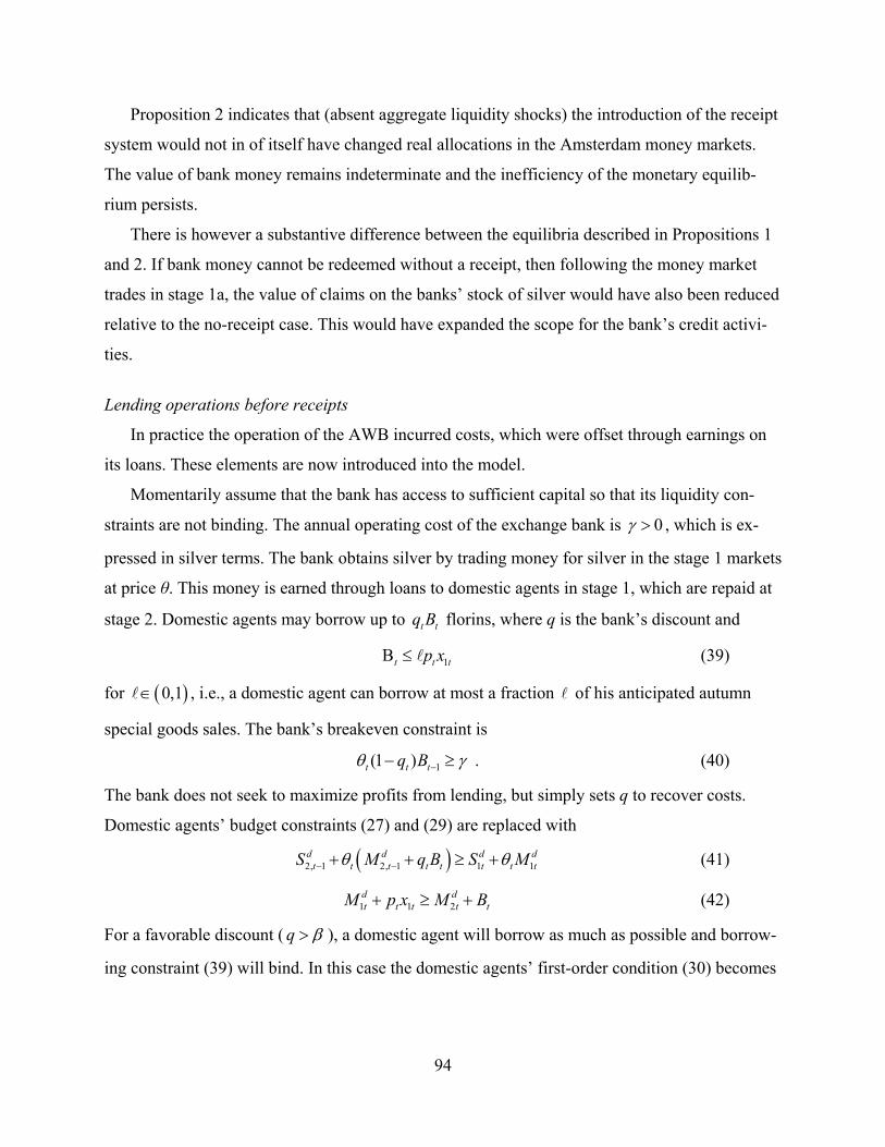
94

Proposition 2 indicates that (absent aggregate liquidity shocks) the introduction of the receipt

system would not in of itself have changed real allocations in the Amsterdam money markets.

The value of bank money remains indeterminate and the inefficiency of the monetary equilib-

rium persists.

There is however a substantive difference between the equilibria described in Propositions 1

and 2. If bank money cannot be redeemed without a receipt, then following the money market

trades in stage 1a, the value of claims on the banks’ stock of silver would have also been reduced

relative to the no-receipt case. This would have expanded the scope for the bank’s credit activi-

ties.

Lending operations before receipts

In practice the operation of the AWB incurred costs, which were offset through earnings on

its loans. These elements are now introduced into the model.

Momentarily assume that the bank has access to sufficient capital so that its liquidity con-

straints are not binding. The annual operating cost of the exchange bank is 0γ > , which is ex-

pressed in silver terms. The bank obtains silver by trading money for silver in the stage 1 markets

at price θ. This money is earned through loans to domestic agents in stage 1, which are repaid at

stage 2. Domestic agents may borrow up to t tq B florins, where q is the bank’s discount and

1t t tp xΒ ≤ (39)

for ( )0,1∈ , i.e., a domestic agent can borrow at most a fraction of his anticipated autumn

special goods sales. The bank’s breakeven constraint is

1(1 )t t tq Bθ γ−− ≥ . (40)

The bank does not seek to maximize profits from lending, but simply sets q to recover costs.

Domestic agents’ budget constraints (27) and (29) are replaced with

( )2, 1 2, 1 1 1d d d d

t t t t t t t tS M q B S Mθ θ− −+ + ≥ + (41)

1 1 2d dt t t t tM p x M B+ ≥ + (42)

For a favorable discount ( q β> ), a domestic agent will borrow as much as possible and borrow-

ing constraint (39) will bind. In this case the domestic agents’ first-order condition (30) becomes

95

[ ] ( )11

1, if (1) / *

/ * , if (1) / *

TR ax

TR a TR a

β

β β−

′ <⎧⎪= ⎨′ ′ ≥⎪⎩

(43)

where * *( ) (1 )qβ β β β= = + − > . The foreign agents’ problem does not change. Effectively,

the availability of credit lowers domestic agents’ marginal cost of producing special goods from

/a β to / *a β . An equilibrium in this case must satisfy (43) as well as the foreign agents’ first-

order condition and (24). Equilibria are described as

Proposition 3. For operating costs 0γ > sufficiently small, there is a continuum of steady-state

monetary equilibria with exchange bank lending where

(1) Allocations, the silver-equivalent price of special goods pσ θ= , and the real stock of

bank money are the same in every equilibrium;

(2) The price of money and the money price of special goods are indeterminate as in Proposi-

tion 1;

(3) The summer (end of period 1) nominal money stock varies with θ the according to

1 /M d θ= (44)

where 1d is the equilibrium consumption of the general good by domestic agents;

(4) Money is held exclusively by foreigners over the summer and domestic agents over the

winter

1 2 1; 0 ;y d dM M qB M M= + = = (45)

(5) Neither domestic nor foreign agents store silver over the winter

2 1 1 0 ;d y oS S S= = = (46)

(6) The exchange bank stores sufficient silver to satisfy its liquidity constraint (20)

( )1 2 1/ .b bS S M dδθ δ θ θ= = = (47)

Proof. Since only the domestic agents’ first-order condition (43) is modified from the previous

cases, proof is by the same arguments.

Does lending by the exchange bank improve welfare? To answer this question, one must con-

sider the capital costs of the bank’s lending program. If lending leads to an increase in consump-

96

tion by domestic agents 1d , then from (20) the bank must hold additional capital to maintain its

liquidity. As a reference case, imagine that bank’s stock of silver is obtained through a one-time,

lump-sum tax on domestic agents only.56 The following result then applies.

Corollary. The monetary equilibrium with lending is inefficient. However, for operating costs

0γ > sufficiently small, there is some equilibrium with lending that dominates the monetary

equilibrium without lending.

Proof. Inefficiency of the equilibrium with lending follows from the same arguments as in

Proposition 1.

We now compare equilibria with lending to the equilibrium without. Again two cases must

be considered. We consider the effects of a vanishingly small amount of lending (a small in-

crease in the credit limit over 0= ).

Case 1. (1) /TR a β′ < . The silver-equivalent price of special goods σ is equal to 1 for both the

equilibrium with lending and the equilibrium without. In this case, allocations are same in both

equilibria, but domestic agents produce at (effectively) a lower unit cost ( / *a β= with lending

compared to /a β without). Thus, with lending, domestic agents’ utility increases and the ex-

change bank need hold no additional silver in order to satisfy its liquidity constraint. Foreign

agents’ utility is unaffected. Hence lending dominates for this case.

Case 2. (1) /TR a β′ ≥ . The silver equivalent price of special goods σ is less than 1 in the equi-

librium without lending. Then it is straightforward to show introducing lending causes both a

decrease in σ and an increase in foreign agents’ utility.

Now consider the steady-state utility of domestic agents. Using (6) this is

1 2 (1 ) bd af Sβ− − − (48)

when the bank’s silver holdings bS are financed by a lump-sum levy on domestic agents. Using

(43) and (47) rewrite expression (48) as

( ) ( )1 11 (1 ) / [ ] ( / *) [ ] ( / *)TR TR a TR aβ δ θ θ β β− −′ ′− − −⎡ ⎤⎣ ⎦ . (49)

56 I.e., direct taxation of foreign agents is not possible. As discussed previously, in practice the bank’s capital de-rived at least partly from accumulated profits on lending. Obtaining capital in this way would have imposed addi-tional costs beyond the costs of the lump-sum levy considered here, but also would have shifted some of the bank’s capital costs to foreigners.

97

The derivative of (49) with respect to is

( ) [ ]( )2

1( ) 1 (1 ) / ** *

a aq TRβ β δ θ θ ββ β

−⎛ ⎞ ⎛ ⎞′′− − − − −⎡ ⎤⎜ ⎟ ⎜ ⎟⎣ ⎦⎝ ⎠ ⎝ ⎠

(50)

whose sign varies as the sign of

( )1 (1 ) / *β δ θ θ β− − − . (51)

As 0γ → and 1q → , (51) is positive iff

( )1 /δ θ θ− > , (52)

and, since ( )/ 1δ θ θ < , condition (52) must hold for 0> sufficiently small. In words, domestic

agents’ utility is increased if lending is slightly increased from zero. Note, however, sufficiently

large increases in lending may decrease domestic agents’ utility.

Discussion

The corollary to Proposition 3 shows that lending by the AWB could have increased welfare

even with a liquidity requirement such as (20). The need for substantial backing of bank money

would have imposed limits on the bank’s lending however. Beyond a certain point, the extra

profit obtained by increasing loans to domestic agents would have been outstripped by the atten-

dant liquidity costs. From condition (52), the liquidity constraint could have been made less

binding only by lowering either the bank’s “bid price” for bank money θ or its liquidity “com-

fort factor” δ.

From the domestic agents’ point of view, monopoly profits on sales of special goods would

have been the necessary ingredient for their support of the banks’ lending operations. With com-

petitive pricing of the special good, lending would have provided no benefit to domestic agents

and no incentive to support this activity.

Lending operations with receipts

We now consider in more detail how the introduction of receipts would have impacted the

bank’s liquidity constraints. In the pre-receipt equilibrium with lending, the year-t, beginning-of-

stage 1a (after foreign agents arrive in Amsterdam but before trading) balance sheet of the bank

is

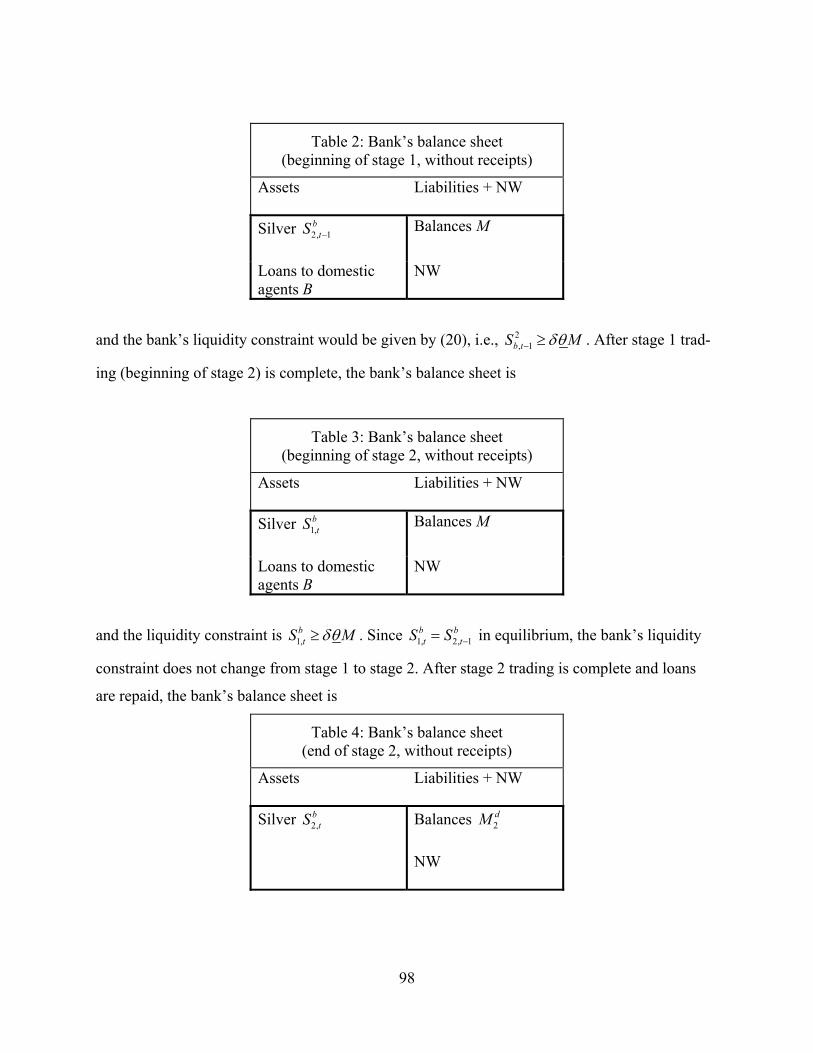
98

Table 2: Bank’s balance sheet (beginning of stage 1, without receipts)

Assets Liabilities + NW

Silver 2, 1b

tS − Balances M

Loans to domestic agents B

NW

and the bank’s liquidity constraint would be given by (20), i.e., 2, 1b tS Mδθ− ≥ . After stage 1 trad-

ing (beginning of stage 2) is complete, the bank’s balance sheet is

Table 3: Bank’s balance sheet (beginning of stage 2, without receipts)

Assets Liabilities + NW

Silver 1,btS Balances M

Loans to domestic agents B

NW

and the liquidity constraint is 1,btS Mδθ≥ . Since 1, 2, 1

b bt tS S −= in equilibrium, the bank’s liquidity

constraint does not change from stage 1 to stage 2. After stage 2 trading is complete and loans

are repaid, the bank’s balance sheet is

Table 4: Bank’s balance sheet (end of stage 2, without receipts)

Assets Liabilities + NW

Silver 2,b

tS Balances 2dM

NW

99

The liquidity constraint at this stage is 2, 2b d

tS Mδθ≥ , which, since 2, 1,b b

t tS S= in equilibrium, is

implied by the previous liquidity constraints.

Now consider the bank’s balance sheets at the same stages under the receipt system. At the

beginning of money market trading stage 1a, the bank’s balance sheet is

Table 5: Bank’s balance sheet (beginning of stage 1, with receipts)

Assets Liabilities + NW

Silver 2, 1 1b

tS D− +

Loans to domestic agents B

Balances M of domestic agents

Balances 1D of foreign agents [of which 1D redeemable on demand]

NW

If the bank is only committed to pay coin against all outstanding receipts, its liquidity constraint

is

2, 1 1 1 1 1b

tS D L D L− + − ≥ − (53)

or simply

2, 1 1 0btS L− + ≥ . (54)

Following stage 1 trading, the bank’s balance sheet is

Table 6: Bank’s balance sheet (beginning of stage 2, with receipts)

Assets Liabilities + NW

Silver 1, 2, 1 1 1b bt tS S D L−= + −

Loans to domestic agents B

Balances 1 1D Lλ+ of foreign agents [ 1 1D L− redeemable on demand]

NW

If the bank is committed to pay coin against all outstanding receipts, its liquidity constraint is

100

2, 1 1 1 1 1b

tS D L D L− + − ≥ − (55)

or

2, 1 0btS − ≥ (56)

Finally, after stage 2 trading is complete, the bank’s balance sheet contracts to

Table 7: Bank’s balance sheet (end of stage 2, with receipts)

Assets Liabilities + NW

Silver 2, 2, 1b b

t tS S −= Balances 2dM

NW

Since all receipts have been redeemed by this point, there is no liquidity constraint on the bank.

To summarize, these calculations indicate that under the receipt system, an expansion of the

bank’s lending B need not be backed by an expansion of its silver holdings bS , essentially be-

cause, under receipts, the bank’s liquidity constraint is slackened from (47) (in its equilibrium

form) to (56). Indeed, in the steady-state world analyzed here, it is conceivable that the bank

holds no silver over the winter. To avoid indeterminacy of the silver price of money θ in particu-

lar, however, we assume that the bank must commit (off-equilibrium) to sell silver (i.e., receipts)

at its target price, and possess “enough” silver 0S > to back this pledge.

This does not explain how large S must be to guarantee determinacy. As a benchmark for

the comparisons below, we take S to be the value of 2bS necessary to support the monetary equi-

librium without lending, i.e., 2bS S= as specified in (35).

Our last set of results confirms agents’ preferences for the receipts arrangement:

Proposition 4. With receipts, the monetary equilibrium with lending is identical to the equilib-

rium given in Proposition 3, except that the bank’s winter silver stock 2bS is reduced to S .

Proof. As in Proposition 2, optimality conditions and market clearing are not affected by the in-

troduction of receipts.

101

Corollary 1. For a given credit limit parameter , the equilibrium with receipts dominates the

equilibrium without receipts.

Proof. Decreasing the bank’s winter silver holdings (as occurs with the introduction of receipts)

does not change allocations of consumption goods, and lowers the deadweight loss.

Corollary 2. Under receipts, welfare is increasing in .

Proof. With receipts, an expansion of lending does not result in an increase in the bank’s win-

ter silver holdings 2bS . From (47), the bank’s summer silver stock 1

bS increases but this is occurs

through voluntary deposits by foreign agents; domestic agents bear no additional liquidity cost.

Hence this cost does not enter into welfare comparisons.

Increasing increases domestic agents’ welfare increases because, from (43), this lowers

their marginal costs of production, while their marginal revenue from special good sales remains

the same.

Foreign agents’ welfare increases as in Proposition 3; hence, total welfare increases.