Statistics of ‘‘Synoptic Circulation Weather’’ in the North Sea as Derived from a Multiannual OGCM Simulation

DECEMBER 2000 3039K A U K E R A N D V O N S T O R C H

q 2000 American Meteorological Society

Statistics of ‘‘Synoptic Circulation Weather’’ in the North Sea asDerived from a Multiannual OGCM Simulation

FRANK KAUKER AND HANS VON STORCH

Institute of Hydrophysics, GKSS Research Centre, Geesthacht, Germany

(Manuscript received 22 February 1999, in final form 14 January 2000)

ABSTRACT

A 15-yr simulation of an ocean general circulation model, exposed to atmospheric forcing as provided by theECMWF reanalysis 1979–93, is analyzed with respect to the statistics of the surface circulation of the NorthSea on timescales of days to several weeks in winter.

The first two EOFs of surface circulation are found to represent the bulk of the variability (72%). They arebroadly consistent with the limited observational record. The first EOF represents regimes with one gyre flushingthe entire North Sea, either with clockwise orientation (15% of time) or with counterclockwise orientation (30%of time). These regimes are excited by northeasterly and, respectively, southwesterly wind. The second EOF isrepresentative for two opposite regimes with two bipolar patterns in the northern and southern part of the NorthSea (45% of time). For a certain range of both EOFs coefficients, the North Sea circulation ceases (10% oftime).

The circulation of the North Sea in winter is highly variable; the regimes change frequently. Only 40% ofthe one-gyre regimes persist for longer than 5 days, and the bipolar pattern regimes rarely extend for more than5 days.

1. Introduction

The North Sea as a dynamical system attracts ourinterest for various reasons. This interest is partly re-flecting our scientific curiosity, and is partly due to theimportance of the North Sea for various socioeconomicaspects, ranging from fisheries, the transport of matter,and more generally, water quality. For these purposes,we are in need of reliable information about the dy-namical state of the North Sea; we need to know therange of natural variability in terms of phenomena, in-tensity, and temporal and spatial extension.

The dynamics of the oceans as well as the atmosphereis characterized by the presence of infinitely many pro-cesses operating on a wide range of spatial and temporalscales. Therefore, mapping the instantaneous state ofthe oceans, or the atmosphere, is far from trivial, andcan hardly be done from observations alone. This taskis particularly demanding for the oceans, where obser-vations of the dynamical state—for instance, currentsor stream function—require costly in situ operations.Because of this limitation, the international oceano-graphic community has embarked on the challenging

Corresponding author address: Frank Kauker, Alfred-Wegener-In-stitute for Polar and Marine Research, P.O. Box 12 01 61, D-27515Bremerhaven, Germany.E-mail: [email protected]

undertaking of ‘‘operational oceanography,’’ which bymeans of intelligent merging of dynamical understand-ing (i.e., quasi-realistic models), of educated guessing(i.e., routine forecasts), and routine in situ and remotelysensed observations of a wide range of variables allowsfor a instantaneous, synoptic analysis of the state of theocean (Robinson et al. 1998). These endeavors are pur-sued under the umbrella of international projects suchas GOOS and EUROGOOS.

Currently, multiyear time series of regularly preparedanalyses of the state of the North Sea are available onlyfor variables such as sea surface temperature (Beckerand Pauly 1996) and coastal sea level at various tidestations. For circulation, such analyses are unavailablefor an extented time period suitable for a statistical anal-ysis of inter- and intradecadal variability. Instead, epi-sodic data at selected vertical profiles and cross sectionshad to be relied upon (see, e.g., Furnes 1980 or Sun-dermann 1994). Numerical models have been appliedto investigate the dependence of the circulation on thestrength and direction of the wind (Backhaus 1993;Backhaus and Hainbucher 1987; Maier-Reimer 1975),but this kind of sensitivity studies does not give insightsinto the statistics of the circulation. Additionally, mul-tiyear simulations (Langenberg et al. 1999; Flather etal. 1998; Smith et al. 1996; Pohlmann 1996) have beenexecuted, which provide an educated guess of the tem-poral and spatial variability of the dynamical state. Un-fortunately, these long-term integrations have not been

3040 VOLUME 30J O U R N A L O F P H Y S I C A L O C E A N O G R A P H Y

analyzed with respect to the statistics of synoptic var-iability of the circulation. Also, they partially sufferfrom inhomogeneities in the atmospheric forcing fields.

We used a full-fledged ocean general circulation mod-el—Oberhuber’s (1993) isopycnical GCM—adapted tothe particular situation of the North Sea and the neigh-boring shelf ocean [for details, refer to Kauker and Ob-erhuber (1997) and Kauker (1999)] forced with the ho-mogeneous meteorological reanalysis provided byECMWF (1979–93). The model, the forcing data, andthe simulation are summarized in section 2. The skillof the model in reproducing observational evidence hasbeen assessed by Kauker (1999); therefore, we limitourselves to a few comparisons of simulated and ‘‘ob-served’’ data.

The simulated distributions of horizontal streamfunc-tion at the surface was stored on a daily basis togetherwith many other variables. In the present paper we an-alyze these data with the intention to identify and char-acterize circulation regimes (section 3). The analysismakes use of the standard multivariate technique of Em-pirical Orthogonal Functions or Principal Components(von Storch and Frankignoul 1998). The first two EOFsturn out to represent most of the large-scale variabilityof the North Sea circulation. This inspires the projectionof the state of the North Sea onto the two-dimensionalphase space spanned by the first two EOFs. Then, dif-ferent parts of this 2D phase space are identified withdifferent regimes. They are characterized by the cir-culation, the simultaneous air pressure fields, their res-idence time distributions, and probabilities for transfersbetween the regimes. Evidence from the observationalrecord is compared with model results in section 4. Inthe concluding section 5 the results are related to hy-potheses available from the literature, and a short gen-eral discussion of the value and limitation of using out-put from quasi-realistic ocean models as a substitute forobservational data is offered.

2. OGCM, data

The regional Ocean isoPYCnic (OPYC) model (Kau-ker and Oberhuber 1997) is a derivative of Oberhuber’sOPYC model, which has been found to be a flexibleand reliable simulation tool by a variety of researchers(e.g., Miller et al. 1994; Holland et al. 1996; Lunkeitet al. 1996; Cabos Narvaez et al. 1998; Junge et al.2000). In the present application, the model was adaptedfor describing variations of sea level, temperature, andsalinity in the North Sea. Also the influence of the stateof the adjacent oceans was to be studied. Therefore, theNorth Sea and the adjacent Northeast Atlantic as wellas the Norwegian–Iceland–Greenland Seas (GIN Seas)is modeled. The model area is rotated and approximatelygiven by the following four corners (37849N, 38499W),(448449N, 29809E), (618499N, 298119W), and (808139N,258449W). The horizontal resolution varies from ½8 3½8 at the lateral boundaries to 69 3 69 in the central

North Sea. The topmost layer is formulated as a mixedlayer. The deeper ocean is discretized in the verticalwith 14 Lagrangian isopycnal layers. The three-dimen-sional OPYC model solves the primitive equation witha time step of 3 h, that is, solves the slow barotropicand baroclinic modes. A barotropic tide model, whichsolves the faster tidal modes, is coupled to the 3D model.The four strongest partial tides are prescribed at thelateral boundaries of the tide model. The 3D model iscoupled to the tide model via the bottom stress and theresidual circulation of the tide model.

The density varies according to advection of tem-perature and salinity as well as surface fluxes. An annualmean flux adjustment for heat and freshwater is appliedin the Northeast Atlantic and the GIN Seas, but not forthe North Sea. The freshwater input from the rivers iscalculated with the help of a soil model and a dischargemodel.

The regional OPYC model is forced with surface datafrom the European Centre of Medium-Range WeatherForecasts (ECMWF) reanalysis project (Gibson et al.1997). The data of the operational weather model of theECMWF have the disadvantage that over time theweather model was continuously changed with respectto resolution and to parameterizations of subgrid scaleprocesses. Also, the initialization scheme was contin-uously updated. In 1993, the ECMWF decided to hind-cast the time period 1979 to 1993 with a fixed setup,that is, with a fixed weather forecast model and a fixeddata assimilation scheme. The selected weather modelhas a T106 horizontal resolution and 31 vertical layers.With the help of the data assimilation scheme, the op-timal initial values are calculated. Here, the 12-hourlyforecasts are used as forcing data for the regional OPYCmodel.

The advantage of the ECMWF reanalyses is their ho-mogeneity: the weather model and the assimilationscheme are fixed and the output is dynamically consis-tent; that is, all variables are related via the underlyingrealizations of the physical processes of the weathermodel.

The heat and freshwater fluxes are calculated fromthe regional OPYC model in dependence of the 2-m airtemperature, SST, dewpoint temperature, cloudiness,and precipitation. The solar radiation and the wind stressare taken from the reanalysis directly.

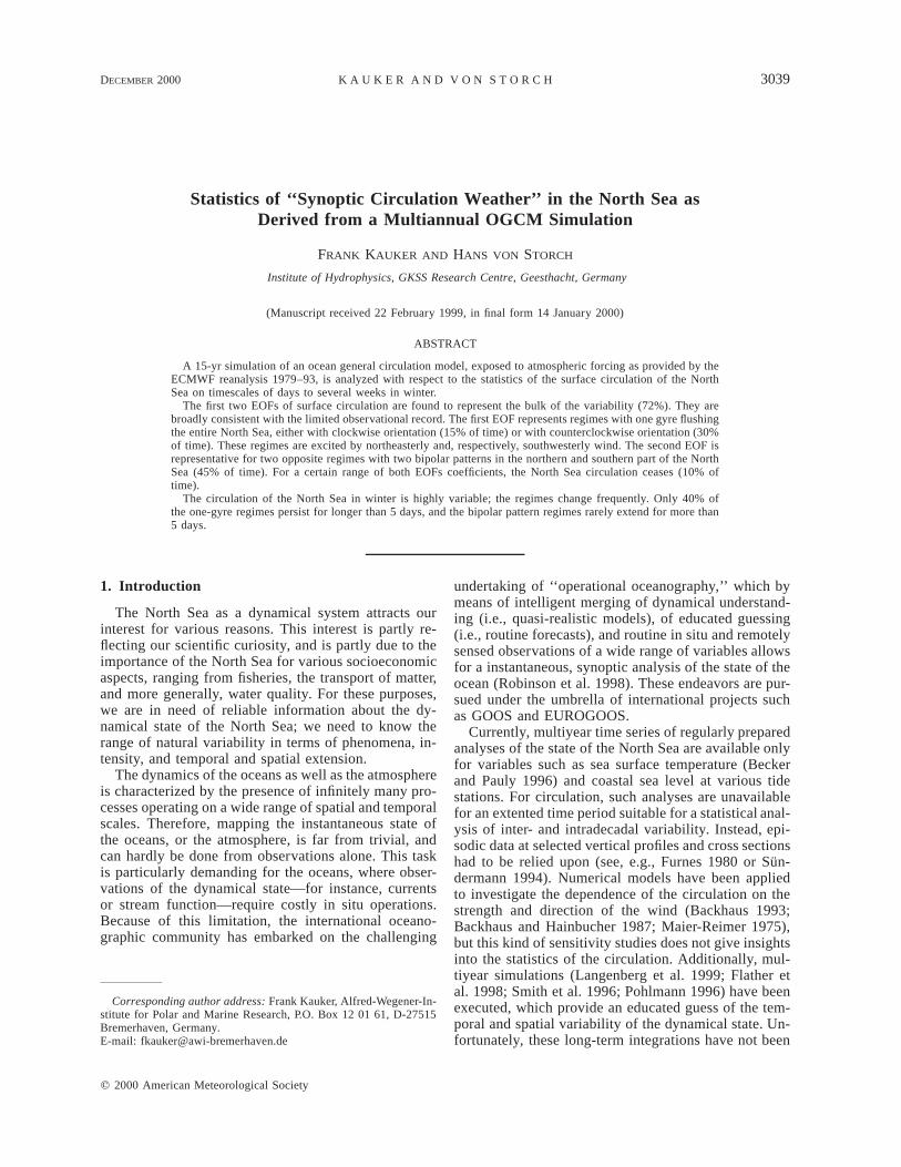
The skill of the model in reproducing ‘‘observed’’features is demonstrated here by showing the winter-mean horizontal surface streamfunction (Fig. 1), and bycomparing times series of sea level at Esbjerg (at theDanish coast of the North Sea, Fig. 2) and of the dis-tribution of simulated and analyzed surface salinity con-centrations in February 1982 (Fig. 3). For a more de-tailed validation of the model we refer to Kauker (1999).

The simulated winter (Dec, Jan, and Feb) mean cir-culation (Fig. 1) is organized in one counterclockwisegyre, flushing the entire North Sea in about 650 dayswith typical mean velocities of 10 cm s21. It compares

DECEMBER 2000 3041K A U K E R A N D V O N S T O R C H

FIG. 1. Time mean horizontal surface velocity stream function Cin winter (Dec, Jan, and Feb). Negative values are shaded. The min-imum describes a basinwide, counterclockwise circulation with aninflow in the west and an outflow in the east. The Greenwich meridianand the 608N latitude line are shown to help with geographical ori-entation.

well with estimates derived from observations (Svend-sen et al. 1995).

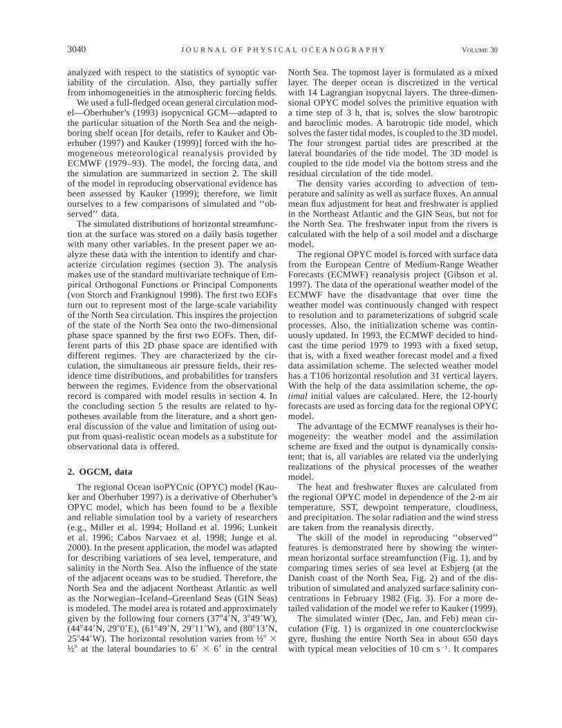
The observed time series of sea level variations atEsbjerg are well reproduced by the model (Fig. 2) as isdemonstrated by the similarity of the autospectra, aphase lag close to zero for all frequencies and the highsquared coherency. Only for timescales shorter than,say, 2 days the power of the simulated auto spectrumfalls off, and the coherency becomes notably smaller.This is not surprising as the model was constructed tosimulate variations on timescales longer than several M2

tides. As sketched above, the effect of the tides is in-cluded only in parameterized form.

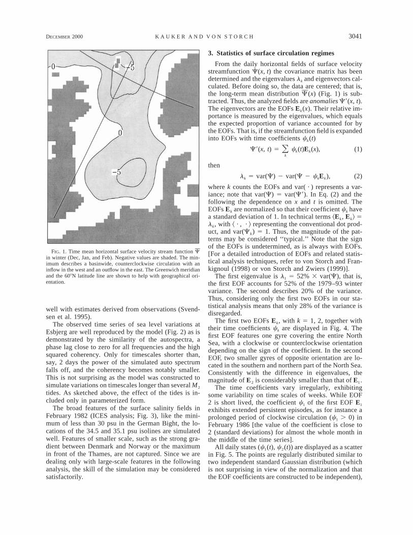
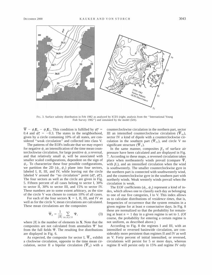
The broad features of the surface salinity fields inFebruary 1982 (ICES analysis; Fig. 3), like the mini-mum of less than 30 psu in the German Bight, the lo-cations of the 34.5 and 35.1 psu isolines are simulatedwell. Features of smaller scale, such as the strong gra-dient between Denmark and Norway or the maximumin front of the Thames, are not captured. Since we aredealing only with large-scale features in the followinganalysis, the skill of the simulation may be consideredsatisfactorily.

3. Statistics of surface circulation regimes

From the daily horizontal fields of surface velocitystreamfunction C(x, t) the covariance matrix has beendetermined and the eigenvalues lk and eigenvectors cal-culated. Before doing so, the data are centered; that is,the long-term mean distribution C(x) (Fig. 1) is sub-tracted. Thus, the analyzed fields are anomalies C9(x, t).The eigenvectors are the EOFs Ek(x). Their relative im-portance is measured by the eigenvalues, which equalsthe expected proportion of variance accounted for bythe EOFs. That is, if the streamfunction field is expandedinto EOFs with time coefficients ck(t)

C9(x, t) 5 c (t)E (x), (1)O k kk

then

lk 5 var(C) 2 var(C 2 ckEk), (2)

where k counts the EOFs and var( · ) represents a var-iance; note that var(C) 5 var(C9). In Eq. (2) and thefollowing the dependence on x and t is omitted. TheEOFs Ek are normalized so that their coefficient ck havea standard deviation of 1. In technical terms ^Ek, Ek& 5lk, with ^ · , · & representing the conventional dot prod-uct, and var(Ck) 5 1. Thus, the magnitude of the pat-terns may be considered ‘‘typical.’’ Note that the signof the EOFs is undetermined, as is always with EOFs.[For a detailed introduction of EOFs and related statis-tical analysis techniques, refer to von Storch and Fran-kignoul (1998) or von Storch and Zwiers (1999)].

The first eigenvalue is l1 5 52% 3 var(C), that is,the first EOF accounts for 52% of the 1979–93 wintervariance. The second describes 20% of the variance.Thus, considering only the first two EOFs in our sta-tistical analysis means that only 28% of the variance isdisregarded.

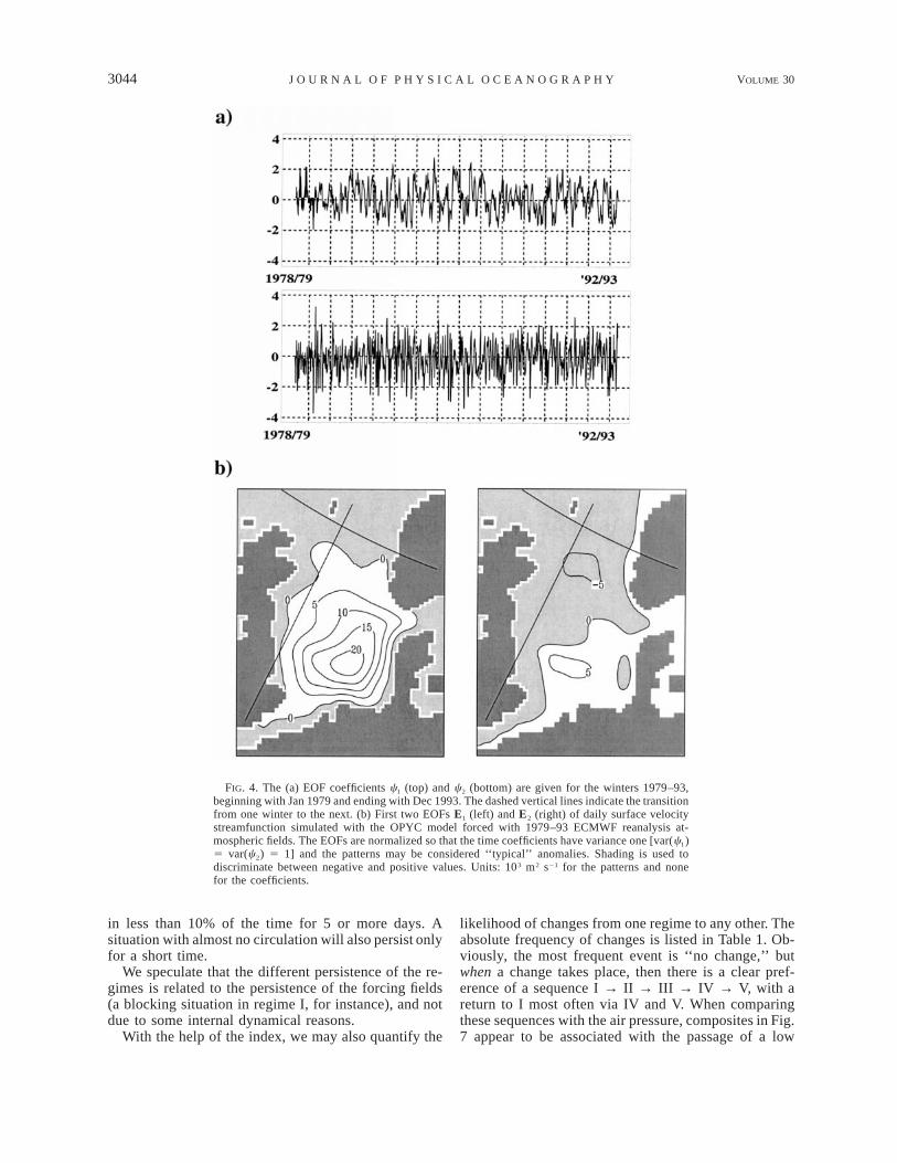
The first two EOFs Ek, with k 5 1, 2, together withtheir time coefficients ck are displayed in Fig. 4. Thefirst EOF features one gyre covering the entire NorthSea, with a clockwise or counterclockwise orientationdepending on the sign of the coefficient. In the secondEOF, two smaller gyres of opposite orientation are lo-cated in the southern and northern part of the North Sea.Consistently with the difference in eigenvalues, themagnitude of E2 is considerably smaller than that of E1.

The time coefficients vary irregularly, exhibitingsome variability on time scales of weeks. While EOF2 is short lived, the coefficient c1 of the first EOF E1

exhibits extended persistent episodes, as for instance aprolonged period of clockwise circulation (c1 . 0) inFebruary 1986 [the value of the coefficient is close to2 (standard deviations) for almost the whole month inthe middle of the time series].

All daily states (c1(t), c2(t)) are displayed as a scatterin Fig. 5. The points are regularly distributed similar totwo independent standard Gaussian distribution (whichis not surprising in view of the normalization and thatthe EOF coefficients are constructed to be independent),

3042 VOLUME 30J O U R N A L O F P H Y S I C A L O C E A N O G R A P H Y

FIG. 2. Spectral analysis of simulated and observed sea level variations at Esbjerg (Denmark).(a) Autospectra: A represents the simulated data, B the observed data. (b) Phase spectrum: positiveangles indicate that the simulated data lead the observed data, and negative angles that theobservations lead the simulation. (c) Squared coherency spectrum: the dashed limits are thresh-olds, allowing to reject the null hypothesis of zero coherency with a risk of 90%, 95%, and 99%.

even though there is an indication that the distributionof c1 (along the horizontal axis) may be a bit skewedto the right. A visual inspection of Fig. 5 reveals nofurther structure in the scatter ; this finding is substan-tiated by a cluster analysis that returned no meaningfulpartitioning of the scatter.

The EOF coefficient time series ck are used to definethe regimes. For that purpose, first that pair of coeffi-cients ( , ) is determined such that the reconstruc-c* c*1 2

tion E1 1 E2 represents a state with almost noc* c*1 2

circulation. The ‘‘no circulation’’ point ( , ) is foundc* c*1 2

by minimizing the area-averaged standard deviation of

DECEMBER 2000 3043K A U K E R A N D V O N S T O R C H

FIG. 3. Surface salinity distribution in Feb 1982 as analyzed by ICES (right; analysis from the ‘‘International YoungFish Survey 1982’’) and simulated by the model (left).

C 2 c1E1 2 c2E2. This condition is fulfilled by 5c*10.4 and 5 20.3. The states in the neighborhood,c*2given by a circle containing 10% of all states, are con-sidered ‘‘weak circulation’’ and collected into class V.

The patterns of the EOFs indicate that we may expectfor negative c1 an intensification of the time mean coun-terclockwise circulation, for large positive c1 a reversal,and that relatively small c1 will be associated withsmaller scaled configurations, dependent on the sign ofc2. To characterize these four possible configurations,we partition the 2D (c1, c2) plane into four sectors,labeled I, II, III, and IV, while leaving out the circlelabeled V around the ‘‘no circulation’’ point ( , ).c* c*1 2

The four sectors as well as the circle are given in Fig.5. Fifteen percent of all cases belong to sector I, 30%to sector II, 30% to sector III, and 15% to sector IV.These numbers are to some extent arbitrary, as the sizeof the circle V was chosen to contain 10% of all cases.

For each of the four sectors X 5 I, II, III, and IV aswell as for the circle V, mean circulations are calculated.These mean circulations are the composites

1C 5 C, (3)OX |X| (c ,c )∈X1 2

where |X| is the number of elements in X. Note that thecomposites are not calculated from anomalies C9 butfrom the full fields C. The resulting five distributionsare displayed in Fig. 6.

As expected, the composite for sector I, C I , exhibita clockwise circulation, opposite to the time mean cir-culation, sector II a bipolar circulation (C II) with a

counterclockwise circulation in the northern part, sectorIII an intensified counterclockwise circulation (C III),sector IV a kind of dipole with a counterclockwise cir-culation in the southern part (C IV), and circle V nosignificant structure (CV).

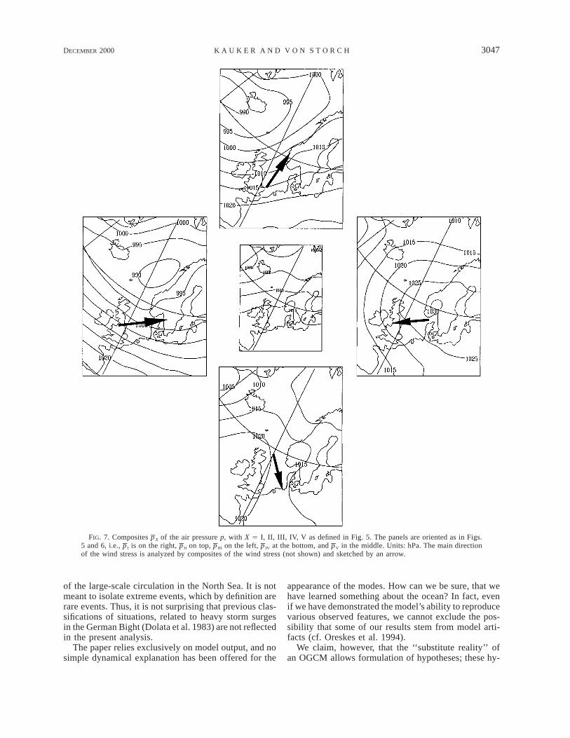
In the same manner, composites p X of surface airpressure have been calculated and are displayed in Fig.7. According to these maps, a reversed circulation takesplace when northeasterly winds prevail (compare C I

with p I), and an intensified circulation when the windis southwesterly. The smaller counterclockwise gyre inthe northern part is connected with southwesterly wind,and the counterclockwise gyre in the southern part withnortherly winds. Weak westerly winds prevail when thecirculation is weak.

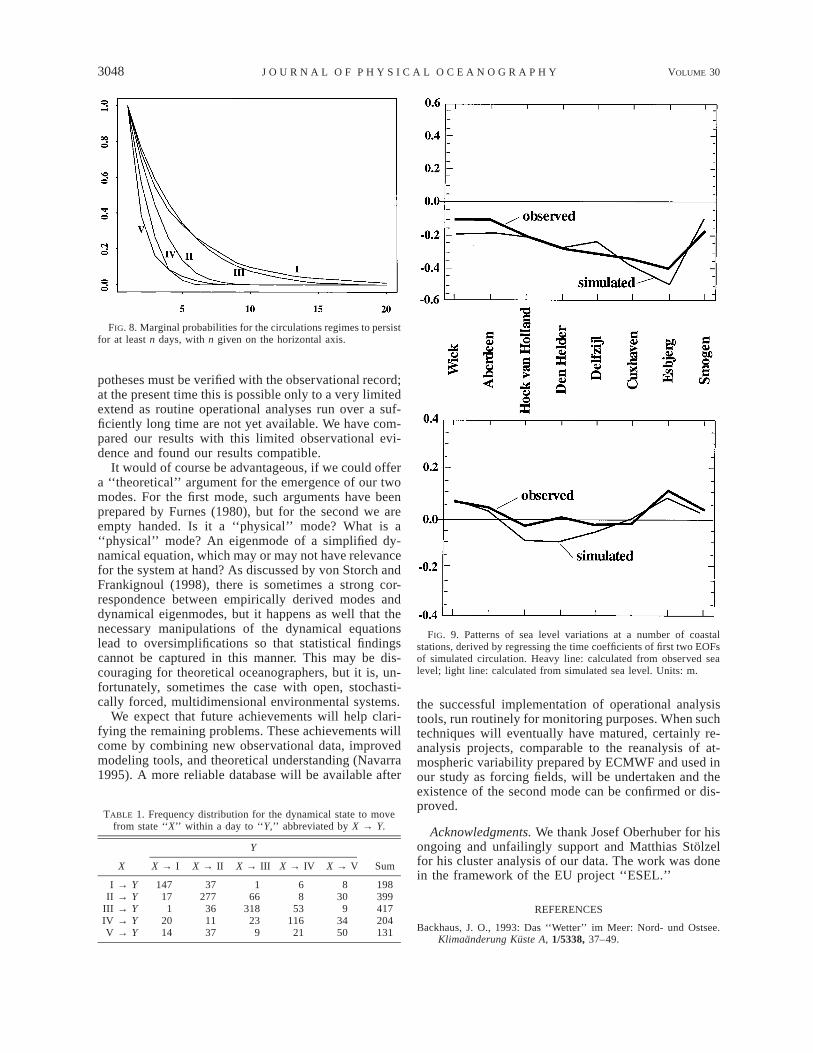
The EOF coefficients (c1, c2) represent a kind of in-dex, which allows one to classify each day as belongingto one of our five categories, I to V. This index allowsus to calculate distributions of residence times, that is,frequencies of occurrence that the system remains in agiven regime for at least n consectutive days. In Fig. 8these are normalized so that the probability for remain-ing at least n 5 1 day in a given regime is set to 1. (Ofcourse, the probability for entering a certain regime isnot uniform, as described above.)

According to Fig. 8 the regimes I and III, with anintensified or reversed basinwide circulation, are con-siderably more persistent than regimes II and IV as wellas V. Forty percent of initial intensified, or reversed,circulations will persist for 5 or more days, whereasregime II will persist only in 15% and regime IV only

3044 VOLUME 30J O U R N A L O F P H Y S I C A L O C E A N O G R A P H Y

FIG. 4. The (a) EOF coefficients c1 (top) and c2 (bottom) are given for the winters 1979–93,beginning with Jan 1979 and ending with Dec 1993. The dashed vertical lines indicate the transitionfrom one winter to the next. (b) First two EOFs E1 (left) and E2 (right) of daily surface velocitystreamfunction simulated with the OPYC model forced with 1979–93 ECMWF reanalysis at-mospheric fields. The EOFs are normalized so that the time coefficients have variance one [var(c1)5 var(c2) 5 1] and the patterns may be considered ‘‘typical’’ anomalies. Shading is used todiscriminate between negative and positive values. Units: 103 m2 s21 for the patterns and nonefor the coefficients.

in less than 10% of the time for 5 or more days. Asituation with almost no circulation will also persist onlyfor a short time.

We speculate that the different persistence of the re-gimes is related to the persistence of the forcing fields(a blocking situation in regime I, for instance), and notdue to some internal dynamical reasons.

With the help of the index, we may also quantify the

likelihood of changes from one regime to any other. Theabsolute frequency of changes is listed in Table 1. Ob-viously, the most frequent event is ‘‘no change,’’ butwhen a change takes place, then there is a clear pref-erence of a sequence I → II → III → IV → V, with areturn to I most often via IV and V. When comparingthese sequences with the air pressure, composites in Fig.7 appear to be associated with the passage of a low

DECEMBER 2000 3045K A U K E R A N D V O N S T O R C H

FIG. 5. Scatter diagram of the coefficients of the first two EOFs ofNorth Sea surface velocity streamfunction. The horizontal axis rep-resents the first coefficients and the vertical axis the second. Thediagonal cross represents a partitioning of the 2D phase space, withthe circle around the origin of this cross representing states with weakoverall circulation. The four areas, labeled I, II, III, and IV, and thecircle V, are discussed in the text. The time mean state correspondingto zero EOF coefficients is depicted in Fig. 1.

pressure system in easterly direction across the NorthSea.

4. Consistency with the observed sea level record

The question arises whether the two modes found inthe multiyear simulation are consistent with the obser-vational record. As mentioned in the introduction, adirect comparison with ‘‘observed’’ circulation data isimpossible for the time being since multiyear analysesof circulation are unavailable. Furthermore the com-parison with data from spatially and temporarily limitedobservational campaigns is inconclusive. For instance,the Furnes (1980) analysis of data collected duringJONSDAP 1976 covers only 2 months of observationson a cross section between Scotland and Norway. Allthat can be said is that our first mode is consistent withhis findings. But what about the second mode?

The only extended, homogeneous dataset available issea level recorded at a number of tide gauges along thecoast. We had the data from Wick, Aberdeen (UK),Hoek van Holland, Den Helder, Delfzijl (NL), Cuxhaven(D), Esbjerg (DK), and Smogen (S) at our disposal.

We regressed the coefficients c1 and c2 of the firsttwo circulation EOFs (Fig. 4) on the sea level variationszj(t) at the j 5 1, . . . , 8 gauges along the North Seacoast; that is, we determined numbers g i,j such that

2(c (t) 2 g z (t)) 5 min. (4)O i i, j jt

We used both observed and simulated sea level varia-tions. The resulting numbers g i,j are displayed as curvesin Fig. 9. Keeping in mind that the tide gauges reflectto some extent local effects unknown to the dynamicalmodel, the similarity between the regression coefficientsfor the observed and simulated sea level variations isremarkable for both EOFs.

The projection of the first EOF (Fig. 4) on the coastalsea level reveals a general lowering of the water level,of the order of 20 to 40 cm. This lowering is consistentwith the anomalous counterclockwise circulation, withstrongest gradients off the Danish coast (i.e., Esbjerg)and weakest gradients along the Scottish coast (Wick,Aberdeen). The argument is linear so that a negativeEOF coefficient c1(t) is associated with higher sea levelsalong the coasts.

The second EOF (Fig. 4) is composed of smaller-scaled features; these are reflected in the regression co-efficients. The minima in streamfunction, located off theScottish and the Danish coast, represent clockwise cir-culations and are consistently associated with an in-crease of coastal sea level (of the order of 10 cm), where-as in the southern North Sea an anomalous counter-clockwise circulation prevails. Consistently, the sea lev-el anomalies are negative along the Dutch and Germancoast.

That the OGCM generates a dynamically consistentlink between the circulation patterns and coastal sealevel variations is not surprising, as the model has beenconstructed to be dynamically consistent. However, thatsimilar patterns emerge from the observational recordis not trivial; indeed, this is a strong support for thereality of both EOF patterns.

5. Conclusions

The results of the present study may be summarizedas follows.

1) The statistics of large-scale surface circulation of theNorth Sea is a two-dimensional phenomenon andmay be described by the first two EOFs. Both EOFsare found compatible with the observational record.

2) With the help of the first two EOFs a set of fourregimes may be defined, which differ in their dy-namical characteristics. The regimes change fre-quently, only about 20% of a regime persists formore than 5 days. That is, the North Sea circulationis highly variable with characteristic times of a fewdays.

3) Two regimes, associated with EOF 1 of the surfacevelocity streamfunction, exhibit one basinwide gyre,with an intensified time mean circulation or a re-versed time mean circulation. The former is linkedto southwesterly winds and prevails about one-thirdof the time, whereas the latter is linked to north-easterly winds and appears 15% of the time. Bothregimes persist 40% of the time for 5 days or longer.

3046 VOLUME 30J O U R N A L O F P H Y S I C A L O C E A N O G R A P H Y

FIG. 6. Composites C X of the surface velocity stream function C, with X 5 I, II, III, IV, V as defined in Fig. 5. The panelsare oriented as in Fig. 5, i.e., C I is on the right, C II on top, C III on the left, C IV at the bottom, and CV in the middle. Negativevalues are shaded. Units: 103 m2 s21.

4) Two other regimes, associated with EOF 2, exhibita bipolar pattern with opposite gyres in the northernand southern part of the North Sea. These structuresare connected with southerly and northerly windsand are short lived. The southerly wind regime per-sists for 5 or more days 20% of the time, whereasthe northerly wind regime persists for 5 or more daysonly 5% of the time.

5) The regimes often undergo a sequence, which is

characteristic for the passage of a low pressure sys-tem across the North Sea.

The results are qualitatively in accord with the hy-potheses of Furnes (1980) and Backhaus (1993), evenif certain aspects, such as the characteristic wind direc-tions associated with the different ‘‘circulation re-gimes,’’ deviate somewhat from Backhaus’ hypothesis.

The present analysis is meant to describe the statistics

DECEMBER 2000 3047K A U K E R A N D V O N S T O R C H

FIG. 7. Composites p X of the air pressure p, with X 5 I, II, III, IV, V as defined in Fig. 5. The panels are oriented as in Figs.5 and 6, i.e., p I is on the right, p II on top, p III on the left, p IV at the bottom, and p V in the middle. Units: hPa. The main directionof the wind stress is analyzed by composites of the wind stress (not shown) and sketched by an arrow.

of the large-scale circulation in the North Sea. It is notmeant to isolate extreme events, which by definition arerare events. Thus, it is not surprising that previous clas-sifications of situations, related to heavy storm surgesin the German Bight (Dolata et al. 1983) are not reflectedin the present analysis.

The paper relies exclusively on model output, and nosimple dynamical explanation has been offered for the

appearance of the modes. How can we be sure, that wehave learned something about the ocean? In fact, evenif we have demonstrated the model’s ability to reproducevarious observed features, we cannot exclude the pos-sibility that some of our results stem from model arti-facts (cf. Oreskes et al. 1994).

We claim, however, that the ‘‘substitute reality’’ ofan OGCM allows formulation of hypotheses; these hy-

3048 VOLUME 30J O U R N A L O F P H Y S I C A L O C E A N O G R A P H Y

FIG. 8. Marginal probabilities for the circulations regimes to persistfor at least n days, with n given on the horizontal axis.

FIG. 9. Patterns of sea level variations at a number of coastalstations, derived by regressing the time coefficients of first two EOFsof simulated circulation. Heavy line: calculated from observed sealevel; light line: calculated from simulated sea level. Units: m.

TABLE 1. Frequency distribution for the dynamical state to movefrom state ‘‘X’’ within a day to ‘‘Y,’’ abbreviated by X → Y.

X

Y

X → I X → II X → III X → IV X → V Sum

I → YII → Y

III → YIV → YV → Y

14717

12014

37277

361137

166

31823

9

68

53116

21

830

93450

198399417204131

potheses must be verified with the observational record;at the present time this is possible only to a very limitedextend as routine operational analyses run over a suf-ficiently long time are not yet available. We have com-pared our results with this limited observational evi-dence and found our results compatible.

It would of course be advantageous, if we could offera ‘‘theoretical’’ argument for the emergence of our twomodes. For the first mode, such arguments have beenprepared by Furnes (1980), but for the second we areempty handed. Is it a ‘‘physical’’ mode? What is a‘‘physical’’ mode? An eigenmode of a simplified dy-namical equation, which may or may not have relevancefor the system at hand? As discussed by von Storch andFrankignoul (1998), there is sometimes a strong cor-respondence between empirically derived modes anddynamical eigenmodes, but it happens as well that thenecessary manipulations of the dynamical equationslead to oversimplifications so that statistical findingscannot be captured in this manner. This may be dis-couraging for theoretical oceanographers, but it is, un-fortunately, sometimes the case with open, stochasti-cally forced, multidimensional environmental systems.

We expect that future achievements will help clari-fying the remaining problems. These achievements willcome by combining new observational data, improvedmodeling tools, and theoretical understanding (Navarra1995). A more reliable database will be available after

the successful implementation of operational analysistools, run routinely for monitoring purposes. When suchtechniques will eventually have matured, certainly re-analysis projects, comparable to the reanalysis of at-mospheric variability prepared by ECMWF and used inour study as forcing fields, will be undertaken and theexistence of the second mode can be confirmed or dis-proved.

Acknowledgments. We thank Josef Oberhuber for hisongoing and unfailingly support and Matthias Stolzelfor his cluster analysis of our data. The work was donein the framework of the EU project ‘‘ESEL.’’

REFERENCES

Backhaus, J. O., 1993: Das ‘‘Wetter’’ im Meer: Nord- und Ostsee.Klimaanderung Kuste A, 1/5338, 37–49.

DECEMBER 2000 3049K A U K E R A N D V O N S T O R C H

, and D. Hainbucher, 1987: A finite difference general circulationmodel for shelf seas and its application to low frequency vari-ability on the north European Shelf. Three-Dimensional Modelsof Marine and Estuarine Dynamics, J. C. J. Nihoul and B. M.Jamart, Eds., Elsevier, 221–224.

Becker, G. A., and M. Pauly, 1996: Sea surface temperature changesin the North Sea and their causes. J. Mar. Sci., 53, 887–898.

Cabos Narvaez, W., M. J. Ortiz Bevia, and J. M. Oberhuber, 1998:The variability of the tropical Atlantic. J. Geophys. Res., 103C,7475–7489.

Dolata, L. F., E. Roeckner, and H. Behr, 1983: Prognostic storm surgesimulation with a combined meteorological/oceanographic mod-el. North Sea Dynamics, J. Sundermann and W. Lenz, Eds.,Springer-Verlag, 266–278.

Flather, R. A., J. A. Smith, J. D. Richards, C. Bell, and D. L. Black-man, 1998: Direct estimates of extreme storm surge elevationsfrom a 40 year numerical model simulation and from observa-tions. Global Atmos. Ocean Syst., 6, 165–176.

Furnes, G. K., 1980: Wind effects in the North Sea. J. Phys. Ocean-ogr., 10, 978–984.

Gibson, J. K., P. Kallberg, S. Uppala, A. Nomura, E. Serrano, andA. Hernandez, 1997: ERA description. ECMWF Reanalysis Pro-ject Report 1: Project organization. Tech. Rep. ERA PRS1, Eu-ropean Centre for Medium-Range Weather Forecasts, Reading,United Kingdom, 72 pp.

Holland, D. M., L. A. Mysak, and J. M. Oberhuber, 1996: Simulationof the mixed-layer circulation of the Arctic Ocean. J. Geophys.Res., 101C, 1111–1128.

Junge, M. M., J.-S. von Storch, and J. M. Oberhuber, 2000: Large-scale variability of the main thermocline excited by stochasticwind stress forcing. J. Climate, 13, 2833–2840.

Kauker, F., 1999: Regionalization of climate model results for theNorth Sea. Ph.D. thesis, University of Hamburg, 109 pp. [Avail-able as Tech. Rep. GKSS 99IEI6 from Library, GKSS ResearchCentre, P.O. Box 1160, D-21494 Geesthacht, Germany.], and J. M. Oberhuber, 1997: An isopycnal ocean circulationmodel of the North Sea for dynamical downscaling. Tech. Rep.97IEI47. [Available from Library, GKSS Research Centre, P.O.Box 1160, D-21494 Geesthacht, Germany.]

Langenberg, H., A. Pfizenmayer, H. von Storch, and J. Sundermann,1999: Storm related sea level variations along the North Seacoast: Natural variability and anthropogenic change. Contin.Shelf Res., 19, 821–842.

Lunkeit, F., R. Sausen, and J. M. Oberhuber, 1996: Climate simula-tions with the global coupled atmosphere–ocean model

ECHAM2/OPYC. Part I: Present-day climate and ENSO events.Climate Dyn., 12, 195–212.

Maier-Reimer, E., 1975: On the influence of a mean wind stress onthe residual currents of the North Sea. Dtsch. Hydrogr. Z., 28/6, 253–262.

Miller, A. J., D. R. Cayan, T. P. Barnett, N. E. Graham, and J. M.Oberhuber, 1994: Interdecadal variability of the Pacific Ocean:Model response to observed heat flux and wind stress anomalies.Climate Dyn., 9, 287–302.

Navarra, A., 1995: The development of climate research. Analysis ofClimate Variability: Applications of Statistical Techniques, H.von Storch and A. Navarra, Eds., Springer-Verlag, 3–10.

Oberhuber, J. M., 1993: Simulation of the Atlantic Circulation witha coupled sea ice–mixed layer–isopycnal general circulationmodel. Part I: Model description. J. Phys. Oceanogr., 23, 808–829.

Oreskes, N., K. Shrader-Frechette, and K. Beltz, 1994: Verification,validation, and confirmation of numerical models in earth sci-ences. Science, 263, 641–646.

Pohlmann, T., 1996: Predicting the thermocline in a circulation modelof the North Sea. Part I: Model description, calibration and ver-ification. Contin. Shelf Res., 16, 131–146.

Robinson, A. R., P. F. J. Lermusiaux, and N. Q. Sloan III, 1998: Dataassimilation. The Sea. Vol. 10: The Global Coastal Ocean: Pro-cesses and Methods, K. H. Brink and A. R. Robinson, Eds., JohnWiley & Sons, 541–593.

Smith, J. A., R. A. Flather, M. D. Smogen, P. E. Damm, and J. Patsch,1996: An investigation into the variability of circulation andtransport on the North-West European shelf using three hydro-dynamic models. Dtsch. Hydrogr. Z., 48, 325–348.

Sundermann, J., 1994: The variable flow and transport fields in theNorth Sea. Results from the projects ZISCH and PRISMA. Sci-entific Symposium on the North Sea Quality: Status Report 1993,J. Anderson, H. Karup, and U. B. Nielson, Eds., Danish Envi-ronmental Protection Agency, 28–32.

Svendsen, E., A. Aglen, D. W. Iversen, D. W. Skagen, and O. Smed-stadt, 1995: Influence of climate on recruitment and migrationof fish stocks in the North Sea. Climatic Change and NorthernFish Population. A. Beamish, Ed., Can. J. Fish. Aquat. Sci., 121,135–147.

von Storch, H., and C. Frankignoul, 1998: Empirical modal decom-position in coastal oceanography. The Sea. Vol. 10: The GlobalCoastal Ocean: Processes and Methods, K. H. Brink and A. R.Robinson, Eds., Wiley & Sons, 419–455., and F. W. Zwiers, 1999: Statistical Analysis in Climate Re-search. Cambridge University Press, 494 pp.