Preprint typeset in JHEP style - HYPER VERSION Statistical Physics University of Cambridge Part II Mathematical Tripos David Tong Department of Applied Mathematics and Theoretical Physics, Centre for Mathematical Sciences, Wilberforce Road, Cambridge, CB3 OBA, UK http://www.damtp.cam.ac.uk/user/tong/statphys.html [email protected] –1–

Welcome message from author
This document is posted to help you gain knowledge. Please leave a comment to let me know what you think about it! Share it to your friends and learn new things together.
Transcript

Preprint typeset in JHEP style - HYPER VERSION
Statistical PhysicsUniversity of Cambridge Part II Mathematical Tripos
David Tong
Department of Applied Mathematics and Theoretical Physics,
Centre for Mathematical Sciences,
Wilberforce Road,
Cambridge, CB3 OBA, UK
http://www.damtp.cam.ac.uk/user/tong/statphys.html
– 1 –

Recommended Books and Resources
• Reif, Fundamentals of Statistical and Thermal Physics
A comprehensive and detailed account of the subject. It’s solid. It’s good. It isn’t
quirky.
• Kardar, Statistical Physics of Particles
A modern view on the subject which offers many insights. It’s superbly written, if a
little brief in places. A companion volume, “The Statistical Physics of Fields” covers
aspects of critical phenomena. Both are available to download as lecture notes. Links
are given on the course webpage
• Landau and Lifshitz, Statistical Physics
Russian style: terse, encyclopedic, magnificent. Much of this book comes across as
remarkably modern given that it was first published in 1958.
• Mandl, Statistical Physics
This is an easy going book with very clear explanations but doesn’t go into as much
detail as we will need for this course. If you’re struggling to understand the basics,
this is an excellent place to look. If you’re after a detailed account of more advanced
aspects, you should probably turn to one of the books above.
• Pippard, The Elements of Classical Thermodynamics
This beautiful little book walks you through the rather subtle logic of classical ther-
modynamics. It’s very well done. If Arnold Sommerfeld had read this book, he would
have understood thermodynamics the first time round.
There are many other excellent books on this subject, often with different empha-
sis. I recommend “States of Matter” by David Goodstein which covers several topics
beyond the scope of this course but offers many insights. For an entertaining yet tech-
nical account of thermodynamics that lies somewhere between a textbook and popular
science, read “The Four Laws” by Peter Atkins.
A number of good lecture notes are available on the web. Links can be found on the
course webpage: http://www.damtp.cam.ac.uk/user/tong/statphys.html.
– 2 –

Contents
1. The Fundamentals of Statistical Mechanics 1
1.1 Introduction 1
1.2 The Microcanonical Ensemble 2
1.2.1 Entropy and the Second Law of Thermodynamics 5
1.2.2 Temperature 8
1.2.3 An Example: The Two State System 11
1.2.4 Pressure, Volume and the First Law of Thermodynamics 14
1.2.5 Ludwig Boltzmann (1844-1906) 16
1.3 The Canonical Ensemble 17
1.3.1 The Partition Function 18
1.3.2 Energy and Fluctuations 19
1.3.3 Entropy 22
1.3.4 Free Energy 25
1.4 The Chemical Potential 26
1.4.1 Grand Canonical Ensemble 27
1.4.2 Grand Canonical Potential 29
1.4.3 Extensive and Intensive Quantities 29
1.4.4 Josiah Willard Gibbs (1839-1903) 30
2. Classical Gases 32
2.1 The Classical Partition Function 32
2.1.1 From Quantum to Classical 33
2.2 Ideal Gas 34
2.2.1 Equipartition of Energy 37
2.2.2 The Sociological Meaning of Boltzmann’s Constant 37
2.2.3 Entropy and Gibbs’s Paradox 39
2.2.4 The Ideal Gas in the Grand Canonical Ensemble 40
2.3 Maxwell Distribution 42
2.3.1 A History of Kinetic Theory 44
2.4 Diatomic Gas 45
2.5 Interacting Gas 48
2.5.1 The Mayer f Function and the Second Virial Coefficient 50
2.5.2 van der Waals Equation of State 53
2.5.3 The Cluster Expansion 55

2.6 Screening and the Debye-Huckel Model of a Plasma 60
3. Quantum Gases 62
3.1 Density of States 62
3.1.1 Relativistic Systems 63
3.2 Photons: Blackbody Radiation 64
3.2.1 Planck Distribution 66
3.2.2 The Cosmic Microwave Background Radiation 68
3.2.3 The Birth of Quantum Mechanics 69
3.2.4 Max Planck (1858-1947) 70
3.3 Phonons 70
3.3.1 The Debye Model 70
3.4 The Diatomic Gas Revisited 75
3.5 Bosons 77
3.5.1 Bose-Einstein Distribution 78
3.5.2 A High Temperature Quantum Gas is (Almost) Classical 81
3.5.3 Bose-Einstein Condensation 82
3.5.4 Heat Capacity: Our First Look at a Phase Transition 86
3.6 Fermions 90
3.6.1 Ideal Fermi Gas 91
3.6.2 Degenerate Fermi Gas and the Fermi Surface 92
3.6.3 The Fermi Gas at Low Temperature 93
3.6.4 A More Rigorous Approach: The Sommerfeld Expansion 97
3.6.5 White Dwarfs and the Chandrasekhar limit 100
3.6.6 Pauli Paramagnetism 102
3.6.7 Landau Diamagnetism 104
4. Classical Thermodynamics 108
4.1 Temperature and the Zeroth Law 109
4.2 The First Law 111
4.3 The Second Law 113
4.3.1 The Carnot Cycle 115
4.3.2 Thermodynamic Temperature Scale and the Ideal Gas 117
4.3.3 Entropy 120
4.3.4 Adiabatic Surfaces 123
4.3.5 A History of Thermodynamics 126
4.4 Thermodynamic Potentials: Free Energies and Enthalpy 128
4.4.1 Enthalpy 131
– 1 –

4.4.2 Maxwell’s Relations 131
4.5 The Third Law 133
5. Phase Transitions 135
5.1 Liquid-Gas Transition 135
5.1.1 Phase Equilibrium 137
5.1.2 The Clausius-Clapeyron Equation 140
5.1.3 The Critical Point 142
5.2 The Ising Model 147
5.2.1 Mean Field Theory 149
5.2.2 Critical Exponents 152
5.2.3 Validity of Mean Field Theory 154
5.3 Some Exact Results for the Ising Model 155
5.3.1 The Ising Model in d = 1 Dimensions 156
5.3.2 2d Ising Model: Low Temperatures and Peierls Droplets 157
5.3.3 2d Ising Model: High Temperatures 162
5.3.4 Kramers-Wannier Duality 165
5.4 Landau Theory 170
5.4.1 Second Order Phase Transitions 172
5.4.2 First Order Phase Transitions 175
5.4.3 Lee-Yang Zeros 176
5.5 Landau-Ginzburg Theory 180
5.5.1 Correlations 182
5.5.2 Fluctuations 183
– 2 –

Acknowledgements
These lecture notes are far from original. They borrow heavily both from the books
described above and the online resources listed on the course webpage. I benefited a lot
from the lectures by Mehran Kardar and by Chetan Nayak. This course is built on the
foundation of previous courses given in Cambridge by Ron Horgan and Matt Wingate.
I am also grateful to Ray Goldstein for help in developing the present syllabus. I am
supported by the Royal Society and Alex Considine.
– 3 –

1. The Fundamentals of Statistical Mechanics
“Ludwig Boltzmann, who spent much of his life studying statistical mechan-
ics, died in 1906 by his own hand. Paul Ehrenfest, carrying on the work,
died similarly in 1933. Now it is our turn to study statistical mechanics.”
David Goodstein
1.1 Introduction
Statistical mechanics is the art of turning the microscopic laws of physics into a de-
scription of Nature on a macroscopic scale.
Suppose you’ve got theoretical physics cracked. Suppose you know all the funda-
mental laws of Nature, the properties of the elementary particles and the forces at play
between them. How can you turn this knowledge into an understanding of the world
around us? More concretely, if I give you a box containing 1023 particles and tell you
their mass, their charge, their interactions, and so on, what can you tell me about the
stuff in the box?
There’s one strategy that definitely won’t work: writing down the Schrodinger equa-
tion for 1023 particles and solving it. That’s typically not possible for 23 particles,
let alone 1023. What’s more, even if you could find the wavefunction of the system,
what would you do with it? The positions of individual particles are of little interest
to anyone. We want answers to much more basic, almost childish, questions about the
contents of the box. Is it wet? Is it hot? What colour is it? Is the box in danger of
exploding? What happens if we squeeze it, pull it, heat it up? How can we begin to
answer these kind of questions starting from the fundamental laws of physics?
The purpose of this course is to introduce the dictionary that allows you translate
from the microscopic world where the laws of Nature are written to the everyday
macroscopic world that we’re familiar with. This will allow us to begin to address very
basic questions about how matter behaves.
We’ll see many examples. For centuries — from the 1600s to the 1900s — scientists
were discovering “laws of physics” that govern different substances. There are many
hundreds of these laws, mostly named after their discovers. Boyle’s law and Charles’s
law relate pressure, volume and temperature of gases (they are usually combined into
the ideal gas law); the Stefan-Boltzmann law tells you how much energy a hot object
emits; Wien’s displacement law tells you the colour of that hot object; the Dulong-Petit
– 1 –

law tells you how much energy it takes to heat up a lump of stuff; Curie’s law tells
you how a magnet loses its magic if you put it over a flame; and so on and so on. Yet
we now know that these laws aren’t fundamental. In some cases they follow simply
from Newtonian mechanics and a dose of statistical thinking. In other cases, we need
to throw quantum mechanics into the mix as well. But in all cases, we’re going to see
how derive them from first principles.
A large part of this course will be devoted to figuring out the interesting things
that happen when you throw 1023 particles together. One of the recurring themes will
be that 1023 6= 1. More is different: there are key concepts that are not visible in
the underlying laws of physics but emerge only when we consider a large collection of
particles. One very simple example is temperature. This is not a fundamental concept:
it doesn’t make sense to talk about the temperature of a single electron. But it would
be impossible to talk about physics of the everyday world around us without mention
of temperature. This illustrates the fact that the language needed to describe physics
on one scale is very different from that needed on other scales. We’ll see several similar
emergent quantities in this course, including the phenomenon of phase transitions where
the smooth continuous laws of physics conspire to give abrupt, discontinuous changes
in the structure of matter.
Historically, the techniques of statistical mechanics proved to be a crucial tool for
understanding the deeper laws of physics. Not only is the development of the subject
intimately tied with the first evidence for the existence of atoms, but quantum me-
chanics itself was discovered by applying statistical methods to decipher the spectrum
of light emitted from hot objects. (We will study this derivation in Section 3). How-
ever, physics is not a finished subject. There are many important systems in Nature –
from high temperature superconductors to black holes – which are not yet understood
at a fundamental level. The information that we have about these systems concerns
their macroscopic properties and our goal is to use these scant clues to deconstruct the
underlying mechanisms at work. The tools that we will develop in this course will be
crucial in this task.
1.2 The Microcanonical Ensemble
“Anyone who wants to analyze the properties of matter in a real problem
might want to start by writing down the fundamental equations and then
try to solve them mathematically. Although there are people who try to
use such an approach, these people are the failures in this field. . . ”
Richard Feynman, sugar coating it.
– 2 –

We’ll start by considering an isolated system with fixed energy, E. For the purposes
of the discussion we will describe our system using the language of quantum mechanics,
although we should keep in mind that nearly everything applies equally well to classical
systems.
In your first two courses on quantum mechanics you looked only at systems with a
few degrees of freedom. These are defined by a Hamiltonian, H, and the goal is usually
to solve the time independent Schrodinger equation
H|ψ〉 = E|ψ〉
In this course, we will still look at systems that are defined by a Hamiltonian, but now
with a very large number of degrees of freedom, say N ∼ 1023. The energy eigenstates
|ψ〉 are very complicated objects since they contain information about what each of
these particles is doing. They are called microstates.
In practice, it is often extremely difficult to write down the microstate describing
all these particles. But, more importantly, it is usually totally uninteresting. The
wavefunction for a macroscopic system very rarely captures the relevant physics because
real macroscopic systems are not described by a single pure quantum state. They are
in contact with an environment, constantly buffeted and jostled by outside influences.
Each time the system is jogged slightly, it undergoes a small perturbation and there
will be a probability that it transitions to another state. If the perturbation is very
small, then the transitions will only happen to states of equal (or very nearly equal)
energy. But with 1023 particles, there can be many many microstates all with the same
energy E. To understand the physics of these systems, we don’t need to know the
intimate details of any one state. We need to know the crude details of all the states.
It would be impossibly tedious to keep track of the dynamics which leads to tran-
sitions between the different states. Instead we will resort to statistical methods. We
will describe the system in terms of a probability distribution over the quantum states.
In other words, the system is in a mixed state rather than a pure state. Since we have
fixed the energy, there will only be a non-zero probability for states which have the
specified energy E. We will denote a basis of these states as |n〉 and the probability
that the systems sits in a given state as p(n). Within this probability distribution, the
expectation value of any operator O is
〈O〉 =∑n
p(n)〈n|O|n〉
Our immediate goal is to understand what probability distribution p(n) is appropriate
for large systems.
– 3 –

Firstly, we will greatly restrict the kind of situations that we can talk about. We will
only discuss systems that have been left alone for some time. This ensures that the
energy and momentum in the system has been redistributed among the many particles
and any memory of whatever special initial conditions the system started in has long
been lost. Operationally, this means that the probability distribution is independent
of time which ensures that the expectation values of the macroscopic observables are
also time independent. In this case, we say that the system is in equilibrium. Note that
just because the system is in equilibrium does not mean that all the components of the
system have stopped moving; a glass of water left alone will soon reach equilibrium but
the atoms inside are still flying around.
We are now in a position to state the fundamental assumption of statistical mechan-
ics. It is the idea that we should take the most simple minded approach possible and
treat all states the same. Or, more precisely:
For an isolated system in equilibrium, all accessible microstates are equally likely.
Since we know nothing else about the system, such a democratic approach seems
eminently reasonable. Notice that we’ve left ourselves a little flexibility with the in-
clusion of the word “accessible”. This refers to any state that can be reached due to
the small perturbations felt by the system. For the moment, we will take it mean all
states that have the same energy E. Later, we shall see contexts where we add further
restrictions on what it means to be an accessible state.
Let us introduce some notation. We define
Ω(E) = Number of states with energy E
The probability that the system with fixed energy E is in a given state |n〉 is simply
p(n) =1
Ω(E)(1.1)
The probability that the system is in a state with some different energy E ′ 6= E is zero.
This probability distribution, relevant for systems with fixed energy, is known as the
microcanonical ensemble. Some comments:
• Ω(E) is a usually ridiculously large number. For example, suppose that we have
N ∼ 1023 particles, each of which can only be in one of two quantum states – say
“spin up” and “spin down”. Then the total number of microstates of the system
is 21023. This is a silly number. In some sense, numbers this large can never have
– 4 –

any physical meaning! They only appear in combinatoric problems, counting
possible eventualities. They are never answers to problems which require you
to count actual existing physical objects. One, slightly facetious, way of saying
this is that numbers this large can’t have physical meaning because they are the
same no matter what units they have. (If you don’t believe me, think of 21023
as a distance scale: it is effectively the same distance regardless of whether it is
measured in microns or lightyears. Try it!).
• In quantum systems, the energy levels will be discrete. However, with many
particles the energy levels will be finely spaced and can be effectively treated as
a continuum. When we say that Ω(E) counts the number of states with energy
E we implicitly mean that it counts the number of states with energy between
E and E + δE where δE is small compared to the accuracy of our measuring
apparatus but large compared to the spacing of the levels.
• We phrased our discussion in terms of quantum systems but everything described
above readily carries over the classical case. In particular, the probabilities p(n)
have nothing to do with quantum indeterminacy. They are due entirely to our
ignorance.
1.2.1 Entropy and the Second Law of Thermodynamics
We define the entropy of the system to be
S(E) = kB log Ω(E) (1.2)
Here kB is a fundamental constant, known as Boltzmann’s constant . It has units of
Joules per Kelvin.
kB ≈ 1.381× 10⁻²³JK−1 (1.3)
The log in (1.2) is the natural logarithm (base e, not base 10). Why do we take the
log in the definition? One reason is that it makes the numbers less silly. While the
number of states is of order Ω ∼ eN , the entropy is merely proportional to the number
of particles in the system, S ∼ N . This also has the happy consequence that the
entropy is an additive quantity. To see this, consider two non-interacting systems with
energies E1 and E2 respectively. Then the total number of states of both systems is
Ω(E1, E2) = Ω1(E1)Ω(E2)
while the entropy for both systems is
S(E1, E2) = S1(E1) + S2(E2)
– 5 –

The Second Law
Suppose we take the two, non-interacting, systems mentioned above and we bring them
together. We’ll assume that they can exchange energy, but that the energy levels of each
individual system remain unchanged. (These are actually contradictory assumptions!
If the systems can exchange energy then there must be an interaction term in their
Hamiltonian. But such a term would shift the energy levels of each system. So what
we really mean is that these shifts are negligibly small and the only relevant effect of
the interaction is to allow the energy to move between systems).
The energy of the combined system is still Etotal = E1 + E2. But the first system
can have any energy E ≤ Etotal while the second system must have the remainder
Etotal − E. In fact, there is a slight caveat to this statement: in a quantum system we
can’t have any energy at all: only those discrete energies Ei that are eigenvalues of the
Hamiltonian. So the number of available states of the combined system is
Ω(Etotal) =∑Ei
Ω1(Ei)Ω2(Etotal − Ei)
=∑Ei
exp
(S1(Ei)
kB+S2(Etotal − Ei)
kB
)(1.4)
There is a slight subtlety in the above equation. Both system 1 and system 2 have
discrete energy levels. How do we know that if Ei is an energy of system 1 then
Etotal−Ei is an energy of system 2. In part this goes back to the comment made above
about the need for an interaction Hamiltonian that shifts the energy levels. In practice,
we will just ignore this subtlety. In fact, for most of the systems that we will discuss in
this course, the discreteness of energy levels will barely be important since they are so
finely spaced that we can treat the energy E of the first system as a continuous variable
and replace the sum by an integral. We will see many explicit examples of this in the
following sections.
At this point, we turn again to our fundamental assumption — all states are equally
likely — but now applied to the combined system. This has fixed energy Etotal so can be
thought of as sitting in the microcanonical ensemble with the distribution (1.1) which
means that the system has probability p = 1/Ω(Etotal) to be in each state. Clearly, the
entropy of the combined system is greater or equal to that of the original system,
S(Etotal) ≡ kB log Ω(Etotal) ≥ S1(E1) + S2(E2) (1.5)
which is true simply because the states of the two original systems are a subset of the
total number of possible states.
– 6 –

While (1.5) is true for any two systems, there is a useful approximation we can make
to determine S(Etotal) which holds when the number of particles, N , in the game is
very large. We have already seen that the entropy scales as S ∼ N . This means that
the expression (1.4) is a sum of exponentials of N , which is itself an exponentially large
number. Such sums are totally dominated by their maximum value. For example,
suppose that for some energy, E?, the exponent has a value that’s twice as large as any
other E. Then this term in the sum is larger than all the others by a factor of eN .
And that’s a very large number. All terms but the maximum are completely negligible.
(The equivalent statement for integrals is that they can be evaluated using the saddle
point method). In our case, the maximum value, E = E?, occurs when
∂S1(E?)
∂E− ∂S2(Etotal − E?)
∂E= 0 (1.6)
where this slightly cumbersome notation means (for the first term) ∂S1/∂E evaluated at
E = E?. The total entropy of the combined system can then be very well approximated
by
S(Etotal) ≈ S1(E?) + S2(Etotal − E?) ≥ S1(E1) + S2(E2)
It’s worth stressing that there is no a priori rea-
Figure 1: Arthur Eddington
son why the first system should have a fixed en-
ergy once it is in contact with the second system.
But the large number of particles involved means
that it is overwhelmingly likely to be found with
energy E? which maximises the number of states
of the combined system. Conversely, once in this
bigger set of states, it is highly unlikely that the
system will ever be found back in a state with
energy E1 or, indeed, any other energy different
from E?.
It is this simple statement that is responsible
for all the irreversibility that we see in the world
around us. This is the second law of thermody-
namics. As a slogan, “entropy increases”. When
two systems are brought together — or, equiva-
lently, when constraints on a system are removed
— the total number of available states available
is vastly enlarged.
– 7 –

It is sometimes stated that second law is the most sacred in all of physics. Arthur
Eddington’s rant, depicted in the cartoon, is one of the more famous acclamations of
the law.
And yet, as we have seen above, the second law hinges on probabilistic arguments.
We said, for example, that it is “highly unlikely” that the system will return to its
initial configuration. One might think that this may allow us a little leeway. Perhaps,
if probabilities are underlying the second law, we can sometimes get lucky and find
counterexamples. While, it is most likely to find system 1 to have energy E?, surely
occasionally one sees it in a state with a different energy? In fact, this never happens.
The phrase “highly unlikely” is used only because the English language does not contain
enough superlatives to stress how ridiculously improbable a violation of the second law
would be. The silly number of possible states in a macroscopic systems means that
violations happen only on silly time scales: exponentials of exponentials. This is a good
operational definition of the word “never”.
1.2.2 Temperature
We next turn to a very familiar quantity, albeit viewed in an unfamiliar way. The
temperature, T , of a system is defined as
1
T=∂S
∂E(1.7)
This is an extraordinary equation. We have introduced it as the definition of tempera-
ture. But why is this a good definition? Why does it agree with the idea of temperature
that your mum has? Why is this the same T that makes mercury rise (the element, not
the planet...that’s a different course.) Why is it the same T that makes us yell when
we place our hand on a hot stove?
First, note that T has the right units, courtesy of Boltzmann’s constant (1.3). But
that was our merely a choice of convention: it doesn’t explain why T has the properties
that we expect of temperature. To make progress, we need to think more carefully
about the kind of properties that we do expect. We will describe this in some detail in
Section 4. For now it will suffice to describe the key property of temperature, which
is the following: suppose we take two systems, each in equilibrium and each at the
same temperature T , and place them in contact so that they can exchange energy.
Then...nothing happens.
It is simple to see that this follows from our definition (1.7). We have already done
the hard work above where we saw that two systems, brought into contact in this way,
– 8 –
will maximize their entropy. This is achieved when the first system has energy E? and
the second energy Etotal−E?, with E? determined by equation (1.6). If we want nothing
noticeable to happen when the systems are brought together, then it must have been
the case that the energy of the first system was already at E1 = E?. Or, in other words,
that equation (1.6) was obeyed before the systems were brought together,
∂S1(E1)
∂E=∂S2(E2)
∂E(1.8)
From our definition (1.7), this is the same as requiring that the initial temperatures of
the two systems are equal: T1 = T2.
Suppose now that we bring together two systems at slightly different temperatures.
They will exchange energy, but conservation ensures that what the first system gives
up, the second system receives and vice versa. So δE1 = −δE2. If the change of entropy
is small, it is well approximated by
δS =∂S1(E1)
∂EδE1 +
∂S2(E2)
∂EδE2
=
(∂S1(E1)
∂E− ∂S2(E2)
∂E
)δE1
=
(1
T1
− 1
T2
)δE1
The second law tells us that entropy must increase: δS > 0. This means that if T1 > T2,
we must have δE1 < 0. In other words, the energy flows in the way we would expect:
from the hotter system to colder.
To summarise: the equilibrium argument tell us that ∂S/∂E should have the inter-
pretation as some function of temperature; the heat flowing argument tell us that it
should be a monotonically decreasing function. But why 1/T and not, say, 1/T 2? To
see this, we really need to compute T for a system that we’re all familiar with and see
that it gives the right answer. Once we’ve got the right answer for one system, the
equilibrium argument will ensure that it is right for all systems. Our first business in
Section 2 will be to compute the temperature T for an ideal gas and confirm that (1.7)
is indeed the correct definition.
Heat Capacity
The heat capacity, C, is defined by
C =∂E
∂T(1.9)
– 9 –

We will later introduce more refined versions of the heat capacity (in which various,
yet-to-be-specified, external parameters are held constant or allowed to vary and we are
more careful about the mode of energy transfer into the system). The importance of
the heat capacity is that it is defined in terms of things that we can actually measure!
Although the key theoretical concept is entropy, if you’re handed an experimental
system involving 1023 particles, you can’t measure the entropy directly by counting the
number of accessible microstates. You’d be there all day. But you can measure the
heat capacity: you add a known quantity of energy to the system and measure the rise
in temperature. The result is C−1.
There is another expression for the heat capacity that is useful. The entropy is a
function of energy, S = S(E). But we could invert the formula (1.7) to think of energy
as a function of temperature, E = E(T ). We then have the expression
∂S
∂T=∂S
∂E· ∂E∂T
=C
T
This is a handy formula. If we can measure the heat capactiy of the system for various
temperatures, we can get a handle on the function C(T ). From this we can then
determine the entropy of the system. Or, more precisely, the entropy difference
∆S =
∫ T2
T1
C(T )
TdT (1.10)
Thus the heat capacity is our closest link between experiment and theory.
The heat capacity is always proportional to N , the number of particles in the system.
It is common to define the specific heat capacity, which is simply the heat capacity
divided by the mass of the system and is independent of N .
There is one last point to make about heat capacity. Differentiating (1.7) once more,
we have
∂2S
∂E2= − 1
T 2C(1.11)
Nearly all systems you will meet have C > 0. (There is one important exception:
a black hole has negative heat capacity!). Whenever C > 0, the system is said to
be thermodynamically stable. The reason for this language goes back to the previous
discussion concerning two systems which can exchange energy. There we wanted to
maximize the entropy and checked that we had a stationary point (1.6), but we forgot
to check whether this was a maximum or minimum. It is guaranteed to be a maximum
if the heat capacity of both systems is positive so that ∂2S/∂E2 < 0.
– 10 –

1.2.3 An Example: The Two State System
Consider a system of N non-interacting particles. Each particle is fixed in position and
can sit in one of two possible states which, for convenience, we will call “spin up” | ↑ 〉and “spin down” |↓ 〉. We take the energy of these states to be,
E↓ = 0 , E↑ = ε
which means that the spins want to be down; you pay an energy cost of ε for each
spin which points up. If the system has N↑ particles with spin up and N↓ = N − N↑particles with spin down, the energy of the system is
E = N↑ε
We can now easily count the number of states Ω(E) of the total system which have
energy E. It is simply the number of ways to pick N↑ particles from a total of N ,
Ω(E) =N !
N↑!(N −N↑)!
and the entropy is given by
S(E) = kB log
(N !
N↑!(N −N↑)!
)An Aside: Stirling’s Formula
For large N , there is a remarkably accurate approximation to the factorials that appear
in the expression for the entropy. It is known as Stirling’s formula,
logN ! = N logN −N + 12
log 2πN +O(1/N)
You will prove this on the first problem sheet. How-log(p)
1 32 4 N
p
Figure 2:
ever, for our purposes we will only need the first two
terms in this expansion and these can be very quickly
derived by looking at the expression
logN ! =N∑p=1
log p ≈∫ N
1
dp log p = N logN −N + 1
where we have approximated the sum by the integral
as shown in the figure. You can also see from the
figure that integral gives a lower bound on the sum
which is confirmed by checking the next terms in Stirling’s formula.
– 11 –

Back to the Physics
Using Stirling’s approximation, we can write the entropy as
S(E) = kB [N logN −N −N↑ logN↑ +N↑ − (N −N↑) log(N −N↑) + (N −N↑)]
= −kB[(N −N↑) log
(N −N↑N
)+N↑ log
(N↑N
)]= −kBN
[(1− E
Nε
)log
(1− E
Nε
)+
E
Nεlog
(E
Nε
)](1.12)
A sketch of S(E) plotted against E is shown in Figure 3. The entropy vanishes when
E = 0 (all spins down) and E = Nε (all spins up) because there is only one possible
state with each of these energies. The entropy is maximal when E = Nε/2 where we
have S = NkB log 2.
If the system has energy E, its temperature is
1
T=∂S
∂E=kBε
log
(Nε
E− 1
)We can also invert this expression. If the system has temperature T , the fraction of
particles with spin up is given by
N↑N
=E
Nε=
1
eε/kBT + 1(1.13)
Note that as T →∞, the fraction of spins N↑/N → 1/2.
NεNε
S(E)
E
/2
Figure 3: Entropy of the
two-state system
In the limit of infinite temperature, the system sits at
the peak of the curve in Figure 3.
What happens for energies E > Nε/2, where N↑/N >
1/2? From the definition of temperature as 1/T = ∂S/∂E,
it is clear that we have entered the realm of negative
temperatures. This should be thought of as hotter than
infinity! (This is simple to see in the variables 1/T which
tends towards zero and then just keeps going to negative
values). Systems with negative temperatures have the
property that the number of microstates decreases as we
add energy. They can be realised in laboratories, at least temporarily, by instanta-
neously flipping all the spins in a system.
– 12 –

Heat Capacity and the Schottky Anomaly
Finally, we can compute the heat capacity, which we choose to express as a function
of temperature (rather than energy) since this is more natural when comparing to
experiment. We then have
C =dE
dT=
Nε2
kBT 2
eε/kBT
(eε/kBT + 1)2(1.14)
Note that C is of order N , the number of par- C
T
Figure 4: Heat Capacity of the two state
system
ticles in the system. This property extends
to all other examples that we will study. A
sketch of C vs T is shown in Figure 4. It
starts at zero, rises to a maximum, then drops
off again. We’ll see a lot of graphs in this
course that look more or less like this. Let’s
look at some of the key features in this case.
Firstly, the maximum is around T ∼ ε/kB.
In other words, the maximum point sits at
the characteristic energy scale in the system.
As T → 0, the specific heat drops to zero exponentially quickly. (Recall that e−1/x
is a function which tends towards zero faster than any power xn). The reason for this
fast fall-off can be traced back to the existence of an energy gap, meaning that the first
excited state is a finite energy above the ground state. The heat capacity also drops
off as T → ∞, but now at a much slower power-law pace. This fall-off is due to the
fact that all the states are now occupied.
The contribution to the heat capacity from spins
Figure 5:
is not the dominant contribution in most materi-
als. It is usually dwarfed by the contribution from
phonons and, in metals, from conduction electrons,
both of which we will calculate later in the course.
Nonetheless, in certain classes of material — for ex-
ample, paramagnetic salts — a spin contribution of
the form (1.14) can be seen at low temperatures
where it appears as a small bump in the graph and is
referred to as the Schottky anomaly. (It is “anoma-
lous” because most materials have a heat capacity
which decreases monotonically as temperature is re-
duced). In Figure 5, the Schottky contribution has been isolated from the phonon
– 13 –
contribution1. The open circles and dots are both data (interpreted in mildly different
ways); the solid line is theoretical prediction, albeit complicated slightly by the presence
of a number of spin states. The deviations are most likely due to interactions between
the spins.
The two state system can also be used as a model for defects in a lattice. In this case,
the “spin down” state corresponds to an atom sitting in the lattice where it should be
with no energy cost. The “spin up” state now corresponds to a missing atom, ejected
from its position at energy cost ε.
1.2.4 Pressure, Volume and the First Law of Thermodynamics
We will now start to consider other external parameters which can affect different
systems. We will see a few of these as we move through the course, but the most
important one is perhaps the most obvious – the volume V of a system. This didn’t
play a role in the two-state example because the particles were fixed. But as soon
as objects are free to move about, it becomes crucial to understand how far they can
roam.
We’ll still use the same notation for the number of states and entropy of the system,
but now these quantities will be functions of both the energy and the volume,
S(E, V ) = kB log Ω(E, V )
The temperature is again given by 1/T = ∂S/∂E, where the partial derivative implicitly
means that we keep V fixed when we differentiate. But now there is a new, natural
quantity that we can consider — the differentiation with respect to V . This also gives
a quantity that you’re all familiar with — pressure, p. Well, almost. The definition is
p = T∂S
∂V(1.15)
To see that this is a sensible definition, we can replay the arguments of Section 1.2.2.
Imagine two systems in contact through a moveable partition as shown in the figure
above, so that the total volume remains fixed, but system 1 can expand at the expense
of system 2 shrinking. The same equilibrium arguments that previously lead to (1.8)
now tell us that the volumes of the systems don’t change as long as ∂S/∂V is the same
for both systems. Or, in other words, as long as the pressures are equal.
Despite appearances, the definition of pressure actually has little to do with entropy.
Roughly speaking, the S in the derivative cancels the factor of S sitting in T . To make
1The data is taken from Chirico and Westrum Jr., J. Chem. Thermodynamics 12 (1980), 311, and
shows the spin contribution to the heat capacity of Tb(OH)3
– 14 –

this mathematically precise, consider a system with entropy S(E, V ) that undergoes a
small change in energy and volume. The change in entropy is
dS =∂S
∂EdE +
∂S
∂VdV
Rearranging, and using our definitions (1.7) and (1.15), we can write
dE = TdS − pdV (1.16)
The left-hand side is the change in energy of the system.
Pressure, pdx
Area, A
Figure 7: Work Done
It is easy to interpret the second term on the right-hand
side: it is the work done on the system. To see this,
consider the diagram on the right. Recall that pressure
is force per area. The change of volume in the set-up
depicted is dV = Area × dx. So the work done on the
system is Force × dx = (pA)dx = pdV . To make sure
that we’ve got the minus signs right, remember that if
dV < 0, we’re exerting a force to squeeze the system, increasing its energy. In contrast,
if dV > 0, the system itself is doing the work and hence losing energy.
Alternatively, you may prefer to run this argument in reverse: if you’re happy to
equate squeezing the system by dV with doing work, then the discussion above is
sufficient to tell you that pressure as defined in (1.15) has the interpretation of force
per area.
What is the interpretation of the first term on the right-hand side of (1.16)? It
must be some form of energy transferred to the system. It turns out that the correct
interpretation of TdS is the amount of heat the system absorbs from the surroundings.
Much of Section 4 will be concerned with understanding why this is right way to think
about TdS and we postpone a full discussion until then.
Equation (1.16) expresses the conservation of energy for a system at finite temper-
ature. It is known as the First Law of Thermodynamics. (You may have noticed that
we’re not doing these laws in order! This too will be rectified in Section 4).
As a final comment, we can now give a slightly more refined definition of the heat
capacity (1.9). In fact, there are several different heat capacities which depend on
which other variables are kept fixed. Throughout most of these lectures, we will be
interested in the heat capacity at fixed volume, denoted CV ,
CV =∂E
∂T
∣∣∣∣V
(1.17)
– 15 –

Using the first law of thermodynamics (1.16), we see that something special happens
when we keep volume constant: the work done term drops out and we have
CV = T∂S
∂T
∣∣∣∣V
(1.18)
This form emphasises that, as its name suggests, the heat capacity measures the ability
of the system to absorb heat TdS as opposed to any other form of energy. (Although,
admittedly, we still haven’t really defined what heat is. As mentioned above, this will
have to wait until Section 4).
The equivalence of (1.17) and (1.18) only followed because we kept volume fixed.
What is the heat capacity if we keep some other quantity, say pressure, fixed? In this
case, the correct definition of heat capacity is the expression analogous to (1.18). So,
for example, the heat capacity at constant pressure Cp is defined by
Cp = T∂S
∂T
∣∣∣∣p
For the next few Sections, we’ll only deal with CV . But we’ll return briefly to the
relationship between CV and Cp in Section 4.4.
1.2.5 Ludwig Boltzmann (1844-1906)
“My memory for figures, otherwise tolerably accurate, always lets me down
when I am counting beer glasses”
Boltzmann Counting
Ludwig Boltzmann was born into a world that doubted the existence of atoms2. The
cumulative effect of his lifetime’s work was to change this. No one in the 1800s ever
thought we could see atoms directly and Boltzmann’s strategy was to find indirect,
yet overwhelming, evidence for their existence. He developed much of the statistical
machinery that we have described above and, building on the work of Maxwell, showed
that many of the seemingly fundamental laws of Nature — those involving heat and
gases in particular — were simply consequences of Newton’s laws of motion when
applied to very large systems.
2If you want to learn more about his life, I recommend the very enjoyable biography, Boltzmann’s
Atom by David Lindley. The quote above is taken from a travel essay that Boltzmann wrote recounting
a visit to California. The essay is reprinted in a drier, more technical, biography by Carlo Cercignani.
– 16 –

It is often said that Boltzmann’s great insight was the equation which is now engraved
on his tombstone, S = kB log Ω, which lead to the understanding of the second law of
thermodynamics in terms of microscopic disorder. Yet these days it is difficult to
appreciate the boldness of this proposal simply because we rarely think of any other
definition of entropy. We will, in fact, meet the older thermodynamic notion of entropy
and the second law in Section 4. In the meantime, perhaps Boltzmann’s genius is better
reflected in the surprising equation for temperature: 1/T = ∂S/∂E.
Boltzmann gained prominence during his lifetime, holding professorships at Graz,
Vienna, Munich and Leipzig (not to mention a position in Berlin that he somehow
failed to turn up for). Nonetheless, his work faced much criticism from those who
would deny the existence of atoms, most notably Mach. It is not known whether these
battles contributed to the depression Boltzmann suffered later in life, but the true
significance of his work was only appreciated after his body was found hanging from
the rafters of a guest house near Trieste.
1.3 The Canonical Ensemble
The microcanonical ensemble describes systems that have a fixed energy E. From this,
we deduce the equilibrium temperature T . However, very often this is not the best way
to think about a system. For example, a glass of water sitting on a table has a well
defined average energy. But the energy is constantly fluctuating as it interacts with
the environment. For such systems, it is often more appropriate to think of them as
sitting at fixed temperature T , from which we then deduce the average energy.
To model this, we will consider a system — let’s call it S — in contact with a second
system which is a large heat reservoir – let’s call it R. This reservoir is taken to be
at some equilibrium temperature T . The term “reservoir” means that the energy of S
is negligible compared with that of R. In particular, S can happily absorb or donate
energy from or to the reservoir without changing the ambient temperature T .
How are the energy levels of S populated in such a situation? We label the states
of S as |n〉, each of which has energy En. The number of microstates of the combined
systems S and R is given by the sum over all states of S,
Ω(Etotal) =∑n
ΩR(Etotal − En) ≡∑n
exp
(SR(Etotal − En)
kB
)I stress again that the sum above is over all the states of S, rather than over the energy
levels of S. (If we’d written the latter, we would have to include a factor of ΩS(En) in
the sum to take into account the degeneracy of states with energy En). The fact that
– 17 –

R is a reservoir means that En Etotal. This allows us to Taylor expand the entropy,
keeping just the first two terms,
Ω(Etotal) ≈∑n
exp
(SR(Etotal)
kB− ∂SR∂Etotal
EnkB
)But we know that ∂SR/∂Etotal = 1/T , so we have
Ω(Etotal) = eSR(Etotal)/kB∑n
e−En/kBT
We now apply the fundamental assumption of statistical mechanics — that all accessible
energy states are equally likely — to the combined system + reservoir. This means
that each of the Ω(Etotal) states above is equally likely. The number of these states for
which the system sits in |n〉 is eSR/kBe−En/kBT . So the probabilty that the system sits
in state |n〉 is just the ratio of this number of states to the total number of states,
p(n) =e−En/kBT∑m e−Em/kBT
(1.19)
This is the Boltzmann distribution, also known as the canonical ensemble. Notice that
the details of the reservoir have dropped out. We don’t need to know SR(E) for the
reservoir; all that remains of its influence is the temperature T .
The exponential suppression in the Boltzmann distribution means that it is very
unlikely that any of the states with En kBT are populated. However, all states
with energy En ≤ kBT have a decent chance of being occupied. Note that as T → 0,
the Boltzmann distribution forces the system into its ground state (i.e. the state with
lowest energy); all higher energy states have vanishing probability at zero temperature.
1.3.1 The Partition Function
Since we will be using various quantities a lot, it is standard practice to introduce new
notation. Firstly, the inverse factor of the temperature is universally denoted,
β ≡ 1
kBT(1.20)
And the normalization factor that sits in the denominator of the probability is written,
Z =∑n
e−βEn (1.21)
In this notation, the probability for the system to be found in state |n〉 is
p(n) =e−βEn
Z(1.22)
– 18 –

Rather remarkably, it turns out that the most important quantity in statistical me-
chanics is Z. Although this was introduced as a fairly innocuous normalization factor,
it actually contains all the information we need about the system. We should think of
Z, as defined in (1.21), as a function of the (inverse) temperature β. When viewed in
this way, Z is called the partition function.
We’ll see lots of properties of Z soon. But we’ll start with a fairly basic, yet impor-
tant, point: for independent systems, Z’s multiply. This is easy to prove. Suppose that
we have two systems which don’t interact with each other. The energy of the combined
system is then just the sum of the individual energies. The partition function for the
combined system is (in, hopefully, obvious notation)
Z =∑n,m
e−β(E(1)n +E
(2)m )
=∑n,m
e−βE(1)n e−βE
(2)m
=∑n
e−βE(1)n
∑m
e−βE(2)m = Z1Z2 (1.23)
A Density Matrix for the Canonical Ensemble
In statistical mechanics, the inherent probabilities of the quantum world are joined
with probabilities that arise from our ignorance of the underlying state. The correct
way to describe this is in term of a density matrix, ρ. The canonical ensemble is really
a choice of density matrix,
ρ =e−βH
Z(1.24)
If we make a measurement described by an operator O, then the probability that we
find ourselves in the eigenstate |φ〉 is given by
p(φ) = 〈φ|ρ|φ〉
For energy eigenstates, this coincides with our earlier result (1.22). We won’t use the
language of density matrices in this course, but it is an elegant and conceptually clear
framework to describe more formal results.
1.3.2 Energy and Fluctuations
Let’s see what information is contained in the partition function. We’ll start by think-
ing about the energy. In the microcanonical ensemble, the energy was fixed. In the
– 19 –
canonical ensemble, that is no longer true. However, we can happily compute the
average energy,
〈E〉 =∑n
p(n)En =∑n
Ene−βEn
Z
But this can be very nicely expressed in terms of the partition function by
〈E〉 = − ∂
∂βlogZ (1.25)
We can also look at the spread of energies about the mean — in other words, about
fluctuations in the probability distribution. As usual, this spread is captured by the
variance,
∆E2 = 〈(E − 〈E〉)2〉 = 〈E2〉 − 〈E〉2
This too can be written neatly in terms of the partition function,
∆E2 =∂2
∂β2logZ = −∂〈E〉
∂β(1.26)
There is another expression for the fluctuations that provides some insight. Recall our
definition of the heat capacity (1.9) in the microcanonical ensemble. In the canonical
ensemble, where the energy is not fixed, the corresponding definition is
CV =∂〈E〉∂T
∣∣∣∣V
Then, since β = 1/kBT , the spread of energies in (1.26) can be expressed in terms of
the heat capacity as
∆E2 = kBT2CV (1.27)
There are two important points hiding inside this small equation. The first is that the
equation relates two rather different quantities. On the left-hand side, ∆E describes
the probabilistic fluctuations in the energy of the system. On the right-hand side, the
heat capacity CV describes the ability of the system to absorb energy. If CV is large,
the system can take in a lot of energy without raising its temperature too much. The
equation (1.27) tells us that the fluctuations of the systems are related to the ability of
the system to dissipate, or absorb, energy. This is the first example of a more general
result known as the fluctuation-dissipation theorem.
– 20 –

The other point to take away from (1.27) is the size of the fluctuations as the number
of particles N in the system increases. Typically E ∼ N and CV ∼ N . Which means
that the relative size of the fluctuations scales as
∆E
E∼ 1√
N(1.28)
The limit N →∞ in known as the thermodynamic limit. The energy becomes peaked
closer and closer to the mean value 〈E〉 and can be treated as essentially fixed. But
this was our starting point for the microcanonical ensemble. In the thermodynamic
limit, the microcanonical and canonical ensembles coincide.
All the examples that we will discuss in the course will have a very large number of
particles, N , and we can consider ourselves safely in the thermodynamic limit. For that
reason, even in the canonical ensemble, we will often write E for the average energy
rather than 〈E〉.
An Example: The Two State System Revisited
We can rederive our previous results for the two state system using the canonical
ensemble. It is marginally simpler. For a single particle with two energy levels, 0 and
ε, the partition function is given by
Z1 =∑n
e−βEn = 1 + e−βε = 2e−βε/2 cosh(βε/2)
We want the partition function for N such particles. But we saw in (1.23) that if we
have independent systems, then we simply need to multiply their partition functions
together. We then have
Z = 2Ne−Nβε/2 coshN(βε/2)
from which we can easily compute the average energy
〈E〉 = − ∂
∂βlogZ =
Nε
2(1− tanh(βε/2))
A bit of algebra will reveal that this is the same expression that we derived in the
microcanonical ensemble (1.13). We could now go on to compute the heat capacity
and reproduce the result (1.14).
Notice that, unlike in the microcanonical ensemble, we didn’t have to solve any
combinatoric problem to count states. The partition function has done all that work
for us. Of course, for this simple two state system, the counting of states wasn’t difficult
but in later examples, where the counting gets somewhat tricker, the partition function
will be an invaluable tool to save us the work.
– 21 –

1.3.3 Entropy
Recall that in the microcanonical ensemble, the entropy counts the (log of the) number
of states with fixed energy. We would like to define an analogous quantity in the
canonical ensemble where we have a probability distribution over states with different
energies. How to proceed? Our strategy will be to again return to the microcanonical
ensemble, now applied to the combined system + reservoir.
In fact, we’re going to use a little trick. Suppose that we don’t have just one copy
of our system S, but instead a large number, W , of identical copies. Each system lives
in a particular state |n〉. If W is large enough, the number of systems that sit in state
|n〉 must be simply p(n)W . We see that the trick of taking W copies has translated
the probabilities into eventualities. To determine the entropy we can treat the whole
collection of W systems as sitting in the microcanonical ensemble to which we can
apply the familiar Boltzmann definition of entropy (1.2). We must only figure out how
many ways there are of putting p(n)W systems into state |n〉 for each |n〉. That’s a
simple combinatoric problem: the answer is
Ω =W !∏
n(p(n)W )!
And the entropy is therefore
S = kB log Ω = −kBW∑n
p(n) log p(n) (1.29)
where we have used Stirling’s formula to simplify the logarithms of factorials. This is
the entropy for all W copies of the system. But we also know that entropy is additive.
So the entropy for a single copy of the system, with probability distribution p(n) over
the states is
S = −kB∑n
p(n) log p(n) (1.30)
This beautiful formula is due to Gibbs. It was rediscovered some decades later in the
context of information theory where it goes by the name of Shannon entropy for classical
systems or von Neumann entropy for quantum systems. In the quantum context, it is
sometimes written in terms of the density matrix (1.24) as
S = −kBTr ρ log ρ
When we first introduced entropy in the microcanonical ensemble, we viewed it as a
function of the energy E. But (1.30) gives a very different viewpoint on the entropy:
– 22 –

it says that we should view S as a function of a probability distribution. There is
no contradiction with the microcanonical ensemble because in that simple case, the
probability distribution is itself determined by the choice of energy E. Indeed, it
is simple to check (and you should!) that the Gibbs entropy (1.30) reverts to the
Boltzmann entropy in the special case of p(n) = 1/Ω(E) for all states |n〉 of energy E.
Meanwhile, back in the canonical ensemble, the probability distribution is entirely
determined by the choice of temperature T . This means that the entropy is naturally
a function of T . Indeed, substituting the Boltzmann distribution p(n) = e−βEn/Z into
the expression (1.30), we find that the entropy in the canonical ensemble is given by
S = −kBZ
∑n
e−βEn log
(e−βEn
Z
)=kBβ
Z
∑n
Ene−βEn + kB logZ
As with all other important quantities, this can be elegantly expressed in terms of the
partition function by
S = kB∂
∂T(T logZ) (1.31)
A Comment on the Microcanonical vs Canonical Ensembles
The microcanonical and canonical ensembles are different probability distributions.
This means, using the definition (1.30), that they generally have different entropies.
Nonetheless, in the limit of a large number of particles, N →∞, all physical observables
— including entropy — coincide in these two distributions. We’ve already seen this
when we computed the variance of energy (1.28) in the canonical ensemble. Let’s take
a closer look at how this works.
The partition function in (1.21) is a sum over all states. We can rewrite it as a sum
over energy levels by including a degeneracy factor
Z =∑Ei
Ω(Ei)e−βEi
The degeneracy factor Ω(E) factor is typically a rapidly rising function of E, while the
Boltzmann suppression e−βE is rapidly falling. But, for both the exponent is propor-
tional to N which is itself exponentially large. This ensures that the sum over energy
levels is entirely dominated by the maximum value, E?, defined by the requirement
∂
∂E
(Ω(E)e−βE
)E=E?
= 0
– 23 –

and the partition function can be well approximated by
Z ≈ Ω(E?)e−βE?
(This is the same kind of argument we used in (1.2.1) in our discussion of the Second
Law). With this approximation, we can use (1.25) to show that the most likely energy
E? and the average energy 〈E〉 coincide:
〈E〉 = E?
(We need to use the result (1.7) in the form ∂ log Ω(E?)/∂E? = β to derive this).
Similarly, using (1.31), we can show that the entropy in the canonical ensemble is given
by
S = kB log Ω(E?)
Maximizing Entropy
There is actually a unified way to think about the microcanonical and canonical ensem-
bles in terms of a variational principle: the different ensembles have the property that
they maximise the entropy subject to various constraints. The only difference between
them is the constraints that are imposed.
Let’s start with the microcanonical ensemble, in which we fix the energy of the system
so that we only allow non-zero probabilities for those states which have energy E. We
could then compute the entropy using the Gibbs formula (1.30) for any probability
distribution, including systems away from equilibrium. We need only insist that all the
probabilities add up to one:∑
n p(n) = 1. We can maximise S subject to this condition
by introducing a Lagrange multiplier α and maximising S + αkB(∑
n p(n)− 1),
∂
∂p(n)
(−∑n
p(n) log p(n) + α∑n
p(n)− α
)= 0 ⇒ p(n) = eα−1
We learn that all states with energy E are equally likely. This is the microcanonical
ensemble.
In the examples sheet, you will be asked to show that the canonical ensemble can be
viewed in the same way: it is the probability distribution that maximises the entropy
subject to the constraint that the average energy is fixed.
– 24 –

1.3.4 Free Energy
We’ve left the most important quantity in the canonical ensemble to last. It is called
the free energy,
F = 〈E〉 − TS (1.32)
There are actually a number of quantities all vying for the name “free energy”, but the
quantity F is the one that physicists usually work with. When necessary to clarify, it is
sometimes referred to as the Helmholtz free energy. The word “free” here doesn’t mean
“without cost”. Energy is never free in that sense. Rather, it should be interpreted as
the “available” energy.
Heuristically, the free energy captures the competition between energy and entropy
that occurs in a system at constant temperature. Immersed in a heat bath, energy
is not necessarily at a premium. Indeed, we saw in the two-state example that the
ground state plays little role in the physics at non-zero temperature. Instead, the role
of entropy becomes more important: the existence of many high energy states can beat
a few low-energy ones.
The fact that the free energy is the appropriate quantity to look at for systems at
fixed temperature is also captured by its mathematical properties. Recall, that we
started in the microcanonical ensemble by defining entropy S = S(E, V ). If we invert
this expression, then we can equally well think of energy as a function of entropy and
volume: E = E(S, V ). This is reflected in the first law of thermodynamics (1.16) which
reads dE = TdS − pdV . However, if we look at small variations in F , we get
dF = d〈E〉 − d(TS) = −SdT − pdV (1.33)
This form of the variation is telling us that we should think of the free energy as a
function of temperature and volume: F = F (T, V ). Mathematically, F is a Legendre
transform of E.
Given the free energy, the variation (1.33) tells us how to get back the entropy,
S = − ∂F
∂T
∣∣∣∣V
(1.34)
Similarly, the pressure is given by
p = − ∂F
∂V
∣∣∣∣T
(1.35)
– 25 –
The free energy is the most important quantity at fixed temperature. It is also the
quantity that is most directly related to the partition function Z:
F = −kBT logZ (1.36)
This relationship follows from (1.25) and (1.31). Using the identity ∂/∂β = −kBT 2∂/∂T ,
these expressions allow us to write the free energy as
F = E − TS = kBT2 ∂
∂TlogZ − kBT
∂
∂T(T logZ)
= −kBT logZ
as promised.
1.4 The Chemical Potential
Before we move onto applications, there is one last bit of formalism that we will need to
introduce. This arises in situations where there is some other conserved quantity which
restricts the states that are accessible to the system. The most common example is
simply the number of particles N in the system. Another example is the electric charge
Q. For the sake of definiteness, we will talk about particle number below but all the
comments apply to any conserved quantity.
In both the microcanonical and canonical ensembles, we should only consider states
that have a fixed value of N . We already did this when we discussed the two state
system — for example, the expression for entropy (1.12) depends explicitly on the
number of particles N . We will now make this dependence explicit and write
S(E, V,N) = kB log Ω(E, V,N)
The entropy leads us to the temperature as 1/T = ∂S/∂E and the pressure as p =
T∂S/∂V . But now we have another option: we can differentiate with respect to particle
number N . The resulting quantity is called the chemical potential,
µ = −T ∂S∂N
(1.37)
Using this definition, we can re-run the arguments given in Section 1.2.2 for systems
which are allowed to exchange particles. Such systems are in equilibrium only if they
have equal chemical potential µ. This condition is usually referred to as chemical
equilibrium.
– 26 –
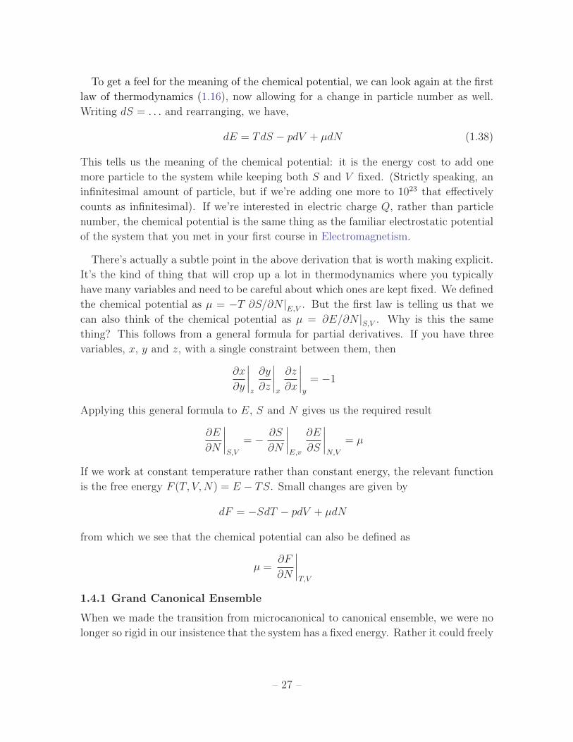
To get a feel for the meaning of the chemical potential, we can look again at the first
law of thermodynamics (1.16), now allowing for a change in particle number as well.
Writing dS = . . . and rearranging, we have,
dE = TdS − pdV + µdN (1.38)
This tells us the meaning of the chemical potential: it is the energy cost to add one
more particle to the system while keeping both S and V fixed. (Strictly speaking, an
infinitesimal amount of particle, but if we’re adding one more to 1023 that effectively
counts as infinitesimal). If we’re interested in electric charge Q, rather than particle
number, the chemical potential is the same thing as the familiar electrostatic potential
of the system that you met in your first course in Electromagnetism.
There’s actually a subtle point in the above derivation that is worth making explicit.
It’s the kind of thing that will crop up a lot in thermodynamics where you typically
have many variables and need to be careful about which ones are kept fixed. We defined
the chemical potential as µ = −T ∂S/∂N |E,V . But the first law is telling us that we
can also think of the chemical potential as µ = ∂E/∂N |S,V . Why is this the same
thing? This follows from a general formula for partial derivatives. If you have three
variables, x, y and z, with a single constraint between them, then
∂x
∂y
∣∣∣∣z
∂y
∂z
∣∣∣∣x
∂z
∂x
∣∣∣∣y
= −1
Applying this general formula to E, S and N gives us the required result
∂E
∂N
∣∣∣∣S,V
= − ∂S
∂N
∣∣∣∣E,v
∂E
∂S
∣∣∣∣N,V
= µ
If we work at constant temperature rather than constant energy, the relevant function
is the free energy F (T, V,N) = E − TS. Small changes are given by
dF = −SdT − pdV + µdN
from which we see that the chemical potential can also be defined as
µ =∂F
∂N
∣∣∣∣T,V
1.4.1 Grand Canonical Ensemble
When we made the transition from microcanonical to canonical ensemble, we were no
longer so rigid in our insistence that the system has a fixed energy. Rather it could freely
– 27 –

exchange energy with the surrounding reservoir, which was kept at a fixed temperature.
We could now imagine the same scenario with any other conserved quantity. For
example, if particles are free to move between the system and the reservoir, then N
is no longer fixed. In such a situation, we will require that the reservoir sits at fixed
chemical potential µ as well as fixed temperature T .
The probability distribution that we need to use in this case is called the grand
canonical ensemble. The probability of finding the system in a state |n〉 depends on both
the energy En and the particle number Nn. (Notice that because N is conserved, the
quantum mechanical operator necessarily commutes with the Hamiltonian so there is
no difficulty in assigning both energy and particle number to each state). We introduce
the grand canonical partition function
Z(T, µ, V ) =∑n
e−β(En−µNn) (1.39)
Re-running the argument that we used for the canonical ensemble, we find the proba-
bility that the system is in state |n〉 to be
p(n) =e−β(En−µNn)
ZIn the canonical ensemble, all the information that we need is contained within the
partition function Z. In the grand canonical ensemble it is contained within Z. The
entropy (1.30) is once again given by
S = kB∂
∂T(T logZ) (1.40)
while differentiating with respect to β gives us
〈E〉 − µ〈N〉 = − ∂
∂βlogZ (1.41)
The average particle number 〈N〉 in the system can then be separately extracted by
〈N〉 =1
β
∂
∂µlogZ (1.42)
and its fluctuations,
∆N2 =1
β2
∂2
∂µ2logZ =
1
β
∂〈N〉∂µ
(1.43)
Just as the average energy is determined by the temperature in the canonical ensemble,
here the average particle number is determined by the chemical potential. The grand
canonical ensemble will simplify several calculations later, especially when we come to
discuss Bose and Fermi gases in Section 3.
– 28 –

The relative size of these fluctuations scales in the same way as the energy fluctua-
tions, ∆N/〈N〉 ∼ 1/√〈N〉, and in the thermodynamic limit N → ∞ results from all
three ensembles coincide. For this reason, we will drop the averaging brackets 〈·〉 from
our notation and simply refer to the average particle number as N .
1.4.2 Grand Canonical Potential
The grand canonical potential Φ is defined by
Φ = F − µN
Φ is a Legendre transform of F , from variable N to µ. This is underlined if we look at
small variations,
dΦ = −SdT − pdV −Ndµ (1.44)
which tells us that Φ should be thought of as a function of temperature, volume and
chemical potential, Φ = Φ(T, V, µ).
We can perform the same algebraic manipulations that gave us F in terms of the
canonical partition function Z, this time using the definitions (1.40) and (1.41)) to
write Φ as
Φ = −kBT logZ (1.45)
1.4.3 Extensive and Intensive Quantities
There is one property of Φ that is rather special and, at first glance, somewhat sur-
prising. This property actually follows from very simple considerations of how different
variables change as we look at bigger and bigger systems.
Suppose we have a system and we double it. That means that we double the volume
V , double the number of particles N and double the energy E. What happens to all our
other variables? We have already seen back in Section 1.2.1 that entropy is additive, so
S also doubles. More generally, if we scale V , N and E by some amount λ, the entropy
must scale as
S(λE, λV, λN) = λS(E, V,N)
Quantities such as E, V , N and S which scale in this manner are called extensive. In
contrast, the variables which arise from differentiating the entropy, such as temperature
1/T = ∂S/∂E and pressure p = T∂S/∂V and chemical potential µ = T∂S/∂N involve
the ratio of two extensive quantities and so do not change as we scale the system: they
are called intensive quantities.
– 29 –

What now happens as we make successive Legendre transforms? The free energy
F = E − TS is also extensive (since E and S are extensive while T is intensive). So it
must scale as
F (T, λV, λN) = λF (T, V,N) (1.46)
Similarly, the grand potential Φ = F − µN is extensive and scales as
Φ(T, λV, µ) = λΦ(T, V, µ) (1.47)
But there’s something special about this last equation, because Φ only depends on a
single extensive variable, namely V . While there are many ways to construct a free
energy F which obeys (1.46) (for example, any function of the form F ∼ V n+1/Nn will
do the job), there is only one way to satisfy (1.47): Φ must be proportional to V . But
we’ve already got a name for this proportionality constant: it is pressure. (Actually, it
is minus the pressure as you can see from (1.44)). So we have the equation
Φ(T, V, µ) = −p(T, µ)V (1.48)
It looks as if we got something for free! If F is a complicated function of V , where
do these complications go after the Legendre transform to Φ? The answer is that the
complications go into the pressure p(T, µ) when expressed as a function of T and µ.
Nonetheless, equation (1.48) will prove to be an extremely economic way to calculate
the pressure of various systems.
1.4.4 Josiah Willard Gibbs (1839-1903)
“Usually, Gibbs’ prose style conveys his meaning in a sufficiently clear way,
using no more than twice as many words as Poincare or Einstein would have
used to say the same thing.”
E.T.Jaynes on the difficulty of reading Gibbs
Gibbs was perhaps the first great American theoretical physicist. Many of the
developments that we met in this chapter are due to him, including the free energy,
the chemical potential and, most importantly, the idea of ensembles. Even the name
“statistical mechanics” was invented by Gibbs.
Gibbs provided the first modern rendering of the subject in a treatise published
shortly before his death. Very few understood it. Lord Rayleigh wrote to Gibbs
suggesting that the book was “too condensed and too difficult for most, I might say
all, readers”. Gibbs disagreed. He wrote back saying the book was only “too long”.
– 30 –

There do not seem to be many exciting stories about Gibbs. He was an undergraduate
at Yale. He did a PhD at Yale. He became a professor at Yale. Apparently he rarely
left New Haven. Strangely, he did not receive a salary for the first ten years of his
professorship. Only when he received an offer from John Hopkins of $3000 dollars a
year did Yale think to pay America’s greatest physicist. They made a counter-offer of
$2000 dollars and Gibbs stayed.
– 31 –

2. Classical Gases
Our goal in this section is to use the techniques of statistical mechanics to describe the
dynamics of the simplest system: a gas. This means a bunch of particles, flying around
in a box. Although much of the last section was formulated in the language of quantum
mechanics, here we will revert back to classical mechanics. Nonetheless, a recurrent
theme will be that the quantum world is never far behind: we’ll see several puzzles,
both theoretical and experimental, which can only truly be resolved by turning on ~.
2.1 The Classical Partition Function
For most of this section we will work in the canonical ensemble. We start by reformu-
lating the idea of a partition function in classical mechanics. We’ll consider a simple
system – a single particle of mass m moving in three dimensions in a potential V (~q).
The classical Hamiltonian of the system3 is the sum of kinetic and potential energy,
H =~p2
2m+ V (~q)
We earlier defined the partition function (1.21) to be the sum over all quantum states
of the system. Here we want to do something similar. In classical mechanics, the state
of a system is determined by a point in phase space. We must specify both the position
and momentum of each of the particles — only then do we have enough information
to figure out what the system will do for all times in the future. This motivates the
definition of the partition function for a single classical particle as the integration over
phase space,
Z1 =1
h3
∫d3qd3p e−βH(p,q) (2.1)
The only slightly odd thing is the factor of 1/h3 that sits out front. It is a quantity
that needs to be there simply on dimensional grounds: Z should be dimensionless so h
must have dimension (length×momentum) or, equivalently, Joules-seconds (Js). The
actual value of h won’t matter for any physical observable, like heat capacity, because
we always take logZ and then differentiate. Despite this, there is actually a correct
value for h: it is Planck’s constant, h = 2π~ ≈ 6.6× 10⁻³⁴ Js.
It is very strange to see Planck’s constant in a formula that is supposed to be classical.
What’s it doing there? In fact, it is a vestigial object, like the male nipple. It is
redundant, serving only as a reminder of where we came from. And the classical world
came from the quantum.3If you haven’t taken the Classical Dynamics course, you should think of the Hamiltonian as the
energy of the system expressed in terms of the position and momentum of the particle.
– 32 –

2.1.1 From Quantum to Classical
It is possible to derive the classical partition function (2.1) directly from the quantum
partition function (1.21) without resorting to hand-waving. It will also show us why
the factor of 1/h sits outside the partition function. The derivation is a little tedious,
but worth seeing. (Similar techniques are useful in later courses when you first meet
the path integral). To make life easier, let’s consider a single particle moving in one
spatial dimension. It has position operator q, momentum operator p and Hamiltonian,
H =p2
2m+ V (q)
If |n〉 is the energy eigenstate with energy En, the quantum partition function is
Z1 =∑n
e−βEn =∑n
〈n|e−βH |n〉 (2.2)
In what follows, we’ll make liberal use of the fact that we can insert the identity operator
anywhere in this expression. Identity operators can be constructed by summing over
any complete basis of states. We’ll need two such constructions, using the position
eigenvectors |q〉 and the momentum eigenvectors |p〉,
1 =
∫dq |q〉〈q| , 1 =
∫dp |p〉〈p|
We start by inserting two copies of the identity built from position eigenstates,
Z1 =∑n
〈n|∫dq |q〉〈q|e−βH
∫dq′|q′〉〈q′|n〉
=
∫dqdq′ 〈q|e−βH |q′〉
∑n
〈q′|n〉〈n|q〉
But now we can replace∑
n |n〉〈n| with the identity matrix and use the fact that
〈q′|q〉 = δ(q′ − q), to get
Z1 =
∫dq 〈q|e−βH |q〉 (2.3)
We see that the result is to replace the sum over energy eigenstates in (2.2) with a
sum (or integral) over position eigenstates in (2.3). If you wanted, you could play the
same game and get the sum over any complete basis of eigenstates of your choosing.
As an aside, this means that we can write the partition function in a basis independent
fashion as
Z1 = Tr e−βH
– 33 –

So far, our manipulations could have been done for any quantum system. Now we want
to use the fact that we are taking the classical limit. This comes about when we try
to factorize e−βH into a momentum term and a position term. The trouble is that this
isn’t always possible when there are matrices (or operators) in the exponent. Recall
that,
eAeB = eA+B+12
[A,B]+...
For us [q, p] = i~. This means that if we’re willing to neglect terms of order ~ — which
is the meaning of taking the classical limit — then we can write
e−βH = e−βp2/2m e−βV (q) +O(~)
We can now start to replace some of the operators in the exponent, like V (q), with
functions V (q). (The notational difference is subtle, but important, in the expressions
below!),
Z1 =
∫dq 〈q|e−βp2/2me−βV (q)|q〉
=
∫dq e−βV (q)〈q|e−βp2/2m|q〉
=
∫dqdpdp′e−βV (q)〈q|p〉〈p|e−βp2/2m|p′〉〈p′|q〉
=1
2π~
∫dqdp e−βH(p,q)
where, in the final line, we’ve used the identity
〈q|p〉 =1√2π~
eipq/~
This completes the derivation.
2.2 Ideal Gas
The first classical gas that we’ll consider consists of N particles trapped inside a box of
volume V . The gas is “ideal”. This simply means that the particles do not interact with
each other. For now, we’ll also assume that the particles have no internal structure,
so no rotational or vibrational degrees of freedom. This situation is usually referred to
as the monatomic ideal gas. The Hamiltonian for each particle is simply the kinetic
energy,
H =~p 2
2m
– 34 –

And the partition function for a single particle is
Z1(V, T ) =1
(2π~)3
∫d3qd3p e−β~p
2/2m (2.4)
The integral over position is now trivial and gives∫d3q = V , the volume of the box.
The integral over momentum is also straightforward since it factorizes into separate
integrals over px, py and pz, each of which is a Gaussian of the form,∫dx e−ax
2
=
√π
a
So we have
Z1 = V
(mkBT
2π~2
)3/2
We’ll meet the combination of factors in the brackets a lot in what follows, so it is
useful to give it a name. We’ll write
Z1 =V
λ3(2.5)
The quantity λ goes by the name of the thermal de Broglie wavelength,
λ =
√2π~2
mkBT(2.6)
λ has the dimensions of length. We will see later that you can think of λ as something
like the average de Broglie wavelength of a particle at temperature T . Notice that it
is a quantum object – it has an ~ sitting in it – so we expect that it will drop out of
any genuinely classical quantity that we compute. The partition function itself (2.5) is
counting the number of these thermal wavelengths that we can fit into volume V .
Z1 is the partition function for a single particle. We have N , non-interacting, particles
in the box so the partition function of the whole system is
Z(N, V, T ) = ZN1 =
V N
λ3N(2.7)
(Full disclosure: there’s a slightly subtle point that we’re brushing under the carpet
here and this equation isn’t quite right. This won’t affect our immediate discussion
and we’ll explain the issue in more detail in Section 2.2.3.)
– 35 –

Figure 8: Deviations from ideal gas law
at sensible densities
Figure 9: Deviations from ideal gas law
at extreme densities
Armed with the partition function Z, we can happily calculate anything that we like.
Let’s start with the pressure, which can be extracted from the partition function by
first computing the free energy (1.36) and then using (1.35). We have
p = −∂F∂V
=∂
∂V(kBT logZ)
=NkBT
V(2.8)
This equation is an old friend – it is the ideal gas law, pV = NkBT , that we all met
in kindergarten. Notice that the thermal wavelength λ has indeed disappeared from
the discussion as expected. Equations of this form, which link pressure, volume and
temperature, are called equations of state. We will meet many throughout this course.
As the plots above show4, the ideal gas law is an extremely good description of gases
at low densities. Gases deviate from this ideal behaviour as the densities increase and
the interactions between atoms becomes important. We will see how this comes about
from the viewpoint of microscopic forces in Section 2.5.
It is worth pointing out that this derivation should calm any lingering fears that
you had about the definition of temperature given in (1.7). The object that we call
T really does coincide with the familiar notion of temperature applied to gases. But
the key property of the temperature is that if two systems are in equilibrium then they
have the same T . That’s enough to ensure that equation (1.7) is the right definition of
temperature for all systems because we can always put any system in equilibrium with
an ideal gas.4Both figures are taken from the web textbook “General Chemistry” and credited to John Hutchin-
son.
– 36 –

2.2.1 Equipartition of Energy
The partition function (2.7) has more in store for us. We can compute the average
energy of the ideal gas,
E = − ∂
∂βlogZ =
3
2NkBT (2.9)
There’s an important, general lesson lurking in this formula. To highlight this, it is
worth repeating our analysis for an ideal gas in arbitrary number of spatial dimensions,
D. A simple generalization of the calculations above shows that
Z =V N
λDN⇒ E =
D
2NkBT
Each particle has D degrees of freedom (because it can move in one of D spatial
directions). And each particle contributes 12DkBT towards the average energy. This
is a general rule of thumb, which holds for all classical systems: the average energy of
each free degree of freedom in a system at temperature T is 12kBT . This is called the
equipartition of energy. As stated, it holds only for degrees of freedom in the absence
of a potential. (There is a modified version if you include a potential). Moreover, it
holds only for classical systems or quantum systems at suitably high temperatures.
We can use the result above to see why the thermal de Broglie wavelength (2.6)
can be thought of as roughly equal to the average de Broglie wavelength of a particle.
Equating the average energy (2.9) to the kinetic energy E = p2/2m tells us that the
average (root mean square) momentum carried by each particle is p ∼√mkBT . In
quantum mechanics, the de Broglie wavelength of a particle is λdB = h/p, which (up
to numerical factors of 2 and π) agrees with our formula (2.6).
Finally, returning to the reality of d = 3 dimensions, we can compute the heat
capacity for a monatomic ideal gas. It is
CV =∂E
∂T
∣∣∣∣V
=3
2NkB (2.10)
2.2.2 The Sociological Meaning of Boltzmann’s Constant
We introduced Boltzmann’s constant kB in our original the definition of entropy (1.2).
It has the value,
kB = 1.381× 10⁻²³ JK−1
In some sense, there is no deep physical meaning to Boltzmann’s constant. It is merely
a conversion factor that allows us to go between temperature and energy, as reflected
– 37 –

in (1.7). It is necessary to include it in the equations only for historical reasons: our
ancestors didn’t realise that temperature and energy were closely related and measured
them in different units.
Nonetheless, we could ask why does kB have the value above? It doesn’t seem a par-
ticularly natural number. The reason is that both the units of temperature (Kelvin)
and energy (Joule) are picked to reflect the conditions of human life. In the everyday
world around us, measurements of temperature and energy involve fairly ordinary num-
bers: room temperature is roughly 300K; the energy required to lift an apple back up
to the top of the tree is a few Joules. Similarly, in an everyday setting, all the measur-
able quantities — p, V and T — in the ideal gas equation are fairly normal numbers
when measured in SI units. The only way this can be true is if the combination NkBis a fairly ordinary number, of order one. In other words the number of atoms must be
huge,
N ∼ 1023 (2.11)
This then is the real meaning of the value of Boltzmann’s constant: atoms are small.
It’s worth stressing this point. Atoms aren’t just small: they’re really really small.
1023 is an astonishingly large number. The number of grains of sand in all the beaches
in the world is around 1018. The number of stars in our galaxy is about 1011. The
number of stars in the entire visible Universe is probably around 1022. And yet the
number of water molecules in a cup of tea is more than 1023.
Chemist Notation
While we’re talking about the size of atoms, it is probably worth reminding you of the
notation used by chemists. They too want to work with numbers of order one. For
this reason, they define a mole to be the number of atoms in one gram of Hydrogen.
(Actually, it is the number of atoms in 12 grams of Carbon-12, but this is roughly the
same thing). The mass of Hydrogen is 1.6 × 10⁻²⁷ Kg, so the number of atoms in a
mole is Avogadro’s number,
NA ≈ 6× 10²³
The number of moles in our gas is then n = N/NA and the ideal gas law can be written
as
pV = nRT
where R = NAkB is the called the Universal gas constant. Its value is a nice sensible
number with no silly power in the exponent: R ≈ 8 JK−1mol−1.
– 38 –
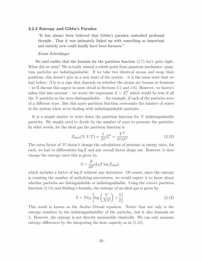
2.2.3 Entropy and Gibbs’s Paradox
“It has always been believed that Gibbs’s paradox embodied profound
thought. That it was intimately linked up with something so important
and entirely new could hardly have been foreseen.”
Erwin Schrodinger
We said earlier that the formula for the partition function (2.7) isn’t quite right.
What did we miss? We actually missed a subtle point from quantum mechanics: quan-
tum particles are indistinguishable. If we take two identical atoms and swap their
positions, this doesn’t give us a new state of the system – it is the same state that we
had before. (Up to a sign that depends on whether the atoms are bosons or fermions
– we’ll discuss this aspect in more detail in Sections 3.5 and 3.6). However, we haven’t
taken this into account – we wrote the expression Z = ZN1 which would be true if all
the N particles in the were distinguishable — for example, if each of the particles were
of a different type. But this naive partition function overcounts the number of states
in the system when we’re dealing with indistinguishable particles.
It is a simple matter to write down the partition function for N indistinguishable
particles. We simply need to divide by the number of ways to permute the particles.
In other words, for the ideal gas the partition function is
Zideal(N, V, T ) =1
N !ZN
1 =V N
N !λ3N(2.12)
The extra factor of N ! doesn’t change the calculations of pressure or energy since, for
each, we had to differentiate logZ and any overall factor drops out. However, it does
change the entropy since this is given by,
S =∂
∂T(kBT logZideal)
which includes a factor of logZ without any derivative. Of course, since the entropy
is counting the number of underlying microstates, we would expect it to know about
whether particles are distinguishable or indistinguishable. Using the correct partition
function (2.12) and Stirling’s formula, the entropy of an ideal gas is given by,
S = NkB
[log
(V
Nλ3
)+
5
2
](2.13)
This result is known as the Sackur-Tetrode equation. Notice that not only is the
entropy sensitive to the indistinguishability of the particles, but it also depends on
λ. However, the entropy is not directly measurable classically. We can only measure
entropy differences by the integrating the heat capacity as in (1.10).
– 39 –

The benefit of adding an extra factor of N ! was noticed before the advent of quantum
mechanics by Gibbs. He was motivated by the change in entropy of mixing between
two gases. Suppose that we have two different gases, say red and blue. Each has the
same number of particles N and sits in a volume V, separated by a partition. When the
partition is removed the gases mix and we expect the entropy to increase. But if the
gases are of the same type, removing the partition shouldn’t change the macroscopic
state of the gas. So why should the entropy increase? This is referred to as the Gibb’s
paradox. Including the factor of N ! in the partition function ensures that the entropy
does not increase when identical atoms are mixed5
2.2.4 The Ideal Gas in the Grand Canonical Ensemble
It is worth briefly looking at the ideal gas in the grand canonical ensemble. Recall
that in such an ensemble, the gas is free to exchange both energy and particles with
the outside reservoir. You could think of the system as some fixed subvolume inside
a much larger gas. If there are no walls to define this subvolume then particles, and
hence energy, can happily move in and out. We can ask how many particles will, on
average, be inside this volume and what fluctuations in particle number will occur.
More importantly, we can also start to gain some intuition for this strange quantity
called the chemical potential, µ.
The grand partition function (1.39) for the ideal gas is
Zideal(µ, V, T ) =∞∑N=0
eβµNZideal(N, V, T ) = exp
(eβµV
λ3
)From this we can determine the average particle number,
N =1
β
∂
∂µlogZ =
eβµV
λ3
Which, rearranging, gives
µ = kBT log
(λ3N
V
)(2.14)
If λ3 < V/N then the chemical potential is negative. Recall that λ is roughly the
average de Broglie wavelength of each particle, while V/N is the average volume taken
5Be warned however: a closer look shows that the Gibbs paradox is rather toothless and, in the
classical world, there is no real necessity to add the N !. A clear discussion of these issues can be found
in E.T. Jaynes’ article “The Gibbs Paradox” which you can download from the course website.
– 40 –

up by each particle. But whenever the de Broglie wavelength of particles becomes
comparable to the inter-particle separation, then quantum effects become important. In
other words, to trust our classical calculation of the ideal gas, we must have λ3 V/N
and, correspondingly, µ < 0.
At first sight, it is slightly strange that µ is negative. When we introduced µ in
Section 1.4.1, we said that it should be thought of as the energy cost of adding an extra
particle to the system. Surely that energy should be positive! To see why this isn’t the
case, we should look more closely at the definition. From the energy variation (1.38),
we have
µ =∂E
∂N
∣∣∣∣S,V
So the chemical potential should be thought of as the energy cost of adding an extra
particle at fixed entropy and volume. But adding a particle will give more ways to share
the energy around and so increase the entropy. If we insist on keeping the entropy fixed,
then we will need to reduce the energy when we add an extra particle. This is why we
have µ < 0 for the classical ideal gas.
There are situations where µ > 0. This can occur if we have a suitably strong
repulsive interaction between particles so that there’s a large energy cost associated to
throwing in one extra. We also have µ > 0 for fermion systems at low temperatures as
we will see in Section 3.6.
We can also compute the fluctuation in the particle number,
∆N2 =1
β2
∂2
∂µ2logZideal = N
As promised in Section 1.4.1, the relative fluctuations ∆N/〈N〉 = 1/√N are vanishingly
small in the thermodynamic N →∞ limit.
Finally, it is very easy to compute the equation of state in the grand canonical
ensemble because (1.45) and (1.48) tell us that
pV = kBT logZ = kBTeβµV
λ3= kBTN (2.15)
which gives us back the ideal gas law.
– 41 –

Figure 10: Maxwell distribution for Noble gases: He, Ne, Ar and Xe.
2.3 Maxwell Distribution
Our discussion above focusses on understanding macroscopic properties of the gas such
as pressure or heat capacity. But we can also use the methods of statistical mechanics
to get a better handle on the microscopic properties of the gas. Like everything else,
the information is hidden in the partition function. Let’s return to the form of the
single particle partition function (2.4) before we do the integrals. We’ll still do the
trivial spatial integral∫d3q = V , but we’ll hold off on the momentum integral and
instead change variables from momentum to velocity, ~p = m~v. Then the single particle
partition function is
Z1 =m3V
(2π~)3
∫d3v e−βm~v
2/2 =4πm3V
(2π~)3
∫dv v2e−βmv
2/2
We can compare this to the original definition of the partition function: the sum over
states of the probability of that state. But here too, the partition function is written as
a sum, now over speeds. The integrand must therefore have the interpretation as the
probability distribution over speeds. The probability that the atom has speed between
v and v + dv is
f(v)dv = N v2e−mv2/2kBT dv (2.16)
where the normalization factor N can be determined by insisting that probabilities
sum to one,∫∞
0f(v) dv = 1, which gives
N = 4π
(m
2πkBT
)3/2
– 42 –

This is the Maxwell distribution. It is sometimes called the Maxwell-Boltzmann distri-
bution. Figure 10 shows this distribution for a variety of gases with different masses
at the same temperature, from the slow heavy Xenon (purple) to light, fast Helium
(blue). We can use it to determine various average properties of the speeds of atoms
in a gas. For example, the mean square speed is
〈v2〉 =
∫ ∞0
dv v2f(v) =3kBT
m
This is in agreement with the equipartition of energy: the average kinetic energy of the
gas is E = 12m〈v2〉 = 3
2kBT .
Maxwell’s Argument
The above derivation tells us the distribution of velocities in a non-interacting gas of
particles. Remarkably, the Maxwell distribution also holds in the presence of any in-
teractions. In fact, Maxwell’s original derivation of the distribution makes no reference
to any properties of the gas. It is very slick!
Let’s first think about the distribution of velocities in the x direction; we’ll call this
distribution φ(vx). Rotational symmetry means that we must have the same distri-
bution of velocities in both the y and z directions. However, rotational invariance
also requires that the full distribution can’t depend on the direction of the velocity; it
can only depend on the speed v =√v2x + v2
y + v2z . This means that we need to find
functions F (v) and φ(vx) such that
F (v) dvxdvydvz = φ(vx)φ(vy)φ(vz) dvxdvydvz
It doesn’t look as if we possibly have enough information to solve this equation for
both F and φ. But, remarkably, there is only one solution. The only function which
satisfies this equation is
φ(vx) = Ae−Bv2x
for some constants A and B. Thus the distribution over speeds must be
F (v) dvxdvydvz = 4πv2F (v) dv = 4πA3v2e−Bv2
dv
We see that the functional form of the distribution arises from rotational invariance
alone. To determine the coefficient B = m/2kBT we need the more elaborate tech-
niques of statistical mechanics that we saw above. (In fact, one can derive it just from
equipartition of energy).
– 43 –

2.3.1 A History of Kinetic Theory
The name kinetic theory refers to the understanding the properties of gases through
their underlying atomic constituents. The discussion given above barely scratches the
surface of this important subject.
Kinetic theory traces its origin to the work of Daniel Bernoulli in 1738. He was
the first to argue that the phenomenon that we call pressure is due to the constant
bombardment of tiny atoms. His calculation is straightforward. Consider a cubic box
with sides of length L. Suppose that an atom travelling with momentum vx in the x
direction bounces elastically off a wall so that it returns with velocity −vx. The particle
experiences a change in momentum is ∆px = 2mvx. Since the particle is trapped in a
box, it will next hit the wall at a time ∆t = 2L/vx later. This means that the force on
the wall due to this atom is
F =∆px∆t
=mv2
x
L
Summing over all the atoms which hit the wall, the force is
F =Nm〈v2
x〉L
where 〈v2x〉 is the average velocity in the x-direction. Using the same argument as we
gave in Maxwell’s derivation above, we must have 〈v2x〉 = 〈v2〉/3. Thus F = Nm〈v〉2/3L
and the pressure, which is force per area, is given be
p =Nm〈v2〉
3L3=Nm〈v2〉
3V
If this equation is compared to the ideal gas law (which, at the time, had only experi-
mental basis) one concludes that the phenomenon of temperature must arise from the
kinetic energy of the gas. Or, more precisely, one finds the equipartition result that we
derived previously: 12m〈v2〉 = 3
2kBT .
After Bernoulli’s pioneering work, kinetic theory languished. No one really knew
what to do with his observation nor how to test the underlying atomic hypothesis.
Over the next century, Bernouilli’s result was independently rediscovered by a number
of people, all of whom were ignored by the scientific community. One of the more
interesting attempts was by John Waterson, a Scottish engineer and naval instructor
working for the East India Company in Bombay. Waterson was considered a crackpot.
His 1843 paper was rejected by the Royal Society as “nothing but nonsense” and
he wrote up his results in a self-published book with the wonderfully crackpot title
“Thoughts on Mental Functions”.
– 44 –

The results of Bernouilli and Waterson finally became accepted only after they were
re-rediscovered by more established scientists, most notably Rudolph Clausius who, in
1857, extended these ideas to rotating and vibrating molecules. Soon afterwards, in
1859, Maxwell gave the derivation of the distribution of velocities that we saw above.
This is often cited as the first statistical law of physics. But Maxwell was able to take
things further. He used kinetic theory to derive the first genuinely new prediction of
the atomic hypothesis: that the viscosity of a gas is independent of its density. Maxwell
himself wrote,
”Such a consequence of the mathematical theory is very startling and the
only experiment I have met with on the subject does not seem to confirm
it.”
Maxwell decided to rectify the situation. With help from his wife, he spent several years
constructing an experimental apparatus in his attic which was capable of providing the
first accurate measurements of viscosity of gases6. His surprising theoretical prediction
was confirmed by his own experiment.
There are many further developments in kinetic theory which we will not cover in
this course. Perhaps the most important is the Boltzmann equation. This describes
the evolution of a particle’s probability distribution in position and momentum space
as it collides with other particles. Stationary, unchanging, solutions bring you back to
the Maxwell-Boltzmann distribution, but the equation also provides a framework to go
beyond the equilibrium description of a gas. You can read about this in the lecture
notes on Kinetic Theory.
2.4 Diatomic Gas
“I must now say something about these internal motions, because the great-
est difficulty which the kinetic theory of gases has yet encountered belongs
to this part of the subject”.
James Clerk Maxwell, 1875
Consider a molecule that consists of two atoms in a bound state. We’ll construct
a very simple physicist’s model of this molecule: two masses attached to a spring. As
well as the translational degrees of freedom, there are two further ways in which the
molecule can move
6You can see the original apparatus down the road in the corridor of the Cavendish lab. Or, if you
don’t fancy the walk, you can simply click here:
http://www-outreach.phy.cam.ac.uk/camphy/museum/area1/exhibit1.htm
– 45 –

• Rotation: the molecule can rotate rigidly about the two axes perpendicular to
the axis of symmetry, with moment of inertia I. (For now, we will neglect the
rotation about the axis of symmetry. It has very low moment of inertia which
will ultimately mean that it is unimportant).
• Vibration: the molecule can oscillate along the axis of symmetry
We’ll work under the assumption that the rotation and vibration modes are indepen-
dent. In this case, the partition function for a single molecule factorises into the product
of the translation partition function Ztrans that we have already calculated (2.5) and
the rotational and vibrational contributions,
Z1 = ZtransZrotZvib
We will now deal with Zrot and Zvib in turn.
Rotation
The Lagrangian for the rotational degrees of freedom is7
Lrot =1
2I(θ2 + sin2 θφ2) (2.17)
The conjugate momenta are therefore
pθ =∂Lrot
∂θ= Iθ , pφ =
∂Lrot
∂φ= I sin2 θ φ
from which we get the Hamiltonian for the rotating diatomic molecule,
Hrot = θpθ + φpφ − L =p2θ
2I+
p2φ
2I sin2 θ(2.18)
The rotational contribution to the partition function is then
Zrot =1
(2π~)2
∫dθdφdpθdpφ e
−βHrot
=1
(2π~)2
√2πI
β
∫ π
0
dθ
√2πI sin2 θ
β
∫ 2π
0
dφ
=2IkBT
~2(2.19)
7See, for example, Section 3.6 of the lecture notes on Classical Dynamics
– 46 –

From this we can compute the average rotational energy of each molecule,
Erot = kBT
If we now include the translational contribution (2.5), the partition function for a di-
atomic molecule that can spin and move, but can’t vibrate, is given by Z1 = ZtransZrot ∼(kBT )5/2, and the partition function for a gas of these object Z = ZN
1 /N !, from which
we compute the energy E = 52NkBT and the heat capacity,
CV =5
2kBN
In fact we can derive this result simply from equipartition of energy: there are 3
translational modes and 2 rotational modes, giving a contribution of 5N × 12kBT to the
energy.
Vibrations
The Hamiltonian for the vibrating mode is simply a harmonic oscillator. We’ll denote
the displacement away from the equilibrium position by ζ. The molecule vibrates
with some frequency ω which is determined by the strength of the atomic bond. The
Hamiltonian is then
Hvib =p2ζ
2m+
1
2mω2ζ2
from which we can compute the partition function
Zvib =1
2π~
∫dζdpζe
−βHvib =kBT
~ω(2.20)
The average vibrational energy of each molecule is now
Evib = kBT
(You may have anticipated 12kBT since the harmonic oscillator has just a single degree
of freedom, but equipartition works slightly differently when there is a potential energy.
You will see another example on the problem sheet from which it is simple to deduce
the general form).
Putting together all the ingredients, the contributions from translational motion,
rotation and vibration give the heat capacity
CV =7
2NkB
– 47 –

Figure 11: The heat capacity of Hydrogen gas H2. The graph was created by P. Eyland.
This result depends on neither the moment of inertia, I, nor the stiffness of the molec-
ular bond, ω. A molecule with large I will simply spin more slowly so that the average
rotational kinetic energy is kBT ; a molecule attached by a stiff spring with high ω will
vibrate with smaller amplitude so that the average vibrational energy is kBT . This
ensures that the heat capacity is constant.
Great! So the heat capacity of a diatomic gas is 72NkB. Except it’s not! An idealised
graph of the heat capacity for H2, the simplest diatomic gas, is shown in Figure 11. At
suitably high temperatures, around 5000K, we do see the full heat capacity that we
expect. But at low temperatures, the heat capacity is that of monatomic gas. And, in
the middle, it seems to rotate, but not vibrate. What’s going on? Towards the end of
the nineteenth century, scientists were increasingly bewildered about this behaviour.
What’s missing in the discussion above is something very important: ~. The succes-
sive freezing out of vibrational and rotational modes as the temperature is lowered is
a quantum effect. In fact, this behaviour of the heat capacities of gases was the first
time that quantum mechanics revealed itself in experiment. We’re used to thinking of
quantum mechanics as being relevant on small scales, yet here we see that affects the
physics of gases at temperatures of 2000K. But then, that is the theme of this course:
how the microscopic determines the macroscopic. We will return to the diatomic gas
in Section 3.4 and understand its heat capacity including the relevant quantum effects.
2.5 Interacting Gas
Until now, we’ve only discussed free systems; particles moving around unaware of each
other. Now we’re going to turn on interactions. Here things get much more interesting.
– 48 –

And much more difficult. Many of the most important unsolved problems in physics
are to do with the interactions between large number of particles. Here we’ll be gentle.
We’ll describe a simple approximation scheme that will allow us to begin to understand
the effects of interactions between particles.
We’ll focus once more on the monatomic gas. The ideal gas law is exact in the limit
of no interactions between atoms. This is a good approximation when the density of
atoms N/V is small. Corrections to the ideal gas law are often expressed in terms of a
density expansion, known as the virial expansion. The most general equation of state
is,
p
kBT=N
V+B2(T )
N2
V 2+B3(T )
N3
V 3+ . . . (2.21)
where the functions Bj(T ) are known as virial coefficients.
Our goal is to compute the virial coefficients from first principles, starting from a
knowledge of the underlying potential energy U(r) between two neutral atoms separated
by a distance r. This potential has two important features:
• An attractive 1/r6 force. This arises from fluctuating dipoles of the neutral atoms.
Recall that two permanent dipole moments, p1 and p2, have a potential energy
which scales as p1p2/r3. Neutral atoms don’t have permanent dipoles, but they
can acquire a temporary dipole due to quantum fluctuations. Suppose that the
first atom has an instantaneous dipole p1. This will induce an electric field which
is proportional to E ∼ p1/r3 which, in turn, will induce a dipole of the second
atom p2 ∼ E ∼ p1/r3. The resulting potential energy between the atoms scales
as p1p2/r3 ∼ 1/r6. This is sometimes called the van der Waals interaction.
• A rapidly rising repulsive interaction at short distances, arising from the Pauli
exclusion principle that prevents two atoms from occupying the same space. For
our purposes, the exact form of this repulsion is not so relevant: just as long as
it’s big. (The Pauli exclusion principle is a quantum effect. If the exact form
of the potential is important then we really need to be dealing with quantum
mechanics all along. We will do this in the next section).
One very common potential that is often used to model the force between atoms is the
Lennard-Jones potential,
U(r) ∼(r0
r
)12
−(r0
r
)6
(2.22)
The exponent 12 is chosen only for convenience: it simplifies certain calculations be-
cause 12 = 2× 6.
– 49 –

An even simpler form of the potential incorporates a hard core repulsion, in which
the particles are simply forbidden from closer than a U(r)
rr0
Figure 12:
fixed distance by imposing an infinite potential,
U(r) =
∞ r < r0
−U0
(r0r
)6r ≥ r0
(2.23)
The hard-core potential with van der Waals attraction
is sketched to the right. We will see shortly that the
virial coefficients are determined by increasingly dif-
ficult integrals involving the potential U(r). For this
reason, it’s best to work with a potential that’s as
simple as possible. When we come to do some actual
calculations we will use the form (2.23).
2.5.1 The Mayer f Function and the Second Virial Coefficient
We’re going to change notation and call the positions of the particles ~r instead of ~q.
(The latter notation was useful to stress the connection to quantum mechanics at the
beginning of this Section, but we’ve now left that behind!). The Hamiltonian of the
gas is
H =N∑i=1
p2i
2m+∑i>j
U(rij)
where rij = |~ri − ~rj| is the separation between particles. The restriction i > j on the
final sum ensures that we sum over each pair of particles exactly once. The partition
function is then
Z(N, V, T ) =1
N !
1
(2π~)3N
∫ N∏i=1
d3pid3ri e
−βH
=1
N !
1
(2π~)3N
[∫ ∏i
d3pi e−β
∑j p
2j/2m
]×
[∫ ∏i
d3ri e−β
∑j<k U(rjk)
]=
1
N !λ3N
∫ ∏i
d3ri e−β
∑j<k U(rjk)
where λ is the thermal wavelength that we met in (2.6). We still need to do the integral
over positions. And that looks hard! The interactions mean that the integrals don’t
– 50 –

factor in any obvious way. What to do? One obvious way thing to try is to Taylor
expand (which is closely related to the so-called cumulant expansion in this context)
e−β∑
j<k U(rjk) = 1− β∑j<k
U(rjk) +β2
2
∑j<k,l<m
U(rjk)U(rlm) + . . .
Unfortunately, this isn’t so useful. We want each term to be smaller than the preceding
one. But as rij → 0, the potential U(rij) → ∞, which doesn’t look promising for an
expansion parameter.
Instead of proceeding with the naive Taylor expansion, we will instead choose to
work with the following quantity, usually called the Mayer f function,
f(r) = e−βU(r) − 1 (2.24)
This is a nicer expansion parameter. When the particles are far separated at r → ∞,
f(r) → 0. However, as the particles come close and r → 0, the Mayer function
approaches f(r) → −1. We’ll proceed by trying to construct a suitable expansion in
terms of f . We define
fij = f(rij)
Then we can write the partition function as
Z(N, V, T ) =1
N !λ3N
∫ ∏i
d3ri∏j>k
(1 + fjk)
=1
N !λ3N
∫ ∏i
d3ri
(1 +
∑j>k
fjk +∑
j>k,l>m
fjkflm + . . .
)(2.25)
The first term simply gives a factor of the volume V for each integral, so we get V N .
The second term has a sum, each element of which is the same. They all look like∫ N∏i=1
d3ri f12 = V N−2
∫d3r1d
3r2 f(r12) = V N−1
∫d3r f(r)
where, in the last equality, we’ve simply changed integration variables from ~r1 and ~r2
to the centre of mass ~R = 12(~r1 + ~r2) and the separation ~r = ~r1 − ~r2. (You might
worry that the limits of integration change in the integral over ~r, but the integral over
f(r) only picks up contributions from atomic size distances and this is only actually a
problem close to the boundaries of the system where it is negligible). There is a term
– 51 –

like this for each pair of particles – that is 12N(N − 1) such terms. For N ∼ 1023, we
can just call this a round 12N2. Then, ignoring terms quadratic in f and higher, the
partition function is approximately
Z(N, V, T ) =V N
N !λ3N
(1 +
N2
2V
∫d3r f(r) + . . .
)= Zideal
(1 +
N
2V
∫d3r f(r) + . . .
)Nwhere we’ve used our previous result that Zideal = V N/N !λ3N . We’ve also engaged in
something of a sleight of hand in this last line, promoting one power of N from in front
of the integral to an overall exponent. Massaging the expression in this way ensures
that the free energy is proportional to the number of particles as one would expect:
F = −kBT logZ = Fideal −NkBT log
(1 +
N
2V
∫d3r f(r)
)(2.26)
However, if you’re uncomfortable with this little trick, it’s not hard to convince yourself
that the result (2.27) below for the equation of state doesn’t depend on it. We will also
look at the expansion more closely in the following section and see how all the higher
order terms work out.
From the expression (2.26) for the free energy, it is clear that we are indeed performing
an expansion in density of the gas since the correction term is proportional to N/V .
This form of the free energy will give us the second virial coefficient B2(T ).
We can be somewhat more precise about what it means to be at low density. The
exact form of the integral∫d3rf(r) depends on the potential, but for both the Lennard-
Jones potential (2.22) and the hard-core repulsion (2.23), the integral is approximately∫d3rf(r) ∼ r3
0, where r0 is roughly the minimum of the potential. (We’ll compute the
integral exactly below for the hard-core potential). For the expansion to be valid, we
want each term with an extra power of f to be smaller than the preceding one. (This
statement is actually only approximately true. We’ll be more precise below when we
develop the cluster expansion). That means that the second term in the argument of
the log should be smaller than 1. In other words,
N
V 1
r30
The left-hand side is the density of the gas. The right-hand side is atomic density. Or,
equivalently, the density of a substance in which the atoms are packed closely together.
But we have a name for such substances – we call them liquids! Our expansion is valid
for densities of the gas that are much lower than that of the liquid state.
– 52 –

2.5.2 van der Waals Equation of State
We can use the free energy (2.26) to compute the pressure of the gas. Expanding the
logarithm as log(1 + x) ≈ x we get
p = −∂F∂V
=NkBT
V
(1− N
2V
∫d3rf(r) + . . .
)As expected, the pressure deviates from that of an ideal gas. We can characterize this
by writing
pV
NkBT= 1− N
2V
∫d3r f(r) (2.27)
To understand what this is telling us, we need to compute∫d3rf(r). Firstly let’s look
at two trivial examples:
Repulsion: Suppose that U(r) > 0 for all separations r with U(r = ∞) = 0. Then
f = e−βU − 1 < 0 and the pressure increases, as we’d expect for a repulsive interaction.
Attraction: If U(r) < 0, we have f > 0 and the pressure decreases, as we’d expect
for an attractive interaction.
What about a more realistic interaction that is attractive at long distances and
repulsive at short? We will compute the equation of state of a gas using the hard-core
potential with van der Waals attraction (2.23). The integral of the Mayer f function is∫d3r f(r) =
∫ r0
0
d3r(−1) +
∫ ∞r0
d3r (e+βU0(r0/r)6 − 1) (2.28)
We’ll approximate the second integral in the high temperature limit, βU0 1, where
e+βU0(r0/r)6 ≈ 1 + βU0(r0/r)6. Then∫
d3r f(r) = −4π
∫ r0
0
dr r2 +4πU0
kBT
∫ ∞r0
drr6
0
r4(2.29)
=4πr3
0
3
(U0
kBT− 1
)Inserting this into (2.27) gives us an expression for the equation of state,
pV
NkBT= 1− N
V
(a
kBT− b)
– 53 –

We recognise this expansion as capturing the second virial coefficient in (2.21) as
promised. The constants a and b are defined by
a =2πr3
0U0
3, b =
2πr30
3
It is actually slightly more useful to write this in the form kBT = . . .. We can multiply
through by kBT then, rearranging we have
kBT =V
N
(p+
N2
V 2a
)(1 +
N
Vb
)−1
Since we’re working in an expansion in density, N/V , we’re at liberty to Taylor expand
the last bracket, keeping only the first two terms. We get
kBT =
(p+
N2
V 2a
)(V
N− b)
(2.30)
This is the famous van der Waals equation of state for a gas. We stress again the limita-
tions of our analysis: it is valid only at low densities and (because of our approximation
when performing the integral (2.28)) at high temperatures.
We will return to the van der Waals equation in Section 5 where we’ll explore many
of its interesting features. For now, we can get a feeling for the physics behind this
equation of state by rewriting it in yet another way,
p =NkBT
V − bN− aN
2
V 2(2.31)
The constant a contains a factor of U0 and so capures the effectr
0
r0/2
Figure 13:
of the attractive interaction at large distances. We see that
its role is to reduce the pressure of the gas. The reduction in
pressure is proportional to the density squared because this is,
in turn, proportional to the number of pairs of particles which
feel the attractive force. In contrast, b only contains r0 and
arises due to the hard-core repulsion in the potential. Its effect
is the reduce the effective volume of the gas because of the space
taken up by the particles.
It is worth pointing out where some quizzical factors of two come from in b = 2πr30/3.
Recall that r0 is the minimum distance that two atoms can approach. If we think of the
each atom as a hard sphere, then they have radius r0/2 and volume 4π(r0/2)3/3. Which
isn’t equal to b. However, as illustrated in the figure, the excluded volume around each
– 54 –

atom is actually Ω = 4πr30/3 = 2b. So why don’t we have Ω sitting in the denominator
of the van der Waals equation rather than b = Ω/2? Think about adding the atoms
one at a time. The first guy can move in volume V ; the second in volume V − Ω; the
third in volume V − 2Ω and so on. For Ω V , the total configuration space available
to the atoms is
1
N !
N∏m=1
(V −mΩ) ≈ V N
N !
(1− N2
2
Ω
V+ . . .
)≈ 1
N !
(V − NΩ
2
)NAnd there’s that tricky factor of 1/2.
Above we computed the equation of state for the dipole van der Waals interaction
with hard core potential. But our expression (2.27) can seemingly be used to compute
the equation of state for any potential between atoms. However, there are limitations.
Looking back to the integral (2.29), we see that a long-range force of the form 1/rn
will only give rise to a convergent integral for n ≥ 4. This means that the techniques
described above do not work for long-range potentials with fall-off 1/r3 or slower. This
includes the important case of 1/r Coulomb interactions.
2.5.3 The Cluster Expansion
Above we computed the leading order correction to the ideal gas law. In terms of the
virial expansion (2.21) this corresponds to the second virial coefficient B2. We will now
develop the full expansion and explain how to compute the higher virial coefficients.
Let’s go back to equation (2.25) where we first expressed the partition function in
terms of f ,
Z(N, V, T ) =1
N !λ3N
∫ ∏i
d3ri∏j>k
(1 + fjk)
=1
N !λ3N
∫ ∏i
d3ri
(1 +
∑j>k
fjk +∑
j>k,l>m
fjkflm + . . .
)(2.32)
Above we effectively related the second virial coefficient to the term linear in f : this is
the essence of the equation of state (2.27). One might think that terms quadratic in f
give rise to the third virial coefficient and so on. But, as we’ll now see, the expansion
is somewhat more subtle than that.
– 55 –
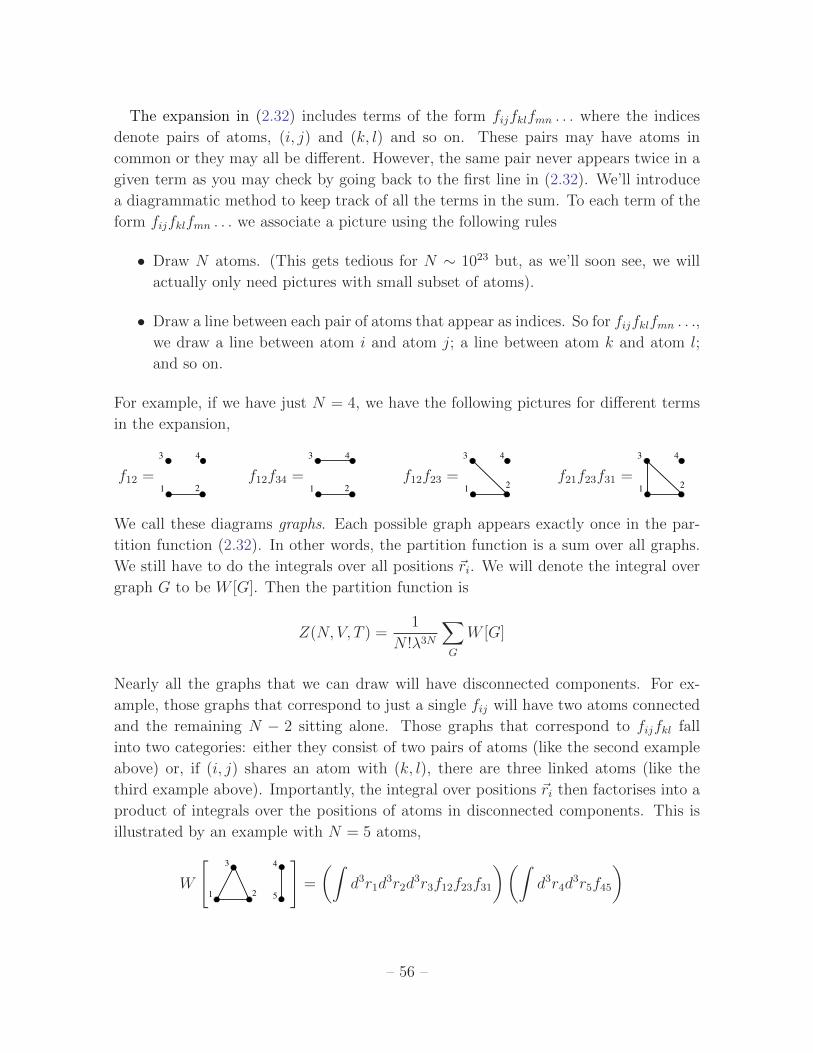
The expansion in (2.32) includes terms of the form fijfklfmn . . . where the indices
denote pairs of atoms, (i, j) and (k, l) and so on. These pairs may have atoms in
common or they may all be different. However, the same pair never appears twice in a
given term as you may check by going back to the first line in (2.32). We’ll introduce
a diagrammatic method to keep track of all the terms in the sum. To each term of the
form fijfklfmn . . . we associate a picture using the following rules
• Draw N atoms. (This gets tedious for N ∼ 1023 but, as we’ll soon see, we will
actually only need pictures with small subset of atoms).
• Draw a line between each pair of atoms that appear as indices. So for fijfklfmn . . .,
we draw a line between atom i and atom j; a line between atom k and atom l;
and so on.
For example, if we have just N = 4, we have the following pictures for different terms
in the expansion,
f12 =1 2
3 4
f12f34 =1 2
3 4
f12f23 =1
3 4
2f21f23f31 =
1
3 4
2
We call these diagrams graphs. Each possible graph appears exactly once in the par-
tition function (2.32). In other words, the partition function is a sum over all graphs.
We still have to do the integrals over all positions ~ri. We will denote the integral over
graph G to be W [G]. Then the partition function is
Z(N, V, T ) =1
N !λ3N
∑G
W [G]
Nearly all the graphs that we can draw will have disconnected components. For ex-
ample, those graphs that correspond to just a single fij will have two atoms connected
and the remaining N − 2 sitting alone. Those graphs that correspond to fijfkl fall
into two categories: either they consist of two pairs of atoms (like the second example
above) or, if (i, j) shares an atom with (k, l), there are three linked atoms (like the
third example above). Importantly, the integral over positions ~ri then factorises into a
product of integrals over the positions of atoms in disconnected components. This is
illustrated by an example with N = 5 atoms,
W
[1
3 4
52
]=
(∫d3r1d
3r2d3r3f12f23f31
)(∫d3r4d
3r5f45
)
– 56 –

We call the disconnected components of the graph clusters. If a cluster has l atoms, we
will call it an l-cluster. The N = 5 example above has a single 3-cluster and a single
2-cluster. In general, a graph G will split into ml l-clusters. Clearly, we must have
N∑l=1
mll = N (2.33)
Of course, for a graph with only a few lines and lots of atoms, nearly all the atoms will
be in lonely 1-clusters.
We can now make good on the promise above that we won’t have to draw all N ∼ 1023
atoms. The key idea is that we can focus on clusters of l-atoms. We will organise the
expansion in such a way that the (l+ 1)-clusters are less important than the l-clusters.
To see how this works, let’s focus on 3-clusters for now. There are four different ways
that we can have a 3-cluster,
1
3
2 1
3
2 1
3
2 1
3
2
Each of these 3-clusters will appear in a graph with any other combination of clusters
among the remaining N−3 atoms. But since clusters factorise in the partition function,
we know that Z must include a factor
U3 ≡∫d3r1d
3r2d3r3
(1
3
2 1
3
2 1
3
2 1
3
2
+ + +
)U3 contains terms of order f 2 and f 3. It turns out that this is the correct way to arrange
the expansion: not in terms of the number of lines in the diagram, which is equal to
the power of f , but instead in terms of the number of atoms that they connect. The
partition function will similarly contain factors associated to all other l-clusters. We
define the corresponding integrals as
Ul ≡∫ l∏
i=1
d3ri∑
G∈l-cluster
G (2.34)
Notice that U1 is simply the integral over space, namely U1 = V . The full partition
function must be a product of Ul’s. The tricky part is to get all the combinatoric factors
right to make sure that you count each graph exactly once. The sum over graphs G
that appears in the partition function turns out to be∑G
W [G] = N !∑ml
∏l
Umll
(l!)mlml!(2.35)
– 57 –

The product N !/∏
l ml!(l!)ml counts the number of ways to split the particles into ml
l-clusters, while ignoring the different ways to internally connect each cluster. This is
the right thing to do since the different internal connections are taken into account in
the integral Ul.
Combinatoric arguments are not always transparent. Let’s do a couple of checks to
make sure that this is indeed the right answer. Firstly, consider N = 4 atoms split into
two 2-clusters (i.e m2 = 2). There are three such diagrams, f12f34 = , f13f24 = ,
and f14f23 = . Each of these gives the same answer when integrated, namely U22 so
the final result should be 3U22 . We can check this against the relevant terms in (2.35)
which are 4!U22/2!22! = 3U2
2 as expected.
Another check: N = 5 atoms with m2 = m3 = 1. All diagrams come in the
combinations
U3U2 =
∫ 5∏i=1
d3ri
(++ +
)together with graphs that are related by permutations. The permutations are fully
determined by the choice of the two atoms that sit in the pair: there are 10 such choices.
The answer should therefore be 10U3U2. Comparing to (2.35), we have 5!U3U2/3!2! =
10U3U2 as required.
Hopefully you are now convinced that (2.35) counts the graphs correctly. The end
result for the partition function is therefore
Z(N, V, T ) =1
λ3N
∑ml
∏l
Umll
(l!)mlml!
The problem with computing this sum is that we still have to work out the different
ways that we can split N atoms into different clusters. In other words, we still have to
obey the constraint (2.33). Life would be very much easier if we didn’t have to worry
about this. Then we could just sum over any ml, regardless. Thankfully, this is exactly
what we can do if we work in the grand canonical ensemble where N is not fixed! The
grand canonical ensemble is
Z(µ, V, T ) =∑N
eβµNZ(N, V, T )
We define the fugacity as z = eβµ. Then we can write
Z(µ, V, T ) =∑N
znZ(N, V, T ) =∞∑
ml=0
∞∏l=1
( zλ3
)mll 1
ml!
(Ull!
)ml
=∞∏l=1
exp
(Ulz
l
λ3ll!
)
– 58 –

One usually defines
bl =λ3
V
Ull!λ3l
(2.36)
Notice in particular that U1 = V so this definition gives b1 = 1. Then we can write the
grand partition function as
Z(µ, V, T ) =∞∏l=1
exp
(V
λ3blz
l
)= exp
(V
λ3
∞∑l=1
blzl
)(2.37)
Something rather cute happened here. The sum over all diagrams got rewritten as the
exponential over the sum of all connected diagrams, meaning all clusters. This is a
general lesson which also carries over to quantum field theory where the diagrams in
question are Feynman diagrams.
Back to the main plot of our story, we can now compute the pressure
pV
kBT= logZ =
V
λ3
∞∑l=1
blzl
and the number of particles
N
V=
z
V
∂
∂zlogZ =
1
λ3
∞∑l=1
lblzl (2.38)
Dividing the two gives us the equation of state,
pV
NkBT=
∑l blz
l∑l lblz
l(2.39)
The only downside is that the equation of state is expressed in terms of z. To massage
it into the form of the virial expansion (2.21), we need to invert (2.38) to get z in terms
of the particle density N/V . Equating (2.39) with (2.21) (and defining B1 = 1), we
have
∞∑l=1
blzl =
∞∑l=1
Bl
(N
V
)l−1 ∞∑m=1
mbmzm
=∞∑l=1
Bl
λ3(l−1)
(∞∑n=1
nbnzn
)l−1 ∞∑m=1
mbmzm
=
[1 +
B2
λ3(z + 2b2z
2 + 3b3z3 + . . .) +
B3
λ6(z + 2b2z
2 + 3b3z3 + . . .)2 + . . .
]×[z + 2b2z
2 + 3b3z3 + . . .
]
– 59 –

where we’ve used both B1 = 1 and b1 = 1. Expanding out the left- and right-hand
sides to order z3 gives
z + b2z2 + b3z
3 + . . . = z +
(B2
λ3+ 2b2
)z2 +
(3b3 +
4b2B2
λ3+B3
λ3
)z3 + . . .
Comparing terms, and recollecting the definitions of bl (2.36) in terms of Ul (2.34) in
terms of graphs, we find the second virial coefficient is given by
B2 = −λ3b2 = − U2
2V= − 1
2V
∫d3r1d
3r2f(~r1 − ~r2) = −1
2
∫d3rf(r)
which reproduces the result (2.27) that we found earlier using slightly simpler methods.
We now also have an expression for the third coefficient,
B3 = λ6(4b22 − 2b3)
although admittedly we still have a nasty integral to do before we have a concrete
result. More importantly, the cluster expansion gives us the technology to perform a
systematic perturbation expansion to any order we wish.
2.6 Screening and the Debye-Huckel Model of a Plasma
There are many other applications of the classical statistical methods that we saw in
this chapter. Here we use them to derive the important phenomenon of screening. The
problem we will consider, which sometimes goes by the name of a “one-component
plasma”, is the following: a gas of electrons, each with charge −q, moves in a fixed
background of uniform positive charge density +qρ. The charge density is such that
the overall system is neutral which means that ρ is also the average charge density of
the electrons. This is the Debye-Huckel model.
In the absence of the background charge density, the interaction between electons is
given by the Coulomb potential
U(r) =q2
r
where we’re using units in which 4πε0 = 1. How does the fixed background charge
affect the potential between electrons? The clever trick of the Debye-Huckel model is
to use statistical methods to figure out the answer to this question. Consider placing
one electron at the origin. Let’s try to work out the electrostatic potential φ(~r) due
to this electron. It is not obvious how to do this because φ will also depend on the
positions of all the other electrons. In general we can write,
∇2φ(~r) = −4π (−qδ(~r) + qρ− qρg(~r)) (2.40)
– 60 –

where the first term on the right-hand side is due to the electron at the origin; the
second term is due to the background positive charge density; and the third term is
due to the other electrons whose average charge density close to the first electron is
ρg(~r). The trouble is that we don’t know the function g. If we were sitting at zero
temperature, the electrons would try to move apart as much as possible. But at non-
zero temperatures, their thermal energy will allow them to approach each other. This
is the clue that we need. The energy cost for an electron to approach the origin is,
of course, E(~r) = −qφ(~r). We will therefore assume that the charge density near the
origin is given by the Boltzmann factor,
g(~r) ≈ eβqφ(~r)
For high temperatures, βqφ 1, we can write eβqφ ≈ 1+βqφ and the Poisson equation
(2.40) becomes (∇2 +
1
λ2D
)φ(~r) = 4πqδ(~r)
where λ2D = 1/4πβρq2. This equation has the solution,
φ(~r) = −qe−r/λD
r(2.41)
which immediately translates into an effective potential energy between electrons,
Ueff(r) =q2e−r/λD
r
We now see that the effect of the plasma is to introduce the exponential factor in the
numerator, causing the potential to decay very quickly at distances r > λD. This effect
is called screening and λD is known as the Debye screening length. The derivation of
(2.41) is self-consistent if we have a large number of electrons within a distance λD of
the origin so that we can happily talk about average charge density. This means that
we need ρλ3D 1.
– 61 –

3. Quantum Gases
In this section we will discuss situations where quantum effects are important. We’ll still
restrict attention to gases — meaning a bunch of particles moving around and barely
interacting — but one of the first things we’ll see is how versatile the idea of a gas
can be in the quantum world. We’ll use it to understand not just the traditional gases
that we met in the previous section but also light and, ironically, certain properties of
solids. In the latter part of this section, we will look at what happens to gases at low
temperatures where their behaviour is dominated by quantum statistics.
3.1 Density of States
We start by introducing the important concept of the density of states. To illustrate
this, we’ll return once again to the ideal gas trapped in a box with sides of length
L and volume V = L3. Viewed quantum mechanically, each particle is described
by a wavefunction. We’ll impose periodic boundary conditions on this wavefunction
(although none of the physics that we’ll discuss in this course will be sensitive to the
choice of boundary condition). If there are no interactions between particles, the energy
eigenstates are simply plane waves,
ψ =1√Vei~k·~x
Boundary conditions require that the wavevector ~k = (k1, k2, k3) is quantized as
ki =2πniL
with ni ∈ Z
and the energy of the particle is
E~n =~2k2
2m=
4π2~2
2mL2(n2
1 + n22 + n2
3)
with k = |~k|. The quantum mechanical single particle partition function (1.21) is given
by the sum over all energy eigenstates,
Z1 =∑~n
e−βE~n
The question is: how do we do the sum? The simplest way is to approximate it by an
integral. Recall from the previous section that the thermal wavelength of the particle
is defined to be
λ =
√2π~2
mkBT
– 62 –

The exponents that appear in the sum are all of the form ∼ λ2n2/L2, up to some
constant factors. For any macroscopic size box, λ L (a serious understatement!
Actually λ L) which ensures that there are many states with E~n ≤ kBT all of which
contribute to the sum. (There will be an exception to this at very low temperatures
which will be the focus of Section 3.5.3). We therefore lose very little by approximating
the sum by an integral. We can write the measure of this integral as∑~n
≈∫d3n =
V
(2π)3
∫d3k =
4πV
(2π)3
∫ ∞0
dk k2
where, in the last equality, we have integrated over the angular directions to get 4π, the
area of the 2-sphere, leaving an integration over the magnitude k = |~k| and the Jacobian
factor k2. For future applications, it will prove more useful to change integration
variables at this stage. We work instead with the energy,
E =~2k2
2m⇒ dE =
~2k
mdk
We can now write out integral as
4πV
(2π)3
∫dk k2 =
V
2π2
∫dE
√2mE
~2
m
~2≡∫dE g(E) (3.1)
where
g(E) =V
4π2
(2m
~2
)3/2
E1/2 (3.2)
is the density of states: g(E)dE counts the number of states with energy between E
and E+ dE. Notice that we haven’t actually done the integral over E in (3.1); instead
this is to be viewed as a measure which we can integrate over any function f(E) of our
choosing.
There is nothing particularly quantum mechanical about the density of states. In-
deed, in the derivation above we have replaced the quantum sum with an integral over
momenta which actually looks rather classical. Nonetheless, as we encounter more and
more different types of gases, we’ll see that the density of states appears in all the
calculations and it is a useful quantity to have at our disposal.
3.1.1 Relativistic Systems
Relativistic particles moving in d = 3 + 1 spacetime dimensions have kinetic energy
E =√~2k2c2 +m2c4 (3.3)
– 63 –

Repeating the steps above, we find the density of states is given by
g(E) =V E
2π2~3c3
√E2 −m2c4 (3.4)
In particular, for massless particles, the density of states is
g(E) =V E2
2π2~3c3(3.5)
3.2 Photons: Blackbody Radiation
“It was an act of desperation. For six years I had struggled with the black-
body theory. I knew the problem was fundamental and I knew the answer. I
had to find a theoretical explanation at any cost, except for the inviolability
of the two laws of thermodynamics”
Max Planck
We now turn to our first truly quantum gas: light. We will consider a gas of
photons — the quanta of the electromagnetic field — and determine a number of its
properties, including the distribution of wavelengths. Or, in other words, its colour.
Below we will describe the colour of light at a fixed temperature. But this also applies
(with a caveat) to the colour of any object at the same temperature. The argument for
this is as follows: consider bathing the object inside the gas of photons. In equilibrium,
the object sits at the same temperature as the photons, emitting as many photons as
it absorbs. The colour of the object will therefore mimic that of the surrounding light.
For a topic that’s all about colour, a gas of photons is usually given a rather bland
name — blackbody radiation. The reason for this is that any real object will exhibit
absorption and emission lines due to its particular atomic make-up (this is the caveat
mentioned above). We’re not interested in these details; we only wish to compute the
spectrum of photons that a body emits because it’s hot. For this reason, one sometimes
talks about an idealised body that absorbs photons of any wavelength and reflects none.
At zero temperature, such an object would appear black: this is the blackbody of the
title. We would like to understand its colour as we turn up the heat.
To begin, we need some facts about photons. The energy of a photon is determined
by its wavelength λ or, equivalently, by its frequency ω = 2πc/λ to be
E = ~ω
This is a special case of the relativistic energy formula (3.3) for massless particles,
m = 0. The frequency is related to the (magnitude of the) wavevector by ω = kc.
– 64 –

Photons have two polarization states (one for each dimension transverse to the di-
rection of propagation). To account for this, the density of states (3.5) should be
multiplied by a factor of two. The number of states available to a single photon with
energy between E and E + dE is therefore
g(E)dE =V E2
π2~3c3dE
Equivalently, the number of states available to a single photon with frequency between
ω and ω + dω is
g(E)dE = g(ω)dω =V ω2
π2c3dω (3.6)
where we’ve indulged in a slight abuse of notation since g(ω) is not the same function
as g(E) but is instead defined by the equation above. It is also worth pointing out an
easy mistake to make when performing these kinds of manipulations with densities of
states: you need to remember to rescale the interval dE to dω. This is most simply
achieved by writing g(E)dE = g(ω)dω as we have above. If you miss this then you’ll
get g(ω) wrong by a factor of ~.
The final fact that we need is important: photons are not conserved. If you put
six atoms in a box then they will still be there when you come back a month later.
This isn’t true for photons. There’s no reason that the walls of the box can’t absorb
one photon and then emit two. The number of photons in the world is not fixed. To
demonstrate this, you simply need to turn off the light.
Because photon number is not conserved, we’re unable to define a chemical potential
for photons. Indeed, even in the canonical ensemble we must already sum over states
with different numbers of photons because these are all “accessible states”. (It is
sometimes stated that we should work in the grand canonical ensemble at µ = 0 which
is basically the same thing). This means that we should consider states with any
number N of photons.
We’ll start by looking at photons with a definite frequency ω. A state with N such
photons has energy E = N~ω. Summing over all N gives us the partition function for
photons at fixed frequency,
Zω = 1 + e−β~ω + e−2β~ω + . . . =1
1− e−β~ω(3.7)
We now need to sum over all possible frequencies. As we’ve seen a number of times,
independent partition functions multiply, which means that the logs add. We only need
– 65 –

Figure 14: The Planck Distribution function (Source: E. Schubert, Light Emitting Diodes).
to know how many photon states there are with some frequency ω. But this is what
the density of states (3.6) tells us. We have
logZ =
∫ ∞0
dω g(w) logZω = − V
π2c3
∫ ∞0
dω ω2 log(1− e−β~ω
)(3.8)
3.2.1 Planck Distribution
From the partition function (3.8) we can calculate all interesting quantities for a gas of
light. For example, the energy density stored in the photon gas is
E = − ∂
∂βlogZ =
V ~π2c3
∫ ∞0
dωω3
eβ~ω − 1(3.9)
However, before we do the integral over frequency, there’s some important information
contained in the integrand itself: it tells us the amount of energy carried by photons
with frequency between ω and ω + dω
E(ω)dω =V ~π2c3
ω3
eβ~ω − 1dω (3.10)
This is the Planck distribution. It is plotted above for various temperatures. As you
can see from the graph, for hot gases the maximum in the distribution occurs at a lower
wavelength or, equivalently, at a higher frequency. We can easily determine where this
maximum occurs by finding the solution to dE(ω)/dω = 0. It is
ωmax = ζkBT
~where ζ ≈ 2.822 solves 3 − ζ = 3e−ζ . The equation above is often called Wien’s
displacement law. Roughly speaking, it tells you the colour of a hot object.
– 66 –

To compute the total energy in the gas of photons, we need to do the integration
in (3.9). To highlight how the total energy depends on temperature, it is useful to
perform the rescaling x = β~ω, to get
E =V
π2c3
(kBT )4
~3
∫ ∞0
x3dx
ex − 1
The integral I =∫dx x3/(ex − 1) is tricky but doable. It turns out to be I = π4/15.
(We will effectively prove this fact later in the course when we consider a more general
class of integrals (3.27) which can be manipulated into the sum (3.28). The net result of
this is to express the integral I above in terms of the Gamma function and the Riemann
zeta function: I = Γ(4)ζ(4) = π4/15). We learn that the energy density E = E/V in a
gas of photons scales is proportional to T 4,
E =π2k4
B
15~3c3T 4
Stefan-Boltzmann Law
The expression for the energy density above is closely related to the Stefan-Boltzmann
law which describes the energy emitted by an object at temperature T . That energy
flux is defined as the rate of transfer of energy from the surface per unit area. It is
given by
Energy Flux =Ec4≡ σT 4 (3.11)
where
σ =π2k4
B
60~3c2= 5.67× 10⁻⁸ Js−1m−2K−4
is the Stefan constant.
The factor of the speed of light in the middle equation of (3.11) appears because
the flux is the rate of transfer of energy. The factor of 1/4 comes because we’re not
considering the flux emitted by a point source, but rather by an actual object whose
size is bigger than the wavelength of individual photons. This means that the photon
are only emitted in one direction: away from the object, not into it. Moreover, we only
care about the velocity perpendicular to the object, which is (c cos θ) where θ is the
angle the photon makes with the normal. This means that rather than filling out a
sphere of area 4π surrounding the object, the actual flux of photons from any point on
the object’s surface is given by
1
4π
∫ 2π
0
dφ
∫ π/2
0
dθ sin θ (c cos θ) =c
4
– 67 –

Radiation Pressure and Other Stuff
All other quantities of interest can be computed from the free energy,
F = −kBT logZ
=V kBT
π2c3
∫ ∞o
dω ω2 log(1− e−β~ω
)We can remove the logarithm through an integration by parts to get,
F = − V ~3π2c3
∫ ∞0
dωω3e−β~ω
1− e−β~ω
= − V ~3π2c3
1
β4~4
∫ ∞0
dxx3
ex − 1
= − V π2
45~3c3(kBT )4
From this we can compute the pressure due to electromagnetic radiation,
p = − ∂F
∂V
∣∣∣∣T
=E
3V=
4σ
3cT 4
This is the equation of state for a gas of photons. The middle equation tells us that the
pressure of photons is one third of the energy density — a fact which will be important
in the Cosmology course.
We can also calculate the entropy S and heat capacity CV . They are both most
conveniently expressed in terms of the Stefan constant which hides most of the annoying
factors,
S = − ∂F
∂T
∣∣∣∣V
=16V σ
3cT 3 , CV =
∂E
∂T
∣∣∣∣V
=16V σ
cT 3
3.2.2 The Cosmic Microwave Background Radiation
The cosmic microwave background, or CMB, is the afterglow of the big bang, a uniform
light that fills the Universe. The intensity of this light was measured accurately by the
FIRAS (far infrared absolute spectrophotometer) instrument on the COBE satellite in
the early 1990s. The result is shown on the right, together with the theoretical curve
for a blackbody spectrum at T = 2.725 K. It may look as if the error bars are large,
but this is only because they have been multiplied by a factor of 400. If the error bars
were drawn at the correct size, you wouldn’t be able to to see them.
– 68 –

This result is totally astonishing. The light has been traveling for 13.7 billion years,
almost since the beginning of time itself. And yet we can understand it with ridiculous
accuracy using such a simple calculation. If you’re not awed by this graph then you
have no soul. You can learn more about this in the lectures on cosmology.
3.2.3 The Birth of Quantum Mechanics
The key conceptual input in the derivation of Planck’s formula (3.10) is that light of
frequency ω comes in packets of energy E = ~ω. Historically, this was the first time
that the idea of quanta arose in theoretical physics.
Let’s see what would happen in a classical world where light of frequency ω can have
arbitrarily low intensity and, correspondingly, arbitrarily low energy. This is effectively
what happens in the regime hω kBT of the Planck distribution where the minimum
energy ~ω is completely swamped by the temperature. There we can approximate
1
eβ~ω − 1≈ 1
β~ω
and Planck’s distribution formula (3.10) reduces to
E(ω) =V
π2c3ω2kBT
Notice that all hints of the quantum ~ have vanished. This is the Rayleigh-Jeans law for
the distribution of classical radiation. It has a serious problem if we try to extrapolate it
to high frequencies since the total energy, E =∫∞
0E(ω)dω, diverges. This was referred
to as the ultra-violet catastrophe. In contrast, in Planck’s formula (3.10) there is an
exponential suppression at high frequencies. This arises because when ~ω kBT , the
– 69 –

temperature is not high enough to create even a single photon. By imposing a minimum
energy on these high frequency modes, quantum mechanics ensures that they become
frozen out.
3.2.4 Max Planck (1858-1947)
“A new scientific truth does not triumph by convincing its opponents and
making them see the light, but rather because its opponents eventually die”
Max Planck
Planck was educated in Munich and, after a brief spell in Kiel, moved to take a
professorship in Berlin. (The same position that Boltzmann had failed to turn up for).
For much of his early career, Planck was adamantly against the idea of atoms. In
his view the laws of thermodynamics were inviolable. He could not accept that they
sat on a foundation of probability. In 1882, he wrote “atomic theory, despite its great
successes, will ultimately have to be abandoned”.
Twenty years later, Planck had changed his mind. In 1900, he applied Boltzmann’s
statistical methods to photons to arrive at the result we derived above, providing the
first hints of quantum mechanics. However, the key element of the derivation — that
light comes in quanta — was not emphasised by Planck. Later, when quantum theory
was developed, Planck refused once more to accept the idea of probability underlying
physics. This time he did not change his mind.
3.3 Phonons
Figure 15:
It is hard to imagine substances much more different than a gas
and a solid. It is therefore quite surprising that we can employ
our study of gases to accurately understand certain properties
of solids. Consider a crystal of atoms of the type shown in the
figure. The individual atoms are stuck fast in position: they
certainly don’t act like a gas. But the vibrations of the atoms
— in other words, sound waves — can be treated using the
same formalism that we introduced for photons.
3.3.1 The Debye Model
Quantum mechanics turns electromagnetic waves into discrete packets of energy called
photons. In exactly the same way, sounds waves in solids also come in discrete packets.
They are called phonons. We’ll take the energy of a phonon to again be of the form
E = ~ω = ~kcs (3.12)
– 70 –

where cs is now the speed of sound rather than the speed of light.
The density of states for phonons is the same as that of photons (3.6) with two
exceptions: we must replace the speed of light c with the speed of sound cs; and phonons
have three polarization states rather than two. There are two transverse polarizations
(like the photon) but also a longitudinal mode. The density of states is therefore
g(ω)dω =3V
2π2c3s
ω2dω
There is one further important difference between phonons and photons. While light
waves can have arbitrarily high frequency, sound waves cannot. This is because high
frequency waves have small wavelengths, λ = 2πcs/ω. But there is a minimum wave-
length in the problem set by the spacing between atoms. it is not possible for sound
waves to propagate through a solid with wavelength smaller than the atomic spacing
because there’s nothing in the middle there to shake.
We will denote the maximum allowed phonon frequency as ωD. The minimum wave-
length, λD, should be somewhere around the lattice spacing between atoms, which is
(V/N)1/3, so we expect that ωD ∼ (N/V )1/3cs. But how can we work out the coeffi-
cient? There is a rather clever argument to determine ωD due to Debye. (So clever that
he gets his initial on the frequency and his name on the section heading). We start by
counting the number of single phonon states,∫ ωD
0
dω g(w) =V ω3
D
2π2c3s
The clever bit of the argument is to identify this with the number of degrees of freedom
in the solid. This isn’t immediately obvious. The number of degrees of freedom in a
lattice of N atoms is 3N since each atom can move in three directions. But the number
of single phonon states is counting collective vibrations of all the atoms together. Why
should they be equal?
To really see what’s going on, one should compute the correct energy eigenstates of
the lattice and just count the number of single phonon modes with wavevectors inside
the first Brillouin zone. (You can learn about Brillouin zones in the Applications of
Quantum Mechanics lecture notes.) But to get the correct intuition, we can think in
the following way: in general the solid will have many phonons inside it and each of
these phonons could sit in any one of the single-phonon states that we counted above.
Suppose that there are three phonons sitting in the same state. We say that this state
is occupied three times. In this language, each of the states above can be occupied
– 71 –

an arbitrary number of times, restricted only by the energy available. If you want to
describe the total state of the system, you need to say how many phonons are in the
first state, and how many are in the second state and so on. The number of one-phonon
states is then playing the role of the number of degrees of freedom: it is the number of
things you can excite.
The net result of this argument is to equate
3N =V ω3
D
2π2c3s
⇒ ωD =
(6π2N
V
)1/3
cs
We see that ωD is related to the atomic spacing (V/N)1/3 as we anticipated above,
but now we have the coefficient too. However, in some sense, the argument of Debye is
“answer analysis”. It was constructed to ensure that we have the right high-temperature
behaviour that we will see below.
From the maximum frequency ωD we can construct an associated energy scale, ~ωD,
and temperature scale,
TD =~ωDkB
This is known as the Debye temperature. It provides a way of characterising all solids:
it is the temperature at which the highest frequency phonon starts to become excited.
TD ranges from around 100K for very soft materials such as lead through to 2000K
for hard materials such as diamond. Most materials have Debye temperatures around
room temperature (±100K or so).
Heat Capacity of Solids
All that remains is to put the pieces together. Like photons, the number of phonons is
not conserved. The partition function for phonons of a fixed frequency, ω, is the same
as for photons (3.7),
Zω = 1 + e−β~ω + e−2β~ω + . . . =1
1− e−β~ω
Summing over all frequencies, the partition function is then
logZphonon =
∫ ωD
0
dω g(ω) logZω
where the partition function Zω for a single phonon of frequency ω is the same as that
of a photon (3.7). The total energy in sound waves is therefore
E =
∫ ωD
0
dω~ωg(ω)
eβ~ω − 1=
3V ~2π2c3
s
∫ ωD
0
dωω3
eβ~ω − 1
– 72 –

Figure 16: Experimental data for heat capacities. The solid line is the Debye prediction.
(Source: D. Schroeder An Introduction to Thermal Physics)
We again rescale the integration variable to x = β~ω so the upper limit of the
integral becomes xD = TD/T . Then we have
E =3V
2π2(~cs)3(kBT )4
∫ TD/T
0
dxx3
ex − 1
The integral is a function of TD/T . It has no analytic expression. However, we can
look in the two extremes. Firstly, for T TD we can replace the upper limit of the
integral by infinity. We’re then left with the same definite integral that we appeared
for photons, I =∫∞
dx x3/(ex − 1) = π4/15. In this low-temperature regime, the heat
capacity is proportional to T 3,
CV =∂E
∂T=
2π2V k4B
5~3c3s
T 3 (T TD) (3.13)
It is often expressed in terms of the Debye temperature TD, so it reads
CV = NkB12π4
5
(T
TD
)3
(3.14)
In contrast, at temperatures T TD we only integrate over small values of x, allowing
us to Taylor expand the integrand,∫ TD/T
0
dxx3
ex − 1=
∫ TD/T
0
dx(x2 + . . .
)=
1
3
(TDT
)3
+ . . .
– 73 –

This ensures that the energy grows linearly with T and the heat capacity tends towards
a constant value
CV =V k4
BT3D
2π2~3c3s
= 3NkB (T TD) (3.15)
This high-temperature behaviour has been known experimentally since the early 1800’s.
It is called the Dulong-Petit law. Debye’s argument for the value of ωD was basically
constructed to reproduce the coefficient 3N in the formula above. This was known
experimentally, but also from an earlier model of vibrations in a solid due to Einstein.
(You met the Einstein model in the first problem sheet). Historically, the real suc-
cess of the Debye model was the correct prediction of the T 3 behaviour of CV at low
temperatures.
In most materials the heat capacity is dominated by the phonon contribution. (In
metals there is an additional contribution from conduction electrons that we will cal-
culate in Section 3.6). The heat capacity of three materials is shown in Figure 16,
together with the predictions from the Debye model. As you can see, it works very
well! The deviation from theory at high temperatures is due to differences between CVand Cp, the heat capacity at constant pressure.
What’s Wrong with the Debye Model?
As we’ve seen, the Debye model is remarkably accurate in capturing the heat capacities
of solids. Nonetheless, it is a caricature of the physics. The most glaring problem is our
starting point (3.12). The relationship E = ~ω between energy and frequency is fine;
the mistake is the relationship between frequency ω and wavevector (or momentum)
k, namely ω = kcs. Equations of this type, relating energy and momentum, are called
dispersion relations. It turns out that that the dispersion relation for phonons is a little
more complicated.
It is not hard to compute the dispersion relation for phonons.
Figure 17:
(You will, in fact, do this calculation in the Applications of
Quantum Mechanics course). For simplicity, we’ll work with
a one dimensional periodic lattice of N atoms as shown in
the figure. The equilibrium position of each atom is xl = la
and we impose periodic boundary conditions by insisting that
xN+1 ≡ x1. Let ul be the deviation from equilibrium, ul =
xl−la. If we approximate the bonds joining the atoms as har-
– 74 –

monic oscillators, the Hamiltonian governing the vibrations is
H =1
2m
∑i
u2i +
α
2
∑i
(ui − ui+1)2
where α is a parameter governing the strength of the bonds between atoms. The
equation of motion is
ui =α
m(2ui − ui+1 − ui−1)
This is easily solved by the discrete Fourier transform. We make the ansatz
ul =1√N
∑k
ukei(kla−ωkt)
Plugging this into the equation of motion gives the dispersion relation
ωk = 2
√α
m
∣∣∣∣sin(ka2)∣∣∣∣
To compute the partition function correctly in this model, we would have to revisit the
density of states using the new dispersion relation E(k) = ~ωk. The resulting integrals
are messy. However, at low temperatures only the smallest frequency modes are excited
and, for small ka, the sin function is approximately linear. This means that we get
back to the dispersion relation that we used in the Debye model, ω = kcs, with the
speed of sound given by cs = a√α/m. Moreover, at very high temperatures it is simple
to check that this model gives the Dulong-Petit law as expected. It deviates from the
Debye model only at intermediate temperatures and, even here, this deviation is mostly
negligible.
3.4 The Diatomic Gas Revisited
With a bit of quantum experience under our belt, we can look again at the diatomic
gas that we discussed in Section 2.4. Recall that the classical prediction for the heat
capacity — CV = 72NkB — only agrees with experiment at very high temperatures.
Instead, the data suggests that as the temperature is lowered, the vibrational modes
and the rotational modes become frozen out. But this is exactly the kind of behaviour
that we expect for a quantum system where there is a minimum energy necessary to
excite each degree of freedom. Indeed, this “freezing out” of modes saved us from
ultra-violet catastrophe in the case of blackbody radiation and gave rise to a reduced
heat capacity at low temperatures for phonons.
– 75 –

Let’s start with the rotational modes, described by the Hamiltonian (2.18). Treating
this as a quantum Hamiltonian, it has energy levels
E =~2
2Ij(j + 1) j = 0, 1, 2, . . .
The degeneracy of each energy level is 2j + 1. Thus the rotational partition function
for a single molecule is
Zrot =∞∑j=0
(2j + 1)e−β~2j(j+1)/2I
When T ~2/2IkB, we can approximate the sum by the integral to get
Zrot ≈∫ ∞
0
dx (2x+ 1)e−β~2x(x+1)/2I =
2I
β~2
which agrees with our result for the classical partition function (2.19).
In contrast, for T ~2/2IkB all states apart from j = 0 effectively decouple and
we have simply Zrot ≈ 1. At these temperatures, the rotational modes are frozen at
temperatures accessible in experiment so only the translational modes contribute to
the heat capacity.
This analysis also explains why there is no rotational contribution to the heat capacity
of a monatomic gas. One could try to argue this away by saying that atoms are point
particles and so can’t rotate. But this simply isn’t true. The correct argument is that
the moment of inertia I of an atom is very small and the rotational modes are frozen.
Similar remarks apply to rotation about the symmetry axis of a diatomic molecule.
The vibrational modes are described by the harmonic oscillator. You already com-
puted the partition function for this on the first examples sheet (and, in fact, implicitly
in the photon and phonon calculations above). The energies are
E = ~ω(n+1
2)
and the partition function is
Zvib =∑n
e−β~ω(n+ 12
) = e−β~ω/2∑n
e−β~ωn =e−β~ω/2
1− e−β~ω=
1
2 sinh(β~ω/2)
At high temperatures β~ω 1, we can approximate the partition function as Zvib ≈1/β~ω which again agrees with the classical result (2.20). At low temperatures β~ω
– 76 –

1, the partition function becomes Zvib ≈ e−β~ω/2. This is a contribution from the zero-
point energy of the harmonic oscillator. It merely gives the expected additive constant
to the energy per particle,
Evib = − ∂
∂βlogZvib ≈
~ω2
and doesn’t contribute the heat capacity. Once again, we see how quantum effects
explain the observed behaviour of the heat capacity of the diatomic gas. The end
result is a graph that looks like that shown in Figure 11.
3.5 Bosons
For the final two topics of this section, we will return again to the simple monatomic
ideal gas. The classical treatment that we described in Section 2.2 has limitations. As
the temperature decreases, the thermal de Broglie wavelength,
λ =
√2π~2
mkBT
gets larger. Eventually it becomes comparable to the inter-particle separation, (V/N)1/3.
At this point, quantum effects become important. If the particles are non-interacting,
there is really only one important effect that we need to consider: quantum statistics.
Recall that in quantum mechanics, particles come in two classes: bosons and fermions.
Which class a given particle falls into is determined by its spin, courtesy of the spin-
statistics theorem. Integer spin particles are bosons. This means that any wavefunction
must be symmetric under the exchange of two particles,
ψ(~r1, ~r2) = ψ(~r2, ~r1)
Particles with 12-integer spin are fermions. They have an anti-symmetrized wavefunc-
tion,
ψ(~r1, ~r2) = −ψ(~r2, ~r1)
At low temperatures, the behaviour of bosons and fermions is very different. All familiar
fundamental particles such as the electron, proton and neutron are fermions. But an
atom that contains an even number of fermions acts as a boson as long as we do not
reach energies large enough to dislodge the constituent particles from their bound state.
Similarly, an atom consisting of an odd number of electrons, protons and neutrons will
be a fermion. (In fact, the proton and neutron themselves are not fundamental: they
– 77 –

are fermions because they contain three constituent quarks, each of which is a fermion.
If the laws of physics were different so that four quarks formed a bound state rather
than three, then both the proton and neutron would be bosons and, as we will see in
the next two sections, nuclei would not exist!).
We will begin by describing the properties of bosons and then turn to a discussion
of fermions to Section 3.6.
3.5.1 Bose-Einstein Distribution
We’ll change notation slightly from earlier sections and label the single particle quantum
states of the system by |r〉. (We used |n〉 previously, but n will be otherwise occupied
for most of this section). The single particle energies are then Er and we’ll assume that
our particles are non-interacting. In that case, you might think that to specify the state
of the whole system, you would need to say which state particle 1 is in, and which state
particle 2 is in, and so on. But this is actually too much information because particle 1
and particle 2 are indistinguishable. To specify the state of the whole system, we don’t
need to attach labels to each particle. Instead, it will suffice to say how many particles
are in state 1 and how many particles are in state 2 and so on.
We’ll denote the number of particles in state |r〉 as nr. If we choose to work in the
canonical ensemble, we must compute the partition function,
Z =∑nr
e−βnrEr
where the sum is over all possible ways of partitioning N particles into sets nr subject
to the constraint that∑
r nr = N . Unfortunately, the need to impose this constraint
makes the sums tricky. This means that the canonical ensemble is rather awkward
when discussing indistinguishable particles. It turns out to be much easier to work in
the grand canonical ensemble where we introduce a chemical potential µ and allow the
total number of particles N to fluctuate.
Life is simplest it we think of each state |r〉 in turn. In the grand canonical ensemble,
a given state can be populated by an arbitrary number of particles. The grand partition
function for this state is
Zr =∑nr
e−βnr(Er−µ) =1
1− e−β(Er−µ)
Notice that we’ve implicitly assumed that the sum above converges, which is true only
if (Er − µ) > 0. But this should be true for all states Er. We will set the ground state
– 78 –

to have energy E0 = 0, so the grand partition function for a Bose gas only makes sense
if
µ < 0 (3.16)
Now we use the fact that all the occupation of one state is independent of any other.
The full grand partition function is then
Z =∏r
1
1− e−β(Er−µ)
From this we can compute the average number of particles,
N =1
β
∂
∂µlogZ =
∑r
1
eβ(Er−µ) − 1≡∑r
〈nr〉
Here 〈nr〉 denotes the average number of particles in the state |r〉,
〈nr〉 =1
eβ(Er−µ) − 1(3.17)
This is the Bose-Einstein distribution. In what follows we will always be interested
in the thermodynamic limit where fluctuations around the average are negligible. For
this reason, we will allow ourselves to be a little sloppy in notation and we write the
average number of particles in |r〉 as nr instead of 〈nr〉.
Notice that we’ve seen expressions of the form (3.17) already in the calculations for
photons and phonons — see, for example, equation (3.7). This isn’t coincidence: both
photons and phonons are bosons and the origin of this term in both calculations is the
same: it arises because we sum over the number of particles in a given state rather
than summing over the states for a single particle. As we mentioned in the Section
on blackbody radiation, it is not really correct to think of photons or phonons in the
grand canonical ensemble because their particle number is not conserved. Nonetheless,
the equations are formally equivalent if one just sets µ = 0.
In what follows, it will save ink if we introduce the fugacity
z = eβµ (3.18)
Since µ < 0, we have 0 < z < 1.
– 79 –

Ideal Bose Gas
Let’s look again at a gas of non-relativistic particles, now through the eyes of quantum
mechanics. The energy is
E =~2k2
2m
As explained in Section 3.1, we can replace the sum over discrete momenta with an
integral over energies as long as we correctly account for the density of states. This
was computed in (3.2) and we reproduce the result below:
g(E) =V
4π2
(2m
~2
)3/2
E1/2 (3.19)
From this, together with the Bose-Einstein distribution, we can easily compute the
total number of particles in the gas,
N =
∫dE
g(E)
z−1eβE − 1, (3.20)
There is an obvious, but important, point to be made about this equation. If we can do
the integral (and we will shortly) we will have an expression for the number of particles
in terms of the chemical potential and temperature: N = N(µ, T ). That means that if
we keep the chemical potential fixed and vary the temperature, then N will change. But
in most experimental situations, N is fixed and we’re working in the grand canonical
ensemble only because it is mathematically simpler. But nothing is for free. The price
we pay is that we will have to invert equation (3.20) to get it in the form µ = µ(N, T ).
Then when we change T , keeping N fixed, µ will change too. We have already seen an
example of this in the ideal gas where the chemical potential is given by (2.14).
The average energy of the Bose gas is,
E =
∫dE
Eg(E)
z−1eβE − 1, (3.21)
And, finally, we can compute the pressure. In the grand canonical ensemble this is,
pV =1
βlogZ = − 1
β
∫dE g(E) log
(1− ze−βE
)We can manipulate this last expression using an integration by parts. Because g(E) ∼E1/2, this becomes
pV =2
3
∫dE
Eg(E)
z−1eβE − 1=
2
3E (3.22)
– 80 –

This is implicitly the equation of state. But we still have a bit of work to do. Equation
(3.21) gives us the energy as a function of µ and T . And, by the time we have inverted
(3.20), it gives us µ as a function of N and T . Substituting both of these into (3.22)
will give the equation of state. We just need to do the integrals. . .
3.5.2 A High Temperature Quantum Gas is (Almost) Classical
Unfortunately, the integrals (3.20) and (3.21) look pretty fierce. Shortly, we will start
to understand some of their properties, but first we look at a particularly simple limit.
We will expand the integrals (3.20), (3.21) and (3.22) in the limit z = eβµ 1. We’ll
figure out the meaning of this expansion shortly (although there’s a clue in the title of
this section if you’re impatient). Let’s look at the particle density (3.20),
N
V=
1
4π2
(2m
~2
)3/2 ∫ ∞0
dEE1/2
z−1eβE − 1
=1
4π2
(2m
~2
)3/2 ∫ ∞0
dEze−βEE1/2
1− ze−βE
=1
4π2
(2m
~2
)3/2z
β3/2
∫ ∞0
dx√xe−x(1 + ze−x + . . .)
where we made the simple substitution x = βE. The integrals are all of the Gaussian
type and can be easily evaluated by making one further substitution x = u2. The final
answer can be conveniently expressed in terms of the thermal wavelength λ,
N
V=
z
λ3
(1 +
z
2√
2+ . . .
)(3.23)
Now we’ve got the answer, we can ask what we’ve done! What kind of expansion is z 1? From the above expression, we see that the expansion is consistent only if λ3N/V 1, which means that the thermal wavelength is much less than the interparticle spacing.
But this is true at high temperatures: the expansion z 1 is a high temperature
expansion.
At first glance, it is surprising that z = eβµ 1 corresponds to high temperatures.
When T →∞, β → 0 so naively it looks as if z → 1. But this is too naive. If we keep
the particle number N fixed in (3.20) then µ must vary as we change the temperature,
and it turns out that µ → −∞ faster than β → 0. To see this, notice that to leading
order we need z/λ3 to be constant, so z ∼ T−3/2.
– 81 –

High Temperature Equation of State of a Bose Gas
We now wish to compute the equation of state. We know from (3.22) that pV = 23E.
So we need to compute E using the same z 1 expansion as above. From (3.21), the
energy density is
E
V=
1
4π2
(2m
~2
)3/2 ∫ ∞0
dEE3/2
z−1eβE − 1
=1
4π2
(2m
~2
)3/2z
β5/2
∫ ∞0
dx x3/2e−x(1 + ze−x + . . .)
=3z
2λ3β
(1 +
z
4√
2+ . . .
)(3.24)
The next part’s a little fiddly. We want to eliminate z from the expression above in
favour of N/V . To do this we invert (3.23), remembering that we’re working in the
limit z 1 and λ3N/V 1. This gives
z =λ3N
V
(1− 1
2√
2
λ3N
V+ . . .
)which we then substitute into (3.24) to get
E =3
2
N
β
(1− 1
2√
2
λ3N
V+ . . .
)(1 +
1
4√
2
λ3N
V+ . . .
)and finally we substitute this into pV = 2
3E to get the equation of state of an ideal
Bose gas at high temperatures,
pV = NkBT
(1− λ3N
4√
2V+ . . .
)(3.25)
which reproduces the classical ideal gas, together with a term that we can identify
as the second virial coefficient in the expansion (2.21). However, this correction to
the pressure hasn’t arisen from any interactions among the atoms: it is solely due to
quantum statistics. We see that the effect of bosonic statistics on the high temperature
gas is to reduce the pressure.
3.5.3 Bose-Einstein Condensation
We now turn to the more interesting question: what happens to a Bose gas at low
temperatures? Recall that for convergence of the grand partition function we require
µ < 0 so that z = eβµ ∈ (0, 1). Since the high temperature limit is z → 0, we’ll
anticipate that quantum effects and low temperatures come about as z → 1.
– 82 –

Recall that the number density is given by (3.20) which we write as
N
V=
1
4π2
(2mkBT
~2
)3/2 ∫ ∞0
dxx1/2
z−1ex − 1≡ 1
λ3g3/2(z) (3.26)
where the function g3/2(z) is one of a class of functions which appear in the story of
Bose gases,
gn(z) =1
Γ(n)
∫ ∞0
dxxn−1
z−1ex − 1(3.27)
These functions are also known as polylogarithms and sometimes denoted as Lin(z) =
gn(z). The function g3/2 is relevant for the particle number and the function g5/2
appears in the calculation of the energy in (3.21). For reference, the gamma function
has value Γ(3/2) =√π/2. (Do not confuse these functions gn(z) with the density of
states g(E). They are not related; they just share a similar name).
In Section 3.5.2 we looked at (3.26) in the T →∞ limit. There we saw that λ → 0
but the function g3/2(z)→ 0 in just the right way to compensate and keep N/V fixed.
What now happens in the other limit, T → 0 and λ→∞. One might harbour the hope
that g3/2(z)→∞ and again everything balances nicely with N/V remaining constant.
We will now show that this can’t happen.
A couple of manipulations reveals that the integral (3.27) can be expressed in terms
of a sum,
gn(z) =1
Γ(n)
∫dx
zxn−1e−x
1− ze−x
=1
Γ(n)z
∫dx xn−1e−x
∞∑m=0
zme−mx
=1
Γ(n)
∞∑m=1
zm∫dx xn−1e−mx
=1
Γ(n)
∞∑m=1
zm
mn
∫du un−1e−u
But the integral that appears in the last line above is nothing but the definition of the
gamma function Γ(n). This means that we can write
gn(z) =∞∑m=1
zm
mn(3.28)
– 83 –
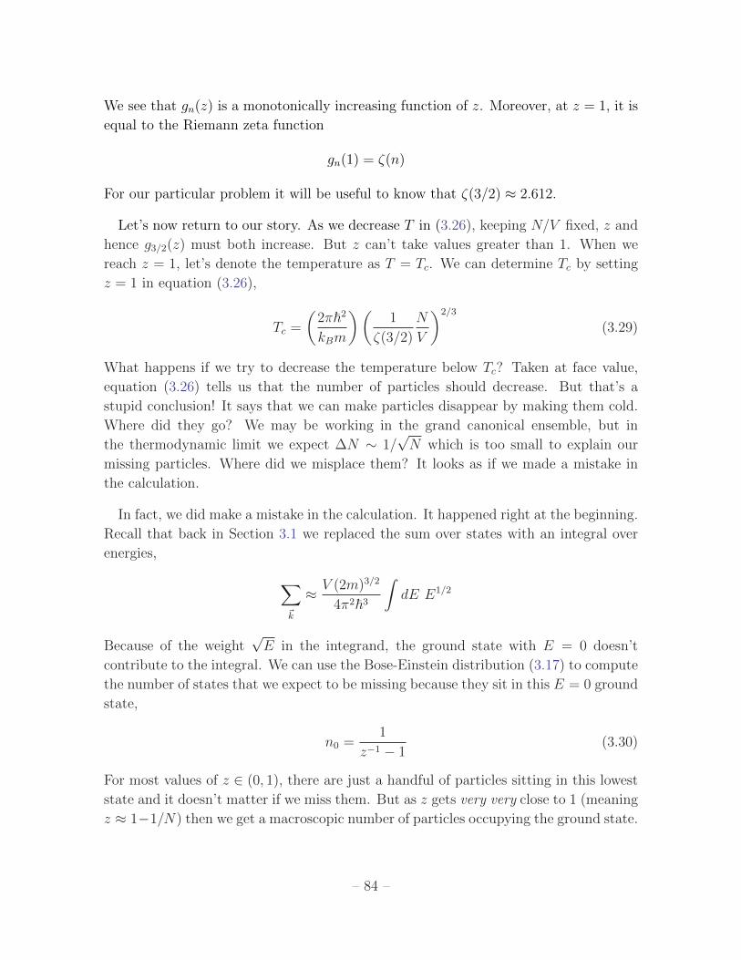
We see that gn(z) is a monotonically increasing function of z. Moreover, at z = 1, it is
equal to the Riemann zeta function
gn(1) = ζ(n)
For our particular problem it will be useful to know that ζ(3/2) ≈ 2.612.
Let’s now return to our story. As we decrease T in (3.26), keeping N/V fixed, z and
hence g3/2(z) must both increase. But z can’t take values greater than 1. When we
reach z = 1, let’s denote the temperature as T = Tc. We can determine Tc by setting
z = 1 in equation (3.26),
Tc =
(2π~2
kBm
)(1
ζ(3/2)
N
V
)2/3
(3.29)
What happens if we try to decrease the temperature below Tc? Taken at face value,
equation (3.26) tells us that the number of particles should decrease. But that’s a
stupid conclusion! It says that we can make particles disappear by making them cold.
Where did they go? We may be working in the grand canonical ensemble, but in
the thermodynamic limit we expect ∆N ∼ 1/√N which is too small to explain our
missing particles. Where did we misplace them? It looks as if we made a mistake in
the calculation.
In fact, we did make a mistake in the calculation. It happened right at the beginning.
Recall that back in Section 3.1 we replaced the sum over states with an integral over
energies,
∑~k
≈ V (2m)3/2
4π2~3
∫dE E1/2
Because of the weight√E in the integrand, the ground state with E = 0 doesn’t
contribute to the integral. We can use the Bose-Einstein distribution (3.17) to compute
the number of states that we expect to be missing because they sit in this E = 0 ground
state,
n0 =1
z−1 − 1(3.30)
For most values of z ∈ (0, 1), there are just a handful of particles sitting in this lowest
state and it doesn’t matter if we miss them. But as z gets very very close to 1 (meaning
z ≈ 1−1/N) then we get a macroscopic number of particles occupying the ground state.
– 84 –

It is a simple matter to redo our calculation taking into account the particles in the
ground state. Equation (3.26) is replaced by
N =V
λ3g3/2(z) +
z
1− z
Now there’s no problem keeping N fixed as we take z close to 1 because the additional
term diverges. This means that if we have finite N , then as we decrease T we can never
get to z = 1. Instead, z must level out around z ≈ 1− 1/N as T → 0.
For T < Tc, the number of particles sitting in the ground state is O(N ). Some simple
algebra allows us to determine that fraction of particles in the ground state is
n0
N= 1− V
Nλ3ζ(3/2) = 1−
(T
Tc
)3/2
(3.31)
At temperatures T < Tc, a macroscopic number of atoms discard their individual
identities and merge into a communist collective, a single quantum state so large that
it can be seen with the naked eye. This is known as the Bose-Einstein condensate. It
provides an exquisitely precise playground in which many quantum phenomena can be
tested.
Bose-Einstein Condensates in the Lab
Bose-Einstein condensates (often shortened to BECs) of
Figure 18: UFO=BEC
weakly interacting atoms were finally created in 1995,
some 70 years after they were first predicted. These first
BECs were formed of Rubidium, Sodium or Lithium
and contained between N ∼ 104 → 107 atoms. The
transition temperatures needed to create these conden-
sates are extraordinarily small, around Tc ∼ 10−7K. Figure 19 shows the iconic colour
enhanced plots that reveal the existence of the condensate. To create these plots, the
atoms are stored in a magnetic trap which is then turned off. A picture is taken of the
atom cloud a short time t later when the atoms have travelled a distance ~kt/m. The
grey UFO-like smudges above are the original pictures. From the spread of atoms, the
momentum distribution of the cloud is inferred and this is what is shown in Figure 19.
The peak that appears in the last two plots reveals that a substantial number of atoms
were indeed sitting in the momentum ground state. (This is not a k = 0 state because
of the finite trap and the Heisenberg uncertainty relation). The initial discoverers of
BECs, Eric Cornell and Carl Wieman from Boulder and Wolfgang Ketterle from MIT,
were awarded the 2001 Nobel prize in physics.
– 85 –
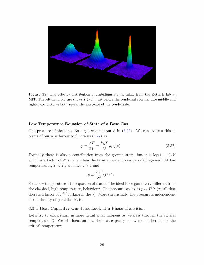
Figure 19: The velocity distribution of Rubidium atoms, taken from the Ketterle lab at
MIT. The left-hand picture shows T > Tc, just before the condensate forms. The middle and
right-hand pictures both reveal the existence of the condensate.
Low Temperature Equation of State of a Bose Gas
The pressure of the ideal Bose gas was computed in (3.22). We can express this in
terms of our new favourite functions (3.27) as
p =2
3
E
V=kBT
λ3g5/2(z) (3.32)
Formally there is also a contribution from the ground state, but it is log(1 − z)/V
which is a factor of N smaller than the term above and can be safely ignored. At low
temperatures, T < Tc, we have z ≈ 1 and
p =kBT
λ3ζ(5/2)
So at low temperatures, the equation of state of the ideal Bose gas is very different from
the classical, high temperature, behaviour. The pressure scales as p ∼ T 5/2 (recall that
there is a factor of T 3/2 lurking in the λ). More surprisingly, the pressure is independent
of the density of particles N/V .
3.5.4 Heat Capacity: Our First Look at a Phase Transition
Let’s try to understand in more detail what happens as we pass through the critical
temperature Tc. We will focus on how the heat capacity behaves on either side of the
critical temperature.
– 86 –

We’ve already seen in (3.32) that we can express the energy in terms of the function
g5/2(z),
E
V=
3
2
kBT
λ3g5/2(z)
so the heat capacity becomes
CVV
=1
V
dE
dT=
15kB4λ3
g5/2(z) +3
2
kBT
λ3
dg5/2
dz
dz
dT(3.33)
The first term gives a contribution both for T < Tc and for T > Tc. However, the second
term includes a factor of dz/dT and z is a very peculiar function of temperature: for
T > Tc, it is fairly smooth, dropping off at T = Tc. However, as T → Tc, the fugacity
rapidly levels off to the value z ≈ 1− 1/N . For T < Tc, z doesn’t change very much at
all. The net result of this is that the second term only contributes when T > Tc. Our
goal here is to understand how this contribution behaves as we approach the critical
temperature.
Let’s begin with the easy bit. Below the critical temperature, T < Tc, only the first
term in (3.33) contributes and we may happily set z = 1. This gives the heat capacity,
CV =15V
4λ3ζ(5/2) ∼ T 3/2 (3.34)
Now we turn to T > Tc. Here we have z < 1, so g5/2(z) < g5/2(1). We also have
dz/dT < 0. This means that the heat capacity decreases for T > Tc. But we know
that for T < Tc, CV ∼ T 3/2 so the heat capacity must have a maximum at T = Tc.
Our goal in this section is to understand a little better what the function CV looks like
in this region.
To compute the second term in (3.33) we need to understand both g′5/2 and how z
changes with T as we approach Tc from above. The first calculation is easy is we use
our expression (3.28),
gn(z) =∞∑m=1
zm
mn⇒ d
dzgn(z) =
1
zgn−1(z) (3.35)
As T → Tc from above, dg5/2/dT → ζ(3/2), a constant. All the subtleties lie in the
remaining term, dz/dT . After all, this is the quantity which is effectively vanishing for
T < Tc. What’s it doing at T > Tc? To figure this out is a little more involved. We
start with our expression (3.26),
g3/2(z) =Nλ3
VT > Tc (3.36)
– 87 –

and we’ll ask what happens to the function g3/2(z) as z → 1, keeping N fixed. We
know that exactly at z = 1, g3/2(1) = ζ(3/2). But how does it approach this value? To
answer this, it is actually simplest to look at the derivative dg3/2/dz = g1/2/z, where
g1/2(z) =1
Γ(1/2)
∫ ∞0
dxx−1/2
z−1ex − 1
The reason for doing this is that g1/2 diverges as z → 1 and it is generally easier to
isolate divergent parts of a function than some finite piece. Indeed, we can do this
straightforwardly for g1/2 by looking at the integral very close to x = 0, we can write
g1/2(z) =1
Γ(1/2)
∫ ε
0
dxx−1/2
z−1(1 + x)− 1+ finite
=z
Γ(1/2)
∫ ε
0
dxx−1/2
(1− z) + x+ . . .
=2z√1− z
1
Γ(1/2)
∫ ε
0
du1
1 + u2+ . . .
where, in the last line, we made the substution u =√x/(1− z). So we learn that
as z → 1, g1/2(z) → z(1 − z)−1/2. But this is enough information to tell us how g3/2
approaches its value at z = 1: it must be
g3/2(z) ≈ ζ(3/2) + A(1− z)1/2 + . . .
for some constant A. Inserting this into our equation (3.36) and rearranging, we find
that as T → Tc from above,
z ≈ 1− 1
A2
(ζ(3/2)− Nλ3
V
)2
= 1− ζ(3/2)2
A2
((T
Tc
)3/2
− 1
)2
≈ 1−B(T − TcTc
)2
where, in the second line, we used the expression of the critical temperature (3.29).
B is some constant that we could figure out with a little more effort, but it won’t be
important for our story. From the expression above, we can now determine dz/dT as
T → Tc. We see that it vanishes linearly at T = Tc.
– 88 –

Putting all this together, we can determine the expression for the heat capacity
(3.33) when T > Tc. We’re not interested in the coefficients, so we’ll package a bunch
of numbers of order 1 into a constant b and the end result is
CV =15V kB
4λ3g5/2(z)− b
(T − TcTc
)The first term above goes smoothly over to the
CV
T
TC
3Nk /2B
Figure 20: Heat Capacity for a BEC
expression (3.34) for CV when T < Tc. But
the second term is only present for T > Tc.
Notice that it goes to zero as T → Tc, which
ensures that the heat capacity is continuous at
this point. But the derivative is not continu-
ous. A sketch of the heat capacity is shown in
the figure.
Functions in physics are usually nice and
smooth. How did we end up with a discontinuity in the derivative? In fact, if we
work at finite N , strictly speaking everything is nice and smooth. There is a similar
contribution to dz/dT even at T < Tc. We can see that by looking again at the
expressions (3.30) and (3.31), which tell us
z =
(1 +
1
n0
)−1
=
(1 +
1
N
1
1− (T/Tc)3/2
)−1
(T < Tc)
The difference is that while dz/dT is of order one above Tc, it is of order 1/N below
Tc. In the thermodynamic limit, N →∞, this results in the discontinuity that we saw
above. This is a general lesson: phase transitions with their associated discontinuities
can only arise in strictly infinite systems. There are no phase transitions in finite
systems.
Superfluid Helium-4
A similar, but much more pronounced, discontinuity is seen in Helium-4 as it
becomes a superfluid, a transition which occurs at 2.17 K. The atom contains two
protons, two neutrons and two electrons and is therefore a boson. (In contrast, Helium-
3 contains just a single neutron and is a fermion). The experimental data for the heat
capacity of Helium-4 is shown on the right. The successive graphs are zooming in
on the phase transistion: the scales are (from left to right) Kelvin, milliKelvin and
microKelvin. The discontinuity is often called the lambda transition on account of the
shape of this graph.
– 89 –

There is a close connection between Bose-
Figure 21: 4He.
Einstein condensation described above and su-
perfluids: strictly speaking a non-interacting Bose-
Einstein condensate is not a superfluid but su-
perfluidity is a consequence of arbitrarily weak
repulsive interactions between the atoms. How-
ever, in He-4, the interactions between atoms
are strong and the system cannot be described
using the simple techniques developed above.
Something very similar to Bose condensation
also occurs in superconductivity and superfluidity of Helium-3. Now the primary char-
acters are fermions rather than bosons (electrons in the case of superconductivity). As
we will see in the next section, fermions cannot condense. But they may form bound
states due to interactions and these effective bosons can then undergo condensation.
3.6 Fermions
For our final topic, we will discuss the fermion gases. Our analysis will focus solely
on non-interacting fermions. Yet this simple model provides a (surprisingly) good
first approximation to a wide range of systems, including electrons in metals at low
temperatures, liquid Helium-3 and white dwarfs and neutron stars.
Fermions are particles with 12-integer spin. By the spin-statistics theorem, the wave-
function of the system is required to pick up a minus sign under exchange of any
particle,
ψ(~r1, ~r2) = −ψ(~r2, ~r1)
As a corollory, the wavefunction vanishes if you attempt to put two identical fermions
in the same place. This is a reflection of the Pauli exclusion principle which states that
fermions cannot sit in the same state. We will see that the low-energy physics of a gas
of fermions is entirely dominated by the exclusion principle.
We work again in the grand canonical ensemble. The grand partition function for a
single state |r〉 is very easy: the state is either occupied or it is not. There is no other
option.
Zr =∑n=0,1
e−βn(Er−µ) = 1 + e−β(Er−µ)
– 90 –
So, the grand partition function for all states is Z =∏
r Zr, from which we can compute
the average number of particles in the system
N =∑r
1
eβ(Er−µ) + 1≡∑r
nr
where the average number of particles in the state |r〉 is
nr =1
eβ(Er−µ) + 1(3.37)
This is the Fermi-Dirac distribution. It differs from the Bose-Einstein distribution only
by the sign in the denominator. Note however that we had no convergence issues in
defining the partition function. Correspondingly, the chemical potential µ can be either
positive or negative for fermions.
3.6.1 Ideal Fermi Gas
We’ll look again at non-interacting, non-relativistic particles with E = ~2k2/2m . Since
fermions necessarily have 12-integer spin, s, there is always a degeneracy factor when
counting the number of states given by
gs = 2s+ 1
For example, electrons have spin 12
and, correspondingly have a degeneracy of gs = 2
which just accounts for “spin up” and “spin down” states. We saw similar degeneracy
factors when computing the density of states for photons (which have two polarizations)
and phonons (which had three). For non-relativistic fermions, the density of states is
g(E) =gsV
4π2
(2m
~2
)3/2
E1/2
We’ll again use the notation of fugacity, z = eβµ. The particle number is
N =
∫dE
g(E)
z−1eβE + 1(3.38)
The average energy is
E =
∫dE
Eg(E)
z−1eβE + 1
And the pressure is
pV =1
β
∫dE g(E) log
(1 + ze−βE
)=
2
3E (3.39)
– 91 –

At high temperatures, it is simple to repeat the steps of Section 3.5.2. (This is one of
the questions on the problem sheet). Ony a few minus signs differ along the way and
one again finds that for z 1, the equation of state reduces to that of a classical gas,
pV = NkBT
(1 +
λ3N
4√
2gsV+ . . .
)(3.40)
Notice that the minus signs filter down to the final answer: the first quantum correction
to a Fermi gas increases the pressure.
3.6.2 Degenerate Fermi Gas and the Fermi Surface
In the extreme limit T → 0, the Fermi-Dirac distribution becomes very simple: a state
is either filled or empty.
1
eβ(E−µ) + 1−→
1 for E < µ
0 for E > µ
It’s simple to see what’s going on here. Each fermion that we throw into the system
settles into the lowest available energy state. These are successively filled until we run
out of particles. The energy of the last filled state is called the Fermi energy and is
denoted as EF . Mathematically, it is the value of the chemical potential at T = 0,
µ(T = 0) = EF (3.41)
Filling up energy states with fermions is just like throwing balls into a box. With one
exception: the energy states of free particles are not localised in position space; they
are localised in momentum space. This means that successive fermions sit in states
with ever-increasing momentum. In this way, the fermions fill out a ball in momentum
space. The momentum of the final fermion is called the Fermi momentum and is related
to the Fermi energy in the usual way: ~kF = (2mEF )1/2. All states with wavevector
|~k| ≤ kF are filled and are said to form the Fermi sea or Fermi sphere. Those states
with |~k| = kF lie on the edge of the Fermi sea. They are said to form the Fermi
surface. The concept of a Fermi surface is extremely important in later applications to
condensed matter physics.
We can derive an expression for the Fermi energy in terms of the number of particles
N in the system. To do this, we should appreciate that we’ve actually indulged in a
slight abuse of notation when writing (3.41). In the grand canonical ensemble, T and
µ are independent variables: they’re not functions of each other! What this equation
really means is that if we want to keep the average particle number N in the system
– 92 –

fixed (which we do) then as we vary T we will have to vary µ to compensate. So a
slightly clearer way of defining the Fermi energy is to write it directly in terms of the
particle number
N =
∫ EF
0
dE g(E) =gsV
6π2
(2m
~2
)3/2
E3/2F (3.42)
Or, inverting,
EF =~2
2m
(6π2
gs
N
V
)2/3
(3.43)
The Fermi energy sets the energy scale for the system. There is an equivalent tem-
perature scale, TF = EF/kB. The high temperature expansion that resulted in the
equation of state (3.40) is valid at temperatures T > TF . In contrast, temperatures
T < TF are considered “low” temperatures for systems of fermions. Typically, these
low temperatures do not have to be too low: for electrons in a metal, TF ∼ 104K; for
electrons in a white dwarf, TF > 107K.
While EF is the energy of the last occupied state, the average energy of the system
can be easily calculated. It is
E =
∫ EF
0
dE Eg(E) =3
5NEF (3.44)
Similarly, the pressure of the degenerate Fermi gas can be computed using (3.39),
pV =2
5NEF (3.45)
Even at zero temperature, the gas has non-zero pressure, known as degeneracy pressure.
It is a consequence of the Pauli exclusion principle and is important in the astrophysics
of white dwarf stars and neutron stars. (We will describe this application in Section
3.6.5). The existence of this residual pressure at T = 0 is in stark contrast to both the
classical ideal gas (which, admittedly, isn’t valid at zero temperature) and the bosonic
quantum gas.
3.6.3 The Fermi Gas at Low Temperature
We now turn to the low-temperature behaviour of the Fermi gas. As mentioned above,
“low” means T TF , which needn’t be particularly low in everyday terms. The
number of particles N and the average energy E are given by,
N =
∫ ∞0
dEg(E)
z−1eβE + 1(3.46)
– 93 –

FE
FET=0n(E)
1
E
T <<
Figure 22: The Fermi-Dirac Distribution function at T = 0 and very small T . The distri-
bution differs from the T = 0 ground state only for a range of energies kBT around EF .
and
E =
∫ ∞0
dEEg(E)
z−1eβE + 1(3.47)
where, for non-relativistic fermions, the density of states is
g(E) =gsV
4π2
(2m
~2
)3/2
E1/2
Our goal is to firstly understand how the chemical potential µ, or equivalently the
fugacity z = eβµ, changes with temperature when N is held fixed. From this we can
determine how E changes with temperature when N is held fixed.
There are two ways to proceed. The first is a direct approach on the problem by
Taylor expanding (3.46) and (3.47) for small T . But it turns out that this is a little
delicate because the starting point at T = 0 involves the singular distribution shown
on the left-hand side of Figure 22 and it’s easy for the physics to get lost in a morass of
integrals. For this reason, we start by developing a heuristic understanding of how the
integrals (3.46) and (3.47) behave at low temperatures which will be enough to derive
the required results. We will then give the more rigorous expansion – sometimes called
the Sommerfeld expansion – and confirm that our simpler derivation is indeed correct.
The Fermi-Dirac distribution (3.37) at small temperatures is sketched on the right-
hand side of Figure 22. The key point is that only states with energy within kBT of
the Fermi surface are affected by the temperature. We want to insist that as we vary
the temperature, the number of particles stays fixed which means that dN/dT = 0.
I claim that this holds if, to leading order, the chemical potential is independent of
temperature, so
dµ
dT
∣∣∣∣T=0
= 0 (3.48)
– 94 –

Let’s see why this is the case. The change in particle number can be written as
dN
dT=
d
dT
∫ ∞0
dEg(E)
eβ(E−µ) + 1
=
∫ ∞0
dE g(E)d
dT
(1
eβ(E−µ) + 1
)≈ g(EF )
∫ ∞0
dE∂
∂T
(1
eβ(E−EF ) + 1
)There are two things going on in the step from the second line to the third. Firstly,
we are making use of the fact that, for kBT EF , the Fermi-Dirac distribution
only changes significantly in the vicinity of EF as shown in the right-hand side of
Figure 22. This means that the integral in the middle equation above is only receiving
contributions in the vicinity of EF and we have used this fact to approximate the density
of states g(E) with its value at g(EF ). Secondly, we have used our claimed result (3.48)
to replace the total derivative d/dT (which acts on the chemical potential) with the
partial derivative ∂/∂T (which doesn’t) and µ is replaced with its zero temperature
value EF .
Explicitly differentiating the Fermi-Dirac distribution in the final line, we have
dN
dT≈ g(EF )
∫ ∞0
dE
(E − EFkBT 2
)1
4 cosh2(β(E − EF )/2)≈ 0
This integral vanishes because (E − EF ) is odd around EF while the cosh function
is even. (And, as already mentioned, the integral only receives contributions in the
vicinity of EF ).
Let’s now move on to compute the change in energy with temperature. This, of
course, is the heat capacity. Employing the same approximations that we made above,
we can write
CV =∂E
∂T
∣∣∣∣N,V
=
∫ ∞0
dE Eg(E)∂
∂T
(1
eβ(E−µ) + 1
)≈∫ ∞
0
dE
[EFg(EF ) +
3
2g(EF )(E − Ef )
]∂
∂T
(1
eβ(E−EF ) + 1
)However, this time we have not just replaced Eg(E) by EFg(EF ), but instead Taylor
expanded to include a term linear in (E−EF ). (The factor of 3/2 comes about because
Eg(E) ∼ E3/2. The first EFg(EF ) term in the square brackets vanishes by the same
even/odd argument that we made before. But the (E − EF ) term survives.
– 95 –

Writing x = β(E − EF ), the integral becomes
CV ≈3
2g(EF )T
∫ ∞−∞
dxx2
4 cosh2(x/2)
where we’ve extended the range of the integral from −∞ to +∞, safe in the knowledge
that only the region near EF (or x = 0) contributes anyway. More importantly, how-
ever, this integral only gives an overall coefficient which we won’t keep track of. The
final result for the heat capacity is
CV ∼ T g(EF )
There is a simple way to intuitively understand this linear behaviour. At low temper-
atures, only fermions within kBT of EF are participating in the physics. The number
of these particles is ∼ g(EF )kBT . If each picks up energy ∼ kBT then the total energy
of the system scales as E ∼ g(EF )(kBT )2, resulting in the linear heat capacity found
above.
Finally, the heat capacity is often re-expressed in a slightly different form. Using
(3.42) we learn that N ∼ E3/2F which allows us to write,
CV ∼ NkB
(T
TF
)(3.49)
Heat Capacity of Metals
One very important place that we can apply the theory above it to metals. We can try
to view the conduction electrons — those which are free to move through the lattice
— as an ideal gas. At first glance, this seems very unlikely to work. This is because we
are neglecting the Coulomb interaction between electrons. Nonetheless, the ideal gas
approximation for electrons turns out to work remarkably well.
From what we’ve learned in this section, we would expect two contributions to the
heat capacity of a metal. The vibrations of the lattice gives a phonon contribution
which goes as T 3 (see equation (3.13)). If the conduction electrons act as an ideal gas,
they should give a linear term. The low-temperature heat capacity can therefore be
written as
CV = γT + αT 3
Experimental data is usually plotted as CV /T vs T 2 since this gives a straight line
which looks nice. The intercept with the CV axis tells us the electron contribution.
The heat capacity for copper is shown in the figure.
– 96 –

We can get a rough idea of when the phonon and
Figure 23: The heat capacity
of copper (taken from A. Tari
“The Specific Heat of Matter at
Low Temperatures”)
electron contributions to heat capacity are compara-
ble. Equating (3.14) with (3.56), and writing 24π2/5 ≈50, we have the the two contributions are equal when
T 2 ∼ T 3D/50TF . Ballpark figures are TD ∼ 102K and
TF ∼ 104K which tells us that we have to get down
to temperatures of around 1K or so to see the electron
contribution.
For many metals, the coefficient γ of the linear heat
capacity is fairly close to the ideal gas value (within,
say, 20% or so). Yet the electrons in a metal are far
from free: the Coulomb energy from their interations
is at least as important as the kinetic energy. So why
does the ideal gas approximation work so well? This was explained in the 1950s by
Landau and the resulting theory — usually called Landau’s Fermi liquid theory — is
the basis for our current understanding of electron systems.
3.6.4 A More Rigorous Approach: The Sommerfeld Expansion
The discussion in Section 3.6.3 uses some approximations but highlights the physics
of the low-temperature fermi gas. For completeness, here we present a more rigorous
derivation of the low-temperature expansion.
To start, we introduce some new notation for the particle number and energy inte-
grals, (3.46) and (3.47). We write,
N
V=
gs4π2
(2m
~2
)3/2 ∫ ∞0
dEE1/2
z−1eβE + 1
=gsλ3f3/2(z) (3.50)
and
E
V=
gs4π2
(2m
~2
)3/2 ∫ ∞0
dEE3/2
z−1eβE + 1
=3
2
gsλ3kBT f5/2(z) (3.51)
where λ =√
2π~2/mkBT is the familiar thermal wavelength and the functions fn(z)
are the fermionic analogs of gn defined in (3.27),
fn(z) =1
Γ(n)
∫ ∞0
dxxn−1
z−1ex + 1(3.52)
– 97 –
where it is useful to recall Γ(3/2) =√π/2 and Γ(5/2) = 3
√π/4 (which follows, of
course, from the property Γ(n + 1) = nΓ(n)). This function is an example of a poly-
logarithm and is sometimes written as Lin(−z) = −fn(z).
Expanding fn(z)
We will now derive the large z expansion of fn(z), sometimes called the Sommerfeld
expansion. The derivation is a little long. We begin by splitting the dx integral into
two parts,
Γ(n)fn(z) =
∫ βµ
0
dxxn−1
z−1ex + 1+
∫ ∞βµ
dxxn−1
z−1ex + 1
=
∫ βµ
0
dx xn−1
(1− 1
1 + ze−x
)+
∫ ∞βµ
dxxn−1
z−1ex + 1
=(log z)n
n−∫ βµ
0
dxxn−1
1 + ze−x+
∫ ∞βµ
dxxn−1
z−1ex + 1
We now make a simple change of variable, η1 = βµ − x for the first integral and
η2 = x− βµ for the second,
Γ(n)fn(z) =(log z)n
n−∫ βµ
0
dη1(βµ− η1)n−1
1 + eη1+
∫ ∞0
dη2(βµ+ η2)n−1
1 + eη2
So far we have only massaged the integral into a useful form. We now make use of the
approximation βµ 1. Firstly, we note that the first integral has a eη1 suppression
in the denominator. If we replace the upper limit of the integral by ∞, the expression
changes by a term of order e−βµ = z−1 which is a term we’re willing to neglect. With
this approximation, we can combine the two integrals into one,
Γ(n)fn(z) =(log z)n
n+
∫ ∞0
dη(βµ+ η)n−1 − (βµ− η)n−1
1 + eη
We now Taylor expand the numerator,
(βµ+ η)n−1 − (βµ− η)n−1 = (βµ)n−1[(1 + η/βµ)n−1 − (1− η/βµ)n−1
]= (βµ)n−1
[1 + (n− 1)
η
βµ+ . . .− 1 + (n− 1)
η
βµ+ . . .
]= 2(n− 1)(βµ)n−2η + . . .
From which we get
Γ(n)fn(z) =(log z)n
n+ 2(n− 1)(log z)n−2
∫ ∞0
dηη
eη + 1
– 98 –

We’re left with a fairly simple integral.∫ ∞0
dηη
eη + 1=
∫ ∞0
dηηe−η
1 + e−η
=
∫ ∞0
dη η
∞∑m=1
e−mη(−1)m+1
=∞∑m=1
(−1)m+1
m2
∫ ∞0
du ue−u
The integral in the last line is very simple:∫∞
0du ue−u = 1. We have only to do the
sum. There are a number of ways to manipulate this. We chose to write
1− 1
22+
1
32− 1
42. . . =
(1 +
1
22+
1
32+
1
42+ . . .
)− 2
(1
22+
1
42+
1
62+ . . .
)=
(1− 2
22
)·(
1 +1
22+
1
32+ . . .
)(3.53)
This final sum is well known. It is∑
1/m2 = ζ(2) = π2/6. (The original proof of this,
by Euler, proceeds by Taylor expanding sin x/x, writing resulting sum as a product of
roots, and then equating the x2 term).
After all this work, we finally have the result we want. The low temperature expan-
sion of fn(z) is an expansion in 1/ log z = 1/βµ,
fn(z) =(log z)n
Γ(n+ 1)
(1 +
π2
6
n(n− 1)
(log z)2+ . . .
)(3.54)
Back to Physics: Heat Capacity of a Fermi Gas Again
The expansion (3.54) is all we need to determine the leading order effects of temperature
on the Fermi gas. The number of particles (3.50) can be expressed in terms of the
chemical potential as
N
V=
gs6π2~3
(2mµ)3/2
(1 +
π2
8
(kBT
µ
)2
+ . . .
)(3.55)
But the number of particles determines the Fermi energy through (3.43). For fixed
particle numberN , we can therefore express the chemical potential at finite temperature
in terms of the Fermi energy. After a small amount of algebra, we find
µ = EF
(1− π2
12
(kBT
EF
)2
+ . . .
)
– 99 –

We see that the chemical potential is a maximum at T = 0 and decreases at higher
T . This is to be expected: recall that by the time we get to the classical gas, the
chemical potential must be negative. Moreover, note that the leading order correction
is quadratic in temperature rather than linear, in agreement with our earlier claim
(3.48).
The energy density can be computed from (3.51) and (3.54). It is
E
V=
gs10π2~3
(2m)3/2µ5/2
(1 +
5π2
8
(kBT
µ
)2
+ . . .
)Our real interest is in the heat capacity. However, with fixed particle number N , the
chemical potential also varies with temperature at quadratic order. We can solve this
problem by dividing by (3.55) to get
E
N=
3EF5
(1 +
5π2
12
(kBT
EF
)2
+ . . .
)Now the only thing that depends on temperature on the right-hand side is T itself.
From this we learn that the heat capacity of a low temperature Fermi gas is linear in
T ,
CV =∂E
∂T
∣∣∣∣N,V
= NkBπ2
2
T
TF(3.56)
But we now have the correct coefficient that completes our earlier result (3.49).
3.6.5 White Dwarfs and the Chandrasekhar limit
When stars exhaust their fuel, the temperature T → 0 and they have to rely on the Pauli
exclusion principle to support themselves through the degeneracy pressure (3.45). Such
stars supported by electron degeneracy pressure are called white dwarfs. In addition
to the kinetic energy Ekinetic of fermions given in (3.43) the system has gravitational
energy. If we make the further assumption that the density in a star of radius R is
uniform, then
Egrav = −3
5
GNM2
Rwhere GN is Newton’s constant. In the problem set, you will minimise Egrav + Ekinetic
to find the relationship between the radius and mass of the star,
R ∼M−1/3
This is unusual. Normally if you throw some stuff on a pile, the pile gets bigger. Not
so for stars supported by degeneracy pressure. The increased gravitational attraction
wins and causes them to shrink.
– 100 –

As the star shrinks, the Fermi energy (3.43) grows. Eventually it becomes comparable
to the electron massme and our non-relativistic approximation breaks down. We can re-
do our calculations using the relativistic formula for the density of states (3.4) (which
needs to be multiplied by a factor of 2 to account for the spin degeneracy). In the
opposite regime of ultra-relativistic electrons, where E me, then we can expand the
density of states as
g(E) =V
π2~3c3
(E2 − m2c4
2+ . . .
)from which we can determine the kinetic energy due to fermions, replacing the non-
relativistic result (3.44) by
Ekinetic =V
π2~3c3
(1
4E4F −
m2c4
4E2F + . . .
)The Fermi energy can be expressed in terms of the particle number by
N =V
π2~3c3
(1
3E3F −
m2c4
2EF + . . .
)The total energy of the system is then given by,
Egrav + EF =
[3~c4
(9πM4
4m4p
)1/3
− 3
5GNM
2
]1
R+O(R)
where mp is the proton mass (and we’re taking M = Nmp as a good approximation
to the full mass of the star). If the term above is positive then the star once again
settles into a minimum energy state, where the 1/R term balances the term that grows
linearly in R. But if the 1/R term is negative, we have a problem: the star is unstable
to gravitational collapse and will shrink to smaller and smaller values of R. This occurs
when the mass exceeds the Chandrasekhar limit, M > MC . Neglecting factors of 2 and
π, this limit is
MC ∼(
~cGN
)3/21
m2p
(3.57)
This is roughly 1.5 times the mass of the Sun. Stars that exceed this bound will not
end their life as white dwarfs. Their collapse may ultimately be stopped by degeneracy
pressure of neutrons so that they form a neutron star. Or it may not be stopped at all
in which case they form a black hole.
– 101 –

The factor in brackets in (3.57) is an interesting mix of fundamental constants as-
sociated to quantum theory, relativity and gravity. In this combination, they define a
mass scale called the Planck mass,
M2pl =
~cGN
When energy densities reach the Planck scale, quantum gravity effects are important
meaning that we have to think of quantising spacetime itself. We haven’t quite reached
this limit in white dwarf stars. (We’re shy by about 25 orders of magnitude or so!).
Nonetheless the presence of the Planck scale in the Chandra limit is telling us that
both quantum effects and gravitational effects are needed to understand white dwarf
stars: the matter is quantum; the gravity is classical.
3.6.6 Pauli Paramagnetism
“With heavy heart, I have decided that Fermi-Dirac, not Einstein, is the
correct statistics, and I have decided to write a short note on paramag-
netism”
Wolfgang Pauli, in a letter to Schrodinger, reluctantly admitting that elec-
trons are fermions
We now describe a gas of electrons in a background magnetic field ~B. There are
two effects that are important: the Lorentz force ~v × B on the motion of electrons
and the coupling of the electron spin to the magnetic field. We first discuss the spin
coupling and postpone the Lorentz force for the next section.
An electron can have two spin states, “up” and “down”. We’ll denote the spin state
by a discrete label: s = 1 for spin up; s = −1 for spin down. In a background magnetic
field ~B, the kinetic energy picks up an extra term
Espin = µBBs (3.58)
where µB = |e|~/2m is the Bohr magneton. (It has nothing to do with the chemical
potential. Do not confuse them!)
Since spin up and spin down electrons have different energies, their occupation num-
bers differ. Equation (3.50) is now replaced by
N↑V
=1
4π2
(2m
~2
)3/2 ∫ ∞0
dEE1/2
eβ(E+µBB−µ) + 1=
1
λ3f3/2(ze−βµBB)
N↓V
=1
4π2
(2m
~2
)3/2 ∫ ∞0
dEE1/2
eβ(E−µBB−µ) + 1=
1
λ3f3/2(ze+βµBB)
– 102 –

Our interest is in computing the magnetization, which is a measure of how the energy
of the system responds to a magnetic field,
M = −∂E∂B
(3.59)
Since each spin has energy (3.58), the magnetization is simply the difference in the in
the number of up spins and down spins,
M = −µB(N↑ −N↓) = −µBVλ3
[f3/2(ze−βµBB)− f3/2(zeβµBB)
]At high temperatures, and suitably low magnetic fields, we can approximate f3/2(z) ≈ z
as z → 0, so that
M ≈ 2µBV z
λ3sinh(βµBB)
We can eliminate the factor of z in favour of the particle number,
N = N↑ +N↓ ≈2V z
λ3cosh(βµBB)
From which we can determine the high temperature magnetization,
M ≈ µBN tanh(βµBB)
This is the same result that you computed in the first problem sheet using the simple
two-state model. We see that, once again, at high temperatures the quantum statistics
are irrelevant. The magnetic susceptibility is a measure of how easy it is to magnetise
a substance. It is defined as
χ ≡ ∂M
∂B(3.60)
Evaluating χ in the limit of vanishing magnetic field, we find that the magnetization
is inversely proportional to the temperature,
χ(B = 0) =Nµ2
B
kBT
This 1/T behaviour is known as Curie’s law. (Pierre, not Marie).
– 103 –

The above results hold in the high temperature limit. In contrast, at low tempera-
tures the effects of the Fermi surface become important. We need only keep the leading
order term in (3.54) to find
M ≈ µBV
6π2
(2m
~2
)3/2 [(EF + µBB)3/2 − (EF − µBB)3/2
]≈ µ2
BV
2π2
(2m
~2
)3/2
E1/2F B
where we’re written the final result in the limit µBB EF and expanded to linear order
in B. We could again replace some of the factors for the electron number N . However,
we can emphasise the relevant physics slightly better if we write the result above in
terms of the density of states (3.19). Including the factor of 2 for spin degeneracy, we
have
M ≈ µ2Bg(EF )B (3.61)
We see that at low temperatures, the magnetic susceptibility no longer obeys Curie’s
law, but saturates to a constant
χ ≡ ∂M
∂B= µ2
Bg(EF )
What’s happening here is that most electrons are embedded deep within the Fermi
surface and the Pauli exclusion principle forbids them from flipping their spins in re-
sponse to a magnetic field. Only those electrons that sit on the Fermi surface itself —
all g(EF ) of them — have the luxury to save energy by aligning their spins with the
magnetic field.
Notice that χ > 0. Such materials are called paramagnetic: in the presence of a
magnetic field, the magnetism increases. Materials that are paramagnetic are attracted
to applied magnetic fields. The effect described above is known as Pauli paramagnetism.
3.6.7 Landau Diamagnetism
For charged fermions, such as electrons, there is a second consequence of placing them
in a magnetic field: they move in circles. The Hamiltonian describing a particle of
charge −e in a magnetic field ~B = ∇× ~A is,
H =1
2m
(~p+ e ~A(~r)
)2
This has an immediate consequence: a magnetic field cannot affect the statistical
physics of a classical gas! This follows simply from substituting the above Hamiltonian
into the classical partition function (2.1). A simple shift of variables, ~p′ = ~p+e ~A shows
that the classical partition function does not depend on ~B. This result (which was also
mentioned in a slightly different way in the Classical Dynamics course) is known as the
Bohr-van Leeuwen theorem: it states that there can be no classical magnetism.
– 104 –

Let’s see how quantum effects change this conclusion. Our first goal is to understand
the one-particle states for an electron in a constant background magnetic field. This is
a problem that you will also solve in the Applications of Quantum Mechanics course.
It is the problem of Landau levels.
Landau Levels
We will consider an electron moving in a constant magnetic field pointing in the z
direction: ~B = (0, 0, B). There are many different ways to pick ~A such that ~B = ∇× ~A
gives the right magnetic field. These are known as gauge choices. Each choice will give
rise to the same physics but, usually, very different equations in the intervening steps.
Here we make the following gauge choice,
~A = (−By, 0, 0) (3.62)
Let’s place our particle in a cubic box with sides of length L. Solutions to the
Schrodinger equation Hψ = Eψ are simply plane waves in the x and z directions,
ψ(~r) = ei(kxx+kzz)f(y)
But the wavefunction f(y) must satisfy,[− ~2
2m
∂2
∂y2+
1
2m(~kx − eBy)2
]f(y) = E ′f(y) (3.63)
But this is a familiar equation! If we define the cyclotron frequency,
ωc =eB
m
Then we can rewrite (3.63) as[− ~2
2m
∂2
∂y2+
1
2mω2
c (y − y0)2
]f(y) = E ′f(y)
where y0 = ~kx/eB. This is simply the Schrodinger equation for a harmonic oscillator,
jiggling with frequency ωc and situated at position y0.
One might wonder why the harmonic oscillator appeared. The cyclotron frequency
ωc is the frequency at which electrons undergo classical Larmor orbits, so that kind of
makes sense. But why have these become harmonic oscillators sitting at positions y0
which depend on kx? The answer is that there is no deep meaning to this at all! it is
merely an artefact of our gauge choice (3.62). Had we picked a different ~A giving rise to
– 105 –

the same ~B, we would find ourselves trying to answer a different question! The lesson
here is that when dealing with gauge potentials, the intermediate steps of a calculation
do not always have physical meaning. Only the end result is important. Let’s see what
this is. The energy of the particle is
E = E ′ +~2k2
z
2m
where E ′ is the energy of the harmonic oscillator,
E ′ =
(n+
1
2
)~ωc n ∈ Z
These discrete energy levels are known as Landau levels. They are highly degenerate.
To see this, note that kx is quantized in unit of ∆kx = 2π/L. This means that we
can have a harmonic oscillator located every ∆y0 = 2π~/eBL. The number of such
oscillators that we can fit into the box of size L is L/∆y0. This is the degeneracy of
each level,
eBL2
2π~≡ Φ
Φ0
where Φ = L2B is the total flux through the system and Φ0 = 2π~/e is known as the
flux quantum. (Note that the result above does not include a factor of 2 for the spin
degeneracy of the electron).
Back to the Diamagnetic Story
We can now compute the grand partition function for non-interacting electrons in a
magnetic field. Including the factor of 2 from electron spin, we have
logZ =L
2π
∫dkz
∞∑n=0
2L2B
Φ0
log
[1 + z exp
(−β~
2k2z
2m− β~ωc(n+ 1/2)
)]To perform the sum, we use the Euler summation formula which states that for any
function h(x),
∞∑n=0
h(n+ 1/2) =
∫ ∞0
h(x)dx+1
24h′(0) + . . .
We’ll apply the Euler summation formula to the function,
h(x) =
∫dkz log
[1 + exp
(−β~
2k2z
2m+ βx
)]
– 106 –

So the grand partition function becomes
logZ =V B
πΦ0
∞∑n=0
h(µ− ~ωc(n+ 1/2))
=V B
πΦ0
∫ ∞0
h(µ− ~ωcx) dx− V B
πΦ0
~ωc24
dh(µ)
dµ+ . . .
=V m
2π2~2
[∫ µ
−∞h(y) dy − (~ωc)2
24
∫ +∞
−∞dk
β
eβ(~2k2/2m−µ) + 1
]+ . . . (3.64)
The first term above does not depend on B. In fact it is simply a rather perverse way
of writing the partition function of a Fermi gas when B = 0. However, our interest
here is in the magnetization which is again defined as (3.59). In the grand canonical
ensemble, this is simply
M =1
β
∂logZ∂B
The second term in (3.64) is proportional to B2 (which is hiding in the ω2c term).
Higher order terms in the Euler summation formula will carry higher powers of B and,
for small B, the expression above will suffice.
At T = 0, the integrand is simply 1 for |k| < kF and zero otherwise. To compare
to Pauli paramagnetism, we express the final result in terms of the Bohr magneton
µB = |e|~/2mc. We find
M = −µ2B
3g(EF )B
This is comparable to the Pauli contribution (3.61). But it has opposite sign. Sub-
stances whose magnetization is opposite to the magnetic field are called diamagnetic:
they are repelled by applied magnetic fields. The effect that we have derived above is
known as Landau diamagnetism.
– 107 –

4. Classical Thermodynamics
“Thermodynamics is a funny subject. The first time you go through it, you
don’t understand it at all. The second time you go through it, you think
you understand it, except for one or two small points. The third time you
go through it, you know you don’t understand it, but by that time you are
used to it, so it doesn’t bother you any more.”
Arnold Sommerfeld, making excuses
So far we’ve focussed on a statistical mechanics, studying systems in terms of
their microscopic constituents. In this section, we’re going to take a step back and
look at classical thermodynamics. This is a theory that cares nothing for atoms and
microscopics. Instead it describes relationships between the observable macroscopic
phenomena that we see directly.
In some sense, returning to thermodynamics is a retrograde step. It is certainly not
as fundamental as the statistical description. Indeed, the “laws” of thermodynamics
that we describe below can all be derived from statistical physics. Nonetheless, there
are a number of reasons for developing classical thermodynamics further.
First, pursuing classical thermodynamics will give us a much deeper understanding
of some of the ideas that briefly arose in Section 1. In particular, we will focus on
how energy flows due to differences in temperature. Energy transferred in this way is
called heat. Through a remarkable series of arguments involving heat, one can deduce
the existence of a quantity called entropy and its implications for irreversibility in
the Universe. This definition of entropy is entirely equivalent to Boltzmann’s later
definition S = kB log Ω but makes no reference to the underlying states.
Secondly, the weakness of thermodynamics is also its strength. Because the theory
is ignorant of the underlying nature of matter, it is limited in what it can tell us.
But this means that the results we deduce from thermodynamics are not restricted to
any specific system. They will apply equally well in any circumstance, from biological
systems to quantum gravity. And you can’t say that about a lot of theories!
In Section 1, we briefly described the first and second laws of thermodynamics as
consequences of the underlying principles of statistical physics. Here we instead place
ourselves in the shoes of Victorian scientists with big beards, silly hats and total igno-
rance of atoms. We will present the four laws of thermodynamics as axioms on which
the theory rests.
– 108 –

4.1 Temperature and the Zeroth Law
We need to start with a handful of definitions:
• A system that is completely isolated from all outside influences is said to be
contained in adiabatic walls. We will also refer to such systems as insulated.
• Walls that are not adiabatic are said to be diathermal and two systems separated
by a diathermal wall are said to be in thermal contact. A diathermal wall is still
a wall which means that it neither moves, nor allows particles to transfer from
one system to the other. However, it is not in any other way special and it will
allow heat (to be defined shortly) to be transmitted between systems. If in doubt,
think of a thin sheet of metal.
• An isolated system, when left alone for a suitably long period of time, will relax
to a state where no further change is noticeable. This state is called equilibrium
Since we care nothing for atoms and microstates, we must use macroscopic variables
to describe any system. For a gas, the only two variables that we need to specify are
pressure p and volume V : if you know the pressure and volume, then all other quantities
— colour, smell, viscosity, thermal conductivity — are fixed. For other systems, further
(or different) variables may be needed to describe their macrostate. Common examples
are surface tension and area for a film; magnetic field and magnetization for a magnet;
electric field and polarization for a dielectric. In what follows we’ll assume that we’re
dealing with a gas and use p and V to specify the state. Everything that we say can
be readily extended to more general settings.
So far, we don’t have a definition of temperature. This is provided by the zeroth law
of thermodynamics which states that equilibrium is a transitive property,
Zeroth Law: If two systems, A and B, are each in equilibrium with a third body
C, then they are also in equilibrium with each other
Let’s see why this allows us to define the concept of temperature. Suppose that
system A is in state (p1, V1) and C is in state (p3, V3). To test if the two systems are in
equilibrium, we need only place them in thermal contact and see if their states change.
For generic values of pressure and volume, we will find that the systems are not in
equilibrium. Equilibrium requires some relationship between the(p1, V1) and (p3, V3).
For example, suppose that we choose p1, V1 and p3, then there will be a special value
of V3 for which nothing happens when the two systems are brought together.
– 109 –

We’ll write the constraint that determines when A and C are in equilibrium as
FAC(p1, V1; p3, V3) = 0
which can be solved to give
V3 = fAC(p1, V1; p3)
Since systems B and C are also in equilibrium, we also have a constraint,
FBC(p2, V2; p3, V3) = 0 ⇒ V3 = fBC(p2, V2; p3)
These two equilibrium conditions give us two different expressions for the volume V3,
fAC(p1, V1; p3) = fBC(p2, V2; p3) (4.1)
At this stage we invoke the zeroth law, which tells us that systems A and B must also
be in equilibrium, meaning that (4.1) must be equivalent to a constraint
FAB(p1, V1; p2, V2) = 0 (4.2)
Equation (4.1) implies (4.2), but the latter does not depend on p3. That means that
p3 must appear in (4.1) in such a way that it can just be cancelled out on both sides.
When this cancellation is performed, (4.1) tells us that there is a relationship between
the states of system A and system B.
θA(p1, V1) = θB(p2, V2)
The value of θ(p, V ) is called the temperature of the system. The function T = θ(p, V )
is called the equation of state.
The above argument really only tells us that there exists a property called tempera-
ture. There’s nothing yet to tell us why we should pick θ(p, V ) as temperature rather
than, say√θ(p, V ). We will shortly see that there is, in fact, a canonical choice of tem-
perature that is defined through the second law of thermodynamics and a construct
called the Carnot cycle. However, in the meantime it will suffice to simply pick a ref-
erence system to define temperature. The standard choice is the ideal gas equation of
state (which, as we have seen, is a good approximation to real gases at low densities),
T =pV
NkB
– 110 –

4.2 The First Law
The first law is simply the statement of the conservation of energy, together with the
tacit acknowledgement that there’s more than one way to change the energy of the
system. It is usually expressed as something along the lines of
First Law: The amount of work required to change an isolated system from state
1 to state 2 is independent of how the work is performed.
This rather cumbersome sentence is simply telling us that there is another function
of state of the system, E(P, V ). This is the energy. We could do an amount of work
W on an isolated system in any imaginative way we choose: squeeze it, stir it, place a
wire and resistor inside with a current passing through it. The method that we choose
does not matter: in all cases, the change of the energy is ∆E = W .
However, for systems that are not isolated, the change of energy is not equal to the
amount of work done. For example, we could take two systems at different temperatures
and place them in thermal contact. We needn’t do any work, but the energy of each
system will change. We’re forced to accept that there are ways to change the energy of
the system other than by doing work. We write
∆E = Q+W (4.3)
where Q is the amount of energy that was transferred to the system that can’t be
accounted for by the work done. This transfer of energy arises due to temperature
differences. It is called heat.
Heat is not a type of energy. It is a process — a mode of transfer of energy. There
is no sense in which we can divide up the energy E(p, V ) of the system into heat and
work. We can’t write “E = Q+W” because neither Q nor W are functions of state.
Quasi-Static Processes
In the discussion above, the transfer of energy can be as violent as you like. There is
no need for the system to be in equilibrium while the energy is being added: the first
law as expressed in (4.3) refers only to energy at the beginning and end.
From now on, we will be more gentle. We will add or subtract energy to the system
very slowly, so that at every stage of the process the system is effectively in equilibrium
and can be described by the thermodynamic variables p and V . Such a process is called
quasi-static.
– 111 –

For quasi-static processes, it is useful to write (4.3) in infinitesimal form. Unfortu-
nately, this leads to a minor notational headache. The problem is that we want to retain
the distinction between E(p, V ), which is a function of state, and Q and W , which are
not. This means that an infinitesimal change in the energy is a total derivative,
dE =∂E
∂pdp+
∂E
∂VdV
while an infinitesimal amount of work or heat has no such interpretation: it is merely
something small. To emphasise this, it is common to make up some new notation8. A
small amount of heat is written −dQ and a small amount of work is written −dW . The
first law of thermodynamics in infinitesimal form is then
dE = −dQ+ −dW (4.4)
Although we introduced the first law as applying to all types of work, from now on
the discussion is simplest if we just restrict to a single method to applying work to a
system: squeezing. We already saw in Section 1 that the infinitesimal work done on a
system is
−dW = −pdV
which is the same thing as “force × distance”. Notice the sign convention. When−dW > 0, we are doing work on the system by squeezing it so that dV < 0. However,
when the system expands, dV > 0 so −dW < 0 and the system is performing work.
Expressing the work as −dW = −pdV also allows us to p
V
A
B
Path I
Path II
Figure 24:
underline the meaning of the new symbol −d. There is no
function W (p, V ) which has “dW = −pdV ”. (For example,
you could try W = −pV but that gives dW = −pdV −V dpwhich isn’t what we want). The notation −dW is there to
remind us that work is not an exact differential.
Suppose now that we vary the state of a system through
two different quasi-static paths as shown in the figure. The
change in energy is independent of the path taken: it is∫dE = E(p2, V2) − E(p1, V1). In contrast, the work done∫ −dW = −
∫pdV depends on the path taken. This simple observation will prove
important for our next discussion.
8In a more sophisticated language, dE, −dW and −dQ are all one-forms on the state space of the
system. dE is exact; −dW and −dQ are not.
– 112 –

4.3 The Second Law
“Once or twice I have been provoked and have asked company how many
of them could describe the Second Law of Thermodynamics, the law of
entropy. The response was cold: it was also negative. Yet I was asking
something which is about the scientific equivalent of: ‘Have you read a
work of Shakespeare?’ ”
C.P.Snow (1959)
C.P. Snow no doubt had in mind the statement that entropy increases. Yet this is
a consequence of the second law; it is not the axiom itself. Indeed, we don’t yet even
have a thermodynamic definition of entropy.
The essence of the second law is that there is a preferred direction of time. There are
many macroscopic processes in Nature which cannot be reversed. Things fall apart.
The lines on your face only get deeper. Words cannot be unsaid. The second law
summarises all such observations in a single statements about the motion of heat.
Reversible Processes
Before we state the second law, it will be useful to first focus on processes which
can happily work in both directions of time. These are a special class of quasi-static
processes that can be run backwards. They are called reversible
A reversible process must lie in equilibrium at each point along the path. This is
the quasi-static condition. But now there is the further requirement that there is no
friction involved.
For reversible processes, we can take a round trip as shown
p
p
p
1
2
V V21
V
Figure 25:
to the right. Start in state (p1, V1), take the lower path
to (p2, V2) and then the upper path back to (p1, V1). The
energy is unchanged because∮dE = 0. But the total work
done is non-zero:∮pdV 6= 0. By the first law of thermody-
namics (4.4), the work performed by the system during the
cycle must be equal to the heat absorbed by the system,∮ −dQ =∮pdV . If we go one way around the cycle, the
system does work and absorbs heat from the surroundings;
the other way round work in done on the system which then
emits energy as heat.
– 113 –

Processes which move in a cycle like this, returning to their original starting point,
are interesting. Run the right way, they convert heat into work. But that’s very very
useful. The work can be thought of as a piston which can be used to power a steam
train. Or a playstation. Or an LHC.
The Statement of the Second Law
The second law is usually expressed in one of two forms. The first tells us when energy
can be fruitfully put to use. The second emphasises the observation that there is an
arrow of time in the macroscopic world: heat flows from hot to cold. They are usually
stated as
Second Law a la Kelvin: No process is possible whose sole effect is to extract
heat from a hot reservoir and convert this entirely into work
Second Law a la Clausius: No process is possible whose sole effect is the transfer
of heat from a colder to hotter body
It’s worth elaborating on the meaning of these statements. Firstly, we all have objects
in our kitchens which transfer heat from a cold environment to a hot environment: this
is the purpose of a fridge. Heat is extracted from inside the fridge where it’s cold
and deposited outside where it’s warm. Why doesn’t this violate Clausius’ statement?
The reason lies in the words “sole effect”. The fridge has an extra effect which is to
make your electricity meter run up. In thermodynamic language, the fridge operates
because we’re supplying it with “work”. To get the meaning of Clausius’ statement,
think instead of a hot object placed in contact with a cold object. Energy always flows
from hot to cold; never the other way round.
The statements by Kelvin and Clausius are equiv-
FridgeKelvinNot
Cold
Hot
Q
W
Q
Q
H
C
Figure 26:
alent. Suppose, for example, that we build a machine
that violates Kelvin’s statement by extracting heat from
a hot reservoir and converting it entirely into work. We
can then use this work to power a fridge, extracting heat
from a cold source and depositing it back into a hot
source. The combination of the two machines then vio-
lates Clausius’s statement. It is not difficult to construct
a similar argument to show that “not Clausius” ⇒ “not
Kelvin”.
Our goal in this Section is to show how these statements of the second law allow us
to define a quantity called “entropy”.
– 114 –

T T TH H CInsulated Insulated
A B C D A
Isothermal Adiabaticcompression
Adiabaticcompression
Isothermalexpansionexpansion
Figure 27: The Carnot cycle in cartoon.
4.3.1 The Carnot Cycle
Kelvin’s statement of the second law is that we can’t extract heat from a hot reservoir
and turn it entirely into work. Yet, at first glance, this appears to be in contrast with
what we know about reversible cycles. We have just seen that these necessarily have∮ −dQ =∮ −dW and so convert heat to work. Why is this not in contradiction with
Kelvin’s statement?
The key to understanding this is to appreciate that a reversible cycle does more
than just extract heat from a hot reservoir. It also, by necessity, deposits some heat
elsewhere. The energy available for work is the difference between the heat extracted
and the heat lost. To illustrate this, it’s very useful to consider a particular kind of
reversible cycle called a Carnot engine. This is series of reversible processes, running in
a cycle, operating between two temperatures TH and TC . It takes place in four stages
shown in cartoon in Figures 27 and 28.
• Isothermal expansion AB at a constant hot temperature TH . The gas pushes
against the side of its container and is allowed to slowly expand. In doing so, it
can be used to power your favourite electrical appliance. To keep the tempera-
ture constant, the system will need to absorb an amount of heat QH from the
surroundings
• Adiabatic expansion BC. The system is now isolated, so no heat is absorbed.
But the gas is allowed to continue to expand. As it does so, both the pressure
and temperature will decrease.
• Isothermal contraction CD at constant temperature TC . We now start to restore
the system to its original state. We do work on the system by compressing the
– 115 –

TH
CT C
T
TH
A
B
C
D
V S
T
A B
D C
p
Figure 28: The Carnot cycle, shown in the p− V plane and the T − S plane.
gas. If we were to squeeze an isolated system, the temperature would rise. But we
keep the system at fixed temperature, so it dumps heat QC into its surroundings.
• Adiabatic contraction DA. We isolate the gas from its surroundings and continue
to squeeze. Now the pressure and temperature both increase. We finally reach
our starting point when the gas is again at temperature TH .
At the end of the four steps, the system has returned to its original state. The net heat
absorbed is QH − QC which must be equal to the work performed by the system W .
We define the efficiency η of an engine to be the ratio of the work done to the heat
absorbed from the hot reservoir,
η =W
QH
=QH −QC
QH
= 1− QC
QH
Ideally, we would like to take all the heat QH and convert it to work. Such an
engine would have efficiency η = 1 but would be in violation of Kelvin’s statement of
the second law. We can see the problem in the Carnot cycle: we have to deposit some
amount of heat QC back to the cold reservoir as we return to the original state. And
the following result says that the Carnot cycle is the best we can do:
Carnot’s Theorem: Carnot is the best. Or, more precisely: Of all engines oper-
ating between two heat reservoirs, a reversible engine is the most efficient. As a simple
corollary, all reversible engines have the same efficiency which depends only on the
temperatures of the reservoirs η(TH , TC).
– 116 –

Proof: Let’s consider a second engine — call it Ivor
Q’
W
Q
Q
H
C
Cold
Hot
H
Q’C
IvorReverse
Carnot
Figure 29:
— operating between the same two temperatures THand TC . Ivor also performs work W but, in contrast to
Carnot, is not reversible. Suppose that Ivor absorbs Q′Hfrom the hot reservoir and deposits Q′C into the cold.
Then we can couple Ivor to our original Carnot engine
set to reverse.
The work W performed by Ivor now goes into driving
Carnot. The net effect of the two engines is to extract
Q′H −QH from the hot reservoir and, by conservation of
energy, to deposit the same amount Q′C−QC = Q′H−QH into the cold. But Clausius’s
statement tells us that we must have Q′H ≥ QH ; if this were not true, energy would be
moved from the colder to hotter body. Performing a little bit of algebra then gives
Q′C −Q′H = QC −QH ⇒ ηIvor = 1− Q′CQ′H
=QH −QC
Q′H≤ QH −QC
QH
= ηCarnot
The upshot of this argument is the result that we wanted, namely
ηCarnot ≥ ηIvor
The corollary is now simple to prove. Suppose that Ivor was reversible after all. Then
we could use the same argument above to prove that ηIvor ≥ ηCarnot, so it must be
true that ηIvor = ηCarnot if Ivor is reversible. This means that for all reversible engines
operating between TH and TC have the same efficiency. Or, said another way, the
ratio QH/QC is the same for all reversible engines. Moreover, this efficiency must be
a function only of the temperatures, ηCarnot = η(TH , TC), simply because they are the
only variables in the game. .
4.3.2 Thermodynamic Temperature Scale and the Ideal Gas
Recall that the zeroth law of thermodynamics showed that there was a function of
state, which we call temperature, defined so that it takes the same value for any two
systems in equilibrium. But at the time there was no canonical way to decide between
different definitions of temperature: θ(p, V ) or√θ(p, V ) or any other function are all
equally good choices. In the end we were forced to pick a reference system — the ideal
gas — as a benchmark to define temperature. This was a fairly arbitrary choice. We
can now do better.
– 117 –

Since the efficiency of a Carnot engine depends only on the temperatures TH and
TC , we can use this to define a temperature scale that is independent of any specific
material. (Although, as we shall see, the resulting temperature scale turns out to be
equivalent to the ideal gas temperature). Let’s now briefly explain how we can define
a temperature through the Carnot cycle.
The key idea is to consider two Carnot engines. The first operates between two
temperature reservoirs T1 > T2; the second engine operates between two reservoirs
T2 > T3. If the first engine extracts heat Q1 then it must dump heat Q2 given by
Q2 = Q1 (1− η(T1, T2))
where the arguments above tell us that η = ηCarnot is a function only of T1 and T2. If
the second engine now takes this same heat Q2, it must dump heat Q3 into the reservoir
at temperature T3, given by
Q3 = Q2 (1− η(T2, T3)) = Q1 (1− η(T1, T2)) (1− η(T2, T3))
But we can also consider both engines working together as a Carnot engine in its own
right, operating between reservoirs T1 and T3. Such an engine extracts heat Q1, dumps
heat Q3 and has efficiency η(T1, T3), so that
Q3 = Q1 (1− η(T1, T3))
Combining these two results tells us that the efficiency must be a function which obeys
the equation
1− η(T1, T3) = (1− η(T1, T2)) (1− η(T2, T3))
The fact that T2 has to cancel out on the right-hand side is enough to tell us that
1− η(T1, T2) =f(T2)
f(T1)
for some function f(T ). At this point, we can use the ambiguity in the definition of
temperature to simply pick a nice function, namely f(T ) = T . Hence, we define the
thermodynamic temperature to be such that the efficiency is given by
η = 1− T2
T1
(4.5)
– 118 –

The Carnot Cycle for an Ideal Gas
We now have two ways to specify temperature. The first arises from looking at the
equation of state of a specific, albeit simple, system: the ideal gas. Here temperature
is defined to be T = pV/NkB. The second definition of temperature uses the concept
of Carnot cycles. We will now show that, happily, these two definitions are equivalent
by explicitly computing the efficiency of a Carnot engine for the ideal gas.
We deal first with the isothermal changes of the ideal gas. We know that the energy
in the gas depends only on the temperature9,
E =3
2NkBT (4.6)
So dT = 0 means that dE = 0. The first law then tells us that −dQ = − −dW . For the
motion along the line AB in the Carnot cycle, we have
QH =
∫ B
A
−dQ = −∫ B
A
−dW =
∫ B
A
pdV =
∫ B
A
NkBTHV
dV = NkBTH log
(VBVA
)(4.7)
Similarly, the heat given up along the line CD in the Carnot cycle is
QC = −NkBTC log
(VDVC
)(4.8)
Next we turn to the adiabatic change in the Carnot cycle. Since the system is isolated,−dQ = 0 and all work goes into the energy, dE = −pdV . Meanwhile, from (4.6), we can
write the change of energy as dE = CV dT where CV = 32NkB, so
CV dT = −NkBTV
dV ⇒ dT
T= −
(NkBCV
)dV
V
After integrating, we have
TV 2/3 = constant
9A confession: strictly speaking, I’m using some illegal information in the above argument. The
result E = 32NkBT came from statistical mechanics and if we’re really pretending to be Victorian
scientists we should discuss the efficiency of the Carnot cycle without this knowledge. Of course, we
could just measure the heat capacity CV = ∂E/∂T |V to determine E(T ) experimentally and proceed.
Alternatively, and more mathematically, we could note that it’s not necessary to use this exact form of
the energy to carry through the argument: we need only use the fact that the energy is a function of
temperature only: E = E(T ). The isothermal parts of the Carnot cycle are trivially the same and we
reproduce (4.7) and (4.8). The adiabatic parts cannot be solved exactly without knowledge of E(T )
but you can still show that VA/VB = VD/VC which is all we need to derive the efficiency (4.9).
– 119 –

Applied to the line BC and DA in the Carnot cycle, this gives
THV2/3B = TCV
2/3C , TCV
2/3D = THV
2/3A
which tells us that VA/VB = VD/VC . But this means that the factors of log(V/V )
cancel when we take the ratio of heats. The efficiency of a Carnot engine for an ideal
gas — and hence for any system — is given by
ηcarnot = 1− QC
QH
= 1− TCTH
(4.9)
We see that the efficiency using the ideal gas temperature coincides with our thermo-
dynamic temperature (4.5) as advertised.
4.3.3 Entropy
The discussion above was restricted to Carnot cy-
A
B
V
p
E
GFD
C
Figure 30:
cles: reversible cycles operating between two tempera-
tures. The second law tells us that we can’t turn all the
extracted heat into work. We have to give some back.
To generalize, let’s change notation slightly so that Q
always denotes the energy absorbed by the system. If
the system releases heat, then Q is negative. In terms
of our previous notation, Q1 = QH and Q2 = −QC .
Similarly, T1 = TH and T2 = TC . Then, for all Carnot
cycles
2∑i=1
Qi
Ti= 0
Now consider the reversible cycle shown in the figure in which we cut the corner of the
original cycle. From the original Carnot cycle ABCD, we know that
QAB
TH+QCD
TC= 0
Meanwhile, we can view the square EBGF as a mini-Carnot cycle so we also have
QGF
TFG+QEB
TH= 0
What if we now run along the cycle AEFGCD? Clearly QAB = QAE + QEB. But we
also know that the heat absorbed along the segment FG is equal to that dumped along
– 120 –

the segment GF when we ran the mini-Carnot cycle. This follows simply because we’re
taking the same path but in the opposite direction and tells us that QFG = −QGF .
Combining these results with the two equations above gives us
QAE
TH+QFG
TFG+QCD
TC= 0
By cutting more and more corners, we can consider any reversible cycle as constructed
of (infinitesimally) small isothermal and adiabatic segments. Summing up all contri-
butions Q/T along the path, we learn that the total heat absorbed in any reversible
cycle must obey ∮ −dQT
= 0
But this is a very powerful statement. It means that if we p
V
A
B
Path I
Path II
Figure 31:
reversibly change our system from state A to state B, then
the quantity∫ BA−dQ/T is independent of the path taken.
Either of the two paths shown in the figure will give the
same result: ∫Path I
−dQT
=
∫Path II
−dQT
Given some reference state O, this allows us to define a new
function of state. It is called entropy, S
S(A) =
∫ A
0
−dQT
(4.10)
Entropy depends only on the state of the system: S = S(p, V ). It does not depend on
the path we took to get to the state. We don’t even have to take a reversible path: as
long as the system is in equilibrium, it has a well defined entropy (at least relative to
some reference state).
We have made no mention of microstates in defining the entropy. Yet it is clearly
the same quantity that we met in Section 1. From (4.10), we can write dS = −dQ/T ,
so that the first law of thermodynamics (4.4) is written in the form of (1.16)
dE = TdS − pdV (4.11)
– 121 –

Irreversibility
What can we say about paths that are not reversible? By Carnot’s theorem, we know
that an irreversible engine that operates between two temperatures TH and TC is less
efficient than the Carnot cycle. We use the same notation as in the proof of Carnot’s
theorem; the Carnot engine extracts heat QH and dumps heat QC ; the irreversible
engine extracts heat Q′H and dumps Q′C . Both do the same amount of work W =
QH −QC = Q′H −Q′C . We can then write
Q′HTH− Q′CTC
=QH
TH− QC
TC+ (Q′H −QH)
(1
TH− 1
TC
)= (Q′H −QH)
(1
TH− 1
TC
)≤ 0
In the second line, we used QH/TH = QC/TC for a Carnot cycle, and to derive the
inequality we used the result of Carnot’s theorem, namely Q′H ≥ QH (together with
the fact that TH > TC).
The above result holds for any engine operating between two temperatures. But by
the same method of cutting corners off a Carnot cycle that we used above, we can easily
generalise the statement to any path, reversible or irreversible. Putting the minus signs
back in so that heat dumped has the opposite sign to heat absorbed, we arrive at a
result is known as the Clausius inequality,∮ −dQT≤ 0
We can express this in slightly more familiar form. Sup- p
V
A
B
Path IIReversible
IrreversiblePath I
Figure 32:
pose that we have two possible paths between states A
and B as shown in the figure. Path I is irreversible
while path II is reversible. Then Clausius’s inequality
tells us that ∮ −dQT
=
∫I
−dQT−∫II
−dQT≤ 0
⇒∫I
−dQT≤ S(B)− S(A) (4.12)
Suppose further that path I is adiabatic, meaning that
it is isolated from the environment. Then −dQ = 0 and
we learn that the entropy of any isolated system never decreases,
S(B) ≥ S(A) (4.13)
– 122 –

Moreover, if an adiabatic process is reversible, then the resulting two states have equal
entropy.
The second law, as expressed in (4.13), is responsible for the observed arrow of time
in the macroscopic world. Isolated systems can only evolve to states of equal or higher
entropy. This coincides with the statement of the second law that we saw back in
Section 1.2.1 using Boltzmann’s definition of the entropy.
4.3.4 Adiabatic Surfaces
The primary consequence of the second law is that there exists a new function of state,
entropy. Surfaces of constant entropy are called adiabatic surfaces. The states that sit
on a given adiabatic surface can all be reached by performing work on the system while
forbidding any heat to enter or leave. In other words, they are the states that can be
reached by adiabatic processes with −dQ = 0 which is equivalent to dS = 0.
In fact, for the simplest systems such as the ideal gas which require only two variables
p and V to specify the state, we do not need the second law to infer to the existence
of an adiabatic surface. In that case, the adiabatic surface is really an adiabatic line
in the two-dimensional space of states. The existence of this line follows immediately
from the first law. To see this, we write the change of energy for an adiabatic process
using (4.4) with −dQ = 0,
dE + pdV = 0 (4.14)
Let’s view the energy itself as a function of p and V so that we can write
dE =∂E
∂pdP +
∂E
∂VdV
Then the condition for an adiabatic process (4.14) becomes
∂E
∂pdp+
(∂E
∂V+ p
)dV = 0
Which tells us the slope of the adiabatic line is given by
dp
dV= −
(∂E
∂V+ p
)(∂E
∂p
)−1
(4.15)
The upshot of this calculation is that if we sit in a state specified by (p, V ) and transfer
work but no heat to the system then we necessarily move along a line in the space of
states determined by (4.15). If we want to move off this line, then we have to add heat
to the system.
– 123 –

However, the analysis above does not carry over to more complicated systems where
more than two variables are needed to specify the state. Suppose that the state of the
system is specified by three variables. The first law of thermodynamics is now gains an
extra term, reflecting the fact that there are more ways to add energy to the system,
dE = −dQ− pdV − ydX
We’ve already seen examples of this with y = −µ, the chemical potential, and X = N ,
the particle number. Another very common example is y = −M , the magnetization,
and X = H, the applied magnetic field. For our purposes, it won’t matter what
variables y and X are: just that they exist. We need to choose three variables to
specify the state. Any three will do, but we will choose p, V and X and view the
energy as a function of these: E = E(p, V,X). An adiabatic process now requires
dE + pdV + ydX = 0 ⇒ ∂E
∂pdp+
(∂E
∂V+ p
)dV +
(∂E
∂X+ y
)dX = 0 (4.16)
But this equation does not necessarily specify a surface in R3. To see that this is not
sufficient, we can look at some simple examples. Consider R3, parameterised by z1, z2
and z3. If we move in an infinitesimal direction satisfying
z1dz1 + z2dz2 + z3dz3 = 0
then it is simple to see that we can integrate this equation to learn that we are moving
on the surface of a sphere,
z21 + z2
2 + z23 = constant
In contrast, if we move in an infinitesimal direction satisfying the condition
z2dz1 + dz2 + dz3 = 0 (4.17)
Then there is no associated surface on which we’re moving. Indeed, you can convince
yourself that if you move in a such a way as to always obey (4.17) then you can reach
any point in R3 from any other point.
In general, an infinitesimal motion in the direction
Z1dz1 + Z2dz2 + Z3dz3 = 0
has the interpretation of motion on a surface only if the functions Zi obey the condition
Z1
(∂Z2
∂z3
− ∂Z3
∂z2
)+ Z2
(∂Z3
∂z1
− ∂Z1
∂z3
)+ Z3
(∂Z1
∂z2
− ∂Z2
∂z1
)= 0 (4.18)
– 124 –

So for systems with three or more variables, the existence of an adiabatic surface is not
guaranteed by the first law alone. We need the second law. This ensures the existence
of a function of state S such that adiabatic processes move along surfaces of constant
S. In other words, the second law tells us that (4.16) satisfies (4.18).
In fact, there is a more direct way to infer the existence of adiabatic surfaces which
uses the second law but doesn’t need the whole rigmarole of Carnot cycles. We will
again work with a system that is specified by three variables, although the argument
will hold for any number. But we choose our three variables to be V , X and the
internal energy E. We start in state A shown in the figure. We will show that Kelvin’s
statement of the second law implies that it is not possible to reach both states B and
C through reversible adiabatic processes. The key feature of these states is that they
have the same values of V and X and differ only in their energy E.
To prove this statement, suppose the converse: i.e. we can E
X
V
A
C
B
Figure 33:
indeed reach both B and C from A through means of re-
versible adiabatic processes. Then we can start at A and
move to B. Since the energy is lowered, the system performs
work along this path but, because the path is adiabatic, no
heat is exchanged. Now let’s move from B to C. Because
dV = dX = 0 on this trajectory, we do no work but the
internal energy E changes so the system must absorb heat
Q from the surroundings. Now finally we do work on the
system to move from C back to A. However, unlike in the
Carnot cycle, we don’t return any heat to the environment on this return journey be-
cause, by assumption, this second path is also adiabatic. The net result is that we have
extracted heat Q and employed this to undertake work W = Q. This is in contradiction
with Kelvin’s statement of the second law.
The upshot of this argument is that the space of states can be foliated by adiabatic
surfaces such that each vertical line at constant V and X intersects the surface only
once. We can describe these surfaces by some function S(E, V,X) = constant. This
function is the entropy.
The above argument shows that Kelvin’s statement of the second law implies the
existence of adiabatic surfaces. One may wonder if we can run the argument the other
way around and use the existence of adiabatic surfaces as the basis of the second law,
dispensing with the Kelvin and Clausius postulates all together. In fact, we can almost
do this. From the discussion above it should already be clear that the existence of
– 125 –

adiabatic surfaces implies that the addition of heat is proportional to the change in
entropy −dQ ∼ dS. However, it remains to show that the integrating factor, relating
the two, is temperature so −dQ = TdS. This can be done by returning to the zeroth
law of thermodynamics. A fairly simple description of the argument can be found
at the end of Chapter 4 of Pippard’s book. This motivates a mathematically concise
statement of the second law due to Caratheodory.
Second Law a la Caratheodory: Adiabatic surfaces exist. Or, more poetically:
if you want to be able to return, there are places you cannot go through work alone.
Sometimes you need a little heat.
What this statement is lacking is perhaps the most important aspect of the second
law: an arrow of time. But this is easily remedied by providing one additional piece of
information telling us which side of a surface can be reached by irreversible processes.
To one side of the surface lies the future, to the other the past.
4.3.5 A History of Thermodynamics
The history of heat and thermodynamics is long and complicated, involving wrong
turns, insights from disparate areas of study such as engineering and medicine, and
many interesting characters, more than one of which find reason to change their name
at some point in the story10.
Although ideas of “heat” date back to pre-history, a good modern starting point
is the 1787 caloric theory of Lavoisier. This postulates that heat is a conserved fluid
which has a tendency to repel itself, thereby flowing from hot bodies to cold bodies. It
was, for its time, an excellent theory, explaining many of the observed features of heat.
Of course, it was also wrong.
Lavoisier’s theory was still prominent 30 years later when the French engineer Sadi
Carnot undertook the analysis of steam engines that we saw above. Carnot understood
all of his processes in terms of caloric. He was inspired by mechanics of waterwheels and
saw the flow of caloric from hot to cold bodies as analogous to the fall of water from high
to low. This work was subsequently extended and formalised in a more mathematical
framework by another French physicist, Emile Clapeyron. By the 1840s, the properties
of heat were viewed by nearly everyone through the eyes of Carnot-Clapeyron caloric
theory.
10A longer description of the history of heat can be found in Michael Fowler’s lectures from the
University of Virginia: http://galileo.phys.virginia.edu/classes/152.mf1i.spring02/HeatIndex.htm
– 126 –

Yet the first cracks in caloric theory has already appeared before the turn of 19th
century due to the work of Benjamin Thompson. Born in the English colony of Mas-
sachusetts, Thompson’s CV includes turns as mercenary, scientist and humanitarian.
He is the inventor of thermal underwear and pioneer of the soup kitchen for the poor.
By the late 1700s, Thompson was living in Munich under the glorious name “Count
Rumford of the Holy Roman Empire” where he was charged with overseeing artillery
for the Prussian Army. But his mind was on loftier matters. When boring cannons,
Rumford was taken aback by the amount of heat produced by friction. According to
Lavoisier’s theory, this heat should be thought of as caloric fluid squeezed from the
brass cannon. Yet is seemed inexhaustible: when a cannon was bored a second time,
there was no loss in its ability to produce heat. Thompson/Rumford suggested that
the cause of heat could not be a conserved caloric. Instead he attributed heat correctly,
but rather cryptically, to “motion”.
Having put a big dent in Lavoisier’s theory, Rumford rubbed salt in the wound by
marrying his widow. Although, in fairness, Lavoisier was beyond caring by this point.
Rumford was later knighted by Britain, reverting to Sir Benjamin Thompson, where
he founded the Royal Institution.
The journey from Thompson’s observation to an understanding of the first law of
thermodynamics was a long one. Two people in particular take the credit.
In Manchester, England, James Joule undertook a series of extraordinarily precise
experiments. He showed how different kinds of work — whether mechanical or electrical
– could be used to heat water. Importantly, the amount by which the temperature was
raised depended only on the amount of work, not the manner in which it was applied.
His 1843 paper “The Mechanical Equivalent of Heat” provided compelling quantitative
evidence that work could be readily converted into heat.
But Joule was apparently not the first. A year earlier, in 1842, the German physician
Julius von Mayer came to the same conclusion through a very different avenue of
investigation: blood letting. Working on a ship in the Dutch East Indies, Mayer noticed
that the blood in sailors veins was redder in Germany. He surmised that this was
because the body needed to burn less fuel to keep warm. Not only did he essentially
figure out how the process of oxidation is responsible for supplying the body’s energy
but, remarkably, he was able to push this to an understanding of how work and heat are
related. Despite limited physics training, he used his intuition, together with known
experimental values of the heat capacities Cp and CV of gases, to determine essentially
the same result as Joule had found through more direct means.
– 127 –

The results of Thompson, Mayer and Joule were synthesised in an 1847 paper by
Hermann von Helmholtz, who is generally credited as the first to give a precise for-
mulation of the first law of thermodynamics. (Although a guy from Swansea called
William Grove has a fairly good, albeit somewhat muddled, claim from a few years
earlier). It’s worth stressing the historical importance of the first law: this was the first
time that the conservation of energy was elevated to a key idea in physics. Although
it had been known for centuries that quantities such as “12mv2 + V ” were conserved in
certain mechanical problems, this was often viewed as a mathematical curiosity rather
than a deep principle of Nature. The reason, of course, is that friction is important in
most processes and energy does not appear to be conserved. The realisation that there
is a close connection between energy, work and heat changed this. However, it would
still take more than half a century before Emmy Noether explained the true reason
behind the conservation of tenergy.
With Helmholtz, the first law was essentially nailed. The second remained. This
took another two decades, with the pieces put together by a number of people, notably
William Thomson and Rudolph Clausius.
William Thomson was born in Belfast but moved to Glasgow at the age of 10. He
came to Cambridge to study, but soon returned to Glasgow and stayed there for the
rest of his life. After his work as a scientist, he gained fame as an engineer, heavily
involved in laying the first trans-atlantic cables. For this he was made Lord Kelvin, the
name chosen for the River Kelvin which flows nearby Glasgow University. He was the
first to understand the importance of absolute zero and to define the thermodynamic
temperature scale which now bears his favourite river’s name. We presented Kelvin’s
statement of the second law of thermodynamics earlier in this Section.
In Germany, Rudolph Clausius was developing the same ideas as Kelvin. But he
managed to go further and, in 1865, presented the subtle thermodynamic argument for
the existence of entropy that we saw in Section 4.3.3. Modestly, Clausius introduced
the unit “Clausius” (symbol Cl) for entropy. It didn’t catch on.
4.4 Thermodynamic Potentials: Free Energies and Enthalpy
We now have quite a collection of thermodynamic variables. The state of the system
is dictated by pressure p and volume V . From these, we can define temperature T ,
energy E and entropy S. We can also mix and match. The state of the system can
just as well be labelled by T and V ; or E and V ; or T and p; or V and S . . .
– 128 –

While we’re at liberty to pick any variables we like, certain quantities are more
naturally expressed in terms of some variables instead of others. We’ve already seen
examples both in Section 1 and in this section. If we’re talking about the energy E, it
is best to label the state in terms of S and V , so E = E(S, V ). In these variables the
first law has the nice form (4.11).
Equivalently, inverting this statement, the entropy should be thought of as a function
of E and V , so S = S(E, V ). It is not just mathematical niceties underlying this: it
has physical meaning too for, as we’ve seen above, at fixed energy the second law tells
us that entropy can never decrease.
What is the natural object to consider at constant temperature T , rather than con-
stant energy? In fact we already answered this way back in Section 1.3 where we argued
that one should minimise the Helmholtz free energy,
F = E − TS
The arguments that we made back in Section 1.3 were based on a microscopic view-
point of entropy. But, with our thermodynamic understanding of the second law, we
can easily now repeat the argument without mention of probability distributions. We
consider our system in contact with a heat reservoir such that the total energy, Etotal
of the combined system and reservoir is fixed. The combined entropy is then,
Stotal(Etotal) = SR(Etotal − E) + S(E)
≈ SR(Etotal)−∂SR∂Etotal
E + S(E)
= SR(Etotal)−F
T
The total entropy can never decrease; the free energy of the system can never increase.
One interesting situation that we will meet in the next section is a system which,
at fixed temperature and volume, has two different equilibrium states. Which does
it choose? The answer is the one that has lower free energy, for random thermal
fluctuations will tend to take us to this state, but very rarely bring us back.
We already mentioned in Section 1.3 that the free energy is a Legendre transformation
of the energy; it is most naturally thought of as a function of T and V , which is reflected
in the infinitesimal variation,
dF = −SdT − pdV ⇒ ∂F
∂T
∣∣∣∣V
= −S ,∂F
∂V
∣∣∣∣T
= −p (4.19)
– 129 –

We can now also explain what’s free about this energy. Consider taking a system along
a reversible isotherm, from state A to state B. Because the temperature is constant,
the change in free energy is dF = −pdV , so
F (B)− F (A) = −∫ B
A
pdV = −W
where W is the work done by the system. The free energy is a measure of the amount
of energy free to do work at finite temperature.
Gibbs Free Energy
We can also consider systems that don’t live at fixed volume, but instead at fixed
pressure. To do this, we will once again imagine the system in contact with a reservoir
at temperature T . The volume of each can fluctuate, but the total volume Vtotal of the
combined system and reservoir is fixed. The total entropy is
Stotal(Etotal, Vtotal) = SR(Etotal − E, Vtotal − V ) + S(E, V )
≈ SR(Etotal, Vtotal)−∂SR∂Etotal
E − ∂SR∂Vtotal
V + S(E, V )
= SR(Vtotal)−E + pV − TS
T
At fixed temperature and pressure we should minimise the Gibbs Free Energy,
G = F + pV = E + pV − TS (4.20)
This is a Legendre transform of F , this time swapping volume for pressure: G = G(T, p).
The infinitesimal variation is
dG = −SdT + V dp
In our discussion we have ignored the particle numberN . Yet both F andG implicitly
depend on N (as you may check by re-examining the many examples of F that we
computed earlier in the course). If we also consider changes dN then each variations
gets the additional term µdN , so
dF = −SdT − pdV + µdN and dG = −SdT + V dp+ µdN (4.21)
While F can have an arbitrarily complicated dependence on N , the Gibbs free energy
G has a very simple dependence. To see this, we simply need to look at the extensive
properties of the different variables and make the same kind of argument that we’ve
already seen in Section 1.4.1. From its definition (4.20), we see that the Gibbs free
– 130 –

energy G is extensive. It a function of p, T and N , of which only N is extensive.
Therefore,
G(p, T,N) = µ(p, T )N (4.22)
where the fact that the proportionality coefficient is µ follows from variation (4.21)
which tells us that ∂G/∂N = µ.
The Gibbs free energy is frequently used by chemists, for whom reactions usually
take place at constant pressure rather than constant volume. (When a chemist talks
about “free energy”, they usually mean G. For a physicist, “free energy” usually means
F ). We’ll make use of the result (4.22) in the next section when we discuss first order
phase transitions.
4.4.1 Enthalpy
There is one final combination that we can consider: systems at fixed energy and
pressure. Such systems are governed by the enthalpy,
H = E + pV ⇒ dH = TdS + V dp
The four objects E, F , G and H are sometimes referred to as thermodynamic potentials.
4.4.2 Maxwell’s Relations
Each of the thermodynamic potentials has an interesting present for us. Let’s start
by considering the energy. Like any function of state, it can be viewed as a function
of any of the other two variables which specify the system. However, the first law of
thermodynamics (4.11) suggests that it is most natural to view energy as a function of
entropy and volume: E = E(S, V ). This has the advantage that the partial derivatives
are familiar quantities,
∂E
∂S
∣∣∣∣V
= T ,∂E
∂V
∣∣∣∣S
= −p
We saw both of these results in Section 1. It is also interesting to look at the double
mixed partial derivative, ∂2E/∂S∂V = ∂2E/∂V ∂S. This gives the relation
∂T
∂V
∣∣∣∣S
= − ∂p
∂S
∣∣∣∣V
(4.23)
This result is mathematically trivial. Yet physically it is far from obvious. It is the
first of four such identities, known as the Maxwell Relations.
– 131 –

The other Maxwell relations are derived by playing the same game with F , G and
H. From the properties (4.19), we see that taking mixed partial derivatives of the free
energy gives us,
∂S
∂V
∣∣∣∣T
=∂p
∂T
∣∣∣∣V
(4.24)
The Gibbs free energy gives us
∂S
∂p
∣∣∣∣T
= − ∂V
∂T
∣∣∣∣p
(4.25)
While the enthalpy gives
∂T
∂p
∣∣∣∣S
=∂V
∂S
∣∣∣∣p
(4.26)
The four Maxwell relations (4.23), (4.24), (4.25) and (4.26) are remarkable in that
they are mathematical identities that hold for any system. They are particularly useful
because they relate quantities which are directly measurable with those which are less
easy to determine experimentally, such as entropy.
It is not too difficult to remember the Maxwell relations. Cross-multiplication always
yields terms in pairs: TS and pV , which follows essentially on dimensional grounds.
The four relations are simply the four ways to construct such equations. The only
tricky part is to figure out the minus signs.
Heat Capacities Revisted
By taking further derivatives of the Maxwell relations, we can derive yet more equations
which involve more immediate quantities. You will be asked to prove a number of these
on the examples sheet, including results for the heat capacity at constant volume,
CV = T ∂S/∂T |V , as well as the heat capacity at capacity at constant pressure Cp =
T ∂S/∂T |p. Useful results include,
∂CV∂V
∣∣∣∣T
= T∂2p
∂T 2
∣∣∣∣V
,∂Cp∂p
∣∣∣∣T
= −T ∂2V
∂T 2
∣∣∣∣p
You will also prove a relationship between these two heat capacities,
Cp − CV = T∂V
∂T
∣∣∣∣p
∂p
∂T
∣∣∣∣V
– 132 –

This last expression has a simple consequence. Consider, for example, an ideal gas
obeying pV = NkBT . Evaluating the right-hand side gives us
Cp − Cv = NkB
There is an intuitive reason why Cp is greater than CV . At constant volume, if you
dump heat into a system then it all goes into increasing the temperature. However, at
constant pressure some of this energy will cause the system to expand, thereby doing
work. This leaves less energy to raise the temperature, ensuring that Cp > CV .
4.5 The Third Law
The second law only talks about entropy differences. We can see this in (4.10) where
the entropy is defined with respect to some reference state. The third law, sometimes
called Nernst’s postulate, provides an absolute scale for the entropy. It is usually taken
to be
limT→0
S(T ) = 0
In fact we can relax this slightly to allow a finite entropy, but vanishing entropy density
S/N . We know from the Boltzmann definition that, at T = 0, the entropy is simply
the logarithm of the degeneracy of the ground state of the system. The third law really
requires S/N → 0 as T → 0 and N →∞. This then says that the ground state entropy
shouldn’t grow extensively with N .
The third law doesn’t quite have the same teeth as its predecessors. Each of the first
three laws provided us with a new function of state of the system: the zeroth law gave
us temperature; the first law energy; and the second law entropy. There is no such
reward from the third law.
One immediate consequence of the third law is that heat capacities must also tend
to zero as T → 0. This follows from the equation (1.10)
S(B)− S(A) =
∫ B
A
dTCVT
If the entropy at zero temperature is finite then the integral must converge which tells
us that CV → T n for some n ≥ 1 or faster. Looking back at the various examples
of heat capacities, we can check that this is always true. (The case of a degenerate
Fermi gas is right on the borderline with n = 1). However, in each case the fact that
the heat capacity vanishes is due to quantum effects freezing out degrees of freedom.
– 133 –

In contrast, when we restrict to the classical physics, we typically find constant heat
capacities such as the classical ideal gas (2.10) or the Dulong-Petit law (3.15). These
would both violate the third law. In that sense, the third law is an admission that the
low temperature world is not classical. It is quantum.
Thinking about things quantum mechanically, it is very easy to see why the third
law holds. A system that violates the third law would have a very large – indeed, an
extensive – number of ground states. But large degeneracies do not occur naturally in
quantum mechanics. Moreover, even if you tune the parameters of a Hamiltonian so
that there are a large number of ground states, then any small perturbation will lift the
degeneracy, introducing an energy splitting between the states. From this perspective,
the third law is a simple a consequence of the properties of the eigenvalue problem for
large matrices.
– 134 –

5. Phase Transitions
A phase transition is an abrupt, discontinuous change in the properties of a system.
We’ve already seen one example of a phase transition in our discussion of Bose-Einstein
condensation. In that case, we had to look fairly closely to see the discontinuity: it was
lurking in the derivative of the heat capacity. In other phase transitions — many of
them already familiar — the discontinuity is more manifest. Examples include steam
condensing to water and water freezing to ice.
In this section we’ll explore a couple of phase transitions in some detail and extract
some lessons that are common to all transitions.
5.1 Liquid-Gas Transition
Recall that we derived the van der Waals equation of state for a gas (2.31) in Section
2.5. We can write the van der Waals equation as
p =kBT
v − b− a
v2(5.1)
where v = V/N is the volume per particle. In the literature, you will also see this
equation written in terms of the particle density ρ = 1/v.
On the right we fix T at different values
b
p
v
T>T
T=T
T<T
c
c
c
c
Figure 34:
and sketch the graph of p vs. V determined
by the van der Waals equation. These curves
are isotherms — line of constant temperature.
As we can see from the diagram, the isotherms
take three different shapes depending on the
value of T . The top curve shows the isotherm
for large values of T . Here we can effectively
ignore the −a/v2 term. (Recall that v can-
not take values smaller than b, reflecting the
fact that atoms cannot approach to arbitrar-
ily closely). The result is a monotonically decreasing function, essentially the same as
we would get for an ideal gas. In contrast, when T is low enough, the second term in
(5.1) can compete with the first term. Roughly speaking, this happens when kBT ∼ a/v
is in the allowed region v > b. For these low value of the temperature, the isotherm
has a wiggle.
– 135 –
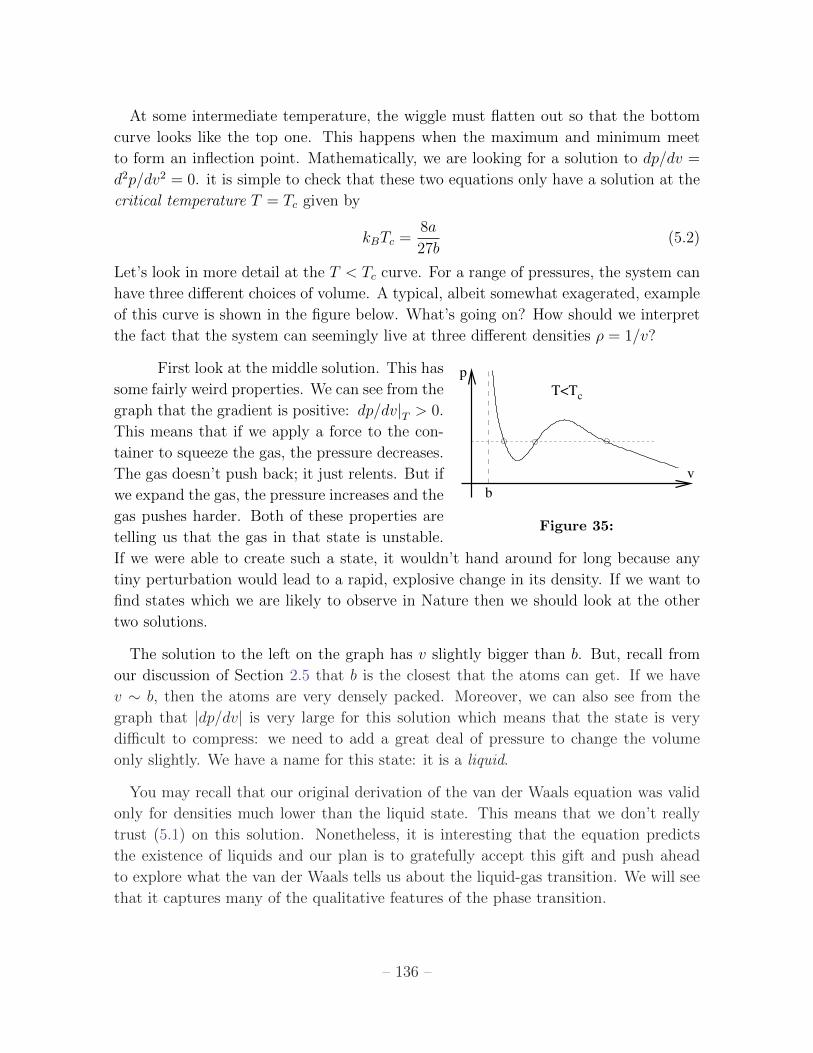
At some intermediate temperature, the wiggle must flatten out so that the bottom
curve looks like the top one. This happens when the maximum and minimum meet
to form an inflection point. Mathematically, we are looking for a solution to dp/dv =
d2p/dv2 = 0. it is simple to check that these two equations only have a solution at the
critical temperature T = Tc given by
kBTc =8a
27b(5.2)
Let’s look in more detail at the T < Tc curve. For a range of pressures, the system can
have three different choices of volume. A typical, albeit somewhat exagerated, example
of this curve is shown in the figure below. What’s going on? How should we interpret
the fact that the system can seemingly live at three different densities ρ = 1/v?
First look at the middle solution. This has
b
p
T<Tc
v
Figure 35:
some fairly weird properties. We can see from the
graph that the gradient is positive: dp/dv|T > 0.
This means that if we apply a force to the con-
tainer to squeeze the gas, the pressure decreases.
The gas doesn’t push back; it just relents. But if
we expand the gas, the pressure increases and the
gas pushes harder. Both of these properties are
telling us that the gas in that state is unstable.
If we were able to create such a state, it wouldn’t hand around for long because any
tiny perturbation would lead to a rapid, explosive change in its density. If we want to
find states which we are likely to observe in Nature then we should look at the other
two solutions.
The solution to the left on the graph has v slightly bigger than b. But, recall from
our discussion of Section 2.5 that b is the closest that the atoms can get. If we have
v ∼ b, then the atoms are very densely packed. Moreover, we can also see from the
graph that |dp/dv| is very large for this solution which means that the state is very
difficult to compress: we need to add a great deal of pressure to change the volume
only slightly. We have a name for this state: it is a liquid.
You may recall that our original derivation of the van der Waals equation was valid
only for densities much lower than the liquid state. This means that we don’t really
trust (5.1) on this solution. Nonetheless, it is interesting that the equation predicts
the existence of liquids and our plan is to gratefully accept this gift and push ahead
to explore what the van der Waals tells us about the liquid-gas transition. We will see
that it captures many of the qualitative features of the phase transition.
– 136 –

The last of the three solutions is the one on the right in the figure. This solution has
v b and small |dp/dv|. It is the gas state. Our goal is to understand what happens
in between the liquid and gas state. We know that the naive, middle, solution given to
us by the van der Waals equation is unstable. What replaces it?
5.1.1 Phase Equilibrium
Throughout our derivation of the van der Waals equation in Section 2.5, we assumed
that the system was at a fixed density. But the presence of two solutions — the liquid
and gas state — allows us to consider more general configurations: part of the system
could be a liquid and part could be a gas.
How do we figure out if this indeed happens? Just because both liquid and gas states
can exist, doesn’t mean that they can cohabit. It might be that one is preferred over
the other. We already saw some conditions that must be satisfied in order for two
systems to sit in equilibrium back in Section 1. Mechanical and thermal equilibrium
are guaranteed if two systems have the same pressure and temperature respectively.
But both of these are already guaranteed by construction for our two liquid and gas
solutions: the two solutions sit on the same isotherm and at the same value of p. We’re
left with only one further requirement that we must satisfy which arises because the
two systems can exchange particles. This is the requirement of chemical equilibrium,
µliquid = µgas (5.3)
Because of the relationship (4.22) between the chemical potential and the Gibbs free
energy, this is often expressed as
gliquid = ggas (5.4)
where g = G/N is the Gibbs free energy per particle.
Notice that all the equilibrium conditions involve only intensive quantities: p, T and
µ. This means that if we have a situation where liquid and gas are in equilibrium, then
we can have any number Nliquid of atoms in the liquid state and any number Ngas in
the gas state. But how can we make sure that chemical equilibrium (5.3) is satisfied?
Maxwell Construction
We want to solve µliquid = µgas. We will think of the chemical potential as a function of
p and T : µ = µ(p, T ). Importantly, we won’t assume that µ(p, T ) is single valued since
that would be assuming the result we’re trying to prove! Instead we will show that if
we fix T , the condition (5.3) can only be solved for a very particular value of pressure
– 137 –

p. To see this, start in the liquid state at some fixed value of p and T and travel along
the isotherm. The infinitesimal change in the chemical potential is
dµ =∂µ
∂p
∣∣∣∣T
dp
However, we can get an expression for ∂µ/∂p by recalling that arguments involving
extensive and intensive variables tell us that the chemical potential is proportional to
the Gibbs free energy: G(p, T,N) = µ(p, T )N (4.22). Looking back at the variation of
the Gibbs free energy (4.21) then tells us that
∂G
∂p
∣∣∣∣N,T
=∂µ
∂p
∣∣∣∣T
N = V (5.5)
Integrating along the isotherm then tells us the chem-
b
p
T<Tc
v
Figure 36:
ical potential of any point on the curve,
µ(p, T ) = µliquid +
∫ p
pliquid
dp′V (p′, T )
N
When we get to gas state at the same pressure p =
pliquid that we started from, the condition for equi-
librium is µ = µliquid. Which means that the integral
has to vanish. Graphically this is very simple to de-
scribe: the two shaded areas in the graph must have equal area. This condition, known
as the Maxwell construction, tells us the pressure at which gas and liquid can co-exist.
I should confess that there’s something slightly dodgy about the Maxwell construc-
tion. We already argued that the part of the isotherm with dp/dv > 0 suffers an
instability and is unphysical. But we needed to trek along that part of the curve to
derive our result. There are more rigorous arguments that give the same answer.
For each isotherm, we can determine the pressure at which the liquid and gas states
are in equilibrium. The gives us the co-existence curve, shown by the dotted line in
Figure 37. Inside this region, liquid and gas can both exist at the same temperature
and pressure. But there is nothing that tells us how much gas there should be and how
much liquid: atoms can happily move from the liquid state to the gas state. This means
that while the density of gas and liquid is fixed, the average density of the system is
not. It can vary between the gas density and the liquid density simply by changing the
amount of liquid. The upshot of this argument is that inside the co-existence curves,
the isotherms simply become flat lines, reflecting the fact that the density can take any
value. This is shown in graph on the right of Figure 37.
– 138 –

p
v
cT=T
p
v
cT=T
Figure 37: The co-existence curve in red, resulting in constant pressure regions consisting
of a harmonious mixture of vapour and liquid.
To illustrate the physics of this situation, suppose that we sit
Figure 38:
at some fixed density ρ = 1/v and cool the system down from a
high temperature to T < Tc at a point inside the co-existence curve
so that we’re now sitting on one of the flat lines. Here, the system
is neither entirely liquid, nor entirely gas. Instead it will split into
gas, with density 1/vgas, and liquid, with density 1/vliquid so that the
average density remains 1/v. The system undergoes phase separation.
The minimum energy configuration will typically be a single phase of
liquid and one of gas because the interface between the two costs energy. (We will derive
an expression for this energy in Section 5.5). The end result is shown on the right. In
the presence of gravity, the higher density liquid will indeed sink to the bottom.
Meta-Stable States
We’ve understood what replaces the unstable region
v
p
Figure 39:
of the van der Waals phase diagram. But we seem to have
removed more states than anticipated: parts of the Van
der Waals isotherm that had dp/dv < 0 are contained in
the co-existence region and replaced by the flat pressure
lines. This is the region of the p-V phase diagram that
is contained between the two dotted lines in the figure to
the right. The outer dotted line is the co-existence curve.
The inner dotted curve is constructed to pass through the
stationary points of the van der Waals isotherms. It is
called the spinodial curve.
– 139 –

The van der Waals states which lie between the spinodial curve and the co-existence
curve are good states. But they are meta-stable. One can show that their Gibbs free
energy is higher than that of the liquid-gas equilibrium at the same p and T . However,
if we compress the gas very slowly we can coax the system into this state. It is known
as a supercooled vapour. It is delicate. Any small disturbance will cause some amount
of the gas to condense into the liquid. Similarly, expanding a liquid beyond the co-
existence curve results in an meta-stable, superheated liquid.
5.1.2 The Clausius-Clapeyron Equation
We can also choose to plot the liquid-gas phase dia-
Tc
liquid
gas
critical pointp
T
Figure 40:
gram on the p− T plane. Here the co-existence region is
squeezed into a line: if we’re sitting in the gas phase and
increase the pressure just a little bit at at fixed T < Tcthen we jump immediately to the liquid phase. This ap-
pears as a discontinuity in the volume. Such discontinu-
ities are the sign of a phase transition. The end result
is sketched in the figure to the right; the thick solid line
denotes the presence of a phase transition.
Either side of the line, all particles are either in the gas or liquid phase. We know
from (5.4) that the Gibbs free energies (per particle) of these two states are equal,
gliquid = ggas
So G is continuous as we move across the line of phase transitions. Suppose that we
sit on the line itself and move along it. How does g change? We can easily compute
this from (4.21),
dGliquid = −SliquiddT + Vliquiddp ⇒ dgliquid = −sliquiddT + vliquiddp
where, just as g = G/N an v = V/N , the entropy density is s = S/N . Equating this
with the free energy in the gaseous phase gives
dgliquid = −sliquiddT + vliquiddp = dggas = −sgasdT + vgasdp
This can be rearranged to gives us a nice expression for the slope of the line of phase
transitions in the p− T plane. It is
dp
dT=sgas − sliquid
vgas − vliquid
– 140 –

We usually define the specific latent heat
L = T (sgas − sliquid)
This is the energy released per particle as we pass through the phase transition. We
see that the slope of the line in the p−T plane is determined by the ratio of latent heat
released in the phase transition and the discontinuity in volume. The result is known
as the Clausius-Clapeyron equation,
dp
dT=
L
T (vgas − vliquid)(5.6)
There is a classification of phase transitions, due originally to Ehrenfest. When the
nth derivative of a thermodynamic potential (either F or G usually) is discontinuous,
we say we have an nth order phase transition. In practice, we nearly always deal with
first, second and (very rarely) third order transitions. The liquid-gas transition releases
latent heat, which means that S = −∂F/∂T is discontinuous. Alternatively, we can
say that V = ∂G/∂p is discontinuous. Either way, it is a first order phase transition.
The Clausius-Clapeyron equation (5.6) applies to any first order transition.
As we approach T → Tc, the discontinuity dimin- p
T
Tc
solid
gas
liquid
Figure 41:
ishes and Sliquid → Sgas. At the critical point T = Tc we
have a second order phase transition. Above the critical
point, there is no sharp distinction between the gas phase
and liquid phase.
For most simple materials, the phase diagram above is
part of a larger phase diagram which includes solids at
smaller temperatures or higher pressures. A generic ver-
sion of such a phase diagram is shown to the right. The
van der Waals equation is missing the physics of solidifica-
tion and includes only the liquid-gas line.
An Approximate Solution to the Clausius-Clapeyron Equation
We can solve the Clausius-Clapeyron solution if we make the following assumptions:
• The latent heat L is constant.
• vgas vliquid, so vgas − vliquid ≈ vgas. For water, this is an error of less than 0.1%
• Although we derived the phase transition using the van der Waals equation, now
we’ve got equation (5.6) we’ll pretend the gas obeys the ideal gas law pv = kBT .
– 141 –

With these assumptions, it is simple to solve (5.6). It reduces to
dp
dT=
Lp
kBT 2⇒ p = p0e
−L/kBT
5.1.3 The Critical Point
Let’s now return to discuss some aspects of life at the critical point. We previously
worked out the critical temperature (5.2) by looking for solutions to simultaneous equa-
tions ∂p/∂v = ∂2p/∂v2 = 0. There’s a slightly more elegant way to find the critical
point which also quickly gives us pc and vc as well. We rearrange the van der Waals
equation (5.1) to get a cubic,
pv3 − (pb+ kBT )v2 + av − ab = 0
For T < Tc, this equation has three real roots. For T > Tc there is just one. Precisely at
T = Tc, the three roots must therefore coincide (before two move off onto the complex
plane). At the critical point, this curve can be written as
pc(v − vc)3 = 0
Comparing the coefficients tells us the values at the critical point,
kBTc =8a
27b, vc = 3b , pc =
a
27b2(5.7)
The Law of Corresponding States
We can invert the relations (5.7) to express the parameters a and b in terms of the
critical values, which we then substitute back into the van der Waals equation. To this
end, we define the reduced variables,
T =T
Tc, v =
v
vcp =
p
pc
The advantage of working with T , v and p is that it allows us to write the van der
Waals equation (5.1) in a form that is universal to all gases, usually referred to as the
law of corresponding states
p =8
3
T
v − 1/3− 3
v2
Moreover, because the three variables Tc, pc and vc at the critical point are expressed
in terms of just two variables, a and b (5.7), we can construct a combination of them
– 142 –

Figure 42: The co-existence curve for gases. Data is plotted for Ne, Ar, Kr,Xe, N2, O2, CO
and CH4.
which is independent of a and b and therefore supposedly the same for all gases. This
is the universal compressibility ratio,
pcvckBTc
=3
8= 0.375 (5.8)
Comparing to real gases, this number is a little high. Values range from around
0.28 to 0.3. We shouldn’t be too discouraged by this; after all, we knew from the
beginning that the van der Waals equation is unlikely to be accurate in the liquid
regime. Moreover, the fact that gases have a critical point (defined by three variables
Tc, pc and vc) guarantees that a similar relationship would hold for any equation of
state which includes just two parameters (such as a and b) but would most likely fail
to hold for equations of state that included more than two parameters.
Dubious as its theoretical foundation is, the law of corresponding states is the first
suggestion that something remarkable happens if we describe a gas in terms of its
reduced variables. More importantly, there is striking experimental evidence to back
this up! Figure 42 shows the Guggenheim plot, constructed in 1945. The co-existence
curve for 8 different gases in plotted in reduced variables: T along the vertical axis;
ρ = 1/v along the horizontal. The gases vary in complexity from the simple monatomic
gas Ne to the molecule CH4. As you can see, the co-existence curve for all gases is
essentially the same, with the chemical make-up largely forgotten. There is clearly
something interesting going on. How to understand it?
Critical Exponents
We will focus attention on physics close to the critical point. It is not immediately
– 143 –

obvious what are the right questions to ask. It turns out that the questions which
have the most interesting answer are concerned with how various quantities change as
we approach the critical point. There are lots of ways to ask questions of this type
since there are many quantities of interest and, for each of them, we could approach
the critical point from different directions. Here we’ll look at the behaviour of three
quantities to get a feel for what happens.
First, we can ask what happens to the difference in (inverse) densities vgas− vliquid as
we approach the critical point along the co-existence curve. For T < Tc, or equivalently
T < 1, the reduced van der Waals equation (5.8) has two stable solutions,
p =8T
3vliquid − 1− 3
v2liquid
=8T
3vgas − 1− 3
v2gas
If we solve this for T , we have
T =(3vliquid − 1)(3vgas − 1)(vliquid + vgas)
8v2gasv
2liquid
Notice that as we approach the critical point, vgas, vliquid → 1 and the equation above
tells us that T → 1 as expected. We can see exactly how we approach T = 1 by
expanding the right right-hand side for small ε ≡ vgas − vliquid. To do this quickly, it’s
best to notice that the equation is symmetric in vgas and vliquid, so close to the critical
point we can write vgas = 1 + ε/2 and vliquid = 1 − ε/2. Substituting this into the
equation above and keeping just the leading order term, we find
T ≈ 1− 1
16(vgas − vliquid)2
Or, re-arranging, as we approach Tc along the co-existence curve,
vgas − vliquid ∼ (Tc − T )1/2 (5.9)
This is the answer to our first question.
Our second variant of the question is: how does the volume change with pressure
as we move along the critical isotherm. It turns out that we can answer this question
without doing any work. Notice that at T = Tc, there is a unique pressure for a given
volume p(v, Tc). But we know that ∂p/∂v = ∂2p/∂v2 = 0 at the critical point. So a
Taylor expansion around the critical point must start with the cubic term,
p− pc ∼ (v − vc)3 (5.10)
This is the answer to our second question.
– 144 –

Our third and final variant of the question concerns the compressibility, defined as
κ = −1
v
∂v
∂p
∣∣∣∣T
(5.11)
We want to understand how κ changes as we approach T → Tc from above. In fact, we
met the compressibility before: it was the feature that first made us nervous about the
van der Waals equation since κ is negative in the unstable region. We already know
that at the critical point ∂p/∂v|Tc = 0. So expanding for temperatures close to Tc, we
expect
∂p
∂v
∣∣∣∣T ;v=vc
= −a(T − Tc) + . . .
This tells us that the compressibility should diverge at the critical point, scaling as
κ ∼ (T − Tc)−1 (5.12)
We now have three answers to three questions: (5.9), (5.10) and (5.12). Are they
right?! By which I mean: do they agree with experiment? Remember that we’re not
sure that we can trust the van der Waals equation at the critical point so we should be
nervous. However, there is also reason for some confidence. Notice, in particular, that
in order to compute (5.10) and (5.12), we didn’t actually need any details of the van
der Waals equation. We simply needed to assume the existence of the critical point
and an analytic Taylor expansion of various quantities in the neighbourhood. Given
that the answers follow from such general grounds, one may hope that they provide
the correct answers for a gas in the neighbourhood of the critical point even though we
know that the approximations that went into the van der Waals equation aren’t valid
there. Fortunately, that isn’t the case: physics is much more interesting than that!
The experimental results for a gas in the neighbourhood of the critical point do share
one feature in common with the discussion above: they are completely independent of
the atomic make-up of the gas. However, the scaling that we computed using the van
der Waals equation is not fully accurate. The correct results are as follows. As we
approach the critical point along the co-existence curve, the densities scale as
vgas − vliquid ∼ (Tc − T )β with β ≈ 0.32
(Note that the exponent β has nothing to do with inverse temperature. We’re just near
the end of the course and running out of letters and β is the canonical name for this
exponent). As we approach along an isotherm,
p− pc ∼ (v − vc)δ with δ ≈ 4.8
– 145 –

Finally, as we approach Tc from above, the compressibility scales as
κ ∼ (T − Tc)−γ with γ ≈ 1.2
The quantities β, γ and δ are examples of critical exponents. We will see more of them
shortly. The van der Waals equation provides only a crude first approximation to the
critical exponents.
Fluctuations
We see that the van der Waals equation didn’t do too badly in capturing the dynamics
of an interacting gas. It gets the qualitative behaviour right, but fails on precise
quantitative tests. So what went wrong? We mentioned during the derivation of the
van der Waals equation that we made certain approximations that are valid only at
low density. So perhaps it is not surprising that it fails to get the numbers right near
the critical point v = 3b. But there’s actually a deeper reason that the van der Waals
equation fails: fluctuations.
This is simplest to see in the grand canonical ensemble. Recall that back in Section
1 that we argued that ∆N/N ∼ 1/√N , which allowed us to happily work in the
grand canonical ensemble even when we actually had fixed particle number. In the
context of the liquid-gas transition, fluctuating particle number is the same thing as
fluctuating density ρ = N/V . Let’s revisit the calculation of ∆N near the critical
point. Using (1.45) and (1.48), the grand canonical partition function can be written
as logZ = βV p(T, µ), so the average particle number (1.42) is
〈N〉 = V∂p
∂µ
∣∣∣∣T,V
We already have an expression for the variance in the particle number in (1.43),
∆N2 =1
β
∂〈N〉∂µ
∣∣∣∣T,V
Dividing these two expressions, we have
∆N2
N=
1
V β
∂〈N〉∂µ
∣∣∣∣T,V
∂µ
∂p
∣∣∣∣T,V
=1
V β
∂〈N〉∂p
∣∣∣∣T,V
But we can re-write this expression using the general relationship between partial
derivatives ∂x/∂y|z ∂y/∂z|x ∂z/∂x|y = −1. We then have
∆N2
N= − 1
β
∂〈N〉∂V
∣∣∣∣p,T
1
V
∂V
∂p
∣∣∣∣N,T
– 146 –

This final expression relates the fluctuations in the particle number to the compress-
ibility (5.11). But the compressibility is diverging at the critical point and this means
that there are large fluctuations in the density of the fluid at this point. The result is
that any simple equation of state, like the van der Waals equation, which works only
with the average volume, pressure and density will miss this key aspect of the physics.
Understanding how to correctly account for these fluctuations is the subject of critical
phenomena. It has close links with the renormalization group and conformal field theory
which also arise in particle physics and string theory. You will meet some of these ideas
in next year’s Statistical Field Theory course. Here we will turn to a different phase
transition which will allow us to highlight some of the key ideas.
5.2 The Ising Model
The Ising model is one of the touchstones of modern physics; a simple system that
exhibits non-trivial and interesting behaviour.
The Ising model consists of N sites in a d-dimensional lattice. On each lattice site
lives a quantum spin that can sit in one of two states: spin up or spin down. We’ll call
the eigenvalue of the spin on the ith lattice site si. If the spin is up, si = +1; if the spin
is down, si = −1.
The spins sit in a magnetic field that endows an energy advantage to those which
point up,
EB = −BN∑i=1
si
(A comment on notation: B should be properly denoted H. We’re sticking with B to
avoid confusion with the Hamiltonian. There is also a factor of the magnetic moment
which has been absorbed into the definition of B). The lattice system with energy EBis equivalent to the two-state system that we first met when learning the techniques of
statistical mechanics back in Section 1.2.3. However, the Ising model contains an addi-
tional complication that makes the sysem much more interesting: this is an interaction
between neighbouring spins. The full energy of the system is therefore,
E = −J∑〈ij〉
sisj −B∑i
si (5.13)
The notation 〈ij〉 means that we sum over all “nearest neighbour” pairs in the lattice.
The number of such pairs depends both on the dimension d and the type of lattice.
– 147 –

We’ll denote the number of nearest neighbours as q. For example, in d = 1 a lattice
has q = 2; in d = 2, a square lattice has q = 4. A square lattice in d dimensions has
q = 2d.
If J > 0, neighbouring spins prefer to be aligned (↑↑ or ↓↓). In the context of
magnetism, such a system is called a ferromagnet. If J < 0, the spins want to anti-
align (↑↓). This is an anti-ferromagnet. In the following, we’ll choose J > 0 although
for the level of discussion needed for this course, the differences are minor.
We work in the canonical ensemble and introduce the partition function
Z =∑si
e−βE[si] (5.14)
While the effect of both J > 0 and B 6= 0 is to make it energetically preferable for the
spins to align, the effect of temperature will be to randomize the spins, with entropy
winnning out over energy. Our interest is in the average spin, or average magnetization
m =1
N
∑i
〈si〉 =1
Nβ
∂logZ
∂B(5.15)
The Ising Model as a Lattice Gas
Before we develop techniques to compute the partition function (5.14), it’s worth point-
ing out that we can drape slightly different words around the mathematics of the Ising
model. It need not be interpreted as a system of spins; it can also be thought of as a
lattice description of a gas.
To see this, consider the same d-dimensional lattice as before, but now with particles
hopping between lattice sites. These particles have hard cores, so no more than one
can sit on a single lattice site. We introduce the variable ni ∈ 0, 1 to specify whether
a given lattice site, labelled by i, is empty (ni = 0) or filled (ni = 1). We can also
introduce an attractive force between atoms by offering them an energetic reward if
they sit on neighbouring sites. The Hamiltonian of such a lattice gas is given by
E = −4J∑〈ij〉
ninj − µ∑i
ni
where µ is the chemical potential which determines the overall particle number. But this
Hamiltonian is trivially the same as the Ising model (5.13) if we make the identification
si = 2ni − 1 ∈ −1, 1
The chemical potenial µ in the lattice gas plays the role of magnetic field in the spin
system while the magnetization of the system (5.15) measures the average density of
particles away from half-filling.
– 148 –

5.2.1 Mean Field Theory
For general lattices, in arbitrary dimension d, the sum (5.14) cannot be performed. An
exact solution exists in d = 1 and, when B = 0, in d = 2. (The d = 2 solution is
originally due to Onsager and is famously complicated! Simpler solutions using more
modern techniques have since been discovered).
Here we’ll develop an approximate method to evaluate Z known as mean field theory.
We write the interactions between neighbouring spins in term of their deviation from
the average spin m,
sisj = [(si −m) +m][(sj −m) +m]
= (si −m)(sj −m) +m(sj −m) +m(si −m) +m2
The mean field approximation means that we assume that the fluctuations of spins away
from the average are small which allows us to neglect the first term above. Notice that
this isn’t the statement that the variance of an individual spin is small; that can never
be true because si takes values +1 or −1 so 〈s2i 〉 = 1 and the variance 〈(si −m)2〉 is
always large. Instead, the mean field approximation is a statement about fluctuations
between spins on neighbouring sites, so the first term above can be neglected when
summing over∑〈ij〉. We can then write the energy (5.13) as
Emf = −J∑〈ij〉
[m(si + sj)−m2]−B∑i
si
=1
2JNqm2 − (Jqm+B)
∑i
si (5.16)
where the factor of Nq/2 in the first term is simply the number of nearest neighbour
pairs∑〈ij〉. The factor or 1/2 is there because
∑〈ij〉 is a sum over pairs rather than a
sum of individual sites. (If you’re worried about this formula, you should check it for
a simple square lattice in d = 1 and d = 2 dimensions). A similar factor in the second
term cancelled the factor of 2 due to (si + sj).
We see that the mean field approximation has removed the interactions. The Ising
model reduces to the two state system that we saw way back in Section 1. The result
of the interactions is that a given spin feels the average effect of its neighbour’s spins
through a contribution to the effective magnetic field,
Beff = B + Jqm
Once we’ve taken into account this extra contribution to Beff , each spin acts indepen-
– 149 –

tanh
m
m0
−m
tanh
m
0
Figure 43: tanh(Jqmβ) for Jqβ < 1 Figure 44: tanh(Jqmβ) for Jqβ > 1
dently and it is easy to write the partition function. It is
Z = e−12βJNqm2 (
e−βBeff + eβBeff)N
= e−12βJNqm2
2N coshN βBeff (5.17)
However, we’re not quite done. Our result for the partition function Z depends on Beff
which depends on m which we don’t yet know. However, we can use our expression for
Z to self-consistently determine the magnetization (5.15). We find,
m = tanh(βB + βJqm) (5.18)
We can now solve this equation to find the magnetization for various values of T and B:
m = m(T,B). It is simple to see the nature of the solutions using graphical methods.
B=0
Let’s first consider the situation with vanishing magnetic field, B = 0. The figures
above show the graph linear in m compared with the tanh function. Since tanhx ≈x− 1
3x3+. . ., the slope of the graph near the origin is given by βJq. This then determines
the nature of the solution.
• The first graph depicts the situation for βJq < 1. The only solution is m = 0.
This means that at high temperatures kBT > Jq, there is no average magne-
tization of the system. The entropy associated to the random temperature flu-
cutations wins over the energetically preferred ordered state in which the spins
align.
• The second graph depicts the situation for βJq > 1. Now there are three solu-
tions: m = ±m0 and m = 0. It will turn out that the middle solution, m = 0, is
unstable. (This solution is entirely analogous to the unstable solution of the van
der Waals equation. We will see this below when we compute the free energy).
– 150 –

For the other two possible solutions, m = ±m0, the magnetization is non-zero.
Here we see the effects of the interactions begin to win over temperature. Notice
that in the limit of vanishing temperature, β →∞, m0 → 1. This means that all
the spins are pointing in the same direction (either up or down) as expected.
• The critical temperature separating these two cases is
kBTc = Jq (5.19)
The results described above are perhaps rather surprising. Based on the intuition that
things in physics always happen smoothly, one might have thought that the magneti-
zation would drop slowly to zero as T → ∞. But that doesn’t happen. Instead the
magnetization turns off abruptly at some finite value of the temperature T = Tc, with
no magnetization at all for higher temperatures. This is the characteristic behaviour
of a phase transition.
B 6= 0
For B 6= 0, we can solve the consistency equation (5.18) in a similar fashion. There are
a couple of key differences to the B 6= 0 case. Firstly, there is now no phase transition
at fixed B as we vary temperature T . Instead, for very large temperatures kBT Jq,
the magnetization goes smoothly to zero as
m→ B
kBTas T →∞
At low temperatures, the magnetization again asymptotes to the state m→ ±1 which
minimizes the energy. Except this time, there is no ambiguity as to whether the system
chooses m = +1 or m = −1. This is entirely determined by the sign of the magnetic
field B.
In fact the low temperature behaviour requires slightly more explanation. For small
values of B and T , there are again three solutions to (5.18). This follows simply from
continuity: there are three solutions for T < Tc and B = 0 shown in Figure 44 and these
must survive in some neighbourhood of B = 0. One of these solutions is again unstable.
However, of the remaining two only one is now stable: that with sign(m) = sign(B).
The other is meta-stable. We will see why this is the case shortly when we come to
discuss the free energy.
– 151 –

T
m
+1
−1
m
T
B<0
B>0+1
−1
Figure 45: Magnetization with B = 0
and the phase transtion
Figure 46: Magnetization at B 6= 0.
The net result of our discussion is depicted in the figures above. When B = 0
there is a phase transition at T = Tc. For T < Tc, the system can sit in one of two
magnetized states with m = ±m0. In contrast, for B 6= 0, there is no phase transition
as we vary temperature and the system has at all times a preferred magnetization
whose sign is determined by that of B. Notice however, we do have a phase transition
if we fix temperature at T < Tc and vary B from negative to positive. Then the
magnetization jumps discontinuously from a negative value to a positive value. Since
the magnetization is a first derivative of the free energy (5.15), this is a first order
phase transition. In contrast, moving along the temperature axis at B = 0 results in a
second order phase transition at T = Tc.
5.2.2 Critical Exponents
It is interesting to compare the phase transition of the Ising model with that of the
liquid-gas phase transition. The two are sketched in the Figure 47 above. In both cases,
we have a first order phase transition and a quantity jumps discontinuously at T < Tc.
In the case of the liquid-gas, it is the density ρ = 1/v that jumps as we vary pressure;
in the case of the Ising model it is the magnetization m that jumps as we vary the
magnetic field. Moreover, in both cases the discontinuity disappears as we approach
T = Tc.
We can calculate critical exponents for the Ising model. To compare with our discus-
sion for the liquid-gas critical point, we will compute three quantities. First, consider
the magnetization at B = 0. We can ask how this magnetization decreases as we tend
towards the critical point. Just below T = Tc, m is small and we can Taylor expand
(5.18) to get
m ≈ βJqm− 1
3(βJqm)3 + . . .
– 152 –

T
p
Tc Tc
liquid
gas
critical point
T
B
critical point
Figure 47: A comparison of the phase diagram for the liquid-gas system and the Ising model.
The magnetization therefore scales as
m0 ∼ ±(Tc − T )1/2 (5.20)
This is to be compared with the analogous result (5.9) from the van der Waals equation.
We see that the values of the exponents are the same in both cases. Notice that the
derivative dm/dT becomes infinite as we approach the critical point. In fact, we had
already anticipated this when we drew the plot of the magnetization in Figure 45.
Secondly, we can sit at T = Tc and ask how the magnetization changes as we approach
B = 0. We can read this off from (5.18). At T = Tc we have βJq = 1 and the
consistency condition becomes m = tanh(B/Jq +m). Expanding for small B gives
m ≈ B
Jq+m− 1
3
(B
Jq+m
)3
+ . . . ≈ B
Jq+m− 1
3m3 +O(B2)
So we find that the magnetization scales as
m ∼ B1/3 (5.21)
Notice that this power of 1/3 is again familiar from the liquid-gas transition (5.10)
where the van der Waals equation gave vgas − vliquid ∼ (p− pc)1/3.
Finally, we can look at the magnetic susceptibility χ, defined as
χ = N∂m
∂B
∣∣∣∣T
This is analogous to the compressibility κ of the gas. We will ask how χ changes as we
approach T → Tc from above at B = 0. We differentiate (5.18) with respect to B to
get
χ =Nβ
cosh2 βJqm
(1 +
Jq
Nχ
)
– 153 –

We now evaluate this at B = 0. Since we want to approach T → Tc from above, we can
also set m = 0 in the above expression. Evaluating this at B = 0 gives us the scaling
χ =Nβ
1− Jqβ∼ (T − Tc)−1 (5.22)
Once again, we see that same critical exponent that the van der Waals equation gave
us for the gas (5.12).
5.2.3 Validity of Mean Field Theory
The phase diagram and critical exponents above were all derived using the mean field
approximation. But this was an unjustified approximation. Just as for the van der
Waals equation, we can ask the all-important question: are our results right?
There is actually a version of the Ising model for which the mean field theory is
exact: it is the d = ∞ dimensional lattice. This is unphysical (even for a string
theorist). Roughly speaking, mean field theory works for large d because each spin has
a large number of neighbours and so indeed sees something close to the average spin.
But what about dimensions of interest? Mean field theory gets things most dramati-
cally wrong in d = 1. In that case, no phase transition occurs. We will derive this result
below where we briefly describe the exact solution to the d = 1 Ising model. There is
a general lesson here: in low dimensions, both thermal and quantum fluctuations are
more important and invariably stop systems forming ordered phases.
In higher dimensions, d ≥ 2, the crude features of the phase diagram, including
the existence of a phase transition, given by mean field theory are essentially correct.
In fact, the very existence of a phase transition is already worthy of comment. The
defining feature of a phase transition is behaviour that jumps discontinuously as we
vary β or B. Mathematically, the functions must be non-analytic. Yet all properties of
the theory can be extracted from the partition function Z which is a sum of smooth,
analytic functions (5.14). How can we get a phase transition? The loophole is that Z
is only necessarily analytic if the sum is finite. But there is no such guarantee when
the number of lattice sites N → ∞. We reach a similar conclusion to that of Bose-
Einstein condensation: phase transitions only strictly happen in the thermodynamic
limit. There are no phase transitions in finite systems.
What about the critical exponents that we computed in (5.20), (5.21) and (5.22)? It
turns out that these are correct for the Ising model defined in d ≥ 4. (We will briefly
sketch why this is true at the end of this Chapter). But for d = 2 and d = 3, the
critical exponents predicted by mean field theory are only first approximations to the
true answers.
– 154 –

For d = 2, the exact solution (which goes quite substantially past this course) gives
the critical exponents to be,
m0 ∼ (Tc − T )β with β =1
8m ∼ B1/δ with δ = 15
χ ∼ (T − Tc)−γ with γ =7
4
The biggest surprise is in d = 3 dimensions. Here the critical exponents are not known
exactly. However, there has been a great deal of numerical work to determine them.
They are given by
β ≈ 0.32 , δ ≈ 4.8 , γ ≈ 1.2
But these are exactly the same critical exponents that are seen in the liquid-gas phase
transition. That’s remarkable! We saw above that the mean field approach to the Ising
model gave the same critical exponents as the van der Waals equation. But they are
both wrong. And they are both wrong in the same, complicated, way! Why on earth
would a system of spins on a lattice have anything to do with the phase transition
between a liquid and gas? It is as if all memory of the microscopic physics — the type
of particles, the nature of the interactions — has been lost at the critical point. And
that’s exactly what happens.
What we’re seeing here is evidence for universality. There is a single theory which
describes the physics at the critical point of the liquid gas transition, the 3d Ising model
and many other systems. This is a theoretical physicist’s dream! We spend a great
deal of time trying to throw away the messy details of a system to focus on the elegant
essentials. But, at a critical point, Nature does this for us! Although critical points
in two dimensions are well understood, there is still much that we don’t know about
critical points in three dimensions. This, however, is a story that will have to wait for
another day.
5.3 Some Exact Results for the Ising Model
This subsection is something of a diversion from our main interest. In later subsec-
tions, we will develop the idea of mean field theory. But first we pause to describe
some exact results for the Ising model using techniques that do not rely on the mean
field approximation. Many of the results that we derive have broader implications for
systems beyond the Ising model.
– 155 –

As we mentioned above, there is an exact solution for the Ising model in d = 1
dimension and, when B = 0, in d = 2 dimensions. Here we will describe the d = 1
solution but not the full d = 2 solution. We will, however, derive a number of results
for the d = 2 Ising model which, while falling short of the full solution, nonetheless
provide important insights into the physics.
5.3.1 The Ising Model in d = 1 Dimensions
We start with the Ising chain, the Ising model on a one dimensional line. Here we will
see that the mean field approximation fails miserably, giving qualitatively incorrect
results: the exact results shows that there are no phase transitions in the Ising chain.
The energy of the system (5.13) can be trivially rewritten as
E = −JN∑i=1
sisi+1 −B
2
N∑i=1
(si + si+1)
We will impose periodic boundary conditions, so the spins live on a circular lattice with
sN+1 ≡ s1. The partition function is then
Z =∑s1=±1
. . .∑sN=±1
N∏i=1
exp
(βJsisi+1 +
βB
2(si + si+1)
)(5.23)
The crucial observation that allows us to solve the problem is that this partition function
can be written as a product of matrices. We adopt notation from quantum mechanics
and define the 2× 2 matrix,
〈si|T |si+1〉 ≡ exp
(βJsisi+1 +
βB
2(si + si+1)
)(5.24)
The row of the matrix is specified by the value of si = ±1 and the column by si+1 = ±1.
T is known as the transfer matrix and, in more conventional notation, is given by
T =
(eβJ+βB e−βJ
e−βJ eβJ−βB
)
The sums over the spins∑
siand product over lattice sites
∏i in (5.23) simply tell us
to multiply the matrices defined in (5.24) and the partition function becomes
Z = Tr (〈s1|T |s2〉〈s2|T |s3〉 . . . 〈sN |T |s1〉) = TrTN (5.25)
– 156 –

where the trace arises because we have imposed periodic boundary conditions. To com-
plete the story, we need only compute the eigenvalues of T to determine the partition
function. A quick calculation shows that the two eigenvalues of T are
λ± = eβJ cosh βB ±√e2βJ cosh2 βB − 2 sinh 2βJ (5.26)
where, clearly, λ− < λ+. The partition function is then
Z = λN+ + λN− = λN+
(1 +
λN−λN+
)≈ λN+ (5.27)
where, in the last step, we’ve used the simple fact that if λ+ is the largest eigenvalue
then λN−/λN+ ≈ 0 for very large N .
The partition function Z contains many quantities of interest. In particular, we can
use it to compute the magnetisation as a function of temperature when B = 0. This,
recall, is the quantity which is predicted to undergo a phase transition in the mean
field approximation, going abruptly to zero at some critical temperature. In the d = 1
Ising model, the magnetisation is given by
m =1
Nβ
∂ logZ
∂B
∣∣∣∣B=0
=1
λ+β
∂λ+
∂B
∣∣∣∣B=0
= 0
We see that the true physics for d = 1 is very different than that suggested by the
mean field approximation. When B = 0, there is no magnetisation! While the J term
in the energy encourages the spins to align, this is completely overwhelmed by thermal
fluctuations for any value of the temperature.
There is a general lesson in this calculation: thermal fluctuations always win in one
dimensional systems. They never exhibit ordered phases and, for this reason, never
exhibit phase transitions. The mean field approximation is bad in one dimension.
5.3.2 2d Ising Model: Low Temperatures and Peierls Droplets
Let’s now turn to the Ising model in d = 2 dimensions. We’ll work on a square lattice
and set B = 0. Rather than trying to solve the model exactly, we’ll have more modest
goals. We will compute the partition function in two different limits: high temperature
and low temperature. We start here with the low temperature expansion.
The partition function is given by the sum over all states, weighted by e−βE. At low
temperatures, this is always dominated by the lowest lying states. For the Ising model,
– 157 –

we have
Z =∑si
exp
βJ∑〈ij〉
sisj
The low temperature limit is βJ → ∞, where the partition function can be approxi-
mated by the sum over the first few lowest energy states. All we need to do is list these
states.
The ground states are easy. There are two of them: spins all up or spins all down.
For example, the ground state with spins all up looks like
Each of these ground states has energy E = E0 = −2NJ .
The first excited states arise by flipping a single spin. Each spin has q = 4 nearest
neighbours – denoted by red lines in the example below – each of which leads to an
energy cost of 2J . The energy of each first excited state is therefore E1 = E0 + 8J .
There are, of course, N different spins that we we can flip and, correspondingly, the
first energy level has a degeneracy of N .
To proceed, we introduce a diagrammatic method to list the different states. We
draw only the “broken” bonds which connect two spins with opposite orientation and,
as in the diagram above, denote these by red lines. We further draw the flipped spins
as red dots, the unflipped spins as blue dots. The energy of the state is determined
simply by the number of red lines in the diagram. Pictorially, we write the first excited
state as
E1 = E0 + 8J
Degeneracy = N
– 158 –

The next lowest state has six broken bonds. It takes the form
E2 = E0 + 12J
Degeneracy = 2N
where the extra factor of 2 in the degeneracy comes from the two possible orientations
(vertical and horizontal) of the graph.
Things are more interesting for the states which sit at the third excited level. These
have 8 broken bonds. The simplest configuration consists of two, disconnected, flipped
spins
E3 = E0 + 16J
Degeneracy = 12N(N − 5)
(5.28)
The factor of N in the degeneracy comes from placing the first graph; the factor of
N − 5 arises because the flipped spin in the second graph can sit anywhere apart from
on the five vertices used in the first graph. Finally, the factor of 1/2 arises from the
interchange of the two graphs.
There are also three further graphs with the same energy E3. These are
E3 = E0 + 16J
Degeneracy = N
and
E3 = E0 + 16J
Degeneracy = 2N
– 159 –

where the degeneracy comes from the two orientations (vertical and horizontal). And,
finally,
E3 = E0 + 16J
Degeneracy = 4N
where the degeneracy comes from the four orientations (rotating the graph by 90).
Adding all the graphs above together gives us an expansion of the partition function
in power of e−βJ 1. This is
Z = 2e2NβJ
(1 +Ne−8βJ + 2Ne−12βJ +
1
2(N2 + 9N)e−16βJ + . . .
)(5.29)
where the overall factor of 2 originates from the two ground states of the system.
We’ll make use of the specific coefficients in this expansion in Section 5.3.4. Before
we focus on the physics hiding in the low temperature expansion, it’s worth making a
quick comment that something quite nice happens if we take the log of the partition
function,
logZ = log 2 + 2NβJ +Ne−8βJ + 2Ne−12βJ +9
2Ne−16βJ + . . .
The thing to notice is that the N2 term in the partition function (5.29) has cancelled
out and logZ is proportional to N , which is to be expected since the free energy of
the system is extensive. Looking back, we see that the N2 term was associated to the
disconnected diagrams in (5.28). There is actually a general lesson hiding here: the
partition function can be written as the exponential of the sum of connected diagrams.
We saw exactly the same issue arise in the cluster expansion in (2.37).
Peierls Droplets
Continuing the low temperature expansion provides a heuristic, but physically intuitive,
explanation for why phase transitions happen in d ≥ 2 dimensions but not in d = 1.
As we flip more and more spins, the low energy states become droplets, consisting of a
region of space in which all the spins are flipped, surrounded by a larger sea in which
the spins have their original alignment. The energy cost of such a droplet is roughly
E ∼ 2JL
– 160 –

where L is the perimeter of the droplet. Notice that the energy does not scale as the
area of the droplet since all spins inside are aligned with their neighbours. It is only
those on the edge which are misaligned and this is the reason for the perimeter scaling.
To understand how these droplets contribute to the partition function, we also need to
know their degeneracy. We will now argue that the degeneracy of droplets scales as
Degeneracy ∼ eαL
for some value of α. To see this, consider firstly the problem of a random walk on a 2d
square lattice. At each step, we can move in one of four directions. So the number of
paths of length L is
#paths ∼ 4L = eL log 4
Of course, the perimeter of a droplet is more constrained that a random walk. Firstly,
the perimeter can’t go back on itself, so it really only has three directions that it can
move in at each step. Secondly, the perimeter must return to its starting point after L
steps. And, finally, the perimeter cannot self-intersect. One can show that the number
of paths that obey these conditions is
#paths ∼ eαL
where log 2 < α < log 3. Since the degeneracy scales as eαL, the entropy of the droplets
is proportional to L.
The fact that both energy and entropy scale with L means that there is an interesting
competition between them. At temperatures where the droplets are important, the
partition function is schematically of the form
Z ∼∑L
eαLe−2βJL
For large β (i.e. low temperature) the partition function converges. However, as the
temperature increases, one reaches the critical temperature
kBTc ≈2J
α(5.30)
where the partition function no longer converges. At this point, the entropy wins over
the energy cost and it is favourable to populate the system with droplets of arbitrary
sizes. This is the how one sees the phase transition in the partition function. For
temperature above Tc, the low-temperature expansion breaks down and the ordered
magnetic phase is destroyed.
– 161 –

We can also use the droplet argument to see why phase transitions don’t occur in
d = 1 dimension. On a line, the boundary of any droplet always consists of just
two points. This means that the energy cost to forming a droplet is always E = 2J ,
regardless of the size of the droplet. But, since the droplet can exist anywhere along the
line, its degeneracy is N . The net result is that the free energy associated to creating
a droplet scales as
F ∼ 2J − kBT logN
and, as N →∞, the free energy is negative for any T > 0. This means that the system
will prefer to create droplets of arbitrary length, randomizing the spins. This is the
intuitive reason why there is no magnetic ordered phase in the d = 1 Ising model.
5.3.3 2d Ising Model: High Temperatures
We now turn to the 2d Ising model in the opposite limit of high temperature. Here we
expect the partition function to be dominated by the completely random, disordered
configurations of maximum entropy. Our goal is to find a way to expand the partition
function in βJ 1.
We again work with zero magnetic field, B = 0 and write the partition function as
Z =∑si
exp
βJ∑〈ij〉
sisj
=∑si
∏〈ij〉
eβJsisj
There is a useful way to rewrite eβJsisj which relies on the fact that the product sisjonly takes ±1. It doesn’t take long to check the following identity:
eβJsisj = cosh βJ + sisj sinh βJ
= cosh βJ (1 + sisj tanh βJ)
Using this, the partition function becomes
Z =∑si
∏〈ij〉
cosh βJ (1 + sisj tanh βJ)
= (cosh βJ)qN/2∑si
∏〈ij〉
(1 + sisj tanh βJ) (5.31)
where the number of nearest neighbours is q = 4 for the 2d square lattice.
– 162 –

With the partition function in this form, there is a natural expansion which suggests
itself. At high temperatures βJ 1 which, of course, means that tanh βJ 1.
But the partition function is now naturally a product of powers of tanh βJ . This is
somewhat analogous to the cluster expansion for the interacting gas that we met in
Section 2.5.3. As in the cluster expansion, we will represent the expansion graphically.
We need no graphics for the leading order term. It has no factors of tanh βJ and is
simply
Z ≈ (cosh βJ)2N∑si
1 = 2N(cosh βJ)2N
That’s simple.
Let’s now turn to the leading correction. Expanding the partition function (5.31),
each power of tanh βJ is associated to a nearest neighbour pair 〈ij〉. We’ll represent
this by drawing a line on the lattice:
i j = sisj tanh βJ
But there’s a problem: each factor of tanh βJ in (5.31) also comes with a sum over all
spins si and sj. And these are +1 and −1 which means that they simply sum to zero,∑si,sj
sisj = +1− 1− 1 + 1 = 0
How can we avoid this? The only way is to make sure that we’re summing over an even
number of spins on each site, since then we get factors of s2i = 1 and no cancellations.
Graphically, this means that every site must have an even number of lines attached to
it. The first correction is then of the form
1 2
3 4
= (tanh βJ)4∑si
s1s2 s2s3 s3s4 s4s1 = 24(tanh βJ)4
There are N such terms since the upper left corner of the square can be on any one
of the N lattice sites. (Assuming periodic boundary conditions for the lattice). So
including the leading term and first correction, we have
Z = 2N(cosh βJ)2N(1 +N(tanh βJ)4 + . . .
)We can go further. The next terms arise from graphs of length 6 and the only possibil-
ities are rectangles, oriented as either landscape or portrait. Each of them can sit on
– 163 –

one of N sites, giving a contribution
+ = 2N(tanh βJ)4
Things get more interesting when we look at graphs of length 8. We have four different
types of graphs. Firstly, there are the trivial, disconnected pair of squares
=1
2N(N − 5)(tanh βJ)8
Here the first factor of N is the possible positions of the first square; the factor of N−5
arises because the possible location of the upper corner of the second square can’t be
on any of the vertices of the first, but nor can it be on the square one to the left of the
upper corner of the first since that would give a graph that looks like which has
three lines coming off the middle site and therefore vanishes when we sum over spins.
Finally, the factor of 1/2 comes because the two squares are identical.
The other graphs of length 8 are a large square, a rectangle and a corner. The large
square gives a contribution
= N(tanh βJ)8
There are two orientations for the rectangle. Including these gives a factor of 2,
= 2N(tanh βJ)8
Finally, the corner graph has four orientations, giving
= 4N(tanh βJ)8
Adding all contributions together gives us the first few terms in high temperature
expansion of the partition function
Z = 2N(cosh βJ)2N(
1 + N(tanh βJ)4 + 2N(tanh βJ)6
+1
2(N2 + 9N)(tanh βJ)8 + . . .
)(5.32)
– 164 –

There’s some magic hiding in this expansion which we’ll turn to in Section 5.3.4. First,
let’s just see how the high energy expansion plays out in the d = 1 dimensional Ising
model.
The Ising Chain Revisited
Let’s do the high temperature expansion for the d = 1 Ising
Figure 48:
chain with periodic boundary conditions and B = 0. We have the
same partition function (5.31) and the same issue that only graphs
with an even number of lines attached to each vertex contribute.
But, for the Ising chain, there is only one such term: it is the
closed loop. This means that the partition function is
Z = 2N(cosh βJ)N(1 + (tanh βJ)N
)In the limit N →∞, (tanh βJ)N → 0 at high temperatures and even the contribution
from the closed loop vanishes. We’re left with
Z = (2 cosh βJ)N
This agrees with our exact result for the Ising chain given in (5.27), which can be seen
by setting B = 0 in (5.26) so that λ+ = 2 cosh βJ .
5.3.4 Kramers-Wannier Duality
In the previous sections we computed the partition function perturbatively in two
extreme regimes of low temperature and high temperature. The physics in the two cases
is, of course, very different. At low temperatures, the partition function is dominated by
the lowest energy states; at high temperatures it is dominated by maximally disordered
states. Yet comparing the partition functions at low temperature (5.29) and high
temperature (5.32) reveals an extraordinary fact: the expansions are the same! More
concretely, the two series agree if we exchange
e−2βJ ←→ tanh βJ (5.33)
Of course, we’ve only checked the agreement to the first few orders in perturbation
theory. Below we shall prove that this miracle continues to all orders in perturbation
theory. The symmetry of the partition function under the interchange (5.33) is known
as Kramers-Wannier duality. Before we prove this duality, we will first just assume
that it is true and extract some consequences.
– 165 –
We can express the statement of the duality more clearly. The Ising model at tem-
perature β is related to the same model at temperature β, defined as
e−2βJ = tanh βJ (5.34)
This way of writing things hides the symmetry of the transformation. A little algebra
shows that this is equivalent to
sinh 2βJ =1
sinh 2βJ
Notice that this is a hot/cold duality. When βJ is large, βJ is small. Kramers-Wannier
duality is the statement that, when B = 0, the partition functions of the Ising model
at two temperatures are related by
Z[β] =2N(cosh βJ)2N
2e2NβJZ[β]
= 2N−1(cosh βJ sinh βJ)NZ[β] (5.35)
This means that if you know the thermodynamics of the Ising model at one temperature,
then you also know the thermodynamics at the other temperature. Notice however,
that it does not say that all the physics of the two models is equivalent. In particular,
when one system is in the ordered phase, the other typically lies in the disordered
phase.
One immediate consequence of the duality is that we can use it to compute the
exact critical temperature Tc. This is the temperature at which the partition function
in singular in the N → ∞ limit. (We’ll discuss a more refined criterion in Section
5.4.3). If we further assume that there is just a single phase transition as we vary the
temperature, then it must happen at the special self-dual point β = β. This is
kBT =2J
log(√
2 + 1)≈ 2.269 J
The exact solution of Onsager confirms that this is indeed the transition temperature.
It’s also worth noting that it’s fully consistent with the more heuristic Peierls droplet
argument (5.30) since log 2 < log(√
2 + 1) < log 3.
Proving the Duality
So far our evidence for the duality (5.35) lies in the agreement of the first few terms
in the low and high temperature expansions (5.29) and (5.32). Of course, we could
keep computing further and further terms and checking that they agree, but it would
be nicer to simply prove the equality between the partition functions. We shall do so
here.
– 166 –

The key idea that we need can actually be found by staring hard at the various
graphs that arise in the two expansions. Eventually, you will realise that they are the
same, albeit drawn differently. For example, consider the two “corner” diagrams
vs
The two graphs are dual. The red lines in the first graph intersect the black lines in
the second as can be seen by placing them on top of each other:
The same pattern occurs more generally: the graphs appearing in the low temperature
expansion are in one-to-one correspondence with the dual graphs of the high tempera-
ture expansion. Here we will show how this occurs and how one can map the partition
functions onto each other.
Let’s start by writing the partition function in the form (5.31) that we met in the
high temperature expansion and presenting it in a slightly different way,
Z[β] =∑si
∏〈ij〉
(cosh βJ + sisj sinh βJ)
=∑si
∏〈ij〉
∑kij=0,1
Ckij [βJ ] (sisj)kij
where we have introduced the rather strange variable kij associated to each nearest
neighbour pair that takes values 0 and 1, together with the functions.
C0[βJ ] = cosh βJ and C1[βJ ] = sinh βJ
The variables in the original Ising model were spins on the lattice sites. The observation
that the graphs which appear in the two expansions are dual suggests that it might be
– 167 –

profitable to focus attention on the links between lattice sites. Clearly, we have one link
for every nearest neighbour pair. If we label these links by l, we can trivially rewrite
the partition function as
Z =∑kl=0,1
∏l
∑si
Ckl [βJ ] (sisj)kl
Notice that the strange label kij has now become a variable that lives on the links l
rather than the original lattice sites i.
At this stage, we do the sum over the spins si. We’ve already seen that if a given
spin, say si, appears in a term an odd number of times, then that term will vanish when
we sum over the spin. Alternatively, if the spin si appears an even number of times,
then the sum will give 2. We’ll say that a given link l is turned on in configurations
with kl = 1 and turned off when kl = 0. In this language, a term in the sum over spin
si contributes only if an even number of links attached to site i are turned on. The
partition function then becomes
Z = 2N∑kl
∏l
Ckl [βJ ]
∣∣∣∣∣Constrained
(5.36)
Now we have something interesting. Rather than summing over spins on lattice sites,
we’re now summing over the new variables kl living on links. This looks like the
partition function of a totally different physical system, where the degrees of freedom
live on the links of the original lattice. But there’s a catch – that big “Constrained”
label on the sum. This is there to remind us that we don’t sum over all kl configurations;
only those for which an even number of links are turned on for every lattice site. And
that’s annoying. It’s telling us that the kl aren’t really independent variables. There
are some constraints that must be imposed.
Fortunately, for the 2d square lattice, there is a simple
s2
s5
4s1
s~1 s~4
s~2
s~3
3s
k12s
Figure 49:
way to solve the constraint. We introduce yet more variables, siwhich, like the original spin variables, take values ±1. However,
the si do not live on the original lattice sites. Instead, they live
on the vertices of the dual lattice. For the 2d square lattice, the
dual vertices are drawn in the figure. The original lattice sites
are in white; the dual lattice sites in black.
The link variables kl are related to the two nearest spin vari-
ables si as follows:
k12 =1
2(1− s1s2)
– 168 –

k13 =1
2(1− s2s3)
k14 =1
2(1− s3s4)
k15 =1
2(1− s1s4)
Notice that we’ve replaced four variables kl taking values 0, 1 with four variables sitaking values ±1. Each set of variables gives 24 possibilities. However, the map is not
one-to-one. It is not possible to construct for all values of kl using the parameterization
in terms of si. To see this, we need only look at
k12 + k13 + k14 + k15 = 2− 1
2(s1s2 + s2s3 + s3s4 + s1s4)
= 2− 1
2(s1 + s3)(s2 + s4)
= 0, 2, or 4
In other words, the number of links that are turned on must be even. But that’s exactly
what we want! Writing the kl in terms of the auxiliary spins si automatically solves the
constraint that is imposed on the sum in (5.36). Moreover, it is simple to check that for
every configuration kl obeying the constraint, there are two configurations of si.This means that we can replace the constrained sum over kl with an unconstrained
sum over si. The only price we pay is an additional factor of 1/2.
Z[β] =1
22N∑si
∏〈ij〉
C12
(1−sisj)[βj]
Finally, we’d like to find a simple expression for C0 and C1 in terms of si. That’s easy
enough. We can write
Ck[βJ ] = cosh βJ exp (k log tanh βJ)
= (sinh βJ cosh βJ)1/2 exp
(−1
2sisj log tanh βJ
)Substituting this into our newly re-written partition function gives
Z[β] = 2N−1∑si
∏〈ij〉
(sinh βJ cosh βJ)1/2 exp
(−1
2sisj log tanh βJ
)
= 2N−1(sinh βJ cosh βJ)N∑si
exp
−1
2log tanh βJ
∑〈ij〉
sisj
– 169 –

But this final form of the partition function in terms of the dual spins si has exactly the
same functional form as the original partition function in terms of the spins si. More
precisely, we can write
Z[β] = 2N−1(sinh 2βJ)NZ[β]
where
e−2βJ = tanh βJ
as advertised previously in (5.34). This completes the proof of Kramers-Wannier duality
in the 2d Ising model on a square lattice.
The concept of duality of this kind is a major feature in much of modern theoretical
physics. The key idea is that when the temperature gets large there may be a different
set of variables in which a theory can be written where it appears to live at low tem-
perature. The same idea often holds in quantum theories, where duality maps strong
coupling problems to weak coupling problems.
The duality in the Ising model is special for two reasons: firstly, the new variables
si are governed by the same Hamiltonian as the original variables si. We say that the
Ising model is self-dual. In general, this need not be the case — the high temperature
limit of one system could look like the low-temperature limit of a very different system.
Secondly, the duality in the Ising model can be proven explicitly. For most systems,
we have no such luck. Nonetheless, the idea that there may be dual variables in other,
more difficult theories, is compelling. Commonly studied examples include the exchange
particles and vortices in two dimensions, and electrons and magnetic monopoles in three
dimensions.
5.4 Landau Theory
We saw in Sections 5.1 and 5.2 that the van der Waals equation and mean field Ising
model gave the same (sometimes wrong!) answers for the critical exponents. This
suggests that there should be a unified way to look at phase transitions. Such a method
was developed by Landau. It is worth stressing that, as we saw above, the Landau
approach to phase transitions often only gives qualitatively correct results. However, its
advantage is that it is extremely straightforward and easy. (Certainly much easier than
the more elaborate methods needed to compute critical exponents more accurately).
– 170 –

The Landau theory of phase transitions is based around the free energy. We will
illustrate the theory using the Ising model and then explain how to extend it to different
systems. The free energy of the Ising model in the mean field approximation is readily
attainable from the partition function (5.17),
F = − 1
βlogZ =
1
2JNqm2 − N
βlog (2 cosh βBeff) (5.37)
So far in this course, we’ve considered only systems in equilibrium. The free energy,
like all other thermodynamic potentials, has only been defined on equilibrium states.
Yet the equation above can be thought of as an expression for F as a function of m.
Of course, we could substitute in the equilibrium value of m given by solving (5.18),
but it seems a shame to throw out F (m) when it is such a nice function. Surely we can
put it to some use!
The key step in Landau theory is to treat the function F = F (T, V ;m) seriously.
This means that we are extending our viewpoint away from equilibrium states to a
whole class of states which have a constant average value of m. If you want some words
to drape around this, you could imagine some external magical power that holds m
fixed. The free energy F (T, V ;m) is then telling us the equilibrium properties in the
presence of this magical power. Perhaps more convincing is what we do with the free
energy in the absence of any magical constraint. We saw in Section 4 that equilibrium
is guaranteed if we sit at the minimum of F . Looking at extrema of F , we have the
condition
∂F
∂m= 0 ⇒ m = tanh βBeff
But that’s precisely the condition (5.18) that we saw previously. Isn’t that nice!
In the context of Landau theory, m is called an order parameter. When it takes non-
zero values, the system has some degree of order (the spins have a preferred direction
in which they point) while when m = 0 the spins are randomised and happily point in
any direction.
For any system of interest, Landau theory starts by identifying a suitable order
parameter. This should be taken to be a quantity which vanishes above the critical
temperature at which the phase transition occurs, but is non-zero below the critical
temperature. Sometimes it is obvious what to take as the order parameter; other times
less so. For the liquid-gas transition, the relevant order parameter is the difference in
densities between the two phases, vgas − vliquid. For magnetic or electric systems, the
order parameter is typically some form of magnetization (as for the Ising model) or
– 171 –
the polarization. For the Bose-Einstein condensate, superfluids and superconductors,
the order parameter is more subtle and is related to off-diagonal long-range order in
the one-particle density matrix11, although this is usually rather lazily simplified to say
that the order parameter can be thought of as the macroscopic wavefunction |ψ|2.
Starting from the existence of a suitable order parameter, the next step in the Landau
programme is to write down the free energy. But that looks tricky. The free energy
for the Ising model (5.37) is a rather complicated function and clearly contains some
detailed information about the physics of the spins. How do we just write down the
free energy in the general case? The trick is to assume that we can expand the free
energy in an analytic power series in the order parameter. For this to be true, the order
parameter must be small which is guaranteed if we are close to a critical point (since
m = 0 for T > Tc). The nature of the phase transition is determined by the kind of
terms that appear in the expansion of the free energy. Let’s look at a couple of simple
examples.
5.4.1 Second Order Phase Transitions
We’ll consider a general system (Ising model; liquid-gas; BEC; whatever) and denote
the order parameter as m. Suppose that the expansion of the free energy takes the
general form
F (T ;m) = F0(T ) + a(T )m2 + b(T )m4 + . . . (5.38)
One common reason why the free energy has this form is because the theory has a
symmetry under m → −m, forbidding terms with odd powers of m in the expansion.
For example, this is the situation in the Ising model when B = 0. Indeed, if we
expand out the free energy (5.37) for the Ising model for small m using coshx ≈1 + 1
2x2 + 1
4!x4 + . . . and log(1 + y) ≈ y− 1
2y2 + . . . we get the general form above with
explicit expressions for F0(T ), a(T ) and b(T ),
FIsing(T ;m) = −NkBT log 2 +
(NJq
2(1− Jqβ)
)m2 +
(Nβ3J4q4
24
)m4 + . . .
The leading term F0(T ) is unimportant for our story. We are interested in how the free
energy changes with m. The condition for equilibrium is given by
∂F
∂m= 0 (5.39)
But the solutions to this equation depend on the sign of the coefficients a(T ) and
11See, for example, the book “Quantum Liquids” by Anthony Leggett
– 172 –
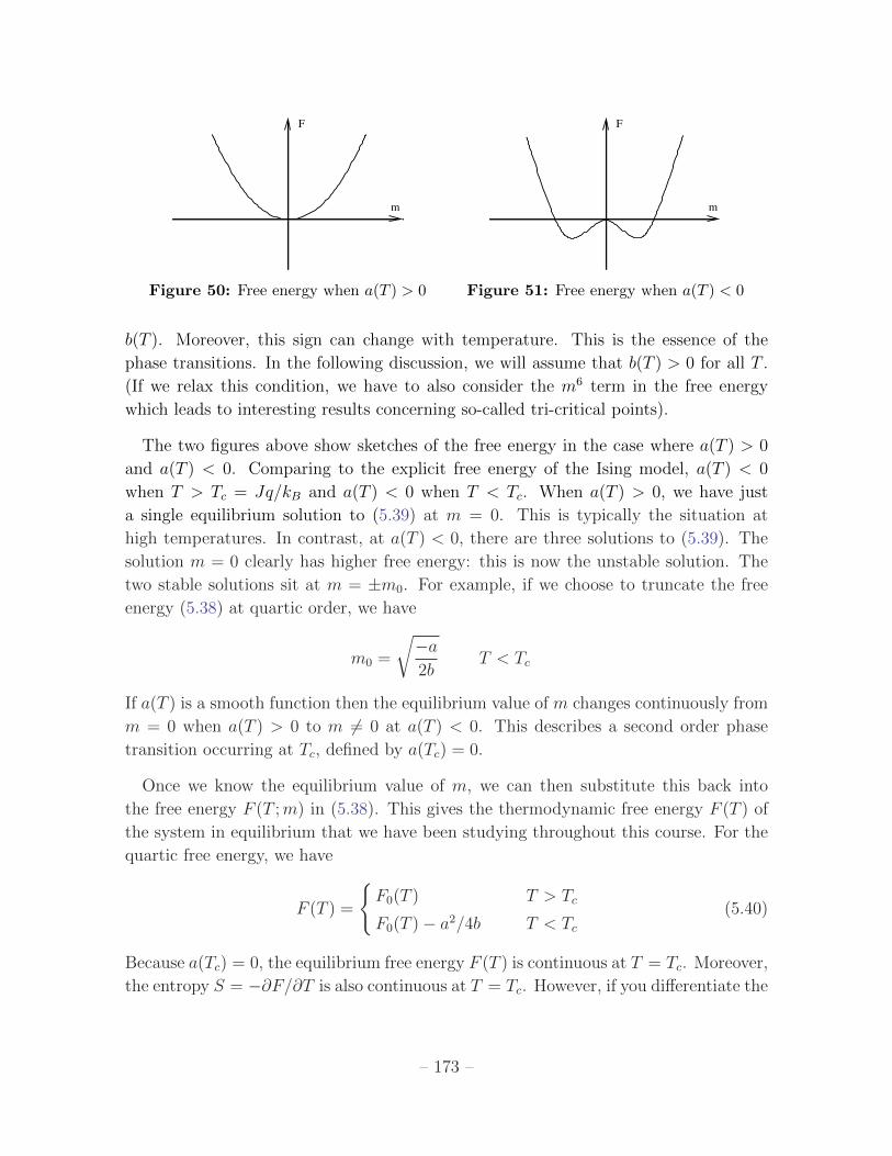
F
m
F
m
Figure 50: Free energy when a(T ) > 0 Figure 51: Free energy when a(T ) < 0
b(T ). Moreover, this sign can change with temperature. This is the essence of the
phase transitions. In the following discussion, we will assume that b(T ) > 0 for all T .
(If we relax this condition, we have to also consider the m6 term in the free energy
which leads to interesting results concerning so-called tri-critical points).
The two figures above show sketches of the free energy in the case where a(T ) > 0
and a(T ) < 0. Comparing to the explicit free energy of the Ising model, a(T ) < 0
when T > Tc = Jq/kB and a(T ) < 0 when T < Tc. When a(T ) > 0, we have just
a single equilibrium solution to (5.39) at m = 0. This is typically the situation at
high temperatures. In contrast, at a(T ) < 0, there are three solutions to (5.39). The
solution m = 0 clearly has higher free energy: this is now the unstable solution. The
two stable solutions sit at m = ±m0. For example, if we choose to truncate the free
energy (5.38) at quartic order, we have
m0 =
√−a2b
T < Tc
If a(T ) is a smooth function then the equilibrium value of m changes continuously from
m = 0 when a(T ) > 0 to m 6= 0 at a(T ) < 0. This describes a second order phase
transition occurring at Tc, defined by a(Tc) = 0.
Once we know the equilibrium value of m, we can then substitute this back into
the free energy F (T ;m) in (5.38). This gives the thermodynamic free energy F (T ) of
the system in equilibrium that we have been studying throughout this course. For the
quartic free energy, we have
F (T ) =
F0(T ) T > Tc
F0(T )− a2/4b T < Tc(5.40)
Because a(Tc) = 0, the equilibrium free energy F (T ) is continuous at T = Tc. Moreover,
the entropy S = −∂F/∂T is also continuous at T = Tc. However, if you differentiate the
– 173 –

equilibrium free energy twice, you will get a term a′ 2/b which is generically not vanishing
at T = Tc. This means that the heat capacity C = T∂S/∂T changes discontinuously
at T = Tc, as befits a second order phase transition. A word of warning: if you want to
compute equilibrium quantities such as the heat capacity, it’s important that you first
substitution in the equilibrium value of m and work with (5.40) rather than i (5.38).
If you don’t, you miss the fact that the magnetization also changes with T .
We can easily compute critical exponents within the context of Landau theory. We
need only make further assumptions about the behaviour of a(T ) and b(T ) in the
vicinity of Tc. If we assume that near T = Tc, we can write
b(T ) ≈ b0 , a(T ) ≈ a0(T − Tc) (5.41)
then we have
m0 ≈ ±√
a0
2b0
(Tc − T )1/2 T < Tc
which reproduces the critical exponent (5.9) and (5.20) that we derived for the van der
Waals equation and Ising model respectively.
Notice that we didn’t put any discontinuities into the free energy. Everything in
F (T ;m) was nice and smooth. When Taylor expanded, it has only integer powers of
m and T as shown in (5.38) and (5.41). But the minima of F behave in a non-analytic
fashion as seen in the expression for m0 above.
Landau’s theory of phase transitions predicts this same critical exponent for all values
of the dimension d of the system. But we’ve already mentioned in previous contexts
that the critical exponent is in fact only correct for d ≥ 4. We will understand how to
derive this criterion from Landau theory in the next section.
Spontaneous Symmetry Breaking
As we approach the end of the course, we’re touching upon a number of ideas that
become increasingly important in subsequent developments in physics. We already
briefly met the idea of universality and critical phenomena. Here I would like to point
out another very important idea: spontaneous symmetry breaking.
The free energy (5.38) is invariant under the Z2 symmetry m → −m. Indeed, we
said that one common reason that we can expand the free energy only in even powers
of m is that the underlying theory also enjoys this symmetry. But below Tc, the system
must pick one of the two ground states m = +m0 or m = −m0. Whichever choice it
makes breaks the Z2 symmetry. We say that the symmetry is spontaneously broken by
the choice of ground state of the theory.
– 174 –

Spontaneous symmetry breaking has particularly dramatic consequences when the
symmetry in question is continuous rather than discrete. For example, consider a
situation where the order parameter is a complex number ψ and the free energy is given
by (5.38) with m = |ψ|2. (This is effectively what happens for BECs, superfluids and
superconductors). Then we should only look at the m > 0 solutions so that the ground
state has |ψ|2 = +m0. But this leaves the phase of ψ completely undetermined. So
there is now a continuous choice of ground states: we get to sit anywhere on the circle
parameterised by the phase of ψ. Any choice that the system makes spontaneously
breaks the U(1) rotational symmetry which acts on the phase of ψ. Some beautiful
results due to Nambu and Goldstone show that the much of the physics of these systems
can be understood simply as a consequence of this symmetry breaking. The ideas of
spontaneous symmetry breaking are crucial in both condensed matter physics and
particle physics. In the latter context, it is intimately tied with the Higgs mechanism.
5.4.2 First Order Phase Transitions
Let us now consider a situation where the expansion of the free energy also includes
odd powers of the order parameter
F (T ;m) = F0(T ) + α(T )m+ a(T )m2 + γ(T )m3 + b(T )m4 + . . .
For example, this is the kind of expansion that we get for the Ising model free energy
(5.37) when B 6= 0, which reads
FIsing(T ;m) = −NkBT log 2 +JNq
2m2 − N
2kBT(B + Jqm)2 +
N
24(kBT )3(B + Jqm)4 + . . .
Notice that there is no longer a symmetry relating m → −m: the B field has a
preference for one sign over the other.
If we again assume that b(T ) > 0 for all temperatures, the crude shape of the free
energy graph again has two choices: there is a single minimum, or two minima and a
local maximum.
Let’s start at suitably low temperatures for which the situation is depicted in Figure
52. The free energy once again has a double well, except now slightly skewed. The local
maximum is still an unstable point. But this time around, the minima with the lower
free energy is preferred over the other one. This is the true ground state of the system.
In contrast, the point which is locally, but not globally, a minimum corresponds to a
meta-stable state of the system. In order for the system to leave this state, it must
first fluctuate up and over the energy barrier separating the two.
– 175 –

F F
m
F
m m
B<0 B=0 B>0
Figure 52: The free energy of the Ising model for B < 0, B = 0 and B > 0.
In this set-up, we can initiate a first order phase transition. This occurs when the
coefficient of the odd terms, α(T ) and γ(T ) change sign and the true ground state
changes discontinuously from m < 0 to m > 0. In some systems this behaviour
occurs when changing temperature; in others it could occur by changing some external
parameter. For example, in the Ising model the first order phase transition is induced
by changing B.
At very high temperature, the double well poten- F
m
Figure 53:
tial is lost in favour of a single minimum as depicted in
the figure to the right. There is a unique ground state, al-
beit shifted from m = 0 by the presence of the α(T ) term
above (which translates into the magnetic field B in the
Ising model). The temperature at which the meta-stable
ground state of the system is lost corresponds to the spin-
odial point in our discussion of the liquid-gas transition.
One can play further games in Landau theory, looking at how the shape of the free
energy can change as we vary temperature or other parameters. One can also use this
framework to give a simple explanation of the concept of hysteresis. You can learn
more about these from the links on the course webpage.
5.4.3 Lee-Yang Zeros
You may have noticed that the flavour of our discussion of phase transitions is a little
different from the rest of the course. Until now, our philosophy was to derive everything
from the partition function. But in this section, we dumped the partition function as
soon as we could, preferring instead to work with the macroscopic variables such as the
free energy. Why didn’t we just stick with the partition function and examine phase
transitions directly?
– 176 –

The reason, of course, is that the approach using the partition function is hard! In
this short section, which is somewhat tangential to our main discussion, we will describe
how phase transitions manifest themselves in the partition function.
For concreteness, let’s go back to the classical interacting gas of Section 2.5, although
the results we derive will be more general. We’ll work in the grand canonical ensemble,
with the partition function
Z(z, V, T ) =∑N
zNZ(N, V, T ) =∑N
zN
N !λ3N
∫ ∏i
d3ri e−β
∑j<k U(rjk) (5.42)
To regulate any potential difficulties with short distances, it is useful to assume that
the particles have hard-cores so that they cannot approach to a distance less than r0.
We model this by requiring that the potential satisfies
U(rjk) = 0 for rjk < r0
But this has an obvious consequence: if the particles have finite size, then there is a
maximum number of particles, NV , that we can fit into a finite volume V . (Roughly
this number is NV ∼ V/r30). But that, in turn, means that the canonical partition
function Z(N, V, T ) = 0 for N > NV , and the grand partition function Z is therefore
a finite polynomial in the fugacity z, of order NV . But if the partition function is a
finite polynomial, there can’t be any discontinuous behaviour associated with a phase
transition. In particular, we can calculate
pV = kBT logZ (5.43)
which gives us pV as a smooth function of z. We can also calculate
N = z∂
∂zlogZ (5.44)
which gives us N as a function of z. Eliminating z between these two functions (as
we did for both bosons and fermions in Section 3) tells us that pressure p is a smooth
function of density N/V . We’re never going to get the behaviour that we derived from
the Maxwell construction in which the plot of pressure vs density shown in Figure 37
exhibits a discontinous derivative.
The discussion above is just re-iterating a statement that we’ve alluded to several
times already: there are no phase transitions in a finite system. To see the discontinuous
behaviour, we need to take the limit V →∞. A theorem due to Lee and Yang12 gives
us a handle on the analytic properties of the partition function in this limit.12This theorem was first proven for the Ising model in 1952. Soon afterwards, the same Lee and
Yang proposed a model of parity violation in the weak interaction for which they won the 1957 Nobel
prize.
– 177 –
The surprising insight of Lee and Yang is that if you’re interested in phase transitions,
you should look at the zeros of Z in the complex z-plane. Let’s firstly look at these
when V is finite. Importantly, at finite V there can be no zeros on the positive real axis,
z > 0. This follows follows from the defintion of Z given in (5.42) where it is a sum
of positive quantities. Moreover, from (5.44), we can see that Z is a monotonically
increasing function of z because we necessarily have N > 0. Nonetheless, Z is a
polynomial in z of order NV so it certainly has NV zeros somewhere in the complex
z-plane. Since Z?(z) = Z(z?), these zeros must either sit on the real negative axis or
come in complex pairs.
However, the statements above rely on the fact that Z is a finite polynomial. As we
take the limit V →∞, the maximum number of particles that we can fit in the system
diverges, NV →∞, and Z is now defined as an infinite series. But infinite series can do
things that finite ones can’t. The Lee-Yang theorem says that as long as the zeros of Zcontinue to stay away from the positive real axis as V →∞, then no phase transitions
can happen. But if one or more zeros happen to touch the positive real axis, life gets
more interesting.
More concretely, the Lee-Yang theorem states:
• Lee-Yang Theorem: The quantity
Θ = limV→∞
(1
VlogZ(z, V, T )
)exists for all z > 0. The result is a continuous, non-decreasing function of z which
is independent of the shape of the box (up to some sensible assumptions such as
Surface Area/V ∼ V −1/3 which ensures that the box isn’t some stupid fractal
shape).
Moreover, let R be a fixed, volume independent, region in the complex z plane
which contains part of the real, positive axis. If R contains no zero of Z(z, V, T )
for all z ∈ R then Θ is a an analytic function of z for all z ∈ R. In particular, all
derivatives of Θ are continuous.
In other words, there can be no phase transitions in the region R even in the V →∞limit. The last result means that, as long as we are safely in a region R, taking
derivatives of with respect to z commutes with the limit V → ∞. In other words, we
are allowed to use (5.44) to write the particle density n = N/V as
limV→∞
n = limV→∞
z∂
∂z
(p
kBT
)= z
∂Θ
∂z
– 178 –

However, if we look at points z where zeros appear on the positive real axis, then Θ will
generally not be analytic. If dΘ/dz is discontinuous, then the system is said to undergo
a first order phase transition. More generally, if dmΘ/dzm is discontinuous for m = n,
but continuous for all m < n, then the system undergoes an nth order phase transition.
We won’t offer a proof of the Lee-Yang theorem. Instead illustrate the general idea
with an example.
A Made-Up Example
Ideally, we would like to start with a Hamiltonian which exhibits a first order phase
transition, compute the associated grand partition function Z and then follow its zeros
as V → ∞. However, as we mentioned above, that’s hard! Instead we will simply
make up a partition function Z which has the appropriate properties. Our choice is
somewhat artificial,
Z(z, V ) = (1 + z)[αV ](1 + z[αV ])
Here α is a constant which will typically depend on temperature, although we’ll suppress
this dependence in what follows. Also,
[x] = Integer part of x
Although we just made up the form of Z, it does have the behaviour that one would
expect of a partition function. In particular, for finite V , the zeros sit at
z = −1 and z = eπi(2n+1)/[αV ] n = 0, 1, . . . , [αV ]− 1
As promised, none of the zeros sit on the positive real axis.However, as we increase V ,
the zeros become denser and denser on the unit circle. From the Lee-Yang theorem,
we expect that no phase transition will occur for z 6= 1 but that something interesting
could happen at z = 1.
Let’s look at what happens as we send V →∞. We have
Θ = limV→∞
1
VlogZ(z, V )
= limV→∞
1
V
([αV ] log(1 + z) + log(1 + z[αV ])
)=
α log(1 + z) |z| < 1
α log(1 + z) + α log z |z| > 1
We see that Θ is continuous for all z as promised. But it is only analytic for |z| 6= 1.
– 179 –

We can extract the physics by using (5.43) and (5.44) to eliminate the dependence
on z. This gives us the equation of state, with pressure p as a function of n = V/N .
For |z| < 1, we have
p = αkBT log
(α
α− n
)n ∈ [0, α/2) , p < kBT log 2
While for |z| > 1, we have
p = αkBT log
(2αn
(2α− n)2
)n ∈ (3α/2, 2α) , p > kBT log 2
They key point is that there is a jump in particle density of ∆n = α at p = αkBT log 2.
Plotting this as a function of p vs v = 1/n, we find that we have a curve that is qualita-
tively identical to the pressure-volume plot of the liquid-gas phase diagram under the
co-existence curve. (See, for example, figure 37). This is a first order phase transition.
5.5 Landau-Ginzburg Theory
Landau’s theory of phase transition focusses only on the average quantity, the order
parameter. It ignores the fluctuations of the system, assuming that they are negligible.
Here we sketch a generalisation which attempts to account for these fluctuations. It is
known as Landau-Ginzburg theory.
The idea is to stick with the concept of the order parameter, m. But now we allow
the order parameter to vary in space so it becomes a function m(~r). Let’s restrict
ourselves to the situation where there is a symmetry of the theory m → −m so we
need only consider even powers in the expansion of the free energy. We add to these
a gradient term whose role is to captures the fact that there is some stiffness in the
system, so it costs energy to vary the order parameter from one point to another. (For
the example of the Ising model, this is simply the statement that nearby spins want to
be aligned). The free energy is then given by
F [m(~r)] =
∫ddr
[a(T )m2 + b(T )m4 + c(T )(∇m)2
](5.45)
where we have dropped the constant F0(T ) piece which doesn’t depend on the order
parameter and hence plays no role in the story. Notice that we start with terms
quadratic in the gradient: a term linear in the gradient would violate the rotational
symmetry of the system.
– 180 –

We again require that the free energy is minimised. But now F is a functional – it is
a function of the function m(~r). To find the stationary points of such objects we need
to use the same kind of variational methods that we use in Lagrangian mechanics. We
write the variation of the free energy as
δF =
∫ddr
[2amδm+ 4bm3 δm+ 2c∇m · ∇δm
]=
∫ddr
[2am+ 4bm3 − 2c∇2m
]δm
where to go from the first line to the second we have integrated by parts. (We need
to remember that c(T ) is a function of temperature but does not vary in space so
that ∇ doesn’t act on it). The minimum of the free energy is then determined by
setting δF = 0 which means that we have to solve the Euler-Lagrange equations for
the function m(~r),
c∇2m = am+ 2bm3 (5.46)
The simplest solutions to this equation have m constant, reducing us back to Landau
theory. We’ll assume once again that a(T ) > 0 for T > Tc and a(T ) < 0 for T < Tc.
Then the constant solutions are m = 0 for T > Tc and m = ±m0 = ±√−a/2b for
T < Tc. However, allowing for the possibility of spatial variation in the order parameter
also opens up the possibility for us to search for more interesting solutions.
Domain Walls
Suppose that we have T < Tc so there exist two degenerate ground states, m = ±m0.
We could cook up a situation in which one half of space, say x < 0, lives in the ground
state m = −m0 while the other half of space, x > 0 lives in m = +m0. This is exactly
the situation that we already met in the liquid-gas transition and is depicted in Figure
38. It is also easy to cook up the analogous configuration in the Ising model. The two
regions in which the spins point up or down are called domains. The place where these
regions meet is called the domain wall.
We would like to understand the structure of the domain wall. How does the system
interpolate between these two states? The transition can’t happen instantaneously
because that would result in the gradient term (∇m)2 giving an infinite contribution
to the free energy. But neither can the transition linger too much because any point at
which m(~r) differs significantly from the value m0 costs free energy from the m2 and
m4 terms. There must be a happy medium between these two.
– 181 –

To describe the system with two domains, m(~r) must vary but it need only change
in one direction: m = m(x). Equation (5.46) then becomes an ordinary differential
equation,
d2m
dx2=am
c+
2bm3
c
This equation is easily solved. We should remember that in order to have two vacua,
T < Tc which means that a < 0. We then have
m = m0 tanh
(√−a2cx
)
where m0 =√−a/2b is the constant ground state solution for the spin. As x→ ±∞,
the tanh function tends towards ±1 which means that m → ±m0. So this solution
indeed interpolates between the two domains as required. We learn that the width of
the domain wall is given by√−2c/a. Outside of this region, the magnetisation relaxes
exponentially quickly back to the ground state values.
We can also compute the cost in free energy due to the presence of the domain wall.
To do this, we substitute the solution back into the expression for the free energy (5.45).
The cost is not proportional to the volume of the system, but instead proportional to
the area of the domain wall. This means that if the system has linear size L then the
free energy of the ground state scales as Ld while the free energy required by the wall
scales only as Ld−1. It is simple to find the parametric dependence of this domain wall
energy without doing any integrals; the energy per unit area scales as√−ca3/b. Notice
that as we approach the critical point, and a→ 0, the two vacua are closer, the width
of the domain wall increases and its energy decreases.
5.5.1 Correlations
One of the most important applications of Landau-Ginzburg theory is to understand
the correlations between fluctuations of the system at different points in space. Suppose
that we know that the system has an unusually high fluctuation away from the average
at some point in space, let’s say the origin ~r = 0. What is the effect of this on nearby
points?
There is a simple way to answer this question that requires us only to solve the
differential equation (5.46). However, there is also a more complicated way to derive
the same result which has the advantage of stressing the underlying physics and the
role played by fluctuations. Below we’ll start by deriving the correlations in the simple
manner. We’ll then see how it can also be derived using more technical machinery.
– 182 –
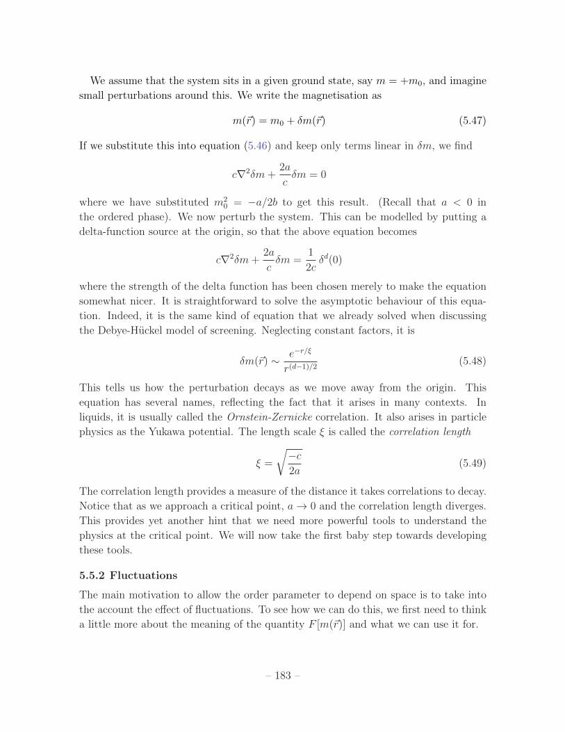
We assume that the system sits in a given ground state, say m = +m0, and imagine
small perturbations around this. We write the magnetisation as
m(~r) = m0 + δm(~r) (5.47)
If we substitute this into equation (5.46) and keep only terms linear in δm, we find
c∇2δm+2a
cδm = 0
where we have substituted m20 = −a/2b to get this result. (Recall that a < 0 in
the ordered phase). We now perturb the system. This can be modelled by putting a
delta-function source at the origin, so that the above equation becomes
c∇2δm+2a
cδm =
1
2cδd(0)
where the strength of the delta function has been chosen merely to make the equation
somewhat nicer. It is straightforward to solve the asymptotic behaviour of this equa-
tion. Indeed, it is the same kind of equation that we already solved when discussing
the Debye-Huckel model of screening. Neglecting constant factors, it is
δm(~r) ∼ e−r/ξ
r(d−1)/2(5.48)
This tells us how the perturbation decays as we move away from the origin. This
equation has several names, reflecting the fact that it arises in many contexts. In
liquids, it is usually called the Ornstein-Zernicke correlation. It also arises in particle
physics as the Yukawa potential. The length scale ξ is called the correlation length
ξ =
√−c2a
(5.49)
The correlation length provides a measure of the distance it takes correlations to decay.
Notice that as we approach a critical point, a→ 0 and the correlation length diverges.
This provides yet another hint that we need more powerful tools to understand the
physics at the critical point. We will now take the first baby step towards developing
these tools.
5.5.2 Fluctuations
The main motivation to allow the order parameter to depend on space is to take into
the account the effect of fluctuations. To see how we can do this, we first need to think
a little more about the meaning of the quantity F [m(~r)] and what we can use it for.
– 183 –

To understand this point, it’s best if we go back to basics. We know that the true
free energy of the system can be equated with the log of the partition function (1.36).
We’d like to call the true free energy of the system F because that’s the notation that
we’ve been using throughout the course. But we’ve now called the Landau-Ginzburg
functional F [m(~r)] and, while it’s closely related to the true free energy, it’s not quite
the same thing as we shall shortly see. So to save some confusion, we’re going to change
notation at this late stage and call the true free energy A. Equation (1.36) then reads
A = −kBT logZ, which we write this as
e−βA = Z =∑n
e−βEn
We would like to understand the right way to view the functional F [m(~r)] in this frame-
work. Here we give a heuristic and fairly handwaving argument. A fuller treatment
involves the ideas of the renormalisation group.
The idea is that each microstate |n〉 of the system can be associated to some specific
function of the spatially varying order parameter m(~r). To illustrate this, we’ll talk
in the language of the Ising model although the discussion generalises to any system.
There we could consider associate a magnetisation m(~r) to each lattice site by simply
averaging over all the spins within some distance of that point. Clearly, this will only
lead to functions that take values on lattice sites rather than in the continuum. But if
the functions are suitably well behaved it should be possible to smooth them out into
continuous functions m(~r) which are essentially constant on distance scales smaller
than the lattice spacing. In this way, we get a map from the space of microstates to
the magnetisation, |n〉 7→ m(~r). But this map is not one-to-one. For example, if the
averaging procedure is performed over enough sites, flipping the spin on just a single
site is unlikely to have much effect on the average. In this way, many microstates map
onto the same average magnetisation. Summing over just these microstates provides a
first principles construction of the F [m(~r)],
e−βF [m(~r)] =∑n|m(~r)
e−βEn (5.50)
Of course, we didn’t actually perform this procedure to get to (5.45): we simply wrote it
down the most general form in the vicinity of a critical point with a bunch of unknown
coefficients a(T ), b(T ) and c(T ). But if we were up for a challenge, the above procedure
tells us how we could go about figuring out those functions from first principles. More
importantly, it also tells us what we should do with the Landau-Ginzburg free energy.
Because in (5.50) we have only summed over those states that correspond to a particular
– 184 –
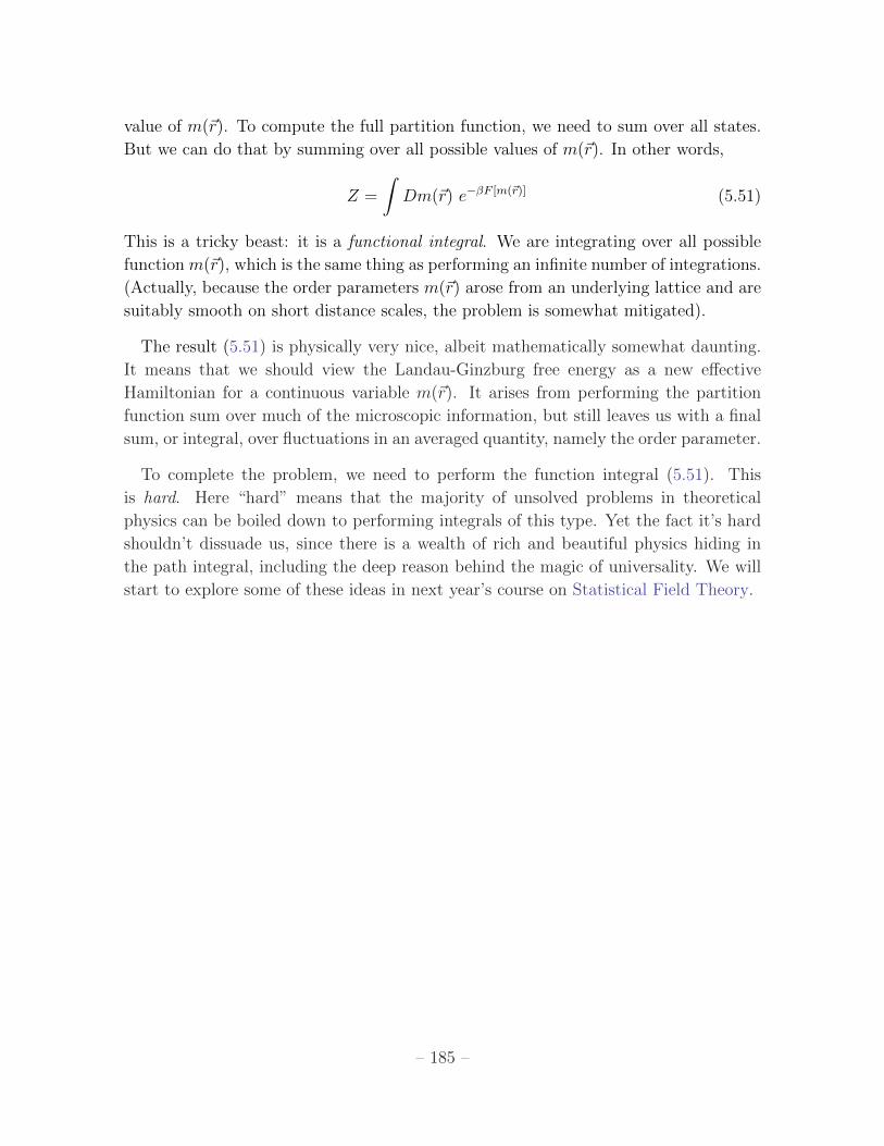
value of m(~r). To compute the full partition function, we need to sum over all states.
But we can do that by summing over all possible values of m(~r). In other words,
Z =
∫Dm(~r) e−βF [m(~r)] (5.51)
This is a tricky beast: it is a functional integral. We are integrating over all possible
function m(~r), which is the same thing as performing an infinite number of integrations.
(Actually, because the order parameters m(~r) arose from an underlying lattice and are
suitably smooth on short distance scales, the problem is somewhat mitigated).
The result (5.51) is physically very nice, albeit mathematically somewhat daunting.
It means that we should view the Landau-Ginzburg free energy as a new effective
Hamiltonian for a continuous variable m(~r). It arises from performing the partition
function sum over much of the microscopic information, but still leaves us with a final
sum, or integral, over fluctuations in an averaged quantity, namely the order parameter.
To complete the problem, we need to perform the function integral (5.51). This
is hard. Here “hard” means that the majority of unsolved problems in theoretical
physics can be boiled down to performing integrals of this type. Yet the fact it’s hard
shouldn’t dissuade us, since there is a wealth of rich and beautiful physics hiding in
the path integral, including the deep reason behind the magic of universality. We will
start to explore some of these ideas in next year’s course on Statistical Field Theory.
– 185 –
Related Documents


