Statistical Modeling in the Wavelet Domain and Applications by Roland Kwitt A thesis submitted to the Department of Computer Sciences at the University of Salzburg in partial fulfillment of the requirements for the degree of Dr. techn. April 2010 Supervisor: Ao. Prof. Dr. Mag. rer. nat. Andreas Uhl Department of Computer Sciences University of Salzburg, Salzburg, Austria External Reviewer: Prof. Dr. Nick G. Kingsbury Department of Engineering University of Cambridge, Cambridge, United Kingdom

Welcome message from author
This document is posted to help you gain knowledge. Please leave a comment to let me know what you think about it! Share it to your friends and learn new things together.
Transcript

Statistical Modeling in the Wavelet Domain
and Applications
byRoland Kwitt
A thesis submitted to theDepartment of Computer Sciences at the
University of Salzburgin partial fulfillment of the requirements
for the degree of Dr. techn.
April 2010
Supervisor: Ao. Prof. Dr. Mag. rer. nat. Andreas UhlDepartment of Computer Sciences
University of Salzburg, Salzburg, Austria
External Reviewer: Prof. Dr. Nick G. KingsburyDepartment of Engineering
University of Cambridge, Cambridge, United Kingdom

Abstract
In this thesis, we study statistical models for transform coefficients of two different wavelettransform variants, the pyramidal Discrete Wavelet Transform (DWT) and the Dual-Tree Com-plex Wavelet Transform (DTCWT). The work is motivated by the high computational demandof many state-of-the-art modeling approaches, although a variety of applications require com-putationally efficient, yet accurate models which facilitate straightforward parameter estima-tion and possess an analytically tractable form. In case of the DTCWT, there is also very littleliterature on (joint) statistical modeling of complex wavelet coefficients, even though it is a well-established fact that complex wavelet transforms exhibit striking advantages compared to theDWTwhen it comes to image analysis applications. The statistical models we develop through-out this thesis are utilized in three different areas of image processing. We address the researchbranches of (probabilistic) texture image retrieval, medical image classification and image wa-termarking. For each particular field, we provide a brief introduction of the problem, thenintroduce our contribution and conclude with an extensive experimental section. This includesa comparative study to existing work in literature and, depending on whether computationaleffort is a crucial issue, a thorough computational analysis of the main building blocks. Our re-sults reveal, that the proposed models are beneficial in the aforementioned areas and improveupon state-of-the-art work. In addition, application of statistical models is not limited to thepresented fields. In fact, we presume that other areas of transform domain based image pro-cessing, such as denoising or segmentation, can benefit in a similar manner.

Acknowledgements
This thesis is devoted to my parents, Richard and Monika, and my girlfriend Daniela. Spe-cial thanks goes to my advisor Andreas Uhl for providing magnificent support and guidingthroughout my PhD studies. I also like to thank my second advisor Karl Entacher and myco-worker Peter Meerald for great collaborations and many productive discussions in the lastyears. Eventually, I like to give thanks to the Austrian Science Fund (FWF) for funding thisthesis under project no. L366-N15.

Contents
Contents 3
1 Introduction 5
1.1 Contribution . . . . . . . . . . . . . . . . . . . . . . . . . . . . . . . . . . . . . . . . 61.2 Organization . . . . . . . . . . . . . . . . . . . . . . . . . . . . . . . . . . . . . . . . 81.3 Image Databases . . . . . . . . . . . . . . . . . . . . . . . . . . . . . . . . . . . . . 81.4 Notational Conventions . . . . . . . . . . . . . . . . . . . . . . . . . . . . . . . . . 91.5 Some Notes on Reproducibility . . . . . . . . . . . . . . . . . . . . . . . . . . . . . 9
2 Statistical Modeling in the Wavelet Domain 11
2.1 The Statistical Toolset . . . . . . . . . . . . . . . . . . . . . . . . . . . . . . . . . . . 112.2 DWT Subband Models . . . . . . . . . . . . . . . . . . . . . . . . . . . . . . . . . . 122.3 Complex Wavelet Transform Subband Models . . . . . . . . . . . . . . . . . . . . 31
3 Texture Image Retrieval 47
3.1 Image Retrieval as Statistical Inference . . . . . . . . . . . . . . . . . . . . . . . . . 483.2 Related Work . . . . . . . . . . . . . . . . . . . . . . . . . . . . . . . . . . . . . . . 503.3 Lightweight Probabilistic Texture Retrieval . . . . . . . . . . . . . . . . . . . . . . 513.4 Copula-Based Retrieval . . . . . . . . . . . . . . . . . . . . . . . . . . . . . . . . . 623.5 Discussion . . . . . . . . . . . . . . . . . . . . . . . . . . . . . . . . . . . . . . . . . 68
4 Medical Image Classification 69
4.1 The Medical Presentation of the Problem . . . . . . . . . . . . . . . . . . . . . . . 704.2 Prediction by Means of Discriminant Classifiers . . . . . . . . . . . . . . . . . . . 724.3 Prediction by Means of Generative Models . . . . . . . . . . . . . . . . . . . . . . 784.4 Classification Setup . . . . . . . . . . . . . . . . . . . . . . . . . . . . . . . . . . . . 794.5 Experiments . . . . . . . . . . . . . . . . . . . . . . . . . . . . . . . . . . . . . . . . 804.6 Discussion . . . . . . . . . . . . . . . . . . . . . . . . . . . . . . . . . . . . . . . . . 90
5 Watermarking 92
5.1 Watermarking as a Signal Detection Problem . . . . . . . . . . . . . . . . . . . . . 935.2 A Rao Hypothesis Test for Cauchy Host Signal Noise . . . . . . . . . . . . . . . . 995.3 Color Image Watermarking . . . . . . . . . . . . . . . . . . . . . . . . . . . . . . . 107
3

Contents 4
5.4 Discussion . . . . . . . . . . . . . . . . . . . . . . . . . . . . . . . . . . . . . . . . . 112
6 Concluding Remarks 115
6.1 Future Research Directions . . . . . . . . . . . . . . . . . . . . . . . . . . . . . . . . 116
References 117
Chapter 1
Introduction
In many disciplines of scientific research, measurements or observations in general make upthe basis for any processing step. It is not uncommon to assume that these measurements stemfrom some underlying stochastic process. Consequently, many problems can be formulated asproblems of statistical inference. At the very core of inferential procedures, we identify suitablestatistical models which capture certain characteristics of the observations. In this thesis, we areparticularly concerned with statistical inference problems which arise in the context of imageprocessing. To be more specific, we focus on the area of transform domain image processing,where the wavelet transform in all of its variants has proved to be highly beneficial. In fact, thewavelet transform resembles the way our visual system processes information which makes itvery attractive from an image processing point of view. The basic motivation for leaving thepixel domain and switching to a transform domain representation of images is to facilitate anykind of processing operations. Throughout the last years, statistical models for wavelet trans-form coefficients have found application in many areas of image processing, such as denoising[16, 127, 155], coding [164, 110], compression [14], classification [18, 106], image retrieval [40] orwatermarking [69, 139, 12].
The pyramidal Discrete Wavelet Transform (DWT) [113, 114] is by far the most prevalenttransformation in the image processing community. In a similar manner, the coverage of sta-tistical models for DWT coefficients is quite extensive [71, 155, 190, 109]. Nevertheless, theDWT is not tailored for image analysis applications (i.e. classification, denoising, etc.) andeven has some well-known deficiencies in this context. To overcome the shortcomings of theDWT, many alternative transformations have been developed recently, however, only a smallsubset has gained substantial interest in the community. Two of these alternatives are theSteerable Pyramid of Simoncelli et al. [168] and the Dual-Tree Complex Wavelet Transform(DTCWT), proposed by Kingsbury [85]. Since the transform coefficient statistics of coefficientsfrom the Steerable Pyramid resemble the statistics of DWT coefficients, many works have beendevoted to the development of suitable statistical models for Steerable Pyramid coefficients aswell [190, 39, 179]. In contrast, the number of publications dealing with statistical models forDTCWT coefficients is substantially lower [163, 154, 19, 151]. Most works focus on modelsfor the magnitudes of complex wavelet coefficients, however, recently the phase has gained
5

Chapter 1. Introduction 6
research interest as well [128, 129, 189].The motivation for developing novel statistical models for wavelet coefficients has several
facets. In case of the DWT, our motivation is strongly related to the area of transform domainwatermarking [28]. We identify two topics which received little treatment in literature so far.First, the commonly-accepted model for DWT coefficients, the Generalized Gaussian distribu-tion [22] has the disadvantage of computationally expensive and numerically cumbersome pa-rameter estimation [97]. Unless the model parameters are set to predefined values (see, e.g.[69]) – which might have a negative impact on detector performance – this fact prevents the useof a GGD-based detector in computationally demanding scenarios. As an alternative, we seeka statistical model which allows to derive a watermark detector with an analytically tractableform and a computationally inexpensive way to estimate the model parameters. This modelmight be less appropriate in terms of Goodness-of-Fit, yet accurate enough to outperform thestandard Gaussian distribution in terms of watermark detection performance. As a secondpoint, we highlight the fact that statistical models tailored to capture the association betweenDWT coefficients are primarily based on Hidden Markov models [155, 109]. Although, thisallows to model inter- and intra-scale dependencies, those models turn out to be analyticallyintractable in Likelihood-Ratio testing scenarios. Since we want to facilitate color image water-marking in the wavelet transform domain, extending the Hidden Markov model approach tocolor images [192] is unrewarding. Instead, we seek a joint statistical model which can capturecoefficient dependencies across color channels and yet allows to derive closed-form expressionsfor Likelihood-Ratio tests.
Regarding the development of statistical models for DTCWT coefficients, our motivationstems from a completely different research area. We are concerned with a medical image classi-fication problem which bears a strong relation to the field of texture image retrieval and classi-fication. Our intention is to evaluate whether statistical approaches to capture coefficient char-acteristics are equally effective for our medical problem as they are in texture analysis applica-tions, see e.g. [150, 40, 179]. Our objective is to advance existing statistical models for DTCWTcoefficient magnitudes and to quantify the suitability of the models with respect to classificationand texture retrieval performance. Since both problems have strong computational constraints,we aim for analytically tractable approaches and straightforward parameter estimation. In ad-dition, we are further motivated to develop a computationally simple alternative to the HiddenMarkov Tree approach of [19] in order to capture DTCWT coefficient dependencies, especiallyacross color channels. This seems a promising idea in consideration of the fact that color infor-mation has shown to be beneficial in texture discrimination scenarios [35].
1.1 Contribution
The contribution of this thesis is split into several parts. Basically, we discuss several statisticalmodels for DWT and DTCWT coefficients and their application in three different areas of imageprocessing. In the context of DWT coefficient modeling, we briefly review the popular Gener-alized Gaussian model and the less often used Cauchy distribution. The latter model is thenused in the context of image watermarking to derive a computationally efficient watermarkdetector which exhibits substantially better detection performance than several state-of-the-artdetectors on a large set of natural images. In order to incorporate coefficient dependenciesamong the subbands of DWT decomposed color channels into the watermark detection pro-cess, we present a joint statistical model which can be considered as a multivariate extension tothe Generalized Gaussian distribution. We deal with parameter estimation issues and suggest

Chapter 1. Introduction 7
a novel Goodness-of-Fit test to quantify the suitability of the model. In an extensive size andpower study we show that the desired significance levels can be met and that the test exhibitsremarkable power against shape alternatives. Eventually, we derive a novel watermark detec-tor based on the joint statistical model and demonstrate that our detector performs better thantwo state-of-the-art detectors in field of color image watermarking.
In the context of DTCWT coefficient modeling, we advance current research results to theeffect that we present two novel models for subband coefficient magnitudes which are bothaccurate and admit straightforward parameter estimation. We quantify the suitability of theproposed models by means of an extensive Goodness-of-Fit study on four commonly-used tex-ture image databases. The modeling results are then exploited for lightweight texture imageretrieval where we propose a novel retrieval approach based on a probabilistic formulationof image retrieval [186]. We show that switching from computationally expensive Maximum-Likelihood parameter estimation procedures to moment matching approaches does not nega-tively affect the retrieval rates, however considerably lowers the computational burden of thisstep. A computational analysis of the main building blocks of the retrieval framework confirmsthat we can design a probabilistic approach with low computational complexity. In contrast tothe majority of research papers on texture image retrieval, we conduct an extensive compara-tive retrieval study on four texture image repositories to evaluate the quality of our proposedapproach with respect to several state-of-the-art approaches.
In a second step of modeling the DTCWT coefficient magnitudes, we present an alternativemodel to the Hidden Markov Tree approach of [19]. Since DTCWT coefficients exhibit a quitestrong association structure, it appears reasonable to capture this association by a joint statisticalmodel. For that purpose, we propose a copula-based approach which (i) allows to rely onexisting knowledge about the DTCWT coefficient statistics and (ii) completely separates thetask of finding a suitable model for the association structure. We show, that the copula-basedmodel for DTCWT coefficients can be exploited for texture image retrieval and perfectly fits intothe probabilistic framework we mentioned above. Again, we can demonstrate a considerableincrease in retrieval performance, however, at the expense of computation time. To remedythis shortcoming, we suggest a simple data reduction strategy which only slightly affects theretrieval results, but allows to deploy the approach even on large databases.
As a third field of application, we tackle the medical image processing problem of predictinghistologies from colonoscopy images based on the visual appearance of the mucosal surface pat-terns. We demonstrate, that a computer-assisted prediction system can be a serious diagnostictool for in vivo staging of colorectal lesions. In particular, we consider two different strategies tocope with that problem. First, we take the straightforwardway of using a discriminant classifierapproach. Second, we consider the prediction problem from the viewpoint of image retrievaland discuss the advantages of a generative model based approach. In the former case, we ex-ploit the statistical models for DTCWT coefficient magnitudes to construct feature vectors basedon the estimated model parameters. Then, we extend the concept of co-occurrence matrices (see[65, 148]) to capture the joint occurrence of wavelet coefficients across different color channelsand compute a set of commonly-used texture descriptors from these matrices. Eventually, wepresent an approach of decorrelating wavelet subbands from different color channels and usingthe variances of the decorrelated subbands as image features. In all three cases, classificationis based on a nearest-neighbor principle and we demonstrate remarkable classification rates fortwo clinically relevant scenarios. In the context of generative models, we highlight potentialdisadvantages of discriminant classifier based approaches and emphasize the points where aretrieval oriented point of view can be beneficial. We present impressive prediction results for

Chapter 1. Introduction 8
the image retrieval approaches with similar or higher rates compared to human-based studies.
1.2 Organization
In the remaining part of this introductory chapter, we include a brief discussion of the four im-age databases we use throughout the thesis. Further, we provide some notational conventionsand address the topic of reproducible research. The remaining chapters are then organizedinto two major parts: in the first part, i.e. Chapter 2, we develop the statistical foundation ofthe following chapters. The second part is devoted to the areas of application of the differentstatistical models. Each application-specific chapter is structured in a similar way: first, we in-troduce the presentation of the problem, then we present our contribution and conclude withan experimental evaluation and a brief discussion of the results. Since the fields of applicationspan different research areas, it is unrewarding to devote a separate chapter to related researchwork. We rather follow the strategy to establish connections to previous works as we progressfrom chapter to chapter. In Chapter 3, we revisit a recently proposed formulation of probabilis-tic image retrieval and then exploit the statistical models for DTCWT coefficients to developtwo novel retrieval approaches. Chapter 4 is devoted to the medical image classification prob-lem and Chapter 5 deals with the topic of image watermarking. Chapter 6 concludes the thesiswith a confrontation of the original questions and the achieved results. Finally, we provide anoutlook on open research problems and topics we could not cover in this thesis.
1.3 Image Databases
Image databases constitute the basis for all experimental results presented throughout this the-sis. We use one database of natural images (UCID [159]) and three databases of texture images.The three texture databases consist of two commonly-known repositories (Outex [142] and Vis-tex [31]), and one real-world database of textures captured by the author and several cowork-ers1 (Stex). We consciously exclude two other popular databases, the Brodatz album [13] andthe CUReT [30] textures for several reasons: first, availability of the Brodatz album is limited tograyscale images2 and the amount of available textures differs in literature (111 in [149], 112 in[186] or even 116 in [111]). Second, CURet3 only provides a set of 61 different physical textures,however, under 205 different viewpoint and illumination combinations. Since we already usethe Outex database which contains textures captured under artificial conditions, we choose notto include another database of this kind. Example images from all four databases are shownin Fig. 1.1 including some commonly-known example images (i.e. Fig. 1.1a) we often use forillustration purposes.
UCID Summarizing the description of Schaefer & Stich [159], the UCID image database con-sists of 1338 images in uncompressed form (TIFF format) captured by a Minolta Dimage5 camera. All images are either 512 × 384 or 384 × 512 pixel and were captured usingautomatic settings which mostly resembles a real-world scenario.
Outex Since the test suite for texture retrieval in the Outex database only consists of grayscaleimages of size 128 × 128 pixel, we first fetched 316 color texture images in BMP format
1thanks to Heinz Hofbauer, Stefan Huber, Peter Meerwald and Daniela Wöckinger2available from http://www.ux.uis.no/~tranden/brodatz.html3available from http://www.cs.columbia.edu/CAVE/software/curet

Chapter 1. Introduction 9
with 600dpi under inca lightning conditions from the Outex website4. Two images,canvas007, canvas010 were missing, wallpaper015 was not accessible. The imageswere then cropped to 512× 512 pixel starting from the top-left hand corner of the image.
Vistex We use the original 512×512 pixel versions of the texture images available from the MITVision Texture website5. There are 167 textures available, denoted by Vistex (full). Wefurther select a subset of 40 textures, denoted by Vistex (small), since many approachesin various publications (see, e.g. [40, 101, 188]) use this limited subset. According to theinformation on the website, images in the Vistex databasewere captured under real-worldconditions without studio lightning.
Stex The Stex database is a novel texture database consisting of 476 images of different tex-tures captured in the area around Salzburg/Austria using three cameras: a Canon IXUS70, a Canon EOS 450D and a Nikon D40. Similar to the Vistex database, our image setis intended to resemble a real-life scenario. Except for the Canon EOS 450D pictureswhich were captured in RAW format, all other textures were stored as JPEG images. Post-processing consisted of conversion to PNM format (using the ImageMagick’s converttool) and resizing to 512× 512 pixels by means of bicubic interpolation (using MATLABsimresize routine).
1.4 Notational Conventions
To reach maximum notational consistency, we have to introduce some conventions. First, if notstated otherwise, uppercase letters (i.e. X) will be used to denote random variables. Lowercaseletters (i.e. x) will denote observations. Accordingly, boldface uppercase letters denote randomvectors (i.e. X). In case X denotes a matrix, the meaning will be unambiguous from the context.Lowercase boldface letters (i.e. x) will denote observation vectors. We adhere to the conventionthat FX denotes the cumulative distribution function (c.d.f.) of a random variable X and pX
denotes the corresponding probability density function (p.d.f) or the probability mass function(p.m.f.) in case of discrete random variables. Greek letters, such as α or α denote parameters orparameter vectors, respectively. Entities, such as images, will be denoted by calligraphic letters(i.e. I). When we speak of an image database, we mean a collection of images I1, . . . , IL of sizeL. Regarding the use of special functions, Γ denotes the Gamma function and ψ denotes theDigamma function [1]. All further notational conventions will be introduced at the correspond-ing locations.
1.5 Some Notes on Reproducibility
As Vandewalle et al. (see [181] and references therein) recently pointed out, reproducible re-search is at the very core of every scientific discipline. In order to reach a certain degree ofreproducibility of the results presented in this thesis, we provide reference implementations ofall approaches as either C or MATLAB code6. Further, we provide access to the Stex databaseas another reference repository to evaluate texture analysis algorithms. Unfortunately, access tothe medical database we use in Chapter 4 is restricted due to privacy issues.
4available from http://www.outex.oulu.fi/5available from http://vismod.media.mit.edu/vismod/imagery/VisionTexture/6available from http://www.wavelab.at/sources

Chapter 1. Introduction 10
(a) Some classic example images: Lena, Elaine, Bridge, Boat, Peppers and Barbara.
(b) Vistex
(c) Outex
(d) Stex
(e) UCID
Figure 1.1: Example images from different image databases.

Chapter 2
Statistical Modeling in the Wavelet Domain
In this chapter, we discuss the foundation of this thesis, namely the statistical models of waveletcoefficients from two different wavelet transforms. We start with an introduction of a set ofstatistical tools which we extensively use in the following sections. Other statistical procedureswhich are used in this thesis will be introduced when needed. After this brief introduction,the chapter is basically split into two parts: in the first part, we recapitulate the main results onstatistical modeling of DiscreteWavelet Transform (DWT) coefficients, and in particular, we takea closer look at the characteristic distributions which arise in case of natural images. Then, wepresent a novel multivariate model to capture the dependencies across DWT detail subbands ofdifferent color channels and develop a novel Goodness of Fit test for this multivariate model. Inthe second part, we continue with a discussion of characteristic coefficient distributions whicharise when we decompose images by means of a complex wavelet transform variant, knownas the Dual-Tree Complex Wavelet Transform (DTCWT). We particularly focus on statisticalmodels for DTCWT transform coefficient magnitudes of texture images. Finally, we presenta multivariate extension to the univariate models in order to capture coefficient dependenciesacross subbands and color channels.
2.1 The Statistical Toolset
A commonly observed situation in the first stage of finding a suitable statistical model for aset of (univariate) observations is to analyze the frequency distribution. Usually, a classic his-togram is used as a first choice where the range of observation values is divided into a certainnumber of bins (with equal bin width) and we count the number of observations falling intoeach bin. Plotting the bins against the bin count then conveys an impression about the fre-quency distribution. However, in case our objective is to highlight certain characteristics ofthe observations such as tail behavior for instance, other variants of the classic histogram aremore reasonable. In situations where we expect heavy tails for example, it has become commonpractice to visualize the y-axis of the histogram on a logarithmic scale. We refer to this type ofhistogram as the log-scale histogram. In order to check the Goodness of Fit (GoF) of a selectedstatistical model, we employ Q-Q plots as a graphical tool and Chi-Square GoF tests to obtain
11

Chapter 2. Statistical Modeling in the Wavelet Domain 12
a quantifiable measure of model fit. Basically, both the Q-Q plot and the Chi-Square GoF testare implemented according to the algorithmic description provided by Krishnamoorthy [89].When not stated otherwise, the significance level α is set to 5%. Since the binning strategy is acrucial point when testing the GoF bymeans of a Chi-Square test, we adopt the bin width of 0.3sas the standard setting, where s denotes the sample standard deviation. This setup is used inthe software DATAPLOT [66]. In case of empty edge bins, the bins are combined with the nextnon-empty bin. In contrast to univariate GoF testing, statistical tests for the GoF of multivari-ate models are a neglected issue in literature. Chi-Square tests are computationally not feasiblein general, since it is not trivial to choose a suitable binning of the possibly high-dimensionalspace. Even in three dimensions we expect many cells with cell counts of less than 5 observa-tions, an empirical requirement of the Chi-Square test. Tests for multivariate normality are anexception to the rule, since some GoF tests (see [27, 170]) actually exist. In Section 2.2.3, wewill take up the rather generic GoF test idea of Smith & Jain [170] and propose a novel GoF testfor a special multivariate distribution. Last, we introduce a less commonly known graphicaltool to assess the dependency structure between pairs of observations, such as pairs of waveletcoefficients from different subbands or different color channels. Besides the classic measures ofassociation, i.e the linear correlation coefficient, Kendall’s τ [84] or Spearman’s ρ [173], the socalled Chi-plot of Fisher & Switzer [131] is a valuable visual tool. The basic idea of a Chi-plotis to transform the pairs of observations in such a way that the resulting pairs (residing in theinterval [−1, 1] × [−1, 1]) reveal the structure of association. Hence, it can be considered as anextension of the scatterplot which is usually employed to illustrate possible dependencies. Ina Chi-plot, departures from independency are indicated by a deviation from the central regionof the plot. A tolerance band is defined to allow slight scattering caused by sampling variabil-ity. Our implementation follows the description given in [131, 48, 47], with the tolerance regionenclosed by horizontal lines at ±cp/
√n, where cp = 1.78 and n denotes the number of obser-
vations. This is a common setting, as it is noted in [48, 47] for example. In the Chi-plots, thetolerance band will always be shown as a gray-shaded region.
2.2 DWT Subband Models
The Discrete Wavelet Transform provides a convenient way to obtain a multiscale representa-tion of an image which closely resembles the way the human visual system processes informa-tion [105, 152, 33]. It possesses some attractive properties of which the most important three arehighlighted in [29]: first, locality denotes the fact that wavelets are localized in both space andfrequency simultaneously. Second, multiresolution allows to analyze a signal at different scales,hereby allowing to capture both short- and long-term structures. Third, compression denotes thefact that we obtain a sparse representation of a signal which explains the highly non-Gaussiannature of the transform coefficients. Another interpretation of the compression property is thatwe obtain a large number of small coefficients containing little signal information and a smallnumber of large coefficients representing significant signal information. From a computationalpoint of view, the DWT is also very appealing since it provides a non-redundant representationof an image and it can be computed with linear complexity. The decomposition of an imageby a 2-D DWT can be efficiently computed by separate row and column filtering and leads tofour subbands per scale with one approximation subband and three detail subbands capturingimage details oriented along the horizontal, vertical and diagonal (i.e. ±45) direction. Hence,a J-scale 2-D DWT leads to J × 3 =: B detail subbands in total. Figure 2.1 shows all subbands(including the approximation subband) of a one-scale 2-D DWT of the test image Lena. To high-

Chapter 2. Statistical Modeling in the Wavelet Domain 13
light the directional selectivity of the detail subbands, i.e. the important frequency information(e.g. edges) in the different directions, we only show the coefficients with absolute values abovethe 0.9 quantile (i.e. the largest 10% of all coefficients).
Figure 2.1: One-scale 2-D DWT decomposed test image Lena using a CDF 9/7 filter [32].
In order to visualize the non-Gaussian nature of the transform coefficients, Fig. 2.2 shows acollection of log-scale coefficient histograms obtained from different detail subbands. The plotsinclude the p.d.f. of fitted Gaussian distributions as a reference model. Further, we list thekurtosis “excess” γ2 [1] which is supposed to be zero in case the coefficients actually follow aGaussian law. From the considerable deviation in the middle and tail region of the plot and thestrong positive values of γ2 (i.e. leptokurtic), we conclude that the Gaussian distribution is abad statistical model for the coefficients.
Regarding the issue of intra- and inter-scale coefficient dependencies and implications forstatistical modeling, we state three assumptions which often implicitly occur in literature. Ba-sically, these assumptions are motivated by the fact that the 2-D DWT can be considered as anapproximate Karhunen-Loéve transform [115] and hence acts as a decorrelator. However, as it ispointed out by Crouse et al. [29] or Liu & Moulin [109] this is only partially true.
Assumption 1. The transform coefficients xb1, . . . , xbNbof an arbitrary 2-D DWT detail subband
b, 0 < b 6 B are assumed to be a realization of Nb i.i.d. copies Xb1, . . . ,XbNbof a random variable Xb,
where Nb denotes the number of transform coefficients of that subband.
This assumption neglects the clustering property of wavelet coefficients [29], i.e. that small/large coefficients tend to have small/large adjacent coefficients with high probability. Thisproperty is successfully exploited by LoPresto et al. in [110] for the purpose of wavelet-basedimage coding for example.
Assumption 2. The transform coefficients of different subbands of the same scale are considered to be
independent.

Chapter 2. Statistical Modeling in the Wavelet Domain 14
-60 -40 -20 0 20 40 6010
-4
10-3
10-2
10-1
-60 -40 -20 0 20 40 6010
-4
10-3
10-2
10-1
-60 -40 -20 0 20 40 6010
-4
10-3
10-2
10-1
-60 -40 -20 0 20 40 6010
-4
10-3
10-2
10-1
Coefficient Values, γ2 = 11.80 Coefficient Values, γ2 = 16.30
Coefficient Values, γ2 = 15.47 Coefficient Values, γ2 = 25.81
log
p(x
)
log
p(x
)lo
gp(x
)
log
p(x
)
Figure 2.2: Log-scale histogram of the vertical DWT detail subband of four different natural images show-ing the coefficient values (black points) and the p.d.f.s of fitted Gaussian distributions (γ2 denotes thesample kurtosis "excess").
Given that h, v,d identify the horizontal, vertical and diagonal detail subband at an arbitrarydecomposition level, then the joint p.d.f. of X = (Xh,Xv,Xd) be written as pX = pXh
· pXv· pXd
.Basically, this allows to estimate statistical model parameters separately for each subband onthe same scale. We can quantify the validity of the assumption by using Chi-plots constructedfrom the coefficients of subband pairs on the same scale. Figure 2.3 shows a set of Chi-plotsfor a selection of such pairs where we can observe that the observations are located aroundthe shaded region or even inside, especially in the central (i.e. λ ≈ 0) part of the plot. Thisvisual impression does not admit to postulate independence, however, the deviation from thecentral region is also not distinctive enough to claim the opposite. Further, the linear correlationcoefficient r, Spearman’s ρ and Kendall’s τ exhibit values close to zero which at least indicatesno correlation.
Assumption 3. The transform coefficients of subbands across different scales are considered to be inde-
pendent.
In combination with the previous assumptions, this allows to write the joint p.d.f. of therandom vector X = (X1, . . . ,XB) as pX = pX1 · · ·pXB
. This assumption is definitively a verystrong one, since inter-scale dependencies do exist and have been successfully exploited in the

Chapter 2. Statistical Modeling in the Wavelet Domain 15
coding community by means of zero-trees [164] or for signal estimation and detection [29].However, all three assumptions contribute to the same objective, namely to allow the use ofsimple and analytically tractable models which can be estimated in a computationally efficientand reliable way. In the following two sections, we present statistical models for the p.d.f.pXb
and rely on all three assumptions stated above. Regarding the notation, we follow theconvention to omit the subband index b in cases where there is no added value. Further, whenwe speak of the DWT we mean the 2-D variant from this point on. Another convention wefollow is to identify the statistical model of a particular subband by indexing the parameter(vector) θ of the corresponding model.
λ
χ
-0.5 0 0.5
-0.1
-0.05
0
0.05
0.1
0.15
0.2
λ
χ
-0.5 0 0.5
-0.05
0
0.05
0.1
0.15
0.2
0.25
λ
χ
-0.5 0 0.5
-0.05
0
0.05
0.1
0.15
λ
χ
-0.5 0 0.5
-0.1
-0.05
0
0.05
0.1
0.15
0.2
r = 0.05, ρ = 0.02, τ = 0.01 r = 0.05, ρ = 0.09, τ = 0.06
r = 0.00, ρ = 0.01, τ = 0.01r = 0.03, ρ = 0.04, τ = 0.03
Figure 2.3: Exemplary Chi-plots of the vertical and horizontal DWT detail subband (level three) of fournatural images to illustrate the approximate decorrelation of DWT coefficients across subbands of the samescale.
2.2.1 Generalized Gaussian Distribution (GGD)
The Generalized Gaussian distribution is by far the most popular statistical model for DWTdetail subband coefficients and has been extensively used in literature. The GGD first appears ina textbook by Clarke [22] formodeling the AC coefficients of a Discrete Cosine Transform (DCT).In the context of DWT transform coefficients, Mallat [113] proposes the GGD as a reasonablemodel to capture the non-Gaussian nature of the transform coefficients. In this thesis, we use

Chapter 2. Statistical Modeling in the Wavelet Domain 16
the GGD parametrization of Nadarajah et al. [133], where the p.d.f. with shape parameter c > 0,scale parameter a > 0 and location parameter µ ∈ R is given by
pX(x;a, c) =c
2aΓ (1/c)exp
(
−
∣
∣
∣
∣
x− µ
a
∣
∣
∣
∣
c)
, −∞ < x <∞. (2.1)
We can safely assume µ = 0 in our case since the DWT transform coefficients theoreticallysum to zero [115]. The Laplace distribution [89] arises as a special case of the GGD for c = 1and the Gaussian distribution can be obtained by setting c = 2. The relation to the Gaussiandistribution can be easily checked by using Euler’s reflection formula Γ(z)Γ(1 − z) = π/ sin(πz)
for z = 0.5 which gives Γ(0.5) =√π. Since the inverse c.d.f. (i.e. the quantile function F−1(u) =
infx∈RF(x) > u,u ∈ [0, 1]) is needed for the computation of the Q-Q plot, we briefly restate[133, 134]
F−1X (u;a, c) =
−a[
P−1u (1/c, 2u)
]1/c if u 6 0.5
a[
P−1u (1/c, 2(1 − u))
]1/c if u > 0.5, (2.2)
where
Pu(a, x) :=1Γ(a)
∫∞
x
ta−1 exp(−t)dt (2.3)
denotes the regularized (upper) incomplete Gamma function1 [1]. Regarding the issue of pa-rameter estimation based on an i.i.d. sample x1, . . . , xN , basically two methods are commonlyused in literature: Moment Matching (MM) and Maximum Likelihood (ML) estimation. Mo-ment matching is discussed by Mallat [113] and Birney et al. [10]. Unfortunately, computationof the moment estimates requires to find a numerical solution to a function inversion problem.A computationally fast way to approximate this function inversion problem is discussed byKrupinski [91], other authors commonly use a lookup-table approach (e.g. [40]). ML estimationis extensively covered by Varanasi et al. [182] and a Newton-Raphson algorithm to compute anumerical solution to the ML equations is introduced by Do & Vetterli [40]. Starting values forNewton-Raphson are obtained using moment estimates based on the lookup-table approach.Whenever we mention ML estimation for the GGD parameters in this thesis, we refer to theprocedure given in [40]. Due to the computational and numerical difficulties related to parame-ter estimation of the GGD in general, Song [171] introduced a novel method based on a convexshape equation. In Section 3.3, we will revisit the computational demand of the various esti-mation methods in terms of required arithmetic operations. Fig. 2.4 shows the same log-scalecoefficient histograms of Fig. 2.2 together with the p.d.f.s of fitted GGDs. To illustrate the GoF,Fig. 2.5 then shows some Q-Q plots for arbitrarily chosen subband coefficients from our testimages. Although we observe slight deviations in the tail regions of the Q-Q plots, the pointsapproximately follow the dashed line. In Section 2.2.4, we revisit the question of GoF by meansa quantitative study using Chi-Square GoF tests conducted on the subband coefficients of theUCID images.
2.2.2 Cauchy Distribution
In [12], Briassouli et al. introduce the Cauchy distribution as a possible alternative for modelingthe AC coefficients of DCT transformed images in the context of digital image watermarking.
1To avoid confusion, this function is implemented by the MATLAB routine gammaincinv(x,a,’upper’) or byInverseGammaRegularized[a,x] in Mathematica.
Chapter 2. Statistical Modeling in the Wavelet Domain 17
-60 -40 -20 0 20 40 6010
-4
10-3
10-2
10-1
-60 -40 -20 0 20 40 6010
-4
10-3
10-2
10-1
-60 -40 -20 0 20 40 6010
-4
10-3
10-2
10-1
-60 -40 -20 0 20 40 6010
-4
10-3
10-2
10-1
Coefficient Values, a = 4.29, b = 0.79 Coefficient Values, a = 1.26, b = 0.53
Coefficient Values, a = 2.58, b = 0.49Coefficient Values, a = 5.23, b = 0.62
log
p(x
)lo
gp(x
)
log
p(x
)lo
gp(x
)
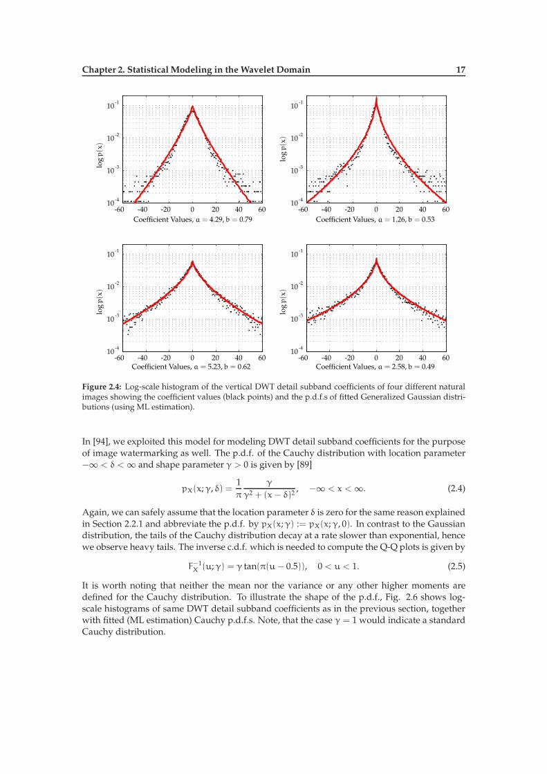
Figure 2.4: Log-scale histogram of the vertical DWT detail subband coefficients of four different naturalimages showing the coefficient values (black points) and the p.d.f.s of fitted Generalized Gaussian distri-butions (using ML estimation).
In [94], we exploited this model for modeling DWT detail subband coefficients for the purposeof image watermarking as well. The p.d.f. of the Cauchy distribution with location parameter−∞ < δ < ∞ and shape parameter γ > 0 is given by [89]
pX(x;γ, δ) =1π
γ
γ2 + (x− δ)2, −∞ < x < ∞. (2.4)
Again, we can safely assume that the location parameter δ is zero for the same reason explainedin Section 2.2.1 and abbreviate the p.d.f. by pX(x;γ) := pX(x;γ, 0). In contrast to the Gaussiandistribution, the tails of the Cauchy distribution decay at a rate slower than exponential, hencewe observe heavy tails. The inverse c.d.f. which is needed to compute the Q-Q plots is given by
F−1X (u;γ) = γ tan(π(u− 0.5)), 0 < u < 1. (2.5)
It is worth noting that neither the mean nor the variance or any other higher moments aredefined for the Cauchy distribution. To illustrate the shape of the p.d.f., Fig. 2.6 shows log-scale histograms of same DWT detail subband coefficients as in the previous section, togetherwith fitted (ML estimation) Cauchy p.d.f.s. Note, that the case γ = 1 would indicate a standardCauchy distribution.

Chapter 2. Statistical Modeling in the Wavelet Domain 18
-50 0 50
0.500
F(b)=
pQuantile-Quantile Plot
-50 0 50
0.003
0.500
0.997
F(b)=
p
Quantile-Quantile Plot
-100 -50 0 50 100
0.004
0.500
0.996
F(b)=
p
Quantile-Quantile Plot
-100 0 100
0.009
0.500
0.991F(b)=
p
Quantile-Quantile Plot
Φ(p) = b Φ(p) = b
Φ(p) = bΦ(p) = b
Figure 2.5: Exemplary Q-Q plots to visualize the GoF of the Generalized Gaussian distribution for theDWT transform coefficients of the vertical detail subband of four natural images (at DWT level two).
Regarding the estimation of the shape parameter γ from an i.i.d. sample x1, . . . , xN, wecan either rely on sample quantile estimation, direct ML estimation or the estimation approachproposed by Tsihrintzis & Nikias [176] for Symmetric α Stable (SαS) distributions [138]. Thelast approach is particularly interesting, since the Cauchy distribution is a special case of anSαS distribution for α = 1 and the estimate of γ can be computed with linear effort, i.e. O(N).Given the estimation setup of our problem, i.e. δ = 0 and α = 1, the shape estimator presentedin [176] is
γ =
[
1N
∑Ni=1 |xi|
p
C(p, 1)
]1/p
with C(p, 1) =1
cos(
π2 p) (2.6)
for 0 < p < 1/2. The parameter p denotes the order of the fractional moment and can bechosen arbitrarily according to [176]. As it is pointed out by the authors, the choice p ≈ 1/3 isreasonable and has shown good performance. Estimation based on the sample quantiles andML estimation is given in [89]. The sample quantiles estimator is γ = 0.5(xq−x1−q) tan[π(1−q)]
where xq denotes the q-th sample quantile (0.5 < q < 1) and the ML estimate of γ is defined as

Chapter 2. Statistical Modeling in the Wavelet Domain 19
-60 -40 -20 0 20 40 6010
-4
10-3
10-2
10-1
Coefficient Values, γ = 3.92
log
p(x
)
-60 -40 -20 0 20 40 6010
-4
10-3
10-2
10-1
Coefficient Values, γ = 2.79
log
p(x
)
-60 -40 -20 0 20 40 6010
-4
10-3
10-2
10-1
Coefficient Values, γ = 7.38
log
p(x
)
-60 -40 -20 0 20 40 6010
-4
10-3
10-2
10-1
Coefficient Values, γ = 7.10
log
p(x
)
Figure 2.6: Log-scale histogram of DWT coefficients from the vertical detail subband of four differentnatural images, showing the coefficient values (black points) and the p.d.f.s of fitted Cauchy distributions(using ML estimation).
the solution to1N
N∑
i=1
21 + (xi/γ)2
− 1 = 0. (2.7)
This equation has to be solved numerically, e.g. using the Newton-Raphson algorithm. Theupdate steps can easily be derived [94]: first, we define the left-hand side of Eq. (2.7) as g(γ)
and then deduce
g(γ)′ :=∂
∂γg(γ) =
4γN
N∑
i=1
x2i(γ2 + x2i)
2. (2.8)
The update step follows as γk+1 = γk −g(γk)/g ′(γk). A possible starting value γ1 is the samplequantile estimate for example. We illustrate the visual GoF by providing a series of Q-Q plotsin Fig. 2.7 for the same subband coefficients we used in the previous section. The plots lookalmost equal to the ones shown in Fig. 2.5, again showing slight deviations in the tail regions.However, since the Q-Q plot just provides a first visual impression of the GoF, we conduct Chi-Square GoF tests on the transform coefficients of a collection of DWT decomposed test imagesin Section 2.2.4.

Chapter 2. Statistical Modeling in the Wavelet Domain 20
-50 0 50
0.002
0.500
0.998
F(b)=
pQuantile-Quantile Plot
-50 0 50
0.500
F(b)=
p
Quantile-Quantile Plot
-100 -50 0 50 100
0.002
0.500
0.998
F(b)=
p
Quantile-Quantile Plot
-100 0 100
0.002
0.500
0.998
F(b)=
p
Quantile-Quantile Plot
Φ(p) = b Φ(p) = b
Φ(p) = bΦ(p) = b
Figure 2.7: Exemplary Q-Q plots to visualize the GoF of the Cauchy distribution for the DWT transformcoefficients of the vertical subband of four natural images.
2.2.3 Multivariate Power Exponential Distribution
Generally speaking, the Multivariate Power Exponential (MPE) distribution is a special case ofKotz-type distribution [132] and can be considered as a multivariate extension of the GGD [58].Verdoolaege et al. [188] first employed this distribution as a statistical model to capture thedependencies of DWT detail subband coefficients across different color channels. In [95], weused the MPE for color image watermarking (see Section 5.3). To illustrate that it is reasonableto use a multivariate model to capture dependencies among subband coefficients of differentcolor channels, Fig. 2.8 shows two exemplary Chi-plots for two subband combinations of thetest image Lena. In case of independence, the points are supposed to lie in the central (shaded)region of the plot. Apparently, there is a quite strong dependency between the coefficientswhich is further confirmed by looking at the numbers for the linear correlation coefficient r,Spearman’s ρ and Kendall’s τ.
In consideration of the non-Gaussian nature of the DWT transform coefficients, the MPEmodel seems to be a good candidate to take the strong association structure into account. The

Chapter 2. Statistical Modeling in the Wavelet Domain 21
λ
χ
-0.5 0 0.5
0
0.2
0.4
0.6
0.8
1
1.2
λ
-0.5 0 0.5
0
0.2
0.4
0.6
0.8
1
χ
r = 0.96, ρ = 0.95, τ = 0.83 r = 0.86, ρ = 0.85, τ = 0.69
HL Subband (Red vs. Green) HL Subband (Red vs. Blue)
Figure 2.8: Exemplary Chi-plots of vertical DWT detail subband (level three of Lena) coefficients extractedfrom the red-green (left) and red-blue (right) color channel combination to illustrate the association amongtransform coefficients of equal subbands but different color channels.
-3-2
-10
12
3
-3-2
-10
12
3
0.005
0.01
0.015
0.02
x
y
p(x
;0,β
,Σ)
Figure 2.9: Exemplary p.d.f. of a MPE distribution.
p.d.f. of a n-variate MPE distribution is given by [58]
pX(x;µ,Σ,β) =nΓ(
n2
)
πn2 Γ(
1 + n2β
)
21+n2β
|Σ|−1/2 exp
−12
[(
x − µ)T Σ−1(x − µ)]β
(2.9)
with x ∈ Rn and parametersβ > 0 (shape), µ ∈ Rn (location) andΣ (positive definite symmetricn × n matrix). The p.d.f. of an exemplary bivariate MPE distribution with µ = 0, β = 0.4 andΣ =
(
1 0.60.6 1
)
is shown in Fig. 2.9.Since we only have three color channels, i.e. n = 3, and we can safely assume a zero location
vector, we have to estimate a 3 × 3 matrix Σ and the shape parameter β. Gomez et al. [58]
Chapter 2. Statistical Modeling in the Wavelet Domain 22
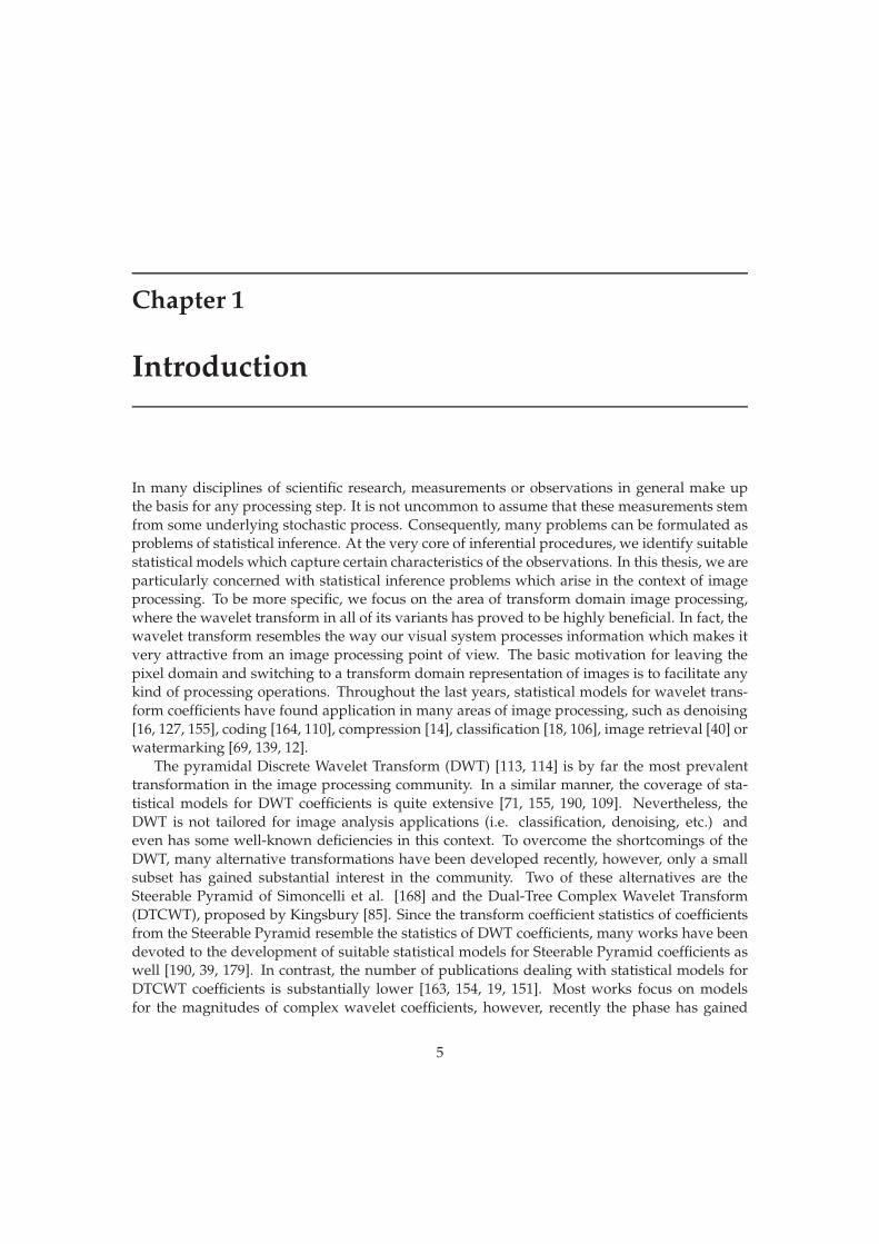
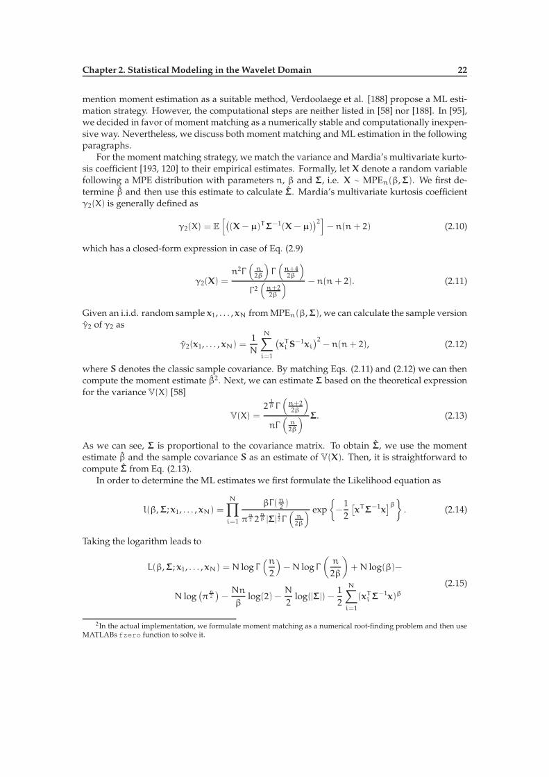
mention moment estimation as a suitable method, Verdoolaege et al. [188] propose a ML esti-mation strategy. However, the computational steps are neither listed in [58] nor [188]. In [95],we decided in favor of moment matching as a numerically stable and computationally inexpen-sive way. Nevertheless, we discuss both moment matching and ML estimation in the followingparagraphs.
For the moment matching strategy, we match the variance and Mardia’s multivariate kurto-sis coefficient [193, 120] to their empirical estimates. Formally, let X denote a random variablefollowing a MPE distribution with parameters n, β and Σ, i.e. X ∼ MPEn(β,Σ). We first de-termine β and then use this estimate to calculate Σ. Mardia’s multivariate kurtosis coefficientγ2(X) is generally defined as
γ2(X) = E
[
(
(X − µ)T Σ−1(X − µ))2]
− n(n + 2) (2.10)
which has a closed-form expression in case of Eq. (2.9)
γ2(X) =n2Γ
(
n2β
)
Γ(
n+42β
)
Γ 2(
n+22β
) − n(n + 2). (2.11)
Given an i.i.d. random sample x1, . . . , xN fromMPEn(β,Σ), we can calculate the sample versionγ2 of γ2 as
γ2(x1, . . . , xN) =1N
N∑
i=1
(
xTi S
−1xi
)2− n(n + 2), (2.12)
where S denotes the classic sample covariance. By matching Eqs. (2.11) and (2.12) we can thencompute the moment estimate β2. Next, we can estimate Σ based on the theoretical expressionfor the variance V(X) [58]
V(X) =2
1β Γ(
n+22β
)
nΓ(
n2β
) Σ. (2.13)
As we can see, Σ is proportional to the covariance matrix. To obtain Σ, we use the momentestimate β and the sample covariance S as an estimate of V(X). Then, it is straightforward tocompute Σ from Eq. (2.13).
In order to determine the ML estimates we first formulate the Likelihood equation as
l(β,Σ; x1, . . . , xN) =
N∏
i=1
βΓ(n2 )
πn2 2
nβ |Σ|
12 Γ(
n2β
) exp
−12
[
xTΣ−1x]β
. (2.14)
Taking the logarithm leads to
L(β,Σ; x1, . . . , xN) = N log Γ(n
2
)
−N log Γ(
n
2β
)
+N log(β)−
N log(
πn2)
−Nn
βlog(2) −
N
2log(|Σ|) −
12
N∑
i=1
(xTi Σ−1x)β
(2.15)
2In the actual implementation, we formulate moment matching as a numerical root-finding problem and then useMATLABs fzero function to solve it.

Chapter 2. Statistical Modeling in the Wavelet Domain 23
which can now be used to calculate the partial derivatives w.r.t. β and Σ using basic algebraand matrix calculus, i.e.
∂
∂βL(β,Σ; x1, . . . , xN) =
1β
[
N+Nn
β
(
log(2) +ψ
(
n
2β
))]
−
12
N∑
i=1
log(xTi Σ−1x)(xT
i Σ−1x)β
(2.16)
and∂
∂ΣL(β,Σ; x1, . . . , xN) = −
N
2Σ−1 +
β
2
N∑
i=1
(xTi Σ−1x)β−1Σ−1xix
Ti Σ−1. (2.17)
The solutions β and Σ to both equations are the ML estimates. It is worth noting, that aftersetting the right-hand side of Eq. (2.17) to zero and performing some straightforward manipu-lations (i.e. multiplying two times by Σ) we obtain
Σ =β
N
N∑
i=1
xixTi
(
xTi Σ−1xi
)β−1(2.18)
which allows to employ a fix-point iteration directly (e.g. Picard Iteration aka successive sub-stitution). Since it is hard to prove that Eq. (2.18) actually is a contraction – which wouldguarantee convergence to the fixpoint – we follow an alternative technique to obtain the esti-mates. We directly try to minimize the negative Log-Likelihood, i.e. −L(β,Σ; x1, . . . , xN), usinga gradient descent approach. This is an optimization problem with non-linear constraints, sincewe have to satisfy the requirements that Σ must be positive definite and symmetric and β > 0.We already have the derivatives of the log-likelihood function w.r.t. β and Σ, see Eq. (2.16)and (2.17). To take care of the positive definiteness criteria, we use the Sylvester criterion [126]which requires that all leading principal minors of Σ are positive. This is a necessary and suffi-cient condition to guarantee positive definiteness. Eventually, we have (n+ 1)/2− 1 unknownsto solve3 (since Σ is symmetric).
2.2.4 Quantifying the Goodness-of-Fit
In order to quantify the GoF of the presented GGD and Cauchy model, we conduct a seriesof Chi-Square GoF tests using the images of the UCID database. Each RGB channel is decom-posed separately by a three-scale DWT and the test statistic is computed using the transformcoefficients of each detail subband. In contrast to the Chi-Square tests we conducted in [101],we slightly modify the test setup here to account for different sample sizes on each decompo-sition level. The problem with the test in [101] can be formulated as follows: first, the typeof GoF test setup we use here can be termed an Accept-Support testing setup. This means thatthe null-hypothesis represents what we actually believe (i.e. the observations stem from thedistribution we assume). Second, we know that increasing the sample size likewise increasesthe power of a hypothesis test. Hence, if the sample size is too large, we will inevitably decideagainst the null-hypothesis even in cases when the model represents a good fit to the data. Thishappens because even minor deviations from the null-hypothesis are rigorously penalized in
3In the actual implementation of this estimation procedures, the non-linear optimization problem with non-linearconstraints is solved by means of MATLAB’s fminbnd routine.

Chapter 2. Statistical Modeling in the Wavelet Domain 24
Database LevelModel
GGD Cauchy
UCID1 36.64 62.042 35.14 62.553 34.73 71.62
Stex1 0.82 41.632 1.23 43.913 2.34 32.79
Vistex (small)1 0.57 44.642 0.94 43.963 2.34 34.74
Vistex (full)1 0.87 42.682 1.20 36.333 2.26 28.60
Outex1 1.76 70.952 0.60 55.243 0.76 32.06
Table 2.1: Percentage of rejected null-hypotheses of Chi-Square GoF tests (at 5% significance), averagedover all subbands of a DWT decomposition level.
case of large sample size. Due to subsampling, the number of DWT coefficients on successivescales differs by a factor of four. Hence, we have 16 times more coefficients on level one as wehave on level three for example. The aforementioned sample size effect on the test power wouldtherefore inevitably lead to more rejections of the null-hypothesis at lower decomposition lev-els. In order to deal with that problem, we modify the GoF setup such that we limit the samplesize to N samples, randomly selected from each subband. In detail, we use uniform samplingwithout replacement. The percentage of rejected null-hypotheses on each DWT decompositionlevel for the GGD and Cauchymodel is listed in Table 2.1 usingN = 500. As expected, the GGDis a quite good model for the coefficients of DWT decomposed images. The Cauchy distributionon the other hand leads to higher rejection rates, however, we emphasize that this model is onlysupposed to be a better approximation to the coefficients than the Gaussian model. In contrastto [101], we further notice that the rejection rates are now rather stable over the decompositionlevels.
Testing the GoF of the MPE Distribution
To the best of our knowledge, there exists no published GoF test for the MPE distribution,although Gomez et al. [58] sketch a possible test strategy. We first discuss this idea and thenintroduce a novel GoF test which is based on a generic test for multivariate normality. Theapproach proposed by Gomez et al. is a three-stage strategy which relies on the stochasticrepresentation of the MPE distribution. Unfortunately, no clear description of how to performthe three stages is given by the authors. In the following, we discuss a possible implementation

Chapter 2. Statistical Modeling in the Wavelet Domain 25
of the test. We know that in case X ∼ MPEn(x;β,Σ), then
X ∼ rATu (2.19)
where r is a realization of the random variable R ∼ fR(r;β) with p.d.f.
fR(r;β) =n
Γ(
1 + n2β
)
2n2β
rn−1 exp
−12r2β
1(0,∞)(r). (2.20)
The vector u ∈ Rn is uniformly distributed on the unit sphere and A is a lower triangularmatrix such that Σ = AT A. Based on this stochastic representation of the MPE distribution andthe moments of R [58], the first step of the GoF procedure is to test whether
Z =(
(x − µ)T Σ−1(x − µ))β
(2.21)
follows a Gamma distribution [89] with shape parameter 2 and scale parameter n/2β. This caneasily be accomplished by means of a Chi-Square GoF test. In the second step, we have to testwhether
u =Σ
− 12 x
∥
∥
∥
∥
Σ− 1
2 x)
∥
∥
∥
∥
(2.22)
is uniformly distributed on the unit sphere in Rn (in fact, it is the unit ball in the n-dimensionalEuclidean space). We perform this task bymeans of a Rayleigh test for uniformity on the sphere,originally proposed by Mardia and Rupp [121]. In the last step, we test if the random variable Ris independent of u. For that purpose, we employ a very recently proposed test by Gretton et al.[60]. Probably the most crucial step is the fusion of the three test results. We choose the ratherstrict strategy to reject the overall null-hypothesis, in case one test shows evidence against itsnull-hypothesis. At the end of this section, we will assess the size and power of this test. To thebest of our knowledge, no such study has been conducted so far.
As a second, novel alternative to assess the GoF of the MPE distribution, we propose amodification of the GoF test for a multivariate normality proposed by Smith & Jain [170]. Thecomponents of the test procedure are outlined in Fig. 2.10. The left part shows the Monte-Carlo variant of the test which is based on an estimate of the p-value. The right part shows thesecond variant which relies on the asymptotic distribution of the test statistic under the null-hypothesis. In [170], the null-hypothesis is that the observations x1, . . . , xN are drawn from amultivariate Gaussian distribution N(µ,Σ) with parameter vector Θ = [µ Σ]. Consequently,the null-hypothesis of our MPE GoF test is that the data is drawn from a MPE distributionMPEn(β,Σ) with parametersβ andΣ, henceΘ = [β Σ]. According to Fig. 2.10, the critical partsof the GoF test are the estimation part, the sampling part and the computation of a suitable teststatistic. Estimation and sampling in the multivariate Gaussian case is straightforward and awell covered topic in literature. Estimation of the MPE parameters has already been discussedin Section 2.2.3. Hence, the remaining parts are the sampling step in case of theMPE distributionand the definition of a test statistic. Both topics are covered next:
Sampling from a MPE distribution We can rely on the stochastic representation of the MPEdistribution, given in Eq. (2.19). For our purpose, we assume µ = 0. In order to gener-ate a random sample from a MPE distribution MPEn(β,Σ) we have to draw a randomsample u1, . . . ,uN from a uniform distribution on the n-dimensional unit sphere first. We

Chapter 2. Statistical Modeling in the Wavelet Domain 26
estimate
sample
sample
estimate
sample
statistic
statistic
Ti
W
x1, . . . , xN
x∗1 , . . . , x∗
N
y∗
1 , . . . , y∗
N
Θ∗
Θ
y1, . . . , yN
T∗
Wti
mes
(a) "Monte-Carlo" Test
estimate
T∗∼ N(µ, σ)
sample
statistic
x1, . . . , xN
y1, . . . , yN
Θ
(b) "Normal" Test
Figure 2.10: Outline of the generic GoF test setup proposed by Smith & Jain [170], originally intended totest for multivariate normality.
then perform a Cholesky decomposition of Σ to obtain AT and generate another randomsample r1, . . . , rN from the distribution given by the p.d.f. in Eq. (2.20). Eventually, weuse
∀i, 0 < i < N : xi = riATui (2.23)
to generate a MPE random sample x1, . . . , xN of sizeN. To obtain u1, . . . ,uN, several waysare possible. We choose the simple strategy of generating a random vector ui from amultivariate Gaussian distribution N(0, 1) and then normalize each element of the vec-tor by (
∑j u
2ij)
1/2. Due to the radial symmetry of the multivariate Gaussian distribution,this gives a random vector which is uniformly distributed on the unit sphere in the n-dimensional Euclidean space. The process of generating the random sample r1, . . . , rN isslightly more involved. In order to use the classic inversion method, we first need to de-termine the quantile function F−1
R (i.e. the inverse c.d.f.) corresponding to the p.d.f. givenin Eq. (2.20). First, we derive the c.d.f. as
FR(y;β) =
∫y
0fR(x;β)dx = 1 −
Γ(
n2β , y2β
2
)
Γ(
n2β
) . (2.24)
Inverting the c.d.f. gives the desired result
F−1R (u;β) = 2
12β
[
P−1u
(
n
2β, 1 − u
)] 12β
(2.25)
where Pu(a, x) is defined as in Eq. (2.3). We can then generate ri by using ri = F−1R (ui;β)
with ui ∼ U(0, 1).
Defining a suitable test statistic In [170], Smith & Jain propose to test for multivariate normal-ity by first computing the Euclidean Minimum Spanning Tree (EMST) of the pooled sample
∀i, 0 < i 6 2N : zi =
xi, 0 < i 6 N
yi, N < i 6 2N(2.26)

Chapter 2. Statistical Modeling in the Wavelet Domain 27
(a) H 6= G,T = 6 (b) H = G,T = 2
Figure 2.11: Illustration of the two-sample hypothesis test proposed by Henze [68] based on thenumber of nearest neighbor coincidences. In case the samples stem from the same population (i.e.H = G), we expect the test statistic T to be low, while in case the samples stem from differentpopulations (i.eH 6= G) we expect the test statistic to be high.
The sample x1, . . . , xN denotes the collection of original observations, whereas the sam-ple yi, . . . ,yN is drawn from a multivariate Gaussian distribution with parameters fittedon the basis of xi. The test statistic T is defined as the number of edges connecting ver-tices from different samples. This idea was first introduced by Friedman & Rafsky [49] inthe field of multivariate two-sample hypothesis testing, where the objective is to quantifywhether two samples stem from the same population without making any assumptionsabout the distribution family. In the same context, a similar strategy is suggested byHenze[68], based on the computation of the number of nearest neighbor coincidences. A graph-ical visualization of the NN coincidences idea is shown in Fig. 2.11, where H signifies thedistribution of the first sample (marked as blue squares) and G signifies the distributionof the second sample (marked as red discs). The value of the test statistic when we onlyconsider two elements of each sample is given as T . The basic idea of the EMST and NNcoincidences approach is the same: given that the null-hypothesis is true, we (i) expectthat the number of EMST edges connecting vertices from different samples to be high and(ii) the number of nearest neighbor coincidences to be low.
When using the EMST approach for testing multivariate normality as in [170], we conse-quently expect high values of T in case the observations xi actually follow a multivariateGaussian distribution and vice versa. From Friedman & Rafsky [49], we know that in casethe null-hypothesis is true, the test statistic T follows a Gaussian distribution with meanµ and standard deviation σ. Hence, it is straightforward to compute a p-value and rejectthe null-hypothesis if the p-value is less than the fixed significance level α. However, itis worth noting that the sampling procedure to generate yi introduces bias, because sam-pling is based on the distribution parameters fitted on the basis of xi. Since the EMSTand NN coincidences approach rely on the assumption of independent random samples,the resulting GoF tests will inevitably loose power. A reasonable way to circumvent theindependency problem is to estimate the critical region of the test using aMonte-Carlo ap-proach, illustrated in Fig. 2.10a. The iteration in the right branch of Fig. 2.10a is repeatedW times and the p-value estimate is finally obtained by
p =#Ti > T∗ + 0.5
W + 1. (2.27)
To construct a GoF test for the MPE distribution similar to the one of Smith & Jain, we use(i) the gradient decent approach of minimizing the negative Log-Likelihood to estimate

Chapter 2. Statistical Modeling in the Wavelet Domain 28
the MPE parameters, (ii) the MPE sampling procedure outlined above and (iii) the NN co-incidences approach of [68] to obtain a test statistic T . To provide full detail, let z1, . . . , zM
denote the pooled sample (i.e. M := 2N); further, let m denote a function returning thesample membership of zi and letNNi(r) denote the r-th nearest neighbor of zi (in the Eu-clidean norm). Then, the formal description of the NN coincidences test statistic is givenby
Tk,M =1Mk
M∑
i=1
k∑
r=1
1i(r) (2.28)
where 1i(r) denotes the indicator function of the event that m(zi) = m(NNi(r)). Ac-cording to Schilling [160], we have the asymptotic (i.e. M → ∞) result that in case thenull-hypothesis (denoted by H0) is true, the term
√Mk
(
Tk,n − µTk,M|H0
σTk,M|H0
)
∼ N(0, 1) (2.29)
follows a standard normal distribution with
µTk,M|H0 = λ21 + λ22, σ2Tk,M|H0= λ1λ2 + 4λ21λ
22
[
1 −
(
2kk
)
2−2k]
(2.30)
and λi = N/M (i.e. in our case λ1 = λ2 = 0.5). By using Eqs. (2.29) and (2.30), thep-value can be calculated by determining P(T∗ > T |H0), i.e. the probability of obtaininga test statistic at least as extreme as T∗. Adhering to the terminology of Smith & Jain,we denote the test variant based on the Monte-Carlo p-value estimation approach as the"Monte-Carlo" test and the second variant, based on the asymptotic normality of T , as the"Normal" test.
In order to assess the quality of the proposedGoF test and the test suggested by Gomez et al.,we conduct a study on the size, i.e. the test’s probability of falsely rejecting the null-hypothesis,and power of the test. Regarding the methodology, both size and power are evaluated bymeansof a Monte-Carlo strategy with M = 500 iterations for the case n = 3 (i.e. three-dimensionalobservations).
Size Study In each Monte-Carlo iteration, we sample N points from a MPE3(0.5, I) distribu-tion and determine the percentage of rejected null-hypotheses. We let the sample size Nbe 200, 400 and 800. Since we do not obtain an overall p-value in case of the GoF testof Gomez et al., we have to decide when to reject the null-hypothesis based on the out-comes of the three stages. As mentioned before, we choose the strict way of rejecting thenull-hypothesis in case just one stage rejects its own null-hypothesis. Formally, given thatHi, i = 1, 2, 3 denotes the outcome of stage i (i.e. Hi ∈ 0, 1), we reject the null-hypothesisif
∑iHi > 0. Regarding the “Monte-Carlo” variant of our proposed GoF test, we set the
number of iterations W to 1000. Tables 2.2 and 2.3 list the estimated significance level αfor different sample sizes. For the Gomez et al. GoF test, we observe that the estimatedpercentage of rejections α is above the desired significance level α in all cases. Regardingthe two variants of our proposed GoF approach, we can see that the “Monte-Carlo” test isquite conservative, i.e. the percentage of false positives is always below the fixed signif-icance level. However, in case of the "Normal" test, the situation is different. Except forN = 400, the rejection rates are always slightly above the desired level.

Chapter 2. Statistical Modeling in the Wavelet Domain 29
Significance Sample SizeN
∑iHi > 0
α
α = 0.01200 0.030400 0.028800 0.014
α = 0.05200 0.084400 0.118800 0.108
α = 0.10200 0.194400 0.212800 0.196
Table 2.2: Rejection rates for the three-stage GoF test sketched by Gomez et al. in [58] for variouslevels of α and various sample sizesN.
Significance Sample SizeN“Monte-Carlo” "Normal"
α α
α = 0.01200 0.002 0.022400 0.001 0.002800 0.001 0.018
α = 0.05200 0.022 0.063400 0.012 0.014800 0.053 0.069
α = 0.10200 0.044 0.132400 0.026 0.048800 0.084 0.1520
Table 2.3: Rejection rates for the two variants of the proposed MPE GoF test for various levels of αand different sample sizesN.
Power Study To assess the power of the GoF tests, we sample from a two-component mixtureof MPE distributions. Given that p(x;βi,Σi) := MPE3(x;βi,Σi), the mixture p.d.f. isgiven by
p(x;π1,π2,β1,β2,Σ1,Σ2) =
2∑
i=1
πip(x;βi,Σi) with∑
i
πi = 1. (2.31)
We start from an equal parameters β1 = β2 = 0.5,Σ1 = Σ2 and then move the shapeparameter β2 of the second mixture component away from the original choice, as illus-trated in Fig. 2.12. The component weights are set to π1 = π2 = 0.5. For each param-eter setting along the line we perform M Monte-Carlo iterations for each sample sizeN ∈ 200, 400, 800 and determine the number of rejected null-hypotheses. Figures 2.13and 2.14 show the corresponding power plots, where the x-axis shows the shape param-eter value of β2 and the y-axis shows the percentage of rejected null-hypotheses. In case

Chapter 2. Statistical Modeling in the Wavelet Domain 30
β1 = 0.5, β2 = 0.5 β1 = 0.5, β2 = 3
β2 = 0.6 β2 = 2.9
Figure 2.12: Illustration of the power study procedure for scale alternatives. The starting model is amixture of two MPE distributions with β1 = β2 = 0.5, Σ1 = Σ2 = I and equal weights π1 = π2 = 0.5.As we progress from left to right, the shape parameter β2 of the second mixture component isincreased by a stepsize of 0.1.
0.5 1 1.5 2 2.5 30
0.2
0.4
0.6
0.8
1
Po
wer
N=200
N=500
N=800
0.5 1 1.5 2 2.5 30
0.2
0.4
0.6
0.8
1
Po
wer
N=200
N=500
N=800
β2 β2
Rejection Criterion:∑
iHi > 1Rejection Criterion:
∑iHi > 0
Figure 2.13: Power vs. β2 for two choices of how to combine the three-stages of the Gomez et al.GoF test. The plot on the left-hand side shows the results of the rejection criterion we select for ourtests.
of the GoF test of Gomez et al. (see Fig. 2.13), we observe that our fusion strategy ofthe three stages leads to reasonable power, even at moderate sample size, i.e. N = 200.For comparative reasons, we additionally show a power plot for the case of requiringevidence against the null-hypothesis in at least two of the three stages. In this case, thetest exhibits almost no power at all and renders this setting useless. Regarding the twovariants of our proposed GoF test, both exhibit reasonable power with the "Normal" testshowing high power even at moderate sample size. The higher power can be explainedby referring to Table 2.3, where the "Normal" test exhibits less conservative behavior thanthe "Monte-Carlo" test.
After completing the size and power study, we finally turn to the actual application of theGoF test. We apply the test to the DWT detail subband coefficients of our database images. Toobtain the same power for eachDWTdecomposition level, we uniformly sample 500 coefficientsfrom each subband and set the significance level to α = 0.05. We choose the "Normal" GoF testvariant in all cases. In addition to the estimation of both MPE parameters, we test against thefix choice of β = 1, i.e. multivariate Gaussian, for comparative reasons. The rejection rates arelisted in Table 2.4. Apparently, the MPE distribution is a quite good model for textured imagesand slightly worse for natural images. However, compared to the GoF results for β = 1, theMPE distribution is definitely the more suitable statistical model to capture the non-Gaussiannature of the coefficients.

Chapter 2. Statistical Modeling in the Wavelet Domain 31
0.5 1 1.5 2 2.5 30
0.2
0.4
0.6
0.8
1
β2
Po
wer
N=200
N=500
N=800
0.5 1 1.5 2 2.5 30
0.2
0.4
0.6
0.8
1
β2
Po
wer
”Normal” Test
N=200
N=500
N=800
”Monte-Carlo” Test
Figure 2.14: Power vs. β2 for the two variants of the proposed GoF test, i.e. using either the Monte-Carlo approach to approximate the critical region or the Normal approximation of the test statistic.
ModelDatabases
Stex Vistex (full) Outex UCID
MPE 25.09 35.13 11.15 56.18Gaussian (β = 1) 57.13 73.19 39.66 98.97
Table 2.4: Rejection rates of the MPE "Normal" GoF test at 5% significance for several image databases.The second row lists the GoF test results of the same test when we fix the shape parameter to β = 1, i.e.multivariate Gaussian.
2.3 Complex Wavelet Transform SubbandModels
Since two major parts of this thesis, namely Chapters 3 and 4 are concernedwith image analysisapplications, we select the Dual-Tree Complex Wavelet transform [85, 86] (DTCWT) as a secondwavelet transform variant due to its advantages over the DWT. In particular, the DTCWT over-comes two shortcomings of the DWT: lack of shift-invariance and lack of directional selectivity,as it is vividly illustrated and explained in [86] or [162]. These shortcomings are especially rele-vant for image analysis purposes. Lack of shift-invariance implies that singularities at differentlocations in an image lead to different representations in the wavelet domain (i.e. different coef-ficients). Hence, wavelet coefficients representing an edge along an object contour for example,are not necessarily large across all scales which causes ringing artifacts when reconstruction isperformed using only a subset of the coefficients. Of course, the perfect reconstruction propertyguarantees that all artifacts are canceled when computing the reconstruction using all coeffi-cients. The technical reason for the shift-dependency problem is that the wavelet and scalingfilters which are used to implement the DWT have finite support and the coefficients are down-sampled by two after each decomposition stage. As a matter of fact, shift-dependency is asevere deficiency in the context of image analysis. The second shortcoming – lack of direction-ally selectivity – is related to the fact that the filters of the DWT are real functions and are thussupported on both sides of the frequency axis. Since the 2-D DWT is usually implemented by
Chapter 2. Statistical Modeling in the Wavelet Domain 32
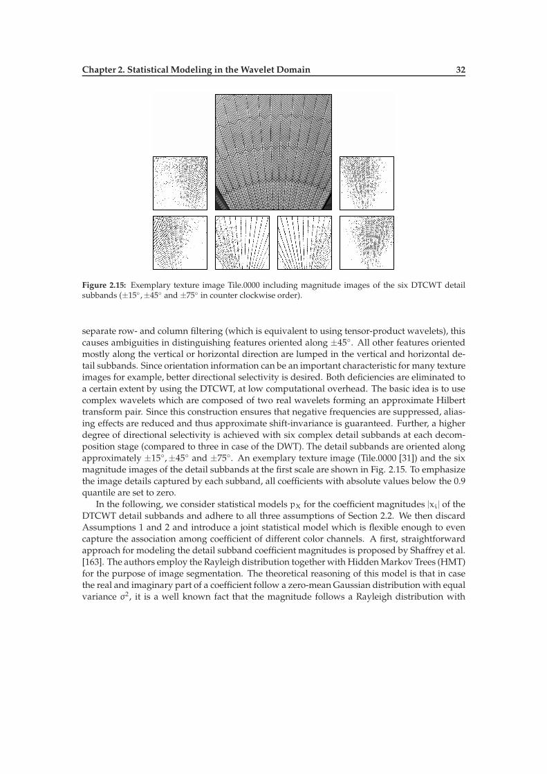
Figure 2.15: Exemplary texture image Tile.0000 including magnitude images of the six DTCWT detailsubbands (±15,±45 and ±75 in counter clockwise order).
separate row- and column filtering (which is equivalent to using tensor-product wavelets), thiscauses ambiguities in distinguishing features oriented along ±45. All other features orientedmostly along the vertical or horizontal direction are lumped in the vertical and horizontal de-tail subbands. Since orientation information can be an important characteristic for many textureimages for example, better directional selectivity is desired. Both deficiencies are eliminated toa certain extent by using the DTCWT, at low computational overhead. The basic idea is to usecomplex wavelets which are composed of two real wavelets forming an approximate Hilberttransform pair. Since this construction ensures that negative frequencies are suppressed, alias-ing effects are reduced and thus approximate shift-invariance is guaranteed. Further, a higherdegree of directional selectivity is achieved with six complex detail subbands at each decom-position stage (compared to three in case of the DWT). The detail subbands are oriented alongapproximately ±15,±45 and ±75. An exemplary texture image (Tile.0000 [31]) and the sixmagnitude images of the detail subbands at the first scale are shown in Fig. 2.15. To emphasizethe image details captured by each subband, all coefficients with absolute values below the 0.9quantile are set to zero.
In the following, we consider statistical models pX for the coefficient magnitudes |xi| of theDTCWT detail subbands and adhere to all three assumptions of Section 2.2. We then discardAssumptions 1 and 2 and introduce a joint statistical model which is flexible enough to evencapture the association among coefficient of different color channels. A first, straightforwardapproach for modeling the detail subband coefficient magnitudes is proposed by Shaffrey et al.[163]. The authors employ the Rayleigh distribution together with HiddenMarkov Trees (HMT)for the purpose of image segmentation. The theoretical reasoning of this model is that in casethe real and imaginary part of a coefficient follow a zero-mean Gaussian distribution with equalvariance σ2, it is a well known fact that the magnitude follows a Rayleigh distribution with

Chapter 2. Statistical Modeling in the Wavelet Domain 33
shape parameter β := σ. The p.d.f. of a Rayleigh distribution is given by [89]
pX(x;β) =x
β2 exp(
−x2
2β2
)
, 0 < x < ∞ (2.32)
with β > 0. In Fig. 2.16 we illustrate the shape of the Rayleigh p.d.f. and the characteristiccoefficient histograms which can be observed in case of texture images. ML parameter estima-tion of β has a closed-form solution which can be found in [89]. In a very recent work, Rahmanet al. [151] studied the statistics of DTCWT detail subband coefficients restricted to the decom-position of Gaussian distributed signals. The authors show that the real and imaginary partcan actually be modeled by zero-mean Gaussian distributions for decomposition levels greaterthan one and hence allow to employ the Rayleigh model for the magnitudes. On the first level,however, they propose to use a Generalized Gamma distribution [174] instead. The reason forswitching the statistical models is that on the first level of the DTCWT it is necessary to use dif-ferent filter sets (e.g., see [162]) which violate the Hilbert transform property. As a result, the realand imaginary parts no longer show equal variances and hence prevent to employ the Rayleighdistribution to model the magnitudes. Although the results presented in [151] are theoreticallyinteresting, they lack practical application, since we rarely observe a Gaussian distributed signalin image processing. The effect of the deviation from Gaussianity is apparent by looking at thebad fit of the Rayleigh model in Fig. 2.16. The idea of using a Generalized Gamma distributionto model the coefficient magnitudes is a good starting point, though. Apparently, candidatemodels are positively skewed distributions (i.e. skewed to the right) which are often used inreliability and life-span modeling [23]. Similar distributions are also employed in modeling theamplitude statistics of Synthetic Aperture Radar (SAR) data (e.g. see [130, 93]). The use of theGeneralized Gamma distribution, however, is not widespread due to the difficulties in param-eter estimation (e.g., see [172]). In the following, we present two reasonable statistical modelswhich are both special cases of the Generalized Gamma distribution, allowing computationallyefficient parameter estimation. Further, we show that the models are flexible enough to capturethe magnitude distributions.
2.3.1 Weibull Distribution
The first model we consider is the two-parameterWeibull distributionwhich includes the Rayleighdistribution as a special case. This model is a reasonable choice since there are more degrees offreedom to adapt to the underlying data. In [98], we exploited the Weibull distribution parame-ters for the purpose of medical image classification and in [101, 61] this model was successfullyemployed in texture image retrieval. The p.d.f. and c.d.f. of a Weibull distribution, as given in[89], are
pX(x;α,β) =α
β
(
x
β
)α−1
exp
−
(
x
β
)α
, 0 < x <∞ (2.33)
and
FX(x;α,β) = 1 − exp
−
(
x
β
)α
(2.34)
with shape parameter α > 0 and scale parameter β > 0. For α = 2 and β =√2β, Eq.
(2.33) reduces to the Rayleigh distribution. The inverse c.d.f. has the closed form expressionF−1(u;α,β) = β[− log(1 − u)]1/α. Regarding parameter estimation of α and β, we discuss bothmoment matching and ML estimation. First, lets assume that we have an i.i.d. random sample

Chapter 2. Statistical Modeling in the Wavelet Domain 34
0 100 200 3000
0.005
0.01
0.015
0.02
0.025
Coefficient Values
p(x
)
0 50 100 150 2000
0.005
0.01
0.015
0.02
0.025
0.03
0.035
Coefficient Values
p(x
)
0 50 100 150 2000
0.005
0.01
0.015
Coefficient Values
p(x
)
0 50 100 150 2000
0.01
0.02
0.03
0.04
0.05
Coefficient Values
p(x
)
Figure 2.16: Exemplary DTCWT coefficient histograms (i.e. |xi|) of the +75 subband on DTCWT leveltwo of four texture images together with fitted Rayleigh p.d.f.s.
x1, . . . , xN drawn from a two-parameter Weibull distribution. According to [89], the MLE of αis the solution to g(α) = 0 with
g(α) :=
N∑
i=1
xαi log(xi) − K
N∑
i=1
xαi −
1α
N∑
i=1
xαi (2.35)
and K := 1N
∑Ni=1 log(xi). In order to solve Eq. (2.35) using Newton-Raphson root finding, we
first determine the first derivative g ′(α) as
g ′(α) :=∂
∂αg(α) =
N∑
i=1
xαi log(xi)
2−
K
(
N∑
i=1
xαi log(xi)
)
+1α2
N∑
i=1
xαi −
1α
N∑
i=1
xαi log(xi).
(2.36)

Chapter 2. Statistical Modeling in the Wavelet Domain 35
The MLE is then obtained by using the update step αn = αn−1 − g(αn−1)/g′(αn−1) for n > 2.
Subsequently, the MLE of β has the explicit expression:
β =
(
1N
N∑
i=1
xαi
)1/α
(2.37)
The starting value α1 is usually computed by moment matching. Unfortunately, even that re-quires a numerical procedure, since the moment parameter estimate α is the solution to [23]
Γ3 − 3Γ2Γ1 + 2Γ 31(
Γ2 − Γ 21)3/2 − a3 = 0, (2.38)
where Γk := Γ(1 + k/α) and
a3 :=1N
∑Ni=1(xi − x)3
[
1N
∑Ni=1(xi − x)2
]3/2 (2.39)
denotes the sample skewness. A first approximation of α to solve Eq. (2.39) can be obtainedfrom a α-versus-a3 lookup-table and linear interpolation. The moment estimate of β is thencomputed by
β =s
(
Γ2 − Γ 21)
12
(2.40)
where s denotes the sample standard deviation and Γk signifies that we use the moment esti-mate α to compute Γ1 and Γ2. Finally, it is worth noting that computational difficulties can arisefor ML estimation in cases where α < 2.2 [23].
We next present an alternative estimation method which is computationally more attractivethan the direct ML estimation approach from above. This estimation strategy is based on thetheoretical result, that if a random variable X follows a Weibull distribution, then the randomvariable Y = log(X) follows an Extreme Value (EV) distribution of type I (i.e. Gumbel distri-bution) [118]. This result can easily be verified by exploiting the fact that the random variabletransformation t(X) is the natural logarithmwhich is monotonically increasing, continuous anddifferentiable. Hence, we have FY(y) = P(Y 6 y) = P(X 6 t−1(x)) = FX(t−1(y)) which in ourcase (i.e. t(x) = log(x) and t−1(x) = exp(x)) leads to
FY(y) = FX(exp(y)) (2.41)
= 1 − exp
−
[
exp(y)
β
]α
(2.42)
= 1 − exp
−
[
expy− µ
σ
]
(2.43)
using the substitution σ := 1/α and µ := log(β) in Eq. (2.43). The last expression in this deriva-tion is the c.d.f. of a Gumbel distribution. Given that we set yi := log(xi), the correspondingp.d.f. follows as
pY(y;µ,σ) =1σexp
(
y− µ
σ
)
exp
− exp(
y− µ
σ
)
, −∞ < y < ∞ (2.44)

Chapter 2. Statistical Modeling in the Wavelet Domain 36
with location parameter 0 < µ < ∞ and scale parameter σ > 0. This extreme-value distributionmight be thought of as a log-Weibull distribution [23]. The MLE of σ requires a numericalsolution to f(σ) = 0 with
f(σ) := y− σ−
∑Ni=1 yi exp
(
−yi
σ
)
∑Ni=1 exp
(
−yi
σ
) (2.45)
where y denotes the sample mean of the observations. Again, to derive the update step of theNewton-Raphson algorithm, we first determine the derivative of f(σ) w.r.t. σ as
f ′(σ) :=∂
∂σf(σ) =
1σ2
N∑
i=1
y2i exp(
−yi
σ
)
+
N∑
i=1
exp(
−yi
σ
)
+1σ
N∑
i=1
yi exp(
−yi
σ
)
− y1σ2
N∑
i=1
yi exp(
−yi
σ
)
(2.46)
which then allows to formulate the update step as σn = σn−1 − f(σn−1)/f′(σn−1) for n > 2. In
contrast to the problematic computation of the starting value α1 in Eq. (2.38) which we obtainedby moment matching, the starting value σ1 can be easily obtained from the explicit expressionsof the moment estimates [23]
σ =1π
√6s ≈ 0.779697s and µ = y− γσ, (2.47)
where γ denotes the Euler-Mascheroni constant, i.e. γ ≈ −0.57. Eventually, we can use themoment estimate of σ to start the Newton-Raphson algorithm and obtain the correspondingML estimate. Inserting the ML estimate of σ into
µ = σ log
(
1N
N∑
i=1
exp(yi
σ
)
)
(2.48)
gives the ML estimate of µ. The only thing left to do is to transform the parameter estimates µand σ back to the estimates α and β of the Weibull distribution. From the substitution we usedin Eq. (2.43) we deduce
α =1σ
and β = exp(µ). (2.49)
To visualize the GoF of the Weibull distribution, Fig. 2.17 shows a set of Q-Q plots for thesame DTCWT detail subband coefficients of Fig. 2.16. As we can see, the points approximatelyfollow the dashed red line which indicates that the Weibull model is a reasonable choice here.
2.3.2 Gamma Distribution
A second, alternative model which also occurs in the literature of reliability and life span mod-eling is the two-parameter Gamma distribution. The Gamma distribution has been proposed asan alternative to the Rayleigh distribution for modeling the magnitudes of Gabor filter outputs[123] for instance. The p.d.f. and c.d.f., as given in [89], are
pX(x;α,β) =β−αxα−1
Γ(α)exp
(
−x
β
)
, x < 0 < ∞ (2.50)

Chapter 2. Statistical Modeling in the Wavelet Domain 37
50 100 1500.002
0.911
0.998
F(b
)=
p
Φ(p) = b
Quantile-Quantile Plot
20 40 60 80 100 1200.002
0.898
0.998
F(b
)=
p
Φ(p) = b
Quantile-Quantile Plot
50 100 1500.002
0.809
0.998
F(b
)=
p
Φ(p) = b
Quantile-Quantile Plot
20 40 60 80 1000.002
0.931
0.998
F(b
)=
p
Φ(p) = b
Quantile-Quantile Plot
Figure 2.17: Exemplary Q-Q plots for GoF of the Weibull distribution.
and
FX(x;α,β) = Pl
(
a,x
β
)
(2.51)
with shape parameter α > 0 and scale parameter β > 0, respectively. The term Pl(a, x) denotesthe regularized (lower) incomplete Gamma function, i.e.
Pl(a, x) =1Γ(a)
∫x
0ta−1 exp(−t)dt. (2.52)
The inverse c.d.f. can be computed by F−1X (u;α,β) = βP−1
l (α, 0,u) which is the numericalsolution for x to the equation u = Pl(α, 0, x/β). In order to estimate the parameters α andβ, we follow the approach presented by Choi & Wette [20]. The authors already provide theNewton-Raphson update step to compute the ML estimate of α as
αn = αn−1 −log(αn−1) −ψ(αn−1) −M
1/αn−1 −ψ′
(αn−1), (2.53)
for n > 2. Here, ψ and ψ ′ denote the Digamma and Trigamma function [1], resp., and M isdefined as
M := log(x) −1N
N∑
i=1
log(xi). (2.54)

Chapter 2. Statistical Modeling in the Wavelet Domain 38
Given the ML estimate of α, the ML estimate of β has the closed-form expression
β =µ
x. (2.55)
In order to reduce the computational overhead to evaluate the Digamma and Trigamma func-tion we employ a lookup-table approach and linear interpolation. A starting value α1 is ob-tained from the moment estimates [45]
α1 := α =
(
x
s
)2
and β =s2
x. (2.56)
We highlight the fact, that no computationally expensive operations have to be performed toestimate the starting values. To visualize the GoF of the Gamma distribution, Fig. 2.18 showsa set of Q-Q plots for the DTCWT detail subband coefficients we used in the previous sections.Apparently, the Q-Q plots are similar to the Weibull Q-Q plots in Fig. 2.17. In Section 2.3.4 wewill show that the Gamma model is in many cases a more reasonable choice than the Weibullmodel.
50 100 1500.00
0.93
1.00
F(b
)=
p
Φ(p) = b
Quantile-Quantile Plot
20 40 60 80 100 1200.00
0.93
1.00
F(b
)=
p
Φ(p) = b
Quantile-Quantile Plot
50 100 150 2000.00
0.90
1.00
F(b
)=
p
Φ(p) = b
Quantile-Quantile Plot
20 40 60 80 1000.00
0.94
1.00
F(b
)=
p
Φ(p) = b
Quantile-Quantile Plot
Figure 2.18: Exemplary Q-Q plots to visualize the GoF of the Gamma distribution.

Chapter 2. Statistical Modeling in the Wavelet Domain 39
2.3.3 Copula Modeling
As a last statistical model for the DTCWT detail subband coefficients, we present an approachwhich accounts for the association of transform coefficients between subbands of the same scaleand between transform coefficients of subbands from different color channels. The only inde-pendency assumption of Section 2.2 we retain is the independency of transform coefficientsacross scales. Since we have already discussed the Weibull and Gamma distribution as suit-able models for the transform coefficient magnitudes, we obviously favor a joint model whichincorporates this information. A possible and elegant way to achieve this goal is to use themathematical construct of copulas. Most of the following theoretical foundations are assem-bled from [43] and the classic textbooks on copulas by Joe [77] and Nelsen [137]. From a formalpoint of view a copula is a n-dimensional distribution function C : [0, 1]n → [0, 1] with uniformmarginals, satisfying the following requirements:
1. ∀u ∈ [0, 1]n : C(u) = 0, if at least one coordinate ub of u is 0
2. ∀u ∈ [0, 1]n : C(1, . . . , 1,ub, . . . , 1) = ub
3. ∀a,b ∈ [0, 1]n, a 6 b :∑
c sgn(c)C(c) > 0, where c is a vertex of the n-Box defined by theCartesian product of the intervals [a1,b1] × [a2,b2] × · · · × [an,bn] and a 6 b :⇔ ∀b ∈1, . . . ,n : ab 6 bb.
For our purpose, we will only consider random vectors X = (X1, . . . ,Xn) with continuousand strictly increasing marginal distribution functions. In [169], Sklar showed that given a n-dimensional distribution function FX of X with marginal distribution functions F1, . . . , Fn thereexists a n-dimensional copula C such that
FX(x1, . . . , xn) = C(F1(x1), . . . , Fn(xn)), (2.57)
exploiting the fact that every random variable can be transformed to a uniform random vari-able by its probability integral transform [156], i.e. the mapping Rn → [0, 1]n, (x1, . . . , xn) 7→(F1(x1), . . . , Fn(xn)). In other words, a copula can be considered as the distribution function ofthe Probability Integral Transformed (PIT) margins. Since we assume that the marginal distribu-tions are absolutely continuous, the copula C is uniquely determined on [0, 1]n. As a corollaryof Sklar’s theorem it follows that given a n-dimensional distribution function FX with marginsF1, . . . , Fn and copula Cwe have the relation
C(u) = FX(F−11 (u1), . . . , F−1
n (un)) (2.58)
where F−1i denotes the quantile functions and u = [u1 · · ·un] ∼ U([0, 1]n). Regarding the process
of finding a suitable statistical model formultivariate observations, using the copula frameworkbrings along a convenient simplification: the process of modeling the marginal distributionfunctions is completely decoupled from the process of modeling the association structure. Thisis a direct consequence of Sklar’s theorem and allows to thoroughly adopt the findings wealready obtained for the marginal distributions in Sections 2.3.1 and 2.3.2.
Before we discuss the choice of copula, we first assess the structure and strength of associa-tion across transform coefficients of subbands of the same scale and on different color channelsby means of Chi-plots, shown in Fig. 2.19. We select a subset of all possible subband com-binations to show the most prominent examples of association. In general, we observe threedifferent types of association: (i) the weakest form of association occurs between coefficients of

Chapter 2. Statistical Modeling in the Wavelet Domain 40
subbands capturing nearly orthogonal details on different color channels, shown in the bottom-left plot; (ii) on the contrary, the strongest association can be observed between coefficients ofsubbands oriented at the same angle but different color channels, shown in the top left-handplot; (iii) coefficients of subbands oriented at opposite angles on different color channels exhibitassociation in between the two extremes, shown in the top and bottom right-hand plots.
-0.2 0 0.2 0.4 0.6 0.8
0
0.2
0.4
0.6
0.8
1
1.2
-0.5 0 0.5
0
0.2
0.4
0.6
0.8
-0.5 0 0.5
-0.1
0
0.1
0.2
0.3
-0.5 0 0.5
0
0.1
0.2
0.3
λ λ
λλ
(Red, 15) vs. (Green, 15) (Red, 15) vs. (Blue, −15)
(Red, 75) vs. (Blue, 15) (Green, 45) vs. (Blue, −45)
χχ χ
χ
r = 0.86, ρ = 0.95, τ = 0.81
r = 0.22, ρ = 0.22, τ = 0.15
r = 0.58, ρ = 0.49, τ = 0.35
r = 0.27, ρ = 0.27, τ = 0.18
Figure 2.19: Chi-plots for coefficient magnitudes of various subband combinations of the texture imageBark.0008 (Vistex) on DTCWT level two.
We select two members of the family of elliptical copulas to capture the dependency struc-ture between the transform coefficients: the Gaussian copula and the Student t copula. Ellipticalcopulas arise from the family of elliptical distributions. In fact, they are the copulas of ellipti-cal distributions and inherit all the properties such as simple simulation of random numbersor well-known parameter estimation procedures for example. The copula of the multivariateGaussian distribution with linear correlation matrix R (i.e. diagR = 1) is defined as
C(u1, . . . ,un;R) = Φ(Φ−1(u1), . . . ,Φ−1(un);R) (2.59)
where Φ denotes the standard multivariate Gaussian distribution function and Φ−1 denotesthe quantile function of the standardized univariate Gaussian distribution. In the same manner,

Chapter 2. Statistical Modeling in the Wavelet Domain 41
the Student t copula is defined as
C(u1, . . . ,un;R,ν) = TR,ν(t−1ν (u1), . . . , t−1
ν (un)) (2.60)
where TΣ,ν denotes the standard multivariate Student t distribution, R is defined as before, νdenotes the degrees of freedom and t−1
ν denotes the quantile function of the univariate Student tdistribution. A crucial point for the copula modeling approach is the issue of parameter esti-mation. The setting is as follows: given a random vector X = (X1, . . . ,Xn) and the associated(parametric) copula model
FX(x1, . . . , xn;θ1, . . . ,θn,Θ) = C(F1(x1,θ1), . . . , Fn(xn;θn);Θ) (2.61)
our objective is to estimate the parameter (vectors) θi of the marginal distributions and the cop-ula parameter (vector) Θ. In the concrete example of a Gaussian copula and Weibull marginswe have Θ = R and θi = [αi βi]. Since the p.d.f. of the copula can be deduced from
c(u1, . . . ,un) =∂dC(u1, . . . ,un)
∂u1 · · ·∂un
(2.62)
we can write the joint p.d.f. of X as
pX(x;θ1, . . . ,θn,Θ) = c(F1(x1;θ1), . . . , Fn(xn;θn);Θ) ·n∏
i=1
fi(xi;θi). (2.63)
Eventually, given an i.i.d. sample x1, . . . , xM we can write the log-likelihood function as
L(θ1, . . . ,θn,Θ; x1, . . . , xm) =
M∑
i=1
log c(F1(xi1;θ1), . . . , F1(xin;θn);Θ) +
M∑
i=1
n∑
j=1
log fj(xij;θj).(2.64)
Due to the fact that it is computationally expensive and numerically cumbersome to jointlyestimate the parameters of the marginal distributions and the copula parameters (denoted asthe exact ML approach), we follow a commonly-used two-step procedure, termed the InferenceFunctions from Margins (IFM) method or Canonical Maximum Likelihood (CML) approach. TheIFM approach refers to the situation where we have a parametric representation of the marginaldistributions, whereas the CML approach refers to the situation where we rely on empiricalc.d.f.s. We use the IFM method throughout this thesis. The basic idea was introduced by Joe[77] and is based on a very simple decoupling of the estimation procedure. First, we estimatethe parameters of the parametric margins (e.g. Weibull, Gamma, etc.)
θn = argmaxθ
M∑
i=1
log fn(xin;θ) (2.65)
using ML estimation. Second, we use the obtained estimates to perform the probability inte-gral transform on the margins. Third, we estimate the copula parameters in a ML sense bymaximizing
Θ = argmaxΘ
M∑
i=1
log c(F1(xi1; θ1), . . . , Fn(xin; θn);Θ). (2.66)

Chapter 2. Statistical Modeling in the Wavelet Domain 42
To provide a concrete example, we consider the case of using a Gaussian copula with Weibullmargins, a case which we will return to in Section 3.4 for the purpose of image retrieval. Ina first step, we deduce the p.d.f. of the Gaussian copula. For that purpose we assume that X
follows a standard multivariate Gaussian distribution with correlation matrix R. We know thatthe marginal distributions are univariate standard Gaussians, i.e. Xi ∼ N(0, 1). Hence we cantry to manipulate the p.d.f.
pX(x;R) =1
2πn2 |R|
12
exp(
−12xTR−1x
)
(2.67)
such that we get an expression similar to Eq. (2.63). After some algebraic manipulations, itturns out that the p.d.f. of the Gaussian copula has the form
c(u1, . . . ,un;R) = |R|−12 exp
(
−12ξT (R−1 − 1)ξ
)
(2.68)
with ξ = [Φ−1(u1) · · · Φ−1(un)], or more precisely ξ = [Φ−1(F1(xi)) · · · Φ−1(Fn(xn))]. It isthen straightforward to determine the ML estimate of R as
R =
M∑
i=1
ξTi ξi (2.69)
by taking the partial derivativew.r.t. R of the log-likelihood function corresponding to Eq. (2.68)and setting the resulting term to zero. The ML estimates of the Weibull distribution parametersαi,βi are given in Section 2.3.1. In a similar manner, we can determine the p.d.f. of the Studentt copula, however the derivation is somewhat more involved. The p.d.f. of a n-variate Studentt distribution is given as
pX(x;R,ν) =Γ(
ν+n2
)
Γ(ν2 )(νn)
n2 |R|
12
(
1 + xT R−1x)− ν+n
2 (2.70)
with correlation matrix R and ν degrees of freedom. By factorizing out the univariate standard-ized Student t distributions
pX(x;ν) =Γ(
ν+12
)
Γ(
ν2
)√νπ
(
1 +x2
ν
)−ν+1
2
(2.71)
we can finally deduce the p.d.f. of the Student t copula as
p(u1, . . . ,un;R,ν) = |R|−1/2 Γ(
ν+n2
) [
Γ(
ν2
)]n
[
Γ(
ν+12
)]nΓ(
ν2
)
(
1 + 1νξTR−1ξ
)− ν+n2
∏ni=1
(
1 +ξ2
i
ν
)− ν+12
(2.72)
with ξ = [t−1ν (u1) · · · t−1
ν (un)] or againmore precisely ξ = [t−1ν (F1(xi)) · · · t−1
ν (Fn(xn))]. Unfor-tunately, the ML estimates of the Student t parameters R and ν have no explicit expression andhave to be calculated by a numerical optimization algorithm. In this thesis we use MATLAB’scopulafit routine to estimate ν and R. Basically the routine employs numerical functionminimization to find a minimum of the negative log-likelihood function corresponding to Eq.(2.72) w.r.t. ν. During minimization, R is iteratively estimated using an algorithm proposed ina working paper by Bouyé et al. [11]. To visualize the shape of the p.d.f. and c.d.f of a Gaussianand Student t copula, Fig. 2.20 shows the corresponding plots for a correlation coefficient ofρ = 0.5.

Chapter 2. Statistical Modeling in the Wavelet Domain 43
0
0.5
1
0
0.5
10
1
2
3
Gaussian Copula (p.d.f.), ρ = 0.5
0
0.5
1
0
0.5
10
0.5
1
Gaussian Copula (c.d.f.), ρ = 0.5
0
0.5
1
0
0.5
10
2
4
Student t Copula (p.d.f.), ν = 5, ρ = 0.5
0
0.5
1
0
0.5
10
0.5
1
Student t Copula (c.d.f.), ν = 5, ρ = 0.5
Figure 2.20: Visualization of the p.d.f. and c.d.f. of a Gaussian and Student t copula with correlationcoefficient ρ = 0.5.
2.3.4 Quantifying the Goodness-of-Fit
In order to allow a quantitative statement about the GoF of the Rayleigh, Weibull or Gammamodel for the DTCWT transform coefficient magnitudes, we conduct a series of Chi-SquareGoF tests on subband coefficients from DTCWT decomposed Vistex [31], Outex, and Stex im-ages. We decompose each RGB color channel separately and conduct a Chi-Square test for eachsubband on each decomposition level of a three-scale DTCWT at 5% significance. The percent-age of rejected null-hypotheses per decomposition level (averaged over all subbands) is listedin Table 2.5. Apparently, the rates for all decomposition levels are consistent over all threedatabases. However, the reported rejection rates are different to the results presented in [101] or[104] where we reported quite high rejection rates for decomposition levels one and two. Thiseffect can be attributed to our change in the GoF testing strategy, where we try to achieve thesame test power by means of sampling 500 coefficients from each subband. In [101] or [104],we did not perform this correction and consequently the rejection rates were higher at lowerdecomposition levels. Further, the listed rejection rates are in accordance with our visual im-pression that the Gamma and Weibull distribution represent reasonable statistical models forthe coefficient magnitudes. The rejection rates for both distributions range from ten to twentypercent across all scales with some exceptions in case of the Outex database where the rejection

Chapter 2. Statistical Modeling in the Wavelet Domain 44
Database LevelModel
Weibull Gamma Rayleigh
Vistex1 11.68 8.87 66.022 14.37 13.48 66.343 14.81 14.91 58.07
Stex1 19.90 12.93 70.752 19.63 15.79 62.633 18.70 17.68 58.57
Outex1 4.66 2.48 33.312 12.86 8.68 42.083 14.34 11.51 50.61
Table 2.5: Percentage of rejected null-hypotheses for each decomposition level of the DTCWT, averagedover all subbands using equal sample sizes (i.e 500 samples). The lowest rejection rates per level aremarked bold.
rates are even lower. However, it is obvious that the Rayleigh distribution is a too rigid modelfor the coefficient magnitudes.
As a final point, we discuss the issue of copula model selection and GoF testing which weconsider two particular weaknesses of the copula approach. Generally speaking, there existsno commonly-accepted or recommended method to accomplish these tasks. Nevertheless, sev-eral approaches have been proposed recently in literature (see Genest et al. [54] or Berg [9]and references therein). The variety of ideas ranges from the reduction of the multivariate GoFproblem to an univariate one (mainly using the probability integral transform), to parametricbootstrap procedures [140] or even the exploitation of positive definite bilinear forms [146]. In[103], we choose a very pragmatic and straightforward approach, originally suggested by Gen-est and Favre [52] as a first step towards model selection. We plot the pairs of original DTCWTtransform coefficient magnitudes against random samples from the fitted copula model. An ex-ample of such a plot is shown in Fig. 2.21, where we have fitted a Gaussian copula with Weibullmargins to the same subband combinations we used in Fig. 2.19. The red points represent thescatter plot of the original subband coefficientmagnitudes while the light-gray crosses representthe scatter plot of 500 points sampled from the statistical model. In fact, the light-gray crossesare obtained by sampling from the Gaussian copula and using the Weibull quantile functionsto transform the margins.
However, the large number of possible subband combinations limits the applicability of thisapproach to a preliminary visual inspections of model fit. To overcome this shortcoming, wefurther experimented with the Akaike [2] and Schwarz Information Criterion [161] which bothtake into account the log-likelihood of the data under the given model and penalize additionalparameters to avoid overfitting issues. Nevertheless, AIC and BIC are not an adequate tool toaddress the problem of model selection in a hypothesis testing sense. They are rather useful asa means for selecting among possible candidate models without caring whether the models canactually describe the underlying data. To re-evaluate our selection of the Student t copula in[103], we implement a GoF test recently proposed by Genest et al. [53, 54]. The test is based on

Chapter 2. Statistical Modeling in the Wavelet Domain 45
0 50 100 150 2000
50
100
150
200
0 50 100 150 2000
20
40
60
80
100
120
140
0 50 100 150 200 2500
50
100
150
0 50 100 1500
50
100
150
200
Coefficient DataSampled Data
Coefficient DataSampled Data
Coefficient DataCoefficient DataSampled Data
Coefficient DataCoefficient DataSampled Data
Figure 2.21: Scatter plots of original DTCWT transform coefficient magnitudes (red points) against 500samples drawn from a fitted Gaussian copulas with Weibull margins.
the computation of the Cramer-von-Misés statistic∫
[0,1]nCn(u)2dCn(u), with Cn =
√n(Cn − Cθn
), (2.73)
where Cn denotes the empirical copula [137] and Cθndenotes the estimated parametric copula
under the null-hypothesis (i.e. either Gaussian or Student t). Regarding the actual implemen-tation of the GoF test, we adhere to the parametric bootstrap algorithm [42] given in AppendixA of [54]. We choose 1000 bootstrap samples for our test. The null-hypothesis is rejected when-ever the estimated p-value is lower than the significance level of α = 0.05. Due to the fact thatthe parametric bootstrap procedure includes the computation of Cθn
in Eq. (2.73), we run intoconsiderable computational problems since the test requires to compute multivariate Gaussianor multivariate Student t probabilities. This in turn requires computationally intensive multi-dimensional numerical integration for which we use the specifically-tailored algorithms pre-sented by Genz [55] and Genz & Bretz [56]. As a consequence of the intensive computationaldemands, we limit our GoF study to the 200 example textures of the Vistex (full) database toget an impression of model fit. We select the subbands of DTCWT decomposition level three.Since we have three color channels and six subbands per scale, the joint statistical model is 18-dimensional. The rejection rates are listed in Table 2.6. The numbers are almost equal for both

Chapter 2. Statistical Modeling in the Wavelet Domain 46
CopulaStudent t Gaussian
38.50 35.50
Table 2.6: Rejection rates of the GoF test proposed by Genest et al. [53, 54] for 18-dimensional coefficientmagnitude vectors (DTCWT level three) of 200 texture images.
copulas. In Chapter 3, we will however see that the Gaussian copula is far more attractive froma computational point of view.

Chapter 3
Texture Image Retrieval
This part of the thesis is devoted to the first application scenario of the statistical models pre-sented in Chapter 2. We deal with the problem of Content-Based Image Retrieval (CBIR) andparticularly focus on texture images. Throughout the last years, we observed the trend that theamount of digital data stored in multimedia databases, such as image repositories, is constantlygrowing. In order to handle this huge amount of data, we are confronted with the need forsystems which allow classification of content as well as sorting and searching. These three ex-emplary requirements share a common ground: in order to obtain reasonable results, we needto know how to represent or describe the content. In the context of searching in visual data, theambitious goal of allowing semantic queries is still an issue of open research. Systems whichsolely perform image searches or queries by relying on textual annotations, are usually notcapable of representing the visual content that is perceived by human beings. A popular, alter-native CBIR strategy is to perform image queries by providing examples of the visual contentwe search for. This is a less ambitious, however, not necessarily less complex problem, since itrequires to define a suitable similarity measure between images. In practice, a CBIR system willusually not return just one image but a set of potential results. This gives the user the freedomto decide which images to keep. The fields of application of a CBIR system range from search-ing in databases of natural images, e.g. holiday photos, to searching for images in repositoriesof medical content. In Chapter 4, we will discuss how the idea of CBIR can be exploited to pre-dict the histological diagnosis of endoscopy images for example. In a more formal description,the objective of a CBIR system is to find the K ≪ L most similar images to a given query in animage repository of L potential candidates. A schematic illustration of the CBIR building blocksis shown in Fig. 3.1.
The chapter is basically divided into twomajor parts: in the first part, we introduce the prob-lem of CBIR as a problem of statistical inference. In this context, a probabilistic formulation ofCBIR will serve as a basis for our work. In Section 3.2, we then review related research workin the field of (texture) image retrieval and especially focus on approaches which closely ad-here to the probabilistic formulation of image retrieval. The second major part of the chapter isthen devoted to our contribution. First, we motivate the need for a lightweight texture retrievalsystem by discussing two retrieval scenarios with different computational requirements. We
47

Chapter 3. Texture Image Retrieval 48
L Database Images
Retrieval Result
K ≪ L most similar images
Fea
ture
Tra
nsf
orm
atio
n(e
.g.
DC
T,D
WT
)
Fea
ture
Rep
rese
nta
tio
n(e
.g.
Gau
ssia
nM
ixtu
res)
Query Image I∗
(example of visual content)
L (Statistical) Models
Similarity Measurement (e.g.Maximum-Likelihood)
Figure 3.1: Schematic illustration of a CBIR system with the critical parts marked bold.
then introduce a novel, lightweight retrieval approach for which we provide a thorough com-putational analysis of the main building blocks and a comparative study to popular approachesfrom literature. In the second part of the contribution, we develop a retrieval approach basedon the theory of copula modeling. To evaluate the retrieval performance, we conclude with alarge-scale comparative study on four texture image databases. As a guideline for the reader,we highlight that major parts of the following content recently appeared in:
[101] R. Kwitt and A. Uhl. Image similarity measurement by Kullback-Leibler divergences be-tween complex wavelet subband statistics for texture retrieval. In Proceedings of the IEEE
International Conference on Image Processing (ICIP’08), pages 933–936, San Diego, California,United States, October 2008
[103] R. Kwitt and A. Uhl. A joint model of complex wavelet coefficients for texture retrieval. InProceedings of the IEEE International Conference on Image Processing (ICIP ’09), pages 1877–1880, Cairo, Egypt, November 2009
[104] R. Kwitt and A. Uhl. Lightweight probabilistic image retrieval. IEEE Transactions on ImageProcessing, 19(1):241–253, January 2010
3.1 Image Retrieval as Statistical Inference
To the best of our knowledge, Vasconcelos & Lippman [185, 186] first introduced a Bayesian for-mulation of CBIR, also referred to as Minimum Probability of Error retrieval. An image I consistsof a number of pixel observations (x1, . . . , xN) = x ∈ X residing in the space of observationsX. We assume that each image of the database belongs to one of M image classes. Hence,the starting point of the probabilistic retrieval formulation resembles a standard classificationscenario. Next, let Y denote a random variable with realizations in 1, . . . ,M and let pY de-note the probability mass function (p.m.f.) of Y. As a first building block of the CBIR system,Vasconcelos & Lippman identify a feature transformation stage which is a mapping T : X → Z
from the space of observations to the so called feature space Z. The key issue here is, to repre-sent the image content in a domain which is more suitable for further processing. Accordingly,z = T(x) denotes a so called feature vector. The second building block of the CBIR system is a

Chapter 3. Texture Image Retrieval 49
probabilistic model describing how the feature vectors populate the feature space with respectto their class membership. The corresponding class-conditional p.d.f. pZ|Y(z|y) constitutes thefeature representation. The final part of the CBIR system deals with the task of assigning a novelimage to one of theM image classes which leads to the question of how to define the so calledretrieval function g : Z → 1, . . . ,M. In the formulation of [186], the authors argue that theulterior objective for designing this function is to minimize the probability of retrieval erroror in classification terminology the probability of classification error. Given that the functionω : Z → 1, . . . ,M returns the true class membership of a feature vector z, the objective isto minimize P(g(z) 6= y|ω(z) = y), i.e. the probability of assigning z to a class other thanits true class y. From statistical classification theory (e.g. see [51]) we know that the functionminimizing this criteria is the Bayes classifier
g(z) = argmaxypY|Z(y|z). (3.1)
Applying the Bayes rule and noting that the maximization is independent of pZ, we obtain theequivalent formulation
g(z) = argmaxypZ|Y(z|y)pY(y) (3.2)
which is substantially easier to handle than Eq. (3.1). We only have to estimate the class-conditional likelihood pZ|Y instead of the posterior probability pY|Z. One important element inthe formulation of [186] is, that we can get rid of the p.m.f. pY in Eq. (3.2) by assuming that eachimage belongs to its own class with equal prior probability, i.e. ∀y ∈ 1, . . . ,M : pY(y) = 1/M.In CBIR, this is a reasonable simplification since it is hard to establish a-priori probabilities ofdatabase images. As a consequence, Eq. (3.2) reduces to the Maximum Likelihood (ML) selec-tion criterion.
In any practical scenario, we will have to estimate pZ|Y from a collection of feature vectorsz1, . . . , zR and the actual retrieval process will be based on a collection of query feature vectorsz∗1 , . . . , z
∗K extracted from the query image I∗. As we will later see, it is computationally bene-
ficial to choose K smaller than R. Assuming that the feature vectors are i.i.d. and conditionallyindependent given the true class membership, facilitates estimation of pZ|Y and allows to writethe ML selection rule as
g(z∗1 , . . . , z
∗K) = argmax
y
K∏
k=1
pZ|Y(z∗k|y). (3.3)
Since each image belongs to its own class, we can omit the notation Z|Y from now on and insteadindicate that a feature representation belongs to image Ij by indexing the model parameter θj.As all feature representations we consider in this chapter belong to some parametric family, thisis notationally more convenient. To conclude the recapitulation of probabilistic CBIR, we finallyhighlight the important relation betweenML image retrieval according to Eq. (3.3) and retrievalby searching for the feature representation which minimizes the Kullback-Leibler (KL) diver-gence [26] to the feature representation of the query image. Given that pZ(z;θ1), . . . ,pZ(z;θL)
denote the representations of the candidate images and pZ(z;θ∗) denotes the representation ofthe query image, it can be shown that ML selection is asymptotically (i.e. K→ ∞) equivalent to
g(z) = argminyD(pZ(z;θy)||pZ(z;θ∗)) (3.4)
where
D(pZ(z;θy)||pZ(z;θ∗)) :=
∫
Ω
pZ(z;θy) logpZ(z;θy)
pZ(z;θ∗)dz (3.5)

Chapter 3. Texture Image Retrieval 50
denotes the KL divergence and Ω denotes the domain of the p.d.f. pZ. This relation can easilybe verified by application of the weak law of large numbers (see [186] or [187] for a proof andsome other interesting relationships). Note, that in case we rely on Eq. (3.4) as the retrievalfunction, we have to estimate pZ(z;θ∗) from z∗
1 , . . . , z∗R first. In situations where there exists
a closed-form expression for the KL divergence between two feature representations, the addi-tional estimation step pays off, since we can compute the measure of similarity by solely relyingon the model parameters θ1, . . . ,θL and θ∗. In comparison, Eq. (3.3) requires to evaluate thep.d.f. pZ for each query feature vector z∗
i . Apparently, this implies a trade-off in choosing thenumber of query feature vectors K, since K ≈ R presumably reduces retrieval errors, but onthe other hand increases computational demand as well. Nevertheless, using either ML selec-tion or the KL divergence minimization strategy only requires model parameters to be stored.Hence, both strategies are quite efficient from a storage point of view. In the following section,we review research works which all more or less exploit the probabilistic CBIR formulation ofVasconcelos & Lippman.
3.2 Related Work
In the original work [186], Vasconcelos & Lippman present a first application of the probabilisticCBIR formulation based on the 2-DDiscrete Cosine Transform (DCT) for feature transformationand multivariate Gaussian Mixture Modes (GMM) for feature representation. The authors em-ploy a sliding-window approach to compute the 2-D DCT on each 8 × 8 pixel window andextract the first D coefficients (including the DC coefficient) in MPEG zig-zag scan order to ob-tain D-dimensional feature vectors. A eight-component GMM is then fit to the feature vectorsusing the classic Expectation-Maximization (EM) algorithm [36], initialized by an adaption ofGray’s codeword-splitting procedure (see [59] for the original algorithm and [186] for a descrip-tion of the modification). Retrieval is accomplished by extracting query feature vectors in thesame way, however, using a non-overlapping 8× 8 block 2-D DCT. Hence, the amount of queryfeature vectors is significantly smaller than the number of feature vectors used for GMMestima-tion and the computational demand for similarity measurement is reduced. In another work byVasconcelos [183], the author proposes an approximation of the KL divergence betweenmixturemodels for retrieval, denoted as the Asymptotic Likelihood Approximation.
In [40], Do & Vetterli present an CBIR approach which is based on the same idea of mini-mizing the retrieval error, however the configuration of the feature transformation and featurerepresentation step is different. The authors base their approach on the DWT for feature trans-formation and follow the assumptions of Section 2.2 to construct an efficient feature represen-tation based on the GGD. Although the independency assumptions potentially affect retrievalaccuracy in a negative way [184], they allow computationally efficient retrieval as the authorsshow by deriving a closed-form expression for the KL divergence between two GGDs. Con-sequently, the retrieval task solely depends on the estimated GGD parameters. In [39], Do &Vetterli present an extension of this approach to achieve rotational invariance by relying on theSteerable Pyramid [168] for feature transformation and two particular forms of HiddenMarkovTrees (HMT) for feature representation. Retrieval is accomplished by an approximation of theKL divergence between HMTs [38].
In [180], Tzagkarakis et. al. propose a similar idea but use the DWT for feature transforma-tion and the family of Symmetric α-Stable distributions (SαS) for feature representation, againadhering to the assumptions of Section 2.2. Since there exists no closed-form solution for the KLdivergence between two SαS distributions in general form, the authors suggest to use the char-

Chapter 3. Texture Image Retrieval 51
acteristic functions instead of the p.d.f.s to compute the KL divergence. In [179], this approachis carried forward by the same authors to achieve rotational invariance by means of a SteerablePyramid together with α-stable modeling of the subband coefficients and a "Gaussianization"procedure to obtain multivariate Gaussian distributed coefficients. In further consequence, thisallows application of the KL divergence betweenmultivariate Gaussian distributions (for whicha closed-form expression exists).
Another interesting approach is presented by de Ves et. al [34], where the wavelet coeffi-cients of the vertical and horizontal DWT detail subbands are considered as realizations of abivariate random vector and the magnitude is modeled by a two-parameter Gamma distribu-tion. The authors report good retrieval results using the Stationary Wavelet Transform (SWT,implemented by the à-trous algorithm) as a substitution for the DWT to get rid of the shift-dependency problem. Similar to previous works, the KL divergence minimization strategy isemployed for image retrieval.
3.3 Lightweight Probabilistic Texture Retrieval
In this section, we introduce a novel texture image retrieval approach which is based on theprobabilistic CBIR formulation of Section 3.1 and can be considered as a direct extension ofthe work of Do & Vetterli [40]. The ingredients of this approach are the DTCWT for featuretransformation and the Weibull or Gamma distribution for feature representation. Image re-trieval is based on the KL divergence minimization strategy for which we present closed-formexpressions. Besides the development of a novel variant of probabilistic CBIR, a main con-cern of this section is computational complexity. Since most publications on CBIR solely aim atan improvement in retrieval accuracy and often neglect computational issues, solutions whichare computationally inexpensive and minimize the retrieval error are rare. In the probabilisticframework where each image is represented by some statistical model and image similarity ismeasured by a function of these models, we have to deal with the trade-off between modelcomplexity and computational performance. Increasing the model complexity to better captureimage characteristics might lead to higher retrieval rates on the one hand, but it is very likelythat the computational demand for feature transformation, representation or similarity mea-surement increases in a similar manner. In particular, we consider two scenarios which imposecomputational constraints on different building blocks of the CBIR framework. The scenariosdiffer in that possible performance bottlenecks arise at different locations. Both scenarios aresketched next:
Retrieval Scenario A This scenario is the classic retrieval scenario, where the model parametersof all images in the repository are calculated off-line and new images are added to thedatabase at a slow rate. Hence, overall runtime performance is predominantly limitedby similarity measurement which inherently depends on the size of the image repositoryL. The runtime impact of model parameter estimation and feature transformation is ofsecondary importance since both steps have to be performed only once (i.e. for each newquery).
Retrieval Scenario B The second retrieval scenario we are concerned about has several facetsand imposes additional requirements on the building blocks of the retrieval framework.First, we observe situations where new images arrive at a high rate and have to be storedin the database. At the same time, image queries are executed. The computational de-

Chapter 3. Texture Image Retrieval 52
mand for similarity measurement is still the primary concern here, however the complex-ity of parameter estimation becomes an important issue. If the images are represented ina domain other than spatial, the feature transformation step possibly contributes a signif-icant amount of additional runtime as well. Other challenging variants of this scenariooccur when online texture similarity measurement is required, e.g. when the frames ofan image stream have to be matched to a limited set of query templates. Real-world ex-amples for that include video-controlled quality assurance in texture manufacturing, orthe detection of cancerous tissue during video-colonoscopy. Computationally expensiveparameter estimation or feature transformation can scale up to the limiting factors for pro-duction throughput or slow down the diagnostic process. In order to cover both retrievalscenarios, we need a low-complexity features transformation, a similarity measure whichexclusively depends on the image model parameters and an efficient model parameterestimation procedure in the feature representation step.
In order to meet the requirements set by the two retrieval scenarios, we choose to adopt allthree assumptions of Section 2.2. First, we establish the formal connection to the probabilisticCBIR formulation. Let X denote the space of pixel observations and let T denote the featuretransformation, i.e. the DTCWT. Given a J-scale DTCWT, we obtain B := 6J detail subbands incase of single-channel (e.g. luminance) images. For the feature representation, we only considerthe magnitudes of the complex-valued transform coefficients. A feature vector z = (z1, . . . , zB)
consists of one coefficient magnitude per subband. Due to the independency assumption, wecan write the joint p.d.f. pZ of the random vector Z as
pZ(z;Θ) =
B∏
b=1
pZb(zb;θb) (3.6)
with Θ = [θ1, . . . ,θB]. In case we take a Weibull or Gamma distribution as a basis, θb =
[αb βb]. In order to estimate pZ we have to estimate the parameter vectors θb from a collectionof feature vectors. The assumption of i.i.d. transform coefficients allows to estimate θb fromall coefficients of subband b. In contrast to [186], we do not follow a sliding window approachto extract feature vectors. Nevertheless, due to subsampling by two after each decompositionlevel of the DTCWT, the subbands of two successive levels differ in size by a factor of 1/4. As aconsequence, we do not obtain vectors of equal lengths. Technically, this means that estimationof θb is accomplished based on the Nb coefficient magnitudes zb1, . . . , zbNb
of subband b. Forthe actual retrieval process, we have B query feature vectors z∗
i , . . . , z∗B where z∗
b consists of Vb
coefficients from a subband b. We intentionally use Vb to signify that the number of transformcoefficients in subband b does not necessarily have to be equal toNb for the computation of theML selection rule, i.e.
g(z∗1 , . . . , z
∗B) = arg max
k∈1,...,L
B∑
b=1
Vb∑
j=1
logpZb(zbj;θk). (3.7)
Although, we compute the DTCWT on the whole image and obtain all coefficients anyway,limiting the amount of coefficients to Vb might be of practical interest for very large imagesdue do the reduced computational effort to evaluate the likelihood. Another consequence ofassuming independency between Z1, . . . ,ZB is, that we can employ the chain-rule of entropy

Chapter 3. Texture Image Retrieval 53
[26] and obtain
g(z) = arg mink∈1,...,L
B∑
b=1
D(pZb(z;θk)||pZb
(z;θ∗)) (3.8)
as an alternative, KL divergence based, retrieval strategy. For the Gamma and Weibull distri-bution the KL divergence in Eq. (3.8) has a closed-form expression [104]. Given that pi :=
p(z;αi,βi) and pj := p(z;αj,βj) denote the p.d.f.s of two Weibull distributions, we obtain
D(pi||pj) = Γ
(
αj
αi
+ 1)(
βi
βj
)αj
+ log(
β−αi
i αi
)
−
log(
β−αj
j αj
)
+ log (βi)αi − log (βi)αj +γαj
αi
− γ− 1.(3.9)
and in case pi,pj denote the p.d.f.s of two Gamma distributions we obtain
D(pi||pj) = ψ(αi)(αi − αj) − αi+
log(
Γ(αj)
Γ(αi)
)
+ αj log(
βj
βi
)
+αiβi
βj
(3.10)
Here, γ = 0.577216 denotes the Euler-Mascheroni constant [1]. Our formal description of thefeature representation and similarity measurement step can be directly adapted to describe theapproach by Do & Vetterli [40] in the framework of [187]. We only have to replace the DTCWTby the DWT and the Gamma or Weibull distribution by the GGD. The corresponding closed-form expression for the KL divergence is given in [40]. With respect to the approach of Do &Vetterli, we remark that the independency assumptions are a crude simplification in our setup,since coefficients of a redundant transform, such as the DTCWT, will inevitably exhibit depen-dencies (e.g., see Section 2.3.3). However, we will see that this simplification pays off in thesense that we obtain a simple and computationally efficient CBIR approach with good retrievalrates (see Section 3.3.2). Finally, we point out that although many research papers on CBIR donot adhere to the terminology of feature transformation, representation and similarity measure-ment to express the computational steps, the basic ideas are usually similar. The framework ofprobabilistic CBIR is flexible enough to capture a considerable subset of these approaches in aformally unified way.
3.3.1 Computational Analysis
In this section, we present an in-depth computational analysis for the main building blocks ofour CBIR system (see Fig. 3.1) in terms of required arithmetic operations. This is a crucialstep, since it allows to quantify the term lightweight and assess the practical usefulness of theapproach in the context of the two retrieval scenarios we discussed in Section 3.3. In particular,we take a closer look at the feature transformation step, the feature representation step (whichbasically involves parameter estimation) and the similarity measurement or retrieval step. Asa reference, we include a discussion of the computational steps of [40] since this is the closestrelative to our approach. By the term arithmetic operations, we understand the number of addi-tions & subtractions and multiplications & divisions (i.e. basic arithmetic operations) as wellas the computationally expensive log, ex and xr operations with x, r ∈ R. We further take intoaccount any non-trivial operation, such as the evaluation of the Gamma Γ or the Digamma ψfunction. To avoid numerical difficulties, we compute log Γ instead of Γ at the cost of perhaps

Chapter 3. Texture Image Retrieval 54
one additional exponentiation. The function values of log Γ and ψ are obtained by employ-ing a lookup-table approach with linear interpolation. Both, lookup and interpolation, can beperformed with constant complexity and only require basic arithmetic (e.g. 5 additions & sub-tractions, 4 multiplications & divisions and 2 table-lookups in our implementation). Since wewill also provide relative runtime measurements, all estimation methods as well as the similar-ity measurement routines are implemented in MATLAB to obtain comparable results. Runtimeis measured on a Intel Core2 Duo 2.66Ghz system with 2GB of memory running MATLAB 7.6.We particularly emphasize that the focus is on relative runtime differences and not on absolutevalues.
Feature Transformation
Besides its advantages for image analysis (see Section 2.3), the DTCWT is appealing from a com-putational point of view since it can be implemented very efficiently by four parallel pyramidalDWTs using appropriate filter sets. Regarding memory requirements, the DTCWT is an over-complete transform with a redundancy factor of four in case of images. In contrast to that, theDCT (e.g. used in [186]) is non-redundant, the Steerable Pyramid [168] (e.g. used in [39, 179])is overcomplete by a factor of 4k/3 (k denotes the number of orientation subbands) and theStationary Wavelet Transform (SWT) [136] (e.g. used in [34]) is overcomplete by a factor of3J, where J denotes the maximum decomposition depth. The computational complexity of theDTCWT is linear O(N) in the number of input pixels N, since it basically requires computationof four parallel DWT decompositions which are of linear complexity. Hence, both DWT andDTCWT differ only by a constant factor. For comparison, the DCT, SWT, Steerable Pyramid andGabor wavelets (when implemented in the frequency domain) have complexity O(N logN).However, to be fair we have to note that in case of a block-based DCT with 8 × 8 blocks forexample, the logN term carries no weight compared to a full-frame DCT.
Feature Representation/Parameter Estimation
Maximum-Likelihood parameter estimation for the Gamma and Weibull distribution requiresa numerical root-finding algorithm to obtain estimates. Since we can determine the derivativesof the log-likelihood functions w.r.t. the relevant parameters in both cases, it is reasonable touse the Newton-Raphson algorithm due to its good convergence properties. However, opti-mal (i.e. quadratic) convergence is only possible if the starting value is close to the actual root.We attempt to fulfill this requirement by using moment estimates for the Gamma and Weibullmodel. Employing the Gumbel moment matching method with the corresponding parametertransformation in case of the Weibull distribution at least eliminates the issue of computation-ally intensive starting value calculation. We will refer to this approach as the Weibull/Gumbelapproach and denote the direct ML estimation strategy as Weibull (direct). In the latter case, weemploy a α-vs-a3 lookup-table to obtain the starting value α1. The exact computational require-ments for moment matching will be discussed later. To get an impression of the computationaldemand in each iteration step of the Newton-Raphson algorithm, we determine the number ofrequired arithmetic operations. For comparative reasons, we also provide the number of oper-ations in case of the GGD ML estimation approach of [40] and the GGD estimation approachproposed by Song [171]. The starting value c1 for [40] is obtained by the method of Krupinski[91] and the starting value for the Newton-Raphson iteration of Song [171] is fixed to c1 = 3.We optimize computation in such a way, that terms (e.g. summations, logarithms, etc.) whichoccur repeatedly in an iteration step are only calculated once. Since many operations depend on

Chapter 3. Texture Image Retrieval 55
the signal length N, we omit any additional constants for the sake of readability in these cases.The number of arithmetic operations per iteration and the runtime performance of the ML esti-mation procedures relative to the longest runtime (marked bold) are listed in Table 3.1. Further,Fig. 3.2 shows a boxplot of the mean estimation times over a set of reasonable parameter valuesfor all ML estimation approaches. For each parameter value, ML estimation is repeated 100times on 105 random numbers drawn from the corresponding model.
Model ± ×,÷ | · | ex, xr
ψ,ψ ′ Relativelog Runtime
GGD, MLE [40] 3N 2N N 2N 2 0.76GGD, Song [171] 4N 3N N 2N 1.00Weibull/Gumbel 4N 3N N 0.21Weibull (direct) 4N 2N 2N 0.62Gamma 2N 4 N 2 0.21
Table 3.1: Number of arithmetic operations for one Newton-Raphson update step as a function of thesignal lengthN.
0.05
0.10
0.15
0.20
0.25
0.30
0.35
GGD, 3
GGD (Song), 10
Weibull/Gumbel, 1
Weibull (direct), 4
Gamma, 5
Est
imat
ion
Tim
e[s
]
Figure 3.2: Boxplot of the mean ML estimation times over a set of parameter values. The y-axis showsthe estimation time in seconds and the number in the annotation denotes the average iterations to reachconvergence of the Newton-Rapshon algorithm.
As we can see, ML estimation using the Weibull/Gumbel approach shows the best perfor-mance, with only one iteration on average to reach convergence. The convergence criterion ismet in case the absolute difference of two successive estimates is less than 10−6. In contrast,direct estimation of the Weibull parameters is less competitive, although we already use theα-vs-a3 lookup-table implementation. The higher number of iterations deteriorates the totalruntime. The Gamma MLE procedure performs as good as the Weibull/Gumbel approach.Nevertheless, the number of iterations is the limiting factor again, since one Newton-Raphsonupdate step in fact requires fewer arithmetic operations compared to the Weibull/Gumbel ap-proach. As expected, the complex update step of the GGDML estimation approach of [40] withmore log, xr, ex operations leads to an increase in computation time compared to the Weibul-

Chapter 3. Texture Image Retrieval 56
l/Gumbel or Gamma case. Regarding the number of iterations, we confirm the results of [40]with three to four iterations on average to reach convergence. The estimation approach pro-posed by Song [171] exhibits the worst runtime performance of the experiment and a quitestrong dispersion as well. A closer look at the number of iterations for each choice of the shapeparameter c reveals an average of 10 iterations for c < 1.0 which distorts the average. Thisseems reasonable, since the starting value of c1 = 3 is actually far-off the true value in thesesituations.
Next, we assess the number of arithmetic operations to compute moment estimates in caseof the GGD, Gamma, Weibull/Gumbel and Weibull (direct) approach. As mentioned before,we use Krupinski’s [91] fast approximation to obtain moment estimates for the GGD, an α-vs-a3 lookup-table approach forWeibull (direct)moment estimates, Eq. (2.47) forWeibull/Gumbelmoment estimates and Eq. (2.56) for Gamma moment estimates. A careful analysis of momentestimation is reasonable, since we use these estimates as a fast alternative to the MLEs in ourretrieval experiments. The corresponding numbers of arithmetic operations are listed in Table3.2. We emphasize, that this is the total effort to compute the parameter estimates. No iterative
Model ± ×,÷ | · | ex, xr
log ΓRelative
log Runtime
GGD [91] 2N N N 3 2 0.07Weibull (direct) 4N 2N 0.24Weibull/Gumbel, Eq. (2.47) 3N N N 1.00Gamma, Eq. (2.56) 3N N 0.17
Table 3.2: Number of arithmetic operations to obtain moment estimates for the model parameters as afunction of the signal lengthN.
procedures are necessary and mostly basic arithmetic operations are performed. Only in caseof Weibull/Gumbel moment estimation, the log operation is dependent on the signal lengthN. This is reflected in the relative runtime differences because log is an expensive operationcompared to addition/subtraction or multiplication/division. The fast approximative GGDparameter estimation of [91] shows the best performance because the expensive computationslike log Γ , ex or log do not depend on the signal length N. Further, this approach apparentlybenefits from our lookup-table implementation of log Γ . Regarding moment estimation of theGamma parameters, we emphasize that this approach basically requires to compute the samplemean and sample standard deviation and hence performs at a competitive level compared to[91] as well.
Similarity Measurement/Retrieval
In the classic retrieval scenario, the similarity measurement part is most critical for runtime per-formance since each new query image requires computation of the similarity measure for allcandidate images in the database. In case the statistical model parameters of the feature repre-sentations are estimated at the time of storage, the runtime performance of the whole retrievaloperation is completely determined by the performance of the similarity measurement process.Although all presented KL divergences can be computed with constant complexity, it is worthtaking a closer look at the required arithmetic operations. Given, that the statistical model pa-

Chapter 3. Texture Image Retrieval 57
Model ± ×, ex, xr
log Γ ψRelative
÷ log Runtime
GGD [40] 6 10 3 4 0 1.00Gamma, Eq. (3.10) 6 5 1 2 1 0.56Weibull, Eq. (3.9) 8 9 8 1 0 0.31
Table 3.3: Number of arithmetic operations for KL divergence based similarity measurement.
rameters of an arbitrary wavelet subband are available for the query and all L database images,we simulate a database search for L = 104. Table 3.3 lists the number of arithmetic operationsfor each KL divergence as well as the runtime relative to the longest runtime (marked bold). Aswe can see, the KL divergence for the GGD has the worst performance, due to the computationsof log Γ . The KL divergence of the Gamma model shows slightly worse runtime performancethan the KL divergence for the Weibull model which can be attributed to computation of ψand the additional log Γ . As a concluding remark, we note that since all KL divergences have aclosed-form expression, no histogram computation and discrete version of the KL divergence isrequired. In practice, this is a huge advantage since we only have to store the model parametersand further avoid the search for a reasonable histogram binning.
3.3.2 Experiments
In this experimental section, we intent to cover three important issues: first, we address the im-pact of either using moment or ML estimates on the retrieval performance of the DTCWT basedapproaches. We additionally discuss this issue in the context of the approach of Do & Vetterli[40]. Second, we conduct a comparative study to three approaches from literature including theGabor wavelet approach of Manjunath &Ma [117], the Local Binary Patterns proposed by Ojalaet al. [141] and the popular MRSAR model of Mao & Jain [119]. In the following, we providea brief description of these approaches as well as the exact parameter configuration we use forour experiments. Regarding the parameter configuration of our own retrieval approach, weuse a three-scale DTCWT with Kingsbury’s Q-Shift (14, 14)-tap filters for decomposition levelsgreater than two in combination with (13, 19)-tap near-orthogonal filters for the first decompo-sition level [87].
Do & Vetterli, 2002 Basically, the idea of this approach is already explained in Section 3.3. Re-garding the parameter configuration, we choose a three-scale DWT with the popular CDF9/7 [32] filter. Parameter estimation is either accomplished by the fast moment matchingmethod proposed by Krupinski [91] or the ML approach of Do & Vetterli [40]. In the la-beling of our figures the approach is denoted by DWT, GGD (Mom.) orDWT, GGD (MLE),resp., depending on the type of estimation method.
Manjunath & Ma, 1996 The Gabor wavelets approach of Manjunath & Ma [117] is one of thepioneering approaches in the field of texture image retrieval. A Gabor wavelet decom-position is used to obtain a multi-resolution representation of an image at different scalesand orientations. The important parameters of the Gabor wavelets are the upper Uu andlower Ul filter frequency which, in combination with the number of scales J and orienta-tions O, determine the exact filter configuration. The feature vector of an image consists

Chapter 3. Texture Image Retrieval 58
of the mean and standard deviation of the transform coefficient magnitudes of each sub-band. Hence, a feature vector contains J × O × 2 elements. Image similarity is measuredby the city-block distance between two feature vectors normalized by the standard devi-ations of the features. In our experiments, we use a configuration of Ul = 0.04, Uu = 0.5,J = 3 and O = 6.
Ojala et al., 1996 In [141], Ojala et al. first introduce the concept of Local Binary Patterns (LBP)to capture texture information. The basic idea is to consider the pixel neighborhood ofevery pixel in an intensity image and extract a binary pattern from that. In a classic eightpixel neighborhood, we start from the top left-hand pixel (clockwise) and assign a ’1’ incase the intensity value is larger than the intensity value of the center pixel, or ’0’ oth-erwise. The resulting eight bits are then interpreted as a natural number in the range of[0, 255] and a histogram over all LBPs is constructed. In our experiments, we use the stan-dard eight pixel neighborhood and only consider those pixel as valid center pixel whereall neighbors are inside the image boundary. No border extension is performed. Of course,other neighborhood definitions are possible as well and several extensions to the classicLBP approach have been proposed, e.g. see [112]. As a suitable distance measure betweenthe LBP histograms of two images, the authors propose to use the histogram intersectionmetric.
Mao & Jain, 1992 In [119], Mao & Jain introduce theMultiresolution Simultaneous Autoregres-sive (MRSAR)model to capture local pixel dependencies in an intensity image by a variantof Markov Random Fields. The basic idea is to estimate the intensity of a pixel from thelocal 8 pixel neighborhood by means of a Simultaneous Auto-Regressive (SAR) process.Four SAR parameters and the variance of the estimation error are estimated over aN×Npixel window, sliding by increments of s pixel in the horizontal and vertical direction.Multiresolution is accomplished by increasing the neighborhood size (i.e. “pseudo” mul-tiresolution) and repeating the estimation process. In our implementation we adhere tothe neighborhood definition of [119]. Hence, given three resolution levels we finally ob-tain a 15-dimensional parameter vector per sliding window position. In the original work,the authors propose to determine the mean and covariance of the parameter vectors forfeature representation and hence implicitly assume multivariate normality of the parame-ter vectors. TheMahalanobis distance is then suggested tomeasure the similarity betweenthe feature representations of two images. We deviate from this setup and compute theBhattacharya distance instead. In [191], Xu et al. have demonstrated superior retrievalperformance using this metric. Regarding the parameter configuration, we use the reso-lution levels 1, 2 and 3, a sliding window of 21× 21 pixel with s = 4 pixel increments andthe method of least-squares to estimate the SAR parameters.
As a third and final issue of our experimental study, we take up the results of the computa-tional analysis section and intend to give a guideline for lightweight retrieval. As an extensionto the work of [104], we considerably enlarge our study to include experimental results for theOutex, Stex and Vistex (full) database (see Chapter 1). All images are first converted to the LUVcolorspace and only the luminance (L) channel information is retained. The original 512× 512pixel versions of the textures are split into B = 16 non-overlapping subimages (128× 128 pixel)and each subimage is used as a query image once. The evaluation process of the retrieval systemis discussed next.

Chapter 3. Texture Image Retrieval 59
splitQuery
20 retrieved database images(sorted by similarity - left to right)
Figure 3.3: Procedure of splitting the 512 × 512 pixel images into 16 subimages of size 128 × 128; on theright, we see a query image (red) and the top 20 retrieval results. Those images belonging to the sameparent as the query are marked light grey. In accordance to our evaluation criterion, the retrieval rate atoperating point K = 19 is 31.25%.
Evaluation Criterion
To evaluate the performance of the retrieval system we have to define a measure of retrievalcorrectness. We follow the common approach of counting the number of correct images amongthe top K retrieved images, see [149, 111, 40, 191]. To capture this measure in a formal way, welet P1, . . . ,PN denote the N parent images and let I1, . . . , IL denote the images in the repository,obtained by the splitting process, i.e. L = BN. Further, we define a parent indicator function as
p : 1, . . . , L2 → 0, 1, p(i, j) :=
1, if Ii and Ij are splits of the same parent image
0, else(3.11)
and let Rj := r(j)
1 , . . . , r(j)L denote the index set of the sorted similarity values for the queryimage Ij to all L candidate images (including the query itself). The percentage of correctlyretrieved images for an arbitrary query image Ij at operating point K can then be calculated as
s(j)
K =1B
K+1∑
i=1
p(j, r(j)i ) (3.12)
where the upper limit of the sum, K+1, accounts for the fact that the query image is not excludedfrom the set Rj. This of course assumes that the query is naturally defined to be most similarto itself (which is always the case in our setup). The final retrieval rate of the CBIR system atoperating point K – calculated on the basis that each database image is used as a query once –can then be determined by
SK =1BL
L∑
j=1
K+1∑
i=1
p(j, r(j)i ). (3.13)
Since each image is split into 16 subimages in our setup, B = 16 for all reported results. Based onthis evaluation setup, it is possible to construct Receiver Operating Characteristic (ROC) curvesby plotting K against SK. This allows to study the retrieval behavior as we increase the numberof retrieved images. For practical purposes, reasonable values of K seem to be in the range of16 to 40 images. To visualize the retrieval performance criterion, Fig. 3.3 illustrates the splittingprocess and shows an exemplary retrieval result for K = 20. As it is pointed out by Picard et al.[149], showing that a ROC curve of an approach lies above the ROC curve of another approachis a reasonable way to demonstrate a performance increase.

Chapter 3. Texture Image Retrieval 60
15 20 25 30 35 40
35
40
45
50
55
Ret
riev
alR
ate
Outex
DTCWT, Gamma (MLE)DTCWT, Gamma (Mom.)DTCWT, Weibull/Gumbel (MLE)DTCWT, Weibull/Gumbel (Mom.)
DWT, GGD (Mom.)DWT, GGD (MLE)
15 20 25 30 35 40
45
50
55
60
65
70
Ret
riev
alR
ate
Stex
15 20 25 30 35 40
75
80
85
90
95
100
Ret
riev
alR
ate
Vistex (small)
15 20 25 30 35 40
45
50
55
60
65
70
75
Ret
riev
alR
ate
Vistex (full)
DTCWT, Gamma (MLE)DTCWT, Gamma (Mom.)DTCWT, Weibull/Gumbel (MLE)DTCWT, Weibull/Gumbel (Mom.)
DWT, GGD (Mom.)DWT, GGD (MLE)
DTCWT, Gamma (MLE)DTCWT, Gamma (Mom.)DTCWT, Weibull/Gumbel (MLE)DTCWT, Weibull/Gumbel (Mom.)
DWT, GGD (Mom.)DWT, GGD (MLE)
DWT, GGD (Mom.)DWT, GGD (MLE)
DTCWT, Gamma (MLE)DTCWT, Gamma (Mom.)DTCWT, Weibull/Gumbel (MLE)DTCWT, Weibull/Gumbel (Mom.)
Retrieved Images
Retrieved Images Retrieved Images
Retrieved Images
Figure 3.4: Retrieval rate comparison of the top 40 retrieved images for the DTCWT-based retrieval ap-proaches and the strongly related DWT approach of Do & Vetterli [40]. The dashed lines denote the resultsobtained using moment estimates, the solid lines denote the results obtained by relying on ML estimatesof the distribution parameters.
Results
As a first experiment, we assess the retrieval performance of the DTCWT approaches w.r.t. theused estimation procedure. Fig. 3.4 shows the ROC curves for the Outex, Stex, Vistex (full)and Vistex (small) database. ROC curves corresponding to moment estimates are marked by adashed line, whereas ROC curves corresponding to ML estimates are marked by a solid line.The first observation we make is that the Gamma model apparently leads to the top retrievalperformance no matter whether we use moment matching or ML estimation. This can also beconfirmed by taking a look at the top K = 16 retrieval results listed in Table 3.4. We furtherobserve that moment estimation does in no case lead to notably worse retrieval performance.In some cases, the moment matching approach leads to even better retrieval performance. Thisresult is consistent with the observations we made in [104]. From a computational point of view,this is a rather appealing observation, since it allows to replace the computationally demandingprocedure of ML estimation by the considerably faster moment estimation approach withoutsacrificing retrieval rate.

Chapter 3. Texture Image Retrieval 61
Approach Outex Stex Vistex (small) Vistex (full)
DTCWT, Gamma (MLE) 39.41 51.16 80.82 51.42DTCWT, Gamma (Mom.) 40.45 52.84 82.65 51.76
DTCWT, Weibull/Gumbel (MLE) 36.90 48.69 79.59 50.63DTCWT, Weibull/Gumbel (Mom.) 37.69 48.91 79.25 50.27DWT, GGD (Mom.) 36.35 46.19 78.79 48.90DWT, GGD (MLE) 36.18 45.70 79.11 48.97
Table 3.4: Retrieval rates at the operating point of K = 16 retrieved images for the different statisticalmodels (and estimation strategies) on four texture databases. The top results are marked bold.
Approach Outex Stex Vistex (small) Vistex (full)
DTCWT, Gamma (Mom.) 40.45(2) 52.84(2) 82.65(3) 51.76(3)Do & Vetterli, 2002 36.35(4) 46.19(5) 78.79(4) 48.90(4)Manjunath & Ma, 1996 26.86(5) 46.73(4) 67.86(5) 39.57(5)Mao & Jain, 1992 45.91(1) 61.51(1) 90.19(1) 63.77(1)Ojala et al., 1996 38.50(3) 52.24(3) 83.67(2) 55.05(2)
Table 3.5: Retrieval rates at the operating point of K = 16 retrieved images on four databases; the rank ofeach approach is listed in parentheses and the top approaches are marked bold.
As a next point, we take a closer look at the competitiveness of the DTCWT, Gamma (Mom.)approach in comparison to the approaches of [40, 141, 117] and [119]. Fig. 3.5 shows the corre-sponding ROC curves. As we can see, the top performance is achieved by the MRSAR approachof Mao & Jain [119] in all cases. However, the MRSAR approach is also the most computation-ally expensive one, both in terms of parameter estimation and similarity measurement. Theleast-squares procedure to estimate the 15 MRSAR parameters is rather time consuming andcomputation of the Bhattacharya divergence requires considerably more time compared to theother similarity measures we use here. Especially for retrieval scenario B, the prerequisite tocompute the expensive model parameter estimation procedure for each query image limits theusability of the MRSAR approach. Regarding retrieval scenario A, estimation is a less criticalissue and similarity measurement can be speed-up by using the approximation to the Bhat-tacharya divergence proposed by Comaniciu et al. [24]. In Fig. 3.5, we further observe thatthe standard LBP approach of Ojala et al. [141] is quite competitive in terms of retrieval perfor-mance. Computation of the LPBs can be performed very efficiently in the spatial domain andhistogram intersection basically requires one pass through the one-dimensional LBP histogram.The DTCWT, Gamma (Mom.) approach exhibits almost the same retrieval rate as the LBP ap-proach with slightly higher rates on Stex and Outex. Finally, we highlight that we consistentlyachieve better retrieval rates than the DWT, GGD (Mom.) approach and the Gabor wavelets,no matter which database we consider. The only true competitor in terms of computationalperformance and retrieval rate is the LBP approach of Ojala et al. The detailed retrieval resultsat the operating point of K = 16 retrieved images are listed in Table 3.5.
Another interesting observation can be made by looking at the results of Fig. 3.5. Appar-ently, it is inadvisable to judge the quality of a retrieval approach solely based on the results

Chapter 3. Texture Image Retrieval 62
15 20 25 30 35 4025
30
35
40
45
50
55
60
65R
etri
eval
Rat
e
Outex
DTCWT, Gamma (Mom.)
Do & Vetterli, 2002Manjunath & Ma, 1996
Mao & Jain, 1992Ojala et al., 1996
15 20 25 30 35 40
45
50
55
60
65
70
75
Ret
riev
alR
ate
Stex
15 20 25 30 35 40
65
70
75
80
85
90
95
100
105
Ret
riev
alR
ate
Vistex (small)
15 20 25 30 35 40
40
45
50
55
60
65
70
75
80
85
Ret
riev
alR
ate
Vistex (full)
DTCWT, Gamma (Mom.)
Do & Vetterli, 2002
Mao & Jain, 1992Ojala et al., 1996
Manjunath & Ma, 1996
Mao & Jain, 1992Ojala et al., 1996
Mao & Jain, 1992Ojala et al., 1996
DTCWT, Gamma (Mom.)
Do & Vetterli, 2002Manjunath & Ma, 1996
DTCWT, Gamma (Mom.)
Do & Vetterli, 2002Manjunath & Ma, 1996
DTCWT, Gamma (Mom.)
Do & Vetterli, 2002Manjunath & Ma, 1996
DTCWT, Gamma (Mom.)
Do & Vetterli, 2002Manjunath & Ma, 1996
Retrieved Images
Retrieved Images Retrieved Images
Retrieved Images
Figure 3.5: Retrieval rate comparison of the top 40 retrieved images.
obtained on just one image database, especially when the number of images is small. Althoughthe Vistex (small) database is widely-used in the literature on texture image retrieval as a pop-ular test set, we point out that the results might convey a wrong notion of total and relative re-trieval performance. It is even possible that the overall ranking of the approaches changes fromdatabase to database. In Table 3.5, we highlight this fact by listing the ranks of the approachesin subscripted parentheses. As another example, consider the difference between the retrievalresults obtained on Stex and Vistex (small). The margin between the DWT, GGD (Mom.) andDTCWT, Gamma (Mom.) approach is rather small on Vistex (small) while we observe a consid-erable margin of≈ 7 percentage points on Stex. We conclude, that statements about the rankingof different retrieval approaches are only convenient in case the study is conducted on at leasttwo databases of reasonable size.
3.4 Copula-Based Retrieval
For the lightweight texture retrieval approach of the last section, we relied on the assumptionof transform coefficient independency across subbands of the same scale and subbands of dif-ferent scales. Further, the approach is tailored for singe-channel (e.g. grayscale) images, since

Chapter 3. Texture Image Retrieval 63
the statistical models cannot capture information (e.g. association structure) between differentsubbands or channels. In this section, we present a novel retrieval approach which incorpo-rates the association of DTCWT transform coefficients across subbands and color channels intothe feature representation. The approach was first introduced in [103] and relies on the copulamodels of Section 2.3.3. The feature transformation is the DTCWT and we consider all availablesubbands of a specific decomposition level. In case of color images, a feature vector z containsB = 18 elements, where each element is a transform coefficient zi = |zi| from one subband, i.e.z = (z1, . . . , zB). Hence, according to Eq. (2.63) the joint p.d.f. of Z can be written as
pZ(z;θ1, . . . ,θB,Θ) = c(F1(z1;θ1), . . . , FB(zB;θB);Θ) ·B∏
i=1
fi(zi;θi) (3.14)
where c denotes the copula p.d.f. and fi denotes the p.d.f. of the i-th margin. In our setup,the type of copula is restricted to a Gaussian or Student t copula and the marginal distributionsFi are limited to Weibull or Gamma. A concrete example of such a joint statistical model is aGaussian copula with Weibull margins. The corresponding p.d.f. is given as
pZ(z;R,α1,β1, . . . ,αB,βB) =
1
|R|−12
exp(
−12ξT (R−1 − 1)ξ
) B∏
i=1
αi
βi
(
zi
βi
)αi−1
exp
−
(
zi
βi
)αi (3.15)
with ξ = [Φ−1(F1(z1;α1,β1)) · · ·Φ−1(FB(zB;αB,βB))]. The parameters of the copula model areestimated by the IFM method we discussed in Section 2.3.3. Although, it is reasonable to in-corporate as much information as we can into the feature representation of each image, we runinto problems when it comes to similarity measurement. In the previous section, we have seenthat the independency assumptions allowed to derive closed-form expressions for the Kullback-Leibler divergence between two feature representations. In case of copula-based models how-ever, no such closed-form expressions exist and we have to rely on alternative strategies. A firstpragmatic approachwe employed in [103] is to exploit the “Monte-Carlo” approximation of theKL divergence. In particular, the KL divergence between two p.d.f.s f and f can be written as
D(f||f) = Ef[log f(x) − log f(x)] (3.16)
where Ef denotes the expectation w.r.t. f. Hence, we can approximate D(f||f) by drawing arandom sample x1, . . . , xn from the model density f(x) and then calculate
DMC(f||f) ≈ 1n
n∑
i=1
(
log f(xi) − log f(xi))
(3.17)
which converges to Eq. (3.16) as n → ∞. Unfortunately, this approach has two inherent dis-advantages: first, due to the “Monte-Carlo” nature of the approximation, the KL divergencewill differ to a certain extent (depending on n) each time we compute the similarity betweentwo feature representations. Second, the approach is computationally expensive since we needto estimate the joint statistical model for each query image, draw a random sample and com-pute the likelihood. As we have shown in [103], the Monte-Carlo approximation is rather stableeven for small values of n (e.g. n = 103). However, the computational burden of estimation andsampling still remains. As a second, and presumably more reasonable alternative to measure

Chapter 3. Texture Image Retrieval 64
Samplingn = 2
Full Information
Figure 3.6: Information reduction by means of sampling every n-th coefficient.
similarity between two copula-based feature representations, we propose to employ the ML se-lection rule of the probabilistic CBIR framework, see Eq. (3.3). This is a natural choice, sinceit does not require sampling nor parameter estimation of the query image’s feature representa-tion. Given a collection of query feature vectors z∗
1 , . . . , z∗K, the ML selection rule can be written
as
g(z∗1 , . . . , z
∗K) = arg min
r∈1,...,L
K∑
i=1
logpZ(z∗i ;θ(r)
1 , . . . ,θ(r)
B ,Θ(r)) (3.18)
where θ(r)
i denotes the parameter (vector) of the i-th marginal distribution of candidate imageIr and Θ(r) denotes the corresponding copula parameter (vector). The number of availablequery feature vectors K depends on the number of subband coefficients. Due to the fact that weconsider only the subbands of one particular decomposition level, K is constant. However, forthe computation of Eq. (3.18), we have to evaluate the marginal p.d.f.s as well as the multivari-ate copula p.d.f. for each query feature vector. Hence, it seems reasonable to limit the numberof query feature vectors. Especially in case of the Student t copula this can be a critical issue aswe will see later on. Similar to the query feature vector extraction strategy presented by Vas-concelos & Lippman in [187], we suggest a coefficient reduction step by sampling every n-thtransform coefficient (see Fig. 3.6 for a visualization of n = 2) and therefor reduce the data rateby a factor of 1/n. This will speed up the ML selection process, however it might also negativelyaffect the retrieval rate.
3.4.1 Experiments
In order to compare the copula retrieval approach to existing approaches in literature, we selecttwo approaches which were originally designed to deal with color (texture) images and donot have to be artificially extended (e.g. by feature vector concatenation). We test against theoriginal CBIR approach of Vasconcelos & Lippman [186] and a very recently proposed approachby Verdoolaege et al. [188]. The general principles of both approaches are briefly discussed next,including the parameter configurations we use for our experiments.
Vasconcelos & Lippman, 2000 To a large extent, this approach has already been discussed inSection 3.2. To handle color texture images, we implement the original interleaving strat-egy: first, the image is converted to YBR colorspace and the color channels are decom-posed separately by a 2-D DCT. Then, the sliding window approach is used to extractthe first D coefficients of each window which are interleaved according to the patternYBRYBR . . .. Hence, we obtain (3·D)-dimensional feature vectors. The only point in whichour implementation differs from the original work, is the actual retrieval part. Instead ofemploying the ML selection rule, we rely on an approximation of the KL divergence be-tween Gaussian mixture models, proposed by Goldberger et al. [57]. Regarding the final

Chapter 3. Texture Image Retrieval 65
parameter configuration, we use C = 8 mixture components and extract D = 16 coeffi-cients. During the EM algorithm, the (diagonal) covariance matrices are regularized by asmall positive constant ǫ > 0 to ensure positive definiteness.
Verdoolaege et al., 2008 An extension to the work of Do & Vetterli [40] is presented by Ver-doolaege et al. [188] with the objective to allow color texture retrieval. The color channelsof an RGB image are first decomposed separately by a J-scale DWT. Coefficients fromcorresponding subbands in the decomposition structure but from different color channelsare then modeled by MPE distributions (see Section 2.2.3) with fixed shape parameter β.The authors assume independence of the horizontal, vertical and diagonal subband coef-ficients as well as independence across scales and hence obtain a (J × 9) × (J × 9) block-diagonal matrix Σ as the only parameter of the MPEmodel. Due to a missing closed-formexpression for the KL divergence between two MPE distributions, Verdoolaege et al. de-rive a closed-form expression for the geodesic path between two MPE distributions onthe corresponding statistical manifold. The parametrization of this approach for our ex-periments is as follows: we use a three-scale DWT decomposition and the parameter Σ isestimated by the method of moments, introduced in Section 2.2.3. As in the original work,β is fixed to 0.5.
Regarding the parameter configuration of our copula-based approaches, we choose the trans-form coefficients of all detail subbands of DTCWT decomposition level three and use the stan-dard RGB colorspace. Since the query images are 128× 128 pixel, we obtain R = 256 coefficientvectors which are all used to perform image queries (i.e. K = R). Regarding the choice of copula,we have to make some restrictions for the following computational reasons: first, we note thatestimation issues are no limiting factor for both the Student t or Gaussian copula since estima-tion can be performed offline in case of the classic retrieval scenario (i.e. scenario A). Estimationof the correlation matrix R in the Gaussian case is straightforward and can be computed effi-ciently. Estimation of the Student t copula parameters ν and R is somewhat more involved,but comparable to the effort required to estimate the Gaussian mixture model parameters of[186] or the MPE parameter Σ [188]. However, the bottleneck of Student t copula approach isthe similarity measurement step, i.e. the computation of the ML selection rule. In particular,we face the problem to calculate the univariate Student t quantiles t−1
ν (see e.g. [70]) for allelements of each query feature vector. Except for a few special cases of ν, this computation isquite numerically involved and far more complex than the evaluation of the Gaussian quantilefunction Φ−1 (which basically requires evaluation of the inverse complementary error function[1]). Especially for the large image repositories Outex, Stex and Vistex (full), this computationaldisadvantage renders the Student t copula impractical. As a consequence, we restrict the pre-sentation of the experimental results to the Gaussian copula and only exemplary show retrievalresults of the Student t copula in case of Vistex (small). We further note, that the data reductionstrategy we suggest in Fig. 3.6 does not remedy the computational problems of the Studentt copula approach. In order to achieve comparable runtime behavior to the Gaussian copulamodel we have to reduce the number of query feature vectors to a point where the retrieval ratedrops below reasonable levels.
Results
First, we present a ROC curve comparison for the two types of copula and the two types ofmarginal distributions, see Fig. 3.7 (left). We observe that the ROC curves of the Student t and

Chapter 3. Texture Image Retrieval 66
Approach Outex Stex Vistex (small) Vistex (full)
Copula (Gaussian, Weibull) 44.03(2) 70.64(1) 89.54(2) 63.01(2)Copula (Gaussian, Gamma) 43.35(3) 69.37(2) 89.12(3) 61.92(4)Verdoolaege et al., 2008 29.89(4) 63.66(3) 89.72(1) 62.29(3)Vasconcelos & Lippman, 2000 54.66(1) 65.44(4) 87.71(4) 65.12(1)
Table 3.6: Retrieval results at the operating point of K = 16 retrieved images on four texture databases.
15 20 25 30 35 40
80
85
90
95
100
Ret
riev
alR
ate
Vistex (small)
Gaussian Copula, Weibull MarginsGaussian Copula, Gamma MarginsStudent t Copula, Weibull MarginsStudent t Copula, Gamma Margins 0
50
100
Ret
riev
alR
ate
1/1 1/2 1/4 1/8 1/16
0
2
4
Ret
riev
alT
ime
/Q
uer
y[s
]
Sampling rate 1/n
OutexVistex (full)Vistex (small)Stex
Retrieval Rate vs. Retrieval Time Trade-Off
Retrieved Images
Figure 3.7: ROC curve comparison for joint statistical models relying on either a Gaussian or a Student tcopula (left); Visualization of the trade-off between retrieval rate (using 16 retrieved images) and retrievaltime as a function of the data reduction rate 1/n (right).
Gaussian copula are grouped together and there is a slight margin between the two groups. Inaccordance to the GoF analysis of Section 2.3.4, the models based on the Gaussian copula leadto better retrieval performance than the models relying on the Student t copula. This is alsovery convenient from a computational point of view, since the Gaussian copula is substantiallyeasier to handle with respect to parameter estimation and likelihood computation.
In the second experiment, we fix the Gaussian copula and compute ROC curves (see Fig. 3.8)for a comparative study to [186] and [188]. From Fig. 3.8, we observe that the Gaussian copulawith Weibull margins is consistently ranked among the top two approaches and performs beston Stex. The difference in using either Gamma or Weibull margins is neglectable in all cases.This is again a computational advantage for ML selection, since computation of the Weibullc.d.f., see Eq. (2.34), is straightforward due to a closed-form expression. In contrast, evaluationof the Gamma c.d.f., see Eq. (2.51), involves computation of the regularized incomplete Gammafunction [1]. Regarding the overall ranking of the approaches, it is hard to identify a clearwinner. We observe a situation similar to Fig. 3.5 where the ranking is not consistent overall databases. The approach of [186] for example is ranked first on Outex and Vistex (full),however exhibits worse retrieval performance on Stex and Vistex (small). The retrieval resultsat the operating point of 16 retrieved images are listed in Table 3.6, including the correspondingranks of each approach (in subscripted parentheses). The fluctuations in the rankings highlightthe requirement for large-scale tests on more than one database yet another time. Unfortunately,such studies often have to be omitted in research papers due to space limitations.
In a final experiment, we study the impact of reducing the number of query feature vectors

Chapter 3. Texture Image Retrieval 67
15 20 25 30 35 40
30
35
40
45
50
55
60
65
70R
etri
evalR
ate
Outex
15 20 25 30 35 40
60
65
70
75
80
85
Ret
riev
alR
ate
Stex
15 20 25 30 35 40
80
85
90
95
100
105
Ret
riev
alR
ate
Vistex (small)
Copula, Weibull MarginsCopula, Gamma MarginsVerdoolaege et al., 2008Vasconcelos & Lippman, 2000
15 20 25 30 35 40
60
65
70
75
80
85
Ret
riev
alR
ate
Vistex (full)
Copula, Weibull MarginsCopula, Gamma MarginsVerdoolaege et al., 2008Vasconcelos & Lippman, 2000
Copula, Weibull MarginsCopula, Gamma MarginsVerdoolaege et al., 2008Vasconcelos & Lippman, 2000
Copula, Weibull MarginsCopula, Gamma MarginsVerdoolaege et al., 2008
Vasconcelos & Lippman, 2000
Retrieved Images
Retrieved Images Retrieved Images
Retrieved Images
Figure 3.8: ROC curve comparison of the (Gaussian) copula-based CBIR approaches to the works of [188]and [186] for 40 retrieved images.
for the computation of the ML selection rule by a factor 1/n. As noted before, the total numberof available query feature vectors on DTCWT level three is R = 256 which corresponds ton = 1. We select the Gaussian copula with Weibull margins for the following experiment andlet n take on powers of two, i.e. n ∈ 1, 2, 4, 8, 16. In order to illustrate the performance gainin retrieval time, we measure the time it takes to perform one query on a database of 1024images. ML selection is implemented in ANSI C and runtime is measured on a 64bit Intel Xeon2.27Ghz Quad-Core system with 24Gb of memory running Linux 2.6.18. The right part of Fig.3.7 visualizes the retrieval rate at the operating point of 16 retrieved images in direct comparisonto the retrieval time per query as a function of the data reduction rate 1/n. The slope of the boldblack line illustrates the decrease in retrieval time as we reduce the number of query featurevectors. One of the first things we notice is, that the slope of the retrieval rate is similar for alldatabases. We suppose that it could even be possible to fit a suitable function to the retrievalrate curve of one database and predict the retrieval rate decrease for the other databases. Next,we observe that the drop-off in retrieval rate for n = 2 is only ≈ 0.7 percentage points, althoughwe achieve a considerable performance gain in retrieval time of almost 50%. In consideration ofthe fact that retrieval time drops to ≈ 25% for n = 4, even the decrease in retrieval rate of ≈ 2.5percentage points on average seems acceptable. In general, the final setting of nwill depend on

Chapter 3. Texture Image Retrieval 68
the field of application. Nevertheless, we have shown that a significant speedup in computationtime can be achieved by using fewer query feature vectors for similarity measurement whilekeeping the retrieval rate at a high level. Eventually, we eliminated the inherent disadvantage ofour Monte-Carlo similarity measurement strategy suggested in [103]. This renders the copula-based CBIR approach applicable even on large databases.
3.5 Discussion
In this chapter, we introduced two novel retrieval approaches for texture images. In the firstpart, we focused on a lightweight approach to allow application in computationally demand-ing retrieval scenarios. In the second part, we showed that the incorporation of additionalinformation about the association structure between DTCWT coefficients leads to a consider-able increase in retrieval rate, however, at the cost of runtime performance. By introducing asimple data reduction strategy, we could enhance runtime performance while keeping the re-trieval rate at almost the same level, at least for reasonable reduction rates. As a matter of fact,this enables deployment of the copula-based approaches in retrieval scenario A, even on largedatabases. Nevertheless, the complexity of the ML selection process still seems too high forscenario B. In contrast to that, the DTCWT, Gamma (Mom.) approach is perfectly suitable whenruntime performance is a crucial issue. The computational complexity of the DTCWT is linearin the number of input pixels. Further, the feature representation only requires to determine themoment estimates (linear complexity) of the Gamma distribution and image similarity can becomputed in constant time.
A second remarkable observation we made throughout all experiments is the low consis-tency of the rankings of the approaches with respect to the image databases. The relative differ-ence in retrieval rate between two approaches tends to vary considerably as well. We conclude,that it is not reasonable to claim superiority of an approach in a comparative study by present-ing results on just a few example textures of one database. These results can usually not begeneralized to other databases. It is even possible that the situation might be completely differ-ent when changing the image set. For that reason, we strongly argue to adopt the strategy oftesting on at least two or three texture databases in any experimental study. On the one hand,this enhances the quality of the presented results and on the other hand conveys an impressionabout the suitability of an approach with respect to different kinds of image sets.
As a last part of this discussion, we raise the question whether the criterion of splitting a setof texture images into equally sized parts and using each part as a query is the most suitableway to evaluate the quality of a texture retrieval system. Although, this has become the de-factostandard for evaluation, there is an inherent drawback: lets assume, that two parent imagesbasically show the same visual content, e.g. the same surface material. In such a situation, itis possible that a retrieved image is perceptually almost identical to the query but stems fromanother parent and is hence classified as a wrong retrieval result. Taking a closer look at theimages of the Outex database reveals, that this is exactly the reason for the rather low retrievalrates. As a consequence, the ROC curves might convey a wrong impression about the actualquality of an approach. The strategy of having a number of predefined categories might be apossible alternative here, although it seems hard to establish a categorization for a large numberof images. At which point for example are the images of a category too different so that we haveto create two separate categories? Further, category assignments will inevitably differ fromuser to user because of differences in visual perception. For these reasons, we consider theestablishment of a suitable retrieval evaluation setup as an important issue of future research.

Chapter 4
Medical Image Classification
In this chapter, we discuss a classification problem in the field of medical image analysis. Inparticular, we are concerned with the prediction of the histopathological diagnosis of colorectallesions, based on the mucosal surface structures which can be observed in High MagnificationChromoscopic Colonoscopy (HMCC). Our focus is on methods which employ wavelet coeffi-cient statistics as a primary source to construct image features for classification. We will see,that this classification problem is strongly related to the texture retrieval setting of the previouschapter. Actually, towards the end of our discussion, we show that considering the classificationproblem from the viewpoint of probabilistic image retrieval leads to an elegant solution withrespect to scalability and computational cost. Major parts of this chapter recently appeared in:
[98] R. Kwitt and A. Uhl. Modeling the marginal distributions of complex wavelet coeffi-cient magnitudes for the classification of zoom-endoscopy images. In Proceedings of the
IEEE Computer Society Workshop onMathematicalMethods in Biomedical Image Analysis (MM-BIA’07), pages 1–8, Rio de Janeiro, Brasil, 2007
[102] R. Kwitt and A. Uhl. Multi–Directional Multi-Resolution Transforms for Zoom–Endoscopy
Image Classification (Best Paper Award at CORES 2007), volume 45 of Advances in Soft Com-
puting, pages 35–43. Springer, 2008
[64] M. Häfner, R. Kwitt, A. Uhl, A. Gangl, F. Wrba, and A. Vecsei. Feature-extraction frommulti-directional multi-resolution image transformations for the classification of zoom-endoscopy images. Pattern Analysis and Applications, 12(4):407–413,December 2009
[99] R. Kwitt and A. Uhl. Color eigen-subband features for endoscopy image classification. InProceedings of the 33rd IEEE International Conference on Acoustics, Speech and Signal Processing
(ICASSP’08), pages 589–592, Las Vegas, Nevada, United States, 2008
[100] R. Kwitt and A. Uhl. Color wavelet cross co-occurrence matrices for endoscopy imageclassification. In Proceedings of the 3rd International Symposium on Communications, Controland Signal Processing (ISCCSP’08), pages 715–718, St. Julians, Malta, 2008
69

Chapter 4. Medical Image Classification 70
The chapter is structured as follows: in Section 4.1, we present the medical perspective ofour problem and discuss related work on the topic of computer-assisted diagnosis of colorectalcancer. Section 4.2 then introduces three novel feature extraction approaches in a discriminantclassifier setup. An alternative approach, based on the idea of generative models is proposed inSection 4.3. Eventually, we discuss the evaluation setup and present an extensive comparativestudy on classification/prediction performance in Sections 4.4 and 4.5. The chapter concludeswith a discussion of the main contributions and an outlook on future research.
4.1 The Medical Presentation of the Problem
According to the statistics of the American Cancer Society1, colorectal cancer is the third mostcommonly diagnosed cancer and the third leading cause of US cancer deaths in both men andwomen. Colorectal cancer is a paramount example where existing knowledge in combinationwith early screening procedures can prevent death and save lives. Computer-aided diagnosissystems have gained considerable research interest recently. A lot of work has been done onthe automated discrimination between normal and cancerous tissue using microscopic imag-ing, mainly by means of texture analysis [44, 166]. While these studies work directly with tissuesamples of resected specimen obtained from biopsies, other works have studied the versatil-ity of endoscopic video-frame processing for the detection of colorectal polyps [79, 122] andthe assessment of colorectal abnormalities [90, 78, 75, 74]. However, conventional white-lightvideo colonoscopy as it is used in these studies has its limitations, especially with respect tothe detection of flat and depressed lesions [73]. The emergence of high-magnification chromo-scopic colonoscopy (HMCC) poses several advantages over white-light video colonoscopy. InHMCC, high-magnification endoscopes with zoom-factors of up to 150× are used to visualizethe appearance of the colon mucosa. The high optical zoom and resolution reveal characteris-tic surface patterns (i.e. Pit Patterns) which can be analyzed by the experienced physician topredict the histological diagnosis. This visual inspection is guided by the Kudo criteria for PitPattern analysis. Usually, chromoagents such as indigo-carmine or methylene-blue are usedduring endoscopic examination to enhance the visual appearance of the observed tissue. As amatter of fact, HMCC is suggested as an in vivo staging tool to enhance the diagnostic processand guide therapeutic strategies.
4.1.1 Pit Pattern Analysis
Colorectal cancer predominantly develops from adenomatous polyps (adenomas), althoughadenomas do not inevitably become cancerous. Polyps of the colon are a frequent findingand are usually divided into metaplastic, adenomatous or malignant. Since the resection ofall polyps is rather time-consuming, it is imperative that those polyps which warrant resectioncan be distinguished. The classification scheme presented by Kudo et al. [92] divides the mu-cosal crypt patterns into five types (Pit Patterns I–V). Fig. 4.1 provides a schematic illustrationof the different Pit Patterns and Table 4.1 gives a textual description of their visual appearance.Exemplary HMCC images are shown in Fig. 4.2. While Pit Patterns I and II are characteristic ofbenign lesions and represent normal colon mucosa or hyperplastic polyps (i.e. non-neoplasticlesions), Pit Patterns III to V represent adenomatous and carcinomatous structures (i.e. neoplas-tic lesions).
1http://www.cancer.org (accessed on March, 19th, 2010)

Chapter 4. Medical Image Classification 71
(a) I (b) II (c) III-S (d) III-L (e) IV (f) V
Figure 4.1: Schematic illustration of the six colorectal crypt architectures (i.e. Pit Patterns), according tothe Kudo criteria [92].
(a) I (b) II (c) III-S (d) III-L (e) IV (f) V
Figure 4.2: Representative HMCC images of the different Pit Patterns. Note that the types I and II shownon-neoplastic lesions while III-L, III-S, IV and V show neoplastic disease.
Pit Pattern Visual Appearance
I Round pit (normal pit)II Asteroid pit, stellar or papillaryIII-S Tubular or round pit, smaller than type I pitIII-L Tubular or round pit, larger than type I pitIV Dendritic or gyrus-like pitV Irregular arrangement and sizes of III-S, III-L, IV
Table 4.1: Description of the visual appearance of the colorectal crypt patterns observed during HMCC.
At first sight, the Kudo criteria seems to be straightforward and easy to be applied. Nev-ertheless, it needs some experience and exercising to achieve good results. Correct diagnosisvery much relies on the experience of the gastroenterologist as the interpretation of the Pit Pat-terns may be challenging [72]. Computer-assisted diagnosis is motivated by the work of Katoet al. [81], where the authors state that assessing the type of mucosal crypt patterns can actuallypredict the histological findings to a very high accuracy. Regarding the correlation between themucosal Pit Patterns and the histological findings, several (human-based) studies report goodresults for distinguishing non-neoplastic from neoplastic lesions, although with different diag-nostic accuracies. A recent comparative study by Kato et al. [80] reports a prediction accuracyof 99.1% by means of HMCC and Pit Pattern analysis. Hurlstone et al. [73] claim a rate of ap-proximately 95%, Tung et al. [178] claim 80.1%, however, at very low sensitivity of only 64.6%.In another work, Fu et al. [50] report 95.6% for HMCC compared to 84.0% using conventionalwhite-light colonoscopy and 89.3% using chromoendoscopy without magnification. An evenlarger spread in prediction accuracy between HMCC and conventional white-light colonoscopyis listed by Konishi et al. [88] with 92% and 68%, respectively. In addition, inter-observer vari-ability of HMCC-based diagnosis has been described at least for Barret’s esophagus [124]. This

Chapter 4. Medical Image Classification 72
inter-observer variability may to a lesser degree be also present in the interpretation of Pit Pat-terns of colonic lesions.
4.1.2 Objective
The objective of the computer-aided diagnosis system is two-fold: first, we intend to reliablydiscriminate Pit Patterns I and II from III to V, which amounts to identify non-neoplastic andneoplastic lesions. According to the medical literature, this is the clinically most relevant appli-cation scenario of the Pit Pattern analysis scheme. In the following, we will denote this problemas the two-class problem. Second, we focus on a more therapeutically relevant subcategoriza-tion in which neoplastic lesions are further discriminated into invasive and non-invasive types.We adhere to the Pit Pattern assignment of Hurlstone et al. [73] where the authors assign PitPatterns III-S and V to the invasive class and III-L and IV to the non-invasive class. The classesdiffer in the treatment decision. Non-invasive neoplastic disease allows endoscopic mucosal re-section (EMR), whereas invasive neoplasia may require surgical resection. We denote the morefine-grain classification setup as the three-class problem.
4.2 Prediction by Means of Discriminant Classifiers
As a first and straightforward way to cope with the prediction problem at hand is, to employ adiscriminant classifier approach. The basic idea is, to determine some sort of decision boundaryfrom the feature representation of each image and the known class membership in a separatetraining stage of the system. From a Bayesian point of view, this amounts to estimation of theposterior probability of each class based on a set of training images. In the following partsof this section, we introduce three approaches to determine discriminative image features foruse in conjunction with a discriminant classifier. All three approaches are motivated by ideasfrom texture classification and retrieval since the Pit Pattern images exhibit strong texture char-acteristics such as regularity or homogeneity. A schematic system overview of a discriminantclassifier based system is shown in Fig. 4.3 for the discrimination between non-neoplastic andneoplastic disease. Since we are primarily concerned with the development of image featurevectors and less with the classification side, we use a rather simple 1-Nearest-Neighbor classifi-cation strategy [41]. On the one hand, this allows a fair comparison of different feature sets andon the other hand, requires storage of the feature vectors in the classification/prediction steponly.
4.2.1 Distribution Parameters as Image Features
In [102] and [64], we propose a feature extraction strategy that bears a close relation to the tex-ture retrieval system we introduced in [99]. Motivated by the Gabor wavelet approach of Man-junath &Ma [117] and the shortcomings of the DWTw.r.t. to image analysis (see Section 2.3), wepropose to use the DTCWT for feature transformation and to compute the mean and standarddeviation of the complex coefficient magnitudes as features. In case of grayscale images, onlythe luminance channel is decomposed, in case of color images the channels are decomposedseparately. The features are then arranged in feature vectors z = [µ11 σ11 . . .µJB σJB], where µij
denotes the mean of the coefficient magnitudes in subband i at DTCWT level j. Given that B de-notes the total number of detail subbands, i.e. B = 6J (grayscale) or B = 18J (color), the featurevectors are z ∈ R2B. We refer to this features as the Energy features. In [98], we present a refine-

Chapter 4. Medical Image Classification 73
z1, . . . , zL
Feature Vectors
Pit PatternImages
Unknown Image
z∗
”Training” Stage
Classification/Prediction Stage
Result of ClassifierTraining
no
n–n
eop
last
ic
neo
pla
stic
Prediction:neoplastic
Nearest Neighbor
Figure 4.3: System overview of prediction based on discriminant classifiers for the non-neoplastic vs.neoplastic case. The illustration on the right-hand side shows the principle of assigning the class label ofthe nearest-neighbor.
µj2, σj2
αj2, βj2
µj3, σj3
αj3, βj3
µj4, σj4
αj4, βj4
µj1, σj1
αj1, βj1
µj6, σj6
αj6, βj6
µj1, σj1
αj1, βj1
z = [µj1 σj1 . . . µj6 σj6]
z = [αj1 βj1 . . . αj6 βj6]
45
15
75 −75 −45
−15Mean & Standard Deviation
Weibull/Gamma Features
(Energy features)
Figure 4.4: Extraction of a feature vector z from DTCWT subband coefficient magnitudes on scale j, eitherby determining the sample mean µji and sample standard σji deviation (as in [117]) or by determiningWeibull distribution parameters αji,βji.
ment of this approach by relying on the statistical models introduced in Chapter 2.3. Instead ofcomputing the rather arbitrary features of sample mean and sample standard deviation (hence,implicitly assuming normality), the transform coefficient magnitudes of each subband are mod-eled by two-parameter Weibull or Gamma distributions. A feature vector is then composedof the fitted (e.g. ML estimation) distribution parameters, i.e. z = [α11 β11 . . .αJB βJB]. Thecomposition of feature vectors based on the mean/standard deviation and Weibull/Gammadistribution parameters is visualized in Fig. 4.4 for the detail subbands of an arbitrary DTCWTdecomposition level j. Consequently, an admissible parameter configuration of this approachis the tuple ∆ = (Colorspace, Feature) where Feature either denotes the energy features or thedistribution parameter features.
4.2.2 Cross Co-Occurrence Matrices in the Wavelet Domain
In [100], we extend the concept of classic co-occurrence matrices to capture the informationbetween DWT detail subband pairs of different color channels. Several other studies have pro-posed to compute color-texture features in some transform domain as well. Karkanis et al. [79]

Chapter 4. Medical Image Classification 74
(a) Pit Pattern III-L (b) Pit Pattern II
Figure 4.5: Two exemplary co-occurrence matrices of different pit-pattern types using a quantizationfactor ofQ = 100 and a displacement vector d = [−1 1].
for example, compute co-occurrence matrices from second-level DWT detail subbands at vari-ous angles and then determine covariances between Haralick features [65]. Other approachesinclude Wavelet Energy Correlation Signatures (WCS) proposed by Van de Wouwer et al. [35] orGabor opponent features proposed by Jain & Healey [76]. The latter two are very similar innature, but reside in different transform domains. In the following, we introduce a novel set ofcolor-texture descriptors, based on second-order statistics from cross co-occurrence matrices, aconcept first suggested by Palm et al. [145, 143]. The cross co-occurrence matrices are computedbetween wavelet detail subbands of different color channels.
First, let us review the concept of co-occurrence matrices computed on intensity images.We assume that an image is given in matrix notation C0 = c0ik06i,k<N where c0ik denotes theintensity value of the pixel at location (i, k) and the superscript ’0’ signifies that we are workingin the pixel domain. For simplicity, the location (i, k) will be abbreviated by the lowercasevariables x,y ∈ 0, . . . ,N − 12. In case of vector images, we extend this notation by anothersuperscript p or p ′ to signify the image plane. Hence, in case of RGB images for instance, p ∈R,G,B. The classic co-occurrence matrixMp
d (i, j) at position (i, j) captures the joint occurrenceof intensity values i and j separated by the displacement vectord ∈ N
2. The displacement vectorthus implicitly defines the orientation and the distance of considered pixel pairs. Formally, Mp
d
is defined asM
pd(i, j) = P
(
c0x = i∧ c0y = j|x − y = d)
. (4.1)
This formulation of the co-occurrence matrix is specifically tailored for single-channel images,e.g. grayscale images. Depending on the type of texture in an image, we can observe char-acteristic patterns in the shape of Mp
d . To visualize this characteristic shape, two exemplaryco-occurrence matrices are shown in Fig. 4.5. Unless any quantization step is employed, thefinal co-occurrence matrix has 256 × 256 entries and is sparsely populated in general. Hence,in any practical application the intensity values are mapped to Q ≪ 256 values by using themapping g : 0, . . . , 255 → 0, . . . ,Q− 1, x 7→ ⌊x/255× (Q− 1) + 0.5⌋.
A first extension of the classic co-occurrence matrix is proposed by Palm et al. [144] withthe objective to capture the joint occurrence of intensity values between image planes p and p ′.

Chapter 4. Medical Image Classification 75
d = [−1 1]
(a) Classic
d = [+1 + 1]
(b) Multichannel
d = [+1 + 1]
Red channel
Green channel
(c) CWCC
Figure 4.6: Illustration of three different types of co-occurrence matrices. On the left-hand side, we see theclassic co-occurrence matrix for d = [−1 1]. For the grayscale value v, Mp
d(v, v) will be incremented by +2.In the middle, we see the extension to cross co-occurrence matrices between different image channels andon the right-hand side we see the principle of CWCCmatrices between the diagonal DWT detail subbands(level one) of the red and green color channel.
Formally, this can be written as
Mp,p′
d (i, j) = P
(
c0,px = i∧ c0,p′
y = j|x − y = d)
. (4.2)
According to the terminology in [144], co-occurrence matrices as defined by Eq. (4.1) are de-noted as within co-occurrence matrices and co-occurrence matrices as defined by Eq. (4.2) aredenoted as cross co-occurrence matrices. Generally, the latter concept can be applied to all kindsof vector images. In [145] for example, images are analyzed on different scales, with the scalespace generated by repeatedly applying Gaussian filters with varying variance.
Next, we leave the spatial domain and extend the concept of cross co-occurrence matrices tothe wavelet domain. We refer to this extension as the Color Wavelet Cross Co-occurrence (CWCC)matrices. Let D
s,pk denote the k-th DWT detail subband at scale s and color channel p. The
CWCC matrix Mp,p′
d,s,k,k′(i, j) at position (i, j) between two arbitrary subbands Ds,pk and Ds,p′
k′
can be defined as
Mp,p′
d,s,k,k′(i, j) = P
(
cs,k,px = i∧ cs,k′ ,p′
y = j|x − y = d)
. (4.3)
The additional superscripts for the transform coefficients are necessary to completely specifytheir position in the decomposition structure. For our experiments, we follow the restrictionk = k ′, which means that only pairs of subbands at equal positions in the decomposition areconsidered. As with intensity images, Eq. (4.3) requires a quantization step before computation.We use three quantization factors Q ∈ 64, 128, 256 for the experiments. We further point out,that by using Eqs. (4.2) and (4.3), it is now possible to have a zero-displacement vector d =
0 = [0 0]T as well. This bears a close relation to two-dimensional histograms [143]. The classicco-occurrence matrix approach together with the extensions of cross co-occurrence and CWCCmatrices is visualized in Fig. 4.6.
The next imperative step we have to conduct is a dimensionality reduction step. We cannotdirectly use the entries of the co-occurrence matrices as inputs to a discriminant classifier forthe following reason: even by using a quantization factor of Q = 64, we would end up with
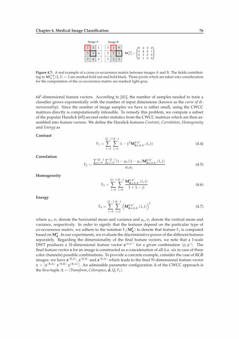
Chapter 4. Medical Image Classification 76
3
3 4
4
1
4
2
22
2 2
4
2
2
Image A
MA,B[0 1]
=
0 0 0 00 2 0 10 2 0 00 1 0 0
2 2
2 2
Image B
Figure 4.7: A real example of a cross co-occurrence matrix between images A and B. The fields contribut-ing to MA,B
[0 1](2, 2) = 2 are marked bold red and bold black. Those pixels which are taken into considerationfor the computation of the co-occurrence matrix are marked light-gray.
642-dimensional feature vectors. According to [41], the number of samples needed to train aclassifier grows exponentially with the number of input dimensions (known as the curse of di-
mensionality). Since the number of image samples we have is rather small, using the CWCCmatrices directly is computationally infeasible. To remedy this problem, we compute a subsetof the popular Haralick [65] second-order statistics from the CWCCmatrices which are then as-sembled into feature vectors. We define the Haralick features Contrast, Correlation, Homogeneityand Energy as
Contrast
F1 =
Q−1∑
i=0
Q−1∑
j=0
|i− j|2Mp,p′
d,s,k,k′(i, j) (4.4)
Correlation
F2 =
∑Q−1i=0
∑Q−1j=0 (i − µi)(j− µj)M
p,p′
d,s,k,k′(i, j)
σiσj
(4.5)
Homogeneity
F3 =
Q−1∑
i=0
Q−1∑
j=0
Mp,p′
d,s,k,k′(i, j)
1 + |i− j|(4.6)
Energy
F4 =
Q−1∑
i=0
Q−1∑
j=0
(
Mp,p′
d,s,k,k′(i, j))2
(4.7)
where µi,σi denote the horizontal mean and variance and µj,σj denote the vertical mean andvariance, respectively. In order to signify that the features depend on the particular type ofco-occurrence matrix, we adhere to the notation Fi(M
pd ) to denote that feature Fi is computed
based onMpd . In our experiments, we evaluate the discriminative power of the different features
separately. Regarding the dimensionality of the final feature vectors, we note that a J-scaleDWT produces a 3J-dimensional feature vector z(p,p′) for a given combination (p,p ′). Thefinal feature vector z for an image is constructed as a concatenation of all (i.e. six in case of threecolor channels) possible combinations. To provide a concrete example, consider the case of RGBimages: we have z(R,G), z(R,B) and z(B,G) which leads to the final 9J-dimensional feature vectorz = [z(R,G) z(R,B) z(B,G)]. An admissible parameter configuration ∆ of the CWCC approach isthe five-tuple ∆ = (Transform,Colorspace,d,Q, Fi).

Chapter 4. Medical Image Classification 77
4.2.3 Color “Eigen-Subbands”
The last feature extraction approach we discuss in the context of discriminant classifiers, isthe Color Eigen-subband (CES) approach we proposed in [99]. In order to overcome the shift-dependency problem of the DWT – caused by downsampling the filter outputs by two – wereplace the DWT by a non-subsampled variant known as the Stationary Wavelet Transform(SWT) [147]. This transform is implemented by the undecimated á-trous algorithm [165] andhas a redundancy factor of 3J, where J denotes the maximum decomposition depth. In the ter-minology of Palm [143], we aim for an integrative color-texture feature extraction approach. Byintegrativewe mean a technique which directly incorporates information among color channels.In contrast to that, it is always possible to artificially incorporate color channel informationby means of feature vector concatenation, see Section 4.2.1. However, the problem of featurevector concatenation is, that we neglect the association structure between the wavelet detailsubbands of different color channels. At least for the RGB colorspace, we have shown that theDWT/DTCWT transform coefficients exhibit a considerable degree of association, see Sections2.2.3 and 2.3.3. We strongly presume, that the situation is similar in case of the SWT.
To avoid the loss of information, we propose to compute statistics of PCA [41] decorrelateddetail subbands as image features. Decorrelation of color channels in the pixel domain is ex-ploited by Heeger & Bergen [67] in the context of texture synthesis. The reason why we performdecorrelation in the wavelet domain is rooted in the fact that decorrelation of the color channelsdoes not guarantee decorrelation of the transform coefficients, as Simoncelli et al. showed in[167]. However, Simoncelli et al. further point out, that decorrelation in the wavelet domainby means of PCA does not lead to decorrelated subband in all cases either. Instead of usingPCA, the authors propose to use Independent Component Analysis (ICA) as an alternative.Nevertheless, we retain the PCA approach, since the setup of [167] differs from our setup inthe following sense: in [167], the coefficient matrix is composed of transform coefficients fromall levels and all color channels by randomly selecting a collection of coefficients. In our setup,however, the coefficient matrix is constructed by selecting just the transform coefficients of thesame subband but on different color channels. Our experiments show that decorrelation of thetransform coefficients is acceptable in this special case, e.g. see Fig. 4.9. Further, computationof the PCA is less expensive than computation of ICA.
We next explain PCA-based decorrelation by means of an example: we assume RGB imagesand that each color channel is decomposed separately by a J-scale DWT. Without loss of gen-erality, we consider the k-th detail subband on decomposition level j, denoted by D
j,pk (the su-
perscript p denotes the color channel). The transform coefficients are denoted by cpi , 1 6 i 6 N
using linear indexing. We omit the subband and scale specifiers k and j for readability. Theconstruction of the coefficient matrix X is illustrated in Fig. 4.8. Each row of the matrix X isan observation vector ci ∈ R3. To decorrelate the components of the observation vector, PCAworks by diagonalizing the sample covariance matrix S, using the projection
S = ΦTSΦ (4.8)
where Φ denotes the matrix of eigenvectors corresponding to the eigenvalues of S (sorted inascending order). Since the sample covariance matrix S can be written as the product
S = ΦΛΦ with Λ =
λ1 0 00 λ2 00 0 λ3
(4.9)
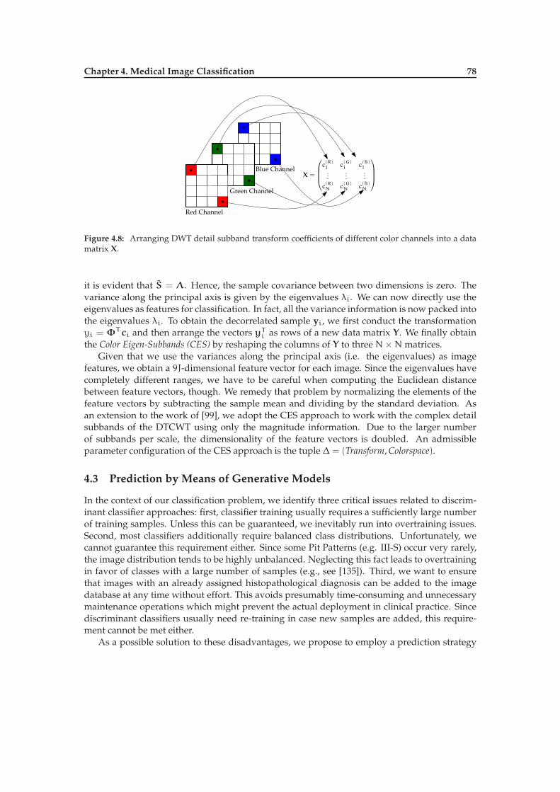
Chapter 4. Medical Image Classification 78
X =
c(R)
1c
(G)
1c
(B)
1
.
.
....
.
.
.
c(R)
Nc
(G)
Nc
(B)
N
Red Channel
Blue Channel
Green Channel
Figure 4.8: Arranging DWT detail subband transform coefficients of different color channels into a datamatrix X.
it is evident that S = Λ. Hence, the sample covariance between two dimensions is zero. Thevariance along the principal axis is given by the eigenvalues λi. We can now directly use theeigenvalues as features for classification. In fact, all the variance information is now packed intothe eigenvalues λi. To obtain the decorrelated sample yi, we first conduct the transformationyi = ΦT ci and then arrange the vectors yT
i as rows of a new data matrix Y . We finally obtainthe Color Eigen-Subbands (CES) by reshaping the columns of Y to threeN×Nmatrices.
Given that we use the variances along the principal axis (i.e. the eigenvalues) as imagefeatures, we obtain a 9J-dimensional feature vector for each image. Since the eigenvalues havecompletely different ranges, we have to be careful when computing the Euclidean distancebetween feature vectors, though. We remedy that problem by normalizing the elements of thefeature vectors by subtracting the sample mean and dividing by the standard deviation. Asan extension to the work of [99], we adopt the CES approach to work with the complex detailsubbands of the DTCWT using only the magnitude information. Due to the larger numberof subbands per scale, the dimensionality of the feature vectors is doubled. An admissibleparameter configuration of the CES approach is the tuple ∆ = (Transform,Colorspace).
4.3 Prediction by Means of Generative Models
In the context of our classification problem, we identify three critical issues related to discrim-inant classifier approaches: first, classifier training usually requires a sufficiently large numberof training samples. Unless this can be guaranteed, we inevitably run into overtraining issues.Second, most classifiers additionally require balanced class distributions. Unfortunately, wecannot guarantee this requirement either. Since some Pit Patterns (e.g. III-S) occur very rarely,the image distribution tends to be highly unbalanced. Neglecting this fact leads to overtrainingin favor of classes with a large number of samples (e.g., see [135]). Third, we want to ensurethat images with an already assigned histopathological diagnosis can be added to the imagedatabase at any time without effort. This avoids presumably time-consuming and unnecessarymaintenance operations which might prevent the actual deployment in clinical practice. Sincediscriminant classifiers usually need re-training in case new samples are added, this require-ment cannot be met either.
As a possible solution to these disadvantages, we propose to employ a prediction strategy

Chapter 4. Medical Image Classification 79
-200
0
200
-200
0
200
-200
-100
0
100
200
-400-200
0200
400
-50
0
50
-10
0
10
20
before PCA after PCA
GreenRed
Blu
e
Figure 4.9: Scatterplot of DWT subband transform coefficients (horizontal detail subband on DWT leveltwo of a Pit Pattern II image) before and after applying PCA. The pairwise (linear) correlation betweeneach component is approx. zero after PCA.
based on generative models. The baseline for this proposal is the framework of Bayesian imageretrieval [186] which we already discussed in Chapter 3. Considering the classification prob-lem from the viewpoint of image retrieval brings along several advantages which correspondto the requirements stated above. An unknown HMCC image is considered as a query imagein the probabilistic framework and classification is performed by first searching for the mostsimilar image in the database of available HMCC images with an assigned histological diagno-sis. Next, the class of the retrieved image is used as a prediction for the class of the unknownimage. In classification terminology, this resembles a nearest neighbor classifier. Fig. 4.10 showsthe two possible strategies for class prediction: (i) by searching for the feature representationpZ(z;Θr) which minimizes the KL divergence to the feature representation pZ(z;Θ∗) of theunknown image (left branch), or (ii) by searching the feature representation which maximizesthe (log) likelihood of the unknown image’s coefficient data (right branch). We don’t want togo into detail too much at this point, since the theoretical foundations are given in Chapter 3 towhich the reader is referred for further information. Eventually, we highlight the two strikingadvantages of the generative model based approach: first, no classifier training is required atall. Depending on which prediction strategy we use, it might not even be necessary to estimatethe model parameters of the query image (i.e. for likelihood maximization). Hence, we conse-quently avoid overtraining issues and are not tempted to overly optimize feature sets by meansof feature subset selection for example. Second, images with an existing histopathological diag-nosis can be added to the database at any time and are immediately available for future imagequeries.
4.4 Classification Setup
The classification setup for the discriminant classifier approaches is as follows: we restrict ourstudy to the one Nearest-Neighbor (1-NN) classifier we used in [98, 102, 64, 99, 100], since wefocus on a comparison of the various feature extraction approaches and do not conduct a studyon the performance of different classifiers. We further omit any feature subset selection or other

Chapter 4. Medical Image Classification 80
I∗
z∗
1, . . . , z∗
F
estimate Θ∗
d1 := D(pZ(z;Θ1)||pZ(z;Θ∗))...
dL := D(pZ(z;ΘL)||pZ(z;Θ∗))
d1 :=∑
K
i=1pZ(z∗
i;Θ1)
...
dL :=∑
K
i=1pZ(z∗
i;ΘL))
z∗
1, . . . , z∗
K
pZ(z;Θ∗)
r = arg mind1, . . . ,dL
⇒ assign label r to image I∗
r = arg maxd1, . . . ,dL
⇒ assign label r to image I∗
T T (e.g. DTCWT)
unknown Image
Figure 4.10: Prediction of the class label of an unknown image I∗ by means of (i) finding the featurerepresentation with the smallest KL divergence to the query image’s feature representation (left branch)or (ii) by searching for the feature representation which maximizes the log-likelihood of the query imagedata (right branch).
tuning steps to avoid overtraining issues. In case of the generative model based approaches, theclassification strategy is straightforward, since the class label of the retrieved image determinesthe class label of the unknown image anyway.
To obtain an estimate of classification accuracy, we use the method of Leave-One-Out Cross-validation (LOOCV) [41]. Given a dataset of L samples, LOOCV works by successively leavingout one sample of the whole dataset and performing the training procedure on the remainingL − 1 samples. The classification accuracy is then estimated as the number of times the left-outsample is correctly classified. Note, that in case of nearest neighbor classification paradigm, thetraining procedure just involves storage of the feature vectors. For the discriminant classifierapproaches, we rely on the Euclidean distance d(v,vj) = ‖vi − vq‖ between two feature vectorsvi and vj. As mentioned before, it is reasonable to conduct a normalization step before com-puting the Euclidean distance. This is accomplished by subtracting the mean and dividing bythe standard deviation. Formally, the normalized j-th element of feature vector vi is computedas vij = (vij − vj)/σ
2j . Of course, the standard deviation σj and the mean vj have to be repeat-
edly computed in each LOOCV iteration to ensure that no information of the left-out sample isincluded.
4.5 Experiments
We perform a comparison of the feature extraction approaches introduced in the context of dis-criminant classifiers and the approaches introduced in the context of generative models. In theformer case, we include the approaches of Gabor wavelets of Manjunath & Ma [117] (see Sec-tion 3.3.2), the WCS features of Van deWouwer et al. [35] and the color histograms proposed bySwain & Ballard [175] as a reference. Gabor wavelet features are commonly used in texture clas-sification and retrieval literature, WCS features have been successfully employed in the contextof endoscopic video frame processing [79] and the method of color histograms recently ap-

Chapter 4. Medical Image Classification 81
peared in context of computer-assisted Pit Pattern classification [63]. The latter two approachesare described below. In case of the generative model based approaches, we compare our re-trieval approaches of Sections 3.3 and Section 3.4 to the approaches of Vasconcelos & Lippman[186] and Verdoolaege et al. [188]. We refer the reader to Chapter 3 for a detailed descriptionof the retrieval approaches. Again, we adhere to the convention to identify an approach by thenames of the authors and the year of publication.
Van de Wouwer et al., 1997 In [35], Van de Wouwer et al. introduce the approach of Wavelet
Energy Correlation Signatures (WCS). The authors propose to decompose the color channelsof an image by a J-scale DWT and then calculate the correlation between all combinationsof subband pairs on different channels. In particular, given a RGB image and a three-scale DWT, we obtain 27-dimensional feature vectors. Since this approach can be easilyextended to work with the SWT and DTCWT, we will also consider these cases in ourexperiments. Note that in case of the DTCWT, the size of the feature vectors is doubled.
Swain & Ballard, 1991 The method of color histograms was introduced by Swain & Ballard[175] in an effort to evaluate whether color information can effectively capture imagecharacteristics. The authors compute three-dimensional histograms from the intensityvalues of each color channel. Since a full color histogram would consist of 2563 bins (verysparsely populated), intensity values are uniformly quantized to obtain a N1 × N2 × N3
bin color histogram withNi ≪ 256. This eventually allows computationally efficient sim-ilarity measurement using the histogram intersection as a similarity measure. For ourexperiments, we use the RGB color space and a quantization setting ofN1 = N2 = N3 = 8.
4.5.1 Image Acquisition
Our original set of images consists of 269 RGB images (53 patients, either 624× 533 or 586× 502pixel) acquired in 2005–2009 at the Department of Gastroenterology and Hepatology of theMedical University of Vienna using a zoom-endoscope (Olympus Evis Exera CF-Q160ZI/L)with amagnification factor of 150×. All imageswere selected by the gastroenterologist conduct-ing the colonoscopy with special emphasis to provide images with similar lightning conditionsat approximately the same camera angle. To enhance the visual appearance of the mucosa, dye-spraying with indigo-carmine was applied and biopsies or mucosal resections were taken toobtain a histopathological diagnosis (our ground truth). The histology was obtained by a pathol-ogist blinded to the colonoscopic procedure. Table 4.2 lists the histologies for the observed PitPatterns as well as the corresponding occurrences.
In order to increase the number of samples, we create an extended dataset by extracting256 × 256 pixel subwindows from the original images such that the Pit Patterns are clearlydistinctive and the subwindows contain a minimum number of specular reflections (see Fig.4.11). This resembles the clinical methodology during colonoscopy, since the gastroenterologistwill typically look at more than one region of an image. Finally, the extended dataset contains627 HMCC images distributed according to column #(extended) in Table 4.2.
In this thesis, we differ to the originally published works in one particular point. Up to now,the medical presentation of the problem was considered from a purely classification orientedpoint of view. In such a setup, it does not matter which image is selected as the one to predictthe class of an unknown image. The results, however, only convey an impression of how wellan approach captures image information relevant for discrimination. The classification rates areless meaningful from a medical point of view, though. This becomes obvious when we consider

Chapter 4. Medical Image Classification 82
Pit Pattern # #(extended) Histology #
I 36 114 Normal 36
II 26 64 Hyperplasia 26
III-S 12 18serrated Adenoma 4tubular Adenoma 8
III-L 44 119tubular Adenoma 43
tibulovillous Adenoma 1
IV120 232 tibulovillous Adenoma 115
Adenoma 2tubular Adenoma 3
V31 80 Lymphoma 6
Carcinoma 6Adenocarcinoma 19
∑269 627 269
Table 4.2: Pit Patterns with corresponding histopathological diagnosis. The second column, i.e. #, liststhe number of original images, while the third column, i.e. # (extended), lists the number of images in theextended dataset. The last two columns list the histologies and the corresponding occurrences.
specular reflection
Figure 4.11: Extraction of 256 × 256 pixel subwindows (black squares) from the original HMCC imageswith the objective to increase the dataset. Specular reflections in the first and third image are marked red.
our dataset extension technique and the fact that there is no restriction on the type of nearestneighbor simultaneously. In fact, during the LOOCV process, it is possible that the nearestneighbor stems from the same parent as the unknown image. In case we are only interested tofind images with similar visual content, this case does not pose a serious problem. Actually, theevaluation of texture retrieval systems works in the same way (see Section 3.3.2). Nevertheless,we can construct a clinically more relevant evaluation strategy by imposing a constraint onthe type of nearest neighbor. We say, that images are only admissible as nearest neighbors incase they do not stem from the same parent as the unknown image. We refer to this setup asthe constrained NN setup, whereas the setup in the original works will be referred to as theunconstrained NN setup. To visualize the difference, both types are illustrated in Fig. 4.12.

Chapter 4. Medical Image Classification 83
Parent 1 Parent 2 Parent 3
Constrained Nearest Neighbor
Unconstrained Nearest Neighbor
unknown Image
Figure 4.12: Illustration of the constrained and unconstrained nearest neighbor principle. In the un-constrained case, the nearest neighbor is allowed to stem from the same parent as the unknown image,whereas in the constrained case this is prohibited.
4.5.2 Parameter Configurations
In order to make our results reproducible, we have to define the parameter configurations forthe approaches. We first report the common parameters and then discuss the specific parametersettings. Regarding the choice of colorspace, we perform experiments using the RGB, HSV,YBR and YIQ colorspace. The conversions based on the RGB model are accomplished usingthe colorspace conversion routines of MATLAB. For all wavelet transform variants (includingGabor wavelets) the decomposition depth is fixed to J = 3 levels and no image preprocessingsteps are conducted. The Gabor wavelet settings (i.e. filter configurations) are listed in Section3.3.2.
Regarding the distribution feature approach of Section 4.2.1, color image processing is im-plemented by means of feature vector concatenation. In [64], our experiments showed thatfeature vector concatenation leads to competitive classification results compared to other, moreadvanced, combination strategies. Further, we use moment and ML estimates for the Gammaand Weibull parameters. This is a reasonable choice, since it allows to assess whether the es-timation methods have an impact on the classification results. This is similar to the retrievalscenario of Chapter 3, where we could show that the choice of parameter estimation methoddid not have any effect at all.
In case of the CWCC features of Section 4.2.2, we have several parameters which can be ad-justed. Regarding the quantization levels Q, we decided to conduct experiments using Q = 32and Q = 64 in order to keep the computational effort at a reasonable level. We strongly believethat this is a reasonable setting, since Karakanis et al. [79] reported no gain in classification ratesusing a higher number of quantization levels. The displacement vectors for the computation ofthe cross co-occurrence matrices are set to d = [0 0] (zero-displacement), d = [−1 1], d = [−1 0]and d = [−1 − 1]. We do not consider displacements that are farther away then one coefficient.In fact, we presume that a zero-displacement vector which corresponds to a multidimensionalcoefficient histogram will outperform any other displacement setting.
The WCS approach of Van de Wouwer et al. [35] and the Color-Eigen Subband (CES) ap-proach of Section 4.2.3 do not have any remaining free parameters.
4.5.3 Assessing Statistically Significant Differences
In any reasonable comparative study on classification performance, we face situations whereclassification rates between two approaches seem very similar and do not allow to make anystatements whether one approach performs better than the other. To evaluate whether the class

Chapter 4. Medical Image Classification 84
assignments of two approaches show statistically significant differences, we employ a McNe-mar test [46]. Besides the 5x2 cross-validation test, this is one of the most popular and recom-mended [37] tests for our purpose. The test statistic is based on counting the number of sampleswhere approach A assigns the right class label and approach B fails (denoted by n10) and viceversa (denoted by n01). Based on these counts, the test statistic is defined as
T =(|n10 − n01| − 1)2
n10 + n01. (4.10)
In case the null-hypothesis of no statistically significant difference is true, T follows as Chi-Square distribution with one degree of freedom, i.e. T ∼ χ21. Hence, given a fixed significancelevel α, we decide against the null-hypothesis if T > F−1
χ21(1 − α), i.e. when T is larger than the
(1−α) quantile of the Chi-Square distribution with one degree of freedom. For example, givenα = 0.05, we decide against the null-hypothesis if T > 3.84. Consequently, we can also say thatthere is enough evidence against the hypothesis of no significant differences.
Another important point in the context of evaluating differences between classifiers in ourcontext, is the issue of multiple comparisons. We perform multiple pairwise comparisons intwo variants. In order to assess whether a certain parameter configuration of an approach leadsto better LOOCV accuracy than other configurations, we select the best (i.e. the one with thehighest LOOCV accuracy) configuration and compare against the results obtained with all otherconfigurations. Hence, we consider a LOOCV run with one particular parameter configurationas a separate experiment. This is in accordance with the guidelines of Salzberg [157], wherethe author suggests that different parameter settings should be considered as a special caseof repetitive tuning. The second variant of the multiple comparisons scenario occurs when wecompare several distinct approaches to each other. In order to establish a reasonable ranking,we need to know if the results of two approaches are significantly different. As Salzberg [157]points out, such experimental settings require a correction of the significance level α of eachtest. To highlight the problem, lets consider the case wherewe performn pairwise comparisons.The chance of identifying a statistically significant result is 1− (1−α)n. It is straightforward tocheck that it only requires n = 45 comparisons in order to reach a probability > 90% of makinga false discovery (given independent experiments). The classic strategy to control the so calledFamilywise Error Rate (FWER) (i.e. the probability of making one or more Type I errors) is touse the Bonferroni correction, i.e. α is corrected to α = α/n, or a variant of the Bonferronimethod known as the Šidàk correction (see [157]). For our experiments, we implement thelatter method which corrects the significance level α to α = 1 − (1 − α)
1/n. For the example ofα = 0.05 and n = 45 we obtain α = 0.0011. Although this correction is based on the assumptionof independent tests – which might be violated in a practical scenario – it is still a reasonablestrategy to reduce the chance of making false conclusions. A second, alternative strategy to copewith the problem of multiple comparisons is to control the False Discovery Rate (FDR) instead ofthe FWER. The general difference to the aforementioned approach of using Bonferroni or Šidàkcorrection is, that the FDR focuses on the concept of discoveries, i.e. a statistically significantexperiment. The FDR is designed to control the rate of false discoveries which is a more naturalview of the problem in many situations. In this work, we implement the FDR control algorithmproposed by Benjamini & Hochberg [7]. Formally, given a set of n hypotheses with associatedp-values p1, . . . ,pn, we first sort the p-values to get p(1) 6 p(2) 6 · · · 6 p(n) and then determine
k = maxk : p(n) 6 α · k/n. (4.11)

Chapter 4. Medical Image Classification 85
Next, given that k exists, we reject the hypotheses corresponding to p(1), . . . ,p(k). Otherwise,no hypothesis is rejected at all. In the following, we refer to this procedure as the Benjamini-Hochberg procedure to control the FDR. Although, originally intended in situations where thehypotheses are independent, Benjamini & Yekutieli [8] show that in case the subset of teststatistics corresponding to true null-hypothesis are positively dependent, then the Benjamini-Hochberg procedure still controls the FDR at a level less than or equal to the desired level α.For our experiments, we make the assumption that the required condition can be met in case ofour test statistics. When providing significance results, we list the McNemar test outcome for(i) controlling the FWER by means of the Šidàk correction and (ii) controlling the FDR bymeansof the Benjamini-Hochberg procedure.
4.5.4 Results
As a starting point for our results section, we take a closer look at the three particular featureextraction approaches we discussed in the context of discriminant classifiers, see Section 4.2.We indent to identify the parameter configurations which lead to the top LOOCV rates andthen discuss whether we can claim superiority w.r.t. to the other configurations by means ofsearching for statistically significant differences.
First, we consider the CWCC features since this approach has the largest number of freeparameters. The LOOCV accuracies as well as the detailed classifier performance measuresof sensitivity/specificity as well as positive/negative predictive value (abbreviated by PPVand NPV, resp.) are listed in Table 4.3. We report, that the parameter configuration of ∆ =
(DTCWT,RGB,d = [0 0],Q = 32,Correlation) leads to the highest LOOCV accuracy of 89.63%in the two-class case. In case of the more fine grain discrimination of the three-class problem,the parameter configuration (SWT,YIQ,d = [0 0],Q = 32,Correlation) leads to the top rate of84.05%.
Problem Accuracy Sensitivity Specificity PPV NPV not sig.? (FWER/FDR)
2-class 89.63 84.83 91.54 79.89 93.84 22.11/11.63-class 84.05 - - - - 15.8/9.5
Table 4.3: Top LOOCV rates for the CWCC approach.
As we can see, specificity and the NPV are remarkably higher than the sensitivity and thePPV. This signifies that neoplastic disease can be diagnosed more reliably. Next, we fix the topparameter configurations and perform pairwise comparisons of the top results to the resultsobtained by the remaining parameter configurations. In Fig. 4.13a, we plot the sorted valuesof the McNemar test statistic T against the number of pairwise comparisons. The bold red-linesignifies the threshold (using FWER correction) above which we can claim statistically signifi-cant differences. Accordingly, Fig. 4.13d shows a plot of the sorted p-values against the numberof pairwise comparisons when relying on the Bejamini-Hochberg correction. The shaded areasignifies the region above which there is evidence against the null-hypothesis of the McNemartest. The percentage of non-significant differences among all pairwise comparisons is listedin the last column of Table 4.3. When tracing back the parameter configurations where thereis no evidence against the null-hypothesis, we observe the following situation: in almost anycase (no matter if we consider the two- or three-class problem) the Haralick feature Correlation

Chapter 4. Medical Image Classification 86
20 40 60 80
50
100
1502-class
3-class
Threshold: 11.9925
(a) CWCC (FWER corr.)2 4 6 8 10
5
10
15
20
25 2-class
3-class
Threshold: 8.1673
(b) CES (FWER corr.)5 10 15
0
5
10
15
20
2-class
3-class
Threshold: 9.0026
(c) Distribution Features (FWERcorr.)
20 40 60 80
0.2
0.4
0.6
0.8
2-class
3-class
(d) CWCC (FDR corr.)2 4 6 8 10
0.1
0.2
0.3
0.42-class
3-class
(e) CES (FDR corr.)5 10 15
0.2
0.4
0.6
0.8
1
2-class
3-class
(f) Distribution Features (FDRcorr.)
Figure 4.13: Illustration of the McNemar test outcomes for pairwise comparisons between the top param-eter configuration of each approach and the remaining parameter configurations. In the top row, we plotthe sorted McNemar test statistics T against the number of pairwise comparisons. The threshold (deter-mined using FWER control) above which we have evidence against the null-hypothesis is marked by abold red line. In the bottom row, we plot the sorted p-values against the number of comparisons. Theregion (determined using FDR control) of non-significant differences is marked gray.
and zero-displacement d = 0 are fix elements in the configuration. Only the colorspace andwavelet transform actually change. Practically, this allows to draw the conclusion that the Cor-relation feature together with a zero-displacement vector are the key elements to achieve goodclassification (and hence good prediction) results when using the CWCC approach.
We next turn to the results of the CES features. The free parameters of this approach are thetype of wavelet transform and the colorspace, hence there are twelve possible combinations.Table 4.4 lists the top LOOCV results for both classification problems. In either case, the high-est LOOCV accuracy, i.e. 93.14% and 88.84%, is obtained using the parameter configuration∆ = (DTCWT,YBR). When relying on control of the FWER, this configuration leads to signifi-cantly better classification results than any other configuration in≈ 19% and≈ 27% of all cases.The Benjamini-Hochberg procedure for FDR control is less strict, with ≈ 18% of non-significantresults for both problems. Again, identifying the pairwise comparisons where there is no ev-idence against the null-hypothesis, reveals that switching the colorspace from YBR to YIQ orRGB does not lead to a significant change in the classification results compared to the top pa-rameter configuration. Hence, the key parameter element of the CES approach is the choice ofwavelet transform, i.e. the DTCWT.

Chapter 4. Medical Image Classification 87
Problem Accuracy Sensitivity Specificity PPV NPV not sig.? (FWER/FDR)
2-class 93.14 86.10 96.14 90.45 94.21 18.8/18.23-class 88.84 - - - - 27.27/18.2
Table 4.4: Top LOOCV rates for the CES approach.
Finally, we take a look at the distribution features of Section 4.2.1. We include the mean &standard deviation of the subband coefficient magnitudes as features [102, 64] (denoted as En-ergy features). Since we can either use moment or ML estimation for the Gamma and Weibulldistribution parameters, we have 20 possible parameter configurations. For both classificationproblems, the configuration of ∆ = (YBR,Energy) leads to the highest LOOCV accuracies of93.30% and 89.47%, resp., see Table 4.5. Similar to Tables 4.3 and 4.4, the high rates for speci-ficity and NPV indicate better prediction performance of neoplastic disease. In the two-classcase, there is almost no significant difference in the results obtained by different parameter con-figurations. When we rely on FWER correction, this is also true for the three-class problem.However, in case of the FDR control approach, we report only ≈ 16% of non-significant differ-ences for the three-class problem. The detailed results reveal that the Energy features generallylead to higher discrimination rates, no matter which colorspace we choose. We attribute thiseffect to the bad choice of similarity measure (i.e. the Euclidean distance) for the distributionfeatures. As we will later see, the refinement of the similarity measure in favor of the KL diver-gence considerably improves the results.
Problem Accuracy Sensitivity Specificity PPV NPV not sig.? (FWER/FDR)
2-class 93.30 91.01 94.21 86.17 96.36 78.95/73.683-class 89.47 − − − − 57.89/15.8
Table 4.5: Top LOOCV rates for the distribution features approach.
After the fine-grain analysis of the feature extraction approaches, we go on to a comparativestudy of the CWCC, CES and distribution features (using the top parameter configurations) tothe Gaborwavelet features [117], color histograms [175] and theWCS features [35]. For the threereference approaches, we do not perform a detailed study whether there are statistically signif-icant differences in the results obtained by different parameter configurations. We simply pickout the best parameter configuration in each case. Tables 4.6 and 4.7 summarize the achievedLOOCV accuracies for the two- and three-class problem. In Table 4.7, we additionally list theclassifier performance measures of sensitivity, specificity, PPV and NPV for the discriminationof non-invasive vs. invasive disease. Accordingly, high values for specificity and NPV indicategood prediction performance for invasive neoplastic disease.
From Tables 4.6 and 4.7, we first notice that there is a considerable difference in LOOCVaccuracies between the top rates of 93.30%/89.47%and the worst rates of 84.34%/78.31%whichis equivalent to ≈ 60 more misclassified images. Further, specificity is higher than sensitivity inthe two-class case which suggests that the diagnostic accuracy of neoplastic disease is generallyhigher than for non-neoplastic disease (at least for our dataset). In case of the discrimination be-tween non-invasive and invasive neoplasia, the situation is reversed, see Table 4.7, with higher
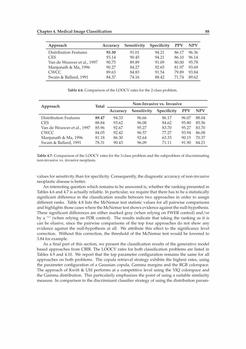
Chapter 4. Medical Image Classification 88
Approach Accuracy Sensitivity Specificity PPV NPV
Distribution Features 93.30 91.01 94.21 86.17 96.36CES 93.14 90.45 94.21 86.10 96.14Van de Wouwer et al., 1997 90.75 89.89 91.09 80.00 95.78Manjunath & Ma, 1996 90.27 84.27 92.65 81.97 93.69CWCC 89.63 84.83 91.54 79.89 93.84Swain & Ballard, 1991 84.37 74.16 88.42 71.74 89.62
Table 4.6: Comparison of the LOOCV rates for the 2-class problem.
Approach TotalNon-Invasive vs. Invasive
Accuracy Sensitivity Specificity PPV NPV
Distribution Features 89.47 94.33 96.66 86.17 96.07 88.04CES 88.84 93.62 96.08 84.62 95.80 85.56Van de Wouwer et al., 1997 85.96 92.67 95.27 83.70 95.27 83.70CWCC 84.05 92.42 96.57 77.27 93.94 86.08Manjunath & Ma, 1996 81.18 86.30 92.64 63.33 90.15 70.37Swain & Ballard, 1991 78.31 90.43 96.09 71.11 91.90 84.21
Table 4.7: Comparison of the LOOCV rates for the 3-class problem and the subproblem of discriminatingnon-invasive vs. invasive neoplasia.
values for sensitivity than for specificity. Consequently, the diagnostic accuracy of non-invasiveneoplastic disease is better.
An interesting question which remains to be answered is, whether the ranking presented inTables 4.6 and 4.7 is actually reliable. In particular, we require that there has to be a statisticallysignificant difference in the classification results between two approaches in order to assigndifferent ranks. Table 4.8 lists the McNemar test statistic values for all pairwise comparisonsand highlights those caseswhere theMcNemar test shows evidence against the null-hypothesis.These significant differences are either marked gray (when relying on FWER control) and/orby a ’∗’ (when relying on FDR control). The results indicate that taking the ranking as it iscan be elusive, since the pairwise comparisons of the top four approaches do not show anyevidence against the null-hypothesis at all. We attribute this effect to the significance levelcorrection. Without this correction, the threshold of the McNemar test would be lowered to3.84 for example.
As a final part of this section, we present the classification results of the generative modelbased approaches from CBIR. The LOOCV rates for both classification problems are listed inTables 4.9 and 4.10. We report that the top parameter configuration remains the same for allapproaches on both problems. The copula retrieval strategy exhibits the highest rates, usingthe parameter configuration of a Gaussian copula, Gamma margins and the RGB colorspace.The approach of Kwitt & Uhl performs at a competitive level using the YIQ colorspace andthe Gamma distribution. This particularly emphasizes the point of using a suitable similaritymeasure. In comparison to the discriminant classifier strategy of using the distribution param-

Chapter 4. Medical Image Classification 89
A B C D E F
A Distribution Features -B CES 0 -C Van de Wouwer et al, 1997. 4.50 2.92 -D Manjunath & Ma, 1996 4.10 3.70 0.05 -E CWCC 6.68∗ 5.63∗ 0.31 0.04 -F Swain & Ballard, 1991 26.07∗ 24.92∗ 11.35∗ 10.36∗ 8.64∗ -
A Distribution Features -B CES 0.23 -C Van de Wouwer et al, 1997. 6.30∗ 3.28 -D CWCC 8.38∗ 8.24∗ 1.06 -E Manjunath & Ma, 1996 19.41∗ 16.99∗ 6.37 2.18 -F Swain & Ballard, 1991 30.92∗ 28.54∗ 12.99∗ 7.65∗ 1.70 -
Table 4.8: McNemar test statistic values T for pairwise comparisons of the classification results for the2-class (top) and 3-class (bottom) problem in the context of the discriminant classifier based approaches.Test results, showing evidence against the null-hypothesis are marked shaded gray (when controlling theFWER) or by a ’∗’ (when controlling the FDR).
eters in conjunction with the Euclidean distance, the CBIR strategy relies on the well-foundedKL divergence and exhibits considerably better LOOCV rates. Regarding the approaches ofVasconcelos & Lippman [186] and Verdoolage et al. [188], we identify the YBR and RGB col-orspace as the most suitable configurations, respectively. A follow-up study on whether thereare significant differences in the classification results, however, reveals that there is no evidenceagainst the null-hypothesis for the majority of pairwise comparisons in the two-class case, seeTable 4.11. In fact, only the differences between the first and fourth approach in Table 4.9 and4.10 are significant. Based on the high classification rates we infer that only a few images aremisclassified. Consequently, the terms n10 and n01 in the computation of the McNemar teststatistic are rather small. This leads to low values of T which eventually explains the resultsof Table 4.11. In less technical terms, there is very little space for one approach to produce anotably different classification result compared to the other approaches. The final comparisonwe make is to compare the classification results achieved by the discriminant classifier basedapproaches to the top approach of the generative models, see Table 4.12. As we can see, allpairwise comparisons show evidence against the null-hypothesis of the McNemar test. Hence,it is safe to claim that the copula approach is at least superior to any of the approaches listed inTables 4.6 and 4.7.
Approach Accuracy Sensitivity Specificity PPV NPV
Copula 96.65 94.94 97.33 93.37 97.98Kwitt & Uhl, 2008 95.06 93.26 95.77 89.73 97.29Vasconcelos & Lippman, 2000 94.74 84.27 98.89 96.77 94.07Verdoolaege et al., 2008 92.98 91.01 93.76 85.26 96.34
Table 4.9: Comparison of the LOOCV rates for the 2-class problem.

Chapter 4. Medical Image Classification 90
Approach TotalNon-Invasive vs. Invasive
Accuracy Sensitivity Specificity PPV NPV
Copula 93.46 95.42 97.95 86.32 96.26 92.13Vasconcelos & Lippman, 2000 92.50 97.28 98.26 93.81 98.26 93.81Kwitt & Uhl, 2008 91.07 94.19 95.55 89.25 96.99 84.69Verdoolaege et al., 2008 88.52 93.35 96.36 82.42 95.21 86.21
Table 4.10: Comparison of the LOOCV rates for the 3-class problem and the subproblem of discriminatingnon-invasive vs. invasive neoplasia.
4.6 Discussion
Summarizing the results of this chapter, we make the following remarks: as with every discrim-inant classifier approach, the discriminative power of the feature set is the crucial factor for clas-sification performance. The most advanced classifiers can only find correct decision boundariesif the feature set captures the information that is essential to discriminate the classes. Further,discriminant classifiers usually depend on a user-supplied measure of similarity between twofeature vectors. Finding a reasonable similarity measure is not a trivial task in many situations,since feature vectors tend to be composed of many different kinds of features. Although thegeneric Euclidean distance works well in practice, it lacks a reasonable interpretation of the re-sulting value. Actually, we have seen that using the Euclidean distance for theWeibull/Gammadistribution features is suboptimal and performance can be considerably improved by a theo-retically well-founded dissimilarity measure such as the KL divergence. As a matter of fact, thevarious degrees of freedomwe have to cope with in a discriminant classifier scenario often leadto trial and error strategies in finding the most suitable configuration of feature set, similaritymeasure and classifier. In a generative model based approach, however, the degrees of free-dom are more restricted in a certain sense. Basically, only the choice of feature transformation
A B C D
A Copula -B Kwitt & Uhl, 2008 2.02 -C Vasconcelos & Lippman, 2000 2.88 0.01 -D Verdoolaege et al., 2008 11.25∗ 3.34 1.58 -
A Copula -B Vasconcelos & Lippman, 2000 0.39 -C Kwitt & Uhl, 2008 3.69 0.75 -D Verdoolaege et al., 2008 15.25∗ 6.06∗ 3.51 -
Table 4.11: McNemar test statistic values T for pairwise comparisons of the classification results for the2-class (top) and 3-class (bottom) problem in the context of the generative model based approaches. Testresults, showing evidence against the null-hypothesis are marked gray (when controlling the FWER) orby a ’∗’ (when controlling the FDR).

Chapter 4. Medical Image Classification 91
Approach 2-class 3-class
Copula − −
Distribution Features 9.30∗ 10.10∗
CES 8.48∗ 11.36∗
Van de Wouwer et al, 1997 24.45∗ 28.21∗
CWCC 26.41∗ 35.41∗
Manjunath & Ma, 1996 25.35∗ 49.36∗
Swain & Ballard, 1991 53.98∗ 63.56∗
Table 4.12: McNemar test statistic values for a pairwise comparison of the copula approach to all discrim-inant classifier approaches. Test results, showing evidence against the null-hypothesis are marked shadedgray (when controlling the FWER) or by a ’∗’ (when controlling the FDR).
and feature representation is up to the user. Once we have a suitable transformation and ananalytically tractable feature representation, we can at least follow the guidelines for selectingthe most similar image by relying on the Bayesian formulation of CBIR. Measuring similarityin terms of the maximum likelihood or the minimal KL divergence has a reasonable interpre-tation in this framework. Regarding a recommendation which strategy to choose in a clinicalapplication, it is hard to make a definitive statement. Although we tend to argue in favor of thegenerative model based strategy, we have also observed that significant differences in the clas-sification results are rare. It is possible that on another dataset, the margin between the copulaapproach and the discriminant classifier approaches shrinks and some significant differencesvanish. But this is a general issue of any classification problem when there is a lack of availabledata to perform a large scale study. Consequently, we argue that the conducted experimentsshould be considered as a prospective evaluation to select a collection of suitable approachesfor a final fusion stage, where various predictions of the histology are fused together to a finaldecision. This fusion might be based on weighting the different predictions by their reliabilityfor instance. However, this is topic of future research and beyond the scope of this thesis.

Chapter 5
Watermarking
In this chapter, we address the research topic of image watermarking, a branch of multimediasecurity where suitable statistical models of wavelet coefficients prove to be highly beneficial.Watermarking has been proposed as a technology to ensure copyright protection by embeddingan imperceptible, yet detectable signal in digital multimedia content such as images or video.According to Barni et al. [3], there is a strong resemblance between a watermarking system anda communication system. Embedding watermark information into some host (e.g. an image)asset resembles a transmission process. Any processing steps (e.g. compression, resizing) alongthe path of the watermarked asset to the receiver can be modeled as a communication channel.Eventually, recovery of the embeddedwatermark signal corresponds to the receiving side in thecommunication scenario. In order to identify and delineate the work of this chapter in the widefield of image watermarking, Fig. 5.1 shows a schematic overview of the watermarking systemconfiguration we rely on. As we can see, our focus is on the data recovery side and in particularon blind recovery of the watermark signal, i.e. when detection is performed without referenceto the unwatermarked host asset A. Further, our study is limited to the case of detectable wa-termarks (signified by the yes/no decision in Fig. 5.1) in contrast to readable watermarks. Inour configuration, the host interferes with the watermark signal. Hence, informed watermarkembedding and modeling the host signal are crucial for detection performance [116, 25]. Trans-form domains – such as the DCT or the DWT domain – facilitate modeling human perceptionand permit selection of significant signal components for watermark embedding. We followthe embedding strategy of additive embedding throughout this chapter, a technique which hasspawned many research articles in the last years. A plethora of different detectors has been pro-posed which all basically improve upon the particular statistical model for the host transformcoefficients [69, 139, 17, 125, 12].
The chapter is structured as follows: we start-off with a brief recapitulation of watermarkingas a statistical signal detection problem in Section 5.1. In Section 5.2, we introduce a novelwatermark detector based on the Cauchy distribution for DWT coefficients. Section 5.3 thenintroduces another novel detector, specifically tailored for color image watermarking. For bothdetectors, we conduct an extensive experimental study on the UCID image database [159] andcompare against a set of well-known watermarking approaches from literature. Regarding the
92

Chapter 5. Watermarking 93
w(K) Aw
Channel Data RecoveryA
′
w
A
yes/no
K
DWT IDWT
Topic of this Chapter
Embedding(DWT, spread-spectrum)
additive Embedding(e.g. HL subband)
A Aw
Embedding strength α
A . . . . . . . . . . . . . . . Host asset (i.e. image)K . . . . . . . . . . . . . . . . . . . . . . . .Key of PRNGw . . . . . . . . . . . . . . . . . (bipolar) WatermarkAw . . . . . . . . . . . watermarked Host Asset
Figure 5.1: Configuration of the watermarking system we use in this chapter (adapted form [3]).
contribution of this chapter, we highlight that major parts of the content recently appeared inthe following publications:
[94] R. Kwitt, P. Meerwald, and A. Uhl. A lightweight Rao-Cauchy detector for additive water-marking in the DWT-domain. In Proceedings of the ACM Multimedia and Security Workshop
(MMSEC ’08), pages 33–41, Oxford, UK, September 2008. ACM
[96] R. Kwitt, P. Meerwald, and A. Uhl. Color-image watermarking using multivariate power-exponential distribution. In Proceedings of the IEEE International Conference on Image Pro-
cessing (ICIP ’09), pages 4245–4248, Cairo, Egypt, November 2009. IEEE
5.1 Watermarking as a Signal Detection Problem
Regarding our description of the theoretical foundations, we closely adhere to the textbooks ofKay [83], Barni et al. [3] and Cox et al. [28]. The objective of this recapitulation is, to work outthe prerequisites to deploy different signal detection strategies for additive spread-spectrumwatermarking. We start from classic Neyman-Pearson detection and then successively loosenthe requirements on the specification of the host signal noise model. This leads to the idea ofGeneralized Likelihood Ratio testing (GLRT) and finally, to an asymptotically equivalent for-mulation of the GLRT known as the Rao hypothesis test. We follow the convention that thetransform coefficients of an arbitrary DWT detail subband are referred to as the host transformcoefficients x1, . . . , xN. The watermark signalw1, . . . ,wN is a realization ofN i.i.d. copies of a ran-dom variableW. For the purpose of additive spread-spectrum watermarking it is convenientto assume thatW follows a discrete uniform distribution with equiprobable values in +1,−1,hence, the corresponding p.m.f. ofW is given by
pW(x) =
0.5, if x = +1
0.5, if x = −1
0, else.
(5.1)

Chapter 5. Watermarking 94
The watermark signal is generated by a pseudo-random number generator (PRNG) seeded bysome secret key K. The rule for additive embedding can be formulated as
∀i : yi = xi + αwi (5.2)
where α > 0 denotes the embedding strength and the yi denote the watermarked transformcoefficients. The detection problem can be formulated as the detection of a deterministic sig-nal (i.e. the watermark) of unknown amplitude in incompletely specified noise. In terms ofhypothesis testing, we can state the null- (H0) and alternative hypothesis (H1) as
H0 : yi = xi (not/other watermarked), (5.3)
H1 : yi = xi + αwi (watermarked) (5.4)
which is equivalent to the (two-sided) parameter test
H0 : α = 0, (5.5)
H1 : α 6= 0. (5.6)
In the rare case that the p.d.f.s under both hypotheses can be completely specified, we can easilyconstruct a Neyman-Pearson (NP) detector which is optimal in the sense that it maximizes theprobability of detection Pd for a fixed probability of false-alarm Pf. Given that p(x;ΘH0) andp(x;ΘH1) denote the p.d.f.s under H0 and H1, then the Neyman-Pearson theorem states thatthe optimal detector decides in favor of H1 if
TL(x) =p(x;ΘH1)
p(x;ΘH0)> γ. (5.7)
The terms ΘH0 and ΘH1 denote the fully-specified parameter vector(s) of the noise model un-der H0 and H1, respectively. Eq. (5.7) is known as the Likelihood-Ratio Test (LRT) with thresholdγ [83]. In case we can deduce the distribution of the detection statistic TL(x) under H0, it isstraightforward to determine a suitable threshold for a fixed probability of false-alarm Pf as
γ = infx
(1 − F(x)) > Pf (5.8)
where F(x) denotes the distribution function of TL(x) under H0. For example, in case of a stan-dard Normal distribution, i.e. TL|H0 ∼ N(0, 1), the threshold can be expressed as
γ = Q−1(Pf) (5.9)
where Q−1 denotes the inverse Q-function to determine right-tail probabilities of the standardNormal distribution.
In order to constrain the probability of false-alarm, the NP test requires that the distribu-tion of the detection statistic under H0 does not depend on any unknown parameters. In caseswhere the noise model p.d.f.s under H0 and H1 cannot be fully specified, this requirement isusually violated. In fact, the embedding strength α as well as the distribution parameters of theassumed noise model might be unknown to the detector. Hence, in practice it is more realis-tic that we have to estimate the unknown parameters from the received signal. Nevertheless,a special case occurs when we assume that the host transform coefficients follow a Gaussiandistribution with parameters µ and σ. In that case, it is possible to design a NP test as if all

Chapter 5. Watermarking 95
parameters were known and obtain a LRT detection statistic which does not depend on the un-known parameters. This detector is commonly referred to as the linear-correlation (LC) detector[83]. In the general case though, it is not feasible to get rid of the unknown parameters.
When we cannot completely specify the noise distribution under both hypotheses, we haveto resort to composite hypothesis testing approaches. A common strategy to tackle the detectionproblem is to use a Generalized Likelihood Ratio Test (GLRT). This test replaces the unknown pa-rameters by the corresponding ML estimates conditioned on either H0 or H1. In the context ofwatermarking, this practically means that we have to estimate the embedding strength α fromthe received signal. For many noise models, however, estimation of α turns out to have no ex-plicit solution. In addition, the noise model parameters under H1 depend on α which furthercomplicates the estimation task. In the terminology of composite hypothesis testing, the noisemodel parameters are referred to as the nuisance parameters. Although, the focus is on testingα = 0 vs. α 6= 0, the parameters affect the detection statistics under both hypotheses as well.We follow the convention, that θs,H0 and θs,H1 denote the nuisance parameters under the null-and alternative hypothesis, respectively. The GLRT decides in favor of H1 if
TG(x) =p(x; α, θs,H1)
p(x; 0, θs,H0)> γ (5.10)
since α = 0 in case of H0. It is well-known, that the detection statistic 2 log TG(x) asymptotically(i.e. N→ ∞) follows
2 log TG(x)a∼
χ21, under H0
χ21(λ), under H1(5.11)
where χ21 denotes a Chi-Square distribution with one degree of freedom and χ21(λ) denotes anon-central Chi-Square distribution with one degree of freedom and non-centrality parameterλ, given by [82]
λ = α2[Iαα(0,θs) − Iαθs(0,θs)I
−1θsθs
(0,θs)Iθsα(0,θs)]. (5.12)
Two examples of the detection statistic p.d.f.s under H0 and H1 are shown in Fig. 5.2. By takinga closer look at Eq. (5.11), we see that the GLRT leads to a Constant False-Alarm Rate (CFAR)detector since the detection statistic distribution under H0 does not depend on any parametersat all. Hence, no matter which noise model we choose, the threshold needs to be calculatedjust one time. The terms Iαα, Iαθs
, Iθsα and Iθsθsin Eq. (5.12) denote partitions of the Fisher
information matrix, given by:
Iαα = E
[
∂ logp∂α
∂ logp∂α
]
1× 1 (5.13)
Iαθs= E
[
∂ logp∂α
∂ logp∂θs
]
1× s (5.14)
Iθsα = E
[
∂ logp∂θs
∂ logp∂α
]
s× 1 (5.15)
Iθsθs= E
[
∂ logp∂θs
∂ logp∂θs
]
s× s (5.16)
To show a practical example of how to derive a CFAR detector relying on the GLRT, weassume that the DWT detail subband coefficients can be modeled by a Gaussian distributionwith zero mean and variance σ2, i.e. X ∼ N(0,σ2). The example is similar to the one presented

Chapter 5. Watermarking 96
0 2 4 6 8 100
0.2
0.4
0.6
0.8
1
1.2
1.4
Detection Statistic Distribution under H0
TG
χ2 1
0 20 40 60 80 1000
0.01
0.02
0.03
0.04
0.05
T
χ2 1(λ
)
Pf = P(TG(x) > γ|H0)
Threshold γ = [Q−1(Pf/2)]2 = 1
λ = 24.59
Detection Statistic Distribution under H1
Figure 5.2: Illustration of the detection statistic distributions of the GLRT under H0 and H1 as well as theprobability of false-alarm Pf. The threshold is calculated for Pf ≈ 0.3.
in [82]. First, we need to determine the ML estimates of α and σ2 under both hypotheses. Toobtain the restricted MLE of α and σ2, i.e. the ML estimates under H1, we formulate the log-likelihood function as
L(α,σ;y1, . . . ,yN) = log(
1(2πσ2)N/2
)
−12σ2
N∑
i=1
(yi − αwi)2. (5.17)
Taking the derivative w.r.t. α and setting the resulting equation to zero gives
α =1N
N∑
i=1
yiwi (5.18)
as the MLE of α. The restricted MLE σ21 is obtained by taking the partial derivative of Eq. (5.17)w.r.t. σ and setting the corresponding term to zero. This gives
σ21 =1N
N∑
i=1
(yi − αwi)2 (5.19)
which, in combination with Eq. (5.18), finally allows to write the host signal noise p.d.f. underH1 as
p(x; α, σ21) =1
2πσ21exp
(
−N
2
)
. (5.20)
Under the null-hypothesis, we know that α = 0 and the MLE of σ2 – denoted as the unrestrictedMLE σ20 – is the sample variance of y1, . . . ,yN. Eventually, the detection statistic of the GLRTfor the CFAR detector is
2 log TG(x) = N logσ20σ21
. (5.21)
This detector is only asymptotically equivalent to the LC detector. However, we highlight thatthe threshold γ can be set to a predefined value and does not have be determined for each newsignal. Since the number of DWT coefficients N is usually quite large in case of images, we

Chapter 5. Watermarking 97
don’t have to worry about signal length issues related to the asymptotic performance of theGLRT. Letting Q−1
χ21denote the Q-function to express right-tail probabilities of the Chi-Square
distribution with one degree of freedom, γ can be set according to
γ = Q−1χ21(Pf) (5.22)
where Pf denotes the desired probability of false-alarm, e.g. Pf = 10−3. A presumably moreconvenient way to express γ is to rely on the relation that right-tail probabilities of the χ21 distri-bution can also be expressed by means of the Q-function to compute right-tail probabilities ofthe Gaussian distribution, i.e. Qχ2
1(x) = 2Q(
√x). Hence,
γ =
[
Q−1(
Pf
2
)]2
(5.23)
which is usually easier to handle due to existing implementations of the Gaussian Q-function.Fig. 5.2 illustrates a threshold (dashed line) of γ = 1 for Pf ≈ 0.32. In order to determine thenon-centrality parameter λ, we can rely on a theorem of Kay [82] which considers the specialcase of p(x;α,θs) = −p(x;α,θs). The theorem states that the symmetry of the noise modelleads to Iαθs
= 0 which reduces the expression in Eq. (5.12) to
λ = α2[Iαα(0,θs)]. (5.24)
In our example of a Gaussian host signal, we thus have λ = α2[Iαα(0,σ2)]. The correspondingpartition Iαα(α,σ2) of the Fisher information matrix can be derived from (see [82])
Iαα(α,σ2)] = E
[
(
∂ logp(xi − αwi;α,σ2
∂α
)2]
=
N∑
i=1
w2i
∫∞
−∞
[
p ′(n;α,σ2)p(n;α,σ2)
]2
p(n;α,σ2)dn
(5.25)wherewe have setni = xi−αwi and p ′(n;α,σ2) denotes the first partial derivative of p(n;α,σ2)w.r.t. n. After some calculus, we obtain
Iαα(0,σ2) =
N∑
i=1
w2i
1σ2
=N
σ2(5.26)
and the non-centrality parameter λ takes the form
λ = α2 N
σ2. (5.27)
An alternative approach to tackle the problem of composite hypothesis testing is to rely onthe asymptotic equivalence of the GLRT and the Rao hypothesis test [153]. The compellingadvantage of the Rao hypothesis test is that it does not require to compute ML estimates for αand θs under H1. Only the ML estimates under H0 are required for detection. Since we knowthat α = 0 in case of H0, the Rao test is particularly useful in situations where the embeddingside does not want to inform the detector about the choice of embedding strength. As pointedout by Barni et al. [3], this is an important degree of freedom, since it allows the embeddingside to adjust the embedding strength to the signal at hand. The Rao test decides H1 in case
TR(x) =∂ logp(x;Θ)
∂α
∣
∣
∣
∣
T
Θ=Θ
[
I−1(Θ)]
αα
∂ logp(x;Θ)
∂α
∣
∣
∣
∣
Θ=Θ
> γ (5.28)

Chapter 5. Watermarking 98
where Θ = [α θs,H0 ] denotes the ML estimates under H0, e.g. Θ = [0 σ20] for our previousproblem or Θ = [0 θs,H0 ] for a general nuisance parameter vector. Further, the term [I(Θ)]
−1αα is
given by
[I(Θ)]−1αα =
(
Iαα(Θ) − Iαθs(Θ)I−1
θsθs(Θ)Iθsα(Θ)
)−1(5.29)
where the partitions of the Fisher information matrix are defined in Eqs. (5.13) to (5.16). Due tothe asymptotic equivalence to the GLRT, the Rao hypothesis test inherits the distribution of thedetection statistic, i.e. TR(x) ∼ 2 log TG(x), see Eq. (5.11). Consequently, we obtain a CFAR detec-tor with the advantage to avoidML estimation of the embedding strengthα. In [139], Nikolaidiset al. first exploit this test to derive a watermark detector for additive spread-spectrum water-marks in the DWT domain, based on a Generalized Gaussian noise model. In Section 5.2, weintroduce a Rao hypothesis test conditioned on a Cauchy host signal noise model.
As a final remark of this section, we highlight that the Neyman-Pearson criterion is a quiteoverused term in watermarking literature. It is customary to derive a LRT-based detector forsome noise model and refer to the Neyman-Pearson criterion for threshold selection. This how-ever implies that we can actually constrain the probability of false-alarm which basically re-quires that the detection statistic under H0 does not depend on any unknown parameters. Tak-ing a closer look at popular detectors in literature, e.g. [69, 12], reveals that this is usually notthe case due to unknown noise parameters or unknown embedding strength. Given that weassume knowledge of the embedding strength at the detector, the noise parameters are stillunknown and have to be estimated from the received signal. Consequently, the resulting detec-tors are not NP detectors but rather estimate-and-plug detectors, as pointed out by Kay [83]. Thethreshold will be biased because the watermark may be present in the received signal. Never-theless, estimate-and-plug detectors are a reasonable choice in situations where the noise modelleads to intractable expressions for the GLRT or Rao hypothesis test.
5.1.1 Evaluation of Detector Performance & ROC curves
A critical issue with any watermarking system is how to evaluate the performance of the de-tector. A convenient strategy is to construct Receiver Operator Characteristic (ROC) curves.Although, we will later see that the ROC curve plots are disadvantageous when evaluating de-tection performance on a large number of images, the general construction principle is wortha discussion. Usually, we plot the probability of detection Pd (or miss Pm) in dependence ofthe probability of false-alarm Pf. In order to infer conclusions about the detector performancebased on ROC curves, we first have to ensure that the detector retains the desired Pf. This isan important point, since in any practical situation we expect the actual host signal noise todeviate from the theoretical model to some extent. In case of the GLRT or Rao test for instance,we have to check whether the detection responses under H0 in fact follow a Chi-Square distri-bution with one degree of freedom. Other detectors, e.g. the LC detector, require to verify thatthe detection statistic follows a Gaussian law. A reasonable way to perform these checks is toskip the embedding step and to call the watermark detectorM times on unwatermaked trans-form coefficients. This givesM detector responses, say ρ1, . . . , ρM, which we can use in a GoFtest to check if there is evidence against the null-hypothesis. In case there is no evidence, it issafe to set Pf to the desired level. Of course we could also count the number of false detectionsamong theM detector responses and compare against the expected number of false detections.However, this is computationally not feasible for small values of Pf (e.g. Pf = 10−10) which iswhy we favor the former strategy. The next step is, to determine Pm (or Pd). For that purpose,

Chapter 5. Watermarking 99
I
T
T−1
embed w
I ′′
J
detect w′
ρi
repeat M times
T
I ′
J ′
(a) other watermark (w 6= w ′)
I
T
T−1
embed wi
detect wi
ρ ′
i
repeat M times
T
I ′
I ′′
J J ′
(b) watermarked (wi = wi)
I
T
T−1
embed w
T
I ′
I ′′
J J ′
σ20, µ0
estimate
(c) estimate N(µ0, σ20)
Figure 5.3: Schematic process description of how to determine the detection responses under H0 (i.e.ρ1, . . . , ρM), H1 (i.e. ρ ′
1, . . . , ρ′M) and the calculation of the detection statistic parameters µ0 and σ20 from the
received signal.
we successively embed and detectMwatermarks to obtainM responses, say ρ′1, . . . , ρ′M ,under
H1. We can then estimate the corresponding detection statistic parameters under H1 and finallyplot the ROC curves. In case of a GLRT for instance, we can exploit the relationship [83]
Pd = Q(Q−1(1/2Pf) −√λ) +Q(Q−1(1/2Pf) +
√λ) (5.30)
to express Pd as a function of Pf and λ. The non-centrality parameter can be estimated byremembering that given X ∼ χ21(λ), it can be shown that
√X ∼ N(
√λ, 1) and thus
λ =
(
1N
N∑
i=1
√
ρ′i
)2
. (5.31)
Inserting λ in Eq. (5.30) gives the semi-experimentalROC curve. We use the term semi-experimentalsince a fully experimental ROC curve would imply counting of the number of missed detec-tions. The general expression to determine the semi-experimental probability of miss Pm is
Pm = P(T(x) < γ) = F(γ; b) (5.32)
where F denotes the c.d.f. of the detection statistic T under H1, parametrized by b. The semi-experimental evaluation strategy is of particular relevance when it comes to measuring theperformance of a detector under attacks. Due to the vast number of possible attacks on thewatermarked image, there is nowaywe could incorporate the attack characteristics into the hostsignal model in a tractable manner. As a matter of fact, evaluation of the watermark detectionperformance amounts to an experimental study. The semi-experimental way allows to plotROC curves even for low values of Pf. A graphical visualization of the whole strategy is shownin Figs. 5.3a and 5.3b where T denotes the transformation of an image I to a suitable transformdomain representation I ′, e.g. by a DWT. The watermarked image in the transform domain isdenoted by I ′′ and T−1 denotes the corresponding inverse transformation.
5.2 A Rao Hypothesis Test for Cauchy Host Signal Noise
One main motivation for deriving a novel watermark detector for host signal noise distributedother than Generalized Gaussian, is the fact that ML estimation of the GGD parameters is com-putationally expensive and requires a numerical root-finding procedure (see Chapter 3). Since

Chapter 5. Watermarking 100
the Cauchy distribution is a reasonable model for DWT transform coefficients and parameterestimation can be performed efficiently, chances are high that we can derive a computationallysimple and effective watermark detector. While other approaches such as [15] aim for a reduc-tion in watermark sequence length to enhance computational performance, we try to reduce thecomputational effort per step in the detection process. We start by deriving the first part of thedetection statistic of Eq. (5.28)
[
∂ logp(x;Θ)
∂α
]2
=
[
N∑
i=1
∂ logp(yi − αwi;γ)
∂α
]2
(5.33)
with Θ = [α γ]. Inserting the p.d.f. of the Cauchy distribution leads to
N∑
i=1
∂ logp(yi − αwi;γ)
∂α
(2.4)=
N∑
i=1
2wi(yi − αwi)
γ2(
1 +(yi−αwi)2
γ2
) . (5.34)
We next evaluate this expression at the ML estimate Θ = [0 γ] and take the power of two toobtain
[
∂ logp(x;Θ)
∂α
]2∣
∣
∣
∣
∣
Θ=Θ
= 4
[
N∑
i=1
yiwi
γ2 + y2i
]2
. (5.35)
In the second step, we need to derive an expression for
[I(Θ)]−1
= (Iαα(Θ))−1 (5.36)
which is the only term that is left over from Eq. (5.29), since we know that Iαθs= 0 in case of a
symmetric p.d.f. We modify Eq. (5.25) accordingly to obtain
Iαα(α,γ) =
N∑
i=1
w2i
∫∞
−∞
[
p ′(n;α,γ)
p(n;α,γ)
]2
p(n;α,γ)dn =1
2γ2
N∑
i=1
w2i =
N
2γ2. (5.37)
By using Eq. (5.28) and inserting the ML estimate Θ = [0 γ] under H0, we obtain the followingexpression for the detection statistic of our Rao hypothesis test conditioned on Cauchy hostsignal noise
TR(y) =
[
N∑
i=1
yiwi
γ2 + y2i
]28γ2
N. (5.38)
Based on Eq. (5.37) it is then straightforward to deduce the expression for the non-centralityparameter of the detection statistic under H1 as
λ = α2Iαα(0,γ) =Nα2
2γ2. (5.39)
We will next test our theoretical expressions by means of artificially generated data and thengo on to an experimental evaluation of the watermark detector on real data. Our test worksas follows: we generate Cauchy distributed host signal noise samples x1, . . . , xN as realizationsof N i.i.d. copies of a random variable X ∼ C(γ), where C(γ) denotes a Cauchy distributionwith shape parameter γ. We set γ = 5, N = 105 and generate the bipolar watermark sequence

Chapter 5. Watermarking 101
10-20
10-15
10-10
10-5
10-7
10-6
10-5
10-4
10-3
10-2
10-1
Probability of False Alarm
Pro
bab
ilit
yo
fM
iss
α = 0.2
α = 0.3
α = 0.4
α = 0.5
Figure 5.4: ROC curves for different embedding strengths of additively embedded (bipolar) watermarksin artificially generated Cauchy host signal noise samples with γ = 5,N = 10000.
wi as mentioned above. Further, we let the embedding strength α vary between 0.2 and 0.5with a stepsize of 0.1. From Eq. (5.39) we expect λ = 8, 18, 32, 50 for this setup. The detectorresponses under H0 and H1 are determined as illustrated in Figs. 5.3a and 5.3b withM = 1000.The ROC curves are shown in Fig. 5.4. Obviously, increasing the embedding strength leadsto better detector performance. The estimated values for the non-centrality parameter λ are8.68, 16.35, 32.47 and 50.94, resp., which conforms the validity of our derivation. For a practi-cal watermarking scenario, however, it is not a smart choice to set the watermarking strengtharbitrarily. In additive spread-spectrum watermarking, α is usually determined based on theData-to-Watermark (DWR) ratio, expressed in decibel (dB). In our context, the term Data refersto the DWT detail subband coefficients which we use for embedding. According to [3], theDWR is given by the expression
DWR = 10 log10
(
σ2xα2σ2w
)
(5.40)
where σ2x denotes the variance of the DWT detail subband coefficients and σ2w denotes thevariance of the watermarking sequence which in our case (i.e. bipolar watermark) equals 1.Hence, we can express the embedding strength α as a function of the DWR and the variance ofthe host signal as
α =
√
√
√
√
σ2x
exp(
log(10)·DWR10
) . (5.41)
The embedding strengths of the previous example (i.e. α = 0.2, 0.3, 0.4, 0.5)correspond to DWRsof 67.05dB, 61.53dB, 59.03dB and 57.09dB. As we can see, the DWR is rather high; reasonableDWRs for image watermarking are usually set to achieve a PSNR of 30dB to 50dB, i.e. the DWRis in the range of 12dB to 20dB.

Chapter 5. Watermarking 102
5.2.1 Experiments
To conduct a comparative study of detector performance, we have to introduce the experimentalsetup first. We use all images from the UCID image database. Since the original images are colorimages, we first conduct a conversion to grayscale images by means of MATLAB’s rgb2grayroutine. Then, we extract a 256× 256 pixel block from each image, starting in the top-left handcorner. Finally, all images are resized to 128 × 128 pixel using MATLAB’s imresize routinewhich basically performs bicubic interpolation.
We implement the following detectors for additive spread-spectrum watermarks: the nam-ing convention is, that the first part of the name denotes the host signal noise model and thesecond part denotes the type of hypothesis test. For example, Cauchy-LRT signifies that the hostsignal noise is modeled by a Cauchy distribution and the hypothesis test is a LRT. We highlightthat all mentioned LRT detectors are estimate-and-plug detectors and assume that the embed-ding strength α is known at the detection side.
Linear Correlator (Gaussian-LRT, LC) This detector arises when we derive a LRT for Gaussianhost signal noise, assuming that all parameters are known a-priori. It turns out, that theresulting detection statistic
T1(y) =1N
N∑
i=1
yiwi (5.42)
does neither depend on the noise distribution parameters nor on the embedding strengthand hence the resulting detector is a NP detector. The expressions for the mean and vari-ance of the detection statistic under H0 and H1 are given in [3].
Generalized Gaussian LRT (GGD-LRT) This detector is introduced by Hernandez et al. [69],based on the LRT and a Generalized Gaussian host signal noise model. The detectionstatistic is given by
T2(y) = ac
N∑
i=1
(
|yi|c − |yi − αwi|
c)
(5.43)
where the distribution parameters a and c are estimated from the received signal withoutcaring whether a watermark is present or not.
Cauchy LRT (Cauchy-LRT) This detector is introduced by Briassouli et al. [12] as an extensionof the GGD-LRT detector. The host signal noise is modeled by a Cauchy distribution andthe detection statistic is given as
T3(y) =
N∑
i=1
log(
γ2 + yi
γ2 + (yi − αwi)2
)
. (5.44)
Generalized Gaussian Rao (GGD-Rao) Nikolaidis et al. [139] first propose to use a Rao hy-pothesis test as a replacement of the plug-and-estimate detectors based on the LRT. Theirwork is motivated by the problem of informing the detector about the choice of α andthe bias introduced by estimating the noise distribution parameters from the received sig-nal. Based on the results of Kay [82], the authors derive a Rao test assuming GeneralizedGaussian host signal noise with the detection statistic given by
T4(y) =
(∑Ni=1 sgn(yi)wi |yi|
c−1)2
∑Ni=1 |yi|2c−2
(5.45)

Chapter 5. Watermarking 103
Detector µ0 6 µ0 σ20 6 σ20 ρ ∼ N(µ0, σ20) ρ ∼ N(µ0, σ20) ρ ∼ χ21 FP
GGD-LRT 98.36 15.40 88.57 2.54 - 0.1 · 10−3
Cauchy-LRT 98.43 41.03 96.83 2.39 - 0.1 · 10−3
Gaussian-LRT 62.63 59.34 97.16 95.07 - 0.9 · 10−3
Cauchy-Rao - - - - 82.88 1.7 · 10−3
GGD-Rao - - - - 99.48 0.8 · 10−3
Table 5.1: Evaluation whether the detection statistic distributions under H0 conform to the expected dis-tributions computed on the basis of the received signal. The numbers represent the percentage of UCIDimages where the test (given as column title) does not fail. The FP column lists the number of observedfalse positives.
where sgn(·) denotes the Signum function.
First, we verify that the detectors actually exhibit the theoretically stated detection statisticdistribution under the null-hypothesis, since this allows to set the detection threshold to a givenprobability of false-alarm. We verify that (i) the detector responses under H0 follow a Gaussiandistribution for all LRT detectors and a χ21 distribution for the Rao detectors; (ii) the detectionstatistic parameters µ0, σ20 calculated from the received signal (see Fig. 5.3c) correspond to thedetection statistic parameters µ0, σ20 estimated from the detection responses ρ1, . . . , ρM underH0. Due to the fact that we perform tests on all UCID images, we cannot directly compare thedetection statistic parameters by listing them in a table, such as in [69]. As an alternative, wechoose the following strategy: We perform a Chi-Square GoF test to check whether ρ1, . . .ρM ∼
N(µ0, σ20) or ρ1, . . . , ρM ∼ χ21, respectively. The results are listed in column five of Table 5.1.Except for the Gaussian-LRT detector, however, there is evidence against the null-hypothesis inmore than 90% of all cases. A closer look at the data reveals, that µ0 and µ0 differ considerablyin some cases. Nevertheless, the variances σ20 and σ
20 coincide to a large extent. Based on this
observation, we need to know whether the difference in mean has any negative effect on theprobability of false-alarm, i.e. whether the actually observed detection statistic distributionis shifted to the right. To rule out such a negative effect, we check if (i) µ0 6 µ0 and (ii) ifρ1, . . . , ρM ∼ N(µ0, σ20), see columns one and three of Table 5.1. Given that both tests show noevidence against the null-hypothesis, the detection threshold based on µ0 and σ20 is conservativein the sense that the probability of false-alarm will be lower than expected (see Fig. 5.5). Inthe last column of Table 5.1 we additionally list the number of observed false positives. Thenumbers are in quite good accordance to the predefined probability of false-alarm of Pf = 10−3.
Performance without attacks Due to the large amount of images, we cannot present classicROC curves to evaluate the performance of the detectors. Further, our objective is to as-sess the detector performance on the whole image database and not only on a selected setof images. In particular, we are more interested in the ranking of the detectors in criticalconditions, i.e. when Pm is high. This is reasonable, since in practice we are not concernedabout detector performance when Pm ≈ 10−100 for example. To provide such a compara-tive study, we fix the probability of false-alarm at a specified level, say 10−6, and constructa c.d.f. plot of the corresponding Pm values on a logarithmic scale for each detector. Wethen zoom-in on our Region of Interest (ROI), i.e. where Pm is high. To warrant this strat-egy, Fig. 5.7 shows the original c.d.f. plot on the left-hand side and a zoomed-in plot to

Chapter 5. Watermarking 104
-8 -6 -4 -2 0 2 4 6 80
0.05
0.1
0.15
0.2
0.25
0.3
0.35
µ0 = 1µ0 = −0.5
N(µ0, σ20)N(µ0, σ2
0)
shift to the left
Figure 5.5: Illustration of the difference in mean between the theoretically expected detection statisticdistribution N(µ0, σ20) and the empirically observed N(µ0, σ20). The red lines signify that the detectionthreshold is actually shifted to the left.
Figure 5.6: Four UCID images, ucid00246, ucid00444, ucid01059 and ucid01060 where allfive detectors fail to detect the watermark when embedding at a DWR of 12dB.
our ROI on the right-hand side. The DWR is set to 12dB for watermark embedding whichleads to an average PSNR of ≈ 42dB. Comparing both plots illustrates the point that theranking of the detectors changes as we move towards a higher probability of miss. In de-tail, we observe that although the GGD-LRT and Cauchy-LRT detectors exhibit far betterperformance then both Rao detectors when Pm < 10−100, the situation changes consider-ably when Pm > 10−4. We observe, that the LRT detectors perform poorly and even failin some cases while the Rao detectors still exhibit Pm values of < 10−2. The plots furtherhighlight, that presenting ROC plots for a small selection of images cannot provide fullinsight into the ranking of detectors. It is even possible, that the ROC curves for a fewimages might convey a completely wrong impression about detector performance. Wefurther note, that we can identify four UCID images where all detectors fail to detect thewatermark in our setup. These images were excluded from the plots and are shown inFig. 5.6. Detection failure occurs, since the embedding strength corresponding to a DWRof 12dB is too low for these images, resulting in no watermark presence.

Chapter 5. Watermarking 105
1e-300 1e-200 1e-100 10
0.2
0.4
0.6
0.8
1F(P
m)
Probability of Miss Pm
GGD-LRTCauchy-LRT
GGD-RaoCauchy-Rao
LC
1e-5 1e-4 1e-3 1e-2 1e-1 10.9
0.92
0.94
0.96
0.98
1
F(P
m)
Probability of Miss Pm
GGD-LRTCauchy-LRT
GGD-RaoCauchy-Rao
LC
Figure 5.7: C.d.f. plots of the probability of miss Pm for a fixed probability of false-alarm Pf = 10−6
and a DWR of 12dB over 1334 UCID images including a zoomed-in version of the region of interest,i.e. where Pm > 10−5.
Performance under attacks To evaluate the performance of the Cauchy-Rao detector under anattack, we choose JPEG compression with quality factors Q = 30 and Q = 70. The meanPSNR over the whole UCID image database for quality factorQ = 30 is ≈ 30dB, whereaswe obtain ≈ 33dB for quality factor Q = 70. In both cases, we fix the probability of false-alarm to Pf = 10−3, since for lower Pf values we do not get any reasonable results w.r.t ourlow image size of 128 × 128. As in the previous experiments, the watermark embeddingstrength is set to obtain a DWR of 12dB. Table 5.2 lists the test results when evaluatingthe detection statistic distribution under H0. We observe the interesting effect, that theactual detection statistic distributions are pretty close to the theoretical ones. ComparingTable 5.2 to Table 5.1 shows that there is no evidence against the null-hypothesis N(µ0, σ20)in almost all cases. Only for JPEG quality factor 30, the number of images where weobserve evidence against χ21 increases slightly. The c.d.f. plots of Pm over (almost) allUCID images are shown in Fig. 5.8. We again excluded the images shown in Fig. 5.6,since all detectors failed to detect the watermark. The left-hand side of Fig. 5.8 shows theunscaled versions of the c.d.f. plots and the right-hand side shows a zoomed-in version,where we focus on the most interesting region. In contrast to Fig. 5.7, the performance ofthe GGD-Rao detector strongly deteriorates and the LC detector starts to show acceptableperformance for quality factor Q = 30. A possible explanation for the poor results ofthe GGD-Rao detector is the negative impact of JPEG compression on the ML parameterestimation procedure of the GGD. Regarding the Cauchy-Rao detector, we observe stablebehavior over the whole range of Pm values. Even when Pm is high, the Cauchy-Raodetector exhibits acceptable performance.
5.2.2 Some Computational Considerations
As a final part of this section, we take a closer look at the computational requirements of eachdetector. This is a necessary step, since we originally proposed the Cauchy-Rao detector as alightweight alternative to the GGD-based detectors. In fact, low computational complexity wasa key motivation to derive a novel watermark detector. In particular, we consider the numberof arithmetic operations to calculate the detection statistics, briefly discuss parameter estima-

Chapter 5. Watermarking 106
Detector µ0 6 µ0 σ20 6 σ20 ρ ∼ N(µ0, σ20) ρ ∼ N(µ0, σ20) ρ ∼ χ21 FP
GGD-LRT [69] 66.44 54.11 97.53 95.94 - 0.96 · 10−3
Cauchy-LRT [12] 66.26 53.51 97.76 95.44 - 0.94 · 10−3
Gaussian-LRT 56.88 52.47 96.56 94.62 - 0.92 · 10−3
GGD-Rao [139] - - - - 72.50 0.66 · 10−3
Cauchy-Rao - - - - 74.96 0.45 · 10−3
GGD-LRT [69] 77.06 58.52 97.76 95.37 - 4.7 · 10−3
Cauchy-LRT [12] 78.33 59.04 97.98 95.81 - 1.5 · 10−3
Gaussian-LRT 59.49 51.12 97.46 96.79 - 0.9 · 10−3
GGD-Rao [139] - - - - 92.75 0.07 · 10−3
Cauchy-Rao - - - - 96.79 0.05 · 10−3
Table 5.2: Evaluation whether the detection statistic distributions under H0 conforms to the ex-pected distributions computed on the basis of the received signal under the influence of JPEG com-pression with quality factors Q = 30 (top) and Q = 70 (bottom). The numbers represent the per-centage of UCID images where the test (given as column title) does not fail. The column FP lists thenumber of observed false-positives.
tion issues and highlight the advantages of the Rao detectors w.r.t. threshold determination. Byarithmetic operations, we understand the number of additions & subtractions (+,−), multiplica-tions & divisions (×,÷), logarithms & exponentiations (log, pow) as well as computation of sgnand |·|. In Table 5.3, we provide the number of operations as a function of the input vector lengthN. From these numbers it is obvious, that the LC detector is by far the simplest one in terms ofarithmetic operations, since it involves only summations and multiplications of floating pointnumbers. Only the watermarked coefficients and the watermark sequence itself are involved.However, the Cauchy-Rao detector is only slightly more expensive, since the exponentiationsin Eq. (5.38) merely involve integer exponents. The remaining operations are just additions andmultiplications which can be very efficiently performed with few CPU cycles. In contrast tothat, the Cauchy-LRT detector requires N computations of the logarithm and the GGD-LRT aswell as the GGD-Rao detector even require exponentiations with floating point numbers, whichis very expensive in terms of CPU cycles.
Regarding parameter estimation issues, the LC detector is again the simplest one, since itrequires no parameter estimation at all, followed by the Cauchy-Rao and Cauchy-LRT detector,which both require to estimate the shape parameter γ of the Cauchy distribution, see Section2.2.2. In case of the detectors based on the GGD, we know that ML estimation of the shape cand scale parameter a requires to find the roots of a transcendental equation, see Section 2.2.1.Our estimation experiments confirm that the ML estimation of γ is faster by a factor of fourthan ML estimation of the GGD shape parameter c. When relying on the estimation proceduresuggested by Tsihrintzis et al. [176], see Eq. (2.6), estimation of γ is even linear in N.
Finally, we cover the effort for the determination of detection thresholds. In case of theLC, GGD-LRT and Cauchy-LRT detector, we have to compute the mean and variance of thenormally distributed detection statistic under H0 from the received signal yi to determine asuitable threshold. In contrast to that, the Cauchy-Rao and GGD-Rao detectors do not requireto compute detection statistic parameters at all, since they are CFAR detectors. A detectionthreshold needs to be computed only once from Eq. (5.23).

Chapter 5. Watermarking 107
1e-10 1e-5 10
0.2
0.4
0.6
0.8
1F(P
m)
Probability of Miss Pm
GGD-LRTCauchy-LRT
GGD-RaoCauchy-Rao
LC
1e-3 1e-2 1e-1 10.2
0.3
0.4
0.5
0.6
0.7
0.8
0.9
1
F(P
m)
Probability of Miss Pm
GGD-LRTCauchy-LRT
GGD-RaoCauchy-Rao
LC
(a) JPEG (Q = 30)
1e-100 1e-50 10
0.2
0.4
0.6
0.8
1
F(P
m)
Probability of Miss Pm
GGD-LRTCauchy-LRT
GGD-RaoCauchy-Rao
LC
1e-5 1e-4 1e-3 1e-2 1e-1 10.9
0.92
0.94
0.96
0.98
1
F(P
m)
Probability of Miss Pm
GGD-LRTCauchy-LRT
GGD-RaoCauchy-Rao
LC
(b) JPEG (Q = 70)
Figure 5.8: C.d.f. plots of the probability of miss Pm for a fixed probability of false-alarm Pf = 10−3
over 1334 UCID images under JPEG compression with quality factors Q = 30 and Q = 70. Theright-hand side shows a zoomed-in version of the region of interest, i.e. where Pm > 10−3 andPm > 10−5, respectively.
DetectorOperations
± ×,÷ | · |, sgn pow , logGaussian-LRT (LC), Eq. (5.42) N N + 1Cauchy-Rao, Eq. (5.38) 2N 3N+ 4GGD-LRT [69], Eq. (5.43) 3N N + 1 2N 2N+ 1Cauchy-LRT [12], Eq. (5.44) 3N 3N+ 2 N
GGD-Rao [139], Eq. (5.45) 2N+ 1 3N+ 2 2N N
Table 5.3: Number of arithmetic operations to compute the detection statistic.
5.3 Color Image Watermarking
Most of the watermarking research focuses on grayscale images. The extension to color imagewatermarking is usually accomplished by marking only the luminance channel or by process-ing each color channel separately [6]. However, it is well known that the human visual systemis least sensitive to the yellow-blue channel in the opponent representation of color, thus the

Chapter 5. Watermarking 108
HL Subband (Green)HL Subband (Red) HL Subband (Blue)
x1 = [x(R)
1 x(G)
1 x(B)
1 ]
xN = [x(R)
Nx
(G)
Nx
(B)
N]
Figure 5.9: Extraction of DWT coefficient vectors xi from three subbands (here HL) of different colorchannels.
watermark signal should be allocated to that band [158, 177]. In this section, we derive a novelwatermark detector for color image watermarking. We propose to use a multivariate statisticalmodel to capture the association structure between wavelet detail subbands across RGB colorchannels. Our objective is to show that watermark detection performance is improved, com-pared to decorrelating the color bands [4] or exploiting the correlation based on a Gaussian hostsignal model [6]. We highlight that we do not focus on perceptual shaping of the watermarksignal but on detecting the watermark in highly correlated color channels where the watermarkis embedded with constant strength.
5.3.1 A LRT detector for MPE host signal noise
We introduce an estimate-and-plug detector based on the LRT to detect an additively embeddedwatermark in host signal noise which follows a MPE distribution (see Section 2.2.3). For the fol-lowing derivation of the detector, we will rely on the convention that x denotes a 3-dimensionalvector of DWT coefficients, constructed by selecting one coefficient from the same detail sub-band of each color channel (illustrated in Fig. 5.9). We write x1, . . . , xN to refer to the coefficientvectors. Our watermarkwill be a realization ofN i.i.d. copies of a random variableW followinga discrete uniform distribution on +1,−1, see Eq. (5.1). The watermark sequence is denotedby w1, . . . ,wN. We follow the strategy to embed the same watermark in all three detail sub-bands. Given that 1 = [1 1 1] denotes a vector of ones, then the watermark vector to mark xi
can be written as wi = wi1. According to the rule of additive spread-spectrum watermarking,it follows that
∀i : yi = x + αwi (5.46)
where α > 0 denotes the embedding strength and yi denotes a watermarked DWT coefficientvector. We could choose a separate embedding strength for each signal dimension, but for thesake of readability we focus on the most simple case here. The embedding process is completedby computing the inverse DWT, followed by a quantization step to limit the pixel values to[0, 255]. Based on this watermarking setting, we can formulate the two hypothesis for our signal

Chapter 5. Watermarking 109
detection problem as
H0 : y = x (no/other watermark), (5.47)
H1 : y = x + αw (watermarked). (5.48)
Since we assume that α is known at the detection stage (i.e. the embedder has informed thedetector about its choice of α), we end up with the problem of detecting a known signal inincompletely specified noise. We proceed by constructing a NP detector as if all parameterswere known for both H0 and H1 and see how far we can get. Assuming independence of theobservations x1, . . . , xN allows to formulate a LRT which decides H1 in case
T(y1, . . . ,yN) =
∏Ni=1 p(yi − αwi)∏N
i=1 p(yi)> γ. (5.49)
After taking the logarithm and inserting the p.d.f. of the MPE distribution, see Eq. (2.9), weobtain the test statistic
T(y1, . . . ,yN) = −12
N∑
i=1
(
(yi − αwi)TΣ−1(yi − αwi)
)β+
12
N∑
i=1
(
yTi Σ−1yi
)β(5.50)
where we have used the fact that non signal-dependent terms are absorbed into the thresholdγ. As we can see, the detection statistic depends on the host signal noise parametersΣ and β. Incase of a GLRT approach, we would have to estimate both parameters under H0 and H1 whichis analytically intractable. The estimate-and-plug detector, however, simply estimates the pa-rameters from the received signal yi. If we consider all terms of the summation in Eq. (5.50)as independent, we can apply the central limit theorem and conclude that T follows a Nor-mal distribution under H0 and H1 with parameters (µ0,σ20) and (µ1,σ21), respectively. Anotherdifficulty arises, since we cannot compute the expected value of T w.r.t. yi in closed-form. Al-ternatively, it is possible to consider yi as fixed and average over the watermark signal wi. Thisstrategy is also followed by Hernandez et al. [69] to derive the detection statistic parameters ofthe GGD-LRT. The expected value µ0 under H0 (note that yi = xi) then takes the form
µ0 = −14
N∑
i=1
(
(xi − α)T Σ−1(xi − α))β
+(
(xi + α)TΣ−1(xi + α))β
+12
N∑
i=1
(
xTi Σ−1xi
)β. (5.51)
To derive the variance σ20 of T under H0, we exploit the following relation: given that X denotesa random variable and k = const., we know that V(
∑X) =
∑V(X) and that V(X + k) = V. It
follows that
V(T |H0) = V
(
−12
N∑
i=1
(
(xi − αwi)TΣ−1(xi − αwi)
)β
)
(5.52)
using yi = xi. We further know, that V(kX) = k2V(X) which leads to
V(T |H0) =14
N∑
i=1
V
(
(
(xi − αwi)T Σ−1(xi − αwi)
)β)
. (5.53)
To deduce the expression for V(T(y1, . . . ,yN)), we remember that wi is our variable term andthat the elements of wi follow a discrete uniform distribution on +1,−1. The variance of a

Chapter 5. Watermarking 110
random variableW with a discrete uniform distribution is given by
V(W) =12
2∑
i=1
w2i −
12
(
2∑
i=1
wi
)2
= 1 (5.54)
with w1 = −1 and w2 = +1. The variance of the detection statistic T under H0 then follows as
σ20 =116
N∑
i=1
(
(
(xi + α)TΣ−1(xi + α))β
−(
(xi − α)T Σ−1(xi − α))β)2
. (5.55)
Given that β, Σ denote the estimates of the MPE parameters – computed from the receivedsignal yi – we can insert these estimates into Eqs. (5.51) and (5.55) to obtain µ0 and σ20. Based ona chosen probability of false alarm Pf, it is then straightforward to set the detection threshold γas
γ = erfc−1(2Pf)
√
2σ20 + µ0. (5.56)
We consciously avoided the term Neyman-Pearson criterion to highlight that we cannot guar-antee to constrain the probability of false-alarm due to the reliance on the host signal noiseparameters (which are estimated). We can only say, that the threshold is selected in a Neyman-Pearson sense. We have to perform an empirical evaluation to ensure that we can constrainprobability of false-alarm. Regarding the detection statistic parameters (µ1,σ21) under the alter-native hypothesis H1, it can easily be shown that µ1 = −µ0 and σ21 = σ20.
5.3.2 Experiments
All following results are obtained on the whole UCID image database. Similar to the previousexperiments of Section 5.2.1, all images are cropped to 256 × 256 pixel, followed by a down-scaling stage to 128 × 128 pixel. The watermark is embedded in the HL subband on DWTdecomposition level two. Biorthogonal CDF 9/7 filters are used for DWT decomposition. Tocompare the performance of the proposed detector against two state-of-the-art detectors forcolor image watermarking, we implement the approaches proposed by Barni et al. in [4] and[6]. These approaches are briefly described next, including the parameter configuration we usein the experiments.
DCT-LRT In [4], Barni et al. propose to embed a watermark sequence into the mid-frequencyDCT coefficients obtained by computing a full-frame DCT on each color channel. In moredetail, the (k+1)-th to (k+n)-th DCT coefficients are selected in MPEG zigzag-scan orderfor watermark embedding, as shown in Fig. 5.10b. At the detection stage, the classic LCdetector is extended to the multichannel case. We point out, that the authors propose touse different embedding strengths for each channel, motivated by a study on how the Hu-man Visual System (HVS) perceives color stimuli at different wavelengths. The detectionstatistic is given by
T1(y1, . . . ,yN) =1N
N∑
i=1
wi(yR,i + yG,i + yB,i) (5.57)
where yR,i denotes the i-th watermarked DCT coefficient of the red color channel and wi
denotes the i-th element of the watermark sequence. The watermark is a realization of N

Chapter 5. Watermarking 111
i.i.d. copies of a random variableW ∼ N(0, 1). The authors show, that the detection statis-tic underH0 follows a zeromeanGaussian distributionwith variance given in [4]. This pa-rameter is estimated from the received signal. To choose the embedding strengths of eachchannel, we fix the total strength α and use the relations αR +αG +αB = α,αR/αG = 1.37as well as αB/αG = 3.24 to solve for αR,αG and αB.
FFT-LRT In [6], Barni et al. propose a different watermarking strategy based on decorrela-tion of the RGB color channels by means of the Karhunen-Loéve Transform (KLT). Thedecorrelated color channels are then transformed by the FFT. The basic idea is, that decor-relation allows to assume independency (at least in the Gaussian case) of the channels andleads to an analytically tractable joint statistical model for the magnitudes of the FFT co-efficients. However, we point out that some caution is advisable here, since decorrelatingthe color channels does not guarantee that the transform domain coefficients across colorbands are mutually decorrelated as well [107]. Basically, the approach is an extension ofthe work presented in [5] where the authors suggest a Weibull model for the magnitudesof FFT coefficients and derive a corresponding watermark detector based on the LRT. Thewatermark sequence is embedded in a diamond shaped region of the FFT domain (seeFig. 5.10a), defined by the (k + 1)-th to (k + n)-th diagonal of the first FFT quadrant.Separate embedding strengths per channel are proposed to take into account that the KLTleads to decorrelated channels with decreasing variance. Lets assume for a moment thatγ denotes the embedding strength and A,B,C denote the decorrelated color bands, thenthe detection statistic is given as
T2(y1, . . . ,yN) =∑
c∈A,B,C
N∑
i=1
yαc
c,i [(1 + γcwi)αc − 1]
[βc(1 + γcwi)]αc(5.58)
where αc,βc are the Weibull parameters estimated from the received FFT coefficient mag-nitudes of the c-th decorrelated color band.
For all following results, the embedding strength of each approach is chosen such that weobtain a mean PSNR of ≈ 50dB across the three RGB channels of an image. Further, we setk = n = 8000 in case of [4] and k = 30, n = 60 in case of [6]. This gives ≈ 8000 markedcoefficients for both the DCT and FFT approach (due to the symmetry of the FFT). For theproposed MPE-LRT detector, we choose the DWT HL subband on decomposition level two,resulting in ≈ 4000 marked coefficients in each channel.
Before we present the comparative study of the detection performance, we have to verifytwo important assumptions in order to ensure reasonable threshold selection. First, we verifythat the detector responses under both hypotheses follow a Gaussian law for all three detectorsby employing a Lilliefors test [108] at the 5% significance level. We report, that in no case thetest shows evidence against the null-hypothesis. Second, we have to ensure, that the detectionstatistic parameters µ0 and σ20 can be determined on the basis of the received signal. For thispurpose, we conduct a Monte-Carlo study withM = 1000 runs to obtain Table 5.41. The param-eters µ0 and σ20 again denote the detection statistic parameters estimated from the experimentalresponses under H0, i.e. ρ1, . . . , ρM (i.e. by sample mean and variance). Further, the column FP
lists the number of actually observed false positives. As we can see, the detection statistic pa-rameters of the MPE-LRT and DCT-LRT detector can be fairly well estimated from the received
1The remaining GoF tests are performed using a Chi-Square GoF test.

Chapter 5. Watermarking 112
k n
(a) FFT domain embedding [4]
(k+1)−th
(k + n)-th
(b) DCT domain embedding [6]
Figure 5.10: Watermark embedding location of the approaches [4] and [6]. In both works, the watermarkis embedded in mid-frequency coefficients of either the FFT [4] or DCT [6]. The symmetry of the FFTquadrants is indicated by marking coefficients with equal values in red and blue.
Detector µ0 6 µ0 σ20 6 σ20 ρ ∼ N(µ0, σ20) N(µ0, σ20) ρ ∼ N(µ0, σ20) FP
MPE-LRT 52.17 49.25 71.60 100.0 71.75 2.5 · 10−3
DCT-LRT [4] 52.09 48.61 99.93 100.0 99.93 1.0 · 10−3
FFT-LRT [6] 48.28 0.00 0.009 0.005 56.50 8.8 · 10−2
Table 5.4: Evaluation of the detection statistic distribution under H0 conforms to the expected distributioncomputed on the basis of the received signal. Then numbers represent the percentage of UCID imageswhere the test (given as column title) does not fail. The probability of false-alarm is set to Pf = 10−3.
signal. The percentage of observed false positives is in accordance with the fixed Pf value of10−3. In case of the FFT-LRT detector, however, the actually observed variance is larger thanexpected, resulting in a slightly higher number of false positives. In Fig. 5.11a, we show c.d.f.plots of the probability of miss over the whole UCID image database with a fixed Pf of 10−3.Compared to the DCT-LRT and FFT-LRT, the MPE-LRT shows superior performance, especiallyin the critical region where Pm is high. However, we note that there is a considerable numberof images where all detectors fail to detect the watermark. Due to the relatively low resolutionof the images (128 × 128) and the low embedding power to reach a mean PSNR of 50dB, thisresult is not unexpected, though. Fig. 5.11b shows the same plots, but choosing the DWR suchthat we achieve a mean PSNR of 40dB over the color channels of each image. We can see thatthe detectors of Barni et al. [4, 6] perform considerably better, but still the LRT-MPE shows thebest performance, even for high values of Pm.
5.4 Discussion
In this chapter, we introduced two novel detectors for additive spread-spectrumwatermarkingin the DWT domain. After a careful recapitulation of the prerequisites to deploy certain signal

Chapter 5. Watermarking 113
10−70 10−30 10−10 10
0.2
0.4
0.6
0.8
1F(P
m)
Barni et al., 2002 (DCT)Barni et al., 2002 (FFT)
MPE-LRT
Probability of Miss (Pm)10−50 10−2 1.5 · 10−1 0.1 0.5 1
0
0.2
0.4
0.6
0.8
1
Probability of Miss (Pm)
F(P
m)
Barni et al., 2002 (DCT)Barni et al., 2002 (FFT)
MPE-LRT
(a) Embedding strength set to achieve an average PSNR of 50dB
10−70
10−50
10−30
10−10
1
0
0.2
0.4
0.6
0.8
1
Probability of Miss (Pm)
F(P
m)
Barni et al., 2002 (DCT)Barni et al., 2002 (FFT)
MPE-LRT
10−20 10−15 10−10 10−5 10−1 10
0.2
0.4
0.6
0.8
1
Probability of Miss (Pm)
F(P
m)
Barni et al., 2002 (DCT)Barni et al., 2002 (FFT)
MPE-LRT
(b) Embedding strength set to achieve an average PSNR of 40dB
Figure 5.11: C.d.f. plots of the probability of miss Pm for a fixed probability of false-alarm Pf = 10−3 over1338 UCID images including a zoomed-in version on the ROI. The embedding strength was set to achievea mean PSNR (over the color channels) of 50dB (top) and 40dB (bottom).
detection strategies, we motivated the Rao hypothesis test as a lightweight alternative whichrequires very little knowledge about unknown parameters. We then derived a Rao hypothesistest conditioned on a Cauchy host signal noise model and showed that the detector exhibitsquite good performance compared to the state-of-the art detectors in this field. The Cauchy-Rao detector is also attractive from a computational point of view, since computation of thedetection statistic is comparable to the LC detector, estimation of the Cauchy shape parameteris less expensive than estimation of the GGD shape parameter and the computational demandfor threshold calculation vanishes at all.
In the second part of this chapter, we focused on the problem of color image watermarking.By relying on a multivariate model for DWT detail subband coefficients, we could derive anovel estimate-and-plug detector based on the LRT. A comparative study to two state-of-theart detectors revealed quite competitive performance of the novel detector on the whole UCIDimage database. The results of the MPE-LRT detector show that the association between theDWT coefficients can be efficiently exploited to enhance detection performance. Nevertheless,estimation of the MPE parameters is a computationally expensive operation which preventsdeployment of the MPE-LRT detector in computationally demanding scenarios.

Chapter 5. Watermarking 114
In the experimental sections of this chapter, we have further introduced a novel visual toolto evaluate detector performance. Motivated by the shortcomings of the classic ROC plots –which only allow to visualize detector performance on one image – we suggested a c.d.f. plotof the probability of miss at a fixed probability of false-alarm. We strongly believe that thisis a suitable way to study detector performance over a large set of images. To the best of ourknowledge, such a plot has not appeared in literature so far. Based on our experimental results,we come to a conclusion similar to Chapter 3. In general, it is not advisable to thoroughly relyon ROC curves to judge the quality of a detector. We rather suggest to fix the probability offalse-alarm, estimate the probability of miss and focus attention on the difficult cases.
Finally, we like to point out that a lot of questions remain unanswered and are topic of futureresearch. It seems promising to take a closer look at noise parameter estimation for example.In consideration of the variety of possible attacks, the question arises whether it is possible touse fixed parameter settings instead of ML estimation to stabilize detector performance. Thismight negatively affect performance in case of no attacks, but could be beneficial in situationswhere the attack distorts the coefficient statistics. Hernandez et al. [69] already suggesteda fixed setting of c = 0.8 for example. In addition to that, fixing the host noise parameterswould also contribute to the idea of lightweight detection and allow application of a detectorin scenarios where real-time performance is required, e.g. real-time detection of watermarksin video frames. Finally, the two novel detectors have to be evaluated under the influence ofcommon attacks. Since we strongly focused on the theoretical signal detection part, we omittedthe attack evaluation here and consider that as a topic for future work.

Chapter 6
Concluding Remarks
In this last part of the thesis, we recapitulate the main contributions and highlight future re-search directions. A general conclusion we draw from our studies is that there is still verymuch potential in developing novel statistical models for wavelet transform coefficients. Inthe context of this thesis, we could at least show that the models of Chapter 2 led to improve-ments upon state-of-the-art work in texture image retrieval, medical image classification andwatermarking research.
In particular, we showed that the proposed models for DTCWT coefficient magnitudes ledto a very lightweight probabilistic texture retrieval approach with remarkable retrieval per-formance. Incorporating coefficient dependencies across DTCWT subbands even further im-proved the retrieval results. However, the improvements in retrieval accuracy came at the costof degraded runtime which highlights the trade-off between model complexity and computa-tional performance. Surprisingly, the same statistical models turned out to be equally usefulfor medical image classification. We introduced a set of novel image features by refining exist-ing ideas from texture classification literature and demonstrated a high accuracy in predictinghistological diagnostic results from the visual appearance of colorectal lesions. Eventually, wepointed out the versatility of the statistical models by deriving two novel watermark detectorsfor luminance channel and color image watermarking. The detection experiments on a large setof images revealed competitive or even superior detection performance to current state-of-the-art detectors.
We summarize, that the particular field of application will eventually determine which sta-tistical model to use. In situations where computation time is a crucial factor for example, themost suitable model is useless in case the key processing steps become too complicated, eitheranalytically or computationally. In the context of watermarking for instance, a too complexmodel might substantially complicate the derivation of the detection statistic or even prevent todeduce a closed-form expression. In addition, parameter estimation issues might arise as well.A similar situation occurs in the context of probabilistic image retrieval, as we have pointed outby introducing two scenarios with different computational requirements. For a large number ofapplications, the following rule of thumb remains valid: the more information we incorporateinto a statistical model, the higher the price we pay in terms of runtime performance. There is
115

References 116
usually no such thing as a win-win situation in this context.
6.1 Future Research Directions
Finally, we remark that there are obviously many interesting topics we could not cover, or evenaddress, in this thesis and which remain part of future research. In consideration of the threefields of applicationwe discussed in this work, we like to highlight possible directions for futurestudies:
• In the context of texture image retrieval, we see great potential in a copula-based approachwhich incorporates the Generalized Gamma distribution [174] as a model for the margins.Since Choy & Tong [21] recently demonstrated better texture retrieval performance thanthe GGD based retrieval approach of Do & Vetterli [40], there is good reason to believethat a copula-based model would perform even better. Nevertheless, computational con-siderations will definitely play a key role for any practical application, since estimation ofthe Generalized Gamma model is computationally quite involved (e.g., see [172]).
• Concerning our particular watermarking setup of Chapter 5, the issue of how to combinedetection responses from different detection processes is a neglected topic in literature.The problem occurs, when we embed watermarks in more than just one DWT subbandand then try to combine the detection statistics into an overall detector response. Al-though a sum of i.i.d. Normal or Chi-Square random variables still follows a Normal orChi-Square distribution, application of the additivity property is only reasonable in caseof i.i.d. detection statistics. Since coefficients exhibit dependencies across subbands andthe detection statistic depends on the coefficients, this prerequisite is obviously violated.Consequently, this raises the question of how to constrain the probability of false-alarm.In fact, we presume that this problem calls for a flexible multivariate coefficient model,since this would remedy the fusion problem by shifting complexity to the modeling anddetector derivation stage.
• From our point of view, dealing with the fusion problem is a key issue for any furtherdevelopment of the computer-aided diagnosis system of Chapter 4 as well. Up to now,the majority of research work has focused on improving classification rates of standaloneapproaches. The only steps in the direction of combining prediction results were made in[62] or [61] with promising preliminary results. However, problems like overtraining is-sues or generalization quality still remain untreated. Finally, we suggest to further pursuethe generative model based prediction strategy because of the advantages with respect tothe aforementioned problems.
Although we have good reason to believe that other application areas, such as denoising orsegmentation will benefit from the proposed statistical models in a variety of ways, this remainsto be shown in future research work.

References
[1] M. Abramowitz and I.A. Stegun.Handbook ofMathematical Functions with Formulas, Graphs,and Mathematical Tables. Dover, New York, 1964.
[2] H. Akaike. A new look at the statistical model identification. IEEE Transactions on Auto-
matic Control, 19(6):716–723, December 1974.
[3] M. Barni and F. Bartolini. Watermarking Systems Engineering. Marcel Dekker, 2004.
[4] M. Barni, F. Bartolini, and A. Piva. Multichannel watermarking of color images. IEEE
Transactions on Circuits and Systems for Video Technology, 12(3):142–156,March 2002.
[5] M. Barni, F. Bartolini, A. De Rosa, and A. Piva. A new decoder for the optimum recoveryof non-additive watermarks. IEEE Transactions on Image Processing, 10(5):1–11, May 2001.
[6] M. Barni, F. Bartolini, A. De Rosa, and A. Piva. Color image watermarking in theKarhunen-Loeve transform domain. Journal of Electronic Imaging, 11(1):87–95, January2002.
[7] Y. Benjamini and Y. Hochberg. Controlling the false discovery rate: a practical and power-ful approach to multiple testing. Journal of the Royal Statistical Society – Series B, 57(1):289–300, 1995.
[8] Y. Benjamini and D. Yekutieli. The control of the false discovery rate in multiple testingunder dependency. The Annals of Statistics, 29(4):1165–1188, 2001.
[9] D. Berg. Copula Goodness-of-Fit testing: an overview and power comparison. The Euro-pean Journal of Finance, 15(7):675–701,October 2009.
[10] K. A. Birney and T. R. Fischer. On the modeling of DCT and subband image data forcompression. IEEE Transactions on Image Processing, 4(2):186–193, February 1995.
[11] E. Bouyé, V. Durrelman, A. Nikeghbali, G. Riboulet, and T. Roncalli. Copulas for finance– a reading guide and some applications. Working Paper, March 2000.
[12] A. Briassouli, P. Tsakalides, and A. Stouraitis. Hidden messages in heavy-tails: DCT-domain watermark detection using alpha-stable models. IEEE Transactions on Multimedia,7(4):700–715, August 2005.
117

References 118
[13] P. Brodatz. Textures: A Photographic Album for Artists and Designers. Dover Publications,New York, 1966. Pictures downloaded from http://www.ux.his.no/~tranden/brodatz.html(Trygve Randen).
[14] Robert W. Buccigrossi and Eero P. Simoncelli. Image compression via joint statistical char-acterization in the wavelet domain. IEEE Transactions on Image Processing, 8(12):1688–1701,December 1999.
[15] R. Chandramouli and N. D. Memon. On sequential watermark detection. IEEE Transac-
tions on Signal Processing, 51(4):1034–1044, April 2003.
[16] S. Chang, B. Yu, andMartin Vetterli. Spatially adaptivewavelet thresholding with contentmodeling for image denoising. In Proceedings of the IEEE International Conference on ImageProcessing (ICIP’98), Chicago, IL, USA, October 1998.
[17] Q. Cheng and T. S. Huang. An additive approach to transform-domain informationhiding and optimum detection structure. IEEE Transactions on Multimedia, 3(3):273–284,September 2001.
[18] H. Choi and R. Baraniuk. Multiscale texture segmentation using wavelet-domain hiddenmarkov models. In Proceedings of the Asilomar Conference on Signals, Systems, and Comput-
ers, pages 1692–1697, Pacific Grove, CA, United States, 1998.
[19] H. Choi, J.K. Romberg, R.G. Baraniuk, and N. G. Kingsbury. Hidden markov tree mod-eling of complex wavelet transforms. In Proceedings of the 2000 International Conference onAcoustics, Speech and Signal Processing (ICASSP 2000), Istanbul, Turkey, June 2000.
[20] S. C. Choi and R. Wette. Maximum likelihood estimation of the parameters of the Gammadistributon and their bias. Technometrics, 11(4):683–690, November 1968.
[21] S. K. Choy and C. S. Tong. Statistical wavelet subband characterization based on gener-alized gamma density and its application in texture retrieval. IEEE Transactions on ImageProcessing, 19(2):281–289, February 2010.
[22] R. J. Clarke. Transform Coding of Images. Academic Press, 1985.
[23] A. C. Cohen and B. J. Whitten. Parameter estimation in reliability and life space models.Marcel–Dekker, 1988.
[24] D. Comaniciu, P. Meer, P. Kun Xu, and D. Tyler. Retrieval performance improvementthrough low rank corrections. In Proceedings of the IEEE Workshop on Content-Based Accessof Image and Video Libraries (CBAIVL’99), pages 50–54, Fort Collins, CO, USA, 1999.
[25] M. Costa. Writing on dirty paper. IEEE Transactions on Information Theory, 29(3):439–441,May 1983.
[26] T. C. Cover and J. A. Thomas. Elements of Information Theory. Wiley, 1991.
[27] D. R. Cox and N. T. H. Small. Testing multivariate normality. Biometrika, 65(2), August1978.
[28] I. J. Cox, M. L. Miller, J. A. Bloom, J. Fridrich, and T. Kalker. Digital Watermarking and
Steganography. Morgan Kaufmann, 2007.

References 119
[29] M. S. Crouse, R. D. Nowak, and R. G. Baraniuk. Wavelet-based signal processing usingHidden Markov models. IEEE Transactions on Signal Processing, Special Issue on Waveletsand Filterbanks, 46(2):886–902, April 1998.
[30] K. J. Dana, B. V. Ginneken, S. K. Nayar, and J. J. Koenderink. Reflectance and texture ofreal world surfaces. In Proceedings of the IEEE International Conference on Computer Visionand Pattern Recognition (CVPR’97), pages 151–157, San Juan, Puerto Rico, 1997.
[31] MIT Vistion Texture Database. MIT vision and modeling group. [Online]. Available from:http://vismod.media.mit.edu/vismod/.
[32] I. Daubechies. Ten Lectures on Wavelets. Number 61 in CBMS-NSF Series in AppliedMath-ematics. SIAM Press, Philadelphia, PA, USA, 1992.
[33] J. G. Daugman. Uncertainty relation for resolution in space, spatial frequency, and orien-tation optimized by two-dimensional visual cortical filters. Journal of the Optical Society of
America, 2(7):1160–1169, July 1985.
[34] E. de Ves, A. Ruedin, D. Acevedo, C. Benavent, and L. Seijas. A new wavelet-basedtexture descriptor for image retrieval. Lecture Notes in Computer Science, Computer Analysisof Images and Patterns, 4673:895–902, August 2007.
[35] G. Van de Wouwer, S. Livens, P. Scheunders, and D. Van Dyck. Color Texture Classi-fication by Wavelet Energy Correlation Signatures. In Proceedings of the 9th InternationalConference on Image Analysis and Processing (ICIAP’97), pages 327–334, Florence, Italy, 1997.Springer.
[36] A. P. Dempster, N. M. Laird, and D. B. Rubin. Maximum likelihood from incomplete datavia the EM algorithm. Journal of the Royal Statistical Society – Series B, 39(1):1–38, 1977.
[37] T. G. Dietterich. Approximate statistical tests for comparing supervised classificationlearning algorithms. Neural Computation, 10(7):1895–1923,October 1998.
[38] M. Do. Fast approximation of Kullback-Leibler distance for dependence trees andHiddenMarkov models. IEEE Signal Processing Letters, 10(4):115–118, April 2003.
[39] M. Do and M. Vetterli. Rotation invariant texture characterization and retrieval us-ing steerable wavelet-domain hidden markov models. IEEE Transactions on Multimedia,4(4):517–527, December 2002.
[40] M. Do and M. Vetterli. Wavelet-based texture retrieval using Generalized Gaussian den-sity and Kullback-Leibler distance. IEEE Transactions on Image Processing, 11(2):146–158,February 2002.
[41] R. O. Duda, P. E. Hart, and D. G. Stork. Pattern Classification. Wiley & Sons, 2nd edition,November 2000.
[42] B. Efron and R. Tibshirani. An Introduction to the Bootstrap. Chapman & Hall/CRC, 1993.
[43] P. Embrechts, F. Lindskog, and A. McNeil. Modelling dependence with copulas and ap-plications to risk management. In S. Rachev, editor, Handbook of Heavy Tailed Distributionsin Finance, pages 329–384. Elsevier, 2003.

References 120
[44] A. N. Esgiar, R. N. G. Naguib, B. S. Sharif, M. K. Bennett, and A. Murray. Microscopic im-age analysis for quantitative measurement and feature identification of normal and can-cerous colon mucosa. IEEE Transactions on Information Technology in Biomedicine, 2(3):197–203, September 1998.
[45] M. Evans and N. Hastings B. Peacock. Statistical Distributions. Wiley Series in Probabilityand Statistics. Wiley, 3rd edition, 2000.
[46] B. Everitt. The Analysis of Contingency Tables. Chapman and Hall, 1977.
[47] B. Everitt. An R and S–Plus Companion to Multivariate Analysis. Springer, 2005.
[48] N. Fisher and P. Switzer. Graphical assessment of dependence: Is a picture worth 100tests? The American Statistican, 55(3):233–239, August 2001.
[49] J. H. Friedman and L. C. Rafsky. Multivariate generalizations of the wald-wolfowitz andsmirnov two-sample tests. Annals of Statistics, 7(4):697–717, 1979.
[50] K.-I. Fu, Y. Sano, S. Kato, T. Fuji, F. Nagashima, T. Yoshino, T. Okuno, S. Yoshida, andT. Fujimori. Chromoendoscopy using indigo carmine dye spraying with magnifying ob-servation is the most reliable method for differential diagnosis between non-neoplasticand neoplastic colorectal lesions: a prospective study. Endoscopy, 36(12):1089–1093, De-cember 2004.
[51] K. Fukunaga. Introduction to Statistical Pattern Recognition. Morgan Kaufmann, 2nd edi-tion, 1990.
[52] C. Genest and A. C. Favre. Everything you always wanted to know about Copula mod-eling and were afraid to ask. Journal of Hydrological Engineering, 12(4):347–368, July 2007.
[53] C. Genest and B. Rémillard. Validity of the parametric bootstrap for Goodness-of-Fittesting in semiparametric models. Annales de l’Institut Henri Poincaré, 44(6):1096–1127,2008.
[54] C. Genest, B. Rémillard, and D. Beaudoin. Goodness–of–fit tests for copulas: A reviewand a power study. Mathematics and Economics, 44:199–213, 2009.
[55] A. Genz. Numerical computation of multivariate normal probabilities. Journal of Compu-
tational and Graphical Statistics, 1(2):141–149, June 1992.
[56] A. Genz and F. Bretz. Comparison of methods for the computation of multivariate tprobabilities. Journal of Computational and Graphical Statistics, 11(4):950–971, December2002.
[57] J. Goldberger, S. Gordon, and H. Greenspan. An efficient image similarity measure basedon approximations of the KL-divergence between two Gaussian mixtures. In Proceedingsof the IEEE International Conference on Computer Vision (ICCV’03), pages 487–493, Nice,France, 2003.
[58] E. Gomez, M-A. Gomez-Viilegas, and J. M. Marin. A multivariate generalization of thepower exponential family of distributions. Communications in Statistics – Theory and Meth-ods, 27(3):589–600, 1998.

References 121
[59] R. M. Gray. Vector quantization. IEEE Transactions on Acoustic Signal and Speech Processing,1:4–29, April 1984.
[60] A. Gretton, K. Fukumizu, C.H. Teo, L. Song, B. Schölkopf, and A.J. Smola. A kernelstatistical test of independence. In Proceedings of the International Conference on Advances in
Neural Information Processing Systems (NIPS’07), pages 585–592, Vancouver, Canada, 2007.
[61] M. Häfner, A. Gangl, R. Kwitt, A. Uhl, A. Vecsei, and F. Wrba. Improving pit-patternclassification of endoscopy images by a combination of experts. In Proceedings of the In-ternational Conference on Medical Image Computing and Computer Assisted Intervention (MIC-
CAI’09), pages 247–254, London, UK, 2009.
[62] M. Häfner, A. Gangl, M. Liedlgruber, A. Uhl, A. Vécsei, and F. Wrba. Pit pattern classifi-cation using multichannel features and multiclassification. In D.I. Fotiadis T.P. Exarchos,A. Papadopoulos, editor,Handbook of Research on Advanced Techniques in Diagnostic Imaging
and Biomedical Applications, pages 335–350. IGI Global, Hershey, PA, USA, 2009.
[63] M. Häfner, C. Kendlbacher, W. Mann, W. Taferl, F. Wrba, A. Gangl, A. Vécsei, and A. Uhl.Pit pattern classification of zoom-endoscopic colon images using histogram techniques.In Johannes R. Sveinsson, editor, Proceedings of the 7th Nordic Signal Processing Symposium
(NORSIG 2006), pages 58–61, Reykavik, Iceland, June 2006. IEEE.
[64] M. Häfner, R. Kwitt, A. Uhl, A. Gangl, F. Wrba, and A. Vecsei. Feature-extraction frommulti-directional multi-resolution image transformations for the classification of zoom-endoscopy images. Pattern Analysis and Applications, 12(4):407–413,December 2009.
[65] R. M. Haralick, Dinstein, and K. Shanmugam. Textural features for image classification.IEEE Transactions on Systems, Man, and Cybernetics, 3:610–621, November 1973.
[66] N. A. Heckert and J. J. Filliben. NIST Handbook 148: DATAPLOT Reference Manual, vol-ume 1. National Institute of Standards and Technology Handbook Series, 2003.
[67] D. J. Heeger and J. R. Bergen. Pyramid-based texture analysis/synthesis. In Proceedings of
the International Conference on Computer Graphics and Interactive Techniques (SIGGRAPH’95),pages 229–238, Los Angeles, USA, 1995. ACM.
[68] N. Henze. A multivariate two-sample test based on the number of nearest neighbor typecoincidences. Annals of Statistics, 16(2):772–783, 1988.
[69] J. R. Hernández, M. Amado, and F. Pérez-González. DCT-domain watermarking tech-niques for still images: Detector performance analysis and a new structure. IEEE Transac-tions on Image Processing, 9(1):55–68, January 2000.
[70] G. W. Hill. Algorithm 396: Student’s t-quantiles. Communications of the ACM, 13(10):619–620, 1970.
[71] J. Huang and D. Mumford. Statistics of natural images and models. In Proceedings of the
IEEE International Conference on Computer Vision and Pattern Recognition (CVPR’99), pages1541–1547, Fort Collins, Colorado, United States, 1999.
[72] D. P. Hurlstone. High-resolution magnification chromoendoscopy: Common problemsencountered in “pit pattern” interpretation and correct classification of flat colorectal le-sions. American Journal of Gastroenterology, 97:1069–1070, 2002.

References 122
[73] D. P. Hurlstone, S. S. Cross, I. Adam, A. J. Shorthouse, S. Brown, D. S. Sanders, andA. J. Lobo. Efficacy of high magnification chromoscopic colonoscopy for the diagnosisof neoplasia in flat and depressed lesions of the colorectum: a prospective analysis. Gut,53(2):284–290, February 2004.
[74] D. K. Iakovidis, D. E. Maroulis, and S. A. Karkanis. An intelligent system for auto-matic detection of gastrointestinal adenomas in video endoscopy. Computers in Biologyand Medicine, 36(10):1084–1103,October 2006.
[75] D. K. Iakovidis, D. E. Maroulis, S. A. Karkanis, and A. Brokos. A comparative study oftexture features for the discrimination of gastric polyps in endoscopic video. In Proceed-
ings of the 18th IEEE Symposium on Computer-Based Medical Systems, 2005 (CBMS’05), pages575–580, Dublin, Ireland, June 2005.
[76] A. Jain and G. G. Healey. A multiscale representation including opponent color featuresfor texture recognition. IEEE Transactions on Image Processing, 7(1):124–128, January 1998.
[77] H. Joe. Multivariate Models and Dependence Concepts. Monographs on Statistics and Ap-plied Probability. Chapman & Hall, 1997.
[78] S. A. Karkanis, D. Iakovidis, D. Karras, and D. Maroulis. Detection of lesions in endo-scopic video using textural descriptors on wavelet domain supported by artificial neuralnetwork architectures. In Proceedings of the IEEE International Conference in Image Process-
ing, 2001 (ICIP’01), pages 833–836, Thessaloniki, Greece, October 2001.
[79] S.A. Karkanis. Computer-aided tumor detection in endoscopic video using color waveletfeatures. IEEE Transactions on Information Technology in Biomedicine, 7(3):141–152, Septem-ber 2003.
[80] S. Kato, K.-I. Fu, Y. Sano, T. Fujii, Y. Saito, T. Matsuda, I. Koba, S. Yoshida, and T. Fu-jimori. Magnifying colonoscopy as a non-biopsy technique for differential diagnosis ofnon-neoplastic and neoplastic lesions. World Journal of Gastroenterology: WJG, 12(9):1416–1420, March 2006.
[81] S. Kato, T. Fujii, I. Koba, Y. Sano, K. Fu, A. Parra-Blanco, H. Tajiri, S. Yoshida, and B. Rem-backen. Assessment of colorectal lesions usingmagnifiying colonoscopy andmucosal dyespraying: Can significant lesions be distinguished? Endoscopy, 33:306–310, April 2001.
[82] S. M. Kay. Asymptotically optimal detection in incompletely characterized non-gaussiannoise. IEEE Transactions on Acoustics, Speech and Signal Processing, 37(5):627–633,May 1989.
[83] S. M. Kay. Fundamentals of Statistical Signal Processing: Detection Theory, volume 2. Prentice-Hall, 1998.
[84] M. G. Kendall. A new measure of rank correlation. Biometrika, 30(1/2):81–93, June 1938.
[85] N. G. Kingsbury. The dual-tree complex wavelet transform: a new technique for shiftinvariance and directional filters. In Proceedings of the IEEE Digital Signal Processing Work-
shop, DSP ’98, pages 9–12, Bryce Canyon, USA, August 1998.
[86] N. G. Kingsbury. Image processing with complex wavelets. Phil. Trans. Royal SocietyLondon A, a DiscussionMeeting on “Wavelets: the key to intermittent information?”, September1999.

References 123
[87] N. G. Kingsbury. Complex wavelets for shift invariant analysis and filtering of signals.Applied and Computational Harmonic Analysis, 10(3):234–253,May 2001.
[88] Kazuo Konishi, Kazuhiro Kaneko, Toshinori Kurahashi, Taikan Yamamoto, MikiKushima, Akira Kanda, Hisao Tajiri, and Keiji Mitamura. A comparison of magnify-ing and nonmagnifying colonoscopy for diagnosis of colorectal polyps: a prospective.Gastrointestinal Endoscopy, 57:48–53, 2003.
[89] K. Krishnamoorthy. Handbook of Statistical Distributions with Applications. Chapman &Hall, 2006.
[90] S. M. Krishnan, X. Yang, K. L.Chan, S. Kumar, and P. M. Y. Goh. Intestinal abnormalitydetection from endoscopic images. In Proceedings of the 20thAnnual International Conferenceof the IEEE Engineering in Medicine and Biology Society, 1998 (EMBS’98), Hong Kong, China,October 1998.
[91] R. Krupinski and J. Purczynski. Approximated fast estimator for the shape parameter ofGeneralized Gaussian distribution. Signal Processing, 86(2):205–211, February 2006.
[92] S. Kudo, S. Hirota, T. Nakajima, S. Hosobe, H. Kusaka, T. Kobayashi, M. Himori, andA. Yagyuu. Colorectal tumours and pit pattern. Journal of Clinical Pathology, 47:880–885,1994.
[93] E. Kuruoglu and J. Zerubia. Modeling SAR images with a generalization of the Rayleighdistribution. IEEE Transactions on Image Processing, 13(4):527–, April 2004.
[94] R. Kwitt, P. Meerwald, andA. Uhl. A lightweight Rao-Cauchy detector for additivewater-marking in the DWT-domain. In Proceedings of the ACMMultimedia and Security Workshop
(MMSEC ’08), pages 33–41, Oxford, UK, September 2008. ACM.
[95] R. Kwitt, P. Meerwald, and A. Uhl. Blind DT-CWT domain additive spread-spectrumwatermark detection. In Proceedings of the 16th International Conference on Digital Signal
Processing, DSP ’09, Santorini, Greece, July 2009.
[96] R. Kwitt, P. Meerwald, and A. Uhl. Color-image watermarking using multivariate power-exponential distribution. In Proceedings of the IEEE International Conference on Image Pro-
cessing (ICIP ’09), pages 4245–4248, Cairo, Egypt, November 2009. IEEE.
[97] R. Kwitt, P. Meerwald, and A. Uhl. Efficient detection of additive watermarking in theDWT-domain. In Proceedings of the 17th European Signal Processing Conference, EUSIPCO’09, pages 2072–2076, Glasgow, UK, August 2009. EURASIP.
[98] R. Kwitt and A. Uhl. Modeling the marginal distributions of complex wavelet coeffi-cient magnitudes for the classification of zoom-endoscopy images. In Proceedings of the
IEEEComputer SocietyWorkshop onMathematicalMethods in Biomedical Image Analysis (MM-BIA’07), pages 1–8, Rio de Janeiro, Brasil, 2007.
[99] R. Kwitt and A. Uhl. Color eigen-subband features for endoscopy image classification. InProceedings of the 33rd IEEE International Conference on Acoustics, Speech and Signal Process-ing (ICASSP’08), pages 589–592, Las Vegas, Nevada, United States, 2008.

References 124
[100] R. Kwitt and A. Uhl. Color wavelet cross co-occurrence matrices for endoscopy imageclassification. In Proceedings of the 3rd International Symposium on Communications, Controland Signal Processing (ISCCSP’08), pages 715–718, St. Julians, Malta, 2008.
[101] R. Kwitt and A. Uhl. Image similarity measurement by Kullback-Leibler divergencesbetween complexwavelet subband statistics for texture retrieval. In Proceedings of the IEEE
International Conference on Image Processing (ICIP’08), pages 933–936, SanDiego, California,United States, October 2008.
[102] R. Kwitt and A. Uhl. Multi–Directional Multi-Resolution Transforms for Zoom–Endoscopy
Image Classification (Best Paper Award at CORES 2007), volume 45 of Advances in Soft Com-
puting, pages 35–43. Springer, 2008.
[103] R. Kwitt and A. Uhl. A joint model of complex wavelet coefficients for texture retrieval. InProceedings of the IEEE International Conference on Image Processing (ICIP ’09), pages 1877–1880, Cairo, Egypt, November 2009.
[104] R. Kwitt and A. Uhl. Lightweight probabilistic image retrieval. IEEE Transactions on Image
Processing, 19(1):241–253, January 2010.
[105] T. S. Lee. Image representation using 2D Gabor wavelets. IEEE Transactions on Pattern
Analysis and Machine Intelligence, 18(10):959–971,October 1996.
[106] J. Li, R. M. Gray, and R. A. Olshen. Multiresolution image classification by hierarchicalmodeling with two-dimensional HiddenMarkovmodels. IEEE Transactions on Information
Theory, pages 1826–1841, August 2000.
[107] Y. Liang, E. Simoncelli, and Z. Lei. Color channels decorrelation by ICA transformationin the wavelet domain for color texture analysis. In Proceedings of the IEEE Conference on
Computer Vision and Pattern Recognition, CVRP ’00, volume 1, pages 606–611. IEEE, June2000.
[108] H. Lilliefors. On the Kolmogorov-Smirnov test for normality with mean and varianceunknown. Journal of the American Statistical Association, 62:399–402, June 1967.
[109] J. Liu and P. Moulin. Information-theoretic analysis of interscale and intrascale de-pendencies between image wavelet coefficients. IEEE Transactions on Image Processing,10(11):1647–1658, November 2001.
[110] S. LoPresto, K. Ramchandran, and T. Orchard. Image coding based on mixture modelingof wavelet coefficients and a fast estimation–quantization framework. In Proceedings of the
Data Compression Conference (DCC’97), pages 221–230, Snowbird, Utah, USA, 1997.
[111] W.-Y. Ma and H.J. Zhang. Benchmarking of image features for content-based retrieval.In Proceedings of the Asilomar Conference on Signals, Systems & Computers, pages 253–257,Pacific Grove, California, United States, 1998.
[112] T. Mäenpää. The Local Binary Pattern Approach to Texture Analysis - Extensions and Applica-
tions. PhD thesis, University of Oulu, 2003.
[113] S. Mallat. A theory for multiresolution signal decomposition: The wavelet representation.IEEE Transactions on Pattern Analysis and Machine Intelligence, 11(7):674–693, July 1989.

References 125
[114] S. Mallat. A wavelet tour of signal processing. Academic Press, 1997.
[115] S. Mallat. A Wavelet Tour Of Signal Processing. Academic Press, 2nd edition, 1999.
[116] H. S. Malvar and D. A. F. Florencio. Improved spread spectrum: A new modulationtechnique for robust watermarking. IEEE Transactions on Signal Processing, 51(4):898–905,April 2003.
[117] B. S. Manjunath and W. Y. Ma. Texture features for browsing and retrieval of image data.IEEE Transactions on Pattern Analysis and Machine Intelligence, 18(8):837–842, August 1996.
[118] N. R. Mann and K. W. Fertig. Methods for Statistical Analysis of Reliability and Life Data.Wiley, 1974.
[119] J. Mao and A. K. Jain. Texture classification and segmentation using multiresolution si-multaneous autoregressive models. Pattern Recognition, 25(2):173–188, February 1992.
[120] K. V. Mardia. Measures of multivariate Kurtosis and Skewness. Biometrika, 57:519–530,1970.
[121] K. V. Mardia and P. Rupp. Directional Statistics, volume 2nd. John Wiley and Sons Ltd.,2000.
[122] D. E. Maroulis, D. K. Iakovidis, S. A. Karkanis, and D. A. Karras. CoLD: a versatile de-tection system for colorectal lesions in endoscopy video-frames. Computer Methods and
Programs in Biomedicine, 70(2):151–66, February 2003.
[123] J. R. Mathiassen, A. Skavhaug, and K. Bo. Texture similarity measure using Kullback-Leibler divergence betweenGamma distributions. In Proceedings of the European Conference
on Computer Vision (ECCV’02), pages 133–147, Copenhagen, Denmark, 2002.
[124] A. Meining, T. Rösch, R. Kiesslich, M. Muders, F. Sax, and W. Heldwein. Inter- and intra-observer variability of magnification chromoendoscopy for detecting specialized intesti-nal metaplasis at the gastroesophageal junction. Endoscopy, 36(2):160–164, February 2004.
[125] N. Merhav and E. Sabbag. Optimal watermark embedding and detection strategies un-der limited detection resources. IEEE Transactions on Information Theory, 54(1):255–274,January 2008.
[126] C. D. Meyer. Matrix Calculus and Applied Linear Algebra. Society for Applied and IndustrialMathematics, 2000.
[127] M. Mihcak, I. Kozintsev, and K. Ramchandran. Spatially adaptive statistical modelingof wavelet image coefficients and its application to denoising. In Proceedings of the 1999IEEE International Conference on Acoustics, Speech, and Signal Processing, ICASSP ’99, pages3253–3256, Phoenix, AZ, USA, March 2009. IEEE.
[128] M. A. Miller and N. G. Kingsburg. Statistical imagemodelling using interscale phase rela-tionships of complex wavelet coefficient. In Proceedings of the IEEE International Conference
on Accoustics, Speech and Signal Processing (ICASSP’06), pages 789–792, Toulouse, France,2006.

References 126
[129] M. A. Miller and N. G. Kingsburg. Image modeling using interscale phase propertiesof complex wavelet coefficients. IEEE Transactions on Image Processing, 17(9):1491 – 1499,September 2008.
[130] G. Moser, J. Zerubia, and S. Seprico. SAR amplitude probability density function es-timation based on Generalized Gaussian model. IEEE Transactions on Image Processing,15(6):1429–1442, June 2006.
[131] P. Switzer N. Fisher. Chi–plots for assessing dependence. Biometrika, 72:253–265, August1985.
[132] S. Nadarajah. The Kotz–type distribution with applications. Statistics, 37(4):341–358, July2003.
[133] S. Nadarajah. A generalized normal distribution. Journal of Applied Statistics, 32:685–694,September 2005.
[134] S. Nadarajah and S. Kotz. On the generation of gaussian noise. IEEE Transactions on Signal
Processing, 55(3):1172,March 2007.
[135] B. Mac Namee, P. Cunningham, S. Byrne, and O.I. Corrigan. The problem of bias intraining data in regression problems in medical decision support. Artificial Intelligence inMedicine, 24(1):51–70, January 2001.
[136] G. P. Nason and B. W. Silverman. The stationary wavelet transform and some statisticalapplications. Lecture Notes in Statistics, 103:281–300, 1995.
[137] R. B. Nelsen. An Introduction to Copulas. Springer Series in Statistics. Springer, secondedition, 2006.
[138] C. L. Nikias and M. Shao. Signal Prcocessing with Alpha–Stable Distributions and Applica-
tions. Wiley–Interscience, 1995.
[139] A. Nikolaidis and I. Pitas. Asymptotically optimal detection for additive watermarkingin the DCT and DWT domains. IEEE Transactions on Image Processing, 12(5):563–571,May2003.
[140] A. K. Nikoloulopoulos and D. Karlis. Copula model evaluation based on parametricbootstrap. Computational Statistics and Data Analysis, 52:3342–3353,March 2007.
[141] T. Ojala, M. Pietikäinen, and D. Harwood. A comparative study of texture measureswith classification based on feature distributions. Pattern Recognition, 29(1):51–59, January1996.
[142] T. Ojala, M. Pietikäinen, and T. Mäenpää. Multiresolution Gray-Scale and rotation invari-ant texture classification with local binary patterns. IEEE Transactions on Pattern Analysisand Machine Intelligence, 24(7):971–987, July 2002.
[143] C. Palm. Color texture classification by integrative co–occurrence matrices. Pattern Recog-
nition, 37(5):965–976,May 2004.

References 127
[144] C. Palm, T. M. Lehmann, and K. Spitzer. Color texture analysis of moving vocal cordsusing approaches from statistics and signal theory. In Proceedings of the 4th InternationalWorkshop on Advances in Quantitative Laryngoscopy, Voice and Speech Research, pages 49–56,2000.
[145] C. Palm, V. Metzler, B. Mohan O. Dieker, T. M. Lehmann, and K. Spitzer. Bildverar-beitung für die Medizin, chapter Co–Occurrence Matrizen zur Texturklassifikation in Vek-torbildern, pages 367–371. Springer, 1999.
[146] V. Panchenko. Goodness–of–fit tests for copulas. Physica A, 355(1):1–232, September 2005.
[147] J. C. Pesquet, H. Krim, and H. Carfantan. Time invariant orthonormal wavelet represen-tations. IEEE Transactions on Signal Processing, 44(8):1964–1970,August 1996.
[148] Maria Petrou and Pedro Garcia Sevilla. Image Processing. Texture: Dealing with Texture.Wiley John and Sons, 1st edition, 2006.
[149] R. Picard, T. Kabir, and F. Liu. Real-time recognition wih the entire Brodatz tex-ture database. In Proceedings of the IEEE International Conference on Pattern Recognition
(ICPR’93), pages 638–639, New York, United States, 1993.
[150] J. Portilla and E. Simoncelli. A parametric texture model based on joint statistics of com-plex wavelet coefficients. International Journal of Computer Vision, 40(1):49–70, October2000.
[151] S. M. Mahbubur Rahman, M. Omair Ahmad, and M. N. S. Swamy. Statistics of 2-d dt-cwtcoefficients for a gaussian distributed signal. IEEE Transactions on Circuits and Systems,55(7):2013–2025,August 2008.
[152] T. Randen and J.H. Husoy. Filtering for texture classification: A comparative study. IEEETransactions on Pattern Analysis and Machine Intelligence, 21(4):291–310,April 1999.
[153] C. R. Rao. Linear Statistical Inference and Its Applications. Probability and MathematicalStatistics. Wiley, 1973.
[154] J. Romberg, H. Choi, R. Baraniuk, and N. G. Kingsbury. Multiscale classification usingcomplex wavelets. In Proceedings of the IEEE International Conference on Image Processing(ICIP’00), volume 2, pages 371–374, Vancouver, Canada, 2000.
[155] J. K. Romberg, H. Choi, and R. G. Baraniuk. Bayesian wavelet domain image modelingusing hidden markov trees. In Proceedings of the IEEE International Conference on Image
Processing (ICIP’99), Kobe, Japan, October 1999.
[156] M. Rosenblatt. Remarks onmultivariate transformation. The Annals of Mathematical Statis-tics, 23(3):470–472, 1952.
[157] S. L. Salzberg. On comparing classifiers: Pitfalls to avoid and a recommended approach.Data Mining and Knowledge Discovery, 1(3):317–327, September 1997.
[158] E. Sayrol, J. Vidal, S. Cabanillas, and S. Santamaría. Optimum watermark detectionin color images. In Proceedings of the IEEE International Conference on Image Processing(ICIP’99), volume 2, pages 231–235, Kobe, Japan, October 1999.

References 128
[159] G. Schaefer and M. Stich. UCID - an uncompressed colour image database. In Proceedings
of SPIE, Storage and Retrieval Methods and Applications for Multimedia, volume 5307, pages472–480, San Jose, CA, USA, January 2004. SPIE.
[160] M. F. Schilling. Two-sample tests based on nearest neighbors. Journal of the American
Statistical Association, 81(395):799–806, September 1986.
[161] G. Schwarz. Estimating the dimension of a model. The Annals of Statistics, 6(2):461–464,March 1978.
[162] I. W. Selesnick, R. G. Baraniuk, and N. G. Kingsbury. The dual-tree complex wavelettransform - a coherent framework for multiscale signal and image processing. IEEE SignalProcessing Magazine, 22(6):123–151,November 2005.
[163] C. Shaffrey, N. G. Kingsbury, and I. Jermyn. Unsupervised image segmentation viamarkov trees and complex wavelets. In Proceedings of the IEEE International Conference on
Image Processing (ICIP’02), volume 3, pages 801–804, Rochester, New York, United States,2002.
[164] J.M. Shapiro. Embedded image coding using zerotrees of wavelet coefficients. IEEE Trans.
on Signal Process., 41(12):3445–3462,December 1993.
[165] M. J. Shensa. Wedding the à trous and Mallat algorithms. IEEE Transactions on Signal
Processing, 40(10):2464–2482, October 1992.
[166] J. K. Shuttleworth, A. G. Todman, R. N. G. Naguib, B. M. Newman, and M. K. Bennett.Colour texture analysis using Co–Occurrence matrices for classification of colon cancerimages. In Proceedings of the IEEE Canadian Conference on Electrical and Computer Engineer-
ing (CCECE’02), volume 2, pages 1134–1139,Winnipeg, Manitoba, Canada, 2002.
[167] E. Simoncelli and E. P. Zhibin Lei. Color channels decorrelation by ica transformation inthe wavelet domain for color texture analysis and synthesis. In Proceedings of the IEEEInternational Conference on Computer Vision and Pattern Recognition (CVPR’00), pages 606–611, South Carolina, USA, 2000.
[168] E.P. Simoncelli and W.T. Freeman. The Steerable Pyramid: A flexible architecture formulti-scale derivative computation. In Proceedings of the IEEE International Conference onImage Processing (ICIP’95), volume 3, pages 444–447,Washington, DC, USA, October 1995.
[169] M. Sklar. Fonctions de répartition àn dimensions et leursmarges. Publications de l’Institutede Statistique de l’Université de Paris, 8:229–231, 1959.
[170] S. P. Smith and A. K. Jain. A test to determine the multivariate normality of a data set.IEEE Transactions on Pattern Analysis and Machine Intelligence, 10(5), September 1988.
[171] K.-S. Song. A globally convergent and consistent method for estimating the shape pa-rameter of a Generalized Gaussian distribution. IEEE Transactions on Information Theory,52(2):510–527, February 2006.
[172] K.-S. Song. Globally convergent algorithms for estimating Generalized Gamma dis-tributions in fast signal and image processing. IEEE Transactions on Image Processing,17(8):1233–1250,August 2008.

References 129
[173] C. Spearman. The proof and measurement of association between two things. The Ameri-
can Journal of Psychology, 100(3/4):441–471, 1904.
[174] E. W. Stacy. A generalization of the gamma distribution. The Annals of Mathematical Statis-tics, 33(3):1187–1192, 1962.
[175] M.J. Swain and D.H. Ballard. Color indexing. International Journal of Computer Vision,7(1):11–32, November 1991.
[176] G.A. Tsihrintzis and C.L. Nikias. Fast estimation of the parameters of alpha–stable impul-sive interference. IEEE Transactions on Signal Processing, 44(6):1492–1503, June 1996.
[177] T. K. Tsui, X.-P. Zhang, andD. Androutsos. Color image watermarking using multidimen-sional fourier transforms. IEEE Transactions on Information Forensics and Security, 3(1):16–28, March 2008.
[178] S.-Y. Tung, C.-S. Wu, and M.-Y. Su. Magnifying colonoscopy in differentiting neoplasticfrom nonneoplastic colorectal lesions. American Journal of Gastroenterology, 96:2628–2632,2001.
[179] G. Tzagkarakis, B. Beferull-Lozano, and P. Tsakalides. Rotation-invariant texture retrievalwith Gaussianized Steerable Pyramids. IEEE Transactions on Image Processing, 15(9):2702–2718, September 2006.
[180] G. Tzagkarakis and P. Tsakalides. A statistical approach to texture image retrieval viaalpha-stable modeling of wavelet decompositions. In Proceedings of the 5th InternationalWorkshop on Image Analysis for Multimedia Interactive Services (WIAMIS ’04), Lisbon, Portu-gal, April 2004.
[181] P. Vandewalle, J. Kovacevic, and M. Vetterli. Reproducible research in signal processing -What, why, and how. IEEE Signal Processing Magazine, 26(3):37–47,March 2009.
[182] M. Varanasi and B. Aazhang. Parameteric Generalized Gaussian density estimation. Jour-nal of the Acoustical Society of America, 86(4):1404–1415,October 1989.
[183] N. Vasconcelos. On the efficient evaluation of probabilistic similarity functions for imageretrieval. IEEE Transactions on Information Theory, 50(7):1482–1496, July 2004.
[184] N. Vasconcelos and G. Carneiro. What is the role of independence for visual recogni-tion. In Proceedings of the European Conference in Computer Vision (ECCV’02), pages 297–311,Copenhagen, Denmark, 2002.
[185] N. Vasconcelos and A. Lippman. Library-based coding: A representation for effi-cient video compression and retrieval. In Proceedings of the Data Compression Conference(DCC’97), pages 121–130, Snowbird, Utah, USA, 1997.
[186] N. Vasconcelos and A. Lippman. A probabilistic architecture for content-based imageretrieval. In Proceedings of the IEEE International Conference on Computer Vision and Pat-
tern Recognition (CVPR’00), pages 1216–1221, Hilton Head, South Carolina, United States,2000.

References 130
[187] N. Vasconcelos and A. Lippman. A unifying view of image similarity. In Proceedings of
the International Conference on Pattern Recognition (ICPR’00), pages 38–41, Barcelona, Spain,2000.
[188] G. Verdoolaege and P. Scheunders S. De Backer. Multiscale colour texture retrieval usingthe geodesic distance between multivariate Generalized Gaussian models. In Proceed-ings of the IEEE International Conference on Image Processing (ICIP’08), pages 169 – 172, SanDiego, California, USA, 2008.
[189] A. Vo and S. Oraintara. A study of relative phase in complex wavelet domain: Property,statistics and applications in texture image retrieval and segmentation. Signal Procesing:Image Communication, 25(1):28–46, January 2010.
[190] M. J. Wainwright and E. P. Simoncelli. Scale mixtures of Gaussians and the statistics ofnatural images. In Advances in Neural Information Processing Systems (NIPS’99), volume 12,pages 855–861, Cambridge, MA, 2000. MIT Press.
[191] K. Xu, B. Georgescu, D. Comaniciu, and P. Meer. Performance analysis in content-basedretrieval with textures. In Proceedings of the International Conference on Pattern Recognition
(ICPR’00), pages 4275–4279,Washington, DC, USA, 2000.
[192] Q. Xu, J. Yang, and S. Ding. Color texture analysis using the wavelet-based hiddenmarkov model. Pattern Recognition Letters, 26(11):1710–1719,August 2005.
[193] K. Zografos. On Mardia’s and Song’s measures of Kurtosis in elliptical distributions.Journal of Multivariate Analysis, 99(5):858–879,May 2008.
Related Documents