1 Hyperspectral Band Selection from Statistical Wavelet Modelsmduarte/images/HBSSWM2016.pdf · 1 Hyperspectral Band Selection from Statistical Wavelet Models Siwei Feng, Student Member,

1

Hyperspectral Band Selection

from Statistical Wavelet ModelsSiwei Feng, Student Member, IEEE, Yuki Itoh, Student Member, IEEE,

Mario Parente, Senior Member, IEEE, and Marco F. Duarte, Senior Member, IEEE

Abstract

High spectral resolution brings hyperspectral images large amounts of information, which makes hyperspectral

images more useful in many applications than images obtained from traditional multispectral scanners with low

spectral resolution. However, the high data dimensionality of hyperspectral images increases the burden on data

computation, storage, and transmission; fortunately, the high redundancy in the spectral domain allows for significant

dimensionality reduction. Band selection provides a simple dimensionality reduction scheme by discarding bands

that are highly redundant, therefore preserving the structure of the dataset. This paper proposes a new criterion

for pointwise ranking-based band selection that uses a non-homogeneous hidden Markov chain (NHMC) model for

redundant wavelet coefficients of the hyperspectral signature. Wavelet-based modeling provides robustness to noise

thanks to the multiscale analysis performed by the transform. The model provides a binary-valued multiscale label

that encodes the presence of discriminating spectral information at different bands. A band ranking score considers

average correlation among the average NHMC labels for each band. We also test richer label vectors that provide

a more finely grained quantization of spectral fluctuations. In addition, since band selection methods based on band

ranking often ignore correlations in selected bands, we include an optional redundancy elimination step and test its

effect on band selection performance. Experimental results include a comparison with several relevant supervised

band selection techniques.

Index Terms

Band Selection, Hyperspectral Imaging, Wavelet, Hidden Markov Model

I. INTRODUCTION

Hyperspectral remote sensors collect reflected image data simultaneously in hundreds of narrow, adjacent spectral

bands, which make it possible to derive a continuous spectrum curve for each image cell. Compared with traditional

multispectral techniques generating image cubes with low spectral resolution, hyperspectral remote sensors obtain

a drastically increased number of spectral band. Such an increase in data dimensionality provides the potential

for better accuracy in discrimination among materials with similar spectral characteristics. However, one may

The authors are with the Department of Electrical and Computer Engineering, University of Massachusetts, Amherst, MA, 01003, USA.

E-mail: {siwei, yitoh}@engin.umass.edu, {mparente, mduarte}@ecs.umass.edu.

This work was supported by the National Science Foundation under grant number IIS-1319585.

2

ask whether all these hyperspectral bands are really necessary. In fact, such a large data volume is likely to

cause problems in data computation, storage, and transmission [1]. Moreover, hyperspectral images tend to include

significant redundancy in adjacent bands, leading to large amounts of redundant information [2]. All these drawbacks

of hyperspectral images present challenges to many conventional remote sensing data analysis problems. Thus,

dimensionality reduction is a necessary preprocessing step for hyperspectral data analysis.

One option for hyperspectral data dimensionality reduction is to transform the original data onto a low-dimensional

space while preserving a desired amount of information content. Such approaches are referred to as feature

extraction, in which the generated features are generally combinations of the original reflectance values. The

most popular feature extraction techniques include principal component analysis (PCA), which maximizes the

total variance of the selected features, and Fisher’s linear discriminant analysis (LDA), which maximizes the class

separability. A significant body of work exists on additional feature extraction techniques, such as orthogonal subset

projection (OSP) [3], projection pursuit (PP) [4], optimized information divergence projection pursuit (OIDPP) [5],

etc. However, the computation of new features requires the entire hyperspectral datacube to be acquired, which

increases the computational load to some extent. Morever, feature extraction changes the original data representation,

which complicates the interpretation of the results of relevant hyperspectral data analysis. Particularly, feature

extraction cannot be applied in cases where the physical meaning of individual bands needs to be maintained.

An alternative approach to dimensionality reduction is band selection [6–16], which is also referred to as feature

selection in the statistical literature. As a complement to feature extraction, band selection aims to select a subset

of the original bands, thus taking the advantage of preserving the same feature space as that of the raw data,

while avoiding the problem of high computational load as in feature extraction methods. For example, the Compact

Reconnaissance Imaging Spectrometer for Mars (CRISM) spectrometer has a tiling mode in which only 72 selected

channels are acquired [17]. The channels were carefully chosen to capture a sufficiently large set of spectral species

while maximizing the spatial filed of view.

Band selection methods can be roughly classified into two categories: groupwise selection methods [6–9] and

pointwise selection methods [10–16]. Groupwise selection methods aim at separating the entire set of spectral bands

into several subsets, and one representative is selected from each subset. All these selected bands or a part of them

form the final data representation. For example, [7] proposes a hierarchical clustering based method to separate

the spectrum into clusters by maximizing the ratio between intercluster variance and intracluster variance. For each

cluster, the band with the highest average correlation with other bands in the cluster is selected as the representative

band; the final band subset consists of representatives from each cluster. In [8], after the clustering procedure, clusters

whose representative bands are dissimilar to others will be eliminated. Representatives from remaining clusters form

the final output. In contrast, pointwise selection methods perform a gradual band selection procedure without relying

on partitioning. Pointwise selection methods can also be separated into two groups. Subset search methods [10–12]

aim at optimizing some criterion via search strategies, sequentially increasing or decreasing the number of selected

bands until the desired size is achieved. In contrast, band ranking methods [13–16] assign rankings to individual

bands to measure their priority in a given task based on some criteria; then, bands with higher rankings are selected.

3

Compared with subset search, band ranking does not need the computation of all possible combinations of band

subsets, therefore reducing the computational cost significantly. In terms of whether object class information is used

during band selection procedure, band selection approaches can be classified as either supervised or unsupervised.

Supervised band selection methods [9, 10, 12, 13, 15] assume a priori knowledge of the class label information for

different spectra during the selection process. In contrast, unsupervised band selection methods [6, 7, 11, 14, 18]

do not assume any prior class information. Finally, several semi-supervised band selection algorithms have recently

been proposed [8, 16], leveraging both labeled and unlabeled training samples for band selection.

In this paper, we propose a supervised pointwise hyperspectral band selection scheme featuring a non-homogeneous

hidden Markov chain (NHMC) model that is trained and applied on the wavelet transforms of the training and

testing spectra, respectively. The NHMC model provides significance labels (“large” and “small”) through Viterbi

algorithm for each wavelet coefficient based on the coefficient statistics among the training samples. The labels are

then collected into a binary feature matrix for each spectrum. The obtained binary features encode the scientifically

meaningful structural information of each pixel in a hyperspectral image, which are referred to as semantic features.

Instead of using the raw data, we use binary labels obtained by the NHMC model for each band and a variety of

scales for each pixel. We use these labels, averaged over each class, to calculate pair-wise class correlations for

each band as a criterion for ranking-based band selection.

Our previous work [19, 20] shows the advantages of the designed features in terms of hyperspectral classification,

which indicates the excellent discriminant performance of the designed features. Our main motivation of using those

features instead of raw data is their higher robustness to noise, which is likely to help reduce the negative influence

of noise on band selection, cf. Section II-C. To the best of our knowledge, neither wavelet analysis nor hidden

Markov models have been fully exploited in the field of hyperspectral band selection in the past.

We also present a comparison against some other supervised hyperspectral band selection methods, covering

both band ranking methods and subset search methods. The comparison involves several pixel-level classification

problems with hyperspectral images, and we use the classification accuracy as a performance metric for band

selection.

This paper is organized as follows. Section II reviews some related work and introduces the mathematical back-

ground behind our proposed band selection scheme. Section III provides an overview of the proposed hyperspectral

signature classification system. Section IV describes our experimental validation setup as well as the corresponding

results. Some conclusions are provided in Section V.

II. BACKGROUND AND RELATED WORK

In this section, we provide an overview of the NHMC models that will be used by our proposed method.

Furthermore, we review existing approaches to feature selection that will be used in the experimental section.

4

A. Wavelet Analysis

The wavelet transform of a signal provides a multiscale analysis of a signal’s content which effectively encodes

the locations and scales at which the signal structure is present in a compact fashion. In this paper, we use

the undecimated wavelet transform (UWT) to obtain multiscale analysis. We choose UWT because it provides

maximum flexibility on the choice of scales and offsets used in the multiscale analysis, which allows for a simple

characterization of the spectrum structure at each individual spectral band. Our analysis uses the Haar wavelet,

which is more sensitive to a larger range of fluctuations than other wavelets. Thus, the Haar wavelet enables the

detection of both slow-varying fluctuations and sudden changes in a signal [21], while it is not particularly sensitive

to small discontinuities (i.e., noise) on a signal, in effect averaging them out over the wavelet support.

A one-dimensional real-valued UWT of an N -sample signal x ∈ RN is composed of wavelet coefficients ws,n,

each labeled by a scale s ∈ 1, ..., L and offset n ∈ 1, ..., N , where L 6 N . The coefficients are defined using inner

products as ws,n = 〈x, φs,n〉, where φs,n ∈ RN denotes a sampled version of the mother wavelet function φ dilated

to scale l and translated to offset n:

φs,n(λ) =1√sφ

(λ− ns

).

All the coefficients can be organized into a two-dimensional matrix W of size L×N , where rows represent scales

and columns represent offsets. In this case, each coefficient ws,n, where s < L, has a child coefficient ws+1,n at

scale s+1. Similarly, each coefficient ws,n at scale s > 1 has one parent ws−1,n at scale s−1. Such a structure in the

wavelet coefficients enables the representation of fluctuations in a spectral signature by chains of large coefficients

appearing within the columns of the wavelet coefficient matrix W .

B. Statistical Modeling of Wavelet Coefficients

The statistical model is motivated by the compression property of wavelet coefficients, which states that the

wavelet transform of a piecewise smooth signal generally features a small number of large coefficients and a large

number of small coefficients. This property motivates the use of a zero-mean Gaussian mixture model (GMM) with

two Gaussian components to capture the compression property, where one Gaussian component (also called states)

with a high-variance characterizes the small number of “large” coefficients (labeled with a state L), while a second

Gaussian component with a low-variance characterizes the large number of “small” wavelet coefficients (labeled

with a state S). The state Ss ∈ {S,L} of a wavelet coefficient1 is said to be hidden because its value is not explicitly

observed. The likelihoods of the two Gaussian components pSs(L) = p(Ss = L) and pSs(S) = p(Ss = S) should

meet the condition that pSs(L) + pSs

(S) = 1. The conditional probability of a particular wavelet coefficient ws

given the value of the state Ss can be written as p(ws|Ss = i) = N (0, σ2i,s), where i = {S,L}, and the distribution

of the same wavelet coefficient can be written as p(ws) = pSs(L)N (0, σ2

L,s) + pSs(S)N (0, σ2

S,s).

1Since the same model is used for each chain of coefficients {S1,n, . . . , SL,n}, n = 1, . . . , N , we remove the index n from the subscript

for simplicity in this sequel whenever possible.

5

In cases where a UWT is used, the persistence property of wavelet coefficients [22, 23] (which implies the

high probability of a chain of wavelet coefficients to be consistently small or large across adjacent scales) can

be accurately modeled by a non-homogeneous hidden Markov chain (NHMC) that links the states of wavelet

coefficients in the same offset. Because of the overlap between wavelet functions at a fixed scale and neighboring

offsets, adjacent coefficients may have correlations in relative magnitudes [24]. However, for computational reasons,

in this paper we only consider the parent-child relationship of the wavelet coefficients in the same offset. Namely,

we train an NHMC separately on each of the N wavelengths sampled by the hyperspectral acquisition device. This

means the state Ss of a coefficient ws is only affected by the state Ss−1 of its parent (if it exists) and by the value

of its coefficient ws. The Markov chain is completely determined by the likelihoods for the first state and the set

of state transition matrices for the different parent-child label pairs (Ss−1, Ss) for s > 1:

As =

pS→S,s pL→S,s

pS→L,s pL→L,s

, (1)

where pi→j,s := P (Ss = j|Ss−1 = i) for i, j ∈ {L,S}. The training process of an HMM is based on the expectation

maximization (EM) algorithm which generates a set of HMM parameters θn = {pS1(S), pS1(L), {As}Ls=2, {σS,s, σL,s}Ls=1}

for band n, including the probabilities for the first hidden states, the state transition matrices, and Gaussian variances

for each of the states.

C. Label Computation and Noise Robustness

Given the model parameters θ = {θn}Nn=1, the state label values l(s, n), where s = 1, · · · , L and n = 1, · · · , N ,

for a given observation are obtained using a Viterbi algorithm [25]. We use l(s, n) = 0 and l(s, n) = 1 to denote

the state S and L for wavelet coefficient w(s, n), respectively. The algorithm also returns the likelihood p(W |θ)

of a wavelet coefficient matrix W under the model θ as a byproduct. We propose the use of the state label array

S as a descriptive feature for the original hyperspectral signal x. The feature captures the presence of fluctuations

in the spectrum (often described as semantic information that allows for discrimination between different type of

spectra) by describing the magnitudes of the wavelet coefficients (as “large” or “small”) in terms of their statistics.

As mentioned earlier, the designed features are robust to noise: the mathematical expression of those designed

features keeps the structural information of the original data while mitigating the effect of noise. As observed

in [26], wavelet coefficients at fine scales are more severely influenced by noise compared to those in coarser scales

since fine-scale coefficients represent a wider frequency range. Therefore, impacts from noise mostly concentrate

on a small number of coefficients that are in the finer scales. In addition, since fine-scale wavelet coefficients tend

to have smaller magnitudes than their counterparts in coarse scales, they are very likely to be labeled as zero by

the Viterbi algorithm, therefore further reducing the impact of noise.

D. Survey of Feature/Band Selection Algorithms

We now review several methods for band selection present in the literature, which will be used for comparison

purposes in the experimental section.

6

Relief [27] is a well-known feature weighting algorithm used in binary classification. Assume that the dataset of

interest contains n instances of m-dimensional feature vectors belonging to two known classes. After scaling each

feature to the interval [0, 1], the algorithm starts with a zero-valued m-dimensional weight vector w. The algorithm

iteratively takes one instance x at random and finds the closest instance from each class in terms of `2 (Euclidean)

distance. We denote the near-hit, the closest same-class instance, by a, and the near-miss, the closest different-class

instance, by b. Then, w is updated as w(i) = w(i)− (x(i)− a(i))2 + (x(i)− b(i))2, where i = 1, 2, · · · ,m. The

final weight vector is normalized by the number of iterations performed. Features with higher weights are assigned

higher rankings.

Although Relief has several advantages such as robustness to noise, it requires large numbers of training instances

and is limited to the task of binary classification. Relief-F [28] is a variant of Relief with several modifications:

(i) the near-hit and miss search uses the `1 distance instead of the `2 distance; (ii) the weight update replaces

the squared terms by absolute values in the weight updating; (iii) it uses all the n training instances rather than

performing weight update with p randomly selected instances, in order to decrease negative effects caused by

outliers in training data; (iv) it performs a k-nearest neighbor search (k > 1) when looking for either near-hit or

near-miss; and (v) it generalizes Relief to multi-class problems by searching for polynomial near-misses from each

different class and averaging their contributions when updating w in conjunction with the prior probability of each

class. The outputs of Relief-F are also weights for each band and a ranked band set which is the same as Relief.

In feature weighting (FW) [15], a principal component analysis (PCA) matrix is learned for the spectra in each of

the classes, and a weight for each band-class pair is obtained from the row of the class PCA matrix corresponding

to the band. The weights for a given band and all classes are fused to obtain a score used in band ranking. These

scores aim to capture the weight that a given band has in the PCA decomposition for the classes considered.

Mutual information (MI) measures the degree of dependence between two random variables [29] and has been

an important step in many MI-based unsupervised band selection approaches, e.g., [7, 18]. MI can also be used for

supervised band selection: one seeks the bands that feature maximal MI with the corresponding class labels over

the hyperspectral dataset.

Minimum estimated abundance covariance (MEAC) [12] is a subset search-based band selection algorithm that

iteratively selects the band with maximal dissimilarity to those already chosen, using sequential forward (i.e.,

greedy) selection; as an example, [11] measures dissimilarity in terms of the linear prediction error with respect to

the previously chosen bands, while MEAC seeks to minimize the trace of the covariance of the endmember matrix

for the selected bands.

III. PROPOSED FRAMEWORK

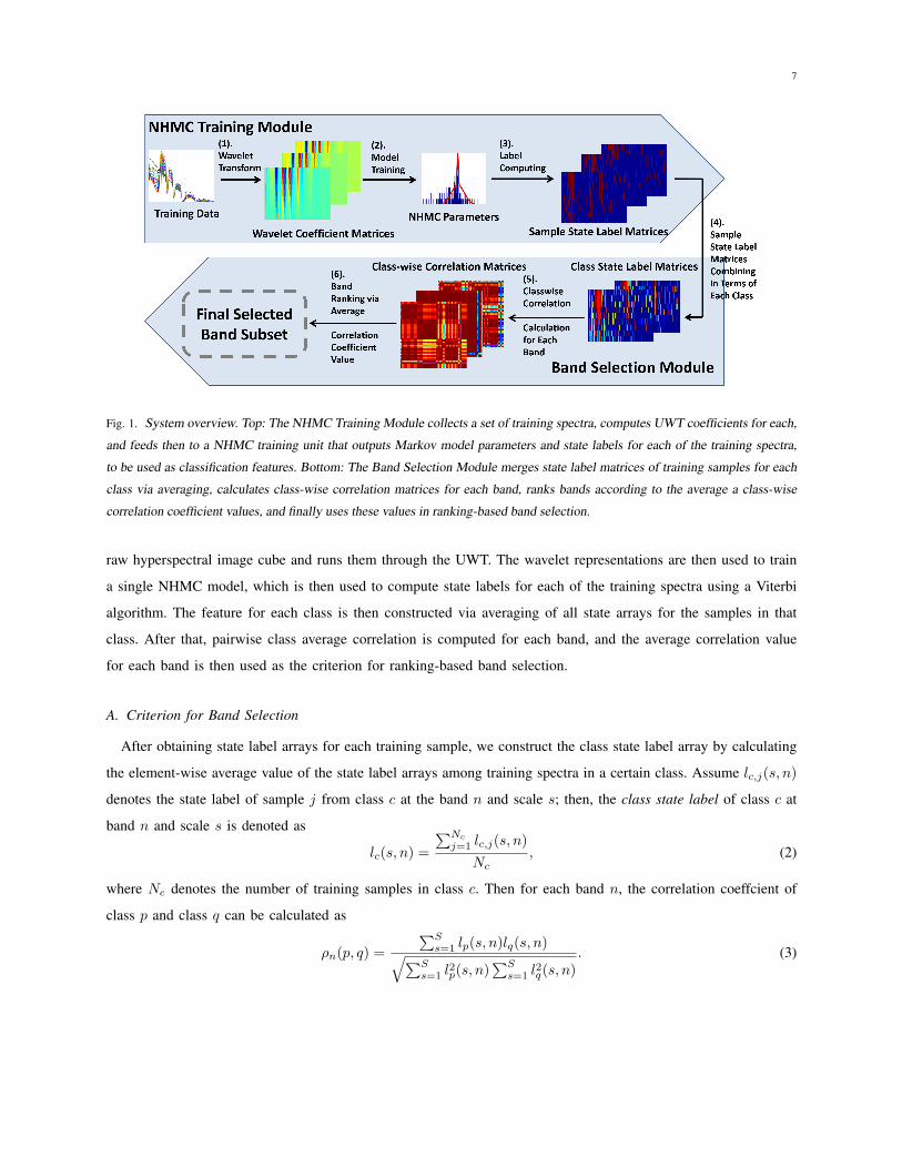
We provide an overview of the NHMC-based band selection procedure in Fig. 1. The system consists of two

modules: an NHMC-based feature training module, and a band selection module. The second module is the

key part of the framework: it assigns rankings to each band and results in the final band subset selection. The

NHMC parameter training stage uses a training library of spectra containing pixels randomly sampled from the

7

Fig. 1. System overview. Top: The NHMC Training Module collects a set of training spectra, computes UWT coefficients for each,

and feeds then to a NHMC training unit that outputs Markov model parameters and state labels for each of the training spectra,

to be used as classification features. Bottom: The Band Selection Module merges state label matrices of training samples for each

class via averaging, calculates class-wise correlation matrices for each band, ranks bands according to the average a class-wise

correlation coefficient values, and finally uses these values in ranking-based band selection.

raw hyperspectral image cube and runs them through the UWT. The wavelet representations are then used to train

a single NHMC model, which is then used to compute state labels for each of the training spectra using a Viterbi

algorithm. The feature for each class is then constructed via averaging of all state arrays for the samples in that

class. After that, pairwise class average correlation is computed for each band, and the average correlation value

for each band is then used as the criterion for ranking-based band selection.

A. Criterion for Band Selection

After obtaining state label arrays for each training sample, we construct the class state label array by calculating

the element-wise average value of the state label arrays among training spectra in a certain class. Assume lc,j(s, n)

denotes the state label of sample j from class c at the band n and scale s; then, the class state label of class c at

band n and scale s is denoted as

lc(s, n) =

∑Nc

j=1 lc,j(s, n)

Nc, (2)

where Nc denotes the number of training samples in class c. Then for each band n, the correlation coeffcient of

class p and class q can be calculated as

ρn(p, q) =

∑Ss=1 lp(s, n)lq(s, n)√∑S

s=1 l2p(s, n)

∑Ss=1 l

2q(s, n)

. (3)

8

The criterion for the ranking of a certain band n is the average of all the pairwise correlation coefficient values for

band n,

Jn =2

C(C − 1)

C−1∑p=1

C∑q=p+1

ρn(p, q), (4)

where C is the number of classes. We then rank the bands in increasing order of correlation (i.e., the band with

lowest correlation is selected first).

B. Multi-State Hidden Markov Chain Model

A two-state zero-mean GMM, as included in an NHMC model, may provide an overly coarse distinction between

sharper absorption bands (fluctuations) and flatter regions in a hyperspectral signature, which are usually assigned

large and small state labels, respectively. In order to investigate the discriminative power of features with finer

characterization of the structural information of hyperspectral signatures, we increase the number of states from 2

to k > 2.

We associate each wavelet coefficient ws with an unobserved hidden state Ss ∈ {0, 1, ..., k−1}, where the states

have prior probabilities pi,s := p(Ss = i) for i = 0, 1, ..., k − 1. Here the state i = 0 represents smooth regions of

the spectral signature, in a fashion similar to the small (S) state for binary GMMs, while i = 1, . . . , k− 1 represent

a more finely grained set of states for spectral signature fluctuations, similarly to the large (L) state in binary

GMMs. All the weights should meet the condition∑k−1

i=0 pi,s = 1. Each state is characterized by a zero-mean

Gaussian distribution for the wavelet coefficient with variance σ2i,s. The value of Ss determines which of the k

components of the mixture model is used to generate the probability distribution for the wavelet coefficient ws:

p(ws|Ss = i) = N (0, σ2i,s). We can then infer that p(ws) =

∑k−1i=0 pi,sp(ws|Ss = i). In analogy with the binary

GMM case, we can also define a k × k transition probability matrix

As =

p0→0,s p1→0,s · · · pk−1→0,s

p0→1,s p1→1,s · · · pk−1→1,s

......

. . ....

p0→k−1,s p1→k−1,s · · · pk−1→k−1,s

,

where pi→j,s = p(Ss = j|Ss−1 = i). Note that the probabilities in the diagonal of As are expected to be larger

than those in the off-diagonal elements due to the persistence property of wavelet transforms. Note also that all

state probabilities pi,s for s > 1 can be derived from the matrices {As}Ls=2 and {pi,1}k−1i=0 .

The training of the k-GMM NHMC is also performed via an EM algorithm. The set of NHMC parameters θn

of a certain spectral band n include the probabilities for the first hidden states {pi,1,n}k−1i=0 , the state transition

matrices {As,n}Ls=2, and the Gaussian variances {σ20,s,n, σ

21,s,n, . . . , σ

2k−1,s,n}Ls=1. In the sequel, we remove from

the parameters θ the dependence on the wavelength index n whenever possible.

C. Redundancy Elimination

In [15], Huang et al. claim that band selection schemes based on band ranking only consider the priority of bands

for a given task, while ignoring the possible redundance between selected bands. Therefore, a redundancy elimination

9

Algorithm 1 Adaptive Band Redundancy Elimination [15]Input: Target number of bands Nb, Ranked band set B, Max. correlation vector V , Threshold updating step δ.

Output: Selected band set S.

1: T = 1

2: S = b1

3: while Size(S) < Nb do

4: T = T − δ

5: for i = 2, i 6 Size(B), i++ do

6: if vi 6 T then

7: S = S ∪ bi8: end if

9: end for

10: end while

11: return S

operation should be performed on ranked bands. However, it is a tradeoff that after redundancy elimination, the

overall relevance of selected bands to the specific problem is inevitably weakened. In Section IV we will verify the

influence of band redundancy elimination on final classification performance.

According to [15], after bands are ranked according to their priorities, the correlation coefficients of each band

(starting from the second band) with all bands before it are calculated. A band will be discarded once its correlation

coefficient with any band before it is greater than a pre-specified threshold T . Final band selection will be conducted

among the remaining bands.

The adaptive band redundancy elimination scheme is described in Algorithm 1. The inputs to this algorithm

include the ranked band set B = {b1, b2, · · · , bN}, where higher ranked bands are listed first, and the maximum

correlation vector V , which is computed as follows. We first compute the pairwise normalized correlation N ×N

matrix D of those ranked bands by calculating band correlation coefficients across the training dataset. More

specifically, di,j represents the normalized correlation value of bands bi and bj . We denote the training dataset by

a matrix X ∈ RN×NT , where NT denotes the cardinality of training set, each column corresponds to a training

data point, and each row corresponds to a spectral band. We can then write

di,j =〈Xbi,:, Xbj ,:〉||Xbi,:‖2‖Xbj ,:||2

(5)

The maximum correlation vector V contains the maximum correlation coefficient values between each band bi and

all bands ranked with higher priority; more specifically, we can write the ith entry of the vector V as

vi = max1≤j<i

di,j , i = 2, 3, · · · , N. (6)

We note that v1 is undefined and is not used in the algorithm.

10

IV. EXPERIMENT AND RESULT ANALYSIS

This section presents the experimental results for the comparison between our proposed method and relevant

tecniques including both pointwise and groupwise band selection.

A. Dateset Description

In order to test the classification performance of the proposed method and four competitors, three different

hyperspectral images were used in the experiment.

1) Kennedy Space Center (KSC). The KSC data, was acquired by NASA AVIRIS (Airborne Visible/Infrared

Imaging Spectrometer) instrument over the Kennedy Space Center (KSC), Florida, on March 23, 1996. The

data corresponds to a hyperspectral image with 224 bands of 10 nm width with center wavelengths from 400

- 2500 nm and a spatial resolution of 18 m. After removing bands with low SNR and corrupted by water

absorption, 176 bands were used in this experiment. The whole image has 512×614 pixels. For classification

purposes, 13 classes were used in this experiment.

2) Botswana. This database was acquired by the NASA EO-1 satellite over the Okavango Delta, Botswana in

2001-2004, which has a spatial resolution of 30 m with 242 bands covering the 400 - 2500 nm spectral range

with spectral resolution of 10 nm. Uncalibrated and noisy bands were removed, and 145 bands remained for

data analysis. The whole image has 1476 × 256 pixels. For classification purposes, 14 classes were used in

this experiment.

3) Whole Indian Pines (WIP). The 92AV3C is a well-known hyperspectral image acquired by AVIRIS with

145 × 145 pixels, 220 spectral bands, and 17 classes, which is a small portion of a larger image known as

Indian Pines. In this experiment, we consider the whole Indian Pines image, which has 2166 × 614 pixels

and 58 classes. However, performing classification on such a large database with a time consuming classifier

(SVM) takes a significant amount of time. We reduce the number of pixels for our simulation by preserving

only those classes containing at least 1000 pixels, and we randomly select 1000 pixels for each of these

classes. Finally, we have removed bands covering the region of water absorption with 200 bands remaining.

For classification purposes, 39 classes were used in this experiment.

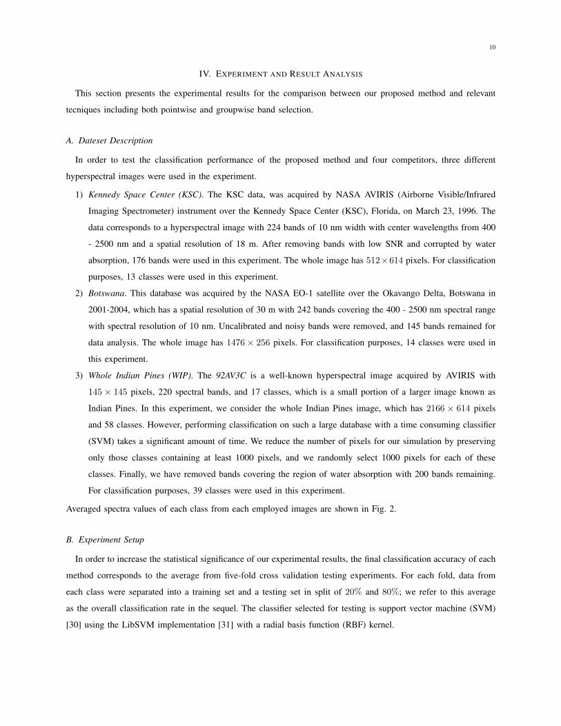
Averaged spectra values of each class from each employed images are shown in Fig. 2.

B. Experiment Setup

In order to increase the statistical significance of our experimental results, the final classification accuracy of each

method corresponds to the average from five-fold cross validation testing experiments. For each fold, data from

each class were separated into a training set and a testing set in split of 20% and 80%; we refer to this average

as the overall classification rate in the sequel. The classifier selected for testing is support vector machine (SVM)

[30] using the LibSVM implementation [31] with a radial basis function (RBF) kernel.

11

20 40 60 80 100 120 1400

0.05

0.1

0.15

0.2

0.25

0.3

0.35

0.4

0.45

0.5

Band Number

Reflecta

nce

(a) Botswana

20 40 60 80 100 120 140 1600

0.005

0.01

0.015

0.02

0.025

0.03

0.035

Band Number

Reflecta

nce

(b) KSC

20 40 60 80 100 120 140 160 180 2000

0.1

0.2

0.3

0.4

0.5

0.6

0.7

Band Number

Re

fle

cta

nce

(c) WIP

Fig. 2. Average spectra for each class present in each image for the three images used in the experiments.

5 20 35 50 65 80 95 110 125 140

86

87

88

89

90

91

92

93

94

Number of Bands Selected

Overa

ll C

lassific

ation A

ccura

cy / %

3 5 6 6 6 6 7 7 7 7 7 7 3 2 2 2 2 6 6 2 2 4 7 6 6 6 6 6

NHMCMEACMIFWRelief−FAll Bands0.99 Line

(a) Botswana

5 20 35 50 65 80 95 110 125 140 155 170

88

89

90

91

92

93

94

Number of Bands Selected

Overa

ll C

lassific

ation A

ccura

cy / %

6522555222588677887777777778863334

NHMCMEACMIFWRelief−FAll Bands0.99 Line

(b) KSC

10 20 30 40 50 60 70 80 90 100 110 120 130 140 150 160 17040

45

50

55

60

Number of Bands Selected

Overa

ll C

lassific

ation A

ccura

cy / %

4 4 5 5 5 4 4 4 4 4 6 8 8 8 8 8 8

NHMCMEACMIFWRelief−FAll Bands0.99 Line

(c) WIP

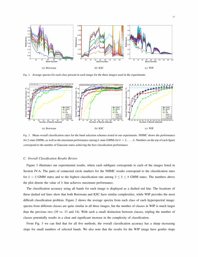
Fig. 3. Mean overall classification rates for the band selection schemes tested in our experiments. NHMC shows the performance

for 2-state GMMs, as well as the maximum performance among k-state GMMs for k = 2, . . . , 8. Numbers on the top of each figure

correspond to the number of Gaussian states achieving the best classification performance.

C. Overall Classification Results Review

Figure 3 illustrates our experimental results, where each subfigure corresponds to each of the images listed in

Section IV-A. The pairs of connected circle markers for the NHMC results correspond to the classification rates

for k = 2 GMM states and to the highest classification rate among 2 ≤ k ≤ 8 GMM states. The numbers above

the plot denote the value of k that achieves maximum performance.

The classification accuracy using all bands for each image is displayed as a dashed red line. The locations of

these dashed red lines show that both Botswana and KSC have similar complexities, while WIP provides the most

difficult classification problem. Figure 2 shows the average spectra from each class of each hyperspectral image:

spectra from different classes are quite similar in all three images, but the number of classes in WIP is much larger

than the previous two (39 vs. 13 and 14). With such a small distinction between classes, tripling the number of

classes potentially results in a clear and significant increase in the complexity of classification.

From Fig. 3 we can find that for all five methods, the overall classification accuracy has a sharp increasing

slope for small numbers of selected bands. We also note that the results for the WIP image have gentler slope

12

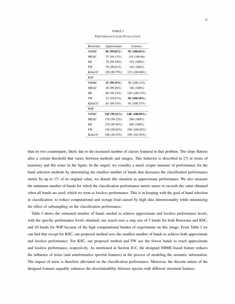
TABLE I

PERFORMANCE LOSS EVALUATION

Botswana Approximate Lossless

NHMC 30 (99.02%) 70 (100.03%)

MEAC 35 (99.11%) 110 (100.06)

MI 70 (99.10%) 145 (100%)

FW 70 (99.01%) 145 (100%)

Relief-F 120 (99.79%) 135 (100.06%)

KSC

NHMC 15 (99.19%) 50 (100.11%)

MEAC 40 (99.26%) 146 (100%)

MI 80 (99.12%) 120 (100.15%)

FW 25 (99.67%) 30 (100.10%)

Relief-F 65 (99.35%) 95 (100.37%)

WIP

NHMC 120 (99.21%) 140 (100.09%)

MEAC 170 (99.12%) 200 (100%)

MI 170 (99.56%) 200 (100%)

FW 150 (99.02%) 190 (100.02%)

Relief-F 180 (99.35%) 190 (101.85%)

than its two counterparts, likely due to the increased number of classes featured in that problem. The slope flattens

after a certain threshold that varies between methods and images. This behavior is described in [7] in terms of

transitory and flat zones in the figure. In the sequel, we consider a much crisper measure of performance for the

band selection methods by determining the smallest number of bands that decreases the classification performance

metric by up to 1% of its original value; we denote this situation as approximate performance. We also measure

the minimum number of bands for which the classification performance metric meets or exceeds the value obtained

when all bands are used, which we term as lossless performance. This is in keeping with the goal of band selection

in classification: to reduce computational and storage load caused by high data dimensionality while minimizing

the effect of subsampling on the classification performance.

Table I shows the estimated number of bands needed to achieve approximate and lossless performance levels,

with the specific performance levels obtained; our search uses a step size of 5 bands for both Botswana and KSC,

and 10 bands for WIP because of the high computational burden of experiments on this image. From Table I we

can find that except for KSC, our proposed method uses the smallest number of bands to achieve both approximate

and lossless performance. For KSC, our proposed method and FW use the fewest bands to reach approximate

and lossless performance, respectively. As mentioned in Section II-C, the designed NHMC-based feature reduces

the influence of noise (and uninformative spectral features) in the process of modeling the semantic information.

The impact of noise is therefore alleviated on the classification performance. Moreover, the discrete nature of the

designed features arguably enhances the discriminability between spectra with different structural features.

13

We observe that most methods are able to achieve higher classification rates with band selection than when using

all bands. However, there are two reasons why these advantages in classification rates of band selection methods

being not emphasized in this paper. First, in most cases the band numbers needed for improved classification

performance are too large to enable the computational load reduction that motivates band selection. Second, in all

three tested images, none of the tested methods achieved a classification rate greater than 1% above that of using

all bands. This means that such advantages are negligible.

D. Effect of Multi-State Gaussian Mixtures

Recall that Section III-B argued for increasing the number of states in the GMM so improve the discriminability

of the obtained label-based feature between different spectra. From Fig. 3, we can find that for most cases in

Botswana and WIP, multi-state GMM achieves better performance than binary-state GMM. However, the advantage

of multi-state GMM is usually less than 1%. Only in the case of 5 selected bands in Botswana and 40 selected

bands in WIP, multi-state GMM achieves classification rates more than 2% higher than binary-state GMM. For KSC,

binary-state GMM provides the best performance in several cases. After analyzing the variance of classification

rates for different numbers of GMM states at each selected band size, we found that for both Botswana and KSC,

the largest variance values appear at 5 bands, and for WIP the largest value appears in 40 bands. In other words,

largest variance in each image appears in the case of least selected bands. According to our observation, the specific

choice of selected bands appears to be more diverse with small band size. So the relatively large advantages of

multi-state GMM happening at those band sizes is more likely to be a result of the large diversity of classification

rates than the model themselves. We will discuss this behavior in more detail in Section IV-E.

Although a large number of GMM states captures more structural information in hyperspectral data, it might

also have a negative influence on the classification results. First, the GMM state of a particular wavelet coefficient

ws,n is determined by the coefficient’s magnitude with respect to those for the rest of the NHMC training spectra,

the state label of its parent Ss−1,n, and the transition probability matrix As,n. In practice, such dependence causes

different maps between coefficient value ranges and GMM states across scales and offsets (s, n). The variance

often makes it difficult to assess the semantic information in the label array of a spectral signature. In practice,

this variance may sometimes affect the interpretability of features obtained from GMM labels. Furthermore, the

likelihood of such variability in the value-to-state mappings could increase when more states are used. Second,

when more states are introduced, the likelihood of fine-scale coefficients being labeled as large/significance also

increases. Therefore, the classification performance may be more sensitive to noise.

E. Impact of Redundancy Elimination

Next, we test the effect of redundancy elimination (cf. Section III-C) in band selection performance. Due to the

diversity of statistics in different training sets, we determine the threshold of redundancy elimination adaptively for

each data set by fixing the number of bands remaining after redundancy elimination, which is denoted as Nb. For

adaptive band redundancy elimination (Algorithm 1), we choose Nb = 20 and δ = 0.001.

14

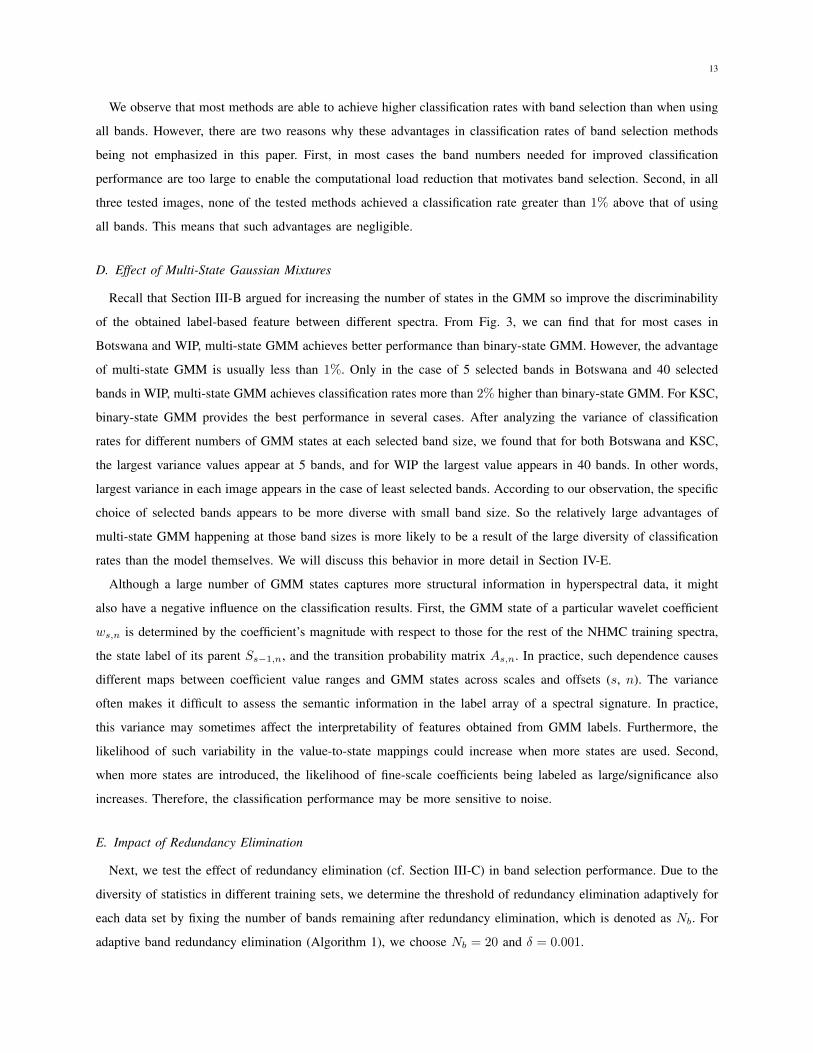
TABLE II

COMPARISON OF CLASSIFICATION PERFORMANCE BEFORE AND AFTER REDUNDANCY ELIMINATION

Botswana 5 Bands 10 Bands 15 Bands 20 Bands

NHMC 85.87% 89.09% 90.71% 91.59% 91.90% 91.71% 92.83% 91.51%

MI 79.59% 79.86% 84.84% 87.41% 86.64% 90.02% 88.98% 90.25%

FW 84.97% 85.35% 88.00% 90.37% 90.98% 91.16% 91.59% 92.06%

Relief-F 62.57% 84.68% 79.33% 86.21% 84.24% 91.03% 86.54% 91.74%

KSC

NHMC 87.26% 87.34% 91.84% 90.27% 93.01% 90.67% 93.20% 90.76%

MI 53.58% 49.37% 63.33% 83.06% 71.87% 88.37% 77.08% 87.19%

FW 88.58% 88.03% 91.40% 91.45% 92.41% 91.33% 92.72% 90.39%

Relief-F 73.74% 90.33% 80.62% 92.22% 85.08% 91.83% 86.94% 91.34%

WIP

NHMC 31.01% 39.23% 40.08% 47.25% 46.38% 44.92% 48.97% 45.44%

MI 18.48% 11.82% 22.02% 32.28% 26.96% 35.11% 39.28% 36.66%

FW 35.42% 40.15% 46.66% 44.10% 49.42% 44.68% 52.64% 44.02%

Relief-F 21.79% 39.10% 24.66% 44.24% 26.22% 46.35% 31.85% 44.32%

20 40 60 80 100 120 140

1

2

3

4

5

Band Number

Cro

ss V

alid

atio

n F

old

ID

(a) 5 Bands

20 40 60 80 100 120 140

1

2

3

4

5

Band Number

Cro

ss V

alid

atio

n F

old

ID

(b) 15 Bands

20 40 60 80 100 120 140

1

2

3

4

5

Band Number

Cro

ss V

alid

atio

n F

old

ID

(c) 5 Bands

20 40 60 80 100 120 140

1

2

3

4

5

Band NumberC

ross V

alidation F

old

ID

(d) 15 Bands

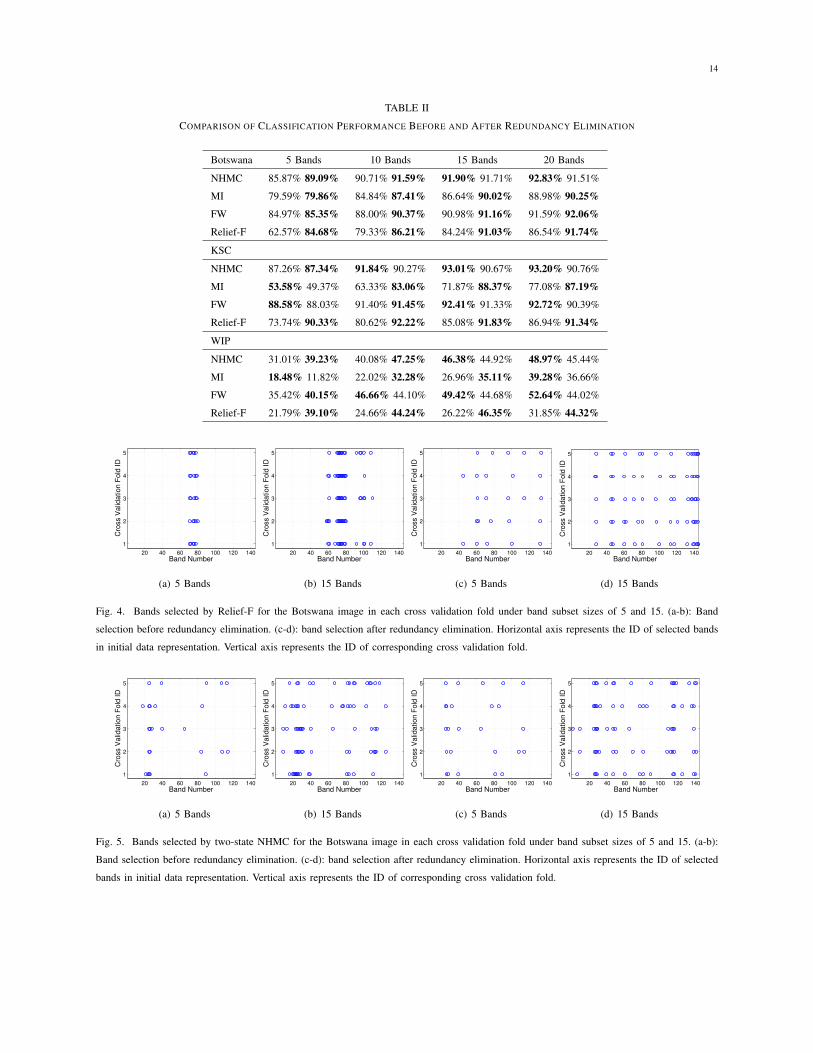
Fig. 4. Bands selected by Relief-F for the Botswana image in each cross validation fold under band subset sizes of 5 and 15. (a-b): Band

selection before redundancy elimination. (c-d): band selection after redundancy elimination. Horizontal axis represents the ID of selected bands

in initial data representation. Vertical axis represents the ID of corresponding cross validation fold.

20 40 60 80 100 120 140

1

2

3

4

5

Band Number

Cro

ss V

alid

atio

n F

old

ID

(a) 5 Bands

20 40 60 80 100 120 140

1

2

3

4

5

Band Number

Cro

ss V

alid

atio

n F

old

ID

(b) 15 Bands

20 40 60 80 100 120 140

1

2

3

4

5

Band Number

Cro

ss V

alid

atio

n F

old

ID

(c) 5 Bands

20 40 60 80 100 120 140

1

2

3

4

5

Band Number

Cro

ss V

alid

atio

n F

old

ID

(d) 15 Bands

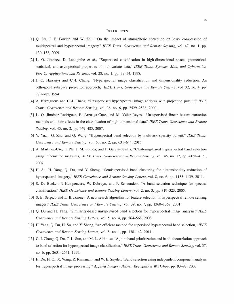
Fig. 5. Bands selected by two-state NHMC for the Botswana image in each cross validation fold under band subset sizes of 5 and 15. (a-b):

Band selection before redundancy elimination. (c-d): band selection after redundancy elimination. Horizontal axis represents the ID of selected

bands in initial data representation. Vertical axis represents the ID of corresponding cross validation fold.

15

Our experiment compares the classification performance for the bands selected with and without redundancy

elimination for each band selection scheme. We let Nb = 5, 10, 15, and 20; the classification performance results

are listed in Table II. The higher classification rate (either with or without redundancy elimination) in each case

is highlighted by boldface. The table shows that redundancy elimination improves classification performance in

more than half of all cases, especially for Relief-F. To illustrate the diversity of features selected with and without

redundancy elimination, Fig. 4 shows the distributions of the selected bands before and after redundancy elimination

using Relief-F. It is apparent that redundancy elimination greatly improves the diversity in band distribution in this

case. Because of the high correlation between nearby bands in hyperspectral images, selecting bands from a wider,

more diverse distribution makes the selected bands more representative of the overall structure of a hyperspectral

image (and therefore more informative). From Table II, we see that redundancy elimination improves classification

rates in most cases. However, we also note that redundancy elimination does not bring significant improvement in

classification performance for NHMC. By using the same setup as in Fig. 4, we plot the band distribution of NHMC

with 2 GMM states in Fig. 5. The figure shows that the selected bands before redundancy elimination are already

quite diverse, and redundancy elimination does not seem to improve this aspect further. In addition, for large values

of Nb, such as 15 and 20, redundancy elimination even appears to have negative influence on the classification

performance. That is because with the increase in band set size, more bands with low priority are included, which

may generate negative influence on the classification accuracy. Although we only considered Nb ≤ 20 for brevity,

it is reasonable to expect that any performance losses vanish as Nb grows larger.

V. CONCLUSION

We propose a supervised band selection framework that reduces redundancy in hyperspectral image bands while

preserving useful semantic information. The proposed scheme uses a non-homogeneous hidden Markov chain

(NHMC) model in conjunction with an undecimated wavelet transform to design features capturing the semantic

information in the structure of each single-pixel hyperspectral datum while reducing the effect of noise. A band

selection criterion is constructed based on class-wide features, aiming to minimize the correlation between the

obtained class-wide features. The obtained experimental results demonstrate the advantages of our method over

other relevant techniques. In addition, we also tested the influence brought by increased GMM state number and

impacts of redundancy elimination. The results tell us the eligibility of a simple GMM and the necessity of a high

band diversity.

In the future, we will focus on the fusion of band selection and spatial information in hyperspectral classification

problems. Additionally, the extension to unsupervised band selection will also be considered.

ACKNOWLEDGMENT

We thank Mr. Ping Fung for providing an efficient implementation of our NHMC training code that largely

decreased the time of running experiments.

16

REFERENCES

[1] Q. Du, J. E. Fowler, and W. Zhu, “On the impact of atmospheric correction on lossy compression of

multispectral and hyperspectral imagery,” IEEE Trans. Geoscience and Remote Sensing, vol. 47, no. 1, pp.

130–132, 2009.

[2] L. O. Jimenez, D. Landgrebe et al., “Supervised classification in high-dimensional space: geometrical,

statistical, and asymptotical properties of multivariate data,” IEEE Trans. Systems, Man, and Cybernetics,

Part C: Applications and Reviews, vol. 28, no. 1, pp. 39–54, 1998.

[3] J. C. Harsanyi and C.-I. Chang, “Hyperspectral image classification and dimensionality reduction: An

orthogonal subspace projection approach,” IEEE Trans. Geoscience and Remote Sensing, vol. 32, no. 4, pp.

779–785, 1994.

[4] A. Ifarraguerri and C.-I. Chang, “Unsupervised hyperspectral image analysis with projection pursuit,” IEEE

Trans. Geoscience and Remote Sensing, vol. 38, no. 6, pp. 2529–2538, 2000.

[5] L. O. Jimenez-Rodrıguez, E. Arzuaga-Cruz, and M. Velez-Reyes, “Unsupervised linear feature-extraction

methods and their effects in the classification of high-dimensional data,” IEEE Trans. Geoscience and Remote

Sensing, vol. 45, no. 2, pp. 469–483, 2007.

[6] Y. Yuan, G. Zhu, and Q. Wang, “Hyperspectral band selection by multitask sparsity pursuit,” IEEE Trans.

Geoscience and Remote Sensing, vol. 53, no. 2, pp. 631–644, 2015.

[7] A. Martınez-Uso, F. Pla, J. M. Sotoca, and P. Garcıa-Sevilla, “Clustering-based hyperspectral band selection

using information measures,” IEEE Trans. Geoscience and Remote Sensing, vol. 45, no. 12, pp. 4158–4171,

2007.

[8] H. Su, H. Yang, Q. Du, and Y. Sheng, “Semisupervised band clustering for dimensionality reduction of

hyperspectral imagery,” IEEE Geoscience and Remote Sensing Letters, vol. 8, no. 6, pp. 1135–1139, 2011.

[9] S. De Backer, P. Kempeneers, W. Debruyn, and P. Scheunders, “A band selection technique for spectral

classification,” IEEE Geoscience and Remote Sensing Letters, vol. 2, no. 3, pp. 319–323, 2005.

[10] S. B. Serpico and L. Bruzzone, “A new search algorithm for feature selection in hyperspectral remote sensing

images,” IEEE Trans. Geoscience and Remote Sensing, vol. 39, no. 7, pp. 1360–1367, 2001.

[11] Q. Du and H. Yang, “Similarity-based unsupervised band selection for hyperspectral image analysis,” IEEE

Geoscience and Remote Sensing Letters, vol. 5, no. 4, pp. 564–568, 2008.

[12] H. Yang, Q. Du, H. Su, and Y. Sheng, “An efficient method for supervised hyperspectral band selection,” IEEE

Geoscience and Remote Sensing Letters, vol. 8, no. 1, pp. 138–142, 2011.

[13] C.-I. Chang, Q. Du, T.-L. Sun, and M. L. Althouse, “A joint band prioritization and band-decorrelation approach

to band selection for hyperspectral image classification,” IEEE Trans. Geoscience and Remote Sensing, vol. 37,

no. 6, pp. 2631–2641, 1999.

[14] H. Du, H. Qi, X. Wang, R. Ramanath, and W. E. Snyder, “Band selection using independent component analysis

for hyperspectral image processing,” Applied Imagery Pattern Recognition Workshop, pp. 93–98, 2003.

17

[15] R. Huang and M. He, “Band selection based on feature weighting for classification of hyperspectral data,”

IEEE Geoscience and Remote Sensing Letters, vol. 2, no. 2, pp. 156–159, 2005.

[16] L. Chen, R. Huang, and W. Huang, “Graph-based semi-supervised weighted band selection for classification of

hyperspectral data,” in IEEE Int. Conf. Audio Language and Image Processing (ICALIP), 2010, pp. 1123–1126.

[17] S. Murchie, R. Arvidson, P. Bedini, K. Beisser, J.-P. Bibring, J. Bishop, J. Boldt, P. Cavender, T. Choo,

R. Clancy et al., “Compact reconnaissance imaging spectrometer for Mars (CRISM) on Mars reconnaissance

orbiter (MRO),” Journal of Geophysical Research: Planets, vol. 112, no. E5, 2007.

[18] B. Guo, S. R. Gunn, R. Damper, and J. Nelson, “Band selection for hyperspectral image classification using

mutual information,” IEEE Geoscience and Remote Sensing Letters, vol. 3, no. 4, pp. 522–526, 2006.

[19] S. Feng, Y. Itoh, M. Parente, and M. F. Duarte, “Tailoring non-homogeneous Markov chain wavelet models for

hyperspectral signature classification,” in IEEE Int. Conf. Image Processing (ICIP), Paris, France, Oct. 2014.

[20] ——, “Wavelet-based semantic features for hyperspectral signature discrimination,” Apr. 2015, Available at

http://arxiv.org/abs/1602.03903.

[21] S. Mallat, A wavelet tour of signal processing. San Diego, CA: Academic Press, 1999.

[22] S. Mallat and W. Hwang, “Singularity detection and processing with wavelets,” IEEE Trans. Information

Theory, vol. 38, no. 2, pp. 617–643, Mar. 1992.

[23] S. Mallat and S. Zhong, “Characterization of signals from multiscale edges,” IEEE Trans. Pattern Analysis

and Machine Intelligence, vol. 14, no. 7, pp. 710–732, Jul. 1992.

[24] M. T. Orchard and K. Ramchandran, “An investigation of wavelet-based image coding using an engropy-

constrained quantization framework,” in Data Compression Conf. (DCC), Snowbird, UT, Mar. 1994, pp. 341–

350.

[25] L. R. Rabiner, “A tutorial on hidden Markov models and selected applications in speech recognition,”

Proceedings of the IEEE, vol. 77, no. 2, pp. 257–286, 1989.

[26] S. Prasad, W. Li, J. E. Fowler, and L. M. Bruce, “Information fusion in the redundant-wavelet-transform

domain for noise-robust hyperspectral classification,” IEEE Trans. Geoscience and Remote Sensing, vol. 50,

no. 9, pp. 33 473–3486, 2012.

[27] K. Kira and L. A. Rendell, “The feature selection problem: Traditional methods and a new algorithm,” in

National Conf. Artificial Intelligence (AAAI), vol. 2, 1992, pp. 129–134.

[28] I. Kononenko, “Estimating attributes: analysis and extensions of RELIEF,” in Machine Learning: European

Conf. Machine Learning (ECML)-94. Springer, 1994, pp. 171–182.

[29] T. M. Cover and J. A. Thomas, Elements of Information Theory. New York, NY, USA: Wiley-Interscience,

2006.

[30] N. Cristianini and J. Shawe-Taylor, An introduction to support vector machines and other kernel-based learning

methods. Cambridge university press, 2000.

[31] C.-C. Chang and C.-J. Lin, “LibSVM: A library for support vector machines,” ACM Trans. Intelligent Systems

and Technology, vol. 2, no. 3, p. 27, 2011.