Statistical Inference After Model Selectionlbrown/Papers/2009a...Statistical Inference After Model Selection Richard Berk Department of Statistics Department of Criminology University

Statistical Inference After Model Selection∗

Richard BerkDepartment of Statistics

Department of CriminologyUniversity of Pennsylvania

([email protected])

Lawrence BrownLinda Zhao

Department of StatisticsUniversity of Pennsylvania

September 15, 2009

Abstract

Conventional statistical inference requires that a model of how thedata were generated be known before the data are analyzed. Yet incriminology, and in the social sciences more broadly, a variety of modelselection procedures are routinely undertaken followed by statisticaltests and confidence intervals computed for a “final” model. In thispaper, we examine such practices and show how they are typicallymisguided. The parameters being estimated are no longer well de-fined, and post-model-selection sampling distributions are mixtures

∗Richard Berk’s work on this paper was funded by a grant from the National ScienceFoundation: SES-0437169, “Ensemble methods for Data Analysis in the Behavioral, Socialand Economic Sciences.” The work by Lawrence Brown and Linda Zhao was support inpart by NSF grant DMS-07-07033. Thanks also go to Andreas Buja, Sam Preston, JasjeetSekhon, Herb Smith, Phillip Stark, and three reviewers for helpful suggestions about thematerial discussed in this paper.

1

with properties that are very different from what is conventionallyassumed. Confidence intervals and statistical tests do not performas they should. We examine in some detail the specific mechanismsresponsible. We also offer some suggestions for better practice andshow though a criminal justice example using real data how properstatistical inference in principle may be obtained.

1 Introduction

In textbook treatments of regression analysis, a model is a theory of how thedata on hand were generated. Regressors are canonically treated as fixed,and the model specifies how the realized distribution of the response variablecame to be, given the values of the regressors (Freedman, 2005: 42). Causalinterpretations can be introduced from information external to the model(Berk, 2003: Chapter 5). Statistical tests and confidence intervals can beconstructed.

This basic framework subsumes a variety of special cases. Popular in-stances are included under the generalized linear model and its extensions(McCullagh and Nelder, 1989). Logistic regression is common example. Mod-els with more than one regression equation (Greene, 2003: Chapters 14 and15) are for purposes of this paper also special cases.

The ubiquitous application of regression models in criminology, and inthe social sciences more generally, has been criticized from a variety of per-spectives for well over a generation (Box, 1976; Leamer, 1978; Rubin, 1986;Freedman, 1987; 2004; Manski, 1990; Breiman, 2001; Berk, 2003; Morganand Winship, 2007). Despite the real merits of this literature, we assumein this paper that the idea of a “correct model” makes sense and considerstatistical inference when the correct model is not known before the data areanalyzed. We proceed, therefore, consistent with much common practice.

Statistical inference for regression assumes that there is a correct modelthat accurately characterizes the data generation process. This model isknown, except for the values of certain parameters, before the data are ex-amined (Freedman, 2005: 64-65). The same holds for statistical inferencemore generally (Barnett, 1982: Section 5.1).1 Consequently, arriving at one

1“Thus sample data, x, are assumed to arise from observing a random variable Xdefined on a sample space, <. The random variable X has a probability distributionpθ(x) which is assumed known except for the value of the parameter Θ. The parameter Θ

2

or more regression models through data analysis would seem to make sub-sequent statistical inference problematic. Yet, model selection is a routineactivity and is taught in any number of respected textbooks (Cook and Weis-berg, 1999, Greene, 2003). This practice and pedagogy, therefore, would seemto warrant some scrutiny. Is there a problem? If so, is it important? And ifso, what can be done about it? What are the consequences, for instance, ofdeleting “insignificant” predictors from a regression equation, re-estimatingthe model’s parameter values, and applying statistical tests to the “final”model?

In the pages ahead, we show that when data used to arrive at one ormore regression models are also used to estimate the values of model pa-rameters and to conduct statistical tests or construct confidence intervals,the sampling distributions on which proper estimates, statistical tests andconfidence intervals depend can be badly compromised. It follows that theparameters estimates, statistical tests and confidence intervals can be badlycompromised a well. Moreover, because the compromised sampling distri-butions depend on complex interactions between a suite of possible modelsand the data to be analyzed, inferential errors are typically very difficult toidentify and correct. It is far better, therefore, to avoid the problems to beginwith. We suggest several ways by which this can be done.

In section 2, the difficulties with “post-model-selection” statistical infer-ence are introduced. Section 3 considers the particular mechanisms by whichmodel selection can undermine statistical inference. To our knowledge, thisdiscussion is novel. Section 4 illustrates through simulations the kinds ofdistortions that can result. Section 5 discusses some potential remedies andshows with real data one example of appropriate practice. Section 6 drawssome overall conclusions.

2 Framing the Problem of Post-Model-Selection

Statistical Inference

When in a regression analysis the correct model is unknown before the dataare introduced, researchers will often proceed in four steps.

is some member of a specified parameter space Ω; x (and the random variable X) andΘ may have one or many components” (Barnett, 1982: 121). Emphasis in the original.Some minor changes in notation have been made.

3

1. A set of models is constructed.

2. The data are examined, and a “final” model is selected.

3. The parameters of that model are estimated.

4. Statistical inference is applied to the parameter estimates.

Criminologists are certainly no exception. Davies and Dedel (2006), for in-stance, develop a violence risk screening instrument to be used in communitycorrections settings by reducing a logistic regression model with nine regres-sors to a logistic regression model with three regressors. Wald tests areapplied to regression coefficients of the three-regressor model.

In many crime and justice analyses, some of the steps can be combinedand are typically more complicated when there is more than one “final”model. For example, Ousey, Wilcox and Brummel (2008), consider whethera criminal victimization changes the likelihood of subsequent victimizations.Several competing models are developed. Some are discarded because of un-satisfactory statistical and interpretative properties. A variety of statisticaltests are applied to each model, including the preferred ones. Lalond andCho (2008), undertake a similar exercise for the impact of incarcerations onfemale inmates’ employment prospects. There are both statistical and sub-stantive considerations that lead the authors to favor some of their modelsover others, and there is a liberal use of statistical tests. Schroeder, Gior-dano, and Cernkovich (2007) consider the relative impact of drug and alcoholuse on crime desistance by constructing a large number of competing models,some of which are deemed more instructive than others. Again, there is aliberal use of statistical tests, including for the models taken to be most in-structive. Sampson and Raudenbush (2004) examine the causes of perceivedneighborhood disorder through several different models, some of which arediscarded for spurious associations. Conventional t-tests are used for all ofthe models including the subset of preferable models on which the substan-tive conclusions rest. In short, post-model-selection statistical inference is aroutine activity in crime and justice research.

Each of the four steps can individually be legitimate. The problems ad-dressed in this paper occur when all four steps are undertaken with the samedata set. Perhaps the most apparent difficulty is that the model selectionprocess in the first step is a form of data snooping. Standard errors conven-tionally estimated under such circumstances are well know to be incorrect;

4

they are likely to too small (Freedman et al., 1988). False statistical powercan result. In effect, there is an opportunity to look at all the face-down cardsbefore a bet is placed.2 For most thoughtful crime and justice researchers,this is old news.

The problems addressed here are more fundamental. It has long beenrecognized by some that when any parameter estimates are discarded, thesampling distribution of the remaining parameter estimates can be distorted.(Brown, 1967; Olshen, 1973). The rules by which some parameters are dis-carded do not even have to exploit information from the data being analyzed.The rules may be “ancillary” in the sense that they are constructed indepen-dently of the parameters responsible for the realized data (Brown, 1990:489).3

For example, suppose the model a researcher selects depends on the dayof the week. On Mondays it’s model A, on Tuesdays it’s model B, and so onup to seven different models on seven different days. Each model, therefore,is the “final” model with a probability of 1/7th that has nothing to do withthe values of the regression parameters. Then, if the data analysis happens tobe done on a Thursday, say, it is the results from model D that are reported.All of the other model results that could have been reported are not. Thoseparameter estimates are summarily discarded.

Distorted sampling distributions of the sort discussed in the pages aheadcan materialize under ancillary selection rules. It is the exclusion of certainestimates by itself that does the damage. In practice, however, the selectionrule will not likely be ancillary; it will be dependent on regression parame-ters. For example, the selection rule may favor models with smaller residualvariances.

Recent work has rediscovered and extended these insights while focussingparticularly on the regression case. Leeb and Potscher (2006; 2008) showthat the sampling distributions of post-model-selection parameter estimatesare likely to be unknown, and probably unknowable, even asymptotically.Moreover, it does not seem to matter what kind of model selection approach

2There are also the well-known difficulties that can follow from undertaking a largenumber of statistical tests. With every 20 statistical tests a researcher undertakes, forexample, one null hypothesis will on the average be rejected at the .05 level even if allthe null hypothesis are true. Remedies for the multiplicity problem are currently a livelyresearch area in statistics (e.g., Benjamini and Yekutieli, 2001; Efron, 2007).

3The context in which Brown is working is rather different from the present context.But the same basic principles apply.

5

is used. Informal data exploration and tinkering produces the same kindsof difficulties as automated procedures in which the researcher does not par-ticipate except at the very beginning and the very end. Judgment-basedmodel selection is in this sense no different from nested testing, stepwiseregression, all subsets regression, shrinkage estimators (Efron et al., 2007),the Dantzig Selector (Candes and Tao, 2007), and all other model selectionmethods considered to date (Leeb and Potscher, 2005). Likewise, the par-ticular screening statistic applied is immaterial: an adjusted R2, AIC, BIC,Mallows’ Cp, cross-validiation, p-values or others (Leeb and Potscher, 2005).

3 A More Formal Treatment

The conceptual apparatus in which frequentist statistical inference is placedimagines a limitless number of independent probability samples drawn froma well-defined population. From each sample, one or more sample statisticsare computed. The distribution of each sample statistic, over samples, isthe sampling distribution for that sample statistic. Statistical inference isundertaken from these sampling distributions. To take a common textbookillustration, the sample statistic is a mean. A sampling distribution for themean is the basis for any confidence intervals or a statistical test that fol-low. The same framework applies to the parameters of a regression equationwhen the structure of the regression equation is known before the data areanalyzed.4

3.1 Definitional Problems

Past discussions of post-model-selection statistical inference have apparentlynot recognized that when the regression model is not fully specified before thedata are examined, important definitional ambiguities are introduced. Any

4There is an alternative formulation that mathematically amounts to the same thing.In the real world, nature generates the data through a stochastic process characterizedby a regression model. Inferences are made to the parameters of this model, not to theparameters of a regression in a well-defined population. Data on hand are not a randomsample from that population, but are a random realization of a stochastic process, andthere can be a limitless number of independent realizations. These two formulations andothers are discussed in far more detail elsewhere (Berk, 2004: 39-58). The material tofollow is effectively the same under either account, but the random sampling approach isless abstract and easier build upon.

6

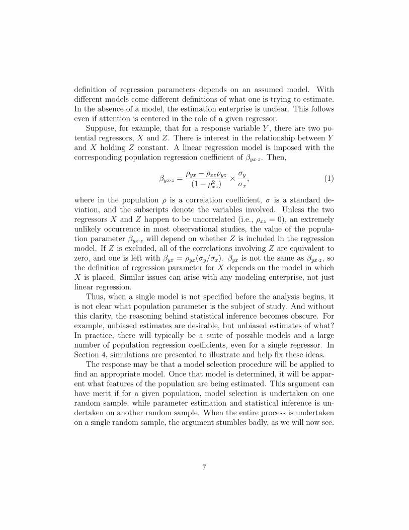
definition of regression parameters depends on an assumed model. Withdifferent models come different definitions of what one is trying to estimate.In the absence of a model, the estimation enterprise is unclear. This followseven if attention is centered in the role of a given regressor.

Suppose, for example, that for a response variable Y , there are two po-tential regressors, X and Z. There is interest in the relationship between Yand X holding Z constant. A linear regression model is imposed with thecorresponding population regression coefficient of βyx·z. Then,

βyx·z =ρyx − ρxzρyz

(1− ρ2xz)

× σy

σx

, (1)

where in the population ρ is a correlation coefficient, σ is a standard de-viation, and the subscripts denote the variables involved. Unless the tworegressors X and Z happen to be uncorrelated (i.e., ρxz = 0), an extremelyunlikely occurrence in most observational studies, the value of the popula-tion parameter βyx·z will depend on whether Z is included in the regressionmodel. If Z is excluded, all of the correlations involving Z are equivalent tozero, and one is left with βyx = ρyx(σy/σx). βyx is not the same as βyx·z, sothe definition of regression parameter for X depends on the model in whichX is placed. Similar issues can arise with any modeling enterprise, not justlinear regression.

Thus, when a single model is not specified before the analysis begins, itis not clear what population parameter is the subject of study. And withoutthis clarity, the reasoning behind statistical inference becomes obscure. Forexample, unbiased estimates are desirable, but unbiased estimates of what?In practice, there will typically be a suite of possible models and a largenumber of population regression coefficients, even for a single regressor. InSection 4, simulations are presented to illustrate and help fix these ideas.

The response may be that a model selection procedure will be applied tofind an appropriate model. Once that model is determined, it will be appar-ent what features of the population are being estimated. This argument canhave merit if for a given population, model selection is undertaken on onerandom sample, while parameter estimation and statistical inference is un-dertaken on another random sample. When the entire process is undertakenon a single random sample, the argument stumbles badly, as we will now see.

7

PopulationM1

M2

M3

M2

M4

M5

M2

M1

M6

Realized Models Over Samples

Ω1

Ω2

Ω3

Ω2

Ω4

Ω5

Ω2

Ω1

Ω6ˆ

ˆ

ˆ

ˆ

ˆˆ

ˆ

ˆ

ˆˆ

ˆ

ˆ

ˆˆ

ˆ

ˆ

ˆ

ˆ

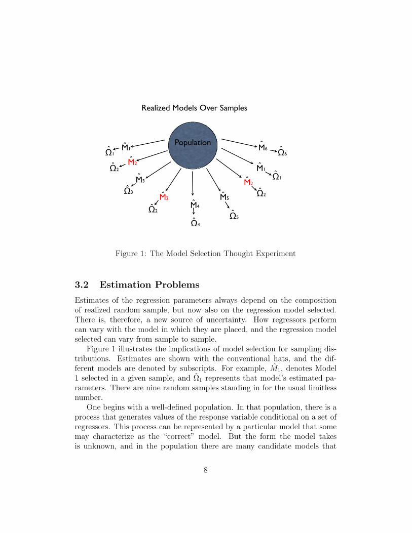
Figure 1: The Model Selection Thought Experiment

3.2 Estimation Problems

Estimates of the regression parameters always depend on the compositionof realized random sample, but now also on the regression model selected.There is, therefore, a new source of uncertainty. How regressors performcan vary with the model in which they are placed, and the regression modelselected can vary from sample to sample.

Figure 1 illustrates the implications of model selection for sampling dis-tributions. Estimates are shown with the conventional hats, and the dif-ferent models are denoted by subscripts. For example, M1, denotes Model1 selected in a given sample, and Ω1 represents that model’s estimated pa-rameters. There are nine random samples standing in for the usual limitlessnumber.

One begins with a well-defined population. In that population, there is aprocess that generates values of the response variable conditional on a set ofregressors. This process can be represented by a particular model that somemay characterize as the “correct” model. But the form the model takesis unknown, and in the population there are many candidate models that

8

in principle could be called correct. For example, the model consistent withhow the data were generated might contain eight regressors, and a competitormight contain five regressors, some of which are not in the larger model atall.

A random sample is drawn. For that sample, the preferred model selectionprocedure is applied, and a winning model determined. The model chosenis sample dependent, and in that sense is an estimate. It is an informedguess of the correct model, given the random sample and the model selectionprocedure. The parameters of the selected model are estimated.

A critical assumption is that all of the regressors in the correct model arepresent in the sample. There can be, and usually are, other regressors as well.Some model selection procedures seek the correct model only. Other modelselection procedures seek a model that includes the correct regressors andperhaps includes some regressors that actually do not belong in the model.For purposes of this paper, the same difficulties arise under either approach.

One imagines repeating the entire process — drawing a random sample,undertaking model selection, parameter estimation, and statistical inference— a limitless number of times. In this cartoon version with nine samples,Model 2 (M2) in red is the unknown correct model, and from sample tosample other models are chosen as well. For these nine samples, the correctmodel happens to be chosen most frequently among the candidate models,but not the majority of the time. The same basic reasoning applies whenfrom a suite of possible models several winners are chosen, although theexposition becomes rather more clumsy. There are now several final models,each with its own regression estimates, associated with each random sample.

The fundamental point is this: model selection intervenes between therealized sample and estimates of the regression parameters. Therefore, asampling distribution consistent with how the regression estimates were gen-erated must take the model selection step into account. Moreover, becausethere is only one correct model, the sampling distribution of the estimatedregression parameters can include estimates made from incorrect models aswell as the correct one. The result is a sampling distribution that is a mixtureof distributions.

Drawing on the exposition of Leeb and Potscher (2005: 24-26), and for ourpurposes with no important loss in generality, consider a regression analysisin which there are two candidate models, one of which some would call thecorrect model. The researcher does not know which model is the correct one.Call the two models M1 and M2. To take a very simple example, M1 could

9

beyi = β0 + β1xi + β2zi + εi, (2)

and M2 could beyi = β0 + β1xi + εi. (3)

These are just conventional regression equations consistent with the discus-sion surrounding equation 1. They imply different conditional distributionsfor yi. M1 differs from M2 by whether zi is in the model, or equivalently,whether β2 6= 0.5 A model selection procedure is employed to make thatdetermination.

Suppose interest centers on a least squares estimate of β1, the regressioncoefficient associated with the regressor xi present in both models.6 Thereis also interest in a t-test undertaken for the null hypothesis that β1 = 0.There are two constants: C1 associated with M1 and C2 associated with M2.Likewise, there are two estimates of the standard error of β1. SE1 denotes theestimated standard error under M1, and SE2 denotes the estimated standarderror under M2. When β1/SE1 ≥ C1, the p-value for the test is equal to orless than .05, and the null hypothesis is rejected. C2 serves the same functionfor M2.

7 Then,

P

[(M1 and

β1

SE1

≥ C1) or (M2 andβ1

SE2

≥ C2)

]=

5Setting some regression coefficients to 0 is perhaps the most common kind of restrictionimposed on regression coefficients, but others can also lead to interesting models (e.g.,β1 = β2, which would mean that yi = β0 + β1[xi + zi] + εi). Also, in the interest ofsimplicity, we are being a little sloppy with notation. We should be using different symbolsfor the regression coefficients in the two equations because they are in different modelsand are, therefore, defined differently. But the added notional complexity is probably notworth it.

6The problems that follow can materialize regardless of the estimation procedure ap-plied: least squares, maximum likelihood, generalized method of moments, and so on.Likewise, the problems can result from any of the usual model selection procedures.

7There are two constants because the constants are model dependent. For example,they can depend on the number of regressors in the model and which ones they are. Thereare two values for the mean squared error, because the fit of the two models will likelydiffer. To make this more concrete, β1/SE1 ≥ C1 may be nothing more than a conventionalt-test. Written this way, the random variation is isolated on the left hand side and thefixed variation is isolated in the right hand side. It is how the random variables behavethat is the focus of this paper.

10

P

(β1

SE1

≥ C1|M1

)P (M1) + P

(β1

SE2

≥ C2|M2

)P (M2) (4)

where M1 denotes that model 1 is selected, and M2 denotes that model 2 isselected. Equation 4 means that the probability that the null hypothesis forβ1 is rejected is a linear combination of two weighted conditional probabili-ties: (1) the probability of rejecting the null hypothesis given that model 1is selected multiplied by the probability that model 1 is selected and (2) theprobability of rejecting the null hypothesis given that model 2 is selected,multiplied by the probability that model 2 is selected. Thus, the samplingdistribution for β1 is a mixture to two distributions, and such mixtures candepart dramatically from the distributions that conventional statistical in-ference assumes.

To help fix these ideas, we turn to a demonstration of how a simple mix-ture of normal distributions can behave in a non-normal manner. Normalityis the focus because it can play so central a role in statistical inference. Thedemonstration sets the stage for when we later consider more realistic andcomplex situations like those represented in equations 2 and 3. We will seethen that the results from our demonstration have important parallels in alinear regression setting but that simulations of actual model selection pro-cedures produce a number of additional and unexpected results.

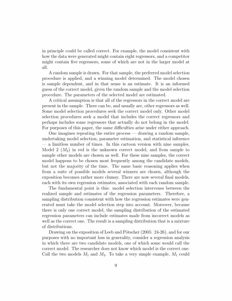
Figure 2 draws on equation 4. As before, there is a correct but unknownmodel. To simplify matters, and with no important loss of generality forthis demonstration, the mean squared errors for both regression models areassumed to be approximately 1.0. Then, the sampling distribution for β1,conditional on M1 being selected, is taken to be normal with a mean of 12.0and a standard deviation of 2.0. The sampling distribution for β1, condi-tional on M2 being selected, is taken to be normal with a mean of 4.0 and astandard deviation of 1. To minimize the complications, an ancilliary selec-tion procedure is applied such that P (M1) = .2 and P (M2) = .8; the modelselection procedure chooses M2 four times more often than M1. Figure 2 isconstructed by making 10,000 draws from the first normal distribution and40,000 draws from the second normal distribution. The line overlaid is thetrue combined distribution, which the simulation is meant to approximate.The combined distribution has a mean of approximately 5.6 and a standarddeviation of approximately 3.4.

The two sampling distributions, conditional on M1 or M2, are by designnormal, but the simulated sampling distribution after model selection is de-

11

Regression Coefficient Values

Density

0 5 10 15 20

0.00

0.05

0.10

0.15

0.20

0.25

0.30

Figure 2: An Illustrative Combined Sampling Distribution

12

cidedly non-normal. The distribution is bimodal and skewed to the right.Moreover, if M1 is the correct model, β1 from the combined distribution isbiased downward from 12.0 to 5.6. If M2 is the correct model, β1 is biasedupward from 4.0 to 5.6. In either case, the estimate will be systematicallyin error. The standard deviation of the combined distribution is substan-tially larger than the standard deviations of its constituent distributions: 3.4compared to 2.0 or 1.0. Again, the error is systematic.

Biased estimates of both regression coefficients and their standard errorsare to be anticipated in post-model-selection mixture distributions. More-over, the biases are unaffected by sample size; larger samples cannot beexpected to reduce the biases. Before one even gets to confidence intervalsand statistical tests, the estimation process can be badly compromised.8

In summary, model selection is a procedure by which some models arechosen over others. But model selection is subject to uncertainty. Becauseregression parameter estimates depend on the model in which they are em-bedded, there is in post-model-selection estimates additional uncertainty notpresent when a model is specified in advance. The uncertainty translatesinto sampling distributions that are a mixture of distributions, whose prop-erties can differ dramatically from those required for convention statisticalinference.

3.3 Underlying Mechanisms

Although mixed sampling distributions are the core problem, the particularforms a mixed distribution can take determine its practical consequences.It is necessary, therefore, to look under the hood. We need to consider thefactors that shape the mixed sampling distributions that can result frommodel selection. The specific mechanisms underlying post-model-selectionstatistical inference has apparently not been addressed in past work.

First, model selection implies that some regression coefficients values arecensored. If sufficiently close to zero, they are treated as equal to zero, andtheir associated regressors are dropped from the model. Consequently, a post-selection sampling distribution can be truncated or contain gaps in regionsthat are near 0.0. These effects are a direct result of the model selection.For example, Figure 2, might have censored at values β1 less than 2.0. There

8Simulations much like those in Section 4 can be used to produce virtually identicalresults starting with appropriate raw data and equations 2 and 3.

13

would have been no simulated values below that threshold.9

Second, there can be indirect effects. When for a given model a regressoris excluded, the performance of other regressors can be affected. For easeof exposition, as before suppose there are only two regressors, X and Z, ascandidate explanatory variables. Then, the sample regression coefficient forX holding Z constant can be written as,

βyx·z =ryx − rxzryz

(1− r2xz)

× sy

sx

, (5)

where r is a sample correlation coefficient, s is a sample standard deviation,and for both, the subscripts denote the regressors involved. Equation 5 isthe sample analogue of equation 1. If Z is dropped from the equation, all ofthe correlations involving Z are equivalent to 0.0. One is then left with thebivariate correlation between Y and X and the ratio of their two standarddeviations. Insofar as ryz and rxz are large in absolute value, the value of bxy·zcan change dramatically when Z is dropped from the model. Conversely, ifthe regressors are orthogonal (here, rxz = 0), regression coefficient estimateswill not be model dependent, and their sampling distributions will be unaf-fected by these indirect processes. These results generalize to models withmore than two candidate regressors.10

Third, sampling distributions can vary in their dispersion alone, althoughthis will typically be far less important than the direct or indirect effects ofmodel selection. One can see how the dispersion can be affected throughan equation for the standard error of a conventional regression coefficientestimate, not subject to model selection, say, βyx·z. For the two regressors Xand Z,

SE(βyx·z) =σε

sx

√n− 1

√1

1− r2xz

(6)

where σε is an estimate of the residual standard deviation, sx is the sam-ple standard deviation of x, and r2

xz is the square of the sample correlationbetween x and z.11 From this equation, one learns that the sampling distri-bution will be more dispersed if there is more residual variance, less variance

9The selection mechanism would then not have been ancillary.10The correlations in the numerator are replaced by partial correlations controlling for

all other predictors, and the correlation in the denominator is replaced by the multiplecorrelation of the predictor in question with all other predictors.

11Because in regression x and z are usually treated as fixed, sx and r2xz are not randomvariables and not treated as estimates.

14

in regressor x, more linear dependence between regressors, and a smaller sam-ple size. All except the sample size can be affected by the particular modelselected. In addition, σε is affected directly by random sampling error.12

The three underlying selection mechanisms — direct censoring, indirectcensoring, alterations in the dispersions of regression parameter estimates —can interact in complex ways that depend on the models considered and thedata being analyzed. There are, therefore, no general expressions throughwhich the impact of model selection may be summarized. However, simula-tions can provide some insight into what can happen. Because in simulationsone knows the model responsible for the data, there is a benchmark to whichthe post-model-selection results can be compared. When working with realdata, there is no known standard of absolute truth to which the empiricalresults can be held.13

4 Simulations of Model-Selection

We now turn to simulations of model selection effects. The form the selectiontakes is not a primary concern because in broad brush strokes at least, theimplications are the same regardless of how the selection is accomplished.For an initial simulation, selection is implemented through forward stepwiseregression using the AIC as a fit criterion. At each step, the term is addedthat leads to the model with the smallest AIC. The procedure stops whenno remaining regressor improves the AIC.

For this simulation, the full regression model takes the form of

yi = β0 + β1wi + β2xi + β3zi + εi, (7)

where β0 = 3.0, β1 = 0.0, β2 = 1.0, and β3 = 2.0. Because the parameterβ1 = 0 in equation 7, many would refer to a submodel that excluded W asthe “correct” model. But equation 7 is also correct as long at β1 = 0 isallowed. Therefore, we will use the adjective “preferred” for the model withw excluded. The full model and the preferred model will generate the sameconditional expectations for the response. The smaller model is preferredbecause it is simpler and uses up one less degree of freedom.

12When there are more than two regressors, the only change in equation 6 is that r2xz isreplaced by the square of the multiple correlation coefficient between the given regressorand all other regressors.

13If there were, there would be no need to do the research.

15

All three predictors are drawn at random from a multivariate normaldistribution, although with fixed regressors, this is of no importance. Thevariances and covariance are set as follows: σ2

ε = 10.0, σ2w = 5.0, σ2

x = 6.0,σ2

z = 7.0, σw,x = 4.0, σw,z = 5.0, and σx,z = 5.0. The sample size is 200. Theintent is to construct a data set broadly like data sets used in practice. Thedata were not constructed to illustrate a best case or worst case scenario.

10,000 samples were drawn, stepwise regression applied to each, and sam-pling distributions were constructed from the final models selected. Ratherthan plotting estimated regression coefficients, conventional t-values are plot-ted. The usual null hypothesis was assumed; each regression coefficient hasa population value 0.0. A distribution of t-values is more informative thana distribution of regression coefficients because it takes the regression co-efficients and their standard errors into account. The R2s varied over thesimulations between about .3 and .4.

4.1 Simulation Results

With three regressors, there are eight possible models, including a model inwhich none of the regressors is chosen. The distribution shown in Table 1indicates that the preferred model (i.e., with regressors X and Z) is selectedabout 66% of the time. The next most common model, chosen about 17% ofthe time, includes only regressor Z. The full model with regressors W , X,and Z is chosen 11% of the time. In short, for this simulation a practitionerhas a little less than a two-thirds chance of selecting the preferred model.

None W X Z WX WZ XZ WXZ0% 0% .0001% 17.4% 1.0% 4.9% 65.7% 10.8%

Table 1: Distribution of Models Selected in 10,000 Draws

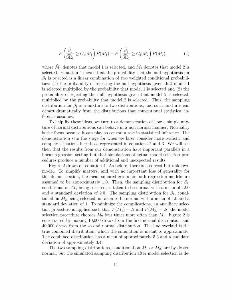
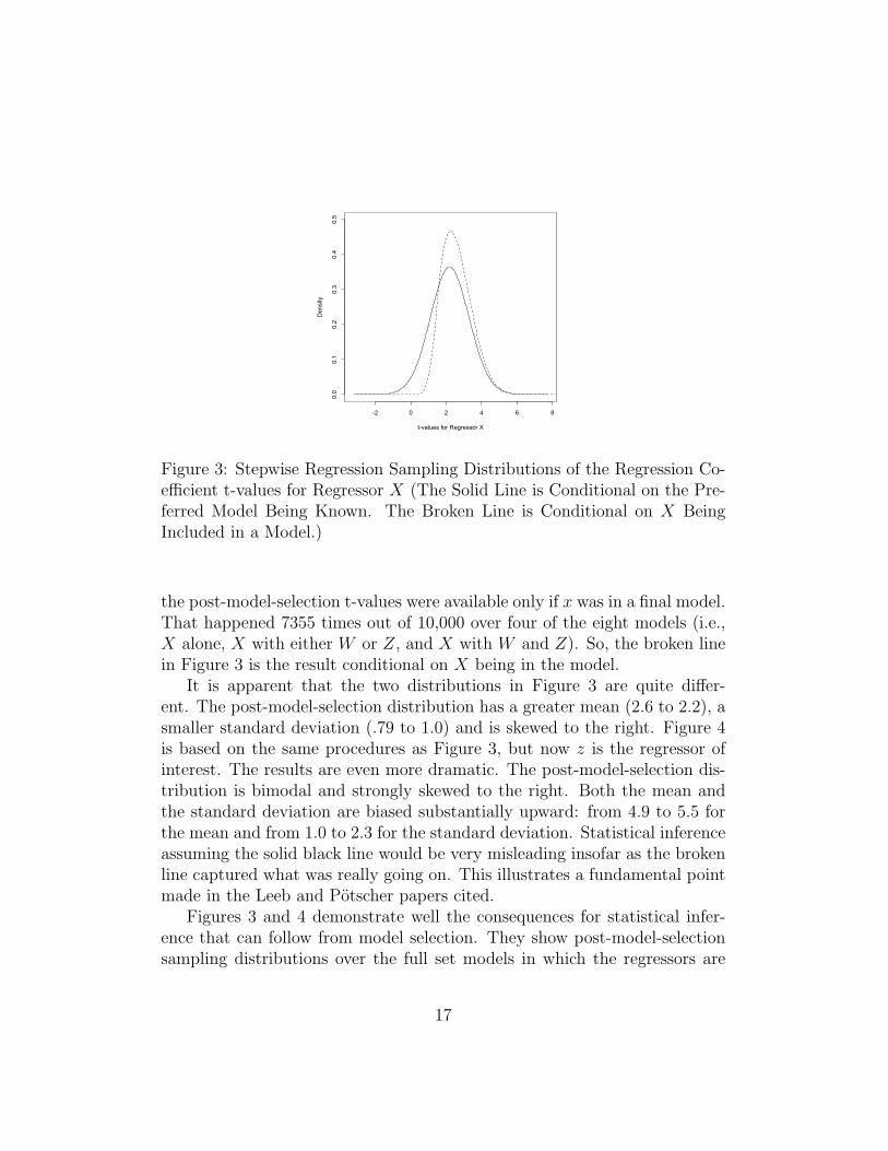
Figure 3 shows two simulated t-value distributions for regressor X. Thesolid black line represents the distribution that would result if the perferredmodel were known and its parameter values estimated; there is no modelselection. The broken line represents the post-model-selection sampling dis-tribution. Both lines are the product of a kernel density smoother appliedto the histograms from the simulation. The distribution assuming that thepreferred model was known was constructed from all the 10,000 samples. For

16

-2 0 2 4 6 8

0.0

0.1

0.2

0.3

0.4

0.5

t-values for Regressor X

Density

Figure 3: Stepwise Regression Sampling Distributions of the Regression Co-efficient t-values for Regressor X (The Solid Line is Conditional on the Pre-ferred Model Being Known. The Broken Line is Conditional on X BeingIncluded in a Model.)

the post-model-selection t-values were available only if x was in a final model.That happened 7355 times out of 10,000 over four of the eight models (i.e.,X alone, X with either W or Z, and X with W and Z). So, the broken linein Figure 3 is the result conditional on X being in the model.

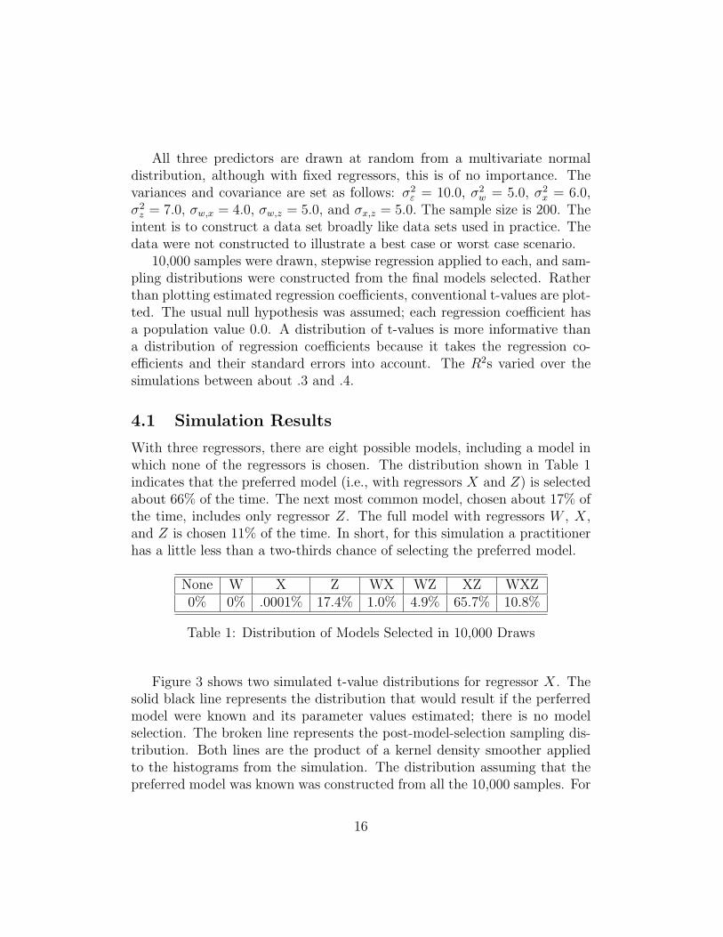
It is apparent that the two distributions in Figure 3 are quite differ-ent. The post-model-selection distribution has a greater mean (2.6 to 2.2), asmaller standard deviation (.79 to 1.0) and is skewed to the right. Figure 4is based on the same procedures as Figure 3, but now z is the regressor ofinterest. The results are even more dramatic. The post-model-selection dis-tribution is bimodal and strongly skewed to the right. Both the mean andthe standard deviation are biased substantially upward: from 4.9 to 5.5 forthe mean and from 1.0 to 2.3 for the standard deviation. Statistical inferenceassuming the solid black line would be very misleading insofar as the brokenline captured what was really going on. This illustrates a fundamental pointmade in the Leeb and Potscher papers cited.

Figures 3 and 4 demonstrate well the consequences for statistical infer-ence that can follow from model selection. They show post-model-selectionsampling distributions over the full set models in which the regressors are

17

0 2 4 6 8 10 12

0.0

0.1

0.2

0.3

0.4

0.5

t-values for Regressor Z

Density

Figure 4: Stepwise Regression Sampling Distributions of the Regression Co-efficient t-values for Regressor Z (The Solid Line is Conditional on the Pre-ferred Model Being Known. The Broken Line is Conditional on Z BeingIncluded in a Model.)

included. However, in practice researchers commonly settle on a final model,or a small number of final model candidates. Therefore, it is instructive toconsider the distributions of t-values conditional on a given model; a modelis chosen and tests are applied to that model only.

It is especially telling to condition on the preferred model even though inpractice the preferred model would not be known a priori. One might hopethat at least when the preferred model is selected, conventional statisticalinference would be on sound footing. However, selecting the preferred modelonly guarantees that the proper regressors are included. It does not guaranteeany of the desirable properties of the regression coefficient estimates.

Figures 5 shows that statistical inference remains problematic even whenthe statistical inference is conditional on arriving at the preferred model. Infact, Figure 5 and Figure 3 are very similar because for this simulation, xis usually selected as part of the chosen model. In effect, therefore, con-ditioning on the preferred model is already taking place much of the time.However, this is not a general result and is peripheral to our discussion inany case. The point is that the biases noted for Figures 3 remain. Thus,for the preferred model the null hypothesis that β2 = 0 should be rejected

18

-2 0 2 4 6 8

0.0

0.1

0.2

0.3

0.4

0.5

t-values for Regressor X

Density

Figure 5: Stepwise Regression Sampling Distributions of the Regression Co-efficient t-values for Regressor X. (The Solid Line is Conditional on thePreferred Model Being Known. The Broken Line is Conditional on the Pre-ferred Model Being Selected.)

at the .05 level with a probability of approximately .60. But after modelselection, that probability is about .76. This represents an increase of about27% driven substantially by bias in the estimated regression coefficient. Itis not a legitimate increase in power. False power seems to be a commonoccurrence for post-model-selection sampling distributions.

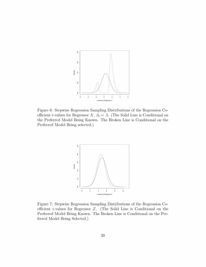
Figure 6 is constructed from the same simulation as Figure 5 except thatthe true value for β2 is now .5 not 1.0. The post-selection t-distribution,even when conditioning on the preferred model, is now strongly bimodaland nothing like the assumed normal distribution. The general point is thatthe post-model-selection sampling distribution can take on a wide variety ofshapes, none much like the normal, even when the researcher happens to haveselected the model accurately representing how the data were generated.

Figure 7 shows two distributions for Z, one based on the preferred modelbeing known (i.e., the solid line) and one conditioning on the selected pre-ferred model (i.e., the broken line). Figure 7 is very different from Figure 4.In this instance, conditioning on the selected preferred model brings theproper and post-model-selection distributions of t-values into a rough cor-respondence, and for both, the probability of rejecting at the .05 level the

19

-6 -4 -2 0 2 4 6

0.0

0.2

0.4

0.6

0.8

t-values for Regressor X

Density

Figure 6: Stepwise Regression Sampling Distributions of the Regression Co-efficient t-values for Regressor X, β2 = .5. (The Solid Line is Conditional onthe Preferred Model Being Known. The Broken Line is Conditional on thePreferred Model Being selected.)

0 2 4 6 8 10

0.0

0.1

0.2

0.3

0.4

0.5

t-values for Regressor Z

Density

Figure 7: Stepwise Regression Sampling Distributions of the Regression Co-efficient t-values for Regressor Z. (The Solid Line is Conditional on thePreferred Model Being Known. The Broken Line is Conditional on the Pre-ferred Model Being Selected.)

20

-2 0 2 4 6

0.0

0.1

0.2

0.3

0.4

0.5

t-values for Regressor X

Density

Figure 8: All Subsets Regression Sampling Distributions of the RegressionCoefficient t-values for Regressor X. (The Solid Line is Conditional on thePreferred Model Being Known. The Broken Line is Conditional on the Pre-ferred Model Being Selected.)

null hypothesis that β3 = 0 is about .99. This underscores that post-model-selection sampling distributions are not automatically misleading. Sometimesthe correct sampling distribution and the post-model-selection sampling dis-tribution will be very similar.

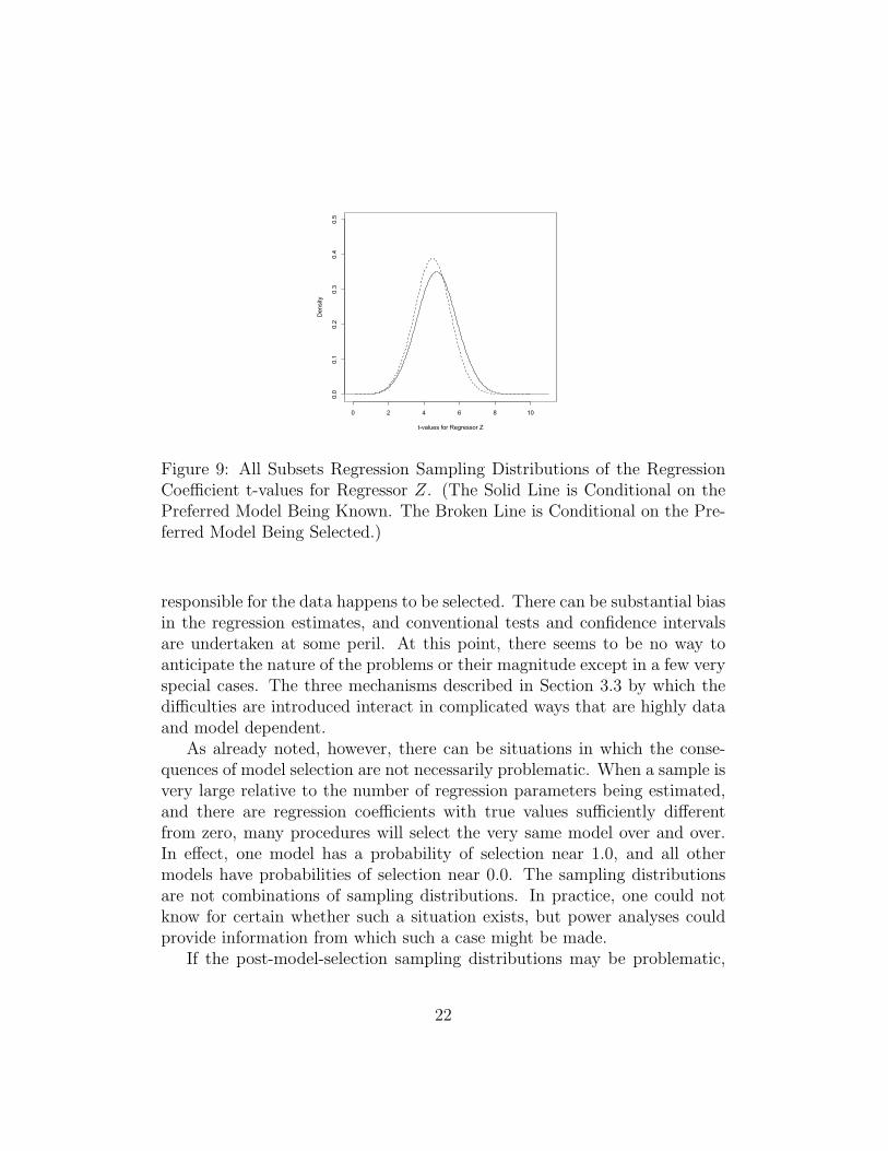
Figures 8 and 9 are a recapitulation but when selection is by all subsetsregression using Mallow’s Cp as the selection criterion. Much like the earlierstepwise regression, the correct model is chosen 64% of the time. Comparedto Figures 5 and 7, very little changes. As noted earlier, for purposes of thispaper the particular selection procedure used does not materially matter.The kinds of distortions introduced can vary with the selection procedure,but the overall message is unchanged. In this case, the distortions wereabout the same whether selection was by stepwise regression or all subsetsregression.

5 Potential Solutions

Post-model-selection sampling distributions can be highly non-normal, verycomplex, and with unknown finite sample properties even when the model

21

0 2 4 6 8 10

0.0

0.1

0.2

0.3

0.4

0.5

t-values for Regressor Z

Density

Figure 9: All Subsets Regression Sampling Distributions of the RegressionCoefficient t-values for Regressor Z. (The Solid Line is Conditional on thePreferred Model Being Known. The Broken Line is Conditional on the Pre-ferred Model Being Selected.)

responsible for the data happens to be selected. There can be substantial biasin the regression estimates, and conventional tests and confidence intervalsare undertaken at some peril. At this point, there seems to be no way toanticipate the nature of the problems or their magnitude except in a few veryspecial cases. The three mechanisms described in Section 3.3 by which thedifficulties are introduced interact in complicated ways that are highly dataand model dependent.

As already noted, however, there can be situations in which the conse-quences of model selection are not necessarily problematic. When a sample isvery large relative to the number of regression parameters being estimated,and there are regression coefficients with true values sufficiently differentfrom zero, many procedures will select the very same model over and over.In effect, one model has a probability of selection near 1.0, and all othermodels have probabilities of selection near 0.0. The sampling distributionsare not combinations of sampling distributions. In practice, one could notknow for certain whether such a situation exists, but power analyses couldprovide information from which such a case might be made.

If the post-model-selection sampling distributions may be problematic,

22

probably the most effective solution is to have two random samples from thepopulation of interest: a training sample and a test sample. The trainingsample is used to arrive at a preferred model. The test sample is used to es-timate the parameters of the chosen model and to apply statistical inference.For the test sample, the model is known in advance. The requisite struc-ture for proper statistical inference is in place, and problems resulting frompost-model-selection statistical inference are prevented. The dual-sample ap-proach is easy to implement once there are two samples.

When there is one sample, an option is to randomly partition that sampleinto two subsets. We call this the split-sample approach. One can then pro-ceed as if there were two samples to begin with. Whether this will work inpractice depends on the size each sample needs to be. Sample size determi-nations can be addressed by appropriate power analyses for each partition.

For example, suppose a researcher is prepared to assume, as required,that all of the necessary regressors in their appropriate functional forms areincluded in the data.14 The researcher also assumes that the regression coef-ficients associated with at least some of the regressors are actually 0.0. Thisis known as the assumption of “sparsity.” Then, the researcher assumes thatin the data the regressors belonging in the preferred model will have large re-gression coefficients relative to their standard errors and that regressors thatdo not belong in the preferred model will have small regression coefficientsrelative to their standard errors. It follows that a relatively small sample willbe able to find reliably the preferred model. The remaining data can serveas the test sample.

If the number of observations in the available data is too small to imple-ment a split-sample approach, one can fall back on a traditional textbookstrategy. Before the data are examined, a best guess is made about whatthe appropriate model should be. Parameter values can be estimated andstatistical inference applied just as the textbooks describe. If this confirma-tory step works out well, one can report the results with no concerns aboutpost-model-selection inference.15 One can then follow up with an exploratorydata analysis. A range of other models can be constructed and evaluated aslong as any statistical inference for selected models is not taken seriously.The exploratory results may well be very helpful for future research with

14This would include all necessary interaction effects.15All of the usual caveats would still apply. For example, if the model specified does not

properly represent how the data were generated, the regression estimates will be biased,and statistical tests will be not have their assumed properties.

23

new data. In short, there can be a confirmatory data analysis followed by anexploratory data analysis, each undertaken by its own inferential rules.

In the longer term, there are prospects for developing useful post-model-selection inference. A key will be to adjust properly for the additional uncer-tainty resulting from model selection. We are working on that problem andhave some initial promising results. Unfortunately, the implications may bedisappointing. It will probably turn out that when model uncertainty is prop-erly taken into account, confidence intervals will be far larger and statisticaltests will have substantially reduced power.

5.1 A Split-Sample Example

To help make the discussion of potential remedies more concrete, we turnbriefly to an empirical illustration using data on sentencing. Determinantsof post-conviction sentences have long been of interest to criminologists andto researchers from other disciplines who study sanctions (Blumstein et al.,1983; Wooldredge, 2005; Johnson, 2006). Probation decisions have receivedconsiderable attention (Morris and Tonry, 1980; Petersilia, 1997). When adecision is made to place an individual on probation, one might be interestedin the factors that could affect the length of the suspended incarceration sen-tence. Suspended sentence length can be important. It can be an ongoingthreat with which law-abiding behavior is shaped. It can also help to de-termine the length of the probation period and the probation conditionsimposed. Therefore, the factors that might help to explain the length ofsuspended sentences are important too.

We use real data and a split-sample approach. The data are a randomsample of 500 individuals sentenced to probation in a large American city.The length of the suspended sentence in months is the outcome of interest.For these data, mean sentence length is a little less than 28 months. Thedistribution is skewed to the right so that the median is only 18 months. 75%of the probationers have a suspended sentence of about 38 months or less.Because of the long right tail, it can make good sense to work with the log ofsentence length as the response variable. Using the log of sentence length isalso consistent with a theory that judges think in proportional terms whenthey determine sentence length. For instance, a sentence could be made 25%longer if an offender has a prior felony conviction.

The intent, therefore, is to consider how various features of the convictedindividual and the crimes for which the individual was convicted may be

24

related to log of sentence length.16 The follow regressors were available.

1. Assault as the conviction offense

2. Drug possession as the conviction offense

3. Burglary as the conviction offense

4. Gun-related crime as the conviction offense

5. Number of juvenile arrests

6. Number of prior arrests

7. Age at first contact with the adult courts

8. Age at conviction

9. Race black

10. Not married

11. High school degree

12. Referred for drug treatment

There were other conviction crimes in the data. But given the nature ofthis population, these crimes were never reported, or were reported so rarelythat they could not be used in the analysis. For example, if individualswere convicted of armed robbery, murder or rape, they were not placed onprobation. A substantial majority of the conviction offenses were for drug-related offenses, burglaries and assaults.

The regression model was not known before the data were analyzed. Con-sequently, the sample of 500 was partitioned at random into 250 trainingobservations and 250 test observations. All subsets regression was applied tothe training data with the BIC as the screening statistic.17 The parametersof the model selected were then estimated separately for the training and

16The logarithm of zero is undefined. So, a value of .5 (i.e., about two weeks) was usedinstead. Other reasonable strategies led to results that for purposes of this paper wereeffectively the same. A suspended sentence of zero months can occur, for instance, if asentencing judge gives sufficient credit for time served awaiting trial.

17The model selection was done with the procedure regsubsets in R.

25

the test data. Statistical tests were undertaken in both cases. The resultsfrom the test data do not suffer from the problems we have been consideringbecause the model was determined with another data set. But do the resultsfor the test data differ materially from the results for the training data? Wasthere a problem to be fixed?

There were three models that had very similar BIC values and very similarstructures. Table 2 shows the results for the model selected. Output fromthe other two models was much the same. The overall conclusions were aswell.

Four regressors were included: whether the conviction was for an assault,whether the conviction was for a drug offense, whether the conviction was fora gun-related offense, and the number of prior arrests. For each estimatedregression coefficient, we separately tested the null hypothesis that the pop-ulation regression coefficient was zero. A two-tailed tests was applied using.05 as the critical value.

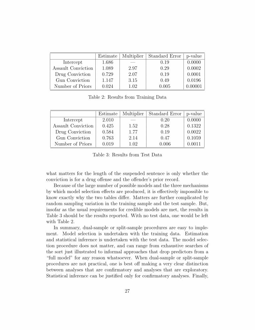
For the training data used to do the model selection, the null hypothesiswas easily rejected for each regressor, and the associations were all strong.Consistent with a theory that judges determine sentences proportionally, allof the regression coefficients were exponentiated so that they became multi-plicative constants. The baseline conviction offense is essentially burglary.18

Then in Table 2, the average burglary sentence is multiplied by 2.97 if theconviction offense is assault, by 2.07 if the conviction offense is for drugs,and by 3.15 if for a gun related offense. For each additional prior arrest, thesentence length is multiplied by 1.02. Thus, an offender with 10 prior ar-rests would have a sentence that is about 1.22 times longer than an offenderwith no prior arrests. In short, what matters is the conviction offense andprior record, with the multipliers that are substantial in practical terms. Fewcriminologists would find this surprising.

Table 3 shows the result when the same model is used with the test data.The results are rather different. Conviction for an assault or for a gun-relatedoffense are no longer statistically significant. Very small p-values in Table 2are greater the .05 in Table 3. The standard errors for the two regressioncoefficients are essentially unchanged, but the sizes of the regression coeffi-cients are substantially reduced. The other two regressors also show smallerassociations with the response in Table 3, but still have p-values less than.05. Thus, given the nature of the crimes for which one can receive probation,

18There is a scattering of a few other minor crimes are in the baseline.

26

Estimate Multiplier Standard Error p-valueIntercept 1.686 — 0.19 0.0000

Assault Conviction 1.089 2.97 0.29 0.0002Drug Conviction 0.729 2.07 0.19 0.0001Gun Conviction 1.147 3.15 0.49 0.0196

Number of Priors 0.024 1.02 0.005 0.00001

Table 2: Results from Training Data

Estimate Multiplier Standard Error p-valueIntercept 2.010 — 0.20 0.0000

Assault Conviction 0.425 1.52 0.28 0.1322Drug Conviction 0.584 1.77 0.19 0.0022Gun Conviction 0.763 2.14 0.47 0.1059

Number of Priors 0.019 1.02 0.006 0.0011

Table 3: Results from Test Data

what matters for the length of the suspended sentence is only whether theconviction is for a drug offense and the offender’s prior record.

Because of the large number of possible models and the three mechanismsby which model selection effects are produced, it is effectively impossible toknow exactly why the two tables differ. Matters are further complicated byrandom sampling variation in the training sample and the test sample. But,insofar as the usual requirements for credible models are met, the results inTable 3 should be the results reported. With no test data, one would be leftwith Table 2.

In summary, dual-sample or split-sample procedures are easy to imple-ment. Model selection is undertaken with the training data. Estimationand statistical inference is undertaken with the test data. The model selec-tion procedure does not matter, and can range from exhaustive searches ofthe sort just illustrated to informal approaches that drop predictors from a“full model” for any reason whatsoever. When dual-sample or split-sampleprocedures are not practical, one is best off making a very clear distinctionbetween analyses that are confirmatory and analyses that are exploratory.Statistical inference can be justified only for confirmatory analyses. Finally,

27

model selection by itself implies little about the ultimate credibility of themodel chosen. Conventional assumption still have to be reasonable well met.

6 Conclusions

There is no doubt that post-model-selection statistical inference can leadto biased regression parameter estimates and seriously misleading statisticaltests and confidence intervals. The approaches by which the selection is doneare for the issues raised in this paper unimportant. Informal data snoopingis as dangerous as state-of-the-art model selection procedures.

Currently, there are five possible responses. If a case can be made foran appropriate model before the data are analyzed, one can proceed as thetextbooks describe. Alternatively, the problem can be ignored if one cancredibly argue that the model selection procedures will select a single modelwith a probability of near 1.0. If there are two random samples from thesame population, or if it is possible to construct the equivalent from the dataon hand, appropriate statistical inference may be undertaken even if thereare substantial post-model-selection difficulties. When neither approach ispractical, one can make a clear distinction between data analyses that areconfirmatory and analyses that are exploratory. Statistical inference is ap-propriate only for the former. Finally, should all else fail, one can simplyforego formal statistical inference altogether.

If after model selection, there remains more than one candidate model,new complications are introduced. The underlying inferential logic is flawed.If there are several candidate models, at best only one can correctly representhow the data were generated. The confidence intervals and statistical testsfor all models but one will not perform as required, and the one model forwhich statistical inference can be appropriate is unknown. There is also thereal possibility that all of the models are suspect in which case, all of the testsand confidence intervals can be compromised. In short, post-model-selectionstatistical inference can be further jeopardized when more than one model isselected.

28

References

Barnett, V. (1983) Comparative Statistical Inference, second edition. NewYork: John Wiley and Sons.

Benjamini, Y., and D. Yekutieli (2001) “The Control of the False Discov-ery Rate in Multiple Testing Under Dependency,” Annals of Statistics29(4): 1165–188.

Berk, R.A., (2003) Regression Analysis: A Constructive Critique, NewburyPark, CA, Sage Publications.

Blumstein, A., Cohen, J., Martin, S.E., and M.H. Tonrey (eds.) (1983)Research on Sentencing: The Search for Reform, Volumes 1 and 2.Washington, D.C.: National Academy Press.

Box, G.E.P. (1976) “Science and Statistics.” Journal of the American Sta-tistical Association 71: 791–799.

Breiman, L. (2001) “Statistical Modeling: Two Cultures” (with discussion).Statistical Science 16: 199–231.

Brown, L.D. (1967) “The Conditional Level of Student’s t Test,” The Annalsof Mathematical Statistics 38(4): 1068–1071.

Brown, L.D. (1990) “An Ancillarity Paradox which Appears in MultipleLinear Regression,” The Annals of Statistics 18(2): 471-493.

Candes, E., and T. Tao (2007) “The Dantzig Selector: Statistical Estimationwheb p is much larger than n,” The Annals of Statistics 35(6): 2313–2331.

Cook, D.R., and S. Weisberg (1999) Applied Regression Including Comput-ing and Graphics. New York: John Wiley and Sons.

Davies, G., and K. Dedel (2006) “Violence Screening in Community Cor-rections,” Criminology & Public Policy 5(4): 743–770.

Efron, B., Hastie, T. , and R. Tibshinani (2007) “Discussion: The DantzigSelector: Statistical Estimation with p Much Larger than n,” The An-nals of Statistics 35(6) 2358-2364.

29

Efron, B. (2007) “Correlation and Large-Scale Simultaneous SignificanceTesting,”Journal of the American Statistical Association 102(477) 93–103

Freedman, D.A. (1987) “As Others See Us: A Case Study in Path Analysis”(with discussion). Journal of Educational Statistics 12: 101–223.

Freedman, D.A. (2004) “Graphical Models for Causation and the Identifi-cation Problem.” Evaluation Review 28: 267–293.

Freedman, D.A. (2005) Statistical Models: Theory and Practice, Cambridge;Cambridge University Press.

Freedman, D.A., Navidi, W., and S.C. Peters (1988) “On the Impact of Vari-able Selection in Fitting Regression Equations.” In T.K. Dijkstra (ed.),On Model Uncertainty and Its Statistical Implications, 1–16, Springer,Berlin.

Greene, W.H. (2003) Econometric Methods, fifth edition, New Yortk: Pren-tice Hall.

Johnson, B.D., (2006) “The Multilevel Context of Criminal Sentencing:Integrating Judge- and County-Level Influences.” Criminology 44(2):235–258.

Lalonde, R.J., and R.M. Cho (2008) “The Impact of Incarceration in StatePrison on the Employment Prospects of Women,” Journal of Quanti-tative Criminology 24: 243–265.

Leeb, H., B.M. Potscher (2005) “Model Selection and Inference: Facts andFiction,” Econometric Theory 21: 21–59.

Leeb, H., B.M. Potscher (2006) “Can one Estimate the Conditional Distri-bution of Post-Model-Selection Estimators?” The Annals of Statistics34(5): 2554–2591.

Leeb, H., B.M. Potscher (2008) “Model Selection,” in T.G. Anderson, R.A.Davis, J.-P. Kreib, and T. Mikosch (eds.), The Handbook of FinancialTime Series, New York, Springer: 785–821.

Leamer, E.E. (1978) Specification Searches: Ad Hoc Inference with Non-Experimental Data. New York, John Wiley.

30

Manski, C.F. (1990) “Nonparametric Bounds on Treatment Effects.” Amer-ican Economic Review Papers and Proceedings 80: 319–323.

McCullagh, P. and J.A. Nelder (1989) Generalized Linear Models, secondedition, New York, Chapman & Hall.

Morgan, S.L. and C. Winship (2007) Counterfactuals and Causal Inference:Methods and Principles for Social Research, Cambridge: CambridgeUniversity Press.

Morris, N., and M. Tonry (1990) Prison and Probation: Intermediate Pun-ishment in a Rational Sentencing System. New York” Oxford Univer-sity Press.

Olshen, R. A., (1973) “The Conditional Level of the F-Test,” Journal of theAmerican Statistical Association 68(343): 692–698.

Ousey, G.C., Wilcox, P. and S. Brummel (2008) “Deja vu All Over Again:Investigating Temporal Continuity of Adolescent Victimization,” Jour-nal of Quantitative Criminology 24: 307–335.

Petersilia, J. (1997) “Probation in the United States.” Crime and Justice22: 149-200.

Rubin, D. B. (1986) “Which Ifs Have Causal Answers.” Journal of theAmerican Statistical Association 81: 961–962.

Sampson, R.J. and S.W. Raudenbush (2004) “Seeing Disorder: Neoghbor-hood Stigma and the Social Construction of “Broken Windows,” SocialPsychology Quarterly 67(4): 319-342.

Schroeder, R.D., Giordano, P.C., and S.A. Cernkovich (2007) “Drug useand Disistance Processes,” Criminology 45(1): 191–222.

Wooldredge, J., Griffin, T., and F. Rauschenberg (2005) “(Un)anticipatedEffects of Sentencing REform on Disparate Treatment of Defendants.”Law & Society Review 39(4) 835-874.

31