Graduate Theses, Dissertations, and Problem Reports 2020 Statistical Assessment of the Significance of Fracture Fits in Statistical Assessment of the Significance of Fracture Fits in Trace Evidence Trace Evidence Evie K. Brooks West Virginia University, [email protected] Follow this and additional works at: https://researchrepository.wvu.edu/etd Part of the Forensic Science and Technology Commons Recommended Citation Recommended Citation Brooks, Evie K., "Statistical Assessment of the Significance of Fracture Fits in Trace Evidence" (2020). Graduate Theses, Dissertations, and Problem Reports. 7704. https://researchrepository.wvu.edu/etd/7704 This Thesis is protected by copyright and/or related rights. It has been brought to you by the The Research Repository @ WVU with permission from the rights-holder(s). You are free to use this Thesis in any way that is permitted by the copyright and related rights legislation that applies to your use. For other uses you must obtain permission from the rights-holder(s) directly, unless additional rights are indicated by a Creative Commons license in the record and/ or on the work itself. This Thesis has been accepted for inclusion in WVU Graduate Theses, Dissertations, and Problem Reports collection by an authorized administrator of The Research Repository @ WVU. For more information, please contact [email protected].

Welcome message from author
This document is posted to help you gain knowledge. Please leave a comment to let me know what you think about it! Share it to your friends and learn new things together.
Transcript
Graduate Theses, Dissertations, and Problem Reports
2020
Statistical Assessment of the Significance of Fracture Fits in Statistical Assessment of the Significance of Fracture Fits in
Trace Evidence Trace Evidence
Evie K. Brooks West Virginia University, [email protected]
Follow this and additional works at: https://researchrepository.wvu.edu/etd
Part of the Forensic Science and Technology Commons
Recommended Citation Recommended Citation Brooks, Evie K., "Statistical Assessment of the Significance of Fracture Fits in Trace Evidence" (2020). Graduate Theses, Dissertations, and Problem Reports. 7704. https://researchrepository.wvu.edu/etd/7704
This Thesis is protected by copyright and/or related rights. It has been brought to you by the The Research Repository @ WVU with permission from the rights-holder(s). You are free to use this Thesis in any way that is permitted by the copyright and related rights legislation that applies to your use. For other uses you must obtain permission from the rights-holder(s) directly, unless additional rights are indicated by a Creative Commons license in the record and/ or on the work itself. This Thesis has been accepted for inclusion in WVU Graduate Theses, Dissertations, and Problem Reports collection by an authorized administrator of The Research Repository @ WVU. For more information, please contact [email protected].
Graduate Theses, Dissertations, and Problem Reports
2020
Statistical Assessment of the Significance of Fracture Fits in Statistical Assessment of the Significance of Fracture Fits in
Trace Evidence Trace Evidence
Evie K. Brooks
Follow this and additional works at: https://researchrepository.wvu.edu/etd
Part of the Forensic Science and Technology Commons
Statistical Assessment of the Significance of Fracture Fits in Trace Evidence
Evie K. Brooks
Thesis submitted
to the Eberly College of Arts and Sciences
at West Virginia University
in partial fulfillment of the requirements for the degree of
Master of Science in
Forensic and Investigative Science
Tatiana Trejos, Ph.D., Chair
Keith Morris, Ph.D.
Andria Mehltretter, M.S.
Department of Forensic and Investigative Science
Morgantown, West Virginia
2020
Keywords: trace evidence, physical fit, duct tape, inter-laboratory study, textiles, X-ray
fluorescence, electrical tape
Copyright 2020 Evie K. Brooks
ABSTRACT
Statistical Assessment of the Significance of Fracture Fits in Trace Evidence
Evie K. Brooks
Fracture fits are often regarded as the highest degree of association of trace materials due to the
common belief that inherently random fracturing events produce individualizing patterns. Often
referred to as physical matches, fracture matches, or physical fits, these assessments consist of the
realignment of two or more items with distinctive features and edge morphologies to demonstrate
they were once part of the same object. Separated materials may provide a valuable link between
items, individuals, or locations in forensic casework in a variety of criminal situations. Physical fit
examinations require the use of the examiner’s judgment, which rarely can be supported by a
quantifiable uncertainty or vastly reported error rates.
Therefore, there is a need to develop, validate, and standardize fracture fit examination
methodology and respective interpretation protocols. This research aimed to develop systematic
methods of examination and quantitative measures to assess the significance of trace evidence
physical fits. This was facilitated through four main objectives: 1) an in-depth review manuscript
consisting of 112 case reports, fractography studies, and quantitative-based studies to provide an
organized summary establishing the current physical fit research base, 2) a pilot inter-laboratory
study of a systematic, score-based technique previously developed by our research group for
evaluation of duct tape physical fit pairs and referred as the Edge Similarity Score (ESS), 3) the
initial expansion of ESS methodology into textile materials, and 4) an expanded optimization and
evaluation study of X-ray Fluorescence (XRF) Spectroscopy for electrical tape backing analysis,
for implementation in an amorphous material of which physical fits may not be feasible due to
lack of distinctive features.
Objective 1 was completed through a large-scale literature review and manuscript compilation of
112 fracture fit reports and research studies. Literature was evaluated in three overall categories:
case reports, fractography or qualitative-based studies, and quantitative-based studies. In addition,
12 standard operating protocols (SOP) provided by various state and federal-level forensic
laboratories were reviewed to provide an assessment of current physical fit practice. A review
manuscript was submitted to Forensic Science International and has been accepted for publication.
This manuscript provides for the first time, a literature review of physical fits of trace materials
and served as the basis for this project.
The pilot inter-laboratory study (Objective 2) consisted of three study kits, each consisting of 7
duct tape comparison pairs with a ground truth of 4 matching pairs (3 of expected M+ qualifier
range, 1 of the more difficult M- range) and 3 non-matching pairs (NM). The kits were distributed
as a Round Robin study resulting in 16 overall participants and 112 physical fit comparisons. Prior
to kit distribution, a consensus on each sample’s ESS was reached between 4 examiners with an
agreement criterion of better than ± 10% ESS. Along with the physical comparison pairs, the study
included a brief, post-study survey allowing the distributors to receive feedback on the
participants’ opinions on method ease of use and practicality. No misclassifications were observed
across all study kits. The majority (86.6%) of reported ESS scores were within ± 20 ESS compared
to consensus values determined before the administration of the test. Accuracy ranged from 88%
to 100%, depending on the criteria used for evaluation of the error rates. In addition, on average,
77% of ESS attributed no significant differences from the respective pre-distribution, consensus
mean scores when subjected to ANOVA-Dunnett’s analysis using the level of difficulty as
blocking variables. These differences were more often observed on sets of higher difficulty (M-,
5 out of 16 participants, or 31%) than on lower difficulty sets (M+ or M-, 3 out of 16 participants,
or 19%). Three main observations were derived from the participant results: 1) overall good
agreement between ESS reported by examiners was observed, 2) the ESS score represented a good
indicator of the quality of the match and rendered low percent of error rates on conclusions 3)
those examiners that did not participate in formal method training tended to have ESS falling
outside of expected pre-distribution ranges. This interlaboratory study serves as an important
precedent, as it represents the largest inter-laboratory study ever reported using a quantitative
assessment of physical fits of duct tapes. In addition, the study provides valuable insights to move
forward with the standardization of protocols of examination and interpretation.
Objective 3 consisted of a preliminary study on the assessment of 274 total comparisons of stabbed
(N=100) and hand-torn (N=174) textile pairs as completed by two examiners. The first 74
comparisons resulted in a high incidence of false exclusions (63%) on textiles prone to distortion,
revealing the need to assess suitability prior to physical fit examination of fabrics. For the
remaining dataset, five clothing items were subject to fracture of various textile composition and
construction. The overall set consisted of 100 comparison pairs, 20 per textile item, 10 each per
separation method of stabbed or hand-torn fractured edges, each examined by two analysts.
Examiners determined ESS through the analysis of 10 bins of equal divisions of the total fracture
edge length. A weighted ESS was also determined with the addition of three optional weighting
factors per bin due to the continuation of a pattern, separation characteristics (i.e. damage or
protrusions/gaps), or partial pattern fluorescence across the fractured edges. With the addition of
a weighted ESS, a rarity ratio was determined as the ratio between the weighted ESS and non-
weighted ESS. In addition, the frequency of occurrence of all noted distinctive characteristics
leading to the addition of a weighting factor by the examiner was determined. Overall, 93%
accuracy was observed for the hand-torn set while 95% accuracy was observed for the stabbed set.
Higher misclassification in the hand-torn set was observed in textile items of either 100% polyester
composition or jersey knit construction, as higher elasticity led to greater fracture edge distortion.
In addition, higher misclassification was observed in the stabbed set for those textiles of no pattern
as the stabbed edges led to straight, featureless bins often only associated due to pattern
continuation. The results of this study are anticipated to provide valuable knowledge for the future
development of protocols for evaluation of relevant features of textile fractures and assessments
of the suitability for fracture fit comparisons.
Finally, the XRF methodology optimization and evaluation study (Objective 4) expanded upon
our group’s previous discrimination studies by broadening the total sample set of characterized

tapes and evaluating the use of spectral overlay, spectral contrast angle, and Quadratic
Discriminant Analysis (QDA) for the comparison of XRF spectra. The expanded sample set
consisted of 114 samples, 94 from different sources, and 20 from the same roll. Twenty sections
from the same roll were used to assess intra-roll variability, and for each sample, replicate
measurements on different locations of the tape were analyzed (n=3) to assess the intra-sample
variability. Inter-source variability was evaluated through 94 rolls of tapes of a variety of labeled
brands, manufacturers, and product names. Parameter optimization included a comparison of
atmospheric conditions, collection times, and instrumental filters. A study of the effects of
adhesive and backing thickness on spectrum collection revealed key implications to the method
that required modification to the sample support material Figures of merit assessed included
accuracy and discrimination over time, precision, sensitivity, and selectivity. One of the most
important contributions of this study is the proposal of alternative objective methods of spectral
comparisons. The performance of different methods for comparing and contrasting spectra was
evaluated. The optimization of this method was part of an assessment to incorporate XRF to a
forensic laboratory protocol for rapid, highly informative elemental analysis of electrical tape
backings and to expand examiners’ casework capabilities in the circumstance that a physical fit
conclusion is limited due to the amorphous nature of electrical tape backings.
Overall, this work strengthens the fracture fit research base by further developing quantitative
methodologies for duct tape and textile materials and initiating widespread distribution of the
technique through an inter-laboratory study to begin steps towards laboratory implementation.
Additional projects established the current state of forensic physical fit to provide the foundation
from which future quantitative work such as the studies presented here must grow and provided
highly sensitive techniques of analysis for materials that present limited fracture fit capabilities.

v
ACKNOWLEDGEMENTS
I would first like to express my appreciation to my research advisor and committee chair, Dr.
Tatiana Trejos. Over the past two years the guidance, time, and commitment she has put into
assisting me in my research endeavors has shaped who I am as a student, as well as the project into
what it is today. I am very grateful for the support and encouragement she provided me, as well as
for the academic and professional lessons she has taught me through the years.
I would also like to thank my committee members, Dr. Keith Morris and Andria Mehltretter for
the support and assistance they provided throughout the project. Your insight was always
appreciated and greatly furthered the progression and growth of my ideas.
In addition, I would like to specifically thank Andria for the guidance and dedication she has shown
during my graduate career as well as my time as her intern. The personal and professional growth
you inspired as a supervisor has broadened my path and strengthened my commitment to the field.
I am thankful to my fellow research group members for their comradery and support throughout
our time together. I would also like to thank my departmental peers for the friendships that have
lifted me up and helped me to navigate my time at West Virginia University.
Finally, I would like to express my gratitude to my incredible support system: my parents Jeff and
Lisa, my sister Katie, my brother Grayson, and my fiancé Brandon. Thank you for the endless
encouragement and unconditional love you have always shown that was only greater magnified
by this experience. Everything I am I owe to you.
vi
TABLE OF CONTENTS
Abstract .......................................................................................................................................... ii
Acknowledgements ........................................................................................................................v
Table of Contents ......................................................................................................................... vi
Table of Figures.......................................................................................................................... viii
List of Tables .............................................................................................................................. xiii
I. Overall Introduction ..................................................................................................................1
II. Chapter 1. Forensic Physical Fits in the Trace Evidence Discipline: A Review .................5
1.1. Abstract ..................................................................................................................................5
1.2. Introduction ............................................................................................................................5
1.3. Physical Fits in Trace Evidence – Current Protocol Examples .............................................9
1.4. Established Physical Fit Research .......................................................................................12
1.5. Strengths and Limitations ....................................................................................................39
1.6. Conclusions ..........................................................................................................................40
1.7. Acknowledgements ..............................................................................................................41
1.8. References ............................................................................................................................42
1.9. Supplementary Material .......................................................................................................49
III. Chapter 2. Inter-Laboratory Assessment of the Utility of the Edge Similarity Score (ESS)
in Duct Tape Physical Fit Examinations ....................................................................................85
2.1. Overview of the Inter-Laboratory Study .............................................................................85
2.2. Introduction .........................................................................................................................87
2.3. Materials and Methods ........................................................................................................89
2.4. Results and Discussion ........................................................................................................97
2.5. Conclusions and Future Work ...........................................................................................136
2.6. References .........................................................................................................................138
2.7. Appendix A .......................................................................................................................140
2.8. Appendix B .......................................................................................................................153
IV. Chapter 3. Steps Toward Quantitative Assessment of Textile Physical Fits – Expansion
of the Edge Similarity Score (ESS) Method ............................................................................158
3.1. Overview of the Textile Fracture Study ............................................................................158
vii
3.2. Introduction .......................................................................................................................159
3.3. Materials and Methods ......................................................................................................162
3.4. Results and Discussion ......................................................................................................173
3.5. Conclusions and Future Work ...........................................................................................191
3.6. References .........................................................................................................................192
V. Chapter 4. Optimization and Evaluation of Spectral Comparisons of Electrical Tape
Backings by X-ray Fluorescence ..............................................................................................194
4.1. Abstract .............................................................................................................................194
4.2. Introduction .......................................................................................................................194
4.3. Methods .............................................................................................................................198
4.4. Results ...............................................................................................................................205
4.5. Conclusions .......................................................................................................................221
4.6. Acknowledgements ...........................................................................................................221
4.7. References .........................................................................................................................222
4.8. Supplementary Material ....................................................................................................224
4.9. Appendix ...........................................................................................................................225
VI. Overall Conclusions and Future Work .............................................................................230
VII. Overall References (Introduction and Conclusions/Future Work Sections) ...............234
viii
TABLE OF FIGURES
Chapter 1
Figure 1. Reviewed physical fit literature by category and material type (n=79 publications;
articles discussing more than one material type are duplicated in the count of each relevant
category)
Chapter 2
Figure 1. Comparison edge morphology classification for two examples of matching pairs (A and
C) and one example of a non-matching pair (B)
Figure 2. Inter-laboratory modified petal test distribution
Figure 3. Backing physical feature examples: A) dimpling, B) calendering striae, C) backing
distortion
Figure 4. Adhesive and scrim physical feature examples: A) warp scrim alignment/continuation
of scrim pattern, B) protruding warp yarns, C) adhesive distortion, D) double weft edge scrim, E)
missing scrim
Figure 5. Pre-distribution, consensus ESS values per sample per kit (N=4 examiners)
Figure 6. Kit 1 examiner ESS variation as compared to pre-distribution mean (consensus: N=4
examiners)
Figure 7. Kit 2 examiner ESS variation as compared to pre-distribution mean (consensus: N=4
examiners)
Figure 8. Kit 3 examiner ESS variation as compared to pre-distribution mean (consensus: N=4
examiners)
Figure 9. Kit 1 examiner ESS variation as compared to consensus mean ± 20% threshold
Figure 10. Kit 2 examiner ESS variation as compared to consensus mean ± 20% threshold
Figure 11. Kit 3 examiner ESS variation as compared to consensus mean ± 20% threshold
Figure 12. Kit 1 examiner ESS variation as compared to expected comparison edge qualifier
thresholds
Figure 13. Kit 2 examiner ESS variation as compared to expected comparison edge qualifier
thresholds
Figure 14. Kit 3 examiner ESS variation as compared to expected comparison edge qualifier
thresholds
Figure 15. Boxplot ESS distributions of inter-laboratory sample pairs grouped as M+, M-, and
NM
Figure 16. Dunnett’s test examiner control differences results, M+, M-, and NM samples
ix
Figure 17. Kit 1 ESS distribution by overall conclusion (N=6 examiners, n=42 total comparisons).
Numbering indicates discrepancy instances, points of discussion in which results varied from those
expected.
Figure 18. Kit 1 samples, treatment of “featureless” scrim bins, red areas indicate bins marked “0”
by participant
Figure 19. Kit 1 samples, treatment of distorted scrim bins, red areas indicate bins marked “0” by
participant
Figure 20. Kit 2 ESS distribution by overall conclusion (N=3 examiners, n=21 total comparisons)
Figure 21. Kit 3 ESS distribution by overall conclusion (N=7 examiners, n=49 total comparisons).
Numbering indicates discrepancy instances, points of discussion in which results varied from those
expected.
Figure 22. Kit 3 sample, treatment of “featureless” scrim bins, green areas indicate bins marked
“1” by participant
Figure 23. Kit 3 sample, treatment of distorted scrim bins, green areas indicate bins marked “1”
by participant
Figure 24. Kit 1 ESS distribution by qualifier (N=6 examiners, n=42 total comparisons).
Numbering indicates discrepancy instances, points of discussion in which results varied from those
expected.
Figure 25. Kit 1 samples, qualifiers out of expected ranges, red areas indicate bins marked “0” by
participant
Figure 26. Kit 2 ESS distribution by qualifier (N=3 examiners, n=21 total comparisons).
Numbering indicates discrepancy instances, points of discussion in which results varied from those
expected.
Figure 27. Kit 2 samples, qualifiers out of expected ranges, red areas indicate bins marked “0” by
participant while green areas indicate bins marked “1”
Figure 28. Comparison of Kit 2 samples assigned same ESS but different comparison edge
qualifiers by same participant, red areas indicate bins marked “0” by participant
Figure 29. Kit 3 ESS distribution by qualifier (N=7 examiners, 49 total comparisons). Numbering
indicates discrepancy instances, points of discussion in which results varied from those expected.
Figure 30. Comparison of Kit 3 samples assigned same ESS but different comparison edge
qualifiers by same participant, green areas indicate bins marked “1” by participant
Figure 31. Comparison of Kit 3 samples assigned same ESS but different comparison edge
qualifiers by same participant, red areas indicate bins marked “0” by participant
Figure 32. Kit 3 samples, qualifiers out of expected ranges, red areas indicate bins marked “0” by
participant while green areas indicate bins marked “1”
x
Figure 33. Overall inter-laboratory study ESS distribution
Figure 34. Prusinowski et al.1 medium quality, hand torn duct tape physical fit dataset (N=508
comparison pairs per analyst)
Chapter 2: Appendix B
Figure i. Survey question 1 results
Figure ii. Survey question 2 results
Figure iii. Survey question 3 results
Figure iv. Survey question 4 results
Figure v. Survey question 5 results
Figure vi. Survey question 6 results
Figure vii. Survey question 7 results
Figure viii. Survey question 8 results
Figure ix. Survey question 9 results
Chapter 3
Figure 1. Foam human form fracturing substrate
Figure 2. Textile sample set experimental design schematic
Figure 3. General characteristic example – color
Figure 4. General characteristic example – fabric construction (twill weave)
Figure 5. General characteristic example – general fiber size/shape
Figure 6. General characteristic example – fiber twist (“Z” twist)
Figure 7. General characteristic example – alignment of long short threads. Note: Region
highlighted indicates an area considered a distinctive characteristic (i.e. gap/protrusion)
Figure 8. General characteristic example – general fluorescence (Note: The dark square regions
on the right and left image are sample labels, not a region within the fabric’s pattern.)
Figure 9. Distinctive characteristic example – pattern continuation across fracture
Figure 10. Distinctive characteristic example – separation characteristics (e.g. fabric damage
continuation across fracture – a “gather” or pulled thread within the fabric weave)
Figure 11. Distinctive characteristic example – separation characteristics (e.g. protrusions/gaps
consistent across fracture)
Figure 12. Distinctive characteristic example – partial pattern fluorescence
xi
Figure 13. Edge curling in preliminary set fabric
Figure 14. Overall conclusion and comparison edge qualifier comparison between two examiners,
preliminary Set A (100% hand-torn, jersey knit polyester)
Figure 15. Preliminary textile set false negative examples
Figure 16. Item A edge morphology true match examples – a) hand-torn edges, b) stabbed edges
Figure 17. Examiner B false positive – Item D
Figure 18. Examiner B false negative – Item D
Figure 19. Examiner B false negative – Item E
Figure 20. Examiner B inconclusive (true match sample) – Item E
Figure 21. Examiner B inconclusive (true match sample) – Item D
Figure 22. Examiner B false negative – Item D
Figure 23. Examiner B inconclusive (true non-match sample) – Item A
Figure 24. Examiner B inconclusive (true match sample) – Item B
Figure 25. Examiner A inconclusive (true match sample) – Item B
Figure 26. Hand-torn sample set ESS distribution boxplots
Figure 27. Stabbed sample set ESS distribution boxplots
Figure 28. Rarity ratio distribution – hand-torn sample set
Figure 29. Rarity ratio distribution – stabbed sample set
Figure 30. Graphical display of relative frequency of occurrence of weighting factor assignment
(Note: fluorescence observations for Item B are being revisited in future work)
Chapter 4
Figure 1. Spectra overlay comparison of tape 45 run both in air (3 reps) and under vacuum (3
reps), low Zc filter
Figure 2. Spectra overlay of Be and lucite planchets, low Zc filter
Figure 3. Spectra overlay comparison of tape 33 run both with adhesive (3 reps) and without
adhesive (3 reps), low Zc filter
Figure 4. Spectra overlay of stretched and pristine sample 12 run with the Be planchet, low Zc
filter
Figure 5. Ca/Sb low Zc interference and high Zb resolved Sb, sample 91
xii
Figure 6. Comparison of ranges of contrast angle ratios variation for intra-samples
(indistinguishable subgroup samples, same roll samples), and inter-samples (between groups and
between subgroup samples). The inset shows a zoomed area of the plot.
Figure 7. QDA canonical plot by manufacturing origin for optimized filter overall tape data set
(N=94)
Figure 8. Spectral contrast angle intra-roll sample variation as compared to inter-group variation.
8a: Box plots of intra-roll (low Zc and high Zb and inter-group. 8b: Display of spectral contrast
angle ratio for 190 comparison pairs of tape samples from the same roll.
Chapter 4: Appendix
Figure A.1. Inter-group SNR differences in present vs. absent elements: sample 65 (Pb present
with SNR=301.28) and sample 75 (Pb absent with SNR=0.74), mid Zc filter
Figure A.2. Inter-subgroup SNR difference in peak height/shape: sample 65 (higher Pb with
SNR=301.28) and sample 69 (lower Pb with SNR=167.67), mid Zc filter
Figure A.3. Sample 14 - various SNR value examples: SNR < 3 (Zn SNR=1.36), SNR~3 (Pb
SNR=2.98), SNR > 3 (Si SNR=12.9), SNR >>3 (Ca SNR=522)
Figure A.4. QDA biplots displaying sample variation by element for optimized filter overall tape
data set (N=94)

xiii
LIST OF TABLES
Chapter 1
Table 1. Comparisons Between Physical Fit Standard Operating Procedures (n=12)
Chapter 1: Supplementary Material
Table A. Case Report Articles Summary
Table B. Fractography Articles Summary
Table C. Quantitative Articles Summary
Chapter 2
Table 1. Initial sample set classification (n= 75 fracture edge pairs)
Table 2. Optimized sample set classification
Table 3. Options for comparison pair overall conclusion and qualifiers, as well as expected ESS
ranges per qualifier
Table 4. Performance rate equation summary
Table 5. Pre-distribution consensus ESS means per tape pair (N=4 examiners)
Table 6. Sample group pre-distribution characteristics across samples between the 3 kits
Table 7. Overall performance rates using the examiner reported conclusion and the ESS threshold
conclusion
Chapter 3
Table 1. Textile item composition and construction summary
Table 2. Measurements of the foam human form fracturing substrate
Table 3. Observed alignment feature summary
Table 4. Options for comparison pair overall conclusions and comparison edge qualifiers
Table 5. Performance rate equation summary
Table 6. Preliminary textile set error rates, N=74 total comparisons
Table 7. Performance rate summary by separation method
Table 8. Performance rate breakdown – hand-torn samples
Table 9. Performance rate breakdown – stabbed samples
Table 10. Performance rate summary by textile item – hand-torn samples
Table 11. Performance rate summary by textile item – stabbed samples
xiv
Table 12. Proposed rarity ratio thresholds for verbal interpretation scale
Table 13. Relative frequency of occurrence of weighting factor assignment
Chapter 4
Table 1. XRF instrumental specifications
Table 2. Energy ranges (keV) for NIST SRM 1831 elements
Table 3. Energy ranges (keV) for tape elements
Table 4. Filter comparison experiment results
Table 5. NIST SRM 1831 mean SNRs per element over all filters (n=24)
Table 6. Comparison of elements detected in different methods and instrumental configurations
Table 7. Estimated LODs for NIST SRM 1831 as a quality control standard for daily instrument
performance (n=24)
Table 8. Cl/Ca repeatability and intermediate precision: sample 10
Table 9. Tape set (N=94) XRF characterization groups
Chapter 4: Appendix
Table A.1. Tape set product information for samples originating from different sources
Table A.2. Examples of spectral contrast angle ratio comparison. Refer to table 10 for subgroup
additional information
1
I. OVERALL INTRODUCTION
According to the American Society of Trace Evidence Examiners (ASTEE), a physical fit or
fracture match is “the realignment of two or more objects to prove that they at one time formed a
single object”.1 For the purposes of this study, physical fits will be referred to as fracture fits.
Fracture fits can appear in forensic casework through the separation of many materials including
tapes, textiles, plastics, paints, and glass, to name a few. The analysis consists of examinations of
compared items with fractured edges to determine if the items re-align with distinctive features.
This is determined through macro- and micro-level analyses of the material’s general
characteristics such as color, morphology, and surface characteristics as well as more distinctive
features such as surface striations, pattern alignment, or damage continuation that may allow
higher confidence in an examiner’s overall physical fit conclusion.
A fracture fit can serve as a powerful tool to link two items, individuals, or locations within an
investigation. The determination of a positive fracture fit is the only conclusion within the trace
evidence discipline that can associate two items to a specific single source beyond the limitation
of other materials manufactured in a similar manner and time frame. The evidential value of
physical match has been established in multiple case studies with application in a wide range of
matrices from paints, metals and match sticks to even skin and fingernails.2–6 As fracture fits are
regarded as the highest degree of association between a questioned and known sample, it is
common that no further chemical comparative analyses are performed following a positive
physical fit conclusion. In fact, in a 2012 survey by the tapes subgroup of the Scientific Working
Group for Materials Analysis (SWGMAT), 78% of respondents indicated no further analysis is
performed on tape samples when a fracture fit is determined. Survey responses were received from
130 laboratories across 18 different countries.7 In a more recent study, conducted by the newly
formed NIST-OSAC Physical Fit Task Group, out of 121 respondents, 76% reported the
examinations cease once a physical fit is found. The same survey revealed that although 92% of
the participants have standard operating procedures for physical fit examinations, only 21% have
procedures specific for different types of materials.8 Moreover, the lack of consensus-based
standard methods makes the evaluation of the quality of a physical fit subjective and often reported
without its respective uncertainty.
The 2009 National Academy of Sciences (NAS) report,9 the 2016 President’s Council of Advisors
on Science and Technology (PCAST) report,10 and more recently a statement from the American
Statistical Association (ASA),11 have called attention to the need for reporting error rates and
uncertainties associated with comparative forensic analyses that tend to be more subjective or
based mostly upon practitioner experience and opinion. Error rates are a particularly critical aspect
in determining scientific validity of a method and are recommended in Daubert guidelines that
provide judges a means to evaluate the credibility of a scientific technique.12
As a response to recent criticism, the research basis of physical fits has greatly expanded in recent
years through three main avenues: case reports, fractography studies, and quantitative-based
studies. Case reports provide valuable insight to researchers on the actual materials and
2
circumstances surrounding physical fit casework received in forensic laboratories. Fractography
studies provide an understanding of the mechanism by which certain materials fracture and lay a
foundation for determining the formation of distinctive fracture edge features that may become
valuable in the alignment of two separated items. Most recently, physical fit research has shifted
to more quantitative methods of fit assessment including establishment of error rates through
performance-based studies; systematic, score-based assessment of fracture fit comparison pairs;
statistical assessment of physical fits through score likelihood ratio assessment and populational-
based studies; and automatic assessment of fractured materials through the development of
automated algorithms. Chapter 1 of this thesis serves as an in-depth literature review of the current
fracture fit research base, dating back to the 1700s.13 In addition to organizing and summarizing
112 relevant items of literature, the chapter provides a description of strengths, limitations, and
future directions of physical fit research. Chapter 1 has been accepted for publication in Forensic
Science International.
Regardless of the basis of our understanding of fracture matches, there are still some significant
knowledge gaps in the discipline. Specifically, the majority of published studies a) are focused on
evaluating the factors that affect the fracture type but no the informative value of the features, b)
have limited number of samples that prevent generalization of conclusions, b) have been conducted
in a limited type of trace materials, c) have not followed a systematic method of analysis or
established a defined comparison criteria, d) have used experimental designs that are statistically
underpowered, d) do not develop a blind process, e) do not provide quantitative assessment of the
quality of a match, or f) do not report probabilistic evaluation of the significance of a fracture fit.
Therefore, there is a need to develop systematic, quantitative, score-based methodology for
assessing and interpreting physical matches in a variety of trace materials. Techniques that can
provide transparent and repeatable means of assessing physical fits will lead to higher levels of
examiner agreement, more efficient technical review processes, established error rates per material
type, and overall a more solid foundation for the credibility of physical fit analyses in expert
courtroom testimony.
To close this gap in the research basis, our research group has developed an edge similarity score
(ESS) as a quantitative, score-based method by which to examine trace materials and to compute
experimental error rates. The method was previously applied to duct tapes of various qualities
(low, medium, or high), separation methods (hand-torn or scissor cut), and sample conditions
(stretched or pristine samples).14 A set of 2280 duct tape comparison pairs were assessed with
overall accuracy ranging from 84.9% to over 99%. No false positives were reported for any of the
sets examined. This study also introduced a quantitative means of interpretation for duct tape end
matches through the score likelihood ratio.14
Chapter 2 serves as an expansion of this research into the development of ESS methodology for
duct tape fracture fits. In order to begin the process of eventual implementation into forensic
laboratories, the first step began as an inter-laboratory study of the novel duct tape ESS method.
Three kits of seven duct tape comparison pairs each were distributed to 16 participants overall.
Few misclassifications were observed in any of the kits and overall accuracy ranged from 88-
3
100%, depending on the evaluation criteria. In addition to the comparison samples, the kit
documentation included a brief survey allowing our group to receive feedback on the method’s
utility and practicality and as a means to implement improvements. The feedback provided insight
into areas of the methodology that require further formal training prior to method implementation
as well as areas of the protocol that need to be optimized to allow for full validation. Future work
will include an expanded inter-laboratory study incorporating the modifications needed as
indicated by this groundwork research. Chapter 2 provides a detailed look into the study results
through the evaluation of ESS distributions compared to consensus values, statistical analysis, and
observations of examiner feedback as related to individual ESS determinations and the method
overall.
An additional goal of our group’s physical fit ESS method research is to expand the methodology
for use in other material types commonly received as evidence in trace evidence units. Chapter 3
outlines the first expansion of the method into use for textile physical fit examinations. Textiles
present an additional challenge to physical fit interpretation as they introduce greater variability
within the potential fracture features due to their wide variety in general characteristics such as
composition, construction, color, fiber size/shape, fiber twist, alignment of long/short threads, and
fluorescence; as well as more distinctive characteristics that arise due to the separation mechanism
such as consistent gaps and protrusions or damage across the fractured edges. Due to this
variability, the textile fracture study served as a baseline in which performance of the adapted ESS
methodology was assessed for various fabric compositions, constructions, and separation methods.
This preliminary study consisted of a total of 200 comparisons of stabbed and hand-torn textile
pairs as completed by two examiners blind to the ground truth of the sample set. Overall, sample
sets of both separation methods resulted in low error rates with accuracies ranging from 85-100%
depending on the textile item. This study also introduced a metric for interpretation of the added
textile fracture features through use of weighting factors leading to a weighted ESS value to be
represented as a rarity ratio. Values of the rarity ratios reported throughout the study resulted in a
proposed verbal interpretation scale for textile physical fits. The study represents a successful first
expansion of the ESS methodology into a new material type.
Physical fits have been shown to be problematic in more amorphous materials such as electrical
tapes. Within an electrical tape end match sample set created by Bradley et al., of 106 known end
matches one pair was reported as a false positive by one of three examiners blind to the samples’
ground truth. Additionally, a secondary reviewer also reported a false positive on the same tape
pair. The findings of this study led the FBI to change their protocols to continue in the analytical
scheme of all tapes regardless of the discovery of a fracture fit.15 This change assures that in the
case of a false positive physical fit conclusion, the sample pairs still have potential to be
discriminated by other sensitive chemical analyses before a final conclusion is determined.
In the circumstance that a physical fit is not discovered between two evidence items, or that an
examiner’s laboratory protocol requires them to provide additional analyses along with a physical
fit examination, it is crucial that practitioners have access to highly discriminatory and informative
techniques of analysis to best assess the physical evidence. In terms of electrical tapes, X-ray
4
fluorescence (XRF) spectroscopy presents high discrimination as a screening method to
complement conventional analytical schemes for electrical tape backing analysis.16–18 XRF has the
advantage of being easy to operate, non-destructive, and widely available in forensic laboratories.
Previous work by our research group characterized a set of 40 electrical tape backing samples of
known different sources utilizing three different XRF instrumental configurations. XRF was found
to be comparable to LA-ICP-MS when considering the same N=40 sample set, as the most
sensitive XRF configuration achieved a discrimination power of 90.1% as opposed to LA-ICP-MS
at 84.6%.18,19
Chapter 4 provides an expansion of the previous XRF electrical tape methodology. The aim of the
study expansion was to evaluate the XRF method for use within a forensic laboratory following
optimization of atmospheric condition, collection time, sample support material, filters used,
adhesive effects, and backing thickness effects. Further experimentation and evaluation of the
method’s potential for laboratory implementation included assessments of accuracy and
discrimination over time, precision, sensitivity, and selectivity. In addition, the initial sample set
(N=40) was increased to a full characterization of 94 electrical tape backing samples originating
from known different sources, both by roll and product. The study also included an intra-roll
variability study of 20 same roll samples utilizing the newly optimized XRF parameters. This study
was performed as an internship and collaboration with the Federal Bureau of Investigation, with
the aim of assisting in the validation of the method and implementation in their laboratory.
Overall, the XRF technique achieved discrimination power comparable to that achieved after
conducting a full analytical scheme (physical examination, SEM-EDS, FTIR, and Py-GC-MS).
The discrimination was also comparable to LA-ICP-MS alone, with a value of 96.7% for XRF as
compared to values of 94.3% (full protocol20) and 93.9% (LA-ICP-MS19), respectively. The
method showed to be well suited for quick screening with suitable figures of merit for laboratory
implementation, all while demonstrating the high inter-sample variability and low intra-sample
variability of electrical tape backings. In addition, this study assessed the application of spectral
contrast angle interpretation to spectral comparisons as a useful tool for supporting examiner
opinion and providing an objective support to commonly used spectral overlay assessments.
Chapter 4 has been submitted to Elsevier’s Journal, Forensic Chemistry.
It should be noted that throughout this document, the term “consistent” is often used to describe
features along the edges of two fractured items considered to be in alignment. It is also utilized
when referencing two items determined to be associated to one another through a physical fit.
The limitations of the term must be mentioned to avoid misconception. The use of “consistent”
when describing physical fit features does not indicate “to the exclusion of all others.” As a
proper background study of all variations of physical fit features, orientations, materials, and
scenarios initiating a fracture is not available, it is not known to what degree specific features
may repeat themselves within a given population. Although the variable nature of physical fits
provides their higher level of association in trace evidence analysis, it should not be assumed that
features and pairs described within this research as “consistent” may never be replicated under
similar conditions.
5
II. CHAPTER ONE
Forensic Physical Fits in the Trace Evidence Discipline: A Review
The following chapter has been published in Forensic Science International ©2020: Brooks E,
Prusinowski M, Gross S, Trejos T. Forensic physical fits in the trace evidence discipline: A review.
Forensic Science International. 2020. doi:10.1016/j.biteb.2019.100321
We acknowledge the editor’s permission to reproduce in part the publication for purposes of this
thesis.
Abstract
Physical fit examinations have long played a critical role in forensic science, particularly in the
trace evidence, toolmark, and questioned documents disciplines. Specifically, in trace evidence,
physical fits arise in various instances such as separated pieces of duct tape, torn textile fragments,
and fractured polymeric items to name a few. The case report and research basis for forensic
physical fit dates to the late 1700s and varies by material type. Three main areas of physical fit
appear within the literature: case reports, fractography studies, and quantitative assessment of a
fracture fit. A strong foundation within the discipline lies in case reports, articles demonstrating
occurrences of physical fit the authors have experienced in their laboratories. Fractography
research offers information about the fracturing mechanism of a given material for purposes of
identifying a potential breaking source. Also, fractography studies demonstrate variation in
fracture morphology per material types, with a qualitative basis for comparison and reporting. The
current shift in the research appears to be more quantitative or performance-based, assessing the
error rates associated with physical fit examinations, the application of likelihood ratios as a means
to determine evidential weight, probabilistic interpretations of large sample sets, and the
implementation of automatic edge-detection algorithms to support the examiner’s expert opinion.
This review aims to establish the current state of physical fit research through what has been
accomplished, the limitations faced due to the unpredictable nature of casework, and the future
directions of the discipline. In addition, current practice in the field is evaluated through a review
of standard operating procedures.
1. Introduction
The American Society of Trace Evidence Examiners (ASTEE) defines a physical match or end
match as “the realignment of two or more objects to prove that they at one time formed a single
object”1. This concept has been referred to as physical match, fracture match, or fracture fit. For
the purposes of this article, the term physical fit is used. Physical fits appear in forensic casework
through the separation of many materials including tapes, textiles, plastics, paints, and glass. The
realignment between portions left at the scene and those recovered from an individual or object of
interest can be important evidence during the investigation. For instance, the physical fit of a piece
of duct tape recovered from a bound victim to a roll in the possession of a suspect can provide an
association. In a hit-and-run case, the alignment of a broken automotive headlight discovered at
6
the scene with a seized vehicle is another example of evidence that can demonstrate the items were
once part of a single object.
The analysis of a potential physical fit involves an examination of edges to determine if they re-
align with distinctive features. The most common observations made between two objects in the
course of a fit assessment include material thickness, color and pattern, fracture morphology,
irregularities in the fracture, and any striations or imperfections present across the fracture2. The
evidential value of physical fits has been established in multiple case studies with application in a
wide range of matrices from paints, metals and polymers to even skin and fingernails3–7.
Many examiners recognize two types of physical fit: direct and indirect. One description of these
fits comes from De Forest et al.8. A sufficient number of individual characteristics can demonstrate
the two items were at one point a single object. The level of significance depends on the nature of
the fracture morphology, and presence of additional features such as writing, printing, design,
surface topography, grain structure, pigmentation pattern, or irregularities consistent across the
fracture. A direct physical fit is defined as occurring when known and questioned materials fit
together using the edges. Direct physical fits are referred to as “jigsaw fit matches” demonstrating
common origin. Indirect physical fits arise when inadequate detail is present to allow a direct
match, such as when a very smooth cut lacks the previously described “jigsaw-like” nature or when
material loss causes an intervening piece between two items to be missing.
Indirect matching involves the comparison of continuity of features (both surface and internal),
markings, or internal inhomogeneities. For example, a cut newspaper could be indirectly matched
to a known piece of paper through surface fiber pattern, crease lines, printing, and inclusions and
flaws across the cut line. In cut fabric, indirect matching could occur between thread size, flaws,
dyes, and surface printing. Plastic bags can be indirectly matched through their surface striae and
pigmentation. Common pattern continuity examples include fabric weave, wood grain, sheet glass
striae or ream marks, surface scratches on paint flakes, die marks on wires, and extrusion marks
on plastic or metal. Examples include the indirect physical fit of plastic garbage bags over their
manufacturer-cut edges due to pigmentation patterns continuing across the cut edge, or two wood
pieces cut evenly with a circular saw, realigned due to wood grain, surface markings, surface
contours, and external dimensions rather than by the “jigsaw” alignment of the two fractured
edges8.
Through the years, the value of physical fits has been continually established through case reports
and further supported through research studies. This approach has shifted from fractography
studies providing an understanding of the separation of materials to qualitative-based fit
comparison recommendations, and most recently to more quantitative, score-based approaches
through the support of automated algorithms. Literature published during the 1960s-1970s
consisted of methodology-focused publications from practitioners illustrating techniques utilized.
Examples include studies describing how glass fracture marks can be used to demonstrate a
physical fit, a dyeing method for revealing matchstick correspondence, and the application of
ultraviolet lighting to illustrate shoe heel and sole fit through fluorescing adhesive9–11.
7
During the 1980s, while further case reports were published to provide reference to actual
casework scenarios, a rise propagated in studies with sample sets of known ground truth (e.g., sets
of known non-matches and known matches) to assess fit comparison methodology. For example,
a major physical fit study of the decade involved a systematic method introduced by Von Bremen
et al.12 in which the order of manufacture of garbage bags can be assessed based on increasing
slope of die lines. The authors obtained ten packages of bags from local stores along with 13 known
consecutively-manufactured bags and three packages of known consecutively-manufactured bags
from a plant in order to create the sample sets for this study12. This method was later a key
technique utilized in a homicide case as published by Ryland et al. in 20015. The first instance of
computer-based modeling of fracture fits also appeared during the 1980s with a study on fractal
surfaces by Thornton13. Another study by Gummer et al.14 described two known contact points
between the hinge and the door of six vehicles that were compared to identify features adding
strength to fit visualization.
The early 2000s brought increased growth in available physical fit literature including case reports,
fractography and qualitative-based studies, as well as the emergence of more blind, performance-
based studies for fit determination. Studies involved the blind presentation of comparison pairs of
various materials including duct tapes, metals, and bones to examiners for the purposes of
assessing their accuracy and any observed misclassification rates (false positives or false
negatives)15–18. The 2000s were also a time that automated algorithm methods began to be reported
in the literature. Some examples are within the questioned documents discipline to reconstruct
shredded paper items19, as well as an algorithm attributing similar fragment shapes in broken
ceramics20.
While the 2010s have given rise to one of the first major duct tape end matching studies with a
sample size of 1600 comparison pairs21,22, this decade is characterized by a significant expansion
in automated algorithm research. Studies of note utilize a type of morphological image processing
known as content based image retrieval (CBIR)23 to initiate a set of coordinates describing a
fractured edge to which similarity metrics can then be applied20,24,25. In addition, the 2010s are
noted for a rise in application of the Bayesian approach in comparative forensic evidence26–30,
moving towards the potential for a likelihood ratio approach to physical fit conclusions.
Pioneers of the field had initially recognized the strength of physical fits in forensic casework.
Walls recognized, “the fitting together of the broken edges may provide the most incontrovertible
evidence possible”31. In a similar statement by Kirk, he described physical fits as, “evidence being
so strong as to constitute almost absolute proof”32. De Forest et al. described physical pattern
comparison in general as “the most effective approach to many individualizations”8. In a letter to
the editor to the Journal of Forensic Science in 1986, Thornton expressed his opinion on the
evidential value and significance of physical fits by using the analogy of the frequency of
occurrence of snowflake patterns in nature33. This seems to be an early hint of population-based
thinking that has recently been furthered in studies by Lograsso34 and Stone35. A similar hint
towards algorithm and database technology is given by De Forest36. While the author noted that
macro-scale physical fits provide “unequivocal associations” to negate the need of databases, he
8
claimed “micro-physical matching” may benefit from this type of technology. Database and rapid-
scanning technology may be extremely beneficial for microscopic fragments for which identifying
physical fits is difficult and examining all possible edge matches is tedious36. Nonetheless,
nowadays the criminal justice system is more aware of the risks of wrongful convictions when
overstating the value of the evidence. More stringent methods to assess the reliability of forensic
examinations are needed to support any individualizing assumption. As a result, assessing the
scientific validity of physical fits has become critical and statements such as the ones described by
pioneers in this field should be proven experimentally.
Many other forensic disciplines carry out pattern comparison-type examinations. These include
latent prints, questioned documents, and footwear. Others involve more impression-based
comparisons of indentations and subsequent protrusions, such as in toolmarks. While these types
of contour comparisons may not necessarily involve two fractured items, the principles
surrounding the interpretation and method of examination assist in laying a foundation for forensic
physical fits. In addition, these disciplines have experienced a similar shift towards automation.
For instance, studies have established methodology for determining similarity of written
signatures30, performing spatial statistics to attribute a similarity metric to footwear impressions37,
and improving automatic comparison of fingerprints38. Similar techniques have been applied in
forensic anthropology, specifically with situations involving mass skeletal remains. Automated
pair-matching systems helped to pair compatible bone types by size and morphology for a more
efficient method of sorting39–41. Anthropological bone comparisons typically focus more on
similarities between size and structure rather than fractured edges; however, as with toolmarks,
these disciplines provide similar foundations to human-based pattern recognition and comparison.
Therefore, some studies from these disciplines will be introduced within this article as well.
The 2009 National Academy of Sciences report, the 2016 President’s Council of Advisors on
Science and Technology report, and more recently a statement from the American Statistical
Association have called attention to the need for reporting error rates and uncertainties associated
with some forensic analyses such as fingerprint, firearm, and other examinations involving feature-
based comparisons such as physical fit42–44. However, standardizing evaluation of the quality of a
physical fit is challenging. One way of assessing the performance of qualitative, comparative
methods is by evaluating error rates in datasets of known ground truth. Error rates can be a crucial
component to determining scientific validity. Further, error rates, while not necessarily a
requirement for court admissibility, are recommended in the Daubert Standard as a guideline by
which judges can evaluate the credibility of a scientific technique45.
In terms of physical fit examinations, the error rate could be considered as the rate of
misclassification of true matches or true non-matches, known as false negatives and false positives,
respectively. These types of studies can be a useful reference for an examiner to demonstrate the
validity of their method. However, it should be noted that error rates are difficult to quantify in
terms of physical fits due to the many factors associated with fracturing events. These include the
material type, circumstances and force of the separation, and known population information. It is
difficult to encompass each of these factors for many material types in a research study.
9
This article establishes the current state of forensic physical fits through two avenues: current
practice in the field and research studies. Practice in the field is illustrated through a summary of
typical end match protocols implemented in various forensic laboratories. Research is presented
in terms of three main approaches existing in current studies. These include a) case reviews, b)
fractography studies or qualitative-based fit reporting, and c) quantitative assessments of physical
fits. Through this, the foundation and future directions in the field are discussed.
2. Physical Fits in Trace Evidence – Current Protocol Examples
In a recent small survey distributed by our research group to U.S. trace evidence examiners, eight
respondents were able to share twelve standard operating procedures (SOP) used for physical fit
examinations at their laboratories. While most of the reviewed protocols appeared to outline
general approaches to physical fit examinations regardless of material type, two documents were
received in which the procedure was separated based on material. One document (consisting of
five SOPs) included sections for fabric comparisons, cordage comparisons, polymeric materials,
paint, and brittle materials. Another included specific instructions for fabric and polymeric
materials. Additionally, while not necessarily categorized as material-specific due to separation of
SOP sections, two protocols included brief examples of features for a few material types that could
become useful in the physical fit examination.
Of the more general protocols, all shared the way in which the approach to a physical fit
examination was described. Each provided a process of initially orienting the samples together as
well as general physical features to examine during the physical fit analysis such as color,
construction, texture, and surface appearance. Every procedure also indicated that physical fits
should be documented through notes, sketches, or digital images. Most protocols mentioned that
the examination ends and a conclusion is made when a fit is discovered, while further analysis
should take place if no fit is discovered.
While the general procedures did not focus on specific material types, some provided additional
information based on considerations for different item morphologies. For example, two protocols
provided different examination recommendations depending upon if the material presented two-
dimensional or three-dimensional junctions. Two-dimensional fits were to be examined under
stereomicroscopy for corresponding textures, scratches, or defects on the surface of the samples
across the fractured edge. Three-dimensional fits were instructed to be examined under
stereomicroscopy for each of multiple corresponding surfaces. In addition, the methodologies
recommended that the examiner should look within the fracture edge itself for any corresponding
defects or features, such as rib markings in glass.
The general procedures also differed in the level of detail they provided for the process of
conducting the examination. For instance, a few protocols provided specific lighting
configurations that could assist in the establishment of consistency of physical features.
Specifically, one protocol explicitly mentioned using a light box with optional polarizing filters to
examine thin polymer films. Another protocol required a stereomicroscope with up to 100x
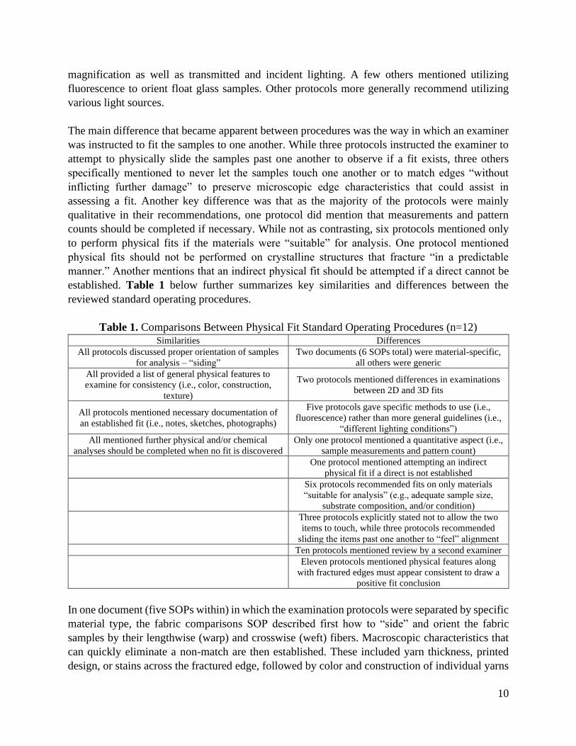
10
magnification as well as transmitted and incident lighting. A few others mentioned utilizing
fluorescence to orient float glass samples. Other protocols more generally recommend utilizing
various light sources.
The main difference that became apparent between procedures was the way in which an examiner
was instructed to fit the samples to one another. While three protocols instructed the examiner to
attempt to physically slide the samples past one another to observe if a fit exists, three others
specifically mentioned to never let the samples touch one another or to match edges “without
inflicting further damage” to preserve microscopic edge characteristics that could assist in
assessing a fit. Another key difference was that as the majority of the protocols were mainly
qualitative in their recommendations, one protocol did mention that measurements and pattern
counts should be completed if necessary. While not as contrasting, six protocols mentioned only
to perform physical fits if the materials were “suitable” for analysis. One protocol mentioned
physical fits should not be performed on crystalline structures that fracture “in a predictable
manner.” Another mentions that an indirect physical fit should be attempted if a direct cannot be
established. Table 1 below further summarizes key similarities and differences between the
reviewed standard operating procedures.
Table 1. Comparisons Between Physical Fit Standard Operating Procedures (n=12) Similarities Differences
All protocols discussed proper orientation of samples
for analysis – “siding”
Two documents (6 SOPs total) were material-specific,
all others were generic
All provided a list of general physical features to
examine for consistency (i.e., color, construction,
texture)
Two protocols mentioned differences in examinations
between 2D and 3D fits
All protocols mentioned necessary documentation of
an established fit (i.e., notes, sketches, photographs)
Five protocols gave specific methods to use (i.e.,
fluorescence) rather than more general guidelines (i.e.,
“different lighting conditions”)
All mentioned further physical and/or chemical
analyses should be completed when no fit is discovered
Only one protocol mentioned a quantitative aspect (i.e.,
sample measurements and pattern count)
One protocol mentioned attempting an indirect
physical fit if a direct is not established
Six protocols recommended fits on only materials
“suitable for analysis” (e.g., adequate sample size,
substrate composition, and/or condition)
Three protocols explicitly stated not to allow the two
items to touch, while three protocols recommended
sliding the items past one another to “feel” alignment
Ten protocols mentioned review by a second examiner
Eleven protocols mentioned physical features along
with fractured edges must appear consistent to draw a
positive fit conclusion
In one document (five SOPs within) in which the examination protocols were separated by specific
material type, the fabric comparisons SOP described first how to “side” and orient the fabric
samples by their lengthwise (warp) and crosswise (weft) fibers. Macroscopic characteristics that
can quickly eliminate a non-match are then established. These included yarn thickness, printed
design, or stains across the fractured edge, followed by color and construction of individual yarns
11
and continuation of the weave/knit pattern. Cordage examinations were established similarly, as
macroscopic characteristics such as width and ply thickness were to be examined first followed by
characteristics of the plastic edges and core fractured ends. The cord should then be opened to lie
flat for examination of the core and allow for examination of core characteristics for compatibility
between pieces when applicable. Another SOP focused on physical fits of polymeric materials.
This SOP recommended to begin with orientation of the samples based on manufacturer markings
or surface anomalies that are consistent across the fractured edges. Along with the overall broken
edges, these distinctive characteristics assist in the establishment of a fit. Along with polymeric
materials in general, an additional SOP was provided for tapes in which instructions are provided
for straightening distorted edges, observing both backing and fabric reinforcement features, as well
as examining any distinguishing characteristics such as backing defects or protruding fabric
reinforcement portions that extend across the fracture. A similar approach was described in the
SOP for paint chip physical fit examinations, in which broken-edge characteristics as well as
surface anomalies are used to establish a fit beyond consistent physical features. An SOP was
provided for physical fits of brittle materials as well. Within this protocol, features due to low and
high velocity impacts, thermal stresses, and bending are described that may become useful in a
physical fit examination.
The second material-specific document consisted of one SOP. This document initially described
differences in observable features in 2D and 3D junctions, providing examples for each. Specific
instructions were then provided for physical fit examinations of fabric and flexible materials such
as tape and other polymeric materials.
Although the majority of reviewed protocols appeared as more generic than material-specific, it is
important to note that a laboratory’s standard operating procedure is a document referenced by
trained examiners during casework. Forensic laboratories have formal training programs
examiners must complete before beginning casework. Specific physical fit techniques are more
thoroughly explained during training, as is evident in a laboratory training guide provided by one
participant. Although this participant had a general physical fit SOP, their physical fit training
manual included detail on specific casting techniques, lighting conditions, and features associated
with fractured items in each of crystalline, amorphous (brittle or plastic), fibrous, and composite
materials. In summary, while this information may not be explicitly stated in an SOP, this does not
necessarily indicate the examiner has never been given more direct instruction.
Although we recognize the sample size is small, the protocol review demonstrated a critical need
to standardize the fracture fit examination methods across laboratories. Currently, there are no
standard guides or standard methods available for the examination of fracture fits of trace
materials. Also, there is lack of specific criteria to support the examiner’s opinion on when the
observed features are substantial enough to conclude a match. Some of the research discussed
below can serve as a basis for the harmonization of procedures and demonstration of validity of
the examinations.
12
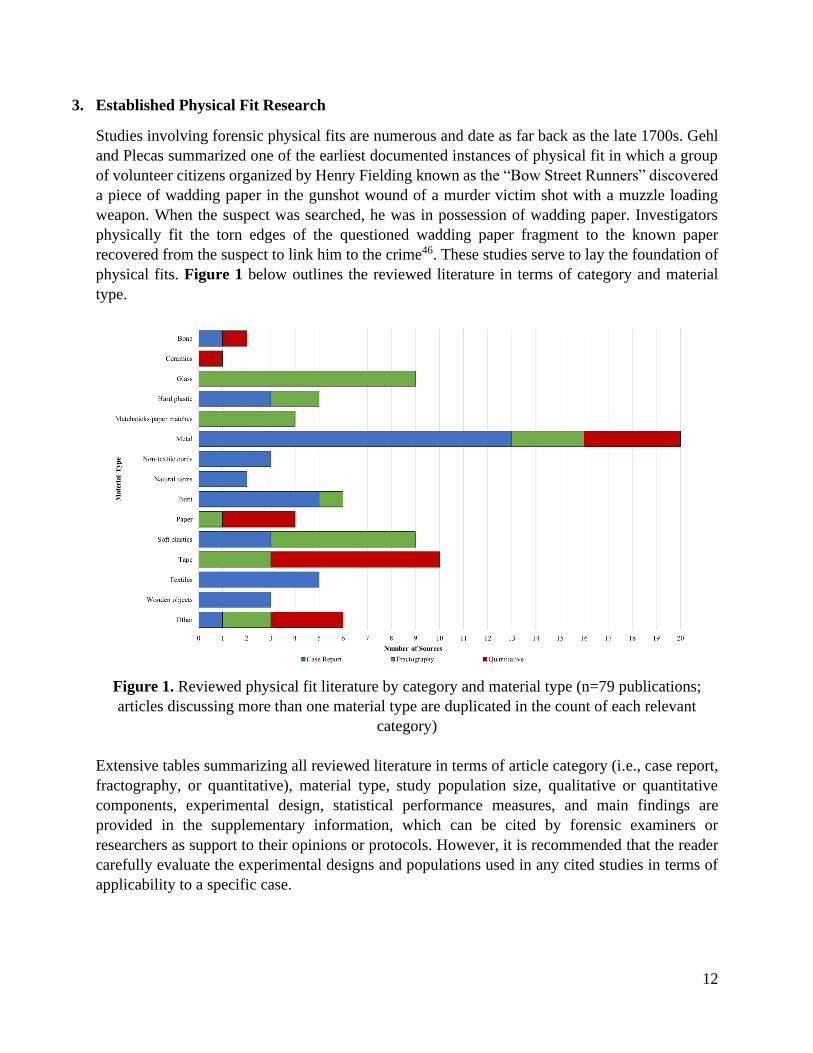
3. Established Physical Fit Research
Studies involving forensic physical fits are numerous and date as far back as the late 1700s. Gehl
and Plecas summarized one of the earliest documented instances of physical fit in which a group
of volunteer citizens organized by Henry Fielding known as the “Bow Street Runners” discovered
a piece of wadding paper in the gunshot wound of a murder victim shot with a muzzle loading
weapon. When the suspect was searched, he was in possession of wadding paper. Investigators
physically fit the torn edges of the questioned wadding paper fragment to the known paper
recovered from the suspect to link him to the crime46. These studies serve to lay the foundation of
physical fits. Figure 1 below outlines the reviewed literature in terms of category and material
type.
Figure 1. Reviewed physical fit literature by category and material type (n=79 publications;
articles discussing more than one material type are duplicated in the count of each relevant
category)
Extensive tables summarizing all reviewed literature in terms of article category (i.e., case report,
fractography, or quantitative), material type, study population size, qualitative or quantitative
components, experimental design, statistical performance measures, and main findings are
provided in the supplementary information, which can be cited by forensic examiners or
researchers as support to their opinions or protocols. However, it is recommended that the reader
carefully evaluate the experimental designs and populations used in any cited studies in terms of
applicability to a specific case.
13
3.1. Case Reports
A majority of early physical fit literature exist as case reports demonstrating noteworthy instances
of physical fit cases in forensic laboratories. These case-based studies have illustrated the
relevance of physical fits in many forensic applications. Currently published case reports represent
a vast array of materials. These include but are not limited to metal, textiles, hard and soft plastics,
paint, wooden objects, non-textile cords, natural items, and other miscellaneous examples.
Existing case reports are described by material below.
3.1.1. Metal
Many articles appear within the firearms and toolmarks discipline, especially in the case of metal
physical fit case reports. For the purposes of this article, the review will focus on realignment of
objects rather than impressions (e.g., toolmarks). To illustrate this, an article by Finkelstein et al.47
described a case in which a seemingly traditional toolmark examination became a physical fit
examination. Toolmark examiners typically associate a tool to a surface by the characteristic
markings imparted on the substrate. In the situation of a forced entry and robbery of a grocery
store, individual markings were not present around the point of entry. However, a small metallic
chip was discovered on the blade of bolt cutters recovered from the suspects' vehicle. This metallic
chip was of similar chemical composition to the material of the fractured padlock, as determined
via X-ray fluorescence (XRF) spectroscopy. Furthermore, the metallic chip appeared to be of
similar morphology to the fractured edge of the padlock. According to manufacturer-provided
hardness values, the bolt cutters theoretically should not have been able to cut a material with the
hardness value of the padlock. Due to this implication, the discovered physical fit was used to
associate two items that otherwise may have been discriminated based on manufacturing
specifications alone47. This study drew attention to a physical fit opportunity that could be
overlooked, and recommended toolmark examiners keep this in mind and work to preserve any
metallic chips found on tools for this purpose.
In many cases, the combination of fractured edge alignment and any manufacturer striations lead
to an association. Tenorio48 provided an example of this through a case report involving an empty
beer can found next to a murder victim and a questioned “pop-top” tab. Comparison microscopy
revealed that striations observed on the tops of both items were in alignment. Additionally, the tab
was flattened and placed in the opening of the beer can, to which the separation patterns aligned
as well48.
It also often occurs that physical fit examinations involve comparison of fracture morphology,
manufacturer striations or features, and striations appearing as a result of use. This scenario
occurred during a case report by Streine49 in which pieces of a knife blade recovered from a crime
scene were compared to determine if they could have originated from the same blade. The pieces
were examined under a microscope. The edges of the pieces were puzzle-like in nature and found
to align with one another. In addition, striated marks both from the manufacturer and those
imparted during use were found to align across the fracture. The discovered striae assisted the
physical fit conclusion49. A similar situation involving striae from both manufacturing and use
14
occurred in a case report by Moran50 in which a victim had broken the suspect’s car antenna from
the vehicle. When observing the two pieces under a comparison microscope, toolmark striations
on the interior of the antenna fragments aligned across the fractured edge, as did external scratches
and markings. While the fractured edges themselves were distorted leading to a limited physical
fit comparison, the presence of the interior and exterior markings added additional value for an
association of the two antenna pieces50.
Another casework scenario involving a knife blade is provided in a case report by McKinstry51. A
questioned, broken knife blade was submitted to the laboratory that had been recovered from the
chest of a stab victim. A month later, investigators submitted a knife with a melted handle and
unknown length of blade apparently missing. The examiner was able to physically fit the broken
blade edges to one another with distinctive fracture edge morphology. Additionally, consistency
between striations present on each blade surface were discovered through a toolmark
examination51.
Karim52 shared a case report involving a broken piece of vehicular tailpipe and alignment assisted
by the manufacturer-sealed seam. In this report, a broken piece of tailpipe was recovered from the
scene of a homicide. Over a year later, a vehicle was recovered with a seemingly broken tailpipe.
The previous piece from the scene was compared to the intact piece on the vehicle for a physical
fit to find that the edges were in alignment despite accumulated mud on the intact piece from
continued use post-crime that was not present on the broken fragment. Additionally, the questioned
piece aligned with a bracket on the tailpipe corresponding to a location with a hook designed to
hold the intact tailpipe in place. The known tailpipe piece was removed from the vehicle for closer
examination of fracture morphology. It was found the pieces aligned with a distinctive separation
pattern and the manufacturer-sealed seam corresponded across both tailpipe pieces52.
Striations imparted to metals due to wear become useful points of comparison during physical fit
examinations. An example of this examination scenario is given in a case report by Reich53 in
which a screwdriver tip was recovered from a door frame in the case of a forced entry. The broken
screwdriver was later discovered in the suspect’s car. Under examination, both the fracture
morphology and use-imparted striae appeared in alignment between the two items53. A similar
examination involving striations was reported by Smith in which a broken antenna fragment from
a hit-and-run was compared via comparison microscopy to the antenna removed from the suspect’s
car. The fractured ends were found to correspond, and linear marks on the outside of the antenna
were found to align across the edges54.
Other physical fits of metals are able to demonstrate alignment through fracture edge morphology
alone. This level of examination is exhibited in several instances throughout the current literature.
Within a case review by Jayaprakash et al.4, one of the reviewed cases described the reconstruction
of a questioned improvised explosive device (IED) tin sheet container and known suspect tin sheet
fragments which revealed a consistency leading to a break-through in the case. In a report by
Streine55, broken pieces of a wheel well were recovered from a homicide scene. The pieces were
later compared to the remaining wheel well of the suspect’s vehicle. Visual alignment was
15
determined between the questioned and known pieces55. Caine et al.56 described a scenario in
which a roof located at a chop shop was physically fit to the roof beams of a known vehicle.
In a case review by Klein et al.57, two cases were presented involving physical fits of bullet
fragments that played crucial roles in their respective investigations. The first case involved a
shooting between gang members. All cartridge casings recovered from the scene appeared to be
of the same type, but investigators wanted to determine if the projectile fragment lodged in the
victim was consistent, meaning fragments found on scene were from the same bullet, fired from
the same gun so as to help establish the number of shooters at the crime scene. Forensic examiners
were asked to compare fragments found at the scene with the one removed from the victim's leg.
A physical fit was crucial for the fragments in this circumstance as the fracture occurred between
land impressions on the bullet, eliminating the possibility of an association due to corresponding
land impressions on each side of the fracture. Through examination under a comparison
microscope and experimentation with several lighting conditions, the examiner was able to
determine a fit existed between two fragments. In the second case, a victim was shot five times by
a suspect wielding two different firearms. Investigators wanted to determine that a third was not
involved. Therefore, bullet fragments found at the scene were again compared to a fragment
recovered from the body. As in the last case example, a land impression comparison was not
possible. A physical fit was determined and agreed upon by an expert hired by the defense
council57.
Robinson58 presented a case report in which a robber assaulted a store owner with a rifle which
then broke into three pieces. The assailant fled the scene with the barreled action and trigger guard.
A suspect rifle was found with a broken trigger guard which was then compared with the recovered
pieces at the scene. Visual alignment was established between the known and questioned pieces.
In addition, surface material on the outside of the trigger guard indicated that the stock was
refinished and the gun reassembled while wet, assisting with the fit assessment58.
An additional case report by Townshend59 involved a slammer tool and two vehicle ignition locks.
The examiner was requested to assess whether or not one of the locks could be identified with an
ignition wing cap found in possession of the suspect. To do so, casts were made of the ignition
lock cores and dusted with gray fingerprint powder to reduce transparency and glare. The cast was
then compared microscopically to the wing cap. Fracture marks on the cast were found to
correspond to one of the ignition locks59.
3.1.2. Textiles
For the purposes of this article, textile materials will include clothing, artistic canvas, shoe insoles,
and rope.
Fisher et al.60 introduced a few examples of textile physical fit cases. For example, a rape case is
described in which a victim cut her hands while reaching for a knife. The suspect tore off a piece
of his shirt to bandage her hands. These fragments from the victim’s hands were later compared to
the suspect’s recovered torn shirt. Another situation was presented in which a hit-and-run victim’s
16
torn coat was compared to a piece of fabric collected from the front fender of the suspect’s car. An
additional scenario provided by the authors involved a torn fabric fragment discovered at the point
of entry of a burglary scene that was later compared to the suspect’s torn clothing60.
Shor et al.61 presented a case in which a physical fit examination was responsible for the
confirmation of stolen artwork. Initially, the only known samples provided to the examiners were
photographs of the original art samples from the owners. Upon examination of the questioned,
stolen paintings, examiners recognized under UV illumination that there had been an over-painting
from the canvas edges to their wooden frames with a brown tint not original to the painting surface.
Examiners removed the questioned paintings from their frames and utilized acetone and glue
remover on the canvas edges to reveal original edges indicating they had been retouched. This
discovery prompted investigators to request the original frames from the owners, from which the
stolen paintings had been cut. Examiners were able to physically fit the cut canvas edges to the
known original frames due to the complex morphology of the distorted canvas61.
Several manuscripts involved an association of separated shoe insole material. An article by Shor
et al.62 presented a case in which an original shoe impression comparison transformed to a physical
fit examination. In this case, castings of three family members' bare feet were made to determine
which of three pairs of shoes belonged to each individual. It was suspected that the insoles of the
three pairs of shoes had been switched in previous examinations within the laboratory. Examiners
were able to discover and document a physical fit about 2 cm long between a questioned insole
and inner shoe bottom. Due to wear pattern, parts of the insole had adhered to the inside of the
shoe, leaving a characteristic contour pattern appearing as mirror images between the insole and
shoe. The fit of the insole fragments remaining inside the shoe to the suspected mislabeled insole
revealed that insoles had in fact been mixed up between shoes previously in the chain of custody.
This case was critical to the authors' laboratory as it led to a protocol change for documentation of
both sides of shoe insoles, to prevent any further misconstruing of evidence62.
In a case report by Laux63, questioned and known rope fragments were compared to one another.
Examination began with a stereomicroscopical examination of the cut edges. The ropes were
examined qualitatively for consistency in color, direction of twist, and comprising material (e.g.,
the rope samples contained two consistent orange fiberglass cords). Quantitative measures were
also employed in the analysis including diameter measurements, number of twists per unit length,
as well as the number of strands, thread, and fibers within the ropes63. While quantitative features
were a part of the analysis, it was not utilized in the physical fit of the inner core.
3.1.3. Hard and soft plastics
In terms of physical fits, polymeric materials are typically classified as soft or brittle in nature. The
nature of the polymer often determines the manner in which it separates and how its pieces are
examined in a forensic context. For example, soft polymeric material typically undergoes an
extrusion process during its manufacture, leaving behind striations that can add a significant point
of comparison during a physical fit examination. This is useful as soft polymeric materials tend to
distort to a greater degree, sometimes limiting comparison of the fractured edge. These
17
characteristics add an additional feature to examine despite edge damage. Alternatively, brittle
polymeric materials often fracture with more distinctive edges, offering more fortuitous
comparison possibilities. Examples of the differences in examination between soft and brittle
polymeric material are provided below.
In a case report by Dillon64, an individual had been suspected of fishing without a license. A fishing
pole with no tackle was found in possession of the suspect. The officer discovered a section of
fishing line on the ground outside the suspect’s car that was connected to baited tackle in the water.
The fishing pole, recovered line, and a knife found in the suspect’s car were submitted to attempt
to see if the fishing line was originally joined. The knife was not found to impart any distinct
features/residues on the line. The lines were severed in one straight pass, and so there were not any
distinct features or irregularities. To examine the thin line, the questioned and known line were
inserted into hypodermic needles to hold the line in place. The examiner observed extrusion striae
patterns in the line that corresponded across the edges. It was concluded that the two sections of
fishing line were once part of the same line64.
Soft polymeric manufacturing features were well established in a case report by Kopec et al.65
involving a homicide case in which a young girl’s body and belongings were recovered in multiple
trash bags. The bags from the scene were submitted for comparison to bags discovered in the
suspect’s possession. Features imparted on trash bags during manufacturing include melt pattern
characteristics such as lines and arrowheads originating due to a mixture of recycled and virgin
polymer pellets in the extrusion process, resulting in varied pigmentation. Transmitted lighting
was used to reveal these characteristic melt markings and striae were contiguous across trash bag
edges, revealing consecutive manufacture65.
A physical fit is presented by Moran66 involved a breaking and entering at a jewelry store. Four
small, black, rubber fragments were recovered from a broken glass doorway. It was noted the
rubber fragments and the rubber part of the bottom of the suspect’s shoes appeared to be of similar
material. Examination under the microscope revealed striations on the surface of the fragments.
Examination of the shoe soles revealed similar striations and missing portions. Direct attempts to
physically match the fragments were inconclusive. The authors then cast the voids in the soles of
the shoes with Mikrosil and compared the casts to the fragments. The casts reproduced the
striations and allowed for comparison of fragment shape and striae. The fragments were ultimately
concluded as having originated from the suspect’s shoes. It was hypothesized that the suspect
kicked the glass door to enter the store, and the broken glass gouged out pieces of the sole,
imparting striations to both the soles and fragments66.
In a case report by White et al.11, examiners received a questioned heel piece and a known suspect
shoe sole from an armed robbery and rape scene. The questioned heel and known sole were initially
aligned by nail hole location and physical size. However, the comparison was enhanced by
examining the heel and sole for fluorescent adhesives. The applied UV-light was able to establish
“excellent points of comparison” between the samples. This report additionally mentioned that
multiple examiners reviewed the match to come to a consensus11.
18
Garcia67 provided an example of a physical fit examination of a brittle polymeric material in a case
report of an individual shot by police. The officer had claimed the individual had threatened him
with two knives. Two knives were recovered from the scene, one of which had a broken handle.
A small piece of material was found embedded in the deceased individual’s hand. The piece was
collected and compared to the broken knife handle to determine if there was support for the victim
carrying the knives. Visual observation revealed that both pieces of known knife handle and the
questioned piece were composed of a similar black, polymer material. In addition, a milling pattern
was seen on the inside of all pieces. The questioned samples and a section of the broken knife
handle were cast using Mikrosil to evaluate a potential physical fit. The cases were found to have
similar features, and when the pieces were directly compared with reverse lighting they were found
to correspond67.
3.1.4. Paint
Paint physical fits may arise in casework through the fracturing of automotive, architectural, or
even safe door paint when tampered with. For example, Osterburg68 presented several examples
of paint chip physical fit cases including corresponding architectural paint chips from a
housebreaking case, paint chips from a burglarized safe, fragments from a torn price tag in
comparison to flaking crow bar paint, as well as a paint chip on a screwdriver head corresponding
to the mold of a door frame68.
Another example of a paint physical fit was presented by Walsh et al.3 regarding paint flakes from
a safe door. In this case, questioned paint flakes were discovered in the suspect’s workshop that
appeared to be consistent with missing paint from six welding beads in the safe door at the crime
scene. Casts were taken of the welding beads and pattern associations were made between the
ridges in the casts and the paint flakes. In this situation, a physical match was made as the welding
ridges were determined to be unique due to the suspected high variability of pattern formation in
the welding process, mainly due to the manual action of a welder along with external factors such
as ambient temperature, metals used, speed of the process, and type of weld3.
An article by Vanhoven et al.69 reviewed two cases where external striations on automotive paint
chips were used to connect questioned paint chips to a vehicle. In both cases, a comparison
microscope was utilized to view the questioned and known fragments of paint. In the first case, a
paint chip collected from a body was found to correspond to a suspect’s vehicle. The fragment
generally fit damage in the fender, only a small section of topcoat remained for realignment. In the
second case, a car struck by a bullet was found to have missing paint on the fender. Paint chips
from the scene were found and compared to the vehicle. In both cases, the external striations were
found to align across the edges of the fragments69.
An interesting paint physical fit case is given in the case review by Jayaprakash et al.4 involved a
stolen van that was suspected of being altered so that its registration details matched that of a
broken-down van. The broken-down van was missing its chassis registration plate, and on the
painted metal surface beneath where the plate was adhered, a trickled, dried paint droplet was
present. An impression of this droplet was discovered on the back of the questioned registration
19
plate on the stolen vehicle. The droplet was found to fit into the impression, and the physical fit
was determined4.
3.1.5. Wooden objects
Physical fit examinations of wood materials are similar to those of metals, as fracture edge
morphology alignment can be complimented by naturally occurring features such as wood grain
and growth rings. This is demonstrated in a case report by Townshend70 in which a large black
walnut tree was stolen. A section of the stump and a wedge piece of wood from the scene was
compared to the end of a tree in possession of the suspects. Examiners observed the grain, rings,
and fracture pattern to determine if the pieces were once joined. It was concluded that the wedge
piece found at the scene aligned to the end of the tree from the suspects. In addition, the examiners
cast a section of the stump and compared the cast to the suspected tree end, finding it to be in
alignment in microscopic features70. A case report by Hathaway71 outlined additional methods that
can be used for wood examinations including xylem and phloem tissue comparisons, along with
the previously established physical fit and growth ring comparisons. In this case, four fragments
of a broken pool cue stick were physically fit together to reveal they were likely once a part of the
same item. The examination was performed in response to a defense attorney’s concern that the
fragments indicated multiple cue sticks were involved in the homicide under investigation71.
It is common in case reports that along with presenting their evidential findings, authors share a
useful technique that assisted in optimal demonstration of alignment, or the typical methodology
they tend to follow in their examinations. In a case report by Christophe et al.72, the authors
exhibited how they were able to utilize Photoshop techniques to best visualize a physical fit of a
questioned wood chip to a damaged wooden pallet. The described scenario involved a hit-and-run
in which the suspect was carrying a wooden pallet in the back of his truck. A wood chip was
discovered at the scene. The questioned fragment was scanned with a high-quality photo-scanner,
enhanced, and overlaid to a scan of the known pallet section. Markers were used to highlight points
of significance along the corresponding fractured edges for illustration to the jury72.
3.1.6. Non-textile cords
Cable or wire physical fit examinations often involve a comparison of multiple material types on
the fractured edge, as most cabling consists of a metal core and polymeric outer insulation material.
An example of this is provided in a case report by Kenny73 of a stolen truck radio. The stolen radio
was recovered from a group of suspects, and the victim was unable to positively identify the radio.
The radio was then submitted to the laboratory for a physical fit comparison between the severed
wires on the questioned radio to those remaining in the victim’s vehicle. Visual observation of the
wires revealed air pockets in the insulation layer of the wires, present in the severed edges of both
the known and questioned samples. The air pockets were determined to correspond across the
fractured edge73. A similar examination is presented by Striupaitis74 in which eight sections of
cable were received from a theft from a public utility company. Law enforcement submitted these
wire pieces in cut portions: two standard portions from the scene and six portions from the
suspects. To look for a fit, the examiner cut the sections horizontally in order to lay the material
flat and examine the entire fractured edge at once. The examiner was able to observe a fit between
20
one of the standard sections and one of the evidence sections on the outer layer of the wire. In
addition, the examiner was able to observe an inner layer of the wire with printed wording that
also aligned74.
3.1.7. Natural items
Interesting case reports involving physical fits of biological materials are also provided in the
literature. Examples include those of skin and fingernails, as described in publications by Perper
et al.6 and Bisbing et al.7, respectively. In the case of the skin physical fit, a questioned skin sample
discovered at the crime scene appeared consistent to a known injury on the suspect’s thumb. The
examination consisted of overlaying the questioned skin on the known injury for observation as
well as fingerprinting the questioned and known sample for assessment of friction ridge
consistency. Serological testing was also performed on both samples, and the authors claim this
factor is an objective support to any subjectivity of their physical fit examination6. In another
instance of a physical fit, examiners received a questioned fingernail fragment from the crime
scene that appeared consistent with the damaged edge of one of the suspect’s nails. A clipping was
taken for a known sample and the grooves in the nail plate between the two samples were examined
for alignment under the microscope. As the basis for the individuality of one’s fingernail grooves
was not established, examiners reported the match as probable rather than definitive7.
3.1.8. Other
Unconventional methods of physical fit involve overlays of digital images to best visualize
alignment. Another case shared in the Jayaprakash et al.4 case review was an interesting
application of physical fit in which an unidentified body was determined to be that of a missing
child due to consistencies in suture pattern and contour of the Wormian bone in the skull through
comparison of the questioned skull and known victim ante-mortem x-rays. The fit was crucial in
this case, as DNA analysis was impossible due to decay of the body. Another case in Jayaprakash
et al. involved another identity determination in which video superimposition of known victim
facial footage and a questioned skull from an unidentified body were compared. The alignment of
dentition led to a positive conclusion. This review article, while also pointing out unique
applications of forensic physical fits, also discussed one of the key limitations of this type of
research - that probabilistic statements regarding physical fit are challenging due to variable
circumstances surrounding the match “population”, as materials and events surrounding the
fracture vary on a case-by-case basis4.
3.1.9. Summary
Case reports are well established in the literature, as evident in the large portion of case reports
reviewed in this paper as shown in Figure 1. Despite their vast presence, it is critical that physical
fit case reports continually be published to allow the documentation of the types of materials
received in crime laboratories to stay current. These reports provide an important knowledge base
regarding the presence of distinctive features along fractures of various substrates, as well as
demonstrate to researchers the vast array of unusual circumstances in which physical fit cases arise
in forensic laboratories. Through reviewing case reports, researchers gain a better understanding
21
of prevalent materials and features from which to base their research on in order to best assist,
support, and advance the discipline.
In addition, while case reports tended to thoroughly explain the circumstances of the case as well
as the examination results, few detailed the methodology used to come to their conclusions.
Examiners publishing future case reports might consider describing their basis and rationale for
their decision-making and fracture edge feature interpretation processes to better inform the end-
users. Further, the majority of case reports reviewed in this paper were based on metallic evidential
materials. In order to provide a better understanding of frequent physical fit examinations
performed in forensic laboratories, there is a need for increased publication of case reports for
physical fit examinations for other material types often received in trace evidence units.
However, due to the limited nature of evidential samples, case reports unavoidably are based upon
a limited sample size and rarely can report statistical performance rates of the physical fit analyses.
This illustrates the importance of research studies establishing large population sample sets from
which probabilistic interpretations can be made, to provide reference and support for forensic
examiners when working with similar material types. Therefore, while it is crucial for forensic
examiners to publish their experiences to establish the realistic state of evidence received in the
field, it is equally important for researchers to educate themselves on the prevalence of material
types in casework and take their findings into account with their experimental designs. The close
collaboration of academia, researchers, law enforcement personnel, and practitioners is vital for
the advancement of the discipline. Also, due to the large variety of materials processed for fracture
fit analysis, a multi-disciplinary approach to evaluation of casework items would be beneficial.
3.2. Fractography and Qualitative-Based Studies
Existing forensic fractography studies aim to understand the mechanism of the fracture as well as
to determine the source of damage (whether it be shearing, tearing, sawing, etc.) based on
morphological characteristics. These studies establish features due to the fracture morphology for
qualitative-based comparison techniques. A variety of fractography-based studies exist for
materials including hard and soft plastics, glass, matchsticks and paper matches, metal, paper,
paint, and other miscellaneous items, listed in decreasing quantity.
The nature of fracturing, features, and methods of evaluation, especially for brittle materials such
as glass, are covered in fractography textbooks and practice guides75,76. Fréchette75 discussed the
fundamental markings on cracked surfaces by initially explaining the concept of the origin flaw,
the flaw or discontinuity in a brittle solid surface from which cracking begins. The origin flaw can
be imparted on a material by chemical, thermal, or mechanical means. Cracks propagate by
forming a new surface perpendicular to the axis of principal tension, beginning at the origin flaw.
The more stress applied at the origin flaw, the quicker the crack will propagate. At any point during
crack propagation, an external influence may cause a change in direction of the axis of principal
tension, resulting in an alteration to the morphology of the running crack front. Events such as this
influence the variability of a resulting fracture pattern75. Quinn further discussed the origin of
22
different fractures, including whether or not pre-existing flaws that contribute to fractures are a
result of external manufacturing (extrinsic), or are a result of the internal structure of the material
(intrinsic)76.
Fréchette75 also described the types of markings that can result in brittle materials from fractures,
starting with the rib and hackle markings imparted in glass. The author highlighted markings found
within the rib mark family (markings concave in the direction from which the crack came from)
including arrest lines, three types of Wallner lines, and scarps. For a more extensive description of
these fracture details, the reader can refer to Fréchette75.
The literature also discusses how features in brittle materials can lead to fracture variability.
Fréchette stated that inclusions in brittle materials are subject to spontaneous cracking during a
fracture event as in wake hackle, for example. Inclusions also lead to crack variability as cracks
tend to deviate from the axis of principal tension in order to avoid intersecting with an inclusion
under tensile stress, in turn tending to intersect with inclusions under compression75.
Quinn’s practice guide highlighted common tools and instruments that can be used to examine
fractures. Jewelers’ loupes and various microscopes allow for closer magnification of overall
fracture structure, while instruments such as scanning electron microscopy, confocal microscopy,
and X-ray topography can be utilized to observe obscure features or perform chemical analysis on
the material76.
3.2.1. Hard and soft plastics
In terms of polymeric material, fractography studies tend to examine the fracture mechanisms of
brittle materials and report techniques for best handling and visualization of soft fractured
materials for purposes of physical fit examination. For example, within a study on fracturing of
various materials by Katterwe77, polymethyl methacrylate (PMMA) sheet fractures were studied.
Fracturing occurred using an impact “hail-stone gun”. Plastic balls of two different sizes (20- and
40-mm diameter) were discharged at the PMMA sheets. The velocity of the balls was measured to
determine the kinetic energy of each fired projectile. The cracks from the impact revealed that
fracture features varied even when struck with plastic balls at the same kinetic energy, revealing
the characteristic nature of polymeric fracture surfaces77.
Studies suggesting methodology to best handle fractured soft polymeric materials often occur for
tapes and plastic bags. For example, an article by Weimar78 demonstrated a method for reducing
distortion or stretching on the edges of PVC-tapes (electrical tapes). Tapes from six different
manufacturers were torn by hand and their ends were observed with a comparison microscope.
The edges were then treated with 100°C hot air for a few seconds. This temperature was chosen to
prevent melting of polyvinyl chloride often used in the tape backings. After treatment, the tapes
were re-observed under comparison microscopy. The heat treatment was found to make it easier
to find the corresponding edge, and to improve examiner confidence in the conclusion. The author
did note however that applying heat treatment may destroy other evidence such as DNA or
fingerprints78.
23
Specific methodology is also established for the comparison of castings of electrical tape ends in
a study by Weimar79. Tape samples were either sheared or torn for the creation of match pairs. In
order to obtain castings, tape ends were heat-treated at 100°C with demineralized water to undo
any plastic deformation occurring after the fracture. Ends were then able to be recreated with
casting material. Corresponding end casting pairs were examined under a comparison microscope
for the fracture matching process. The author concluded that each fracture cast generated a
distinctive pattern for nearly mirror-image comparison microscopy results79.
While technically a case report, a fractography study was completed within a publication by Agron
et al.80, in which the authors described their process of recreating electrical tape fracture pairs to
demonstrate distinctiveness. The recreated fractures were used to support their determined
physical fit in an investigation of an explosion involving a hand grenade. Various examples of torn
and sheared electrical tape samples were photographed to provide a demonstration to the jury of
distinguishing features along the fractures80.
Comparably, a study by von Bremen et al.12 proposed criteria for revealing sequential relationships
in plastic garbage and sandwich bags. Bags were purchased from various local retailers as well as
known consecutive samples obtained from manufacturing plants. Recommended comparison
points were mainly qualitative regarding bag color, size, perforations, construction, and any
colored individual striations including fisheyes, arrowheads, streaks, and tiger stripes. These
individual pigmentation characteristics can be viewed utilizing polarized light microscopy. The
authors did introduce a quantitative factor for consecutive manufacture determination. This
involved calculating the slope of any prominent markings present across all known consecutive
bags. Slope was ranked increasingly to determine sequence of manufacture. Questioned samples
obtained from the same manufacturer could then be used to determine the number of missing bags
in the sequence by taking the difference of the height of the striation on the questioned bag and the
highest known sample, then comparing this value to the average height of the known sample
striations12.
Vanderkolk81 published a similar article regarding the determination of consecutively
manufactured garbage bags; however, the article was an illustrative review of methodology and
general features to observe during an examination rather than a study involving physical samples.
Alignment was recommended according to the heat-sealed edges of the bags. Striations imparted
during the manufacturing process, as those described by von Bremen et al.12, can be visualized by
transmitted light beneath the sample and used to make a physical fit81.The different types of
markings that can be used to establish sequential relationships in plastic films were also
demonstrated in an article by Pierce82. The pigmentation in these additives create patterning or
striations that can be used to fit films together to reveal sequential relationships. The article also
mentioned these additives can cause abrasion to production machinery, leading to differences in
film perforations, cut edges, and roller imprints82.
24
Denton83 shared in a similar article a method for photographing extrusion marks in polyethylene
films. As discussed previously, extrusion marks are left behind as a result of debris on the extrusion
die in the manufacturing process. The marks are discontinuous, and so therefore can be used to
assist fracture matching across consecutive bags. To photograph them, a black card was cut to have
⅛ inch x 6 ½ inch slots. Two sheets of glass were put together and placed above the grid. The grid
was illuminated by a 500-watt lamp at a right angle. Extraneous light was reduced by a black
shield. The camera was focused on the glass in the frame so that the whole area of glass would be
in the negative. The piece of polyethylene was sandwiched between the glass sheets with the
extrusion marks on the short side. The authors found this set up allowed them to optimally capture
the extrusion marks83.
Ford84 provided an additional article establishing methods to best photograph features for
comparison of plastic bags and film that have potential to be used to denote matching edges or
connected pieces of evidence. Extrusion marks were recommended to be photographed using a
secondary lens system so that the extrusion marks can be focused at any magnification. Heat marks
originate from bags that are sealed together by an individual separately from the manufacturing
heat seals. Secondary heat marks were often created using a soldering iron or laundry iron, or by
commercially made sealing machines. For sealing machines, conclusions were made by examining
the patterns left by the heat proof fabric on the machine, by observing inclusions and irregularities
created in consecutive seals made by the same machine, and by hot spots (unique areas of
deformation caused by heat). Cut edges of films offered some additional details if the instrument
used to sever the edges left similar characteristics (snags, changes in direction of cut, etc.)84.
While multiple articles establish methodology for the comparison of plastic bags and films, an
article by Castle et al.85 provided a summary of a variety of methods that can be used to visualize
and assess physical properties of plastic bags and cling film. In addition, it also summarized the
manufacturing of plastic bags and film. In short, three methods were provided for feature
visualization such as color and variation of die lines, polarization patterns, and striations from
manufacturing. These methods included utilization of a polarization table,
shadowgraphy/Schlieren imaging, and incident/transmitted light microscopy. The article also
provided four case examples in which these methods proved useful in the analysis of polymeric
materials. For further detail on the use of these methods, refer to Castle et al. 85.
3.2.2. Glass
Numerous articles exist in forensic literature discussing the fracturing mechanics of glass as well
as resulting patterns. A study by McJunkins et al.86 described multiple experiments in which glass
is fractured, focusing more on the mechanism by which the glass fractures rather than the process
of fitting samples back together. The article described the two major types of glass fracture patterns
– radial and concentric patterns. The article also described the appearance of fracture patterns when
a bullet has travelled through safety or tempered glass - the entrance plane of the glass bullet hole
will exhibit perpendicular chips while the bullet exit plane will show angled chips on the glass86.
25
Another glass fractography study was completed by Harshey et al.87 through the analysis of
fracture patterns made in glass from a projectile fired from an air rifle. The authors fired a 4.5 mm
air rifle at windowpanes with three different thicknesses. Each type of windowpane was available
with and without sun control film (SCF). They then recorded various measurements on the fracture
patterns including radial fracture count, concentric fracture count, bullet hole diameter, mist zone
thickness, and mist zone diameter. Generally, more radial fractures were observed than concentric
in each of the glass types. It was determined through the chi-squared test that no significant
differences were present in fracture pattern measurements between the thicknesses, regardless of
SCF.
A study by Thornton et al.88 described glass fractures occurring due to being shot with projectiles
in which there is no obvious distortion. Characteristic striations occur under quasi-static loading.
In essence, the fracture occurs when the glass fails at a Griffith crack, minute flaws that are often
a point of stress concentration. The author’s goal was to demonstrate that glass can break under
tension even if deformation is not visible. This is described in terms of dynamic loading through
the projectile and mechanical waves that propagate through glass when shot. These waves have
enough stress to produce a crater in the glass even if the projectile does not cause full penetration.
For further information on this phenomenon, refer to Thornton et al. 88.
An extensive glass fractography study is provided by Baca et al.89,90 in which the researchers
fractured 60 replicates each of double strength glass windowpanes, wine bottles, and taillight
lenses. Both dynamic and static impact fracturing devices in controlled conditions were utilized.
Of the glass samples, the 60 8x8 inch windowpane fragments were all cut from the same sheet of
glass, and all wine bottles were donated from the manufacturer, all taken from the production line
on the same day. This was done to assure all samples originated from the same batch. For dynamic
impact, a device was constructed utilizing a drop weight at adjustable heights to initiate fracture
through an attached indenter tip without penetrating the sample. Static impact was applied through
compression with a tensile tester also fitted with indenter tips. Each experiment used three indenter
tips interchangeably – a sharp tip, a round tip, and a blunt tip. Of the plastic samples, polymeric
taillight lens covers of the same brand and part number were utilized. Indenter tips differed for the
polymeric samples as sufficient velocity to break the samples with the previously used tips could
not be obtained. Indenter tips consisted of a 2-inch diameter flat disc for the static impact tests.
For polymeric dynamic impact tests, a dropping pipe device was used that is typically used to
induce filament deformation in automotive lamps. Fracture velocities were measured using both a
video of the event analyzed in MATLAB software as well as wavelength sensors and a timing
mechanism. Maximum extension and maximum load value determinations were also recorded.
After fracturing, samples were reassembled and covered with clear tape for ease of fracture
morphology documentation via hand-sketching, scanning, and digital CAD representation by
tablet drawing. Fracture patterns were compared by overlay to all other fracture patterns within
their respective sample type. This led to a total of 5,310 pairwise comparisons over all sample sets.
Visual examinations were reported to reveal differentiable fracture patterns between similar
samples under reproducible conditions. It was also observed the blunt fracture tips typically
required the most velocity and load to initiate a fracture, while the round tips required the least.
26
This reflected in the number of fracture lines, as the tips requiring the highest velocity imparted
the most fracture lines on the sample89,90.
A similar fractography study is provided by Katterwe77 in which reproducible fracturing of glass
was examined for variation in fracture morphology. In a static fracture experiment, small slides of
plate glass were used in conjunction with three different loads, represented in units of Newtons
(N): 0.98 N, 2.0 N, and 2.9 N. A hard indenter was used to apply each load, creating fractures in a
reproducible fashion. The fractures were found to have random distributions of cracks. The cracks
themselves were found to be in random quantities, lengths, propagations, directions, shapes, and
orientations. The second part of the study was bending of glass, in which a universal testing
machine was used to create reproducible load distributions. The resulting curves and fractures were
also randomly distributed, illustrating the distinctive nature of glass fracture77.
Nelson9 described qualitative features that can be used to exhibit glass fragment alignment,
referencing a recent hit-and-run case. The author first described the two types of glass fracture
markings that can be utilized for this purpose. These included rib markings, those appearing as
oyster shell-like fractures, and hackle markings, appearing as small striae normal to rib markings.
Hackle markings were found to be most useful for alignment. The method the authors
demonstrated for glass physical fits was facilitated by placing a convex glass chip into its original,
concave medium and viewing alignment under the microscope through the chip surface, normal
to the fracture. It was recommended to photograph the fit with surfaces aligned as well as slightly
displaced, so hackle marks were revealed. The author referenced a hit-and-run case in which this
method was applied, placing two 3/8 inch glass fragments within larger broken headlamp
fragments to identify corresponding features9.
Glass fractography features useful for examination purposes are further explored in Thornton’s
chapter of “Forensic Examination of Glass and Paint: Analysis and Interpretation”91. In his chapter,
noted methods beyond traditional aligning of irregular surfaces included microscopic alignment
of rib or hackle marks, identification of continuous ream or cord via shadowgraph, and
visualization of surface irregularities through laser interferometry. Ream is the typical term for
these markings in sheet glass while cord is used for container glass. Ream (or cord) are markings
imparted due to physical and chemical property variations within the glass, potentially forming
due to poor melting and batch separation within the furnace at the manufacturing plant92. These
additional techniques arise due to the three-dimensional nature of glass physical fit. Thornton also
established the random formation of glass fractures by explaining how fractures propagate through
the randomly oriented crystal lattice composing glassy materials. He claimed this understanding
provides a “universal acceptance of the uniqueness of a match”91.
Indirect glass physical fit is explored in a study by von Bremen92. Within the article, the author
described a method utilizing ream or cord markings to establish associations between non-
contiguous glass fragments. These markings appear as striations within the glass and were
visualized in the article by shadowgraph photography. This method involved placing photographic
film beneath a glass sample and placing a light source above it to cast a shadow onto the film. The
27
shadow pattern was developed as a photograph that allowed visualization of any ream of cord
markings. Along with sheet glass, von Bremen also examined 14 glass bottles for cord, which was
identified in all samples with varying patterns between bottles. Shadowgraphs were also used to
image patterns of six transparent plastic samples and five automotive bulbs. After demonstrating
successful images produced via shadowgraph, von Bremen outlined a study utilizing window glass
obtained from a known manufacturer to examine the frequency and persistence of ream markings.
Four sheets of glass were used to create 1.8-cm wide strips examined in various combinations of
non-contiguous distances between one another. Twenty-one strips were examined that originated
1.8-cm apart in the original sheet, 12 were examined at the 13-cm distance, and the two extreme
edges of each glass sheet were used to compare strips 70-cm apart. 90% of ream marks persisted
at 1.8-cm, 33% persisted at 13-cm, 10% persisted over 70 cm, and at 140 cm none were identified
as matching. From these results, von Bremen demonstrated that ream can be used to associate two
sheet glass fragments even when a direct physical match is not present92.
3.2.3. Matchsticks and paper matches
Many fractography articles involving matchsticks share specific techniques that may assist in
visualizing qualitative features during examination, such as the method reported by Gerhart et al.93
involving matchstick to match book comparisons. Suspected match to matchbook samples were
first compared for size, color, wax dip line, and cut or torn edges. The samples were then
submerged in a high refractive index liquid in order to make the cellulosic surface fibers of the
matchsticks transparent, to allow for ease of viewing further fracture edge detail. The authors
claimed this approach has proven highly effective in roughly 40 casework comparisons through
the years93. In another article involving the comparison of match sticks and booklets, Funk10
described a method used to establish consistencies between matchsticks as tested on eight total
booklets: four Canadian, two American, one Brazilian, and one Japanese in manufacture. The
method was similar in that the surface fiber continuations across consecutive matches are being
examined, however the technique used involved dyeing the matchsticks via stain on a wooden
roller, mounting the dyed matches on wooden blocks, and examining them under both stereo and
comparison microscopes. The authors concluded this method is reliable, cheap, easy, and effective
as they claimed the technique has yet to be reported to cause false positives10.
An additional method for examination of paper match sticks was presented by von Bremen94
utilizing laser excited luminescence. In this study, match boards were removed from books and
both surfaces of book were searched for luminescing inclusions and fibers. The manufacturer-cut
sides of 120 matches from 6 books were searched for inclusions with stereomicroscope. During
both search types, both an argon and dye laser were used for illumination. Images were taken of
all observed inclusions. Results showed that the argon laser produced more luminescing inclusions
than the dye laser, even though the dye laser seemed to excite more fibers. Although the dye laser
was able to reveal some inclusions that were not shown by the argon laser, the argon still performed
optimally. The dye laser also had the capability to show cross-sections of a single fiber94.
In a study by Dixon, the author provided a recommendation for the minimum number of features
to be determined consistent for a positive fit conclusion95. Dixon first highlighted ten major points
of comparison in analysis of torn or burned matchstick fragments. These included the length,
28
width, thickness, waxing, color and thickness of coloring material, the fluorescence of filler
materials or sizing, cut edges, torn edges, inclusions, and cross-cut and torn fiber relationships,
both horizontal and vertical. The author provided the recommendation that a minimum of four
cross-cut or torn fibers must be associated using these comparative points between the questioned
and known samples for a positive identification, but only if the match head is still intact95. This
provided a basis for consideration of comparison requirements.
3.2.4. Metal
Fractography studies for metals consist of breaking source determination studies as well as studies
looking into the fracture edge variation of metallic materials. These studies examine the
morphology changes in their respective matrices in a fracturing event, which provides an important
foundation to the understanding of physical fits. In a study by Matricardi et al.96, various metal
wires were fractured through five methods including tension, shearing, torsion, diagonal cutting
and sawing. Their respective ends were then compared via Scanning Electron Microscopy (SEM)
to determine if fracture source could be attributed from the cross-sectional shapes. The authors
reported that “sufficient detail” for breaking source determination was shown in the tension,
torsion, and diagonally cut wires, but not in the sheared samples96.
Another fractography study considering wires is that of Katterwe77, which was completed to study
the variation of fractured wire edges. Tensile tests were performed on steel wires until failure was
achieved. The steel wires were found to allow for a fracture match between the edges. The curves
and fracture surfaces were random and varied between the different wires, despite being made of
the same material77.
In addition to studying the way in which materials fracture, many studies then include qualitative-
based reporting to highlight features resulting from the fracture that can be used by the examiner
to illustrate that two items were once part of the same object. A study of this type was completed
for metal keys by Miller et al.97 in which six sample sets of five keys each were broken either by
bending or sharp impact. Known matches were first microscopically examined and photographed
to demonstrate distinctive features, followed by a verification that known non-match pairs did not
appear consistent due to similar features. Examinations were completed in the following sequence.
The overall fit pattern was first observed for alignment, followed by the correspondence of the
toolmarks across the fracture as subclass characteristics. Scientists then examined the internal
fracture pattern, making note of any abstract features, ridges, or furrows consistent across both
samples through observation under a comparison microscope. By propagating their analyses in
this manner, the authors concluded that known match pairs appeared to share a high level of
agreement based on qualitative features97.
3.2.5. Paper
An article by Barton98 described a method for more efficient visualization of paper delamination,
the unequal tearing of paper layers. This method was discovered during a typical electrostatic
detection apparatus (ESDA) analysis for writing impressions on a torn piece of document paper
and was later studied through examiner-torn paper. When the torn papers were placed into the
29
ESDA with their delaminated edges facing up, the delaminated regions appeared dark in contrast
to the remainder of the page in the resulting ESDA image. This technique was useful for rapid
visualization of corresponding paper tears and was not affected by the routine humidification
imparted on paper being examined for writing indentations98.
3.2.6. Paint
A study to determine a method for association of separated vehicle parts was shared by Gummer
et al.14 Through their research, door hinges were examined qualitatively to determine if matches
could be established between a vehicle’s driver-side door and hinges by the patterns associated to
each. Patterns formed between door and hinge as any gaps between the panels allowed capillaries
to form in the surface coating of the paint. This caused striations to form that could assist in
alignment. Six vehicles of two models were examined, both Ford Telstars and Ford Lasers. Two
points of contact of the hinge in the driver’s door were analyzed. The authors found that surface
coating striations were distinguishable between vehicles. However, if electro-coating between
panels was poor, these patterns would not appear at all. 14. This study revealed a unique method of
establishing alignment between vehicular door panels and door hinges.
3.2.7. Other
A method meant to be applied to many fractured material types was provided in a review article
by Zieglar99. The article highlighted two optical techniques to aid in comparing fractures when one
is a mirror/negative of the other. Under most cases, overlays would be done using photographic
overlays or surface molds, but often detail is lost. The two optical techniques highlighted by the
author are a beam splitter technique and reverse lighting. Beam splitters are optical devices
designed to split light in half, one portion being reflected, and the other being transmitted. The
divided light allowed the observer to examine the object directly and/or a reflected image of the
object. Beam splitting helped with recessed fractures and allowed for an overlay. Reverse lighting
inverted the surface of one object being examined and could be used correspondingly with beam
splitting. These methods allowed for an easier examination of difficult fractures, either by the
nature of the fracture or by highlighting features that would be lost under standard comparison
microscopy techniques99.
3.2.8. Summary
As shown above, fractography studies provide a deeper look into the specific features that may
assist in assessing a potential physical fit between two fractured items. Studies involving controlled
fracture of various materials for assessment of any resulting features, as well as studies outlining
a methodology for best contrast and visualization of alignment features are critical to the forensic
science community. These studies assist forensic practitioners in sharing alternate viewpoints for
assessing certain material types and assist researchers in understanding the features considered by
examiners to evaluate a physical fit. Further, studies initiating controlled fractures provide an
essential foundation for the knowledge of the separation tendencies of specific material types. By
observing the fracturing process, researchers understand the development of features that may be
useful in the alignment of separated items. For the physical fit discipline to progress, more
fractography studies must be initiated, attempting to understand fracture mechanisms and the
30
features imparted to the items during the separation or fracture of the materials. Practitioners must
also continue to share their comparison processes to facilitate further conversation and consensus
into the decision-making involved in physical fit examinations. Determining which fracture
features are class characteristics and which are distinct has not been specifically addressed in a
consensus-based protocol. One reason may be that it depends on each material’s physical and
chemical properties. This remains by far one of the main challenges towards the harmonization of
decision-making in current practice. Studies based on fractography, provide a body of knowledge
to set the basis of such comparison criteria.
3.3. Quantitative Assessments of Physical Fits
3.3.1. Performance rates
Studies observing performance of methods to compare fractured items utilize validation sets in
which the true origin of the samples (the original matching piece) is known. To mitigate bias,
examiners usually remain blind to the origin of the samples during the comparisons. When utilizing
validation sets, four outcomes can be identified. A true positive is an outcome where the examiner
correctly identifies as a match a pair of items that originated from the same piece. A true negative
result is when the examiner correctly reports the pair as a non-match when the items originate from
different pieces or objects. False negatives result when the examiner incorrectly reports a pair that
was once the same piece as a non-match. A false positive is the outcome when an examiner
incorrectly reports a match between objects originating from different items or pieces. In addition
to those outcomes, some studies also separate misidentifications - false positives and negatives -
from inconclusive results, in which there were not enough distinct features for the examiner to
reach a conclusion of match or non-match. Performance rates such as sensitivity, specificity and
accuracy can be calculated based on the results of the validation sets. Sensitivity, or the true
positive rate, is the number of true positive pairs out of the total number known matching pairs in
the set. Specificity, or the true negative rate, is the number of true negative pairs out of the all the
known non-matching pairs. Accuracy would be calculated by the total number of true positive and
true negative pairs out of all the pairs in the set.
Physical fit literature involving performance-based assessment includes materials such as bones,
metal-coated papers and silicon cast sheeting, metals, and polymeric material including tapes. In
a study by Christensen et al.15, volunteer examiners performed physical fit comparisons of various
bone, shell, and tooth fragments. Overall, the positive association rate was found to be 92.5% with
only four negative associations reported at a rate of 0.1%15. Performance rates were also evaluated
for metal-coated papers and silicon cast sheeting in a study by Tsach et al.16 in which samples
were torn on a tensile machine and a double-blind physical fit analysis was performed. Of the 24
fracture pairs examined, all were correctly matched for the entire length of the fracture. Twelve of
the pairs were attempted to be matched according to transparencies of only 1 cm of the fracture
edge. Of these, 66% were correctly identified. When examiners were provided with the actual
materials for analysis rather than transparencies, all were correctly identified at 1 cm16.
31
Performance rates were examined for the comparison of hacksaw blade physical fits in an article
provided by Claytor et al.100 This study was conducted to look at the fracturing of metal using a
repeatable technique. The authors used a measuring software to document fracture characteristics
and also conducted a proficiency test of the comparison process. Twelve consecutively
manufactured hacksaw blades were used. Two blades (A and B) were labeled at 1-inch segments
(e.g. A1-A22) and broken into 12-inch segments. A cast was made of each evenly numbered edge.
Images were taken of each edge, and then the odd edges were compared to every even edge and
documented. To conduct the proficiency tests, four consecutively manufactured blades were
broken in the same manner, casts of the edges were taken, and all the items were labeled with a
test number and item number. 253 comparisons were made using A and B (33 within each blade,
and 187 between). The authors found more points of alignment using topographical evaluation of
the edges compared to the physical fit of the edges. Of the proficiency testing, 330 test results were
returned. 157 of 173 true matches were reported (90.8%). 109 out of 157 true negatives were
reported (69.4%). If inconclusive results were included, the true negative rate increases to 98%
(154/157)100.
A study by Orench18 attempted to demonstrate the high degree of variability possible in the fracture
patterns of metals. The authors first established the potential for variation by describing the way
in which metal specimens fail. When a load applied in either tension, compression, shear, torsion,
or bending was applied to a metal, it in turn experiences a strain due to planes of atoms moving
relative to each other, known as dislocation movement. Crystal morphology of the metal alters the
way in which dislocation occurs. Fracture morphology will change at areas of crystal imperfections
known generally as point defects, line defects, planar defects, and bulk defects. Within these
categories are 15 types of defects, meaning any given grain of a metal can have any number or
combination of these defects. This allows for great variability in the overall fractured edge,
increasing with fracture length. Possibilities increase even further when considering the five load
types that may be applied in any given combination. The aim of this study was to provide error
rate data specifically dealing with metal fracture to conform to Daubert criteria. Twenty sample
sets of ten 0.25-inch diameter steel fracture fragments each were created. A random number
generator was used to select a three-digit number to engrave on the end of each piece to mark a
true match pair. Fracture fragments were established by notching each original sample 50% of its
diameter halfway down their length with a diamond cutter and pulling them apart with a tensile
tester. Of each sample set, two of the ten fragments were true non-matches to all other possible
ends in the set. Ten examiners participated in the blind comparison process. Each was randomly
assigned two sample sets to complete. Examination followed typical comparison procedure via a
comparison microscope with a digital camera and fluorescent light source. All examiners had a
100% success rate with no false positives reported. This study indicates the high variability of
metal fracture morphology leading to high success in metal fracture fit examinations18.
The correct association rates of duct tape fracture fits were assessed in a study by Bradley et al.17
in which four examiners performed fracture fit analyses on five comparison sets, three of which
were hand torn and two were scissor cut. The authors reported that 92% of hand torn samples and
81% of scissor cut were correctly identified. No false positives or false negatives occurred; the
32
remaining fraction of pairs were reported as inconclusive. When examiners were asked to re-
examine the scissor cut set due to the lower matching percentage, two misidentifications did occur.
The authors also stressed the importance of the peer review process in these types of
comparisons17.
In an additional study by Bradley et al.101, the association rates of electrical tape end matches were
examined. Three examiners performed end matches on 10 sets each of electrical tape fracture pairs
created from 7 rolls of constant color and width. Each set design consisted of factor variation
between tape brand, test set preparer, and mode of separation (tear, nick then tear, and dispenser-
torn). Between the 30 total test sets distributed, a total of 2142 end comparisons were possible due
to various combinations of tape ends. Of these, 106 known end matches existed of which 98 were
correctly identified. Of the remaining pairs, 7 were inconclusive and one was a false positive. A
secondary reviewer also reported a false positive on the same tape pair. Given the overall number
of possible comparison pairs in the dataset, the determined error rate was 0.049%101.
One of the first reports providing a quantitative assessment of the quality of a physical fit was
Tulleners and Braun’s21 study in which duct tape fracture edges were attributed a match percentage
by using a ruler to measure the proposed match area lengths along the fracture edge and then
dividing the total match area lengths by the width of the tape. In addition, fractures were
categorized according to the following conclusions: match, non-match, or inconclusive. Tape
fractures were generated through various methods including hand torn, Elmendorf torn, scissor
cut, and box cutter knife cut. This study has been the first to evaluate error rates in large duct tape
data sets (≥1600 samples). While this process revealed relatively low error rates, the process of
hand-measuring a stretched uneven fracture edge remains subjective and difficult to standardize21.
More recently, Prusinowski et al.102 contributed to the effort of determining a systematic and
quantifiable method of duct tape physical fit assessment through the determination of a similarity
score based on the relative percentage of consistent scrim areas along the width of the tape.
Because the number and position of yarns has been found to be consistent within a roll, establishing
the scrim areas as the smallest unit of comparison provided a practical alternative for a systematic
comparison approach103. The proposed method not only allowed for the reporting of relative edge
similarity scores (ESS) but also provided a transparent method for documenting comparison
criteria decisions and the peer-review process. A set of 2280 duct tape end comparison scores were
obtained from student examiners for low, medium, and high-grade tapes. Separation method was
also assessed with the creation of hand torn and scissor cut sets to observe any shifts in the
distributions of the scores. Varying degrees of stretching were applied to mid-grade hand-torn set
to additionally evaluate how stretching changed the score distributions. Resulting ESS were
assessed according to performance rates. The accuracy ranged from 84.9% to over 99%. No false
positives were reported for any of the sets examined. This study also introduced a quantitative
interpretation for duct tape end matches through the score likelihood ratio102, previously used in
questioned documents, latent prints, and trace disciplines28–30,104–106 among others, as outlined
below.
33
3.3.2. Score likelihood ratios
The articles outlined below, while not necessarily physical fit specific, provide examples of how
score likelihood ratios have been incorporated into other disciplines for quantitative interpretation
of qualitative comparisons. Disciplines covered include questioned documents, latent prints, and
trace28–30,104–106, among others. For a general introduction to likelihood ratios and Bayes’ Theorem
as a whole, please refer to “Interpreting Evidence: Evaluating Forensic Science in the Courtroom”
by Robertson et al.107
Within questioned documents, research efforts have attributed and evaluated score likelihood
ratios to automated document comparison methodology. An article by Chen et al.30 introduced a
new automated system for signature comparison in which features such as width, grayscale, radian,
and writing sequence were extracted by an algorithm and used to assign a correlation coefficient
between signature pairs. Density distributions of these coefficients in relation to the ground truth
were derived in order to determine a likelihood ratio30.
Further questioned documents studies delve deeper into possible alternate interpretations of the
score likelihood ratio format as applied within the discipline. A study completed by Hepler et al.29
discussed and applied three different denominator interpretations for the score likelihood ratio
(SLR) to automated comparisons between hand-written documents. Score likelihood ratios were
calculated for a dataset of writing samples and general trends showed that none of the SLR
interpretations resulted in a false positive or false negative rate. However, disagreement rates in
overall proposition between SLR types tended to increase as character size of the document
increased29. An additional study by Davis et al.28 highlighted the considerations involved within
SLR numerator interpretation for questioned documents. The authors addressed the key
requirement for within-source variability information of document scores from samples known to
have originated from the suspect. As handwriting samples known to have been generated under
the same conditions as the questioned samples are nearly impossible to obtain through the course
of an investigation, a sub-sampling method was introduced in which individual, randomly-selected
characters from the available known documents or “template” were compared to those randomly
selected from a total population of both the suspect and a secondary writer for the propagation of
a score likelihood ratio28.
Score likelihood ratio application within latent prints is demonstrated in a study by Leegwater et
al.104 in which an SLR approach is provided for evaluating the significance of similarity scores
assigned to latent print pairs by AFIS. An anonymous copy of the HAVANK2 Dutch National
fingerprint database was utilized to obtain AFIS scores. Given the ground truth, these scores were
input into score likelihood ratios. Performance assessment resulted in a 6.9% false negative rate
and a 0.1% false positive rate. Due to the variation and misleading evidence rates shown in the
SLR, the authors indicated further research is planned to compare the SLR approach to the
performance rates of latent examiners, who possibly consider more or different features of the print
than an automated system104.
34
Martyna et al. 106 described a method of applying score-based likelihood ratios to pyrograms,
especially those used within the trace discipline to analyze paints, plastics, and fibers, but also
applicable for pyrograms of drugs, fire debris, and explosives. As all samples are of similar
polymeric materials, their pyrograms were expected to be highly similar with variance both within
and between samples to be small. Therefore, before deriving score likelihood ratios, the pyrograms
had to be transformed via statistical methodology that both maximized inter-sample variability and
minimized intra-sample variability. The three methods utilized included ANOVA simultaneous
component analysis (ASCA), regularized MANOVA (rMANOVA), and ANOVA target
projection partial least squares (ANOVA-TP). Score likelihood ratios were formed as both the
traditional score-based model as described in the questioned document and latent examples above,
as well as the logistic regression SLR, which attempts to link prior and posterior probabilities
through the application of Bayes equation. Overall, the technique of applying an rMANOVA
transformation to the chromatographic data implementing the logistic regression SLR showed
optimal performance with lowest false positive and false negative rates. Therefore, this technique
was recommended by the authors although they mention further research and calibration is
needed106.
Along with the examples provided above, an article by Morrison et al.108 provided an overview of
the key considerations for applying score-based likelihood ratios to forensic examinations and
provided additional examples of SLR use with voice recordings, face images, digital camera
images, ink, identity documents, smokeless powders, and pharmaceutical tablets108.
While the score likelihood ratio is prevalent in multi-disciplinary research, it shows promise for
increased application within physical fit research. For instance, the previously mentioned study by
Prusinowski et al.102 applied the score likelihood ratio for interpretation of the edge similarity score
(ESS) for comparison pairs. It was found that high similarity scores generally resulted in SLRs
supporting the conclusion of a match, while low ESS resulted in SLRs supporting the conclusion
of a non-match. This study highlighted one application of the SLR within physical fit materials,
introducing the possibility of applying the method to extended material types102.
3.3.3. Probabilistic interpretations
In addition to the score likelihood ratio, research is beginning to emerge involving physical fit
probabilistic interpretations of feature occurrence. This was introduced through probabilistic
interpretation of metal fractures within a study by Lograsso34 in which Electron Backscattered
Diffraction/Orientation Imaging Microscopy (EBSD/OIM) was used to characterize crystal
orientation along the fractured edge. Fractures in metallic materials can orient in two directions
relative to the grain of the substrate. If the stress applied to the material exceeds its atomic bond
strength, the atomic planes of the substrate separate from one another. If a fracture travels through
a crystal, it is a transgranular or intracrystalline fracture. However, if grain boundaries are weaker
than atomic bond strength, the fracture will travel through grain boundaries as an intergranular
fracture. The proposed method was effective for transgranular or intracrystalline fracture.
35
The fractured edge was scanned via EBSD/OIM and a sequence of grain orientation was developed
along the edge length. From the orientation sequence, a series of misorientation vectors was
derived for the fractured edge dependent upon representation of crystal orientation by Euler angles.
These angles provided a coordinate system for crystal rotation and angle, relative to an origin
crystal. These misorientation vectors were then compared to determine similar or dissimilar edges,
helping to attribute to a potential physical fit. This analysis method added value to a physical fit
examination as the number of possible crystal orientations along a fractured edge could be
calculated, and when combined with the potential population for the evidential material (e.g., the
potential population of kitchen knives in the United States), the likelihood of obtaining the same
misorientation sequence in another sample pair could be established. Further, due to the large
number of potential orientations, the probability of reoccurrence of a given grain pattern was
shown to be relatively low depending on the circumstances in question. The author provided
examples of how to determine these probabilities depending upon the ordering of the sequence,
number of grains in the sequence, and whether the assumption was being made that grain
orientations are repeated34. However, the estimated probabilities (e.g., 1 to nonillion) need to be
calibrated for more realistic interpretation of casework samples to avoid overstatement of
evidential value, a key consideration for examiners referencing these studies.
A similar probabilistic interpretation of metal fractures was provided by Stone35. This article
introduced a theoretical model for developing a probabilistic interpretation of metal fracture fits at
both the two- and three-dimensional levels. A fracture “unit” was first defined as the “smallest
discernible variations in either directional change or height.” For two-dimensional edge fractures,
the model assumed a 50% chance of propagation in each of the vertical and horizontal directions.
Depending upon the number of units across the fractured edge, directional combinations increased
exponentially. This occurred even more so in three-dimensional edge considerations, where height
was incorporated as a third level. For simplicity, the author included only two height possibilities
at this time. To provide an example of the degree of probability of occurrence calculated in this
manner, an individual metal fracture with unit length of 100 was stated to occur in only 1 out of
1.27 nonillion fractures of the same length. Stone provided the caveat that this model was to be
considered tentative, but revealed the potential for probabilistic interpretation of physical fit in
metallic materials35.
3.3.4. Automated algorithms
A more recent approach in physical fit examination research has been the development of
quantitative algorithms for an objective method of analysis to support examiner conclusions20,24,25.
The groundwork for the modeling of fractured edges was studied by Thornton in which computer
software was used to model fractured edges as fractal surfaces. The theory used Walls’ model,
which indicates that each fracture contains inflection points. These points form the course a
fracture follows within one plane. The author explained that fractures should be described by
fractal surfaces of n-dimensions, as fractals are dimensionally discordant figures. This means
fractals do not have dimensions that are integers. The idea of representing fractures as fractals
would be that the complexity or individuality of the fractal surface can be calculated as a value to
later attribute to association between two sample models. Although the author ultimately
36
discovered that the processing time required to generate an accurate fractal surface exceeded the
capabilities of computers at the time of publication, this article laid the foundation for developing
automation of fractured edge comparisons13.
In a study by Yekutieli et al.25, automatic physical fit was attempted through the development of
two computerized systems. One system extracted contour representation from an input digital
fracture image in the form of local angle representation vectors along the fracture edge. This was
done by utilizing a “chain code” contour representation, a discrete representation of angle changes
along a contour. The interface first presented each sample as black and white, edge-detected
images. The user then selected if the white or black region of the image was the sample, rather
than the background. The contour of the sample was then extracted as an outline in a separate
window. The user then selected a target area on the contour of one sample and the area for the
computer to search for matching contours on the other sample. The algorithm compared all
segment possibilities along the contour by first translating and aligning the curves according to the
angle that minimizes the distance between the two curves. The sum of minimal distances between
the curves was calculated and the user was presented with the region with the lowest 2D match
error as the best fit. The other system introduced in the article compared a given fracture contour
to a database of fracture contours of the same substrates to generate statistical probability of the
match through a similarity value. The digital fracture images were created from 24 silicon casting
material fracture pairs, 24 metal-coated paper pairs, and 22 Perspex plate pairs that had been
fractured using a tensile machine. To create a large number of fractures for the respective substrate
databases, combinations of various matching and non-matching points along the established
known match and non-match pair fracture contours were created by shuffling match points marked
manually on each digital contour, as well as varying the lengths of each contour segment used.
Pixel lengths between known matches and non-matches were used to generate criteria for
classification of a questioned fracture. Probabilities of occurrence within generated databases were
used to determine optimal separation criterion for this purpose. Overall, the system’s correct match
classification probability was found to be 0.968 while the false positive classification probability
was found to be 0.051925. This study demonstrated potential for a useful forensic tool. While
performed on very specific types of polymer sheeting and metal-coated paper, it shows potential
for future application in other trace materials present in evidential samples.
Another study dealing with edge-detection algorithms was presented by Leitão et al.20 in which
the performance of current algorithms with scaled-up sample quantity was assessed. This is
especially important as forensic materials such as glass or ceramics may fracture with fragment
numbers in the magnitude of 103 - 105. For example, when a rigid object such as a ceramic
container breaks, it could shatter into a thousand fragments resulting in about half a million
potential comparison pairs, considering the multiple sides of each fragment that could potentially
have been adjacent to each other in the original object. This indicates a larger number of non-
matching pairs will exist in the dataset as well. This issue differs from other previously described
algorithms in which samples possessing one fractured side for comparison each were assessed,
resulting in algorithm success on a dataset of less dimensions than those that glass or ceramic
fragments would present.
37
In this study20, five ceramic tiles were shattered into roughly 100 fragments each. Fragments were
scanned and images were then applied to an edge-detection algorithm. Fifty true match fragments
were used to train the algorithm, with 50 true non-match fragments used as a control experiment.
The specific algorithm quantified fragment shape by transforming each edge curve as a signal.
This was done by applying a shape function to the fracture curvature that reads the contour as
vectors between individual points along the edge. Matching contours were determined by the
amount of variation between the shape values. This was first established by using variation
between known matching contours to set a maximum threshold for matching pairs.
Each segment along the shape contour was considered a “bit” of useful edge information. The
authors presented a calculation for determining the minimum number of bits expected in a fracture
depending on its length. From this minimal bit number, the number of expected false positives
reported by the algorithm could be determined as the probability that a randomly selected segment
along a contour randomly selected from the database would resemble a given contour as well as
the original 50 true match pairs used to train the algorithm. It was found that the higher the number
of bits, or amount of significant detail contained on a fragment led to a lower chance of a false
positive. The authors mentioned applying this probabilistic interpretation of the rarity of the match
of two fragments is a subject of future work20.
A similar algorithm-based approach was taken for duct tape physical fits by Ristenpart et al.24
using the duct tape fracture pairs generated in McCabe et al.’s 2013 study22. In this study, an
algorithm was developed utilizing morphological image processing to extract the coordinates of
fractured duct tape ends from digital images of the samples to produce a binary image of the
fracture, adjusted for noise, image illumination, tape color, and protruding scrim fiber removal.
The coordinate system used was two-dimensional, with the x-direction being the fracture direction
and the y-direction being the warp direction of the tape sample. The distance between the assigned
coordinates along the fracture edge of two tape samples was calculated in the form of a sum of
squares residuals (SSR) value. A lower SSR value indicated more similar fracture edges between
samples24. While generally it was found that the SSR values for known non-matching pairs were
orders of magnitude larger than the SSR values determined for known matching pairs, there were
a few circumstances in which a non-matching SSR was even smaller than a matching SSR,
especially if the fracture edges appeared visually similar. In addition, scissor cut tape samples had
higher error rates than hand torn. False positive rates ranged from 0.5% for hand-torn to 61.5% for
scissor-cut24. This study took an important step forward by attempting to apply an automatic
algorithm to a more forensically relevant material. However, error rates were much higher than
those typically observed in human examinations of the same samples. As reported by McCabe et
al., human analysts obtained false positive rates ranging from 0-8%22. Therefore, the algorithm
was not truly superior to the comparison process used by forensic practitioners.
Algorithm-based research has also emerged in the Questioned Documents discipline. In terms of
physical fit, comparative algorithms have been applied to torn documents for reconstruction
purposes. In an article by Lotus et al.109, an algorithm comparing the hand torn edges of fragments
from a single document was established as follows. Hand-torn paper fragments were scanned for
38
digital images and stored in an array. The contours of the torn edges were extracted utilizing the
Douglas and Peucker polyline simplification algorithm, giving a smoothed polygon representation.
The extracted polygon sides were then classified by either frame part (exterior, machine-cut paper
edges) or inner part (hand torn edge). This was done by comparing the angle values of the pixels
within the contour polygons and classifying them into two different arrays depending on
predefined thresholds for frame and inner sides. The polygons were then subjected to a feature
extraction process in which the number of sudden changes in the contour orientation with respect
to the extracted polygon were counted and the Euclidean distance between the inner side polygon
vertices was calculated. A decision matrix was then created to identify which fragment pairs were
to be compared. During the matching phase, a high score was received if the Euclidean distance
between the inner line segments was small and the number of sudden changes in contour
orientation between the two sides was equal. The purpose of factoring both the Euclidean distance
and the changes in contour orientations into the score was to account for any fragments with similar
Euclidean distances that are true non-matches. The authors stated the proposed algorithm has the
potential to be applied to all types of shred patterns associated with fragmented documents.
However, the algorithm performed better with hand-torn fragments as opposed to those with
sheared edges109.
An additional automated algorithm for torn paper fragments was presented by Kleber et al.110 The
algorithm assessed the rotational and gradient orientation of the paper as the previously discussed
algorithm, but with the addition of the color of the ink/paper to cluster torn pieces of paper together.
The algorithm was tested with 690 images of torn documents. The rotational analysis assessed 678
images (32 could not be assigned an orientation). The color segmentation was tested using 13
samples, and the algorithm was able to distinguish color from black/grey text. In the end, the
algorithm could be used to assess general information like the orientation and distinguish between
colors and black writing on paper. At this time the algorithm could not be used to match samples
together, but future work on the algorithm could include that aspect, as well as additional informing
characteristics such as writing type, line spacing, and paper type to name a few110.
The development of objective algorithms capable of producing similarity values for fracture pairs
in combination with the establishment of comparison criteria for the systematic evaluation of
physical fits can provide examiners with quantitative, statistical-based support. However, it should
be noted that many of these automated algorithms are still in the research phase. While these
techniques show potential for eventual forensic utilization, it should be noted that current studies
have shown that human examiners still achieve lower error rates than automated algorithms22,24.
The future implementation of these techniques could prove beneficial, as the judicial system is
becoming interested in a statistical, quantitative approach versus qualitative, opinion-based results.
3.3.5. Summary
As demonstrated by the various quantitative methods represented above, multiple approaches have
been taken moving towards objective techniques of physical fit assessment. The publication of
performance rates is an important aspect of assessing examiner consensus and error rates per
material type. These studies also provide valuable insight into what factors may influence the
39
quality of a fracture fit. They also raise the awareness that the determination of a fracture fit has
an uncertainty associated with the examination process, including the much-needed judgment of
the expert.
Likelihood ratios provide an alternative approach for the interpretation and of the weight of
evidence. While probabilistic interpretation can be a challenging undertaking due to the various
factors affecting fracture feature formation, their expansion may eventually provide useful
references to examiners in conveying the rarity of a physical fit association in a particular material
type. However, these studies will require large sample populations and incorporate various
experimental factors such as separation method, separation force, and sample condition before
fracture (i.e., degradation, distortion, external contaminants). Therefore, more research is needed
before these studies can be considered admissible in a court setting.
On the other hand, automatic algorithms are quickly developing that have the capability for rapid
assessment of similarity of fractured edges, providing an objective support to inform or
substantiate the examiner's opinion. Overall, the research basis of quantitative physical fit
assessment techniques is demonstrating promising development. These techniques may soon
prove valuable in supporting examiner opinion during comparative examinations facing scrutiny
within the forensics field, particularly with advances in computational capacity and the speed of
self-learning algorithms such as machine learning neural networks. We hope to see a growth in the
implementation of 2D and 3D imaging algorithms to aid examiners with the comparative analysis
of fracture edges.
4. Strengths and Limitations
A few unavoidable limitations are encountered during physical fit examinations, as is true in most
techniques. For example, material loss can occur during the fracturing event that can result in a
limited physical examination. This is more common in materials that tend to fracture to a greater
degree such as glass or ceramics, and with materials that have the potential to fray at their damaged
edge, such as textiles. This leads to the loss of microscopic edge detail that can be used to establish
alignment and fit. The limitation of potential material loss is corroborated by Shor et al.111 Often,
when a physical fit is not determined, the items may still share class characteristics and a laboratory
will continue with a full analytical scheme of the material. If the two items had originated from
the same original object, these items would still be associated due to physical and/or chemical
characteristics, just to a lower significance than would be possible with the physical fit.
Another limitation arises through any distortion of the fractured edges that may occur before the
items are submitted to the laboratory. For example, more amorphous polymeric material such as
duct tapes and electrical tape can undergo extensive alteration during the events of a crime.
Alteration could occur through the prolonged tearing of the tape, wadding up of the tape, or
stretching of the tape by a potential bound victim. Although there are documented methods to
assist in the disentanglement of tapes, areas of the fractured edges that have been distorted to a
reasonable degree are likely to be deemed unsuitable for comparison by the examiner. Another
40
example of fracture edge alteration would be medical cuts through a victim’s clothing. Emergency
personnel attempting to assist a victim are rightfully not concerned with preserving the fractured
edges of an individual’s clothing, leading to unsuitable comparison edges if a fabric fragment were
to be recovered from the suspect. The limitation of distortion to the fractured edge beyond the
examiner's control is corroborated by De Forest et al.8
Despite limitations, physical fits are still considered the highest level of association of two items
due to the probative value they provide and present multiple strengths due to their unique nature.
The fracturing of various materials tends to produce an array of features, giving examiners multiple
comparison points of which to base their physical fit conclusions on. This is especially revealed in
performance rate-based studies, as low to non-existent false positive rates have been demonstrated
for materials such as bones, metals, and polymeric material15,18,21,100,102. Further, fractography
studies demonstrating the random, characteristic nature of the separation of materials have been
established, most significantly in glass and brittle polymeric material77,89,90,112.
Numerous case reports previously established in this article demonstrate the value that physical fit
examinations can add to an investigation. Determining a fit between items can establish support
for a single source. Specifically, physical fits have been shown to be the sole examination linking
the suspects to the crime scene or victim47,57,61 Additionally, physical fits are easily demonstrable
to a jury either through digital documentation or by the examiner physically demonstrating the fit
between items during the testimony. Due to the nature of mass-manufactured materials,
establishing a single common source can be difficult - many items manufactured in the same lot
will share consistent class characteristics and composition, lending to associations that are valuable
but restricted in their overall interpretation within a case context. Physical fits establish stronger
support for a single source by utilizing the distinct and random features left by the fracture to
establish a connection between the separated fragments. However, to hold such a probative value,
the quality of a physical fit must be demonstrated. In addition, new research is emerging to study
probabilistic interpretation of physical fit pairs through large databases and automated algorithms.
5. Conclusions
Overall, forensic physical fit has a diverse and well-established research base that continues to
evolve to meet the modern demands faced by the forensic field. While many different approaches
have been taken to study physical fits, all provide foundational information that assist examiners
and researchers alike in understanding both the nature of the materials and their prevalence in
forensic laboratories. A strong foundation in case examples and qualitative reporting exists, with
strides in quantitative assessment through automatic algorithms and probabilistic interpretation
strategies. While case reports and fractography studies lay a crucial foundation in the
understanding of feature formation and assessment, they also initiate important conversations
between examiners and researchers into the decision-making and interpretation process associated
to physical fit examinations. Further, studies have emerged creating databases of fractured
materials that may allow for probabilistic assessment of physical fits in the future. Automated
methodology is being developed to provide examiners the objective support needed to uphold the
41
significance of their findings when challenged by increased statistical expectations in court. These
quantitative aspects are placing the discipline more in line with NAS, PCAST, and ASA
recommendations42–44.
In response to this recent scrutiny, organizations have come together to provide resources to
forensic laboratories to initiate the standardization process of comparative examinations. In the
United States, at the forefront of this effort is the Organization of Scientific Area Committees for
Forensic Science (OSAC), as administered by the National Institute of Standards and Technology
(NIST). Within OSAC, the Materials (Trace) Subcommittee has recently initiated a Physical Fit
Task Group to develop consensus based standard protocols for physical fit examinations as well
as identify research needs within the subdiscipline.
Physical fits are a complex research topic as the separation of materials has been demonstrated to
be inherently random and dependent on multiple factors involved in the breaking event and the
material. The force of the fracture, directionality, object used to impart the break, manipulation
following the breaking event, and even temperature may influence the resulting fracture edge
features. While large databases of fractures can be created for commonly encountered forensic
materials, the nature of materials received for physical fit examination in forensic laboratories is
incredibly vast. However, this inherent randomization of physical fit events is precisely what adds
significance to their occurrence. Furthermore, physical fit examinations can never be truly
objective, as the examiner’s expert opinion is an essential input in the overall assessment.
Although, with added statistical capabilities and automated algorithm support, the high associative
power of physical fit examinations can be more transparently and credibly validated instances of
forensic evidence.
Acknowledgements
The authors would like to thank the forensic laboratories that allowed us to review any standard
operating procedures they were able to share, enabling us to learn from your experiences and
expertise. The authors would also like to thank West Virginia University undergraduate students
Megan Bradley and Paige Schmitt, who assisted in compiling and editing the supplementary
literature tables. The West Virginia University Research Program is acknowledged for the internal
PSCoR funding to our project.
42
6. References
1. American Society of Trace Evidence Examiners (ASTEE). ASTEE Trace 101. 2018 [accessed
2018 Dec 12]. http://www.asteetrace.org/
2. Gupta SR. Matching of fragments. International Criminal Police Review. 1970;(June-July):198–
200.
3. Walsh K, Gordon A. Pattern Matching of a Paint Flake to its Source. AFTE Journal.
2001;33(2):143–145.
4. Jayaprakash PT. Practical relevance of pattern uniqueness in forensic science. Forensic Science
International. 2013;231:403.e1-403.e16. doi:10.1016/j.forsciint.2013.05.028
5. Ryland S, Houck MM. Only Circumstantial Evidence. In: Houck MM, editor. Mute Witnesses:
Trace Evidence Analysis. San Diego, CA: Academic Press; 2001. p. 117–137.
6. Perper JA, Prichard W, McCommons P. Matching the Lost Skin of a Homicide Suspect.
Forensic Science International. 1985;29:77–82.
7. Bisbing RE, Willmer JH, LaVoy TA, Berglund JS. A Fingernail Identification. AFTE Journal.
1980;12(1):27–28.
8. De Forest PR, Gaensslen RE, Lee HC. Forensic Science: An Introduction to Criminalistics.
Munson EM, Mediate C, Satloff J, editors. New York, NY: McGraw-Hill, Inc.; 1983.
9. Nelson DF. Illustrating the Fit of Glass Fragments. The Journal of Criminal Law, Criminology,
and Police Science. 1959;50(3):312–314.
10. Funk HJ. Comparison of Paper Matches. Journal of Forensic Sciences. 1968;13(1):37–43.
doi:10.2174/0929866525666171214111007
11. White R, Arrowood M. Ultraviolet Fluorescence and a Physical Match. AFTE Journal.
1975;7(2):105–106.
12. Von Bremen UG, Blunt LKR. Physical Comparison of Plastic Garbage Bags and Sandwich
Bags. Journal of Forensic Sciences. 1983;28(3):644–654. doi:10.1111/j.1365-313X.2011.04857.x
13. Thornton JI. Fractal Surfaces as Models of Physical Matches. Journal of Forensic Sciences.
1986;31(4):1435–1438.
14. Gummer T, Walsh K. Matching vehicle parts back to the vehicle: a study of the process.
Forensic Science International. 1996;82:89–97. doi:10.1016/0379-0738(96)01970-6
15. Christensen AM, Sylvester AD. Physical Matches of Bone, Shell and Tooth Fragments: A
Validation Study. Journal of Forensic Sciences. 2008;53(3):694–698. doi:10.1111/j.1556-
4029.2008.00705.x
16. Tsach T, Wiesner S, Shor Y. Empirical proof of physical match: Systematic research with
tensile machine. Forensic Science International. 2007;166:77–83.
doi:10.1016/j.forsciint.2006.04.002
43
17. Bradley MJ, Keagy RL, Lowe PC, Rickenbach MP, Wright DM, LeBeau MA. A validation
study for duct tape end matches. Journal of Forensic Sciences. 2006;51(3):504–508.
doi:10.1111/j.1556-4029.2006.00106.x
18. Orench JA. A Validation Study of Fracture Matching Metal Specimens Failed in Tension.
AFTE Journal. 2005;37(2):142–149.
19. Ukovich A, Ramponi G. Features for the Reconstruction of Shredded Notebook Paper. IEEE.
2005:93–96.
20. Leitão HCG, Stolfi J. Measuring the information content of fracture lines. International Journal
of Computer Vision. 2005;65(3):163–174. doi:10.1007/s11263-005-3226-8
21. Tulleners FA, Braun J. The Statistical Evaluation of Torn and Cut Duct Tape Physical End
Matching. National Institute of Justice 2011; Jul. Report No. 235287.
22. McCabe KR, Tulleners FA, Braun J V, Currie G, Gorecho EN. A Quantitative Analysis of
Torn and Cut Duct Tape Physical End Matching. Journal of Forensic Sciences. 2013;58(S1):S34–
S42.
23. Baji F, Mocanu M. Chain Code Approach For Shape Based Image Retrieval. Indian Journal of
Science and Technology. 2018;11(3):1–17. doi:10.17485/ijst/2018/v11i3/119998
24. Ristenpart W, Tulleners FA, Alfter A. Quantitative Algorithm for the Digital Comparison of
Torn Duct Tape. Final Report to the National Institute of Justice Grant 2013-R2-CX-K009;
University of California at Davis: Davis, CA. 2017.
25. Yekutieli Y, Shor Y, Wiesner S, Tsach T. Physical Matching Verification. Final Report to
United States Department of Justice on Grant 2005-IJ-R-051; National Criminal Justice Reference
Service: Rockville, MD. 2012.
26. Andersson MG, Ceciliason AS, Sandler H, Mostad P. Application of the Bayesian framework
for forensic interpretation to casework involving postmortem interval estimates of decomposed
human remains. Forensic Science International. 2019;301:402–414.
doi:10.1016/j.forsciint.2019.05.050
27. Bunch S, Wevers G. Application of likelihood ratios for firearm and toolmark analysis. Science
and Justice. 2013;53(2):223–229. doi:10.1016/j.scijus.2012.12.005
28. Davis LJ, Saunders CP, Hepler A, Buscaglia JA. Using subsampling to estimate the strength
of handwriting evidence via score-based likelihood ratios. Forensic Science International.
2012;216(1–3):146–157. doi:10.1016/j.forsciint.2011.09.013
29. Hepler AB, Saunders CP, Davis LJ, Buscaglia J. Score-based likelihood ratios for handwriting
evidence. Forensic Science International. 2012;219(1–3):129–140.
doi:10.1016/j.forsciint.2011.12.009
30. Chen XH, Champod C, Yang X, Shi SP, Luo YW, Wang N, Wang YC, Lu QM. Assessment
of signature handwriting evidence via score-based likelihood ratio based on comparative
measurement of relevant dynamic features. Forensic Science International. 2018;282(2018):101–
110. doi:10.1016/j.forsciint.2017.11.022
44
31. Walls HJ. Forensic science. London: Sweet and Maxwell Limited; 1968.
32. Kirk PL. Crime investigation. 2nd ed. New York, NY: John Wiley and Sons; 1974.
33. Thornton JI. The Snowflake Paradigm. Journal of Forensic Sciences. 1986;31(2):399–401.
34. Lograsso BK. Physical Matching of Metals: Grain Orientation Association at Fracture Edge.
Journal of Forensic Sciences. 2015;60(S1):S66–S75. doi:10.1111/1556-4029.12607
35. Stone RS. A Probabilistic Model of Fractures in Brittle Metals. AFTE Journal.
2004;36(4):297–301.
36. De Forest PR. What is Trace Evidence. In: Caddy B, editor. Forensic Examination of Glass
and Paint. New York, NY: Taylor & Francis; 2001. p. 8–9.
37. Luostarinen T, Lehmussola A. Measuring the accuracy of automatic shoeprint recognition
methods. Journal of Forensic Sciences. 2014;59(6):1627–1634. doi:10.1111/1556-4029.12474
38. Cao K, Jain AK. Automated Latent Fingerprint Recognition. IEEE Transactions on Pattern
Analysis and Machine Intelligence. 2019;41(4):788–800. doi:10.1109/TPAMI.2018.2818162
39. Warnke-Sommer JD, Lynch JJ, Pawaskar SS, Damann FE. Z-Transform Method for Pairwise
Osteometric Pair-matching. Journal of Forensic Sciences. 2019;64(1):23–33. doi:10.1111/1556-
4029.13813
40. Karell MA, Langstaff HK, Halazonetis DJ, Minghetti C, Frelat M, Kranioti EF. A novel
method for pair-matching using three-dimensional digital models of bone: mesh-to-mesh value
comparison. International Journal of Legal Medicine. 2016;130(5):1315–1322.
doi:10.1007/s00414-016-1334-3
41. LaPorte K, Weimer R. Evaluation of Duct Tape Physical Characteristics: Part I - Within-Roll
Variability. Journal of the American Society of Trace Evidence Examiners. 2017;7(1):15–34.
doi:10.1111/1556-4029.13787
42. National Academy of Sciences (NAS). Strengthening Forensic Science in the United States: A
Path Forward. 2009. doi:0.17226/12589
43. President’s Council of Advisors on Science and Technology. Forensic Science in Criminal
Courts: Ensuring Scientific Validity of Feature-Comparison Methods. 2016.
44. American Statistical Association. American Statistical Association Position on Statistical
Statements for Forensic Evidence. [accessed 2019 Jan 30].
https://www.amstat.org/asa/files/pdfs/POL-ForensicScience.pdf
45. {US Supreme Court}. Daubert vs Merrell Dow Pharmaceuticals, Inc. 509 U.S. 579 (1993).
JUSTIA US Supreme Couts. 1993.
46. Gehl R, Plecas D. Chapter 1: Introduction. In: Introduction to Criminal Investigation:
Processes, Practices and Thinking. New Westminster, BC: Justice Institute of British Columbia;
2016. p. 1–10.
45
47. Finkelstein N, Volkov N, Novoselsky Y, Tsach T. A Physical Match of a Metallic Chip Found
on a Bolt Cutters’ Blade. Journal of Forensic Sciences. 2015;60(3):787–789. doi:10.1111/1556-
4029.12735
48. Tenorio FS. Identification of a “Pop-Top” Tab and Beer Can. AFTE Journal. 1983;15(2):56–
57.
49. Streine KM. Striated Marks Encountered While Attempting a Physical Fracture Match. AFTE
Journal. 2010;42(3):293–294.
50. Moran B. An Interesting Physical Match. AFTE Journal. 1996;28(1):19–20.
51. McKinstry EA. Fracture Match - A Case Study. AFTE Journal. 1998;30(2):343–344.
52. Karim G. A Pattern-fit Identification of Severed Exhaust Tailpipe Sections in a Homicide Case.
AFTE Journal. 2004;36(1):65–66.
53. Reich JE. A Comparative Photography Case. AFTE Journal. 1978;10(3):23.
54. Smith RM. Another Hit and Run Tool Mark Case. AFTE Journal. 1972;4(5):31.
55. Streine KM. An Interesting Physical Fracture Match. AFTE Journal. 2007;39(1):68–69.
56. Caine C, Thompson E. Physical Match of an Automobile Roof to the Body Section. AFTE
Journal. 1989;21(4):632–634.
57. Klein A, Nedivi L, Silverwater H. Physical Match of Fragmented Bullets. Journal of Forensic
Sciences. 2000;45(3):722–727. doi:10.1520/jfs14757j
58. Robinson M. Comparison of Gunstock Parts to Barreled Action. Herpetological Review.
1976;8(1):65–69.
59. Townshend DG. Identification of Fracture Marks. Herpetological Review. 1976;8(2):74–75.
60. Fisher BAJ, Svensson A, Wendel O. Techniques of Crime Scene Investigation. 4th ed. Fisher
BAJ, editor. New York, NY: Elsevier Science Publishing Co., Inc.; 1987.
61. Shor Y, Novoselsky Y, Klein A, Lurie DJ, Levi JA, Vinokurov A, Levin N. The Identification
of Stolen Paintings Using Comparison of Various Marks. Journal of Forensic Sciences. 2002:633–
637.
62. Shor Y, Kennedy RB, Tsach T, Volkov N, Novoselsky Y, Vinokurov A. Physical match: insole
and shoe. Journal of forensic sciences. 2003;48(4):1–3.
63. Laux DL. Identification of a Rope by Means of a Physical Match Between the Cut Ends.
Journal of Forensic Sciences. 1984;29(4):1246–1248.
64. Dillon DJ. Comparisons of Extrusion Striae to Individualize Evidence. AFTE Journal.
1976;8(2):69–70.
65. Kopec RJ, Meyers CR. Comparative Analysis of Trash Bags - A Case History. AFTE Journal.
1980;12(1):23–26.
46
66. Moran B. Physical Match/Tool Mark Identification Involving Rubber Shoe Sole Fragments.
AFTE Journal. 1984;16(3):126–128.
67. Garcia Y. A Fracture Match in a Police-Involved Shooting Investigation. AFTE Journal.
2012;44(2):182–183.
68. Osterburg JW. The Crime Laboratory, Case Studies of Scientific Criminal Investigation. 2nd
ed. Bloomington, IN: Indiana University Press; 1968. p. 96–115.
69. VanHoven HA, Fraysier HD. The Matching of Automotive Paint Chips by Surface Striation
Alignment. Journal of Forensic Sciences. 1983;28(2):11530J. doi:10.1520/jfs11530j
70. Townshend DG. Examination of Tree Stumps. AFTE Journal. 1981;13(4):32–36.
71. Hathaway RA. Physical Wood Match of Broken Pool Cue Stick. AFTE Journal.
1994;26(3):185–186.
72. Christophe DP, Daniels C. An Unusual Technique for Physical Match Comparison. AFTE
Journal. 2008;40(4):396–398.
73. Kenny RL. Identification of Insulating Material Surrounding Wires. AFTE Journal.
1978;10(2):64.
74. Striupaitis P. Physical Fit - Public Utility Cable. AFTE Journal. 1981;13(4):48–49.
75. Fréchette VD. Failure Analysis of Brittle Materials. 28th ed. Westerville, OH: The American
Ceramic Society, Inc.; 1990.
76. Quinn GD. Fractography of Ceramics and Glasses. Gaithersburg, MD; 2016.
77. Katterwe HW. Fracture Matching and Repetitive Experiments: A Contribution of Validation.
AFTE Journal. 2005;37(3):229–241.
78. Weimar B. Physical Match Examinations of Adhesive PVC-Tapes: Improvement of the
Conclusiveness by Heat Treatment. AFTE Journal. 2008;40(3):300–302.
79. Weimar B. Physical Match Examination of the Joint Faces of Adhesive PVC-Tapes. AFTE
Journal. 2008;40(3):300–302.
80. Agron N, Schecter B. Physical Comparisons and Some Characteristics of Electrical Tape.
AFTE Journal. 1986;18(3):53–59. doi:10.2174/0929866525666171214111007
81. Vanderkolk JR. Identifying Consecutively Made Garbage Bags Through Manufactured
Characteristics. Journal of Forensic Identification. 1995;45(1):38–50.
doi:10.2174/0929866525666171214111007
82. Pierce DS. Identifiable Markings on Plastics. Journal of Forensic Identification.
1990;40(2):51–59.
83. Denton S. Extrusion Marks in Polythene Film. Journal of Forensic Science Society.
1981;21:259–262.
84. Ford KN. The Physical Comparison of Polythene Film. Journal of Forensic Science Society.
1975;15:107–113.
47
85. Castle DA, Gibbins B, Hamer PS. Physical methods for examining and comparing transparent
plastic bags and cling films. Journal of Forensic Science Society. 1994;34:61–68.
86. McJunkins SP, Thornton JI. Glass Fracture Analysis: A Review. Forensic Science. 1973;2:1–
27. doi:10.2174/0929866525666171214111007
87. Harshey A, Srivastava A, Yadav VK, Nigam K, Kumar A, Das T. Analysis of glass fracture
pattern made by.177″ (4.5 mm) Caliber air rifle. Egyptian Journal of Forensic Sciences.
2017;7(20):1–8. doi:10.1186/s41935-017-0019-5
88. Thornton JI, Cashman PJ. Glass Fracture Mechanism--A Rethinking. Journal of forensic
Sciences. 1986;31(3):818–824.
89. Baca AC, Thornton JI, Tulleners FA. Determination of Fracture Patterns in Glass and Glassy
Polymers. Journal of Forensic Sciences. 2016;61:92–101. doi:10.1111/1556-4029.12968
90. Tulleners FA, Thornton J, Baca AC. Determination of Unique Fracture Patterns in Glass and
Glassy Polymers. Final Report to the National Institute of Justice Grant 2010-DN-BX-K219;
University of California at Davis: Davis, CA. 2013.
91. Thornton JI. Interpretation of physical aspects of glass evidence. In: Caddy B, Robertson J,
editors. Forensic Examination of Glass and Paint. New York, NY: Taylor & Francis; 2001. p. 94–
118.
92. von Bremen U. Shadowgraphs of Bulbs, Bottles, and Panes. Journal of Forensic Sciences.
1975;20(1):109–118. doi:10.1520/jfs10246j
93. Gerhart FJ, Ward DC. Paper Match Comparisons by Submersion. Journal of Forensic Sciences.
1986;31(4):1450–1454.
94. Von Bremen UG. Laser Excited Luminescence of Inclusions and Fibers in Paper Matches.
Journal of Forensic Sciences. 1986;31(2):455–463. doi:10.1142/9789814307505_0001
95. Dixon KC. Positive Identification of Torn Burned Matches with Emphasis on Crosscut and
Torn Fiber Comparisons. Journal of Forensic Sciences. 1983;28(2):351–359.
96. Matricardi VR, Clark MS, DeRonja FS. The comparison of broken surfaces: a scanning
electron microscopic study. Journal of Forensic Sciences. 1975;20(3):507–523.
97. Miller J, Kong H. Metal Fractures: Matching and Non-Matching Patterns. AFTE Journal.
2006;38(2):133–165.
98. Barton BC. The use of an electrostatic detection apparatus to demonstrate the matching of torn
paper edges. Journal of Forensic Science Society. 1989;29(1):35–38.
99. Zieglar PA. Examination Techniques: The Beam Splitter and Reverse Lighting. AFTE Journal.
1983;15(2):37–41.
100. Claytor LK, Davis AL. A Validation of Fracture Matching Through the Microscopic
Examination of the Fractured Surfaces of Hacksaw Blades. AFTE Journal. 2010;42(4):323–334.
48
101. Bradley MJ, Gauntt JM, Mehltretter AH, Lowe PC, Wright DM. A Validation Study for Vinyl
Electrical Tape End Matches. Journal of Forensic Sciences. 2011;56(3):606–611.
doi:10.1111/j.1556-4029.2011.01736.x
102. Prusinowski M, Brooks E, Trejos T. Development and validation of a systematic approach
for the quantitative assessment of the quality of duct tape physical fits. Forensic Science
International. 2020;307.
103. LaPorte K, Weimer R. Evaluation of Duct Tape Physical Characteristics: Part I - Within-Roll
Variability. JASTEE. 2017;7(1):15–34.
104. Leegwater AJ, Meuwly D, Sjerps M, Vergeer P, Alberink I. Performance Study of a Score-
based Likelihood Ratio System for Forensic Fingermark Comparison. Journal of Forensic
Sciences. 2017;62(3):626–640. doi:10.1111/1556-4029.13339
105. Rodriguez CM, De Jongh A, Meuwly D. Introducing a Semi-Automatic Method to Simulate
Large Numbers of Forensic Fingermarks for Research on Fingerprint Identification. Journal of
Forensic Sciences. 2012;57(2):334–342. doi:10.1111/j.1556-4029.2011.01950.x
106. Martyna A, Zadora G, Ramos D. Forensic comparison of pyrograms using score-based
likelihood ratios. Journal of Analytical and Applied Pyrolysis. 2018;133:198–215.
107. Robertson B, Vignaux GA, Berger CEH. Interpreting evidence : evaluating forensic science
in the courtroom. Chichester, West Sussex, UK ; Hoboken : Wiley, 2016.; 2016.
108. Morrison GS, Enzinger E. Score based procedures for the calculation of forensic likelihood
ratios – Scores should take account of both similarity and typicality. Science and Justice.
2018;58(1):47–58. doi:10.1016/j.scijus.2017.06.005
109. Lotus R, Varghese J, Saudia S. An approach to automatic reconstruction of apictorial hand
torn paper document. International Arab Journal of Information Technology. 2016;13(4):457–461.
110. Kleber F, Diem M, Sablatnig R. Torn Document Analysis as a Prerequisite for
Reconstruction. VSMM 2009 - Proceedings of the 15th International Conference on Virtual
Systems and Multimedia. 2009:143–148. doi:10.1109/VSMM.2009.27
111. Shor Y, Yekutieli Y, Wiesner S, Tsach T. Physical Match. 2nd ed. Published by Elsevier Inc.;
2013. doi:10.1016/B978-0-12-382165-2.00281-6
112. Rhodes EF, Thornton JI. The Interpretation of Impact Fractures in Glassy Polymers. Journal
of Forensic Sciences. 1975;20(2):274–282. doi:10.1520/jfs10274j
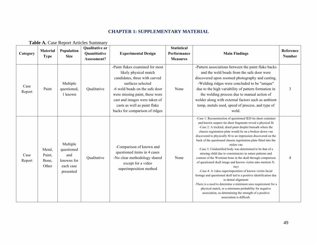
49
CHAPTER 1: SUPPLEMENTARY MATERIAL
Table A. Case Report Articles Summary
Category Material
Type
Population
Size
Qualitative or
Quantitative
Assessment?
Experimental Design
Statistical
Performance
Measures
Main Findings Reference
Number
Case
Report Paint
Multiple
questioned,
1 known
Qualitative
-Paint flakes examined for most
likely physical match
candidates, three with curved
surfaces selected
-6 weld beads on the safe door
were missing paint, these were
cast and images were taken of
casts as well as paint flake
backs for comparison of ridges
None
-Pattern associations between the paint flake backs
and the weld beads from the safe door were
discovered upon zoomed photography and casting.
-Welding ridges were concluded to be "unique"
due to the high variability of pattern formation in
the welding process due to manual action of
welder along with external factors such as ambient
temp, metals used, speed of process, and type of
weld.
3
Case
Report
Metal,
Paint,
Bone,
Other
Multiple
questioned
and
knowns for
each case
presented
Qualitative
-Comparison of known and
questioned items in 4 cases
-No clear methodology shared
except for a video
superimposition method
None
-Case 1: Reconstruction of questioned IED tin sheet container
and known suspect tin sheet fragments reveal a physical fit
-Case 2: A trickled, dried paint droplet beneath where the
chassis registration plate would lie on a broken-down van
discovered to physically fit to an impression discovered on the
back of the questioned chassis registration plate fitted into the
stolen van
-Case 3: Unidentified body was determined to be that of a
missing child due to consistencies in suture patterns and
contour of the Wormian bone in the skull through comparison
of questioned skull image and known victim ante-mortem X-
rays
-Case 4: A video-superimposition of known victim facial
footage and questioned skull led to a positive identification due
to dental alignment
-There is a need to determine a minimum area requirement for a
physical match, or a minimum probability for negative
association, as determining the strength of a positive
association is difficult.
4
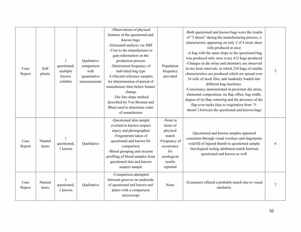
50
Case
Report
Soft
plastic
1
questioned,
multiple
known
exhibits
Qualitative
comparison
with
quantitative
measurements
-Observations of physical
features of the questioned and
known bags
-Elemental analysis via XRF
-Visit to the manufacturer to
gain information on the
production process
-Determined frequency of
individual bag type
-Collected reference samples
for determination of period of
manufacture time before feature
change
-Die line slope method
described by Von Bremen and
Blunt used to determine order
of manufacture
Population
frequency
provided
-Both questioned and known bags were the results
of “J sheets” during the manufacturing process, a
characteristic appearing on only 2 of 4 stock sheet
rolls produced at once
-A bag with the same slope as the questioned bag
was produced only once every 412 bags produced
-Changes in die striae and chemistry are observed
in two hour intervals, in which 254 bags of similar
characteristics are produced which are spread over
16 rolls of stock film, and randomly loaded into
different bag machines.
-Consistency demonstrated in persistent die striae,
elemental composition, tie flap offset, bag width,
degree of tie-flap centering and the presence of die
flap over-tucks (due to origination from “J-
sheets”) between the questioned and known bags
5
Case
Report
Natural
items
1
questioned,
1 known
Qualitative
-Questioned skin sample
overlaid to known suspect
injury and photographed
-Fingerprints taken of
questioned and known for
comparison
-Blood grouping and enzyme
profiling of blood samples from
questioned skin and known
suspect sample
-None in
terms of
physical
match
-Frequency of
occurrence
for
serological
results
reported
-Questioned and known samples appeared
consistent through visual overlays and fingerprint
void/fill of injured thumb to questioned sample
-Serological testing attributed match between
questioned and known as well
6
Case
Report
Natural
items
1
questioned,
1 known
Qualitative
-Comparison attempted
between grooves on underside
of questioned and known nail
plates with a comparison
microscope
None -Examiners offered a probable match due to visual
similarity 7
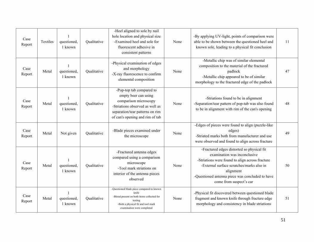
51
Case
Report Textiles
1
questioned,
1 known
Qualitative
-Heel aligned to sole by nail
hole location and physical size
-Examined heel and sole for
fluorescent adhesive in
consistent patterns
None
-By applying UV-light, points of comparison were
able to be shown between the questioned heel and
known sole, leading to a physical fit conclusion
11
Case
Report Metal
1
questioned,
1 known
Qualitative
-Physical examination of edges
and morphology
-X-ray fluorescence to confirm
elemental composition
None
-Metallic chip was of similar elemental
composition to the material of the fractured
padlock
-Metallic chip appeared to be of similar
morphology to the fractured edge of the padlock
47
Case
Report Metal
1
questioned,
1 known
Qualitative
-Pop-top tab compared to
empty beer can using
comparison microscopy
-Striations observed as well as
separation/tear patterns on rim
of can's opening and rim of tab
None
-Striations found to be in alignment
-Separation/tear pattern of pop-tab was also found
to be in alignment with rim of the can's opening
48
Case
Report Metal Not given Qualitative
-Blade pieces examined under
the microscope None
-Edges of pieces were found to align (puzzle-like
edges)
-Striated marks both from manufacturer and use
were observed and found to align across fracture
49
Case
Report Metal
1
questioned,
1 known
Qualitative
-Fractured antenna edges
compared using a comparison
microscope
-Tool mark striations on
interior of the antenna pieces
observed
None
-Fractured edges distorted so physical fit
examination was inconclusive
-Striations were found to align across fracture
-External surface scratches/marks also in
alignment
-Questioned antenna piece was concluded to have
come from suspect’s car
50
Case
Report Metal
1
questioned,
1 known
Qualitative
-Questioned blade piece compared to known
knife
-Blood present on both items collected for
testing
-Both a physical fit and tool mark
examination were completed
None
-Physical fit discovered between questioned blade
fragment and known knife through fracture edge
morphology and consistency in blade striations
51
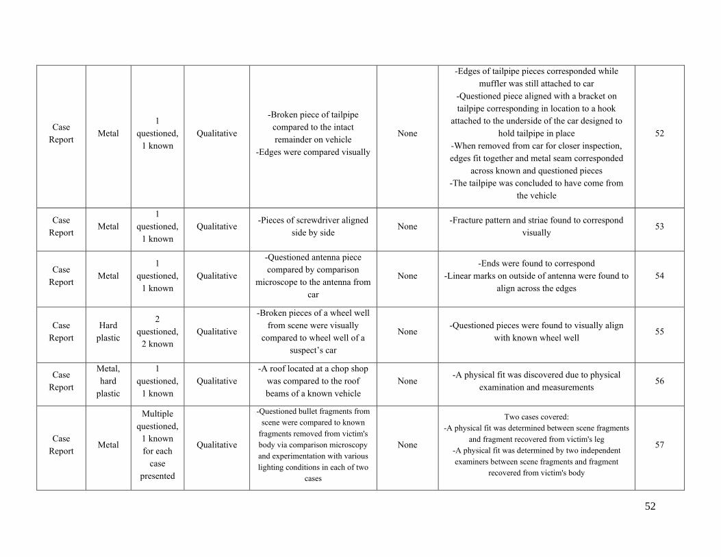
52
Case
Report Metal
1
questioned,
1 known
Qualitative
-Broken piece of tailpipe
compared to the intact
remainder on vehicle
-Edges were compared visually
None
-Edges of tailpipe pieces corresponded while
muffler was still attached to car
-Questioned piece aligned with a bracket on
tailpipe corresponding in location to a hook
attached to the underside of the car designed to
hold tailpipe in place
-When removed from car for closer inspection,
edges fit together and metal seam corresponded
across known and questioned pieces
-The tailpipe was concluded to have come from
the vehicle
52
Case
Report Metal
1
questioned,
1 known
Qualitative -Pieces of screwdriver aligned
side by side None
-Fracture pattern and striae found to correspond
visually 53
Case
Report Metal
1
questioned,
1 known
Qualitative
-Questioned antenna piece
compared by comparison
microscope to the antenna from
car
None
-Ends were found to correspond
-Linear marks on outside of antenna were found to
align across the edges
54
Case
Report
Hard
plastic
2
questioned,
2 known
Qualitative
-Broken pieces of a wheel well
from scene were visually
compared to wheel well of a
suspect’s car
None -Questioned pieces were found to visually align
with known wheel well 55
Case
Report
Metal,
hard
plastic
1
questioned,
1 known
Qualitative
-A roof located at a chop shop
was compared to the roof
beams of a known vehicle
None -A physical fit was discovered due to physical
examination and measurements 56
Case
Report Metal
Multiple
questioned,
1 known
for each
case
presented
Qualitative
-Questioned bullet fragments from
scene were compared to known
fragments removed from victim's
body via comparison microscopy
and experimentation with various
lighting conditions in each of two
cases
None
Two cases covered:
-A physical fit was determined between scene fragments
and fragment recovered from victim's leg
-A physical fit was determined by two independent
examiners between scene fragments and fragment
recovered from victim's body
57
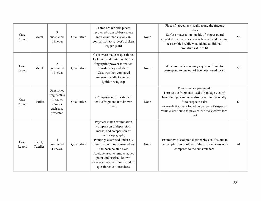
53
Case
Report Metal
3
questioned,
1 known
Qualitative
-Three broken rifle pieces
recovered from robbery scene
were examined visually in
comparison to suspect's broken
trigger guard
None
-Pieces fit together visually along the fracture
edges
-Surface material on outside of trigger guard
indicated that the stock was refinished and the gun
reassembled while wet, adding additional
probative value to fit
58
Case
Report Metal
2
questioned,
1 known
Qualitative
-Casts were made of questioned
lock core and dusted with grey
fingerprint powder to reduce
translucency and glare
-Cast was then compared
microscopically to known
ignition wing cap
None -Fracture marks on wing cap were found to
correspond to one out of two questioned locks 59
Case
Report Textiles
Questioned
fragment(s)
, 1 known
item for
each case
presented
Qualitative
-Comparison of questioned
textile fragment(s) to known
item
None
Two cases are presented:
-Torn textile fragments used to bandage victim's
hand during crime were discovered to physically
fit to suspect's shirt
-A textile fragment found on bumper of suspect's
vehicle was found to physically fit to victim's torn
coat
60
Case
Report
Paint,
Textiles
4
questioned,
4 known
Qualitative
-Physical match examination,
comparison of depression
marks, and comparison of
micro-topography
-Paintings examined under UV
illumination to recognize edges
had been painted over
-Acetone used to remove added
paint and original, known
canvas edges were compared to
questioned cut stretchers
None
-Examiners discovered distinct physical fits due to
the complex morphology of the distorted canvas as
compared to the cut stretchers
61
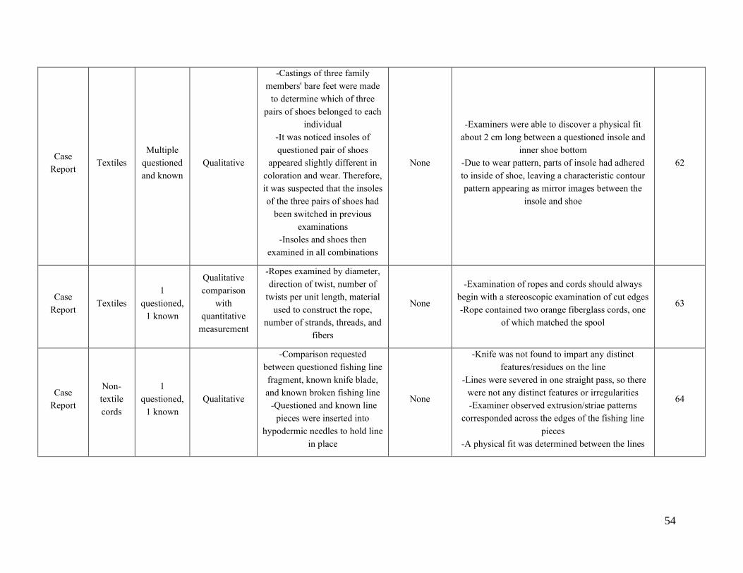
54
Case
Report Textiles
Multiple
questioned
and known
Qualitative
-Castings of three family
members' bare feet were made
to determine which of three
pairs of shoes belonged to each
individual
-It was noticed insoles of
questioned pair of shoes
appeared slightly different in
coloration and wear. Therefore,
it was suspected that the insoles
of the three pairs of shoes had
been switched in previous
examinations
-Insoles and shoes then
examined in all combinations
None
-Examiners were able to discover a physical fit
about 2 cm long between a questioned insole and
inner shoe bottom
-Due to wear pattern, parts of insole had adhered
to inside of shoe, leaving a characteristic contour
pattern appearing as mirror images between the
insole and shoe
62
Case
Report Textiles
1
questioned,
1 known
Qualitative
comparison
with
quantitative
measurement
-Ropes examined by diameter,
direction of twist, number of
twists per unit length, material
used to construct the rope,
number of strands, threads, and
fibers
None
-Examination of ropes and cords should always
begin with a stereoscopic examination of cut edges
-Rope contained two orange fiberglass cords, one
of which matched the spool
63
Case
Report
Non-
textile
cords
1
questioned,
1 known
Qualitative
-Comparison requested
between questioned fishing line
fragment, known knife blade,
and known broken fishing line
-Questioned and known line
pieces were inserted into
hypodermic needles to hold line
in place
None
-Knife was not found to impart any distinct
features/residues on the line
-Lines were severed in one straight pass, so there
were not any distinct features or irregularities
-Examiner observed extrusion/striae patterns
corresponded across the edges of the fishing line
pieces
-A physical fit was determined between the lines
64
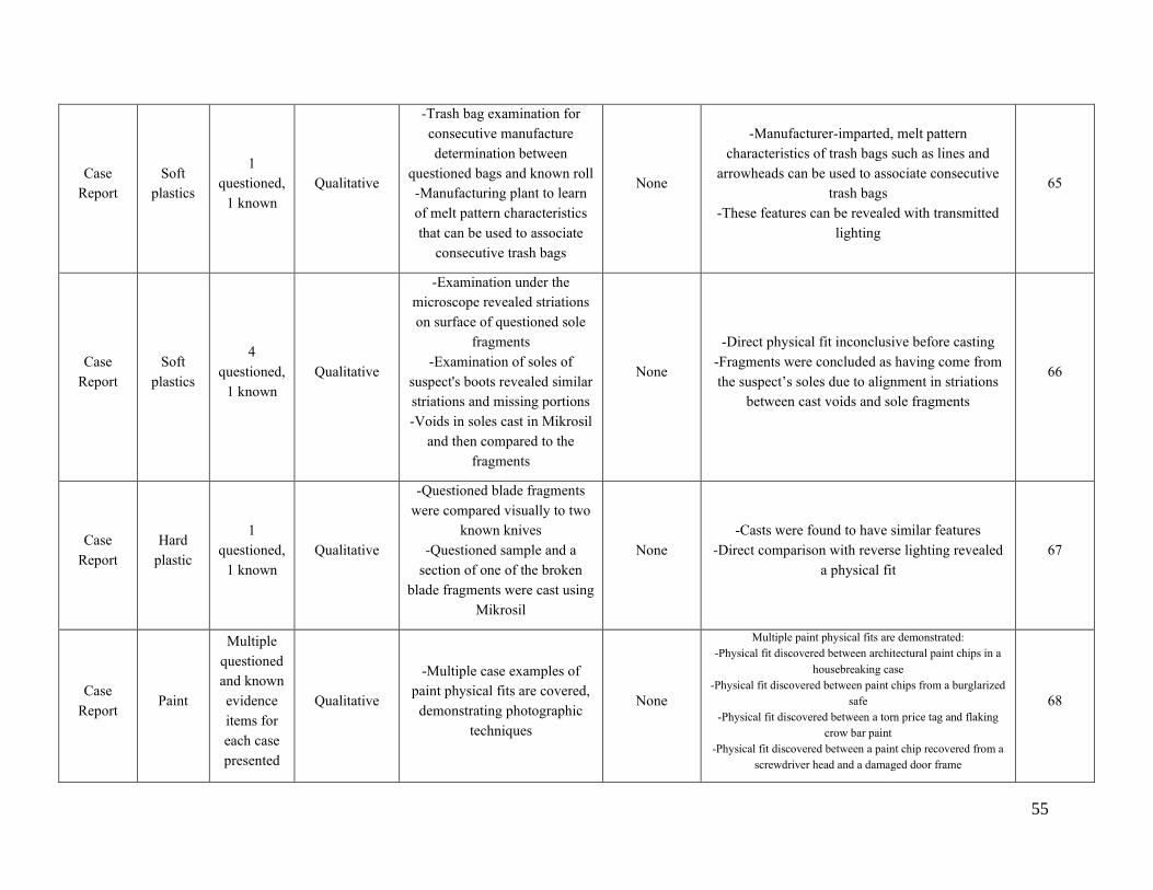
55
Case
Report
Soft
plastics
1
questioned,
1 known
Qualitative
-Trash bag examination for
consecutive manufacture
determination between
questioned bags and known roll
-Manufacturing plant to learn
of melt pattern characteristics
that can be used to associate
consecutive trash bags
None
-Manufacturer-imparted, melt pattern
characteristics of trash bags such as lines and
arrowheads can be used to associate consecutive
trash bags
-These features can be revealed with transmitted
lighting
65
Case
Report
Soft
plastics
4
questioned,
1 known
Qualitative
-Examination under the
microscope revealed striations
on surface of questioned sole
fragments
-Examination of soles of
suspect's boots revealed similar
striations and missing portions
-Voids in soles cast in Mikrosil
and then compared to the
fragments
None
-Direct physical fit inconclusive before casting
-Fragments were concluded as having come from
the suspect’s soles due to alignment in striations
between cast voids and sole fragments
66
Case
Report
Hard
plastic
1
questioned,
1 known
Qualitative
-Questioned blade fragments
were compared visually to two
known knives
-Questioned sample and a
section of one of the broken
blade fragments were cast using
Mikrosil
None
-Casts were found to have similar features
-Direct comparison with reverse lighting revealed
a physical fit
67
Case
Report Paint
Multiple
questioned
and known
evidence
items for
each case
presented
Qualitative
-Multiple case examples of
paint physical fits are covered,
demonstrating photographic
techniques
None
Multiple paint physical fits are demonstrated:
-Physical fit discovered between architectural paint chips in a
housebreaking case
-Physical fit discovered between paint chips from a burglarized
safe
-Physical fit discovered between a torn price tag and flaking
crow bar paint
-Physical fit discovered between a paint chip recovered from a
screwdriver head and a damaged door frame
68
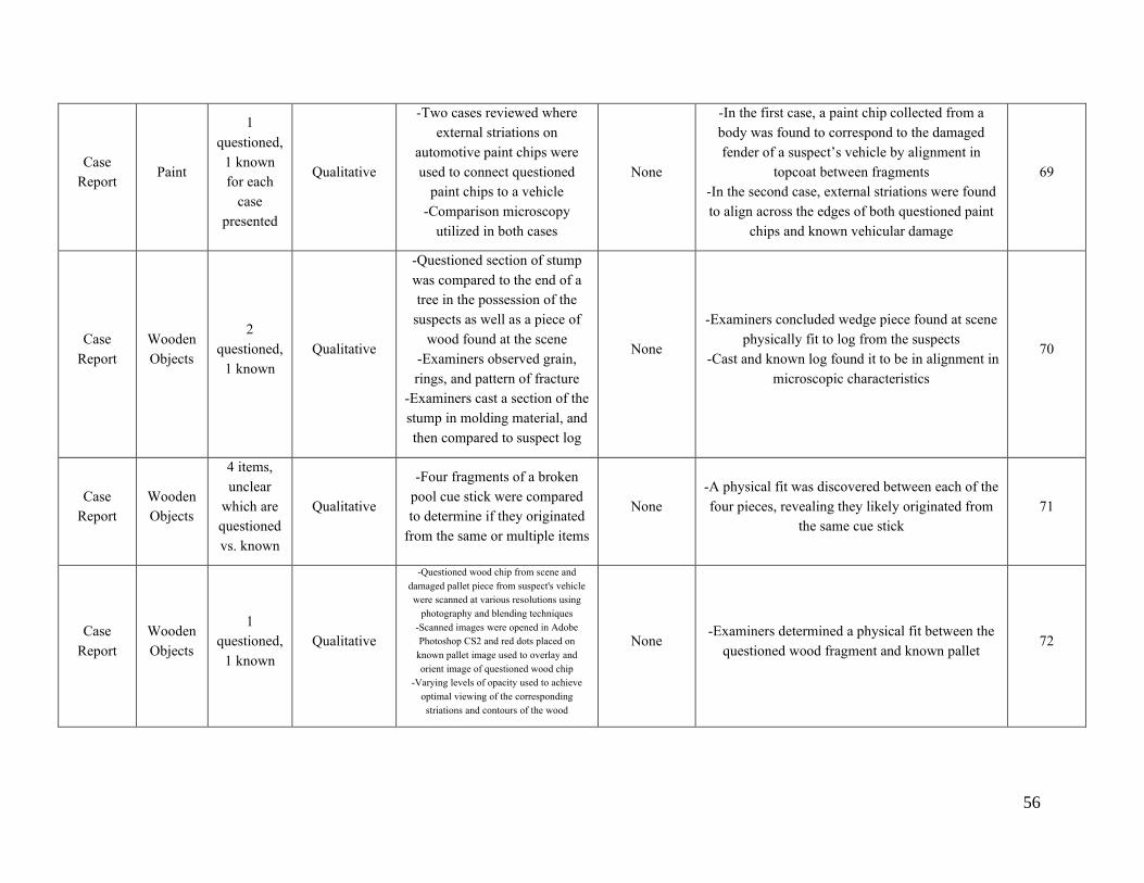
56
Case
Report Paint
1
questioned,
1 known
for each
case
presented
Qualitative
-Two cases reviewed where
external striations on
automotive paint chips were
used to connect questioned
paint chips to a vehicle
-Comparison microscopy
utilized in both cases
None
-In the first case, a paint chip collected from a
body was found to correspond to the damaged
fender of a suspect’s vehicle by alignment in
topcoat between fragments
-In the second case, external striations were found
to align across the edges of both questioned paint
chips and known vehicular damage
69
Case
Report
Wooden
Objects
2
questioned,
1 known
Qualitative
-Questioned section of stump
was compared to the end of a
tree in the possession of the
suspects as well as a piece of
wood found at the scene
-Examiners observed grain,
rings, and pattern of fracture
-Examiners cast a section of the
stump in molding material, and
then compared to suspect log
None
-Examiners concluded wedge piece found at scene
physically fit to log from the suspects
-Cast and known log found it to be in alignment in
microscopic characteristics
70
Case
Report
Wooden
Objects
4 items,
unclear
which are
questioned
vs. known
Qualitative
-Four fragments of a broken
pool cue stick were compared
to determine if they originated
from the same or multiple items
None
-A physical fit was discovered between each of the
four pieces, revealing they likely originated from
the same cue stick
71
Case
Report
Wooden
Objects
1
questioned,
1 known
Qualitative
-Questioned wood chip from scene and
damaged pallet piece from suspect's vehicle
were scanned at various resolutions using
photography and blending techniques
-Scanned images were opened in Adobe
Photoshop CS2 and red dots placed on
known pallet image used to overlay and
orient image of questioned wood chip
-Varying levels of opacity used to achieve
optimal viewing of the corresponding
striations and contours of the wood
None -Examiners determined a physical fit between the
questioned wood fragment and known pallet 72
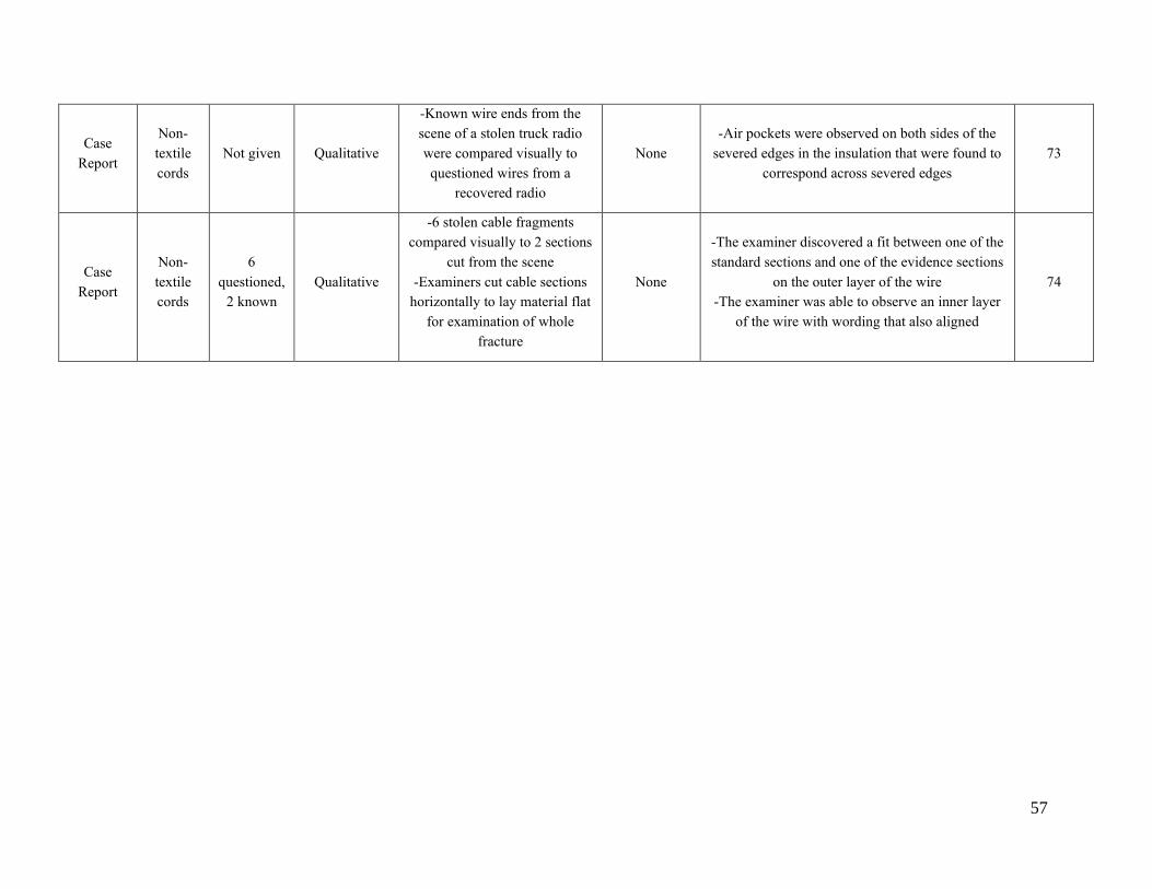
57
Case
Report
Non-
textile
cords
Not given Qualitative
-Known wire ends from the
scene of a stolen truck radio
were compared visually to
questioned wires from a
recovered radio
None
-Air pockets were observed on both sides of the
severed edges in the insulation that were found to
correspond across severed edges
73
Case
Report
Non-
textile
cords
6
questioned,
2 known
Qualitative
-6 stolen cable fragments
compared visually to 2 sections
cut from the scene
-Examiners cut cable sections
horizontally to lay material flat
for examination of whole
fracture
None
-The examiner discovered a fit between one of the
standard sections and one of the evidence sections
on the outer layer of the wire
-The examiner was able to observe an inner layer
of the wire with wording that also aligned
74
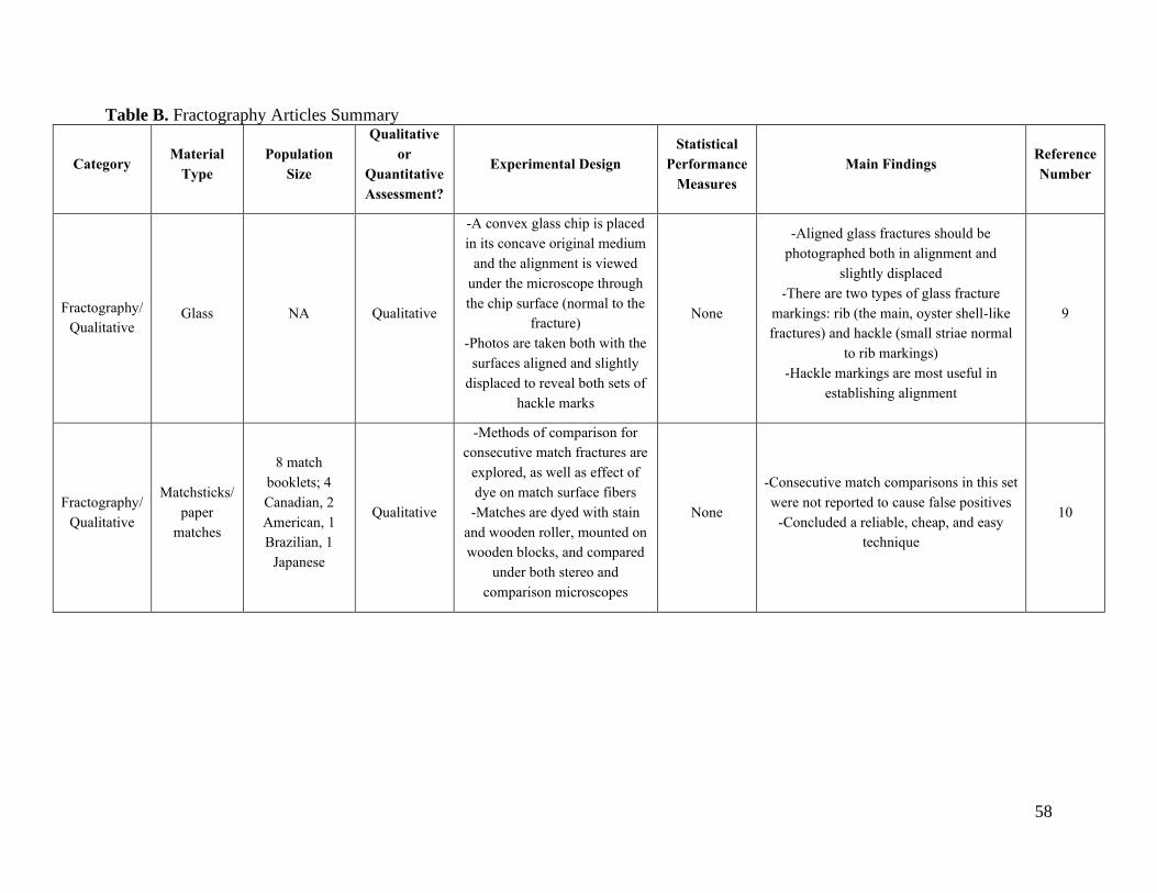
58
Table B. Fractography Articles Summary
Category Material
Type
Population
Size
Qualitative
or
Quantitative
Assessment?
Experimental Design
Statistical
Performance
Measures
Main Findings Reference
Number
Fractography/
Qualitative Glass NA Qualitative
-A convex glass chip is placed
in its concave original medium
and the alignment is viewed
under the microscope through
the chip surface (normal to the
fracture)
-Photos are taken both with the
surfaces aligned and slightly
displaced to reveal both sets of
hackle marks
None
-Aligned glass fractures should be
photographed both in alignment and
slightly displaced
-There are two types of glass fracture
markings: rib (the main, oyster shell-like
fractures) and hackle (small striae normal
to rib markings)
-Hackle markings are most useful in
establishing alignment
9
Fractography/
Qualitative
Matchsticks/
paper
matches
8 match
booklets; 4
Canadian, 2
American, 1
Brazilian, 1
Japanese
Qualitative
-Methods of comparison for
consecutive match fractures are
explored, as well as effect of
dye on match surface fibers
-Matches are dyed with stain
and wooden roller, mounted on
wooden blocks, and compared
under both stereo and
comparison microscopes
None
-Consecutive match comparisons in this set
were not reported to cause false positives
-Concluded a reliable, cheap, and easy
technique
10
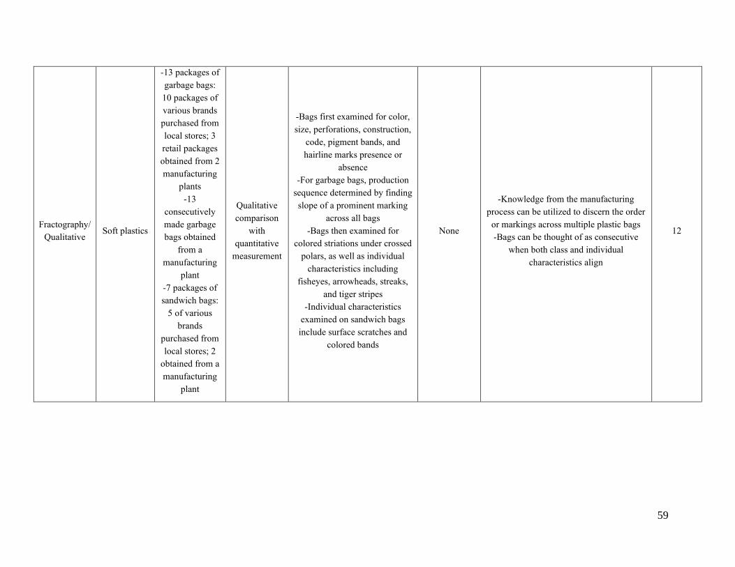
59
Fractography/
Qualitative Soft plastics
-13 packages of
garbage bags:
10 packages of
various brands
purchased from
local stores; 3
retail packages
obtained from 2
manufacturing
plants
-13
consecutively
made garbage
bags obtained
from a
manufacturing
plant
-7 packages of
sandwich bags:
5 of various
brands
purchased from
local stores; 2
obtained from a
manufacturing
plant
Qualitative
comparison
with
quantitative
measurement
-Bags first examined for color,
size, perforations, construction,
code, pigment bands, and
hairline marks presence or
absence
-For garbage bags, production
sequence determined by finding
slope of a prominent marking
across all bags
-Bags then examined for
colored striations under crossed
polars, as well as individual
characteristics including
fisheyes, arrowheads, streaks,
and tiger stripes
-Individual characteristics
examined on sandwich bags
include surface scratches and
colored bands
None
-Knowledge from the manufacturing
process can be utilized to discern the order
or markings across multiple plastic bags
-Bags can be thought of as consecutive
when both class and individual
characteristics align
12
60
Fractography/
Qualitative Paints
6 vehicles, 2
models (Ford
Telstar and
Ford Laser),
two points of
contact in hinge
of driver's door
per vehicle
Qualitative
-Two points of contact were
photographed in driver door
hinge area of 6 vehicles at a
production plant
-Photographs, as well as their
negatives, were compared over
a light box for pattern
consistency between known
door and hinge, and also
between vehicles
None
-Gaps between panels allowed capillaries
of the surface coating to form, revealing
striations that could be aligned between
door and hinge
-Corresponding pattern would appear on a
panel beside door if capillaries broke
unevenly
-If there was poor electro coating between
panels, these patterns would not be
displayed at all
-Patterns were distinguishable between
vehicles
-Methods of court presentation: mounting
photographs to reveal the mirror image,
reversing one of the images to directly
show points of comparison, or producing a
high contrast transparency of one of the
photographs to be overlaid on the other
14
Fractography/
Qualitative
Glass,
Metal, Hard
plastics
Not given Qualitative
-Three different loads were used
(0.98N, 2.0N, and 2.9N) for a hard
indenter to reproducibly create
fractures
-The second part of the study was
bending of glass, in which a
universal testing machine was used
to create reproducible load
distributions
-The third test was with polymers
using an impact “hail-stone gun”.
Plastic balls were discharged at
polymethyl methacrylate (PMMA)
sheets
-Tensile tests completed on steel
wires
None
-Fractures were found to have random
distributions of cracks
-Cracks themselves were found to have
random number, lengths, propagations,
directions, shapes, and orientations
-Curves and fractures made in the second
study were also randomly distributed
-Cracks from the impact (third study) was
found to also be random
-Curves and fracture surfaces of the wires
were random and varied between the
different wires, despite being made of the
same material
-The steel wires were found to allow for a
fracture match between the edges
77
61
Fractography/
Qualitative Tape Not given Qualitative
-Tapes from six different
manufacturers were torn by
hand and observed with a
comparison microscope
-The edges treated with 100
Celsius hot air for a few
seconds
-After treatment the tapes were
re-observed under comparison
microscopy
None
-Heat treatment was found to make it
easier to find the corresponding edge, and
improved confidence in the conclusion
-The author did note however that
applying heat treatment may destroy other
evidence (DNA, fingerprints)
78
Fractography/
Qualitative Tape NA Qualitative
-Tapes were either sheared or
torn, heat-treated at 100°C with
demineralized water to undo
any plastic deformation
occurring after fracture, cast
with casting material, and each
edge of the fracture cast was
examined using comparison
microscopy for fracture
matching
None
-Each tested fracture generated an
individual fracture pattern of which a cast
could be taken for nearly mirror-image
comparison microscopy results
79
Fractography/
Qualitative Tape Not given Qualitative
-Tapes torn by hand and cut
with scissors to demonstrate
non-reproducibility
None
-Tearing and shearing black electrical tape
samples left distinct tears that were non-
reproducible
80
Fractography/
Qualitative Soft plastics NA Qualitative
-A review/recommendation for analysis
of garbage bags for consecutive
manufacturing identification rather than
a study with actual samples
-Garbage bags can be aligned according
to their heat-sealed edges/ending.
Transmitted light from underneath can
reveal striations from the
manufacturing process that can attribute
to a common source
None
-Horizontal streaks in plastic bag material
formed during the manufacturing process are in
the following categories:
1-fisheyes (randomly-distributed dark
pigments)
2-arrowheads (triangular striae of dark pigment)
3-tiger stripes (horizontal striae of dark
pigment)
4-die lines (become visible in the blowing and
stretching process, straight horizontal lines)
81
62
Fractography/
Qualitative Soft plastics NA Qualitative
-Summary of characteristics of
polyethylene films that can be
used for comparisons and
manufacturing processes
NA
-Additives to films from manufacturing
appear as striations/patterning
-Extrusion marks originate from the roller
-Additional scratches and surface striations
come from machine wear
-Dye variations come from uneven
applications of dye
82
Fractography/
Qualitative Soft plastics NA Qualitative
-Black card was cut to have ⅛
in X 6 ½ slots. Two sheets of
glass were put together and
placed above the grid. The grid
was illuminated by a 500-watt
lamp at a right angle
-Camera was focused on the
glass in the frame so that the
whole area of glass would be in
the negative
-Polyethylene piece was
sandwiched between the glass
sheets with the extrusion marks
on the short side
NA
-The photography method was found to be
useful for visualizing and documenting
extrusion marks in polyethylene film
83
63
Fractography/
Qualitative Soft plastics NA Qualitative
-This paper focuses on
photographing physical
characteristics of plastic bags
and film that have potential to
be used to denote matching
edges or connected pieces of
evidence
None
-Extrusion marks are recommended to be
photographed using a secondary lens
system so that the extrusion marks can be
focused at any magnification
-Heat marks originate from bags that are
sealed together by an individual separately
from the manufacturing heat seals
-Secondary heat marks were often created
using a soldering iron or laundry iron, or
by commercially made sealing machines
-For sealing machines, conclusions could
be made by examining the patterns left by
the heat proof fabric on the machine, by
observing inclusions and irregularities
created in consecutive seals made by the
same machine, and by hot spots (unique
areas of deformation caused by heat)
-Cut edges of films could offer some
additional details if the instrument used to
sever the edges left similar characteristics
(snags, changes in direction of cut, etc.)
84
64
Fractography/
Qualitative Soft plastics NA Qualitative
-Summary of a variety of
methods that can be used to
visualize and assess physical
properties of plastic bags and
cling film
-Kinds of properties that can be
utilized include color and
variation of die lines,
polarization patterns, striations
from manufacturing
-Summary as well of the
manufacturing of plastic bags
and film:
-Manufacturing: plastic bags
are made by blowing polymer
through a circular tube and then
flattened. Cling film is also
made by a blown film
extrusion, but forms a single
sheet that is wound up
-Finally, four cases mentioned
in which characteristics of
plastic bags were viewed to
allow for matching
None
-Polarization (polarization table): used
because many polymeric films are
birefringent. Consecutively produced bags
often have similar or consecutive colors
under cross-polars, and the patterns can be
compared to fit matching bags together
-Shadowgraph and Schlieren imaging:
shadowgraphs involve a point light source
at an angle to the film, highlighting
discontinuities and defects within the film.
The film is photographed in front of the
light. For Schlieren, point source is
directed through a convex lens or spherical
mirror so that a parallel beam of light
passes through the film. A matching lens
or mirror catches the light and allows for
photography
-Incident and transmitted light microscopy:
microscopes that can be adjusted to allow
for visualization of inhomogeneities of the
films
-Four cases include an instance of printing
defects showing bags produced on the
same production line, a case where the
polarizations colors demonstrated the bags
were produced consecutively, a case where
the polarization, die lines, and striations
demonstrated consecutive manufacturing,
and finally a case where cling film die
lines demonstrated consecutive
manufacturing
85
65
Fractography/
Qualitative Glass NA Qualitative
-Multiple experiments
described without much
information on methodology
-Looking at how glass fractures
rather than how to piece broken
glass back together
None
-Two major types of fractures: radial and
concentric
-Arcs on radial fractures present concave
opposite the origin of the breaking force,
while the opposite is true of concentric
-Only occurrences of first-order fracture
surfaces (fracture center and first
concentric fracture) should be considered
reliable
-Bullet holes in safety glass have different
chipping - the entrance pane will have
perpendicular chips, the exit will have
chips at an angle with the surface
86
Fractography/
Qualitative Glass
16 glass
samples (4
types)
Quantitative
-Window panes at three
different thicknesses were shot
with a 4.5 mm air rifle
-Various measurements
recorded on the fracture
patterns including radial
fracture count, concentric
fracture count, bullet hole
diameter, mist zone thickness,
and mist zone diameter
-Chi-Square
Test used to
assess
goodness of
fit or minimal
variation for
measurement
trend lines
-No significant differences were present in
fracture pattern measurements between
both all glass thicknesses, regardless of sun
control film
-Bullet hole diameters in regular rifles tend
to be double the caliber of the firearm
while those of air rifles tend to be similar
to the weapon's caliber. This may be useful
in distinguishing between weapon type
87
66
Fractography/
Qualitative Glass NA Qualitative
-Quasi-static loading can result
in glass fractures with no
obvious distortions in the glass
-Fracture occurs when the glass
fails at a Griffith crack (minute
flaws that are often a point of
stress concentration)
None
-Dynamic loading is discussed, including
how kinetic energy is transferred to glass -
mainly through direct force by the
projectile and mechanical waves
-The waves produce stress on the glass
structure as the waves reflect off the back
and front of the glass
-The high stress impact of the mechanical
waves creates a crater in the glass,
although penetration of the glass is not
necessary for crater formation as long as
there is enough stress applied to a weak
point/flaw
-Though high amounts of energy may be
transferred, if the velocity of the crack
propagation is not propagated for long, the
extent of the fracturing may be minimal
around the crater
-While cratering can be useful in
reconstruction if the calibers are known,
the size and distribution of the crater and
resulting fractures cannot be used to
provide definitive information about the
calibers if unknown
88
67
Fractography/
Qualitative
Glass, hard
plastic
60 panes
double-strength
glass, 60 clear
glass wine
bottles, 60
polymer
taillight lenses
Qualitative
-60 each of three sample types,
two fracture methods: dynamic
impact and static pressure, 30
samples each, three fracture tips
(blunt, round, sharp)
-Dynamic: 8x8” glass panes,
wine bottles coated with RTV
urethane, 5.5/8x4.1/4” plastic
lens, 10 glass samples per
dropping weight impact tip, 10
plastic lenses per dropping
height, reassembled, imaged,
and videoed for velocity
measurements
-Static: 8x8” sample, wine
bottles coated with RTV
urethane, indenter crosshead
speed 10 mm/min, 10 samples
per indenter tip (only wide tip
used on plastic so all 30 were
the same), load vs extension
measured by Instron software,
reassembled and imaged
-Visual comparisons: fractures
traced onto acetate and overlay
one-to-one per sample at four
orientations (two for bottles)
None
-Blunt fracture tip required the highest
velocity (dynamic) and force (static) while
sharp tips required the least
-Sharp tip fracture patterns contained
fewest lines, blunt tip pattern contained
most lines
Glass panes: Blunt tip created more radial
and concentric fractures, and dynamic
fracture patterns more simple than static
Wine bottles: Number of fractures
between impact tips more evenly
distributed, and fracture patterns between
dynamic and static samples did not vary as
much
-Linear relationship expected between
load and extension, curvature obtained
from load profiles
-In plastic lenses, velocity increased as
drop height increased, causing a center
crushing and edge fracturing
-Plastic extension value exceeds glass
values, however load is smaller
89,90
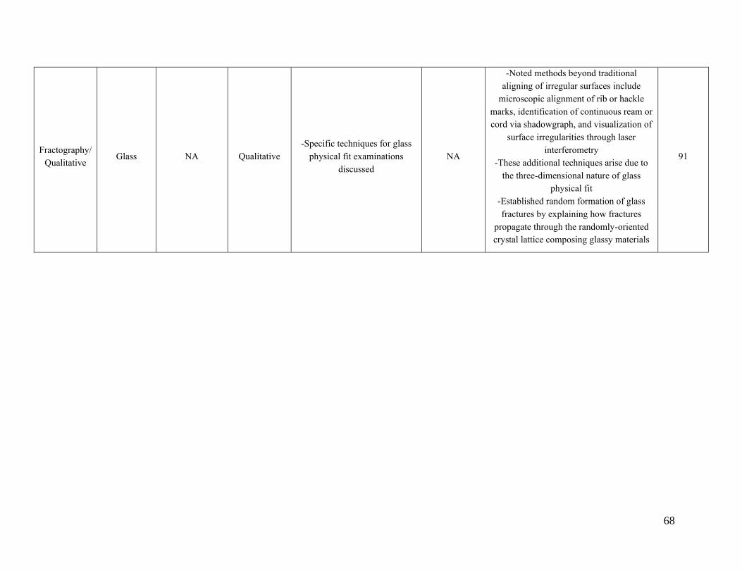
68
Fractography/
Qualitative Glass NA Qualitative
-Specific techniques for glass
physical fit examinations
discussed
NA
-Noted methods beyond traditional
aligning of irregular surfaces include
microscopic alignment of rib or hackle
marks, identification of continuous ream or
cord via shadowgraph, and visualization of
surface irregularities through laser
interferometry
-These additional techniques arise due to
the three-dimensional nature of glass
physical fit
-Established random formation of glass
fractures by explaining how fractures
propagate through the randomly-oriented
crystal lattice composing glassy materials
91
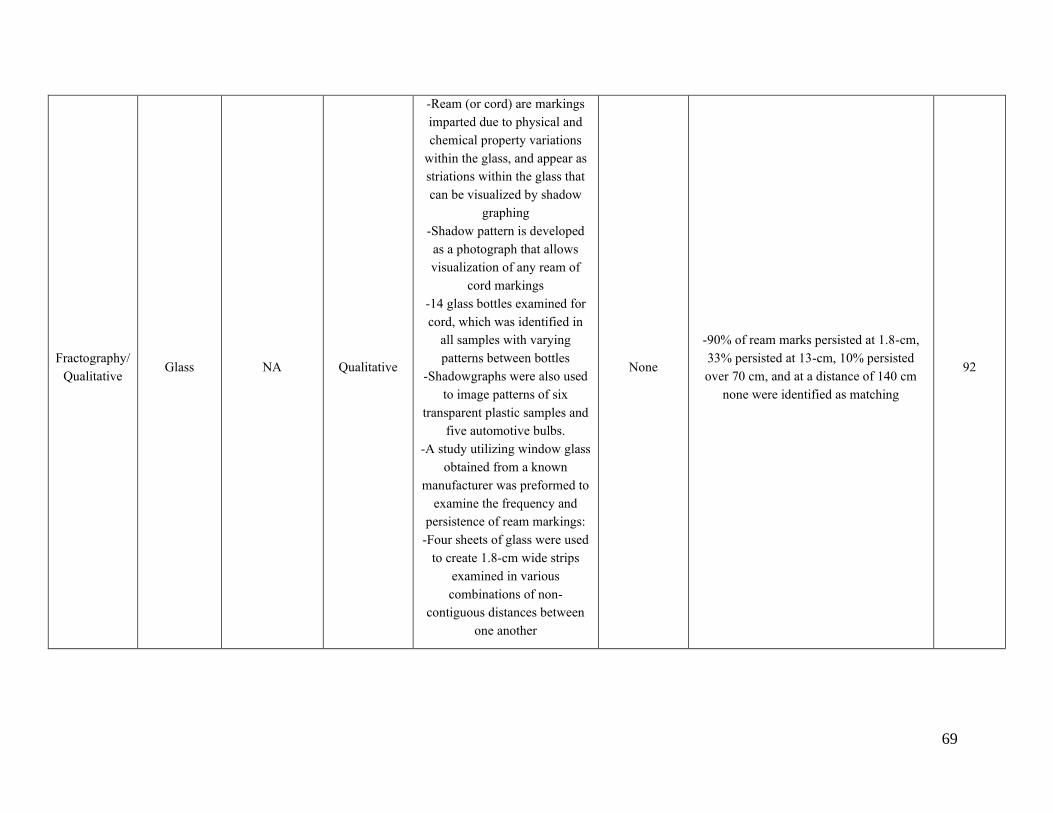
69
Fractography/
Qualitative Glass NA Qualitative
-Ream (or cord) are markings
imparted due to physical and
chemical property variations
within the glass, and appear as
striations within the glass that
can be visualized by shadow
graphing
-Shadow pattern is developed
as a photograph that allows
visualization of any ream of
cord markings
-14 glass bottles examined for
cord, which was identified in
all samples with varying
patterns between bottles
-Shadowgraphs were also used
to image patterns of six
transparent plastic samples and
five automotive bulbs.
-A study utilizing window glass
obtained from a known
manufacturer was preformed to
examine the frequency and
persistence of ream markings:
-Four sheets of glass were used
to create 1.8-cm wide strips
examined in various
combinations of non-
contiguous distances between
one another
None
-90% of ream marks persisted at 1.8-cm,
33% persisted at 13-cm, 10% persisted
over 70 cm, and at a distance of 140 cm
none were identified as matching
92
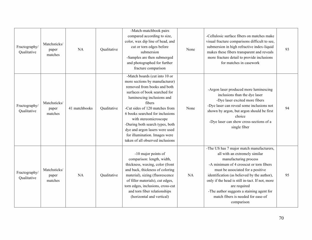
70
Fractography/
Qualitative
Matchsticks/
paper
matches
NA Qualitative
-Match-matchbook pairs
compared according to size,
color, wax dip line of head, and
cut or torn edges before
submersion
-Samples are then submerged
and photographed for further
fracture comparison
None
-Cellulosic surface fibers on matches make
visual fracture comparisons difficult to see,
submersion in high refractive index-liquid
makes these fibers transparent and reveals
more fracture detail to provide inclusions
for matches in casework
93
Fractography/
Qualitative
Matchsticks/
paper
matches
41 matchbooks Qualitative
-Match boards (cut into 10 or
more sections by manufacturer)
removed from books and both
surfaces of book searched for
luminescing inclusions and
fibers
-Cut sides of 120 matches from
6 books searched for inclusions
with stereomicroscope
-During both search types, both
dye and argon lasers were used
for illumination. Images were
taken of all observed inclusions
None
-Argon laser produced more luminescing
inclusions than the dye laser
-Dye laser excited more fibers
-Dye laser can reveal some inclusions not
shown by argon, but argon should be first
choice
-Dye laser can show cross-sections of a
single fiber
94
Fractography/
Qualitative
Matchsticks/
paper
matches
NA Qualitative
-10 major points of
comparison: length, width,
thickness, waxing, color (front
and back, thickness of coloring
material), sizing (fluorescence
of filler materials), cut edges,
torn edges, inclusions, cross-cut
and torn fiber relationships
(horizontal and vertical)
NA
-The US has 7 major match manufacturers,
all with an extremely similar
manufacturing process
-A minimum of 4 crosscut or torn fibers
must be associated for a positive
identification (as believed by the author),
only if the head is still in-tact. If not, more
are required
-The author suggests a staining agent for
match fibers is needed for ease-of
comparison
95
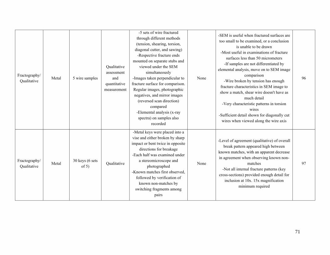
71
Fractography/
Qualitative Metal 5 wire samples
Qualitative
assessment
and
quantitative
measurement
-5 sets of wire fractured
through different methods
(tension, shearing, torsion,
diagonal cutter, and sawing)
-Respective fracture ends
mounted on separate stubs and
viewed under the SEM
simultaneously
-Images taken perpendicular to
fracture surface for comparison.
Regular images, photographic
negatives, and mirror images
(reversed scan direction)
compared
-Elemental analysis (x-ray
spectra) on samples also
recorded
None
-SEM is useful when fractured surfaces are
too small to be examined, or a conclusion
is unable to be drawn
-Most useful in examinations of fracture
surfaces less than 50 micrometers
-If samples are not differentiated by
elemental analysis, move on to SEM image
comparison
-Wire broken by tension has enough
fracture characteristics in SEM image to
show a match, shear wire doesn't have as
much detail
-Very characteristic patterns in torsion
wires
-Sufficient detail shown for diagonally cut
wires when viewed along the wire axis
96
Fractography/
Qualitative Metal
30 keys (6 sets
of 5) Qualitative
-Metal keys were placed into a
vise and either broken by sharp
impact or bent twice in opposite
directions for breakage
-Each half was examined under
a stereomicroscope and
photographed
-Known matches first observed,
followed by verification of
known non-matches by
switching fragments among
pairs
None
-Level of agreement (qualitative) of overall
break pattern appeared high between
known matches, with an apparent decrease
in agreement when observing known non-
matches
-Not all internal fracture patterns (key
cross-sections) provided enough detail for
inclusion at 10x. 15x magnification
minimum required
97
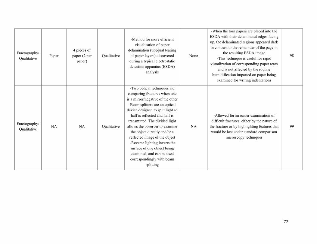
72
Fractography/
Qualitative Paper
4 pieces of
paper (2 per
paper)
Qualitative
-Method for more efficient
visualization of paper
delamination (unequal tearing
of paper layers) discovered
during a typical electrostatic
detection apparatus (ESDA)
analysis
None
-When the torn papers are placed into the
ESDA with their delaminated edges facing
up, the delaminated regions appeared dark
in contrast to the remainder of the page in
the resulting ESDA image
-This technique is useful for rapid
visualization of corresponding paper tears
and is not affected by the routine
humidification imparted on paper being
examined for writing indentations
98
Fractography/
Qualitative NA NA Qualitative
-Two optical techniques aid
comparing fractures when one
is a mirror/negative of the other
-Beam splitters are an optical
device designed to split light so
half is reflected and half is
transmitted. The divided light
allows the observer to examine
the object directly and/or a
reflected image of the object
-Reverse lighting inverts the
surface of one object being
examined, and can be used
correspondingly with beam
splitting
NA
-Allowed for an easier examination of
difficult fractures, either by the nature of
the fracture or by highlighting features that
would be lost under standard comparison
microscopy techniques
99
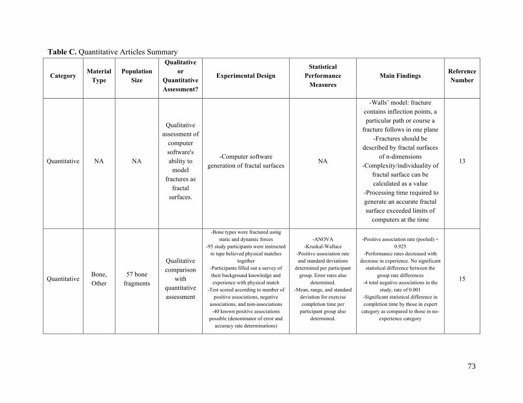
73
Table C. Quantitative Articles Summary
Category Material
Type
Population
Size
Qualitative
or
Quantitative
Assessment?
Experimental Design
Statistical
Performance
Measures
Main Findings Reference
Number
Quantitative NA NA
Qualitative
assessment of
computer
software's
ability to
model
fractures as
fractal
surfaces.
-Computer software
generation of fractal surfaces NA
-Walls’ model: fracture
contains inflection points, a
particular path or course a
fracture follows in one plane
-Fractures should be
described by fractal surfaces
of n-dimensions
-Complexity/individuality of
fractal surface can be
calculated as a value
-Processing time required to
generate an accurate fractal
surface exceeded limits of
computers at the time
13
Quantitative Bone,
Other
57 bone
fragments
Qualitative
comparison
with
quantitative
assessment
-Bone types were fractured using
static and dynamic forces
-95 study participants were instructed
to tape believed physical matches
together
-Participants filled out a survey of
their background knowledge and
experience with physical match
-Test scored according to number of
positive associations, negative
associations, and non-associations
-40 known positive associations
possible (denominator of error and
accuracy rate determinations)
-ANOVA
-Kruskal-Wallace
-Positive association rate
and standard deviations
determined per participant
group. Error rates also
determined.
-Mean, range, and standard
deviation for exercise
completion time per
participant group also
determined.
-Positive association rate (pooled) =
0.925
-Performance rates decreased with
decrease in experience. No significant
statistical difference between the
group rate differences
-4 total negative associations in the
study, rate of 0.001
-Significant statistical difference in
completion time by those in expert
category as compared to those in no-
experience category
15
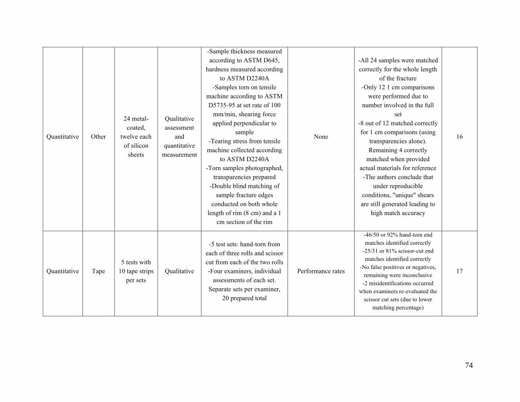
74
Quantitative Other
24 metal-
coated,
twelve each
of silicon
sheets
Qualitative
assessment
and
quantitative
measurement
-Sample thickness measured
according to ASTM D645,
hardness measured according
to ASTM D2240A
-Samples torn on tensile
machine according to ASTM
D5735-95 at set rate of 100
mm/min, shearing force
applied perpendicular to
sample
-Tearing stress from tensile
machine collected according
to ASTM D2240A
-Torn samples photographed,
transparencies prepared
-Double blind matching of
sample fracture edges
conducted on both whole
length of rim (8 cm) and a 1
cm section of the rim
None
-All 24 samples were matched
correctly for the whole length
of the fracture
-Only 12 1 cm comparisons
were performed due to
number involved in the full
set
-8 out of 12 matched correctly
for 1 cm comparisons (using
transparencies alone).
Remaining 4 correctly
matched when provided
actual materials for reference
-The authors conclude that
under reproducible
conditions, "unique" shears
are still generated leading to
high match accuracy
16
Quantitative Tape
5 tests with
10 tape strips
per sets
Qualitative
-5 test sets: hand-torn from
each of three rolls and scissor
cut from each of the two rolls
-Four examiners, individual
assessments of each set.
Separate sets per examiner,
20 prepared total
Performance rates
-46/50 or 92% hand-torn end
matches identified correctly
-25/31 or 81% scissor-cut end
matches identified correctly
-No false positives or negatives,
remaining were inconclusive
-2 misidentifications occurred
when examiners re-evaluated the
scissor cut sets (due to lower
matching percentage)
17
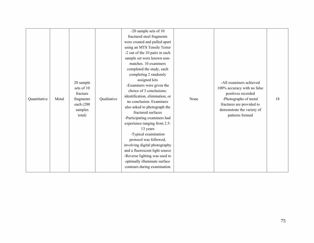
75
Quantitative Metal
20 sample
sets of 10
fracture
fragments
each (200
samples
total)
Qualitative
-20 sample sets of 10
fractured steel fragments
were created and pulled apart
using an MTS Tensile Tester
-2 out of the 10 pairs in each
sample set were known non-
matches. 10 examiners
completed the study, each
completing 2 randomly
assigned kits
-Examiners were given the
choice of 3 conclusions:
identification, elimination, or
no conclusion. Examiners
also asked to photograph the
fractured surfaces
-Participating examiners had
experience ranging from 2.5-
13 years
-Typical examination
protocol was followed,
involving digital photography
and a fluorescent light source
-Reverse lighting was used to
optimally illuminate surface
contours during examination
None
-All examiners achieved
100% accuracy with no false
positives recorded
-Photographs of metal
fractures are provided to
demonstrate the variety of
patterns formed
18
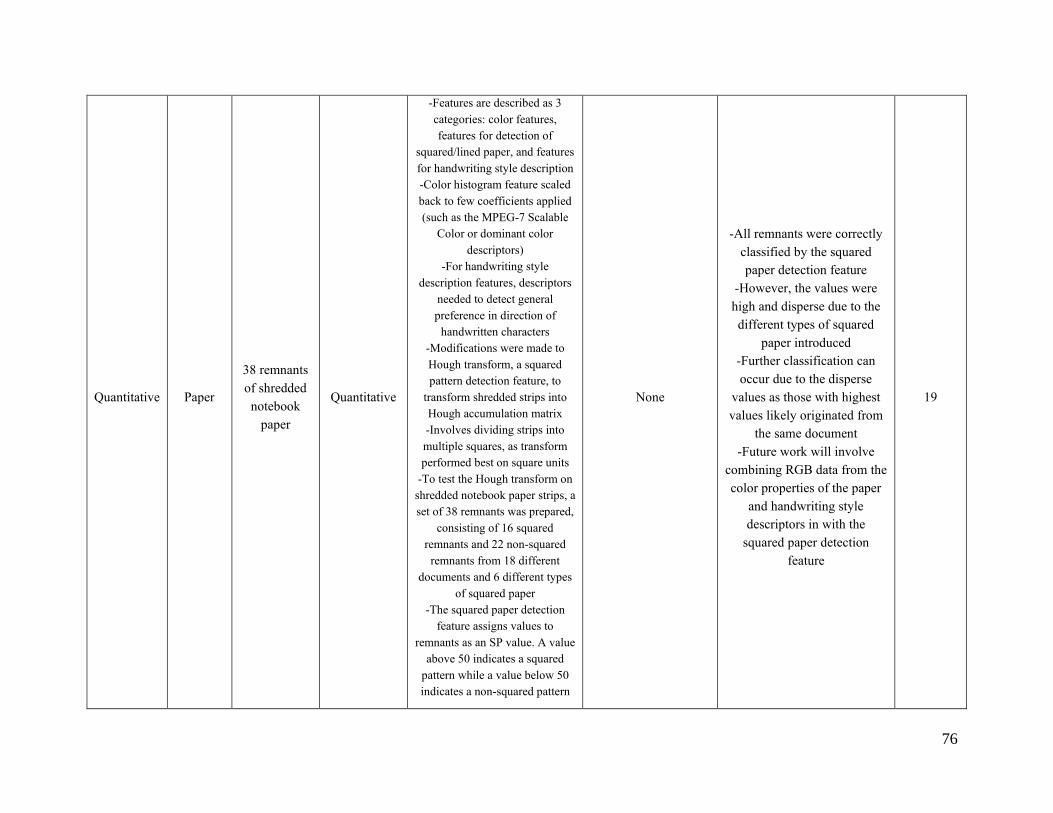
76
Quantitative Paper
38 remnants
of shredded
notebook
paper
Quantitative
-Features are described as 3
categories: color features,
features for detection of
squared/lined paper, and features
for handwriting style description
-Color histogram feature scaled
back to few coefficients applied
(such as the MPEG-7 Scalable
Color or dominant color
descriptors)
-For handwriting style
description features, descriptors
needed to detect general
preference in direction of
handwritten characters
-Modifications were made to
Hough transform, a squared
pattern detection feature, to
transform shredded strips into
Hough accumulation matrix
-Involves dividing strips into
multiple squares, as transform
performed best on square units
-To test the Hough transform on
shredded notebook paper strips, a
set of 38 remnants was prepared,
consisting of 16 squared
remnants and 22 non-squared
remnants from 18 different
documents and 6 different types
of squared paper
-The squared paper detection
feature assigns values to
remnants as an SP value. A value
above 50 indicates a squared
pattern while a value below 50
indicates a non-squared pattern
None
-All remnants were correctly
classified by the squared
paper detection feature
-However, the values were
high and disperse due to the
different types of squared
paper introduced
-Further classification can
occur due to the disperse
values as those with highest
values likely originated from
the same document
-Future work will involve
combining RGB data from the
color properties of the paper
and handwriting style
descriptors in with the
squared paper detection
feature
19
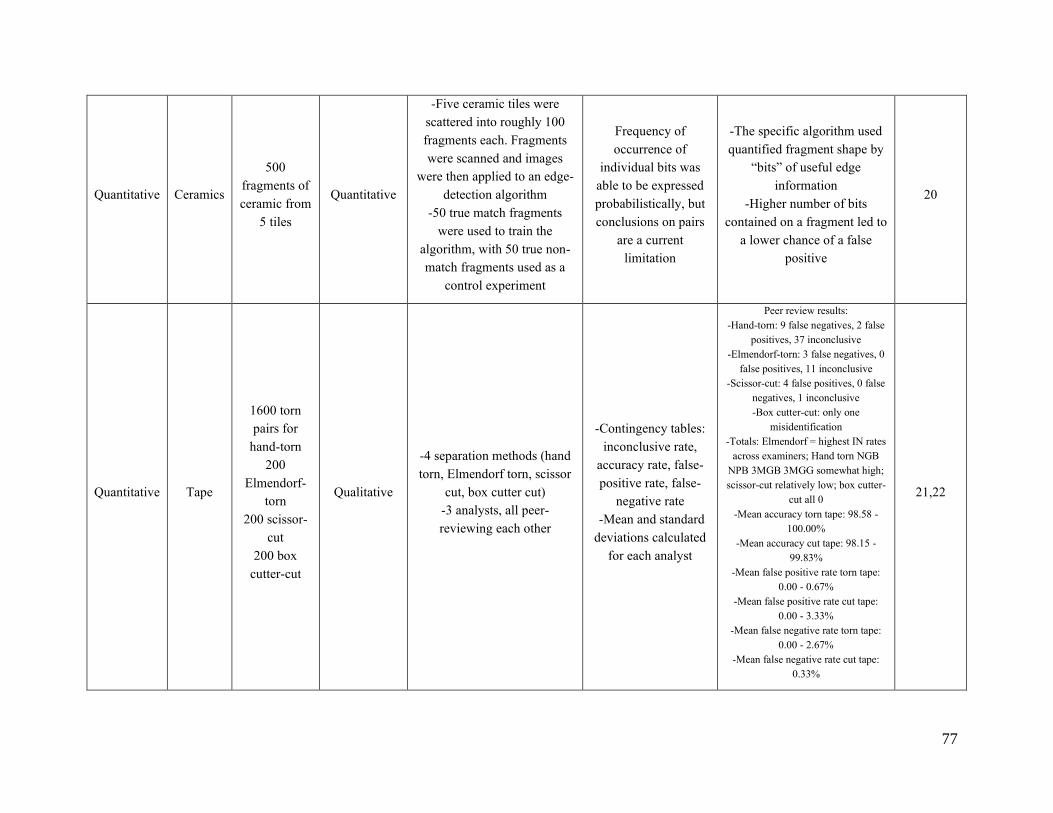
77
Quantitative Ceramics
500
fragments of
ceramic from
5 tiles
Quantitative
-Five ceramic tiles were
scattered into roughly 100
fragments each. Fragments
were scanned and images
were then applied to an edge-
detection algorithm
-50 true match fragments
were used to train the
algorithm, with 50 true non-
match fragments used as a
control experiment
Frequency of
occurrence of
individual bits was
able to be expressed
probabilistically, but
conclusions on pairs
are a current
limitation
-The specific algorithm used
quantified fragment shape by
“bits” of useful edge
information
-Higher number of bits
contained on a fragment led to
a lower chance of a false
positive
20
Quantitative Tape
1600 torn
pairs for
hand-torn
200
Elmendorf-
torn
200 scissor-
cut
200 box
cutter-cut
Qualitative
-4 separation methods (hand
torn, Elmendorf torn, scissor
cut, box cutter cut)
-3 analysts, all peer-
reviewing each other
-Contingency tables:
inconclusive rate,
accuracy rate, false-
positive rate, false-
negative rate
-Mean and standard
deviations calculated
for each analyst
Peer review results:
-Hand-torn: 9 false negatives, 2 false
positives, 37 inconclusive
-Elmendorf-torn: 3 false negatives, 0
false positives, 11 inconclusive
-Scissor-cut: 4 false positives, 0 false
negatives, 1 inconclusive
-Box cutter-cut: only one
misidentification
-Totals: Elmendorf = highest IN rates
across examiners; Hand torn NGB
NPB 3MGB 3MGG somewhat high;
scissor-cut relatively low; box cutter-
cut all 0
-Mean accuracy torn tape: 98.58 -
100.00%
-Mean accuracy cut tape: 98.15 -
99.83%
-Mean false positive rate torn tape:
0.00 - 0.67%
-Mean false positive rate cut tape:
0.00 - 3.33%
-Mean false negative rate torn tape:
0.00 - 2.67%
-Mean false negative rate cut tape:
0.33%
21,22
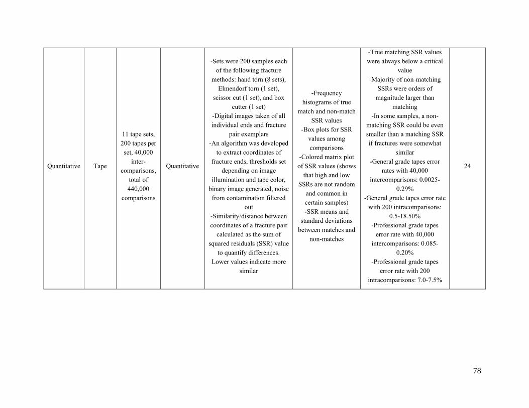
78
Quantitative Tape
11 tape sets,
200 tapes per
set, 40,000
inter-
comparisons,
total of
440,000
comparisons
Quantitative
-Sets were 200 samples each
of the following fracture
methods: hand torn (8 sets),
Elmendorf torn (1 set),
scissor cut (1 set), and box
cutter (1 set)
-Digital images taken of all
individual ends and fracture
pair exemplars
-An algorithm was developed
to extract coordinates of
fracture ends, thresholds set
depending on image
illumination and tape color,
binary image generated, noise
from contamination filtered
out
-Similarity/distance between
coordinates of a fracture pair
calculated as the sum of
squared residuals (SSR) value
to quantify differences.
Lower values indicate more
similar
-Frequency
histograms of true
match and non-match
SSR values
-Box plots for SSR
values among
comparisons
-Colored matrix plot
of SSR values (shows
that high and low
SSRs are not random
and common in
certain samples)
-SSR means and
standard deviations
between matches and
non-matches
-True matching SSR values
were always below a critical
value
-Majority of non-matching
SSRs were orders of
magnitude larger than
matching
-In some samples, a non-
matching SSR could be even
smaller than a matching SSR
if fractures were somewhat
similar
-General grade tapes error
rates with 40,000
intercomparisons: 0.0025-
0.29%
-General grade tapes error rate
with 200 intracomparisons:
0.5-18.50%
-Professional grade tapes
error rate with 40,000
intercomparisons: 0.085-
0.20%
-Professional grade tapes
error rate with 200
intracomparisons: 7.0-7.5%
24
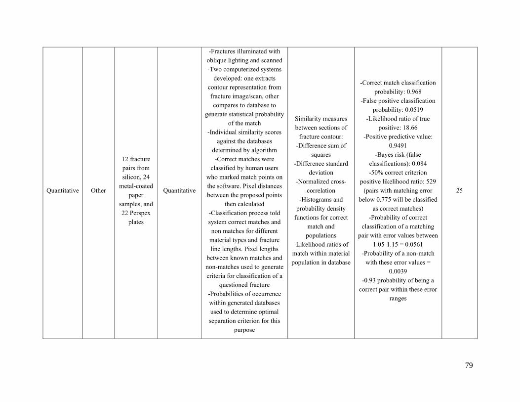
79
Quantitative Other
12 fracture
pairs from
silicon, 24
metal-coated
paper
samples, and
22 Perspex
plates
Quantitative
-Fractures illuminated with
oblique lighting and scanned
-Two computerized systems
developed: one extracts
contour representation from
fracture image/scan, other
compares to database to
generate statistical probability
of the match
-Individual similarity scores
against the databases
determined by algorithm
-Correct matches were
classified by human users
who marked match points on
the software. Pixel distances
between the proposed points
then calculated
-Classification process told
system correct matches and
non matches for different
material types and fracture
line lengths. Pixel lengths
between known matches and
non-matches used to generate
criteria for classification of a
questioned fracture
-Probabilities of occurrence
within generated databases
used to determine optimal
separation criterion for this
purpose
Similarity measures
between sections of
fracture contour:
-Difference sum of
squares
-Difference standard
deviation
-Normalized cross-
correlation
-Histograms and
probability density
functions for correct
match and
populations
-Likelihood ratios of
match within material
population in database
-Correct match classification
probability: 0.968
-False positive classification
probability: 0.0519
-Likelihood ratio of true
positive: 18.66
-Positive predictive value:
0.9491
-Bayes risk (false
classifications): 0.084
-50% correct criterion
positive likelihood ratio: 529
(pairs with matching error
below 0.775 will be classified
as correct matches)
-Probability of correct
classification of a matching
pair with error values between
1.05-1.15 = 0.0561
-Probability of a non-match
with these error values =
0.0039
-0.93 probability of being a
correct pair within these error
ranges
25
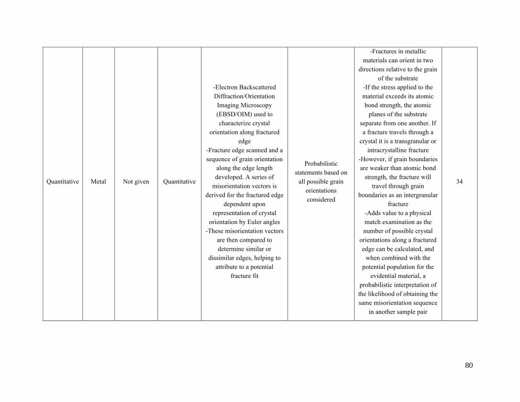
80
Quantitative Metal Not given Quantitative
-Electron Backscattered
Diffraction/Orientation
Imaging Microscopy
(EBSD/OIM) used to
characterize crystal
orientation along fractured
edge
-Fracture edge scanned and a
sequence of grain orientation
along the edge length
developed. A series of
misorientation vectors is
derived for the fractured edge
dependent upon
representation of crystal
orientation by Euler angles
-These misorientation vectors
are then compared to
determine similar or
dissimilar edges, helping to
attribute to a potential
fracture fit
Probabilistic
statements based on
all possible grain
orientations
considered
-Fractures in metallic
materials can orient in two
directions relative to the grain
of the substrate
-If the stress applied to the
material exceeds its atomic
bond strength, the atomic
planes of the substrate
separate from one another. If
a fracture travels through a
crystal it is a transgranular or
intracrystalline fracture
-However, if grain boundaries
are weaker than atomic bond
strength, the fracture will
travel through grain
boundaries as an intergranular
fracture
-Adds value to a physical
match examination as the
number of possible crystal
orientations along a fractured
edge can be calculated, and
when combined with the
potential population for the
evidential material, a
probabilistic interpretation of
the likelihood of obtaining the
same misorientation sequence
in another sample pair
34
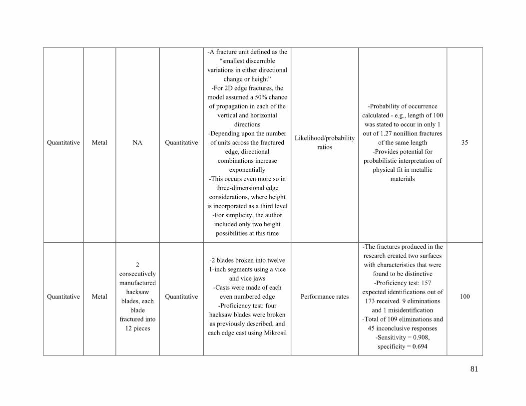
81
Quantitative Metal NA Quantitative
-A fracture unit defined as the
“smallest discernible
variations in either directional
change or height”
-For 2D edge fractures, the
model assumed a 50% chance
of propagation in each of the
vertical and horizontal
directions
-Depending upon the number
of units across the fractured
edge, directional
combinations increase
exponentially
-This occurs even more so in
three-dimensional edge
considerations, where height
is incorporated as a third level
-For simplicity, the author
included only two height
possibilities at this time
Likelihood/probability
ratios
-Probability of occurrence
calculated - e.g., length of 100
was stated to occur in only 1
out of 1.27 nonillion fractures
of the same length
-Provides potential for
probabilistic interpretation of
physical fit in metallic
materials
35
Quantitative Metal
2
consecutively
manufactured
hacksaw
blades, each
blade
fractured into
12 pieces
Quantitative
-2 blades broken into twelve
1-inch segments using a vice
and vice jaws
-Casts were made of each
even numbered edge
-Proficiency test: four
hacksaw blades were broken
as previously described, and
each edge cast using Mikrosil
Performance rates
-The fractures produced in the
research created two surfaces
with characteristics that were
found to be distinctive
-Proficiency test: 157
expected identifications out of
173 received. 9 eliminations
and 1 misidentification
-Total of 109 eliminations and
45 inconclusive responses
-Sensitivity = 0.908,
specificity = 0.694
100
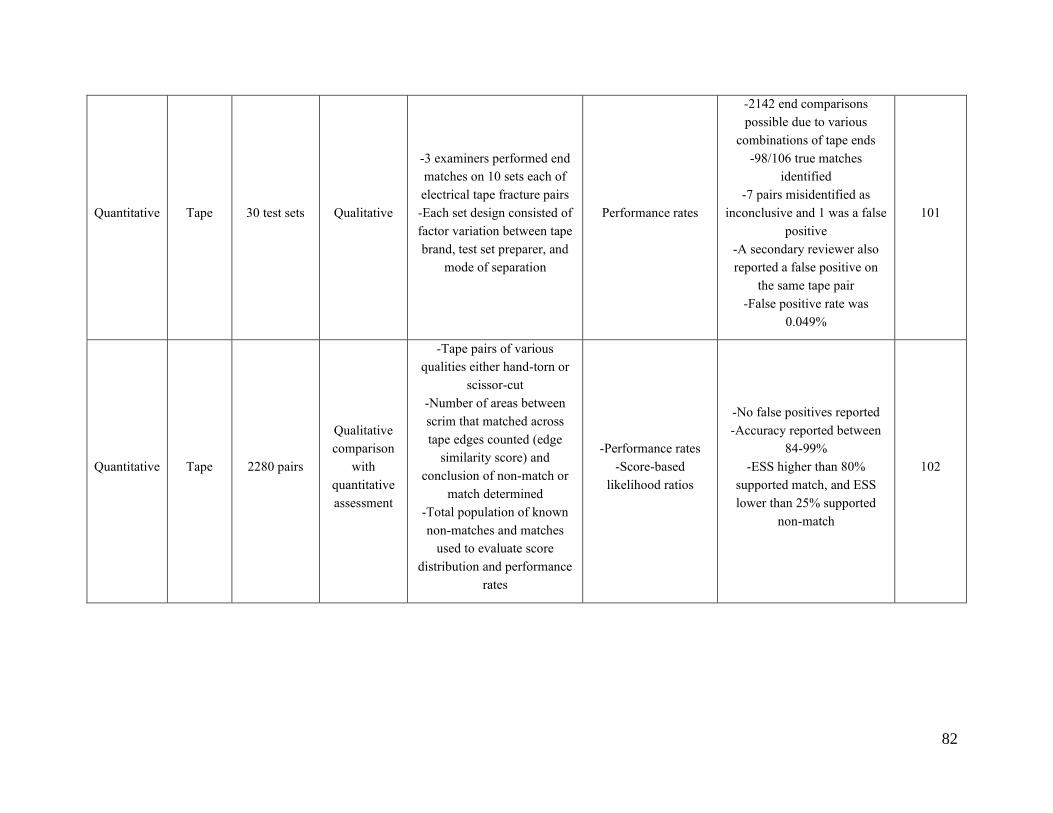
82
Quantitative Tape 30 test sets Qualitative
-3 examiners performed end
matches on 10 sets each of
electrical tape fracture pairs
-Each set design consisted of
factor variation between tape
brand, test set preparer, and
mode of separation
Performance rates
-2142 end comparisons
possible due to various
combinations of tape ends
-98/106 true matches
identified
-7 pairs misidentified as
inconclusive and 1 was a false
positive
-A secondary reviewer also
reported a false positive on
the same tape pair
-False positive rate was
0.049%
101
Quantitative Tape 2280 pairs
Qualitative
comparison
with
quantitative
assessment
-Tape pairs of various
qualities either hand-torn or
scissor-cut
-Number of areas between
scrim that matched across
tape edges counted (edge
similarity score) and
conclusion of non-match or
match determined
-Total population of known
non-matches and matches
used to evaluate score
distribution and performance
rates
-Performance rates
-Score-based
likelihood ratios
-No false positives reported
-Accuracy reported between
84-99%
-ESS higher than 80%
supported match, and ESS
lower than 25% supported
non-match
102
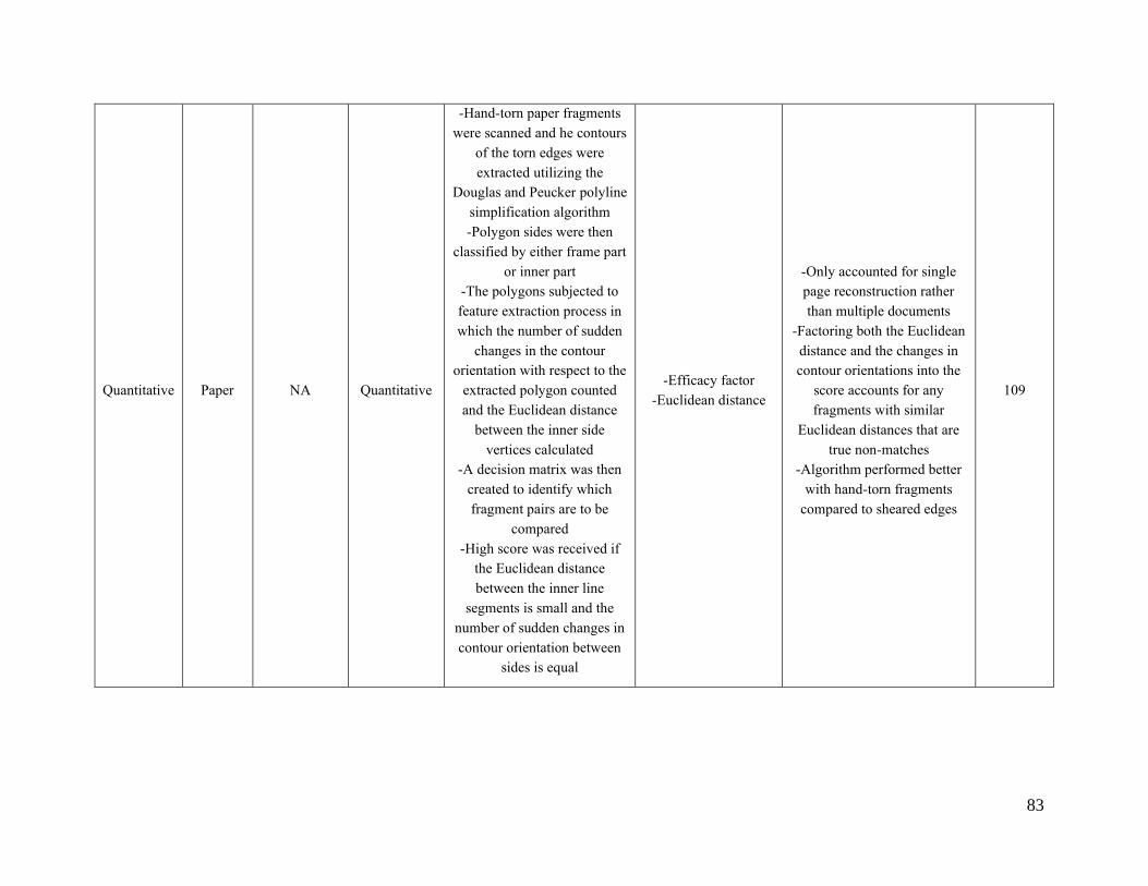
83
Quantitative Paper NA Quantitative
-Hand-torn paper fragments
were scanned and he contours
of the torn edges were
extracted utilizing the
Douglas and Peucker polyline
simplification algorithm
-Polygon sides were then
classified by either frame part
or inner part
-The polygons subjected to
feature extraction process in
which the number of sudden
changes in the contour
orientation with respect to the
extracted polygon counted
and the Euclidean distance
between the inner side
vertices calculated
-A decision matrix was then
created to identify which
fragment pairs are to be
compared
-High score was received if
the Euclidean distance
between the inner line
segments is small and the
number of sudden changes in
contour orientation between
sides is equal
-Efficacy factor
-Euclidean distance
-Only accounted for single
page reconstruction rather
than multiple documents
-Factoring both the Euclidean
distance and the changes in
contour orientations into the
score accounts for any
fragments with similar
Euclidean distances that are
true non-matches
-Algorithm performed better
with hand-torn fragments
compared to sheared edges
109
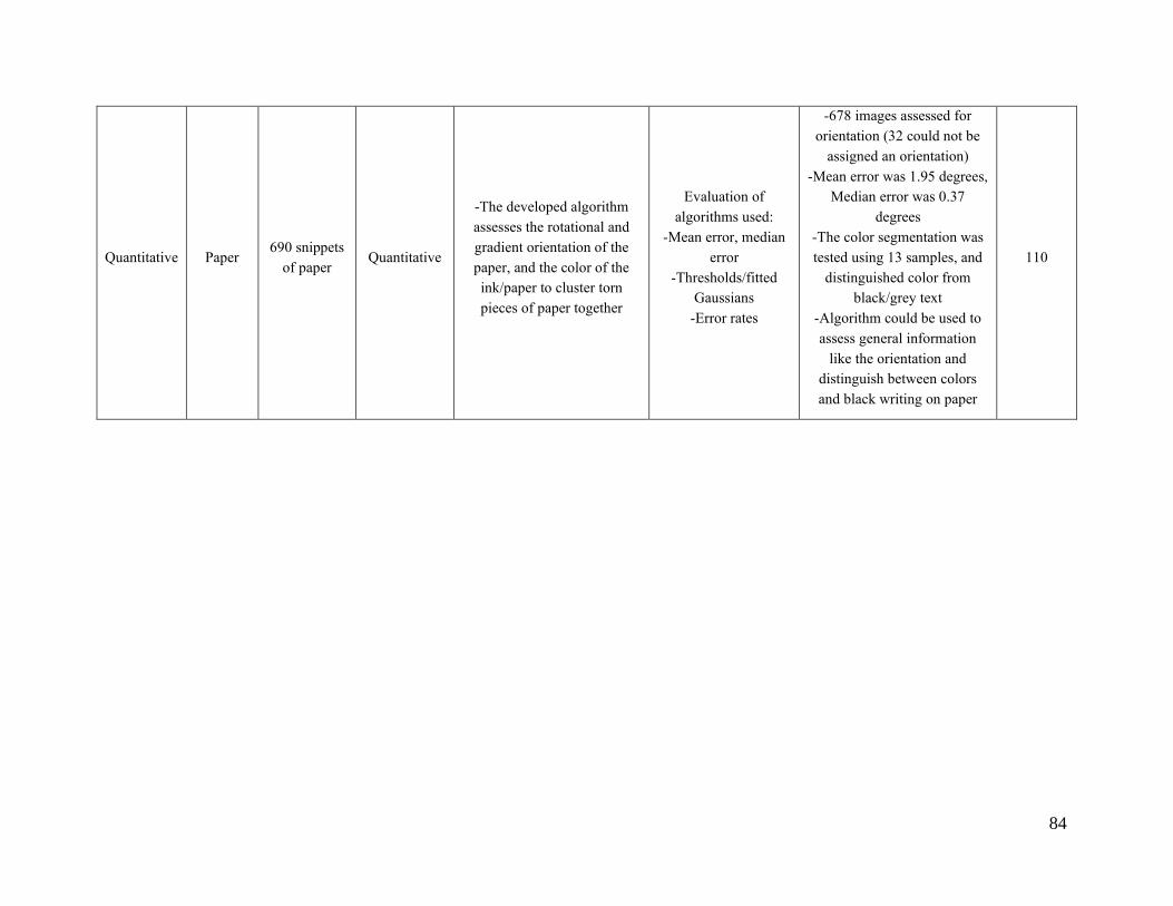
84
Quantitative Paper 690 snippets
of paper Quantitative
-The developed algorithm
assesses the rotational and
gradient orientation of the
paper, and the color of the
ink/paper to cluster torn
pieces of paper together
Evaluation of
algorithms used:
-Mean error, median
error
-Thresholds/fitted
Gaussians
-Error rates
-678 images assessed for
orientation (32 could not be
assigned an orientation)
-Mean error was 1.95 degrees,
Median error was 0.37
degrees
-The color segmentation was
tested using 13 samples, and
distinguished color from
black/grey text
-Algorithm could be used to
assess general information
like the orientation and
distinguish between colors
and black writing on paper
110
85
III. CHAPTER TWO
Inter-Laboratory Assessment of the Utility of the Edge Similarity Score (ESS)
in Duct Tape Physical Fit Examinations
1. Overview of the Inter-laboratory Study
As recent criticism of the forensic field has called for more quantitative methodology to reduce
subjectivity in comparative analyses1–3, it is becoming crucial to implement new comparison
methods to even the seemingly most straightforward of examinations, such as physical fit. To do
so, a critical component of the process towards validation and standardization of a new method is
to test it via inter-laboratory studies. This is done for purposes of establishing reproducibility and
reliability of a method for implementation into practice. These collaborative studies are also
effective to fine-tune the methods and arrive to consensus protocols.
In this project, an inter-laboratory study between trace evidence scientists was designed to assess
a quantitative, score-based physical fit technique, known as the edge similarity score (ESS) 4. This
interlaboratory collaboration was focused on the evaluation of the quality of duct tapes fractured
edges. A secondary purpose of this study was to evaluate the practitioners’ feedback on the method
for further improvements, which will be implemented in future collaborative exercises.
Incorporating the examiners’ comments on the applicability of the method is one of the essential
processes to generate approaches that are practical and likely to be implemented by the scientific
community.
As exact duct tape fractured edges cannot be experimentally reproduced, it was impractical to
provide the same fractured edges to every participant in a sequential circulation. Instead, physical
samples were created for each of three study kits in order to simulate items encountered in
casework. Each kit consisted of seven duct tape comparison pairs each, distributed in a Round-
Robin style to volunteer examiners at various federal, state, and local forensic laboratories. Each
kit contained four matching pairs (3 of them with a good quality match M+, one of them with a
weaker quality match M-) and 3 non-matching pairs (NM).
For each kit, the respective sample (e.g. sample 1 from Kits 1, 2 and 3) were prepared using the
same duct tape roll and the same separation method. Also, they were chosen to exhibit the same
macro edge pattern (e.g., puzzle, wavy or straight) and a similar ESS score. To establish maximum
similarity between kit samples, the comparison tapes were selected according to pre-distribution,
consensus ESS values established by four examiners. An agreement in the ESS better than ± 10%
ESS was used as the criteria for pre-distribution consensus. The average consensus ESS for true
good quality matches ranged from 86% to 99% (M+), true matches of lower alignment ranged
from 70% to 77% (M-), and non-matches ranged from 0% to 11% (NM), depending on the tape
sample.
86
As a means to reduce inter-examiner variability, participants were provided instructions in the
form of a detailed protocol document, and the majority also received an instructional presentation
on the ESS method to be used in their physical fit examinations. The study distribution resulted
in 16 completed kits overall, totaling 112 documented comparisons. Four approaches were used to
assess the ILS results. The first two approaches evaluated error rates based on pre-determined
thresholds or the overall examiner’s conclusion. The other two methods assessed the level of inter-
examiner agreement in reporting the edge similarity scores.
The overall performance and error rates were estimated based on two varying interpretations of
the reported ESS score and the respective correlation with the ground truth: 1) as per thresholds
established based on larger population datasets4 in which an ESS score below 50 was considered
a non-match, NM, and above 50, a match, M, and 2) as per the overall conclusion reported by the
examiners (Match, Inconclusive, or Non-match). Overall, the observed error rates in the ILS study
by threshold ESS values were 92% true positives (59/64), 8% false negatives (5/48), 100% true
negatives (48/48), and 0% false positives (0/64). Observed error rates by examiner-reported
conclusion were as follows: 95% true positives (61/64), 0% false negatives (0/48), 100% true
negatives (48/48), and 0% false positives (0/64). The reduction in the true positive rate is the result
of a 5% inconclusive rate (3 true positive samples were concluded as inconclusive across the
sample set).
Next, we evaluated how close the study participants reported the ESS and comparison edge
qualifiers in comparison to the consensus ranges. The majority (86.6%) of reported ESS scores
were within ± 20 ESS compared to consensus values determined before the administration of the
test, except for 15 out of 112 instances. We also observed that the majority (86 out of 112) of
reported ESS scores fell within expected comparison edge qualifier ranges as established in a
previous study by our research group4.
The proximity of reported ESS was also evaluated according to statistical significance testing via
Analysis of Variance with the Dunnett’s test at a 95% confidence interval. 77% of the reported
ESS showed no significant differences from the respective pre-distribution, consensus mean
scores. Interestingly, it was found that 8 of 11 individuals who reported significantly different ESS
scores from the consensus range received less instructional training.
ESS were also evaluated in terms of expected sample difficulty in relation to ground truth: true
positive samples of less expected difficulty in the upper qualifier range (M+, ESS between 80 and
100), true positive samples of more expected difficulty in the M- qualifier range (M-, ESS between
>50 and <80), and non-matching samples (NM, ESS <50). It was observed that within the M+ and
the NM groups, 81% of examiner ESS values were in agreement with consensus means according
to the Dunnett’s test. The M- group exhibited lower agreement of ESS scores according to
Dunnett’s (69% of values) which was expected due to increased examination difficulty. The
average ESS reported by participants for true good quality matches was 83 ± 17% (M+), 71 ± 19%
for M-, and 7 ± 11% for non-matches.

87
Three main observations were derived from the participant results: 1) overall good agreement
between ESS reported by examiners was observed, 2) the ESS score represented a good indicator
of the quality of the match and rendered low percent of error rates on conclusions 3) those
examiners that did not participate in formal method training tended to have ESS falling outside of
expected pre-distribution ranges. Also, the survey responses revealed that: 1) further training is
needed to standardize the reporting and interpretation of areas between scrim that contain less
features to evaluate, and 2) further training is also needed to establish consistency in terms of the
proper use of the comparison edge qualifier, as well as improving the understanding that the ESS
is only one step in the overall assessment of a fractured edge comparison pair.
These results indicate the ESS methodology allows for a high rate of inter-examiner agreement in
score value while still maintaining a correct pair classification (e.g., true match, true non-match)
overall. The prevalent observed trends, as well as feedback received through the post-study survey,
will be used to optimize the ESS methodology for the future development of a larger inter-
laboratory study which will be used to further validate the technique.
Most importantly, this pilot ILS represents the first time that a specific quantitative criterion is
used for end-tape physical fit examinations to support and inform the examiner's opinion, to
evaluate examiner error rates, and to provide a systematic peer review process. Indeed, most
respondents reported the ESS approach was useful for documenting the basis for their findings,
training new examiners, and allowing a transparent peer-review process. The implementation of
the method is therefore anticipated to increase objectivity and help to move towards consensus-
based guidelines.
2. Introduction
As covered in Chapter One, physical fits are considered the highest level of association between
two materials in trace evidence. However, recent reports from the National Academy of Sciences
(NAS)1 and President’s Council of Advisors on Science and Technology (PCAST),2 as well as a
statement from the American Statistical Association3 have called for further research into the
reporting of error rates and uncertainties associated with forensic analyses relying primarily upon
visual, feature-based comparisons. In terms of physical fits, this is a challenging task due to the
highly variable nature of circumstances faced in these examinations. To name a few, these varying
factors include material type, size, quantity, and fracture source.
An approach to assessing the performance of comparative methods is by evaluating error rates
observed in large datasets of known ground truth that are kept blind to the test takers. For duct tape
physical fits, performance rate studies have been demonstrated by Bradley et al. in which no false
positive or negatives were reported by any of the four participating examiners when assessing both
hand torn and scissor cut sample sets5. These studies have also been shared by Tulleners and Braun
in which low examiner error rates were demonstrated in an expanded sample set (≥1600 samples)
of various separation methods including hand torn, Elmendorf torn, scissor cut, and box cutter
knife cut. Overall, the accuracy rate ranged from 98.15-100% depending on separation method,
88
while the false positive rate ranged from 0.00-3.33%, and the false negative rate ranged from 0.00-
2.67%6.
Most recently, a study by Prusinowski et al.4 introduced an alternative method to obtain a similarity
score for a duct tape physical fit pair. The proposed method involves a relative percentage of
consistent scrim areas along the total width of a tape pair, referred to as an edge similarity score
(ESS) as demonstrated in Equation 1 below.
𝐸𝑑𝑔𝑒 𝑠𝑖𝑚𝑖𝑙𝑎𝑟𝑖𝑡𝑦 𝑠𝑐𝑜𝑟𝑒 (𝐸𝑆𝑆) = 𝑁𝑢𝑚𝑏𝑒𝑟 𝑜𝑓 𝑐𝑜𝑛𝑠𝑖𝑠𝑡𝑒𝑛𝑡 𝑠𝑐𝑟𝑖𝑚 𝑎𝑟𝑒𝑎𝑠
𝑇𝑜𝑡𝑎𝑙 𝑛𝑢𝑚𝑏𝑒𝑟 𝑜𝑓 𝑠𝑐𝑟𝑖𝑚 𝑎𝑟𝑒𝑎𝑠∗ 100 (1)
Within the Prusinowski study4, a set of 2280 duct tape ESS were obtained from student examiners
kept blind to sample ground truth for low, medium, and high-grade tapes of both hand torn and
scissor cut separation methods. The resulting scores were evaluated in terms of performance rates.
No false positives were observed in any of the sets and examiner accuracy ranged from 84.9% to
over 99.0%. The study also utilized the score likelihood ratio as a quantitative interpretation of the
ESS within the sample set.4 This study demonstrated for the first time a systematic, quantitative
method of score-based assessment of duct tape physical fits. This method provides several
advantages including: 1) a method by which to inform the practitioner’s opinion in difficult item
alignment situations, 2) a method of providing further support to the practitioner’s opinion of the
physical fit, 3) the development of systematic criteria for a more transparent peer review process,
4) a method to assess experimental error rates, and 5) a means to assess factors that influence the
quality of a fit.
Following the development of the ESS method for duct tape physical fit examinations by our
research group, the expanding goals of the study included steps towards implementation of the
method into forensic laboratories. Before implementation can occur, extensive verification of the
method’s utility, validity, reliability, and reproducibility between different examiners as well as
different laboratories must be assessed. An effective approach for such assessment is via an inter-
laboratory study. According to ISO/IEC 17043,7 these studies serve to evaluate methods or tests
on the same or similar items by two or more laboratories in accordance with predetermined
conditions. Inter-laboratory comparisons are utilized in several scientific disciplines such as
biotechnology, environmental science, food science, forensics, and medicine.8–12 Purposes for
inter-laboratory studies can take several forms. One of which is to establish reproducibility of a
single analytical method as part of a validation process. These studies are referred to as
collaborative trials or method performance studies.13 Inter-laboratory comparisons can also be
utilized to reach a consensus on the characterization of a standard reference material or a protocol
of analysis or interpretation, as is often reported in ASTM standard test methods. For example,
ASTM E17714 and E69115 describe practices for the use of precision and bias in test methods and
how to conduct an interlaboratory study to determine intra and inter-lab precision, respectively.
Further, inter-laboratory studies can also be initiated for methods already standardized and
routinely used in laboratories. This is done for purposes of laboratory performance assessment and
identification of bias originating from either the method or between laboratories. This type of
comparison is known as proficiency testing or laboratory performance studies.13
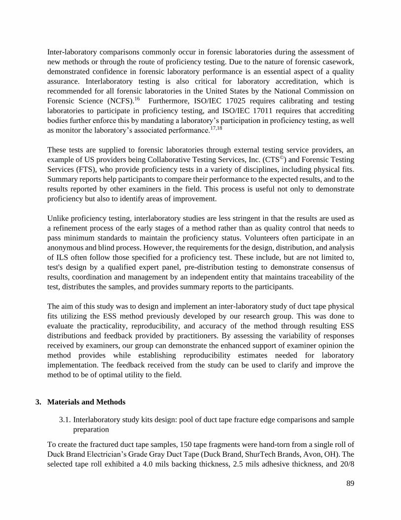
89
Inter-laboratory comparisons commonly occur in forensic laboratories during the assessment of
new methods or through the route of proficiency testing. Due to the nature of forensic casework,
demonstrated confidence in forensic laboratory performance is an essential aspect of a quality
assurance. Interlaboratory testing is also critical for laboratory accreditation, which is
recommended for all forensic laboratories in the United States by the National Commission on
Forensic Science (NCFS).16 Furthermore, ISO/IEC 17025 requires calibrating and testing
laboratories to participate in proficiency testing, and ISO/IEC 17011 requires that accrediting
bodies further enforce this by mandating a laboratory’s participation in proficiency testing, as well
as monitor the laboratory’s associated performance.17,18
These tests are supplied to forensic laboratories through external testing service providers, an
example of US providers being Collaborative Testing Services, Inc. (CTS©) and Forensic Testing
Services (FTS), who provide proficiency tests in a variety of disciplines, including physical fits.
Summary reports help participants to compare their performance to the expected results, and to the
results reported by other examiners in the field. This process is useful not only to demonstrate
proficiency but also to identify areas of improvement.
Unlike proficiency testing, interlaboratory studies are less stringent in that the results are used as
a refinement process of the early stages of a method rather than as quality control that needs to
pass minimum standards to maintain the proficiency status. Volunteers often participate in an
anonymous and blind process. However, the requirements for the design, distribution, and analysis
of ILS often follow those specified for a proficiency test. These include, but are not limited to,
test's design by a qualified expert panel, pre-distribution testing to demonstrate consensus of
results, coordination and management by an independent entity that maintains traceability of the
test, distributes the samples, and provides summary reports to the participants.
The aim of this study was to design and implement an inter-laboratory study of duct tape physical
fits utilizing the ESS method previously developed by our research group. This was done to
evaluate the practicality, reproducibility, and accuracy of the method through resulting ESS
distributions and feedback provided by practitioners. By assessing the variability of responses
received by examiners, our group can demonstrate the enhanced support of examiner opinion the
method provides while establishing reproducibility estimates needed for laboratory
implementation. The feedback received from the study can be used to clarify and improve the
method to be of optimal utility to the field.
3. Materials and Methods
3.1. Interlaboratory study kits design: pool of duct tape fracture edge comparisons and sample
preparation
To create the fractured duct tape samples, 150 tape fragments were hand-torn from a single roll of
Duck Brand Electrician’s Grade Gray Duct Tape (Duck Brand, ShurTech Brands, Avon, OH). The
selected tape roll exhibited a 4.0 mils backing thickness, 2.5 mils adhesive thickness, and 20/8
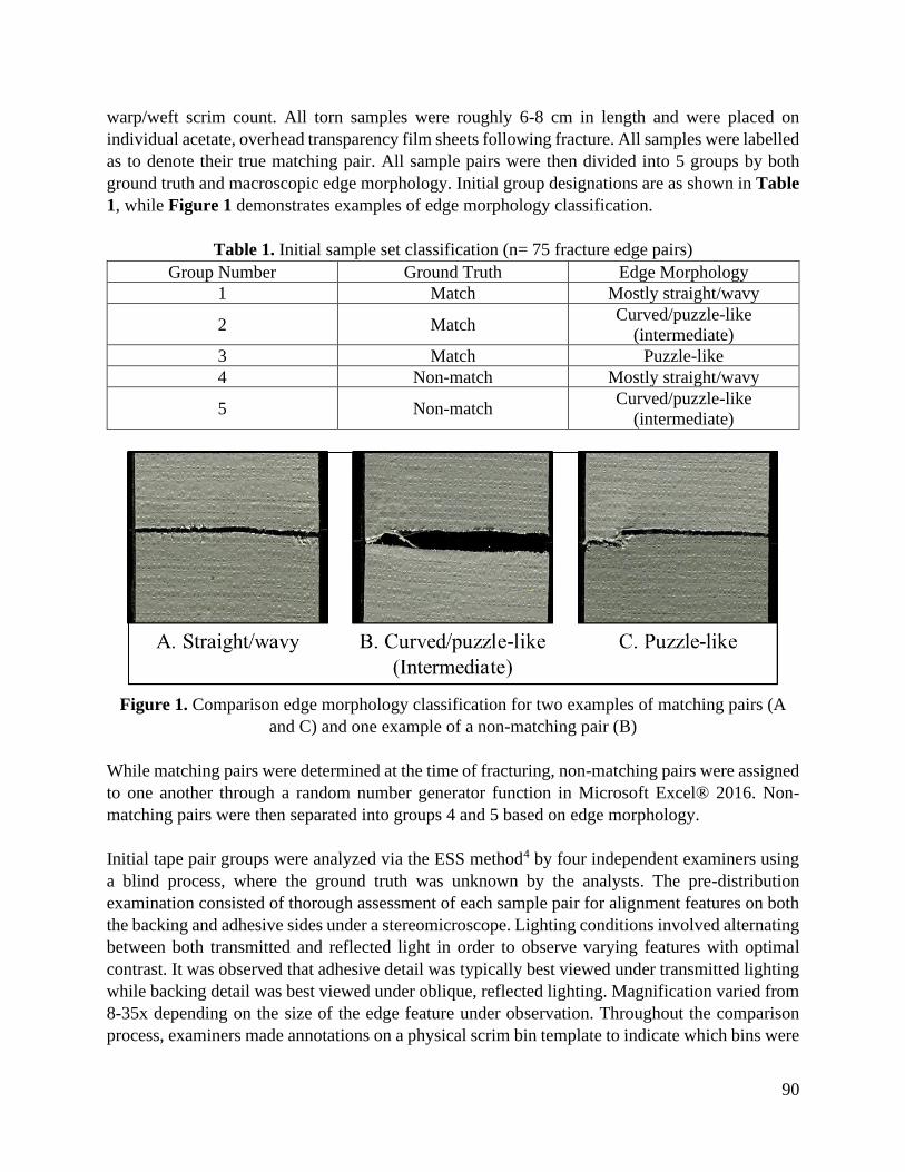
90
warp/weft scrim count. All torn samples were roughly 6-8 cm in length and were placed on
individual acetate, overhead transparency film sheets following fracture. All samples were labelled
as to denote their true matching pair. All sample pairs were then divided into 5 groups by both
ground truth and macroscopic edge morphology. Initial group designations are as shown in Table
1, while Figure 1 demonstrates examples of edge morphology classification.
Table 1. Initial sample set classification (n= 75 fracture edge pairs)
Group Number Ground Truth Edge Morphology
1 Match Mostly straight/wavy
2 Match Curved/puzzle-like
(intermediate)
3 Match Puzzle-like
4 Non-match Mostly straight/wavy
5 Non-match Curved/puzzle-like
(intermediate)
Figure 1. Comparison edge morphology classification for two examples of matching pairs (A
and C) and one example of a non-matching pair (B)
While matching pairs were determined at the time of fracturing, non-matching pairs were assigned
to one another through a random number generator function in Microsoft Excel® 2016. Non-
matching pairs were then separated into groups 4 and 5 based on edge morphology.
Initial tape pair groups were analyzed via the ESS method4 by four independent examiners using
a blind process, where the ground truth was unknown by the analysts. The pre-distribution
examination consisted of thorough assessment of each sample pair for alignment features on both
the backing and adhesive sides under a stereomicroscope. Lighting conditions involved alternating
between both transmitted and reflected light in order to observe varying features with optimal
contrast. It was observed that adhesive detail was typically best viewed under transmitted lighting
while backing detail was best viewed under oblique, reflected lighting. Magnification varied from
8-35x depending on the size of the edge feature under observation. Throughout the comparison
process, examiners made annotations on a physical scrim bin template to indicate which bins were
91
considered consistent (“1” = match) and inconsistent (“0” = non-match). The templates allowed
for a more transparent discussion and review process when comparing examiner results to assess
which samples resulted in the highest consensus in their ESS results. For a more detailed
description of the edge features commonly assessed as well as the ESS method, please refer to
Section 3.3 below.
Comparison pairs resulting in inter-examiner ESS relative standard deviations greater than 10%
ESS were eliminated from the sample set as potential inter-laboratory kit sample. The remaining
sample pairs meeting examiner agreement criteria were further rearranged into seven groups of
three similar pairs each, to prepare 3 kits of seven comparison pairs. Classification of the seven
optimized groups is provided in Table 2.
Table 2. Optimized sample set classification
Group Number
(n= 3 tape pairs per
group)
Ground Truth
Expected
Comparison Edge
Qualifier
Edge Morphology
1 Match M+ Straight/wavy
2 Match M- Puzzle-like
3 Match M+ Puzzle-like
4 Non-match NM+ Straight/wavy
5 Non-match NM+ Curved/puzzle-like
(intermediate)
6 Match M+ Puzzle-like
7 Non-match NM+ Straight/wavy
Kits were composed of one pair per optimized group. The pre-distribution score means provided
a baseline for expected participant ESS values. The matching pairs consisted of 3 pairs with
consensus ESS ranging from 86% to 99% (M+) and one more difficult match pair with consensus
ESS scores ranging from 70% to 77% (M-); while the non-matching (NM) pairs had consensus
scores from 0% to 11%. The desired participant agreement threshold was set for ± 20% from the
consensus mean.
3.2. Design of test distribution
The study kits consisted of the seven duct tape comparison pairs, a printed document outlining
method protocol, and hard-copy templates for score documentation. Along with the physical kits
sent by mail, participants received via email an instructional presentation, a digital copy of the
protocol, and a digital template containing tabs for score documentation of each comparison pair.
The final tab of the digital template file contained a post-study survey for each participant. Copies
of these documents are provided in Appendix A. In addition, many study participants were present
at a formal presentation of the proposed comparison method at which physical samples (none being
used in the study kits) were available for hands-on instruction. Further, at the time of distribution,
each participant was offered additional explanation of the protocol via phone or video conference.
92
Study kits were distributed in a modified petal test design in which each kit would return to the
coordination body before being re-distributed to the next participant as a Round Robin. A
schematic of the study design is provided in Figure 2.
Figure 2. Inter-laboratory modified petal test distribution
We aimed for 7 participants per kit. However, due to uncontrolled circumstances, Kit 1 had six
total participants, Kit 2 had three total participants, and Kit 3 had seven total participants. As kits
were returned, sample pairs were examined under a stereomicroscope to assure tapes had not been
manipulated or written upon before re-packaging the kit for continued distribution. The study
distribution design allowed for simultaneous distribution of each of the three kits. Distribution
took place over a period of about nine months. All participants were asked for a turnaround time
of 3-4 weeks, although several took longer.
3.3. Reporting instructions
Participants were asked to follow the ESS method as outlined in Prusinowski et al.4 Within this
method, participants begin their assessment by a general stereoscopic examination of both the
backing and adhesive sides of a duct tape pair. For purposes of the inter-laboratory study,
participants were given the specific physical feature examples of dimpling, calendering striae,
backing distortion, warp scrim alignment, protruding warp yarns, adhesive distortion, continuation
of scrim pattern, double weft edge scrim, and missing scrim to assess during their initial physical
examinations. Images of the provided feature examples are shown in Figures 3 and 4 below.
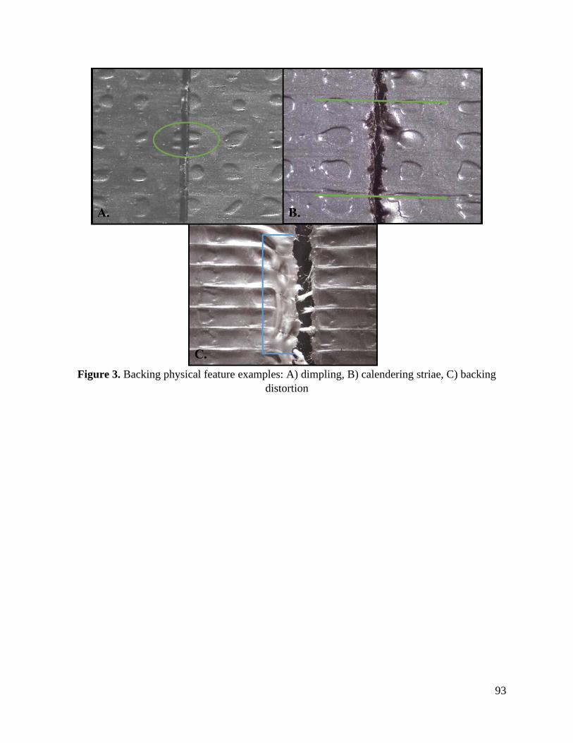
93
Figure 3. Backing physical feature examples: A) dimpling, B) calendering striae, C) backing
distortion
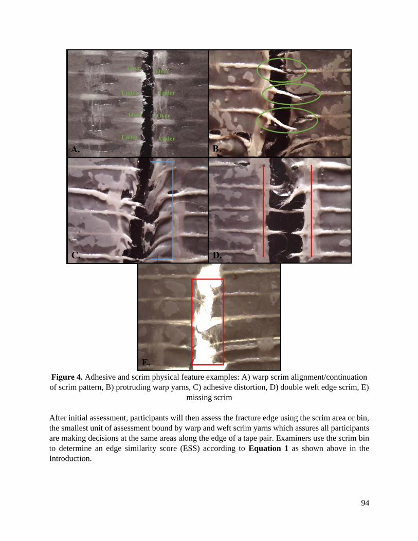
94
Figure 4. Adhesive and scrim physical feature examples: A) warp scrim alignment/continuation
of scrim pattern, B) protruding warp yarns, C) adhesive distortion, D) double weft edge scrim, E)
missing scrim
After initial assessment, participants will then assess the fracture edge using the scrim area or bin,
the smallest unit of assessment bound by warp and weft scrim yarns which assures all participants
are making decisions at the same areas along the edge of a tape pair. Examiners use the scrim bin
to determine an edge similarity score (ESS) according to Equation 1 as shown above in the
Introduction.
95
Participants then determined comparison edge qualifiers and comparison pair overall conclusions
with options as shown in Table 3 below:
Table 3. Options for comparison pair overall conclusion and qualifiers, as well as expected ESS
ranges per qualifier
Comparison Pair Overall
Conclusion Comparison Edge Qualifier
Expected ESS Range per
Qualifier4
1 = Match M+ = Match with high
certainty 80% – 100%
INC = Inconclusive M- = Match with low certainty 50% – < 80%
0 = Non-match INC = Inconclusive ~ 50%
NM- = Non-match with low
certainty 25% – < 50%
NM+ = Non-match with high
certainty 0% – ≤ 25%
Table 3 above outlines expected ranges of ESS per qualifier according to previous SLR ranges in
a publication by Prusinowski et al.4. In the study, assessment of duct tape ESS via the score
likelihood ratio (SLR) revealed that most ESS greater than 80% resulted in SLRs supporting a
match conclusion, while ESS lower than 25% resulted in SLRs supporting a non-match conclusion.
Samples were purposefully selected for the study kits that had been assigned a variation of ESS
ranges in order to provide a range of scenarios for participants.
3.4. Assessment of the inter-laboratory results
Results were assessed through four main avenues: 1-2) error rate assessment based on pre-
determined thresholds or the overall examiner’s conclusion, 3) ESS and qualifier consensus range
analysis, and 4) distribution and statistical analysis of ESS as grouped by expected comparison
difficulty in relation to ground truth. Each approach is outlined in further detail below. All
calculations and range assessments were performed in Microsoft Excel (Version 19.08), while
statistical analysis through Dunnett’s testing was performed in JMP Pro 13 (v.2016, SAS Institute
Inc., NC).
3.4.1. Performance rate assessment
The first assessment of study results was via performance rates including true positive rate (TPR),
true negative rate (TNR), false positive rate (FPR), false negative rate (FNR), inconclusive rate,
sensitivity, specificity, and accuracy. All rates were calculated according to the respective
equations in Table 4.
96
Table 4. Performance rate equation summary
Performance rate Equation
True Positive Rate (TPR)
𝑇𝑃𝑅 = 𝑇𝑃
𝑇𝑃+𝐹𝑁+𝐼𝑁𝐶 * 100
True Negative Rate (TNR)
𝑇𝑁𝑅 = 𝑇𝑁
𝑇𝑁+𝐹𝑃+𝐼𝑁𝐶 * 100
False Positive Rate (FPR)
𝐹𝑃𝑅 = 𝐹𝑃
𝐹𝑃+𝑇𝑁+𝐼𝑁𝐶 * 100
False Negative Rate (FNR)
𝐹𝑁𝑅 = 𝐹𝑁
𝑇𝑃+𝐹𝑁+𝐼𝑁𝐶 * 100
Inconclusive Rate (TP)
𝐼𝑁𝐶 = 𝐼𝑁𝐶
𝑇𝑃+𝐹𝑁+𝐼𝑁𝐶 * 100
Sensitivity
𝑆𝑒𝑛𝑠𝑖𝑡𝑖𝑣𝑖𝑡𝑦 = 𝑇𝑃
𝑇𝑃+𝐹𝑁 * 100
Specificity
𝑆𝑝𝑒𝑐𝑖𝑓𝑖𝑐𝑖𝑡𝑦 = 𝑇𝑁
𝑇𝑁+𝐹𝑃 * 100
Accuracy
𝐴𝑐𝑐𝑢𝑟𝑎𝑐𝑦 = 𝑇𝑃+𝑇𝑁
𝑇𝑃+𝑇𝑁+𝐹𝑃+𝐹𝑁+𝐼𝑁𝐶 * 100
Performance rates were assessed in two different interpretations: 1) according to a pre-established4
match/non-match ESS threshold in which ESS < 50% indicate a non-match result and ESS > 50%
indicate a match result or 2) according to assigned overall examiner conclusion of match, non-
match, or inconclusive – regardless of determined ESS value.
3.4.2. ESS and qualifier consensus range analysis
Resulting ESS distributions per kit were also examined to assess if scores fit within the pre-
determined ± 20 threshold versus the consensus mean, and that participants were in agreement
with the ground truth (e.g., match versus non-match). Distributions of comparison edge qualifiers
between kits were also examined to observe if participant qualifiers fell within expected ranges as
outlined in Table 3 above.
3.4.3. ESS as grouped by expected comparison difficulty and ground truth
ESS results were also assessed by grouping the resulting values in terms of the expected
comparison difficulty in relation to ground truth: true positive samples of less expected difficulty
(M+ qualifier range, M+), true positive samples of more expected difficulty (M- qualifier range,
M-) and non-matching samples (NM). ESS distributions per group are examined through boxplots.
Following exploratory ESS variation analysis, descriptive statistics were reported and Analysis of
Variance (ANOVA) for a Randomized Complete Block Design (RBCD) was performed on the
data to determine if significant differences existed between examiner results and the pre-
distribution, consensus mean per difficulty grouping. This was done specifically through the utility
of the Dunnett’s test, which compares individual sample means to an established control mean to
determine if any statistically significant differences arise.
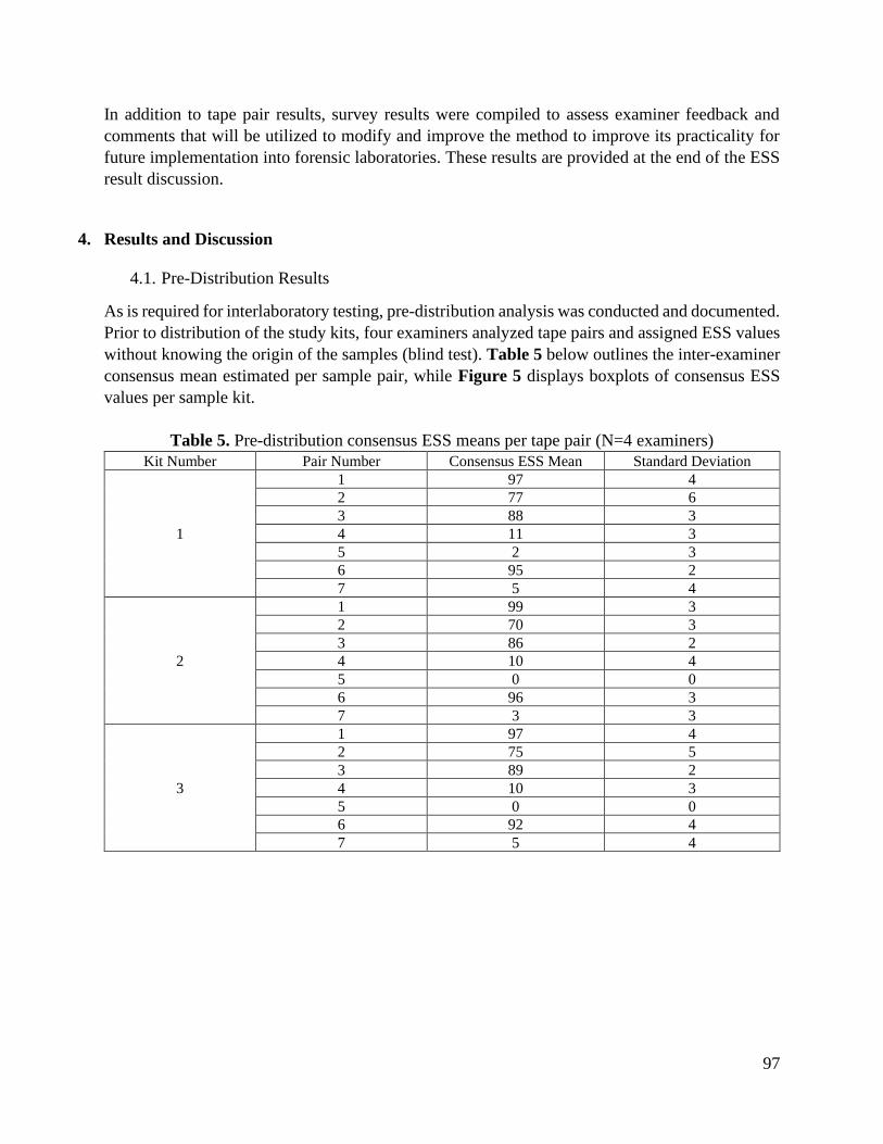
97
In addition to tape pair results, survey results were compiled to assess examiner feedback and
comments that will be utilized to modify and improve the method to improve its practicality for
future implementation into forensic laboratories. These results are provided at the end of the ESS
result discussion.
4. Results and Discussion
4.1. Pre-Distribution Results
As is required for interlaboratory testing, pre-distribution analysis was conducted and documented.
Prior to distribution of the study kits, four examiners analyzed tape pairs and assigned ESS values
without knowing the origin of the samples (blind test). Table 5 below outlines the inter-examiner
consensus mean estimated per sample pair, while Figure 5 displays boxplots of consensus ESS
values per sample kit.
Table 5. Pre-distribution consensus ESS means per tape pair (N=4 examiners)
Kit Number Pair Number Consensus ESS Mean Standard Deviation
1
1 97 4
2 77 6
3 88 3
4 11 3
5 2 3
6 95 2
7 5 4
2
1 99 3
2 70 3
3 86 2
4 10 4
5 0 0
6 96 3
7 3 3
3
1 97 4
2 75 5
3 89 2
4 10 3
5 0 0
6 92 4
7 5 4
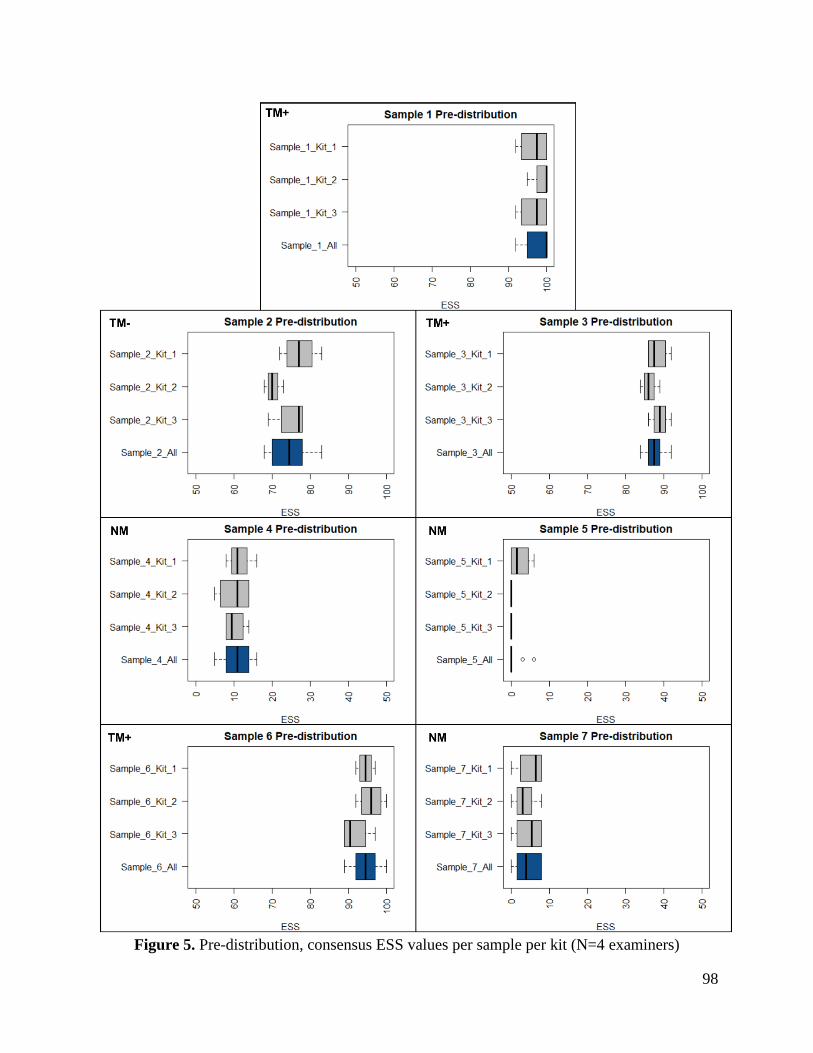
98
Figure 5. Pre-distribution, consensus ESS values per sample per kit (N=4 examiners)
99
As observed in Table 5 and Figure 5, sample pairs were selected for use in the study kits in which
the consensus mean had a standard deviation value lower than 10. In addition, samples were
selected such that each respective pair would be of similar edge morphology and expected ESS
range to its equivalent pair in all study kits. Sample groups were also assigned expected
comparison edge qualifier ranges due to previously reported threshold values4. Table 6 below
displays selected edge morphology, ground truth, expected qualifier range, and mean ESS across
equivalent samples per kit.
Table 6. Sample group pre-distribution characteristics across samples between the 3 kits Sample
group 1 2 3 4 5 6 7
Edge
morphology
Mostly
straight/wavy
Puzzle-
like
Puzzle-
like
Mostly
straight/wavy
Curved/puzzle-
like
(intermediate)
Puzzle-
like
Mostly
straight/wavy
Ground
truth Match Match Match Non-match Non-match Match Non-match
Expected
qualifier
range
M+ M- M+ NM+ NM+ M+ NM+
Mean ESS
across kits 97 74 88 11 1 94 4
ESS
standard
deviation
1 4 1 1 1 2 1
4.2. Performance Rate Assessment
Performance rates were considered through two main interpretations: 1) according to thresholds
established based on larger population datasets4 in which an ESS score below 50 was considered
NM, and above 50 M, and 2) according to the conclusion reported by the examiners (“1” = Match,
“INC” = Inconclusive, “0” = Non-match). For each avenue, true positive rate (TPR), true negative
rate (TNR), false positive rate (FPR), false negative rate (FNR), inconclusive rate (INC),
sensitivity, specificity, and accuracy per kit were calculated according to the equations in Table 4.
It should be noted that in this study there were three inconclusive conclusions, all of which were
true match samples. Table 7 below provides TPR, TNR, FPR, FNR, INC, sensitivity, specificity,
and accuracy rates overall and per kit for both overall examiner conclusion as well as conclusions
by ESS based on the expected 50/50 non-match/match threshold. As observed, accuracy rates by
examiner conclusion ranged between 90 and 100% across all kits with low error rates. Accuracy
rates by ESS threshold ranged between 88 and 10% with error rates ranging from 0-21%. Higher
error rates arose with Kits 1 and 2, thereby also affecting the overall error rates. When considering
Kit 1 classifications by ESS threshold, there were five samples with ESS scores reported below
50% that were still concluded as matches. However, this decreased the TPR and increased the
FNR. Kits 1 and 2 exhibited the presence of inconclusive conclusions by the examiner for true
match samples (1 within kit 1 and 2 within kit 2). While not necessarily a misclassification, this
caused a slight decrease in the accuracy and TPR for each kit.
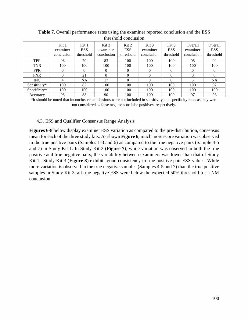
100
Table 7. Overall performance rates using the examiner reported conclusion and the ESS
threshold conclusion
Kit 1
examiner
conclusion
Kit 1
ESS
threshold
Kit 2
examiner
conclusion
Kit 2
ESS
threshold
Kit 3
examiner
conclusion
Kit 3
ESS
threshold
Overall
examiner
conclusion
Overall
ESS
threshold
TPR 96 79 83 100 100 100 95 92
TNR 100 100 100 100 100 100 100 100
FPR 0 0 0 0 0 0 0 0
FNR 0 21 0 0 0 0 0 8
INC 4 NA 17 0 0 0 5 NA
Sensitivity* 100 82 100 100 100 100 100 92
Specificity* 100 100 100 100 100 100 100 100
Accuracy 98 88 90 100 100 100 97 96
*It should be noted that inconclusive conclusions were not included in sensitivity and specificity rates as they were
not considered as false negatives or false positives, respectively.
4.3. ESS and Qualifier Consensus Range Analysis
Figures 6-8 below display examiner ESS variation as compared to the pre-distribution, consensus
mean for each of the three study kits. As shown Figure 6, much more score variation was observed
in the true positive pairs (Samples 1-3 and 6) as compared to the true negative pairs (Sample 4-5
and 7) in Study Kit 1. In Study Kit 2 (Figure 7), while variation was observed in both the true
positive and true negative pairs, the variability between examiners was lower than that of Study
Kit 1. Study Kit 3 (Figure 8) exhibits good consistency in true positive pair ESS values. While
more variation is observed in the true negative samples (Samples 4-5 and 7) than the true positive
samples in Study Kit 3, all true negative ESS were below the expected 50% threshold for a NM
conclusion.
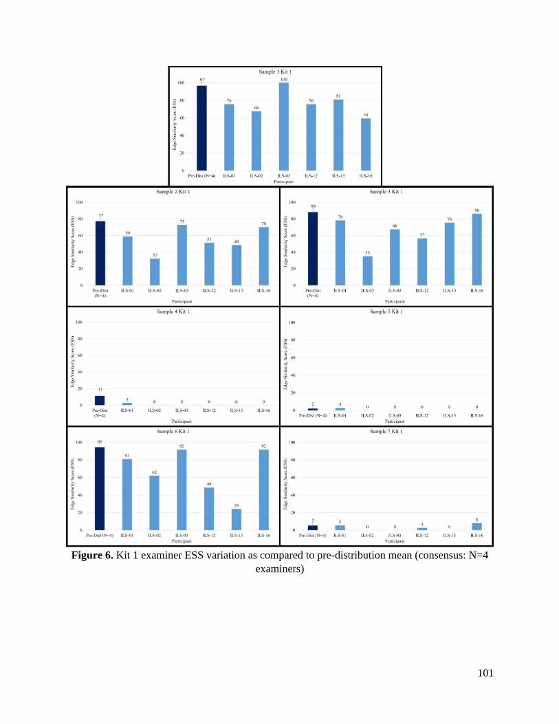
101
Figure 6. Kit 1 examiner ESS variation as compared to pre-distribution mean (consensus: N=4
examiners)
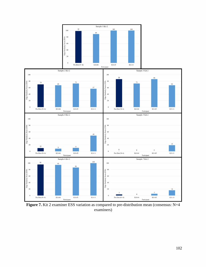
102
Figure 7. Kit 2 examiner ESS variation as compared to pre-distribution mean (consensus: N=4
examiners)
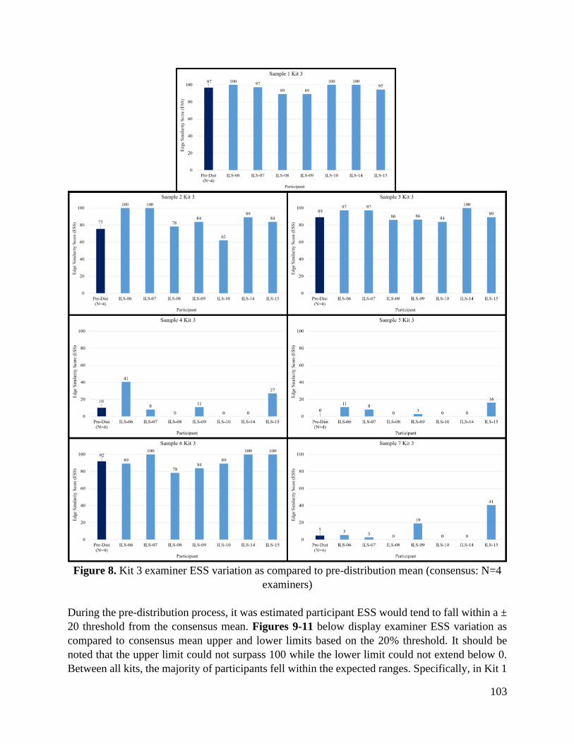
103
Figure 8. Kit 3 examiner ESS variation as compared to pre-distribution mean (consensus: N=4
examiners)
During the pre-distribution process, it was estimated participant ESS would tend to fall within a ±
20 threshold from the consensus mean. Figures 9-11 below display examiner ESS variation as
compared to consensus mean upper and lower limits based on the 20% threshold. It should be
noted that the upper limit could not surpass 100 while the lower limit could not extend below 0.
Between all kits, the majority of participants fell within the expected ranges. Specifically, in Kit 1
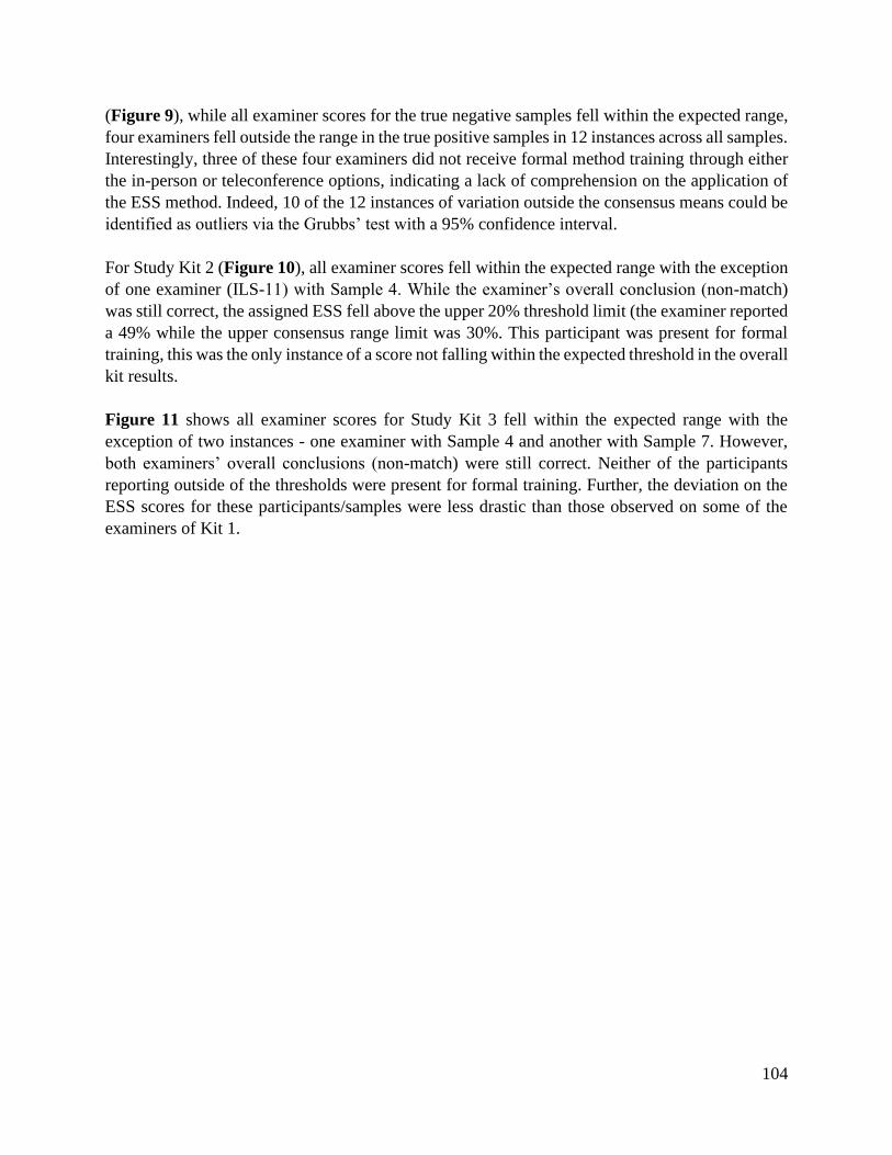
104
(Figure 9), while all examiner scores for the true negative samples fell within the expected range,
four examiners fell outside the range in the true positive samples in 12 instances across all samples.
Interestingly, three of these four examiners did not receive formal method training through either
the in-person or teleconference options, indicating a lack of comprehension on the application of
the ESS method. Indeed, 10 of the 12 instances of variation outside the consensus means could be
identified as outliers via the Grubbs’ test with a 95% confidence interval.
For Study Kit 2 (Figure 10), all examiner scores fell within the expected range with the exception
of one examiner (ILS-11) with Sample 4. While the examiner’s overall conclusion (non-match)
was still correct, the assigned ESS fell above the upper 20% threshold limit (the examiner reported
a 49% while the upper consensus range limit was 30%. This participant was present for formal
training, this was the only instance of a score not falling within the expected threshold in the overall
kit results.
Figure 11 shows all examiner scores for Study Kit 3 fell within the expected range with the
exception of two instances - one examiner with Sample 4 and another with Sample 7. However,
both examiners’ overall conclusions (non-match) were still correct. Neither of the participants
reporting outside of the thresholds were present for formal training. Further, the deviation on the
ESS scores for these participants/samples were less drastic than those observed on some of the
examiners of Kit 1.
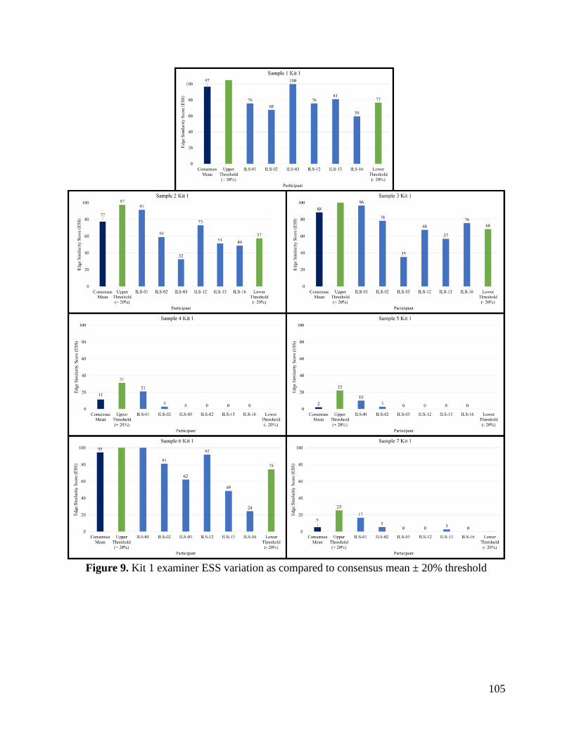
105
Figure 9. Kit 1 examiner ESS variation as compared to consensus mean ± 20% threshold
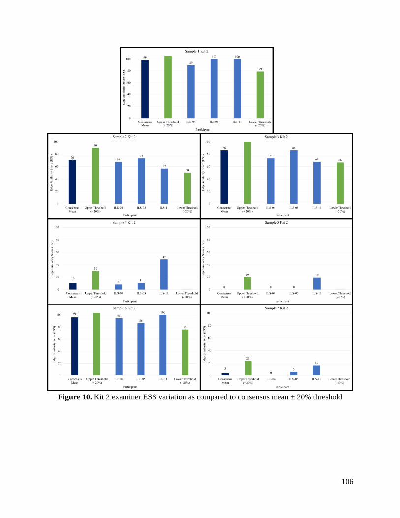
106
Figure 10. Kit 2 examiner ESS variation as compared to consensus mean ± 20% threshold
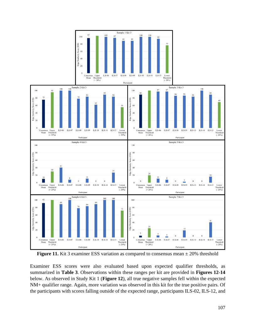
107
Figure 11. Kit 3 examiner ESS variation as compared to consensus mean ± 20% threshold
Examiner ESS scores were also evaluated based upon expected qualifier thresholds, as
summarized in Table 3. Observations within these ranges per kit are provided in Figures 12-14
below. As observed in Study Kit 1 (Figure 12), all true negative samples fell within the expected
NM+ qualifier range. Again, more variation was observed in this kit for the true positive pairs. Of
the participants with scores falling outside of the expected range, participants ILS-02, ILS-12, and
108
ILS-13 provided ESS that were consistently lower than the expected range. As mentioned earlier,
this seems to be a result of lack of formal training.
Within Study Kit 2 (Figure 13), all examiner scores fell within the expected qualifier range with
the exception of two examiners for Sample 3 and one examiner for Sample 4. In Sample 3, both
participant (ILS-04 and ILS-11) scores fell below the M+ threshold range by 7 and 12 ESS units,
respectively. In addition, while Sample 3 was concluded a M+ by participant ILS-04, participant
ILS-11 labeled Sample 3 as an INC, indicating they had experienced less confidence in the overall
sample assessment. For Sample 4, the ESS assigned by ILS-11 was 49% while the upper expected
qualifier range limit was 25%. While these participants did attend formal training, no
misclassifications were observed despite ESS out of expected comparison edge qualifier ranges.
Figure 14 below provides examiner ESS variation in Study Kit 3 as compared to the expected
comparison edge qualifier threshold. As observed in the figure, six examiners had instances of
scores falling outside of the expected qualifier range. Most of these occurrences were within
Sample 2, the expected M- range sample. As this sample was anticipated to have a more difficult
physical fit assessment, variation is expected. In addition, four out of these six examiners did not
receive any formal training.
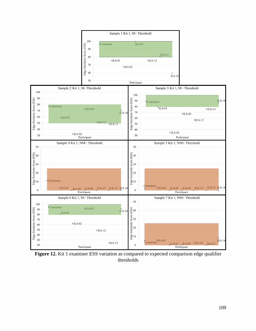
109
Figure 12. Kit 1 examiner ESS variation as compared to expected comparison edge qualifier
thresholds
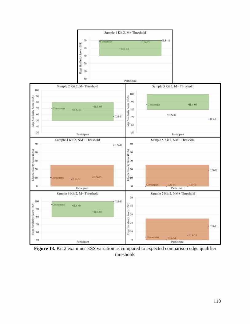
110
Figure 13. Kit 2 examiner ESS variation as compared to expected comparison edge qualifier
thresholds
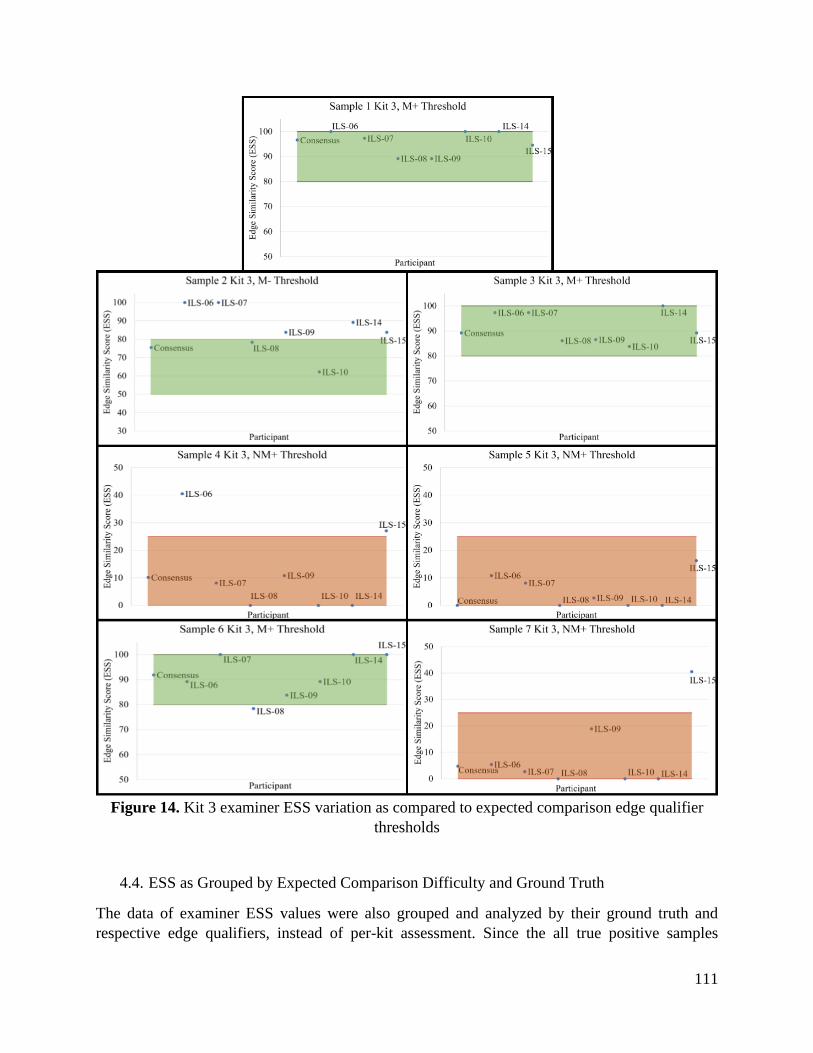
111
Figure 14. Kit 3 examiner ESS variation as compared to expected comparison edge qualifier
thresholds
4.4. ESS as Grouped by Expected Comparison Difficulty and Ground Truth
The data of examiner ESS values were also grouped and analyzed by their ground truth and
respective edge qualifiers, instead of per-kit assessment. Since the all true positive samples
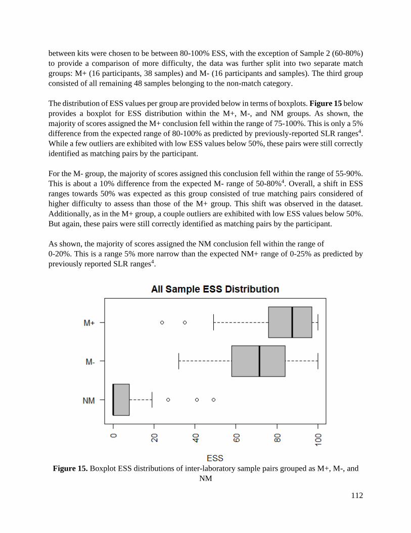
112
between kits were chosen to be between 80-100% ESS, with the exception of Sample 2 (60-80%)
to provide a comparison of more difficulty, the data was further split into two separate match
groups: M+ (16 participants, 38 samples) and M- (16 participants and samples). The third group
consisted of all remaining 48 samples belonging to the non-match category.
The distribution of ESS values per group are provided below in terms of boxplots. Figure 15 below
provides a boxplot for ESS distribution within the M+, M-, and NM groups. As shown, the
majority of scores assigned the M+ conclusion fell within the range of 75-100%. This is only a 5%
difference from the expected range of 80-100% as predicted by previously-reported SLR ranges4.
While a few outliers are exhibited with low ESS values below 50%, these pairs were still correctly
identified as matching pairs by the participant.
For the M- group, the majority of scores assigned this conclusion fell within the range of 55-90%.
This is about a 10% difference from the expected M- range of 50-80%4. Overall, a shift in ESS
ranges towards 50% was expected as this group consisted of true matching pairs considered of
higher difficulty to assess than those of the M+ group. This shift was observed in the dataset.
Additionally, as in the M+ group, a couple outliers are exhibited with low ESS values below 50%.
But again, these pairs were still correctly identified as matching pairs by the participant.
As shown, the majority of scores assigned the NM conclusion fell within the range of
0-20%. This is a range 5% more narrow than the expected NM+ range of 0-25% as predicted by
previously reported SLR ranges4.
Figure 15. Boxplot ESS distributions of inter-laboratory sample pairs grouped as M+, M-, and
NM
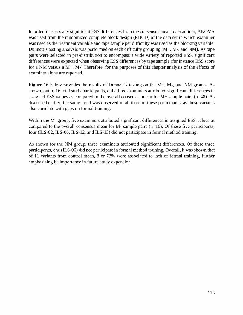
113
In order to assess any significant ESS differences from the consensus mean by examiner, ANOVA
was used from the randomized complete block design (RBCD) of the data set in which examiner
was used as the treatment variable and tape sample per difficulty was used as the blocking variable.
Dunnett’s testing analysis was performed on each difficulty grouping (M+, M-, and NM). As tape
pairs were selected in pre-distribution to encompass a wide variety of reported ESS, significant
differences were expected when observing ESS differences by tape sample (for instance ESS score
for a NM versus a M+, M-).Therefore, for the purposes of this chapter analysis of the effects of
examiner alone are reported.
Figure 16 below provides the results of Dunnett’s testing on the M+, M-, and NM groups. As
shown, out of 16 total study participants, only three examiners attributed significant differences in
assigned ESS values as compared to the overall consensus mean for M+ sample pairs (n=48). As
discussed earlier, the same trend was observed in all three of these participants, as these variants
also correlate with gaps on formal training.
Within the M- group, five examiners attributed significant differences in assigned ESS values as
compared to the overall consensus mean for M- sample pairs (n=16). Of these five participants,
four (ILS-02, ILS-06, ILS-12, and ILS-13) did not participate in formal method training.
As shown for the NM group, three examiners attributed significant differences. Of these three
participants, one (ILS-06) did not participate in formal method training. Overall, it was shown that
of 11 variants from control mean, 8 or 73% were associated to lack of formal training, further
emphasizing its importance in future study expansion.
114
Figure 16. Dunnett’s test examiner control differences results, M+, M-, and NM samples
115
4.5. Overall Observations
In summary, three general trends were observed. First, those participants that did not participate
in formal method training through either the in-person method presentation or teleconference
tended to exhibit statistically significant score differences from the consensus (N=4), pre-
distribution mean ESS. Some of those ESS differences, however, were not exclusionary when
using a broader threshold criterion (e.g. 20% ESS) or were not large enough to generate an
erroneous conclusion. As shown in Figure 16, out of 48 consensus mean comparisons (n=16
examiners per overall sample group – M+, M-, NM), only 11 instances (23%) showed significant
differences between mean reported ESS and consensus mean values, indicating a 77% agreement
with the pre-distribution, consensus mean. From those, only 8 out of 48 (17%) would provide a
misclassification of the qualifier (i.e. all significantly different NM ESS were still within the
expected range of a non-match, 0-50%). Also, from those remaining 8 differing results, 3 of them
were produced by analysts that did not elect to participate in formal method training beyond the
protocol and instructional presentation provided at the time of kit receipt. This indicates the
differences in reported values may be a result of lack of understanding of the proposed method.
Moreover, the differences on the remaining instances in which the participants did receive training
were not as drastic as to produce a false positive or false negative conclusion. For example, in two
of the three instances within the NM group that significant differences from the control mean arose,
both participants were present for formal training. In both situations, the examiners provided
overall non-match conclusions but ESS values of 40%. While the high ESS values as compared to
consensus means of ~5-11% resulted in significant statistical differences, neither instance resulted
in a misclassification. Higher scores were likely due to inconsistency in interpretation of scrim bin
features, as one examiner indicated even “featureless” bins were considered matching, leading to
an overall higher ESS despite the true negative conclusion.
Other main observations across the study included the variation in how a featureless scrim bin was
characterized for ESS purposes. This was made apparent through comments left by participants
per sample. While some chose to consider bins observed as featureless as matches (“1), others
chose to label them non-matches (“0”) due to the lack of edge features. Another key observation
included the various interpretations in the use of the comparison edge qualifier between
participants. These variances are best observed through ESS distributions by overall conclusion
and by assigned qualifier, respectively. These distributions are discussed below. It should be noted
that no matter the ESS variation, no misclassifications were made by the examiner of any samples
in any kits. A thorough evaluation of the potential sources of differences among reported ESS is
provided below.
4.5.1. ESS distributions by overall conclusion – variance in featureless/distorted bins
Figure 17 below provides the ESS distribution resulting from six participants completing Study
Kit 1. Scores of interest, referred to as “discrepancy instances” or “differences”, are numbered for
reference. It should be noted that other relatively low ESS values, such as the inconclusive of ESS
~ 25% and one of the true positives of ESS ~ 60% are not included in discussion as further
investigation into comments left by respective participants revealed that each felt multiple bins of
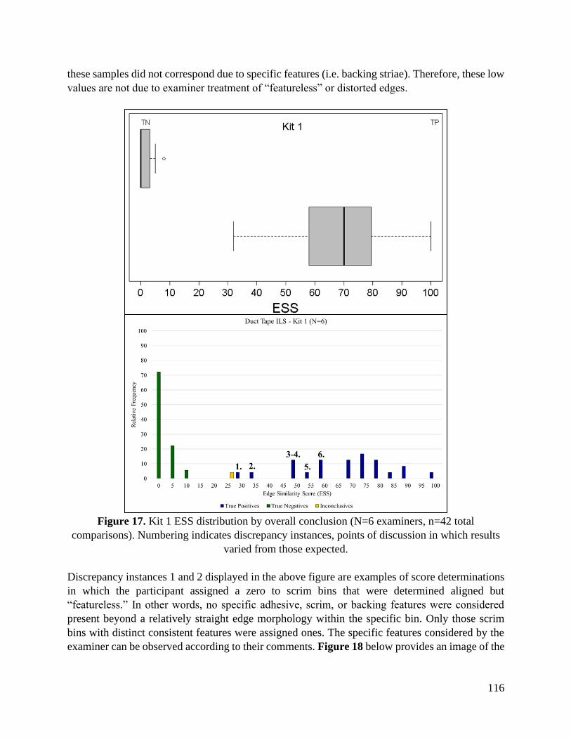
116
these samples did not correspond due to specific features (i.e. backing striae). Therefore, these low
values are not due to examiner treatment of “featureless” or distorted edges.
Figure 17. Kit 1 ESS distribution by overall conclusion (N=6 examiners, n=42 total
comparisons). Numbering indicates discrepancy instances, points of discussion in which results
varied from those expected.
Discrepancy instances 1 and 2 displayed in the above figure are examples of score determinations
in which the participant assigned a zero to scrim bins that were determined aligned but
“featureless.” In other words, no specific adhesive, scrim, or backing features were considered
present beyond a relatively straight edge morphology within the specific bin. Only those scrim
bins with distinct consistent features were assigned ones. The specific features considered by the
examiner can be observed according to their comments. Figure 18 below provides an image of the
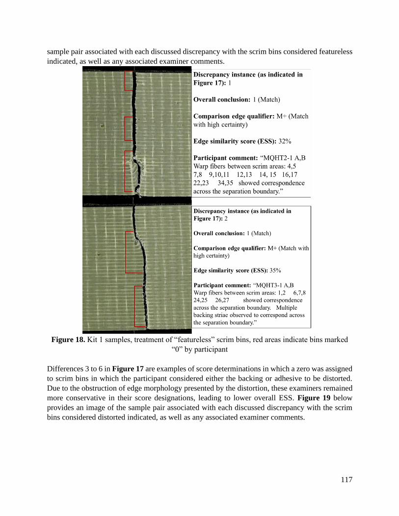
117
sample pair associated with each discussed discrepancy with the scrim bins considered featureless
indicated, as well as any associated examiner comments.
Figure 18. Kit 1 samples, treatment of “featureless” scrim bins, red areas indicate bins marked
“0” by participant
Differences 3 to 6 in Figure 17 are examples of score determinations in which a zero was assigned
to scrim bins in which the participant considered either the backing or adhesive to be distorted.
Due to the obstruction of edge morphology presented by the distortion, these examiners remained
more conservative in their score designations, leading to lower overall ESS. Figure 19 below
provides an image of the sample pair associated with each discussed discrepancy with the scrim
bins considered distorted indicated, as well as any associated examiner comments.
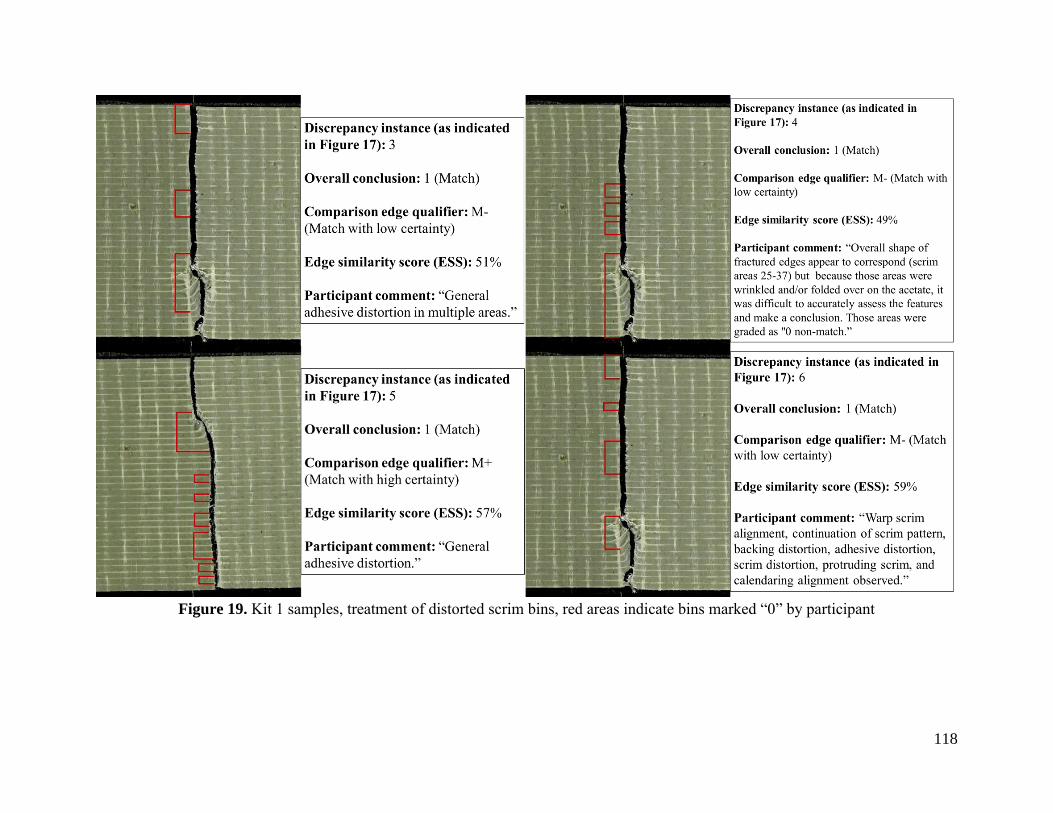
118
Figure 19. Kit 1 samples, treatment of distorted scrim bins, red areas indicate bins marked “0” by participant
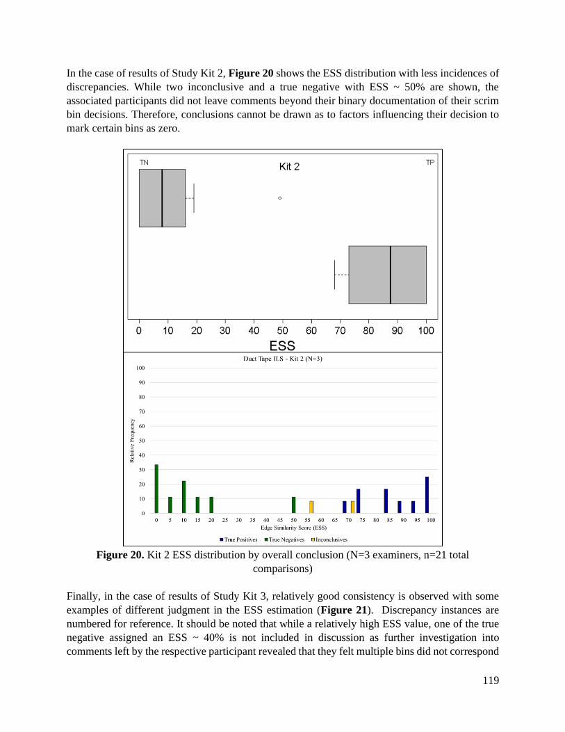
119
In the case of results of Study Kit 2, Figure 20 shows the ESS distribution with less incidences of
discrepancies. While two inconclusive and a true negative with ESS ~ 50% are shown, the
associated participants did not leave comments beyond their binary documentation of their scrim
bin decisions. Therefore, conclusions cannot be drawn as to factors influencing their decision to
mark certain bins as zero.
Figure 20. Kit 2 ESS distribution by overall conclusion (N=3 examiners, n=21 total
comparisons)
Finally, in the case of results of Study Kit 3, relatively good consistency is observed with some
examples of different judgment in the ESS estimation (Figure 21). Discrepancy instances are
numbered for reference. It should be noted that while a relatively high ESS value, one of the true
negative assigned an ESS ~ 40% is not included in discussion as further investigation into
comments left by the respective participant revealed that they felt multiple bins did not correspond
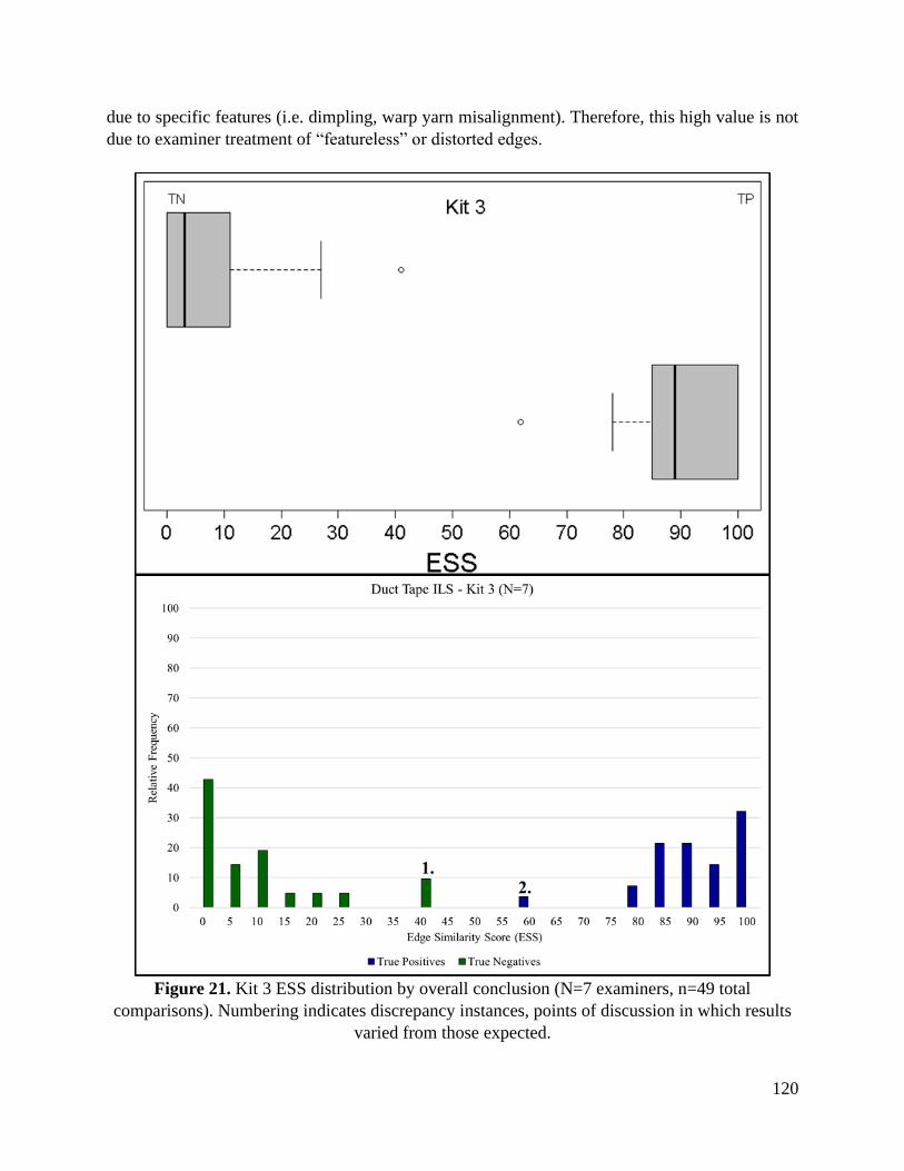
120
due to specific features (i.e. dimpling, warp yarn misalignment). Therefore, this high value is not
due to examiner treatment of “featureless” or distorted edges.
Figure 21. Kit 3 ESS distribution by overall conclusion (N=7 examiners, n=49 total
comparisons). Numbering indicates discrepancy instances, points of discussion in which results
varied from those expected.
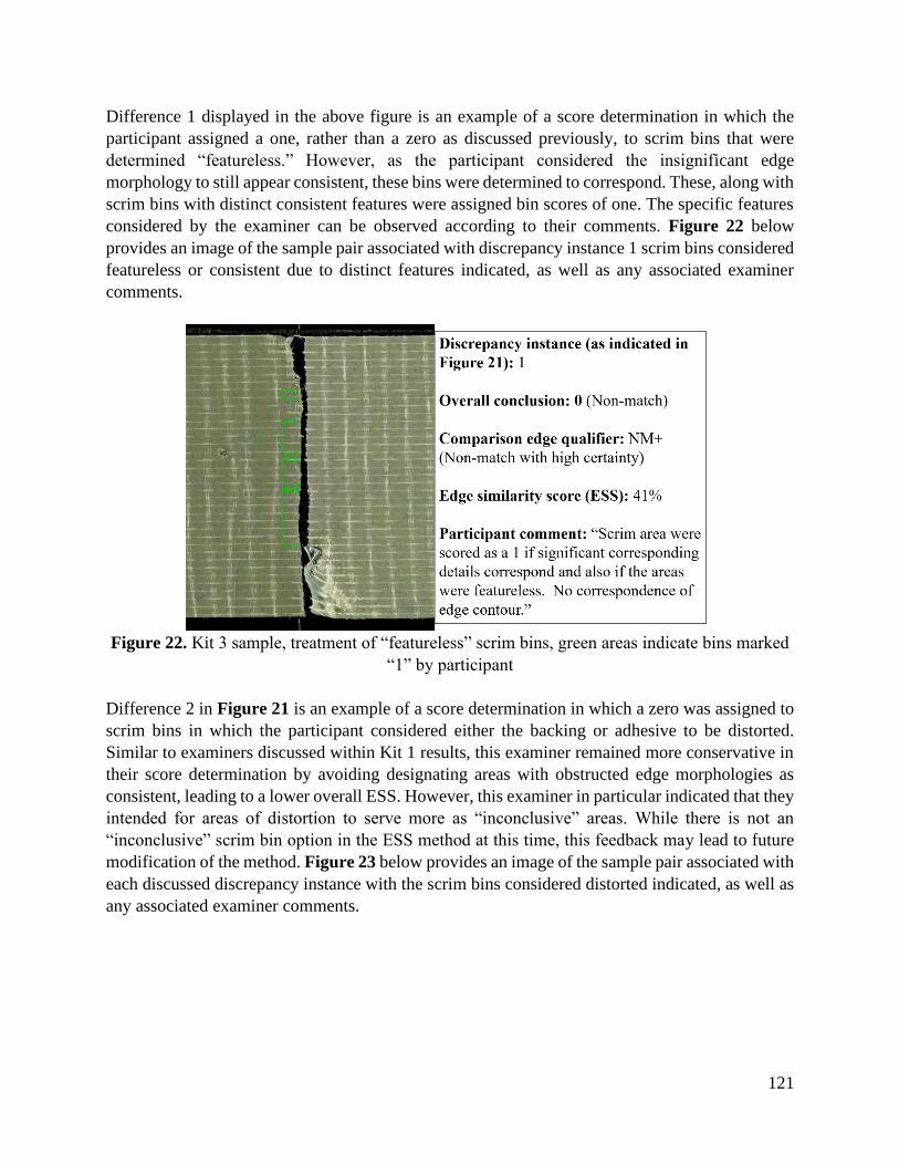
121
Difference 1 displayed in the above figure is an example of a score determination in which the
participant assigned a one, rather than a zero as discussed previously, to scrim bins that were
determined “featureless.” However, as the participant considered the insignificant edge
morphology to still appear consistent, these bins were determined to correspond. These, along with
scrim bins with distinct consistent features were assigned bin scores of one. The specific features
considered by the examiner can be observed according to their comments. Figure 22 below
provides an image of the sample pair associated with discrepancy instance 1 scrim bins considered
featureless or consistent due to distinct features indicated, as well as any associated examiner
comments.
Figure 22. Kit 3 sample, treatment of “featureless” scrim bins, green areas indicate bins marked
“1” by participant
Difference 2 in Figure 21 is an example of a score determination in which a zero was assigned to
scrim bins in which the participant considered either the backing or adhesive to be distorted.
Similar to examiners discussed within Kit 1 results, this examiner remained more conservative in
their score determination by avoiding designating areas with obstructed edge morphologies as
consistent, leading to a lower overall ESS. However, this examiner in particular indicated that they
intended for areas of distortion to serve more as “inconclusive” areas. While there is not an
“inconclusive” scrim bin option in the ESS method at this time, this feedback may lead to future
modification of the method. Figure 23 below provides an image of the sample pair associated with
each discussed discrepancy instance with the scrim bins considered distorted indicated, as well as
any associated examiner comments.
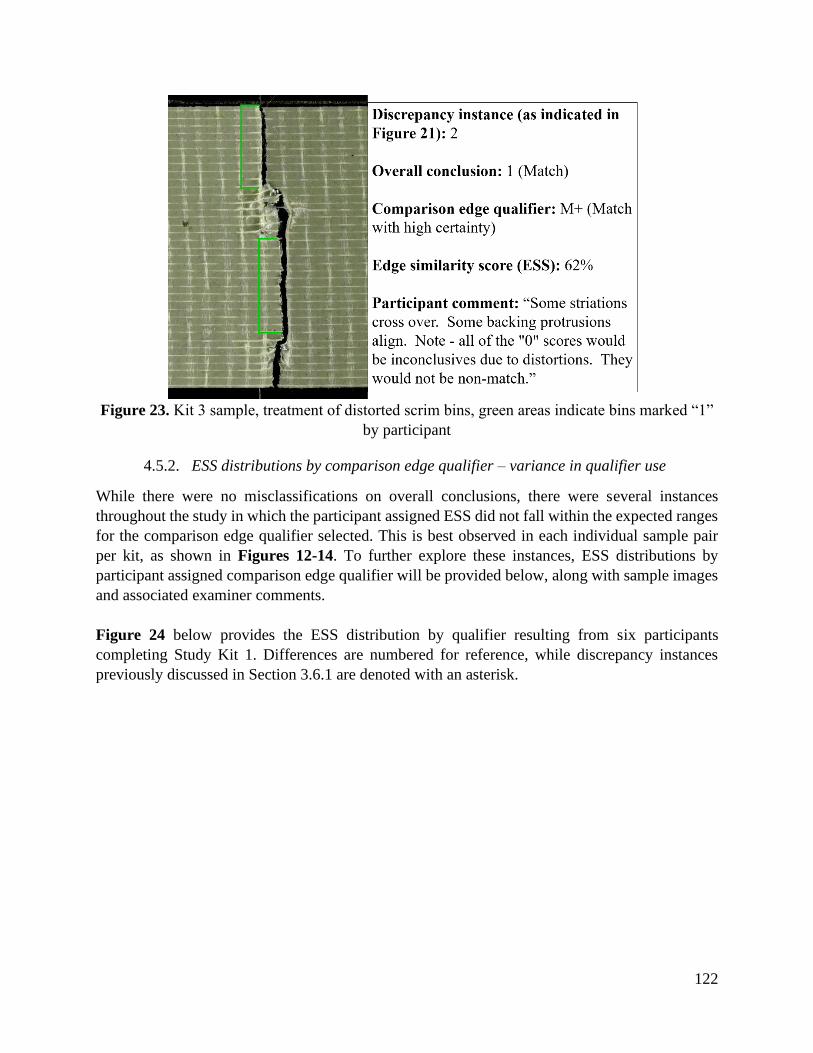
122
Figure 23. Kit 3 sample, treatment of distorted scrim bins, green areas indicate bins marked “1”
by participant
4.5.2. ESS distributions by comparison edge qualifier – variance in qualifier use
While there were no misclassifications on overall conclusions, there were several instances
throughout the study in which the participant assigned ESS did not fall within the expected ranges
for the comparison edge qualifier selected. This is best observed in each individual sample pair
per kit, as shown in Figures 12-14. To further explore these instances, ESS distributions by
participant assigned comparison edge qualifier will be provided below, along with sample images
and associated examiner comments.
Figure 24 below provides the ESS distribution by qualifier resulting from six participants
completing Study Kit 1. Differences are numbered for reference, while discrepancy instances
previously discussed in Section 3.6.1 are denoted with an asterisk.
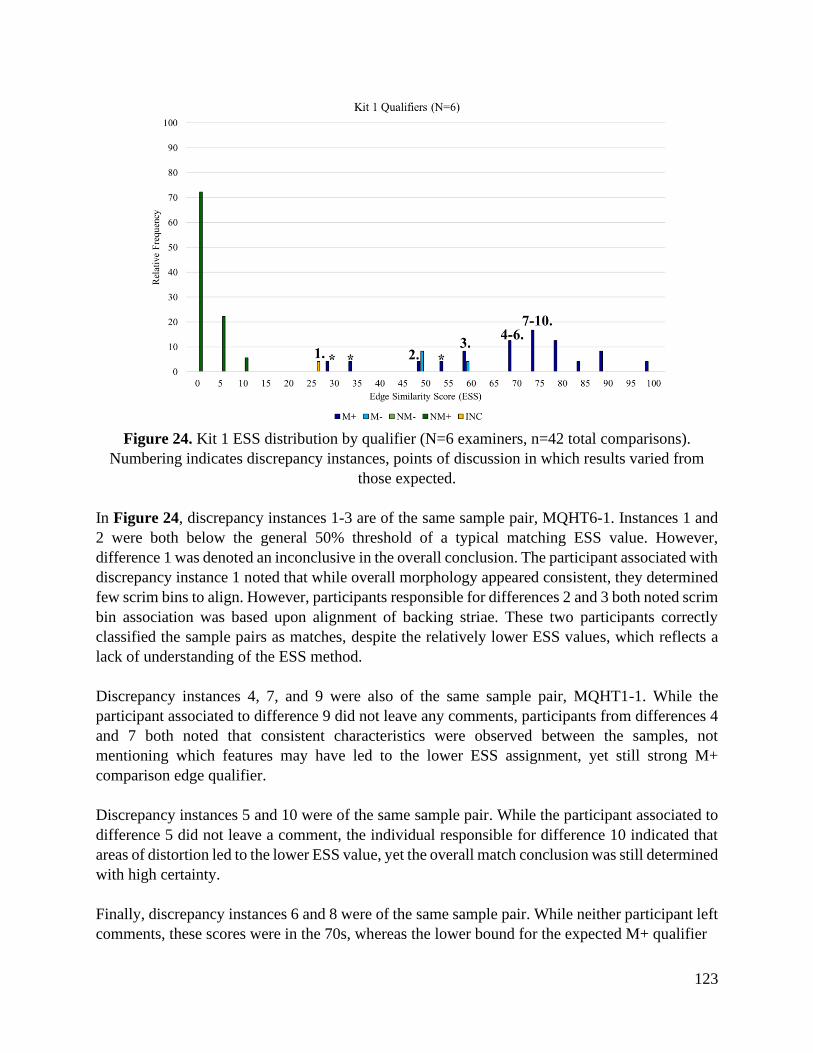
123
Figure 24. Kit 1 ESS distribution by qualifier (N=6 examiners, n=42 total comparisons).
Numbering indicates discrepancy instances, points of discussion in which results varied from
those expected.
In Figure 24, discrepancy instances 1-3 are of the same sample pair, MQHT6-1. Instances 1 and
2 were both below the general 50% threshold of a typical matching ESS value. However,
difference 1 was denoted an inconclusive in the overall conclusion. The participant associated with
discrepancy instance 1 noted that while overall morphology appeared consistent, they determined
few scrim bins to align. However, participants responsible for differences 2 and 3 both noted scrim
bin association was based upon alignment of backing striae. These two participants correctly
classified the sample pairs as matches, despite the relatively lower ESS values, which reflects a
lack of understanding of the ESS method.
Discrepancy instances 4, 7, and 9 were also of the same sample pair, MQHT1-1. While the
participant associated to difference 9 did not leave any comments, participants from differences 4
and 7 both noted that consistent characteristics were observed between the samples, not
mentioning which features may have led to the lower ESS assignment, yet still strong M+
comparison edge qualifier.
Discrepancy instances 5 and 10 were of the same sample pair. While the participant associated to
difference 5 did not leave a comment, the individual responsible for difference 10 indicated that
areas of distortion led to the lower ESS value, yet the overall match conclusion was still determined
with high certainty.
Finally, discrepancy instances 6 and 8 were of the same sample pair. While neither participant left
comments, these scores were in the 70s, whereas the lower bound for the expected M+ qualifier
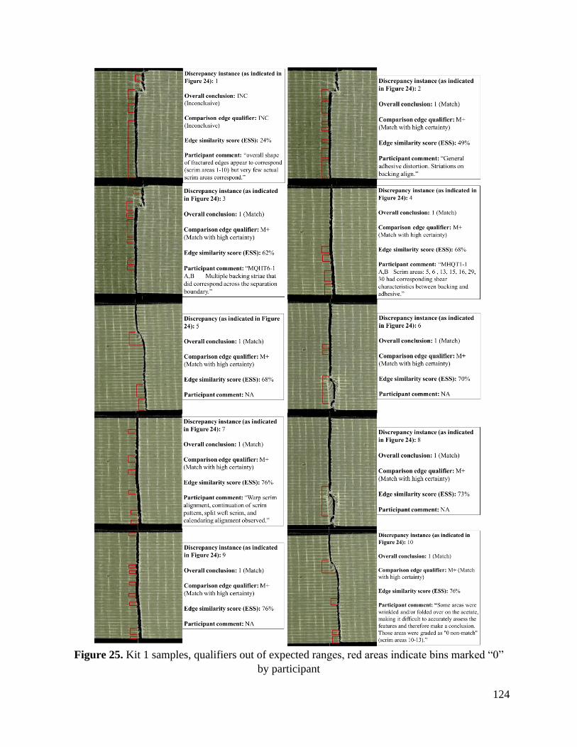
124
Figure 25. Kit 1 samples, qualifiers out of expected ranges, red areas indicate bins marked “0”
by participant
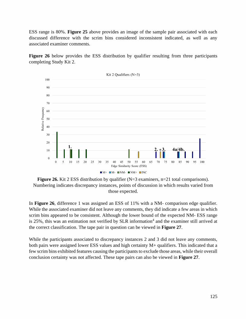
125
ESS range is 80%. Figure 25 above provides an image of the sample pair associated with each
discussed difference with the scrim bins considered inconsistent indicated, as well as any
associated examiner comments.
Figure 26 below provides the ESS distribution by qualifier resulting from three participants
completing Study Kit 2.
Figure 26. Kit 2 ESS distribution by qualifier (N=3 examiners, n=21 total comparisons).
Numbering indicates discrepancy instances, points of discussion in which results varied from
those expected.
In Figure 26, difference 1 was assigned an ESS of 11% with a NM- comparison edge qualifier.
While the associated examiner did not leave any comments, they did indicate a few areas in which
scrim bins appeared to be consistent. Although the lower bound of the expected NM- ESS range
is 25%, this was an estimation not verified by SLR information4 and the examiner still arrived at
the correct classification. The tape pair in question can be viewed in Figure 27.
While the participants associated to discrepancy instances 2 and 3 did not leave any comments,
both pairs were assigned lower ESS values and high certainty M+ qualifiers. This indicated that a
few scrim bins exhibited features causing the participants to exclude those areas, while their overall
conclusion certainty was not affected. These tape pairs can also be viewed in Figure 27.
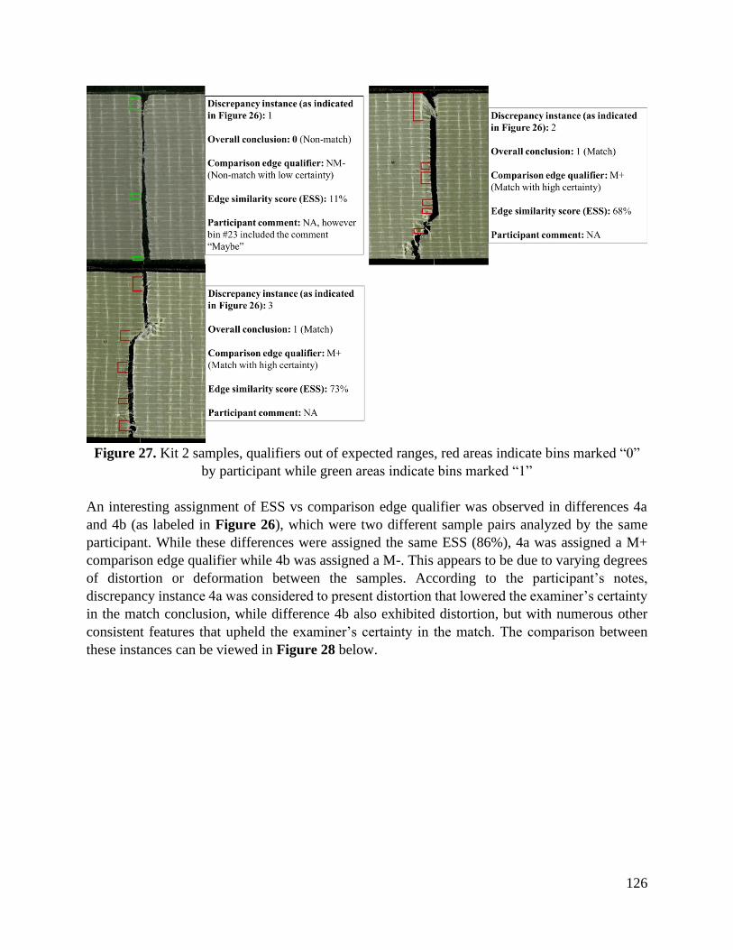
126
Figure 27. Kit 2 samples, qualifiers out of expected ranges, red areas indicate bins marked “0”
by participant while green areas indicate bins marked “1”
An interesting assignment of ESS vs comparison edge qualifier was observed in differences 4a
and 4b (as labeled in Figure 26), which were two different sample pairs analyzed by the same
participant. While these differences were assigned the same ESS (86%), 4a was assigned a M+
comparison edge qualifier while 4b was assigned a M-. This appears to be due to varying degrees
of distortion or deformation between the samples. According to the participant’s notes,
discrepancy instance 4a was considered to present distortion that lowered the examiner’s certainty
in the match conclusion, while difference 4b also exhibited distortion, but with numerous other
consistent features that upheld the examiner’s certainty in the match. The comparison between
these instances can be viewed in Figure 28 below.
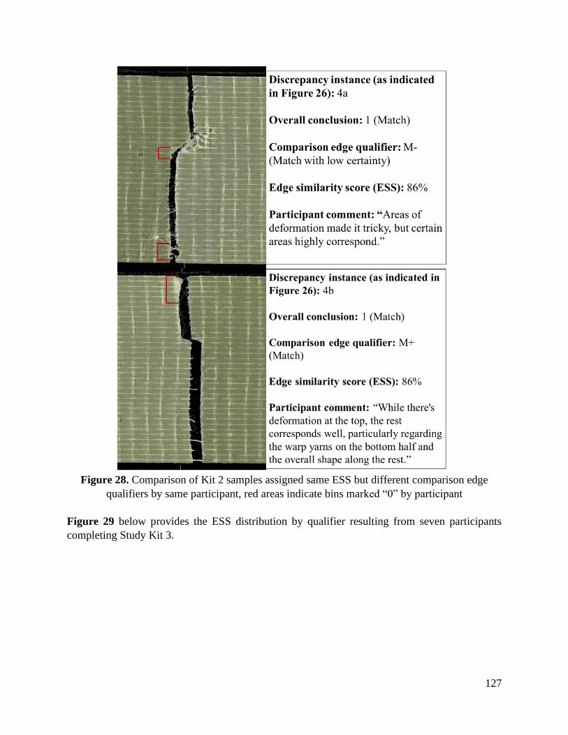
127
Figure 28. Comparison of Kit 2 samples assigned same ESS but different comparison edge
qualifiers by same participant, red areas indicate bins marked “0” by participant
Figure 29 below provides the ESS distribution by qualifier resulting from seven participants
completing Study Kit 3.
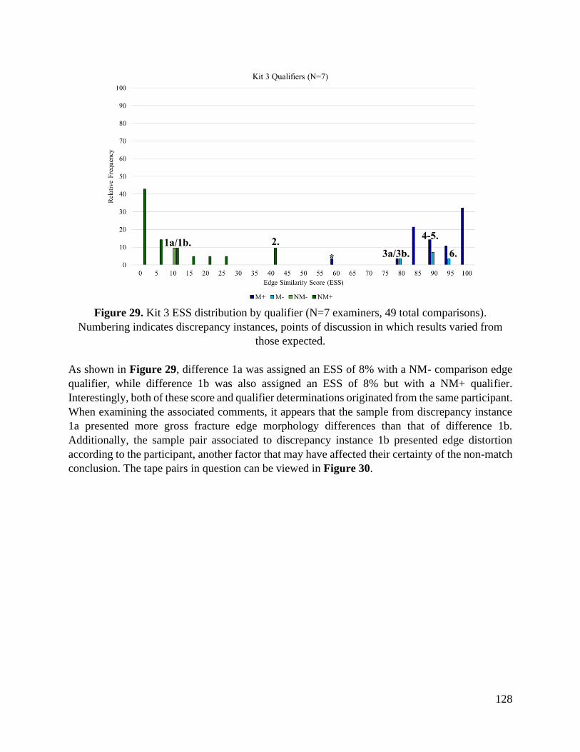
128
Figure 29. Kit 3 ESS distribution by qualifier (N=7 examiners, 49 total comparisons).
Numbering indicates discrepancy instances, points of discussion in which results varied from
those expected.
As shown in Figure 29, difference 1a was assigned an ESS of 8% with a NM- comparison edge
qualifier, while difference 1b was also assigned an ESS of 8% but with a NM+ qualifier.
Interestingly, both of these score and qualifier determinations originated from the same participant.
When examining the associated comments, it appears that the sample from discrepancy instance
1a presented more gross fracture edge morphology differences than that of difference 1b.
Additionally, the sample pair associated to discrepancy instance 1b presented edge distortion
according to the participant, another factor that may have affected their certainty of the non-match
conclusion. The tape pairs in question can be viewed in Figure 30.
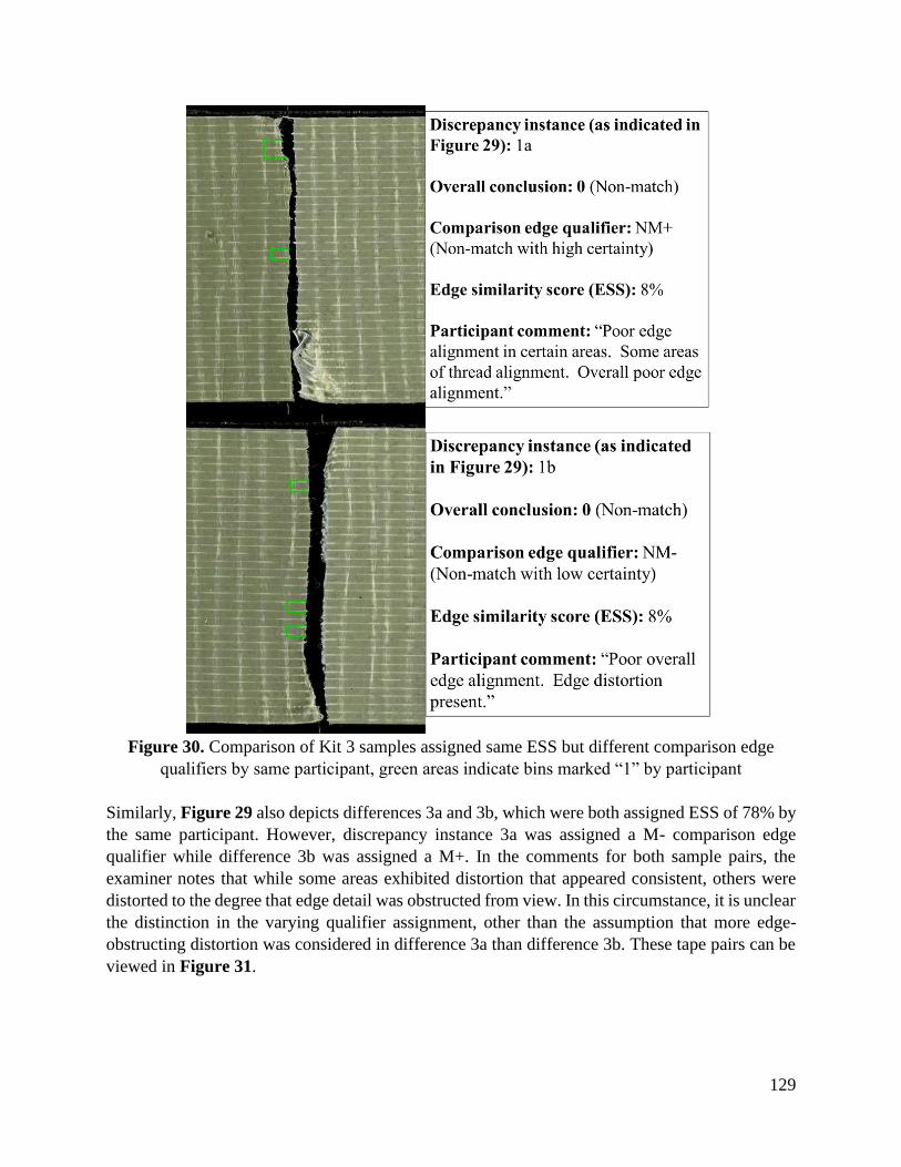
129
Figure 30. Comparison of Kit 3 samples assigned same ESS but different comparison edge
qualifiers by same participant, green areas indicate bins marked “1” by participant
Similarly, Figure 29 also depicts differences 3a and 3b, which were both assigned ESS of 78% by
the same participant. However, discrepancy instance 3a was assigned a M- comparison edge
qualifier while difference 3b was assigned a M+. In the comments for both sample pairs, the
examiner notes that while some areas exhibited distortion that appeared consistent, others were
distorted to the degree that edge detail was obstructed from view. In this circumstance, it is unclear
the distinction in the varying qualifier assignment, other than the assumption that more edge-
obstructing distortion was considered in difference 3a than difference 3b. These tape pairs can be
viewed in Figure 31.
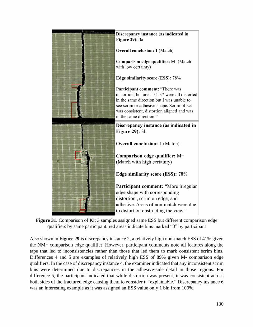
130
Figure 31. Comparison of Kit 3 samples assigned same ESS but different comparison edge
qualifiers by same participant, red areas indicate bins marked “0” by participant
Also shown in Figure 29 is discrepancy instance 2, a relatively high non-match ESS of 41% given
the NM+ comparison edge qualifier. However, participant comments note all features along the
tape that led to inconsistencies rather than those that led them to mark consistent scrim bins.
Differences 4 and 5 are examples of relatively high ESS of 89% given M- comparison edge
qualifiers. In the case of discrepancy instance 4, the examiner indicated that any inconsistent scrim
bins were determined due to discrepancies in the adhesive-side detail in those regions. For
difference 5, the participant indicated that while distortion was present, it was consistent across
both sides of the fractured edge causing them to consider it “explainable.” Discrepancy instance 6
was an interesting example as it was assigned an ESS value only 1 bin from 100%.
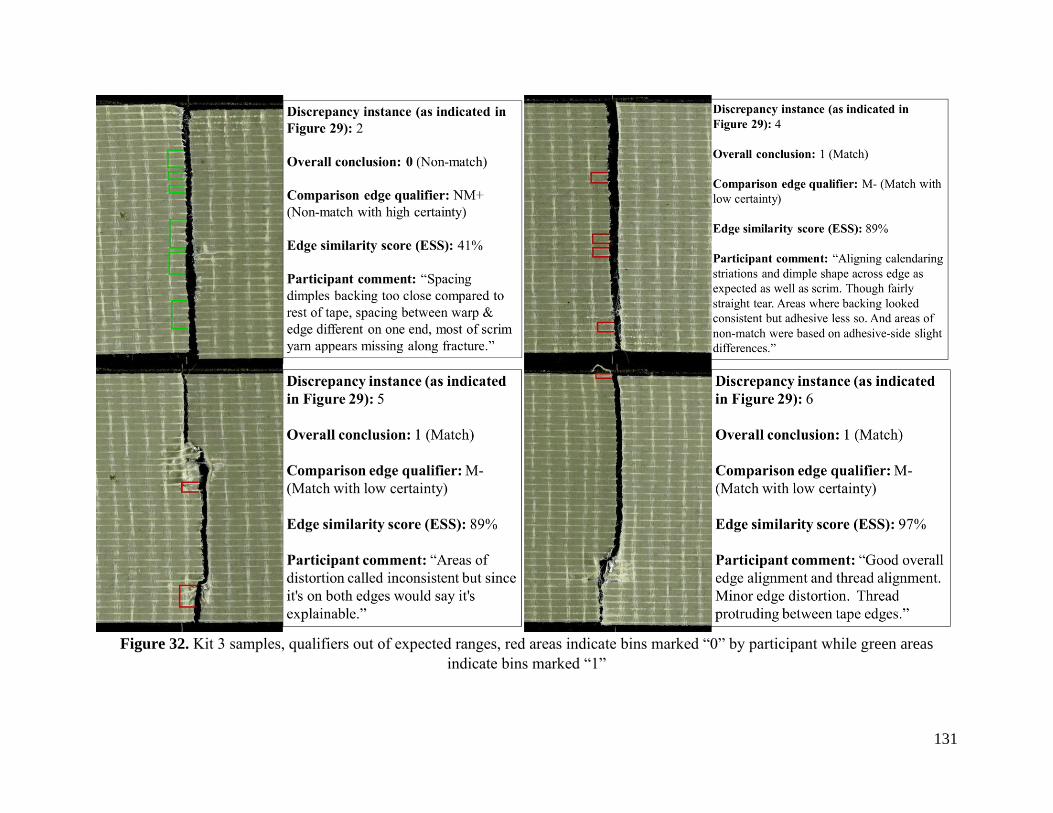
131
Figure 32. Kit 3 samples, qualifiers out of expected ranges, red areas indicate bins marked “0” by participant while green areas
indicate bins marked “1”
132
One bin was marked “0” due to a protruding yarn that was determined to be inconsistent with the
corresponding edge. The examiner does denote that minor edge distortion was observed in addition
to the protruding yarn, perhaps causing them to assign a qualifier of lower certainty. Images of
these samples are provided in Figure 32 above.
In summary, a more in-depth assessment of the potential sources of dissimilarities between
examiners’ results and deviations from the consensus ESS scores was conducted by evaluating the
comments each examiner documented on the ESS bin comparison sheets. Also, the respective tape
images were carefully studied to identify which areas need further training to improve inter-
examiner agreement and to use the ESS method to its full potential. These types of assessments
would not have been possible without the systematic analysis and documentation approach
developed in this ILS. The bin-to-bin scores and corresponding notes, allowed us to do a thorough
comparison of observed features and opinions between examiners, illustrating the utility of the
ESS method for peer review process.
Specifically, the bin-to-bin evaluation revealed that the interpretation of the distinctiveness of
features varied between some examiners. Less distinctive characteristics within a bin area, such as
“featureless” straight edges or distorted edges were the most problematic. This feedback may
indicate the need for a weighting factor to be applied to the method, in addition to the ESS, in order
for examiners to best demonstrate a scrim bin that is consistent due to prominent physical features
(e.g. corresponding protruding scrim or backing striae) versus a less distinctive scrim bin.
4.5.3. Agreement of inter-laboratory ESS values and observed distributions in matched
and non-matched pairs of larger datasets
Despite any interpretation variances at the micro-level, the majority of overall ESS reported by
participants were within approximate ±20% ranges as compared to pre-distribution, consensus
values with the exception of 15 out of 112 comparisons (N=16 examiners overall, n=112 total
comparisons). When considering examiner overall conclusion despite assigned ESS value, no
misclassifications were observed throughout the study. When considering classification by the
expected 50/50 ESS threshold, overall error rates were as follows: 92% true positives (59/64), 8%
false negatives (5/64), 100% true negatives (48/48), and 0% false positives (0/48). Moreover,
overall agreement between examiners is shown in the boxplot distributions by ESS, provided in
Figure 33 below. Additionally, as shown in Figure 34, overall study ESS distribution was similar
to that of the true positives and true negatives of the larger population study,4 in which scores
>80% supported M+ and scores <25% supported NM.
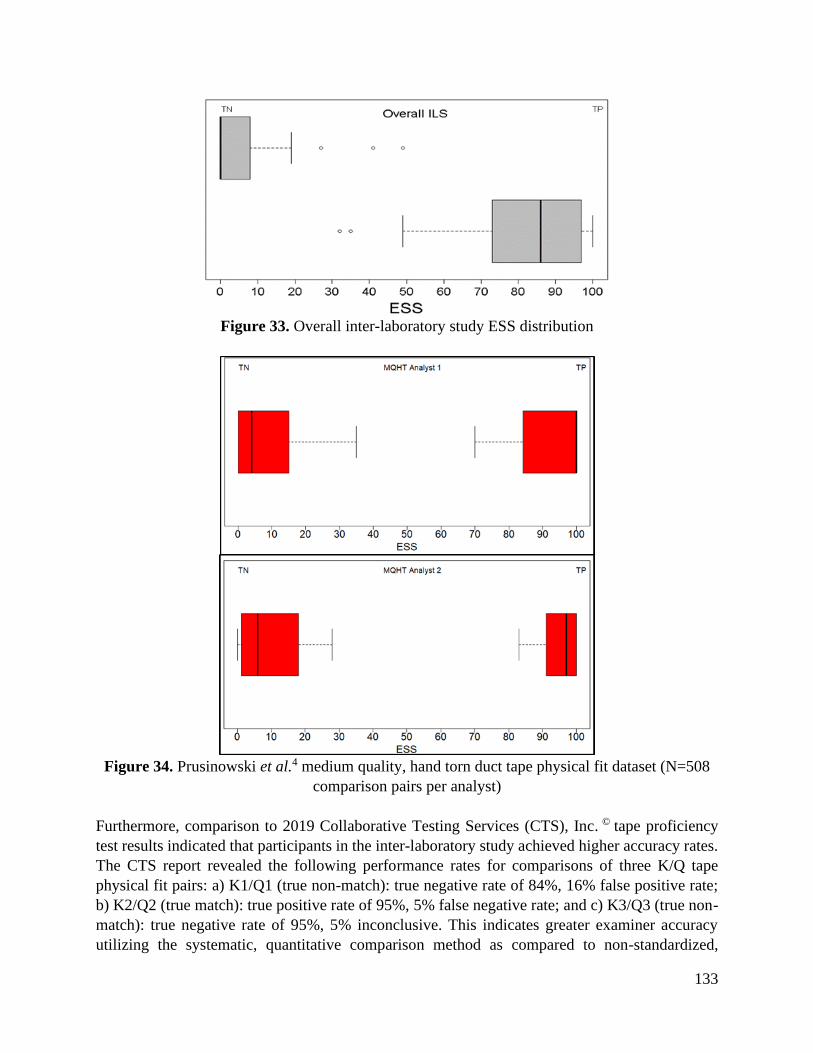
133
Figure 33. Overall inter-laboratory study ESS distribution
Figure 34. Prusinowski et al.4 medium quality, hand torn duct tape physical fit dataset (N=508
comparison pairs per analyst)
Furthermore, comparison to 2019 Collaborative Testing Services (CTS), Inc. © tape proficiency
test results indicated that participants in the inter-laboratory study achieved higher accuracy rates.
The CTS report revealed the following performance rates for comparisons of three K/Q tape
physical fit pairs: a) K1/Q1 (true non-match): true negative rate of 84%, 16% false positive rate;
b) K2/Q2 (true match): true positive rate of 95%, 5% false negative rate; and c) K3/Q3 (true non-
match): true negative rate of 95%, 5% inconclusive. This indicates greater examiner accuracy
utilizing the systematic, quantitative comparison method as compared to non-standardized,
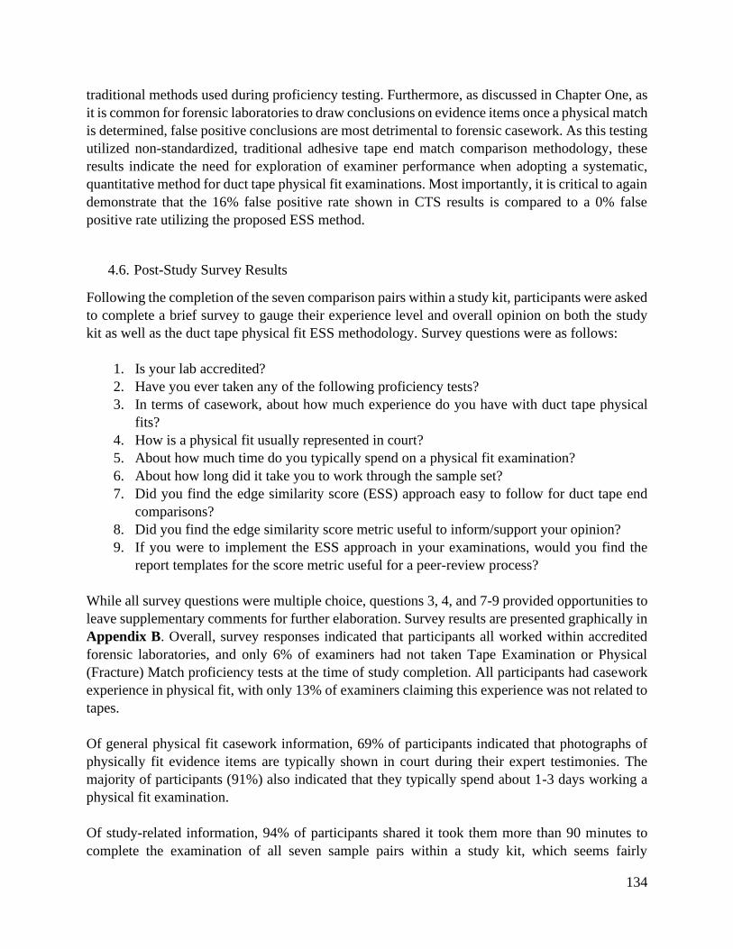
134
traditional methods used during proficiency testing. Furthermore, as discussed in Chapter One, as
it is common for forensic laboratories to draw conclusions on evidence items once a physical match
is determined, false positive conclusions are most detrimental to forensic casework. As this testing
utilized non-standardized, traditional adhesive tape end match comparison methodology, these
results indicate the need for exploration of examiner performance when adopting a systematic,
quantitative method for duct tape physical fit examinations. Most importantly, it is critical to again
demonstrate that the 16% false positive rate shown in CTS results is compared to a 0% false
positive rate utilizing the proposed ESS method.
4.6. Post-Study Survey Results
Following the completion of the seven comparison pairs within a study kit, participants were asked
to complete a brief survey to gauge their experience level and overall opinion on both the study
kit as well as the duct tape physical fit ESS methodology. Survey questions were as follows:
1. Is your lab accredited?
2. Have you ever taken any of the following proficiency tests?
3. In terms of casework, about how much experience do you have with duct tape physical
fits?
4. How is a physical fit usually represented in court?
5. About how much time do you typically spend on a physical fit examination?
6. About how long did it take you to work through the sample set?
7. Did you find the edge similarity score (ESS) approach easy to follow for duct tape end
comparisons?
8. Did you find the edge similarity score metric useful to inform/support your opinion?
9. If you were to implement the ESS approach in your examinations, would you find the
report templates for the score metric useful for a peer-review process?
While all survey questions were multiple choice, questions 3, 4, and 7-9 provided opportunities to
leave supplementary comments for further elaboration. Survey results are presented graphically in
Appendix B. Overall, survey responses indicated that participants all worked within accredited
forensic laboratories, and only 6% of examiners had not taken Tape Examination or Physical
(Fracture) Match proficiency tests at the time of study completion. All participants had casework
experience in physical fit, with only 13% of examiners claiming this experience was not related to
tapes.
Of general physical fit casework information, 69% of participants indicated that photographs of
physically fit evidence items are typically shown in court during their expert testimonies. The
majority of participants (91%) also indicated that they typically spend about 1-3 days working a
physical fit examination.
Of study-related information, 94% of participants shared it took them more than 90 minutes to
complete the examination of all seven sample pairs within a study kit, which seems fairly
135
reasonable. The majority of participants also found the ESS approach average to easy in difficulty,
indicating promise for smooth incorporation to current practice.
As far as examiner opinion, participants were split in their feelings of the assessment of usefulness
of the ESS approach. Half of participants indicated the approach was not useful, with most of the
comments revealed lack of understanding of the purpose of the ESS method or resistance to
change, which is expected in the assessment of new approaches that differ from conventional
protocols. As a result, we believe these negative perceptions are easy to correct in the future with
further training and more detailed explanation of the scope and capabilities of the proposed
approach. For instance, some of the expressed concerns were: 1) that the ESS would diminish the
significance of a physical fit in the eyes of a jury if it is not 100%, 2) that the examiner felt he/she
had a bias in determining ESS due to their prior opinion of whether or not there was a match before
estimating the ESS, and 3) that they did not feel their overall opinion should be based on a score.
As seen, these concerns, are easy to overcome with further training and communication with the
end-users. For example, during a follow-up meeting with participants to discuss the ILS results,
we stressed the ESS method is not intended to be the sole step on a physical match examination
but rather a means to support and inform the examiner opinion. We also discussed the relevance
of recognizing that not every match holds the same weight, and that a 100% perfect match is not
always plausible, as demonstrated by our data. The ILS also demonstrated that as in any other
discipline, it is impossible to be error-free. However, what is critical is we can identify and report
sources of error and uncertainty. In addition, we noted that 63% of examiners that indicated “not
useful” within the post-study survey did not receive the formal training and method interpretation
discussion that allowed the researchers to be more familiar and open-minded with the proposed
methodology.
On the other hand, the majority (81%) of participants did feel that the ESS method and the scrim
bin reporting templates would be useful tools for technical review of case reports and training of
examiners. Indeed, the ESS method provides for the first time an opportunity for a blind,
systematic, and transparent peer review process.
These comments are valuable as they draw to the researcher’s attention the aspects of hesitation
that some practitioners would demonstrate upon a decision to implement this methodology in their
respective laboratories. As is common in this type of interlaboratory studies, the practitioners’
feedback provided an opportunity to fine-tune the ESS method and most importantly, modify the
training strategies to increase reproducibility in ESS between examiners and discuss crucial points
of ESS interpretation. Therefore, this study provided the baseline from which future work may
grow.
136
5. Conclusions and Future Work
The purpose of this project was to develop and implement an inter-laboratory study in order to
evaluate the performance of the proposed score-based method in assessing a potential duct tape
physical fit. Of particular interest in this pilot study was the assessment of inter-examiner
agreement, examiner error rates, and feedback from participants to facilitate the future adoption of
the method to their laboratories. This study utilized the ESS methodology previously developed
by Prusinowski et al.4 Three study kits were developed with sixteen forensic practitioner
participants overall and ESS and conclusions reported for 112 duct tape fractured paired samples.
Overall, inter-examiner agreement with reporting ESS scores within 20% of the mean consensus
values was observed. The participants' accuracy ranged from 88 to 100%, depending on the quality
of the match and test kit. Moreover, the inter-laboratory study highlighted the utility of the ESS
score method to enhance future physical fit practice in several aspects:
a) Increased objectivity: Although human judgment will always be needed for physical fit
examinations, the use of subjective decisions is risky when used without standardized criteria. The
ESS score method allows, for the first time, established thresholds and standards that can be used
for informing and supporting the examiners' opinion regarding the quality of a match.
b) Consensus: one of the challenges faced by forensic practitioners is to identify when a
physical fit presents enough distinctive characteristics to decide between a match, a good match,
an inconclusive, or a non-match conclusion. The ESS score has shown promise towards
standardization of criteria and systematic documentation and peer review process. Most
importantly, the reproducible bin-to-bin comparison of features leaves room for future
improvement on the estimation of occurrence of rare or distinctive micro-features. Inter-laboratory
studies using the ESS would help us in the near future identify which areas and features hold more
weight during an examination and how and why we can arrive at consensus protocols.
c) Scientific reliability: the ESS scores and the ILS studies allow for estimation of
performance rates, false positives, false negatives, overall accuracy, and inter-examiner agreement.
Also, it provides a means to estimate which factors can affect the uncertainty of a physical fit. All
of those measures provide a valuable empirically demonstrable basis to assess the significance of
a fit.
A careful evaluation of the data, the bin-to-bin examiners' documentation, and the survey's
feedback revealed three main observations across result sets. First, those participants that did not
participate in formal method training through either the in-person method presentation or
teleconference tended to exhibit statistically significant score differences from the consensus, pre-
distribution mean ESS. This was shown through results of the Dunnett’s test as well as distribution
of scores. Of the 33% of participants presenting larger deviations with the consensus mean, 73%
did not elect to participate in formal method training beyond the protocol and instructional
presentation provided at the time of kit receipt. On the other hand, the majority of examiners who
137
were exposed to formal instruction demonstrated agreement with consensus values and with
distribution of score thresholds as compared with larger population datasets. As a result, future
ILS would include more in-depth mandatory training as a pre-requisite to participation.
Other main observations across the study included variance in which examiners treated and
interpreted a featureless or distorted region of scrim bins for ESS purposes. While some examiners
assigned a binary classifier of 0 to these areas (non-matching, inconsistent bin determinations),
others felt these areas could still be determined consistent and assigned a binary classifier of 1 to
these areas (matching, consistent bin determinations). Further, some examiners noted that the
method may be more beneficial with an inconclusive variable option or a weighing factor for scrim
bins instead of just binary output (1 or 0). Those recommendations are currently being incorporated
for future tests.
It was also determined that more training is needed to aid examiners with the interpretations in the
use of the comparison edge qualifier. While expected ranges were set for ESS based on the
assignment of comparison edge qualifiers according to previously determined score likelihood
ratios (SLRs)4, many examiners did not provided qualifiers that were reasonable for certain ESS
ranges.
Despite slight interpretation variation, the majority of ESS reported by participants were
within approximate ±20% ranges as compared to pre-distribution, consensus values with
the exception of 15 out of 112 instances (N=16 examiners overall, n=112 total
comparisons). No misclassifications were observed throughout the study by overall examiner
conclusion per comparison pair. Observed error rates were as follows: 95% true positives (61/64),
0% false negatives (0/48), 100% true negatives (48/48), and 0% false positives (0/64). The
reduction in the true positive rate is the result of a 5% inconclusive rate (3 true positive samples
were concluded as inconclusive across the sample set). When considering classification by the
expected 50/50 non-match/match ESS threshold, overall error rates were as follows: 92% true
positives (59/64), 8% false negatives (5/48), 100% true negatives (48/48), and 0% false positives
(0/64).
Future work will include modification of the ESS method based upon examiner feedback received
during the post-study survey to expand the binary outputs on the ESS scores and include further
guidelines on macro assessments. Following optimization, expanded distribution of the inter-
laboratory study will be initiated in order to further validate the methodology for potential
implementation into forensic laboratories. Utilization of the ESS method in duct tape physical fit
examinations will uphold the high level of association offered by physical fits while reducing
subjectivity and creating a more transparent review and interpretation process.
Future work will also include expanding upon a preliminary, linear mixed model fit by restricted
maximum likelihood (REML) applied to the inter-laboratory ESS data in order to further assess
the amount of variance existing between participant results. Within the model, sample groups by
anticipated level of difficulty (expected comparison edge qualifier and ground truth) were utilized
as the fixed effect. This resulted in three levels by sample group: easy true match (M+), difficult
138
true match (M-), and true non-match (NM). The random effects on ESS results were described by
two factors: the different sample groups by difficulty (3 levels) and the examiners participating in
the study. In this manner, variance of study participants was able to be observed while correcting
for the fact that different examiners were viewing different physical samples between the 3 kits.
Application of the model to the current dataset revealed that variance between examiners was less
than between different kits. However, this model is still in progress. As the current model does not
apply significance testing and is descriptive of score variation alone, eventual expansion seeks to
apply a Bayesian model to provide credible intervals for variation between examiners. In addition,
fit of the model is expected to improve with a greater input of ESS data due to increased
participants in future expanded distribution of the study kits.
The results from this ILS demonstrated that the proposed ESS method can provide support to
examiner conclusions, offer systematic criteria that can lead to consensus-based methods, and
allow for a quantitative assessment of factors influencing the quality of a fit as well as estimation
of inter-examiner error rates. Examiners also recognized the method provides an avenue to conduct
a systematic and transparent peer-review process, which is otherwise not possible with current
examination protocols.
6. References
1. National Academy of Sciences (NAS). Strengthening Forensic Science in the United States: A
Path Forward. 2009. doi:0.17226/12589
2. President’s Council of Advisors on Science and Technology. Forensic Science in Criminal
Courts: Ensuring Scientific Validity of Feature-Comparison Methods. 2016.
3. American Statistical Association. American Statistical Association Position on Statistical
Statements for Forensic Evidence. [accessed 2019 Jan 30].
https://www.amstat.org/asa/files/pdfs/POL-ForensicScience.pdf
4. Prusinowski M, Brooks E, Trejos T. Development and validation of a systematic approach for
the quantitative assessment of the quality of duct tape physical fits. Forensic Science International.
2020;307.
5. Bradley MJ, Keagy RL, Lowe PC, Rickenbach MP, Wright DM, LeBeau MA. A validation
study for duct tape end matches. Journal of Forensic Sciences. 2006;51(3):504–508.
doi:10.1111/j.1556-4029.2006.00106.x
6. McCabe KR, Tulleners FA, Braun J V, Currie G, Gorecho EN. A Quantitative Analysis of Torn
and Cut Duct Tape Physical End Matching. Journal of Forensic Sciences. 2013;58(S1):S34–S42.
7. ISO/IEC 17043:2010 Conformity assessment - General requirements for proficiency testing.
2010.
8. Ivanov AR, Colangelo CM, Dufresne CP, Friedman DB, Lilley KS, Mechtler K, Phinney BS,
Rose KL, Rudnick PA, Searle BC, et al. Interlaboratory studies and initiatives developing
standards for proteomics. Proteomics. 2013;13(6):904–909. doi:10.1002/pmic.201200532
139
9. International Study Group. An inter-laboratory comparison of radiocarbon measurements in tree
rings. Nature. 1982;298:619–623. doi:10.1038/298619a0
10. Chung JH, Cho K, Kim S, Jeon SH, Shin JH, Lee J, Ahn YG. Inter-Laboratory Validation of
Method to Determine Residual Enrofloxacin in Chicken Meat. International Journal of Analytical
Chemistry. 2018;2018. doi:10.1155/2018/6019549
11. Hoffman T, Corzo R, Weis P, Pollock E, van Es A, Wiarda W, Stryjnik A, Dorn H, Heydon
A, Hoise E, et al. An inter-laboratory evaluation of LA-ICP-MS analysis of glass and the use of a
database for the interpretation of glass evidence. Forensic Chemistry. 2018;11:65–76.
doi:10.1016/j.forc.2018.10.001
12. Lucidarme D, Decoster A, Delamare C, Schmitt C, Kozlowski D, Harbonnier J, Jacob C, Cyran
C, Forzy G, Defer C, et al. An inter-laboratory study of anti-HCV antibody detection in salavary
samples. Gastroenterology. 2003;124(4):A705.
13. Hund E, Massart DL, Smeyers-Verbeke J. Inter-laboratory studies in analytical chemistry.
Analytica Chimica Acta. 2000;423(2):145–165. doi:10.1016/S0003-2670(00)01115-6
14. ASTM International. ASTM E177 - 19 Standard Practice for Use of the Terms Precision and
Bias in ASTM Test Methods. 2019:1–12. doi:10.1520/E0177-10.2
15. ASTM International. ASTM E691 - 19e1 Standard Practice for Conducting an Interlaboratory
Study to Determine the Precision of a Test Method. 2019:1–26.
doi:10.1080/00224065.1993.11979478
16. National Commission on Forensic Science. National Commission on Forensic Science: Views
of the Commission - Proficiency Testing in Forensic Science. 2016.
17. ISO/IEC 17025:2017 General requirements for the competence of testing and calibration
laboratories. 2017.
18. ISO/IEC 17011:2017 Conformity assessment - Requirements for accreditation bodies
accrediting conformity assessment bodies. 2017.
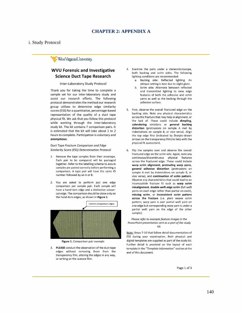
140
CHAPTER 2: APPENDIX A
i. Study Protocol
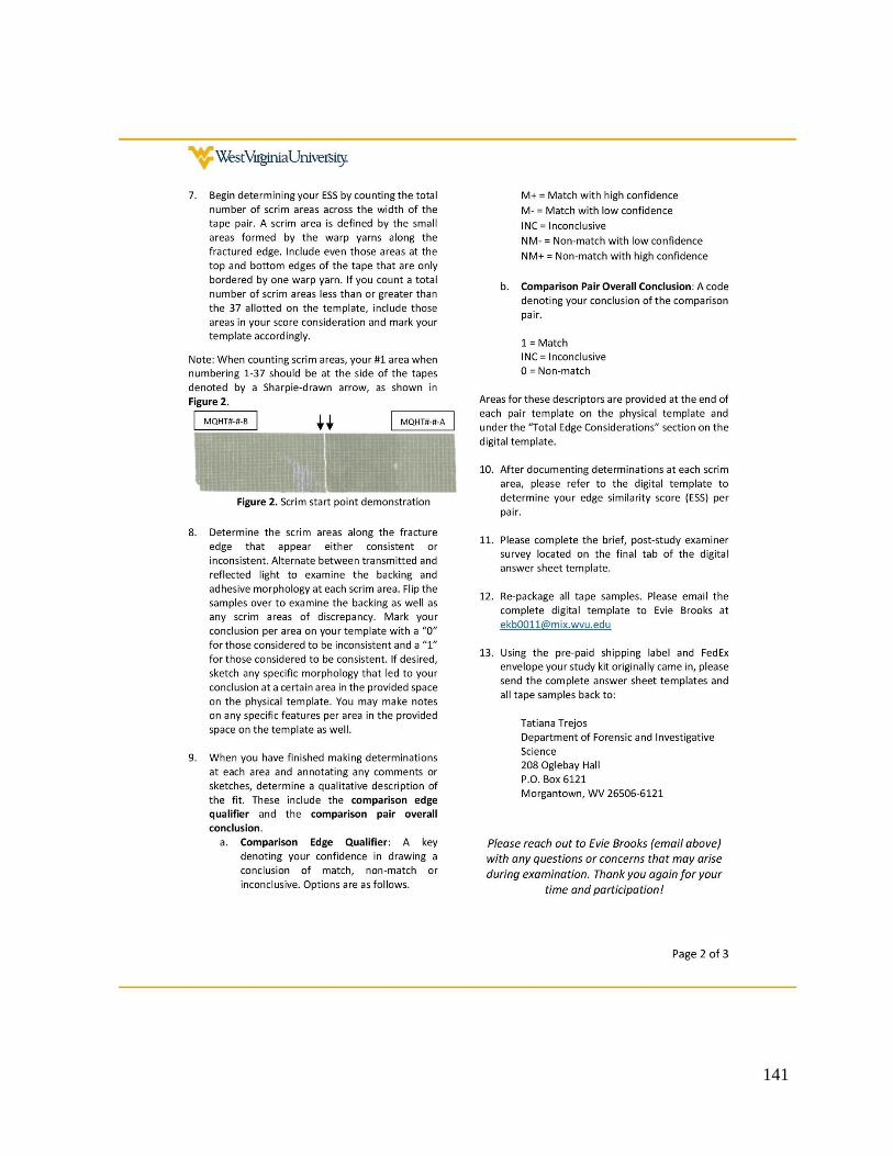
141
142

143
ii. Physical scrim documentation template

144

145

146

147
iii. Digital scrim documentation template (1 of 8 worksheets, one per pair and a final survey tab)

148
iv. Instructional PowerPoint presentation
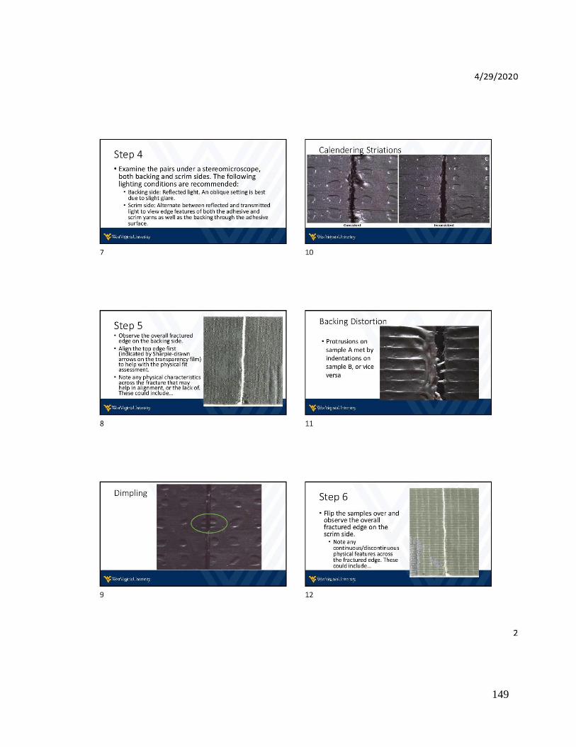
149
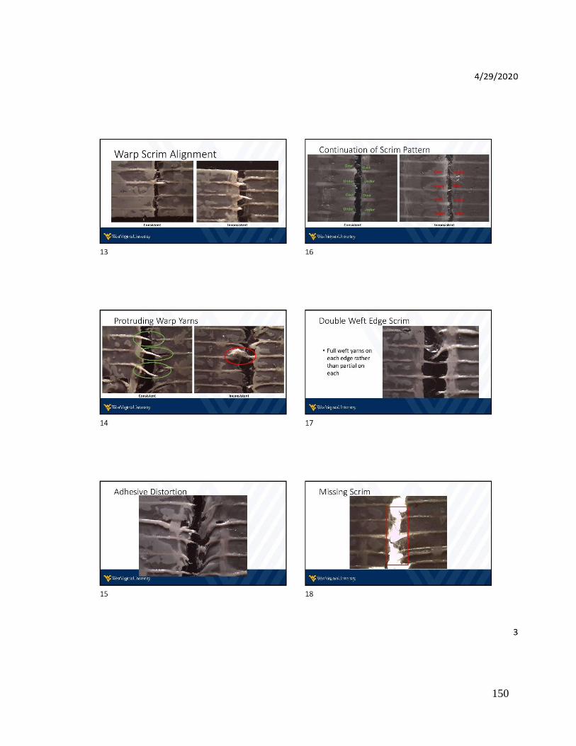
150

151

152
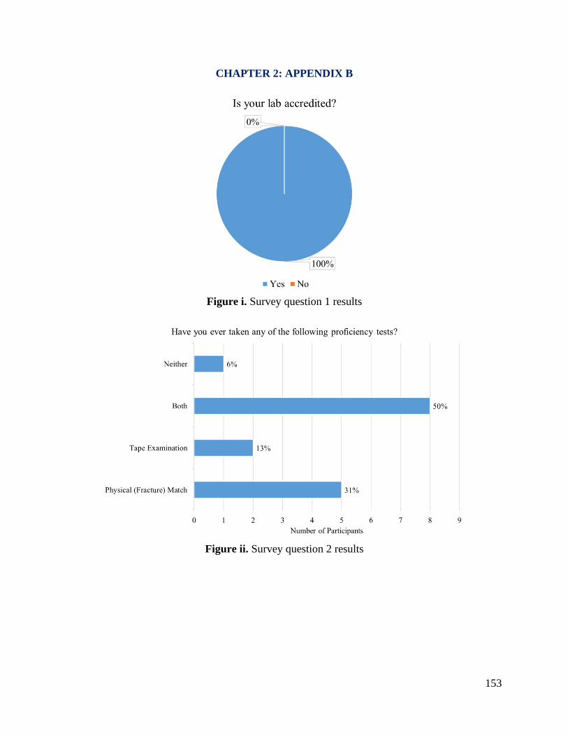
153
CHAPTER 2: APPENDIX B
Figure i. Survey question 1 results
Figure ii. Survey question 2 results
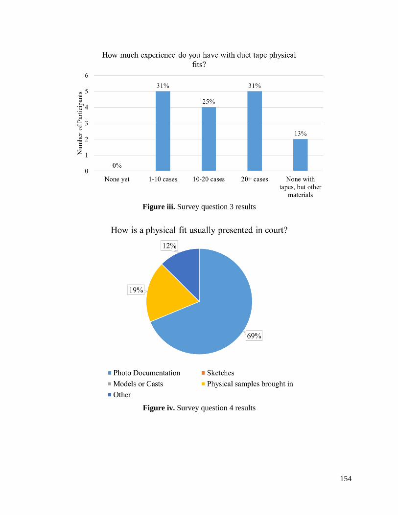
154
Figure iii. Survey question 3 results
Figure iv. Survey question 4 results
155
Figure v. Survey question 5 results
Figure vi. Survey question 6 results
156
Figure vii. Survey question 7 results
Figure viii. Survey question 8 results
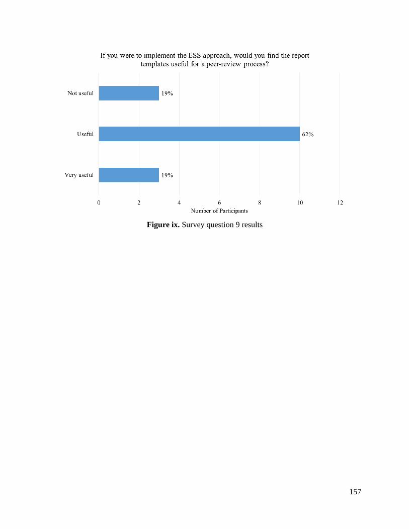
157
Figure ix. Survey question 9 results
158
IV. CHAPTER THREE
Steps Toward Quantitative Assessment of Textile Physical Fits – Expansion of
the Edge Similarity Score (ESS) Method
1. Overview of Textile Fracture Study
Following the development of a systematic, quantitative, score-based edge similarity score (ESS)
method of assessment for physical fits in duct tape samples by our research group, this project
aims to extend assessment of the method’s suitability into other trace material types. Textiles were
selected as the initial material expansion due to their prevalence in clothing and household textile
items, and their potential to be fractured during the commission of a crime. While the initial
experimental design involved the assessment of 100 comparison pairs of hand-torn, 100% jersey-
knit polyester, a high level of disagreement in overall physical fit conclusion was observed
between two examiners in just the first 37 pairs of the sample set (74 comparisons, 37 per
examiner). Likewise, unacceptable high false negatives (29 out of 46, 63% false negative rate)
were observed that required the evaluation of the causes of such error rates. Through this first
dataset, it was evident that the assessment of suitability prior to examination of physical fits was
imperative in textile samples. In the absence of consensus guides to assess suitability in current
practice, the goal of our study was redirected to begin to answer more fundamental questions.
Therefore, it was determined a baseline study assessing accuracy of the ESS method when applied
to textile items of various compositions, constructions, and separation methods was needed in
order to determine those textiles exhibiting sufficient distinctive edge characteristics for physical
fit alignment.
A sample set of 100 comparison pairs was then created consisting of five textile items: 1) Item A,
a pair of men’s navy dress pants composed of 75% polyester and 25% cotton in a twill weave
construction; 2) Item B, a pair of women’s blue jeans composed of 60% cotton, 22% rayon, 17%
polyester, and 1% spandex in a twill weave construction; 3) Item C, a men’s blue-striped, short
sleeve button-up shirt composed of 100% cotton in a plain weave construction; 4) Item D, a beige
women’s tank top composed of 100% polyester in a satin weave construction; and 5) Item E, a
blue and white patterned, short sleeve women’s top composed of 93% rayon and 7% flax in a
jersey knit construction. Twenty comparison pairs were prepared from each textile item, with ten
each being separated through hand-tearing and stabbing, respectively. All sample pairs were re-
labelled and re-organized by external researchers who were not participating in pair assessment to
reduce potential bias. Then, two examiners blind to the ground truth of the sample set participated
in examination of the fracture edges and estimation of the ESS. The ESS method was adapted for
textile examination as each edge was divided into 10 equal bins or units by overall fracture edge
length. In addition to “1” (match) and “0” (non-match) decisions per unit, three weighting factors
were potentially attributed to each bin due to the presence of distinctive characteristics described
in further detail below. This led to the determination of an initial ESS, weighted ESS, and rarity
ratio for each comparison pair. In addition, frequency of occurrence of all noted distinctive
characteristics were documented as a preliminary effort to evaluate the rarity of observed features
159
across the fracture edges.
Throughout the examination process, examiner notes indicated the following general
characteristics that became useful in their edge assessments: color, fabric construction, general
fiber size and shape, fiber twist, alignment of long and short threads, and general fluorescence.
The following distinctive characteristics were noted as features attributing to the addition of
weighting factors: pattern continuation across fracture, stains, fabric damage, protrusions or gaps,
and partial pattern fluorescence.
Overall, 93% accuracy was observed for the hand-torn set while 95% accuracy was observed for
the stabbed set. The hand-torn set resulted in an 8% false negative rate, 2% false positive rate, and
4% inconclusive (true match samples) rate. The stabbed set resulted in an 4% false negative rate,
0% false positive rate, 4% inconclusive (true match samples), and 2% inconclusive (true non-
match samples) rate. A higher misclassification rate was observed in the hand-torn set due to the
higher degree of distortion presented by the fraying and stretching contributed by the tearing
process. In addition, most misclassifications occurred within samples associated to Items D and E,
the women’s tan tank top composed of 100% polyester and the navy patterned women’s jersey-
knit top. Both items attributed higher levels of stretch than the other garments. These results
indicate that textile items with fabric types of higher elasticity, due to either fabric construction or
fiber composition, may present limited fracture fit analysis capabilities and examiners should be
aware of potential sources of uncertainty on their conclusions.
2. Introduction
Due to the prevalence of clothing items and household textiles in everyday use, textile items are
materials commonly present at the scene of a crime. Depending upon the interaction of the textile
item with individuals present during the commission of a crime, textile analysis can become a
critical link between individuals, objects, and locations. In situations involving assault or
homicide, both victim and suspect garments can become damaged and separated through tearing
or shearing. Garments can also become damaged or fractured as the result of a hit-and-run, fire
exposure, or long period of submersion in water. When violence occurs in the home, common
household textiles such as bedsheets, curtains, or towels can become fractured as well. These
situations lead to forensic textile examinations for the determination of textile damage source (i.e.
stabbing, cutting, or tearing) as well as alignment of textile remains in the analysis of a potential
fracture fit. Foreign fibers discovered at the scene or on collected textile materials can also be
compared to known fibers collected from suspect garments to attribute a common source or to
differentiate.1
Within the physical fit literature, case reports highlight the variety of situations in which a textile
physical fit provided a useful link in an investigation. For example, Fisher et al. described multiple
textile physical fit analyses: a case in which T-shirt fragments from the victim’s hands were later
compared to the suspect’s recovered torn shirt; a situation in which a hit-and-run victim’s torn coat
was compared to a piece of fabric collected from the front fender of the suspect’s car; and an
160
additional scenario that involved a torn fabric fragment discovered at the point of entry of a
burglary scene that was later compared to the suspect’s torn clothing2. In addition to these, Shor et
al. shared a case in which a physical fit examination was responsible for the confirmation of stolen
artwork. Examiners were able to physically fit questioned cut canvas edges to the known fragments
remaining in the original frames due to the edge morphology features presented by the manipulated
canvas3.
When damaged textiles are received in a forensic laboratory, examination typically begins with
visual examinations of the fracture at both the macro and microscopic levels to determine if a
potential physical fit exists. Often, if the edges align and the textiles appear consistent in physical
features such as color, construction, and weave/knit pattern, this will be considered the highest
level of association and further analysis will not often occur4. Some laboratories will still carry out
a full analytical scheme, documenting the physical properties of both the questioned and known
textile samples as well as the optical properties and chemical composition properties through
instrumental determination of polymer and dye type.
In addition to physical and chemical analysis, some laboratories will perform damage source
determinations on the fractured textiles. This usually involves viewing fractured edge cross-
sectional morphology of textile fibers through either stereomicroscopy or scanning electron
microscopy (SEM). Fiber cross-sectional shape after a fracture event has been shown to exhibit
specific shapes, such as a “pinched” appearance following a shearing or a “mushroom cap”
appearance following a tear. Source of damage analysis may also be accompanied by laboratory-
based simulations or recreations of the suspected fracture event to compare fractured fiber
morphology.5
Textile damage source determination is a well-researched niche within the trace evidence
discipline. For example, Kemp et al.6 provided a damage determination study in apparel fabrics.
The authors subjected two fabric types (cotton bull drill, more commonly known as denim, and
cotton single jersey) at three levels of varying wear to stabbing events using three different
weapons – a kitchen knife, hunting knife, and screwdriver. Stabbing events were delivered through
two avenues: a human participant trial and an impact rig with each respective weapon. Fractured
fabric ends were then examined through stereomicroscopy, digital photography, and Scanning
Electron Microscopy (SEM) to determine if fabric morphology showed specific characteristics
revealing weapon type. It was found that weapon type could be determined from differences in
severance size and shape, degree of fabric distortion, position of severed yarn ends, loop snippets,
curled yarns, and the morphology of the fractured fibers. Directionality of the stab could only be
found if the upper and lower blade edges of the respective weapon had varying geometries, edge
types, or degrees of sharpness and no tearing occurred during the fracture6. A similar SEM source-
determination study was presented for fibers by Pelton7. In this study, nylon fabric samples were
cut in the weft direction with scissors, a carving knife, and an Elmendorf tear machine. Fibers were
sampled from three different sites along the resulting fracture edge and analyzed through SEM for
source determination. Of the 600 analyzed fiber ends, 322 were categorized based on their shearing
method7.
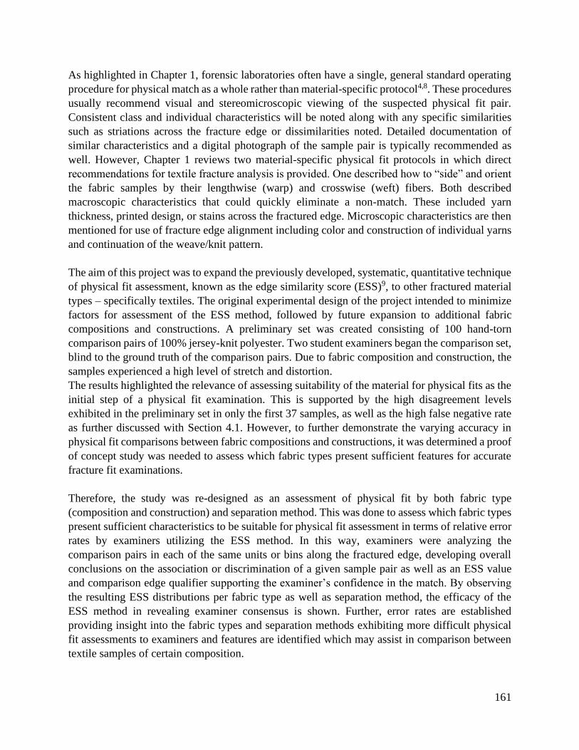
161
As highlighted in Chapter 1, forensic laboratories often have a single, general standard operating
procedure for physical match as a whole rather than material-specific protocol4,8. These procedures
usually recommend visual and stereomicroscopic viewing of the suspected physical fit pair.
Consistent class and individual characteristics will be noted along with any specific similarities
such as striations across the fracture edge or dissimilarities noted. Detailed documentation of
similar characteristics and a digital photograph of the sample pair is typically recommended as
well. However, Chapter 1 reviews two material-specific physical fit protocols in which direct
recommendations for textile fracture analysis is provided. One described how to “side” and orient
the fabric samples by their lengthwise (warp) and crosswise (weft) fibers. Both described
macroscopic characteristics that could quickly eliminate a non-match. These included yarn
thickness, printed design, or stains across the fractured edge. Microscopic characteristics are then
mentioned for use of fracture edge alignment including color and construction of individual yarns
and continuation of the weave/knit pattern.
The aim of this project was to expand the previously developed, systematic, quantitative technique
of physical fit assessment, known as the edge similarity score (ESS)9, to other fractured material
types – specifically textiles. The original experimental design of the project intended to minimize
factors for assessment of the ESS method, followed by future expansion to additional fabric
compositions and constructions. A preliminary set was created consisting of 100 hand-torn
comparison pairs of 100% jersey-knit polyester. Two student examiners began the comparison set,
blind to the ground truth of the comparison pairs. Due to fabric composition and construction, the
samples experienced a high level of stretch and distortion.
The results highlighted the relevance of assessing suitability of the material for physical fits as the
initial step of a physical fit examination. This is supported by the high disagreement levels
exhibited in the preliminary set in only the first 37 samples, as well as the high false negative rate
as further discussed with Section 4.1. However, to further demonstrate the varying accuracy in
physical fit comparisons between fabric compositions and constructions, it was determined a proof
of concept study was needed to assess which fabric types present sufficient features for accurate
fracture fit examinations.
Therefore, the study was re-designed as an assessment of physical fit by both fabric type
(composition and construction) and separation method. This was done to assess which fabric types
present sufficient characteristics to be suitable for physical fit assessment in terms of relative error
rates by examiners utilizing the ESS method. In this way, examiners were analyzing the
comparison pairs in each of the same units or bins along the fractured edge, developing overall
conclusions on the association or discrimination of a given sample pair as well as an ESS value
and comparison edge qualifier supporting the examiner’s confidence in the match. By observing
the resulting ESS distributions per fabric type as well as separation method, the efficacy of the
ESS method in revealing examiner consensus is shown. Further, error rates are established
providing insight into the fabric types and separation methods exhibiting more difficult physical
fit assessments to examiners and features are identified which may assist in comparison between
textile samples of certain composition.
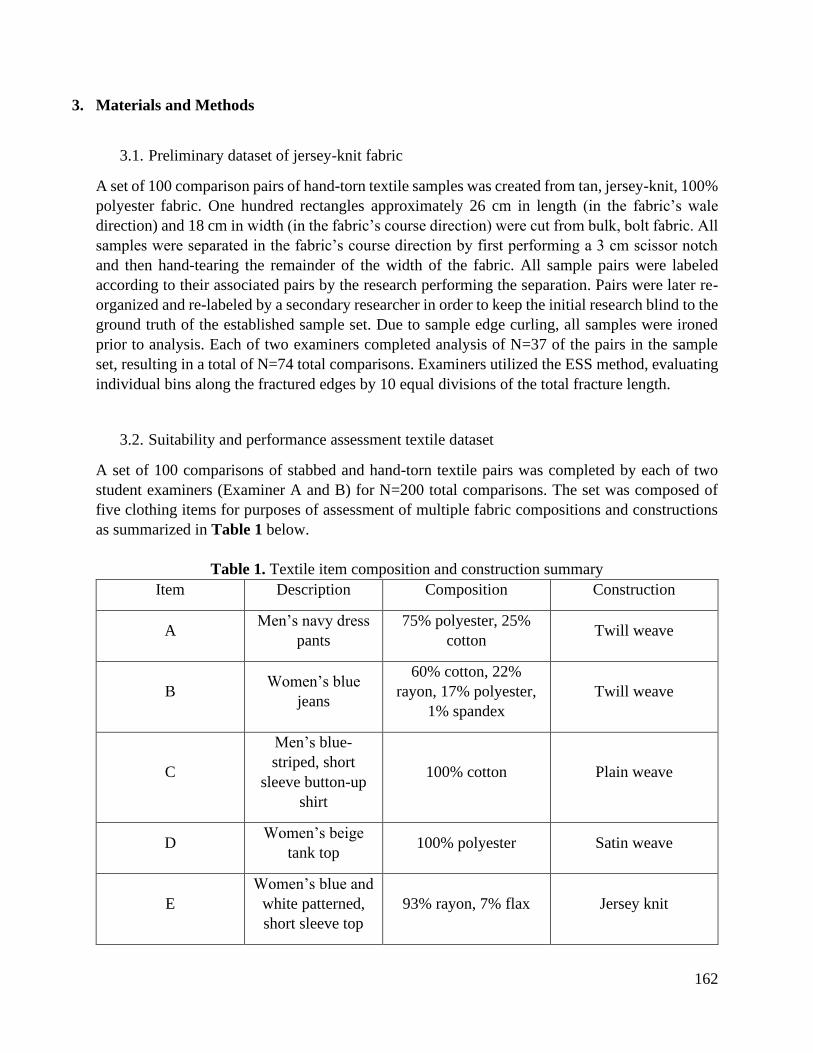
162
3. Materials and Methods
3.1. Preliminary dataset of jersey-knit fabric
A set of 100 comparison pairs of hand-torn textile samples was created from tan, jersey-knit, 100%
polyester fabric. One hundred rectangles approximately 26 cm in length (in the fabric’s wale
direction) and 18 cm in width (in the fabric’s course direction) were cut from bulk, bolt fabric. All
samples were separated in the fabric’s course direction by first performing a 3 cm scissor notch
and then hand-tearing the remainder of the width of the fabric. All sample pairs were labeled
according to their associated pairs by the research performing the separation. Pairs were later re-
organized and re-labeled by a secondary researcher in order to keep the initial research blind to the
ground truth of the established sample set. Due to sample edge curling, all samples were ironed
prior to analysis. Each of two examiners completed analysis of N=37 of the pairs in the sample
set, resulting in a total of N=74 total comparisons. Examiners utilized the ESS method, evaluating
individual bins along the fractured edges by 10 equal divisions of the total fracture length.
3.2. Suitability and performance assessment textile dataset
A set of 100 comparisons of stabbed and hand-torn textile pairs was completed by each of two
student examiners (Examiner A and B) for N=200 total comparisons. The set was composed of
five clothing items for purposes of assessment of multiple fabric compositions and constructions
as summarized in Table 1 below.
Table 1. Textile item composition and construction summary
Item Description Composition Construction
A Men’s navy dress
pants
75% polyester, 25%
cotton Twill weave
B Women’s blue
jeans
60% cotton, 22%
rayon, 17% polyester,
1% spandex
Twill weave
C
Men’s blue-
striped, short
sleeve button-up
shirt
100% cotton Plain weave
D Women’s beige
tank top 100% polyester Satin weave
E
Women’s blue and
white patterned,
short sleeve top
93% rayon, 7% flax Jersey knit
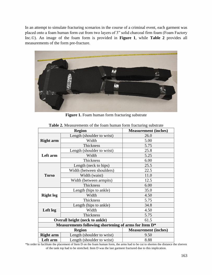
163
In an attempt to simulate fracturing scenarios in the course of a criminal event, each garment was
placed onto a foam human form cut from two layers of 3” solid charcoal firm foam (Foam Factory
Inc.©). An image of the foam form is provided in Figure 1, while Table 2 provides all
measurements of the form pre-fracture.
Figure 1. Foam human form fracturing substrate
Table 2. Measurements of the foam human form fracturing substrate
Region Measurement (inches)
Right arm
Length (shoulder to wrist) 26.0
Width 5.00
Thickness 5.75
Left arm
Length (shoulder to wrist) 25.8
Width 5.25
Thickness 6.00
Torso
Length (neck to hips) 25.5
Width (between shoulders) 22.5
Width (waist) 11.0
Width (between armpits) 12.5
Thickness 6.00
Right leg
Length (hips to ankle) 35.0
Width 4.50
Thickness 5.75
Left leg
Length (hips to ankle) 34.8
Width 4.50
Thickness 5.75
Overall height (neck to ankle) 61.5
Measurements following shortening of arms for Item D*
Region Measurement (inches)
Right arm Length (shoulder to wrist) 9.50
Left arm Length (shoulder to wrist) 8.88 *In order to facilitate the placement of Item D on the foam human form, the arms had to be cut to shorten the distance the sleeves
of the tank top had to be stretched. Item D was the last garment fractured due to this implication.
164
The front of each garment was stabbed ten times with a Cuisinart® Classic 8” chef’s knife at five
each of horizontal and vertical orientations. A plastic guard was adhered to the blade at 2.5” from
the tip to maintain consistent stab depth. Between stabbings, the plastic guard was repositioned to
its original distance if any movement had occurred. Measurements were taken of the plastic guard
position both pre- and post-stabbing to assess movement. Mean distance travelled by the guard
during all stabbing events was 1.39 ± 0.38 inches.
A single researcher performed each stabbing with their right arm oriented at a 90° angle, with
distance from knife tip to “chest” surface measured with each replicate to maintain consistency.
Distance of knife tip to garment surface was measured prior to each stabbing event. Mean distance
through the stabbing process was 19.25 ± 1.56”. Each item was then hand-torn ten times on
different locations, at five each of horizontal and vertical orientations by a secondary researcher.
A pair of scissors was used to create a 0.75” notch in the tear location and the researcher proceeded
by pulling each edge of the notch apart to create the hand tear.
All fractures were cut from the garments, reorganized, and labelled by student volunteers so
examiners would remain blind to the ground truth of the fractured sample pairs. An inventory of
the original identification numbers was then created to maintain the traceability of the samples,
and a random number generator was used to relabel the items with a unique identifier and to mix
the fracture edges to generate a relatively balanced number of true mated and true non-mated
samples. Two examiners then completed the physical examination of the sample set of 100
comparison pairs, 20 pairs per garment with 10 each of stabbed and hand-torn fractures. A
schematic of the experimental design can be observed in Figure 2 below.
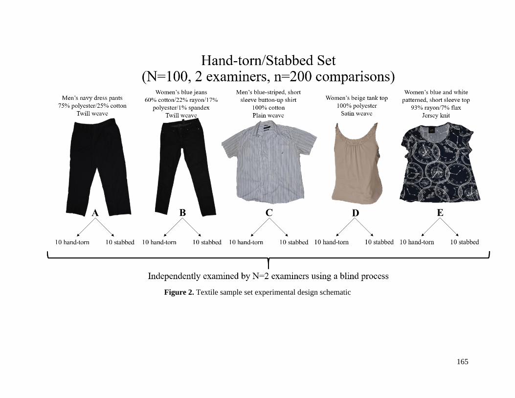
165
Figure 2. Textile sample set experimental design schematic
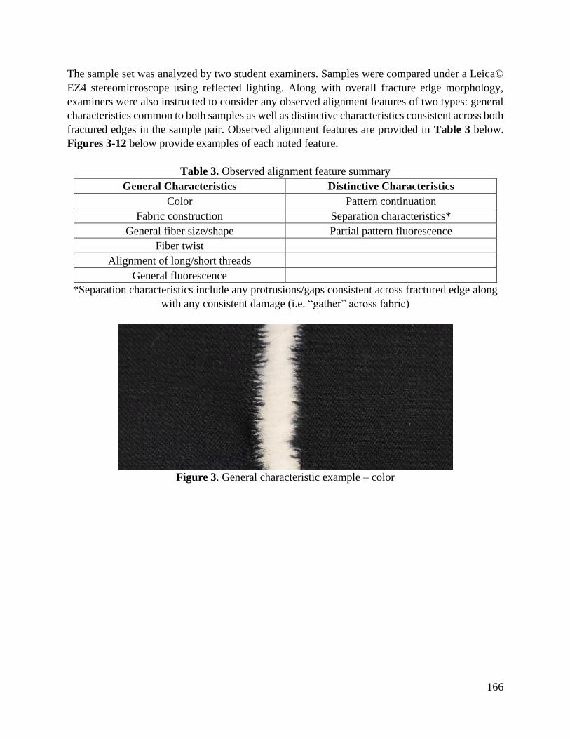
166
The sample set was analyzed by two student examiners. Samples were compared under a Leica©
EZ4 stereomicroscope using reflected lighting. Along with overall fracture edge morphology,
examiners were also instructed to consider any observed alignment features of two types: general
characteristics common to both samples as well as distinctive characteristics consistent across both
fractured edges in the sample pair. Observed alignment features are provided in Table 3 below.
Figures 3-12 below provide examples of each noted feature.
Table 3. Observed alignment feature summary
General Characteristics Distinctive Characteristics
Color Pattern continuation
Fabric construction Separation characteristics*
General fiber size/shape Partial pattern fluorescence
Fiber twist
Alignment of long/short threads
General fluorescence
*Separation characteristics include any protrusions/gaps consistent across fractured edge along
with any consistent damage (i.e. “gather” across fabric)
Figure 3. General characteristic example – color
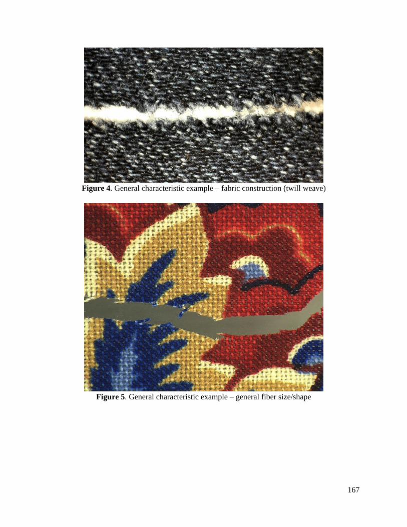
167
Figure 4. General characteristic example – fabric construction (twill weave)
Figure 5. General characteristic example – general fiber size/shape
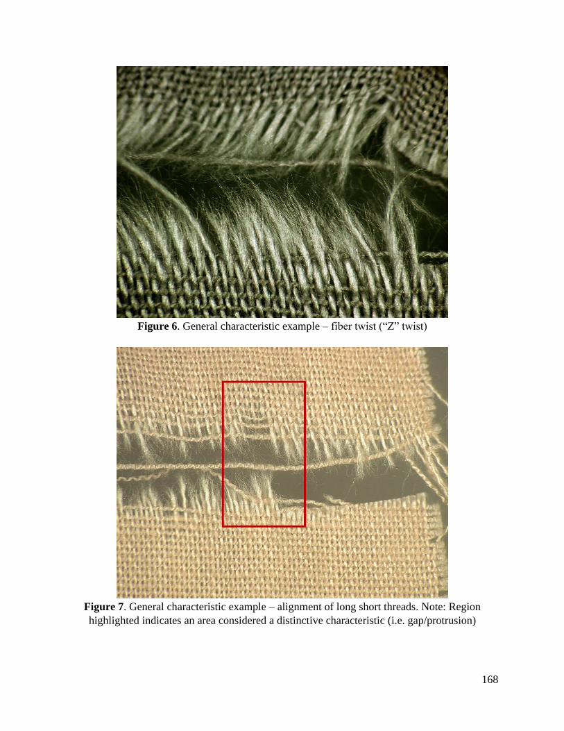
168
Figure 6. General characteristic example – fiber twist (“Z” twist)
Figure 7. General characteristic example – alignment of long short threads. Note: Region
highlighted indicates an area considered a distinctive characteristic (i.e. gap/protrusion)
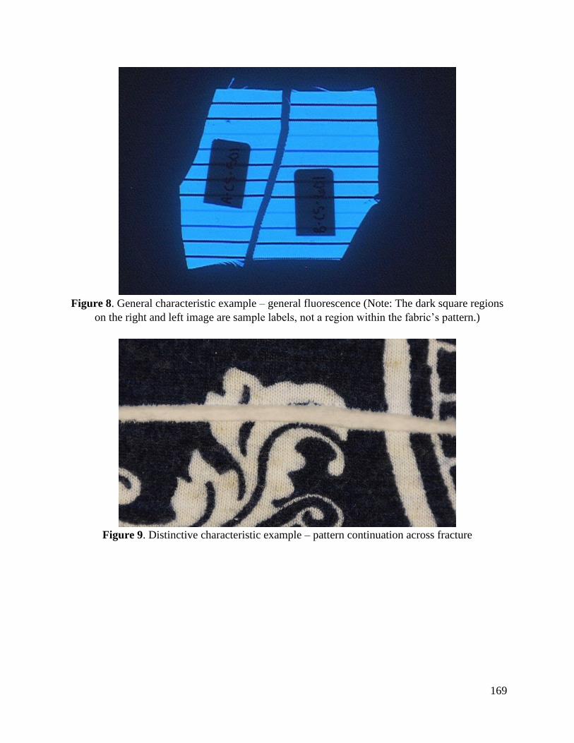
169
Figure 8. General characteristic example – general fluorescence (Note: The dark square regions
on the right and left image are sample labels, not a region within the fabric’s pattern.)
Figure 9. Distinctive characteristic example – pattern continuation across fracture
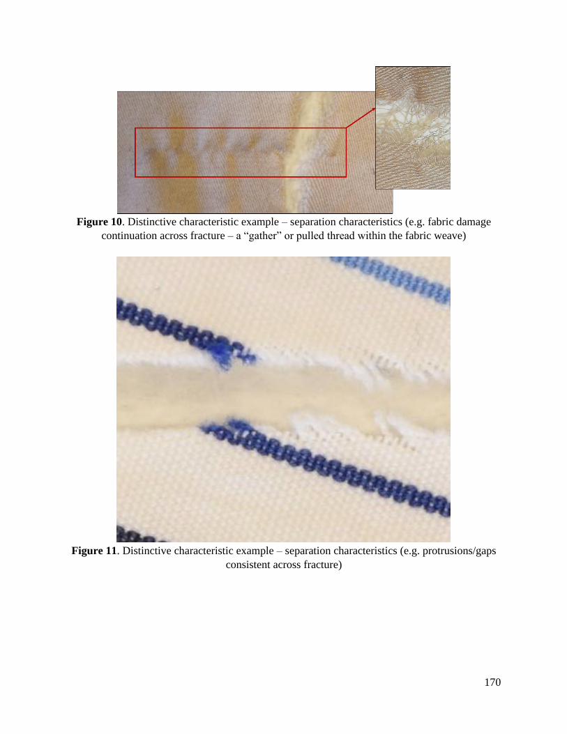
170
Figure 10. Distinctive characteristic example – separation characteristics (e.g. fabric damage
continuation across fracture – a “gather” or pulled thread within the fabric weave)
Figure 11. Distinctive characteristic example – separation characteristics (e.g. protrusions/gaps
consistent across fracture)
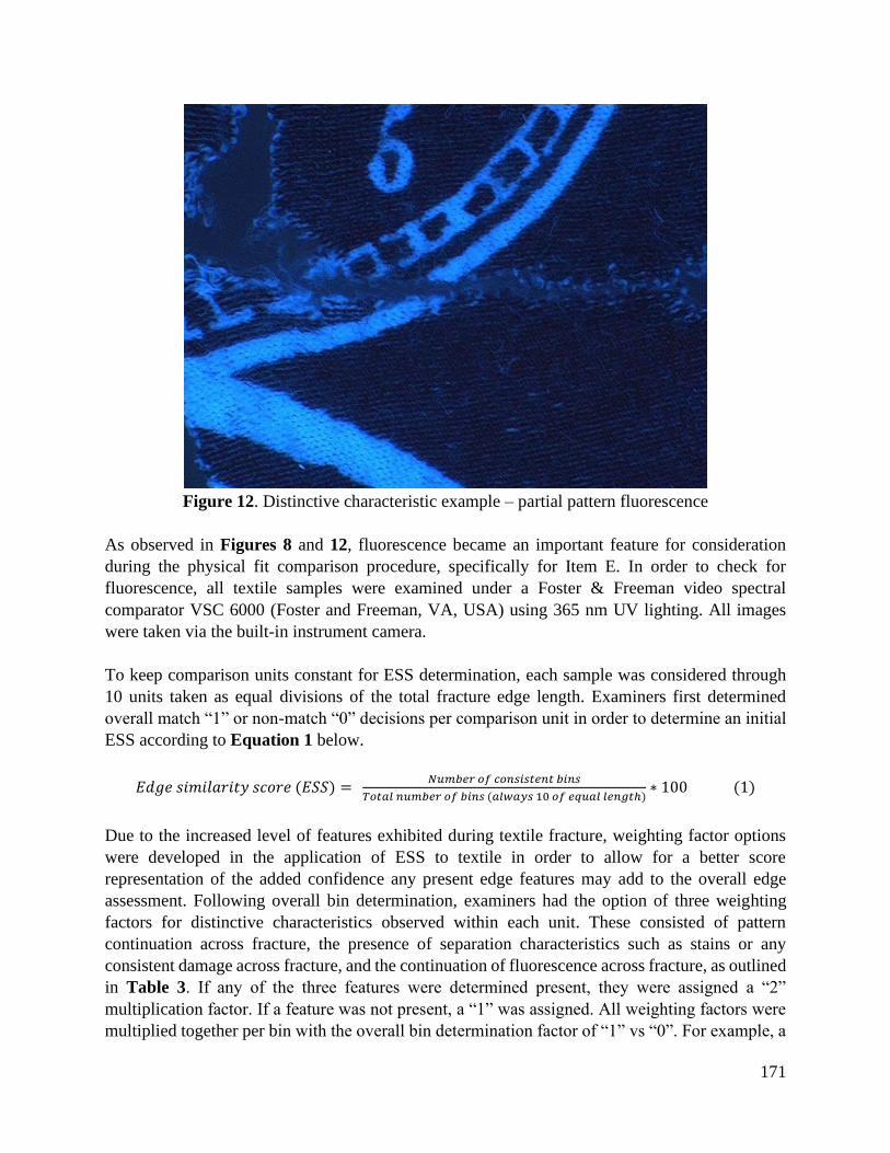
171
Figure 12. Distinctive characteristic example – partial pattern fluorescence
As observed in Figures 8 and 12, fluorescence became an important feature for consideration
during the physical fit comparison procedure, specifically for Item E. In order to check for
fluorescence, all textile samples were examined under a Foster & Freeman video spectral
comparator VSC 6000 (Foster and Freeman, VA, USA) using 365 nm UV lighting. All images
were taken via the built-in instrument camera.
To keep comparison units constant for ESS determination, each sample was considered through
10 units taken as equal divisions of the total fracture edge length. Examiners first determined
overall match “1” or non-match “0” decisions per comparison unit in order to determine an initial
ESS according to Equation 1 below.
𝐸𝑑𝑔𝑒 𝑠𝑖𝑚𝑖𝑙𝑎𝑟𝑖𝑡𝑦 𝑠𝑐𝑜𝑟𝑒 (𝐸𝑆𝑆) = 𝑁𝑢𝑚𝑏𝑒𝑟 𝑜𝑓 𝑐𝑜𝑛𝑠𝑖𝑠𝑡𝑒𝑛𝑡 𝑏𝑖𝑛𝑠
𝑇𝑜𝑡𝑎𝑙 𝑛𝑢𝑚𝑏𝑒𝑟 𝑜𝑓 𝑏𝑖𝑛𝑠 (𝑎𝑙𝑤𝑎𝑦𝑠 10 𝑜𝑓 𝑒𝑞𝑢𝑎𝑙 𝑙𝑒𝑛𝑔𝑡ℎ)∗ 100 (1)
Due to the increased level of features exhibited during textile fracture, weighting factor options
were developed in the application of ESS to textile in order to allow for a better score
representation of the added confidence any present edge features may add to the overall edge
assessment. Following overall bin determination, examiners had the option of three weighting
factors for distinctive characteristics observed within each unit. These consisted of pattern
continuation across fracture, the presence of separation characteristics such as stains or any
consistent damage across fracture, and the continuation of fluorescence across fracture, as outlined
in Table 3. If any of the three features were determined present, they were assigned a “2”
multiplication factor. If a feature was not present, a “1” was assigned. All weighting factors were
multiplied together per bin with the overall bin determination factor of “1” vs “0”. For example, a
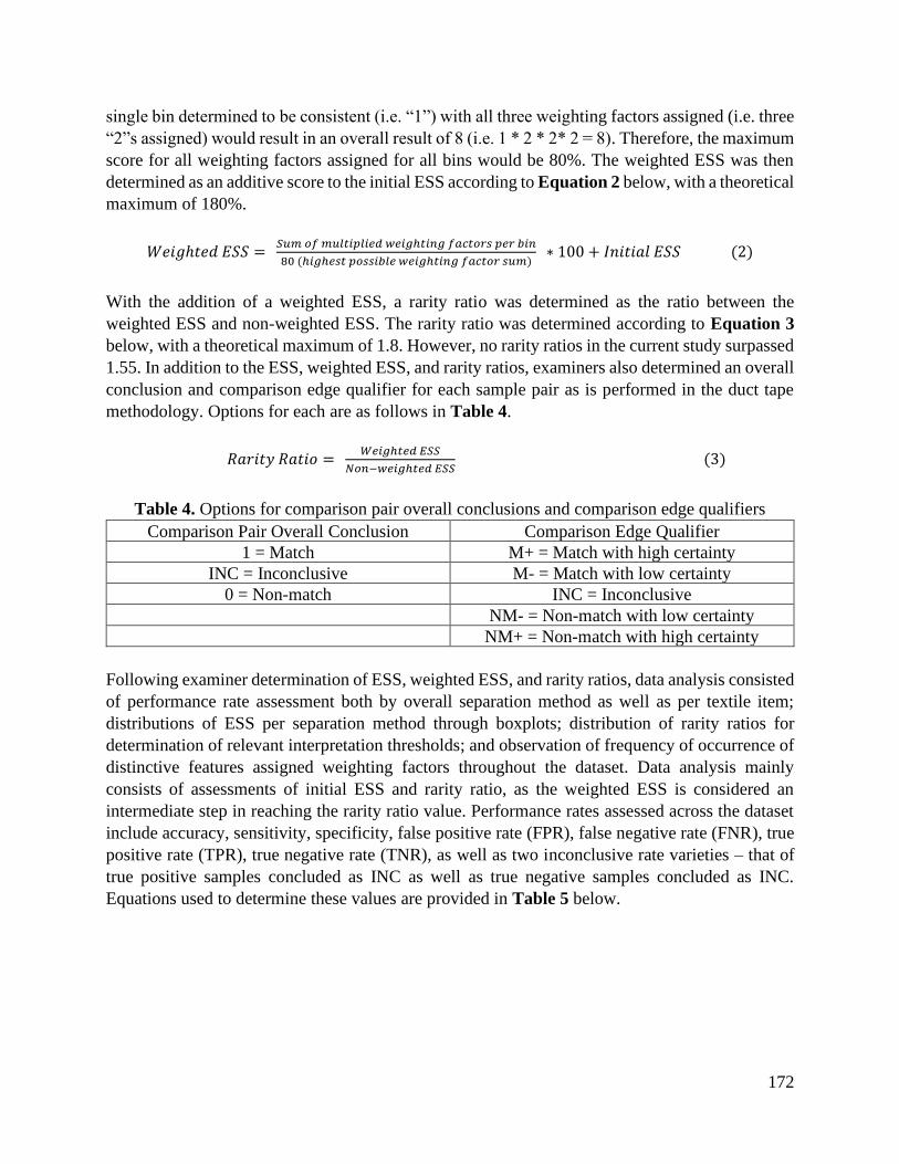
172
single bin determined to be consistent (i.e. “1”) with all three weighting factors assigned (i.e. three
“2”s assigned) would result in an overall result of 8 (i.e. 1 * 2 * 2* 2 = 8). Therefore, the maximum
score for all weighting factors assigned for all bins would be 80%. The weighted ESS was then
determined as an additive score to the initial ESS according to Equation 2 below, with a theoretical
maximum of 180%.
𝑊𝑒𝑖𝑔ℎ𝑡𝑒𝑑 𝐸𝑆𝑆 = 𝑆𝑢𝑚 𝑜𝑓 𝑚𝑢𝑙𝑡𝑖𝑝𝑙𝑖𝑒𝑑 𝑤𝑒𝑖𝑔ℎ𝑡𝑖𝑛𝑔 𝑓𝑎𝑐𝑡𝑜𝑟𝑠 𝑝𝑒𝑟 𝑏𝑖𝑛
80 (ℎ𝑖𝑔ℎ𝑒𝑠𝑡 𝑝𝑜𝑠𝑠𝑖𝑏𝑙𝑒 𝑤𝑒𝑖𝑔ℎ𝑡𝑖𝑛𝑔 𝑓𝑎𝑐𝑡𝑜𝑟 𝑠𝑢𝑚) ∗ 100 + 𝐼𝑛𝑖𝑡𝑖𝑎𝑙 𝐸𝑆𝑆 (2)
With the addition of a weighted ESS, a rarity ratio was determined as the ratio between the
weighted ESS and non-weighted ESS. The rarity ratio was determined according to Equation 3
below, with a theoretical maximum of 1.8. However, no rarity ratios in the current study surpassed
1.55. In addition to the ESS, weighted ESS, and rarity ratios, examiners also determined an overall
conclusion and comparison edge qualifier for each sample pair as is performed in the duct tape
methodology. Options for each are as follows in Table 4.
𝑅𝑎𝑟𝑖𝑡𝑦 𝑅𝑎𝑡𝑖𝑜 = 𝑊𝑒𝑖𝑔ℎ𝑡𝑒𝑑 𝐸𝑆𝑆
𝑁𝑜𝑛−𝑤𝑒𝑖𝑔ℎ𝑡𝑒𝑑 𝐸𝑆𝑆 (3)
Table 4. Options for comparison pair overall conclusions and comparison edge qualifiers
Comparison Pair Overall Conclusion Comparison Edge Qualifier
1 = Match M+ = Match with high certainty
INC = Inconclusive M- = Match with low certainty
0 = Non-match INC = Inconclusive
NM- = Non-match with low certainty
NM+ = Non-match with high certainty
Following examiner determination of ESS, weighted ESS, and rarity ratios, data analysis consisted
of performance rate assessment both by overall separation method as well as per textile item;
distributions of ESS per separation method through boxplots; distribution of rarity ratios for
determination of relevant interpretation thresholds; and observation of frequency of occurrence of
distinctive features assigned weighting factors throughout the dataset. Data analysis mainly
consists of assessments of initial ESS and rarity ratio, as the weighted ESS is considered an
intermediate step in reaching the rarity ratio value. Performance rates assessed across the dataset
include accuracy, sensitivity, specificity, false positive rate (FPR), false negative rate (FNR), true
positive rate (TPR), true negative rate (TNR), as well as two inconclusive rate varieties – that of
true positive samples concluded as INC as well as true negative samples concluded as INC.
Equations used to determine these values are provided in Table 5 below.
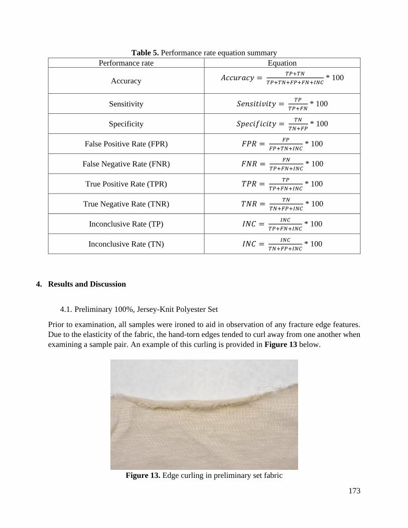
173
Table 5. Performance rate equation summary
Performance rate Equation
Accuracy
𝐴𝑐𝑐𝑢𝑟𝑎𝑐𝑦 = 𝑇𝑃+𝑇𝑁
𝑇𝑃+𝑇𝑁+𝐹𝑃+𝐹𝑁+𝐼𝑁𝐶 * 100
Sensitivity
𝑆𝑒𝑛𝑠𝑖𝑡𝑖𝑣𝑖𝑡𝑦 = 𝑇𝑃
𝑇𝑃+𝐹𝑁 * 100
Specificity
𝑆𝑝𝑒𝑐𝑖𝑓𝑖𝑐𝑖𝑡𝑦 = 𝑇𝑁
𝑇𝑁+𝐹𝑃 * 100
False Positive Rate (FPR)
𝐹𝑃𝑅 = 𝐹𝑃
𝐹𝑃+𝑇𝑁+𝐼𝑁𝐶 * 100
False Negative Rate (FNR)
𝐹𝑁𝑅 = 𝐹𝑁
𝑇𝑃+𝐹𝑁+𝐼𝑁𝐶 * 100
True Positive Rate (TPR)
𝑇𝑃𝑅 = 𝑇𝑃
𝑇𝑃+𝐹𝑁+𝐼𝑁𝐶 * 100
True Negative Rate (TNR)
𝑇𝑁𝑅 = 𝑇𝑁
𝑇𝑁+𝐹𝑃+𝐼𝑁𝐶 * 100
Inconclusive Rate (TP)
𝐼𝑁𝐶 = 𝐼𝑁𝐶
𝑇𝑃+𝐹𝑁+𝐼𝑁𝐶 * 100
Inconclusive Rate (TN)
𝐼𝑁𝐶 = 𝐼𝑁𝐶
𝑇𝑁+𝐹𝑃+𝐼𝑁𝐶 * 100
4. Results and Discussion
4.1. Preliminary 100%, Jersey-Knit Polyester Set
Prior to examination, all samples were ironed to aid in observation of any fracture edge features.
Due to the elasticity of the fabric, the hand-torn edges tended to curl away from one another when
examining a sample pair. An example of this curling is provided in Figure 13 below.
Figure 13. Edge curling in preliminary set fabric
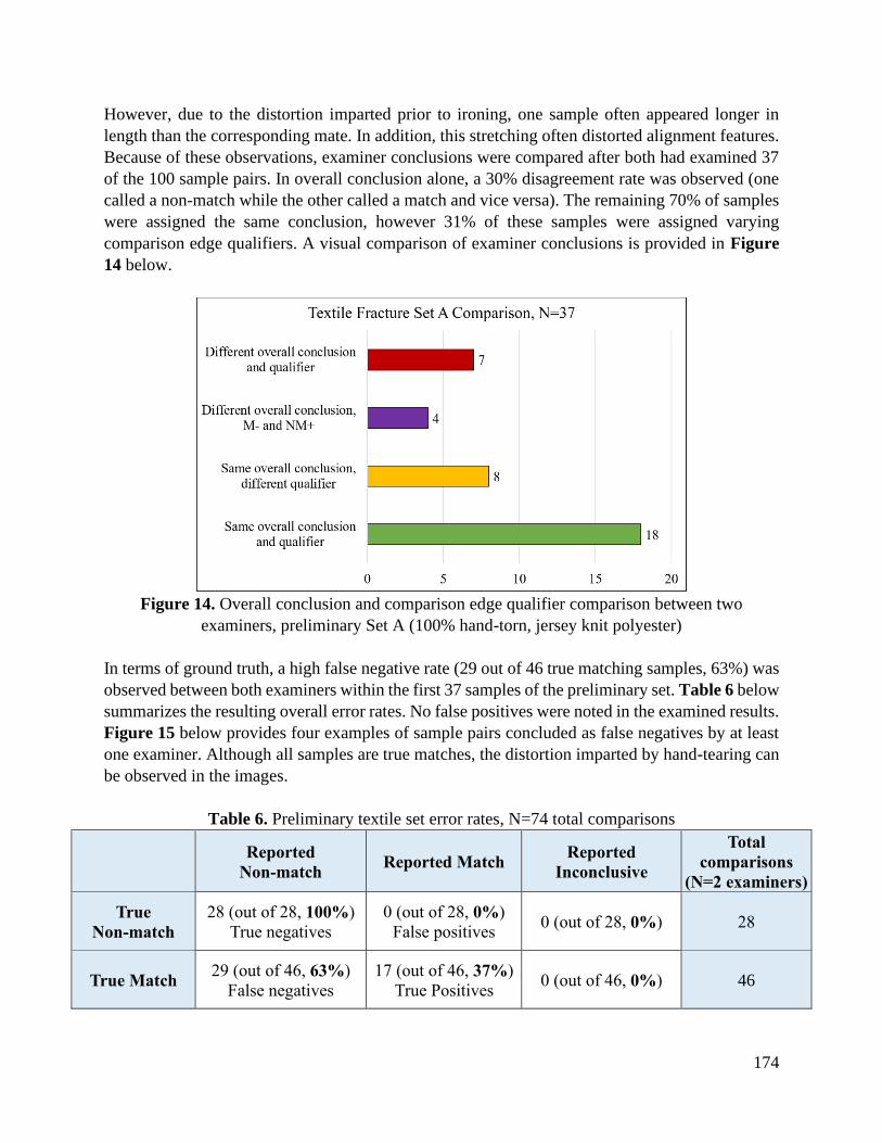
174
However, due to the distortion imparted prior to ironing, one sample often appeared longer in
length than the corresponding mate. In addition, this stretching often distorted alignment features.
Because of these observations, examiner conclusions were compared after both had examined 37
of the 100 sample pairs. In overall conclusion alone, a 30% disagreement rate was observed (one
called a non-match while the other called a match and vice versa). The remaining 70% of samples
were assigned the same conclusion, however 31% of these samples were assigned varying
comparison edge qualifiers. A visual comparison of examiner conclusions is provided in Figure
14 below.
Figure 14. Overall conclusion and comparison edge qualifier comparison between two
examiners, preliminary Set A (100% hand-torn, jersey knit polyester)
In terms of ground truth, a high false negative rate (29 out of 46 true matching samples, 63%) was
observed between both examiners within the first 37 samples of the preliminary set. Table 6 below
summarizes the resulting overall error rates. No false positives were noted in the examined results.
Figure 15 below provides four examples of sample pairs concluded as false negatives by at least
one examiner. Although all samples are true matches, the distortion imparted by hand-tearing can
be observed in the images.
Table 6. Preliminary textile set error rates, N=74 total comparisons
Reported
Non-match Reported Match
Reported
Inconclusive
Total
comparisons
(N=2 examiners)
True
Non-match
28 (out of 28, 100%)
True negatives
0 (out of 28, 0%)
False positives 0 (out of 28, 0%) 28
True Match 29 (out of 46, 63%)
False negatives
17 (out of 46, 37%)
True Positives 0 (out of 46, 0%) 46
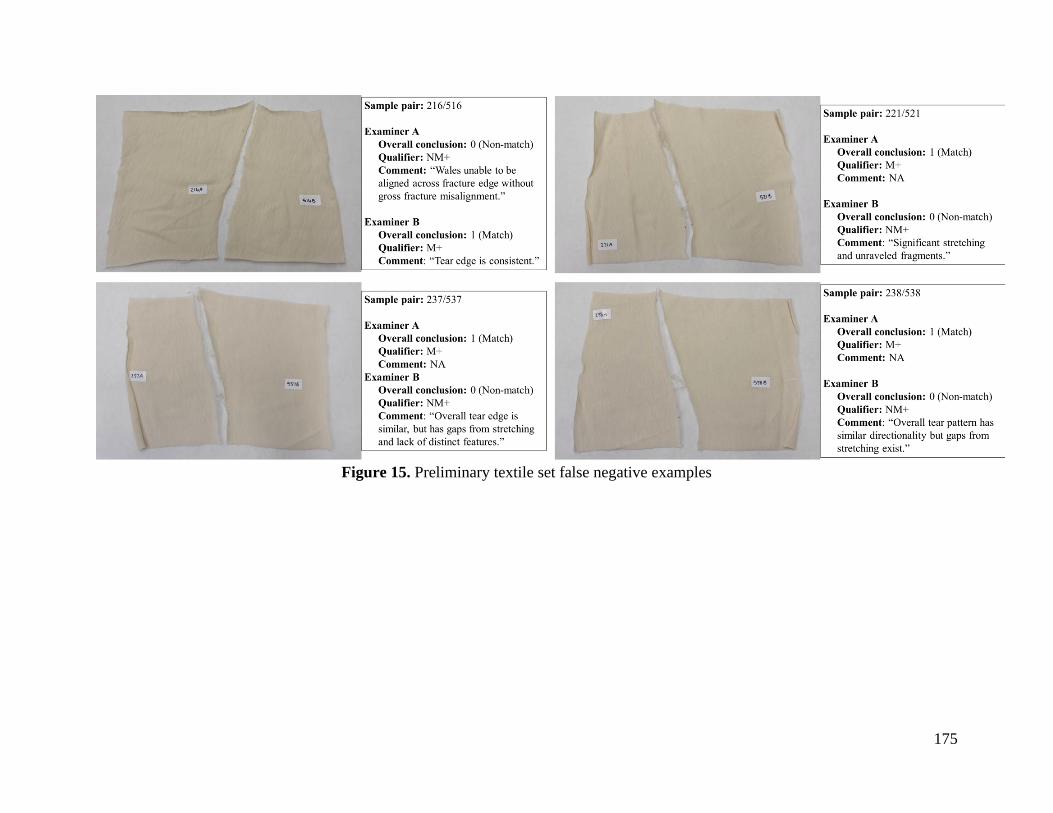
175
Figure 15. Preliminary textile set false negative examples
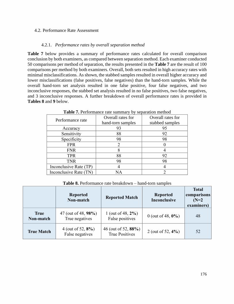
176
4.2. Performance Rate Assessment
4.2.1. Performance rates by overall separation method
Table 7 below provides a summary of performance rates calculated for overall comparison
conclusion by both examiners, as compared between separation method. Each examiner conducted
50 comparisons per method of separation, the results presented in the Table 7 are the result of 100
comparisons per method by both examiners. Overall, both sets resulted in high accuracy rates with
minimal misclassifications. As shown, the stabbed samples resulted in overall higher accuracy and
lower misclassifications (false positives, false negatives) than the hand-torn samples. While the
overall hand-torn set analysis resulted in one false positive, four false negatives, and two
inconclusive responses, the stabbed set analysis resulted in no false positives, two false negatives,
and 3 inconclusive responses. A further breakdown of overall performance rates is provided in
Tables 8 and 9 below.
Table 7. Performance rate summary by separation method
Performance rate Overall rates for
hand-torn samples
Overall rates for
stabbed samples
Accuracy 93 95
Sensitivity 88 92
Specificity 98 98
FPR 2 0
FNR 8 4
TPR 88 92
TNR 98 98
Inconclusive Rate (TP) 4 4
Inconclusive Rate (TN) NA 2
Table 8. Performance rate breakdown – hand-torn samples
Reported
Non-match Reported Match
Reported
Inconclusive
Total
comparisons
(N=2
examiners)
True
Non-match
47 (out of 48, 98%)
True negatives
1 (out of 48, 2%)
False positives 0 (out of 48, 0%) 48
True Match 4 (out of 52, 8%)
False negatives
46 (out of 52, 88%)
True Positives 2 (out of 52, 4%) 52
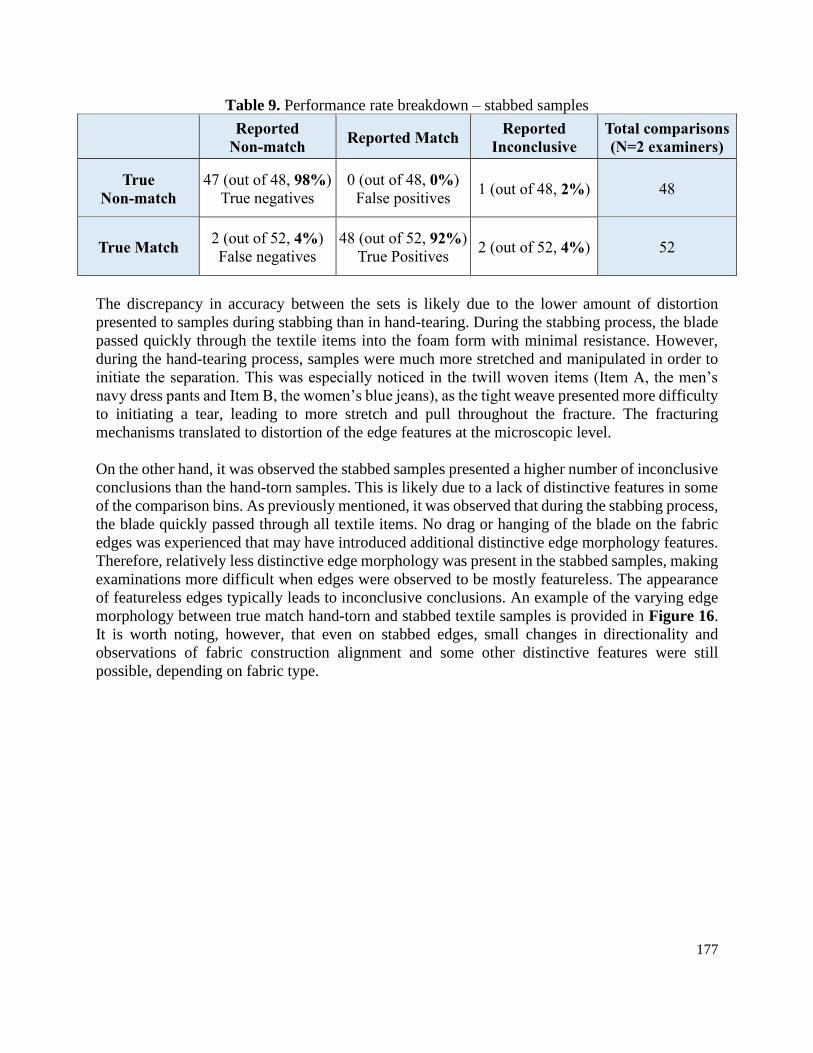
177
Table 9. Performance rate breakdown – stabbed samples
Reported
Non-match Reported Match
Reported
Inconclusive
Total comparisons
(N=2 examiners)
True
Non-match
47 (out of 48, 98%)
True negatives
0 (out of 48, 0%)
False positives 1 (out of 48, 2%) 48
True Match 2 (out of 52, 4%)
False negatives
48 (out of 52, 92%)
True Positives 2 (out of 52, 4%) 52
The discrepancy in accuracy between the sets is likely due to the lower amount of distortion
presented to samples during stabbing than in hand-tearing. During the stabbing process, the blade
passed quickly through the textile items into the foam form with minimal resistance. However,
during the hand-tearing process, samples were much more stretched and manipulated in order to
initiate the separation. This was especially noticed in the twill woven items (Item A, the men’s
navy dress pants and Item B, the women’s blue jeans), as the tight weave presented more difficulty
to initiating a tear, leading to more stretch and pull throughout the fracture. The fracturing
mechanisms translated to distortion of the edge features at the microscopic level.
On the other hand, it was observed the stabbed samples presented a higher number of inconclusive
conclusions than the hand-torn samples. This is likely due to a lack of distinctive features in some
of the comparison bins. As previously mentioned, it was observed that during the stabbing process,
the blade quickly passed through all textile items. No drag or hanging of the blade on the fabric
edges was experienced that may have introduced additional distinctive edge morphology features.
Therefore, relatively less distinctive edge morphology was present in the stabbed samples, making
examinations more difficult when edges were observed to be mostly featureless. The appearance
of featureless edges typically leads to inconclusive conclusions. An example of the varying edge
morphology between true match hand-torn and stabbed textile samples is provided in Figure 16.
It is worth noting, however, that even on stabbed edges, small changes in directionality and
observations of fabric construction alignment and some other distinctive features were still
possible, depending on fabric type.
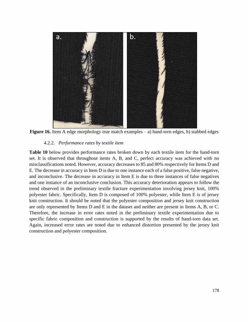
178
Figure 16. Item A edge morphology true match examples – a) hand-torn edges, b) stabbed edges
4.2.2. Performance rates by textile item
Table 10 below provides performance rates broken down by each textile item for the hand-torn
set. It is observed that throughout items A, B, and C, perfect accuracy was achieved with no
misclassifications noted. However, accuracy decreases to 85 and 80% respectively for Items D and
E. The decrease in accuracy in Item D is due to one instance each of a false positive, false negative,
and inconclusive. The decrease in accuracy in Item E is due to three instances of false negatives
and one instance of an inconclusive conclusion. This accuracy deterioration appears to follow the
trend observed in the preliminary textile fracture experimentation involving jersey knit, 100%
polyester fabric. Specifically, Item D is composed of 100% polyester, while Item E is of jersey
knit construction. It should be noted that the polyester composition and jersey knit construction
are only represented by Items D and E in the dataset and neither are present in Items A, B, or C.
Therefore, the increase in error rates noted in the preliminary textile experimentation due to
specific fabric composition and construction is supported by the results of hand-torn data set.
Again, increased error rates are noted due to enhanced distortion presented by the jersey knit
construction and polyester composition.
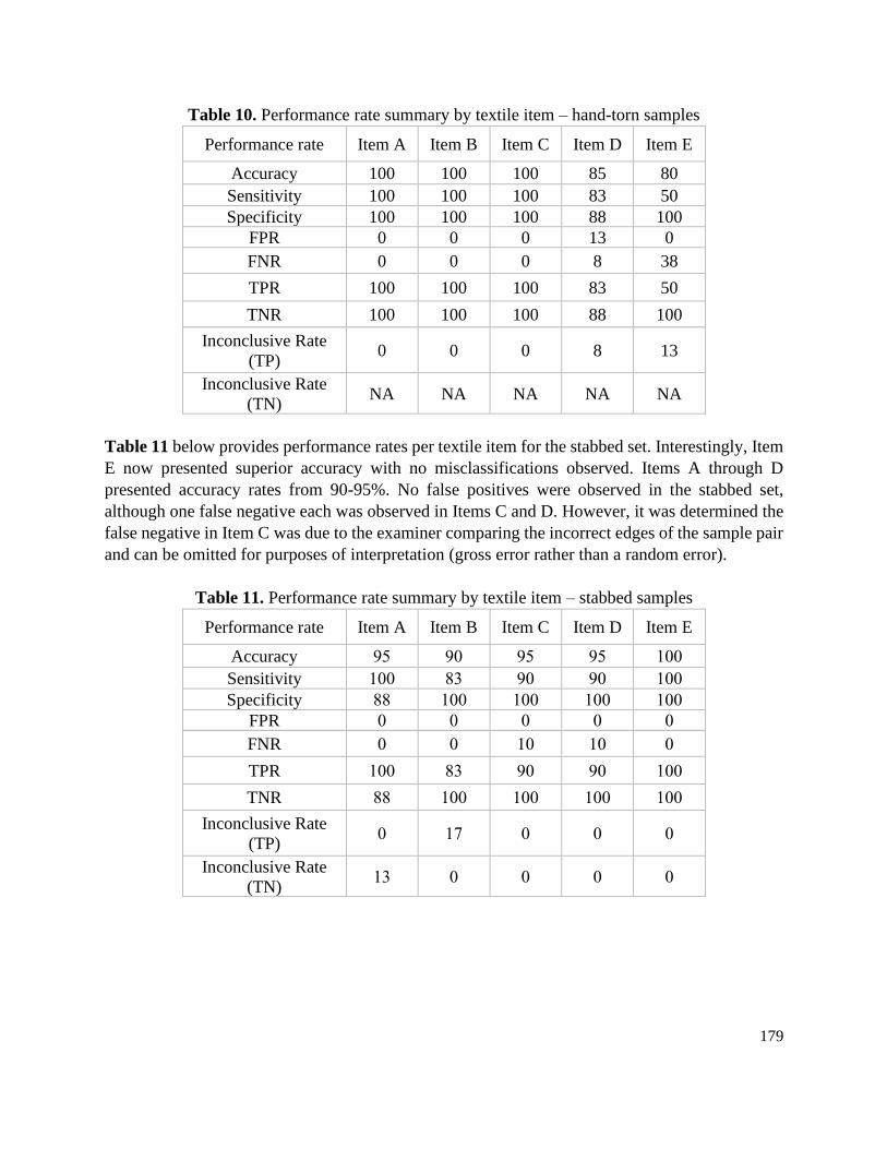
179
Table 10. Performance rate summary by textile item – hand-torn samples
Performance rate Item A Item B Item C Item D Item E
Accuracy 100 100 100 85 80
Sensitivity 100 100 100 83 50
Specificity 100 100 100 88 100
FPR 0 0 0 13 0
FNR 0 0 0 8 38
TPR 100 100 100 83 50
TNR 100 100 100 88 100
Inconclusive Rate
(TP) 0 0 0 8 13
Inconclusive Rate
(TN) NA NA NA NA NA
Table 11 below provides performance rates per textile item for the stabbed set. Interestingly, Item
E now presented superior accuracy with no misclassifications observed. Items A through D
presented accuracy rates from 90-95%. No false positives were observed in the stabbed set,
although one false negative each was observed in Items C and D. However, it was determined the
false negative in Item C was due to the examiner comparing the incorrect edges of the sample pair
and can be omitted for purposes of interpretation (gross error rather than a random error).
Table 11. Performance rate summary by textile item – stabbed samples
Performance rate Item A Item B Item C Item D Item E
Accuracy 95 90 95 95 100
Sensitivity 100 83 90 90 100
Specificity 88 100 100 100 100
FPR 0 0 0 0 0
FNR 0 0 10 10 0
TPR 100 83 90 90 100
TNR 88 100 100 100 100
Inconclusive Rate
(TP) 0 17 0 0 0
Inconclusive Rate
(TN) 13 0 0 0 0
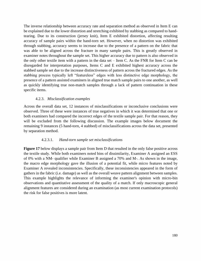
180
The inverse relationship between accuracy rate and separation method as observed in Item E can
be explained due to the lower distortion and stretching exhibited by stabbing as compared to hand-
tearing. Due to its construction (jersey knit), Item E exhibited distortion, affecting resulting
accuracy of sample pairs within the hand-torn set. However, when no distortion was exhibited
through stabbing, accuracy seems to increase due to the presence of a pattern on the fabric that
was able to be aligned across the fracture in many sample pairs. This is greatly observed in
examiner notes throughout the sample set. This higher accuracy due to pattern is also observed in
the only other textile item with a pattern in the data set – Item C. As the FNR for Item C can be
disregarded for interpretation purposes, Items C and E exhibited highest accuracy across the
stabbed sample set due to the increase distinctiveness of pattern across the fractured edges. As the
stabbing process typically left “featureless” edges with less distinctive edge morphology, the
presence of a pattern assisted examiners in aligned true match sample pairs to one another, as well
as quickly identifying true non-match samples through a lack of pattern continuation in these
specific items.
4.2.3. Misclassification examples
Across the overall data set, 12 instances of misclassifications or inconclusive conclusions were
observed. Three of these were instances of true negatives in which it was determined that one or
both examiners had compared the incorrect edges of the textile sample pair. For that reason, they
will be excluded from the following discussion. The example images below document the
remaining 9 instances (5 hand-torn, 4 stabbed) of misclassifications across the data set, presented
by separation method.
4.2.3.1. Hand-torn sample set misclassifications
Figure 17 below displays a sample pair from Item D that resulted in the only false positive across
the textile study. While both examiners noted bins of dissimilarity, Examiner A assigned an ESS
of 0% with a NM- qualifier while Examiner B assigned a 70% and M-. As shown in the image,
the macro edge morphology gave the illusion of a potential fit, while micro features noted by
Examiner A revealed inconsistencies. Specifically, these inconsistencies appeared in the form of
gathers in the fabric (i.e. damage) as well as the overall weave pattern alignment between samples.
This example highlights the relevance of informing the examiner's opinion with micro-bin
observations and quantitative assessment of the quality of a match. If only macroscopic general
alignment features are considered during an examination (as most current examination protocols)
the risk for false positives is more latent.
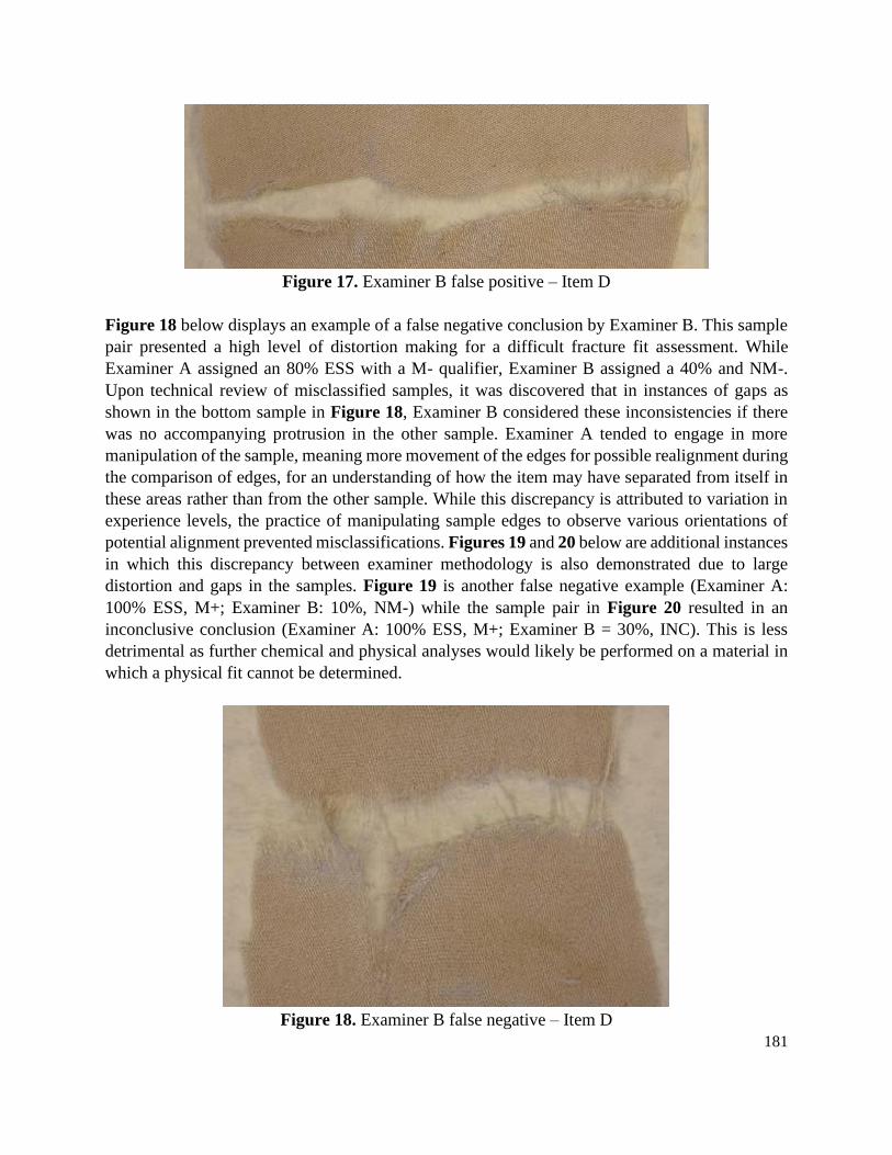
181
Figure 17. Examiner B false positive – Item D
Figure 18 below displays an example of a false negative conclusion by Examiner B. This sample
pair presented a high level of distortion making for a difficult fracture fit assessment. While
Examiner A assigned an 80% ESS with a M- qualifier, Examiner B assigned a 40% and NM-.
Upon technical review of misclassified samples, it was discovered that in instances of gaps as
shown in the bottom sample in Figure 18, Examiner B considered these inconsistencies if there
was no accompanying protrusion in the other sample. Examiner A tended to engage in more
manipulation of the sample, meaning more movement of the edges for possible realignment during
the comparison of edges, for an understanding of how the item may have separated from itself in
these areas rather than from the other sample. While this discrepancy is attributed to variation in
experience levels, the practice of manipulating sample edges to observe various orientations of
potential alignment prevented misclassifications. Figures 19 and 20 below are additional instances
in which this discrepancy between examiner methodology is also demonstrated due to large
distortion and gaps in the samples. Figure 19 is another false negative example (Examiner A:
100% ESS, M+; Examiner B: 10%, NM-) while the sample pair in Figure 20 resulted in an
inconclusive conclusion (Examiner A: 100% ESS, M+; Examiner B = 30%, INC). This is less
detrimental as further chemical and physical analyses would likely be performed on a material in
which a physical fit cannot be determined.
Figure 18. Examiner B false negative – Item D
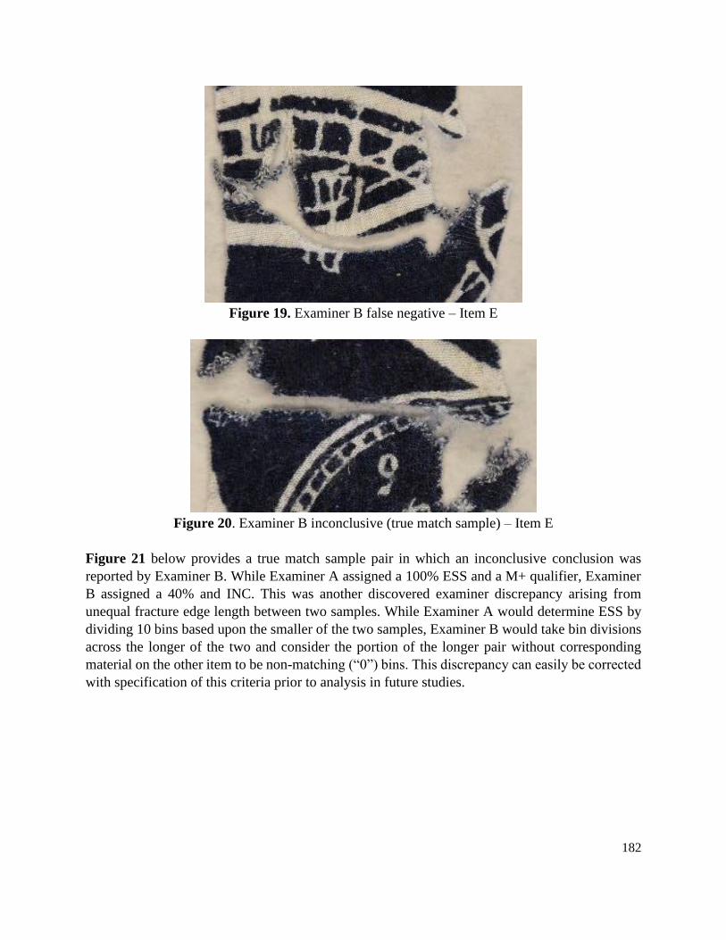
182
Figure 19. Examiner B false negative – Item E
Figure 20. Examiner B inconclusive (true match sample) – Item E
Figure 21 below provides a true match sample pair in which an inconclusive conclusion was
reported by Examiner B. While Examiner A assigned a 100% ESS and a M+ qualifier, Examiner
B assigned a 40% and INC. This was another discovered examiner discrepancy arising from
unequal fracture edge length between two samples. While Examiner A would determine ESS by
dividing 10 bins based upon the smaller of the two samples, Examiner B would take bin divisions
across the longer of the two and consider the portion of the longer pair without corresponding
material on the other item to be non-matching (“0”) bins. This discrepancy can easily be corrected
with specification of this criteria prior to analysis in future studies.
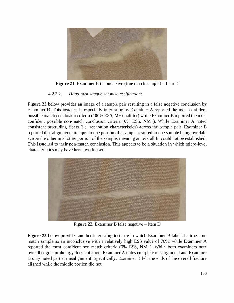
183
Figure 21. Examiner B inconclusive (true match sample) – Item D
4.2.3.2. Hand-torn sample set misclassifications
Figure 22 below provides an image of a sample pair resulting in a false negative conclusion by
Examiner B. This instance is especially interesting as Examiner A reported the most confident
possible match conclusion criteria (100% ESS, M+ qualifier) while Examiner B reported the most
confident possible non-match conclusion criteria (0% ESS, NM+). While Examiner A noted
consistent protruding fibers (i.e. separation characteristics) across the sample pair, Examiner B
reported that alignment attempts in one portion of a sample resulted in one sample being overlaid
across the other in another portion of the sample, meaning an overall fit could not be established.
This issue led to their non-match conclusion. This appears to be a situation in which micro-level
characteristics may have been overlooked.
Figure 22. Examiner B false negative – Item D
Figure 23 below provides another interesting instance in which Examiner B labeled a true non-
match sample as an inconclusive with a relatively high ESS value of 70%, while Examiner A
reported the most confident non-match criteria (0% ESS, NM+). While both examiners note
overall edge morphology does not align, Examiner A notes complete misalignment and Examiner
B only noted partial misalignment. Specifically, Examiner B felt the ends of the overall fracture
aligned while the middle portion did not.
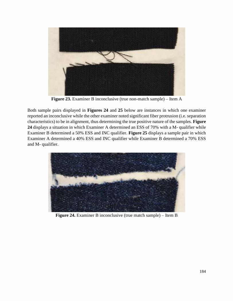
184
Figure 23. Examiner B inconclusive (true non-match sample) – Item A
Both sample pairs displayed in Figures 24 and 25 below are instances in which one examiner
reported an inconclusive while the other examiner noted significant fiber protrusion (i.e. separation
characteristics) to be in alignment, thus determining the true positive nature of the samples. Figure
24 displays a situation in which Examiner A determined an ESS of 70% with a M- qualifier while
Examiner B determined a 50% ESS and INC qualifier. Figure 25 displays a sample pair in which
Examiner A determined a 40% ESS and INC qualifier while Examiner B determined a 70% ESS
and M- qualifier.
Figure 24. Examiner B inconclusive (true match sample) – Item B
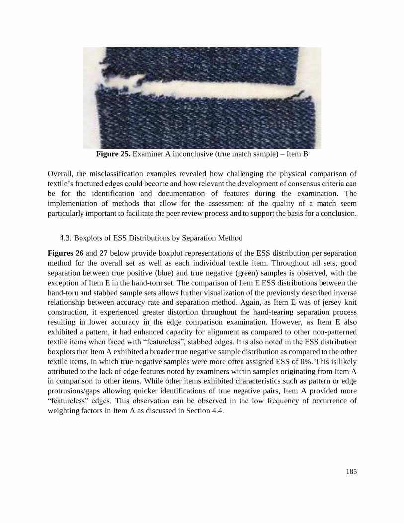
185
Figure 25. Examiner A inconclusive (true match sample) – Item B
Overall, the misclassification examples revealed how challenging the physical comparison of
textile’s fractured edges could become and how relevant the development of consensus criteria can
be for the identification and documentation of features during the examination. The
implementation of methods that allow for the assessment of the quality of a match seem
particularly important to facilitate the peer review process and to support the basis for a conclusion.
4.3. Boxplots of ESS Distributions by Separation Method
Figures 26 and 27 below provide boxplot representations of the ESS distribution per separation
method for the overall set as well as each individual textile item. Throughout all sets, good
separation between true positive (blue) and true negative (green) samples is observed, with the
exception of Item E in the hand-torn set. The comparison of Item E ESS distributions between the
hand-torn and stabbed sample sets allows further visualization of the previously described inverse
relationship between accuracy rate and separation method. Again, as Item E was of jersey knit
construction, it experienced greater distortion throughout the hand-tearing separation process
resulting in lower accuracy in the edge comparison examination. However, as Item E also
exhibited a pattern, it had enhanced capacity for alignment as compared to other non-patterned
textile items when faced with “featureless”, stabbed edges. It is also noted in the ESS distribution
boxplots that Item A exhibited a broader true negative sample distribution as compared to the other
textile items, in which true negative samples were more often assigned ESS of 0%. This is likely
attributed to the lack of edge features noted by examiners within samples originating from Item A
in comparison to other items. While other items exhibited characteristics such as pattern or edge
protrusions/gaps allowing quicker identifications of true negative pairs, Item A provided more
“featureless” edges. This observation can be observed in the low frequency of occurrence of
weighting factors in Item A as discussed in Section 4.4.
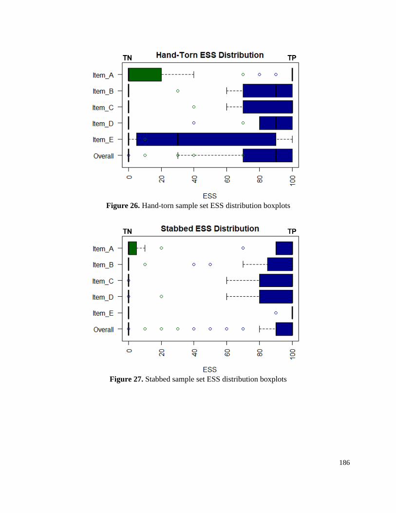
186
Figure 26. Hand-torn sample set ESS distribution boxplots
Figure 27. Stabbed sample set ESS distribution boxplots
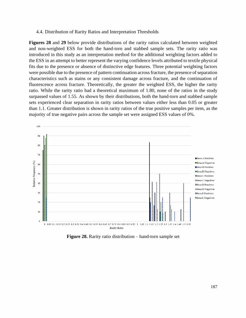
187
4.4. Distribution of Rarity Ratios and Interpretation Thresholds
Figures 28 and 29 below provide distributions of the rarity ratios calculated between weighted
and non-weighted ESS for both the hand-torn and stabbed sample sets. The rarity ratio was
introduced in this study as an interpretation method for the additional weighting factors added to
the ESS in an attempt to better represent the varying confidence levels attributed to textile physical
fits due to the presence or absence of distinctive edge features. Three potential weighting factors
were possible due to the presence of pattern continuation across fracture, the presence of separation
characteristics such as stains or any consistent damage across fracture, and the continuation of
fluorescence across fracture. Theoretically, the greater the weighted ESS, the higher the rarity
ratio. While the rarity ratio had a theoretical maximum of 1.80, none of the ratios in the study
surpassed values of 1.55. As shown by their distributions, both the hand-torn and stabbed sample
sets experienced clear separation in rarity ratios between values either less than 0.05 or greater
than 1.1. Greater distribution is shown in rarity ratios of the true positive samples per item, as the
majority of true negative pairs across the sample set were assigned ESS values of 0%.
Figure 28. Rarity ratio distribution – hand-torn sample set
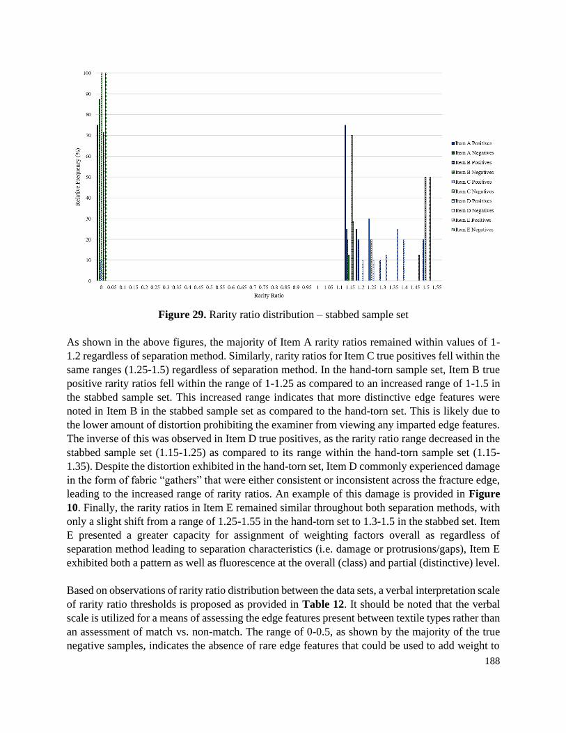
188
Figure 29. Rarity ratio distribution – stabbed sample set
As shown in the above figures, the majority of Item A rarity ratios remained within values of 1-
1.2 regardless of separation method. Similarly, rarity ratios for Item C true positives fell within the
same ranges (1.25-1.5) regardless of separation method. In the hand-torn sample set, Item B true
positive rarity ratios fell within the range of 1-1.25 as compared to an increased range of 1-1.5 in
the stabbed sample set. This increased range indicates that more distinctive edge features were
noted in Item B in the stabbed sample set as compared to the hand-torn set. This is likely due to
the lower amount of distortion prohibiting the examiner from viewing any imparted edge features.
The inverse of this was observed in Item D true positives, as the rarity ratio range decreased in the
stabbed sample set (1.15-1.25) as compared to its range within the hand-torn sample set (1.15-
1.35). Despite the distortion exhibited in the hand-torn set, Item D commonly experienced damage
in the form of fabric “gathers” that were either consistent or inconsistent across the fracture edge,
leading to the increased range of rarity ratios. An example of this damage is provided in Figure
10. Finally, the rarity ratios in Item E remained similar throughout both separation methods, with
only a slight shift from a range of 1.25-1.55 in the hand-torn set to 1.3-1.5 in the stabbed set. Item
E presented a greater capacity for assignment of weighting factors overall as regardless of
separation method leading to separation characteristics (i.e. damage or protrusions/gaps), Item E
exhibited both a pattern as well as fluorescence at the overall (class) and partial (distinctive) level.
Based on observations of rarity ratio distribution between the data sets, a verbal interpretation scale
of rarity ratio thresholds is proposed as provided in Table 12. It should be noted that the verbal
scale is utilized for a means of assessing the edge features present between textile types rather than
an assessment of match vs. non-match. The range of 0-0.5, as shown by the majority of the true
negative samples, indicates the absence of rare edge features that could be used to add weight to
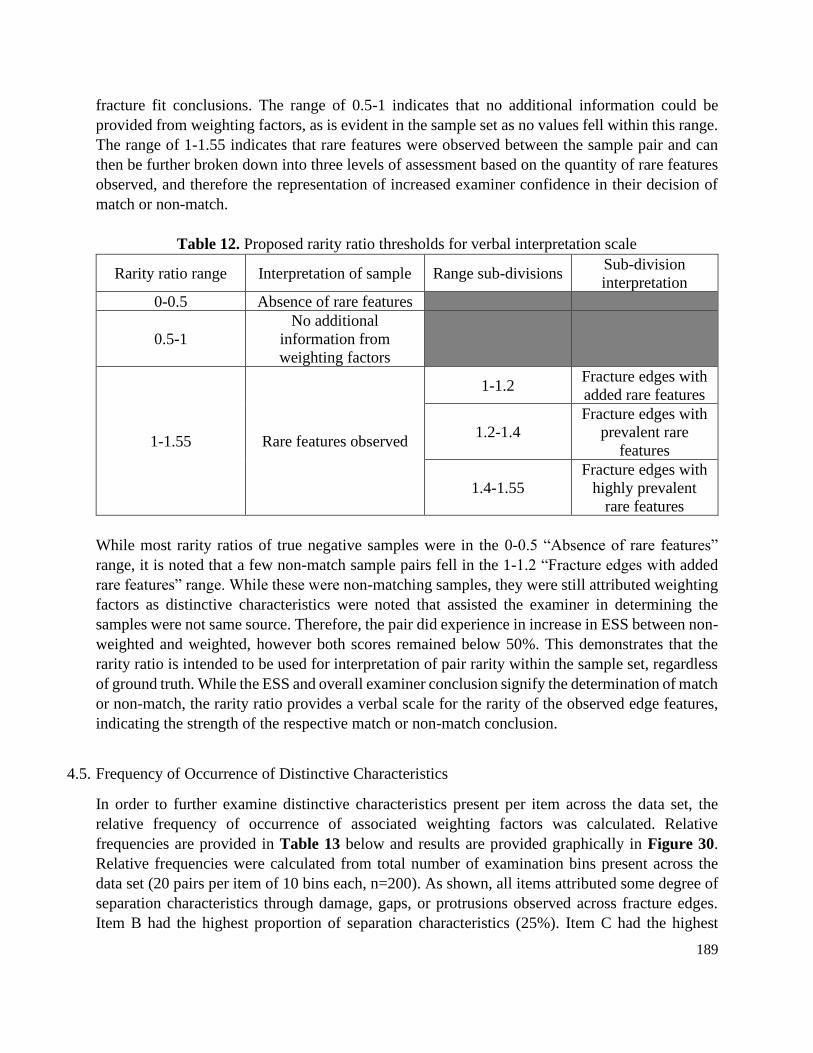
189
fracture fit conclusions. The range of 0.5-1 indicates that no additional information could be
provided from weighting factors, as is evident in the sample set as no values fell within this range.
The range of 1-1.55 indicates that rare features were observed between the sample pair and can
then be further broken down into three levels of assessment based on the quantity of rare features
observed, and therefore the representation of increased examiner confidence in their decision of
match or non-match.
Table 12. Proposed rarity ratio thresholds for verbal interpretation scale
Rarity ratio range Interpretation of sample Range sub-divisions Sub-division
interpretation
0-0.5 Absence of rare features
0.5-1
No additional
information from
weighting factors
1-1.55 Rare features observed
1-1.2 Fracture edges with
added rare features
1.2-1.4
Fracture edges with
prevalent rare
features
1.4-1.55
Fracture edges with
highly prevalent
rare features
While most rarity ratios of true negative samples were in the 0-0.5 “Absence of rare features”
range, it is noted that a few non-match sample pairs fell in the 1-1.2 “Fracture edges with added
rare features” range. While these were non-matching samples, they were still attributed weighting
factors as distinctive characteristics were noted that assisted the examiner in determining the
samples were not same source. Therefore, the pair did experience in increase in ESS between non-
weighted and weighted, however both scores remained below 50%. This demonstrates that the
rarity ratio is intended to be used for interpretation of pair rarity within the sample set, regardless
of ground truth. While the ESS and overall examiner conclusion signify the determination of match
or non-match, the rarity ratio provides a verbal scale for the rarity of the observed edge features,
indicating the strength of the respective match or non-match conclusion.
4.5. Frequency of Occurrence of Distinctive Characteristics
In order to further examine distinctive characteristics present per item across the data set, the
relative frequency of occurrence of associated weighting factors was calculated. Relative
frequencies are provided in Table 13 below and results are provided graphically in Figure 30.
Relative frequencies were calculated from total number of examination bins present across the
data set (20 pairs per item of 10 bins each, n=200). As shown, all items attributed some degree of
separation characteristics through damage, gaps, or protrusions observed across fracture edges.
Item B had the highest proportion of separation characteristics (25%). Item C had the highest
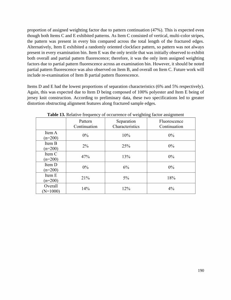
190
proportion of assigned weighting factor due to pattern continuation (47%). This is expected even
though both Items C and E exhibited patterns. As Item C consisted of vertical, multi-color stripes,
the pattern was present in every bin compared across the total length of the fractured edges.
Alternatively, Item E exhibited a randomly oriented clockface pattern, so pattern was not always
present in every examination bin. Item E was the only textile that was initially observed to exhibit
both overall and partial pattern fluorescence; therefore, it was the only item assigned weighting
factors due to partial pattern fluorescence across an examination bin. However, it should be noted
partial pattern fluorescence was also observed on Item B, and overall on Item C. Future work will
include re-examination of Item B partial pattern fluorescence.
Items D and E had the lowest proportions of separation characteristics (6% and 5% respectively).
Again, this was expected due to Item D being composed of 100% polyester and Item E being of
jersey knit construction. According to preliminary data, these two specifications led to greater
distortion obstructing alignment features along fractured sample edges.
Table 13. Relative frequency of occurrence of weighting factor assignment
Pattern
Continuation
Separation
Characteristics
Fluorescence
Continuation
Item A
(n=200) 0% 10% 0%
Item B
(n=200) 2% 25% 0%
Item C
(n=200) 47% 13% 0%
Item D
(n=200) 0% 6% 0%
Item E
(n=200) 21% 5% 18%
Overall
(N=1000) 14% 12% 4%
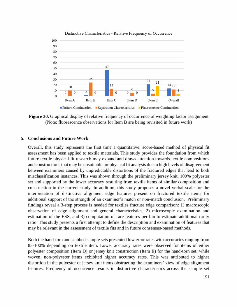
191
Figure 30. Graphical display of relative frequency of occurrence of weighting factor assignment
(Note: fluorescence observations for Item B are being revisited in future work)
5. Conclusions and Future Work
Overall, this study represents the first time a quantitative, score-based method of physical fit
assessment has been applied to textile materials. This study provides the foundation from which
future textile physical fit research may expand and draws attention towards textile compositions
and constructions that may be unsuitable for physical fit analysis due to high levels of disagreement
between examiners caused by unpredictable distortions of the fractured edges that lead to both
misclassification instances. This was shown through the preliminary jersey knit, 100% polyester
set and supported by the lower accuracy resulting from textile items of similar composition and
construction in the current study. In addition, this study proposes a novel verbal scale for the
interpretation of distinctive alignment edge features present on fractured textile items for
additional support of the strength of an examiner’s match or non-match conclusion. Preliminary
findings reveal a 3-step process is needed for textiles fracture edge comparison: 1) macroscopic
observation of edge alignment and general characteristics, 2) microscopic examination and
estimation of the ESS, and 3) computation of rare features per bin to estimate additional rarity
ratio. This study presents a first attempt to define the description and examination of features that
may be relevant in the assessment of textile fits and in future consensus-based methods.
Both the hand-torn and stabbed sample sets presented low error rates with accuracies ranging from
85-100% depending on textile item. Lower accuracy rates were observed for items of either
polyester composition (Item D) or jersey knit construction (Item E) for the hand-torn set, while
woven, non-polyester items exhibited higher accuracy rates. This was attributed to higher
distortion in the polyester or jersey knit items obstructing the examiners’ view of edge alignment
features. Frequency of occurrence results in distinctive characteristics across the sample set
192
support this, as woven materials tended to exhibit a greater percentage of separation characteristics
than other materials. For the stabbed sample set, it was observed that patterned materials (Items C
and E) exhibited higher accuracy rates than solid-colored items. This was attributed to the added
potential of pattern alignment (or misalignment) on items presenting otherwise “featureless” edges
due to the stabbing separation mechanism.
Further analysis of examiner notes revealed two main methodology discrepancies dealing with
treatment of gaps within a sample as well as inconsistent fracture edge length between two items.
While Examiner A tended to manipulate samples to gain an understanding if gaps were due to an
item separating from itself rather than another item, Examiner B treated these gaps as
inconsistencies between the pair if the other item did not have a corresponding protrusion. In
addition, Examiner A tended to take bin divisions from the smaller fracture edge length of two
compared items while Examiner B tended to take bin divisions from the larger of the two. Both of
these methodology discrepancies may be alleviated through further examiner training and specific
distinction of bin division criteria prior to sample analysis, which may be implemented in a future
study. Regardless of examiner discrepancies, only 12 misclassifications were observed across the
entire data set. Only one of these was a false positive, with the remainder consisted of false
negatives and inconclusive conclusions (not true misclassifications). These results are less
detrimental to casework as negative or inconclusive samples would typically be taken through
further physical and chemical analysis in a forensic laboratory.
This study represents a successful first expansion of the previously developed duct tape physical
fit ESS methodology to an additional material. The results highlighted the relevance of
development of material-specific approaches, as the factors that influence the quality of a match
and error rates varied widely between duct tapes and textiles. Future work will include studies of
expanded textile factors such as additional compositions, constructions, and external factors such
as degree of wear. This work will identify any needed modifications to the ESS method to best
account for additional encountered separation characteristics due to fabric type. Expanded work
and increased sample sets will also assist in the fine-tuning of the proposed verbal interpretation
based upon rarity ratio thresholds. Finally, an inter-laboratory study will be initiated to validate
the now developed textile ESS methodology.
6. References
1. Grieve M, Houck MM. Introduction. In: Houck MM, editor. Trace Evidence Analysis: More
Cases in Mute Witnesses. Burlington, MA: ElSevier Academic Press; 2004. p. 1–26.
2. Fisher BAJ, Svensson A, Wendel O. Techniques of Crime Scene Investigation. 4th ed. Fisher
BAJ, editor. New York, NY: Elsevier Science Publishing Co., Inc.; 1987.
3. Shor Y, Novoselsky Y, Klein A, Lurie DJ, Levi JA, Vinokurov A, Levin N. The Identification
of Stolen Paintings Using Comparison of Various Marks. Journal of Forensic Sciences. 2002:633–
637.
193
4. Gross S. NIST-OSAC Materials (Trace) Subcommittee, physical fit task group, 2020 physical
fit survey.
5. Dann T, Malbon C. Tearing or Ripping of Fabrics. In: Carr D, editor. Forensic Textile Science.
Cambridge, MA: Woodhead Publishing; 2017. p. 169–180.
6. Kemp SE, Carr DJ, Kieser J, Niven BE, Taylor MC. Forensic evidence in apparel fabrics due to
stab events. Forensic Science International. 2009;191:86–96. doi:10.1016/j.forsciint.2009.06.013
7. Pelton WR. Distinguishing the Cause of Textile Fiber Damage Using the Scanning Electron
Microscope (SEM). Journal of Forensic Sciences. 1995;40(5):874–882.
8. Brooks E, Prusinowski M, Gross S, Trejos T. Forensic physical fits in the trace evidence
discipline: A review. Forensic Science International. 2020. doi:10.1016/j.biteb.2019.100321
9. Prusinowski M, Brooks E, Trejos T. Development and validation of a systematic approach for
the quantitative assessment of the quality of duct tape physical fits. Forensic Science International.
2020;307.
194
V. CHAPTER FOUR
Optimization and Evaluation of Spectral Comparisons of Electrical Tape
Backings by X-ray Fluorescence
Abstract:
Electrical tape can be relevant forensic evidence in high-profile casework involving shootings or
explosive devices. It is critical that practitioners have access to rapid, informative, and minimally
invasive techniques of analysis to best support these investigations. The characterization of
electrical tape backings through X-ray Fluorescence (XRF) Spectroscopy has been shown to be a
highly discriminatory, non-destructive method of analysis requiring limited sample preparation.
This study describes the process of parameter optimization of an XRF method for casework use.
The work expands upon previous discrimination studies by broadening the total sample set of
characterized tapes and evaluating the use of spectral overlay, spectral contrast angle, and
Quadratic Discriminant Analysis (QDA) for the comparison of XRF spectra. The expanded sample
set consisted of 114 samples, 94 from different sources of which 90 were previously analyzed, and
20 from the same roll. For each sample, replicate measurements on different locations of the tape
were analyzed (n=3) to assess the intra-roll variability. XRF provided superior discrimination to
Scanning Electron Microscopy with Energy Dispersive Spectroscopy (SEM-EDS) on the
expanded dataset and a more comprehensive elemental characterization (15 elements by XRF vs.
8 by SEM-EDS). While previous SEM-EDS analysis of the 90 electrical tapes resulted in 15
distinct groups and a discrimination power of 87.3%, current XRF analysis considering the
equivalent 90 electrical tapes resulted in 61 distinct groups with further subgroups providing a
discrimination power of 96.7%.
Duplicate controls and tape fragments from the same roll were also analyzed to assess inter-day,
intra-day, and intra-roll variability (n=20). Parameter optimization included comparison of
atmospheric conditions, collection times, and instrumental filters. A study of the effects of
adhesive and backing thickness on spectrum collection revealed key implications to the method
that required modification to the sample support material. As an electrical tape standard reference
material does not currently exist, NIST SRM 1831, a standard soda-lime glass, was found to be an
adequate reference material for daily performance assessment of the instrument.
In addition, figures of merit assessed included accuracy and discrimination over time, precision,
sensitivity, and selectivity. The performance of different methods for comparing and contrasting
spectra was also evaluated. The optimization of this method was part of an assessment to
incorporate XRF to a forensic laboratory protocol for rapid, highly informative elemental analysis
of electrical tape backings and to expand examiners’ casework capabilities.
1. Introduction
Pressure-sensitive tapes are often involved in the commission of a crime due to their low cost, ease
of use, and their readily available nature. Specifically, electrical tape is commonly submitted to
forensic laboratories in reference to crimes such as shootings (e.g., tape used for modifications to
195
weapons) or bombing events (e.g., tape remaining from an improvised explosive device). It is
critical that forensic scientists have access to rapid, highly discriminatory techniques to best utilize
the potential of this type of physical evidence.
In a typical analytical scheme for electrical tape comparative analysis, examinations begin with
physical characteristics and continue to chemical analysis if a discrimination is not made between
items. Examination of physical characteristics includes documentation of color and thickness of
respective backing and adhesive layers, as well as the overall width and surface texture.1 A full
analytical scheme also consists of a combination of chemical and elemental techniques to provide
a comprehensive characterization of all components of a tape sample. All-encompassing analytical
schemes for electrical tapes are well-established in the literature.1–7
Electrical tape is composed of a backing and adhesive layer. Backing components can include the
main polymer, plasticizers, fillers, pigments, flame retardants, stabilizers, and lubricants. The most
common polymer used for electrical tape backings is polyvinyl chloride (PVC), but other polymers
such as polyethylene, polypropylene, polyester, and polyimide are also used.3,4 Plasticizers are
often added to soften the polymer to provide flexibility to the tape backing. These include aromatic
plasticizers such as dialkyl phthalate esters or trialkyl trimellitate esters, or aliphatic plasticizers
such as dialkyl adipate esters or tricresyl phosphates.6 Other components such as carbon black,
calcium carbonate, titanium dioxide, barium sulfate, kaolin, talc, and dolomite are used as
opacifiers, colorants and fillers.4,6 Flame retardants reduce the flammability of electrical tape due
to the added plasticizers. Some common flame retardants include antimony oxide and aluminum
hydroxide.6 Stabilizers, such as lead carbonate and lead sulfate, are added to prevent
decomposition or ultraviolet irradiation degradation.6 Finally, adhesive components include a base
elastomer (e.g., polyisoprene, polybutadiene), copolymers [e.g., poly(styrene-co-isoprene) or
poly(styrene-co-butadiene), and poly(butylacrylate], and tackifying resins (e.g., wood rosin,
terpene resins, and petroleum resins), along with aromatic and/or aliphatic plasticizers,
antioxidants, flame retardants, and fillers.4,6
Chemical analysis techniques vary depending upon the availability of the instruments and
associated sample size. For example, Fourier-Transform Infrared Spectroscopy (FTIR) is a non-
destructive method that reveals information on organic and some inorganic components of a tape
sample, while Pyrolysis Gas Chromatography/Mass Spectrometry (py-GC/MS) can provide
further characterization of the polymeric components. However, if there is a desire to preserve an
evidence item of limited size, py-GC/MS may not be utilized as it is a destructive method.5
Elemental methods are used to characterize the inorganic components of the tape sample such as
stabilizers, flame retardants, and fillers.6 Common methodology for electrical tapes includes
Scanning Electron Microscopy with Energy Dispersive X-Ray Spectroscopy (SEM-EDS),3 which
provides both an elemental profile of the sample and a topographic image of the scanned surface.5,6
This traditional analytical scheme was employed in a previous study by Mehltretter et al.4 in which
a set of 90 black electrical tapes was characterized by the physical and chemical characteristics of
their backings. Physical examination resulted in a discrimination power of 64%, while FTIR, py-
GC/MS, and SEM-EDS analyses resulted in discrimination powers of 83%, 81%, and 87%,
respectively. Considering the overall analytical scheme of the tape backings, the authors achieved
196
94% discrimination.4 Combining the adhesive with the backing results for the same sample set,
the discrimination was raised to 96%.3
While high discrimination was achieved in the Mehltretter studies,3,4 a full analytical scheme for
both the adhesive and backing of all tape samples was required. Additional research has reported
on rapid techniques that are able to achieve high discrimination as a screening method to
complement conventional analytical schemes such as X-ray Fluorescence Spectroscopy (XRF)8–
10 and Laser Ablation - Inductively Coupled Plasma – Mass Spectrometry (LA-ICP-MS).11,12 Of
these methods, XRF is easier to operate, non-destructive, and more widely available in forensic
laboratories.
X-ray Fluorescence (XRF) Spectroscopy utilizes an X-ray beam to initiate photoelectric absorption
in atoms present in the sample. This energy absorption occurs if the energy of the X-ray photons
irradiating the sample is larger than the binding energy of the inner electron orbitals of a given
atom, and results in inelastic ejection of an electron from its inner shells within the orbital. As an
outer orbital electron transfers to fill this vacancy to restore the system stability, an X-ray photon
is produced with an energy equivalent to the energy difference between the initial and final
quantum states of the electron. Characteristic X-ray emission lines correspond to peaks within the
resulting spectrum that can be used to identify the elemental composition of the sample in
question.13
XRF was previously utilized by Kee in the characterization of 131 black PVC electrical tape
backing samples obtained through casework from 1980 to 1981. One-centimeter length tape
segments were cut from respective rolls. Their backings were wiped with hexane prior to analysis,
and samples were mounted on Mylar film held by a plastic sample cup. Only the top surface of the
tape backing was analyzed. Four major classes were identified due to the presence or absence of
lead and calcium, with further discrimination into 15 subclasses due to the presence of additional
phosphorus, antimony, silicon, sulfur, and titanium.8 XRF analysis was also utilized in a study by
Keto in which two rolls each of six tape brands were characterized according to the presence or
absence of ten elements: aluminum, silicon, sulfur, chlorine, antimony, calcium, titanium, iron,
zinc, and lead. Means and standard deviations of resulting counts were assessed to determine low
within-brand variability and sufficient variability between brands to allow for discrimination.9
In a previous study by Prusinowski et al., the authors utilized three different XRF instrumental
configurations to compare discrimination power when characterizing a set of 40 electrical tape
backings.10 The results were compared to those of previous studies examining the same set of
electrical tapes.4,11 XRF was found to be comparable to LA-ICP-MS when considering N=40
overall samples, with the most sensitive XRF configuration achieving a discrimination power of
90.1% as opposed to LA-ICP-MS at 84.6%. The difference in discrimination power was noted to
likely be a result of the presence of iron in the XRF spectra, whereas iron can be difficult to detect
on standard quadrupole LA-ICP-MS instruments due to common polyatomic interferences. The
enhanced discrimination by XRF was also attributed to an instrumental configuration with a larger
spot size (e.g., 1 cm vs. 100-300 µm). In addition, the Prusinowski study10 evaluated a semi-
quantitative method to compare samples. The relative area under the relevant elemental peaks in
the XRF spectra was calculated and compared using Analysis of Variance (ANOVA) to determine
which sample signal-to-noise ratios (SNRs) were significantly different.10
197
The aim of the current study was to evaluate the XRF method for use within a forensic laboratory
by optimizing each selected parameter including atmospheric condition, collection time, sample
support material, filters used, adhesive effects, and backing thickness effects. Further
experimentation was then performed utilizing optimized parameters for assessments of accuracy
and discrimination over time, precision, sensitivity, and selectivity. In addition, the previous
sample set of 40 electrical tapes10 was increased to a full characterization of 94 samples originating
from different-product rolls as well as an intra-roll variability study consisting of 20 same roll
samples.
Following data collection, data analyses performed included spectral overlay comparison,
estimation of spectral contrast angle ratios, and Quadratic Discriminant Analysis (QDA).
Spectral overlay and contrast angle comparison methods are useful for determining if respective
XRF spectra demonstrate two tape samples originated from different sources. Likewise, a spectral
comparison is informative in determining if two samples known to originate from the same source
(e.g., same roll) produce indistinguishable spectra. When the ground truth of sample origin is
known, these methods can be applied to evaluate false positives, false negatives, and accuracy.
When the source of the sample is unknown, as in casework, the comparison methods serve to
inform the examiner's opinion about whether or not the samples of interest could have originated
from a common source.
During XRF spectral overlay comparisons, the spectra are superimposed to determine if the
observed variability within the same source (i.e., replicate spectra of the known tape and replicate
spectra of the questioned sample) is smaller than the variability between the compared items (e.g.,
spectra of known versus questioned tape). The variability of XRF spectra is assessed by differences
of spectral shape or location (x-axis) and differences in the relative intensity of the peaks (y-axis).
When those spectral differences between the compared samples are outside the variability of
spectra originating from the same source, the samples are distinguished. Spectral overlay is a fast
and intuitive method of comparison that provides simple distinction of large differences between
samples. The method is widely used in forensic science and in spectrochemical comparisons in
general.
However, when the compared spectra are similar and differences between samples are much
smaller (i.e., a peak intensity (y-axis) difference only and no peak shape/location (x-axis)
differences), it becomes more difficult for the examiner to determine if these differences are
sufficient to distinguish or associate two samples. As a result, there are several alternative methods
and software features that can aid in the quantitative and automated assessment of the similarities
and differences between spectra. In this study, we proposed to evaluate the use a well-known and
straightforward comparison method using spectral contrast angles to establish the level of
similarity among spectra. In this method, each XRF spectrum can be represented as a vector whose
length and orientation are determined by the peak energy (x-axis, keV) and intensities (y-axis,
counts) of the spectrum. Then, the angle between the vectors of the compared spectra is calculated.
The smaller the angle between the compared vectors, the more similar the spectra and vice versa.
For instance, if two identical spectra were compared, the respective vectors would superimpose
each other, resulting in a zero-degree angle. On the other hand, if two very different spectra were
compared, the known and questioned vectors could show a difference as large as a 90-degree
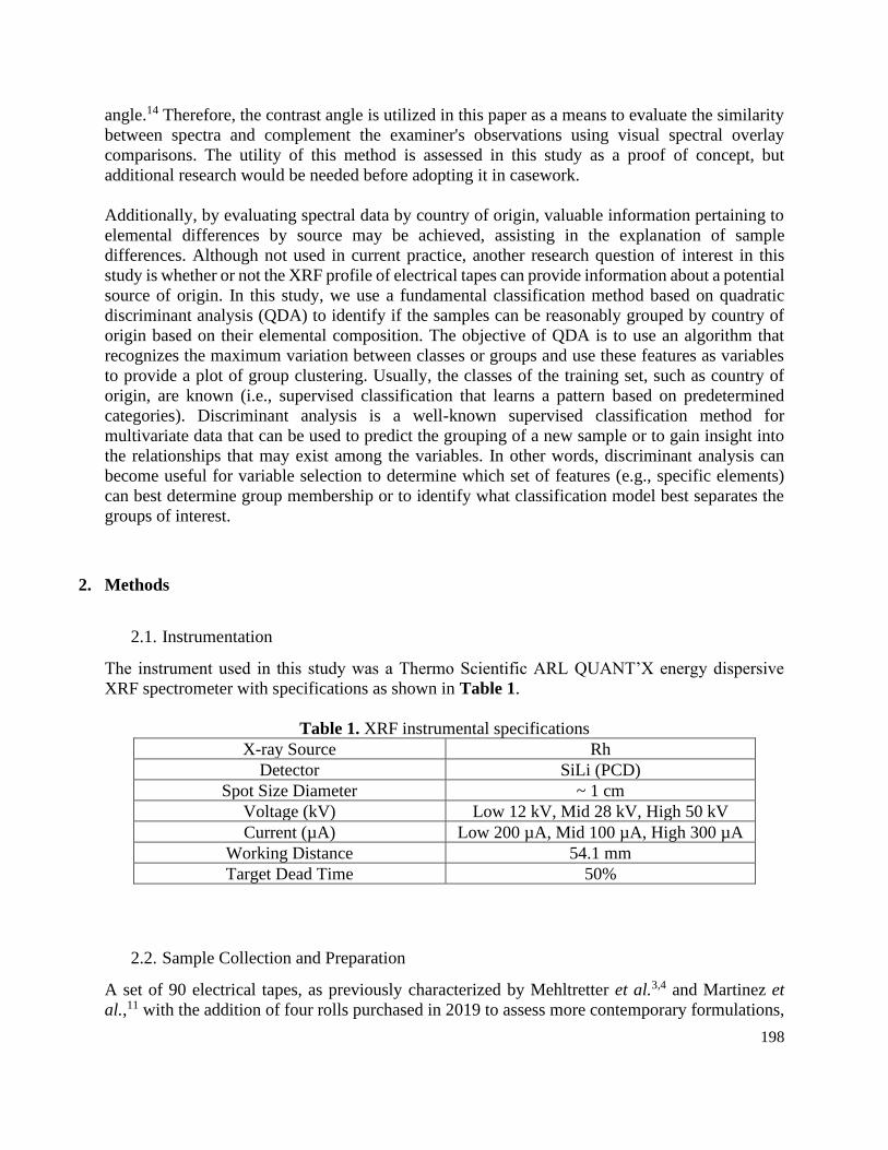
198
angle.14 Therefore, the contrast angle is utilized in this paper as a means to evaluate the similarity
between spectra and complement the examiner's observations using visual spectral overlay
comparisons. The utility of this method is assessed in this study as a proof of concept, but
additional research would be needed before adopting it in casework.
Additionally, by evaluating spectral data by country of origin, valuable information pertaining to
elemental differences by source may be achieved, assisting in the explanation of sample
differences. Although not used in current practice, another research question of interest in this
study is whether or not the XRF profile of electrical tapes can provide information about a potential
source of origin. In this study, we use a fundamental classification method based on quadratic
discriminant analysis (QDA) to identify if the samples can be reasonably grouped by country of
origin based on their elemental composition. The objective of QDA is to use an algorithm that
recognizes the maximum variation between classes or groups and use these features as variables
to provide a plot of group clustering. Usually, the classes of the training set, such as country of
origin, are known (i.e., supervised classification that learns a pattern based on predetermined
categories). Discriminant analysis is a well-known supervised classification method for
multivariate data that can be used to predict the grouping of a new sample or to gain insight into
the relationships that may exist among the variables. In other words, discriminant analysis can
become useful for variable selection to determine which set of features (e.g., specific elements)
can best determine group membership or to identify what classification model best separates the
groups of interest.
2. Methods
2.1. Instrumentation
The instrument used in this study was a Thermo Scientific ARL QUANT’X energy dispersive
XRF spectrometer with specifications as shown in Table 1.
Table 1. XRF instrumental specifications
X-ray Source Rh
Detector SiLi (PCD)
Spot Size Diameter ~ 1 cm
Voltage (kV) Low 12 kV, Mid 28 kV, High 50 kV
Current (µA) Low 200 µA, Mid 100 µA, High 300 µA
Working Distance 54.1 mm
Target Dead Time 50%
2.2. Sample Collection and Preparation
A set of 90 electrical tapes, as previously characterized by Mehltretter et al.3,4 and Martinez et
al.,11 with the addition of four rolls purchased in 2019 to assess more contemporary formulations,
199
was characterized with optimized XRF parameters. Product information for the expanded sample
set (N=94) is provided in Table A.1 of the Appendix.
Full width tape samples ~ 5-6 cm in length were cut from each roll. A sample size of at least 2 cm
in length was ideal to account for interaction of the detector aperture diameter with the tape.
However, smaller portions can be analyzed with the use of polypropylene or Mylar film, although
not assessed in this study. Adhesive was removed from the backing in a region ~ 2-3 cm in length
and across the full tape width to provide a large enough area for the ~1 cm beam diameter. This
becomes critical when attempting replicates of the same sample in various areas of the adhesive-
removed region. Adhesive removal took place with acetone or hexane. Samples were placed on
glass microscope slides within square Petri dishes for transportation and storage.
Samples were loaded into the instrument by positioning the tape over the detector aperture with
the adhesive-free region centered. The remaining adhesive on each end of the tape sample was
used to adhere the sample to the stage edges surrounding the detector aperture. A lucite planchet
was placed on top of the tape sample to reduce X-ray interaction with the chamber material. A
minimum of three replicates were collected when analyzing each tape sample. Replicates were
collected by shifting and rotating the sample over the detector aperture between runs to expose
different areas within the adhesive-free region of the tape sample.
2.3. Daily Performance
Each day an energy verification was performed as recommended by the instrument manufacturer.
This consisted of analysis of an oxygen-free high thermal conductivity (OFHC) copper standard.
A successful verification resulted in gain settings with a difference no greater than 100 between
previous and current settings as well as a full width at half maximum not exceeding 195 eV.
Daily performance throughout the study consisted of both morning and afternoon runs of a
previously selected, blind duplicate tape sample along with standard soda-lime glass NIST SRM
1831. The Cl/Ca ratio was monitored in the daily tape sample to assess any extraneous variability,
while Ti (low filter only) and Sr (mid and high filters only) peaks were monitored in NIST SRM
1831 according to guidelines set in ASTM E2926-1715.
2.4. Parameter Optimization Experiments
Although the method had been previously developed by Prusinowski et al.10 all parameters were
tested to assure optimal conditions were selected as appropriate for casework implementation.
2.4.1. Atmospheric Conditions
Six tape samples (tapes 45, 68, 85, 91, 93, and 94) were run both in air and under vacuum for 60
live seconds, with three replicates each of the aluminum (low Zc), thick palladium (mid Zc), and
thick copper (high Zb) filters. These tapes represented three previously characterized samples as
well as three recently acquired samples, all with an expected range of both low and high Z elements
as per previous publications.10 It should be noted that prior to filter comparison experimentation
(Section 2.4.4.), filters selected in the previous study were used to keep parameters constant.
200
Spectral overlays were performed after analysis to determine at which atmospheric condition peaks
were best detected and resolved.
2.4.2. Collection Time
The six tape samples in Section 2.4.1. were run under vacuum for 20, 60, and 100 live seconds,
collected in triplicate at each filter. Spectral overlays were then performed to determine at which
collection time element peaks were best resolved with highest counts, while still adhering to an
efficient overall analysis time.
2.4.3. Sample Support Material Analysis
To assure the sample support material was not contributing any extraneous peaks to sample
spectra, the beryllium planchet used as the support material in the previous study was analyzed
under vacuum in triplicate using each filter. For comparative purposes, a lucite planchet was also
run under the same conditions.
2.4.4. Filter Comparison
The six tape samples described in Section 2.4.1. were each run in triplicate under vacuum for 60
live seconds with each of the filtering conditions given below:
a. As recommended by Prusinowski et al.:10 Al (low Zc), thick Pd (mid Zc), and thick Cu
(high Zb)
b. Additional filters as recommended for common electrical tape elements by instrument
manufacturer excitation filter guide: No filter (low Za), cellulose (low Zb), thin Pd (mid
Za), medium Pd (mid Zb), and thin Cu (high Za)
Spectral overlays were performed to examine any elemental signal lost or gained due to filter
selection.
2.4.5. Adhesive Effects
Six tape samples of various adhesive composition (as determined by both color and SEM-EDS
characterization by Mehltretter et al.3) were analyzed both before and after adhesive removal. The
six tape samples selected were tapes representing various adhesive colors and compositions as
follows:
a. Clear, colorless: 3, 42
b. Clear with brown tint: 33, 62
c. Opaque, black: 12, 47
Samples were run in triplicate under vacuum for 60 live seconds at each filter. Spectral overlays
were performed to determine if any interferences occurred due to the presence of the adhesive,
which would require its removal before backing analysis.
2.4.6. Backing Thickness Effects
The six tape samples in Section 2.4.5. were analyzed (post adhesive-removal) both before and after
hand-stretching to simulate common sample conditions in a casework scenario. Samples were run
in triplicate under vacuum for 60 live seconds at each filter. Spectral overlays were performed to
determine if any interferences were caused by thinner, stretched backings.
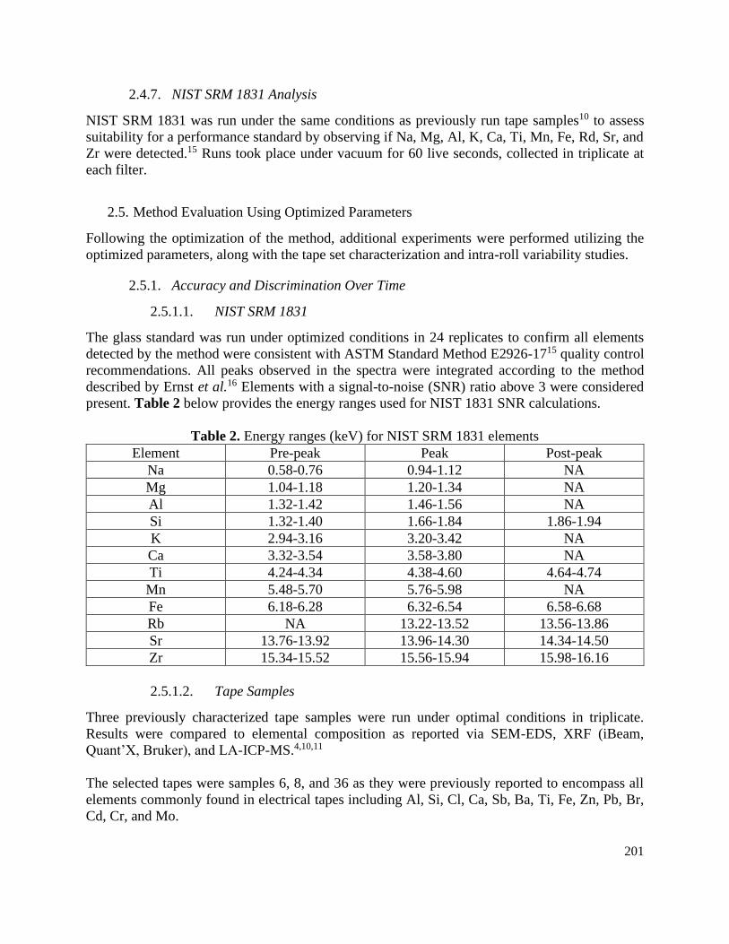
201
2.4.7. NIST SRM 1831 Analysis
NIST SRM 1831 was run under the same conditions as previously run tape samples10 to assess
suitability for a performance standard by observing if Na, Mg, Al, K, Ca, Ti, Mn, Fe, Rd, Sr, and
Zr were detected.15 Runs took place under vacuum for 60 live seconds, collected in triplicate at
each filter.
2.5. Method Evaluation Using Optimized Parameters
Following the optimization of the method, additional experiments were performed utilizing the
optimized parameters, along with the tape set characterization and intra-roll variability studies.
2.5.1. Accuracy and Discrimination Over Time
2.5.1.1. NIST SRM 1831
The glass standard was run under optimized conditions in 24 replicates to confirm all elements
detected by the method were consistent with ASTM Standard Method E2926-1715 quality control
recommendations. All peaks observed in the spectra were integrated according to the method
described by Ernst et al.16 Elements with a signal-to-noise (SNR) ratio above 3 were considered
present. Table 2 below provides the energy ranges used for NIST 1831 SNR calculations.
Table 2. Energy ranges (keV) for NIST SRM 1831 elements
Element Pre-peak Peak Post-peak
Na 0.58-0.76 0.94-1.12 NA
Mg 1.04-1.18 1.20-1.34 NA
Al 1.32-1.42 1.46-1.56 NA
Si 1.32-1.40 1.66-1.84 1.86-1.94
K 2.94-3.16 3.20-3.42 NA
Ca 3.32-3.54 3.58-3.80 NA
Ti 4.24-4.34 4.38-4.60 4.64-4.74
Mn 5.48-5.70 5.76-5.98 NA
Fe 6.18-6.28 6.32-6.54 6.58-6.68
Rb NA 13.22-13.52 13.56-13.86
Sr 13.76-13.92 13.96-14.30 14.34-14.50
Zr 15.34-15.52 15.56-15.94 15.98-16.16
2.5.1.2. Tape Samples
Three previously characterized tape samples were run under optimal conditions in triplicate.
Results were compared to elemental composition as reported via SEM-EDS, XRF (iBeam,
Quant’X, Bruker), and LA-ICP-MS.4,10,11
The selected tapes were samples 6, 8, and 36 as they were previously reported to encompass all
elements commonly found in electrical tapes including Al, Si, Cl, Ca, Sb, Ba, Ti, Fe, Zn, Pb, Br,
Cd, Cr, and Mo.
202
2.5.2. Sensitivity
2.5.2.1. NIST SRM 1831
NIST SRM 1831 was analyzed under optimal conditions in 24 replicates. Limits of detection
(LOD) were estimated for detected elements.
2.5.2.2. Tape Samples
The tape samples from Section 2.5.1.2. with the addition of tape sample 91 (a contemporary
formulation) were analyzed under optimal conditions in triplicate. Results from SEM-EDS, other
XRF instruments, and LA-ICP-MS were compared for each element to evaluate differences in
sensitivity between techniques.
2.5.3. Precision
2.5.3.1. Tape Samples
Tape sample 10, the same tape selected as the blind duplicate in the previous study,10 was run
under the same conditions both in the morning and afternoon for ten days over three weeks of the
study. The Cl/Ca ratio was selected for monitoring of repeatability and intermediate precision, as
this ratio had the greatest variation between samples. The assessment was performed through
spectral overlay and analysis of relative standard deviation values.
2.5.4. Selectivity
Tape samples determined to exhibit either Ca/Sb or Ba/Ti interferences during the previous study
were re-analyzed under optimal conditions to determine if any of these elements were resolved.
Selected samples are provided below:
a. Ba/Ti only: Sample 6
b. Ba/Ti and Ca/Sb: Sample 8
c. Ca/Sb only: Sample 36
2.6. Tape Set Characterization and Discrimination (N=94)
Each tape sample in the set of 94 was run in triplicate under optimal conditions. All peaks observed
in the spectra were integrated according to the method described by Ernst et al.16 Elements with a
signal-to-noise (SNR) ratio above 3 were used for comparisons. Table 3 below provides the energy
ranges used for tape element calculations. Examples of peak appearance for various SNR values
both below, near, and above the selected threshold of 3 are provided in Figures A.1-A.3 of the
Appendix.
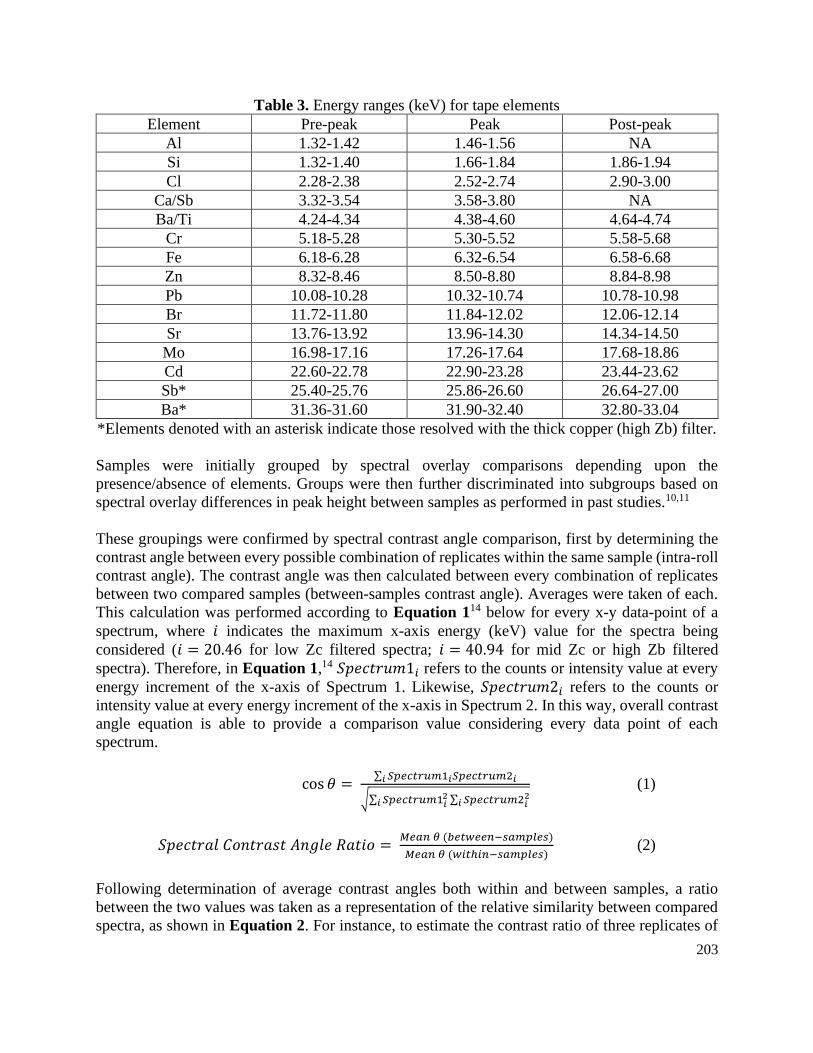
203
Table 3. Energy ranges (keV) for tape elements
Element Pre-peak Peak Post-peak
Al 1.32-1.42 1.46-1.56 NA
Si 1.32-1.40 1.66-1.84 1.86-1.94
Cl 2.28-2.38 2.52-2.74 2.90-3.00
Ca/Sb 3.32-3.54 3.58-3.80 NA
Ba/Ti 4.24-4.34 4.38-4.60 4.64-4.74
Cr 5.18-5.28 5.30-5.52 5.58-5.68
Fe 6.18-6.28 6.32-6.54 6.58-6.68
Zn 8.32-8.46 8.50-8.80 8.84-8.98
Pb 10.08-10.28 10.32-10.74 10.78-10.98
Br 11.72-11.80 11.84-12.02 12.06-12.14
Sr 13.76-13.92 13.96-14.30 14.34-14.50
Mo 16.98-17.16 17.26-17.64 17.68-18.86
Cd 22.60-22.78 22.90-23.28 23.44-23.62
Sb* 25.40-25.76 25.86-26.60 26.64-27.00
Ba* 31.36-31.60 31.90-32.40 32.80-33.04
*Elements denoted with an asterisk indicate those resolved with the thick copper (high Zb) filter.
Samples were initially grouped by spectral overlay comparisons depending upon the
presence/absence of elements. Groups were then further discriminated into subgroups based on
spectral overlay differences in peak height between samples as performed in past studies.10,11
These groupings were confirmed by spectral contrast angle comparison, first by determining the
contrast angle between every possible combination of replicates within the same sample (intra-roll
contrast angle). The contrast angle was then calculated between every combination of replicates
between two compared samples (between-samples contrast angle). Averages were taken of each.
This calculation was performed according to Equation 114 below for every x-y data-point of a
spectrum, where 𝑖 indicates the maximum x-axis energy (keV) value for the spectra being
considered (𝑖 = 20.46 for low Zc filtered spectra; 𝑖 = 40.94 for mid Zc or high Zb filtered
spectra). Therefore, in Equation 1,14 𝑆𝑝𝑒𝑐𝑡𝑟𝑢𝑚1𝑖 refers to the counts or intensity value at every
energy increment of the x-axis of Spectrum 1. Likewise, 𝑆𝑝𝑒𝑐𝑡𝑟𝑢𝑚2𝑖 refers to the counts or
intensity value at every energy increment of the x-axis in Spectrum 2. In this way, overall contrast
angle equation is able to provide a comparison value considering every data point of each
spectrum.
cos 𝜃 = ∑ 𝑆𝑝𝑒𝑐𝑡𝑟𝑢𝑚1𝑖𝑆𝑝𝑒𝑐𝑡𝑟𝑢𝑚2𝑖𝑖
√∑ 𝑆𝑝𝑒𝑐𝑡𝑟𝑢𝑚1𝑖2
𝑖 ∑ 𝑆𝑝𝑒𝑐𝑡𝑟𝑢𝑚2𝑖2
𝑖
(1)
𝑆𝑝𝑒𝑐𝑡𝑟𝑎𝑙 𝐶𝑜𝑛𝑡𝑟𝑎𝑠𝑡 𝐴𝑛𝑔𝑙𝑒 𝑅𝑎𝑡𝑖𝑜 = 𝑀𝑒𝑎𝑛 𝜃 (𝑏𝑒𝑡𝑤𝑒𝑒𝑛−𝑠𝑎𝑚𝑝𝑙𝑒𝑠)
𝑀𝑒𝑎𝑛 𝜃 (𝑤𝑖𝑡ℎ𝑖𝑛−𝑠𝑎𝑚𝑝𝑙𝑒𝑠) (2)
Following determination of average contrast angles both within and between samples, a ratio
between the two values was taken as a representation of the relative similarity between compared
spectra, as shown in Equation 2. For instance, to estimate the contrast ratio of three replicates of
204
sample A (A1, A2, A3) and three replicates of sample B (B1, B2, B3), the numerator will be
calculated from the mean contrast angle of all comparison pairs between the two spectra. That is,
the between-sample contrast angle will be the mean of the contrast angle of the following spectral
comparisons: A1-B1, A1-B2, A1-B3, A2-B1, A2-B2, A2-B3, A3-B1, A3-B2 and A3-B3. Then,
the denominator is calculated as the mean of all comparisons within the same sample (A1-A2, A1-
A3, A2-A3, and B1-B2, B1-B3 and B2-B3). A larger value indicates greater between-sample
difference relative to the intra-roll variation, while a smaller value indicates more similarities
between the compared samples.
The intra-sample contrast angle ratio was determined for all possible comparison pairs of samples
considered indistinguishable through spectral overlay from groups 4b, 5, 9a-d, 15, 17, 19a, 23, and
31a (see Table A.2 in the Appendix, n=132 comparison pairs) and from all possible comparison
pairs from the 20 fragments originating from the same roll (n=190 comparison pairs). The mean
and standard deviation of the ratio values were determined to establish an expected range of an
“indistinguishable sample” contrast ratio (e.g., same source, same group, same roll). Inter-sample
contrast angle ratios were then determined between samples considered distinguished by spectral
overlay, one from each subgroup (e.g., different source samples n=21 comparisons) and all
possible comparison pairs between samples of different groups (n=794 comparisons). The intra-
sample ratio was then used as a threshold to estimate similarity between spectra. If the mean
contrast angle for the samples compared fell outside the range of intra-samples, the samples were
considered different by XRF. All calculations were conducted in Microsoft Excel (Version 19.08)
and R Studio (Version 3.6.1) and a copy of the calculation templates is provided in the
Supplementary Material.
Quadratic Discriminant Analysis (QDA) was also performed on the overall dataset to observe
clustering due to elemental similarities or differences between varying tape countries of
manufacture. QDA was performed in JMP® Pro Software Version 14.0.0. It should be noted that
all spectral comparisons, both overlays and statistical analyses, were performed on spectra with
normalized counts.
2.7. Intra-roll Variability Study
In a similar manner to the previous study, an additional tape roll (Super 33+, Scotch 3M®, Saint
Paul, MN) was selected to analyze intra-source variability with newly optimized parameters.
Twenty samples were taken from the roll, with the first sample being 38” from the starting edge
of the roll and the remaining 19 taken every 38” into the roll. These increments were selected to
account for evenly spaced samplings across the entire length of the roll. All samples were analyzed
in triplicate under optimal conditions. Data analysis consisted of spectral overlay and spectral
contrast angle ratio comparisons between intra-roll samples, per filtering condition, to determine
any exclusionary differences.
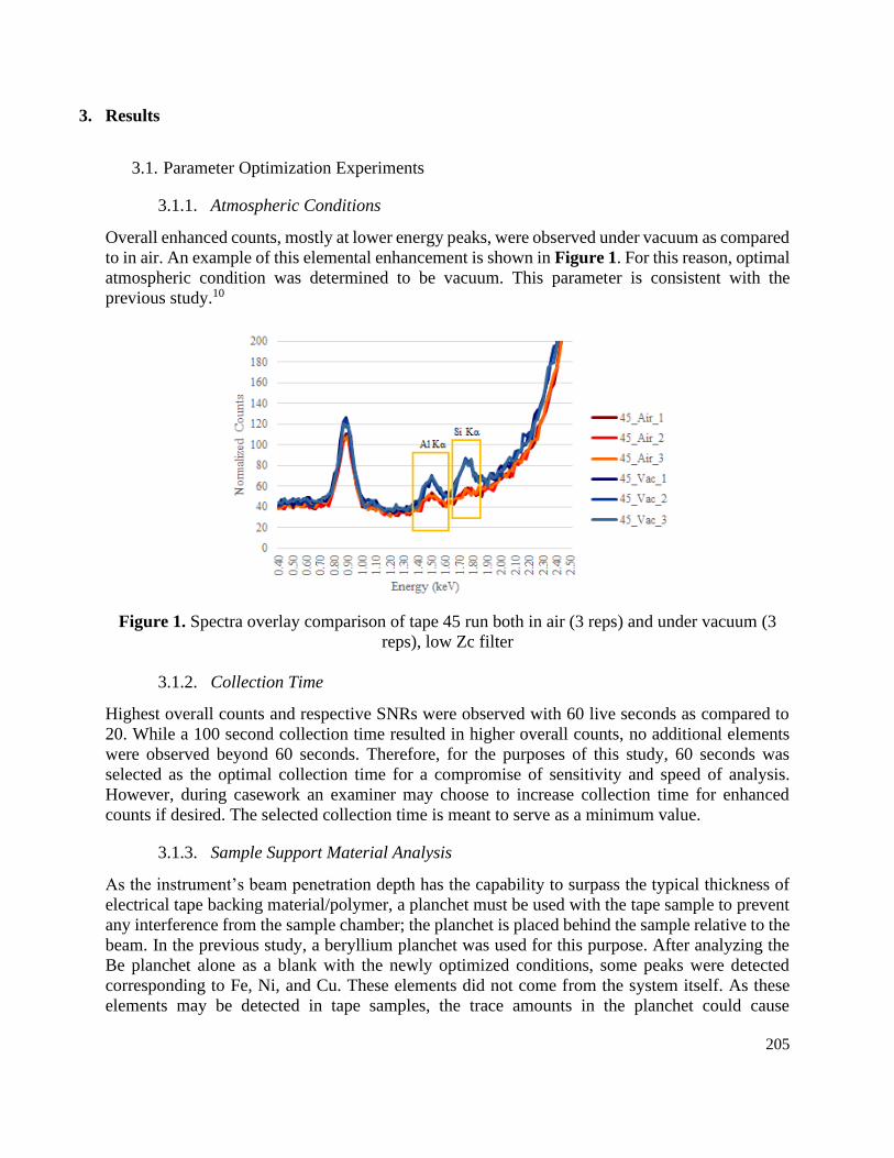
205
3. Results
3.1. Parameter Optimization Experiments
3.1.1. Atmospheric Conditions
Overall enhanced counts, mostly at lower energy peaks, were observed under vacuum as compared
to in air. An example of this elemental enhancement is shown in Figure 1. For this reason, optimal
atmospheric condition was determined to be vacuum. This parameter is consistent with the
previous study.10
Figure 1. Spectra overlay comparison of tape 45 run both in air (3 reps) and under vacuum (3
reps), low Zc filter
3.1.2. Collection Time
Highest overall counts and respective SNRs were observed with 60 live seconds as compared to
20. While a 100 second collection time resulted in higher overall counts, no additional elements
were observed beyond 60 seconds. Therefore, for the purposes of this study, 60 seconds was
selected as the optimal collection time for a compromise of sensitivity and speed of analysis.
However, during casework an examiner may choose to increase collection time for enhanced
counts if desired. The selected collection time is meant to serve as a minimum value.
3.1.3. Sample Support Material Analysis
As the instrument’s beam penetration depth has the capability to surpass the typical thickness of
electrical tape backing material/polymer, a planchet must be used with the tape sample to prevent
any interference from the sample chamber; the planchet is placed behind the sample relative to the
beam. In the previous study, a beryllium planchet was used for this purpose. After analyzing the
Be planchet alone as a blank with the newly optimized conditions, some peaks were detected
corresponding to Fe, Ni, and Cu. These elements did not come from the system itself. As these
elements may be detected in tape samples, the trace amounts in the planchet could cause
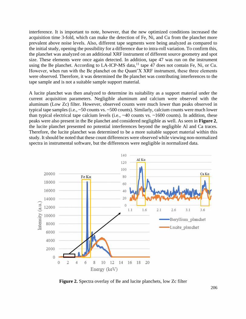
206
interference. It is important to note, however, that the new optimized conditions increased the
acquisition time 3-fold, which can make the detection of Fe, Ni, and Cu from the planchet more
prevalent above noise levels. Also, different tape segments were being analyzed as compared to
the initial study, opening the possibility for a difference due to intra-roll variation. To confirm this,
the planchet was analyzed on an additional XRF instrument of different source geometry and spot
size. These elements were once again detected. In addition, tape 47 was run on the instrument
using the Be planchet. According to LA-ICP-MS data,11 tape 47 does not contain Fe, Ni, or Cu.
However, when run with the Be planchet on the Quant’X XRF instrument, these three elements
were observed. Therefore, it was determined the Be planchet was contributing interferences to the
tape sample and is not a suitable sample support material.
A lucite planchet was then analyzed to determine its suitability as a support material under the
current acquisition parameters. Negligible aluminum and calcium were observed with the
aluminum (Low Zc) filter. However, observed counts were much lower than peaks observed in
typical tape samples (i.e., ~50 counts vs. ~500 counts). Similarly, calcium counts were much lower
than typical electrical tape calcium levels (i.e., ~40 counts vs. ~1600 counts). In addition, these
peaks were also present in the Be planchet and considered negligible as well. As seen in Figure 2,
the lucite planchet presented no potential interferences beyond the negligible Al and Ca traces.
Therefore, the lucite planchet was determined to be a more suitable support material within this
study. It should be noted that these count differences were observed while viewing non-normalized
spectra in instrumental software, but the differences were negligible in normalized data.
Figure 2. Spectra overlay of Be and lucite planchets, low Zc filter
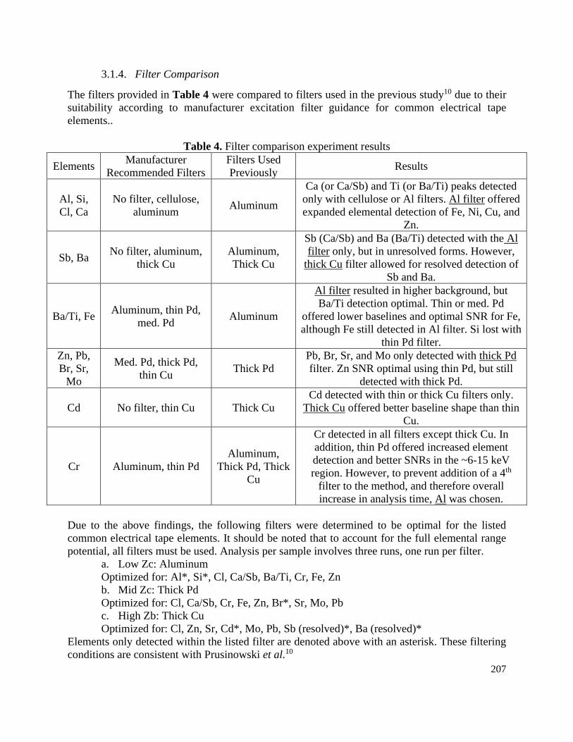
207
3.1.4. Filter Comparison
The filters provided in Table 4 were compared to filters used in the previous study10 due to their
suitability according to manufacturer excitation filter guidance for common electrical tape
elements..
Table 4. Filter comparison experiment results
Elements Manufacturer
Recommended Filters
Filters Used
Previously Results
Al, Si,
Cl, Ca
No filter, cellulose,
aluminum Aluminum
Ca (or Ca/Sb) and Ti (or Ba/Ti) peaks detected
only with cellulose or Al filters. Al filter offered
expanded elemental detection of Fe, Ni, Cu, and
Zn.
Sb, Ba No filter, aluminum,
thick Cu
Aluminum,
Thick Cu
Sb (Ca/Sb) and Ba (Ba/Ti) detected with the Al
filter only, but in unresolved forms. However,
thick Cu filter allowed for resolved detection of
Sb and Ba.
Ba/Ti, Fe Aluminum, thin Pd,
med. Pd Aluminum
Al filter resulted in higher background, but
Ba/Ti detection optimal. Thin or med. Pd
offered lower baselines and optimal SNR for Fe,
although Fe still detected in Al filter. Si lost with
thin Pd filter.
Zn, Pb,
Br, Sr,
Mo
Med. Pd, thick Pd,
thin Cu Thick Pd
Pb, Br, Sr, and Mo only detected with thick Pd
filter. Zn SNR optimal using thin Pd, but still
detected with thick Pd.
Cd No filter, thin Cu Thick Cu
Cd detected with thin or thick Cu filters only.
Thick Cu offered better baseline shape than thin
Cu.
Cr Aluminum, thin Pd
Aluminum,
Thick Pd, Thick
Cu
Cr detected in all filters except thick Cu. In
addition, thin Pd offered increased element
detection and better SNRs in the ~6-15 keV
region. However, to prevent addition of a 4th
filter to the method, and therefore overall
increase in analysis time, Al was chosen.
Due to the above findings, the following filters were determined to be optimal for the listed
common electrical tape elements. It should be noted that to account for the full elemental range
potential, all filters must be used. Analysis per sample involves three runs, one run per filter.
a. Low Zc: Aluminum
Optimized for: Al*, Si*, Cl, Ca/Sb, Ba/Ti, Cr, Fe, Zn
b. Mid Zc: Thick Pd
Optimized for: Cl, Ca/Sb, Cr, Fe, Zn, Br*, Sr, Mo, Pb
c. High Zb: Thick Cu
Optimized for: Cl, Zn, Sr, Cd*, Mo, Pb, Sb (resolved)*, Ba (resolved)*
Elements only detected within the listed filter are denoted above with an asterisk. These filtering
conditions are consistent with Prusinowski et al.10
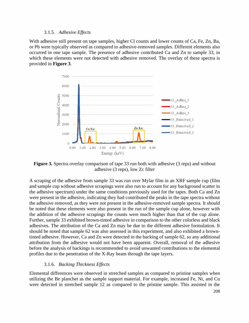
208
3.1.5. Adhesive Effects
With adhesive still present on tape samples, higher Cl counts and lower counts of Ca, Fe, Zn, Ba,
or Pb were typically observed as compared to adhesive-removed samples. Different elements also
occurred in one tape sample. The presence of adhesive contributed Ca and Zn to sample 33, in
which these elements were not detected with adhesive removed. The overlay of these spectra is
provided in Figure 3.
Figure 3. Spectra overlay comparison of tape 33 run both with adhesive (3 reps) and without
adhesive (3 reps), low Zc filter
A scraping of the adhesive from sample 33 was run over Mylar film in an XRF sample cup (film
and sample cup without adhesive scrapings were also run to account for any background scatter in
the adhesive spectrum) under the same conditions previously used for the tapes. Both Ca and Zn
were present in the adhesive, indicating they had contributed the peaks in the tape spectra without
the adhesive removed, as they were not present in the adhesive-removed sample spectra. It should
be noted that these elements were also present in the run of the sample cup alone, however with
the addition of the adhesive scrapings the counts were much higher than that of the cup alone.
Further, sample 33 exhibited brown-tinted adhesive in comparison to the other colorless and black
adhesives. The attribution of the Ca and Zn may be due to the different adhesive formulation. It
should be noted that sample 62 was also assessed in this experiment, and also exhibited a brown-
tinted adhesive. However, Ca and Zn were detected in the backing of sample 62, so any additional
attribution from the adhesive would not have been apparent. Overall, removal of the adhesive
before the analysis of backings is recommended to avoid unwanted contributions to the elemental
profiles due to the penetration of the X-Ray beam through the tape layers.
3.1.6. Backing Thickness Effects
Elemental differences were observed in stretched samples as compared to pristine samples when
utilizing the Be planchet as the sample support material. For example, increased Fe, Ni, and Cu
were detected in stretched sample 12 as compared to the pristine sample. This assisted in the
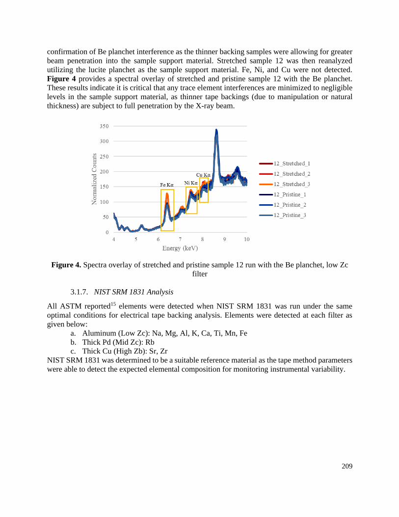
209
confirmation of Be planchet interference as the thinner backing samples were allowing for greater
beam penetration into the sample support material. Stretched sample 12 was then reanalyzed
utilizing the lucite planchet as the sample support material. Fe, Ni, and Cu were not detected.
Figure 4 provides a spectral overlay of stretched and pristine sample 12 with the Be planchet.
These results indicate it is critical that any trace element interferences are minimized to negligible
levels in the sample support material, as thinner tape backings (due to manipulation or natural
thickness) are subject to full penetration by the X-ray beam.
Figure 4. Spectra overlay of stretched and pristine sample 12 run with the Be planchet, low Zc
filter
3.1.7. NIST SRM 1831 Analysis
All ASTM reported15 elements were detected when NIST SRM 1831 was run under the same
optimal conditions for electrical tape backing analysis. Elements were detected at each filter as
given below:
a. Aluminum (Low Zc): Na, Mg, Al, K, Ca, Ti, Mn, Fe
b. Thick Pd (Mid Zc): Rb
c. Thick Cu (High Zb): Sr, Zr
NIST SRM 1831 was determined to be a suitable reference material as the tape method parameters
were able to detect the expected elemental composition for monitoring instrumental variability.
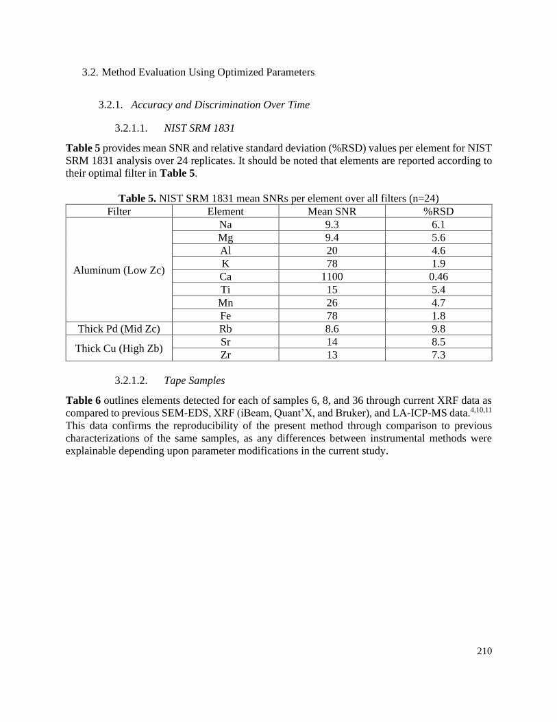
210
3.2. Method Evaluation Using Optimized Parameters
3.2.1. Accuracy and Discrimination Over Time
3.2.1.1. NIST SRM 1831
Table 5 provides mean SNR and relative standard deviation (%RSD) values per element for NIST
SRM 1831 analysis over 24 replicates. It should be noted that elements are reported according to
their optimal filter in Table 5.
Table 5. NIST SRM 1831 mean SNRs per element over all filters (n=24)
Filter Element Mean SNR %RSD
Aluminum (Low Zc)
Na 9.3 6.1
Mg 9.4 5.6
Al 20 4.6
K 78 1.9
Ca 1100 0.46
Ti 15 5.4
Mn 26 4.7
Fe 78 1.8
Thick Pd (Mid Zc) Rb 8.6 9.8
Thick Cu (High Zb) Sr 14 8.5
Zr 13 7.3
3.2.1.2. Tape Samples
Table 6 outlines elements detected for each of samples 6, 8, and 36 through current XRF data as
compared to previous SEM-EDS, XRF (iBeam, Quant’X, and Bruker), and LA-ICP-MS data.4,10,11
This data confirms the reproducibility of the present method through comparison to previous
characterizations of the same samples, as any differences between instrumental methods were
explainable depending upon parameter modifications in the current study.
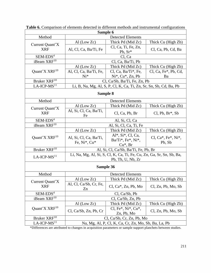
211
Table 6. Comparison of elements detected in different methods and instrumental configurations
Sample 6
Method Detected Elements
Current Quant’X
XRF
Al (Low Zc) Thick Pd (Mid Zc) Thick Cu (High Zb)
Al, Cl, Ca, Ba/Ti, Fe Cl, Ca, Ti, Fe, Zn,
Pb, Sr* Cl, Ca, Pb, Cd, Ba
SEM-EDS4 Cl, Ca
iBeam XRF10 Cl, Ca, Ba/Ti, Pb
Quant’X XRF10
Al (Low Zc) Thick Pd (Mid Zc) Thick Cu (High Zb)
Al, Cl, Ca, Ba/Ti, Fe,
Ni*
Cl, Ca, Ba/Ti*, Fe,
Ni*, Cu*, Zn, Pb
Cl, Ca, Fe*, Pb, Cd,
Ba
Bruker XRF10 Cl, Ca/Sb, Ba/Ti, Fe, Zn, Pb
LA-ICP-MS11 Li, B, Na, Mg, Al, S, P, Cl, K, Ca, Ti, Zn, Sr, Sn, Sb, Cd, Ba, Pb
Sample 8
Method Detected Elements
Current Quant’X
XRF
Al (Low Zc) Thick Pd (Mid Zc) Thick Cu (High Zb)
Al, Si, Cl, Ca, Ba/Ti,
Fe Cl, Ca, Pb, Br Cl, Pb, Br*, Sb
SEM-EDS4 Al, Si, Cl, Ca
iBeam XRF10 Al, Si, Cl, Ca, Ti, Fe
Quant’X XRF10
Al (Low Zc) Thick Pd (Mid Zc) Thick Cu (High Zb)
Al, Si, Cl, Ca, Ba/Ti,
Fe, Ni*, Cu*
Al*, Si*, Cl, Ca,
Ba/Ti*, Fe*, Ni*,
Cu*, Br
Cl, Ca*, Fe*, Ni*,
Pb, Sb
Bruker XRF10 Al, Si, Cl, Ca/Sb, Ba/Ti, Fe, Pb, Br
LA-ICP-MS11 Li, Na, Mg, Al, Si, S, Cl, K, Ca, Ti, Fe, Cu, Zn, Ga, Sr, Sn, Sb, Ba,
Pb, Th, U, Nb, Zr
Sample 36
Method Detected Elements
Current Quant’X
XRF
Al (Low Zc) Thick Pd (Mid Zc) Thick Cu (High Zb)
Al, Cl, Ca/Sb, Cr, Fe,
Zn Cl, Ca*, Zn, Pb, Mo Cl, Zn, Pb, Mo, Sb
SEM-EDS4 Cl, Ca/Sb, Pb
iBeam XRF10 Cl, Ca/Sb, Zn, Pb
Quant’X XRF10
Al (Low Zc) Thick Pd (Mid Zc) Thick Cu (High Zb)
Cl, Ca/Sb, Zn, Pb, Cr Cl, Fe*, Ni*, Cu*,
Zn, Pb, Mo Cl, Zn, Pb, Mo, Sb
Bruker XRF10 Cl, Ca/Sb, Cr, Zn, Pb, Mo
LA-ICP-MS11 Na, Mg, Al, P, Cl, K, Ca, Cr, Zn, Mo, Sb, Ba, La, Pb *Differences are attributed to changes in acquisition parameters or sample support planchets between studies.
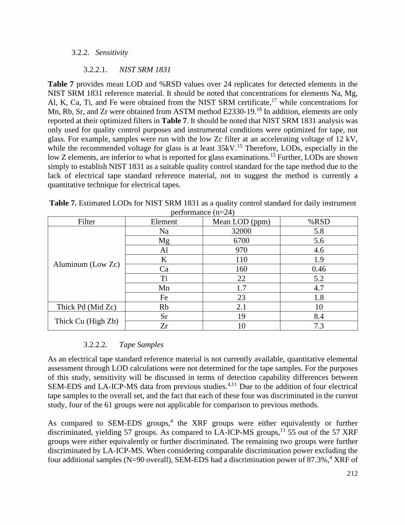
212
3.2.2. Sensitivity
3.2.2.1. NIST SRM 1831
Table 7 provides mean LOD and %RSD values over 24 replicates for detected elements in the
NIST SRM 1831 reference material. It should be noted that concentrations for elements Na, Mg,
Al, K, Ca, Ti, and Fe were obtained from the NIST SRM certificate,17 while concentrations for
Mn, Rb, Sr, and Zr were obtained from ASTM method E2330-19.18 In addition, elements are only
reported at their optimized filters in Table 7. It should be noted that NIST SRM 1831 analysis was
only used for quality control purposes and instrumental conditions were optimized for tape, not
glass. For example, samples were run with the low Zc filter at an accelerating voltage of 12 kV,
while the recommended voltage for glass is at least 35kV.15 Therefore, LODs, especially in the
low Z elements, are inferior to what is reported for glass examinations.15 Further, LODs are shown
simply to establish NIST 1831 as a suitable quality control standard for the tape method due to the
lack of electrical tape standard reference material, not to suggest the method is currently a
quantitative technique for electrical tapes.
Table 7. Estimated LODs for NIST SRM 1831 as a quality control standard for daily instrument
performance (n=24)
Filter Element Mean LOD (ppm) %RSD
Aluminum (Low Zc)
Na 32000 5.8
Mg 6700 5.6
Al 970 4.6
K 110 1.9
Ca 160 0.46
Ti 22 5.2
Mn 1.7 4.7
Fe 23 1.8
Thick Pd (Mid Zc) Rb 2.1 10
Thick Cu (High Zb) Sr 19 8.4
Zr 10 7.3
3.2.2.2. Tape Samples
As an electrical tape standard reference material is not currently available, quantitative elemental
assessment through LOD calculations were not determined for the tape samples. For the purposes
of this study, sensitivity will be discussed in terms of detection capability differences between
SEM-EDS and LA-ICP-MS data from previous studies.4,11 Due to the addition of four electrical
tape samples to the overall set, and the fact that each of these four was discriminated in the current
study, four of the 61 groups were not applicable for comparison to previous methods.
As compared to SEM-EDS groups,4 the XRF groups were either equivalently or further
discriminated, yielding 57 groups. As compared to LA-ICP-MS groups,11 55 out of the 57 XRF
groups were either equivalently or further discriminated. The remaining two groups were further
discriminated by LA-ICP-MS. When considering comparable discrimination power excluding the
four additional samples (N=90 overall), SEM-EDS had a discrimination power of 87.3%,4 XRF of
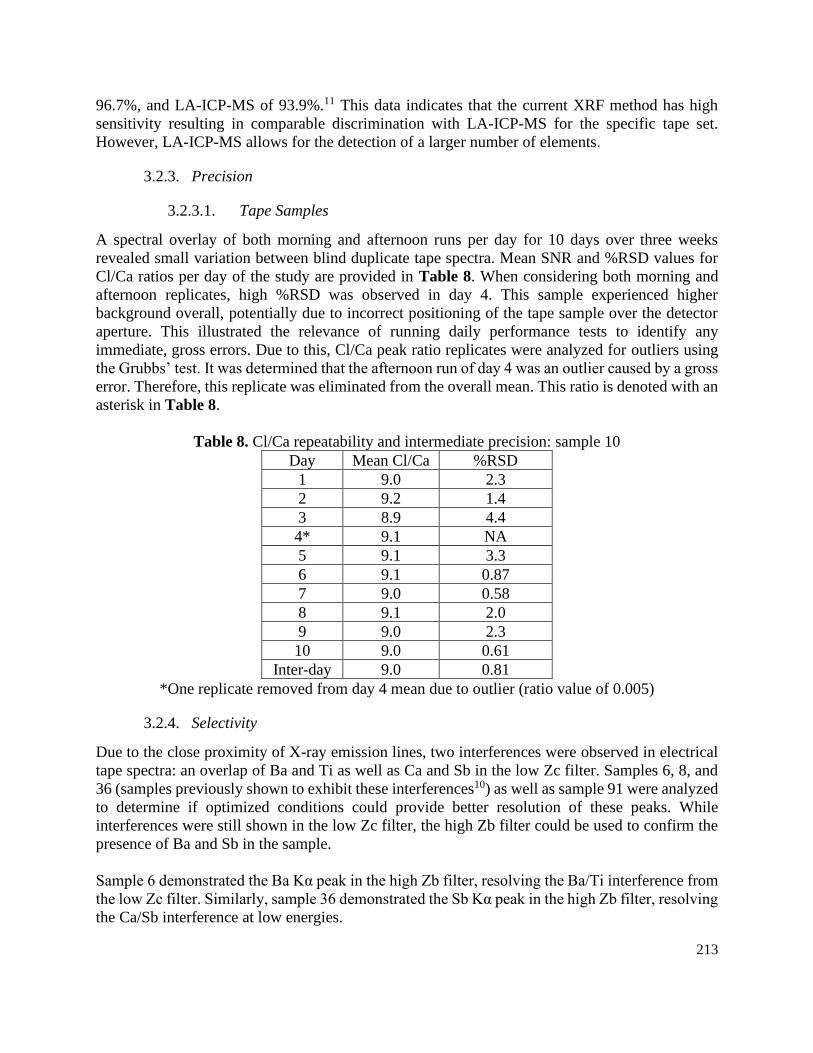
213
96.7%, and LA-ICP-MS of 93.9%.11 This data indicates that the current XRF method has high
sensitivity resulting in comparable discrimination with LA-ICP-MS for the specific tape set.
However, LA-ICP-MS allows for the detection of a larger number of elements.
3.2.3. Precision
3.2.3.1. Tape Samples
A spectral overlay of both morning and afternoon runs per day for 10 days over three weeks
revealed small variation between blind duplicate tape spectra. Mean SNR and %RSD values for
Cl/Ca ratios per day of the study are provided in Table 8. When considering both morning and
afternoon replicates, high %RSD was observed in day 4. This sample experienced higher
background overall, potentially due to incorrect positioning of the tape sample over the detector
aperture. This illustrated the relevance of running daily performance tests to identify any
immediate, gross errors. Due to this, Cl/Ca peak ratio replicates were analyzed for outliers using
the Grubbs’ test. It was determined that the afternoon run of day 4 was an outlier caused by a gross
error. Therefore, this replicate was eliminated from the overall mean. This ratio is denoted with an
asterisk in Table 8.
Table 8. Cl/Ca repeatability and intermediate precision: sample 10
Day Mean Cl/Ca %RSD
1 9.0 2.3
2 9.2 1.4
3 8.9 4.4
4* 9.1 NA
5 9.1 3.3
6 9.1 0.87
7 9.0 0.58
8 9.1 2.0
9 9.0 2.3
10 9.0 0.61
Inter-day 9.0 0.81
*One replicate removed from day 4 mean due to outlier (ratio value of 0.005)
3.2.4. Selectivity
Due to the close proximity of X-ray emission lines, two interferences were observed in electrical
tape spectra: an overlap of Ba and Ti as well as Ca and Sb in the low Zc filter. Samples 6, 8, and
36 (samples previously shown to exhibit these interferences10) as well as sample 91 were analyzed
to determine if optimized conditions could provide better resolution of these peaks. While
interferences were still shown in the low Zc filter, the high Zb filter could be used to confirm the
presence of Ba and Sb in the sample.
Sample 6 demonstrated the Ba Kα peak in the high Zb filter, resolving the Ba/Ti interference from
the low Zc filter. Similarly, sample 36 demonstrated the Sb Kα peak in the high Zb filter, resolving
the Ca/Sb interference at low energies.
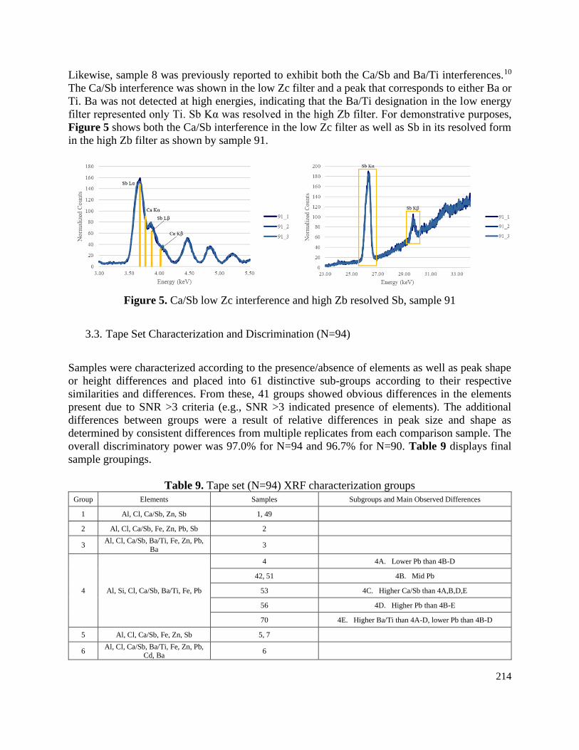
214
Likewise, sample 8 was previously reported to exhibit both the Ca/Sb and Ba/Ti interferences.10
The Ca/Sb interference was shown in the low Zc filter and a peak that corresponds to either Ba or
Ti. Ba was not detected at high energies, indicating that the Ba/Ti designation in the low energy
filter represented only Ti. Sb Kα was resolved in the high Zb filter. For demonstrative purposes,
Figure 5 shows both the Ca/Sb interference in the low Zc filter as well as Sb in its resolved form
in the high Zb filter as shown by sample 91.
Figure 5. Ca/Sb low Zc interference and high Zb resolved Sb, sample 91
3.3. Tape Set Characterization and Discrimination (N=94)
Samples were characterized according to the presence/absence of elements as well as peak shape
or height differences and placed into 61 distinctive sub-groups according to their respective
similarities and differences. From these, 41 groups showed obvious differences in the elements
present due to SNR >3 criteria (e.g., SNR >3 indicated presence of elements). The additional
differences between groups were a result of relative differences in peak size and shape as
determined by consistent differences from multiple replicates from each comparison sample. The
overall discriminatory power was 97.0% for N=94 and 96.7% for N=90. Table 9 displays final
sample groupings.
Table 9. Tape set (N=94) XRF characterization groups Group Elements Samples Subgroups and Main Observed Differences
1 Al, Cl, Ca/Sb, Zn, Sb 1, 49
2 Al, Cl, Ca/Sb, Fe, Zn, Pb, Sb 2
3 Al, Cl, Ca/Sb, Ba/Ti, Fe, Zn, Pb,
Ba 3
4 Al, Si, Cl, Ca/Sb, Ba/Ti, Fe, Pb
4 4A. Lower Pb than 4B-D
42, 51 4B. Mid Pb
53 4C. Higher Ca/Sb than 4A,B,D,E
56 4D. Higher Pb than 4B-E
70 4E. Higher Ba/Ti than 4A-D, lower Pb than 4B-D
5 Al, Cl, Ca/Sb, Fe, Zn, Sb 5, 7
6 Al, Cl, Ca/Sb, Ba/Ti, Fe, Zn, Pb,
Cd, Ba 6
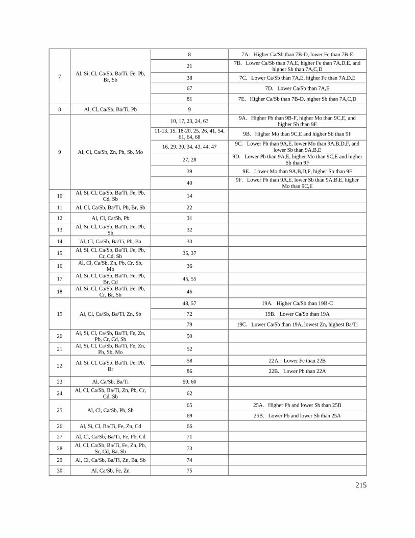
215
7 Al, Si, Cl, Ca/Sb, Ba/Ti, Fe, Pb,
Br, Sb
8 7A. Higher Ca/Sb than 7B-D, lower Fe than 7B-E
21 7B. Lower Ca/Sb than 7A,E, higher Fe than 7A,D,E, and
higher Sb than 7A,C,D
38 7C. Lower Ca/Sb than 7A,E, higher Fe than 7A,D,E
67 7D. Lower Ca/Sb than 7A,E
81 7E. Higher Ca/Sb than 7B-D, higher Sb than 7A,C,D
8 Al, Cl, Ca/Sb, Ba/Ti, Pb 9
9 Al, Cl, Ca/Sb, Zn, Pb, Sb, Mo
10, 17, 23, 24, 63 9A. Higher Pb than 9B-F, higher Mo than 9C,E, and
higher Sb than 9F
11-13, 15, 18-20, 25, 26, 41, 54, 61, 64, 68
9B. Higher Mo than 9C,E and higher Sb than 9F
16, 29, 30, 34, 43, 44, 47 9C. Lower Pb than 9A,E, lower Mo than 9A,B,D,F, and
lower Sb than 9A,B,E
27, 28 9D. Lower Pb than 9A,E, higher Mo than 9C,E and higher
Sb than 9F
39 9E. Lower Mo than 9A,B,D,F, higher Sb than 9F
40 9F. Lower Pb than 9A,E, lower Sb than 9A,B,E, higher
Mo than 9C,E
10 Al, Si, Cl, Ca/Sb, Ba/Ti, Fe, Pb,
Cd, Sb 14
11 Al, Cl, Ca/Sb, Ba/Ti, Pb, Br, Sb 22
12 Al, Cl, Ca/Sb, Pb 31
13 Al, Si, Cl, Ca/Sb, Ba/Ti, Fe, Pb,
Sb 32
14 Al, Cl, Ca/Sb, Ba/Ti, Pb, Ba 33
15 Al, Si, Cl, Ca/Sb, Ba/Ti, Fe, Pb,
Cr, Cd, Sb 35, 37
16 Al, Cl, Ca/Sb, Zn, Pb, Cr, Sb,
Mo 36
17 Al, Si, Cl, Ca/Sb, Ba/Ti, Fe, Pb,
Br, Cd 45, 55
18 Al, Si, Cl, Ca/Sb, Ba/Ti, Fe, Pb,
Cr, Br, Sb 46
19 Al, Cl, Ca/Sb, Ba/Ti, Zn, Sb
48, 57 19A. Higher Ca/Sb than 19B-C
72 19B. Lower Ca/Sb than 19A
79 19C. Lower Ca/Sb than 19A, lowest Zn, highest Ba/Ti
20 Al, Si, Cl, Ca/Sb, Ba/Ti, Fe, Zn,
Pb, Cr, Cd, Sb 50
21 Al, Si, Cl, Ca/Sb, Ba/Ti, Fe, Zn,
Pb, Sb, Mo 52
22 Al, Si, Cl, Ca/Sb, Ba/Ti, Fe, Pb,
Br
58 22A. Lower Fe than 22B
86 22B. Lower Pb than 22A
23 Al, Ca/Sb, Ba/Ti 59, 60
24 Al, Cl, Ca/Sb, Ba/Ti, Zn, Pb, Cr,
Cd, Sb 62
25 Al, Cl, Ca/Sb, Pb, Sb 65 25A. Higher Pb and lower Sb than 25B
69 25B. Lower Pb and lower Sb than 25A
26 Al, Si, Cl, Ba/Ti, Fe, Zn, Cd 66
27 Al, Cl, Ca/Sb, Ba/Ti, Fe, Pb, Cd 71
28 Al, Cl, Ca/Sb, Ba/Ti, Fe, Zn, Pb,
Sr, Cd, Ba, Sb 73
29 Al, Cl, Ca/Sb, Ba/Ti, Zn, Ba, Sb 74
30 Al, Ca/Sb, Fe, Zn 75
216
31 Al, Cl, Ca/Sb, Ba/Ti, Zn, Ba, Sb,
Mo
76, 77, 83 31A. Lower Sb than 31B
80 31B. Higher Sb than 31A
78 31C. Lowest Ca/Sb, Mo, and Sb, highest Cl
91 31D. Lower Sb than 31A-B
32 Al, Si, Cl, Ca/Sb, Ba/Ti, Fe, Zn,
Pb, Br 82
33 Al, Cl, Ca/Sb, Ba/Ti, Zn, Br, Sb 84
34 Al, Cl, Ca/Sb, Ba/Ti, Fe, Zn, Pb,
Cr, Cd, Sb 85
35 Al, Cl, Ca/Sb, Ba/Ti, Zn 87
36 Al, Cl, Ca/Sb, Ba/Ti, Fe, Zn 88
37 Al, Cl, Ca/Sb, Ba/Ti, Zn, Pb, Cd,
Sb 89
38 Al, Cl, Ca/Sb, Ba/Ti, Fe, Pb, Cd,
Sb 90
39 Al, Cl, Ca/Sb, Ba/Ti, Zn, Pb, Ba,
Sb, Mo 92
40 Al, Cl, Ca/Sb, Ba/Ti, Fe, Zn, Sr,
Br, Ba, Sb 93
41 Al, Cl, Ca/Sb, Ba/Ti, Fe, Zn, Sb 94
3.3.1. Spectral Contrast Angle Comparison
Spectral overlay is a recognized method for the comparison of EDS spectra (e.g., SEM-EDS and
XRF)3,4,10 and is widely implemented in forensic laboratories as the first step for identifying
spectral differences or similarities. Replicates of the known and questioned spectra are overlaid to
assess variability of each sample. When variability of spectral shape and intensity of the questioned
sample is greater than the intra-roll variability of the known sample, then the samples are
distinguished by EDS or XRF. Large differences between samples are easy to detect by this
method. However, comparing spectra by visual methods, such as spectral overlay, becomes more
challenging with increased similarity between spectra. As a result, the judgment of similarity of
spectra becomes more complex and adds subjectivity. This is a common problem not only in
forensic science but in spectrochemical comparisons in general.
To deal with these situations, analytical scientists have reported alternative methods for the
comparison of spectra.14,19,20 In this study, we exhibit a complementary method for the
confirmation of spectra overlay by applying well known, vector-based spectral comparison using
contrast angles. This method is widely applied in spectral library searching (e.g., FTIR, mass
spectra).14,19 However, unlike spectral overlay, the contrast angle ratio is not yet applied for routine
tape comparisons. This study aims to evaluate the utility of spectral contrast angle as a potential
complementary tool that could be used in the future to support examiner opinion.
In order to confirm sub-groups made by observed spectral differences (spectra overlay), the
spectral contrast angle was found in every combination both within sample replicates and between
sample replicates. These values were used to create a ratio of between-sample mean contrast angle
to intra-roll mean contrast angle. Ratios were determined between all combinations of sample pairs
considered indistinguishable through spectral overlay and through samples from the same roll.
Ratios were also determined between those samples determined to be distinguishable, and thus
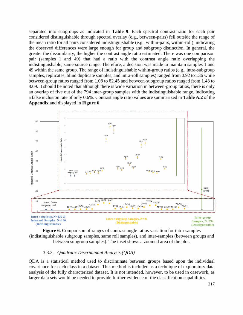
217
separated into subgroups as indicated in Table 9. Each spectral contrast ratio for each pair
considered distinguishable through spectral overlay (e.g., between-pairs) fell outside the range of
the mean ratio for all pairs considered indistinguishable (e.g., within-pairs, within-roll), indicating
the observed differences were large enough for group and subgroup distinction. In general, the
greater the dissimilarity, the higher the contrast angle ratio estimated. There was one comparison
pair (samples 1 and 49) that had a ratio with the contrast angle ratio overlapping the
indistinguishable, same-source range. Therefore, a decision was made to maintain samples 1 and
49 within the same group. The range of indistinguishable within-group ratios (e.g., intra-subgroup
samples, replicates, blind duplicate samples, and intra-roll samples) ranged from 0.92 to1.36 while
between-group ratios ranged from 1.08 to 82.45 and between-subgroup ratios ranged from 1.43 to
8.09. It should be noted that although there is wide variation in between-group ratios, there is only
an overlap of five out of the 794 inter-group samples with the indistinguishable range, indicating
a false inclusion rate of only 0.6%. Contrast angle ratio values are summarized in Table A.2 of the
Appendix and displayed in Figure 6.
Figure 6. Comparison of ranges of contrast angle ratios variation for intra-samples
(indistinguishable subgroup samples, same roll samples), and inter-samples (between groups and
between subgroup samples). The inset shows a zoomed area of the plot.
3.3.2. Quadratic Discriminant Analysis (QDA)
QDA is a statistical method used to discriminate between groups based upon the individual
covariance for each class in a dataset. This method is included as a technique of exploratory data
analysis of the fully characterized dataset. It is not intended, however, to be used in casework, as
larger data sets would be needed to provide further evidence of the classification capabilities.
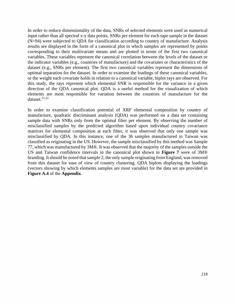
218
In order to reduce dimensionality of the data, SNRs of selected elements were used as numerical
input rather than all spectral x-y data points. SNRs per element for each tape sample in the dataset
(N=94) were subjected to QDA for classification according to country of manufacture. Analysis
results are displayed in the form of a canonical plot in which samples are represented by points
corresponding to their multivariate means and are plotted in terms of the first two canonical
variables. These variables represent the canonical correlation between the levels of the dataset or
the indicator variables (e.g., countries of manufacture) and the covariates or characteristics of the
dataset (e.g., SNRs per element). The first two canonical variables represent the dimensions of
optimal separation for the dataset. In order to examine the loadings of these canonical variables,
or the weight each covariate holds in relation to a canonical variable, biplot rays are observed. For
this study, the rays represent which elemental SNR is responsible for the variance in a given
direction of the QDA canonical plot. QDA is a useful method for the visualization of which
elements are most responsible for variation between the countries of manufacture for the
dataset.21,22
In order to examine classification potential of XRF elemental composition by country of
manufacture, quadratic discriminant analysis (QDA) was performed on a data set containing
sample data with SNRs only from the optimal filter per element. By observing the number of
misclassified samples by the predicted algorithm based upon individual country covariance
matrices for elemental composition at each filter, it was observed that only one sample was
misclassified by QDA. In this instance, one of the 36 samples manufactured in Taiwan was
classified as originating in the US. However, the sample misclassified by this method was Sample
77, which was manufactured by 3M®. It was observed that the majority of the samples outside the
US and Taiwan confidence intervals in the canonical plot shown in Figure 7 were of 3M®
branding. It should be noted that sample 2, the only sample originating from England, was removed
from this dataset for ease of view of country clustering. QDA biplots displaying the loadings
(vectors showing by which elements samples are most variable) for the data set are provided in
Figure A.4 of the Appendix.
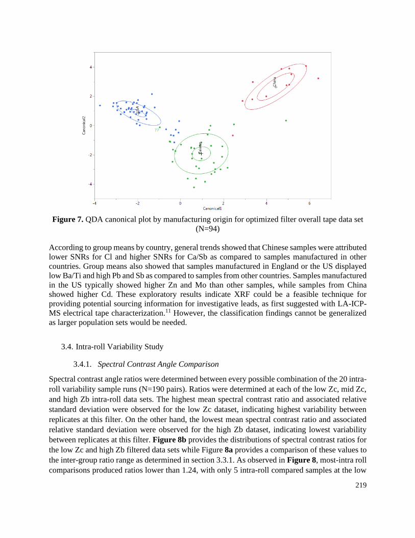
219
Figure 7. QDA canonical plot by manufacturing origin for optimized filter overall tape data set
(N=94)
According to group means by country, general trends showed that Chinese samples were attributed
lower SNRs for Cl and higher SNRs for Ca/Sb as compared to samples manufactured in other
countries. Group means also showed that samples manufactured in England or the US displayed
low Ba/Ti and high Pb and Sb as compared to samples from other countries. Samples manufactured
in the US typically showed higher Zn and Mo than other samples, while samples from China
showed higher Cd. These exploratory results indicate XRF could be a feasible technique for
providing potential sourcing information for investigative leads, as first suggested with LA-ICP-
MS electrical tape characterization.11 However, the classification findings cannot be generalized
as larger population sets would be needed.
3.4. Intra-roll Variability Study
3.4.1. Spectral Contrast Angle Comparison
Spectral contrast angle ratios were determined between every possible combination of the 20 intra-
roll variability sample runs (N=190 pairs). Ratios were determined at each of the low Zc, mid Zc,
and high Zb intra-roll data sets. The highest mean spectral contrast ratio and associated relative
standard deviation were observed for the low Zc dataset, indicating highest variability between
replicates at this filter. On the other hand, the lowest mean spectral contrast ratio and associated
relative standard deviation were observed for the high Zb dataset, indicating lowest variability
between replicates at this filter. Figure 8b provides the distributions of spectral contrast ratios for
the low Zc and high Zb filtered data sets while Figure 8a provides a comparison of these values to
the inter-group ratio range as determined in section 3.3.1. As observed in Figure 8, most-intra roll
comparisons produced ratios lower than 1.24, with only 5 intra-roll compared samples at the low
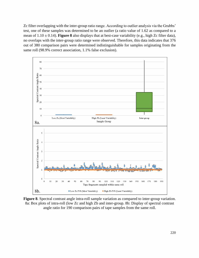
220
Zc filter overlapping with the inter-group ratio range. According to outlier analysis via the Grubbs’
test, one of these samples was determined to be an outlier (a ratio value of 1.62 as compared to a
mean of 1.10 ± 0.14). Figure 8 also displays that at best-case variability (e.g., high Zc filter data),
no overlaps with the inter-group ratio range were observed. Therefore, this data indicates that 376
out of 380 comparison pairs were determined indistinguishable for samples originating from the
same roll (98.9% correct association, 1.1% false exclusion).
Figure 8. Spectral contrast angle intra-roll sample variation as compared to inter-group variation.
8a: Box plots of intra-roll (low Zc and high Zb and inter-group. 8b: Display of spectral contrast
angle ratio for 190 comparison pairs of tape samples from the same roll.
221
4. Conclusions
XRF is a rapid, sensitive addition for highly discriminatory electrical tape backing analysis. The
discrimination achieved through XRF analysis alone, as demonstrated in this study, is comparable
to discrimination achieved both through a full analytical scheme (physical observations and
measurements, FTIR, py-GC/MS, and SEM-EDS) for electrical tape backings and LA-ICP-MS
characterization (i.e., for N=90, 96.7% as compared to 94.3% and 93.9%, respectively).4,11 This
technique is well suited for quick screening with accuracy and discrimination over time, precision,
sensitivity, and selectivity.
This study also highlighted the high inter-sample variability and low intra-sample variability of
electrical tape backings as characterized through the optimized XRF method. While these metrics
were only measured on a set of 94 tapes, this set represents a variety of tapes from various brands
and four different countries of manufacture including the US, China, Taiwan, and England.
Therefore, this data provides insight into the expected variation both between electrical tape types
as well as within a single roll.
It is critical for forensic examiners to have access to rapid, highly discriminatory techniques for
optimal utilization of the probative value of submitted evidence items. This method provides an
additional tool to traditional electrical tape chemical analysis. The optimization process described
through this study suggests proper parameters for XRF electrical tape analysis, and the additional
experiments using those optimized parameters provides a model of the key factors and potential
interferences to assess when attempting to adapt this method for use in other forensic laboratories.
Further, the application of spectral contrast angle interpretation to spectral comparison has been
demonstrated to be a useful tool for supporting examiner opinion and complementing spectral
overlay comparisons. Future work using additional tape datasets is recommended to test these
findings further and evaluate the potential adoption of contrast ratios comparisons to casework.
Acknowledgements
The acknowledgements below are included as they would appear once the submission of this
chapter is accepted for publication by Forensic Chemistry:
The authors would like to thank Susan M. Marvin of the Laboratory Division of the Federal Bureau
of Investigation for her assistance in instrumental training and expertise in data interpretation. The
authors would also like to acknowledge Ilan Geerlof-Vidavsky for sharing the Microsoft Excel
macro for calculation of contrast angles used in his publication.14 Also, the authors acknowledge
the valuable feedback provided by Diana Wright, Maureen Bottrell and Jason Brewer during the
revision of the manuscript.
This is publication number 20-54 of the FBI Laboratory Division. Names of commercial
manufacturers are provided for identification purposes only, and inclusion does not imply
endorsement of the manufacturer, or its products or services by the FBI. The views expressed are
those of the authors and do not necessarily reflect the official policy or position of the FBI or the
U.S. Government.
222
5. References
1. Scientific Working Group for Materials Analysis (SWGMAT). Guideline for Assessing
Physical Characteristics in Forensic Tape Examinations. Journal of the American Society of Trace
Evidence Examiners. 2014;5(1):34–41.
2. Blackledge RD. Tapes with Adhesive Backings. In: Mitchell, John J, editor. Appl. Polym. Anal.
Charact. Munich: Hanser; 1987. p. 413–421.
3. Mehltretter AH, Bradley MJ, Wright DM. Analysis and Discrimination of Electrical Tapes: Part
I. Adhesives. Journal of Forensic Sciences. 2011;56(1):82–94. doi:10.1111/j.1556-
4029.2010.01560.x
4. Mehltretter AH, Bradley MJ, Wright DM. Analysis and discrimination of electrical tapes: Part
II. Backings. Journal of Forensic Sciences. 2011;56(6):1493–1504. doi:10.1111/j.1556-
4029.2011.01873.x
5. Scientific Working Group on Materials Analysis (SWGMAT). Guideline for Forensic
Examination of Pressure Sensitive Tapes. Journal of the American Society of Trace Evidence
Examiners. 2011;2(1):88–97.
6. Goodpaster J V., Sturdevant AB, Andrews KL, Brun-Conti L. Identification and comparison of
electrical tapes using instrumental and statistical techniques: I. Microscopic surface texture and
elemental composition. Journal of Forensic Sciences. 2007;52(3):610–629. doi:10.1111/j.1556-
4029.2007.00406.x
7. Goodpaster J V., Sturdevant AB, Andrews KL, Briley EM, Brun-Conti L. Identification and
comparison of electrical tapes using instrumental and statistical techniques: II. Organic
composition of the tape backing and adhesive. Journal of Forensic Sciences. 2009;54(2):328–338.
doi:10.1111/j.1556-4029.2008.00969.x
8. Kee TG. The Characterization of PVC Adhesive Tape. In: Proceedings of International
Symposium on the Analysis and Identification of Polymers. FBI Academy, Quantico, VA; 1984.
p. 77–85.
9. Keto RO. Forensic characterization of black polyvinyl chloride electrical tape. Crime
Laboratory Digest. 1984;11(4).
10. Prusinowski M, Mehltretter A, Martinez-Lopez C, Almirall J, Trejos T. Assessment of the
utility of X-ray Fluorescence for the chemical characterization and comparison of black electrical
tape backings. Forensic Chemistry. 2019;13(January):100146. doi:10.1016/j.forc.2019.100146
11. Martinez-Lopez C, Trejos T, Mehltretter AH, Almirall JR. Elemental analysis and
characterization of electrical tape backings by LA-ICP-MS. Forensic Chemistry. 2017;4:96–107.
doi:10.1016/j.forc.2017.03.003
12. Kuczelinis F, Weis P, Bings NH. Forensic comparison of PVC tape backings using time
resolved LA-ICP-MS analysis. Forensic Chemistry. 2019;12(July 2018):33–41.
doi:10.1016/j.forc.2018.11.004
223
13. Margui E, Grieken R Van. Ch. 1 Introduction. In: X-Ray Fluorescence Spectrometry and
Related Techniques: An Introduction. Momentum Press; 2013.
14. Wan KX, Vidavsky I, Gross ML. Comparing Similar Spectra : From Similarity Index to
Spectral Contrast Angle. Journal of the American Society for Mass Spectrometry. 2002;13(1):85–
88.
15. ASTM International. ASTM E2926-17: Standard Test Method for Forensic Comparison of
Glass Using Micro X-ray Fluorescence (µ-XRF) Spectrometry. 2017.
16. Ernst T, Berman T, Buscaglia J, Eckert-Lumsdon T, Hanlon C, Olsson K, Palenik C, Ryland
S, Trejos T, Valadez M, et al. Signal-to-noise ratios in forensic glass analysis by micro X-ray
fluorescence spectrometry. X-Ray Spectrometry. 2014;43(1):13–21. doi:10.1002/xrs.2437
17. National Institute of Standards & Technology (NIST). Certificate of Analysis: Standard
Reference Material 1831. 2017.
18. ASTM International. ASTM E2330-19: Standard Test Method for Determination of
Concentrations of Elements in Glass Samples Using Inductively Coupled Plasma Mass
Spectrometry (ICP-MS) for Forensic Comparisons. 2019:1–7. doi:10.1520/E2330-12.Copyright
19. Stein SE, Scott DR. Optimization and Testing of Mass Spectral Library Search Algorithms for
Compound Identification. Journal of the American Society for Mass Spectrometry.
1994;5(9):859–866.
20. Swartz ME, Brown PR. Use of Mathematically Enhanced Spectral Analysis and Spectral
Contrast Techniques for the Liquid Chromatographic and Capillary Electrophoretic Detection and
Identification of Pharmaceutical Compounds. Chirality. 1996;8(1):67–76.
21. Härdle WK, Simar L. Discriminant Analysis. In: Applied Multivariate Statistical Analysis. 3rd
ed. Berlin, Germany: Springer-Verlag; 2012. p. 331–350.
22. Brereton RG. Two Class Classifiers. In: Chemometrics for Pattern Recognition. 1st ed. West
Sussex, UK: John Wiley & Sons, Ltd; 2009. p. 177–232.

224
CHAPTER 4: SUPPLEMENTARY MATERIAL
i. Spectral contrast angle ratio calculation template
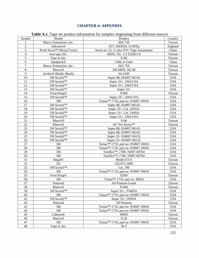
225
CHAPTER 4: APPENDIX
Table A.1. Tape set product information for samples originating from different sources Sample Brand Product Country
1 Marcy Enterprises, Inc. MA 750 Taiwan
2 Advance® AT7, BS3924, 31/90Tp England
3 Work Saver™ (Royal Tools) Stock no. 55, 5 color PVC Tape Assortment China
4 tesa tape, Inc. 40201, No. 111 E52811A Taiwan
5 Tape It, Inc. E-60 Taiwan
6 Qualpack® 1346, 6-Color China
7 Marcy Enterprises, Inc. MA 750 Taiwan
8 Manco® 200 MPH, AE-66 Taiwan
9 Archer® (Radio Shack) 64-2349 Taiwan
10 3M Scotch™ Super 88, 054007-06143 USA
11 3M Scotch™ Super 33+, 10414 NA USA
12 3M Scotch™ Super 33+, 10455 NA USA
13 3M Scotch™ Super 33+ USA
14 Frost King® ET60 Taiwan
15 3M Scotch™ Super 33+, 10455 NA USA
16 3M Tartan™ 1710, part no. 054007 49656 USA
17 3M Scotch™ Super 88, 054007-06143 USA
18 3M Scotch™ Super 33+, Cat. 195NA USA
19 3M Scotch™ Super 33+, Cat. 194NA USA
20 3M Scotch™ Super 33+, 10414 NA USA
21 Manco® P-66 Taiwan
22 Manco® 667 Pro Series™ Taiwan
23 3M Scotch™ Super 88, 054007-06143 USA
24 3M Scotch™ Super 88, 054007-06143 USA
25 3M Scotch™ Super 33+ 054007-06132 USA
26 3M Scotch™ Super 33+ 054007-06132 USA
27 3M Tartan™ 1710, part no. 054007 49656 USA
28 3M Tartan™ 1710, part no. 054007 49656 USA
29 3M Temflex™, 1700, 54007-69764 USA
30 3M Temflex™, 1700, 54007-69764 USA
31 Regal® Model ET-6 Taiwan
32 GE GE2472-3DD Taiwan
33 3M Scotch™ Cat. 190 USA
34 3M Tartan™ 1710, part no. 054007 49656 USA
35 Frost King® ET60 Taiwan
36 3M Tartan™ 1710, part no. 49656 USA
37 National All-Purpose Grade Taiwan
38 Manco® P-660 Taiwan
39 3M Scotch™ Super 33+, 3744NA USA
40 3M Tartan™ 1710, part no. 054007 49656 USA
41 3M Scotch™ Super 33+, 200NA USA
42 National All-Purpose Taiwan
43 3M Tartan™ 1710, part no. 054007 49656 USA
44 3M Tartan™ 1710, part no. 054007 49656 USA
45 Calterm® 49605 Taiwan
46 Manco® P-20 Taiwan
47 3M Tartan™ 1710, part no. 054007 49656 USA
48 Tape It, Inc. 36-T USA
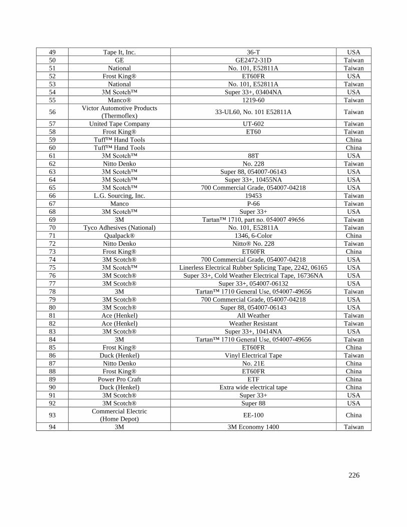
226
49 Tape It, Inc. 36-T USA
50 GE GE2472-31D Taiwan
51 National No. 101, E52811A Taiwan
52 Frost King® ET60FR USA
53 National No. 101, E52811A Taiwan
54 3M Scotch™ Super 33+, 03404NA USA
55 Manco® 1219-60 Taiwan
56 Victor Automotive Products
(Thermoflex) 33-UL60, No. 101 E52811A Taiwan
57 United Tape Company UT-602 Taiwan
58 Frost King® ET60 Taiwan
59 Tuff™ Hand Tools China
60 Tuff™ Hand Tools China
61 3M Scotch™ 88T USA
62 Nitto Denko No. 228 Taiwan
63 3M Scotch™ Super 88, 054007-06143 USA
64 3M Scotch™ Super 33+, 10455NA USA
65 3M Scotch™ 700 Commercial Grade, 054007-04218 USA
66 L.G. Sourcing, Inc. 19453 Taiwan
67 Manco P-66 Taiwan
68 3M Scotch™ Super 33+ USA
69 3M Tartan™ 1710, part no. 054007 49656 Taiwan
70 Tyco Adhesives (National) No. 101, E52811A Taiwan
71 Qualpack® 1346, 6-Color China
72 Nitto Denko Nitto® No. 228 Taiwan
73 Frost King® ET60FR China
74 3M Scotch® 700 Commercial Grade, 054007-04218 USA
75 3M Scotch™ Linerless Electrical Rubber Splicing Tape, 2242, 06165 USA
76 3M Scotch® Super 33+, Cold Weather Electrical Tape, 16736NA USA
77 3M Scotch® Super 33+, 054007-06132 USA
78 3M Tartan™ 1710 General Use, 054007-49656 Taiwan
79 3M Scotch® 700 Commercial Grade, 054007-04218 USA
80 3M Scotch® Super 88, 054007-06143 USA
81 Ace (Henkel) All Weather Taiwan
82 Ace (Henkel) Weather Resistant Taiwan
83 3M Scotch® Super 33+, 10414NA USA
84 3M Tartan™ 1710 General Use, 054007-49656 Taiwan
85 Frost King® ET60FR China
86 Duck (Henkel) Vinyl Electrical Tape Taiwan
87 Nitto Denko No. 21E China
88 Frost King® ET60FR China
89 Power Pro Craft ETF China
90 Duck (Henkel) Extra wide electrical tape China
91 3M Scotch® Super 33+ USA
92 3M Scotch® Super 88 USA
93 Commercial Electric
(Home Depot) EE-100 China
94 3M 3M Economy 1400 Taiwan
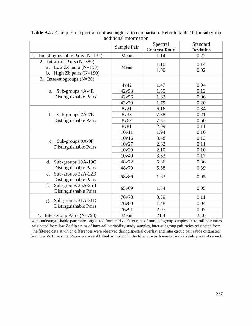
227
Table A.2. Examples of spectral contrast angle ratio comparison. Refer to table 10 for subgroup
additional information
Sample Pair Spectral
Contrast Ratio
Standard
Deviation
1. Indistinguishable Pairs (N=132) Mean 1.14 0.22
2. Intra-roll Pairs (N=380)
a. Low Zc pairs (N=190)
b. High Zb pairs (N=190)
Mean 1.10
1.00
0.14
0.02
3. Inter-subgroups (N=20)
a. Sub-groups 4A-4E
Distinguishable Pairs
4v42 1.47 0.04
42v53 1.55 0.12
42v56 1.62 0.06
42v70 1.79 0.20
b. Sub-groups 7A-7E
Distinguishable Pairs
8v21 6.16 0.34
8v38 7.88 0.21
8v67 7.37 0.50
8v81 2.09 0.11
c. Sub-groups 9A-9F
Distinguishable Pairs
10v11 1.94 0.10
10v16 3.48 0.13
10v27 2.62 0.11
10v39 2.10 0.10
10v40 3.63 0.17
d. Sub-groups 19A-19C
Distinguishable Pairs
48v72 5.36 0.36
48v79 5.58 0.39
e. Sub-groups 22A-22B
Distinguishable Pairs 58v86 1.63 0.05
f. Sub-groups 25A-25B
Distinguishable Pairs 65v69 1.54 0.05
g. Sub-groups 31A-31D
Distinguishable Pairs
76v78 3.39 0.11
76v80 1.48 0.04
76v91 2.07 0.07
4. Inter-group Pairs (N=794) Mean 21.4 22.0 Note: Indistinguishable pair ratios originated from mid Zc filter runs of intra-subgroup samples, intra-roll pair ratios
originated from low Zc filter runs of intra-roll variability study samples, inter-subgroup pair ratios originated from
the filtered data at which differences were observed during spectral overlay, and inter-group pair ratios originated
from low Zc filter runs. Ratios were established according to the filter at which worst-case variability was observed.
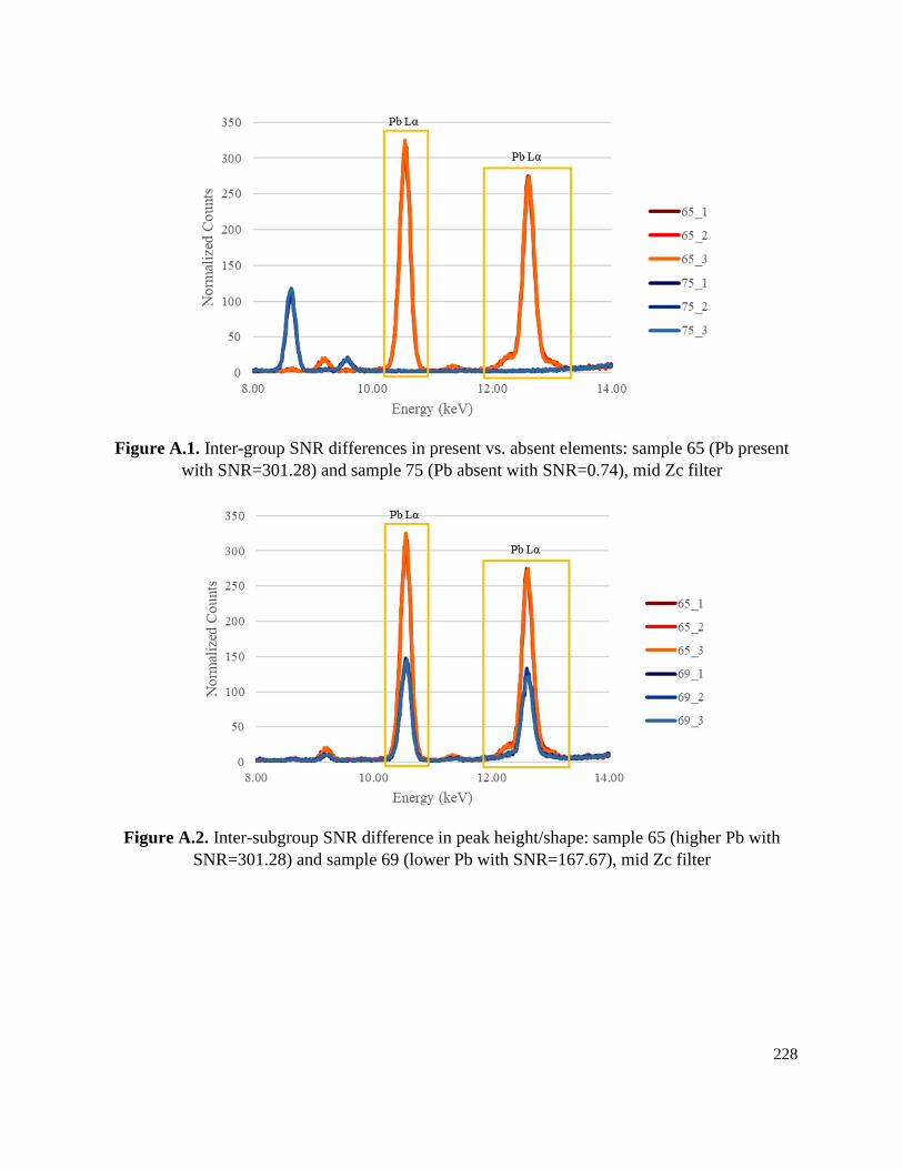
228
Figure A.1. Inter-group SNR differences in present vs. absent elements: sample 65 (Pb present
with SNR=301.28) and sample 75 (Pb absent with SNR=0.74), mid Zc filter
Figure A.2. Inter-subgroup SNR difference in peak height/shape: sample 65 (higher Pb with
SNR=301.28) and sample 69 (lower Pb with SNR=167.67), mid Zc filter
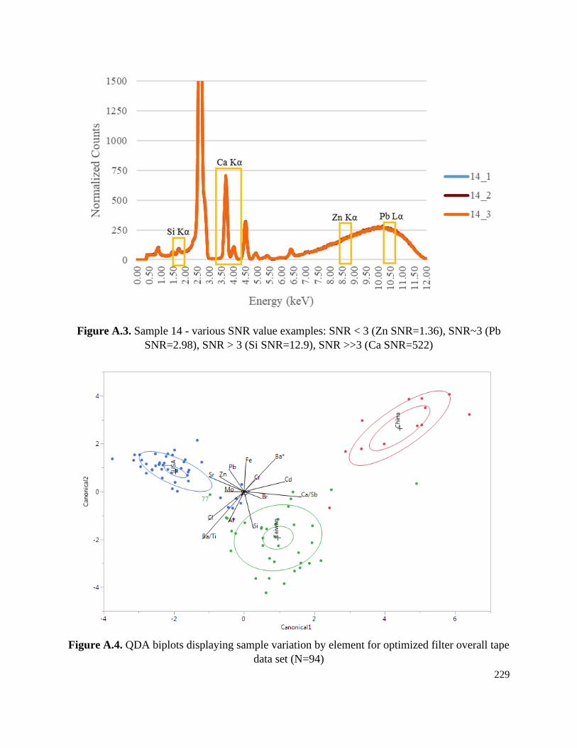
229
Figure A.3. Sample 14 - various SNR value examples: SNR < 3 (Zn SNR=1.36), SNR~3 (Pb
SNR=2.98), SNR > 3 (Si SNR=12.9), SNR >>3 (Ca SNR=522)
Figure A.4. QDA biplots displaying sample variation by element for optimized filter overall tape
data set (N=94)
230
VI. OVERALL CONCLUSIONS AND FUTURE WORK
The forensic fracture fit discipline has a vast and well-established case report foundation,
providing documentation of the value these evidential linkages have supplied to forensic casework
dating back as far as the 1700s.13 The physical fit research base continues to evolve to meet the
modern demands faced by the forensic field. Many different approaches have been taken to study
physical fits including, generally, case reports, fractography or qualitative-based studies, and
quantitative-based studies. Case reports are typically published by forensic practitioners and allow
the authors to document and share their casework experiences with others in the field, providing
innovative methodology for unusual material types5,6 and assisting researchers in understanding
the prevalence of certain items in casework. Fractography studies attempt to shed light into the
nature of fractures of specific materials to provide qualitative features that examiners may
incorporate in their physical fit assessments to demonstrate either alignment or inconsistency
between two items. Quantitative-based studies have expanded recently, with studies emerging for
performance assessment through examiner error rates during physical fit assessments,21,22 score-
based reporting and quantitative assessment through the score likelihood ratio,14 statistical
interpretations through attempts at populational frequency studies,23,24 and most recently the
expansion of automated algorithms for more objective fracture fit application and support.25,26
Growth in these quantitative aspects aims to substantiate the scientific validity of one of the oldest
and seemingly straightforward forensic analyses, advocating for the discipline in response to NAS,
PCAST, ASA, and NIST-OSAC recommendations8–11.
To attribute to the need for quantitative approaches to physical fit examinations, the pilot inter-
laboratory study conducted in this thesis was designed to take steps towards validation of
systematic, score-based ESS methodology previously developed by Prusinowski et al.14 The ESS
values, comparison edge qualifiers, and overall examiner conclusions from 16 participants were
assessed for inter-examiner agreement, examiner error rates, variance from consensus means, and
survey feedback to facilitate future adoption of the method to their laboratories. Overall, inter-
examiner agreement with reporting ESS scores within 20% of the mean consensus values was
observed, with participants accuracy ranging from 88 to 100%. Moreover, the inter-laboratory
study highlighted the utility of the ESS score method to enhance future physical fit practice in
several aspects including increased objectivity, consensus between examiners, peer-review
process, proficiency testing, and strengthened scientific reliability.
A thorough review of participant scrim templates, examination notes, and feedback left within the
post-study survey revealed three main observations. First, those participants that did not participate
in formal method training through either the in-person method presentation or teleconference
tended to exhibit statistically significant score differences from the consensus, pre-distribution
mean ESS. This was shown through results of the Dunnett’s test as well as distribution of scores.
Second, variance was observed in how participants interpreted a featureless or distorted scrim bin
for ESS assignment. While some assigned a “0” binary classifier to those areas to signify they had
interpreted it as a non-matching, inconsistent bin, others assigned a “1” binary classifier to indicate
the bin was interpreted as a matching, consistent area. When facing this discrepancy, some
231
examiners recommended the option of an “inconclusive” qualifier for scrim bins. The third
observation was an apparent misunderstanding in application of the comparison edge qualifier.
Expected ranges were set for ESS based on the assignment of comparison edge qualifiers
according to previously determined score likelihood ratios (SLRs)14, and many examiners did not
provide qualifiers that were reasonable for certain ESS ranges. As a result, future work on
expanded inter-laboratory studies will include more in-depth, mandatory training as a pre-requisite
to participation, in addition to incorporation of the inconclusive scrim bin criteria. In addition,
future work will include the application of a linear mixed model fit by restricted maximum
likelihood (REML) to inter-laboratory study results as an input for Bayesian models to provide
credible intervals for variation between examiners.
Along with the expansion of the duct tape ESS project, the application of the ESS to clothing items
represents the first time a quantitative, score-based method of physical fit assessment has been
applied to textile materials. The methodology allowed for quantitative assessment of examiner
performance, and both the hand-torn and stabbed sample sets presented low error rates with
accuracies ranging from 85-100% depending on textile item. One of the most significant
discoveries in this study was the impact a fabric composition and construction type may have in
the suitability of a physical fit. Lower accuracy rates were observed for items of either polyester
composition (Item D) or jersey knit construction (Item E) for the hand-torn set, while woven, non-
polyester items exhibited higher accuracy rates. This was attributed to higher distortion in the
polyester or jersey knit items, as was also observed in a preliminary set of 100 jersey knit, 100%
polyester comparison pairs, where unacceptable high error rates demonstrated the challenges of
evaluation of fracture fits on these types of textiles. For the stabbed sample set, it was observed
that patterned materials (Items C and E) exhibited higher accuracy rates than solid-colored items.
This was attributed to the added potential of pattern alignment (or misalignment) on items
presenting otherwise “featureless” edges due to the stabbing separation mechanism.
Also, another relevant aspect of this study was the identification, documentation, and description
of physical features that can lead to future standardization of examination protocols. Further
analysis of examiner notes revealed two main methodology discrepancies dealing with treatment
of gaps within a sample as well as treatment of inconsistent fracture edge length between two
items. Regardless of examiner discrepancies, only 12 misclassifications were observed across the
entire data set. While one false positive was observed, and later realized as an observation error by
the examiner during peer review, the remaining 11 misclassifications consisted of false negative
and inconclusive results. These results are less detrimental to casework as negative or inconclusive
samples would typically be subject to further testing according to a forensic laboratory’s associated
analytical scheme.
The textile fracture study provided an important foundation from which future textile physical fit
research may expand, as it established preliminary ESS data on various textile compositions,
constructions, and separation methods. In addition, study data revealed that due to high
disagreement rates between examiners, certain textiles may be unsuitable for physical fit analysis
232
if lacking distinctive characteristics beyond general characteristics. The jersey knit construction
and 100% polyester composition demonstrated to be unsuitable for fracture fit analysis as
deformations lead to high rates of misclassification. These results raise awareness as to the need
to further evaluate the effect of other textile types on error rates. Future work will include studies
of expanded textile factors such as additional compositions, constructions, and external factors
such as degree of wear, in order to determine if modifications to the textile ESS criteria are needed.
In addition, future work and expanded datasets will assist in the fine-tuning of the proposed verbal
interpretation scale based upon rarity ratio thresholds. Eventually, an inter-laboratory study is
recommended to validate the now developed textile ESS methodology.
In the absence of physical fits, it is critical for forensic examiners to have access to highly
discriminatory techniques for optimal utilization of the probative value of submitted evidence
items. This becomes especially critical on items such as electrical tape that are more prone to
deformation, with a lack of distinctive features on the fractured edges. As electrical tapes are
amorphous materials exhibiting enough physical fit variability to cause the FBI to modify their
physical match protocols,15 it is important that efficient methods are available to the examiner
upon continued chemical analysis. The XRF method presented in this work provides an additional
tool to traditional electrical tape chemical analysis.
The XRF study aimed to expand previous work into electrical tape XRF method development.18
The optimization process described through this study suggests proper parameters for XRF
electrical tape analysis, and the additional experiments using those optimized parameters provides
a model of the key factors and potential interferences to assess when attempting to adapt this
method for use in other forensic laboratories. This experimentation established that this technique
is well suited for quick screening with accuracy and discrimination over time, precision,
sensitivity, and selectivity. This study also highlighted the high inter-sample variability and low
intra-sample variability of electrical tape backings as characterized through the optimized XRF
method. Further, results of the study support the application of spectral contrast angle
interpretation to spectral comparison, as it has been demonstrated to be a useful tool for supporting
examiner opinion and complementing spectral overlay comparisons. Future work using additional
tape datasets is recommended to test these findings further and evaluate the potential adoption of
contrast ratios comparisons to casework.
Physical fits are a complex research topic. Many factors influence the resulting fracture pattern
and vary by material type. To name a few, the force of the fracture, directionality, object used to
impart the break, manipulation following the breaking event, and even temperature may influence
the resulting fracture edge features. However, this inherent randomization of physical fit events is
precisely what adds significance to their occurrence. Therefore, it is critical experimental,
quantitative, and systematic research bases be established for a wide variety of material types so
that the strength of these potential evidential linkages is best represented and upheld in the court
setting. In doing so, it must be stressed that physical fit examinations can never be truly objective,
as the examiner’s expert opinion is an essential input in the overall assessment. Although, with
added quantitative interpretation, statistical capabilities, and automated algorithm support, the high
233
associative power of physical fit examinations can be more transparently and credibly validated
instances of forensic evidence.
This thesis research represents important steps towards meeting these means. By organizing and
summarizing the vast physical fit research basis (Chapter 1), an understanding of the strength and
history of the discipline is shared with the forensic community and beyond. The pilot inter-
laboratory study of the duct tape ESS method (Chapter 2) provides the first step into the
implementation process, as examiner feedback and modification are crucial aspects to optimizing
the methodology. As the long-term goals of our research group include expanding the ESS
technique into multiple material types of trace evidence interest, the textile fracture study (Chapter
3) represents the novel application of the methodology to textile materials. Finally, in order to
account for amorphous materials in which physical fits may not be feasible due to a lack of
distinctive features, an XRF technique has been optimized for implementation into forensic
laboratories for the rapid, highly discriminatory analysis of electrical tape backing samples. A
systematic method for spectral comparison was also proposed and evaluated to help examiners in
the decision-making process (Chapter 4). Future work will expand upon the groundwork laid for
the growth of the physical fit discipline through this research.
234
VII. OVERALL REFERENCES
These references correspond to citations on the Overall Introduction (Section I) and Overall
Conclusions/Future Work Sections (Section VI).
1. American Society of Trace Evidence Examiners (ASTEE). ASTEE Trace 101. 2018 [accessed
2018 Dec 12]. http://www.asteetrace.org/
2. Gummer T, Walsh K. Matching vehicle parts back to the vehicle: a study of the process.
Forensic Science International. 1996;82:89–97. doi:10.1016/0379-0738(96)01970-6
3. Jayaprakash PT. Practical relevance of pattern uniqueness in forensic science. Forensic
Science International. 2013;231:403.e1-403.e16. doi:10.1016/j.forsciint.2013.05.028
4. Ryland S, Houck MM. Only Circumstantial Evidence. In: Houck MM, editor. Mute
Witnesses: Trace Evidence Analysis. San Diego, CA: Academic Press; 2001. p. 117–137.
5. Perper JA, Prichard W, McCommons P. Matching the Lost Skin of a Homicide Suspect.
Forensic Science International. 1985;29:77–82.
6. Bisbing RE, Willmer JH, LaVoy TA, Berglund JS. A Fingernail Identification. AFTE Journal.
1980;12(1):27–28.
7. Scientific Working Group on Materials Analysis (SWGMAT). A 2012 Survey Regarding the
Status of Forensic Tape Analysis. 2012.
8. Gross S. NIST-OSAC Materials (Trace) Subcommittee, physical fit task group, 2020 physical
fit survey.
9. National Academy of Sciences (NAS). Strengthening Forensic Science in the United States: A
Path Forward. 2009. doi:0.17226/12589
10. President’s Council of Advisors on Science and Technology. Forensic Science in Criminal
Courts: Ensuring Scientific Validity of Feature-Comparison Methods. 2016.
11. American Statistical Association. American Statistical Association Position on Statistical
Statements for Forensic Evidence. [accessed 2019 Jan 30].
https://www.amstat.org/asa/files/pdfs/POL-ForensicScience.pdf
12. {US Supreme Court}. Daubert vs Merrell Dow Pharmaceuticals, Inc. 509 U.S. 579 (1993).
JUSTIA US Supreme Couts. 1993.
13. Gehl R, Plecas D. Chapter 1: Introduction. In: Introduction to Criminal Investigation:
Processes, Practices and Thinking. New Westminster, BC: Justice Institute of British Columbia;
2016. p. 1–10.
14. Prusinowski M, Brooks E, Trejos T. Development and validation of a systematic approach
for the quantitative assessment of the quality of duct tape physical fits. Forensic Science
International. 2020;307.
235
15. Bradley MJ, Gauntt JM, Mehltretter AH, Lowe PC, Wright DM. A Validation Study for
Vinyl Electrical Tape End Matches. Journal of Forensic Sciences. 2011;56(3):606–611.
doi:10.1111/j.1556-4029.2011.01736.x
16. Kee TG. The Characterization of PVC Adhesive Tape. In: Proceedings of International
Symposium on the Analysis and Identification of Polymers. FBI Academy, Quantico, VA; 1984.
p. 77–85.
17. Keto RO. Forensic characterization of black polyvinyl chloride electrical tape. Crime
Laboratory Digest. 1984;11(4).
18. Prusinowski M, Mehltretter A, Martinez-Lopez C, Almirall J, Trejos T. Assessment of the
utility of X-ray Fluorescence for the chemical characterization and comparison of black electrical
tape backings. Forensic Chemistry. 2019;13(January):100146. doi:10.1016/j.forc.2019.100146
19. Martinez-Lopez C, Trejos T, Mehltretter AH, Almirall JR. Elemental analysis and
characterization of electrical tape backings by LA-ICP-MS. Forensic Chemistry. 2017;4:96–107.
doi:10.1016/j.forc.2017.03.003
20. Mehltretter AH, Bradley MJ, Wright DM. Analysis and discrimination of electrical tapes:
Part II. Backings. Journal of Forensic Sciences. 2011;56(6):1493–1504. doi:10.1111/j.1556-
4029.2011.01873.x
21. Bradley MJ, Keagy RL, Lowe PC, Rickenbach MP, Wright DM, LeBeau MA. A validation
study for duct tape end matches. Journal of Forensic Sciences. 2006;51(3):504–508.
doi:10.1111/j.1556-4029.2006.00106.x
22. Christensen AM, Sylvester AD. Physical Matches of Bone, Shell and Tooth Fragments: A
Validation Study. Journal of Forensic Sciences. 2008;53(3):694–698. doi:10.1111/j.1556-
4029.2008.00705.x
23. Lograsso BK. Physical Matching of Metals: Grain Orientation Association at Fracture Edge.
Journal of Forensic Sciences. 2015;60(S1):S66–S75. doi:10.1111/1556-4029.12607
24. Stone RS. A Probabilistic Model of Fractures in Brittle Metals. AFTE Journal.
2004;36(4):297–301.
25. Yekutieli Y, Shor Y, Wiesner S, Tsach T. Physical Matching Verification. Final Report to
United States Department of Justice on Grant 2005-IJ-R-051; National Criminal Justice
Reference Service: Rockville, MD. 2012.
26. Ristenpart W, Tulleners FA, Alfter A. Quantitative Algorithm for the Digital Comparison of
Torn Duct Tape. Final Report to the National Institute of Justice Grant 2013-R2-CX-K009;
University of California at Davis: Davis, CA. 2017.
Related Documents


![Maxillofacial Fractures due to Falls: does Fall …FISS, and fracture location. Data were expressed as mean and standard deviation (M [SD]). Statistical significance was determined](https://static.cupdf.com/doc/110x72/5f2b65d86e4fe637f359b8da/maxillofacial-fractures-due-to-falls-does-fall-fiss-and-fracture-location-data.jpg)