STATA 13 - London School of Hygiene & Tropical Medicine · 1 INTRODUCTION Versions of STATA STATA offers several different versions of their software. Each has different capabilities

0

STATA 13 INTRODUCTION

Catherine McGowan & Elaine Williamson LONDON SCHOOL OF HYGIENE & TROPICAL MEDICINE | DECEMBER 2013

CONTENTS

INTRODUCTION ....................................................................................................................................................... 1

Versions of STATA ................................................................................................................................................. 1

OPENING STATA....................................................................................................................................................... 1

THE STATA SCREEN .............................................................................................................................................. 2

OPENING FILES IN STATA ................................................................................................................................... 3

Opening STATA Format Files............................................................................................................................. 3

Opening Other Format Files ............................................................................................................................... 3

DATA ENTRY ............................................................................................................................................................. 4

Adding values .......................................................................................................................................................... 4

Modifying variable names and labels................................................................................................................. 4

Saving your data ..................................................................................................................................................... 4

Exploring data ........................................................................................................................................................ 4

Browsing through your data ........................................................................................................................... 4

Sorting data ......................................................................................................................................................... 5

The ‘DESCRIBE’ command ............................................................................................................................. 5

The ‘CODEBOOK’ command .......................................................................................................................... 5

The ‘SUMMARIZE’ command ....................................................................................................................... 6

The ‘TABULATE’ command ........................................................................................................................... 7

DATA MANAGEMENT ........................................................................................................................................... 8

Creating value labels ............................................................................................................................................. 8

Applying a value label to an existing variable ............................................................................................. 8

Creating a new categorical variable from a continuous variable ................................................................ 9

Changing contents of an existing variable ....................................................................................................... 9

Dropping a variable .............................................................................................................................................. 11

Keeping variables .................................................................................................................................................. 11

DATA ANALYSIS ...................................................................................................................................................... 11

Confidence intervals ............................................................................................................................................. 11

Confidence interval (mean) ........................................................................................................................... 11

Confidence interval (median) ........................................................................................................................ 11

Confidence interval (proportion) .................................................................................................................12

Confidence interval (difference in proportions) .......................................................................................12

T-tests ...................................................................................................................................................................... 13

One sample t-test ............................................................................................................................................. 13

Two sample t-test............................................................................................................................................. 13

Paired t-test ...................................................................................................................................................... 14

Chi-squared and Fisher’s exact test................................................................................................................. 14

Analysis of variance (ANOVA) ......................................................................................................................... 14

Pearson correlation ............................................................................................................................................... 15

Linear regression ................................................................................................................................................... 15

DATA VISUALISATION ......................................................................................................................................... 16

Continuous variable (Histogram) ..................................................................................................................... 16

Graph Editor ...................................................................................................................................................... 16

Continuous variable (Normal plot) .................................................................................................................. 17

Categorical variable (Bar chart) ........................................................................................................................ 17

Two continuous variables (Scatterplot) .......................................................................................................... 17

Adding a best fit line ........................................................................................................................................ 17

DO FILES ..................................................................................................................................................................... 18

LOG FILES ..................................................................................................................................................................19

THE ‘HELP’ COMMAND .......................................................................................................................................19

THE ‘SEARCH’ COMMAND .................................................................................................................................19

THE ‘FINDIT’ COMMAND ....................................................................................................................................19

1

INTRODUCTION

Versions of STATA

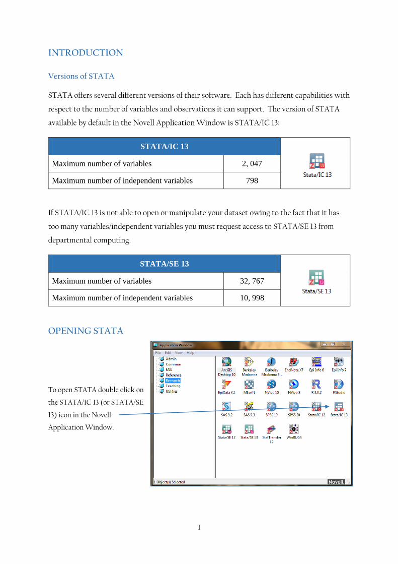
STATA offers several different versions of their software. Each has different capabilities with

respect to the number of variables and observations it can support. The version of STATA

available by default in the Novell Application Window is STATA/IC 13:

STATA/IC 13

Maximum number of variables 2, 047

Maximum number of independent variables 798

If STATA/IC 13 is not able to open or manipulate your dataset owing to the fact that it has

too many variables/independent variables you must request access to STATA/SE 13 from

departmental computing.

STATA/SE 13

Maximum number of variables 32, 767

Maximum number of independent variables 10, 998

OPENING STATA

To open STATA double click on

the STATA/IC 13 (or STATA/SE

13) icon in the Novell

Application Window.

2

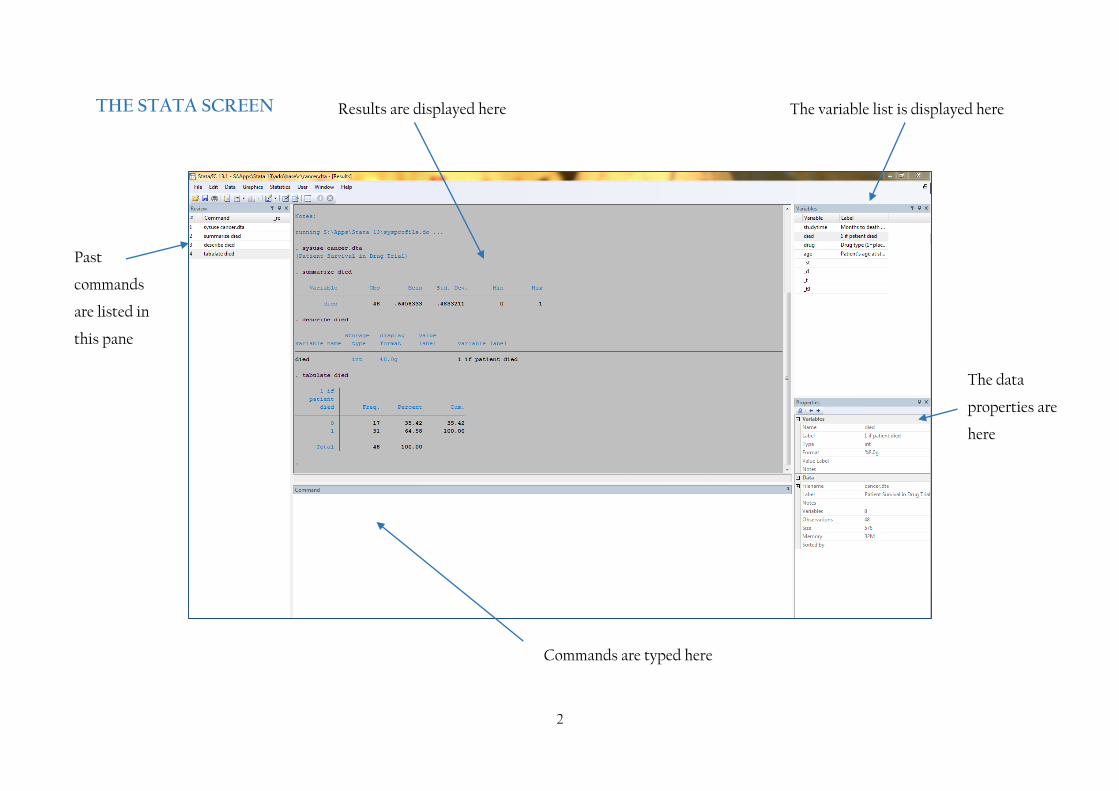
THE STATA SCREEN

Past

commands

are listed in

this pane

Results are displayed here The variable list is displayed here

The data

properties are

here

Commands are typed here

3

OPENING FILES IN STATA

Opening STATA Format Files

STATA files have the file extension .dta. To open a STATA format data file in STATA:

1. Open STATA and select FILE, then OPEN.

2. Browse to your .dta file and click OPEN.

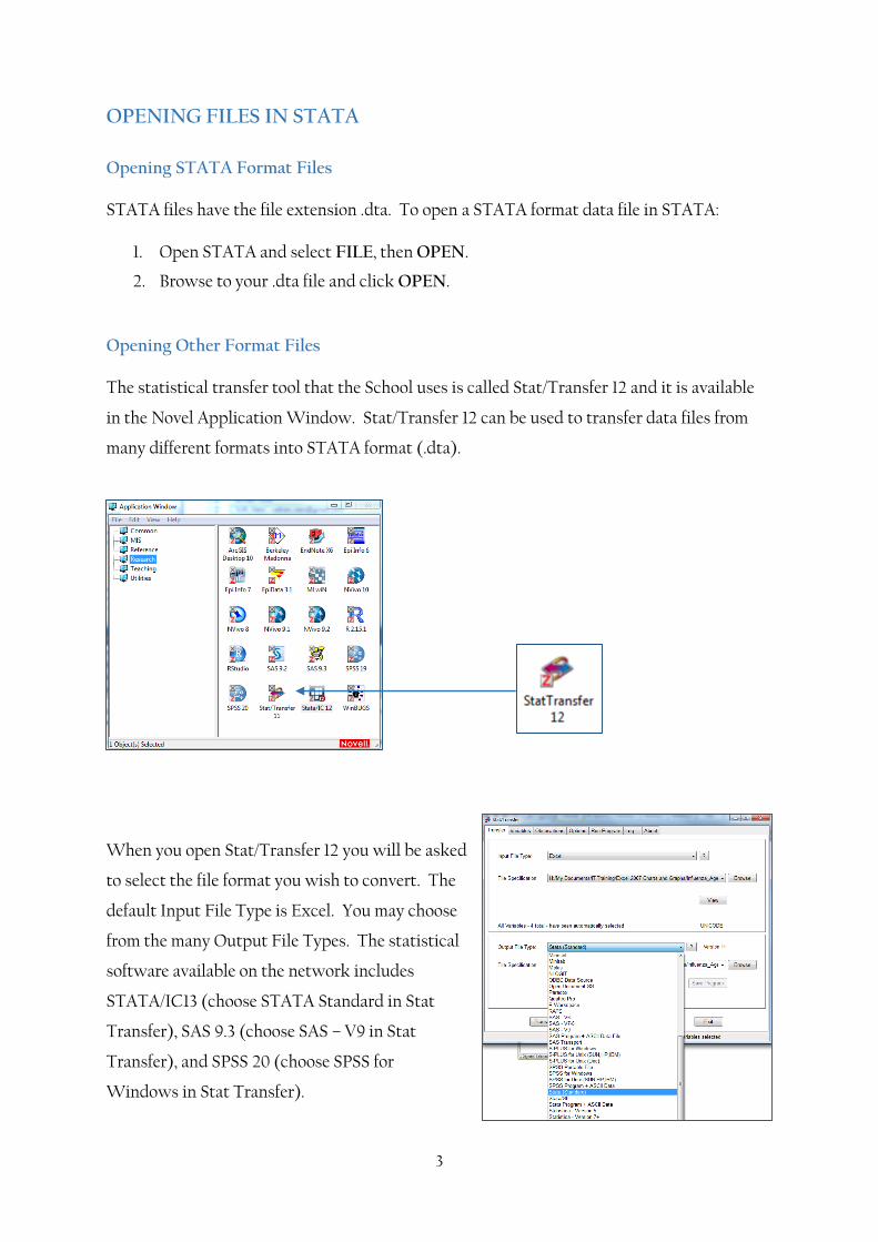
Opening Other Format Files

The statistical transfer tool that the School uses is called Stat/Transfer 12 and it is available

in the Novel Application Window. Stat/Transfer 12 can be used to transfer data files from

many different formats into STATA format (.dta).

When you open Stat/Transfer 12 you will be asked

to select the file format you wish to convert. The

default Input File Type is Excel. You may choose

from the many Output File Types. The statistical

software available on the network includes

STATA/IC13 (choose STATA Standard in Stat

Transfer), SAS 9.3 (choose SAS – V9 in Stat

Transfer), and SPSS 20 (choose SPSS for

Windows in Stat Transfer).

4

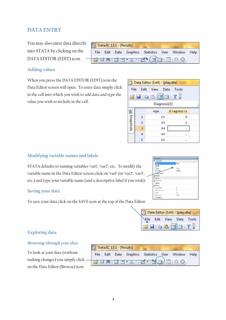
DATA ENTRY

You may also enter data directly

into STATA by clicking on the

DATA EDITOR (EDIT) icon.

Adding values

When you press the DATA EDITOR (EDIT) icon the

Data Editor screen will open. To enter data simply click

in the cell into which you wish to add data and type the

value you wish to include in the cell.

Modifying variable names and labels

STATA defaults to naming variables ‘var1’, ‘var2’, etc. To modify the

variable name in the Data Editor screen click on ‘var1’ (or ‘var2’, ‘var3’,

etc.) and type your variable name (and a descriptive label if you wish).

Saving your data

To save your data click on the SAVE icon at the top of the Data Editor.

Exploring data

Browsing through your data

To look at your data (without

making changes) you simply click

on the Data Editor (Browse) icon.

5

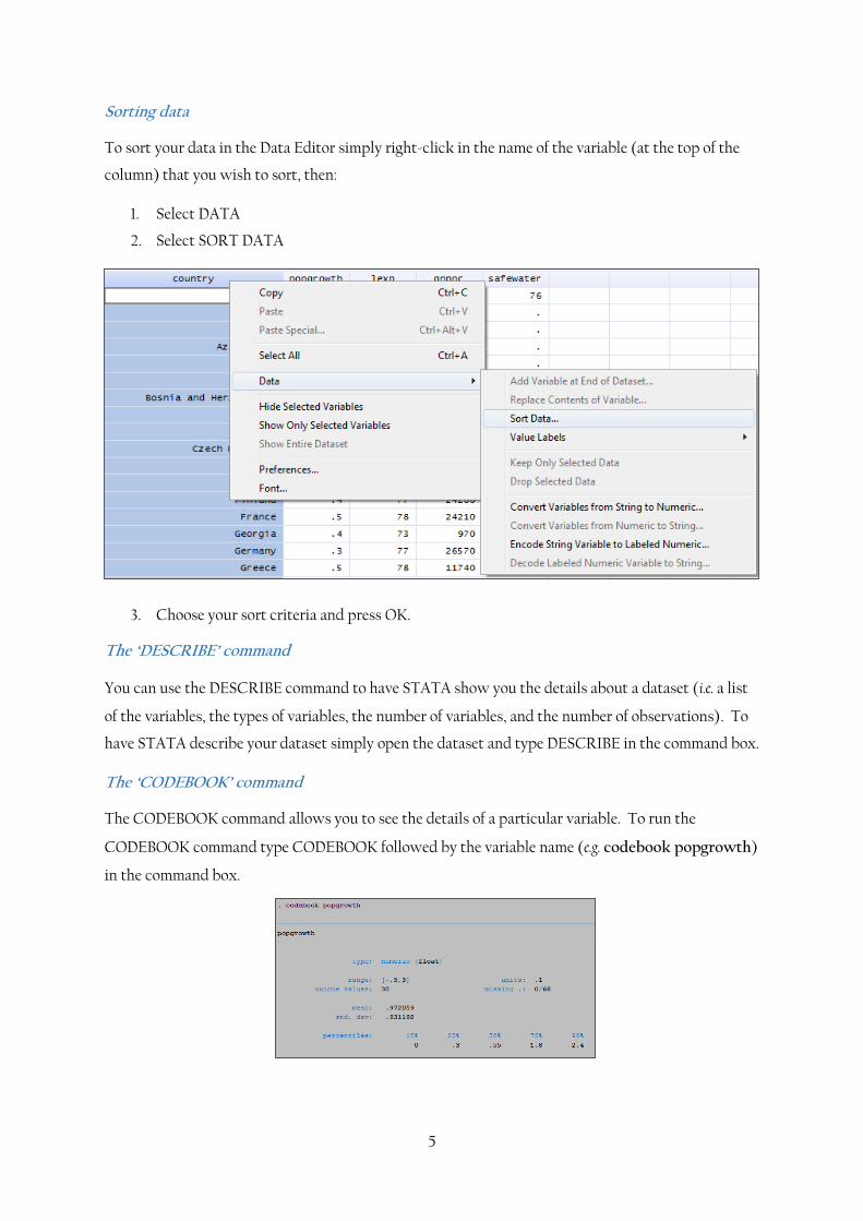
Sorting data

To sort your data in the Data Editor simply right-click in the name of the variable (at the top of the

column) that you wish to sort, then:

1. Select DATA

2. Select SORT DATA

3. Choose your sort criteria and press OK.

The ‘DESCRIBE’ command

You can use the DESCRIBE command to have STATA show you the details about a dataset (i.e. a list

of the variables, the types of variables, the number of variables, and the number of observations). To

have STATA describe your dataset simply open the dataset and type DESCRIBE in the command box.

The ‘CODEBOOK’ command

The CODEBOOK command allows you to see the details of a particular variable. To run the

CODEBOOK command type CODEBOOK followed by the variable name (e.g. codebook popgrowth)

in the command box.

6

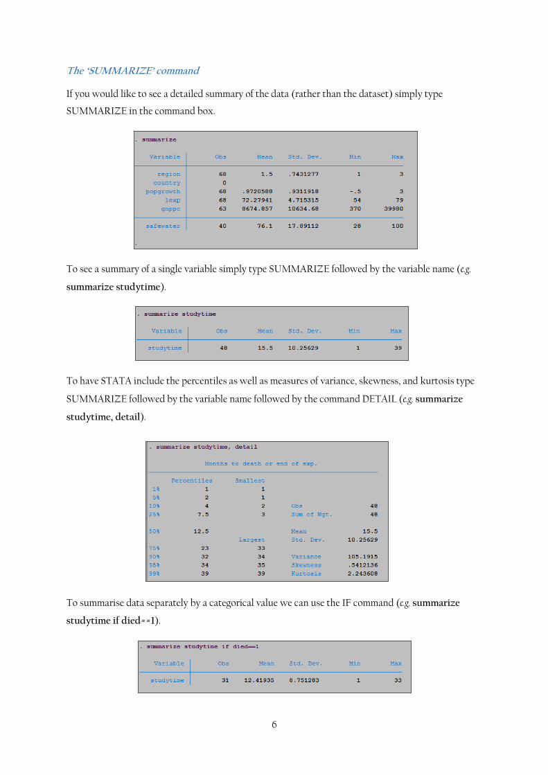
The ‘SUMMARIZE’ command

If you would like to see a detailed summary of the data (rather than the dataset) simply type

SUMMARIZE in the command box.

To see a summary of a single variable simply type SUMMARIZE followed by the variable name (e.g.

summarize studytime).

To have STATA include the percentiles as well as measures of variance, skewness, and kurtosis type

SUMMARIZE followed by the variable name followed by the command DETAIL (e.g. summarize

studytime, detail).

To summarise data separately by a categorical value we can use the IF command (e.g. summarize

studytime if died==1).

7

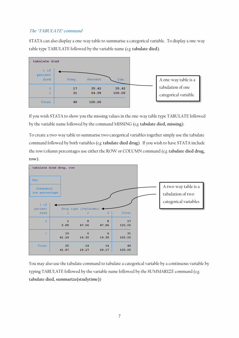
The ‘TABULATE’ command

STATA can also display a one-way table to summarise a categorical variable. To display a one-way

table type TABULATE followed by the variable name (e.g. tabulate died).

If you wish STATA to show you the missing values in the one-way table type TABULATE followed

by the variable name followed by the command MISSING (e.g. tabulate died, missing).

To create a two-way table to summarise two categorical variables together simply use the tabulate

command followed by both variables (e.g. tabulate died drug). If you wish to have STATA include

the row/column percentages use either the ROW or COLUMN command (e.g. tabulate died drug,

row).

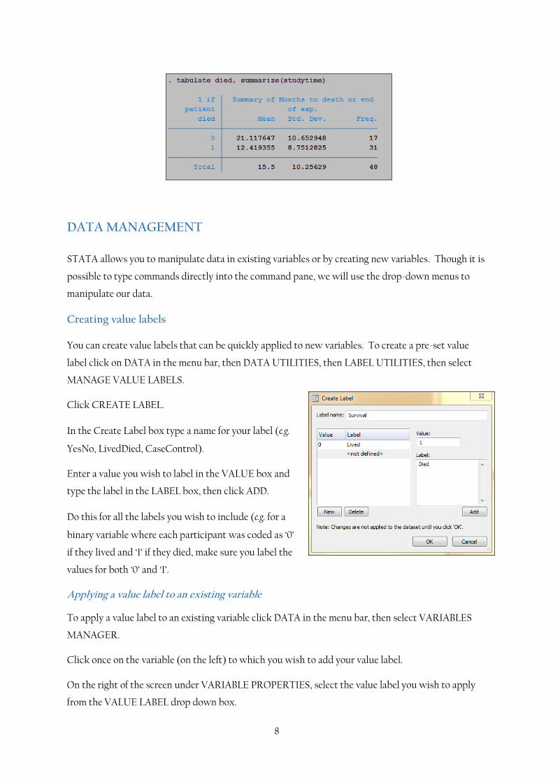
You may also use the tabulate command to tabulate a categorical variable by a continuous variable by

typing TABULATE followed by the variable name followed by the SUMMARIZE command (e.g.

tabulate died, summarize(studytime))

A one-way table is a

tabulation of one

categorical variable

A two-way table is a

tabulation of two

categorical variables

8

DATA MANAGEMENT

STATA allows you to manipulate data in existing variables or by creating new variables. Though it is

possible to type commands directly into the command pane, we will use the drop-down menus to

manipulate our data.

Creating value labels

You can create value labels that can be quickly applied to new variables. To create a pre-set value

label click on DATA in the menu bar, then DATA UTILITIES, then LABEL UTILITIES, then select

MANAGE VALUE LABELS.

Click CREATE LABEL.

In the Create Label box type a name for your label (e.g.

YesNo, LivedDied, CaseControl).

Enter a value you wish to label in the VALUE box and

type the label in the LABEL box, then click ADD.

Do this for all the labels you wish to include (e.g. for a

binary variable where each participant was coded as ‘0’

if they lived and ‘1’ if they died, make sure you label the

values for both ‘0’ and ‘1’.

Applying a value label to an existing variable

To apply a value label to an existing variable click DATA in the menu bar, then select VARIABLES

MANAGER.

Click once on the variable (on the left) to which you wish to add your value label.

On the right of the screen under VARIABLE PROPERTIES, select the value label you wish to apply

from the VALUE LABEL drop down box.

9

Click APPLY and open your data in your Data Browser to make sure the label has been applied.

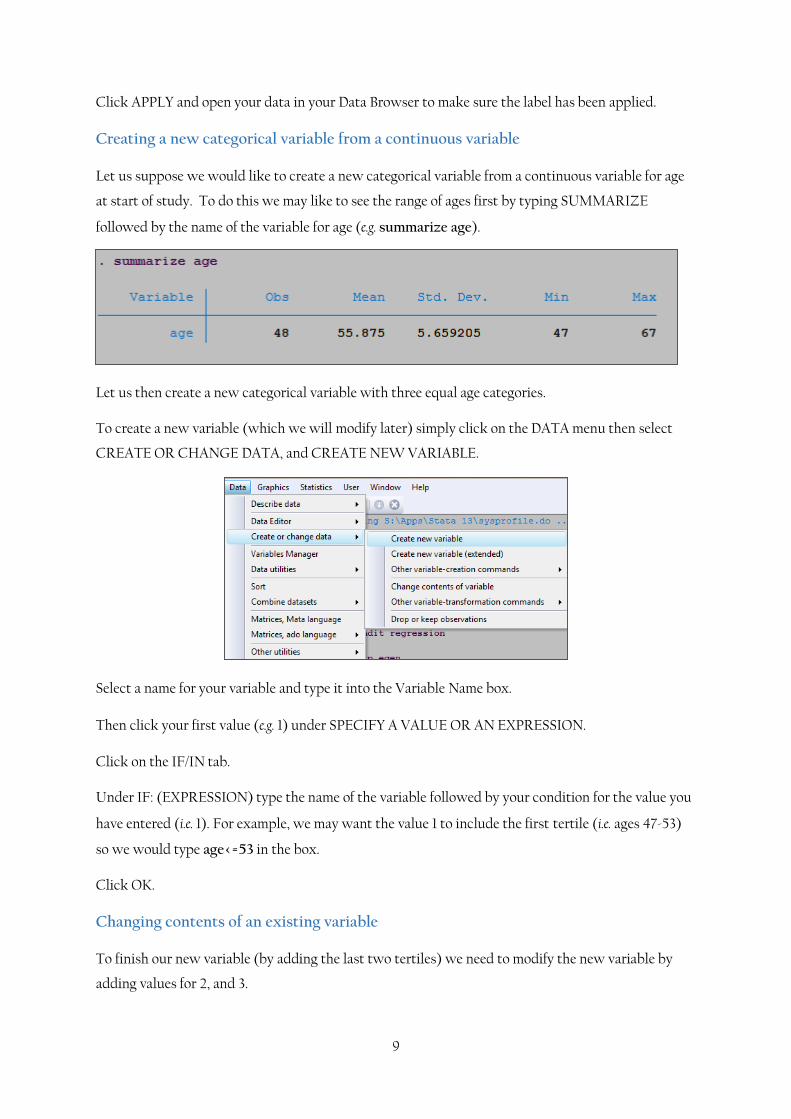
Creating a new categorical variable from a continuous variable

Let us suppose we would like to create a new categorical variable from a continuous variable for age

at start of study. To do this we may like to see the range of ages first by typing SUMMARIZE

followed by the name of the variable for age (e.g. summarize age).

Let us then create a new categorical variable with three equal age categories.

To create a new variable (which we will modify later) simply click on the DATA menu then select

CREATE OR CHANGE DATA, and CREATE NEW VARIABLE.

Select a name for your variable and type it into the Variable Name box.

Then click your first value (e.g. 1) under SPECIFY A VALUE OR AN EXPRESSION.

Click on the IF/IN tab.

Under IF: (EXPRESSION) type the name of the variable followed by your condition for the value you

have entered (i.e. 1). For example, we may want the value 1 to include the first tertile (i.e. ages 47-53)

so we would type age<=53 in the box.

Click OK.

Changing contents of an existing variable

To finish our new variable (by adding the last two tertiles) we need to modify the new variable by

adding values for 2, and 3.

10

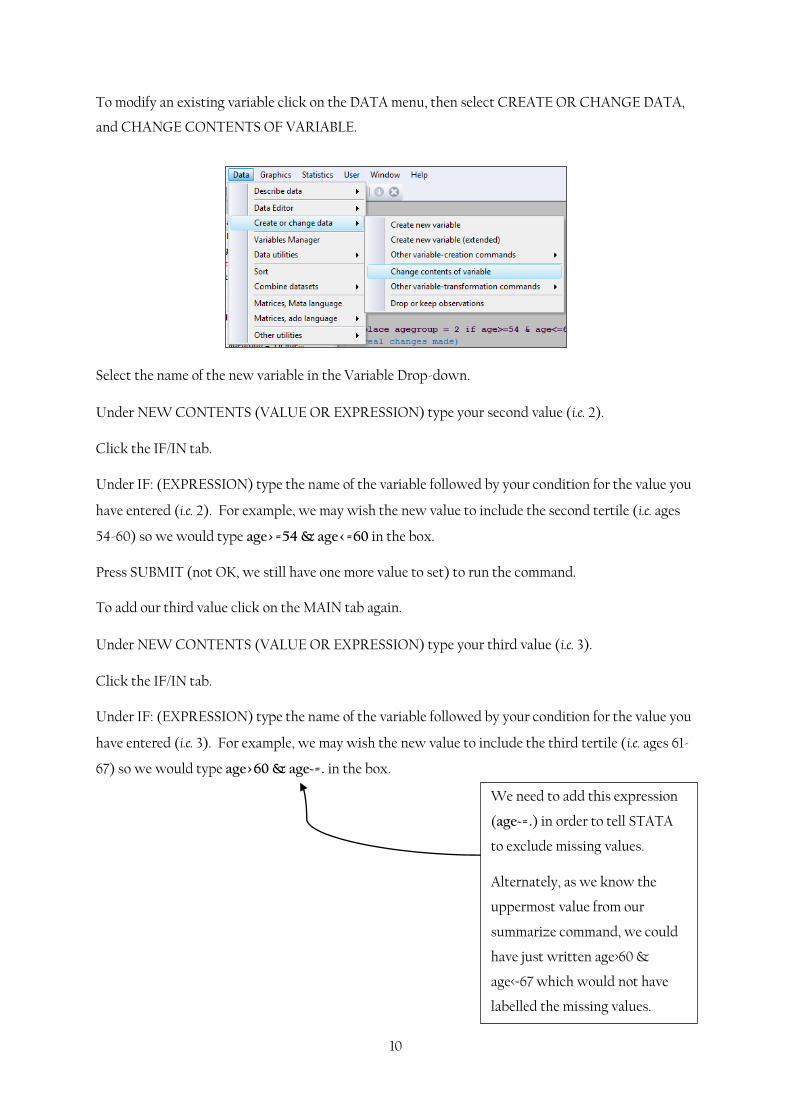
To modify an existing variable click on the DATA menu, then select CREATE OR CHANGE DATA,

and CHANGE CONTENTS OF VARIABLE.

Select the name of the new variable in the Variable Drop-down.

Under NEW CONTENTS (VALUE OR EXPRESSION) type your second value (i.e. 2).

Click the IF/IN tab.


have entered (i.e. 2). For example, we may wish the new value to include the second tertile (i.e. ages

54-60) so we would type age>=54 & age<=60 in the box.

Press SUBMIT (not OK, we still have one more value to set) to run the command.

To add our third value click on the MAIN tab again.

Under NEW CONTENTS (VALUE OR EXPRESSION) type your third value (i.e. 3).

Click the IF/IN tab.


have entered (i.e. 3). For example, we may wish the new value to include the third tertile (i.e. ages 61-

67) so we would type age>60 & age~=. in the box.

We need to add this expression

(age~=.) in order to tell STATA

to exclude missing values.

Alternately, as we know the

uppermost value from our

summarize command, we could

have just written age>60 &

age<=67 which would not have

labelled the missing values.

11

Dropping a variable

To drop a variable from a dataset simply type DROP followed by the name of the variable (e.g. drop

drug).

Keeping variables

If you have a dataset with many variables of which you only wish to keep a few, it might be easier to

use the KEEP command rather than the DROP command (e.g. keep studytime died drug age)

DATA ANALYSIS

STATA is capable of carrying out many different types of analyses. We will review only the

most basic commands below. For more complex analyses please refer to: An Introduction

to STATA for Health Researchers (Third Edition) by Svend Juul and Morten

Frydenberg (2010).

Alternately you can use the SEARCH or FINDIT commands to look for guidance.

Confidence intervals

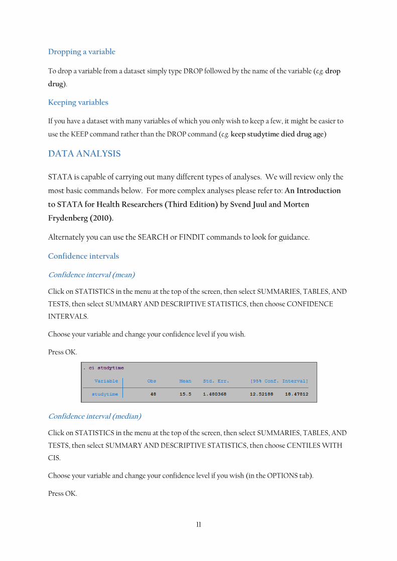
Confidence interval (mean)

Click on STATISTICS in the menu at the top of the screen, then select SUMMARIES, TABLES, AND

TESTS, then select SUMMARY AND DESCRIPTIVE STATISTICS, then choose CONFIDENCE

INTERVALS.

Choose your variable and change your confidence level if you wish.

Press OK.

Confidence interval (median)


TESTS, then select SUMMARY AND DESCRIPTIVE STATISTICS, then choose CENTILES WITH

CIS.

Choose your variable and change your confidence level if you wish (in the OPTIONS tab).

Press OK.

12

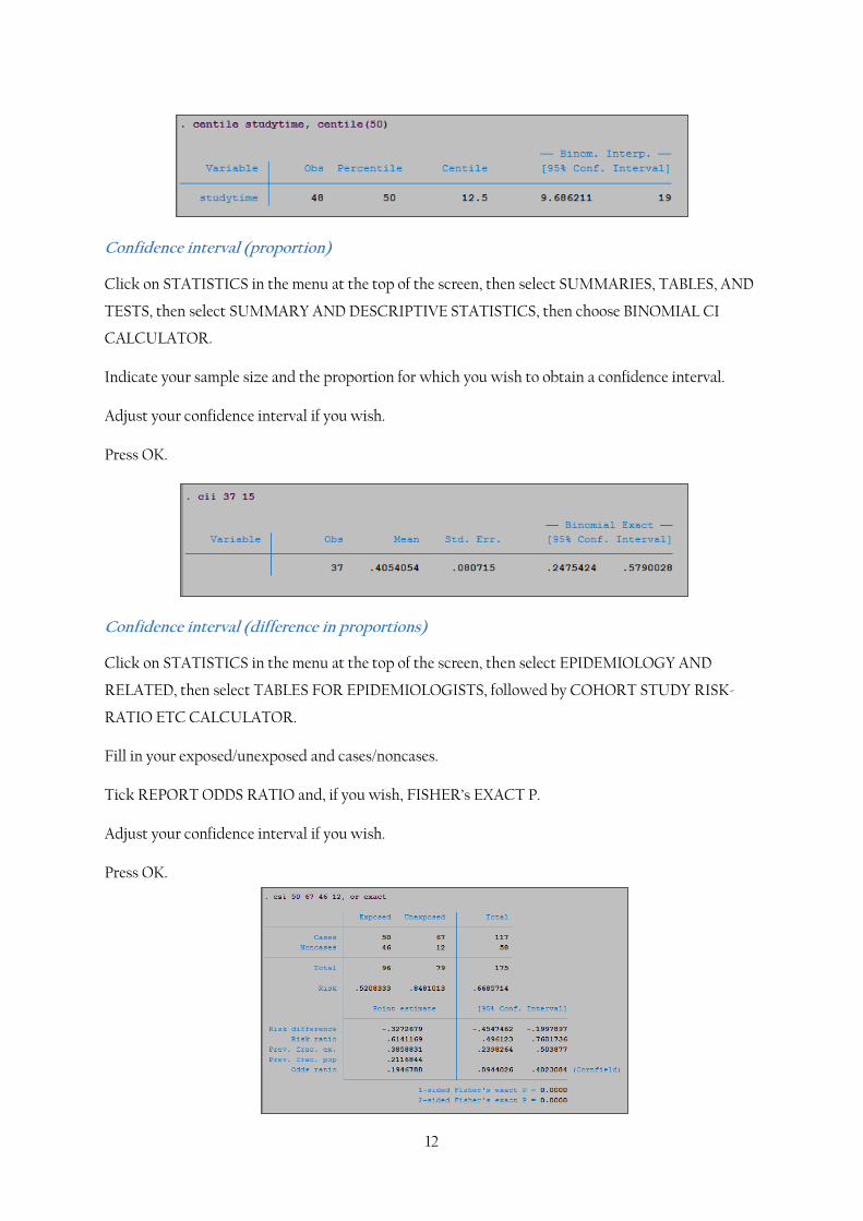
Confidence interval (proportion)


TESTS, then select SUMMARY AND DESCRIPTIVE STATISTICS, then choose BINOMIAL CI

CALCULATOR.

Indicate your sample size and the proportion for which you wish to obtain a confidence interval.

Adjust your confidence interval if you wish.

Press OK.

Confidence interval (difference in proportions)

Click on STATISTICS in the menu at the top of the screen, then select EPIDEMIOLOGY AND

RELATED, then select TABLES FOR EPIDEMIOLOGISTS, followed by COHORT STUDY RISK-

RATIO ETC CALCULATOR.

Fill in your exposed/unexposed and cases/noncases.

Tick REPORT ODDS RATIO and, if you wish, FISHER’s EXACT P.


Press OK.

13

T-tests

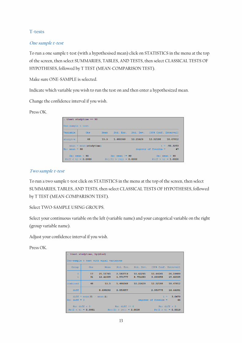
One sample t-test

To run a one sample t-test (with a hypothesised mean) click on STATISTICS in the menu at the top

of the screen, then select SUMMARIES, TABLES, AND TESTS, then select CLASSICAL TESTS OF

HYPOTHESES, followed by T TEST (MEAN-COMPARISON TEST).

Make sure ONE-SAMPLE is selected.

Indicate which variable you wish to run the test on and then enter a hypothesized mean.

Change the confidence interval if you wish.

Press OK.

Two sample t-test

To run a two sample t-test click on STATISTICS in the menu at the top of the screen, then select

SUMMARIES, TABLES, AND TESTS, then select CLASSICAL TESTS OF HYPOTHESES, followed

by T TEST (MEAN-COMPARISON TEST).

Select TWO-SAMPLE USING GROUPS.

Select your continuous variable on the left (variable name) and your categorical variable on the right

(group variable name).


Press OK.

14

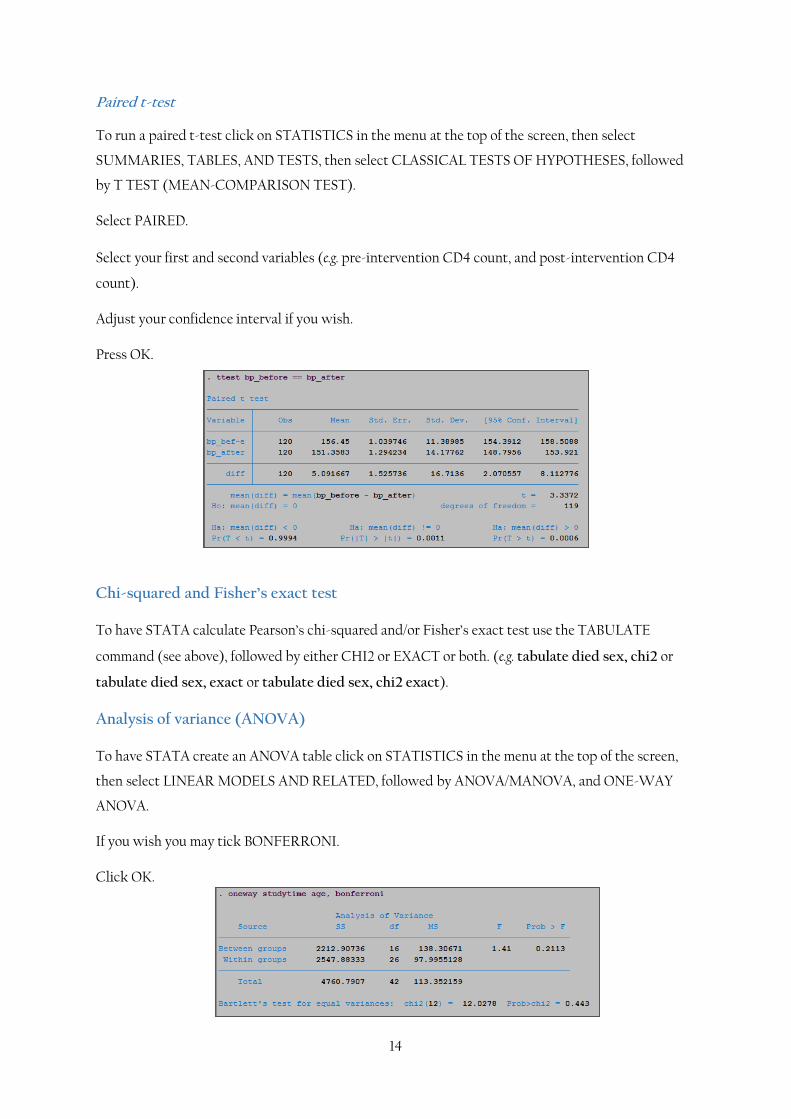
Paired t-test

To run a paired t-test click on STATISTICS in the menu at the top of the screen, then select

SUMMARIES, TABLES, AND TESTS, then select CLASSICAL TESTS OF HYPOTHESES, followed

by T TEST (MEAN-COMPARISON TEST).

Select PAIRED.

Select your first and second variables (e.g. pre-intervention CD4 count, and post-intervention CD4

count).


Press OK.

Chi-squared and Fisher’s exact test

To have STATA calculate Pearson’s chi-squared and/or Fisher’s exact test use the TABULATE

command (see above), followed by either CHI2 or EXACT or both. (e.g. tabulate died sex, chi2 or

tabulate died sex, exact or tabulate died sex, chi2 exact).

Analysis of variance (ANOVA)

To have STATA create an ANOVA table click on STATISTICS in the menu at the top of the screen,

then select LINEAR MODELS AND RELATED, followed by ANOVA/MANOVA, and ONE-WAY

ANOVA.

If you wish you may tick BONFERRONI.

Click OK.

15

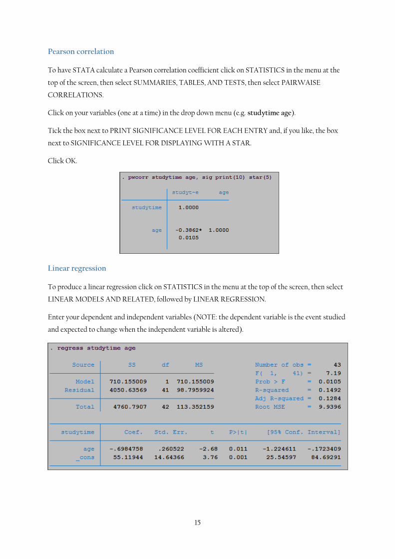
Pearson correlation

To have STATA calculate a Pearson correlation coefficient click on STATISTICS in the menu at the

top of the screen, then select SUMMARIES, TABLES, AND TESTS, then select PAIRWAISE

CORRELATIONS.

Click on your variables (one at a time) in the drop down menu (e.g. studytime age).

Tick the box next to PRINT SIGNIFICANCE LEVEL FOR EACH ENTRY and, if you like, the box

next to SIGNIFICANCE LEVEL FOR DISPLAYING WITH A STAR.

Click OK.

Linear regression

To produce a linear regression click on STATISTICS in the menu at the top of the screen, then select

LINEAR MODELS AND RELATED, followed by LINEAR REGRESSION.

Enter your dependent and independent variables (NOTE: the dependent variable is the event studied

and expected to change when the independent variable is altered).

16

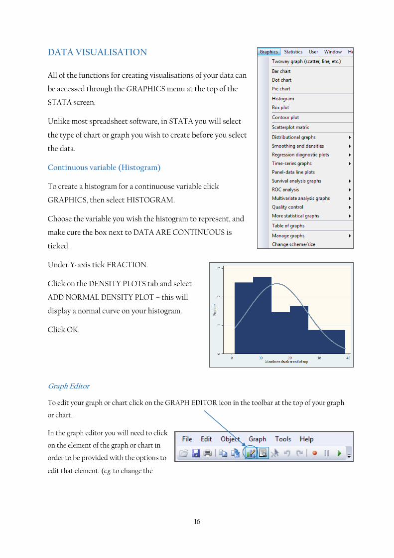
DATA VISUALISATION

All of the functions for creating visualisations of your data can

be accessed through the GRAPHICS menu at the top of the

STATA screen.

Unlike most spreadsheet software, in STATA you will select

the type of chart or graph you wish to create before you select

the data.

Continuous variable (Histogram)

To create a histogram for a continuouse variable click

GRAPHICS, then select HISTOGRAM.

Choose the variable you wish the histogram to represent, and

make cure the box next to DATA ARE CONTINUOUS is

ticked.

Under Y-axis tick FRACTION.

Click on the DENSITY PLOTS tab and select

ADD NORMAL DENSITY PLOT – this will

display a normal curve on your histogram.

Click OK.

Graph Editor

To edit your graph or chart click on the GRAPH EDITOR icon in the toolbar at the top of your graph

or chart.

In the graph editor you will need to click

on the element of the graph or chart in

order to be provided with the options to

edit that element. (e.g. to change the

17

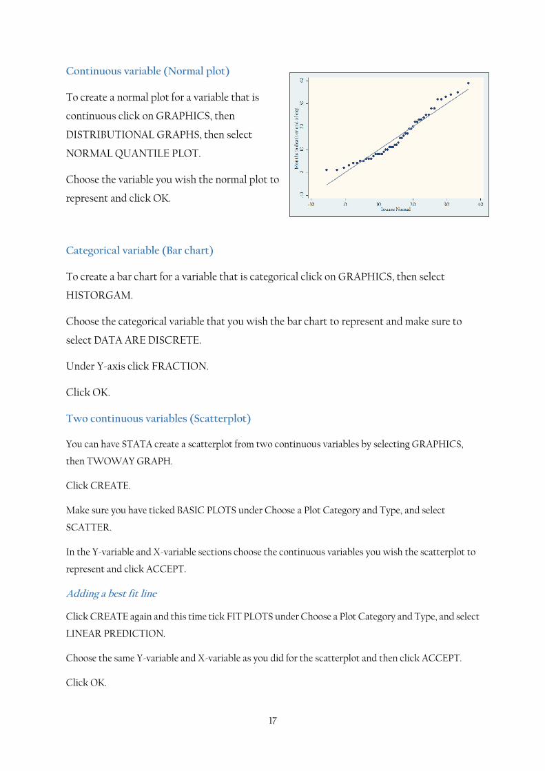
Continuous variable (Normal plot)

To create a normal plot for a variable that is

continuous click on GRAPHICS, then

DISTRIBUTIONAL GRAPHS, then select

NORMAL QUANTILE PLOT.

Choose the variable you wish the normal plot to

represent and click OK.

Categorical variable (Bar chart)

To create a bar chart for a variable that is categorical click on GRAPHICS, then select

HISTORGAM.

Choose the categorical variable that you wish the bar chart to represent and make sure to

select DATA ARE DISCRETE.

Under Y-axis click FRACTION.

Click OK.

Two continuous variables (Scatterplot)

You can have STATA create a scatterplot from two continuous variables by selecting GRAPHICS,

then TWOWAY GRAPH.

Click CREATE.

Make sure you have ticked BASIC PLOTS under Choose a Plot Category and Type, and select

SCATTER.

In the Y-variable and X-variable sections choose the continuous variables you wish the scatterplot to

represent and click ACCEPT.

Adding a best fit line

Click CREATE again and this time tick FIT PLOTS under Choose a Plot Category and Type, and select

LINEAR PREDICTION.

Choose the same Y-variable and X-variable as you did for the scatterplot and then click ACCEPT.

Click OK.

18

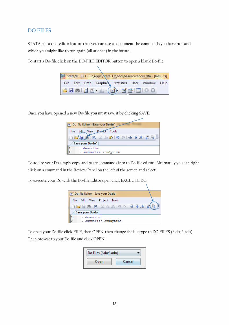
DO FILES

STATA has a text editor feature that you can use to document the commands you have run, and

which you might like to run again (all at once) in the future.

To start a Do-file click on the DO-FILE EDITOR button to open a blank Do-file.

Once you have opened a new Do-file you must save it by clicking SAVE.

To add to your Do simply copy and paste commands into to Do-file editor. Alternately you can right

click on a command in the Review Panel on the left of the screen and select

To execute your Do with the Do-file Editor open click EXCEUTE DO.

To open your Do-file click FILE, then OPEN, then change the file type to DO FILES (*.do; *.ado).

Then browse to your Do-file and click OPEN.

19

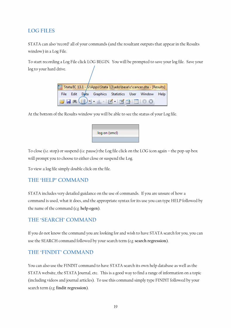
LOG FILES

STATA can also ‘record’ all of your commands (and the resultant outputs that appear in the Results

window) in a Log File.

To start recording a Log File click LOG BEGIN. You will be prompted to save your log file. Save your

log to your hard drive.

At the bottom of the Results window you will be able to see the status of your Log file.

To close (i.e. stop) or suspend (i.e. pause) the Log file click on the LOG icon again – the pop-up box

will prompt you to choose to either close or suspend the Log.

To view a log file simply double click on the file.

THE ‘HELP’ COMMAND

STATA includes very detailed guidance on the use of commands. If you are unsure of how a

command is used, what it does, and the appropriate syntax for its use you can type HELP followed by

the name of the command (e.g. help egen).

THE ‘SEARCH’ COMMAND

If you do not know the command you are looking for and wish to have STATA search for you, you can

use the SEARCH command followed by your search term (e.g. search regression).

THE ‘FINDIT’ COMMAND

You can also use the FINDIT command to have STATA search its own help database as well as the

STATA website, the STATA Journal, etc. This is a good way to find a range of information on a topic

(including videos and journal articles). To use this command simply type FINDIT followed by your

search term (e.g. findit regression).

STATA 13 - London School of Hygiene & Tropical Medicine · 1 INTRODUCTION Versions of STATA STATA offers several different versions of their software. Each has different capabilities

Documents