Volume 4, Issue 5 AUG 2015 IJRAET STAR CONFIGURATION FOR H-BRIDGE INVERTER FED STATCOM S. LAKSHMAN 1 , KANAVENI RAJITHA 2 1 PG Scholor , Brilliant Institute Of Engineering And Technology, Hyderabad, Telangana, India. 2 Asst Professor, Brilliant Institute Of Engineering And Technology, Hyderabad, Telangana, India. Abstract- This paper imposes a multilevel H- bridge converter with star configuration based on Transformerless static synchronous compensator (STATCOM) system. This proposed control methods devote themselves not only to the current loop control but also to the dc capacitor voltage control. The passivity-based controller (PBC) theory is used in this cascaded structure STATCOM for the first time. By adopting a proportional resonant controller an overall voltage control is realized same as the DC capacitor voltage control and an active disturbance rejection controller will provide clustered balancing control. In a field programmable gate array, individual balancing control is achieved by vertically shifting modulation wave. 10KV, 2MVA rated two actual H-bridge cascaded STATCOMs are constructed and a series of verification are executed in simulink MATLAB simulations. Two actual H-bridge cascaded STATCOMs rated at 10 kV 2 MVA are constructed and a series of verification tests are executed. The dc capacitor voltage can be maintained at the given value effectively with fuzzy logic controller . Index Terms— Active disturbances rejection controller (ADRC), H-bridge cascaded, passivity- based control (PBC), proportional resonant (PR) controller, shifting modulation wave, static synchronous compensator (STATCOM). INTRODUCTION Flexible ac transmission systems (FACTS) are being increasingly used in power system to enhance the system utilization, power transfer capacity as well as the power quality of ac system interconnections [1], [2]. As a typical shunt FACTS device, static synchronous compensator (STATCOM) is utilized at the point of common connection (PCC) to absorb or inject the required reactive power, through which the voltage quality of PCC is improved [3]. In recent years, many topologies have been applied to the STATCOM. Among these different types of topology, H-bridge cascaded STATCOM has been widely accepted in high-power applications for the following advantages: quick response speed, small volume, high efficiency, minimal interaction with the supply grid and its individual phase control ability [4]–[7]. Compared with a diode-clamped converter or flying capacitor converter, H-bridge cascaded STATCOM can obtain a high number of levels more easily and can be connected to the grid directly without the bulky transformer. This enables us to reduce cost and improve performance of H-bridge cascaded STATCOM [8].There are two technical challenges which exist in H-bridge cascaded STATCOM to date. First, the control method for the

Welcome message from author
This document is posted to help you gain knowledge. Please leave a comment to let me know what you think about it! Share it to your friends and learn new things together.
Transcript

Volume 4, Issue 5 AUG 2015
IJRAET
STAR CONFIGURATION FOR H-BRIDGE INVERTER FED STATCOM
S. LAKSHMAN1, KANAVENI RAJITHA2
1PG Scholor , Brilliant Institute Of Engineering And Technology, Hyderabad, Telangana, India. 2Asst Professor, Brilliant Institute Of Engineering And Technology, Hyderabad, Telangana, India.
Abstract- This paper imposes a multilevel H-
bridge converter with star configuration based on
Transformerless static synchronous compensator
(STATCOM) system. This proposed control methods
devote themselves not only to the current loop control
but also to the dc capacitor voltage control. The
passivity-based controller (PBC) theory is used in
this cascaded structure STATCOM for the first time.
By adopting a proportional resonant controller an
overall voltage control is realized same as the DC
capacitor voltage control and an active disturbance
rejection controller will provide clustered balancing
control. In a field programmable gate array,
individual balancing control is achieved by vertically
shifting modulation wave. 10KV, 2MVA rated two
actual H-bridge cascaded STATCOMs are
constructed and a series of verification are executed
in simulink MATLAB simulations. Two actual H-bridge
cascaded STATCOMs rated at 10 kV 2 MVA are
constructed and a series of verification tests are executed.
The dc capacitor voltage can be maintained at the given
value effectively with fuzzy logic controller .
Index Terms— Active disturbances rejection
controller (ADRC), H-bridge cascaded, passivity-
based control (PBC), proportional resonant (PR)
controller, shifting modulation wave, static
synchronous compensator (STATCOM).
INTRODUCTION
Flexible ac transmission systems (FACTS)
are being increasingly used in power system to
enhance the system utilization, power transfer
capacity as well as the power quality of ac system
interconnections [1], [2]. As a typical shunt FACTS
device, static synchronous compensator (STATCOM)
is utilized at the point of common connection (PCC)
to absorb or inject the required reactive power,
through which the voltage quality of PCC is
improved [3]. In recent years, many topologies have
been applied to the STATCOM. Among these
different types of topology, H-bridge cascaded
STATCOM has been widely accepted in high-power
applications for the following advantages: quick
response speed, small volume, high efficiency,
minimal interaction with the supply grid and its
individual phase control ability [4]–[7]. Compared
with a diode-clamped converter or
flying capacitor converter, H-bridge cascaded
STATCOM can obtain a high number of levels more
easily and can be connected to the grid directly
without the bulky transformer. This enables us to
reduce cost and improve performance of H-bridge
cascaded STATCOM [8].There are two technical
challenges which exist in H-bridge cascaded
STATCOM to date. First, the control method for the
Gurmeet
Typewritten Text
Gurmeet
Typewritten Text
184

Volume 4, Issue 5 AUG 2015
IJRAET
current loop is an important factor influencing the
compensation performance. However, many nonideal
factors, such as the limited bandwidth of the output
current loop, the time delay induced by the signal
detecting circuit, and the reference command current
generation process, will deteriorate the compensation
effect. Second, H-bridge cascaded STATCOM is a
complicated system with many H-bridge cells in each
phase, so the dc capacitor voltage imbalance issue
which caused by different active power losses among
the cells, different switching patterns for different
cells, parameter variations of active and passive
components inside cells will influence the reliability
of the system and even lead to the collapse of the
system. Hence, lots of researches have focused on
seeking the solutions to these problems.
In terms of current loop control, the majority
of approaches involve the traditional linear control
method, in which the nonlinear equations of the
STATCOM model are linearized with a specific
equilibrium. The most widely used linear control
schemes are PI controllers [9], [10]. In [9], to
regulate reactive power, only a simple PI controller is
carried out. In [10], through a decoupled control
strategy, the PI controller is employed in a
synchronous d–q frame. However, it is hard to find
the suitable parameters for designing the PI controller
and the performance of the PI controller might
degrade with the external disturbance. Thus, a
number of intelligent methods have been proposed to
adapt the PI controller gains such as particle swarm
optimization [11], neural networks [12], and artificial
immunity [13]. In literature [14], [15], adaptive
control and linear robust control have been reported
for their anti-external disturbance ability. In literature
[16], [17], a popular dead-beat current controller is
used. This control method has the high bandwidth
and the fast reference current tracking speed. The
steady-state performance of H-bridge cascaded
STATCOM is improved, but the dynamic
performance is not improved. In [18], a dc injection
elimination method called IDCF is proposed to build
an extra feedback loop for the dc component of the
output current. It can improve the output current
qulity of STATCOM. However, the circuit
configuration of the cascaded STATCOM is the delta
configuration, but not the star configuration.
Moreover, an adaptive theory-based improved linear
sinusoidal tracer control method is proposed in [19]
and a leaky least mean square-based control method
is proposed in [20]. But these methods are not for
STATCOM with the cascaded structure. By using the
traditional linear control method, the controller is
characterized by its simple control structure and
parameter design convenience, but poor dynamic
control stability.
Other control approaches apply nonlinear
control which can directly compensate for the system
nonlinearities without requiring a linear
approximation. In [21], an input–output feedback
linearization controller is designed. By adding a
damping term, the oscillation amplitude of the
internal dynamics can be effectively decreased.
However, the stability cannot be guaranteed [22].
Then, many new modified damping controllers are
designed to enhance the stability and performance of
the internal dynamics [23]–[26]. However, the
implementation of these controllers is very complex.
To enhance robustness and simplify the controller
design, a passivity-based controller (PBC) based on
error dynamics is proposed for STATCOM [27]–
[30]. Furthermore, the exponential stability of system
Gurmeet
Typewritten Text
185
Volume 4, Issue 5 AUG 2015
IJRAET
equilibrium point is guaranteed. Nevertheless, these
methods are not designed on the basis of STATCOM
with the H-bridge cascaded structure and there are no
experimental verifications in these literatures.
In terms of dc capacitor voltage balancing
control, there are three pivotal issues: overall voltage
control, clustered balancing control, and individual
balancing control. In literature [31], under the
asumption of all dc capacitors being equally charged
and balanced, they can only eliminate the imbalances
caused by the inconsistent drive pulses without
detecting all dc capacitor voltages. In [32]–[34],
additional hardware circuits are required in the
methods based on ac bus energy exchange and dc bus
energy exchange, which will increase the cost and the
complexity of the system. In [35], a method based on
zero-sequence voltage injection is proposed and it
will increase the dc capacitor voltage endurance
capacity. On the contrary, the method using negative-
sequence current in [36] does not need the wide
margin of dc capacitor voltage, but the function of
STATCOM is limited. In [8], the active power of the
individual phase cluster is controlled independently,
while the circuit condition is considered to be limited
in practical use. In [37] and [38], a cosine component
of the system voltage is superposed to the clustered
output voltage, but it is easy to be affected by an
inaccurate phase-locked loop (PLL). In [39], the
active voltage vector superposition method is
proposed. However, the simulated and experimental
results do not show the differences in control area
and voltage ripple. The selective harmonic
elimination modulation method is used in [40] and
[41], in which dc voltage balancing control and low-
frequency modulation are achieved. Compared with
the method in [40] and [41], a method changing the
phase-shift angle for dc voltage balancing control is
proposed in [42] and [43], through which the
desirable effect can be easily achieved, whereas it is
limited by the capacity of STATCOM. In [44], the dc
voltage and reactive power are controlled. However,
it cannot be widely used due to fact that many non-
ideal factors are neglected. In [45] and [46], the
proposed method assumes that all cells are distributed
with equal reactive power and it uses the cosine value
of the current phase angle. It could lead to system
instability, when using the zero-crossing point of the
cosine value. In [47] and [48], the results of
experiments are obtained in the downscaled
laboratory system. Thus, they are not very persuasive
in this condition.
In this paper, a new nonlinear control
method based on PBC theory which can guarantee
Lyapunov function dynamic stability is proposed to
control the current loop. It performs satisfactorily to
improve the steady and dynamic response. For dc
capacitor voltage balancing control, by designing a
proportional resonant (PR) controller for overall
voltage control, the control effect is improved,
compared with the traditional PI controller. Active
disturbances rejection controller (ADRC) is first
proposed by Han in his pioneer work [49], and
widely employed in many engineering practices
[50]–[53]; furthermore, it finds its new application in
H-bridge cascaded STATCOM for clustered
balancing control. It realizes the excellent dynamic
compensation for the outside disturbance. By shifting
the modulation wave vertically for individual
balancing control, it is much easier to be realized in
field-programmable gate array (FPGA) compared
with existing methods. Two actual H-bridge cascaded
STATCOMs rated at 10 kV 2 MVA are constructed
Gurmeet
Typewritten Text
186
Volume 4, Issue 5 AUG 2015
IJRAET
and a series of verification tests are executed. The
experimental results have verified the viability and
effectiveness of the proposed control methods.
II. CONFIGURATION OF THE 10KV
2MVA STATCOM SYSTEM
Fig. 1 shows the circuit configuration of the
10 kV 2 MVA star-configured STATCOM cascading
12 H-bridge pulse width modulation (PWM)
converters in each phase and it can be expanded
easily according to the requirement. By controlling
the current of STATCOM directly, it can absorb or
provide the required reactive current to achieve the
purpose of dynamic reactive current compensation.
Finally, the power quality of the grid is improved and
the grid offers the active current only. The power
switching devices working in ideal condition is
assumed. 푢 , 푢 , and 푢 are the three-phase
voltage of grid. 푢 , 푢 , and 푢 are the three-phase
voltage of STATCOM. 푖 ,푖 and 푖 , are the three-
phase current of grid. 푖 , 푖 , and 푖 , are the three-
phase current of STATCOM. 푖 ,푖 , and푖 , are the
three-phase current of load. 푈 is the reference
voltage of dc capacitor. C is the dc capacitor. L is the
inductor. 푅 is the starting resistor.
Table I summarizes the circuit parameters. The
cascade number of N=12is assigned to H-bridge
cascaded STATCOM, resulting in 36 H-bridge cells
in total. Every cell is equipped with nine isolated
electrolytic capacitors which the capacitance is
5600μF. The dc side has no external circuit and no
power source except for the dc capacitor and the
voltage sensor. In each cluster, an ac inductor
supports the difference between the sinusoidal
TABLE I
CIRCUIT PARAMETERS OF THE
EXPERIMENTAL RESULTS
Grid voltage 푢 10kV
Rated reactive 푄 2MVA
AC inductor 퐿 10mH
Starting resistor 푅 4푘Ω
DC capacitor Capacitance 퐶 5600휇퐹
DC capacitor reference voltage 푈 800V
Number of H-bridges 푁 12
PWM carrier frequency 푓 1kHz
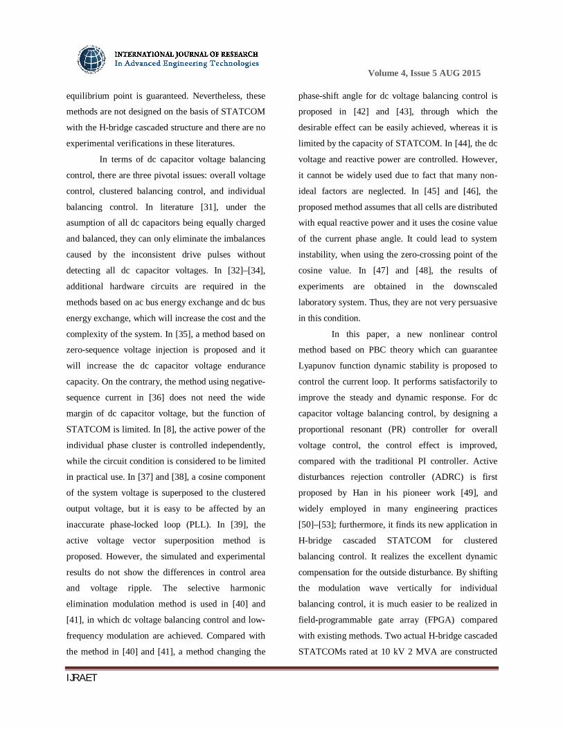
Fig. 2. Digital control system for 10 kV 2 MVA H-
bridge cascaded STATCOM.
frequency of 1 kHz. Then, with a cascade number of
N=12, the ac voltage cascaded results in a 25-level
waveform in line to neutral and a 49-level waveform
in line to line. In each cluster, 12 carrier signals with
Gurmeet
Typewritten Text
187

Volume 4, Issue 5 AUG 2015
IJRAET
the same frequency as 1 kHz are phase shifted by
2π/12 from each other. When a carrier frequency is
as low as 1 kHz, using the method of phase-shifted
uni-polar sinusoidal PWM, it can make an equivalent
carrier frequency as high as 24 kHz. The lower
carrier frequency can also reduce the switching losses
to each cell. As shown in Fig. 2, the main digital
control block diagram of the 10 kV 2 MVA
STATCOM experimental system consists of a digital
signal processor (DSP) (Texas Instruments
TMS320F28335), an FPGA ( Altera CycloneIII
EP3C25), and 36 complex programmable logic
devices (CPLDs) (Altera MAXII EPM570). Most of
the calculations, such as the detection of reactive
current and the computation of reference voltage, are
achieved by DSP. Then, DSP sends the reference
voltages to the FPGA. The FPGA implements the
modulation strategy and generates 36 PWM
switching signals for each cell. CPLD of each cell
receives PWM switching signal from the FPGA and
drives IGBTs.
III. CONTROLALGORITHM
Fig. 3 shows a block diagram of the control
algorithm for H-bridge cascaded STATCOM. The
whole control algorithm mainly consists of four parts,
namely, PBC, overall voltage control, clustered
balancing control, and individual balancing control.
The first three parts are achieved in DSP, while the
last part is achieved in the FPGA.
Fig. 3. Control block diagram for the 10 kV 2 MVA
H-bridge cascaded STATCOM.
A. PBC
Referring to Fig. 1, the following set of voltage and
current equations can be derived:
⎩⎪⎨
⎪⎧퐿 = 푢 − 푢 − R푖
퐿 = 푢 − 푢 − R푖
퐿 = 푢 − 푢 − R푖
---(1)
Where R is the equivalent series resistance of the
inductor. Applying the d–q transformations (1), the
equations in d–q axis are obtained.
퐿푑푖푑푡 = −푅푖 +휔퐿푖 + 푢 − 푢
퐿푑푖푑푡 = −휔퐿푖 − 푅푖 + 푢 − 푢
--------(2)
Where 푈 and 푈 are the d-axis and q-axis
components corresponding to the three-phase
STATCOM cluster voltages푈 , 푈 , and 푈 . 푈 and
푈 are those corresponding to the three-phase grid
voltages 푈 , 푈 , and 푈 . When the grid voltages
are sinusoidal and balanced, 푈 is always 0 because
of 푈 is aligned with the d-axis. Id and Iq are the d-
axis and q-axis components corresponding to the
three-phase STATCOM currents퐼 , 퐼 , and 퐼 .
Gurmeet
Typewritten Text
Gurmeet
Typewritten Text
188
Volume 4, Issue 5 AUG 2015
IJRAET
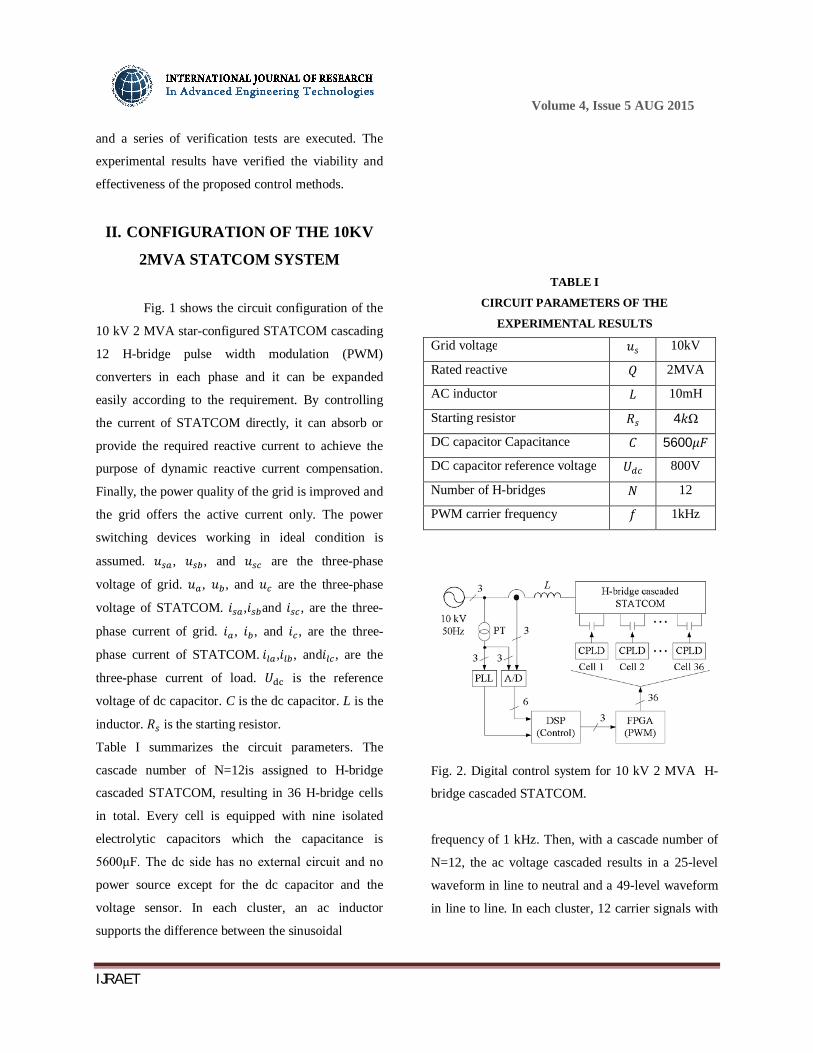
Equation (2) is written as the following form:
퐿 00 퐿
퐼 퐼 + 푅 0
0 푅퐼 퐼 =
푢 −푢푢 −푢
--(3)
To apply the PBC method, (3) is transformed into the
form of the EL system model in this paper. EL
system model is an important part of the nonlinear
PBC theory and an effective modeling technology. It
defines the energy equation by setting the general
variable and harnesses the known theorem that can be
used to analyze the dynamic performance to deduce
the dynamic equations. This can make the system
move along the minimize trajectory of Lagrangian
integral [54]. EL system model could describe the
characteristics of the system which is difficult to be
disposed by linearization control method. This is the
most important reason to use the EL system model
for defining control system of H-bridge cascaded
STATCOM. Referring to [54], along with selecting
퐼 and 퐼 as state variables, it gives the following EL
system model of (3):
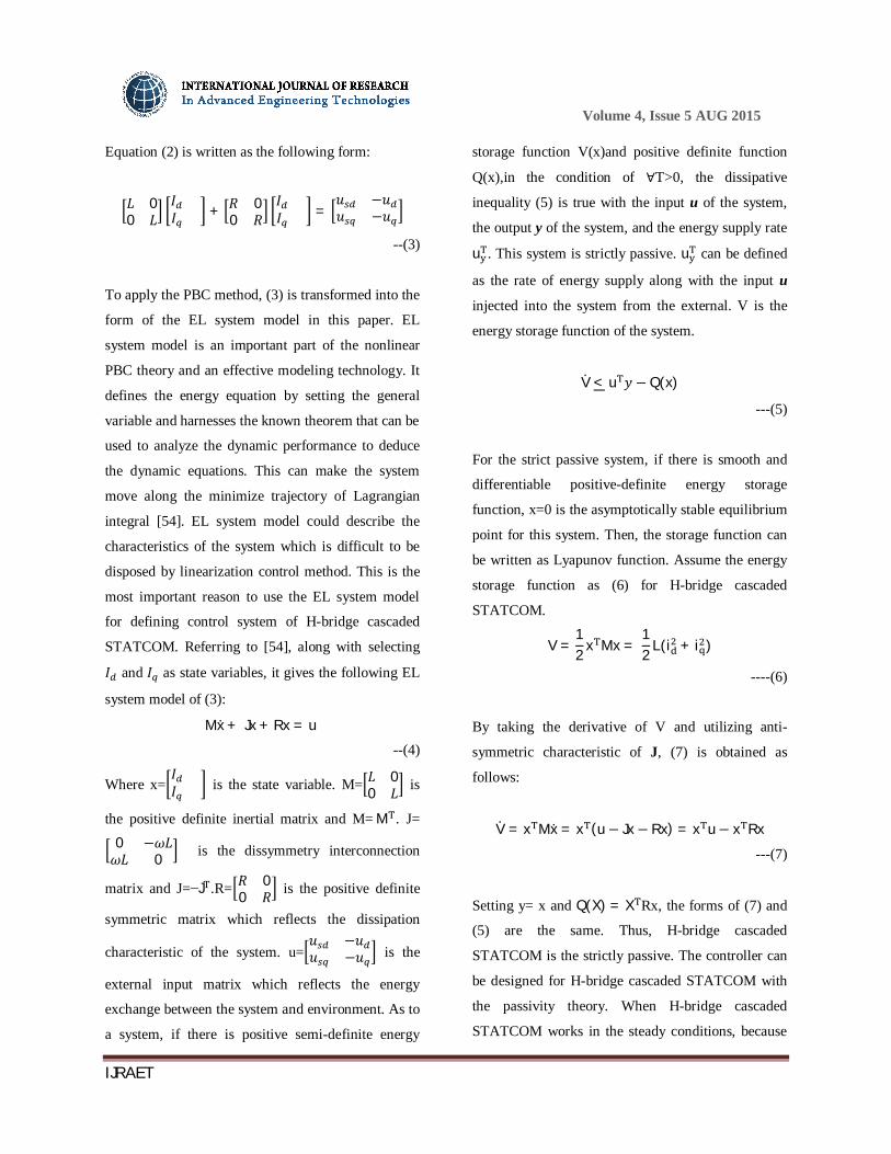
Mx + Jx + Rx = u --(4)
Where x=퐼 퐼 is the state variable. M= 퐿 0
0 퐿 is
the positive definite inertial matrix and M= M . J=
0 −휔퐿휔퐿 0 is the dissymmetry interconnection
matrix and J=−J .R= 푅 00 푅 is the positive definite
symmetric matrix which reflects the dissipation
characteristic of the system. u=푢 −푢푢 −푢 is the
external input matrix which reflects the energy
exchange between the system and environment. As to
a system, if there is positive semi-definite energy
storage function V(x)and positive definite function
Q(x),in the condition of ∀T>0, the dissipative
inequality (5) is true with the input u of the system,
the output y of the system, and the energy supply rate
u . This system is strictly passive. u can be defined
as the rate of energy supply along with the input u
injected into the system from the external. V is the
energy storage function of the system.
V < u 푦 − Q(x)
---(5)
For the strict passive system, if there is smooth and
differentiable positive-definite energy storage
function, x=0 is the asymptotically stable equilibrium
point for this system. Then, the storage function can
be written as Lyapunov function. Assume the energy
storage function as (6) for H-bridge cascaded
STATCOM.
V =12 x Mx =
12 L(i + i )
----(6)
By taking the derivative of V and utilizing anti-
symmetric characteristic of J, (7) is obtained as
follows:
V = x Mx = x (u − Jx − Rx) = x u− x Rx
---(7)
Setting y= x and Q(X) = X Rx, the forms of (7) and
(5) are the same. Thus, H-bridge cascaded
STATCOM is the strictly passive. The controller can
be designed for H-bridge cascaded STATCOM with
the passivity theory. When H-bridge cascaded
STATCOM works in the steady conditions, because
Gurmeet
Typewritten Text
189
Volume 4, Issue 5 AUG 2015
IJRAET
of the switching loss, the equivalent resistance loss
and the loss of the capacitor itself, it will lead to a
decline of the dc capacitor voltage. Thus, it needs to
maintain dc capacitor voltage at the given value
while compensating the reactive current for grid. And
it has three expected stable equilibrium points: U is
the dc capacitor reference voltage. 푖∗ is the reference
current of the d-axis. 푖∗ is the reference current of the
q-axis.
Generally, the dc capacitor voltage of H-bridge
cascaded STATCOM is maintained at the given value
through absorbing the active current from the grid
that can be achieved by controlling the d-axis active
current. This d-axis active current 푖∗ =푖 +푖 (as
shown in Fig. 3) can be added to the d-axis reference
current. The newfound d-axis reference current is
푖∗ = i∗+i∗ . Now, the three expected stable
equilibrium points of the system can be revised two:
푥∗ = 푖∗ and 푥∗ =i∗ . Error system is established as
follows:
x = x− x∗ = [푖 − 푖∗ 푖 − 푖∗]
---(8)
Where 푥∗ is the expected stable equilibrium point of
the system. Substituting (8) into (4), the error
dynamic equation of the system can be obtained as
follows:
M(x + x∗) + J(x + x∗) = u
---(9)
That is
Mx + Jx + Rx = u − (Mx∗ + Jx∗ + Rx∗)
--(10)
To improve the speed of the convergence, from x to
x∗, and make error energy function reach zero, (10) is
injected with damping. It can accelerate energy
dissipation of the system and make the system
converge the expected stable equilibrium point. The
injected damping dissipation term as follows:
푅 x = (푅 + 푅 )x
-----(11)
Where 푅 is the damping matrix of the system. Ra
= 푅 00 푅 is the injected positive definite
damping matrix and 푅 > 0, 푅 > 0.
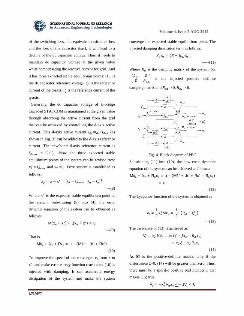
Fig. 4. Block diagram of PBC
Substituting (11) into (10), the new error dynamic
equation of the system can be achieved as follows:
Mx + Jx + R x = u − (Mx∗ + Jx∗ + Rx∗ − R x )
= x
-----(12)
The Lyapunov function of the system is obtained as
V =12 x Mx =
12 L 푖 + 푖
---(13)
The derivative of (13) is achieved as
V = 푥 푀푥 = 푥 (휉 − 퐽푥 − 푅 푥 )
= 푥 휉 − 푥 푅 푥
----(14)
As M is the positive-definite matrix, only if the
disturbance ξ=0, (14) will be greater than zero. Thus,
there must be a specific positive real number λ that
makes (15) true
V = −x R 푥 <− 휆V < 0
Gurmeet
Typewritten Text
190
Volume 4, Issue 5 AUG 2015
IJRAET
----(15)
According to Lyapunov stability theorem, the system
is exponential asymptotic stability. For making ξ=0,
the system needs to satisfy the condition as
Mx∗ + Jx∗ + Rx∗ − R x
-----(16)
Based on (16), the passivity-based controller for H-
bridge cascaded STATCOM can be obtained as
푢 = −퐿푑푖∗
푑푡+ 휔퐿푖∗ − 푅푖∗ + 푅 (푖 − 푖∗ ) + 푢
푢 = −퐿푑푖∗
푑푡+ 휔퐿푖∗ − 푅푖∗ + 푅 푖 − 푖∗ + 푢 .
---(18)
Fig. 4 shows a block diagram of the PBC and the
three-phase command voltages u∗ , u∗ , and u∗ can be
obtained by applying the inverse d–q transformation
to u and u .
B. OVERALL VOLTAGE CONTROL
As the first-level control of the dc capacitor voltage
balancing, the aim of the overall voltage control is to
keep the dc mean voltage of all converter cells
equalling to the dc capacitor reference voltage. The
common approach is to adopt the conventional PI
controller which is simple to implement. However,
the output voltage and current of H-bridge cascaded
STATCOM are the power frequency sinusoidal
variables and the output power is the double power
frequency sinusoidal variable, it will make the dc
capacitor also has the double power frequency ripple
voltage.
So, the reference current which is obtained in the
process of the overall voltage control is not a
standard dc variable and it also has the double power
frequency alternating component and it will reduce
the quality of STATCOM output current. In general,
when using PI controller, in order to ensure the
stability and the dynamic performance of system, the
bandwidth of voltage loop control is set to be 200–
500 Hz and it is difficult to restrain the negative
effect on the quality of STATCOM output current
which is caused by the 100 Hz ripple voltage.
Moreover, because of static error of PI controller, it
will affect not only the first level control but also the
second and the third one. Especially, during the
startup process of STATCOM, it will make the
voltage reach the target value with a much larger
overshoot. To resolve the problem, this paper adopts
the PR controller for the overall voltage control. The
gain of the PR controller is infinite at the
fundamental frequency and very small at the other
frequency. Consequently, the system can achieve the
zero steady-state error at the fundamental frequency.
By setting the cutoff frequency and the resonant
frequency of the PR controller appropriately, it can
reduce the part of ripple voltage in total error,
decrease the reference current distortion which is
caused by ripple voltage, and improve the quality of
STATCOM output current. Moreover, the dynamic
performance and the dynamic response speed of the
system also can be improved. In particular, during the
startup process of STATCOM, the much larger dc
voltage overshoot can be restrained effectively. The
PR controller is composed of a proportional regulator
and a resonant regulator. Its transfer function can be
expressed as
퐺 (푠) = 푘 +2푘 휔 푠
푠 + 2휔 +휔
----(18)
Where 푘 is the proportional gain coefficient. 푘 is
the integral gain coefficient. 휔 is the cutoff
frequency. ω is the resonant frequency.푘 influences
Gurmeet
Typewritten Text
191
Volume 4, Issue 5 AUG 2015
IJRAET
the gain of the controller but the bandwidth. With 푘
increasing, the amplitude at the resonant frequency is
also increased and it plays a role in the elimination
of the steady-state error. ω influences the gain of the
controller and the bandwidth. With 휔 increasing, the
gain and the bandwidth of the controller are both
increased.
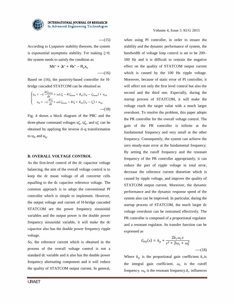
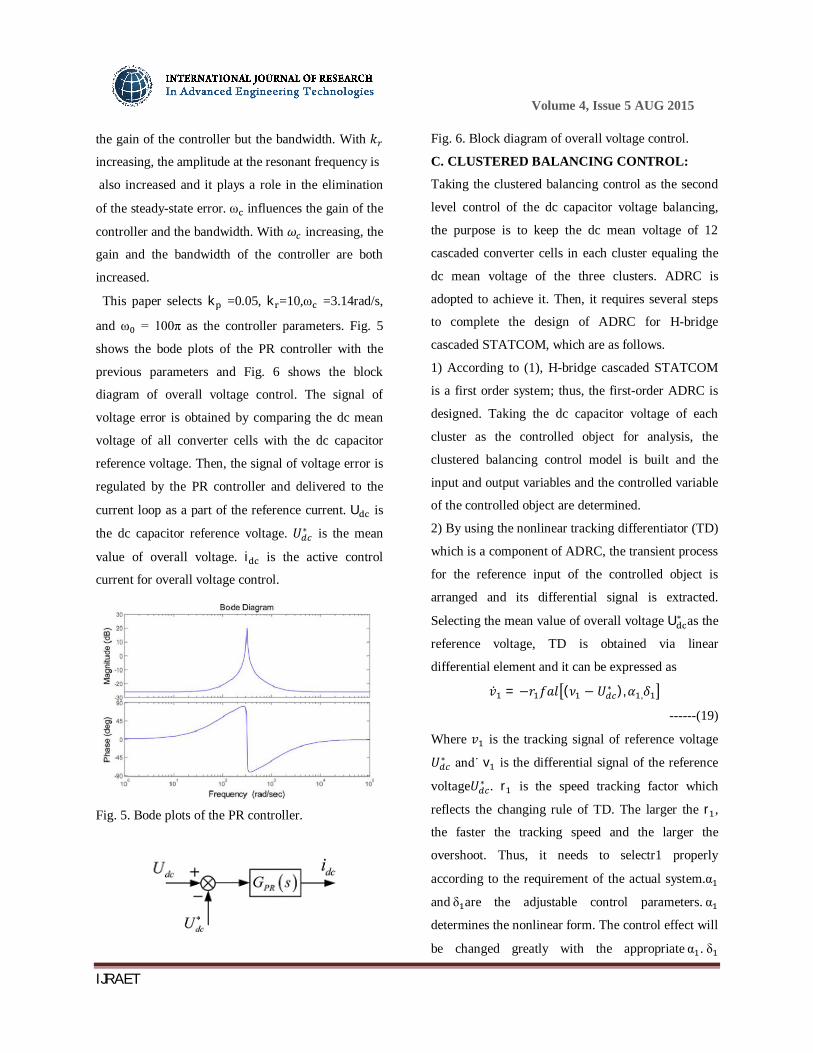
This paper selects k =0.05, k =10,ω =3.14rad/s,
and ω = 100π as the controller parameters. Fig. 5
shows the bode plots of the PR controller with the
previous parameters and Fig. 6 shows the block
diagram of overall voltage control. The signal of
voltage error is obtained by comparing the dc mean
voltage of all converter cells with the dc capacitor
reference voltage. Then, the signal of voltage error is
regulated by the PR controller and delivered to the
current loop as a part of the reference current. U is
the dc capacitor reference voltage. 푈∗ is the mean
value of overall voltage. i is the active control
current for overall voltage control.
Fig. 5. Bode plots of the PR controller.
Fig. 6. Block diagram of overall voltage control.
C. CLUSTERED BALANCING CONTROL:
Taking the clustered balancing control as the second
level control of the dc capacitor voltage balancing,
the purpose is to keep the dc mean voltage of 12
cascaded converter cells in each cluster equaling the
dc mean voltage of the three clusters. ADRC is
adopted to achieve it. Then, it requires several steps
to complete the design of ADRC for H-bridge
cascaded STATCOM, which are as follows.
1) According to (1), H-bridge cascaded STATCOM
is a first order system; thus, the first-order ADRC is
designed. Taking the dc capacitor voltage of each
cluster as the controlled object for analysis, the
clustered balancing control model is built and the
input and output variables and the controlled variable
of the controlled object are determined.
2) By using the nonlinear tracking differentiator (TD)
which is a component of ADRC, the transient process
for the reference input of the controlled object is
arranged and its differential signal is extracted.
Selecting the mean value of overall voltage U∗ as the
reference voltage, TD is obtained via linear
differential element and it can be expressed as
푣 = −푟 푓푎푙 (휈 − 푈∗ ),훼 ,훿
------(19)
Where 푣 is the tracking signal of reference voltage
푈∗ and˙ v is the differential signal of the reference
voltage푈∗ . r is the speed tracking factor which
reflects the changing rule of TD. The larger the r ,
the faster the tracking speed and the larger the
overshoot. Thus, it needs to selectr1 properly
according to the requirement of the actual system.α
and δ are the adjustable control parameters. α
determines the nonlinear form. The control effect will
be changed greatly with the appropriate α . δ
Gurmeet
Typewritten Text
Gurmeet
Typewritten Text
192
Volume 4, Issue 5 AUG 2015
IJRAET
determines the size of the falfunction linear range. 3).
With the extended state observer (ESO) in ADRC,
the uncertainties and the disturbances which lead to
the unbalancing of the clustered dc capacitor voltages
are observed and estimated dynamically. The second-
order ESO designed for the dc capacitor voltage of
STATCOM could be written as
휉 = 푧 − 푈
푧 = 푧 − 푟 푓푎푙(휉,훼 ,훿 ) + 푏∆푖푧 = −푟 푓푎푙(휉,훼 ,훿 )
------(21)
Where the falfunction fal(ξ, α, δ) is defined as.
푈 (k=a, b, c)is the real-time detected value of the
dc mean voltage of 12 cascaded converter cells in
each cluster in current cyclical and it is used as
known parameter.z1is the state estimation signal of
the dc capacitor voltage. ξ is the control deviation of
the system.Z is the internal and the external
disturbance estimate signals of the controlled object.
Δi is the control variable. b is the feedback
coefficient of Δi (k=a, b, c). r , r , α , andδ are
the adjustable control parameters. r has an effect on
the delay of Z . The larger the r , the smaller the
delay. But, the larger r will lead to system
oscillation. With r increasing slightly, the system
oscillation could be damped. However, it will result
in system divergence. Consequently, the adjustment
ofr and r requires mutual coordination. It can
setr before hand and then improve the control
effect with increasing r gradually.
Actually, there are errors in the detection unit of the
dc capacitor voltage of STATCOM. Thus, control
precision of the dc capacitor voltage can be improved
considerably by using 푍 to estimate the state of the
actual dc capacitor voltage precisely. For the
changing of the system operation parameters in
different applied environments,Z can estimate the
unknown disturbances accurately and optimize the
dynamic response speed of the clustered balancing
control. Whether the unknown disturbances can be
estimated accurately with ESO directly influences the
control effect of ADRC. Therefore, the tuning of
ESO parameters is very critical.
4) Nonlinear state error feedback (NLSEF) unit, a
very important part of ADRC, is used to calculate the
control variable of the active power adjustment for
the clustered balancing control. However, in the
practical application, the selection of NLSEF unit
parameters in common ADRC is very difficult.
Therefore, it is simplified with the linear optimization
method in this paper and the newly obtained NLSEF
unit can be expressed as
휉 = 푧 − 휐푖 = 푟 푓푎푙(휉 ,훼 ,훿 )
Δ푖 = 푖 − 푧 /푏
------(22)
Where falfunction is defined as (21). ξ is the error
value between the tracking signal v and the state
estimation signal z .
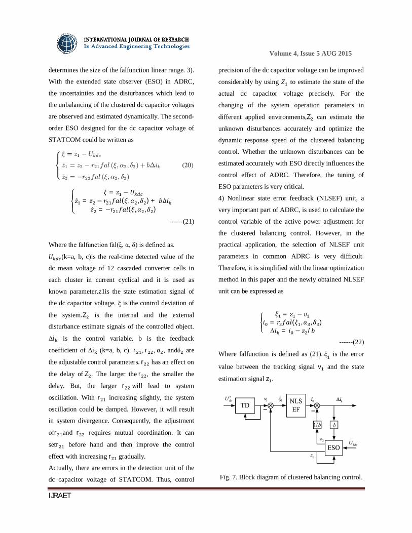
Fig. 7. Block diagram of clustered balancing control.
Gurmeet
Typewritten Text
193
Volume 4, Issue 5 AUG 2015
IJRAET
푖 is the control variable without the disturbance
feedback compensation.bis the feedback coefficient
which has relations with the control variable Δi and
the state variable of the ESO. If the controlled object
existed delay, with a larger b, it would generate a
large error control signal making the response speed
of the output faster and compensation of the internal
and the external disturbances more effective.r ,α ,
and δ are the adjustable control parameters. The
regulating speed can be controlled by appropriately
adjusting r . However, the faster regulating speed
might cause increased overshoot and system
oscillation.
5) Finally, by combining NLSEF unit with the
observed disturbances from ESO, the simplified
ADRC can be achieved and then the clustered
balancing control of H-bridge cascaded STATCOM
can be realized.
Fig. 7 shows a block diagram of the clustered
balancing control with the simplified ADRC. When
ADRC receives the reference voltage U∗ and the
real-time detected value of the dc mean voltage
푈 (k=a, b, c)of 12 cascaded converter cells in each
cluster, it will trace the reference voltage rapidly with
TD and obtain the tracking signalv1by filtering.
Then, by subtracting the tracking signal V from the
state estimation signal of the dc capacitor voltage z ,
the control deviation command ξ of the system
voltage is calculated. ξ is used as the input signal of
NLSEF. Finally, the active adjustment control current
Δi (k=a, b, c) of the clustered balancing control is
achieved by subtracting the disturbance estimate
signals which obtained in ESO from the output result
i of NLSEF.
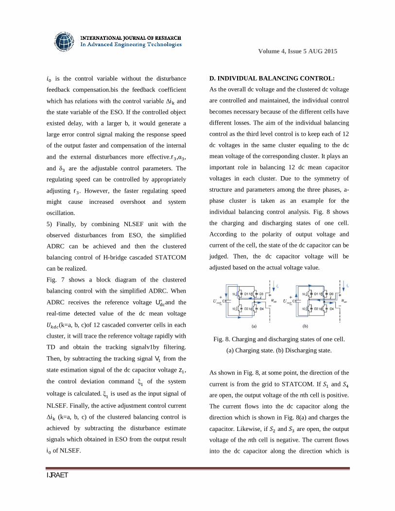
D. INDIVIDUAL BALANCING CONTROL:
As the overall dc voltage and the clustered dc voltage
are controlled and maintained, the individual control
becomes necessary because of the different cells have
different losses. The aim of the individual balancing
control as the third level control is to keep each of 12
dc voltages in the same cluster equaling to the dc
mean voltage of the corresponding cluster. It plays an
important role in balancing 12 dc mean capacitor
voltages in each cluster. Due to the symmetry of
structure and parameters among the three phases, a-
phase cluster is taken as an example for the
individual balancing control analysis. Fig. 8 shows
the charging and discharging states of one cell.
According to the polarity of output voltage and
current of the cell, the state of the dc capacitor can be
judged. Then, the dc capacitor voltage will be
adjusted based on the actual voltage value.
Fig. 8. Charging and discharging states of one cell.
(a) Charging state. (b) Discharging state.
As shown in Fig. 8, at some point, the direction of the
current is from the grid to STATCOM. If 푆 and 푆
are open, the output voltage of the nth cell is positive.
The current flows into the dc capacitor along the
direction which is shown in Fig. 8(a) and charges the
capacitor. Likewise, if 푆 and 푆 are open, the output
voltage of the nth cell is negative. The current flows
into the dc capacitor along the direction which is
Gurmeet
Typewritten Text
194
Volume 4, Issue 5 AUG 2015
IJRAET
shown in Fig. 8(b) and discharges the capacitor.
Obviously, to make the capacitor voltage of each cell
tend to be consistent, the turn-on time of the cell with
the lower voltage should be extended and the turn-on
time of the cell with the higher voltage should be
shortened in charging state. Then, in discharging
state, the process is contrary. The adjustment
principle of the dc capacitor voltage can be
summarized as follows.
1) When(푖 ×U )>0,if U <U , it needs to
increase the duty cycle. If U > U , it needs to
reduce the duty cycle.
2) When(푖 ×U )<0,if U >U , it needs to
increase the duty cycle. If U <U , it needs to
reduce the duty cycle.
푖 is output current of a-phase cluster. U is ac
output voltage of the nth(n=1,2,···,12)cell of a-phase
cluster. U is the dc mean voltage of 12 cascaded
converter cells in a-phase cluster. U is the
capacitor voltage of the nth cell of a-phase cluster.
According to the previous method, the direction and
the magnitude of adjustment of the duty cycle for one
cell can be achieved easily at some point. Fig. 9
shows the adjustment method of the duty cycle by
shifting the modulation wave vertically. Taking the
first half period of the modulation wave as an
example, the value of the modulation wave is greater
than zero and the cell outputs zero level and 1 level.
When the level is zero, the capacitor is not connected
to the main circuit and it is not in the state of the
charging and discharging. To reduce the charging
time for one capacitor, it needs to reduce the action
time of 1 level and it can be realized by reducing the
turn-on time of S and S (as shown in Fig. 8). The
state of the left bridge arm is decided by comparing
the normal modulation wave with the triangular
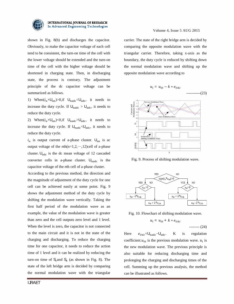
carrier. The state of the right bridge arm is decided by
comparing the opposite modulation wave with the
triangular carrier. Therefore, taking x-axis as the
boundary, the duty cycle is reduced by shifting down
the normal modulation wave and shifting up the
opposite modulation wave according to
푢 = 푢 − 푘 ∗ 푒
-----------(23)
Fig. 9. Process of shifting modulation wave.
Fig. 10. Flowchart of shifting modulation wave.
푢 = 푢 + 푘 ∗ 푒
-------- (24)
Here 푒 =U −U . K is regulation
coefficient.푢 is the previous modulation wave. 푢 is
the new modulation wave. The previous principle is
also suitable for reducing discharging time and
prolonging the charging and discharging times of the
cell. Summing up the previous analysis, the method
can be illustrated as follows.
Gurmeet
Typewritten Text
195

Volume 4, Issue 5 AUG 2015
IJRAET
1) If the requirement is to reduce the duty cycle, it
needs to shift down the normal modulation wave and
shift up the opposite modulation wave.
2) If the requirement is to prolong the duty cycle, it
needs to shift up the normal modulation wave and
shift down the opposite modulation wave.
The value of shifting is decided by 푘 ∗ 푒 and the
flowchart is shown in Fig. 10. The previous method
is the modulation strategy that is based on CPS-
SPWM in this paper and it is very easy to be realized
in the FPGA. But, it is not to say that this method
must be used like this only. In order to regulate the
duty cycle, as long as the pulse signal is achieved by
comparing the modulation wave with the carrier, the
modulation strategy is able to use this method. The
implementation block diagram of the individual
balancing control method is shown in Fig. 11.
Fig. 11. Block diagram of individual balancing
control.
FUZZY LOGIC CONTROLLER
In FLC, basic control action is determined
by a set of linguistic rules. These rules are
determined by the system. Since the numerical
variables are converted into linguistic variables,
mathematical modeling of the system is not required
in FC. The FLC comprises of three parts:
fuzzification, interference engine and defuzzification.
The FC is characterized as i. seven fuzzy sets for
each input and output. ii. Triangular membership
functions for simplicity. iii. Fuzzification using
continuous universe of discourse. iv. Implication
using Mamdani’s, ‘min’ operator. v. Defuzzification
using the height method.
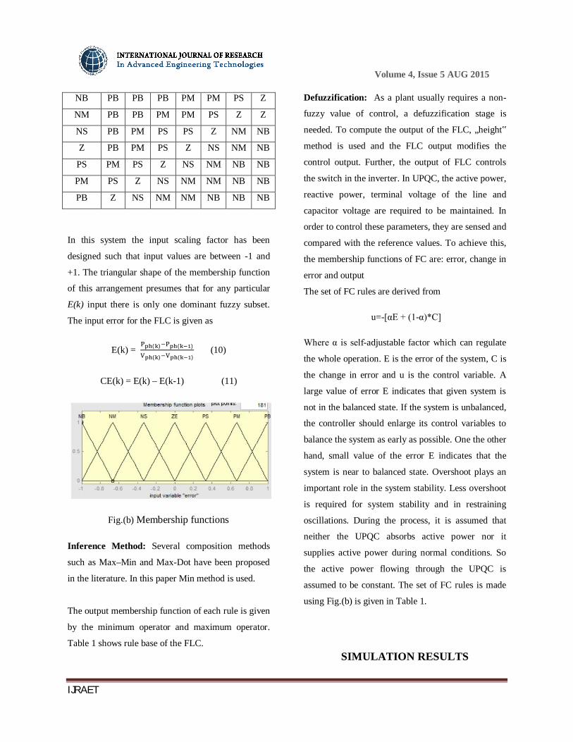
Fuzzification: Membership function values are
assigned to the linguistic variables, using seven fuzzy
subsets: NB (Negative Big), NM (Negative Medium),
NS (Negative Small), ZE (Zero), PS (Positive Small),
PM (Positive Medium), and PB (Positive Big). The
Fig.(a) Fuzzy logic controller
partition of fuzzy subsets and the shape of
membership CE(k) E(k) function adapt the shape up
to appropriate system. The value of input error and
change in error are normalized by an input scaling
factor
Table I Fuzzy Rules
Change
in error
Error
NB NM NS Z PS PM PB
Gurmeet
Typewritten Text
196
Volume 4, Issue 5 AUG 2015
IJRAET
NB PB PB PB PM PM PS Z
NM PB PB PM PM PS Z Z
NS PB PM PS PS Z NM NB
Z PB PM PS Z NS NM NB
PS PM PS Z NS NM NB NB
PM PS Z NS NM NM NB NB
PB Z NS NM NM NB NB NB
In this system the input scaling factor has been
designed such that input values are between -1 and
+1. The triangular shape of the membership function
of this arrangement presumes that for any particular
E(k) input there is only one dominant fuzzy subset.
The input error for the FLC is given as
E(k) = ( ) ( )
( ) ( ) (10)
CE(k) = E(k) – E(k-1) (11)
Fig.(b) Membership functions
Inference Method: Several composition methods
such as Max–Min and Max-Dot have been proposed
in the literature. In this paper Min method is used.
The output membership function of each rule is given
by the minimum operator and maximum operator.
Table 1 shows rule base of the FLC.
Defuzzification: As a plant usually requires a non-
fuzzy value of control, a defuzzification stage is
needed. To compute the output of the FLC, „height‟
method is used and the FLC output modifies the
control output. Further, the output of FLC controls
the switch in the inverter. In UPQC, the active power,
reactive power, terminal voltage of the line and
capacitor voltage are required to be maintained. In
order to control these parameters, they are sensed and
compared with the reference values. To achieve this,
the membership functions of FC are: error, change in
error and output
The set of FC rules are derived from
u=-[αE + (1-α)*C]
Where α is self-adjustable factor which can regulate
the whole operation. E is the error of the system, C is
the change in error and u is the control variable. A
large value of error E indicates that given system is
not in the balanced state. If the system is unbalanced,
the controller should enlarge its control variables to
balance the system as early as possible. One the other
hand, small value of the error E indicates that the
system is near to balanced state. Overshoot plays an
important role in the system stability. Less overshoot
is required for system stability and in restraining
oscillations. During the process, it is assumed that
neither the UPQC absorbs active power nor it
supplies active power during normal conditions. So
the active power flowing through the UPQC is
assumed to be constant. The set of FC rules is made
using Fig.(b) is given in Table 1.
SIMULATION RESULTS
Gurmeet
Typewritten Text
197

Volume 4, Issue 5 AUG 2015
IJRAET
To verify the correctness and effectiveness of the
proposed methods, the experimental platform is built
according to the second part of this paper. Two H-
bridge cascaded STATCOMs are running
simultaneously. One generates the set reactive current
and the other generates the compensating current that
prevents the reactive current from flowing into the
grid. The experiment is divided into two parts: the
current loop control experiment and the dc capacitor
voltage balancing control experiment. In current loop
control experiment, the measured experimental
waveform is the current of a-phase cluster and it is
recorded by the oscilloscope. In dc capacitor voltage
balancing control experiment, the value of dc
capacitor voltages are transfered into DSP by a signal
acquisition system and they can be recorded and
observed by CCS software in computer. Finally, with
the exported experimental data from CCS,
experimental waveform is plotted by using
MATLAB.
A. Current Loop Control Experiment
The current loop control experiment is divided into
four processes: steady-state process, dynamic
process, startup process, and stopping process.
Fig. 12 shows the experimental results verifying the
effect of PBC in steady-state process. As shown in
Fig. 12(a), it is the experimental result of the full load
test. With the proposed control method, the reactive
current is compensated effectively. The error of the
compensation is very small. The residual current of
the grid is also quite small. The phase of the
compensating current is basically the same as the
phase of the reactive current. The waveforms of the
compensating current and the reactive current are
smooth and they have the small distortion and the
great sinusoidal shape. As shown in Fig. 12(b), it is
the experimental result of the over load test. When
STATCOM is running in overload state (about 1.4
times current rating), due to the selected IGBT has
been reserved the enough safety margin, STATCOM
still can run continuously and steadily. The over load
capability of STATCOM is improved greatly and the
operating reliability of STATCOM in practical
industrial field is enhanced effectively. However,
considering the over load capability of other devices
(a)
(b)
Fig. 12. Experimental results verify the effect of PBC
in steady-state process(a) Ch1: reactive current; Ch2:
compensating current; Ch3: residual current ofgrid.
(b) Ch1: reactive current; Ch2: compensating current;
Ch3: residual current of grid.
Gurmeet
Typewritten Text
198

Volume 4, Issue 5 AUG 2015
IJRAET
in STATCOM and the capacity of STATCOM itself,
STATCOM is not suggested for long-term operation
in over load state.
Fig. 13 shows the dynamic performance of
STATCOM in the dynamic process. When two
STATCOMs are running in the steady-state process,
at some point, the one generating the reactive current
decreases output current suddenly. Mean while, the
other one which generates the compensating current
has the same mutative value. The residual current of
the grid has a transient distortion and then returns to
the steady state immediately. The dynamic response
of STATCOM is very fast. Fig. 14 shows the
experimental results in the startup process and
stopping process. As shown in Fig. 14(a), when
STATCOM generating the reactive current starts
running, the other STATCOM which generates the
compensating current also starts running right away
and generates the corresponding compensating
current to compensate the reactive current. Similarly,
in Fig. 14(b), when STATCOM which outputs the
reactive current stops running, the other STATCOM
which outputs the compensating current also stops
running at once and there is no significant
overcompensation. When the system starts running or
stops running, the residual current of the grid has a
very small
Fig. 13. Experimental results show the dynamic
performance of STATCOMin the dynamic process.
Ch1: reactive current; Ch2: compensating current;
Ch3:residual current of grid.
(a)
(b)
Fig14:1Experimental results in the startup process
and stopping process.(a) Ch1: reactive current; Ch2:
compensating current; Ch3: residual current of grid.
(b) Ch1: reactive current; Ch2: compensating current;
Ch3: residual current of gri instantaneous change
while whole process is very quick and has no impact
on the grid.
The results obtained earlier in the current loop
control experiment show that STATCOM can track
the reference command current accurately and
compensate the reactive current rapidly when the
reactive current changes suddenly by adopting the
Gurmeet
Typewritten Text
199
Volume 4, Issue 5 AUG 2015
IJRAET
proposed control method. The compensation
precision of STATCOM is high and the dynamic
response of STATCOM is fast.
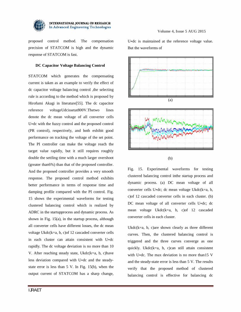
DC Capacitor Voltage Balancing Control
STATCOM which generates the compensating
current is taken as an example to verify the effect of
dc capacitor voltage balancing control ,the selecting
rule is according to the method which is proposed by
Hirofumi Akagi in literature[55]. The dc capacitor
reference voltageUdcissetat800V.Thetwo lines
denote the dc mean voltage of all converter cells
U∗dc with the fuzzy control and the proposed control
(PR control), respectively, and both exhibit good
performance on tracking the voltage of the set point.
The PI controller can make the voltage reach the
target value rapidly, but it still requires roughly
double the settling time with a much larger overshoot
(greater than6%) than that of the proposed controller.
And the proposed controller provides a very smooth
response. The proposed control method exhibits
better performance in terms of response time and
damping profile compared with the PI control. Fig.
15 shows the experimental waveforms for testing
clustered balancing control which is realized by
ADRC in the startupprocess and dynamic process. As
shown in Fig. 15(a), in the startup process, although
all converter cells have different losses, the dc mean
voltage Ukdc(k=a, b, c)of 12 cascaded converter cells
in each cluster can attain consistent with U∗dc
rapidly. The dc voltage deviation is no more than 10
V. After reaching steady state, Ukdc(k=a, b, c)have
less deviation compared with U∗dc and the steady-
state error is less than 5 V. In Fig. 15(b), when the
output current of STATCOM has a sharp change,
U∗dc is maintained at the reference voltage value.
But the waveforms of
(a)
(b)
Fig. 15. Experimental waveforms for testing
clustered balancing control inthe startup process and
dynamic process. (a) DC mean voltage of all
converter cells U∗dc; dc mean voltage Ukdc(k=a, b,
c)of 12 cascaded converter cells in each cluster. (b)
DC mean voltage of all converter cells U∗dc; dc
mean voltage Ukdc(k=a, b, c)of 12 cascaded
converter cells in each cluster.
Ukdc(k=a, b, c)are shown clearly as three different
curves. Then, the clustered balancing control is
triggered and the three curves converge as one
quickly. Ukdc(k=a, b, c)can still attain consistent
with U∗dc. The max deviation is no more than15 V
and the steady-state error is less than 5 V. The results
verify that the proposed method of clustered
balancing control is effective for balancing dc
Gurmeet
Typewritten Text
200
Volume 4, Issue 5 AUG 2015
IJRAET
voltages among three clusters. And it avoids the
overvoltage protection of dc capacitor which cans
make STATCOM stop working. Fig. 17 shows the
experimental waveforms of 12 cells in a phase cluster
for testing individual balancing control which is
realized by shifting the modulation wave vertically in
steady state process. The dc voltages of all cells are
maintained at the given values (800 V) with the small
voltage ripple. This experiment verifies that CPS-
SPWM with the proposed method of individual
voltage control is effective in regulating individual dc
voltages. Results of dc capacitor voltage balancing
control show that the proposed control methods can
coordinate with each other and achieve the best
control effect. They also improve the steady state and
dynamic performance of STATCOM.
Field-programmable gate array
"FPGA" redirects here. It is not to be confused with
Flip-chip pin grid array.
A Stratix IV FPGA from Altera
A field-programmable gate array (FPGA) is an
integrated circuit designed to be configured by a
customer or a designer after manufacturing – hence
"field-programmable". The FPGA configuration is
generally specified using a hardware description
language (HDL), similar to that used for an
application-specific integrated circuit (ASIC) (circuit
diagrams were previously used to specify the
configuration, as they were for ASICs, but this is
increasingly rare).
A Spartan FPGA from Xilinx FPGAs contain
programmable logic components called "logic
blocks", and a hierarchy of reconfigurable
interconnects that allow the blocks to be "wired
together" – somewhat like many logic gates that can
be inter-wired in different configurations. Logic
blocks can be configured to perform complex
combinational functions, or merely simple logic gates
like AND and XOR. In most FPGAs, the logic blocks
also include memory elements, which may be simple
flip-flops or more complete blocks of memory
Gurmeet
Typewritten Text
201

Volume 4, Issue 5 AUG 2015
IJRAET
CONCLUSION
This paper has analyzed the fundamentals of
STATCOM based on multilevel H-bridge converter
with star configuration. And then, the actual H-bridge
cascaded STATCOM rated at 10 kV 2 MVA is
constructed and the novel control methods are also
proposed in detail with fuzzy logic. The proposed
methods has the following characteristics.
1) A PBC theory-based nonlinear controller is first
used in STATCOM with this cascaded structure for
the current loop control, and the viability is verified
by the experimental results with fuzzy.
2) The PR controller is designed for overall voltage
control and the experimental result proves that it has
better performance in terms of response time and
damping profile compared with the fuzzy controller.
3) The ADRC is first used in H-bridge cascaded
STATCOM for clustered balancing control and the
experimental results verify that it can realize
excellent dynamic compensation for the outside
disturbance.
4) The individual balancing control method which is
realized by shifting the modulation wave vertically
can be easily implemented in the FPGA. The
experimental results have confirmed that the
proposed methods are feasible and effective. In
addition, the findings of this study can be extended to
the control of any multilevel voltage source
converter, especially those with H bridge cascaded
structure.
Fig. 17. Experimental waveforms of 12 cells in a-
phase cluster for testing individual balancing control
in the steady-state process.
FUTUREWORK
The application of a new nonlinear control
method based on PBC theory in current loop control
coupled with the dc capacitor voltage balancing
control techniques described in this paper has been
shown to be very effective at improving the steady
state and dynamic performance of H-bridge cascaded
STATCOM, and making the realization of control
methods in DSP and FPGA became easier.
Furthermore, the future work will focus on studying
the control method of H-bridge cascaded STATCOM
under unbalanced and distorted grid voltage. It will
make H-bridge cascaded STATCOM run steadily and
keep the ideal reactive compensation effect under any
conditions.
The difference between the unbalanced and distorted
grid with the balanced and no distorted grid only lies
in that the negative sequence component and the
harmonic component exist in the unbalanced and
distorted grid, but they do not appear in the balanced
and no distorted grid. So, on basis of the research
results in this paper, H-bridge cascaded STATCOM
can still achieve the satisfactory performance under
unbalanced and distorted grid voltage by adding the
Gurmeet
Typewritten Text
202

Volume 4, Issue 5 AUG 2015
IJRAET
negative sequence component controller and the
harmonic component controller in current loop
control, and also the corresponding voltage controller
for restraining the impact of the negative sequence
component on dc capacitor voltage balancing control.
To achieve this objective, in further investigation, the
authors will focus on the work of the following
respects.
1) Under unbalanced voltage, in order to obtain the
negative sequence phase angle, the existing PLL
which only obtains the positive sequence phase angle
in this paper needs to be improved for extracting the
positive sequence synchronizing signal and the
negative sequence synchronizing signal separately.
2) The negative sequence component reference signal
and the harmonic component reference signal also
need to be calculated separately.
3) According to the proposed nonlinear control
method based on PBC theory in this paper, the
negative sequence component controller and the
harmonic component controller will be designed and
added in current loop control.
4) In order to restrain the impact of the negative
sequence component on clustered balancing control,
we will use the method of the zero-sequence voltage
injection according to the dc voltage deviation.
Because zero-sequence voltage has different effects
on three-phase compensation current, but the sum of
these different effects is zero in one cycle.
Based on the previous characteristic, this method can
be used for clustered balancing control under
unbalanced grid voltage. And the proposed ADRC in
this paper will be still used to realize the method of
the zero-sequence voltage injection.
In addition, the proposed method for individual
balancing control in this paper is achieved in the
stage of CPS-SPWM and the dc voltage of each cell
is controlled independently. So, it does not need to
consider the impact of the negative sequence
component. This method will continue to be used in
future work.
APPENDIX
I. DISSIPATION SYSTEM THEORY AND
ENERGY STORAGE FUNCTION
Because passivity theory is an important component
of the dissipation system theory, it is necessary to
know the definition of the dissipation system to prove
that H-bridge cascaded STATCOM is strictly
passive. Moreover, the energy storage function of
system should be selected properly. Let us first recall
the definition of the dissipation system. Then, we will
introduce that how to select the energy storage
function of the system in this paper.
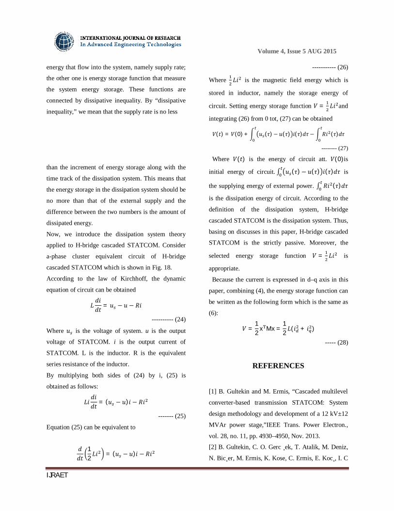
Fig. 18. a-phase cluster equivalent circuit of H-bridge
cascaded STATCOM.
Dissipativity is the fundamental property of physical
system closely related to energy losses and energy
dissipation [54]. The typical example of energy
dissipation system is circuit, in which partial electric
energy and magnetic energy dissipate in the resistor
in the form of heat. To accurately define dissipativity,
it requires two functions: one reflects the rate of
Gurmeet
Typewritten Text
203
Volume 4, Issue 5 AUG 2015
IJRAET
energy that flow into the system, namely supply rate;
the other one is energy storage function that measure
the system energy storage. These functions are
connected by dissipative inequality. By “dissipative
inequality,” we mean that the supply rate is no less
than the increment of energy storage along with the
time track of the dissipation system. This means that
the energy storage in the dissipation system should be
no more than that of the external supply and the
difference between the two numbers is the amount of
dissipated energy.
Now, we introduce the dissipation system theory
applied to H-bridge cascaded STATCOM. Consider
a-phase cluster equivalent circuit of H-bridge
cascaded STATCOM which is shown in Fig. 18.
According to the law of Kirchhoff, the dynamic
equation of circuit can be obtained
퐿푑푖푑푡 = 푢 − 푢 − 푅푖
---------- (24)
Where 푢 is the voltage of system. u is the output
voltage of STATCOM. i is the output current of
STATCOM. L is the inductor. R is the equivalent
series resistance of the inductor.
By multiplying both sides of (24) by i, (25) is
obtained as follows:
퐿푖푑푖푑푡 = (푢 − 푢)푖 − 푅푖
------- (25)
Equation (25) can be equivalent to
푑푑푡
12 퐿푖 = (푢 − 푢)푖 − 푅푖
----------- (26)
Where 퐿푖 is the magnetic field energy which is
stored in inductor, namely the storage energy of
circuit. Setting energy storage function 푉 = 퐿푖 and
integrating (26) from 0 tot, (27) can be obtained
푉(푡) = 푉(0) + 푢 (휏)− 푢(휏) 푖(휏)푑휏 − 푅푖 (휏)푑휏
-------- (27)
Where 푉(푡) is the energy of circuit att. 푉(0)is
initial energy of circuit. ∫ 푢 (휏)− 푢(휏) 푖(휏)푑휏 is
the supplying energy of external power. ∫ 푅푖 (휏)푑휏
is the dissipation energy of circuit. According to the
definition of the dissipation system, H-bridge
cascaded STATCOM is the dissipation system. Thus,
basing on discusses in this paper, H-bridge cascaded
STATCOM is the strictly passive. Moreover, the
selected energy storage function 푉 = 퐿푖 is
appropriate.
Because the current is expressed in d–q axis in this
paper, combining (4), the energy storage function can
be written as the following form which is the same as
(6):
푉 =12 x Mx =
12 퐿(푖 + 푖 )
----- (28)
REFERENCES
[1] B. Gultekin and M. Ermis, “Cascaded multilevel
converter-based transmission STATCOM: System
design methodology and development of a 12 kV±12
MVAr power stage,”IEEE Trans. Power Electron.,
vol. 28, no. 11, pp. 4930–4950, Nov. 2013.
[2] B. Gultekin, C. O. Gerc ¸ek, T. Atalik, M. Deniz,
N. Bic¸er, M. Ermis, K. Kose, C. Ermis, E. Koc¸, I. C
Gurmeet
Typewritten Text
Gurmeet
Typewritten Text
204

Volume 4, Issue 5 AUG 2015
IJRAET
¸ adirci, A. Ac ¸ik, Y. Akkaya, H. Toygar, and S.
Bideci, “Design and implementation of a 154-kV±50-
Mvar transmission STATCOM based on 21-level
cascaded multilevel converter,”IEEE Trans. Ind.
Appl., vol. 48, no. 3, pp. 1030–1045, May/Jun. 2012.
[3] S. Kouro, M. Malinowski, K. Gopakumar, L. G.
Franquelo, J. Pou, J. Rodriguez, B. Wu, M. A. Perez,
and J. I. Leon, “Recent advances and industrial
applications of multilevel converters,”IEEE Trans.
Ind. Electron., vol. 57, no. 8, pp. 2553–2580, Aug.
2010.
[4] F. Z. Peng, J.-S. Lai, J. W. McKeever, and J.
VanCoevering, “A multilevel voltage-source inverter
with separate DC sources for static var generation,”
IEEE Trans. Ind. Appl., vol. 32, no. 5, pp. 1130–
1138, Sep./Oct. 1996.
[5] Y. S. Lai and F. S. Shyu, “Topology for hybrid
multilevel inverter,”Proc. Inst. Elect. Eng.—Elect.
Power Appl., vol. 149, no. 6, pp. 449–458, Nov.
2002.
[6] D. Soto and T. C. Green, “A comparison of high-
power converter topologies for the implementation of
FACTS controllers,”IEEE Trans. Ind. Electron., vol.
49, no. 5, pp. 1072–1080, Oct. 2002.
[7] C. K. Lee, J. S. K. Leung, S. Y. R. Hui, and H. S.-
H. Chung, “Circuit-level comparison of STATCOM
technologies,”IEEE Trans. Power Electron., vol. 18,
no. 4, pp. 1084–1092, Jul. 2003.
[8] H. Akagi, S. Inoue, and T. Yoshii, “Control and
performance of a transformerless cascade PWM
STATCOM with star configuration,” IEEE Trans.
Ind. Appl., vol. 43, no. 4, pp. 1041–1049, Jul./Aug.
2007.
[9] A. H. Norouzi and A. M. Sharaf, “Two control
scheme to enhance the dynamic performance of the
STATCOM and SSSC,”IEEE Trans. Power Del., vol.
20, no. 1, pp. 435–442, Jan. 2005.
[10] C. Schauder, M. Gernhardt, E. Stacey, T.
Lemak, L. Gyugyi, T. W. Cease, and A. Edris,
“Operation of±100 MVAr TVA STATCOM,”IEEE
Trans. Power Del., vol. 12, no. 4, pp. 1805–1822,
Oct. 1997.
[11] C. H. Liu and Y. Y. Hsu, “Design of a self-
tuning PI controller for a STATCOM using particle
swarm optimization,”IEEE Trans. Ind. Electron., vol.
57, no. 2, pp. 702–715, Feb. 2010.
[12] S. Mohagheghi, Y. Del Valle, G. K.
Venayagamoorthy, and R. G. Harley, “A
proportional-integrator type adaptive critic design-
based neurocontroller for a static compensator in a
multimachine power system,” IEEE Trans. Ind.
Electron., vol. 54, no. 1, pp. 86–96, Feb. 2007.
[13] H. F. Wang, H. Li, and H. Chen, “Application of
cell immune response modelling to power system
voltage control by STATCOM,”Proc. Inst. Elect.
Eng. Gener. Transm. Distrib., vol. 149, no. 1, pp.
102–107, Jan. 2002.
[14] A. Jain, K. Joshi, A. Behal, and N. Mohan,
“Voltage regulation with STATCOMs: Modeling,
control and results,”IEEE Trans. Power Del., vol. 21,
no. 2, pp. 726–735, Apr. 2006.
[15] V. Spitsa, A. Alexandrovitz, and E. Zeheb,
“Design of a robust state feedback controller for a
STATCOM using a zero set concept,” IEEE Trans.
Power Del., vol. 25, no. 1, pp. 456–467, Jan. 2010.
[16] C. D. Townsend, T. J. Summers, and R. E. Betz,
“Multigoal heuristic model predictive control
technique applied to a cascaded H-bridge
STATCOM,”IEEE Trans. Power Electron., vol. 27,
no. 3, pp. 1191–1200, Mar. 2012.

Volume 4, Issue 5 AUG 2015
IJRAET
[17] C. D. Townsend, T. J. Summers, J. Vodden, A.
J. Watson, R. E. Betz, and J. C. Clare, “Optimization
of switching losses and capacitor voltage ripple using
model predictive control of a cascaded H-bridge
multilevel STATCOM,”IEEE Trans. Power
Electron., vol. 28, no. 7, pp. 3077–3087, Jul. 2013.
[18] Y. Shi, B. Liu, and S. Duan, “Eliminating DC
current injection in current transformer-sensed
STATCOMs,” IEEE Trans. Power Electron., vol. 28,
no. 8, pp. 3760–3767, Aug. 2013.
[19] B. Singh and S. R. Arya, “Adaptive theory-
based improved linear sinusoidal tracer control
algorithm for DSTATCOM,” IEEE Trans. Power
Electron., vol. 28, no. 8, pp. 3768–3778, Aug. 2013.
[20] S. R. Arya and B. Singh, “Performance of
DSTATCOM using leaky LMS control
algorithm,”IEEE J. Emerging Select. Topics Power
Electron., vol. 1, no. 2, pp. 104–113, Jun. 2013.
[21] P. Petitclair, S. Bacha, and J.-P. Fe rrieux,
“Optimized linearization via feedback control law for
a STATCOM,” in Proc. IEEE Ind. Appl. Soc. Annu.
Meeting, 1997, pp. 880–885.
Gurmeet
Typewritten Text
205
Related Documents