MiNTS Misr National Transport Study Itinerary Itinerary Counterpart Training Program Counterpart Training Program Stage 1 – Knowledge Building Stage Day 2 - Session 1 1 MiNTS Misr National Transport Study What’s GIS? What’s GIS? • Geographic Information System (GIS) is “a computer application used to store, view, and analyze geographical information, especially maps”. (Source: American Heritage Dictionary) 2 A1-60

Welcome message from author
This document is posted to help you gain knowledge. Please leave a comment to let me know what you think about it! Share it to your friends and learn new things together.
Transcript
1
MiNTSMisr National
Transport Study
ItineraryItinerary
Counterpart Training ProgramCounterpart Training Program
Stage 1 – Knowledge Building Stage
Day 2 - Session 1
1
MiNTSMisr National
Transport Study
What’s GIS?What’s GIS?
• Geographic Information System (GIS) is “a computer application used to store, view, and analyze geographical information, especially maps”.
(Source: American Heritage Dictionary)
2
A1-60

2
MiNTSMisr National
Transport Study
Layer and DatasetLayer and Dataset
� There are various geographic features such as administrative boundary, transportation, land use, census result, structures and so force.
� Data types are also various including numerical results of mapping survey, photo image, address and zip code.
� GIS relate all these data and enable cross-layer analysis on computer.computer.
3
MiNTSMisr National
Transport Study
Advantages of GIS compared with Advantages of GIS compared with Paper MapPaper Map
GIS is …• Multiscale
– Zoom in and out freely
• Interactive– Overlay function ease interactive analyses
• Software with Many Applications– Tools such as map editing, geographical analyses,
routing, geocoding etc• Multiple Source
– Many kind of source of information can be • Flexible
– A variety of GIS map applications and frameworks support a wide range of deployment options such as original software or website
4
A1-61
3
MiNTSMisr National
Transport Study
3 functions and views of GIS3 functions and views of GIS
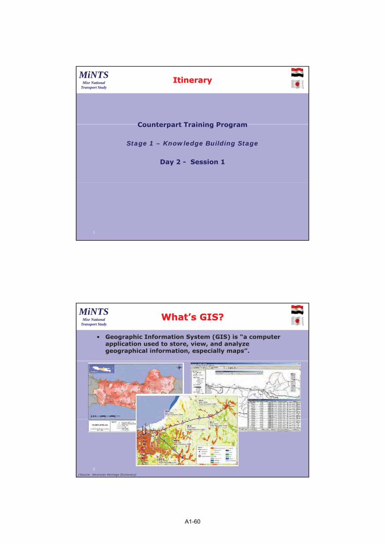
• Geodatabase
– A GIS is a spatial databaseA GIS is a spatial database containing datasets such as features, rasters, attributes, topologies, networks, and so forth.
• Geoprocessing
– A GIS is a set of intelligent maps and other views that show features and feature relationships on the earth’sfeature relationships on the earth s surface.
• Geovisualization
– A GIS is a set of information transformation tools that derive new information from existing datasets.
5
MiNTSMisr National
Transport Study
Type of GIS datasetType of GIS dataset
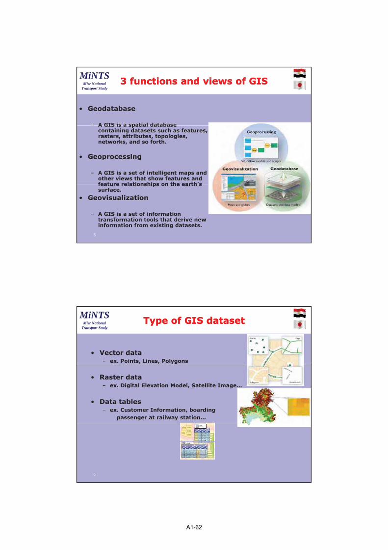
• Vector data – ex. Points, Lines, Polygons
• Raster data – ex. Digital Elevation Model, Satellite Image…
• Data tables – ex. Customer Information, boarding
passenger at railway station…
6
A1-62

4
MiNTSMisr National
Transport Study
VectorVector--based featuresbased features
• Points
• Lines
• Polygons
7
MiNTSMisr National
Transport Study
Coordinate SystemCoordinate System
• Geographic Coordinate System
� Identifying location on earth by longitude and latitude. Although longitude and latitude is identical g gto location on earth, there are several geocodingsystems because of difference or anchoring point.
• Projected Coordinate System
� Since the earth is a deformed sphere, some rules, projection, are required for describing it in flat display or paper.
� Projected coordinate system is based on projections, hence coordinate unit is distanceprojections, hence coordinate unit is distance measure such as meter.
8
A1-63
5
MiNTSMisr National
Transport Study
Coordinate System in Central JavaCoordinate System in Central Java
• Geographic Coordinate System
– Most type of coordinate system can be applied.– Example of coordinate by Longitude and Latitude at Yogyakarta
Tugu station is (110 21’58”E, 7 47’22”S).
• Projected Coordinate System
– Universal Mercator Method (UTM), which divide area by 6 degree longitude, is widely used. Central Java regions are close to the are called “49S”.called 49S .
– “WGS_1984_UTM_Zone_49S” is typical project coordination file for Central Java.
– Example of coordinate by UTM 49S at Yogyakarta Tugu station is(430113m, 9138917m)
9
MiNTSMisr National
Transport Study
Major GIS softwareMajor GIS software
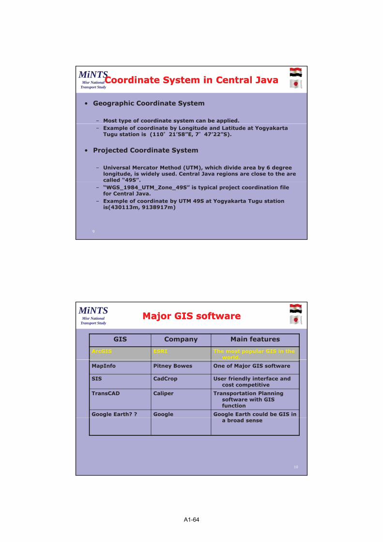
GIS Company Main features
ArcGIS ESRI The most popular GIS in the world.
MapInfo Pitney Bowes One of Major GIS software
SIS CadCrop User friendly interface and cost competitive
TransCAD Caliper Transportation Planning software with GIS function
Google Earth? ? Google Google Earth could be GIS in
10
a broad sense
A1-64

6
MiNTSMisr National
Transport Study
What’s ArcGISWhat’s ArcGIS
• ArcGIS contains various packages for Desktop PC, Server, Developer and Mobile machines and now and now CUBECUBE
11
MiNTSMisr National
Transport Study
ArcGIS Desktop SeriesArcGIS Desktop Series
• ArcViewf h i d t i d– focuses on comprehensive data use, mapping, andanalysis.
• ArcEditor– adds advanced geographic editing and data creation.
• ArcInfoi l f i l GIS d k i i– is a complete, professional GIS desktop containingcomprehensive GIS functionality, including rich geoprocessing tools.
12
A1-65

7
MiNTSMisr National
Transport Study
Applications included in Applications included in ArcViewArcView
Applications Features
ArcMap The main application in ArcGIS is ArcMap, which is used for all mapping and editing tasks as well as for map-based query and analysis. It’s the primary application for all map based tasks including cartography, map analysis, and editing.
ArcCatalog,tool box
The Arc Catalog application helps users organize and manage all geographic information, such as maps, globes, data files, geodatabases, geo processing toolboxes, metadata and GIS services
13
metadata, and GIS services.
ModelBuilder
The Model Builder interface provides a graphical modeling framework for designing and implementing geo processing models that can include tools, scripts, and data.
MiNTSMisr National
Transport Study
ArcMapArcMap
– ArcMap is main application of ArcGIS consisting of many controls, toolbars and object libraries.
– User can show and edit map with powerful GUI (graphical user interface).
14
A1-66
8
MiNTSMisr National
Transport Study
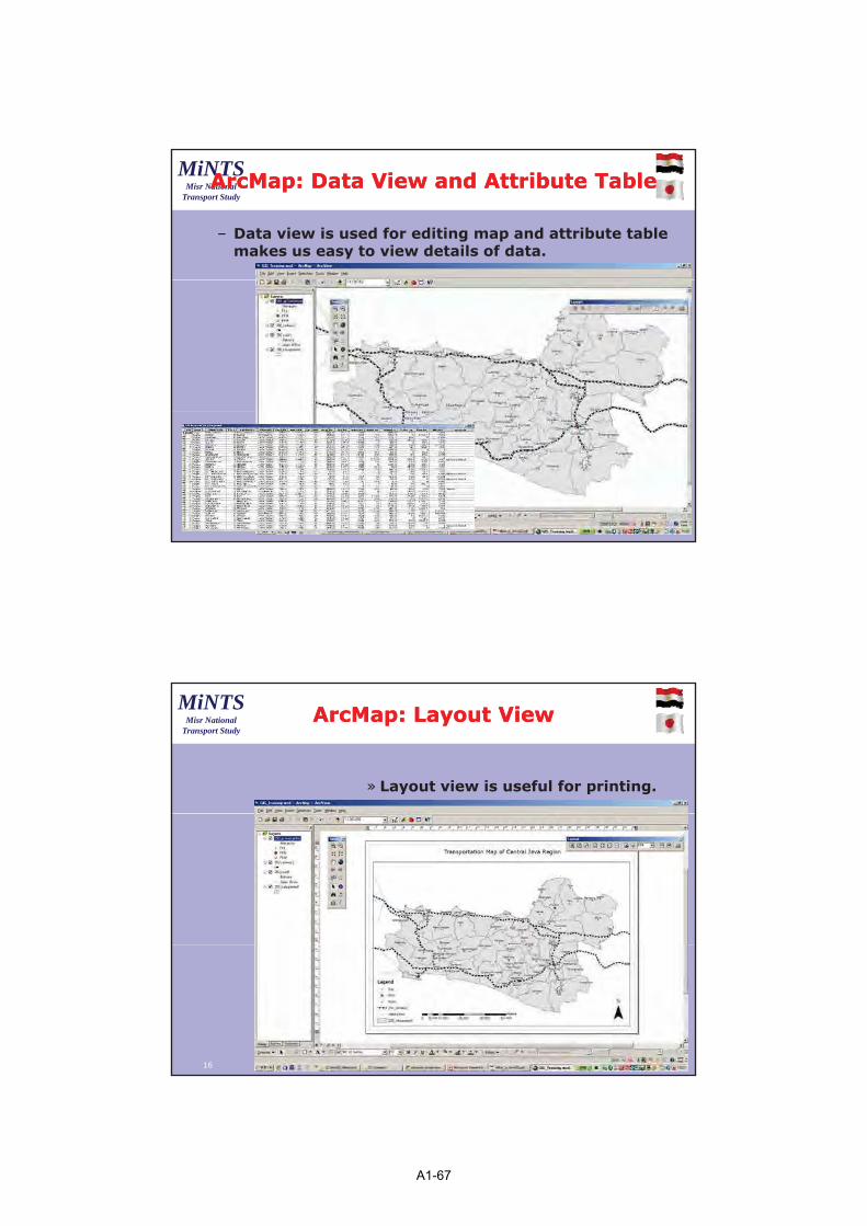
ArcMap: Data View and Attribute TableArcMap: Data View and Attribute Table
– Data view is used for editing map and attribute table makes us easy to view details of data.
15
MiNTSMisr National
Transport Study
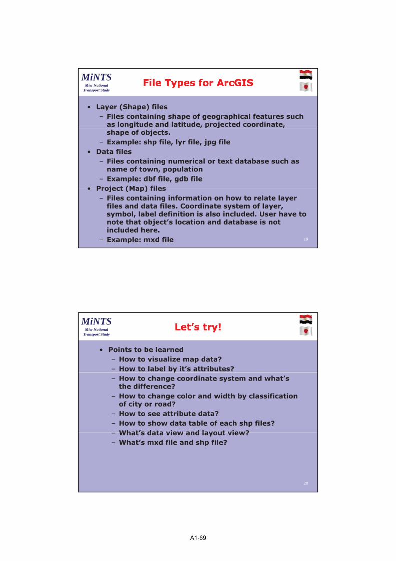
ArcMapArcMap: Layout View: Layout View
» Layout view is useful for printing.
16
A1-67

9
MiNTSMisr National
Transport Study
ArcCatalogArcCatalog
– ArcCatalog is powerful application, especially for processing geographic data, “geo processing” with explorer like GUI and tool box.
17
MiNTSMisr National
Transport Study
Model BuilderModel Builder
– In case user requires complicated geographic data processing, “geo processing”, model builder play important role visualizing flow of process.
– Users who only conduct simple processing, model builder is not essential.
18
A1-68
10
MiNTSMisr National
Transport Study
File Types for File Types for ArcGISArcGIS
• Layer (Shape) files– Files containing shape of geographical features such
as longitude and latitude, projected coordinate, g p jshape of objects.
– Example: shp file, lyr file, jpg file• Data files
– Files containing numerical or text database such as name of town, population
– Example: dbf file, gdb file• Project (Map) files
19
• Project (Map) files– Files containing information on how to relate layer
files and data files. Coordinate system of layer, symbol, label definition is also included. User have to note that object’s location and database is not included here.
– Example: mxd file
MiNTSMisr National
Transport Study
Let’s try!Let’s try!
• Points to be learned– How to visualize map data?– How to label by it’s attributes? y– How to change coordinate system and what’s
the difference?– How to change color and width by classification
of city or road?– How to see attribute data?– How to show data table of each shp files?
What’s data view and layout view?
20
– What s data view and layout view?– What’s mxd file and shp file?
A1-69
11
MiNTSMisr National
Transport Study Let’s try! (1) LabelingLet’s try! (1) Labeling and Symbolizingand Symbolizing
• Visualize kabupaten, city, road and railway in one map using the following data.
File type File Name Data Type
Kabupaten kabupaten.shp Area
Road road.shp Line
Railway railway.shp Line
21
City activecenter.shp Point
MiNTSMisr National
Transport Study
Let’s try! (1) LabelingLet’s try! (1) Labeling and Symbolizingand Symbolizing
• How to symbolize and label features– Open ArcGIS by clicking Start -> Program -> ArcGIS -
> ArcMapp– Choose “A new empty map”.– Right click “Layers” in the table of contents– Choose “Add data” and browse the geographic shape
file which you want to open.– Change symbol by double clicking and choosing
“Symbology” tab.Adding label by double clicking and choosing
22
– Adding label by double clicking and choosing “Labels” tab.
– After labeling and symbolizing, please save mxd file
A1-70

12
MiNTSMisr National
Transport Study
Let’s try! (1) LabelingLet’s try! (1) Labeling and Symbolizingand Symbolizing
• How to remove unnecessary symbol– Choose layer of “road”.– Double click and choose “Symbology” tab.Double click and choose Symbology tab.– From left box, choose “Categoly” and “Unique Value”.– From “Value field” pull down menu, choose “Bahasa”.– Push “Add All Values” bottun.– Choose symbol except “Jalan Arteri” using shift key.– Right click and choose “Remove Value(s)”.– Only Arterial Road will be shown in the map.– Please try to make a map like example answers
23
MiNTSMisr National
Transport Study
Let’s try! (1) Example AnswersLet’s try! (1) Example Answers
Pati
Tayu
Comal
BloraSlawi
TegalDemak
Kudus
Lasem
Weleri
KendalBatangBrebes
Jepara
Juwana
Kersana
Rembang
SemarangWiradesaAdiwerna
Pemalang
Pecangaan
Ketanggungan
24
CepuBoja
Bawen
Kroya
Jaten
Kajen
Wates
Gubug
Sragen
Wangon
Bantul
Sleman Klaten
Secang
Godong
Klampok
Cilacap
Kebumen
GombongMungkid
Parakan
Ungaran
Sokaraja
Banyumas
Majenang
Delanggu
Wonosobo
Kutoarjo
Magelang
Muntilan
Wonosari
Wonogiri
Ambarawa
Sukorejo
Salatiga
Boyolali
Prambanan
Bobotsari
Ajibarang
Kartasura
Sukoharjo
Surakarta
Purworejo
Borobudur
Purwodadi
Purwantoro
Mertoyudan
Temanggung
Yogyakarta
Tawangmangu
Purbalingga
Karanganyar
Randudongkal
gg g
Banjarnegara
A1-71
13
MiNTSMisr National
Transport Study
Let’s try! (3) Using Layout viewLet’s try! (3) Using Layout view
• Add legend, north arrow and scale bar using layout view– Push “Layout View” button in the left bottom
corner.– In the top tool bar, push “Insert” -> “Legend” to
show legend of map.– Text, North arrow and Scale bar is also added
selecting each menu from “Insert” menu.– Please try to make a map like example answer
25
Please try to make a map like example answer
A1-72

1
MiNTSMisr National
Transport Study
ItineraryItinerary
Counterpart Training ProgramCounterpart Training Program
Stage 1 – Knowledge Building Stage
Day 2 - Session 2
1
MiNTSMisr National
Transport Study
Joining and Relating map Joining and Relating map withwithdatabasedatabase -- 11
• One of the key function of GIS is to join and relate variety of data and analyses them easily.
• Usually shp file and it’s corresponding dbf file contain attributes data.
• You can find the attribute data by right clicking layer and choose “Open Attribute Table”.
2
A1-73

2
MiNTSMisr National
Transport Study
JoiningJoining and Relating map with and Relating map with database database -- 22
• Joining map with tables / maps– The joined attributes will be saved in the dataset’s attributes
table.– The joined attributes can be labeled and calculated.– Both data field and spatial location can be used for joining maps
or tables.
3
MiNTSMisr National
Transport Study
JoiningJoining and Relating map with and Relating map with database database -- 33
• Relating map with tables / maps– Relating do NOT append attributes.– Relating only stores the relationship between tables.– The related records are accessed on demand, when you select a
feature or record in the original table or map.
4
A1-74

3
MiNTSMisr National
Transport Study
JoiningJoining and Relating map and Relating map with database with database -- 44
• Data Consistency is sometimes crucial…
– Data have to be identical. Neither difference of expression nor space is allowed. Description have to be same to join or relate data.
– Example: “Surakarta”, “Solo”, “Kota Solo”, “Kdy.Solo”, “Kdy Solo”, “KdySolo”?
– Numerical ID is recommended to join data.
5
MiNTSMisr National
Transport Study
(1) Joining and Relating map (1) Joining and Relating map withwith databasedatabase
• One(many)-to-one(many) relationship– Joining: One-to-one and Many-to-one only– Relating: One-to-one, Many-to-one, One-to-many, Many-to Many
can be used.
Kota PopulationSemarang 1,468,292Solo 512,898Yogyakarta 443,112
Kota Station
Kota Population StationSemarang 1,468,292 Tawang? Poncol?Solo 512,898 Purwosari? Balapan? Jebres?
Semarang TawangSemarang PoncolSolo PurwosariSolo BalapanSolo Jebres
Yogyakarta TuguYogyakarta Lempuyangan
pYogyakarta 443,112 Tugu? Lempuyangan?
Example of one-to-many relationship
6
A1-75

4
MiNTSMisr National
Transport Study
GeoprocessingGeoprocessing
• Geoprocessing is one of the unique feature of GIS which edit data by geographical conditions.
• Geoprocessing is the methodical execution of a sequence of operations on geographic data to create new information. The process you perform may be routine, for example, to help you convert a number of files from one format to another.
7
MiNTSMisr National
Transport Study
GeoprocessingGeoprocessing
The following are typical types of Geoprocessings:– Intersect
• Computes the geometric intersection of two coveragesComputes the geometric intersection of two coverages,where only those features in the area common to both coverages will be preserved.
– Dissolve• Merges adjacent polygons, lines, or regions that have the
same value for a specified item.
8
A1-76
5
MiNTSMisr National
Transport Study
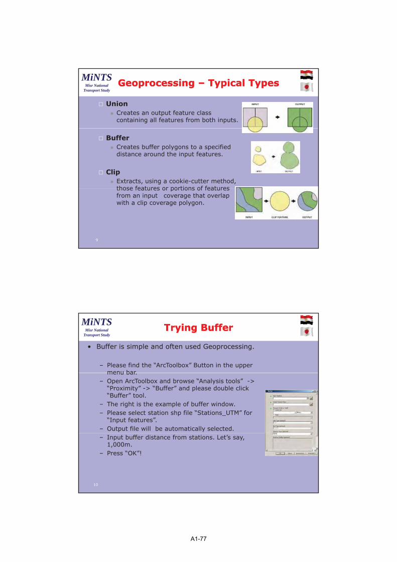
GeoprocessingGeoprocessing –– Typical TypesTypical Types
� Union� Creates an output feature class
containing all features from both inputs.
� Buffer� Creates buffer polygons to a specified
distance around the input features.
� Clip� Extracts, using a cookie-cutter method,
those features or portions of featuresthose features or portions of features from an input coverage that overlap with a clip coverage polygon.
9
MiNTSMisr National
Transport Study
Trying BufferTrying Buffer
• Buffer is simple and often used Geoprocessing.
– Please find the “ArcToolbox” Button in the upper menu barmenu bar.
– Open ArcToolbox and browse “Analysis tools” -> “Proximity” -> “Buffer” and please double click “Buffer” tool.
– The right is the example of buffer window.– Please select station shp file “Stations_UTM” for
“Input features”.– Output file will be automatically selected.– Input buffer distance from stations. Let’s say,
1,000m.– Press “OK”!
10
A1-77
6
MiNTSMisr National
Transport Study
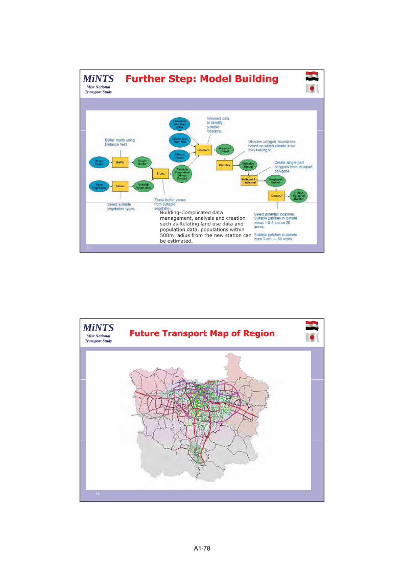
Further Step: Model Further Step: Model BuildingBuilding
11
Building-Complicated data management, analysis and creation such as Relating land use data and population data, populations within 500m radius from the new station can be estimated.
MiNTSMisr National
Transport Study
Future Transport Map of RegionFuture Transport Map of Region
12
A1-78
7
MiNTSMisr National
Transport Study
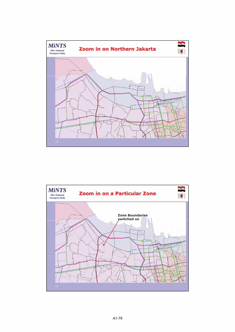
Zoom in on Northern JakartaZoom in on Northern Jakarta
13
MiNTSMisr National
Transport Study
Zoom in on a Particular ZoneZoom in on a Particular Zone
Zone Boundaries switched on
14
A1-79

8
MiNTSMisr National
Transport Study
Highlight the ZoneHighlight the Zone
At present only limited data linked to thetransport model but that will change
15
MiNTSMisr National
Transport Study
GeoprocessingGeoprocessing Union Using CUBEUnion Using CUBE
16
A1-80

9
MiNTSMisr National
Transport Study
SpecifySpecify GeoprocessingGeoprocessing
17
MiNTSMisr National
Transport Study
Add new Zone Data for CairoAdd new Zone Data for Cairo
Add�New�Zone
18
A1-81
10
MiNTSMisr National
Transport Study
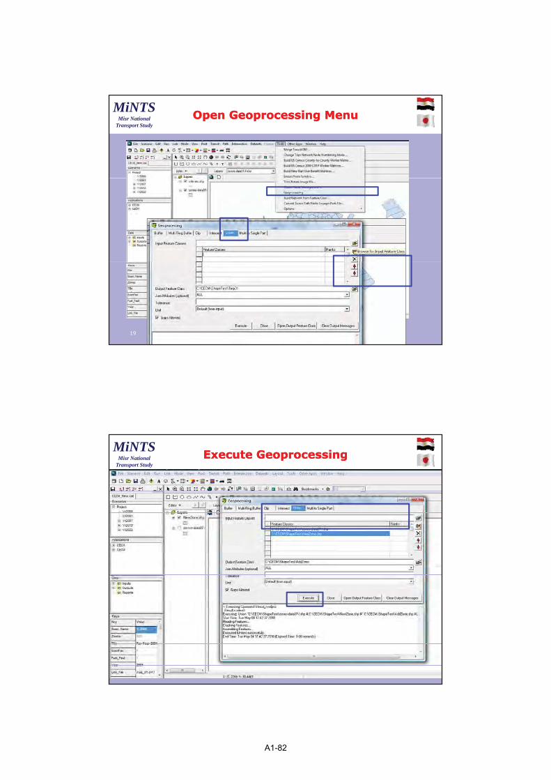
OpenOpen GeoprocessingGeoprocessing MenuMenu
19
MiNTSMisr National
Transport Study
ExecuteExecute GeoprocessingGeoprocessing
20
A1-82

11
MiNTSMisr National
Transport Study
NewNew Zone Added to MapZone Added to Map
21
A1-83

1
MiNTSMisr National
Transport Study
ItineraryItinerary
Counterpart Training ProgramCounterpart Training Program
Stage 1 – Knowledge Building Stage
Day 2 - Session 3
1
MiNTSMisr National
Transport Study
CUBECUBE----CitilabsCitilabs
• Citilabs was created several years ago via a merger of UAG and the software division of an English C lti CConsulting Company
• 2200 sites in more than 70 countries use its products for transportation planning
• Citilabs is an Authorized ESRI Business Partner, utilizing ArcGISEngine and other ESRI products.
Cube Dynasim
2
A1-84
2
MiNTSMisr National
Transport Study
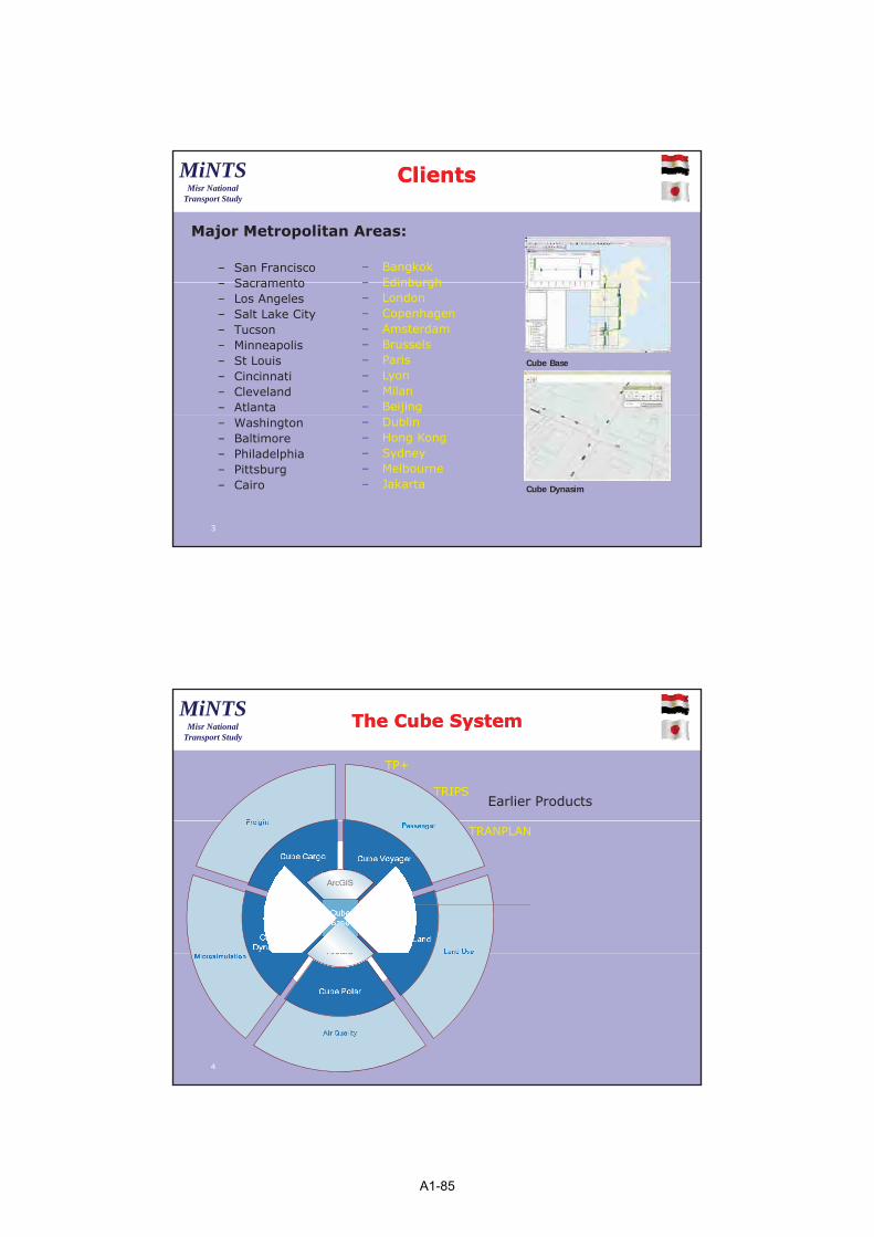
ClientsClients
Major Metropolitan Areas:
– San FranciscoSacramento
– Bangkok– Edinburgh– Sacramento
– Los Angeles– Salt Lake City– Tucson– Minneapolis– St Louis– Cincinnati– Cleveland– Atlanta
Cube Base
– Edinburgh– London– Copenhagen– Amsterdam– Brussels– Paris– Lyon– Milan– Beijing
– Washington– Baltimore– Philadelphia– Pittsburg– Cairo Cube Dynasim
– Dublin– Hong Kong– Sydney– Melbourne– Jakarta
3
MiNTSMisr National
Transport Study
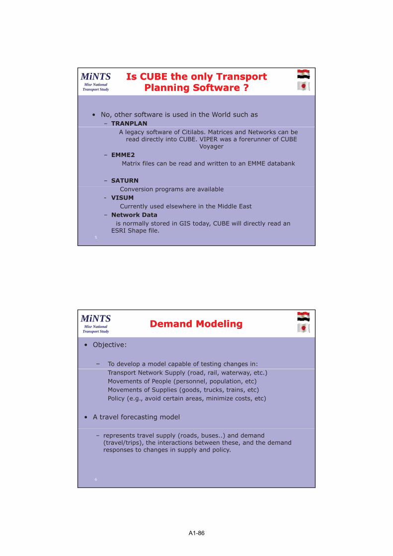
The Cube SystemThe Cube System
TP+
TRIPSEarlier Products
place
product
pricetargetmarket
ArcGIS
ArcGIS
ArcGIS
ArcGIS
TRANPLAN
promotion
ArcGIS
4
A1-85
3
MiNTSMisr National
Transport Study
Is CUBE the only Transport Is CUBE the only Transport Planning Software ?Planning Software ?
• No, other software is used in the World such as – TRANPLAN
A legacy software of Citilabs. Matrices and Networks can be read directly into CUBE. VIPER was a forerunner of CUBE
Voyager– EMME2
Matrix files can be read and written to an EMME databank
– SATURNConversion programs are available
- VISUMCurrently used elsewhere in the Middle East
– Network Data is normally stored in GIS today, CUBE will directly read an
ESRI Shape file.5
MiNTSMisr National
Transport Study
DemandDemand ModelingModeling
• Objective:
– To develop a model capable of testing changes in:Transport Network Supply (road, rail, waterway, etc.)Movements of People (personnel, population, etc)Movements of Supplies (goods, trucks, trains, etc)Policy (e.g., avoid certain areas, minimize costs, etc)
• A travel forecasting model
– represents travel supply (roads, buses..) and demand (travel/trips), the interactions between these, and the demand responses to changes in supply and policy.
6
A1-86
4
MiNTSMisr National
Transport Study
Elements of a Demand ModelElements of a Demand Model
1. The Model: – Various equations reflecting travel behavior
How frequently one travelsHow frequently one travelsWhere one travels
What mode..
2. The Software:– Applies ‘The Model’ Equations
3 The Data:
Some of this we have discussed already but we are now looking at the material in the context of a transport model.
3. The Data: – Describes the supply and the demand
Socio-DemographicsLand Use
Networks…
7
MiNTSMisr National
Transport Study
Methodological ApproachesMethodological Approaches
Cube Voyager easily applies to ANY form of Transport Model :
– The ‘Four-Step’ model– The Four-Step model
– Modified ‘Four-Step’ models
– Tour-Based Models
– Activity Based Models
U b M d l– Urban Models
– Regional Models
– National Models
8
A1-87
5
MiNTSMisr National
Transport StudyThe ‘FourThe ‘Four--Step’ ModelStep’ Model
1. Trip Generation:
– Estimate how many trips (Productions) are made by each household for each trip purpose (commuting, shopping…)
– Estimate how many trips (Attractions) are attracted to eachEstimate how many trips (Attractions) are attracted to each location (shopping centers, work places..)
– Results in Production/Attraction Vectors2. Trip Distribution:
– Estimate how many trips go from a location to all other locations
– Results in Production/Attraction Matrices
3. Modal Choice: – Given that someone will travel from one location to another,
compare the travel options and select a mode– Results in Origin/Destination Trip Matrices by Mode
4. Assignment: – Route the travel onto public transport services and roadways
9
MiNTSMisr National
Transport Study
Transport Modeling TerminologyTransport Modeling Terminology
• LINK• NODE• ZONE/TAZ
• MATRIX• GRAVITY MODEL• COSTZONE/TAZ
• CENTRIOD• NETWORK• ZONAL DATA• PRODUCTIONS• ATTRACTIONS • TRIP TABLE
COST• PATH BUILDING• SKIM/SKIMMING• LOS• VC RATIO
Now for some important Now for some important CUBE Terminology.CUBE Terminology.
A1-88

6
MiNTSMisr National
Transport Study
CUBE Terminology CUBE Terminology –– the Catalogsthe Catalogs
• The Catalog– The Catalog File is the only file which you must g y y
remember its name and location.– The Catalog is the ‘root’ of a model. Everything else is
linked to it.– The Catalog tracks all the components of a model
• Applications (Model Processes)• Model Keys (User Input Data)
Scenario Data (Unique Sets of Keys)• Scenario Data (Unique Sets of Keys)
11
MiNTSMisr National
Transport Study
ApplicationsApplications
Applications– The Applications are the Model Processes.
A single Catalog may have many Applications– A single Catalog may have many Applications• Passenger Forecasting• Freight Forecasting• Land-Use Forecasting• Sub-Area Analysis• Impact Studies
Th A li ti fil i i l hi h t k d t– The Application file is a single page which tracks dataflows and organizes modeling functions. These functions may be either from Cube Libraries or User Defined.
– Application files may be nested to provide model structure.12
A1-89

7
MiNTSMisr National
Transport Study
Starting CubeStarting Cube
The ‘Welcome to Cube’ Screen– Used to Access a Catalog– Easy access to the most recent y
Catalog
1. Double-Click the Cube Icon to Access the Welcome Screen
2. Click ‘Cancel’ to open Cube without opening a Catalogwithout opening a Catalog
13
MiNTSMisr National
Transport Study
Create a CatalogCreate a Catalog
1. Select File > New
2. Choose ‘New Catalog’
3. Save the new Catalog to: ???
4. Scenario-Manager opens for the new Catalog along the left-side of the window.
14
A1-90

8
MiNTSMisr National
Transport Study
Back to the CUBE Programs ?Back to the CUBE Programs ?
•Base•VoyagerToday
•Analysis•Avenue•Land•The Geodatabase•The Cairo Model, including a GIS example
Today Next Session
•Scripting•An Example
Tomorrow-Scripting
15
MiNTSMisr National
Transport Study
CUBE BaseCUBE Base
DropDown Menu
Scenario Pane
FLOWCHARTFLOWCHART
Application Pane
Data Pane
Key Pane
16
A1-91

9
MiNTSMisr National
Transport Study
Catalogue KeysCatalogue Keys
17
MiNTSMisr National
Transport Study
CUBE MODEL LEVELSCUBE MODEL LEVELS
Go to next level
18
A1-92

10
MiNTSMisr National
Transport Study
Next Level Down has the ProgramsNext Level Down has the Programs
Further Discussion during practical example
19
MiNTSMisr National
Transport Study
The Voyager ProgramsThe Voyager Programs
Pilot Program
FratarFratar
Highway
Network
Matrix
Distribution
Generation
Public Transport
20
A1-93

11
MiNTSMisr National
Transport Study
PilotPilot
• The Pilot program is the basic driver for Cube Voyager application programs.
• Most users will use Pilot only to invoke the individual programs in the order desired.
• Pilot can check the return codes of the individual programs, invoke system commands, perform complex mathematical.
• Use in loops and conditional branching application• Use in loops and conditional branching, application programs can be run in any order desired.
21
MiNTSMisr National
Transport Study
PilotPilot--An ExampleAn Example
• Through the Pilot Program the model will follow one of two Paths
22
A1-94

12
MiNTSMisr National
Transport Study
GenerationGeneration
• Resident Workers in Income Class by Employment Category
• Resident StudentsInputInput----Traffic Traffic
Zone DataZone Data
• Employment Opportunities in Income Class by Employment Category
• Student Places
OutputOutput------ZonalZonal TripTrip
• Productions by Income Class by Trip Purpose• Attractions by Income Class by Trip Purpose
ZonalZonal TripTripEndsEnds
23
MiNTSMisr National
Transport Study
GenerationGeneration -- ExampleExample
24
A1-95

13
MiNTSMisr National
Transport Study
NetworkNetwork
Reads input network files of various formats: ASCII records, standard database in dBASE style (DBF), Cube geodatabasenetworks, or any Cube Voyager, TP+, MINUTP, Tranplan, or , y y g , , , p ,
TRIPS binary network format.
Generates a data record for each unique node and each link found in any of the input files.
A valid node record, the Network program requires a node variable, named N.
A valid link record, the Network program requires an A-node, named A, and a B-node, named B. Each A-node and B-node must
exist on a node record.
25
MiNTSMisr National
Transport Study
NetworkNetwork ----ExampleExample
Link Group 1 and 2 referred to Road ClassLink Group 3 in combination with Link Group 1 and 2 referred to MRT
Link Group 1-3 from SITRAMP, now there is a new field Link Class26
A1-96
14
MiNTSMisr National
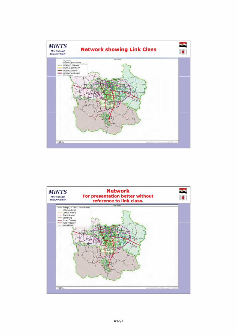
Transport Study
Network showing Link ClassNetwork showing Link Class
27
MiNTSMisr National
Transport Study
NetworkNetworkFor presentation better without For presentation better without
reference to link class.reference to link class.
28
A1-97

15
MiNTSMisr National
Transport Study
DistributionDistribution
• Productions by Income Class by Trip Purpose by Income Class
Input--Zonal Data
• Impedance Functions• Network Travel Skims
Output---Travel
• Travel Matrices by Income Class by Trip Purpose by Income Class
TravelMatrix
29
MiNTSMisr National
Transport Study
Trip Distribution, the StructureTrip Distribution, the Structure
)*/()(1
��
�n
jijijjiij TTAPTrip Af
Where :P = the number of trip productions for a zone.A = the number of trip attractions for a zone.T = the travel impedance factor between zones.i = the production zone.j = the attraction zone.n = the number of zones.
This states that the trip productions in zone I will be distributed to each zoneThis states that the trip productions in zone I will be distributed to each zone according to the relative attractiveness of zone J. Each J’s attractiveness isdetermined by the product of its attractions and some function of the spatial separation between i and j. The sum of the these products for all j’s (relative to i)is obtained . Each j will then be given a pro rata share of the productions for ibased upon its attractiveness.
30
A1-98
16
MiNTSMisr National
Transport Study
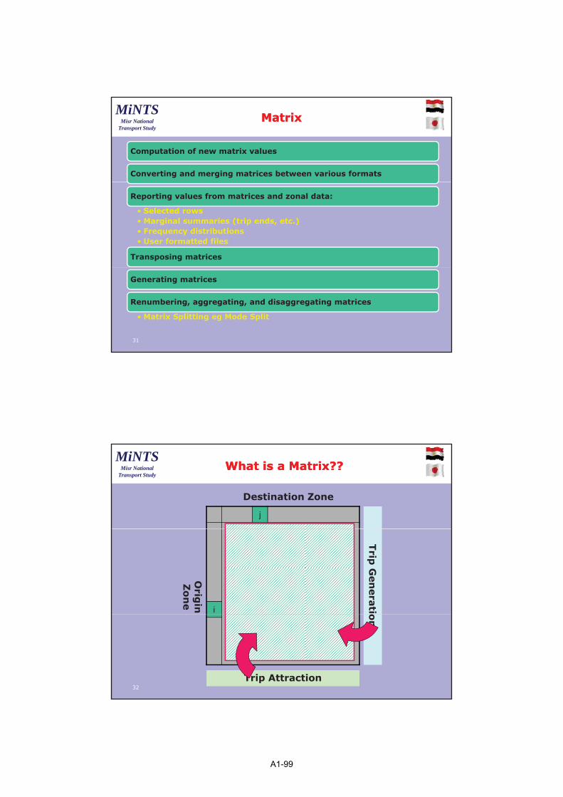
MatrixMatrix
Computation of new matrix values
Converting and merging matrices between various formats
Reporting values from matrices and zonal data:
• Selected rows• Marginal summaries (trip ends, etc.)• Frequency distributions• User formatted files
Transposing matrices
Generating matrices
Renumbering, aggregating, and disaggregating matrices
• Matrix Splitting eg Mode Split
31
MiNTSMisr National
Transport Study
What is a Matrix??What is a Matrix??
j
Destination Zone
i
Orig
inZ
on
e
Trip
Gen
era
ti
Trip Attraction
on
32
A1-99

17
MiNTSMisr National
Transport Study
FratarFratar
• Starting Matrix
Inputs• Column and Row Factors
Outputs
• Revised Matrix with same distribution but with new row and column totals
Outputs
33
MiNTSMisr National
Transport Study
FratarFratar ProcedureProcedure
Zone 1 2 3 Total
1 57 24 19 100
Start Matrix
2 64 106 30 200
3 102 61 137 300
Total 223 191 186 600
Target 240 200 160 600
After Several Iterations
Zone 1 2 3 Total
1 60 25 16 102
2 70 190 26 206
3 113 64 118 292
Total 240 200 160 600
Target is achieved in new column totals with little change in row totals
34
A1-100

18
MiNTSMisr National
Transport Study
HighwayHighway
• Networks• Associated Link and Node Files
Inputs
• Associated Link and Node Files• Toll Files• Turn Penalties• Node Descriptions
• Travel Matrices
• Travel Impedances
Outputs
• Loaded Network• Link Volumes• Intersection Analysis
35
MiNTSMisr National
Transport Study
Highway Node Prior to AssignmentHighway Node Prior to Assignment
Click on this then this
36
A1-101

19
MiNTSMisr National
Transport Study
Highway Node After AssignmentHighway Node After Assignment
Traffic Volume andSignal Settings
37
MiNTSMisr National
Transport Study
Public TransportPublic Transport
• Network File
Inputs
• Line File• Associated Line Data
• Fares• Mode and Operator Descriptions
• Access Links• Travel Matrices by Mode
• Travel Impedances
Outputs
• Travel Impedances• Loaded Network
• Link Volumes• Line Volumes
38
A1-102

20
MiNTSMisr National
Transport Study
Public TransportPublic Transport--Walk Access Links Walk Access Links to PT Routesto PT Routes
39
A1-103
1
MiNTSMisr National
Transport Study
ItineraryItinerary
Counterpart Training ProgramCounterpart Training Program
Stage 1 – Knowledge Building Stage
Day 3 - Session 1
1
MiNTSMisr National
Transport Study
The CUBE Demonstration ProgramThe CUBE Demonstration Program
• Before we start today
• Make sure that you have the Cubetown application installed correctly on your computer
• This way you can follow some of the material directly on your computer
2
A1-104

2
MiNTSMisr National
Transport Study
TheThe GeoDatabaseGeoDatabase
Feature Datasets
TransportNetworks
Data stored in columns suchcolumns such
as any database
GEODATABASE
ESRRI ArcGIS 9.2 personal Geodatabaseformat3
MiNTSMisr National
Transport Study
Geo Database StructureGeo Database Structure
4
A1-105
3
MiNTSMisr National
Transport Study
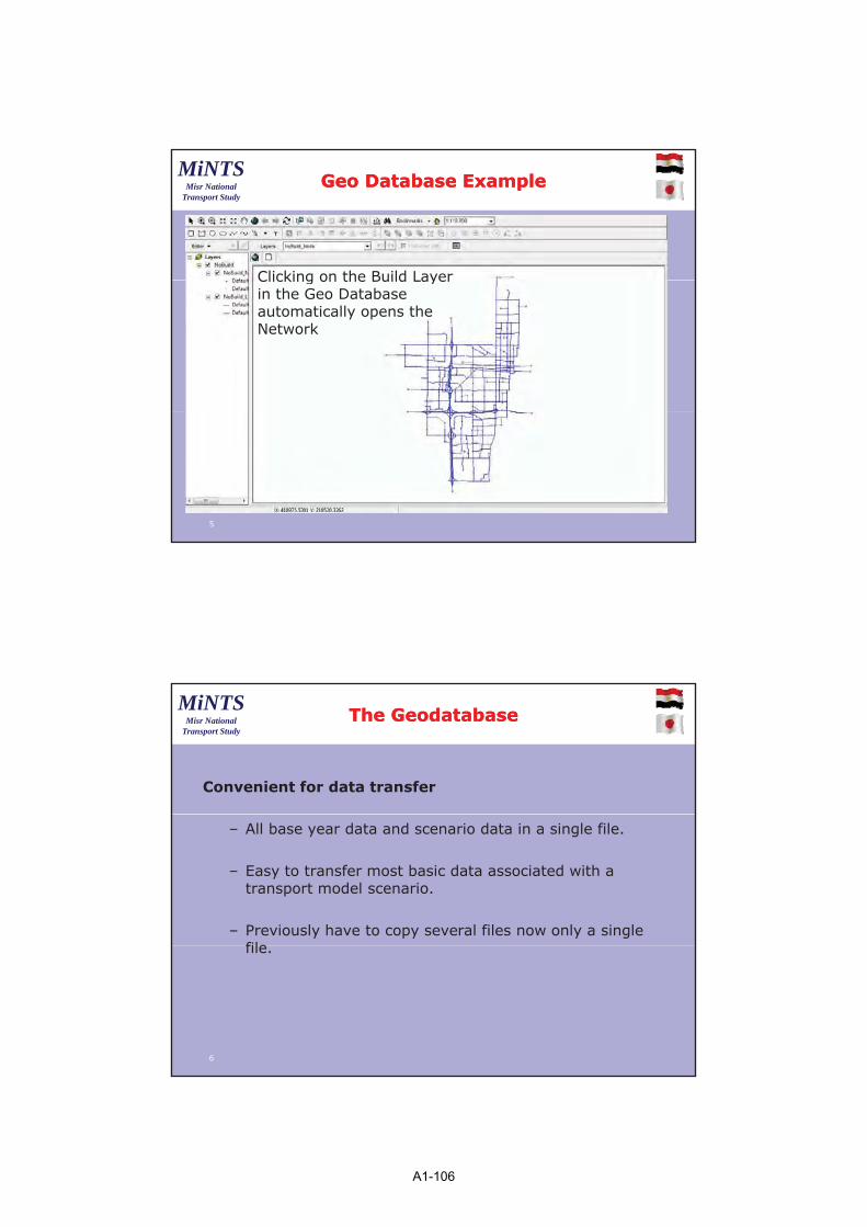
Geo Database ExampleGeo Database Example
Clicking on the Build LayerClicking on the Build Layer in the Geo Database automatically opens the Network
5
MiNTSMisr National
Transport Study
TheThe GeodatabaseGeodatabase
Convenient for data transfer
– All base year data and scenario data in a single file.
– Easy to transfer most basic data associated with a transport model scenario.
– Previously have to copy several files now only a single filefile.
6
A1-106

4
MiNTSMisr National
Transport Study
CUBE Voyager ExtensionsCUBE Voyager Extensions
• Analyst - Voyager Extension
A V E i• Avenue – Voyager Extension
• Land –a new type of model that links land use and the real estate market.
• Cargo - Voyager Extension
7
MiNTSMisr National
Transport Study
AnalystAnalyst
• Earlier Travel Matrix• Count Data
Inputs• Vehicle Counts• Passenger Counts
Outputs
• Updated Travel Matrices that matches Counts both Vehicles and or Passengers
Outputs
8
A1-107

5
MiNTSMisr National
Transport Study
TypicalTypical ScreenlinesScreenlines in a Cityin a City
9
MiNTSMisr National
Transport Study
The ProcessThe Process
• Comparison across screenline shows a large difference between assignment and traffic counts
• Input in available traffic counts
• Improve the match between traffic counts and model by using the maximum likelihood procedure.
10
A1-108
6
MiNTSMisr National
Transport Study
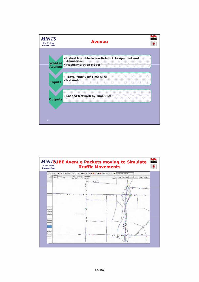
AvenueAvenue
What is
• Hybrid Model between Network Assignment and Animation
• MesoSimulation ModelAvenue
• MesoSimulation Model
Inputs
• Travel Matrix by Time Slice• Network
Outputs• Loaded Network by Time Slice
11
MiNTSMisr National
Transport Study
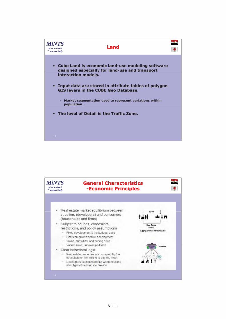
CUBE Avenue Packets moving to Simulate CUBE Avenue Packets moving to Simulate Traffic MovementsTraffic Movements
12
A1-109

7
MiNTSMisr National
Transport Study
A Pause Live DemonstrationA Pause Live Demonstration
• In Model CUBETOWN
• Select Avenue Application
• Select Scenario – Build Road
• Click on Dynamic Loads
• Post – Packet Animation
• Post Packet File from Build Road Directory
13
MiNTSMisr National
Transport Study
Different Application of AvenueDifferent Application of Avenue
• Used extensively in the development of emergency evacuation procedure
• Used to develop for Houston, USA an emergency evacuation in case of Hurricane
• Used in Bangkok to develop emergency evacuation procedures for Major Government Centre in case of emergency event such as the Centre becoming involved in a major protest event.
14
A1-110
8
MiNTSMisr National
Transport Study
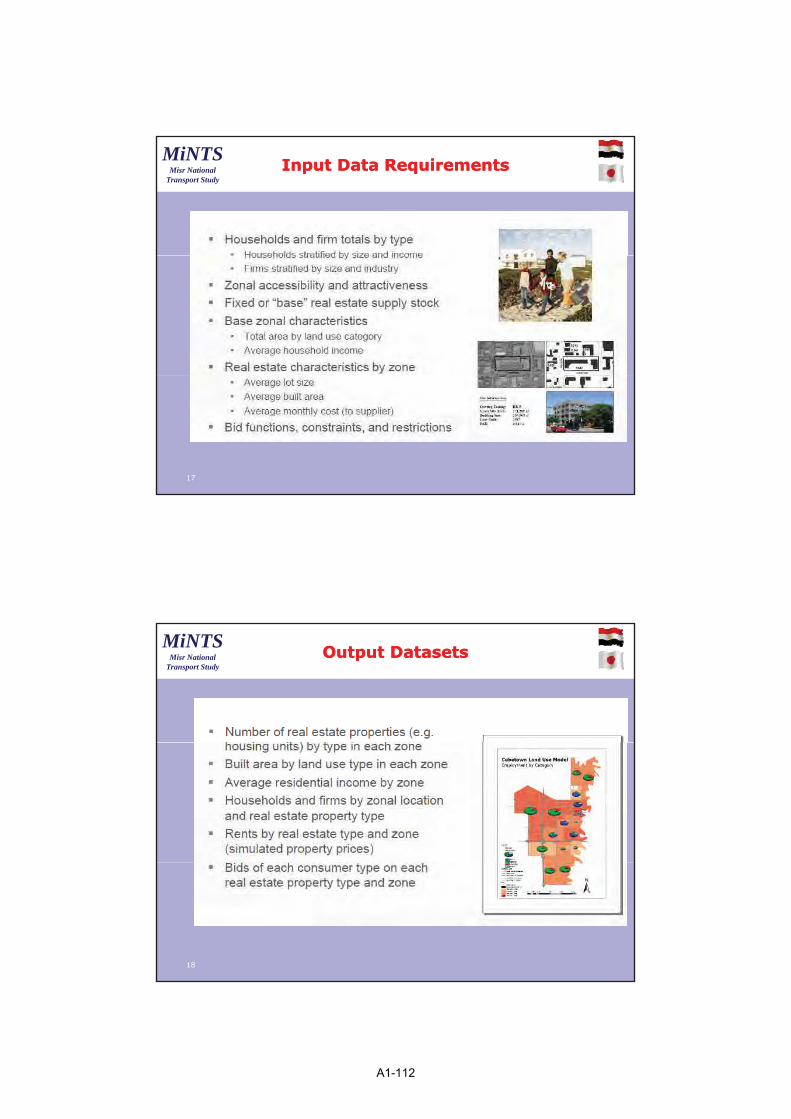
LandLand
• Cube Land is economic land-use modeling software designed especially for land-use and transport interaction models.
• Input data are stored in attribute tables of polygon GIS layers in the CUBE Geo Database.
– Market segmentation used to represent variations within population.
• The level of Detail is the Traffic Zone.
15
MiNTSMisr National
Transport Study
General CharacteristicsGeneral Characteristics--Economic PrinciplesEconomic Principles
16
A1-111
9
MiNTSMisr National
Transport Study
Input Data RequirementsInput Data Requirements
17
MiNTSMisr National
Transport Study
Output DatasetsOutput Datasets
18
A1-112

10
MiNTSMisr National
Transport Study
Technical SpecificationsTechnical Specifications
19
MiNTSMisr National
Transport Study
Land Bidding FunctionsLand Bidding Functions
20
A1-113

11
MiNTSMisr National
Transport Study
Estimation of various Bid FunctionsEstimation of various Bid Functions
21
MiNTSMisr National
Transport Study
Land SummaryLand Summary
22
A1-114
12
MiNTSMisr National
Transport Study
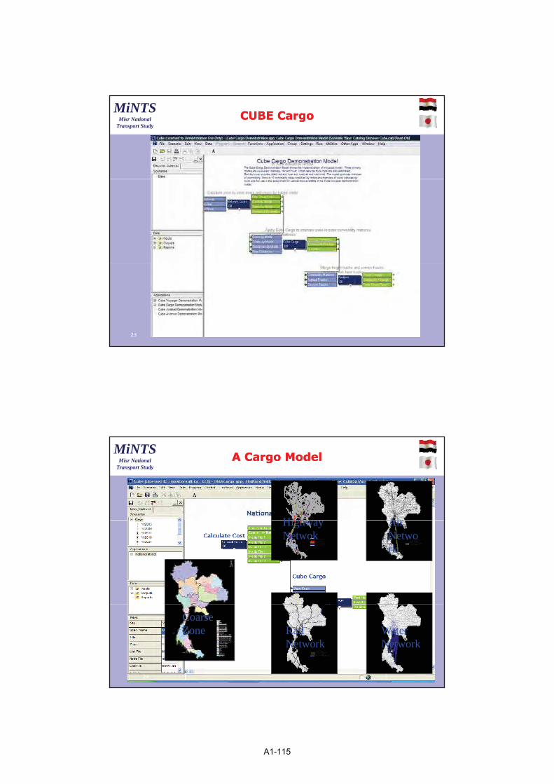
CUBE CargoCUBE Cargo
23
MiNTSMisr National
Transport Study
Hi h Ai
A Cargo ModelA Cargo Model
HighwayNetwok
AirNetwork
CoarseZone Rail
NetworkWater Network
24
A1-115

13
MiNTSMisr National
Transport Study
CargoCargo
What is
• Model to estimate Cargo Flows based on Production and Consumptions
• Model to estimate service vehicle flowsCargo
• Model to estimate service vehicle flows
Inputs
• Socio Economic Data• Network Characteristics• Calibrated Freight Parameters
Outputs• Loaded Network flows in terms of tonnes of products
25
MiNTSMisr National
Transport Study
CargoCargo –– Key Features Key Features CUBE ProductionsCUBE Productions
NONO CargoCargo
11 AgricultureAgriculture
22 FoodstuffsFoodstuffs
33 Solid minerals fuelsSolid minerals fuels
44 Petroleum productsPetroleum products44 Petroleum productsPetroleum products
55 Ores and metal wasteOres and metal waste
66 Metal productsMetal products
77 Building materialsBuilding materials
88 FertilizersFertilizers
99 ChemicalsChemicals
1010 Manufactured goodsManufactured goods
26
A1-116

14
MiNTSMisr National
Transport Study
Building CostsBuilding Costs
Highway Network Cost Water Network Cost
Build Cost MatrixBuild Cost MatrixRail Network Cost
27
MiNTSMisr National
Transport Study
PRODUCTIONPRODUCTION
Cargo ProductionCargo Production
Model DescriptionModel Description
Model ParameterModel Parameter
Z l D tZ l D tINPUTINPUT
Zonal DataZonal Data
Manipulation DataManipulation Data
Base VolumeBase Volume
N UN UFILEFILE
28
A1-117
15
MiNTSMisr National
Transport Study
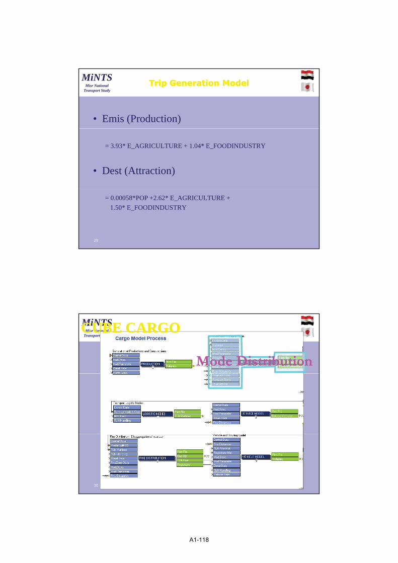
Trip Generation ModelTrip Generation Model
• Emis (Production)
= 3.93* E_AGRICULTURE + 1.04* E_FOODINDUSTRY
• Dest (Attraction)
= 0.00058*POP +2.62* E_AGRICULTURE +
1.50* E_FOODINDUSTRY
29
MiNTSMisr National
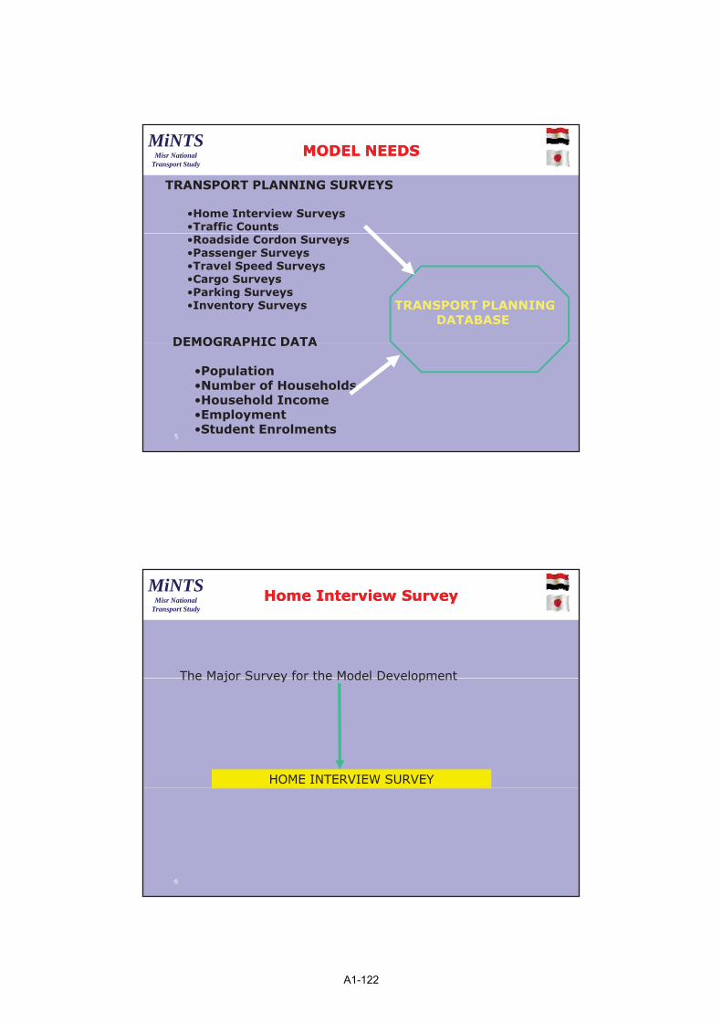
Transport StudyCUBE CARGOCUBE CARGO
Mode DistributionMode Distribution
30
A1-118

16
MiNTSMisr National
Transport Study
Trip Length DistributionsTrip Length Distributions
31
MiNTSMisr National
Transport Study
Sample Deterrence FunctionSample Deterrence Function
32
A1-119

1
MiNTSMisr National
Transport Study
ItineraryItinerary
Counterpart Training ProgramCounterpart Training Program
Stage 1 – Knowledge Building Stage
Day 3 - Session 2
1
MiNTSMisr National
Transport Study
WHY Did CAIRO NEED A TRANSPORT MODEL ??22
GREATER CAIROGREATER CAIRO URBAN URBANTRANSPORTTRANSPORT TMODELTMODEL
• Many Proposed Transport Projects
• Limited Resources
• Evaluate Best Use of Resources
2
Resources
• Rank Projects in Order of Priority
A1-120

2
MiNTSMisr National
Transport Study
MODEL NEEDSMODEL NEEDS
Transport Database
Software
Model Development
3
MiNTSMisr National
Transport Study
THE PREVIOUS SLIDE IS ONE THAT WE HAVE SEEN SEVERAL TIMES SO FAR BUT IT REMAINS IMPORTANT TO UNDERSTAND
FOCUS OF PRESENTATIONFOCUS OF PRESENTATION
TIMES SO FAR BUT IT REMAINS IMPORTANT TO UNDERSTAND THAT THIS IS THE ESSENCE OF ANY TRANSPORT MODEL….THIS PRESENTATION WILL FOCUS ON THE DEVELOPMENT OF THE THE CAIRO EXTENDED CITY MODEL or CECM, THE CAIRO EXTENDED CITY MODEL or CECM, developed during the CREATS project in 2001 and 2002.
4
A1-121
3
MiNTSMisr National
Transport Study
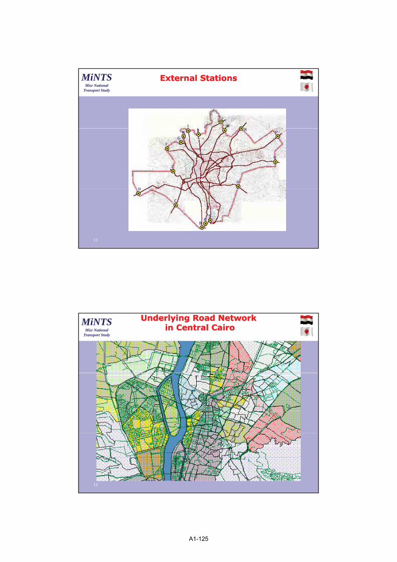
TRANSPORT PLANNING SURVEYS
•Home Interview Surveys•Traffic Counts
MODEL NEEDSMODEL NEEDS
•Roadside Cordon Surveys•Passenger Surveys•Travel Speed Surveys•Cargo Surveys•Parking Surveys•Inventory Surveys
DEMOGRAPHIC DATA
TRANSPORT PLANNINGDATABASE
DEMOGRAPHIC DATA
•Population•Number of Households•Household Income•Employment•Student Enrolments
5
MiNTSMisr National
Transport Study
The Major Survey for the Model Development
Home Interview SurveyHome Interview Survey
The Major Survey for the Model Development
HOME INTERVIEW SURVEY
6
A1-122

4
MiNTSMisr National
Transport Study
Model FlowchartModel Flowchart
7
MiNTSMisr National
Transport Study
Aspects of the Transport ModelAspects of the Transport Model
A. Network and Zoning System
B. Trip Generation
C. Trip Distribution
D. Modal Split
E. Trucks and External Trip Tables
F Trip Table DevelopmentF. Trip Table Development
G. Assignment /Calibration
H. Future Year Results
I. Snapshots of the Transport Model8
A1-123

5
MiNTSMisr National
Transport Study
AA-- Zoning System and NetworkZoning System and Network
ZONING SYSTEM
--- For Cairo Transport Model, based on some Combined Shiakhas - 464 Internal Zones and 19 External Stations
9
MiNTSMisr National
Transport Study
Traffic Zones in Central CairoTraffic Zones in Central Cairo
10
A1-124
6
MiNTSMisr National
Transport Study
External StationsExternal Stations
11
MiNTSMisr National
Transport Study
Underlying Road NetworkUnderlying Road Networkin Central Cairoin Central Cairo
12
A1-125
7
MiNTSMisr National
Transport Study
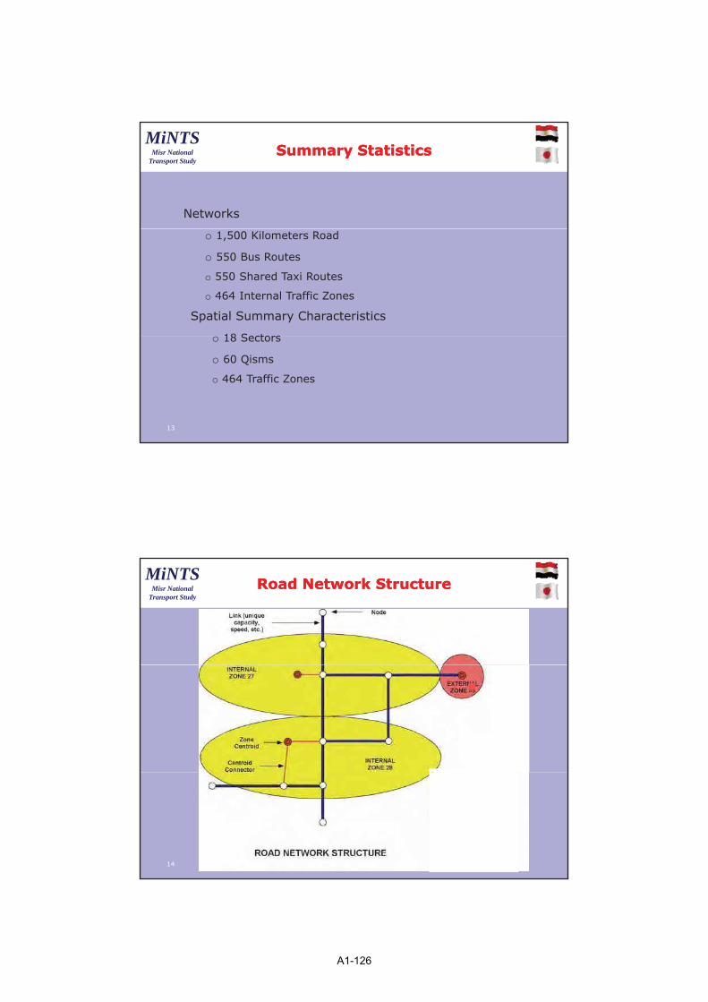
Networks
SummarySummary StatisticsStatistics
o 1,500 Kilometers Road
o 550 Bus Routes
o 550 Shared Taxi Routes
o 464 Internal Traffic Zones
Spatial Summary Characteristics
18 Sectors
13
o 18 Sectors
o 60 Qisms
o 464 Traffic Zones
MiNTSMisr National
Transport Study
Road Network StructureRoad Network Structure
14
A1-126
8
MiNTSMisr National
Transport Study
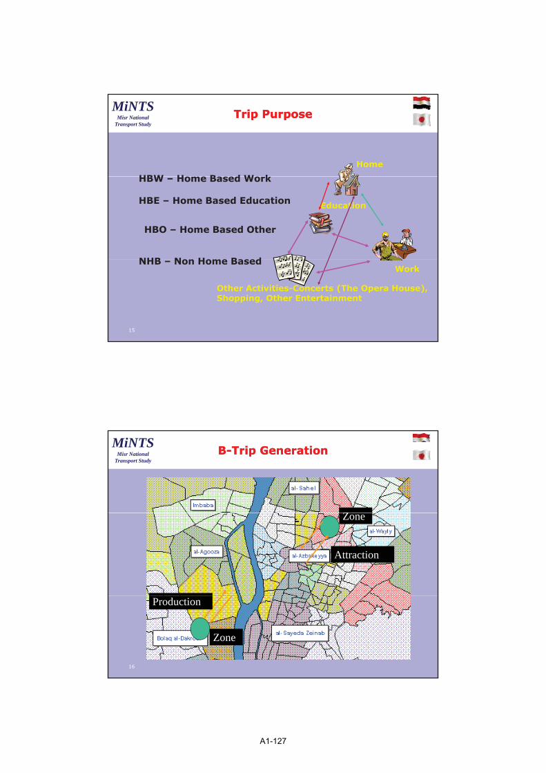
Trip PurposeTrip Purpose
HBW H B d W k
Home
HBO – Home Based Other
HBW – Home Based Work
HBE – Home Based Education
NHB N H B d
Education
NHB – Non Home BasedWork
Other Activities-Concerts (The Opera House),Shopping, Other Entertainment
15
MiNTSMisr National
Transport Study
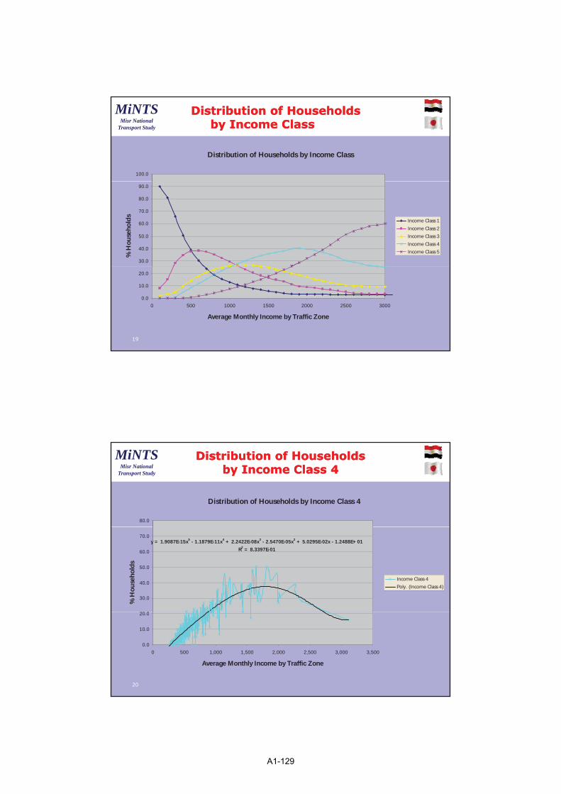
BB--Trip GenerationTrip Generation
Z
Attraction
Zone
16
Production
Zone
A1-127

9
MiNTSMisr National
Transport Study
Trip Production Rate for Each Disaggregate Group or Bin
For Each Trip Purpose HBW etc
Category Analysis of Trip GenerationCategory Analysis of Trip Generation
HOUSEHOLD SIZEINCOME CLASS 1 2 3 4 etc
1 ?? ?? ?? ??2 ?? ?? ?? ??3 ?? ?? ?? ??4 ?? ?? ?? ??5 ?? ?? ?? ??
17
MiNTSMisr National
Transport Study
Income Class RangeIncome Class Range
Class Income Range(LE per Month in 2001 Value)
1 <3002 300-5003 500-1,0004 1,000-2,0005 >2,000
18
A1-128
10
MiNTSMisr National
Transport Study
Distribution of Households by Income Class
100.0
Distribution of HouseholdsDistribution of Householdsby Income Classby Income Class
30.0
40.0
50.0
60.0
70.0
80.0
90.0
% H
ou
seh
old
s
Income Class 1
Income Class 2
Income Class 3
Income Class 4
Income Class 5
0.0
10.0
20.0
0 500 1000 1500 2000 2500 3000
Average Monthly Income by Traffic Zone
19
MiNTSMisr National
Transport Study
Distribution of Households Distribution of Households by Income Class by Income Class 44
Distribution of Households by Income Class 4
80.0
y = 1.9087E-15x5 - 1.1879E-11x
4 + 2.2422E-08x
3 - 2.5470E-05x
2 + 5.0295E-02x - 1.2488E+ 01
R2 = 8.3397E-01
20 0
30.0
40.0
50.0
60.0
70.0
% H
ou
seh
old
s
Income Class 4
Poly. (Income Class 4)
20
0.0
10.0
20.0
0 500 1,000 1,500 2,000 2,500 3,000 3,500
Average Monthly Income by Traffic Zone
A1-129

11
MiNTSMisr National
Transport Study
Distribution of Households Distribution of Households by HH Sizeby HH Size
Distribution of Households by Household Size
45.0
15.0
20.0
25.0
30.0
35.0
40.0
% H
ou
seh
old
s HH_Size_1
HH_Size_2
HH_Size_3
HH_Size_4
HH_Size_5
HH_Size_6
HH_Size_7
21
0.0
5.0
10.0
2.0 2.5 3.0 3.5 4.0 4.5 5.0 5.5 6.0 6.5
Average Household Size
MiNTSMisr National
Transport Study
Distribution of Households by Distribution of Households by Household Size Household Size 77
Distribution of Households by Household Size 7
y = 0.5275x5 - 11.172x
4 + 92.461x
3 - 370.18x
2 + 719.58x - 543.55
R2 = 0.7936
50 0
60.0
10 0
20.0
30.0
40.0
50.0
% H
ou
seh
old
s
HH_Size_7
Poly. (HH_Size_7)
22
0.0
10.0
2.0 2.5 3.0 3.5 4.0 4.5 5.0 5.5 6.0
Average Household Size
A1-130

12
MiNTSMisr National
Transport Study
Observed Percentage Distribution of Observed Percentage Distribution of HouseholdsHouseholds
Household Size
Income Class 1 2 3 4 5 6 7
1 2.5 5.1 5.2 5.5 5.0 3.6 4.12 3.0 4.2 5.2 6.7 6.5 4.2 4.73 0.8 2.1 2.4 4.0 3.2 2.1 2.14 0 4 1 4 2 1 3 4 2 7 1 9 1 8
23
4 0.4 1.4 2.1 3.4 2.7 1.9 1.85 0.1 0.4 0.7 1.1 0.8 0.5 0.4
MiNTSMisr National
Transport Study
Household Size
Modeled Percentage Distribution of Modeled Percentage Distribution of HouseholdsHouseholds
Income Class 1 2 3 4 5 6 7
1 2.1 4.7 5.1 5.7 5.2 3.8 4.42 3.0 4.1 5.2 6.8 6.5 4.3 4.73 1.0 2.3 2.4 3.9 3.1 2.0 1.94 0 6 1 7 2 2 3 3 2 6 1 7 1 54 0.6 1.7 2.2 3.3 2.6 1.7 1.55 0.3 0.5 0.7 1.0 0.7 0.4 0.4
24
A1-131

13
MiNTSMisr National
Transport Study
TRIP ATTRACTION are a
Trip AttractionsTrip Attractions
f(Employment Characteristics by Class,Households, Student Enrolments)
e.g. AHBW= a*Primary Employment+b*Secondary Employment+c*Tertiary Employment
where a, b, and c are calibration constantswhere a, b, and c are calibration constants
25
MiNTSMisr National
Transport Study
HBW Trip Attraction CoHBW Trip Attraction Co--efficientsefficients
Income Class
Primary Employment
Secondary Employment
TertiaryEmployment R 2
1 1.205 0.215 0.465 0.97
2 - 0.690 0.627 0.97
3 - 0.187 0.564 0.92
26
4 - 0.008 0.733 0.84
5 - - 0.281 0.69
A1-132

14
MiNTSMisr National
Transport Study
Other Trip Attraction CoOther Trip Attraction Co--efficientsefficients
P C t t St d t University H h ld Tertiary R 2Purpose Constant Students yStudents Household y
Employment R 2
HBE - 2.129 2.336 - - 0.99
HBO 292.8 - - - 0.406 0.67
27
NHB - - - 0.00918 0.175 0.54
MiNTSMisr National
Transport Study
CC-- Trip DistributionTrip Distribution
Traffic Zone
Traffic Zone
Trip Generation
28
Traffic Zone
Trip Generation
Trip Distribution
Tij � Pi*Aj*f(Costij)
F Factor
A1-133

15
MiNTSMisr National
Transport Study
Typical F Factor Curve
What is a F Factor CurveWhat is a F Factor Curve
F F
act
or
Cost (Impedance)
29
MiNTSMisr National
Transport Study
F Factor Function F Factor Function
Where :Cij - Weighted Generalized Cost of Travel; anX1 and X2 are Calibration Constants
)exp()( 21
ijX
ijij CXCCF �
X1 and X2 are Calibration Constants
30
A1-134
16
MiNTSMisr National
Transport Study
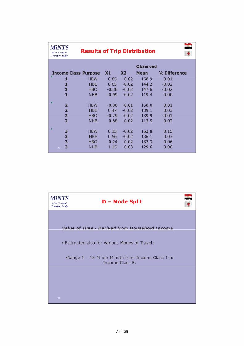
Results of Trip DistributionResults of Trip Distribution
Observed
Income Class Purpose X1 X2 Mean % Difference1 HBW 0 85 -0 02 168 9 0 011 HBW 0.85 -0.02 168.9 0.011 HBE 0.65 -0.02 144.2 -0.021 HBO -0.36 -0.02 147.6 -0.021 NHB -0.99 -0.02 119.4 0.00
2 HBW -0.06 -0.01 158.0 0.012 HBE 0.47 -0.02 139.1 0.032 HBO -0 29 -0 02 139 9 -0 012 HBO 0.29 0.02 139.9 0.012 NHB -0.88 -0.02 113.5 0.02
3 HBW 0.15 -0.02 153.8 0.153 HBE 0.56 -0.02 136.1 0.033 HBO -0.24 -0.02 132.3 0.063 NHB 1.15 -0.03 129.6 0.0031
MiNTSMisr National
Transport Study
Value of Time - Derived from Household Income
DD –– Mode SplitMode Split
• Estimated also for Various Modes of Travel;
•Range 1 – 18 Pt per Minute from Income Class 1 to Income Class 5.
32
A1-135
17
MiNTSMisr National
Transport Study
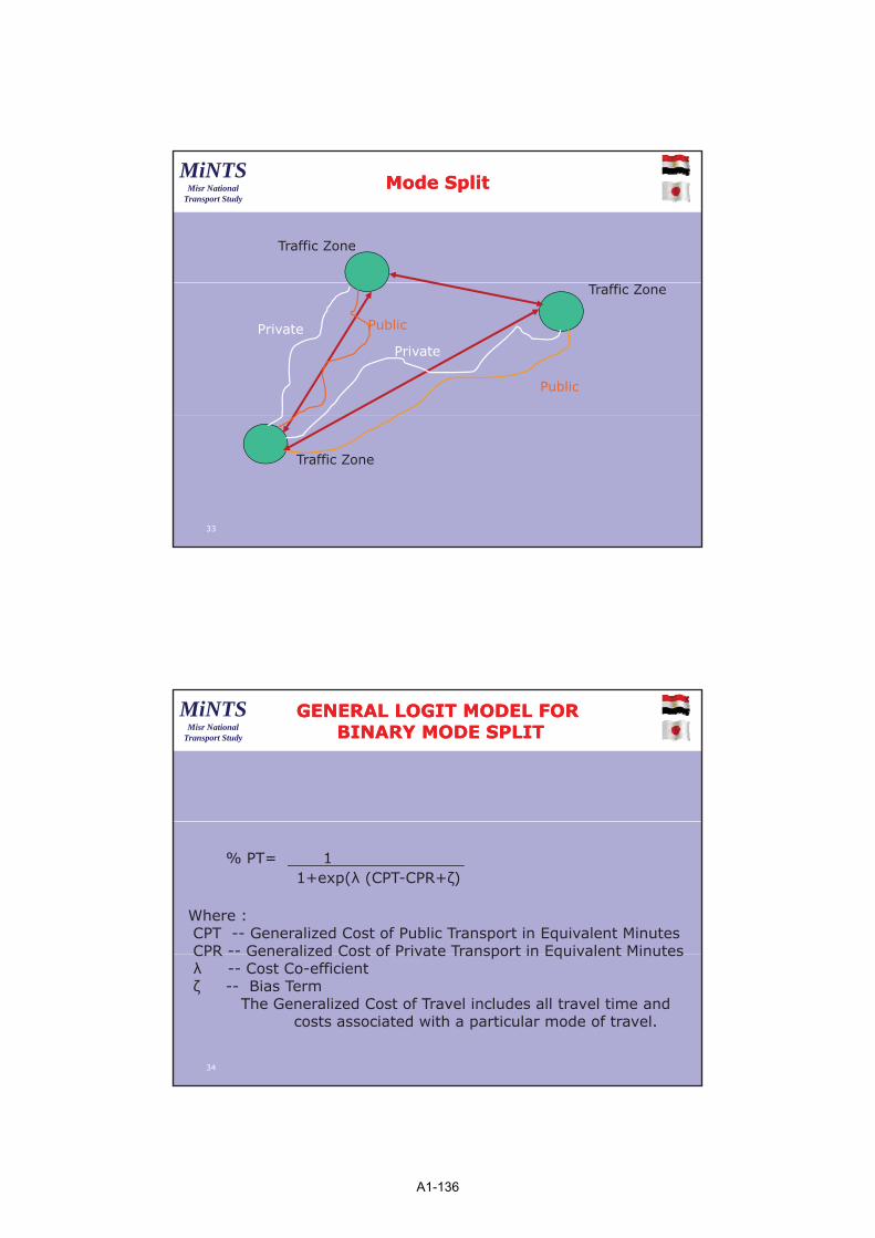
Traffic Zone
Mode SplitMode Split
Traffic Zone
Public
Public
Private
Private
Traffic Zone
33
MiNTSMisr National
Transport Study
GENERAL LOGIT MODEL FORGENERAL LOGIT MODEL FORBINARY MODE SPLITBINARY MODE SPLIT
% PT= 11+exp(� (CPT-CPR+�)
Where :CPT -- Generalized Cost of Public Transport in Equivalent MinutesCPR -- Generalized Cost of Private Transport in Equivalent MinutesCPR Generalized Cost of Private Transport in Equivalent Minutes� -- Cost Co-efficient� -- Bias Term
The Generalized Cost of Travel includes all travel time andcosts associated with a particular mode of travel.
34
A1-136

18
MiNTSMisr National
Transport StudyTypical Mode Split CurveTypical Mode Split Curve
35
MiNTSMisr National
Transport Study
Overall % Modal SplitOverall % Modal Split
Mode of TravelMode of Travel ModelModel ObservedObserved
S i l B 8 4 8 4Special Bus(Employee/School)
8.4 8.4
Public Transport(CTA Bus, Shared Taxi etc)
62.9 63.2
Car 20.6 20.4
36
Taxi 8.1 8.0
Total 100.0 100.0
A1-137

19
MiNTSMisr National
Transport Study
•Small Trucks
EE –– Trucks and Externals Trucks and Externals
oPick Up/Utility – Goods Vehicleo2 Axle Trucks
•Large Truckso 3 Axle Truckso >3 Axle Truckso >3 Axle Trucks
37
MiNTSMisr National
Transport Study
External Trip Tables by Truck Category
Development of TruckDevelopment of TruckTrip Tables Trip Tables
Internal Roadside Survey
Cargo Survey
Initial Estimate Of Truck Trips By Truck Category
Matrix Estimation
Traffic Counts at 100 Sites
Truck Trip Table by Category
38
A1-138

20
MiNTSMisr National
Transport Study
Truck Calibration Simulated Vs Truck Calibration Simulated Vs ObservedObserved
35,000
40,000
15,000
20,000
25,000
30,000
ulat
ed T
ruck
PC
U V
olum
e
Small Trucks (Less than 3 Axles)
Large Trucks (3 and More Axles)
0
5,000
10,000
0 5,000 10,000 15,000 20,000 25,000 30,000 35,000Observed Truck PCU Volume
Sim
u
Data source: JICA Study Team. Data are a comparison of observed and modeled daily pcu volumes at study
area traffic count locations.
39
MiNTSMisr National
Transport Study
Small Trucks Large Trucks
Estimation of Future Truck Estimation of Future Truck Trip EndsTrip Ends
Y=aXb Y= a+bX
WhereY = Internal Trip Ends(pcu) per zoneX = Secondary Employment for SmallX = Total Employment per sq km for Large Trucks
a, b = Calibration Constants
TFuture=TBase*(TEst in Future/ TEst in Base)
40
A1-139

21
MiNTSMisr National
Transport Study
Truck Trip End ParametersTruck Trip End Parameters
Category Constant
(a)
Secondary Employment (b)
Total Employment per
S K (b)
Correlation Coefficient
Sq Km (b)
Small Truck 0.0266 - 1.015 0.77
Large Truck 69.5 0.021 - 0.69
41
In the case of External Trip Tables Derived from Cordon Surveys--- 5 Categories
• Car•Taxi•Bus•Small Truck•Large Truck
--- Future Growth derived from Overall Trip Growth
MiNTSMisr National
Transport Study
FF –– Trip Table DevelopmentTrip Table Development
Internal Trip Tables by Purpose,Mode,Income
Class
Total Person Public Trip Tables
External Vehicle Trip Tables
Commercial Vehicle Trip Tables
Total Private Internal Vehicle Trip Tables
(Use Occupancy Factors)
Total all Vehicle Trip Tables
(Normally in PCU Format)
42
A1-140

22
MiNTSMisr National
Transport Study
Internal Trip Tables by Purpose, Mode, Income Class, Directional Peak
Total Person Public Trip Tables
Combination of Trip Tables forCombination of Trip Tables forPeak Hour AssignmentPeak Hour Assignment
Factors
External Vehicle Trip Tables, Peak Hour Factor Total Private Internal
Vehicle Trip Tables
(Use Occupancy Factors)
Truck Trip Tables, Peak Hour Factors Total all Vehicle Trip
Tables
(Normally in PCU Format)
Peak Hour is the Morning Peak, Average Hour between 0700 and 090043
MiNTSMisr National
Transport Study
Road Network Assignment.
GG--Assignment Procedure Assignment Procedure and Calibrationand Calibration
•Preload Bus and Shared Taxi
•Load Trucks
•Load Cars, Taxis and Special Bus
•Equilibrium Generalized Cost Assignment
44
A1-141

23
MiNTSMisr National
Transport Study
Road Network AssignmentRoad Network Assignment
45
MiNTSMisr National
Transport Study
Every Link in the Road Network
•Shared Taxis
Road Network Link Volumes
•Bus
•Trucks
•Total PCU Volume
46
A1-142
24
MiNTSMisr National
Transport Study
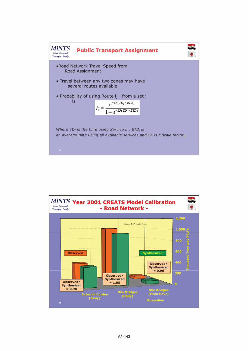
Public Transport AssignmentPublic Transport Assignment
•Road Network Travel Speed from Road Assignment
T l b t t h• Travel between any two zones may haveseveral routes available
• Probability of using Route i, from a set j is
Where TDi is the time using Service i. , ETDi isan average time using all available services and SF is a scale factor..
47
MiNTSMisr National
Transport Study
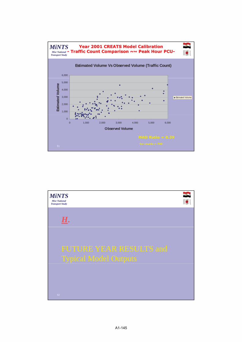
YearYear 2001 2001 CREATS Model CalibrationCREATS Model Calibration-- Road Network Road Network --
1,000
1,200
U's
Source: JICA Study Team.
400
600
800
Th
ou
san
d T
wo
-way P
CU
Observed Synthesized
Observed/ Synthesized
= 0 96
48
External Cordon(Daily)
Nile Bridges(Daily)
Nile Bridges(Peak Hour)
0
200
T
Screenline
Observed/ Synthesized
= 0.98
Observed/ Synthesized
= 1.08
= 0.96
A1-143

25
MiNTSMisr National
Transport Study
YearYear 2001 2001 CREATS Model CalibrationCREATS Model Calibration-- Public Transport Public Transport --
6.0
7.0
s
Source: JICA Study Team.
Synthesized
2.0
3.0
4.0
5.0
Millio
n D
aily B
oard
ing
s
Observed
y
Public Bus Shared Taxi Metro Other
0.0
1.0
Mode
Overall Public Transport System
Observed/Synthesized = 0.981
49
MiNTSMisr National
Transport Study
YearYear 2001 2001 CREATS Model CalibrationCREATS Model Calibration-- Traffic Count Comparison~~ DailyTraffic Count Comparison~~ Daily PCUPCU--
Estimated Volume vs Observed Volume (Traffic Count)
20 000
30,000
40,000
50,000
60,000
70,000
80,000
90,000
100,000
Ob
bse
rve
d V
olu
me
Estimated Volume
0
10,000
20,000
0 10,000 20,000 30,000 40,000 50,000 60,000 70,000 80,000 90,000 100,000
Estimated Volume
O
MAD Ratio = 0.34
50
A1-144
26
MiNTSMisr National
Transport Study
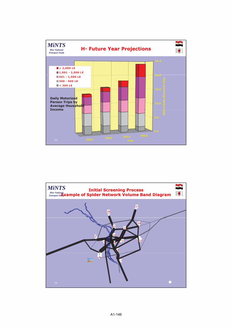
Year 2001 CREATS Model CalibrationYear 2001 CREATS Model Calibration-- Traffic Count ComparisonTraffic Count Comparison ~~ Peak Hour PCU~~ Peak Hour PCU--
Estimated Volume Vs Observed Volume (Traffic Count)
6,000
1,000
2,000
3,000
4,000
5,000
Est
imate
d V
olu
me
Estimated Volume
MAD Ratio = 0.39
for counts > 700
0
0 1,000 2,000 3,000 4,000 5,000 6,000
Observed Volume
51
MiNTSMisr National
Transport Study
H.
FUTURE YEAR RESULTS and Typical Model Outputs
52
A1-145
27
MiNTSMisr National
Transport Study
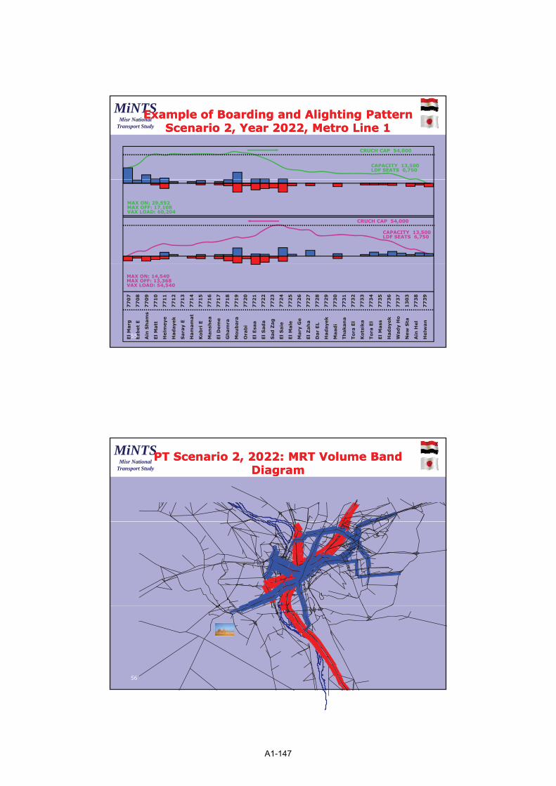
HH-- Future Year ProjectionsFuture Year Projections
20 0
25.0
> 2,000 LE
1,001 - 2,000 LE
10.0
15.0
20.0
ion
Dail
y M
oto
rize
d T
rip
s501 - 1,000 LE
300 - 500 LE
< 300 LE
Daily Motorized Person Trips byAverage Household Income
2001 2007 2012 2022
0.0
5.0
Mil
li
Year
Income
53
MiNTSMisr National
Transport Study
Initial Screening ProcessInitial Screening ProcessExample of Spider Network Volume Band DiagramExample of Spider Network Volume Band Diagram
16
17
2
3
8
9
10
11 12
13
1415
47
54
A1-146
28
MiNTSMisr National
Transport Study
Example of Boarding and Alighting PatternExample of Boarding and Alighting PatternScenarioScenario 22, Year , Year 20222022, Metro Line , Metro Line 11
CAPACITY 13,500LDF SEATS 0,750
CRUCH CAP 54,000
MAX ON: 29,552MAX OFF: 17,108VAX LOAD: 60,204
CAPACITY 13,500LDF SEATS 6,750
CRUCH CAP 54,000
El M
arg
Ezb
et
E
Ain
Sh
am
s
El M
att
Helm
eye
Had
ayek
Sara
y E
Ham
am
at
Ko
bri
E
Man
shea
El D
em
e
Gh
am
ra
Mo
ub
ara
Ora
bi
El E
saa
El S
ad
a
Sad
Zag
El S
aie
El M
ale
Mary
Ge
El Z
ah
a
Dar
EL
Had
ayek
Maad
i
Th
akan
a
To
ra E
l
Ko
tsik
a
To
ra E
l
El M
ass
Had
ayek
Wad
y H
o
New
Sta
Ain
Hel
Helw
an
77
07
77
08
77
09
77
10
77
11
77
12
77
13
77
14
77
15
77
16
77
17
77
18
77
19
77
20
77
21
77
22
77
23
77
24
77
25
77
26
77
27
77
28
77
29
77
30
77
31
77
32
77
33
77
34
77
35
77
36
77
37
13
03
77
38
77
39
MAX ON: 14,540MAX OFF: 13,368VAX LOAD: 54,540
55
MiNTSMisr National
Transport Study
PT Scenario PT Scenario 22,, 20222022: MRT Volume Band : MRT Volume Band DiagramDiagram
56
A1-147

29
MiNTSMisr National
Transport Study
Trip Generation ResultsTrip Generation Results
Year Household Income(’01 LE)
Total MechanisedTrips(Mil)
Trips in Class 4 and 5
Trips per HH
(Mil)
2001 672 14.4 3.7 4.11
2012 879 19.2 7.2 4.65
57
2022 1,176 25.1 12.7 4.94
MiNTSMisr National
Transport Study
AverageAverage Personal Travel Speed Personal Travel Speed SpeedSpeed
Scenario Person Speed Index
Base Year 2001 100
Do Minimum 2022 64
Master Plan Network in2022
95
36 % Decrease
50 % Increase
58
2022
A1-148
30
MiNTSMisr National
Transport Study
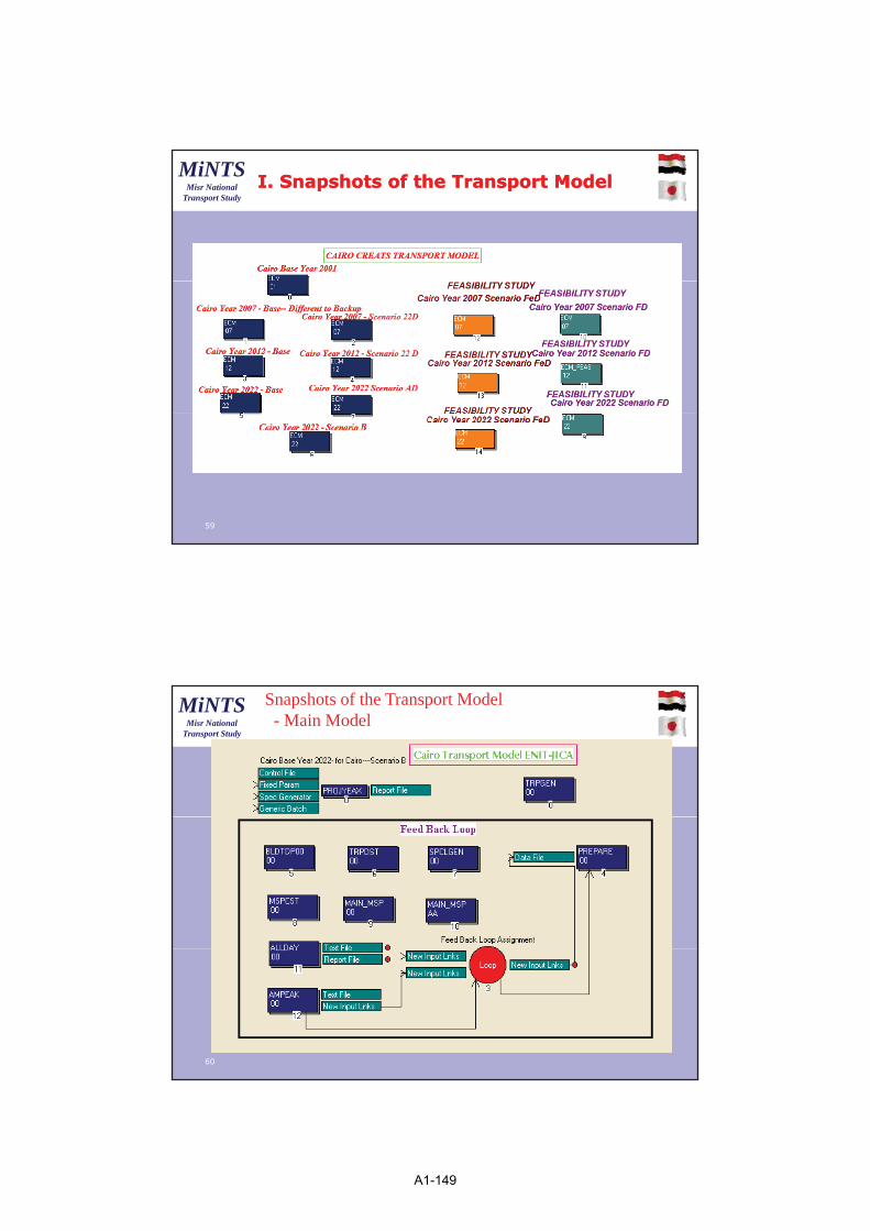
I. Snapshots of the Transport ModelI. Snapshots of the Transport Model
59
MiNTSMisr National
Transport Study
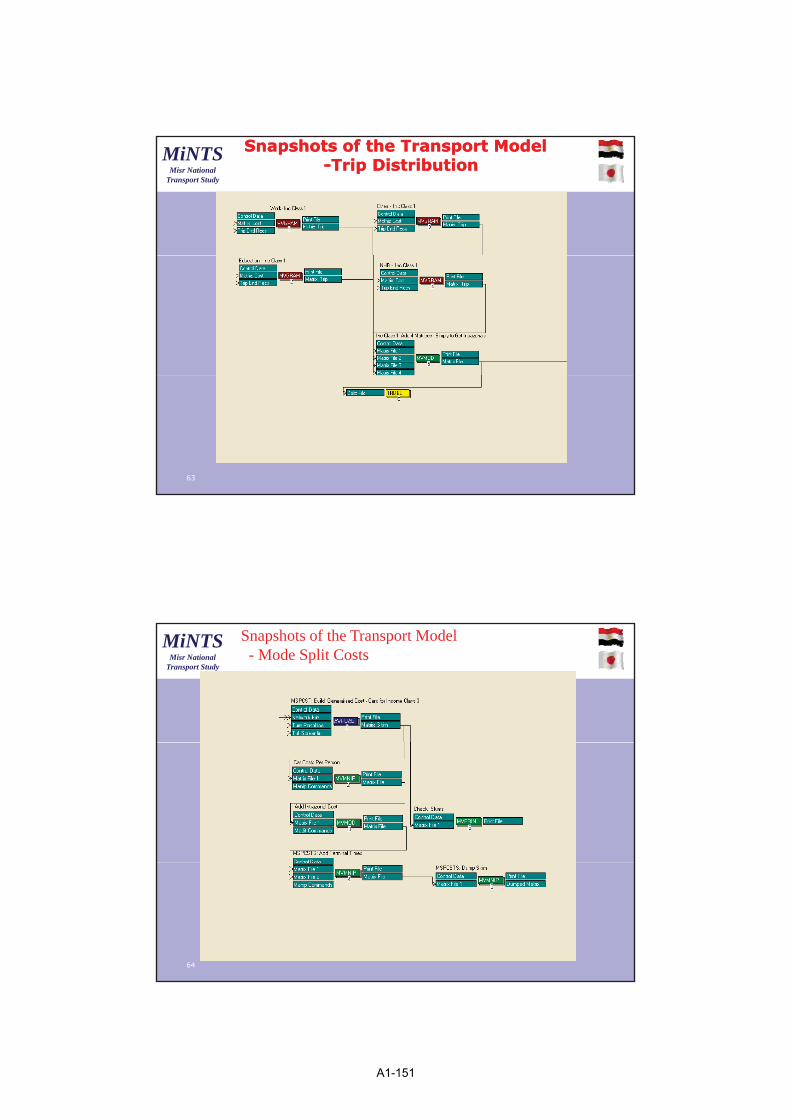
Snapshots of the Transport Model - Main Model
60
A1-149

31
MiNTSMisr National
Transport Study
61
MiNTSMisr National
Transport Study
Snapshots of the Transport Model Snapshots of the Transport Model --Trip GenerationTrip Generation
62
A1-150
32
MiNTSMisr National
Transport Study
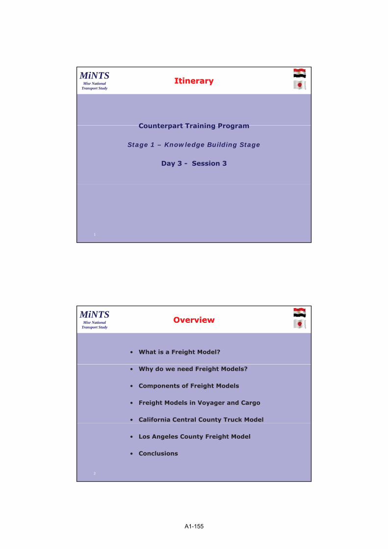
Snapshots of the Transport Model Snapshots of the Transport Model --Trip DistributionTrip Distribution
63
MiNTSMisr National
Transport Study
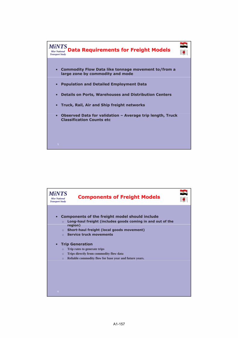
Snapshots of the Transport Model - Mode Split Costs
64
A1-151

33
MiNTSMisr National
Transport Study
Snapshots of the Transport Model Snapshots of the Transport Model --Modal splitModal split
65
MiNTSMisr National
Transport Study
Snapshots of the Transport Model Snapshots of the Transport Model -- Daily Trip TableDaily Trip Table
66
A1-152

34
MiNTSMisr National
Transport Study
Future Average Household IncomeFuture Average Household Income
Year 2001---- 672 (’01 LE per Month)
Year 2007 ---- 754 (’01 LE per Month)
Year 2012---- 879 (’01 LE per Month)
Year 2022--1,176 (’01 LE per Month)
67
MiNTSMisr National
Transport Study
Future Average Household IncomeFuture Average Household Income
Year 2001---- 672 (’01 LE per Month)
Year 2007 754 (’01 LE per Month)Year 2007---- 754 ( 01 LE per Month)
Year 2012---- 879 (’01 LE per Month)
Year 2022---- 1,176 (’01 LE per Month)(E i 2022 th l 16 ith(Even in 2022, there are only 16 zones with
income greater than 3,000 LE per Month)
68
A1-153

35
MiNTSMisr National
Transport Study
AA-- Zoning System and NetworkZoning System and Network
ZONING SYSTEM
--- For Cairo Transport Model, based on some Combined Shiakhas - 464 Internal Zones and 19 External Stations
69
A1-154
1
MiNTSMisr National
Transport Study
ItineraryItinerary
Counterpart Training ProgramCounterpart Training Program
Stage 1 – Knowledge Building Stage
Day 3 - Session 3
1
MiNTSMisr National
Transport Study
OverviewOverview
• What is a Freight Model?
• Why do we need Freight Models?
• Components of Freight Models
• Freight Models in Voyager and Cargo
• California Central County Truck Model
2
• Los Angeles County Freight Model
• Conclusions
A1-155

2
MiNTSMisr National
Transport Study
What is a Freight Model?What is a Freight Model?
• A tool to model the movement of goods in a region
• Goods (in tons) movement can then be split into modes (trucks, rail, air, ship)
• Example: 300 tons of timber is moving from A to B by truck. Each truck can carry 3 tons – translates to 100 trucks
3
MiNTSMisr National
Transport Study
Why develop separate Freight ModelsWhy develop separate Freight Models
• Significant growth in goods movement require improved models to evaluate impacts on roadway capacity and air
litquality
• Models needed to address different potential improvements
o Higher capacity intermodal rail terminalso Truck-only laneso Extended working hours at the portso Short-haul shuttles from ports to inland freight facilities
4
o Short haul shuttles from ports to inland freight facilities
A1-156
3
MiNTSMisr National
Transport Study
Data Requirements for Freight ModelsData Requirements for Freight Models
• Commodity Flow Data like tonnage movement to/from a large zone by commodity and mode
• Population and Detailed Employment Data
• Details on Ports, Warehouses and Distribution Centers
• Truck, Rail, Air and Ship freight networks
5
• Observed Data for validation – Average trip length, Truck Classification Counts etc
MiNTSMisr National
Transport Study
Components of Freight ModelsComponents of Freight Models
• Components of the freight model should includeo Long-haul freight (includes goods coming in and out of the
i )region)o Short-haul freight (local goods movement)o Service truck movements
• Trip Generationo Trip rates to generate trips
o Trips directly from commodity flow data
o Reliable commodity flow for base year and future years.
6
A1-157

4
MiNTSMisr National
Transport Study
Components of Freight ModelsComponents of Freight Models
• Trip Distributiono Directly from commodity flow datao Gravity Model / Modified Gravity Model
• Mode Choice Modelo Directly from commodity flow datao Estimated Mode Choice Model
• Trip Assignment / Trip Chaining
7
• Forecasts should recognize trends in labor productivity, imports, and exports
MiNTSMisr National
Transport Study
Freight Models in Voyager and CargoFreight Models in Voyager and Cargo
Central California Voyager Model with linkages to remainder of USA
L H l F i h di l
Los Angeles County Cargo Model
T l F i h i d• Long Haul Freight directlyfrom Commodity Flow Data (CFD)
• Short Haul Freight from trip generation model
• Long Haul freight
• Total Freight estimatedfrom trip generation model
• Trip rates for long and short haul freight estimated from CFD
Long Haul freight distribution directly from CFD, Short Haul by gravity model
• Freight distribution done by a joint distribution-mode choice model.
8
A1-158

5
MiNTSMisr National
Transport Study
Freight Models in Voyager and CargoFreight Models in Voyager and Cargo
Central California Voyager Model with linkages to remainder of USA
N M d Ch i
Los Angeles County Cargo Model
M l i i l L i M d• No Mode Choice
• No trip chaining
• Multi – class assignment
• Forecasts using growth factors
• Multinomial Logit - ModeChoice
• Trip Chaining represented in the TLN Model
• Forecasts use changes in productivity and trends in imports / exports
factorsp p
9
MiNTSMisr National
Transport Study
Trip Generation ModelsTrip Generation Models––Central CaliforniaCentral California
• Based on County Level Commodity Flow Data (Data on tonnage of goods from place to place.
• Convert County Level CFD to TAZ level
• Model structure is based on two overlapping elementso Intercity trips estimated using ITMS commodity flow data and
local employment datao Local truck trips estimated based on a combination of land use,
employment, and special generator data
10
p y , p g
A1-159
6
MiNTSMisr National
Transport Study
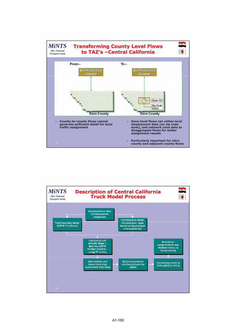
Transforming County Level Flows Transforming County Level Flows to TAZ’s to TAZ’s ––Central CaliforniaCentral California
11
o County-to-county flows cannotgenerate sufficient detail for local traffic assignment
o Zone-level flows can utilize local employment data (on zip code level), and network zone data to disaggregate flows for better assignment results
o Particularly important for intra county and adjacent county flows
MiNTSMisr National
Transport Study
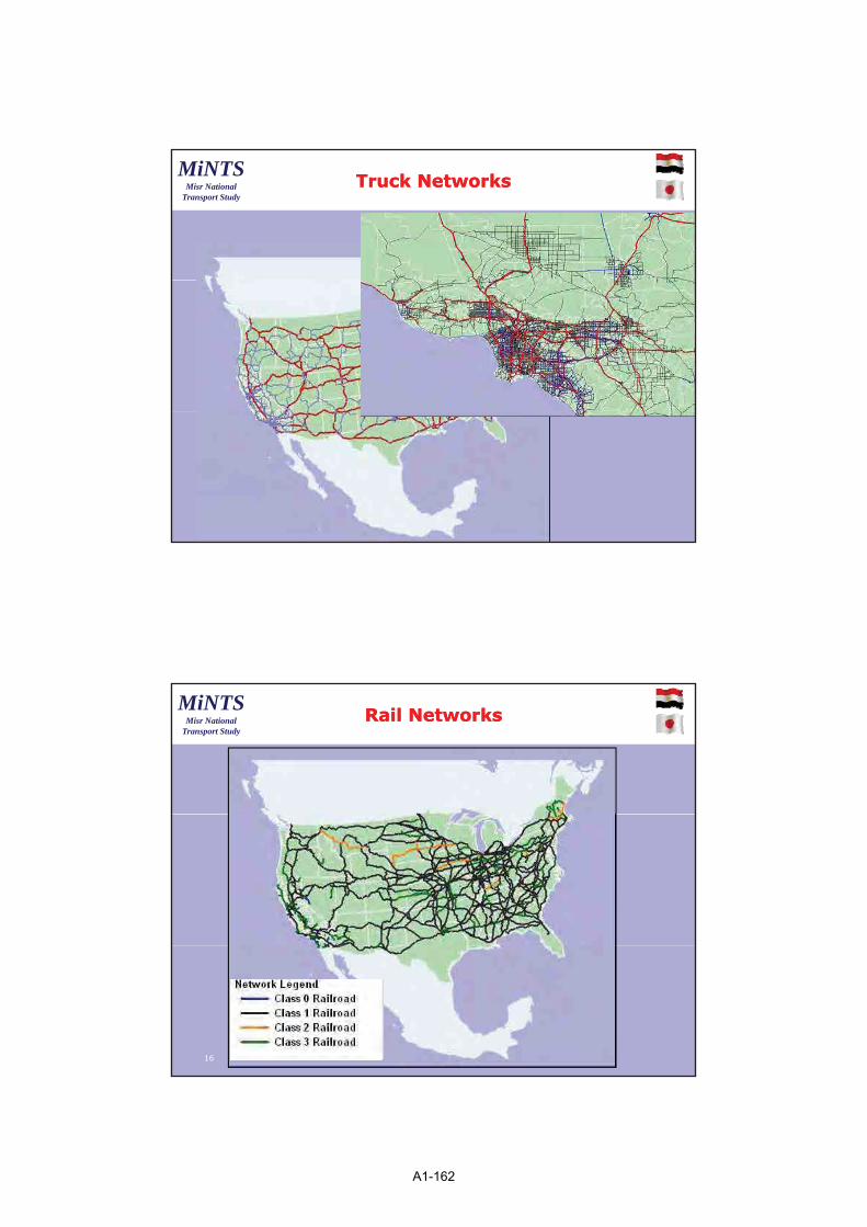
Description of Central California Description of Central California TruckTruck Model ProcessModel Process
12
A1-160

7
MiNTSMisr National
Transport Study
Los Angeles Cargo Modeling ProcessLos Angeles Cargo Modeling Process
13
MiNTSMisr National
Transport Study
Study AreaStudy Area
• Within 5 county SCAG region – zip codes
• Remainder of California – counties
• Remainder of USA – states
• 4 external zones; 2 each forCanada and Mexico
14
A1-161
8
MiNTSMisr National
Transport Study
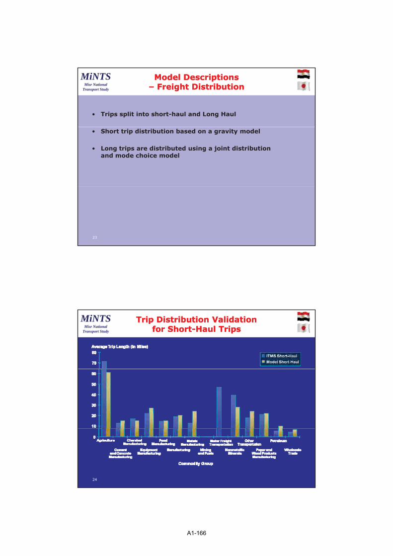
Truck NetworksTruck Networks
15
MiNTSMisr National
Transport Study
Rail NetworksRail Networks
16
A1-162

9
MiNTSMisr National
Transport Study
Truck Time FunctionsTruck Time Functions
• LTL Time = Time+40 hrs for loading / unloading
• TL Times – Drive 11 hrs between rest periods of 10 hrs
17
MiNTSMisr National
Transport Study
Truck Cost FunctionsTruck Cost Functions
Costs are based on labor and fuel costs:
• LTL Costso 500 to 1,000 mile trips - $1.80 to $2.30 per mileo > 1000 mile trips - $1.75 to $2.00 per mile
• TL Costso 500 to 1,000 mile trips - $1.35 to $1.74 per mileo > 1,000 miles trips - $1.32 to $1.51 per mile
18
A1-163

10
MiNTSMisr National
Transport Study
Rail Time ad Cost FunctionsRail Time ad Cost Functions
• Average rail speed of 33mph and 24hrs terminal / dray time
I t d l t il hi t @ 14 t / it $26 43/t• Intermodal trailer shipments @ 14 tons/unit: = $26.43/ton +$.05/ton-mile;
• Intermodal container shipments @ 16 tons/unit: = $23.13/ton + $.04/ton-mile; and
19
MiNTSMisr National
Transport Study
Model Descriptions Model Descriptions –– Freight GenerationFreight Generation
• Forecasts annual tons by commodity
• Implemented at the Coarse Zone Level
• Internal tonnage based on tonnage rate per employee
• Consumptions based on Input-Output matrix
• I-E and E-I trips allocated based on factors derived
20
from ITMS
• Port trips added directly from the Port’s models
A1-164

11
MiNTSMisr National
Transport Study
Tonnage Rates by CommodityTonnage Rates by Commodity
Category Description Tonnage Rate
Crops 311.51
Livestock 4 863 69Agriculture
Livestock 4,863.69
Forestry, fishing, hunting, and trapping 7,329.10
Cement and Concrete Manufacturing
Stone, clay, glass products 472.50
Concrete products 7,502.27
Chemical Manufacturing Chemicals and allied products 488.26
Equipment Manufacturing
Industrial machinery and equipment 36.83
Electrical and electronic equipment 36.60
Transportation Equipment 72.96
Textile mill products 200.58
21
Manufactuing
Apparel and other textile products 8.15
Furniture and fixtures 49.60
Printing and publishing 24.47
Rubber and miscellaneous plastics 170.78
Leather and leather products 412.91
Instruments and related products 1.84
Miscellaneous manufacturing industries 7.86
MiNTSMisr National
Transport Study
Tonnage Rates by CommodityTonnage Rates by Commodity(contd.)(contd.)
Category Description Tonnage Rate
Metals Manufacturing Primary metal industries 816.73
Fabricated metal products 101.65
Mining and Fuels Mining and oil and gas 5,123.91
Motor Freight Transportation Motor freight transportation and warehousing 512.42
Nonmetallic Minerals Nonmetallic minerals, except fuels 45,695.22
Other Transportation
Transportation by air 802.89
Transportation services 562.11
Paper and Wood Products Manufacturing
Lumber and wood products 763.23
22
ManufacturingPaper and allied products 243.28
Petroleum Petroleum and coal products 7,506.25
Wholesale Trade Wholesale trade – durable goods 62.57
A1-165
12
MiNTSMisr National
Transport Study
Model Descriptions Model Descriptions –– Freight DistributionFreight Distribution
• Trips split into short-haul and Long Haul
• Short trip distribution based on a gravity model
• Long trips are distributed using a joint distribution and mode choice model
23
MiNTSMisr National
Transport Study
Trip Distribution Validation Trip Distribution Validation for Shortfor Short--Haul TripsHaul Trips
24
A1-166

13
MiNTSMisr National
Transport Study
Model DescriptionsModel Descriptions
• Mode Choiceo Estimates Truck and Rail Trips o Based on a multinomial logit modelo Applied for 3 distance classes
• Service Modelo Estimates safety, utility, public / personal vehicles
• Fine Distribution Modelo Disaggregates trips from coarse zone level to the fine-
25
o Disaggregates trips from coarse zone level to the finezone system
MiNTSMisr National
Transport Study
Vehicle ModelVehicle Model
• Converts tons to trucks
• Parameters to influence empty trucks
• Standard Vehicle Model to generate direct O-D flows
• Touring vehicle model that simulates multi-point pick-up and drop off
26
A1-167

14
MiNTSMisr National
Transport Study
Assignment ValidationAssignment Validation–– External CordonsExternal Cordons
Gateway Routes Count Volumes
Truck Model Volumes
%Difference
San Diego / Mexico
I-8, I-15, I-5 26,058 24,436 -6%
Rest of CA US-101, I-5, CA-14, US-395
29,698 31,840 7%
Arizona I-8, I-15, I- 25,534 27,133 6%
27
, ,40, I-10
, ,
Total 81,291 83,409 3%
MiNTSMisr National
Transport Study
Assignment Validation Assignment Validation –– ScreenlinesScreenlines
Screenline Dir Number of Counts
Truck Counts
Model Volumes
% Diff
1 N-S 18 51,277 54,718 7%
2 E-W 28 96,480 91,096 -6%, ,
3 N-S 18 70,323 53,375 -24%
4 E-W 12 71,266 56,140 -21%
5 E-W 23 77,268 74,714 -3%
6 E-W 13 78,972 86,753 10%
7 N-S 20 47,733 25,909 -46%
8 E-W 14 64,199 60,048 -6%
10 E-W 8 19,356 20,397 5%
28
11 E-W 8 16,278 18,389 13%
12 E-W 5 19,064 18,617 -2%
13 N-S 6 17,291 14,349 -17%
18 N-S 4 29,958 31,331 5%
Total 191 700,699 644,421 -8%
A1-168

15
MiNTSMisr National
Transport Study
2030 Model 2030 Model –– Tonnage Generation ModelTonnage Generation ModelChange in Labor ProductivityChange in Labor Productivity
Commodity Group Growth
Agriculture 1.43%
Cement and Concrete 0.66%
Chemical Manufacturing 1.85%
Equipment Manufacturing 2.55%
Food Manufacturing 1.47%
Manufacturing 3.39%
Metals Manufacturing 2.12%
Mining and Fuels 0.93%
Motor freight transportation 1 18%
29
Motor freight transportation 1.18%
Nonmetallic minerals 1.88%
Other transportation 1.93%
Paper and Wood Products 1.71%
Petroleum 2.57%
Wholesale Trade 3.94%
MiNTSMisr National
Transport Study
2030 Model 2030 Model –– Tonnage Generation Tonnage Generation ModelChangeModelChange in Imports and Exportsin Imports and Exports
Region / State Exports Imports
Remainder of CA -8% -1%
Sacramento -1% 0%
San Francisco Bay Area -4% 0%San Francisco Bay Area 4% 0%
San Diego -2% 4%
Florida 1% 0%
Illinois 1% 0%
Iowa 0% -1%
Arkansas 0% -1%
Texas 2% -2%
Colorado 0% 2%
30
Arizona 1% 7%
Utah 1% 0%
Nevada 2% -3%
Washington 1% -2%
Oregon 1% 0%
Mexico 0% 2%
A1-169
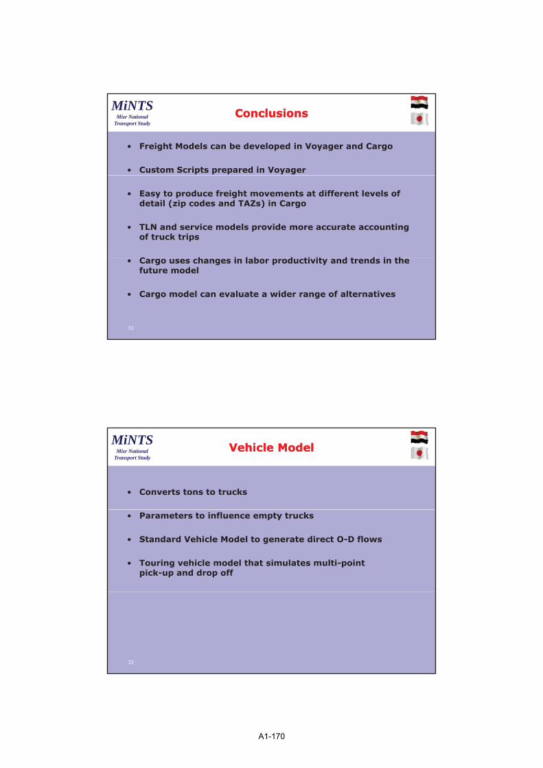
16
MiNTSMisr National
Transport Study
ConclusionsConclusions
• Freight Models can be developed in Voyager and Cargo
• Custom Scripts prepared in Voyager
• Easy to produce freight movements at different levels of detail (zip codes and TAZs) in Cargo
• TLN and service models provide more accurate accounting of truck trips
C h i l b d i i d d i h
31
• Cargo uses changes in labor productivity and trends in thefuture model
• Cargo model can evaluate a wider range of alternatives
MiNTSMisr National
Transport Study
Vehicle ModelVehicle Model
• Converts tons to trucks
• Parameters to influence empty trucks
• Standard Vehicle Model to generate direct O-D flows
• Touring vehicle model that simulates multi-point pick-up and drop off
32
A1-170

1
MiNTSMisr National
Transport Study
ItineraryItinerary
Counterpart Training ProgramCounterpart Training Program
Stage 1 – Knowledge Building Stage
Day 4 - Session 1
1
MiNTSMisr National
Transport Study
The ModelThe Model
Roots in transportation economics and theory of supply / demand equilibrium
Transportation supply = The Network --- roads, bridges, trains, buses airports boats planesbuses, airports, boats, planes
Transportation demand – the demand for activities (goods & services) and Travel
Transportation costs = expected time, distance, money, and other penalties associated with using a travel option
Weighted combination of these costs is called �generalized cost
Costs increase with demand -congestion
Demand on a Mode or Route decreases with cost –diversion
2
A1-171
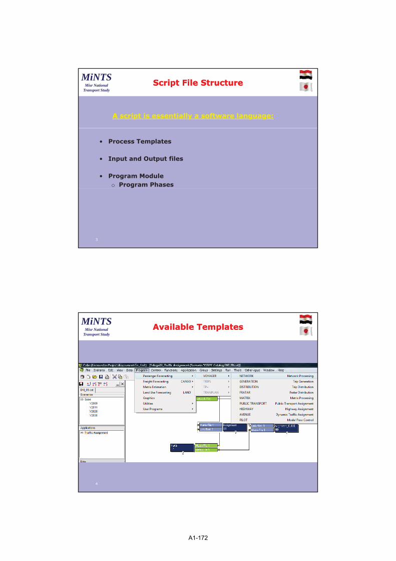
2
MiNTSMisr National
Transport Study
Script File StructureScript File Structure
A script is essentially a software language:
• Process Templates
• Input and Output files
• Program Moduleo Program Phases
3
MiNTSMisr National
Transport Study
Available TemplatesAvailable Templates
4
A1-172

3
MiNTSMisr National
Transport Study
Sample TemplatesSample Templates
5
MiNTSMisr National
Transport Study
Demand Data used in the ModelDemand Data used in the Model
• Zonal Datao Stores socio-economic & demographic information,
trip endso Exchange formats: ASCII (e.g. CSV) text, DBF (SHP)o Exchange formats: ASCII (e.g. CSV) text, DBF (SHP)o Best GIS format: geodatabase polygon feature class
• Matrix Datao Zone-to-zone information of any kind e.g. trips,
costso Native binary MAT format for compression,
efficiencyo ASCII (e.g. CSV) text, DBF formats for exchange( g ) g
• Record and Database Fileso ASCII (e.g. CSV) text, DBF, MS Access 2003, ESRI
personal geodatabase formats
• Lookup Tableso ASCII (e.g. CSV) text, DBF formats
6
A1-173

4
MiNTSMisr National
Transport Study
Supply Data used in the ModelSupply Data used in the Model
• Highway� networkso Native binary Citilabs format for compression & efficiencyo ESRI custom personal geodatabasefeature dataset for GISo ASCII (CSV) text and DBF for exchangeo ASCII (CSV) text and DBF for exchange
• Intersection / junction datao ASCII text format (Cube Voyager syntax)o Roundabout, priority, fixed-time and adaptive signals, two-
way and all-way stopso Used to apply HCM 2000 or saturation flow lane group
capacity and delay
• Public transport servicesu c a spo se ceso ASCII text format (Cube Voyager syntax): lines, system
data, fares, factorso Binary format to consolidate data with underlying
multimodal networko ESRI personal geodatabaseformat: lines, non-transit legs
7
MiNTSMisr National
Transport Study
CUBE Voyager Syntax and StructureCUBE Voyager Syntax and Structure
• All statements follow the same general structure: COMMANDKEYWORD=VALUE, SUBKEYWORD = VALUESome KEYWORDs automatically invoke an associated• Some KEYWORDs automatically invoke an associated COMMAND
• KEYWORDs are always followed by an equals sign and a VALUE
• The VALUE may be the result of an expression or computation
• Continuation characters (commas, equals signs, any t ) di t ib t t t t lti l lioperator) distribute statements across multiple lines
• E.g.: COMMAND,KEYWORD=VALUE,SUBKEYWORD=VALUE
8
A1-174

5
MiNTSMisr National
Transport Study
Voyager ExpressionsVoyager Expressions
• Operators:+ addition || logical OR
- subtraction &&logical AND* lti li ti l* multiplication ==, =equals/ division !=, <>does not equal% modulus >=greater than or equal to^ exponentiation <=less than or equal to
() parentheses >greater than<less than
• Numeric functions: ABS, INT, ROUND, MAX, MINEXP, LN, LOG, POW, SQRTRAND, RANDOM, RANDSEEDQ
• Character Functions
DELETESTR(s1,n1,n2), DUPSTR(str,n), FORMAT(x,w,d,str), INSERTSTR(s1,s2,n),LEFTSTR(s1,n), LTRIM(str), REPLACESTR(s1,s2,s3,n), REPLACESTRIC(s1,s2,s3,n), REVERSESTR(s1),RIGHTSTR(s1,n), STR(v,w,d), STRLEN(str), STRLOWER(str), STRPOS(str,str2),STRPOSEX(s1,s2,n1), STRUPPER(str), SUBSTR(str,b,n), TRIM(str), VAL(str)
9
MiNTSMisr National
Transport Study
Commands used in all ModesCommands used in all Modes
• COMP var= expression; usually without explicit COMP
• IF (condition)… ELSEIF (condition)… ELSE… ENDIF
• LOOP… ENDLOOP
• LOOKUP
• PRINT LIST= a, b, c; where a, b, and c are variables or expressionsexpressions
o FORM = w.d; where w is the default width and d is the number of decimalso FILE = filename or PRINTO=#o CSV = T; automatically format as comma-separated values
10
A1-175

6
MiNTSMisr National
Transport Study
Comments and Style GuidelinesComments and Style Guidelines
• Include plenty of comments—for yourself and others• Everything following a semi-colon on any line is a comment• Use ; comments to explain intent behind coded commands
o Everything between /* and */ is a control blocko Everything between / and / is a control block o Use control blocks to turn off sections of script without deleting
• Use full COMMAND KEYWORD=VALUE syntax when possible• Write system commands, keywords, and functions in
UPPERCASE, reserve lower and proper case for user-defined variables and names
• NEVER have your script file open when you are linking new files into a Voyager Module Input and output files will notfiles into a Voyager Module. Input and output files will not get updated!
• Try right-clicking when you are unsure what should come next
11
MiNTSMisr National
Transport Study
Program Module StructureProgram Module Structure
• Cube Voyager program modules may contain one or more “phases”
• Each phase performs a user-specified sequence of operations on each element of a data structure, such as p ,links in a network
• Typical program script:;Comments preceded by semicolonRUN PGM=nameFILEI … ;specify input filesFILEO … ;specify output filesPARAMETERS … ;global settings not in any phasePROCESS PHASE=…
Note: The Colours1. Green is a comment2. Red is the beginning and ending of a program
COMMAND KEYWORD=…;more commands…
ENDPROCESS;more phases…
ENDRUN• Additionally, some programs have an iterative looping
framework that will repeat certain phases until a convergence criterion is met12
A1-176

7
MiNTSMisr National
Transport Study
Sample Script File from a Process TemplateSample Script File from a Process Template
;;<<PROCESS TEMPLATE>><<MATRIX>>;;;{note1,note,12,"Perform basic mathematical operations on 2 tables"} >>>;{note2,note,10,"The script will operate on the first table of each file"} >>>;{note3,note,8,"Example: mi.1.table1 + mi.2.table1"} >>>;Input Matrix File 1: {mati1,filename,"Enter Input Trip Matrix 1",x,"","Trip Matrix (*.mat)|*.mat"};Input Matrix File 2: {mati2,filename,"Enter Input Trip Matrix 2",x,"","Trip Matrix (*.mat)|*.mat"};Output Matrix File: {mato,filename,"Enter Output Matrix File Name",x,"","Matrix File (*.mat)|*.mat"};Mathematical Operator: {operator,RadioBtn,"Chose Operation","*","/","-","+"};*******************************************************************; BASIC MATHEMATICS * ;*******************************************************************; BY CITILABS;; THIS SCRIPT READS TWO TRIP MATRICES, CREATES A MATRIX WITH THE RESULT;;<<End Parameters>>;;
; Do not change filenames or add or remove FILEI/FILEO statements using an editor. Use Cube/Application Manager.
RUN PGM=MATRIXFILEI MATI[1] = {MATI1.Q} FILEI MATI[2] = {MATI2.Q}
FILEO MATO[1] = {MATO Q}FILEO MATO[1] {MATO.Q}, MO=10
MW[1]=mi.1.1 MW[2]=mi.2.1
if ('{operator}'<>'/') MW[10]=MW[1]{operator}MW[2]
else JLOOP if (MW[2]<>0) MW[10]=MW[1]{operator}MW[2] ENDJLOOP ENDIF
ENDRUN13
MiNTSMisr National
Transport Study
Sample Script File from a Process TemplateSample Script File from a Process Template
;;<<PROCESS TEMPLATE>><<MATRIX>>;;;{note1,note,12,"Perform basic mathematical operations on 2 tables"} >>>;{note2,note,10,"The script will operate on the first table of each file"} >>>;{note3,note,8,"Example: mi.1.table1 + mi.2.table1"} >>>;Input Matrix File 1: {mati1,filename,"Enter Input Trip Matrix 1",x,"","Trip Matrix (*.mat)|*.mat"};Input Matrix File 2: {mati2,filename,"Enter Input Trip Matrix 2",x,"","Trip Matrix (*.mat)|*.mat"};Output Matrix File: {mato,filename,"Enter Output Matrix File
Allows inclusion of specific input menu
Name",x,"","Matrix File (*.mat)|*.mat"};Mathematical Operator: {operator,RadioBtn,"Chose Operation","*","/","-","+"};*******************************************************************; BASIC MATHEMATICS * ;*******************************************************************; BY CITILABS;; THIS SCRIPT READS TWO TRIP MATRICES, CREATES A MATRIX WITH THE RESULT;;<<End Parameters>>;;
; Do not change filenames or add or remove FILEI/FILEO statements using an editor. Use Cube/Application Manager.
RUN PGM=MATRIXFILEI MATI[1] = {MATI1.Q} FILEI MATI[2] = {MATI2.Q}
FILEO MATO[1] = {MATO Q}FILEO MATO[1] {MATO.Q}, MO=10
MW[1]=mi.1.1 MW[2]=mi.2.1
if ('{operator}'<>'/') MW[10]=MW[1]{operator}MW[2]
else JLOOP if (MW[2]<>0) MW[10]=MW[1]{operator}MW[2] ENDJLOOP ENDIF
ENDRUN14
A1-177
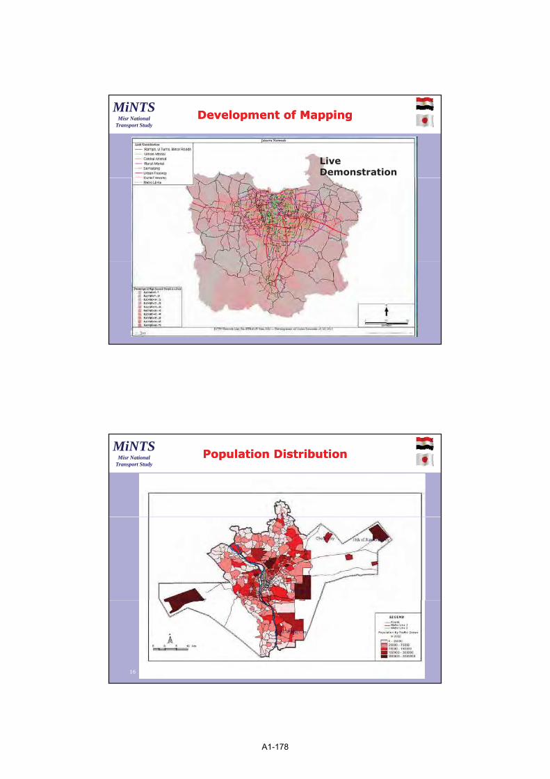
8
MiNTSMisr National
Transport Study
Development of MappingDevelopment of Mapping
Live Demonstration
15
MiNTSMisr National
Transport Study
Population DistributionPopulation Distribution
16
A1-178
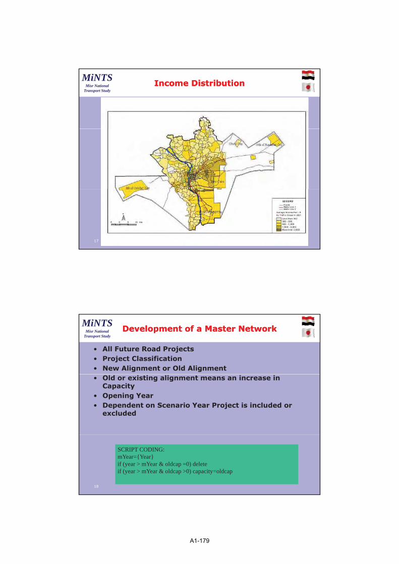
9
MiNTSMisr National
Transport Study
Income DistributionIncome Distribution
17
MiNTSMisr National
Transport Study
Development of a Master NetworkDevelopment of a Master Network
• All Future Road Projects• Project Classification• New Alignment or Old Alignment• Old or existing alignment means an increase in
Capacity• Opening Year• Dependent on Scenario Year Project is included or
excluded
SCRIPT CODING:mYear={Year}if (year > mYear & oldcap =0) deleteif (year > mYear & oldcap >0) capacity=oldcap
18
A1-179

1
MiNTSMisr National
Transport Study
ItineraryItinerary
Counterpart Training ProgramCounterpart Training Program
Stage 1 – Knowledge Building Stage
Day 4 - Sessions 2 and 3
1
MiNTSMisr National
Transport Study
A ModelA Model
Live Model Tour
2
A1-180
2
MiNTSMisr National
Transport Study
Building a Model from the BeginningBuilding a Model from the Beginning
• We will now build our first transport model
• Based on a Training Course developed by Citilabs
• We will only to do some of this today but you can finish in your own time, this is your homework.
•• WEWE SHOULD MEET ONE WEEK FROM NOW TO SEE IF SHOULD MEET ONE WEEK FROM NOW TO SEE IF YOU HAVE FINISHED THIS EXERCISE OR HAVE ANYYOU HAVE FINISHED THIS EXERCISE OR HAVE ANYYOU HAVE FINISHED THIS EXERCISE OR HAVE ANY YOU HAVE FINISHED THIS EXERCISE OR HAVE ANY PROBLEMS???PROBLEMS???
3
MiNTSMisr National
Transport Study
ApplicationsApplications
• The Applications are the Model Processes
A i l C t l h A li ti• A single Catalog may have many Applicationso Passenger Forecastingo Freight Forecastingo Land-Use Forecastingo Sub-Area Analysiso Impact Studies
• The Application file is a single page which tracks data flows and organizes modeling functions. These functions may be either from Cube Libraries or User Defined.
• Application files may be nested to provide model structure.
4
A1-181
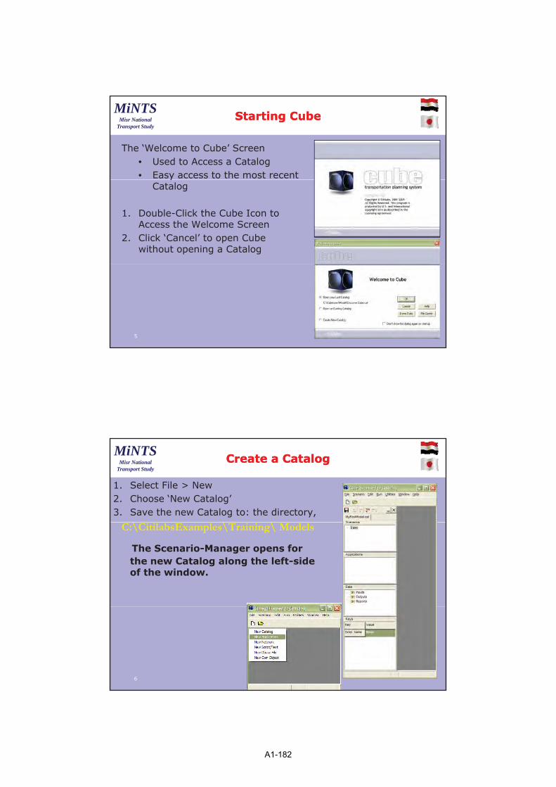
3
MiNTSMisr National
Transport Study
Starting CubeStarting Cube
The ‘Welcome to Cube’ Screen• Used to Access a Catalog• Easy access to the most recent y
Catalog
1. Double-Click the Cube Icon to Access the Welcome Screen
2. Click ‘Cancel’ to open Cube without opening a Catalog
5
MiNTSMisr National
Transport Study
Create a CatalogCreate a Catalog
1. Select File > New2. Choose ‘New Catalog’3. Save the new Catalog to: the directory,
C:\CitilabsExamples\Training\ Models
The Scenario-Manager opens for the new Catalog along the left-side of the window.
6
A1-182
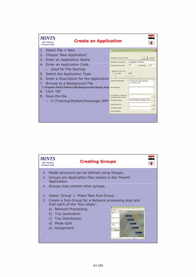
4
MiNTSMisr National
Transport Study
Create an ApplicationCreate an Application
1. Select File > New2. Choose ‘New Application’3. Enter an Application Name4 E A li i C d4. Enter an Application Code
– Used for File Naming5. Select the Application Type6. Enter a Description for the Application7. Browse to a Background FileCC::\\Program FilesProgram Files\\CitilabsCitilabs\\CubeCube\\BackgroundsBackgrounds\\citigrey.bmpcitigrey.bmp
8. Click ‘OK’9. Save the file
– C:\Training\Models\Passenger.APP
7
MiNTSMisr National
Transport Study
Creating GroupsCreating Groups
• Model structure can be defined using Groups.• Groups are Application files nested in the ‘Parent’
Application.• Groups may contain other groups.
1. Select ‘Group’ > ‘Make New Sub-Group…’2. Create a Sub-Group for a Network processing step and
then each of the ‘four-steps’.a) Network Processingb) Trip Generationb) Trip Generationc) Trip Distributiond) Mode Splite) Assignment
8
A1-183
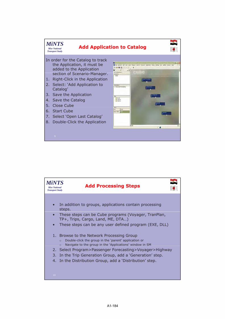
5
MiNTSMisr National
Transport Study
Add Application to CatalogAdd Application to Catalog
In order for the Catalog to track the Application, it must be added to the Application
ti f S i Msection of Scenario-Manager.1. Right-Click in the Application2. Select: ‘Add Application to
Catalog’3. Save the Application4. Save the Catalog5. Close Cube6. Start Cube 7. Select ‘Open Last Catalog’8. Double-Click the Application
9
MiNTSMisr National
Transport Study
Add Processing Steps Add Processing Steps
• In addition to groups, applications contain processing steps.
• These steps can be Cube programs (Voyager, TranPlan, TP+, Trips, Cargo, Land, ME, DTA…)
• These steps can be any user defined program (EXE, DLL)
1. Browse to the Network Processing Groupo Double-click the group in the ‘parent’ application oro Navigate to the group in the ‘Applications’ window in SMg g p pp
2. Select Program>Passenger Forecasting>Voyager>Highway3. In the Trip Generation Group, add a ‘Generation’ step.4. In the Distribution Group, add a ‘Distribution’ step.
10
A1-184
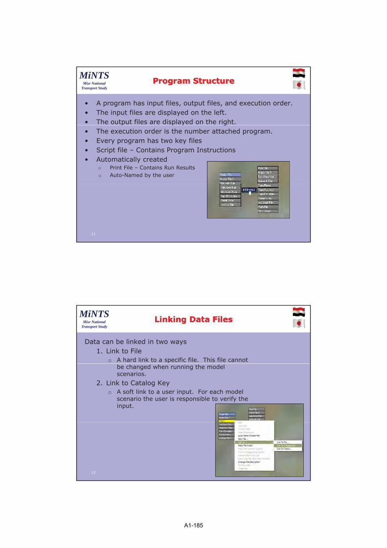
6
MiNTSMisr National
Transport Study
Program StructureProgram Structure
• A program has input files, output files, and execution order.• The input files are displayed on the left.• The output files are displayed on the right.p p y g• The execution order is the number attached program.• Every program has two key files• Script file – Contains Program Instructions• Automatically created
o Print File – Contains Run Resultso Auto-Named by the user
11
MiNTSMisr National
Transport Study
Linking Data FilesLinking Data Files
Data can be linked in two ways1. Link to File
o A hard link to a specific file. This file cannot be changed when running the model scenarios.
2. Link to Catalog Keyo A soft link to a user input. For each model
scenario the user is responsible to verify the input.
12
A1-185

7
MiNTSMisr National
Transport Study
Catalog KeysCatalog Keys
• Keys are the parameters that are input to the model which the developer would like the applier to be able to access and change.
• The values of the Keys are unique for each scenario and are tracked by the scenario manager.
• Keys may be numeric variables, file names, or text strings.
• The user accesses the keys through a user menu by double-clicking on a scenario.
• When the developer defines a key, they also define the user menu.
13
MiNTSMisr National
Transport Study
Creating a Catalog KeyCreating a Catalog Key
1. Right-click in the Keys window and select ‘Add’2. Enter a Name for the Key (Input Network)3. Enter a Prompt (Browse to the Input Network File)p ( p )4. Select the Type (File Name)5. Select the Control (Edit Box)6. Click on File Filters. Create a new filter.
o Enter a Filter Name: Networks (*.NET)o Enter a Filter: *.net
7. Click on AdvancedSele t ‘Sto e File Lo tion Rel ti e to C t log Di e to ’o Select ‘Store File Location Relative to Catalog Directory’
8. Click ‘OK’. The Key appears down in the Key window.9. Double-click on the ‘Base’ scenario to see the new
addition to the user interface.
14
A1-186
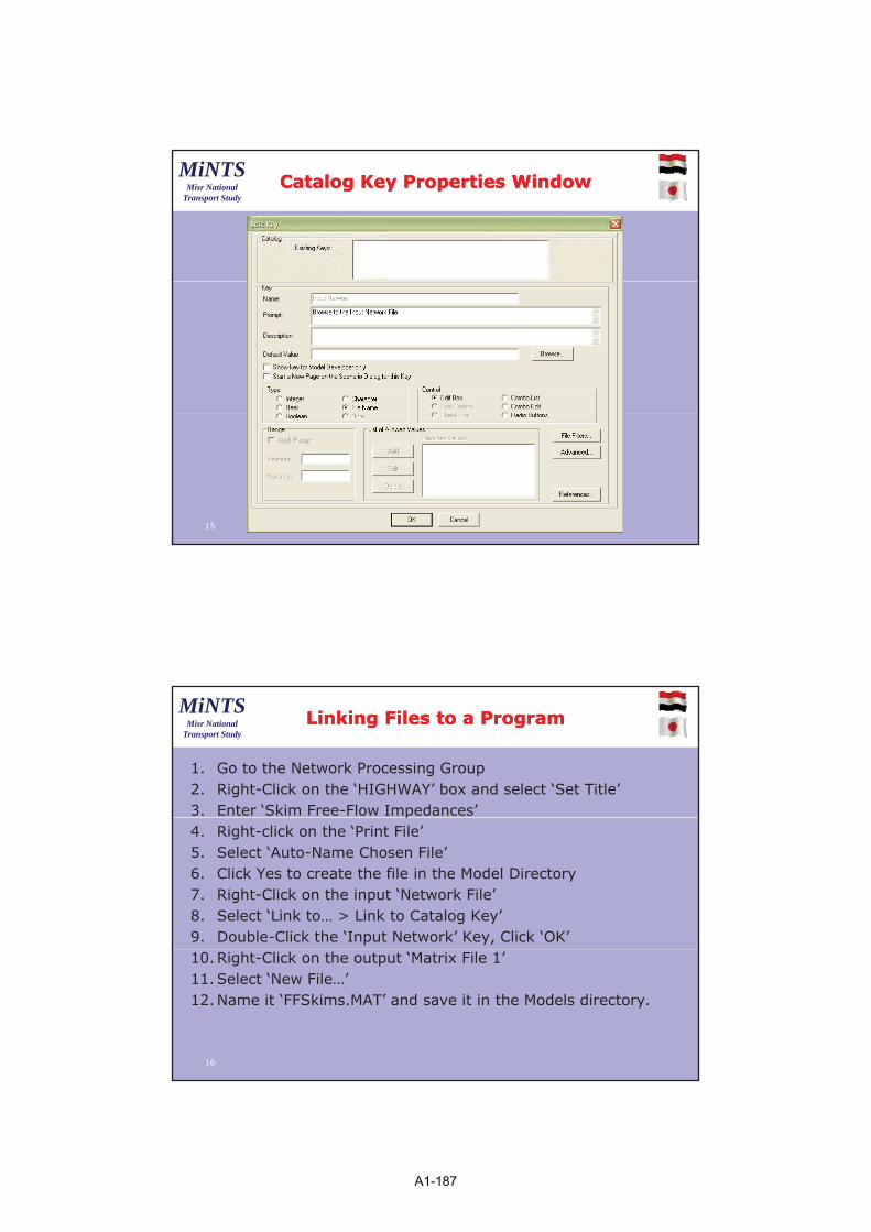
8
MiNTSMisr National
Transport Study
Catalog Key Properties WindowCatalog Key Properties Window
15
MiNTSMisr National
Transport Study
Linking Files to a ProgramLinking Files to a Program
1. Go to the Network Processing Group2. Right-Click on the ‘HIGHWAY’ box and select ‘Set Title’3. Enter ‘Skim Free-Flow Impedances’p4. Right-click on the ‘Print File’5. Select ‘Auto-Name Chosen File’6. Click Yes to create the file in the Model Directory7. Right-Click on the input ‘Network File’8. Select ‘Link to… > Link to Catalog Key’9. Double-Click the ‘Input Network’ Key, Click ‘OK’10.Right-Click on the output ‘Matrix File 1’ 11.Select ‘New File…’ 12.Name it ‘FFSkims.MAT’ and save it in the Models directory.
16
A1-187

9
MiNTSMisr National
Transport Study
Creating a Highway NetworkCreating a Highway Network
1. Open the Network Shape Fileo C:\Training\GISData\Network2005.shp\ g\ \ p
2. Select ‘GIS Tools > Build Network From Shape…’3. Save the new network as ‘Network2005.net’ in the
scenario folder ‘Base’.4. Select the A-Node and B-Node Field Name (A, B)5. For 1-way/2-way, use indicator field (ONEWAY_TWO)6. Do not add distance field
d l ( )7. Set Node grouping limit (1)8. Set Starting New Node Number (2000)9. Set Highest Zone Number (25)10.Click OK
17
MiNTSMisr National
Transport Study
Build Network DialogBuild Network Dialog
18
A1-188
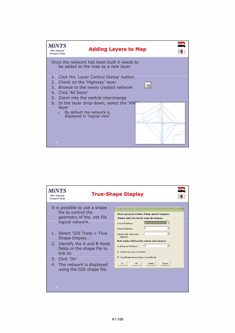
10
MiNTSMisr National
Transport Study
Once the network has been built it needs to be added to the map as a new layer.
1 Cli k th ‘L C t l Di l ’ b tt
Adding Layers to MapAdding Layers to Map
1. Click the ‘Layer Control Dialog’ button.2. Check on the ‘Highway’ layer3. Browse to the newly created network4. Click ‘All Done’5. Zoom into the central interchange6. In the layer drop-down, select the ‘HWY’
layerBy default the network iso By default the network is displayed in ‘logical view’
19
MiNTSMisr National
Transport Study
TrueTrue--Shape DisplayShape Display
It is possible to use a shape file to control the geometry of the .net file l i l t klogical network.
1. Select ‘GIS Tools > True Shape Display…’
2. Identify the A and B Node fields in the shape file to link to.
3. Click ‘On’4. The network is displayed
using the GIS shape file.
20
A1-189
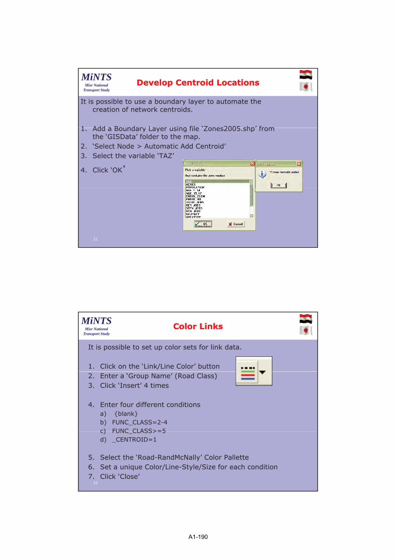
11
MiNTSMisr National
Transport Study
Develop Centroid LocationsDevelop Centroid Locations
It is possible to use a boundary layer to automate the creation of network centroids.
1 Add a Boundary Layer using file ‘Zones2005 shp’ from1. Add a Boundary Layer using file Zones2005.shp from the ‘GISData’ folder to the map.
2. ‘Select Node > Automatic Add Centroid’3. Select the variable ‘TAZ’
4. Click ‘OK’
21
MiNTSMisr National
Transport Study
Color LinksColor Links
It is possible to set up color sets for link data.
1. Click on the ‘Link/Line Color’ button2. Enter a ‘Group Name’ (Road Class)3. Click ‘Insert’ 4 times
4. Enter four different conditionsa) {blank}b) FUNC_CLASS=2-4c) FUNC CLASS>=5c) FUNC_CLASS>=5d) _CENTROID=1
5. Select the ‘Road-RandMcNally’ Color Pallette6. Set a unique Color/Line-Style/Size for each condition7. Click ‘Close’
22
A1-190

12
MiNTSMisr National
Transport Study
Link/Line Color DialogLink/Line Color Dialog
23
MiNTSMisr National
Transport Study
Develop Centroid ConnectorsDevelop Centroid Connectors
1. Now that the Centroids are created, we can automate the process of connecting them to the network.
1. Click the ‘View Center on Nodes’ button2. Enter Node Number ’14’ and Window Width ‘10000’3. Select ‘Node > Automatic Add Centroid Connections’4. Enter Maximum Number of Connectors (4)5 E t M i Di t f C ti (5000)5. Enter Maximum Distance for Connections (5000)6. Enter Directional Weighting Factor (4)7. Place a ‘Do NOT Connect to a Link’ condition
o FUNC_CLASS=1-2
24
A1-191

13
MiNTSMisr National
Transport Study
Automatic Centroid Connectors Automatic Centroid Connectors
25
MiNTSMisr National
Transport Study
Network ComputationsNetwork Computations
1. Select ‘Link > Compute’2. Name Set 1 (Connector Defaults)3. Right-Click in the open area, select ‘Append’g p , pp4. Enter the calculation (right-click to access variable list)
o SPEED=15
5. Append the following calculationso NUMLANES=2o ONEWAY_TWO=2o FUNC_CLASS=7
6 Apply a condition so only connectors are calculated6. Apply a condition so only connectors are calculatedo _CENTROID=1
7. Click Apply8. Click Close
26
A1-192
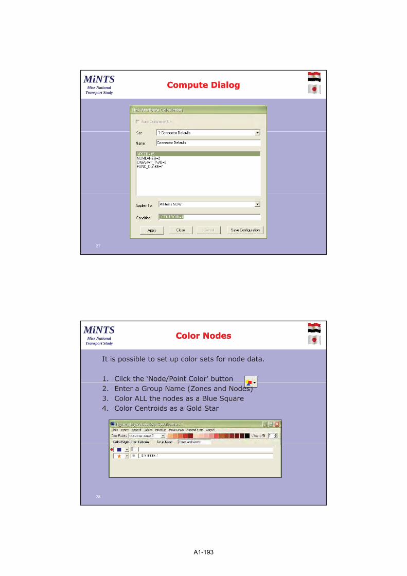
14
MiNTSMisr National
Transport Study
Compute DialogCompute Dialog
27
MiNTSMisr National
Transport Study
Color NodesColor Nodes
It is possible to set up color sets for node data.
1. Click the ‘Node/Point Color’ button2. Enter a Group Name (Zones and Nodes)3. Color ALL the nodes as a Blue Square4. Color Centroids as a Gold Star
28
A1-193
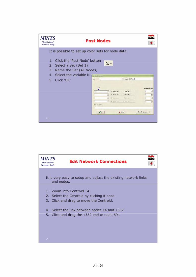
15
MiNTSMisr National
Transport Study
Post NodesPost Nodes
It is possible to set up color sets for node data.
1. Click the ‘Post Node’ button2. Select a Set (Set 1)3. Name the Set (All Nodes)4. Select the variable N
5. Click ‘OK’
29
MiNTSMisr National
Transport Study
Edit Network ConnectionsEdit Network Connections
It is very easy to setup and adjust the existing network links and nodes.
1. Zoom into Centroid 14.2. Select the Centroid by clicking it once.3. Click and drag to move the Centroid.
4. Select the link between nodes 14 and 1332l k d d h d d5. Click and drag the 1332 end to node 691
30
A1-194
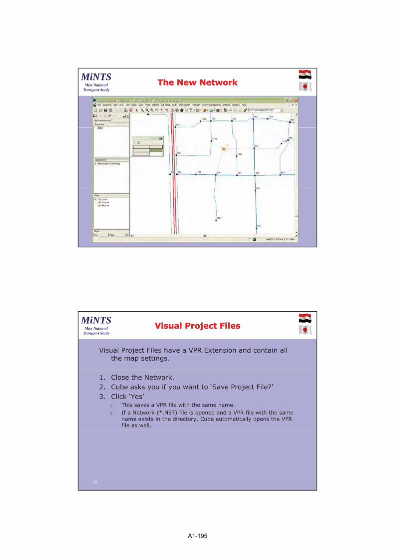
16
MiNTSMisr National
Transport Study
The New NetworkThe New Network
31
MiNTSMisr National
Transport Study
Visual Project FilesVisual Project Files
Visual Project Files have a VPR Extension and contain all the map settings.
1. Close the Network.2. Cube asks you if you want to ‘Save Project File?’ 3. Click ‘Yes’
o This saves a VPR file with the same name.o If a Network (*.NET) file is opened and a VPR file with the same
name exists in the directory, Cube automatically opens the VPR file as well.
32
A1-195
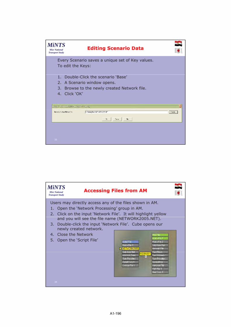
17
MiNTSMisr National
Transport Study
Editing Scenario DataEditing Scenario Data
Every Scenario saves a unique set of Key values. To edit the Keys:
1. Double-Click the scenario ‘Base’2. A Scenario window opens.3. Browse to the newly created Network file.4. Click ‘OK’
33
MiNTSMisr National
Transport Study
Accessing Files from AMAccessing Files from AM
Users may directly access any of the files shown in AM.1. Open the ‘Network Processing’ group in AM.2. Click on the input ‘Network File’. It will highlight yellow
d ll h f l ( )and you will see the file name (NETWORK2005.NET).3. Double-click the input ‘Network File’. Cube opens our
newly created network.4. Close the Network5. Open the ‘Script File’
34
A1-196

18
MiNTSMisr National
Transport Study
Script File StructureScript File Structure
35
MiNTSMisr National
Transport Study
Generated Script FilesGenerated Script Files
• When a script file are created and maintained by AM• AM automatically generate the basic structure• AM keeps track of all the input and output files
Th ill dd P P bl k• The user will add Parameters, Process blocks,Calculations
• The user should NEVER edit the file names and locations• All changes to the file names and locations should be
done in AM
36
A1-197

19
MiNTSMisr National
Transport Study
CommentsComments
Comment is any text following a ;(on the same line)o may be at start of lineo may be midway through a lineo may be midway through a commando Example
A=1 ;command followed by comment;comment line here
Block comment: enclosed by /* … */o Example
A=1 /* comments start hereA=1 / comments start here……
… comments end here */B=2
37
MiNTSMisr National
Transport Study
VoyagerVoyager Programs Programs ––a Revisiona Revision
• NETWORKo Building, Comparing and Manipulating Highway Networks
• HIGHWAYo Pathbuilding, Skimming, and Assignment of Highway
Networks
• PTo All Public Transit Functions
• GENERATIONo Trip Generation
• DISTRIBUTIONo Trip Distribution
• FRATARo Matrix Growth Factoring
• MATRIXo Demand Modeling and Matrix Manipulations
38
A1-198

20
MiNTSMisr National
Transport Study
HighwayHighway
• Primary function is to Build Paths between all IJ pairs• Once Paths are built, the user may:
o Skim network variableso Assign trips to network
• Input may includeo Highway networko Zonal matriceso Zonal data fileso Turn penalties
• Output may includeo Loaded networko Matriceso Junction Output Data
39
MiNTSMisr National
Transport Study
Highway PHASE=LINKREADHighway PHASE=LINKREAD
• Defines required values for each link.• Built-in Variables and Functions may be set here.y• Script:
o DISTANCE = (LI.SHAPE_LENG/5280) ;Link Distance in Miles
o T0 = (DISTANCE/LI.SPEED)*60 ;Free-Flow Time (Minutes)
40
A1-199

21
MiNTSMisr National
Transport Study
Highway PHASE=ILOOPHighway PHASE=ILOOP
• Builds paths from each origin zone to every destination• Script:p
o PATHLOAD ;Defines Processo PATH=TIME, ;Defines Impedance Variableo MW[1]=PATHTRACE(TIME) ;Skims Network Variable
41
MiNTSMisr National
Transport Study
Highway File DefinitionHighway File Definition
• The user needs to tell the output matrix what working matrixes will be saved.
• The user may name these matrices• Script (appended to MATO):
o MO=1, NAME=TIME
42
A1-200

22
MiNTSMisr National
Transport Study
Running ProgramsRunning Programs
As well as running entire models, AM provides the ability to run individual steps in the modeling process.
1. Navigate to the ‘Network Processing’ group.2. Double-Click the ‘Highway’ program box.
o The program runs.3. Examine the output Matrix4. Examine the output Print File
43
MiNTSMisr National
Transport Study
Highway FunctionsHighway Functions
Functions may be defined and used in the Highway program.Functions are usually placed in the LINKREAD PhaseScript:
o FUNCTION Cost = (Distance * 0.50) + (TIME * 0.20)
1. Define the Cost Function2. Use Cost as the Pathbuilding Impedance3. Skim Distance and Cost as well as time4. Save all 3 matrices
44
A1-201

23
MiNTSMisr National
Transport Study
Highway ScriptHighway Script
45
MiNTSMisr National
Transport Study
Cleaning Up the ApplicationCleaning Up the Application
1. Right-click the ‘Highway’ program2. Select ‘Hide unused files for program’
3. Right-click the ‘Highway’ program4. Select ‘Set Title’5. Label the program (Initial Free-Flow Highway Skims)
6. Right-Click on output ‘Matrix File 1’7 Select ‘Change File Description’7. Select Change File Description8. Label the file (Initial FF Skims)
46
A1-202

24
MiNTSMisr National
Transport Study
GenerationGeneration
• Primary function is to process zonal data and generate arrays of productions and attractions
• Calculations and balancing functions are user defined
• Input may include o Up to 10 zonal data files
• Output may includeUp to 10 production and attraction fileso Up to 10 production and attraction files
47
MiNTSMisr National
Transport Study
Generation PHASE=ILOOPGeneration PHASE=ILOOP
• In this step the stack of calculations are performed on each zone.
h ll d l l d• The user usually accessed a Zonal Data File andsupplies regression equations.
• Script:o P[1]=3.2*ZI.1.HOUSEHOLDSo P[2]=2.5*ZI.1.HOUSEHOLDSo P[3]=1.2*ZI.1.HOUSEHOLDSo A[1]=1.6*ZI.1.TOTAL_JOBSo A[2]=34 *ZI.1.TOTAL_JOBSo A[3]=19 *ZI.1.TOTAL_JOBS
48
A1-203
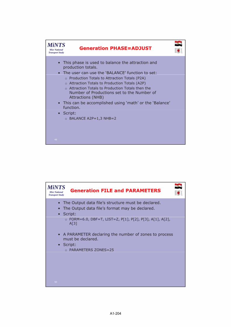
25
MiNTSMisr National
Transport Study
Generation PHASE=ADJUSTGeneration PHASE=ADJUST
• This phase is used to balance the attraction and production totals.
• The user can use the ‘BALANCE’ function to set: o Production Totals to Attraction Totals (P2A)o Attraction Totals to Production Totals (A2P)o Attraction Totals to Production Totals then the
Number of Productions set to the Number of Attractions (NHB)
• This can be accomplished using ‘math’ or the ‘Balance’ function.
• Script:o BALANCE A2P=1,3 NHB=2
49
MiNTSMisr National
Transport Study
Generation FILE and PARAMETERSGeneration FILE and PARAMETERS
• The Output data file’s structure must be declared.• The Output data file’s format may be declared.• Script:
o FORM=6.0, DBF=T, LIST=Z, P[1], P[2], P[3], A[1], A[2], A[3]
• A PARAMETER declaring the number of zones to process must be declared.
• Script:o PARAMETERS ZONES=25
50
A1-204

26
MiNTSMisr National
Transport Study
Preparing ‘Trip Distribution’Preparing ‘Trip Distribution’
• When we begin to look at the files for distribution, we see that the inputs for the matrix and the trip ends are coming from other programs.
• If we link these directly to the files, it will be static and will not change if we rename or change the output file.
• We need to instead link these to the other programs graphically in AM. This provides a ‘dynamic’ linkgraphically in AM. This provides a dynamic link
51
MiNTSMisr National
Transport Study
Public FilesPublic Files
In order to directly link files from the output side of one program processing step to the input side of another, they must be present on the same level.
For readability, it is best to have all files which are ‘external’ to the sub-group (overall input and outputs of the group) to be exposed to the parent application.
1. Browse to the Network Processing group 2. Right-click on the input Network File3. Select ‘Make File Public’4. Repeat for the output ‘Initial FF Skims’ file5. Repeat for the primary input and output files in:
a) Trip Generationb) Trip Distribution
52
A1-205

27
MiNTSMisr National
Transport Study
Exposed FilesExposed Files
53
MiNTSMisr National
Transport Study
Linking FilesLinking Files
To create a direct (dynamic) link between program files, simply highlight the output file you want to connect ‘from’ and then click and drag a link to the file you
ant to connect ‘to’want to connect ‘to’
1. Click on the output ‘Initial FF Skims’ file2. Click and drag a link onto the input ‘Impedance Matrix’
file
54
A1-206

28
MiNTSMisr National
Transport Study
DistributionDistribution
• Uses the number of trip ends in each zone as the starting point. These ‘margin’ totals are distributed to the rows and column of a generated matrix.
• The distribution is weighted by the ‘Impedance’• The impedance is calibrated with a Friction Factor Curve.• Most common process is the "gravity" model, but there is
no automatic, or default, trip distribution process.• Input may include:
o Up to 20 matrix fileso Up to 20 matrix files o 1 text data file of data (friction factors)o Up to 10 production and attraction files
• Output may include:o Up to 32 trip matrix files
55
MiNTSMisr National
Transport Study
Distribution PARAMETERSDistribution PARAMETERS
• To control the number of iterations, it is possible to set the convergence thresholds as well as the maximum number of iterations.
• Script:PARAMETERS MAXITERS=99,MAXRMSE=5
56
A1-207

29
MiNTSMisr National
Transport Study
Distribution SETPADistribution SETPA
• The initial values to use for the row and column totals need to be set.
• These will be equal to the number of Productions and Attractions calculated in trip generation.
• Script: SETPA P[1]=ZI.1.P1, A[1]=ZI.1.A1,
P[2]=ZI.1.P2, A[2]=ZI.1.A2,P[3]=ZI.1.P3, A[3]=ZI.1.A3
57
MiNTSMisr National
Transport Study
LOOKUP FunctionsLOOKUP Functions
Traditionally the Friction Factors are described with a Lookup function.Script:LOOKUP NAME=FF, ;Declare a function nameLOOKUP NAME=FF, ;Declare a function nameLOOKUP[1]=1, RESULT=2, ;Curve 1 definitionLOOKUP[2]=1, RESULT=3, ;Curve 2 definitionLOOKUP[3]=1, RESULT=4, ;Curve 3 definitionINTERPOLATE=Y, ;Interpolate to define missing valuesR= ‘0.01 1200 1000 800’,
‘1 1000 900 700’,‘5 500 400 300’,‘ 200 0 ’‘7 200 150 75’,‘10 100 75 25’,‘25 50 50 10’,‘50 5 5 5’
58
A1-208

30
MiNTSMisr National
Transport Study
Distribution GRAVITY FunctionDistribution GRAVITY Function
GRAVITY Function: Performs distribution based on traditional gravity modelo PURPOSE can be applied to different ‘purpose’ matrices
LOS defines the cost matriceso LOS defines the cost matriceso FFACTORS defines the impedance curveo KFACTORS allows additional weighting
Script:MW[20] = MI.1.COSTGRAVITY PURPOSE=1, LOS=MW[20], FFACTORS=FFGRAVITY PURPOSE=2, LOS=MW[20], FFACTORS=FFGRAVITY PURPOSE=3, LOS=MW[20], FFACTORS=FF
59
MiNTSMisr National
Transport Study
Distribution AdditionalDistribution Additional
• Create a Total Trips matrix• Name the matrices
o HBWo HBOo NHBo Total
60
A1-209

31
MiNTSMisr National
Transport Study
MatrixMatrix
• Matrix is primarily a calculator. It simply processes matrices, zonal data, or text records according to user specified expressions.
• Inputs may include:Inputs may include:o Matriceso Zonal data fileso Record Data files
• Outputs may include:o Matriceso Print Data fileso Record files
• Various file formats for both input and output are supported
• User is responsible for specifying what is to be accomplished
61
MiNTSMisr National
Transport Study
MatrixMatrix –– Common UsesCommon Uses
Commonly used to:• Calculate new matrix values• Convert and merge matrices between various
fformats
• Report values from matrices and zonal data by:o Selected rowso Marginal summaries (trip ends, etc.)o Frequency distributions
• Transpose matrices• Generate matrices• Renumber, aggregate, and disaggregate matrices• Process Record data
62
A1-210
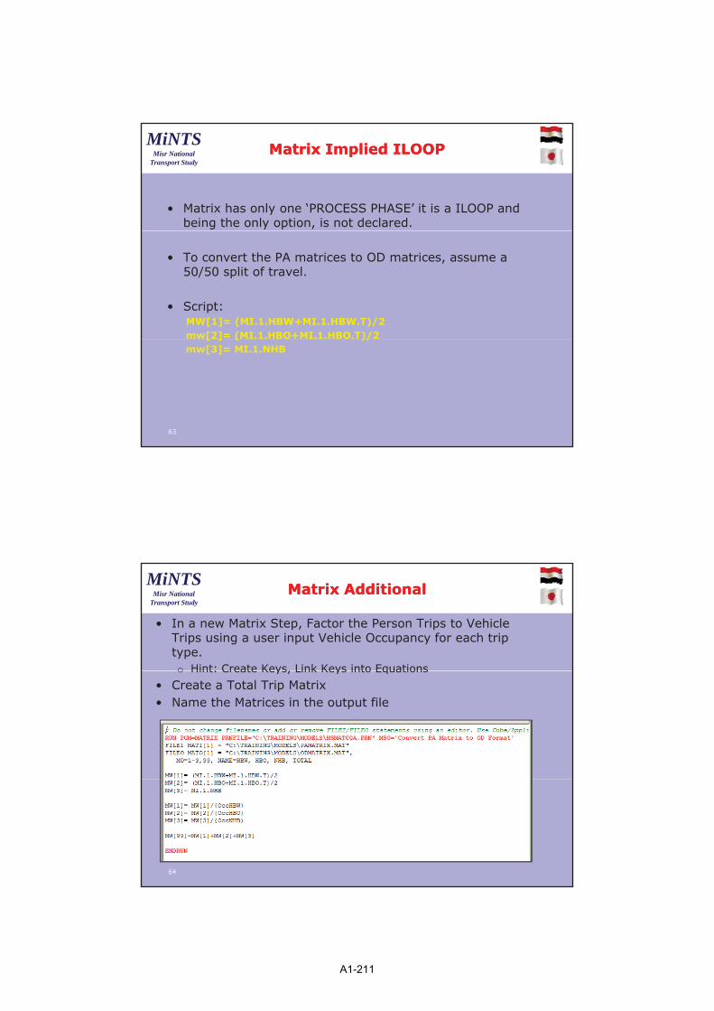
32
MiNTSMisr National
Transport Study
Matrix Implied ILOOPMatrix Implied ILOOP
• Matrix has only one ‘PROCESS PHASE’ it is a ILOOP and being the only option, is not declared.
• To convert the PA matrices to OD matrices, assume a 50/50 split of travel.
• Script:MW[1]= (MI.1.HBW+MI.1.HBW.T)/2mw[2]= (MI.1.HBO+MI.1.HBO.T)/2[ ] ( )/mw[3]= MI.1.NHB
63
MiNTSMisr National
Transport Study
Matrix AdditionalMatrix Additional
• In a new Matrix Step, Factor the Person Trips to Vehicle Trips using a user input Vehicle Occupancy for each trip type.o Hint: Create Keys, Link Keys into Equationso Hint: Create Keys, Link Keys into Equations
• Create a Total Trip Matrix• Name the Matrices in the output file
64
A1-211
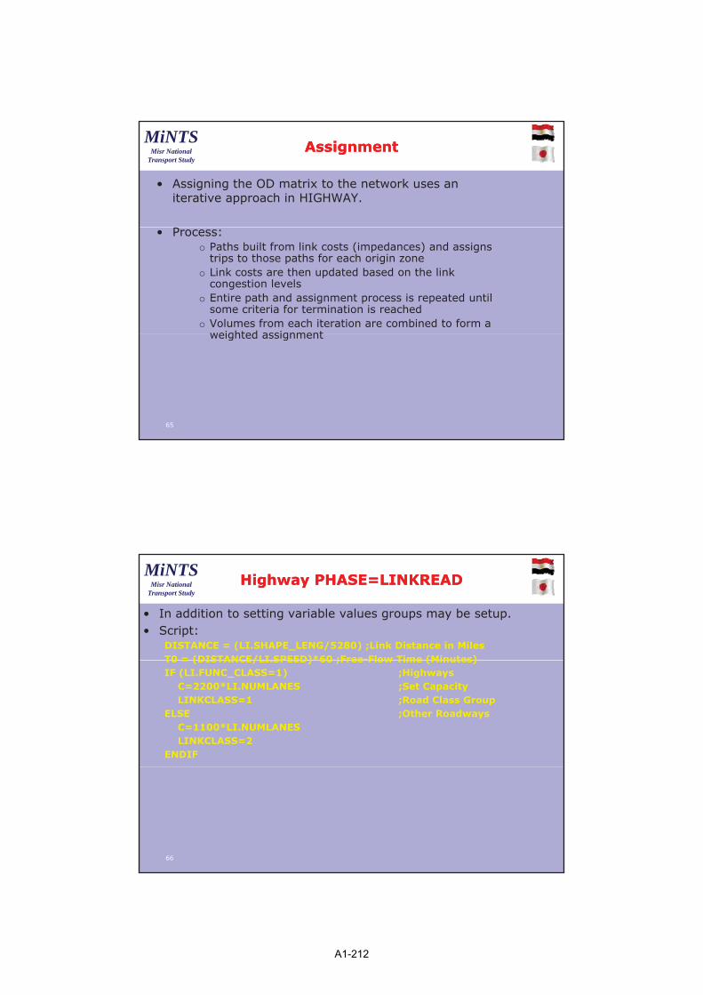
33
MiNTSMisr National
Transport Study
AssignmentAssignment
• Assigning the OD matrix to the network uses an iterative approach in HIGHWAY.
• Process:o Paths built from link costs (impedances) and assigns
trips to those paths for each origin zoneo Link costs are then updated based on the link
congestion levelso Entire path and assignment process is repeated until
some criteria for termination is reachedo Volumes from each iteration are combined to form a
weighted assignmentweighted assignment
65
MiNTSMisr National
Transport Study
Highway PHASE=LINKREADHighway PHASE=LINKREAD
• In addition to setting variable values groups may be setup.• Script:
DISTANCE = (LI.SHAPE_LENG/5280) ;Link Distance in MilesT0 = (DISTANCE/LI SPEED)*60 ;Free-Flow Time (Minutes)T0 = (DISTANCE/LI.SPEED) 60 ;Free Flow Time (Minutes)IF (LI.FUNC_CLASS=1) ;Highways
C=2200*LI.NUMLANES ;Set CapacityLINKCLASS=1 ;Road Class Group
ELSE ;Other RoadwaysC=1100*LI.NUMLANESLINKCLASS=2
ENDIF
66
A1-212

34
MiNTSMisr National
Transport Study
Highway PHASE=LINKREADHighway PHASE=LINKREAD
• In addition to setting variable values and groups, functions may also be setup.
• Functions are defined for individual Link Classes (Undefined Classes use Class 1)
• One FUNCTION statement can be used to define a number of functions by grouping them with {…}
• Script:FUNCTION {
tc[1]=t0*(1.0+0.15*((v/c)^8))tc[2]=t0*(1.0+0.15*((v/c)^4))
t[1] TIME*0 2 DISTANCE*0 8cost[1]=TIME*0.2+DISTANCE*0.8cost[2]=TIME*0.2+DISTANCE*0.5}
67
MiNTSMisr National
Transport Study
Highway PHASE=ILOOPHighway PHASE=ILOOP
• Builds paths from each origin zone to every destination
• Keywords Can be added to assign Volume Sets. If present, this will force it into a iterative assignment process.
• Script:
PATHLOAD ;Defines ProcessPATH=TIME ;Defines Impedance VariablePATH=TIME, ;Defines Impedance VariableVOL[1]=MI.1.PCTOTAL
68
A1-213

35
MiNTSMisr National
Transport Study
Add Path FileAdd Path File
• Path Files are a complete record…
• Script (within path-load)
PATHO=1, ;Path File Number to save toNAME=‘PT Loads', ;Path set nameALLJ=T, ;save all paths even 0 trip interchangesINCLUDECOSTS=T ;save costs as well as paths
69
MiNTSMisr National
Transport Study
Live DemonstrationLive Demonstration
• Viewing Path File Data
• Adding Map Layers
• Drawing Layers
• Add Truck Volumes
• Running the Application
• Appliers Mode
• Creating Scenarios
• Scenario Specific Files70
A1-214

36
MiNTSMisr National
Transport Study
Public Transport (PT)Public Transport (PT)
• Key Featureso ‘True’ Multi-Routing Between Zoneso Demand Stratification by User Classo Comprehensive Fares Modelingp g
• Handles all aspects of assigning trips to a public transport network
o Network Buildingo Route Enumerationo Route Evaluationo Skimmingo Loading (Assignment)o Analysis (Reporting)o Analysis (Reporting)
• The PT Models:o Determine the probability of use for alternative routeso Trips are then loaded on the routes based upon these
probabilities
71
MiNTSMisr National
Transport Study
PT Network DevelopmentPT Network Development
• A Network, produced by NETWORK, PUBLIC TRANSPORT (PT), or the User containing:
o Characteristics of zoneso Links and Nodeso Walk and Transit travel timeso Distance etc
• System information o used to describe the characteristics such as modes, operators and
waiting curves• Service or Line data
o Describes the Routes and Stops• Non Transit Legs Records possible ways to:• Non-Transit Legs - Records possible ways to:
o Access the Public Transport Systemo Egress from the Public Transport Systemo Transfer between services during the course of a journey.
(Non-transit legs may be determined externally and/or generated by Public Transport under user control.)
72
A1-215

37
MiNTSMisr National
Transport Study
PT Route Enumeration & PT Route Enumeration & EvaluationEvaluation
• Determines 'reasonable' or 'attractive' multiple discrete routes between zones.
k (b l )• May take into account (by user class):o Number of transferso Spreado The margin of cost over the minimum cost route;o Non-transit and In-Vehicle Costso Boarding and Transfer Penalties by mode;o Waiting Timeo Derived from the combined frequency of services betweeno Derived from the combined frequency of services between
stop nodeso Fares (considered only for Evaluation)
73
MiNTSMisr National
Transport Study
PT Skimming PT Skimming
• Skimming extracts:o Composite costso Value of Choiceo Perceived and Actual journey costsj y
� Non-Transit Costs� In-vehicle and Wait times� Boarding and transfer penalties (Fares)
o Best journey cost
• Journey costs may be extracted Network Wide or Stratified by Mod• Used for:
o Model validationD d d lio Demand modeling
o Scheme evaluationo Loading demand on the networks o Producing operational statistics (passenger miles, hours, and
revenue)
74
A1-216

38
MiNTSMisr National
Transport Study
PT Assignment (Loading)PT Assignment (Loading)
• Loads demand, in the form of trips between zone pairs
• Uses a series of models during a journey:o The Walk Choice Model
� Allocates trips between attractive choices at access, egress and transfer points.
o The Service Frequency & Cost Model� Allocates the transit share at a stop between the
attractive services available at that stopo The Alternative Alighting Model
� Apportions the share of a service to the attractive alternative alighting points of that service g g p
75
MiNTSMisr National
Transport Study
Creating a PT NetworkCreating a PT Network
1. Click on the Layer control icon .2. Check on the Transit Layer 3. The Open TRNLAYER Layer Parameters dialog
opens4. Click Browse5. Save C:\Training\example.lin 6. Click ‘Open’7. Click ‘Yes’ to create this new file.8. Select ‘Voyager PT Line Format’y g9. Select ‘Voyager PT Line Format’10.Click ‘All Done’
76
A1-217

39
MiNTSMisr National
Transport Study
PT Line ManagerPT Line Manager
The public transit line manager shows the transit files that are available for editing as well as the transit lines that are currently in the file.
1. Set the TRN Layer to the ‘Active’ or top most layer
2. Click Line Manager.
3. Click New in Line Options.p
4. Type in the Name (Red Flash)
5. Click OK. • The dialog box closes and we now have created a transit line. 77
MiNTSMisr National
Transport Study
PT Line Manager DialogPT Line Manager Dialog
78
A1-218

40
MiNTSMisr National
Transport Study
Preparing to Edit the PT LinePreparing to Edit the PT Line
1. With Red Flash highlighted, click on Edit. • The transit line coding dialog opens.
2. Click on the ‘zoom to node’ icon3. Enter node 791. 4. Set Window Width to 250005. Click OK. 6. Select ‘Post > One-Way Arrow’7. Post all node numbers
79
MiNTSMisr National
Transport Study
Editing a PT LineEditing a PT Line
1. Click on the Route Edit button on the dialog • If you move the cursor over the map, you should now have a
cross-hair.
2. Click on Node 797 3. Click on Node 791 to create the next Transit Stop. The
Route is extended the route to that node.4. Alt+Click on Node 784 to simply extend the route to this
node. No Transit Stop is created.5. Continue the Route into Downtown5. Continue the Route into Downtown6. Press ESC to exit Route Creation Mode7. Click the ‘Green Check-Mark’ to save the updates
80
A1-219

41
MiNTSMisr National
Transport Study
Editing PT Line ParametersEditing PT Line Parameters
1. Fully enlarge the PT Rote Edit Dialog Window• Each Node in the Route is present• Non-Stop Nodes are designated by a ‘-’ sign. No boarding or
alighting will be allowed.
2. In the ‘Mode’ variable, enter mode number (1)3. Click on the ‘Insert Row’ Button
• The dialog lists all possible line parameters that may be used
4. Double-Click ‘Headway[1]’5. Double-Click ‘Color’6. Click ‘Cancel’7 E C l C d (3)7. Enter a Color Code (3)8. Enter a Headway Time (10)9. Save the Changes
81
MiNTSMisr National
Transport Study
Viewing PT LinesViewing PT Lines
1. Click the Transit Line Manager Button
2 Click ‘Save All’ to save edits2. Click Save All to save edits.
3. Click ‘Exit’
4. Select ‘Transit > Show Stop/Non-Stop Nodes’
5. Check the two check boxes and accept the default colors pand sizes. Click OK.
6. The transit line now shows where it runs, where it stops and where it does not stop.
82
A1-220

42
MiNTSMisr National
Transport Study
More PT Line EditingMore PT Line Editing
• Code another bus line named ‘Blue Dragon’
• mode=1, headway[1]=15, color=1
• Modify an existing transit line.
83
MiNTSMisr National
Transport Study
Coding PT Mode DataCoding PT Mode Data
1. In Transit Line Manager, Click Open
2. Create a new transit file (TransitSystemData.pts)2. Create a new transit file (TransitSystemData.pts)
3. Click on ‘System Data’
4. Set access mode definitions: • Mode=1, Name="NatRail", Longname="NationalRailways"• Mode=2, Name=“RegRail", Longname="RegionalRailways"• Mode=3, Name="ExpBus", Longname="ExpressBuses"• Mode=4, Name="LocBus", Longname="LocalBuses"• Mode=33, Name="Walk", Longname="walk access connectors"• Mode=34, Name="Xwlk", Longname="walk transfer connectors”
84
A1-221

43
MiNTSMisr National
Transport Study
Code PT Waiting DataCode PT Waiting Data
1. In the Transit Line Manager, Click ‘Curve/Profile’2. Click ‘Add Curve’3. Enter the Name (Short, Short Wait)4. Enter the Curve Definition (1-0.5,15-5.0,100-10.0)5. Click the Green Check to Save6. Add a second Curve
• WAITCRVDEF=2, Name="Long-wait", Curve=1-0.5,15-7.5,100-20.0
7 Close the Curve Definition Window7. Close the Curve Definition Window8. Click ‘Save All’9. Click ‘Exit’
85
MiNTSMisr National
Transport Study
Viewing PT Coding in Cube TownViewing PT Coding in Cube Town
1. Network Building
2. Skimming
3. Mode Split
4. Assignment
86
A1-222
Related Documents