Stability, Protection and Control of Systems with High Penetration of Converter Interfaced Generation Final Project Report S-56 Power Systems Engineering Research Center Empowering Minds to Engineer the Future Electric Energy System

Welcome message from author
This document is posted to help you gain knowledge. Please leave a comment to let me know what you think about it! Share it to your friends and learn new things together.
Transcript

Stability, Protection and Control of
Systems with High Penetration of
Converter Interfaced Generation
Final Project Report
S-56
Power Systems Engineering Research Center
Empowering Minds to Engineer the Future Electric Energy System

Stability, Protection and Control of Systems with High
Penetration of Converter Interfaced Generation
Final Project Report
S-56
Project Team
Sakis A. P. Meliopoulos, Project Leader
Maryam Saeedifard
Georgia Institute of Technology
Vijay Vittal
Rajapandian Ayyanar
Arizona State University
Graduate Students
Yu Liu
Sanghun Choi
Evangelos Polymeneas
Georgia Institute of Technology
Deepak Ramasubramanian
Ziwei Yu
Arizona State University
PSERC Publication 16-03
March 2016

i
Acknowledgements
This is the final report for the Power Systems Engineering Research Center (PSERC) research
project S-56 titled “Stability, Protection and Control of Systems with High Penetration
of Converter-Interfaced Generation”. We express our appreciation to PSERC and the industry
advisors. We also express our appreciation to RTE for their support of the project and their close
collaboration in this project. We also express our appreciation for the support provided by the
National Science Foundation’s Industry / University Cooperative Research Center program.
The authors wish to recognize Thibault Prevost of RTE for his contributions to the project and
his guidance in discussing and formulating the issues related to systems with high penetration of
renewables.
The authors wish to recognize the postdoctoral researchers and graduate students at the Georgia
Institute of Technology who contributed to the research and creation of project reports:
Yu Liu
Sanghun Choi
Evangelos Polymeneas

ii
Executive Summary
The goal of this project is to evaluate the stability, protection and control of converter-interfaced
generation both at the converter level and in the bulk power system. With the increased penetration
of renewable energy and decommissioning of aging thermal power plants, there is a renewed focus
on converter-interfaced generation. As more of these sources appear in the transmission system,
the control of converters and their representation in software have to be more accurate in order to
make a reliable study of the system behavior.
This research proposes a new converter model for use in positive sequence transient stability
software. The questions addressed include- Does this converter model accurately represent the
electromagnetic transient operation of a power electronics converter? Does the model perform
robustly in commercial positive sequence time domain software? With large system simulations,
is there a significant increase in computation time with the use of this converter model? Can a
large system handle an increased presence of converter-interfaced generation? Will the converter
models be able to provide frequency response in the event of a contingency?
Part I: Stability, Protection and Control of Systems with High Penetration of
Converter Interfaced Generation
Increasing penetration of generating units that are interfaced to power grid with power electronic
devices create new challenges in the protection, control and operation of the power grid. These
generating units are allowed to operate at variable or non-synchronous frequencies (e.g. wind
turbines), or to operate without any rotating parts (e.g. photovoltaic cells) and they are
synchronized to the power grid via power electronics. We refer to these units as Converter-
Interfaced Generation (CIG). The power grid operates at a fixed frequency or a regulated frequency.
The power system can easily cope with a small amount of CIGs. However, in some areas of the
world, the percentage of CIGs versus synchronous machines has risen to high values and it is
possible to reach 100%. High penetration levels bring serious challenges to the present protection,
control and operation paradigm.
The conventional power system powered by synchronous generators has the following
characteristics. (a) synchronous generators are driven by mechanical torque, so the control of the
speed governor can maintain load/generation balance by controlling the frequency of the
synchronous generator; (b) synchronous generators have high moment of inertia, so the oscillations
of frequency and phase angle are small and slow, and transient stability of the power system can
be ensured. These characteristics are absent in CIGs. In conventional systems, frequency constancy
means generation/load balance. In systems with 100% CIGs this concept does not exist.
Compared to the conventional power system, a power system with high penetration of CIGs will
confront the following challenges. (a) There exists no mechanical torque input to the DC link of a
grid side converter, thus the control of the converter output frequency is irrelevant to
load/generation balancing [2-3]. Traditional control schemes, such as area control error (ACE)
become meaningless in systems with 100% CIGs. (b) CIGs do not have inertia [4-5], thus the
frequency and phase angle may oscillate quickly after disturbances and in this case the operational
constraints of the inverters may be exceeded to the point of damaging the inverters or causing the

iii
shutdown of the inverters. Inverters can be protected with Low Voltage Ride Through (LVRT)
function. However, in a system with high penetration of CIGs, the LVRT function practically
removes a large percentage of generation for a short time (typically 0.15 to 0.2 seconds). It is not
clear whether the system will gracefully recover from such an event.
One existing approach to deal with these issues is to control the converter interface such that the
CIG systems behave similarly as synchronous machines with frequency responses and inertia [6-
7]. However, this approach is not as good as expected because it is practically impossible to
achieve high synchronizing torques due to current limitations of the inverter power electronics.
For traditional power systems, synchronous machines can provide transient currents in the order
of 500% to 1000% of load currents. On the contrary, the converters have to limit the transient
currents to no more than approximately 170% of load currents for one or two cycles and further
decrease this value as time evolves [8]. Consequently, the CIGs’ imitation of synchronous
machines is not quite effective.
The first important problem is the recognition that fault currents in a system with high penetration
of CIGs will be much lower than conventional systems and many times may be comparable to load
currents. The issue has been addressed in this project. The findings are summarized in reference
[M1] listed in section 7. This reference shows the transformation of the fault currents as the
penetration of CIGs goes from 0% to 100%. The reduced fault currents create protection gaps for
these systems, in other words the system cannot depend on traditional protection schemes to
reliably protect against all faults and abnormal conditions. We propose a new approach to
protection based on dynamic state estimation.
The second important problem is the stabilization of CIGs with the power grid during disturbances.
To control the CIGs such that the CIG smoothly follows the oscillations of the system and avoids
excessive transients, a Dynamic State Estimation (DSE) enabled supplementary predictive inverter
control (P-Q mode) scheme has been proposed, implemented and tested. The method is based on
only local side information and therefore no telemetering is required and associated latencies. The
method consists of the following two steps: Step 1: The power grid frequency as well as rate of
frequency change is estimated using only local measurements and the model of the transmission
circuit connecting a CIG to the power grid. Step 2: The power grid frequency as well as rate of
frequency change are injected into the inverter controller to initiate supplementary control of the
firing sequence. The supplementary control amounts to predictive control to synchronize the
inverter with the motion of the power grid. Numerical experiments indicate that the supplementary
control synchronizes CIGs with the power grid in a predictive manner, transients between CIGs
and the power grid are minimized. One can deduct that the supplementary controls will minimize
instances of LVRT logic activation.
The application of the proposed method requires an infrastructure that enables dynamic state
estimation at each CIG. The technology exists today to provide the required measurements and at
the required speeds to perform dynamic state estimation. In essence the method provides full state
feedback for the control of the CIGs. While in this project we experimented with one type of
supplementary control, the ability to provide full state feedback via the dynamic state estimation
opens up the ability to use more sophisticated control methodologies. Future work should focus
on utilizing the dynamic state estimation to provide full state feedback and investigate additional

iv
control methods. The methods should be integrated with resource management, for example
managing the available wind energy (in case of a WTS) or the PV energy, especially in cases that
there is some amount of local storage. The dynamic state estimation based protection, should be
integrated in such a system.
Part II: Development of Positive Sequence Converter Models and
Demonstration of Approach on the WECC System
A voltage source representation of the converter-interfaced generation is proposed. The operation
of a voltage source converter serves as a basis for the development of this model wherein the
switching of the semiconductor devices controls the voltage developed on the ac side of the
converter. However, the reference current determines the value of this voltage. With the voltage
source representation, the filter inductance value plays an important role in providing a grounding
connection at the point of coupling. A point on wave simulation served as a basis for the calibration
of the proposed positive sequence model. Simulation of a simple two-machine test system and the
three-machine nine-bus WSCC equivalent system validated the performance of the model with
comparison against the existing boundary current injection models that are presently in use. In the
existing models, the absence of the filter inductance causes significant voltage drops at the terminal
bus upon the occurrence of a contingency and in a large system, it can lead to divergence of the
network solution. It was found that the voltage source representation was a more realistic
representation of the converter and was proposed to be used in all large-scale system studies.
The 2012 WECC 18205 bus system was used as a test system for large-scale system studies.
Initially, converters replaced only the machines in the Arizona and Southern California area and
the response to various system contingencies was analyzed. Carrying this forward, converters
replaced all machines in the system resulting in a 100% converter-interfaced generation set. The
performance of this system was found to be largely satisfactory. With the absence of rotating
machines, a numerical differentiation of the bus voltage angle gave an approximate representation
of the frequency. For the trip of two Palo Verde units, the frequency nadir was well above the
under frequency trip setting of the WECC system and the recovery of the frequency was within 2-
3 seconds enabled by the fast action of the converters. For other contingencies, the voltage
response of the individual units reflected the fast control action with the achievement of steady
state again within 2-3 seconds following the disturbance. Incorporation of overcurrent and
overvoltage protection mechanisms ensured adherence to the converter device limits.
An induction motor drive model was also developed and tested in an independent C code written
to perform a time domain positive sequence simulation. The performance of the nine bus system
with and without induction motor drives was analyzed.
Project Publications:
1. Ramasubramanian, D.; Z. Yu, R. Ayyanar and Vijay Vittal. “Converter Control Models for
Positive Sequence Time Domain Analysis of Converter Interfaced Generation,” submitted to
the IEEE Transactions – under review.

v
2. Ramasubramanian, D.; and Vijay Vittal. “Transient Stability Analysis of an all Converter
Interfaced Generation WECC System,” Submitted to the Power Systems Computation
Conference 2016 – abstract accepted.
3. Liu, Yu; Sakis A.P. Sakis Meliopoulos, Rui Fan, and Liangyi Sun. "Dynamic State
Estimation Based Protection of Microgrid Circuits," Proceedings of the IEEE-PES 2015
General Meeting, Denver, CO, July 26-30, 2015.
4. Liu, Yu; Sanghun Choi, A.P. Sakis Meliopoulos, Rui Fan, Liangyi Sun, and Zhenyu Tan.
“Dynamic State Estimation Enabled Predictive Inverter Control,” Accepted, Proceedings of
the IEEE-PES 2016 General Meeting, Boston, MA, July 17-21, 2016.
Student Theses:
1. Ramasubramanian, D. “Impact of Converter Interfaced Generation on Grid Performance,”
Ph.D. Thesis, Arizona State University, Tempe, AZ, 2016.
2. Weldy, Christopher. “Stability of a 24-Bus Power System with Converter Interfaced
Generation,” Master Thesis, Georgia Institute of Technology, Atlanta, GA, 2015.

Part I
Stability, Protection and Control of Systems with
High Penetration of Converter Interfaced Generation
Sakis A. P. Meliopoulos, Project Leader
Maryam Saeedifard
Georgia Institute of Technology
Graduate Students
Yu Liu
Sanghun Choi
Evangelos Polymeneas
Georgia Institute of Technology

ii
For more information about Part I, contact:
Sakis A.P. Meliopoulos
Georgia Institute of Technology
School of Electrical and Computer Engineering
777 Atlantic Dr. NW
Atlanta, Georgia 30332-0250
Phone: 404-894-2926
E-mail: [email protected]
Power Systems Engineering Research Center
The Power Systems Engineering Research Center (PSERC) is a multi-university Center
conducting research on challenges facing the electric power industry and educating the next
generation of power engineers. More information about PSERC can be found at the Center’s
website: http://www.pserc.org.
For additional information, contact:
Power Systems Engineering Research Center
Arizona State University
551 E. Tyler Mall
Engineering Research Center #527
Tempe, Arizona 85287-5706
Phone: 480-965-1643
Fax: 480-965-0745
Notice Concerning Copyright Material
PSERC members are given permission to copy without fee all or part of this publication for internal
use if appropriate attribution is given to this document as the source material. This report is
available for downloading from the PSERC website.
2016 Georgia Institute of Technology. All rights reserved.

iii
Table of Contents
1. Introduction ............................................................................................................................ 1
1.1 Background ................................................................................................................. 1
1.2 Motivation and Objectives .......................................................................................... 2
1.3 Organization of the Report .......................................................................................... 4
2. Literature Review .................................................................................................................. 5
3. Proposed Technologies – Dynamic State Estimator ............................................................. 6
3.1 Dynamic State Estimator (DSE) with Local Information Only .................................. 8
3.2 Digital Signal Processor (DSP) ................................................................................. 11
3.3 Physically-Based Inverter Modeling ......................................................................... 11
4. Proposed Technologies – Supplementary Predictive Inverter Control ............................... 14
4.1 DSE Enabled Supplementary Predictive Inverter Control ........................................ 14
4.2 Frequency-Modulation Control ................................................................................. 15
4.3 Modulation-Index and Phase-Angle Modulation Control ......................................... 15
4.4 Switching-Sequence Modulation Control ................................................................. 17
5. Simulation Results ............................................................................................................... 25
5.1 Performance Evaluation of the Dynamic State Estimator (DSE) ............................. 25
5.2 Performance Evaluation of the Supplementary Predictive Inverter Control Enabled by
Dynamic State Estimator (DSE) ............................................................................... 33
5.2.1 Case 1: WTS Performance Without Proposed Control Strategy .................... 35
5.2.2 Case 2: WTS Performance With Proposed Control Strategy ......................... 36
6. Conclusions and Future Work ............................................................................................. 37
7. Publications as Direct Result of this Project ....................................................................... 38
8. References ........................................................................................................................... 39
9. Appendix A: The Quadratic Integration Method ............................................................... 43
10. Appendix B: Model Description of Three-Phase Transmission Line ................................ 48
B-1: QDM of single-section transmission line model ....................................................... 48
B-2: QDM of multi-section transmission line model ........................................................ 49
11. Appendix C: Model Description of Three-Phase Two-Level PWM Inverter .................... 51
C-1: verall Model Description ........................................................................................... 51
C-2: Single Valve Model ................................................................................................... 55
C-3: DC-side capacitor model ............................................................................................. 62
12. Appendix D: Model Description of the Digital Signal Processor (DSP) ........................... 64
D-1: Frequency and the Rate of Frequency Change.......................................................... 64
D-2: Positive Sequence Voltage Phasor ............................................................................ 69

iv
D-3: Positive-Sequence Current Phasor ............................................................................ 70
D-4: Fundamental Frequency Real and Reactive Power ................................................... 71
D-5: Next Zero-Crossing Time.......................................................................................... 71
D-6: Average DC-Input Voltage ....................................................................................... 73
13. Appendix E: Master Thesis by Christopher Weldy............................................................ 74
v
List of Figures
Figure 3-1: Overall Approach for Protection, Control and Operation of a CIG ............................ 6
Figure 3-2: Dynamic State Estimator with Local Measurement Only .......................................... 9
Figure 3-3: Dynamic State Estimation Operating on Two Consecutive Sets of Measurements ... 9
Figure 3-4: Multi-Section Transmission Line Model .................................................................. 10
Figure 3-5: Single-Section Three-Phase Transmission Line Model ............................................ 10
Figure 3-6: Block Diagram of the Digital Signal Processor ........................................................ 11
Figure 3-7: Three-Phase Two-Level PWM Inverter Model ........................................................ 12
Figure 3-8: Single Valve Model .................................................................................................. 13
Figure 4-1: Block Diagram of the Supplementary Predictive Inverter Control (P-Q Mode) ...... 14
Figure 4-2: Base Switching Sequence of the Phase A ................................................................. 19
Figure 4-3: Base Switching Sequence of the Phase B ................................................................. 19
Figure 4-4: Base Switching Sequence of the Phase C ................................................................. 20
Figure 4-5: Modulated Switching-Signal Sequence of the Phase A (SWA_UP) ........................ 22
Figure 4-6: Modulated Switching-Signal Sequence of the Phase B (SWB_UP)......................... 23
Figure 4-7: Modulated Switching-Signal Sequence of the Phase C (SWC_UP)......................... 24
Figure 5-1: Simulation System for Frequency Estimation .......................................................... 25
Figure 5-2: Simulation Results, 1.5-Mile Line, Local Side ......................................................... 26
Figure 5-3: Simulation Results, 1.5-Mile Line, Remote Side...................................................... 27
Figure 5-4: Simulation Results, 2.5-Mile Line, Local Side ......................................................... 28
Figure 5-5: Simulation Results, 2.5-Mile-Line, Remote Side ..................................................... 29
Figure 5-6: Simulation Results, 4-Mile Line, Local Side ............................................................ 30
Figure 5-7: Simulation Results, 4-Mile Line, Remote Side......................................................... 31
Figure 5-8: Test Bed for the Supplementary Predictive Inverter Control ................................... 33
Figure 5-9: Simulation Result when the Proposed Control Is Disabled ...................................... 35
Figure 5-10: Simulation Results when the Proposed Control is Enabled .................................... 36
Figure A-1: Illustration of the Quadratic Integration Method ..................................................... 43
Figure B-1: The Single-Section Three-Phase Transmission Line Model .................................... 48
Figure B-2: Multi-section transmission line model ..................................................................... 49
Figure C-1: Three-Phase Two-Level PWM Inverter Model........................................................ 51
Figure C-2: The Single Valve Model........................................................................................... 52

vi
Figure C-3: Three-Phase Two-Level PWM Inverter Model with Assigned Node Numbers ...... 53
Figure C-4: Procedure of the Generation of the SCAQCF of the Inverter Model ....................... 54
Figure C-5: DC-Side Capacitor Model ........................................................................................ 62
Figure D-1: Block Diagram of the Digital Signal Processor ....................................................... 64
Figure D-2: Cosine Function with respect to the Phase Angle .................................................... 72

vii
List of Tables
Table 5-1: Results of Side 1 ......................................................................................................... 32
Table 5-2: Results of Side 2 ......................................................................................................... 32
Table 5-3: List of the Components of the Test Bed ..................................................................... 34
Table C-1: Assigned Node Numbers of the Three-Phase Two-Level PWM Inverter ................. 55

1
1. Introduction
1.1 Background
Power systems around the world are seeing consistent increase of converter interfaced generation
(CIG) capacity, which is largely due to increases in renewable energy generation (mainly wind
and PV) connected to power systems through power electronic converters. For example, installed
wind power capacity worldwide increased by a factor of ten between the end of 2000 and the end
of 2010 [1]. Presently, the US capacity of wind farms and PV plants is 72,472 MW and 30,600
MW respectively. Some power companies around the globe have already experienced a
penetration of these systems of more than 50%. This trend will continue for the foreseeable future.
The characteristics of power electronic converters are very different than conventional generation
equipment connected to the power system. Power electronic limitations, CIG control modes, and
decoupled mechanical inertia are differences expected to cause significant impact to the stability
of the power system of the future. Because of strict current carrying capability and intolerance to
abrupt transients of power electronic equipment, fault currents contributed by CIG can be
significantly lower than those contributed by conventional generators. These limitations lead to
fault currents that can be difficult to distinguish from maximum load currents. This makes reliable
and secure protection of the power system difficult to achieve. Additionally, CIG offers control
modes not available to conventional generation and CIG response times are based on electrical
time constants, which are typically much shorter than the mechanical time constants of
conventional generators. CIG control modes, coupled with shorter time constants will likely have
an impact on the voltage response of the power system; if controlled appropriately it can be an
advantage to the power system of the future. Finally, CIG does not couple mechanical inertia to
the power system directly, unlike conventional generation. The mechanical inertia provided to the
power system by conventional generation plays an important role in maintaining system frequency
during disturbances. Since CIG does not have inertia available to help maintain the system
frequency during disturbances, power systems with a high penetration of CIG will likely have to
control frequency by other means and they will have different frequency response characteristics
than conventional power systems.
Stability of power systems with large penetration of CIGs will be quite different than conventional
systems. In conventional systems, any disturbance generates synchronizing forces for synchronous
generators that allow the system to remain synchronized for a short time enough for protection
systems to remove the disturbance. In CIG systems this synchronizing force does not exist. In
order to maintain synchronization, new approaches will be needed. A common approach to control
CIG to behave as an inertial system has serious limitations. One common approach to deal with
this problem with small levels of CIG penetration is the requirement of low voltage ride through.
This approach simply shuts down the CIG during a disturbance until the disturbance is removed
and the CIG can start operation again. For larger penetrations, this approach may lead to temporary
collapse of the system and the possibility that the system may not be able to recover.

2
In summary the trends in power system generation will result in systems with large penetration of
CIGs and will generate problems. Problems that we have not studied well or understood at the
present time.
1.2 Motivation and Objectives
The power system can easily cope with a small amount of converter interfaced generation. In some
areas (locally) the power fed by converters may rise and rapidly reach 100% penetration; these
areas may be remote from classical synchronous machines. In this case, grid behavior might be
different from what it is today. In a far future, it may be a necessity to operate a power grid without
synchronous machines. In this case, we need to investigate the important requirements that need
to be specified now (considering that new units may last more than 40 years), to allow the system
to operate correctly, even if this operation is completely different from today paradigm. This report
provides exploratory research for defining new approaches for stability, protection, balancing
control and voltage/VAr control of systems with high penetration of converter interfaced
generation and evaluating these approaches.
There is an increasing penetration of generating units that are interfaced to the power grid with
power electronic systems. These systems allow non-synchronous operation of the generation, this
being the case of wind farms as an example. Some are completely free of rotating parts, such as
solar PV farms. At the same time, they are connected to a system that operates at almost constant
frequency. We will refer to these systems as Converter Interfaced Generation (CIG). The power
system can easily cope with a small amount of CIG. In some areas (locally) the CIG may rise and
rapidly reach 100% penetration; these areas may be remote from classical synchronous machines.
In this case, grid behavior might be different from what it is today. As the case of high levels of
CIG penetration becomes a possibility (islanding operation, island systems, specific areas, etc.),
the following fundamental question is raised: is it possible to operate a power grid without
synchronous machines? Are there important requirements that need to be specified now
(considering that new units may last more than 40 years), to allow the system to operate correctly,
even if this operation is completely different from today? What level of CIG penetration in terms
of capacity addition can the system reliably handle? Would CIG machines be capable of supporting
voltage/reactive power control and frequency control with the same efficacy as synchronous
generators while their protection is effective in case of faults?
The question that has been raised and studied for years is the question of integration of renewables
(which are CIGs) in the context of power/demand equilibrium taking into account the variability
of weather parameters. But even if production can be fully controlled, how would the grid behave
when only power converters feed it? Is the frequency still relevant when there is no physical link
between load/production and frequency? Is frequency response relevant? What is the meaning and
role of the Area Control Error under these conditions? Reserves? Customer Owned Resources?
Primary frequency control? VAr control?
These questions regarding the present control paradigm need to be addressed and confronted to
the classical way of operating a power system. New control schemes and/or operational rules may
need to be defined. In addition, present protection schemes are based on a clear separation between
fault currents and normal load currents. CIG limits fault currents to values comparable to load

3
currents. This presents a huge challenge and renders present protection schemes ineffective. Fault
detection must be revisited. It is necessary that protection must be based on new principles.
It is clear that the protection and control paradigm should be quite different for the following two
power systems: (a) one based on 100% synchronous machine generation, and (b) one based on
100% converter interfaced generation. The reality is that we are witnessing a transition from (a) to
(b). In the near future we have to deal with a hybrid system that is closer to (a) but slowly moving
to (b). The transition will be quite challenging. The stability, protection and control of the system
need to be ensured in all cases.
One present approach to deal with some of these issues is focused on providing controls to the
converter interfaces to make CIG-based systems behave as synchronous machines with inertia and
some frequency response. This approach has limitations as during transients the converters have
to limit the transient currents to no more than approximately 170% for a short duration (typically
one or two cycles), and decrease this value to typical values of 110% as time evolves. This is to be
compared with synchronous machines that can provide transient currents in the order of 500 to
1000% for short times and sustain it for longer period of times (tens of cycles) than converter
interfaced systems. The high transient currents in synchronous machines provide strong
synchronizing torques. In CIG systems the synchronizing torque concept may be irrelevant. In
fact, the true need is to have at least the same level of stability for power systems than before but
with less or without synchronous machine generation. The “inertia” is not a need but only a
physical characteristic of historical generators. A power system mostly based on CIG could
probably be controlled to be as stable as the “historical” generators.
The conventional power system powered by a synchronous generator has following characteristics:
First, a synchronous generator has a mechanic torque input to its shaft. The synchronous generator
generates electricity from the mechanical torque input. Thus, the primary control (speed governor)
can maintain load/generation balance by controlling the frequency of the synchronous generator.
Second, a synchronous generator has high moment of inertia. Thus, the frequency and voltage
angle changes/oscillations of the conventional power system are small and slow. Thus, the
synchronous generator can inherently ensure the transient stability of the power system and
provide high transient currents that generate synchronizing torques that keep the synchronous
generator in synchronism with the power system.
Compared to the conventional power system, a power system with the high penetration of CIGs
will have following problems. First, there is no mechanical torque input to the DC link of a grid-
side converter. As a result, the control of converter output frequency is irrelevant to load/generation
balancing. Consequently, the area control error (ACE) cannot provide meaningful control
information to the load/generation balancing of a power system with the high penetration of CIGs.
Also, Frequency Response ( 𝛽 ) is an irrelevant mathematical expression for the frequency
stabilization of a power system with the high penetration of CIGs after a disturbance. Second, CIG
does not have inertia. As a result, the frequency and voltage-angle changes of a power system with
the high penetration of CIGs are fast and large and its transient current is limited. Consequently,
the fault sequence and transient stability of the convention power system cannot directly be applied
to a power system with the high penetration of CIGs.

4
We conclude that the stability analysis, autonomous controls, and protection strategies of the
current power system cannot guarantee the transient stability, control and protection of a power
system with the high penetration of CIGs. In other words, the operation of constraints of converters
may exceed to the points of damaging the converters or causing the shutdown of CIGs unless new
controls and protection strategies are developed for a power system with the high penetration of
CIGs.
The objective of this study is to investigate these new challenges and identify new approaches to
cope with these problems. The report provides an overview and describes new approaches that
exhibit promise towards providing a robust solution to these issues. The report describes:
The transformation of the available fault currents as the system shifts from 100%
synchronous generation to 100% CIG.
The challenges encountered in stabilizing all the CIG in a system with high penetration
levels
A proposed supplementary predictive converter control that can ensure the stability,
control, and protection of a power system with high penetration of converter-interfaced
generations (CIGs). This method is based upon a number of core technologies:
o Feedback of frequency and rate of frequency change at local and remote sites.
o High-fidelity digital signal processing (DSP)-based control information
calculation.
o High-fidelity modeling-based computer simulation studies.
o Development of a new controller with sluggish frequency control.
The findings from above investigations are described in this report.
1.3 Organization of the Report
The report is organized as follows. Chapter 1 provides background on the electric power grid and
sets up the motivation and objectives of the project. Chapter 2 provides a brief literature survey. It
is recognized that there is a plethora of work addressing generation adequacy issues of renewables,
which are mainly CIGs, but very limited information and studies on the protection, control and
synchronization challenges for high penetration levels of renewables. Chapters 3 and 4 provide a
description of the core technologies proposed to address issues of protection, control and
synchronization of CIGs. Specifically, Chapter 3 presents the dynamic state estimator and Chapter
4 describes supplementary inverter controls using full state feedback from the dynamic state
estimator. Chapter 5 presents numerical experiments that demonstrate the effectiveness of the
proposed methods to synchronize and stabilize CIGs with the power grid during disturbance and
oscillations. Finally, Chapter 6 provides a summary and identifies additional research issues to be
pursued as a continuation of this project.
The report includes a number of Appendices that provide additional details of the methodologies
used and the modeling approaches.

5
2. Literature Review
This section presents a literature review of the current technologies and known problems for
electric power systems highly penetrated by renewable electricity generations. The literature is
rich in methods and systems for controlling and interfacing CIGs to a stable power grid. The
literature is also rich in addressing the issues of generation adequacy as more and more renewables
are interconnected to the power grid. On the other hand, there is lack of work to address protection,
control and stabilization issues created by high penetration levels of CIGs.
The conventional power system powered by synchronous generators has the following
characteristics. (a) synchronous generators are driven by mechanical torque, so the control of the
speed governor can maintain load/generation balance by controlling the frequency of the
synchronous generator; (b) synchronous generators have high moment of inertia, so the oscillations
of frequency and phase angle are small and slow, and transient stability of the power system can
be ensured. These characteristics are absent in CIGs. In conventional systems, frequency constancy
means generation/load balance. In systems with 100% CIGs this concept does not exist.
Compared to the conventional power system, a power system with high penetration of CIGs will
confront the following challenges. (a) There exists no mechanical torque input to the DC link of a
grid side converter, thus the control of the converter output frequency is irrelevant to
load/generation balancing [2-3]. Traditional control schemes, such as area control error (ACE)
become meaningless in systems with 100% CIGs. (b) CIGs do not have inertia [4-5], thus the
frequency and phase angle may oscillate quickly after disturbances and in this case the operational
constraints of the inverters may be exceeded to the point of damaging the inverters or causing the
shutdown of the inverters. Inverters can be protected with Low Voltage Ride Through (LVRT)
function. However, in a system with high penetration of CIGs, the LVRT function practically
removes a large percentage of generation for a short time (typically 0.15 to 0.2 seconds). It is not
clear whether the system will gracefully recover from such an event.
One existing approach to deal with these issues is to control the converter interface such that the
CIG systems behave similarly as synchronous machines with frequency responses and inertia [6-
7]. However, this approach is not as good as expected because it is practically impossible to
achieve high synchronizing torques due to current limitations of the inverter power electronics.
For traditional power systems, synchronous machines can provide transient currents in the order
of 500% to 1000% of load currents. On the contrary, the converters have to limit the transient
currents to no more than approximately 170% of load currents for one or two cycles and further
decrease this value as time evolves [8]. Consequently, the CIGs’ imitation of synchronous
machines is not quite effective.

6
3. Proposed Technologies – Dynamic State Estimator
The basic technology for protection, control and operation is a dynamic state estimator that
provides feedback to the system relays and controllers at high speeds. The dynamic state estimator
that we developed provides the state feedback at rates of several thousand per second with time
latencies of just a few hundreds of microseconds. The method also provides the best estimate of
the frequency as well as rate of frequency change at the system (remote) side with local
measurements only. Of course if telemetered data exists they can be utilized. The estimated
frequency and the rate of frequency change are used to provide feedback to inverter controls. In
this section we describe the method and in subsequent sections we use the dynamic state estimator
for the applications.
Figure 3-1: Overall Approach for Protection, Control and Operation of a CIG
The overall approach is shown in Figure 3-1. The figure shows a CIG, a wind turbine system in
this case, the instrumentation for collecting data, the sampled data are collected at a process bus
where the dynamic state estimation is connected to. The best estimate of the system state is utilized
to provide supplementary controls to the inverters and also rectifier and/or control the storage if
available. The overall scheme relies on the basic technology of the dynamic state estimator which
is described next.

7
The Dynamic State Estimation (DSE) method requires the dynamic model of the system, the
measurement models and a dynamic state estimation process. These constituent parts of the
method are described next. For maximum flexibility an object oriented approach has been
developed. Specifically, each device model and measurement model is a mathematical object of a
specific syntax. The specific syntax is in the form of a quadratic model. Any device or
measurement can be cast in this form by quadratization. The quadratization procedure is a simple
procedure which introduces additional state variables to reduce nonlinearities higher than order 2
into no higher than order 2. Because most power system components are linear, the quadratization
process is used for only a small number of components. The dynamic state estimator operates
directly on the mathematical objects.
Device and Measurement Quadratized Model: The dynamic model of the component of interest
describes all the physical laws that the component should satisfy, which usually consists of several
algebraic/differential equations. In general, dynamic models of different kinds of components can
be written with the same device Quadratized Dynamic Model (QDM) as shown in equation 3-1,
where all the nonlinearities are reduced to no more than second order by introducing additional
variables if necessary. The measurement QDM is obtained after selecting specific rows of
equations corresponding to the available measurements. The QDM syntax is as follows:
Device QDM:
1 1 1 1
2 2 2 2
3 3 3 3 3 3
( )( ) ( ) ( )
( )0 ( ) ( )
0 ( ) ( ) ( ) ( ) ( ) ( ) ( ) ( )
eqx equ eqxd eqc
eqx equ eqxd eqc
T i T i T i
eqx equ eqxx equu equx feqc
d ti t Y t Y t D C
dt
d tY t Y t D C
dt
Y t Y t t F t t F t t F t C
xx u
xx u
x u x x u u u x
(Eq. 3-1)
Measurements QDM:
, , , ,
, ,
( )( ) ( ) ( ) ( ) ( )
( ) ( ) ( ) ( )
T i
quam x quam u quam x quam xx
T i T i
quam uu quam ux quam
dx tx Y t Y t D t t
dt
t t t t C
z x u x F x
u F u u F x
(Eq. 3-2)
where ( )i t is the through variables (terminal currents); ( )x t is the state variables, ( )z t is the
measurements, and others are parameter matrices and vectors of the interested component.
Subsequently, the quadratized dynamic model is integrated using the quadratic method. This
method is provided in Appendix A. The result of the integration is that the differential equations

8
are converted into algebraic equations, yielding the device and measurement model in the State
and Control Algebraic Quadratic Companion Form (SCAQCF). The SCAQCF syntax for the
device and measurement models is provided below.
Device SCAQCF
( )
0
0
( )
0
0
( ) ( ) ( )
T i T i T i
eqx equ eqx equ equx eq
m
eq eqx equ eq eq
i t
Y Y F F F Bi t
B N t h N t h M i t h K
x u x x u u u x
x u
(Eq. 3-3)
Measurement SCAQCF
, , , , ,
, ,
( )
( ) ( ) ( )
T i T i T i
m x m x m u m u m ux m
m m x m u m m
h Y F Y F F C
C N t h N t h M i t h K
z x x x x u u u u x
x u
(Eq. 3-4)
Appendices B and C provide examples of quadratized model relevant to this work. For example,
Appendix B provides the dynamic model of a transmission line and Appendix C provides the
dynamic model of an inverter. It should be understood this modeling approach applies to all model
of the system.
The states are estimated using a dynamic state estimator. Three dynamic state estimators have been
used: (a) weighed least squares approach, (b) constraint weighted least squares approach and (c)
extended Kalman filter. We describe below the weighed least squares approach. The best estimate
of the states is obtained with the following iterative algorithm:
1 1( , ) ( , ) ( ) ( ( , ) )T T
m m mx t t x t t H WH H W h x t t
where 2,1 / ,iW diag , i is the standard deviation of the measurement error, and ( ) /H h x x
is the Jacobean matrix:
3.1 Dynamic State Estimator (DSE) with Local Information Only
To illustrate the dynamic state estimator, we present a simple application case for one transmission
line using only local (one side) information. The system is illustrated in Figure 3-2. Note that the
system consists of a wind turbine system, a rectifier/inverter system, a step-up transformer and a
transmission line that connect the WTS to the power grid. The objective of the dynamic state
estimator in this case is to estimate three-phase voltages and currents, frequency, and rate of

9
frequency change at both local and remote side of the line. To achieve this goal the dynamic state
estimation presented earlier is used.
WTSLocal
Side
Remote
Side
DSE
Figure 3-2: Dynamic State Estimator with Local Measurement Only
The dynamic state estimation in this case, provides the best estimate of the three phase voltages at
the two ends of the line. At each execution of the method, two consecutive samples of the three
phase voltages and currents (measurements) at one end of the line are used as shown in Figure 3-
3. The estimated states are the three-phase voltages at both ends of the line. From the estimated
states of the transmission line, all the information at both local and remote side are calculated,
including three phase currents as well as frequency and rate of frequency change.
The implementation of the dynamic state estimation in this case requires that the six measurements
be expressed as functions of the state. The state in this case is defined as the three phase voltages
at the two ends of the line. For this purpose, the dynamic model of the line must be developed and
then used to define the dynamic model of the measurements. The detailed derivation of the line
model is given in Appendix B including the model of the measurements. Here we present a
summary and the resulting dynamic measurement model. For accuracy, the line is segmented into
a number of sections, as shown in Figure 3-4. The selected number of sections depends on the
sampling rate and the total length of the line. The model of each section is shown in Figure 3-5.
To simplify the drawings, mutual impedances, both inductive and capacitive, are not shown.
( )z t( )z t t
t
Dynamic State Estimation at
time t
t t t
Time
Transmission Line Model
Figure 3-3: Dynamic State Estimation Operating on Two Consecutive Sets of Measurements

10
...
...
...1ai 1Li
1v
2ai 2Li1bi 3ai 3Li2bi 3bi 1nai 1nLi 1nbi nai nLi nbi
2v 3v nv 1nv
...
Figure 3-4: Multi-Section Transmission Line Model
1( )ti
1( )tv2 ( )tv
Matrix R Matrix L
Matrix C Matrix C
( )L ti 2 ( )ti
Side 1 Side 2
Figure 3-5: Single-Section Three-Phase Transmission Line Model
The mathematical model of each section is provided in matrix form below. This is a linear model
and there is no need to quadratize it. Therefore, this is the QDM of the transmission line.
Using above measurement models, the algorithm discussed earlier is applied to provide the best
estimate of the line state. It should be noted that the number of total measurements, actual and
virtual is greater than the states to be estimated.
The output of the dynamic state estimator is the sampled voltage and current values at both ends
of the line. From the samples, one can compute the frequency and rate of frequency change. For
this purpose, a digital signal processing model was developed and it is described in section 3.2 and
in Appendix D.
It has been mentioned that all models in the system have been developed in the same form, i.e. the
QDM and the SCAQCF. While we do not present all the developed models, we present the inverter
model because it is a rather complex model. The presentation of this model is given in section 3.3
and in Appendix C.

11
3.2 Digital Signal Processor (DSP)
This section presents the digital signal processor (DSP). The DSP receives the following
instantaneous inputs Van, Vbn, Vcn, Ia, Ib, Ic , and VDC (three phase voltages and currents of the
inverter and the DC voltage). The inputs are sampled data of these quantities. The DSP then
calculates the following outputs:
1V : positive sequence voltage, computed from the three phase voltages
1I : positive sequence current, computed from the three phase currents
P : total real power, computed from the three phase voltages and currents
Q : total reactive power, computed from the three phase voltages and currents
sf : average frequency, computed from the three phase voltages and currents
ZX : zero crossing time of the positive sequence voltage
sdf
dt: rate of change of frequency, computed from the three phase voltages and currents
DCV : average DC voltage, computed from DC voltage
This functional structure of the DSP is shown in Figure 3-6.
Digital Signal Processor
anV
bnV
cnV
aI
bI
cI
1
~V
1
~I
P
Q
sf
ZX
dt
df s
DCVDCV
Figure 3-6: Block Diagram of the Digital Signal Processor
The detailed description of this model is provided in Appendix C.
3.3 Physically-Based Inverter Modeling
This section summarizes the inverter dynamic model. The derivation of this model is given in
Appendix D. There are many inverter designs. Here we present a two-level pulse width modulation
inverter. We present first the dynamical equations of the inverter model. Subsequently, the
12
dynamical model is integrated using the quadratic integration method. This method is presented in
Appendix A. After the quadratic integration, the state and control algebraic companion form of the
inverter (SCAQCF) is obtained.
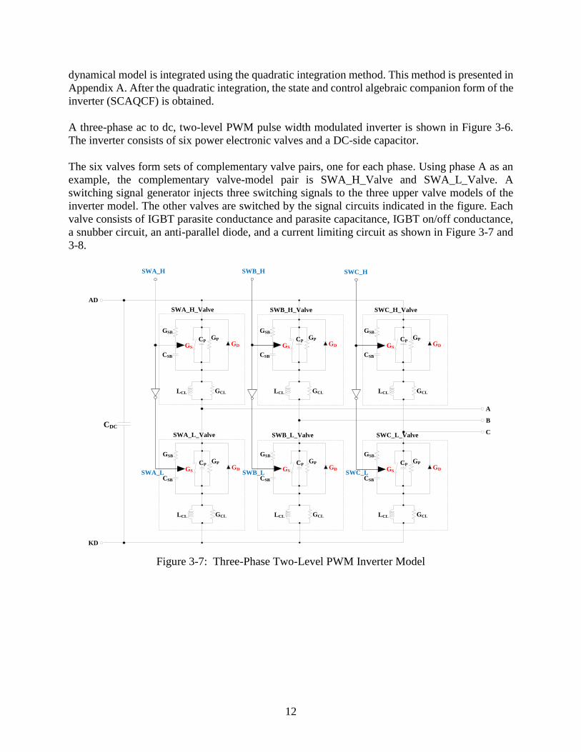
A three-phase ac to dc, two-level PWM pulse width modulated inverter is shown in Figure 3-6.
The inverter consists of six power electronic valves and a DC-side capacitor.
The six valves form sets of complementary valve pairs, one for each phase. Using phase A as an
example, the complementary valve-model pair is SWA_H_Valve and SWA_L_Valve. A
switching signal generator injects three switching signals to the three upper valve models of the
inverter model. The other valves are switched by the signal circuits indicated in the figure. Each
valve consists of IGBT parasite conductance and parasite capacitance, IGBT on/off conductance,
a snubber circuit, an anti-parallel diode, and a current limiting circuit as shown in Figure 3-7 and
3-8.
AD
KD
A
B
CCDC
SWA_H
CSB
GSB
GSGD
CPGP
LCL GCL
SWA_L
SWB_H SWC_H
SWC_LCSB
GSB
GSGD
CPGP
LCL GCL
CSB
GSB
GSGD
CPGP
LCL GCL
CSB
GSB
GSGD
CPGP
LCL GCL
CSB
GSB
GSGD
CPGP
LCL GCL
SWB_L
CSB
GSB
GSGD
CPGP
LCL GCL
SWA_H_Valve
SWA_L_Valve
SWB_H_Valve
SWB_L_Valve
SWC_H_Valve
SWC_L_Valve
Figure 3-7: Three-Phase Two-Level PWM Inverter Model

13
ti
tV
tV
tV
tV
LCL
CP
CSB
2
1
States:
US(t)
Input:
tUS
If (US(t) == 1), GS = GSON
If (US(t) == 0), GS = GSOFF
If (VCP(t) 0), GD = GDOFF
If ( VCP(t) < 0), GD = GDON
IGBT-Conductance Determination
Anti-Parallel-Diode-Conductance Determination
V1(t), i1(t)
CSB
GSB
GSGD
CP
GP
LCL GCL
V2(t), i2(t)
iLCL(t)
+
VCP(t)
-+
VCSB(t)
-
Figure 3-8: Single Valve Model
For each one of the valve states, the dynamic model of the valve has been developed and they are given
in Appendix D. The models are integrated to provide the SCAQCF model for each individual valve. By
combining the valve models, the overall inverter model is obtained.
Note that this model explicitly models the valve operating conditions. Based on the switching signals
or the voltages across the valves, the valve operating condition is determined. This model can capture
whether a valve may mis-operate (mis-fire) because of transients. This is a necessary requirement for a
realistic assessment of the performance of the system under the proposed control schemes.

14
4. Proposed Technologies – Supplementary Predictive Inverter Control
This section presents a methodology for synchronization of CIGs during frequency swings or
disturbances in the system. During these events the frequency if the system oscillates as well the
voltage may experience transients. These transients may cause mis-firings of the inverter power
electronics and may jeopardize the synchronization of the inverter with the system. We propose
supplementary controls of the inverters to anticipate the movement of the system and synchronize
with the transients of the system. The feedback is provided by the dynamic state estimator
discussed in the previous section.
4.1 DSE Enabled Supplementary Predictive Inverter Control
The supplementary predictive inverter control (in P-Q mode or in P-V mode) is achieved by
injection appropriate signals to modulate the switching-signal generator of the inverter. The
supplementary predictive inverter control consists of frequency modulation, modulation index,
phase angle modulation controls as shown in Figure 4-1. This additional control scheme supervises
the inverter controller and guarantees synchronization and stability of the inverter against the
power grid.
Figure 4-1: Block Diagram of the Supplementary Predictive Inverter Control (P-Q Mode)
The supplementary control scheme injects two signals into the inverter controller, as shown in
Figure 4-1. One signal is the target frequency for the operation of the inverter and the other signal
is the target phase angle of the inverter. Both of these signals are computed from the output of the

15
dynamic state estimator. The frequency signal causes a compression or expansion in time of the
switching signal generated by the inverter controller while the phase angle signal cause a
translation in time of the switching sequences generated by the inverter. Both the
compression/expansion and translation in time are applied smoothly causing a gradual shifting
towards the operation of the inverter at the target values. The details of the controls are provided
next.
4.2 Frequency-Modulation Control
In this section, we present the frequency-modulation control. We first need to predict the rates of
phase-angle changes of each CIG system for both the local and the remote sides, as follows:
htt kk 1 (Eq. 4-1)
2
12
12 h
dt
tdfhtft klocal
klocalklocal (Eq. 4-2)
2
12
12 h
dt
tdfhtft kremote
kremotekremote (Eq. 4-3)
Then, we implement a closed-loop feedforward control to generate frequency-modulation control
command as follows: The frequency-modulation control with respect to the one-step forward-
predicted rates of phase angle changes of two CIG systems (feedforward control) is summarized
as follows:
htttttttX klocalkremoteklocalkremoteklocalkremotek 111 (Eq. 4-4)
111
1 kFM
PFM
k
PFM
IFMk tU
KtX
K
KtX (Eq. 4-5)
11 kFMklocalkcntrl tUtftf (Eq. 4-6)
4.3 Modulation-Index and Phase-Angle Modulation Control
In this section, we present the modulation-index and phase-angle modulation controls using real-
and reactive-power references and real- and reactive-power measurements from a digital-signal-
processing (DSP) unit. We provide the modulation parameter for the P-Q control.

16
a. By sending/receiving more reactive power to a power system, we can increase/decrease the
voltage of a power system as described in equation 4-7. Furthermore, we can directly control
the voltage of a converter-interfaced power system by controlling the modulation index m of
the sinusoidal pulse width modulation (SPWM) of the switching-signal generator on behalf of
the inverter control. Therefore, we can control the flow of the reactive power between the
inverter and the power system by controlling the modulation index. Using the relation between
the modulation index and flow of reactive power, we develop the proportional and integral (PI)
control-based reactive-power control as follows:
remotelocalremote
remoteSlocal
V
VXQV
cos
2
(Eq. 4-7)
htQtQtQtQtQtQtX kmkrefkmkrefkmkrefk 1111 (Eq. 4-8)
111
1 kcntrl
PQ
k
PQ
IQ
k tmK
tXK
KtX (Eq. 4-9)
0.10.0 1 kcntrl tm (Eq. 4-10)
b. By controlling the phase angle of the SPWM of the switching-signal generator, we can adjust
the phase-angle difference between an inverter and the power system. Therefore, we can
control the flow of the real power between an inverter and the power system by controlling the
phase angle local of the SPWM as summarized in equation 4-11. For example, by defining the
sinusoidal-reference signal of the phase A of the SPWM as expressed in equation 4-12, we can
increase injection of real power to the power grid by increasing the phase angle, and vice versa.
Using the relation between the phase angle of the SPWM and flow of the real power, we
develop the proportional and integral (PI) real-power control. The real power reference is
determined by the VDC/P droop control.
S
remotelocalremotelocal
X
VVP
sin (Eq. 4-11)
kcntrlkkcntrlkkAref tttftmtS 2cos_ (Eq. 4-12)
SetDCkmDCSetkref VtVkPtP __1 (Eq. 4-13)
htPtPtPtPtPtPtX kmkrefkmkrefkmkrefk 1111 (Eq. 4-14)

17
111
1 kcntrl
PP
k
PP
IPk t
KtX
K
KtX
(Eq. 4-15)
22
1
kcntrl t (Eq. 4-16)
The above referenced target parameters are translated into switching sequence modulation control
as described next.
4.4 Switching-Sequence Modulation Control
In this section, we present the switching-sequence modulation control that generates and controls
switching sequences for the three upper switches of the inverter by using the three control
commands, 1kcntrl tf , 1kcntrl tm , and 1kcntrl t ,obtained from the previous sections. First, we
calculate the initial-operation time for the switching-sequence modulation control using the zero-
crossing time as follows:
0
01
0int2
2
tf
t
tttlocal
V
ZX
(Eq. 4-17)
hkttk int (Eq. 4-18)
Then, we generate base sinusoidal reference signals for the SPWM of the switching-signal
generator based on the base frequency, 60 Hz, as follows:
kbasekkbaseAref tftmtS 2cos__ (Eq. 4-19)
3
22cos__
kbasekkbaseBref tftmtS (Eq. 4-20)
3
42cos__
kbasekkbaseCref tftmtS (Eq. 4-21)
Three-phase base switching sequences for a period expressed in the following equations are based
on the base frequency, 60 Hz, and 1260 Hz of switching frequency. Figures 4-2, 4-3, and 4-4 show
the three-phase base switching sequences for a full period.

18
aaaaaabase ttttttUPSWA 414039210 ,,...,,,,_ (Eq.4-22)
bbbbbbbase ttttttUPSWB 414039210 ,,...,,,,_ (Eq. 4-23)
ccccccbase ttttttUPSWC 414039210 ,,...,,,,_ (Eq. 4-24)
A. Phase-A-Base Switching Sequence
Negative Edge:
20...,,2,1,0,0.1,,2
i
f
iff
f
it
SSN
Sai (Eq. 4-25)
20...,,2,1,0,,22cos,, itbtatfcsolvecbaf baseN (Eq. 4-26)
Positive Edge:
20...,,2,1,0,0.1,,12
i
f
iff
f
it
SSP
Sai (Eq. 4-27)
20...,,2,1,0,,1
22cos,,
it
abtatfcsolvecbaf baseP (Eq. 4-28)
B. Phase-B-Base Switching Sequence
Negative Edge:
20...,,2,1,0,0.1,3
1,2
i
ff
iff
f
it
baseSSN
Sbi (Eq. 4-29)
Positive Edge:
20...,,2,1,0,0.1,3
1,12
i
ff
iff
f
it
baseSSP
Sbi (Eq. 4-30)
C. Phase-C- Base Switching Sequence
Negative Edge:
20...,,2,1,0,0.1,3
2,2
i
ff
iff
f
it
baseSSN
Sci (Eq. 4-31)
Positive Edge:

19
20...,,2,1,0,0.1,3
2,12
i
ff
iff
f
it
baseSSP
Sci (Eq. 4-32)
t0a
t1a
t2a
t3a
t4a
t5a
t6a
t7a
t8a
t9a
t10a
t11a
t12at13a
t14at15a
t16at17a
t18at19a
t20a
t21a
t22a
t23a
t24a
t25a
t26a
t27a
t28a
t29a
t30a
t31a
t32a
t33a
t34a
t35a
t36a
t37a
t38a
t39a
t40a
t41a
Low t
High
Figure 4-2: Base Switching Sequence of the Phase A
t0b
t1b
t2b
t3b
t4b
t5b
t6b
t7b
t8b
t9b
t10b
t11b
t12b
t13b
t14bt15b
t16b
t17b
t18b
t19b
t20b
t21b
t22b
t23b
t24b
t25b
t26b
t27b
t28b
t29b
t30bt31b
t32bt33b
t34bt35b t36b
t37b t38bt39b
t40bt41b
High
Low
Figure 4-3: Base Switching Sequence of the Phase B

20
High
Low
t1c
t2c
t3c
t4c
t5c
t6c
t7c
t8c
t9c
t10c
t11c
t12c
t13c
t14c
t15c
t16c
t17c
t18ct19c
t20c
t21c
t22ct23c
t24ct25c
t26c
t27c
t30c
t31c
t32c
t33c
t34c
t35c
t36c
t37c
t38c
t39c
t40c
t41c
t0c t28c
t29c
Figure 4-4: Base Switching Sequence of the Phase C
By modulating the above base switching sequences with the supplementary predictive inverter
control, the proposed switching-signal generator can control real- and reactive-power flows of the
system as follows:
aaaaaa ctctctctctctUPSWA 414039210 ,,...,,,,_ (Eq. 4-33)
bbbbbb ctctctctctctUPSWB 414039210 ,,...,,,,_ (Eq. 4-34)
cccccc ctctctctctctUPSWC 414039210 ,,...,,,,_ (Eq. 4-35)
A. Phase-A-Modulated Switching Sequence
Negative Edge:
20...,,2,1,0,11
222
i
ffmt
fct
cntrlbasecntrlai
cntrl
cntrlai
(Eq. 4-36)
Positive Edge:
20...,,2,1,0,11
2
12
12
iffm
t
fct
cntrlbasecntrl
ai
cntrl
cntrlai
(Eq. 4-37)
B. Phase-B-Modulated Switching Sequence
Negative Edge:
20...,,2,1,0,11
222
i
ffmt
fct
cntrlbasecntrlbi
cntrl
cntrlbi
(Eq. 4-38)
Positive Edge:

21
20...,,2,1,0,11
2
12
12
iffm
t
fct
cntrlbasecntrl
bi
cntrl
cntrlbi
(Eq. 4-39)
C. Phase-C-Modulated Switching Sequence
Negative Edge:
20...,,2,1,0,11
222
i
ffmt
fct
cntrlbasecntrlci
cntrl
cntrlci
(Eq. 4-40)
Positive Edge:
20...,,2,1,0,11
2
12
12
iffm
t
fct
cntrlbasecntrl
ci
cntrl
cntrlci
(Eq. 4-41)
Figures 4-5, 4-6, and 4-7 show the three-phase modulated switching sequences for a full period.

22
ct0a
ct1a
ct2a
ct3a
ct4a
ct5a
ct6a
ct7a
ct8a
ct9a
ct10a
ct11a
ct12act13a
ct14act15a
ct16act17a
ct18act19a
ct20a
ct21a
ct22a
ct23a
ct24a
ct25a
ct26a
ct27a
ct28a
ct29a
ct30a
ct31a
ct32a
ct33a
ct34a
ct35a
ct36a
ct37a
ct38a
ct39a
ct40a
ct41a
Low t
High
cntrlbasecntrla
cntrl
cntrl
ffmt
f
11
24
cntrlbasecntrl
a
cntrl
cntrl
ffm
t
f
11
2
5
cntrlbasecntrla
cntrl
cntrl
ffmt
f
11
26
cntrlbasecntrl
a
cntrl
cntrl
ffm
t
f
11
2
7
Figure 4-5: Modulated Switching-Signal Sequence of the Phase A (SWA_UP)

23
ct0b
ct1b
ct2b
ct3b
ct4b
ct5b
ct6b
ct7b
ct8b
ct9b
ct10b
ct11b
ct12b
ct13b
ct14bct15b
ct16b
ct17b
ct18b
ct19b
ct20b
ct21b
ct22b
ct23b
ct24b
ct25b
ct26b
ct27b
ct28b
ct29b
ct30bct31b
ct32bct33b
ct34bct35b ct36b
ct37b ct38bct39b
ct40bct41b
High
Low
cntrlbasecntrlb
cntrl
cntrl
ffmt
f
11
24
cntrlbasecntrl
b
cntrl
cntrl
ffm
t
f
11
2
5
cntrlbasecntrlb
cntrl
cntrl
ffmt
f
11
26
cntrlbasecntrl
b
cntrl
cntrl
ffm
t
f
11
2
7
Figure 4-6: Modulated Switching-Signal Sequence of the Phase B (SWB_UP)

24
High
Low
ct1c
ct2c
ct3c
ct4c
ct5c
ct6c
ct7c
ct8c
ct9c
ct10c
ct11c
ct12c
ct13c
ct14c
ct15c
ct16c
ct17c
ct18cct19c
ct20c
ct21c
ct22cct23c
ct24cct25c
ct26c
ct27c
ct30c
ct31c
ct32c
ct33c
ct34c
ct35c
ct36c
ct37c
ct38c
ct39c
ct40c
ct41c
ct0c ct28c
ct29c
cntrlbasecntrlc
cntrl
cntrl
ffmt
f
11
24
cntrlbasecntrl
c
cntrl
cntrl
ffm
t
f
11
2
5
cntrlbasecntrlc
cntrl
cntrl
ffmt
f
11
26
cntrlbasecntrl
c
cntrl
cntrl
ffm
t
f
11
2
7
Figure 4-7: Modulated Switching-Signal Sequence of the Phase C (SWC_UP)

25
5. Simulation Results
In this section we present numerical experiments with the proposed methods to quantify the
performance of the proposed methods.
We present first results of the dynamic state estimator. The numerical experiments have been so
designed as to assess the accuracy by which the dynamic state estimator can determine frequency
and rate of change of frequency of the power grid while it uses local measurements at the inverter
location. The results indicate that the accuracy of the dynamic stat estimator is excellent.
We also present results that quantify the performance of the supplementary inverter controls. The
results indicate that the supplementary inverter controls synchronize the inverter against an
oscillatory power grid and eliminates valve mis-firing during transient periods.
5.1 Performance Evaluation of the Dynamic State Estimator (DSE)
This simulation study evaluates the performance of estimating the frequency and rate of frequency
change locally at the inverter as well as at the system with only local measurements. The simulation
system is provided in Figure 5-1. It consists of a wind turbine system (WTS) which operates at a
speed corresponding at 50 Hz. The WTS is connected to a 34.5kV transmission line via two
converters and a 690V:34.5kV transformer. On the other side, the power grid is assumed to have
a generator that oscillates in such a way that the frequency varies as follows: 60 ± 0.1 Hz. The
source is connected to the power grid via a step up transformer and the 1.5-mile-long line.
34.5kV:115kV690V:34.5kV
WTS
1.5 miles
15kV:115kV
5MW
20MW
50hz, 2.5MVA
G60hz ± 0.1hz,
80MVA
Local
Side
Remote
Side
Figure 5-1: Simulation System for Frequency Estimation
One of the objectives of the dynamic state estimator is to provide the best estimate of the frequency
and the rate of frequency change at the local (inverter location) and remote side (34.5kV/115kV
transformer). Numerical experiments have been performed with different lengths of lines.

26
Figure 5-2 shows the results of the frequency and rate of frequency change, at the local side
(inverter side) of the 34.5kV transmission line. The line is 1.5 miles-long. The first two channels
show instantaneous values of three phase measured and DSE estimated voltages. The third and
fourth channel shows the actual and estimated frequency and the forth channel shows the error
(difference). We observe that the maximum absolute error is quite small (18.87 μHz). The fifth
channel shows the actual and estimated rate of frequency change and the sixth channel shows the
error (difference). The error of the estimated rate of frequency change is very small (0.124 mHz/s).
Figure 5-2: Simulation Results, 1.5-Mile Line, Local Side
27.80 kV
-27.80 kV
Actual_Voltage_PhaseA_Side1 (V)
Actual_Voltage_PhaseB_Side1 (V)
Actual_Voltage_PhaseC_Side1 (V)
27.80 kV
-27.80 kV
DSEOutput_Voltage_PhaseA_Side1 (V)
DSEOutput_Voltage_PhaseB_Side1 (V)
DSEOutput_Voltage_PhaseC_Side1 (V)
60.09 Hz
59.98 Hz
Actual_Freq_Side1 (Hz)
Estimated_Freq_Side1 (Hz)
18.27 uHz
-18.87 uHz
Freq_Error_Side1 (Hz)
0.581 Hz/s
-0.580 Hz/s
Actual_dfdt_Side1 (Hz/s)
Estimated_dfdt_Side1 (Hz/s)
-2.602 uHz/s
-0.124 mHz/s
Error_dfdt_Side1 (Hz/s)
0.600 s 1.101 s

27
Figure 5-3 shows the results of the frequency and rate of frequency change, at the remote side of
the 34.5kV transmission line. The line is 1.5 miles-long. The first two channels show instantaneous
values of three phase measured and DSE estimated voltages. The third and fourth channel shows
the actual and estimated frequency and the forth channel shows the error (difference). We observe
that the maximum absolute error is quite small (0.177 mHz). The fifth channel shows the actual
and estimated rate of frequency change and the sixth channel shows the error (difference). The
error of the estimated rate of frequency change is very small (1.144 mHz/s).
Figure 5-3: Simulation Results, 1.5-Mile Line, Remote Side
27.79 kV
-27.79 kV
Actual_Voltage_PhaseA_Side2 (V)
Actual_Voltage_PhaseB_Side2 (V)
Actual_Voltage_PhaseC_Side2 (V)
27.79 kV
-27.79 kV
DSEOutput_Voltage_PhaseA_Side2 (V)
DSEOutput_Voltage_PhaseB_Side2 (V)
DSEOutput_Voltage_PhaseC_Side2 (V)
60.09 Hz
59.98 Hz
Actual_Freq_Side2 (Hz)
Estimated_Freq_Side2 (Hz)
0.177 mHz
-65.13 uHz
Freq_Error_Side2 (Hz)
0.589 Hz/s
-0.588 Hz/s
Actual_dfdt_Side2 (Hz/s)
Estimated_dfdt_Side2 (Hz/s)
1.049 mHz/s
-1.144 mHz/s
Error_dfdt_Side2 (Hz/s)
0.600 s 1.101 s
28
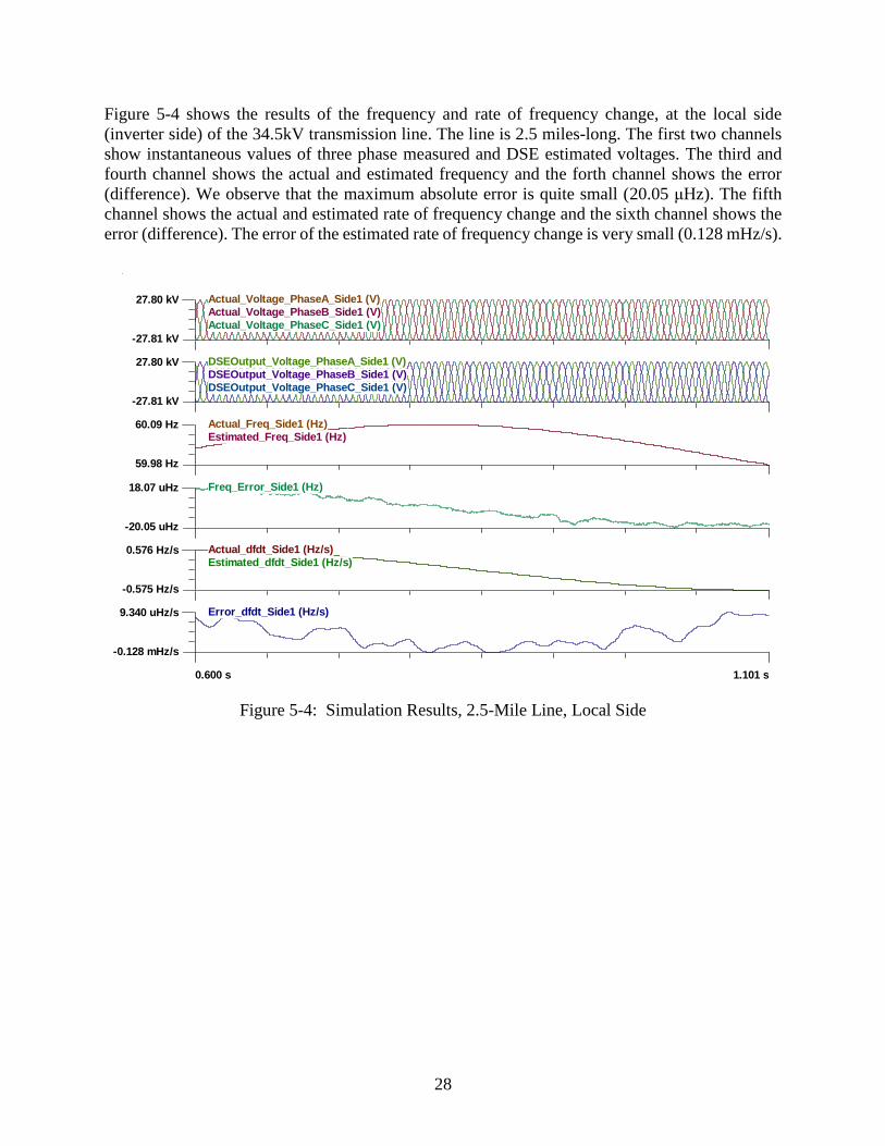
Figure 5-4 shows the results of the frequency and rate of frequency change, at the local side
(inverter side) of the 34.5kV transmission line. The line is 2.5 miles-long. The first two channels
show instantaneous values of three phase measured and DSE estimated voltages. The third and
fourth channel shows the actual and estimated frequency and the forth channel shows the error
(difference). We observe that the maximum absolute error is quite small (20.05 μHz). The fifth
channel shows the actual and estimated rate of frequency change and the sixth channel shows the
error (difference). The error of the estimated rate of frequency change is very small (0.128 mHz/s).
Figure 5-4: Simulation Results, 2.5-Mile Line, Local Side
27.80 kV
-27.81 kV
Actual_Voltage_PhaseA_Side1 (V)
Actual_Voltage_PhaseB_Side1 (V)
Actual_Voltage_PhaseC_Side1 (V)
27.80 kV
-27.81 kV
DSEOutput_Voltage_PhaseA_Side1 (V)
DSEOutput_Voltage_PhaseB_Side1 (V)
DSEOutput_Voltage_PhaseC_Side1 (V)
60.09 Hz
59.98 Hz
Actual_Freq_Side1 (Hz)
Estimated_Freq_Side1 (Hz)
18.07 uHz
-20.05 uHz
Freq_Error_Side1 (Hz)
0.576 Hz/s
-0.575 Hz/s
Actual_dfdt_Side1 (Hz/s)
Estimated_dfdt_Side1 (Hz/s)
9.340 uHz/s
-0.128 mHz/s
Error_dfdt_Side1 (Hz/s)
0.600 s 1.101 s

29
Figure 5-5 shows the results of the frequency and rate of frequency change, at the remote side of
the 34.5kV transmission line. The line is 2.5 miles-long. The first two channels show instantaneous
values of three phase measured and DSE estimated voltages. The third and fourth channel shows
the actual and estimated frequency and the forth channel shows the error (difference). We observe
that the maximum absolute error is quite small (0.282 mHz). The fifth channel shows the actual
and estimated rate of frequency change and the sixth channel shows the error (difference). The
error of the estimated rate of frequency change is very small (1.906 mHz/s).
Figure 5-5: Simulation Results, 2.5-Mile-Line, Remote Side
27.79 kV
-27.79 kV
Actual_Voltage_PhaseA_Side2 (V)
Actual_Voltage_PhaseB_Side2 (V)
Actual_Voltage_PhaseC_Side2 (V)
27.79 kV
-27.79 kV
DSEOutput_Voltage_PhaseA_Side2 (V)
DSEOutput_Voltage_PhaseB_Side2 (V)
DSEOutput_Voltage_PhaseC_Side2 (V)
60.09 Hz
59.97 Hz
Actual_Freq_Side2 (Hz)
Estimated_Freq_Side2 (Hz)
0.282 mHz
-94.64 uHz
Freq_Error_Side2 (Hz)
0.589 Hz/s
-0.588 Hz/s
Actual_dfdt_Side2 (Hz/s)
Estimated_dfdt_Side2 (Hz/s)
1.689 mHz/s
-1.906 mHz/s
Error_dfdt_Side2 (Hz/s)
0.600 s 1.101 s

30
Figure 5-6 shows the results of the frequency and rate of frequency change, at the local side
(inverter side) of the 34.5kV transmission line. The line is 4.0 miles-long. The first two channels
show instantaneous values of three phase measured and DSE estimated voltages. The third and
fourth channel shows the actual and estimated frequency and the forth channel shows the error
(difference). We observe that the maximum absolute error is quite small (18.53 μHz). The fifth
channel shows the actual and estimated rate of frequency change and the sixth channel shows the
error (difference). The error of the estimated rate of frequency change is very small (0.135 mHz/s).
Figure 5-6: Simulation Results, 4-Mile Line, Local Side
27.81 kV
-27.81 kV
Actual_Voltage_PhaseA_Side1 (V)
Actual_Voltage_PhaseB_Side1 (V)
Actual_Voltage_PhaseC_Side1 (V)
27.81 kV
-27.81 kV
DSEOutput_Voltage_PhaseA_Side1 (V)
DSEOutput_Voltage_PhaseB_Side1 (V)
DSEOutput_Voltage_PhaseC_Side1 (V)
60.09 Hz
59.98 Hz
Actual_Freq_Side1 (Hz)
Estimated_Freq_Side1 (Hz)
18.03 uHz
-18.53 uHz
Freq_Error_Side1 (Hz)
0.569 Hz/s
-0.568 Hz/s
Actual_dfdt_Side1 (Hz/s)
Estimated_dfdt_Side1 (Hz/s)
4.507 uHz/s
-0.135 mHz/s
Error_dfdt_Side1 (Hz/s)
0.600 s 1.100 s

31
Figure 5-7 shows the results of the frequency and rate of frequency change, at the remote side of
the 34.5kV transmission line. The line is 4.0 miles-long. The first two channels show instantaneous
values of three phase measured and DSE estimated voltages. The third and fourth channel shows
the actual and estimated frequency and the forth channel shows the error (difference). We observe
that the maximum absolute error is quite small (0.451 mHz). The fifth channel shows the actual
and estimated rate of frequency change and the sixth channel shows the error (difference). The
error of the estimated rate of frequency change is very small (2.896 mHz/s).
Figure 5-7: Simulation Results, 4-Mile Line, Remote Side
27.79 kV
-27.79 kV
Actual_Voltage_PhaseA_Side2 (V)
Actual_Voltage_PhaseB_Side2 (V)
Actual_Voltage_PhaseC_Side2 (V)
27.79 kV
-27.80 kV
DSEOutput_Voltage_PhaseA_Side2 (V)
DSEOutput_Voltage_PhaseB_Side2 (V)
DSEOutput_Voltage_PhaseC_Side2 (V)
60.09 Hz
59.98 Hz
Actual_Freq_Side2 (Hz)
Estimated_Freq_Side2 (Hz)
0.451 mHz
-0.129 mHz
Freq_Error_Side2 (Hz)
0.589 Hz/s
-0.588 Hz/s
Actual_dfdt_Side2 (Hz/s)
Estimated_dfdt_Side2 (Hz/s)
2.751 mHz/s
-2.896 mHz/s
Error_dfdt_Side2 (Hz/s)
0.600 s 1.100 s

32
All results are summarized in the Tables 5-1 and 5-2. The frequency varies from 59.98~60.09 Hz,
and the rate of frequency change varies from -0.6 ~ 0.6 Hz/s. From the two tables below, the
maximum absolute error is within 0.001% for frequency and 0.5% for rate of frequency change.
We can conclude that the proposed method can accurately estimate the local and remote side
frequency as well as rate of frequency change with local information only.
Table 5-1: Results of Side 1
Case Number Line length Frequency Error dFreq/dt error
1 1.5 miles -1.887×10⁻⁵ ~ 1.827×10⁻⁵ Hz -1.24×10⁻⁴ ~ -2.602×10⁻⁶ Hz/s
2 2.5 miles -2.005×10⁻⁵ ~ 1.807×10⁻⁵ Hz -1.28×10⁻⁴ ~ 9.340×10⁻⁶ Hz/s
3 4 miles -1.853×10⁻⁵ ~ 1.803×10⁻⁵ Hz -1.35×10⁻⁴ ~ 4.507×10⁻⁶ Hz/s
Table 5-2: Results of Side 2
Case Number Line length Frequency Error dFreq/dt error
1 1.5 miles -6.513×10⁻⁵ ~ 1.77×10⁻⁴ Hz -1.144×10⁻³ ~ 1.049×10⁻³ Hz/s
2 2.5 miles -9.464×10⁻⁵ ~ 2.82×10⁻⁴ Hz -1.906×10⁻³ ~ 1.689×10⁻³ Hz/s
3 4 miles -1.29×10⁻⁴ ~ 4.51×10⁻⁴ Hz -2.896×10⁻³ ~ 2.751×10⁻³ Hz/s

33
5.2 Performance Evaluation of the Supplementary Predictive Inverter Control Enabled
by Dynamic State Estimator (DSE)
Numerical experiments were carried out to evaluate the performance of the supplementary
predictive inverter control. For each numerical experiment two scenarios were investigated:
scenario 1: the proposed supplementary control is disabled and scenario 2: the proposed
supplementary control is enabled while keeping the system conditions the same (same set of
disturbances).
The numerical experiments were performed using the test system of Figure 5-8. The system
consists of a type 4 wind turbine system connected to a step up transformer, a 35 kV transmission
circuit, connecting to a collector substation. Part of the power grid beyond the collector substation
is shown in Figure 5-8. A number of key components of this system are listed in Table 5-3.
Numerical experiments with this system, by enabling the supplementary inverter control indicate
that the proposed control practically eliminates valve mis-operations in the inverter when
disturbances occur in the system. We present two example cases in the following subsections.
DC ACA B C
Switching-Signal Generator
DC ACA B C
Switching-Signal Generator
VF-G
1 2
DSP IIStart... DSP II
Start...
DSP IIStart...
1 2
12
VF-G
DSE
BLPI-35TR
BLPO-35TR
BRPI-35TR
BRPO-35TR
IDFS1
IDFS2
IFS1IFS2
II1MAG1
II1TH1
INV-S
WAUP
INV-S
WBUP
INV-S
WCUP
IP1 IQ1
IV1MAG1
IV1TH1
NULL3
NULL4
NULL5
NULL6
NULL7
NULL8
NULL9
OUTAM1
OUTVOLT1
OUTVOLT2
PI-SG
RCT-SW
AUP
RCT-SW
BUP
RCT-SW
CUP
RDFSRDFS2
RFSRFS2
RI1MAG
RI1TH
RP RQRV1TH
TR1-L1L
TR1-L1R
VACFG1
VDCMAG
WTS-AC
WTS-ACF
WTS-ACFA
WTS-DC
WTS-S
WTS-TR
ZXINV
ZXRCT
1
2 3
4 5
6
7
8
910
11
12
13
14
15
16
17
Figure 5-8: Test Bed for the Supplementary Predictive Inverter Control

34
Table 5-3: List of the Components of the Test Bed
Index Component
1 Variable-Speed Wind Turbine (0.690 kV / 2.5 MVA )
2 Wind Turbine-Side Converter (0.690 kV / 2.5 MVA)
3 Grid-Side Inverter (0.690 kV / 2.5 MVA)
4 Wind Turbine-Side Converter Controller
5 Grid-Side Inverter Controller
6 Digital Signal Processor (DSP) for Wind Turbine-Side Converter Control
7 DSPs for Grid-Side Inverter Control
8 Dynamic State Estimator (DSE)
9 L-C Filter
10 Delta-Wye Transformer (0.670 kV / 34.5 kV)
11 1.5-Mile Transmission Line (34.5 kV)
12 Wye-Wye Transformer (34.5 kV / 115 kV)
13 Three-Phase Load (34.5 kV / 5 MVA)
14 1.5-Mile Transmission Line (115 kV)
15 Three-Phase Load (115 kV / 20 MVA)
16 Wye-Delta Transformer (115 kV / 15 kV)
17 Variable-Frequency Three-Phase Equivalent Voltage Source (15 kV / 80 MVA)

35
5.2.1 Case 1: WTS Performance Without Proposed Control Strategy
The system of Figure 5-8 was simulated under the following event: first, the grid-side inverter
operates under its own controller. The wind power results in rotor speed corresponding to 50 Hz
and the wind has a 10% variability. The power grid experiences an oscillation. At the remote
generator, the frequency oscillation is tHz 2sin1.060 Hz. The grid-side inverter control is set
to operate at 2 MW/0.8 kVDC and 0.5 MVar (P-Q control). Any power imbalances in the system
are absorbed by the conventional generation.
Simulation results are shown in Figure 5-9 over a period of 4 seconds. The first two traces show
the voltages and currents at the output of the inverter. Traces 3 and 4 show the real and reactive
power output of the inverter. Note the variability caused by the oscillating conditions of the power
grid. Traces 5 show the local and remote phase angles of the phase A voltage at these locations.
Traces 6 show the local and remote frequency. Note a small oscillation of frequency across the
connecting transmission line. The last trace shows the dc voltage at the inverter input. The
transients are caused by the oscillating frequency of the system and involve occasional mis-
operation of the valves, not shown in the graphs.
Figure 5-9: Simulation Result when the Proposed Control Is Disabled
27.90 kV
-27.90 kV
WTSAC_VAN (V)
WTSAC_VBN (V)
WTSAC_VCN (V)
58.20 A
-60.02 A
WTSAC_IA (A)
WTSAC_IB (A)
WTSAC_IC (A)
2145.2 kW
1832.6 kW
Real_Power (kW)
539.1 kVar
334.5 kVar
Reactive_Power (kVar)
1.307 rad
0.156 rad
TH_Local (rad)
TH_Remote (rad)
60.11 Hz
59.89 Hz
FQ_Local (Hz)
FQ_remote_ (Hz)
828.5 V
792.1 V
VDC (V)
0.380 s 4.001 s

36
5.2.2 Case 2: WTS Performance With Proposed Control Strategy
The system of Figure 5-8 was simulated under the following event: first, the grid-side inverter
operates with the supplementary control which injects additional signal to the inverter controller.
The wind power results in rotor speed corresponding to 50 Hz and the wind has a 10% variability.
The power grid experiences an oscillation. At the remote generator, the frequency oscillation is
tHz 2sin1.060 Hz. The grid-side inverter control is set to operate at 2 MW/0.8 kVDC and 0.5
MVar (P-Q control). Any power imbalances in the system are absorbed by the conventional
generation.
Simulation results are shown in Figure 5-10 over a period of 4 seconds. The first two traces show
the voltages and currents at the output of the inverter. Traces 3 and 4 show the real and reactive
power output of the inverter. Note that the real and reactive power is almost constant, less than 2%
variation. Traces 5 show the local and remote phase angles of the phase A voltage at these locations
– the difference is controlled to a constant value. Traces 6 show the local and remote frequency.
Note the frequency difference across the connecting transmission line is practically zero. The last
trace shows the dc voltage at the inverter input. The WTS “follows” and “synchronizes” with the
power grid almost perfectly. No valve mis-operations were detected in this case.
Figure 5-10: Simulation Results when the Proposed Control is Enabled
27.91 kV
-27.90 kV
WTSAC_VAN (V)
WTSAC_VBN (V)
WTSAC_VCN (V)
60.12 A
-57.79 A
WTSAC_IA (A)
WTSAC_IB (A)
WTSAC_IC (A)
2094.0 kW
1917.3 kW
Real Power (kW)
540.3 kVar
435.3 kVar
Reactive Power (kVar)
1.294 rad
0.209 rad
TH_Local (rad)
TH_Remote (rad)
60.11 Hz
59.89 Hz
FQ_Local (Hz)
FQ_remote (Hz)
831.2 V
795.4 V
VDC (V)
0.349 s 4.000 s

37
6. Conclusions and Future Work
This study investigated the issues generated from high penetration of converter-interfaced
generation (CIGs) in the power grid. The following issues have been identified:
1. As CIGs are becoming a larger portion of the power grid generation, the fault current levels
decrease, causing protection gaps.
2. Present day low voltage ride through strategies will cause severe problems in a system with
high penetration CIGs as a disturbance may cause a large number of CIGs to temporarily
shut down in ride through mode. While a small number of CIGs may be absorbed by the
system, a large number (or a large proportion of the generation going into ride through
mode) may result in no recovery of the system. This is unknown territory.
3. Disturbances may cause valve mis-operation in inverter systems and subsequent transients
and/or oscillations among the various inverters of the system.
To address these issues, we proposed new methods for protection which do not depend on the fault
current level. This protection approach is based on dynamic state estimation methods. To address
the issue of stabilizing and synchronizing CIGs with the power grid we proposed and tested the
use of dynamic state estimation to provide signal to the inverter controller for supplementary
inverter control. The results show that the inverter is synchronized with the power grid under
disturbances that may occur remotely from the CIG inverter. This method is very promising as it
also eliminates oscillation between CIGs as well.
The application of the proposed method requires an infrastructure that enables dynamic state
estimation at each CIG. The technology exists today to provide the required measurements and at
the required speeds to perform dynamic state estimation. In essence the method provides full state
feedback for the control of the CIGs. While in this project we experimented with one type of
supplementary control, the ability to provide full state feedback via the dynamic state estimation
opens up the ability to use more sophisticated control methodologies. Future work should focus
on utilizing the dynamic state estimation to provide full state feedback and investigate additional
control methods. The methods should be integrated with resource management, for example
managing the available wind energy (in case of a WTS) or the PV energy, especially in cases that
there is some amount of local storage. The dynamic stat estimation based protection, should be
integrated in such a system.

38
7. Publications as Direct Result of this Project
Technical Papers
[1] Liu, Yu; Sakis A.P. Meliopoulos, Rui Fan, and Liangyi Sun. "Dynamic State Estimation
Based Protection of Microgrid Circuits," Proceedings of the IEEE-PES 2015 General
Meeting, Denver, CO, July 26-30, 2015.
[2] Liu, Yu; Sanghun Choi, Sakis Meliopoulos, Rui Fan, Liangyi Sun, and Zhenyu Tan.
“Dynamic State Estimation Enabled Predictive Inverter Control”, Accepted, Proceedings of
the IEEE-PES 2016 General Meeting, Boston, MA, July 17-21, 2016.
ECE Master Thesis
[1] Weldy, Christopher. Master Thesis “Stability of a 24-Bus Power System with Converter
Interfaced Generation” Georgia Institute of Technology, 2015.

39
8. References
[0] Ackermann, Thomas; Editor. Wind Power in Power Systems, John Wiley and Sons, Ltd,
second edition, 2012.
[1] Blaabjerg, Frede; and Ke Ma. “Future on Power Electronics for Wind Turbine Systems,” in
IEEE Journal of Emerging and Selected topics in Power Electronics, vol. 1, no. 3, pp.139-
152, September 2013.
[2] Li, C.; P. Zhan, J. Wen, M. Yao, N. Li and W. J. Lee. “Offshore Wind Farm Integration
and Frequency Support Control Utilizing Hybrid Multi-terminal HVDC Transmission,” in
IEEE Transactions on Industry Applications, vol. 50, no. 4, pp. 2788-2797, July/August
2009.
[3] Miao, L.; J. Wen, H. Xie, C. Yue and W. J. Lee. “Coordinated Control Strategy of Wind
Turbine Generator and Energy Storage Equipment for Frequency Support,” in IEEE
Transactions on Industry Applications, vol. 51, no. 4, pp 2732-2742, July/August 2015.
[4] Gowaid, I. A.; A. EI-Zawawi, and M. EI-Gammal. “Improved inertia and frequency
support from grid-connected DFIG wind farms,” in Proceeding of IEEE PES Power System
Conference Exposition, pp. 1-9. 2011.
[5] Gonzalez-Longatt, F.M. “Activation Schemes of Synthetic Inertia Controller on Full
Converter Wind Turbine (Type 4)”, in 2015 IEEE Power and Energy Society General
Meeting (PES 2015), pp. 1-5, July 26-30, 2015.
[6] Lalor, G.; A. Mullane, and M. O’Malley. “Frequency Control and Wind Turbine
Technologies,” in IEEE Transactions on Power System, vol. 20, no. 4, pp. 1905-1913,
November 2005.
[7] Arani, M. F. M.; and E. F. El-Saadany. “Implementing virtual inertia in DFIG-based wind
power generation,” in IEEE Transactions on Power System, vol. 28, no. 2, pp. 1373-1384,
June 2013.
[8] Baran, M. E.; and N. R. Mahajan. “Overcurrent Protection on Voltage-Source-Converter-
Based Multi-terminal DC Distribution Systems,” in IEEE Transactions on Power Delivery,
vol. 22, no. 1, pp. 406-412, January 2007.
[9] Kamwa, I.; R. Grondin, and Y. Hebert. “Wide-Area Measurement Based Stabilizing
Control of Large Power Systems-A Decentralized/Hierarchical Approach,” in IEEE
Transactions on Power Systems, vol. 16, no. 1, pp. 136-153, February 2001.
[10] Fang, Xi; Satyajayant Misra, Guoliang Xue, and Dejun Yang. “Smart Grid - The New and
Improved Power Grid: A Survey,” in IEEE Communications Survey & Tutorials, vol. 14,
no. 4, pp. 944-980, December 2011.
[11] Mitter, C. S.; A. R. Hefner, D. Y. Chen, and F. C. Lee. “Insulated Gate Bipolar Transistor
(IGBT) Modeling using IG-SPICE,” in IEEE Trans. on Industry Applications, vol. 30, no.
1, pp. 24-33, August 2002.
[12] Hefner, A. R. “A Dynamic Electro-Thermal Model for IGBT,” in IEEE Trans. on Industry
Applications, vol. 30, no. 2, pp. 394-405, August 2002.
[13] Hefner, A. R. “Modeling Power Semiconductor Devices for Realistic Simulation,” in IEEE
4th Workshop on Computers in Power Electronics, pp. 11-44, August 1994.

40
[14] Kuang, S.; B. W. Williams, and S. J. Finney. “A Review of IGBT Models,” in IEEE Trans.
on Power Electronics, vol. 15, no. 6, pp. 1250-1266, August 2002.
[15] Biswas, S. K.; B. Basak, and K. S. Rajashekara. “A Review of IGBT Models,” in IEEE
Industry Applications Society Annual Meeting, vol. 2, pp. 1483-1489, September 1991.
[16] Dommel, H. W. “Digital Computer Solution of Electromagnetic Transients in Single-and
Multiphase Networks,” in IEEE Transactions on Power Apparatus and Systems, no. 4, pp.
388-399, January 2007.
[17] Johnson, R. B. I.; B. J. Cory, and M. J. Short. “A Tunable Integration Method for the
Simulator of Power System Dynamics,” in IEEE Transactions on Power Systems, vol. 3,
no. 4, pp. 1530-1537, August 2002.
[18] Yen, K. K.; Z. Hu, and J. Andrian. “Stability Study of Parallel Predictor-Corrector
Numerical Integration Algorithms and Redesign,” in IEEE Proceedings Energy and
Information Technologies in the Southeast, vol. 2, pp. 417-420, April 1989.
[19] Van Den Bosch, P. P. J.; and H. R. Visser. “Simulation of State-Events in Power Electronic
Devices,” in Fourth International Conference on Power Electronics and Variable-Speed
Drives, IEEE Proceedings Energy and Information Technologies in the Southeast, pp. 184-
189, 1990.
[20] Kato, T.; and K. Ikeuchi. “Variable Order and Variable Step-Size Integration Method for
Transient Analysis Programs,” in IEEE Transactions on Power Systems, vol. 6, no. 1, pp.
206-213, August 2002.
[21] Kato, T.; and T. Kataoka. “Computer-Aided Analysis of a Power Electronic Circuit by a
New Multi-rate Method,” in IEEE Power Electronics Specialist Conference, vol. 2, pp.
1076-1083, May 1998.
[22] Takano, H.; S. M. Ulhaq, and M. Nakaoka. “Computer-aided simulation technique of
digitally controlled switched-mode power conversion circuits and systems using state
variable matrices,” in IEEE Proceedings of the Power Conversion Conference, vol. 1, pp.
411-418, August 1997.
[23] Pejovic, P.; and D. Maksimovic. “PETs-a Simulation Tool for Power Electronics,” in IEEE
Workshop on Computers in Power Electronics, pp. 1-8, August 1996.
[24] Dinavahi, V. R.; M. R. Iravani, and R. Boner. “Real-Time Digital Simulation of Power
Electronic Apparatus Interfaced With Digital Controllers,” in IEEE Transactions on Power
Delivery, vol. 16, no. 4, pp. 775-781, August 2002.
[25] Blaabjerg, F.; R. Teodorescu, M. Liserre, and A. V. Timbus. “Overview of Control and
Grid Synchronization for Distributed Power Generation Systems,” in IEEE Transactions on
Industrial Electronics, vol. 53, no. 5, pp. 1398-1409, October 2006.
[26] Saccomando, G.; and J. Svensson. “Transient operation of grid-connected voltage source
converter under unbalanced voltage conditions,” in IEEE Thirty-Sixth IAS Annual Meeting
Conference, vol. 4, pp. 2419-2424, September 2001.
[27] Agirman, I.; and V. Blasko. “A Novel Control Method of a VSC without AC Line Voltage
Sensors,” in IEEE Transactions on Industry Applications, vol. 39, no. 2, pp. 519-524,
March 2003.

41
[28] Teodorescu, R.; and F. Blaabjerg. “Flexible Control of Small Wind Turbines With Grid
Failure Detection Operating in Stand-Alone and Grid-Connected Mode,” in IEEE
Transactions on Power Electronics, vol. 19, no. 5, pp. 1323-1332, September 2004.
[29] Teodorescu, R.; F. Blaabjerg, U. Borup, and M. Liserre. “A New Control Structure for
Grid-Connected LCL PV Inverters with Zero Steady-State Error and Selective Harmonic
Compensation,” in IEEE Applied Power Electronics Conference and Exposition 2004, vol.
1, pp. 580-586, 2004.
[30] Song, S.; S. Kang, and N. Hahm. “Implementation and control of grid connected AC-DC-
AC power converter for variable speed wind energy conversion system,” in IEEE Applied
Power Electronics Conference and Exposition 2004, vol. 1, pp. 154-158, 2003.
[31] Zhu, H.; B. Arnet, L. Haines, E. Shaffer, and J. Lai. “Grid Synchronization Control without
AC Voltage Sensors,” in IEEE Applied Power Electronics Conference and Exposition
2003, vol. 1, pp. 172-178, 2003.
[32] Ramos, C. J.; A. P. Martins, A. S. Araujo, and A. S. Carvalho. “Current Control in the Grid
Connection of the Double-Output Induction Generator Linked to a Variable Speed Wind
Turbine,” in IEEE 2002 Annual Conference of Industrial Electronics Society, vol. 2, pp.
979-984, 2002.
[33] Candusso, D.; I. Valero, and A. Walter. “Modelling, Control and Simulation of a Fuel Cell
Based Power Supply System with Energy Management,” in IEEE 2002 Annual Conference
of Industrial Electronics Society, vol. 2, pp. 1294-1299, 2002.
[34] Teodorescu, R.; F. Iov, and F. Walter. “Flexible Development and Test Systems for 11 kW
Wind Turbine,” in IEEE 34th Annual Power Electronics Specialist Conference, vol. 1, pp.
67-72, June 2003.
[35] Twining, E.; and D. G. Holmes. “Grid Current Regulation of a Three-Phase Voltage Source
Inverter With an LCL Input Filter,” in IEEE Transactions on Power Electronics, vol. 18,
no. 3, pp. 888-895, May 2003.
[36] Fukuda, S.; and T. Yoda. “A Novel Current-Tracking Method for Active Filters Based on a
Sinusoidal Internal Model,” in IEEE Transactions on Industrial Applications, vol. 37, no.
3, pp. 888-895, May 2001.
[37] Zmood, D. N.; and D. G. Homes. “Stationary Frame Current Regulation of PWM Inverters
with Zero Steday-State Error,” in IEEE Trans. on Power Electronics, vol. 18, no. 3, pp.
814-822, May 2003.
[38] Ciobotaru, M.; R. Teodorescu, and F. Blaabjerg. “Control of Single-Stage Single-phase PV
Inverter,” in 2005 European Conference on Power Electronics and Applications, pp. 1-10,
2005.
[39] Malesani, L.; and P. Tenti. “A Novel Hysteresis Control Method for Current-Controlled
Voltage-Source PWM Inverters with Constant Modulation Frequency,” in IEEE
Transactions on Industrial Applications, pp. 88-92, February 1990.
[40] Meliopoulos, Sakis A.P.; G. J. Cokkinides, and G. K. Stefopoulos. “Quadratic Integration
Method,” presented at the International Conference on Power Systems Transients (IPST
2015), Paper No. IPST05 - 231, June 15-18, 2005.
[41] Arrillaga, J.; M. H. J. Bollen, and N.R. Watson. “Power Quality Following Deregulation,”
in Proceedings of the IEEE, vol. 88, no. 2, pp. 246-261, February 2000.

42
[42] Novosel, D.; V. Madani, B. Bhargave, Vu. Khoi, and J. Cole. “Dawn of the Grid
Synchronization,” in IEEE Power and Energy Magazine, vol. 6, no. 1, pp. 49-60, February
2008.
[43] Gungor, V. C.; D. Sahin, T. Kocak, S. Ergut, C. Buccella, C. Cecati, and G. P. Hancke. “A
Survey on Smart Grid Potential Applications and Communication Requirements,” in IEEE
Transactions on Industrial Informatics, vol. 9, no. 1, pp. 28-42, September 2012.
[44] Agrawal, G. P. Fiber-Optic Communication Systems, John Wiley & Sons, 2002.
[45] Kamwa, I.; S. R. Samantaray, and G. Joos. “Wide Frequency Range Adaptive Phasor and
Frequency PMU Algorithms,” in IEEE Transactions on Smart Grid, vol. 5, no. 2, pp. 569-
579, February 2014.
[46] Romano, P.; and M. Paolone. “Enhanced Interpolated-DFT for Synchrophasor Estimation
in FPGAs: Theory, Implementation, and Validation of a PMU Prototype,” in IEEE
Transactions on Instrumentation and Measurement, vol. 63, no. 12, pp. 2824-2836,
November 2014.
[47] Kamwa, I.; S. R. Samantaray, and G. Joos. “Compliance Analysis of PMU Algorithms and
Devices for Wide-Area Stabilizing Control of Large Power Systems,” in IEEE
Transactions on Power Systems, vol. 28, no. 2, pp. 1766-1778, April 2013.
[48] Chen, C. “A Two-Stage Solution Procedure for Digital Power Metering According to IEEE
Standard 1459-2010 in Single-Phase System,” in IEEE Transactions on Industrial
Electronics, vol. 60, no. 12, pp. 5550-5557, June 2013.

43
9. Appendix A: The Quadratic Integration Method
This section presents the description of the quadratic integration. The quadratic integration starts
from the dynamic model of a component. We refer to this as the compact model. Then, the
quadratic integration method consists of two consecutive steps [40].
First, the nonlinear differential equations of the compact model of an actual device are
reformulated to fully equivalent quadratic equations by introducing additional states and algebraic
equations if the nonlinear differential equations have higher-order terms than the second degree.
The procedure results in the following quadratized device model:
1 1 1 1
2 2 2 2
3 3 3 3 3 3
( )( ) ( ) ( )
( )0 ( ) ( )
0 ( ) ( ) ( ) ( ) ( ) ( ) ( ) ( )
eqx equ eqxd eqc
eqx equ eqxd eqc
T i T i T i
eqx equ eqxx equu equx feqc
d ti t Y t Y t D C
dt
d tY t Y t D C
dt
Y t Y t t F t t F t t F t C
xx u
xx u
x u x x u u u x
(Eq. A-1)
Second, the quadratized model from the first step is integrated using an implicit numerical scheme
assuming that the states of the quadratized model vary quadratically within a time step h. This
assumption is shown in Figure A-1.
Figure A-1: Illustration of the Quadratic Integration Method

44
The quadratic integration method is applied to every set of equations separately in the quadratized
device model. Since there are three sets of equations, each one is analyzed below to show how
they can be transferred to State and Control Algebraic Quadratic Companion Form (SCAQCF).
The model is obtained for a given time step h as follows:
1) Through variable equations:
1 1 1 1
( )( ) ( ) ( )eqx equ eqxd eqc
d ti t Y t Y t D C
dt
xx u
After applying quadratic integration, we have
From time t-h to t,
1 1 1 1 1 1 1
4 8 4( ) ( ) ( ) ( ) ( ) ( ) ( ) ( ) ( )eqxd eqx equ eqxd m eqxd eqx equi t D Y t Y t D t D Y t h i t h Y t h
h h h x u x x u
From time t-h to tm,
1 1 1 1 1 1 1 1
1 2 1 5 1 1 3( ) ( ) ( ) ( ) ( ) ( ) ( ) ( ) ( )
2 2 2 2 2 2m eqxd eqxd eqx m equ m eqx eqxd equ eqci t D t D Y t Y t Y D t h i t h Y t h C
h h h x x u x u
2) Linear virtual equations:
2 2 2 2
( )0 ( ) ( )eqx equ eqxd eqc
d tY t Y t D C
dt
xx u
After applying quadratic integration, we have
From time t-h to t,
2 2 2 2 2 2 2 2 2
2 20 ( ) ( ) ( ) ( ) ( ) ( ) ( ) ( )
6 6 3 3 6 6eqxd eqx equ eqx m equ m eqx eqxd equ eqc
h h h h h hD Y t Y t Y t Y t Y D t h Y t h hC x u x u x u
From time t-h to tm,
2 2 2 2 2 2 2 2 2
5 50 ( ) ( ) ( ) ( ) ( ) ( ) ( ) ( )
24 24 3 3 24 24 2eqx equ eqxd eqx m equ m eqx eqxd equ eqc
h h h h h h hY t Y t D Y t Y t Y D t h Y t h C x u x u x u
3) Nonlinear equations
3 3 3 3 3 30 ( ) ( ) ( ) ( ) ( ) ( ) ( ) ( )T i T i T i
eqx equ eqxx equu equx eqcY t Y t t F t t F t t F t C
x u x x u u u x
These equations are the same under time t and time tm
3 3 3 3 3 30 ( ) ( ) ( ) ( ) ( ) ( ) ( ) ( )T i T i T i
eqx equ eqxx equu equx eqcY t Y t t F t t F t t F t C
x u x x u u u x
3 3 3 3 3 30 ( ) ( ) ( ) ( ) ( ) ( ) ( ) ( )T i T i T i
eqx m equ m m eqxx m m equu m m equx m eqcY t Y t t F t t F t t F t C
x u x x u u u x

45
By restructuring and stacking the above three sets of equations into one matrix form, the standard
time domain SCAQCF model is obtained:
( )
0
0
( )
0
0
T i T i T i
eqx equ eqx equ equx eq
m
i t
Y Y F F F Bi t
x u x x u u u x (Eq. A-2)
( ) ( ) ( )eq eqx equ eq eqB N t h N t h M i t h K x u
where:
1 1 1
2 2 2
3
1 1 1
2 2 2
3
4 8
2
6 3
0
1 2
2
24 3
0
eqxd eqx eqxd
eqxd eqx eqx
eqx
eqx
eqxd eqxd eqx
eqx eqxd eqx
eqx
D Y Dh h
h hD Y Y
YY
D D Yh h
h hY D Y
Y
1
2 2
3
1
2 2
3
0
2
6 3
0
0
24 3
0
equ
equ equ
equ
equ
equ
equ equ
equ
Y
h hY Y
YY
Y
h hY Y
Y

46
3
3
0 0
0 0
0
0 0
0 0
0
eqxx
eqx
eqxx
FF
Y
3
3
0 0
0 0
0
0 0
0 0
0
equu
equ
equu
FF
Y
3
3
0 0
0 0
0
0 0
0 0
0
equx
equx
equx
FF
Y
1 1
2 1
1 1
2 1
4
6
0
1 5
2 2
5
24
0
eqx eqxd
eqx eqxd
eqx
eqx eqxd
eqx eqxd
Y Dh
hY D
N
Y Dh
hY D

47
1
2
1
2
6
0
1
2
5
24
0
equ
equ
equ
equ
equ
Y
hY
NY
hY
0
02
10
0
tisize
tisize
eq I
I
M
2
3
1
1
3
0
3
2
1
2
eqc
eqc
eq eqc
eqc
eqc
hC
C
K C
hC
C
( ) ( )mi t and i t : Through variables of the device model
x : External and internal state variables of the device model, [ ( ), ( )]mt tx x x
u : Control variables of the device model, i.e. transformer tap, etc. [ ( ), ( )]mt tu u u
eqxY : Matrix defining the linear part for state variables,
eqxF : Matrices defining the quadratic part for state variables,
equY : Matrix defining the linear part for control variables,
equF : Matrices defining the quadratic part for control variables,
equxF : Matrices defining the quadratic part for the product of state and control variables,
eqB : History dependent vector of the device model,
eqxN : Matrix defining the last integration step state variables part,
equN : Matrix defining the last integration step control variables part,
eqM : Matrix defining the last integration step through variables part,
eqK : Constant vector of the device model.
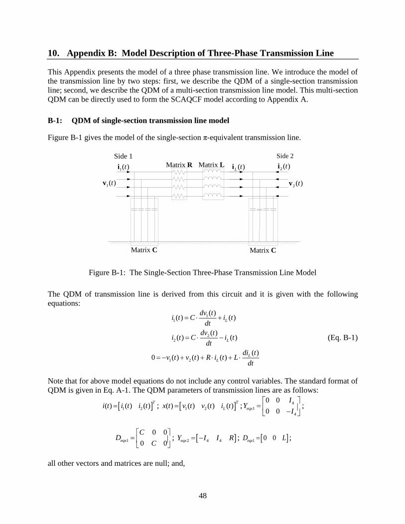
48
10. Appendix B: Model Description of Three-Phase Transmission Line
This Appendix presents the model of a three phase transmission line. We introduce the model of
the transmission line by two steps: first, we describe the QDM of a single-section transmission
line; second, we describe the QDM of a multi-section transmission line model. This multi-section
QDM can be directly used to form the SCAQCF model according to Appendix A.
B-1: QDM of single-section transmission line model
Figure B-1 gives the model of the single-section π-equivalent transmission line.
1( )ti
1( )tv2 ( )tv
Matrix R Matrix L
Matrix C Matrix C
( )L ti 2 ( )ti
Side 1 Side 2
Figure B-1: The Single-Section Three-Phase Transmission Line Model
The QDM of transmission line is derived from this circuit and it is given with the following
equations:
11
22
1 2
( ) ( ) ( )
( ) ( ) ( )
( )0 ( ) ( ) ( )
L
L
LL
dv ti t C i t
dt
dv ti t C i t
dt
di tv t v t R i t L
dt
(Eq. B-1)
Note that for above model equations do not include any control variables. The standard format of
QDM is given in Eq. A-1. The QDM parameters of transmission lines are as follows:
1 2( ) ( ) ( )T
i t i t i t ; 1 2( ) ( ) ( ) ( )T
Lx t v t v t i t ;4
1
4
0 0
0 0eqx
IY
I
;
1
0 0
0 0eqx
CD
C
; 2 4 4eqxY I I R ; 1 0 0eqxD L ;
all other vectors and matrices are null; and,

49
R , L and C are the resistance, inductance and capacitance matrices of the transmission line;
1( )i t and 2 ( )i t are current vectors at each side;
1( )v t and 2 ( )v t are voltage vectors at each side;
( )Li t is the current vector of the inductance.
4I is the identity matrix with dimension 4.
B-2: QDM of multi-section transmission line model
A multi-section π-equivalent model of the transmission line is used. The single section π-
equivalent model is accurate only for short lines. For a long transmission line, we divide the
transmission line into a proper number of sections where each section has the proper length to
ensure accuracy. The number of sections is chosen in such a way that the length of each section
should have a comparable travel time of electromagnetic waves to one sampling period. Next, the
combination procedure of single-section π-equivalent models is introduced as follows (section
number: n).
...
...
...1ai 1Li
1v
2ai 2Li1bi 3ai 3Li2bi 3bi 1nai 1nLi 1nbi nai nLi nbi
2v 3v nv 1nv
...
Figure B-2: Multi-section transmission line model
For section i :
( )aki t and ( )bki t represent 3-phase & neutral current at both sides of section k ;
( )kv t and 1( )kv t represent 3-phase & neutral voltage at both sides of section k ;
( )Lki t represents three-phase & neutral current through the inductance in section k ;
The equations that describe the above multi-section line are:
11 1 1 1 1
11 1 1
( )( ) ( ) ( )
( )( ) ( ) ( )
a L
nbn n Ln
dv ti t G v t i t C
dt
dv ti t G v t i t C
dt
(Eq. B-2)
Zero sum of currents between section k and section k+1 (k=1, 2, …, n-1):
1( 1) 1 1 1 ( 1)
( )0 ( ) ( ) 0 2 ( ) 2 ( )k
bk a k k Lk L k
dv ti t i t G v t C i t i
dt
(Eq. B-3)
Zero sum of voltage inside section k (k=1, 2, …, n):
1 1 1
( )0 ( ) ( ) ( ) Lk
k k Lk
di tv t v t R i t L
dt (Eq. B-4)
Similarly, the QDM parameters of the transmission line is as follows:

50
1( ) ( ) ( )T
a bni t i t i t ; 1 1 2 3 1 2( ) ( ) ( ) ( ) ( ) ( ) ( ) ( ) ( )T
n n L L Lnx t v t v t v t v t v t i t i t i t ;
1 4
1
1 4
0 0 0 0 0 0
0 0 0 0 0 0eqx
G IY
G I
;
1
1
1
0 0 0 0 0 0 0
0 0 0 0 0 0 0eqxd
CD
C
;
1 4 4
1 4
1 4
2
4 4 1
4 4 1
4 4 1
0 0 2 0 0 0
0 0 0 2 0 0 0
0 0 0 0 2 0 0
0 0 0 0 0
0 0 0 0 0
0 0 0 0 0
eqx
G I I
G I
G IY
I I R
I I R
I I R
;
1
1
1
2
1
1
1
0 0 2 0 0 0 0 0
0 0 0 2 0 0 0 0
0 0 0 0 2 0 0 0
0 0 0 0 0 0 0
0 0 0 0 0 0 0
0 0 0 0 0 0 0
eqxd
C
C
CD
L
L
L
;

51
11. Appendix C: Model Description of Three-Phase Two-Level PWM
Inverter
This Appendix presents the model of three-phase two-level PWM inverter. We introduce the
model of the inverter by three steps: first, we describe the overall model of the inverter; second,
we describe the single valve model; third, we describe the DC-side capacitor.
C-1: verall Model Description
In this section, we present the overall model of the three-phase two-level PWM inverter. As shown
in Figure C-1, the inverter model consists of a DC-side capacitor and detail models of six-valves.
AD
KD
A
B
CCDC
SWA_H
CSB
GSB
GSGD
CPGP
LCL GCL
SWA_L
SWB_H SWC_H
SWC_LCSB
GSB
GSGD
CPGP
LCL GCL
CSB
GSB
GSGD
CPGP
LCL GCL
CSB
GSB
GSGD
CPGP
LCL GCL
CSB
GSB
GSGD
CPGP
LCL GCL
SWB_L
CSB
GSB
GSGD
CPGP
LCL GCL
SWA_H_Valve
SWA_L_Valve
SWB_H_Valve
SWB_L_Valve
SWC_H_Valve
SWC_L_Valve
Figure C-1: Three-Phase Two-Level PWM Inverter Model
There is a complementary valve pair in each phase. For example, the complementary valve pair is
SWA_H_Valve and SWA_L_Valve for phase A. Thus in this Appendix, we only show switching
signals corresponding to the three-upper valves.
Each valve model consists of IGBT parasitic conductance, IGBT parasitic capacitance, IGBT-
on/off conductance, a snubber circuit, an anti-parallel diode, and a current-limiting circuit as
shown in Figure C-2.

52
ti
tV
tV
tV
tV
LCL
CP
CSB
2
1
States:
US(t)
Input:
tUS
If (US(t) == 1), GS = GSON
If (US(t) == 0), GS = GSOFF
If (VCP(t) 0), GD = GDOFF
If ( VCP(t) < 0), GD = GDON
IGBT-Conductance Determination
Anti-Parallel-Diode-Conductance Determination
V1(t), i1(t)
CSB
GSB
GSGD
CP
GP
LCL GCL
V2(t), i2(t)
iLCL(t)
+
VCP(t)
-+
VCSB(t)
-
Figure C-2: The Single Valve Model
As shown in the above figure, the IGBT switch has two conduction states determined by a
switching-signal input. Also, the anti-parallel diode also has two conduction states determined by
the polarity of the voltage across the parasitic capacitance. The conduction state of the IGBT switch
and anti-parallel diode are determined as follows:
2
1
1 1 12 2 2
S SON S SOFF S
DOFF DON DOFF DOND CP CP CP
G t G U t G U t
G G G GG t sign V t sign V t sign V t
(Eq. C-1)
where
1 0
0 0
1 0
if x
sign x if x
if x
Therefore, each valve model has four switching states as follows:
Valve State 0: IGBT Switch: ON and Diode: OFF (GS = GSON and GD = GDOFF),
Valve State 1: IGBT Switch: ON and Diode: ON (GS = GSON and GD = GDON),
Valve State 2: IGBT Switch: OFF and Diode: OFF (GS = GSOFF and GD = GDOFF),
Valve State 3: IGBT Switch: OFF and Diode: ON (GS = GSOFF and GD = GDON).

53
Each valve model determines its state and control algebraic quadratic companion form (SCAQCF) of
its current-time-step valve state from the predefined SCAQCFs of a single valve. By merging the
SCAQCFs of six-valve and DC-side capacitor models using Kirchhoff’s current law (KCL) at assigned
node numbers of the inverter model as shown in Figure C-3, we generate the SCAQCF of the inverter
model every time step. Figure C-4 shows the flow chart of the procedure. The above assigned node
numbers are stored in the following arrays as summarized in Table C-1.
AD
KD
A
B
CCDC
SWA_H
CSB
GSB
GSGD
CPGP
LCL GCL
SWA_L
SWB_H SWC_H
SWC_L
CSB
GSB
GSGD
CPGP
LCL GCL
CSB
GSB
GSGD
CPGP
LCL GCL
CSB
GSB
GSGD
CPGP
LCL GCL
CSB
GSB
GSGD
CPGP
LCL GCL
SWB_L
CSB
GSB
GSGD
CPGP
LCL GCL
0(28)
1(29)
2(30)
3(31)
4(32)
8(36)9(37)
10(38)
11(39) 12(40)
13(41)
14(42)15(43)
16(44)
17(45)18(46)
19(47)
20(48)21(49)
22(50)
23(51)24(52)
25(53)
Nodes at time t
Nodes at time tm
Switching-Signal Input Nodes:
5(33)
6(34)
7(35)
26(54)
27(55)
Figure C-3: Three-Phase Two-Level PWM Inverter Model with Assigned Node Numbers

54
Start
Switching-Signals Inputs
DetermineValve States ofSix-Valve Models
Four SCAQCFs of a Single Valve Model
for Four Valve States
Determineeach SCAQCF of
the Six-Valve Models
SCAQCFs ofa DC-Side Cpacitor Model
Merging the SCAQCFs ofthe Six-Valve and
the DC-Side CapacitorModels by KCL
SCAQCF Ofa Converter Model
Total Simulation Time
Elapsed?
End
Yes
No
Polarity of ParasiticCapacitorVoltages
Each SCAQCF Ofthe Six-Valve Models
Figure C-4: Procedure of the Generation of the SCAQCF of the Inverter Model

55
Table C-1: Assigned Node Numbers of the Three-Phase Two-Level PWM Inverter
t tm
External Internal External Internal
SWA_H 0 2 8 9 10 28 30 36 37 38
SWA_L 2 1 11 12 13 30 29 39 40 41
SWB_H 0 3 14 15 16 28 31 42 43 44
SWB_L 3 1 17 18 19 31 29 45 46 47
SWC_H 0 4 20 21 22 28 32 48 49 50
SWC_L 4 1 23 24 25 32 29 51 52 53
t tm
External Internal External Internal
DC-Side
Capacitor 0 1 26 27 28 29 54 55
C-2: Single Valve Model
The single valve model is provided in Figure C-2. The single valve model has four switching states.
The compact models for the four valve states are:
A. Valve State 0: Switch: ON and Diode: OFF (GS = GSON and GD = GDOFF):
𝑖1(t ) = 𝑖𝐿𝐶𝐿(𝑡) + 𝐺𝐶𝐿(𝑉1(𝑡) − 𝑉𝐶𝑃(𝑡) − 𝑉2(𝑡)) (Eq. C-2)
𝑖2(t ) = −𝑖𝐿𝐶𝐿(𝑡) − 𝐺𝐶𝐿(𝑉1(𝑡) − 𝑉𝐶𝑃(𝑡) − 𝑉2(𝑡)) (Eq. C-3)
0 = −𝑉𝐶𝑃(𝑡) +𝐶𝑆𝐵
𝐺𝑆𝐵∙
𝑑𝑉𝐶𝑆𝐵(𝑡)
𝑑𝑡+ 𝑉𝐶𝑆𝐵(𝑡) (Eq. C-4)
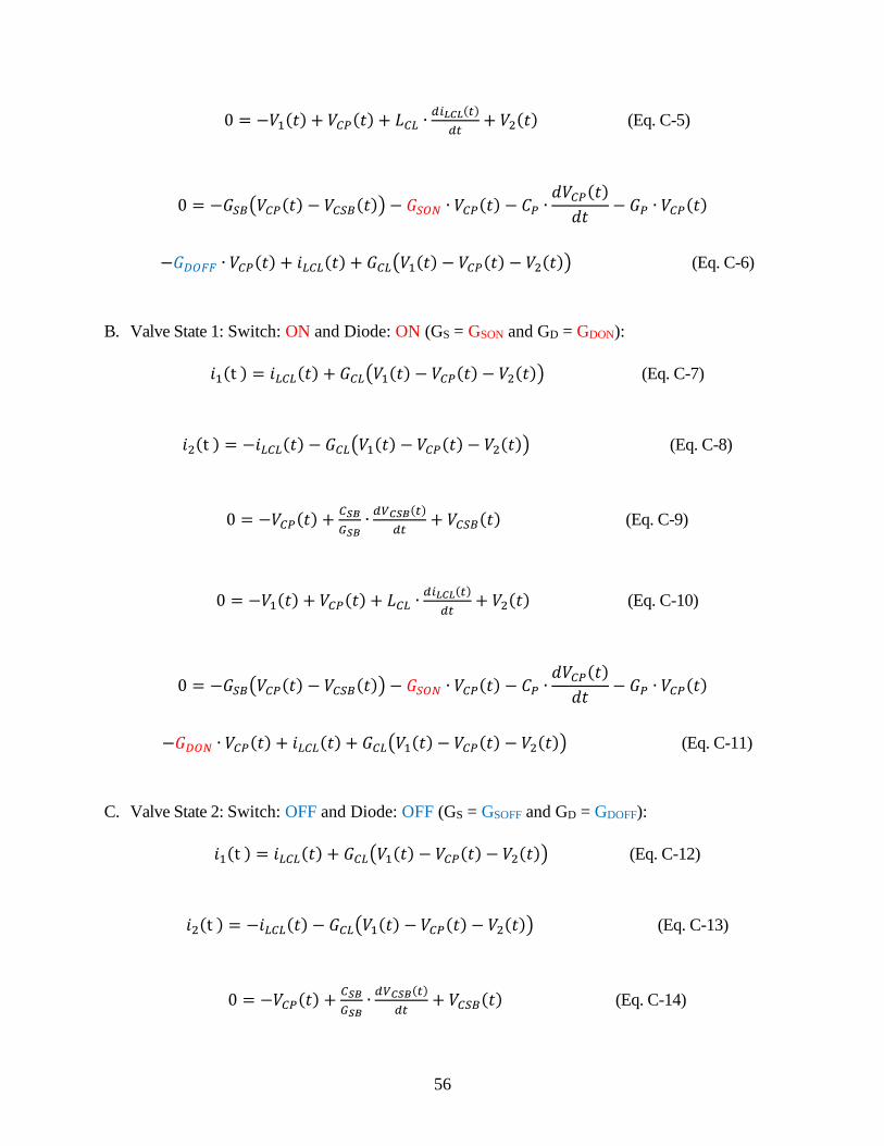
56
0 = −𝑉1(𝑡) + 𝑉𝐶𝑃(𝑡) + 𝐿𝐶𝐿 ∙𝑑𝑖𝐿𝐶𝐿(𝑡)
𝑑𝑡+ 𝑉2(𝑡) (Eq. C-5)
0 = −𝐺𝑆𝐵(𝑉𝐶𝑃(𝑡) − 𝑉𝐶𝑆𝐵(𝑡)) − 𝐺𝑆𝑂𝑁 ∙ 𝑉𝐶𝑃(𝑡) − 𝐶𝑃 ∙𝑑𝑉𝐶𝑃(𝑡)
𝑑𝑡− 𝐺𝑃 ∙ 𝑉𝐶𝑃(𝑡)
−𝐺𝐷𝑂𝐹𝐹 ∙ 𝑉𝐶𝑃(𝑡) + 𝑖𝐿𝐶𝐿(𝑡) + 𝐺𝐶𝐿(𝑉1(𝑡) − 𝑉𝐶𝑃(𝑡) − 𝑉2(𝑡)) (Eq. C-6)
B. Valve State 1: Switch: ON and Diode: ON (GS = GSON and GD = GDON):
𝑖1(t ) = 𝑖𝐿𝐶𝐿(𝑡) + 𝐺𝐶𝐿(𝑉1(𝑡) − 𝑉𝐶𝑃(𝑡) − 𝑉2(𝑡)) (Eq. C-7)
𝑖2(t ) = −𝑖𝐿𝐶𝐿(𝑡) − 𝐺𝐶𝐿(𝑉1(𝑡) − 𝑉𝐶𝑃(𝑡) − 𝑉2(𝑡)) (Eq. C-8)
0 = −𝑉𝐶𝑃(𝑡) +𝐶𝑆𝐵
𝐺𝑆𝐵∙
𝑑𝑉𝐶𝑆𝐵(𝑡)
𝑑𝑡+ 𝑉𝐶𝑆𝐵(𝑡) (Eq. C-9)
0 = −𝑉1(𝑡) + 𝑉𝐶𝑃(𝑡) + 𝐿𝐶𝐿 ∙𝑑𝑖𝐿𝐶𝐿(𝑡)
𝑑𝑡+ 𝑉2(𝑡) (Eq. C-10)
0 = −𝐺𝑆𝐵(𝑉𝐶𝑃(𝑡) − 𝑉𝐶𝑆𝐵(𝑡)) − 𝐺𝑆𝑂𝑁 ∙ 𝑉𝐶𝑃(𝑡) − 𝐶𝑃 ∙𝑑𝑉𝐶𝑃(𝑡)
𝑑𝑡− 𝐺𝑃 ∙ 𝑉𝐶𝑃(𝑡)
−𝐺𝐷𝑂𝑁 ∙ 𝑉𝐶𝑃(𝑡) + 𝑖𝐿𝐶𝐿(𝑡) + 𝐺𝐶𝐿(𝑉1(𝑡) − 𝑉𝐶𝑃(𝑡) − 𝑉2(𝑡)) (Eq. C-11)
C. Valve State 2: Switch: OFF and Diode: OFF (GS = GSOFF and GD = GDOFF):
𝑖1(t ) = 𝑖𝐿𝐶𝐿(𝑡) + 𝐺𝐶𝐿(𝑉1(𝑡) − 𝑉𝐶𝑃(𝑡) − 𝑉2(𝑡)) (Eq. C-12)
𝑖2(t ) = −𝑖𝐿𝐶𝐿(𝑡) − 𝐺𝐶𝐿(𝑉1(𝑡) − 𝑉𝐶𝑃(𝑡) − 𝑉2(𝑡)) (Eq. C-13)
0 = −𝑉𝐶𝑃(𝑡) +𝐶𝑆𝐵
𝐺𝑆𝐵∙
𝑑𝑉𝐶𝑆𝐵(𝑡)
𝑑𝑡+ 𝑉𝐶𝑆𝐵(𝑡) (Eq. C-14)
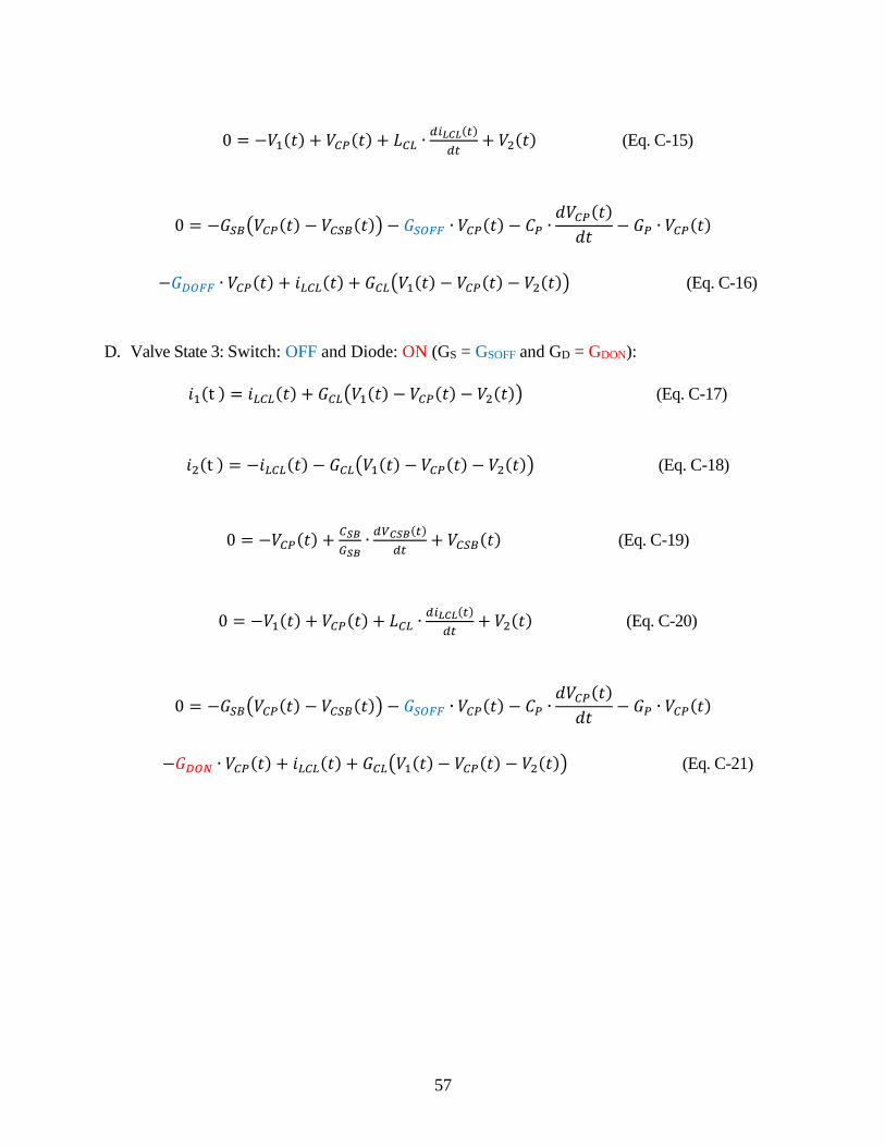
57
0 = −𝑉1(𝑡) + 𝑉𝐶𝑃(𝑡) + 𝐿𝐶𝐿 ∙𝑑𝑖𝐿𝐶𝐿(𝑡)
𝑑𝑡+ 𝑉2(𝑡) (Eq. C-15)
0 = −𝐺𝑆𝐵(𝑉𝐶𝑃(𝑡) − 𝑉𝐶𝑆𝐵(𝑡)) − 𝐺𝑆𝑂𝐹𝐹 ∙ 𝑉𝐶𝑃(𝑡) − 𝐶𝑃 ∙𝑑𝑉𝐶𝑃(𝑡)
𝑑𝑡− 𝐺𝑃 ∙ 𝑉𝐶𝑃(𝑡)
−𝐺𝐷𝑂𝐹𝐹 ∙ 𝑉𝐶𝑃(𝑡) + 𝑖𝐿𝐶𝐿(𝑡) + 𝐺𝐶𝐿(𝑉1(𝑡) − 𝑉𝐶𝑃(𝑡) − 𝑉2(𝑡)) (Eq. C-16)
D. Valve State 3: Switch: OFF and Diode: ON (GS = GSOFF and GD = GDON):
𝑖1(t ) = 𝑖𝐿𝐶𝐿(𝑡) + 𝐺𝐶𝐿(𝑉1(𝑡) − 𝑉𝐶𝑃(𝑡) − 𝑉2(𝑡)) (Eq. C-17)
𝑖2(t ) = −𝑖𝐿𝐶𝐿(𝑡) − 𝐺𝐶𝐿(𝑉1(𝑡) − 𝑉𝐶𝑃(𝑡) − 𝑉2(𝑡)) (Eq. C-18)
0 = −𝑉𝐶𝑃(𝑡) +𝐶𝑆𝐵
𝐺𝑆𝐵∙
𝑑𝑉𝐶𝑆𝐵(𝑡)
𝑑𝑡+ 𝑉𝐶𝑆𝐵(𝑡) (Eq. C-19)
0 = −𝑉1(𝑡) + 𝑉𝐶𝑃(𝑡) + 𝐿𝐶𝐿 ∙𝑑𝑖𝐿𝐶𝐿(𝑡)
𝑑𝑡+ 𝑉2(𝑡) (Eq. C-20)
0 = −𝐺𝑆𝐵(𝑉𝐶𝑃(𝑡) − 𝑉𝐶𝑆𝐵(𝑡)) − 𝐺𝑆𝑂𝐹𝐹 ∙ 𝑉𝐶𝑃(𝑡) − 𝐶𝑃 ∙𝑑𝑉𝐶𝑃(𝑡)
𝑑𝑡− 𝐺𝑃 ∙ 𝑉𝐶𝑃(𝑡)
−𝐺𝐷𝑂𝑁 ∙ 𝑉𝐶𝑃(𝑡) + 𝑖𝐿𝐶𝐿(𝑡) + 𝐺𝐶𝐿(𝑉1(𝑡) − 𝑉𝐶𝑃(𝑡) − 𝑉2(𝑡)) (Eq. C-21)

58
From Appendix A, the SCAQCF of a single valve is (all other matrices are null):
A. Valve State 0:
0 0
eqx
0 1 0 0 0 0 0
0 1 0 0 0 0 0
2 20 0 0 0 0 0
6 6 3 3
2 2 20 0 0
6 6 6 3 3 3
2 2 2 2 2
6 6 6 6 6 3 3 3 3 3Y
0 0 0 0 0 0 1
0 0 0 0 0 0 1
0 0 0 0 024 24 3
CL CL CL
CL CL CL
SB
SB
CL
CL CL SB P CL CL SB
CL CL CL
CL CL CL
SB
SB
G G G
G G G
C h h h h
G
h h h h h hL
h h h h h h h h h hG G G K C G G G K
G G G
G G G
Ch h h
G
0 0
03
0 0 024 24 24 3 3 3
24 24 24 24 24 3 3 3 3 3
CL
CL CL SB CL CL SB P
h
h h h h h hL
h h h h h h h h h hG G G K G G G K C
0
eqx
0
0 1
0 1
0 0 06 6
06 6 6
6 6 6 6 6
1 1 1 1N 02 2 2 2
1 1 1 10
2 2 2 2
5 50 0 0
24 24
5 5 50
24 24 24
5 5 5 5 5
24 24 24 24 24
CL CL CL
CL CL CL
SB
SB
CL
CL CL SB P
CL CL CL
CL CL CL
SB
SB
CL
CL CL SB P
G G G
G G G
C h h
G
h h hL
h h h h hG G G K C
G G G
G G G
C h h
G
h h hL
h h h h hG G G K C
,
00
00
002
10
02
100
00
00
10
01
M eq

59
Where 𝐾0 = 𝐺𝑆𝐵 + 𝐺𝑆𝑂𝑁 + 𝐺𝑃 + 𝐺𝐷𝑂𝐹𝐹 + 𝐺𝐶𝐿;
B. Valve State 1:
1 1
eqx
0 1 0 0 0 0 0
0 1 0 0 0 0 0
2 20 0 0 0 0 0
6 6 3 3
2 2 20 0 0
6 6 6 3 3 3
2 2 2 2 2
6 6 6 6 6 3 3 3 3 3Y
0 0 0 0 0 0 1
0 0 0 0 0 0 1
0 0 0 0 024 24 3
CL CL CL
CL CL CL
SB
SB
CL
CL CL SB P CL CL SB
CL CL CL
CL CL CL
SB
SB
G G G
G G G
C h h h h
G
h h h h h hL
h h h h h h h h h hG G G K C G G G K
G G G
G G G
Ch h h
G
1 1
03
0 0 024 24 24 3 3 3
24 24 24 24 24 3 3 3 3 3
CL
CL CL SB CL CL SB P
h
h h h h h hL
h h h h h h h h h hG G G K G G G K C
1
eqx
1
0 1
0 1
0 0 06 6
06 6 6
6 6 6 6 6
1 1 1 1N 02 2 2 2
1 1 1 10
2 2 2 2
5 50 0 0
24 24
5 5 50
24 24 24
5 5 5 5 5
24 24 24 24 24
CL CL CL
CL CL CL
SB
SB
CL
CL CL SB P
CL CL CL
CL CL CL
SB
SB
CL
CL CL SB P
G G G
G G G
C h h
G
h h hL
h h h h hG G G K C
G G G
G G G
C h h
G
h h hL
h h h h hG G G K C
00
00
002
10
02
100
00
00
10
01
M eq
where 𝐾1 = 𝐺𝑆𝐵 + 𝐺𝑆𝑂𝑁 + 𝐺𝑃 + 𝐺𝐷𝑂𝑁 + 𝐺𝐶𝐿;

60
C. Valve State 2:
2 2
eqx
0 1 0 0 0 0 0
0 1 0 0 0 0 0
2 20 0 0 0 0 0
6 6 3 3
2 2 20 0 0
6 6 6 3 3 3
2 2 2 2 2
6 6 6 6 6 3 3 3 3 3Y
0 0 0 0 0 0 1
0 0 0 0 0 0 1
0 0 0 0 024 24 3
CL CL CL
CL CL CL
SB
SB
CL
CL CL SB P CL CL SB
CL CL CL
CL CL CL
SB
SB
G G G
G G G
C h h h h
G
h h h h h hL
h h h h h h h h h hG G G K C G G G K
G G G
G G G
Ch h h
G
2 2
03
0 0 024 24 24 3 3 3
24 24 24 24 24 3 3 3 3 3
CL
CL CL SB CL CL SB P
h
h h h h h hL
h h h h h h h h h hG G G K G G G K C
,
2
eqx
2
0 1
0 1
0 0 06 6
06 6 6
6 6 6 6 6
1 1 1 1N 02 2 2 2
1 1 1 10
2 2 2 2
5 50 0 0
24 24
5 5 50
24 24 24
5 5 5 5 5
24 24 24 24 24
CL CL CL
CL CL CL
SB
SB
CL
CL CL SB P
CL CL CL
CL CL CL
SB
SB
CL
CL CL SB P
G G G
G G G
C h h
G
h h hL
h h h h hG G G K C
G G G
G G G
C h h
G
h h hL
h h h h hG G G K C
,
00
00
002
10
02
100
00
00
10
01
M eq
where 𝐾2 = 𝐺𝑆𝐵 + 𝐺𝑆𝑂𝐹𝐹 + 𝐺𝑃 + 𝐺𝐷𝑂𝐹𝐹 + 𝐺𝐶𝐿 ;

61
D. Valve State 3:
3 3
eqx
0 1 0 0 0 0 0
0 1 0 0 0 0 0
2 20 0 0 0 0 0
6 6 3 3
2 2 20 0 0
6 6 6 3 3 3
2 2 2 2 2
6 6 6 6 6 3 3 3 3 3Y
0 0 0 0 0 0 1
0 0 0 0 0 0 1
0 0 0 0 024 24 3
CL CL CL
CL CL CL
SB
SB
CL
CL CL SB P CL CL SB
CL CL CL
CL CL CL
SB
SB
G G G
G G G
C h h h h
G
h h h h h hL
h h h h h h h h h hG G G K C G G G K
G G G
G G G
Ch h h
G
3 3
03
0 0 024 24 24 3 3 3
24 24 24 24 24 3 3 3 3 3
CL
CL CL SB CL CL SB P
h
h h h h h hL
h h h h h h h h h hG G G K G G G K C
3
eqx
3
0 1
0 1
0 0 06 6
06 6 6
6 6 6 6 6
1 1 1 1N 02 2 2 2
1 1 1 10
2 2 2 2
5 50 0 0
24 24
5 5 50
24 24 24
5 5 5 5 5
24 24 24 24 24
CL CL CL
CL CL CL
SB
SB
CL
CL CL SB P
CL CL CL
CL CL CL
SB
SB
CL
CL CL SB P
G G G
G G G
C h h
G
h h hL
h h h h hG G G K C
G G G
G G G
C h h
G
h h hL
h h h h hG G G K C
,
00
00
002
10
02
100
00
00
10
01
M eq
where 𝐾3 = 𝐺𝑆𝐵 + 𝐺𝑆𝑂𝐹𝐹 + 𝐺𝑃 + 𝐺𝐷𝑂𝑁 + 𝐺𝐶𝐿 ;

62
C-3: DC-side capacitor model
This section presents the DC-side capacitor model.
+
VC(t)
-
y(t)
V1(t), i1(t)
V2(t), i2(t)
CDC
Figure C-5: DC-Side Capacitor Model
The single valve model is provided in Figure C-5. The DC-side capacitor model is:
𝑖1(𝑡) = 𝐶𝐷𝐶 ∙ 𝑦1(𝑡) (Eq. C-22)
𝑖2(𝑡) = −𝐶𝐷𝐶 ∙ 𝑦1(𝑡) (Eq. C-23)
0 =𝑑𝑉𝐶(𝑡)
𝑑𝑡− 𝑦1(𝑡) (Eq. C-24)
0 = 𝑉𝐶(𝑡) − 𝑉1(𝑡) + 𝑉2(𝑡) (Eq. C-25)
From Appendix A, the SCAQCF of the DC-side capacitor is (all other matrices are null):
x
0 0 0 0 0 0 0
0 0 0 0 0 0 0
20 0 1 0 0 0
6 3
1 1 1 0 0 0 0 0
0 0 0 0 0 0 0
0 0 0 0 0 0 0
0 0 0 0 0 124 3
0 0 0 0 1 1 1 0
DC
DC
eq
DC
DC
C
C
h h
YC
C
h h

63
x
0 0 0
0 0 0
0 0 16
0 0 0 0
0 0 02
0 0 02
50 0 1
24
0 0 0 0
DC
DC
DCeq
DC
C
C
h
CN
C
h
00
002
10
02
100
00
10
01
eqM

64
12. Appendix D: Model Description of the Digital Signal Processor (DSP)
This Appendix presents the digital signal processor (DSP). The DSP digitally filters raw analog
signals into digital signals of fundamental frequency. The DSP outputs are: the positive sequence
phasor of three-phase voltages (��1) and currents (𝐼1), the fundamental frequency, three-phase real
(P) and reactive power (Q), the actual average fundamental frequency (fs), the next zero-crossing
time from the negative to positive of the voltage positive-sequence waveform (ZX), the rate of
average frequency change (𝑑𝑓𝑠
𝑑𝑡), and DC-link average voltage ( ��𝐷𝐶 ). The DSP receives
instantaneous value inputs Van, Vbn, Vcn, Ia, Ib, Ic , and VDC then calculates outputs, ��1, 𝐼1, P, Q, fs,
ZX, 𝑑𝑓𝑠
𝑑𝑡, and ��𝐷𝐶 as shown in Figure D-1.
Digital Signal Processor
anV
bnV
cnV
aI
bI
cI
1
~V
1
~I
P
Q
sf
ZX
dt
df s
DCVDCV
Figure D-1: Block Diagram of the Digital Signal Processor
This Appendix is arranged as follows. Section D-1 describes the calculation of frequency and the
rate of frequency change; section D-2 and D-3 describes the calculation process of positive
sequence voltage and current phasors; section D-4 describes the calculation of three-phase
fundamental frequency real and reactive power; section D-5 describes the calculation of next zero-
crossing time.
D-1: Frequency and the Rate of Frequency Change
To calculate the actual average fundamental frequency and rate of average frequency change, we
are using a method based on the calculation of the rate of phase angle changes of input data, Van,
Vbn, Vcn, Ia, Ib, and Ic. A computationally efficient recursive implementation is described as follows.
The following two sums are recursively updated every time when a new input data sample, x(i),
becomes available:

65
1
1_
1cos
k N
x s r
i k
V k x i T iN
(Eq D-1)
1
2 _
1sin
k N
x s r
i k
V k x i T iN
(Eq. D-2)
2s sf (Eq. D-3)
where:
ix : Input data samples.
fs: Actual average fundamental frequency. It is initialized as the nominal power
frequency, 60 Hz, for the first iteration, but it is updated every recursive loop of the
calculation of the average frequency.
rT : Sampling period of the analog-to-digital converter.
N: Number of samples in a period
rsT
2.
At every sample the two sums are updated, and the phase angle, , is computed as follows:
kV
kVk
x
x
x
_1
_21tan . (Eq. D-4)
The actual fundamental frequency of ix is computed from the rate of change of the above value
as follows:
r
kx
sxsT
kfkf
21
_
_
. (Eq. D-5)
where 1_ kk xxkx .
By applying the above actual fundamental frequency calculation method to the input data, Van, Vbn,
Vcn, Ia, Ib, and Ic, we can calculate the actual fundamental frequencies of the input data as follows:
a) kfanVs _ :
1
_1 cos1 Nk
ki
rsanV iTiVN
kVan
(Eq. D-6)
1
_2 sin1 Nk
ki
rsanV iTiVN
kVan
(Eq. D-7)

66
kV
kVk
an
an
an
V
V
V
_1
_21tan (Eq. D-8)
1_ kkananan VVkV (Eq. D-9)
r
V
sVsT
kff kan
an
21 _
_
(Eq D-10)
b) kfbnVs _
1
_1 cos1 Nk
ki
rsbnV iTiVN
kVbn
(Eq. D-11)
1
_2 sin1 Nk
ki
rsbnV iTiVN
kVbn
(Eq. D-12)
kV
kVk
bn
bn
bn
V
V
V
_1
_21tan (Eq. D-13)
1_ kkbnbnbn VVkV (Eq. D-14)
r
V
sVsT
kffkbn
bn
21
_
_
(Eq. D-15)
c) kfcnVs _
1
_1 cos1 Nk
ki
rscnV iTiVN
kVcn
(Eq. D-16)
1
_2 sin1 Nk
ki
rscnV iTiVN
kVcn
(Eq.D-17)

67
kV
kVk
cn
cn
cn
V
V
V
_1
_21tan (Eq. D-18)
1_ kkcncncn VVkV (Eq. D-19)
r
V
sVsT
kffkcn
cn
21
_
_
(Eq. D-20)
d) kfaIs _
1
_1 cos1 Nk
ki
rsaI iTiIN
kVa
(Eq. D-21)
1
_2 sin1 Nk
ki
rsaI iTiIN
kVa
(Eq. D-22)
kV
kVk
a
a
a
I
I
I
_1
_21tan (Eq. D-23)
1_ kkaaa IIkI (Eq. D-24)
r
I
sIsT
kff ka
a
21 _
_
(Eq. D-25)
e) kfbIs _
1
_1 cos1 Nk
ki
rsbI iTiIN
kVb
(Eq. D-26)
1
_2 sin1 Nk
ki
rsbI iTiIN
kVb
(Eq. D-27)

68
kV
kVk
b
b
b
I
I
I
_1
_21tan (Eq. D-28)
1_ kkbbb IIkI (Eq. D-29)
r
I
sIsT
kff kb
b
21 _
_
(Eq. D-30)
f) kfcIs _
1
_1 cos1 Nk
ki
rscI iTiIN
kVc
(Eq. D-31)
1
_2 sin1 Nk
ki
rscI iTiIN
kVc
(Eq. D-32)
kV
kVk
b
b
b
I
I
I
_1
_21tan (Eq. D-33)
1_ kkccc IIkI (Eq. D-34)
r
I
sIsT
kffkc
c
21
_
_
(Eq. D-35)
Finally, we can calculate the average fundamental frequency, fs, and rate of average frequency
change as follows:
6
______ kfkfkfkfkfkfkf cbacnbnan IsIsIsVsVsVs
s
(Eq. D-36)
r
sss
T
kfkf
dt
kdf 1 (Eq. D-37)

69
D-2: Positive Sequence Voltage Phasor
In this section, we present the calculation of positive sequence voltage phasor 1V using three-phase
voltages updated every recursive loop in the previous section. First, we calculate the fundamental
voltage phasors anV , bnV , and cnV as follows:
2_2
2
_1 kVkVkVanan VVan (Eq. D-38)
2_2
2
_1 kVkVkVbnbn VVbn (Eq. D-39)
2_2
2
_1 kVkVkVcncn VVcn (Eq. D-40)
kkV
kVanV
an
an 2
~ (Eq. D-41)
kkV
kVbnV
bn
bn 2
~ (Eq. D-42)
kkV
kVcnV
cn
cn 2
~ (Eq. D-43)
In the next step, we are calculating the positive sequence voltage phasor from the obtained
fundamental frequency voltage phasors by using the symmetrical component transformation based
modal decomposition. The symmetrical component transformation is expressed as follows:
2
1
2
2
0
11
13
1 1 1
an
bn
cn
V k a a V k
V k a a V k
V k V k
, where 3
2j
ea (Eq. D-44)
where ��1, ��2, and ��0 are the positive, negative and zero sequence voltage phasors, respectively.
By using this, we can calculate the positive-sequence voltage phasor ��1, of three-phase voltages
Van, Vbn, and Vcn, as follows:
2 4
3 31
1 1
3 3
j j
an bn cnV k V k V k e V k e V k jV k
. (Eq. D-45)

70
where
3
4cos
23
2cos
2cos
2
k
kVk
kVk
kVkV
cnbnan V
cn
V
bn
V
an (Eq. D-46)
3
4sin
23
2sin
2sin
2
k
kVk
kVk
kVkV
cnbnan V
cn
V
bn
V
an (Eq. D-47)
1
1tanV
V kk
V k
(Eq. D-48)
2 2
1
1+
3V k V k V k . (Eq. D-49)
D-3: Positive-Sequence Current Phasor
In this section, we calculate the positive sequence current phasor using the same method presented
in the previous section. By using three-phase currents updated every recursive loop in section D-
1. We first calculate the fundamental frequency current phasors of aI , bI and cI as follows:
2_2
2
_1 kVkVkIaa IIa , (Eq. D-50)
2_2
2
_1 kVkVkIbb IIb , (Eq. D-51)
2_2
2
_1 kVkVkIcc IIc (Eq. D-52)
kkI
kIaI
a
a 2
~ (Eq. D-53)
kkI
kIbI
b
b 2
~ (Eq. D-54)
kkI
kIcI
c
c 2
~ (Eq. D-55)
Then, we compute the positive sequence current phasor 𝐼1 by using the symmetrical component
transformation as follows:

71
kI
kI
kI
aa
aa
kI
kI
kI
c
b
a
~
~
~
111
1
1
3
1
~
~
~
2
2
0
2
1
, where 3
2j
ea (Eq. D-56)
2 4
3 31
1 1
3 3
j j
a b cI k I k I k e I k e I k jI k
(Eq. D-57)
where
3
4cos
23
2cos
2cos
2
k
kIk
kIk
kIkI
cba I
c
I
b
I
a (Eq. D-58)
3
4sin
23
2sin
2sin
2
k
kIk
kIk
kIkI
cba I
c
I
b
I
a (Eq. D-59)
1
1tanI
I kk
I k
(Eq. D-60)
2 2
1
1+
3I k I k I k (Eq. D-61)
D-4: Fundamental Frequency Real and Reactive Power
In this section, we calculate the fundamental frequency three-phase real and reactive power from
the extracted fundamental frequency voltage and current phasors as follows:
* * *Re an a bn b cn cP k V k I k V k I k V k I k (Eq. D-62)
* * *Im an a bn b cn cQ k V k I k V k I k V k I k (Eq. D-63)
D-5: Next Zero-Crossing Time
With the obtained positive sequence voltage phasor ��1, we can calculate the next zero-crossing
time from negative to positive. By defining that the voltage in the time domain is the cosine
function, we can convert the positive sequence voltage phasor ��1 into the time-domain
representation 𝑉1(𝑡), as follows:
kkVkV V111
~~ (Eq. D-64)

72
ktkfkVtV Vs 12cos
~2 11 (Eq. D-65)
As shown in Figure. D-2, the zero crossing from negative to positive occurs in every 360°, or time 1
𝑓𝑠(𝑘) sec. Thus, we can calculate the next zero-crossing time from negative to positive, 𝑡𝑛1+1, as
follows:
212cos
~22cos
~2 111111 111
nkVktkfkVtV Vnsn (Eq. D-
66)
2
122 11 11
nktkf Vns (Eq. D-67)
kf
kn
kft
s
V
s
n
221
1 1
1 11 (Eq. D-68)
where 𝑛1 = 𝑖𝑛𝑡 (𝜔𝑠𝑡𝑅+𝜃𝑉1
(𝑘)
2𝜋) and tR is the present time.
cos
2
3
2
32
2
32
-
+
-
+-
+
Figure D-2: Cosine Function with respect to the Phase Angle

73
D-6: Average DC-Input Voltage
The average DC-input voltage is computed as follows:
11 Nk
ki
DCDC iVN
kV (Eq. D-71)
where:
𝑉𝐷𝐶(𝑖): Input data sample sequence of the DC-input voltage.
N: The number of samples in the 1
6 of a period (=
1
6∙
1
𝑓𝑠∙𝑇𝑟).
𝑇𝑟: Sampling period of the analog-to-digital converter.
𝑓𝑠: The actual average fundamental frequency.

74
13. Appendix E: Master Thesis by Christopher Weldy
This Appendix presents the summary of the Master Thesis by Christopher Weldy. The full Thesis
is available on the Georgia Tech archives.
SUMMARY
STABILITY OF A 24-BUS POWER SYSTEM WITH
CONVERTER INTERFACED GENERATION
The objective of this Masters Thesis is to investigate the system stability implications of
integration of power electronic converter interfaced generation (CIG) into conventional power
systems. Due to differences between conventional generation and CIG, the power system fault
currents, voltage response, and frequency response will likely change with increased penetration
of CIG. This research will use state of the art software tools to perform simulations on the IEEE
24-Bus Reliability Test System (RTS-24), appropriately modified to include converter interfaced
generation. Time-domain dynamic simulations and fault calculations will be performed for the
system. A comprehensive set of simulations will be performed on the base case, comprised entirely
of conventional generation. Conventional generation will be replaced by CIG in the model, one
generating station at a time until CIG penetration is one-hundred percent. The comprehensive set
of simulations will be performed at each level of CIG penetration. The results will be compared to
the base case, with a focus on voltage response, frequency response, and fault current levels of the
power system.
As conventional generation is replaced by CIG the system frequency declines to lower and lower
minimum values in response to disturbances. Furthermore, the system voltages oscillate at higher
and higher frequencies and resolve at undesirable deviations from their initial values. These
undesirable results, however, can be mitigated by active and reactive power injections in response
to system disturbances. To mitigate some of the issues observed in the maximum CIG power
system, active and reactive power injections were modeled to represent the potential contribution
to dynamic stability of the system. Use of active power injection in response to a fault can mitigate
some of the additional frequency dip caused by reduction in generator inertia. Use of reactive
power injection in response to a fault can mitigate some of the voltage deviation observed due to
insufficient reactive power margin of available generation.
Power electronic converter rating limits have a significant impact on fault current levels in the
system, but the network impedance can reduce the impact of these converter limitations at
locations remote from the converter. As penetration of CIG into power systems increases, fault
current levels may begin to approach load current levels. This condition may require new
protection methods to maintain reliable and secure protection as power systems evolve.

Part II
Development of Positive Sequence Converter Models
and Demonstration of Approach on the WECC System
Vijay Vittal
Rajapandian Ayyanar
Arizona State University
Graduate Students:
Deepak Ramasubramanian
Ziwei Yu
Arizona State University

For more information about Part II, contact:
Vijay Vittal
Director, Power Systems Engineering Research Center
Ira A. Fulton Chair Professor
Arizona State University
PO Box 875706
Tempe, AZ 85287-5706
Phone: (480) 965-1879
E-Mail: [email protected]
Phone: (480) 965-1879
Power Systems Engineering Research Center
The Power Systems Engineering Research Center (PSERC) is a multi-university Center
conducting research on challenges facing the electric power industry and educating the next
generation of power engineers. More information about PSERC can be found at the Center’s
website: http://www.pserc.org.
For additional information, contact:
Power Systems Engineering Research Center
Arizona State University
551 E. Tyler Mall
Engineering Research Center #527
Tempe, Arizona 85287-5706
Phone: (480) 965-1643
Fax: (480) 965-0745
Notice Concerning Copyright Material
PSERC members are given permission to copy without fee all or part of this publication for internal
use if appropriate attribution is given to this document as the source material. This report is
available for downloading from the PSERC website.
©2016 Arizona State University. All rights reserved.

TABLE OF CONTENTS
LIST OF FIGURES . . . . . . . . . . . . . . . . . . . . . . . . . . iii
LIST OF TABLES . . . . . . . . . . . . . . . . . . . . . . . . . . . vii
LIST OF SYMBOLS . . . . . . . . . . . . . . . . . . . . . . . . . . viii
1 INTRODUCTION . . . . . . . . . . . . . . . . . . . . . . . . . 1
1.1 Background . . . . . . . . . . . . . . . . . . . . . . . . . . . . . . . . . 1
1.2 Motivation and Objectives . . . . . . . . . . . . . . . . . . . . . . . . . 3
1.3 Organization of the Report . . . . . . . . . . . . . . . . . . . . . . . . .5
2 LITERATURE REVIEW. . . . . . . . . . . . . . . . . . . . . . . 6
3 MATHEMATICAL MODEL OF THE POWER SYSTEM . . . . . . . . . 11
3.1 Synchronous Generator Model . . . . . . . . . . . . . . . . . . . . . . .11
3.1.1 TheE ′′ Model . . . . . . . . . . . . . . . . . . . . . . . . . . . . 12
3.1.2 TheE ′ Model . . . . . . . . . . . . . . . . . . . . . . . . . . . . 13
3.1.3 Classical Model . . . . . . . . . . . . . . . . . . . . . . . . . . . 14
3.2 Governor Model . . . . . . . . . . . . . . . . . . . . . . . . . . . . . . . 15
3.3 Static Exciter Model . . . . . . . . . . . . . . . . . . . . . . . . . . . . . 16
3.4 Load Model . . . . . . . . . . . . . . . . . . . . . . . . . . . . . . . . . 17
3.5 Network Model . . . . . . . . . . . . . . . . . . . . . . . . . . . . . . . 18
4 MODELING OF CONVERTERS . . . . . . . . . . . . . . . . . . . 21
4.1 The Converter Model in Commercial Software (pv1g,gewtg) . . . . . . . 21
4.2 The Converter Control Model in Commercial Software (pv1e,ewtgfc) . . 23
4.3 User Defined Converter Control Model . . . . . . . . . . . . . . . . .. . 24
4.4 Induction Motor Drive Model . . . . . . . . . . . . . . . . . . . . . . . .30
5 SIMULATION AND RESULTS . . . . . . . . . . . . . . . . . . . . 32
5.1 Converter Model Validation in a Two Machine System . . . . .. . . . . 32
5.2 Results in Commercial Software . . . . . . . . . . . . . . . . . . . . .. 35
i

5.2.1 Small Scale System-Validation of Results . . . . . . . . . .. . . 36
5.2.2 Large Scale System-Economy of Computation . . . . . . . . .. 44
5.3 Note on Boundary Current Representation of Converter . .. . . . . . . . 51
5.4 All CIG WECC system . . . . . . . . . . . . . . . . . . . . . . . . . . . 52
5.4.1 Generation Outage (100% CIG penetration) . . . . . . . . . .. . 52
5.4.2 Dc Voltage Dip and Subsequent Recovery (100% CIG penetration) 57
5.4.3 Line Fault followed by Outage (100% CIG penetration) .. . . . . 59
5.4.4 Bus Fault (100% CIG penetration) . . . . . . . . . . . . . . . . . 59
5.4.5 Line Reconnection (100% CIG penetration) . . . . . . . . . .. . 62
5.5 Induction Motor Drive Model . . . . . . . . . . . . . . . . . . . . . . . .64
6 CONCLUSION AND FUTURE RESEARCH . . . . . . . . . . . . . . 68
REFERENCES . . . . . . . . . . . . . . . . . . . . . . . . . . . . 70
APPENDICES . . . . . . . . . . . . . . . . . . . . . . . . . . . . 75
A EPCL CODE FOR USER DEFINED CONVERTER CONTROL MODEL . . . 75
B THREE GENERATOR EQUIVALENT SYSTEM DATA . . . . . . . . . . 83
B.1 Power flow solution . . . . . . . . . . . . . . . . . . . . . . . . . . . . . 83
B.2 Dynamic data . . . . . . . . . . . . . . . . . . . . . . . . . . . . . . . . 83
ii

LIST OF FIGURES
Figure 1.1 Sources of electricity generation in U.S. in 2013[1] . . . . . . . . 1
Figure 3.1 E ′′ model equivalent circuit . . . . . . . . . . . . . . . . . . . . . 12
Figure 3.2 E ′ model equivalent circuit . . . . . . . . . . . . . . . . . . . . . 14
Figure 3.3 Droop characteristic . . . . . . . . . . . . . . . . . . . . . . .. . 15
Figure 3.4 Governor based on droop characteristics . . . . . . .. . . . . . . 16
Figure 3.5 Static exciter basic framework . . . . . . . . . . . . . . .. . . . . 17
Figure 3.6 Machine and network reference frames for machinei . . . . . . . 19
Figure 4.1 Modeling solar photovoltaic plants in PSLF [2] . . . . . . . . . . . 21
Figure 4.2 Modeling wind turbine-generators in PSLF [3] . . . . . . . . . . . 22
Figure 4.3 Converter model in PSLF [4] . . . . . . . . . . . . . . . . . . . . 23
Figure 4.4 Converter control model in PSLF [4] . . . . . . . . . . . . . . . . 24
Figure 4.5 User defined converter control model . . . . . . . . . . .. . . . . 25
Figure 4.6 Variation ofQlimit with Vt . . . . . . . . . . . . . . . . . . . . . . 26
Figure 4.7 Conversion from windup to anti-windup limit . . . .. . . . . . . 27
Figure 4.8 Inner current control loop in PLECS to generate PWM reference
voltage wave . . . . . . . . . . . . . . . . . . . . . . . . . . . . . . . . . 28
Figure 4.9 Boundary current converter representation for positive sequence
simulation . . . . . . . . . . . . . . . . . . . . . . . . . . . . . . . . . . 28
Figure 4.10 Voltage source converter representation for positive sequence sim-
ulation . . . . . . . . . . . . . . . . . . . . . . . . . . . . . . . . . . . . 29
Figure 4.11 Modified active power controller for voltage source converter rep-
resentation . . . . . . . . . . . . . . . . . . . . . . . . . . . . . . . . . . 29
Figure 4.12 Control diagram of induction motor speed control drive . . . . . . 31
Figure 5.1 Two machine system . . . . . . . . . . . . . . . . . . . . . . . . . 32
Figure 5.2 Comparison of the converter active power output between PLECS
and positive sequence simulation . . . . . . . . . . . . . . . . . . . . . .33
Figure 5.3 Phase voltage waveforms at the converter terminal from PLECS . . 34
Figure 5.4 Line current waveforms at the converter terminalfrom PLECS . . 34
Figure 5.5 Converter active power output for different PLL gains . . . . . . . 35
iii

Figure 5.6 Three machine nine bus equivalent system . . . . . . .. . . . . . 36
Figure 5.7 Comparison of the active power output of converter at bus 1 be-
tween PLECS and the ‘epcgen’ model in PSLF with synchronous ma-
chines at buses 2 and 3 . . . . . . . . . . . . . . . . . . . . . . . . . . . 37
Figure 5.8 Comparison of the reactive power output of converter at bus 1 be-
tween PLECS and the ‘epcgen’ model in PSLF with synchronous ma-
chines at buses 2 and 3 . . . . . . . . . . . . . . . . . . . . . . . . . . . 38
Figure 5.9 Comparison of the terminal voltage of converter at bus 1 between
PLECS and the ‘epcgen’ model in PSLF with synchronous machines at
buses 2 and 3 . . . . . . . . . . . . . . . . . . . . . . . . . . . . . . . . 39
Figure 5.10 Sensitivity of the terminal voltage of converter at bus 1 for positive
sequence voltage source representation to different values of filter inductor 40
Figure 5.11 Active power output of the converters for an all CIG system with
increase in active power load . . . . . . . . . . . . . . . . . . . . . . . . 41
Figure 5.12 Reactive power output of the converters for an all CIG system with
increase in active power load . . . . . . . . . . . . . . . . . . . . . . . . 42
Figure 5.13 Frequency response of an all CIG system with increase in reactive
power load . . . . . . . . . . . . . . . . . . . . . . . . . . . . . . . . . . 42
Figure 5.14 Voltage magnitudes of an all CIG system with increase in reactive
power load . . . . . . . . . . . . . . . . . . . . . . . . . . . . . . . . . . 43
Figure 5.15 Active power output of the converters for an all CIG system with
increase in reactive power load . . . . . . . . . . . . . . . . . . . . . . . 43
Figure 5.16 Reactive power output of the converters for an all CIG system with
increase in reactive power load . . . . . . . . . . . . . . . . . . . . . . . 44
Figure 5.17 Power flow in the WECC system [5] . . . . . . . . . . . . . . . . 45
Figure 5.18 Active power generation in the Arizona area due to trip of two Palo
Verde units . . . . . . . . . . . . . . . . . . . . . . . . . . . . . . . . . . 46
Figure 5.19 Total generation in Southern California area due to trip of two Palo
Verde units . . . . . . . . . . . . . . . . . . . . . . . . . . . . . . . . . . 47
Figure 5.20 System frequency due to trip of two Palo Verde units . . . . . . . . 47
Figure 5.21 Active power flow to Southern California from Arizona with the
opening of a tie line between Arizona and Southern California following a
line fault . . . . . . . . . . . . . . . . . . . . . . . . . . . . . . . . . . . 48
iv

Figure 5.22 Active power flow to Southern California from LADWP with the
opening of a tie line between Arizona and Southern California following a
line fault . . . . . . . . . . . . . . . . . . . . . . . . . . . . . . . . . . . 49
Figure 5.23 Active power flow from Southern California to SanDiego with the
opening of a tie line between Arizona and Southern California following a
line fault . . . . . . . . . . . . . . . . . . . . . . . . . . . . . . . . . . . 49
Figure 5.24 Active power output of a unit at Four Corners for abus fault close
to the unit . . . . . . . . . . . . . . . . . . . . . . . . . . . . . . . . . . 50
Figure 5.25 Terminal voltage of a unit at Four Corners for a bus fault close to
the unit . . . . . . . . . . . . . . . . . . . . . . . . . . . . . . . . . . . . 50
Figure 5.26 Magnitude of converter current for a voltage source representation
of the converter for a bus fault close to the unit . . . . . . . . . . .. . . . 51
Figure 5.27 Frequency across five generation areas for the trip of two Palo Verde
units (droop coefficient of each CIG unit isRp) . . . . . . . . . . . . . . 53
Figure 5.28 Active power output in four areas of WECC following the trip of
two Palo Verde units . . . . . . . . . . . . . . . . . . . . . . . . . . . . 54
Figure 5.29 Behavior of the third Palo Verde unit for the tripof two other Palo
Verde units . . . . . . . . . . . . . . . . . . . . . . . . . . . . . . . . . . 55
Figure 5.30 Frequency across five generation areas for the trip of two Palo Verde
units (droop coefficient of each CIG unit is2Rp) . . . . . . . . . . . . . . 55
Figure 5.31 Frequency across five generation areas for the trip of two Palo Verde
units (droop coefficient of each CIG unit isRp/2) . . . . . . . . . . . . . 56
Figure 5.32 Frequency across five generation areas for the trip of two Palo Verde
units followed by the reduction in dc voltage by 1% and its subsequent
recovery . . . . . . . . . . . . . . . . . . . . . . . . . . . . . . . . . . . 58
Figure 5.33 Behavior of the third Palo Verde unit for the tripof two other Palo
Verde units followed by the reduction in dc voltage by 1% and its subse-
quent recovery . . . . . . . . . . . . . . . . . . . . . . . . . . . . . . . . 58
Figure 5.34 Arizona active power flow with the opening of a tieline between
Arizona and Southern California following a line fault . . . .. . . . . . . 59
Figure 5.35 Southern California active power flow with the opening of a tie line
between Arizona and Southern California following a line fault . . . . . . 60
v

Figure 5.36 Active power flow from Arizona to Southern California with the
opening of a tie line between Arizona and Southern California following a
line fault . . . . . . . . . . . . . . . . . . . . . . . . . . . . . . . . . . . 60
Figure 5.37 Active power of a Four Corner unit for a three phase bus fault near
the unit . . . . . . . . . . . . . . . . . . . . . . . . . . . . . . . . . . . . 61
Figure 5.38 Terminal voltage of a Four Corner unit for a threephase bus fault
near the unit . . . . . . . . . . . . . . . . . . . . . . . . . . . . . . . . . 61
Figure 5.39 Current of a Four Corner unit for a three phase busfault near the unit 62
Figure 5.40 Current of a Four Corners unit for a line re-closure near the unit . . 63
Figure 5.41 Current of a Four Corners unit located one bus away . . . . . . . . 63
Figure 5.42 Current of a Four Corners unit located one bus away for lower
maximum current . . . . . . . . . . . . . . . . . . . . . . . . . . . . . . 64
Figure 5.43 Total Arizona active power for line re-closure .. . . . . . . . . . 64
Figure 5.44 Speed of induction motor for both the presence and absence of a
constant speed drive for a 10 MW load increase . . . . . . . . . . . . .. 65
Figure 5.45 Load torque of induction motor for both the presence and absence
of a constant speed drive for a 10 MW load increase . . . . . . . . . .. . 65
Figure 5.46 Active power consumed by induction motor for both the presence
and absence of a constant speed drive for a 10 MW load increase. . . . . 66
Figure 5.47 Reactive power consumed by induction motor for both the presence
and absence of a constant speed drive for a 10 MW load increase. . . . . 66
vi

LIST OF TABLES
Table 5.1 Converter-controller parameter values for threegenerator equivalent
system . . . . . . . . . . . . . . . . . . . . . . . . . . . . . . . . . . . . 37
Table B.1 Power Flow Solution for the three generator equivalent system . . . 83
Table B.2 Generator dynamic data for the three generator equivalent system . 83
Table B.3 Exciter dynamic data for the three generator equivalent system . . . 83
Table B.4 Governor dynamic data for the three generator equivalent system . . 84
vii

LIST OF SYMBOLS
Symbol Description
AC Alternating current
ACE Area control error
AZ Arizona
CIG Converter interfaced generation
d/dt Time derivative
D Speed damping coefficient in synchronous machine
DC Direct current
DFIG Doubly-fed induction generator
DSA Dynamic security assessment
e Denotes the error signal in an exciter
e′′ Complex value of voltage behind subtransient reactance in thedq frame
e′′d, e′′
q d andq axis components of the voltage behind subtransient reactance
E ′ Voltage behind transient reactance in a synchronous machine inabcframe
E ′
d, E′
q d andq axis components of the transient voltage
Ed, Eq d andq axis components of internal converter voltage
E ′′ Voltage behind subtransient reactance in a synchronous machine inabcframe
|E| Magnitude of internal converter voltage
EFD Synchronous machine stator voltage corresponding to field voltage
EMF Electro motive force
EWTGFC PSLF wind turbine controller model
EXAC4,EXST1 AC and static exciter models in PSLF
f Denotes the feedback signal in exciter
f() Function denoting a differential equation
fmetr Frequency meter model in PSLF
FACTS Flexible AC transmission system
g() Function denoting an algebraic equation
GE General electric
GENCLS Classical machine model in PSLF
GENROU Detailed synchronous machine model in PSLF
GENTPF Synchronous machine model in PSLF
GEWTG PSLF GE wind generator model
viii

H Inertia constant of synchronous machine
Hind Inertia constant of induction motor
id, iq Current along thed andq axis
ids, iqs d andq axis stator current components of an induction motor
I Current injected by the machine into the network in theabcframe
I Vector of network currents
IPcmd, IQcmd Active and reactive current commands in converter controller
IEEE Institute of Electrical and Electronics Engineers
kV Unit of voltage (kilo volts)
Ka Exciter gain
Kf Feedback gain in exciter
Ki, Kp Integral and proportional in converter controller
Kip Integral gain in converter controller active power loop
Klimit Anti-windup proportional gain in converter controller
L′
d, L′
q Synchronous machine transient inductances along thed andq axis
L′′
d, L′′
q Synchronous machine subtransient inductances along thed andq axis
LADWP Los Angeles Department of Water and Power
LVPL Low voltage power logic
m Amplitude modulation ratio in converter
M Transformed reduced admittance matrix
MW,MVAR Units of active and reactive power (mega watts and mega vars)
MPPT Maximum power point tracking
P Power
Pcmd Active power command generated by converter controller
Pe Output electrical power of machine
Pg Scheduled generator output power at rated speed
P ′
g Final achieved steady state power at frequencyωp
Pm Input mechanical power of a synchronous machine
Pmax Maximum active power of a power source
Pord Reference active power signal for converter controller in PSLF
Pref Reference set point power for the governor
PI Proportional Integral
PSLF Positive sequence load flow
PSS Power system stabilizer
ix

PSS/E Power system simulator for engineering
PV Photo voltaic
PV1G,PV1E PSLF converter models
Qcmd Reactive power command generated by converter controller
Qg Generated reactive power
Qmax, Qmin Maximum and minimum reactive power of a power source
r Synchronous machine stator resistance
R Droop coefficient for thermal governor
Rp Active power droop coefficient in converter controller
Rq Reactive power droop coefficient in converter controller
Rr Rotor resistance of an induction motor
RPS Renewable portfolio standards
s Represents complex frequencyjω in Laplace domain
si Indicates theith state in a block diagram
sind Slip of an induction motor
SOCAL Southern California
T Transformation matrix
T1, T2 Time constants of the lead lag block in a governor
T1pv, T2pv Time constants of the lead lag block in converter controller
Ta Exciter time constant
Tb, Tc Time constants of the lead lag block in a exciter
Te Electrical torque of an induction motor
Ted, Teq Converter voltage time constants
Tf Feedback time constant in exciter
Tr Transducer time constant
TD, TQ Converter current time constants
TG Time constant of the first order time delay block in a governor
TGpv Time constant of the first order time delay block in convertercontroller
Tm Input mechanical torque of a synchronous machine
T ′
o Time constant of stator circuit in an induction motor
TGOV1 Governor model in PSLF
u Vector of input/control variables
varflg Flag setting in PSLF converter controller model
v′d, v′
q Induction motor stator voltage along thed andq axis
x

vd, vq Synchronous machine stator voltage along thed andq axis
vD, vQ Synchronous machine stator voltage along theD andQ axis
V Vector of network voltages
Vdc Converter dc voltage
Vref Reference voltage level
Vsch Scheduled voltage
Vt Terminal voltage of generator inabcframe
VT Converter carrier voltage
VSC Voltage source converter
WECC Western electricity coordinating council
x Vector of state variables in a system
x Vector of time derivatives of the state variables
xd, xq d andq axis synchronous reactance of a synchronous machine
x′
d, x′
q d andq axis transient reactance of a synchronous machine
x′′
d, x′′
q d andq axis subtransient reactance of a synchronous machine
x′′ Subtransient reactance of a synchronous machine
xℓ Synchronous machine leakage reactance
Xm Induction motor mutual reactance
Xr Induction motor rotor reactance
y Vector of network variables
Y Reduced network admittance matrix
δ Torque angle of synchronous machine
λd, λq d andq axis flux linkage along the air gap of a synchronous machine
λD, λQ d andq axis flux linkage of the synchronous machine damper windings
φ Internal voltage angle of converter
τ ′d0, τ′
q0 d andq axis components of the open circuit transient time constant
τ ′′d0, τ′′
q0 d andq axis components of the open circuit subtransient time constant
ω Rotor speed of a synchronous generator
ωp Steady state frequency achieved by the droop controller after a disturbance
ωref Value of rotor speed for which zero electrical power produced
ωrindSpeed of the rotor of an induction motor
ωR Rated rotor speed of a synchronous machine
ωS Synchronous rotor speed
∆ Indicates a small change in a quantity
xi

1. Introduction
1.1 Background
Fossil fuel fired steam power plants form the backbone of the electric power infrastruc-
ture. In 2013, in the United States alone, fossil fuel power plants have contributed close
to 67% of the total 4 trillion kilowatt-hours of electricitygeneration, Figure1.1 [1]. The
Figure 1.1: Sources of electricity generation in U.S. in 2013 [1]
contribution of coal to power generation has been steadily shrinking due to the increased
production of electricity from natural gas, nuclear and wind resources. As it can be seen
from Figure1.1, presently natural gas and coal fired power plants provide the maximum
contribution for the generation of electricity. This generation resource portfolio however
will soon have to have a different profile as the predicted reserves of coal, natural gas and
petroleum are set to last only for another 100 years or so [6,7]. These figures bring about
the need to explore different viable options of power generation. Further, with more strin-
gent environmental considerations and emission controls,there is a need and requirement
for cleaner energy generation sources. These sources, at present, represent the remaining
32% of the electrical energy generated. While nuclear poweris considered to be a clean
and efficient energy source, there are many concerns with regard to the safe operation of
a nuclear power plant. The recent incident in Japan in 2011 has resulted in many coun-
1

tries, such as Germany, Australia, Portugal and Switzerland, restructuring their nuclear
policy [8–10]. With the stacking of such odds, the electrical energy extracted from renew-
able energy sources will have to rise from the present 13% to asignificant proportion of
the total electricity energy generated.
The present power system is dominated by synchronous machines which generate elec-
tricity at an almost constant frequency of 60Hz/50Hz. Theselarge machines are the work
horses of the power grid and are interconnected with each other through transmission lines,
thereby enabling the transfer of power to load centers located far away from the genera-
tion sources. The machines operate in synchronism with eachother and thus give rise to
an inherent ‘in-built’ torque known as thesynchronizing torque. Within a certain range
of operation, this torque is able to keep the generators in synchronism with each other,
upon the occurrence of a disturbance. Further, due to the internal electromagnetic field in
these machines, there is an inherentdamping torquetoo which serves to damp out certain
oscillations that may arise [11].
The development of a nation brings about an increase in the standard of living of a
majority of its population. This results in an increase in electricity consumption resulting
in a situation wherein the large generators are now forced tooperate at a point close to
their maximum capacity [12] if new sources of generation cannot be quickly added. A
higher operating point reduces the synchronizing torque and can cause the machines to
lose synchronism with each other even upon the occurrence ofsmall disturbances. Thus,
with generators operating close to their maximum capacity,the system stability margin
reduces. Two effective solutions leading to the increase inthe stability margins are the
expansion of the transmission network and the commissioning of new generating plants.
These solutions are however time consuming and require longterm planning. In the short
term, the reduction in the stability margin can be tackled toa large extent with the addi-
tion of precise control equipment such as the power system stabilizer (PSS) and FACTS
devices. While these control equipment increase the speed of response to a disturbance,
they serve to increase the operating range of the synchronous machine.
In recent years, there has been an increase in generation from converter interfaced
sources. These converter interfaced sources do not operatein a synchronous manner and
thus an almost constant frequency output is provided by the converter through stringent
control. While some of these sources such as wind farms and tidal energy sources contain
rotating parts, there are sources which are static in naturetoo, such as solar farms and
fuel cells. All these sources will be referred to as converter interfaced generation (CIG).
2

The power system already has a small penetration of CIG sources which can be easily ac-
commodated and tolerated due to the large presence of synchronous machines. However,
due to technology improvements and requirements to meet renewable portfolio standards
(RPS), the penetration level of CIGs in some areas of the power system can and will rise
within a short period of time. Presently, this boom of CIG hastaken place predominantly
at the distribution level.
Many utilities are now investing in alternate sources of energy resulting in the connec-
tion of CIGs at the transmission level. This connection to the bulk power system presents
a significant challenge with respect to the operation of the power system. Supplementary
storage devices or control mechanisms have to be usually included to reduce the effect of
the uncertainty in the power source (wind, solar and tidal).The converters, usually volt-
age source converters (VSC), decouple the source of power from the network. Thus the
mass and inertia of a rotating machine like a wind turbine will now be electrically isolated
from the network. In order to utilize the kinetic energy of the rotating wind turbine, ex-
tra control algorithms have to be built into the converter operation. Further, to promote
maximum utilization of these renewable energy sources, many of them operate using a
maximum power point tracking (MPPT) algorithm. This reduces the number of sources
that can be scheduled by the system operator.
Taking this technology one step further, there is a prospectof even interfacing syn-
chronous machines through converters. A large number of thefuture synchronous ma-
chines would be powered by gas turbines. From a thermodynamic point of view, a large
gas turbine is more efficient when compared to a combination of smaller turbines. How-
ever due to compressor-turbine material stress constraints, a larger turbine would be re-
quired to operate at a lower speed. Thus, interfacing the synchronous machine to the grid
through a converter releases it from operating at a fixed speed and can bring about an in-
crease in the efficiency of the overall power system. Further, the reduced requirement of
the auxiliary systems will result in an economic gain.
1.2 Motivation and Objectives
The increase in CIG penetration brings about significant challenges to the operation
of a power system. Various paradigms that have been set in stone for conventional syn-
chronous machine operation may now have to be revisited and revised. Equipment and
control requirements may have to be specified considering the fact that these new CIGs
may last for more than 30-40 years. It is akin to rebuilding the power system as it would
have been done when the first synchronous machine was connected to the AC power grid.
3

The objectives of the proposed research work are as given below:
1. Examination of the efficacy of CIGs to provide frequency control. In large systems,
with the increased penetration of CIGs, their ability to provide frequency control
under the occurrence of load/generation changes will be investigated. Further, with
their fast response and lack of inertia, the existing concepts of primary frequency
response are to be examined.
2. Full control of variable resources on a large scale.The variability of wind and solar
power has to be overcome by using multiple storage devices with a combination of
precise control spanning the entire length and breadth of the large power system.
3. Dynamic behavior of the power grid.Even with full control of CIGs, the dynamic
behavior of the power grid with only power converters feeding power into the grid
will be examined.
4. Behavior of various load profiles.Nowadays, the impact of power converters is felt
at the load end too with the advent of power drives and solid state electronic devices.
The impact of these loads on the network supplied with CIGs will be examined.
5. Transient and steady state stability.The stability of the power grid, which until
now relied largely on the natural operation of the synchronous machine, will be
re-evaluated under the presence of CIGs.
6. Reactive power support.The present grid code does not allow for converters at the
distribution level to control voltage. However, the converters at the transmission
level will have to regulate the voltage at their buses. This would result in converters
with increased ratings. The ability of converters to regulate the voltage and provide
reactive power support is to be examined.
7. Development of accurate dynamic models to represent CIG.Commercial software
have dynamic models representing the converters and their associated control blocks.
However these control blocks are complex while the converter models do not seem
to be robust with respect to system configuration. As part of this project, simple and
accurate converter models will be developed that representthe behavioral patterns
of a practical converter. Further, integration of the developed models in commercial
software will be explored.
4

Upon completion of this research work, a better handle on theoperational aspect of the
power grid with a large penetration of CIGs would be obtained. Further, the behavior of
the large scale power system with these distributed generation sources will be examined
and validated under the existence of the proposed control schemes and stability profiles.
1.3 Organization of the Report
Following this introductory chapter, Chapter 2 will discuss an overview of the work
present in literature. Subsequent to this, the modeling of conventional power system com-
ponents will be presented in Chapter 3 while Chapter 4 coversthe modeling of converters
and their associated control mechanisms. The testing of theconverter models along with
proposed control strategies on systems of varying degrees of complexity will be shown in
Chapter 5. Chapter 6 concludes this report.
5

2. Literature Review
Solid state switching converters form the backbone of the new age power systems. The
presence of these solid state switches in the power generation system can be traced back
to 1951 with the appearance of the first static exciter [13]. These excitation systems had a
fast transient response and made the alternator self-regulating. Until 1961, these exciters
were applied only to small generators with applications predominantly in aircraft and ship
power systems. In 1961, the first static excitation system was developed for application
to large land based steam turbine generators [14]. The success of these static excitation
systems brought about a change in the definitions for excitation systems [15].
With the help of many design refinements through the passage of time and with im-
provements in technology, the basic framework of the staticexciter nowadays is different
from the one proposed in 1961. Although these excitation systems gave the desired tran-
sient response, they are known to cause problems with regardto steady state stability [16].
This goes to show that solid state switch devices, even whileacting in a background capac-
ity are known to cause instability in power systems. The development of PSS and FACTS
devices has however alleviated this scenario to a certain extent.
The transformation of the power grid and the advent of CIG sources will bring the solid
state switch to the foreground in the power system. This calls for a detailed study of the
control of converter sources. Though this topic is a relatively new one, a lot of research
activity has already been devoted to it starting from the micro second level control of
the switching signals, driving through the millisecond control of the production of the
reference signals and ending at an analysis of the effects ofthese sources on the power
system.
The study of the behavior of the bulk power system is usually undertaken at a millisec-
ond level. It can thus be safely assumed that the micro secondlevel switching actions of
the converter switches occur as expected. With this in the bag, the onus is now to obtain
the appropriate reference signals at the millisecond level. The rapid growth of microgrids
has ensured that there is adequate literature on this aspectof control. As microgrids are
designed to be self-sufficient and can be expected to island from the main grid, voltage
and frequency control within the microgrid is of prime importance. The presence of diesel
generators in microgrids is quite common and with this aspect [17] discusses the frequency
and voltage control in a small system when an unintentional islanding of the microgrid oc-
curs. The vital point raised by the authors of this paper is that under certain conditions,
6

renewable energy sources will have to operate in a derated manner. This can bring about
more control and also provide a reserve margin as shown in thepaper.
With an increased penetration of CIG in the transmission system, it would be worth-
while to have these sources contribute to the frequency recovery. Reference [18] presents
few of the key issues that surround this ideology. One of the issues mentioned is that
since renewable energy sources are variable, they cannot beconsidered as reserves. Due
to this variability, many utilities are hesitant to includethese sources into the dispatchable
set of sources. Further, unlike synchronous alternators which have a large mass, wind
turbines are comparatively small and their inertia contribution is thus relatively small.
Their contribution can only help during the intervening time it takes for the slower acting
conventional units to react. The authors mention the necessity of designing primary and
secondary frequency response control loops which would actwith the presence of mini-
mal storage devices. Also, concerns have been raised about the lack of accurate dynamic
models to represent these sources. The most significant aspect shown by this paper is that
with the addition of wind generators to the system, the totalinertia of the system is shown
to increase with the conditional clause that the inertia of the wind turbines istime depen-
dent. Few other papers, [19–22], have tackled the issue of getting wind turbine machines
to participate in system frequency regulation. These papers discuss a variety of control
mechanisms and strategies specific to wind turbines. Thoughthe concept of these mecha-
nisms are sound, their testing and validation has been performed only on small systems.
One of the aims of this project is to explore the possibility of operating a CIG grid in
the same manner as the present grid. This would prevent a requirement for a large scale
change in terminology and metrics. Similar to primary frequency response in the conven-
tional power grid, the concept of applying droop control to renewable sources has been
widely discussed in [23–29]. However, as with previous literature, these papers discuss
the control strategies within a specified microgrid. The concept of derating renewable
sources is further explored in [24] wherein the possibility of a frequency reserve margin
from wind generators is made possible. Also, the authors propose to continuously vary the
droop coefficient with variation in wind velocity. In order to improve the accuracy of ex-
isting droop control, [25] proposes an addition of a supplementary control loop while[28]
introduces cascaded control loops of angle, frequency and power in order to improve the
power sharing accuracy in microgrids. The conventional frequency droop control loop is
augmented with an angle quantity to improve its accuracy.
Most of the above literature is based on wind turbine generator machines. Since these
7

are rotating machines with some amount of kinetic energy, itis easier to control them
for frequency response. However with photovoltaic sourcesfew other issues arise. These
are succinctly described in [30]. The authors state that if PV sources are to contribute
to frequency response, then, three options are available: (1) Continue operation of PV at
MPPT with energy storage devices; (2) Utilize a load bank to dump the surplus power; and
(3) Make the PV sources dispatchable. The authors of [31] analyze that the best return on
investment is obtained by operating the sources as dispatchable sources. In order to tackle
the input power fluctuation, [32] proposes a fuzzy based frequency control for PV systems
while [33] proposes the use of an electric double layer capacitor to maintain a spinning
reserve.
Presently, utility scale solar plants have the capability to curtail their power output on
the directive of the system operator. In addition, if curtailed, they also have the ability to
increase their output if required [34]. It is thus not unrealistic to assume that in the future,
with increased penetration of renewable resources, solar plants (and wind farms) can be
scheduled to operate at an operating point below their maximum power output thereby
providing a reserve margin to the system. Further, with the increase in renewable energy,
energy storage elements will have a significant presence andthus also contribute to the
reserve margin.
It has thus been established that there exists sufficient literature describing the possibil-
ities of frequency recovery in the presence of CIG. However,as mentioned before, these
techniques have only been tested on small systems. As these sources start appearing in
the transmission system, the long distances and the requirement to transfer reactive power
may play a role in deciding the stability of the system. With renewable resources, the ques-
tion of variability and adequacy of reserve comes into the picture. The aim of approaching
close to 100% CIG in the power system includes the possibility of having conventional
synchronous machines also interfaced to the network via converters. Hydro power plants
and gas turbine units can be hooked onto the grid in this manner. For these sources, vari-
ability and adequacy of reserve is no longer a major issue. However the issue of reactive
power support over long transmission lines still exists. This can be a deciding factor in
the stability of the system. According to the authors of [35], CIGs providing reactive
power support can increase the probability of islanding especially when the penetration
of CIGs is high. However if the power grid has to function in a stable manner, CIGs will
have to be called on to provide reactive power support as has been analyzed in [36] with
the possibility of wind turbines providing reactive power support to improve rotor angle
8

stability.
Analysis of the behavior of these sources in a large power system has turned up very
few articles in the literature. Further, with most converter based units appearing in the
distribution system, it is assumed that these units will have negligible impact on the be-
havior of the bulk power system. The authors of [37] have analyzed the effect of these
units and have arrived at the conclusion that the effects arestrongly dominated by the type
of distributed generator technology. The authors have usedthe small standard New Eng-
land Test System in their work with the maximum penetration of additional CIG being
around 33%. According to the authors, raising the penetration level above this value was
considered unrealistic as it would require a reconsideration of the classical power system
concepts. A maximum penetration level of 30% was consideredeven in [12].
The first inkling of an analysis of a large power system with CIGs is provided by [38]
wherein the impact of wind generators on the primary frequency control of the British
transmission grid has been analyzed. Though these generators are assumed to not have
any frequency control capability, an analysis of the amountof reserve required has been
carried out. Subsequent to this, [11] and [39] have analyzed the effect on the transient
and small signal stability of the power system due to increased penetration of DFIG based
wind turbines. Further, a control strategy has been proposed by the authors in [39] to
alleviate the impact of wind turbines in large power systems. However, though the system
considered is large, the total penetration of CIG is quite low.
With the consideration of a large system for analysis, namely the Western Electricity
Coordinating Council (WECC) system, [40] examined the impact of PV sources on the
small signal and transient stability. A portion of the conventional generation was replaced
to include the PV sources. However the PV sources were added only to those parts of
the system that contained relatively large amounts of conventional generation. It has also
been assumed that the reactive power support decreases withincrease in CIG as most of
the sources are rooftop PV which are not allowed to regulate voltage as per the existing
grid code. The utility scale PV sources however provide reactive power support. The
analysis has been carried out with a maximum penetration of 20% by the authors. Further,
the PV sources were assumed to operate in a constant power mode. It was shown that
these sources can be both beneficial and detrimental to the behavior of the grid. The exact
effect depends on the location of the disturbance and the location of the PV sources.
The analysis in [41] is with regard to the impact that CIGs will cause on the modes
of oscillation of the power system. The authors tackle the task of analyzing the behavior
9

of a future WECC system, year 2020 and 2022, with an increasedpenetration of CIGs.
The impact of these devices on the existing electromechanical modes has been analyzed.
Following this, it was further analyzed that certain modes in the inter area frequency range
arise that are entirely due to CIGs. This aspect of operationis vital for future high pene-
tration schemes.
In [42], a renewable penetration of 53% has been assumed and it has been shown that
for most contingencies, the system is stable and the behavior abides by the grid code.
The effect of converter based sources contributing to frequency response has also been
explored. However, the renewable sources were again spreadacross the system and not
concentrated in a particular area.
It can thus be seen that there has been little work done with regard to examining the
behavior of large systems with increased penetration of CIGs. This project aims to study
this aspect of large system with close to 100% penetration ofCIGs. Along the way some
control strategies for the safe and stable operation of suchsystems will also be proposed.
Further, there has been little work done with regard to consideration of detailed represen-
tation of loads. Reference [43] discusses the stability of a CIG based microgrid along with
a converter interfaced load. With the growing popularity ofconverter based motor drives,
the analysis of converter interfaced loads are as importantas CIGs for a future grid which
this project aims to tackle. By tackling such issues the objectives of the project would be
satisfied.
10

3. Mathematical Model of the Power System
The power system is considered by some to be the largest man-made machine in the
world. With a vast network of transmission lines spanning across large geographical areas,
interspersed with generators and load centers all operating at almost the same frequency
and in unison most of the time, it is indeed a large machine. Due to its size and com-
plexity, detailed mathematical models of its components are required to study its behavior
using computer simulations. The general equations of the nonlinear power system can be
described by a set of differential and algebraic equations as in (3.1) [44]:
x = f (x, y, u)
0 = g (x, y)(3.1)
where,x is the vector of states,y is the vector of network variables andu is the vector
of inputs/control signals. The functionsf and g represent the right hand sides of the
differential and algebraic equations respectively.
The differential equations represent the dynamics of each member device of the power
system. These equations usually represent the section of the power system which is behind
the network bus and not represented in the power flow. As an example, these equations can
represent the dynamic behavior of the internal operation ofa synchronous generator. The
network variables of the vectory, bus voltage for example, depict the boundary between
the device and the network. The algebraic equations of the functiong link each device to
one another through the network admittance matrix.
Simulation of large power systems involves a significant computational burden. To
this end, commercial software such as PSLF, PSS/E and DSA Tools are employed. In
this project, PSLF has been used to run the simulations. In the following sections of the
chapter, the mathematical models of few important devices,as used by PSLF, will be
discussed.
3.1 Synchronous Generator Model
In a large power system, depending on the system size, complexity, study criteria
and area of disturbance, models with different levels of simplification are utilized. Three
commonly used models are discussed below in increasing order of simplicity.
11
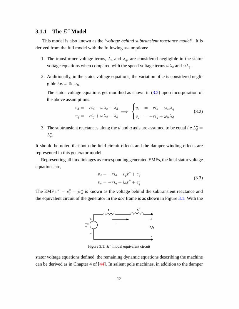
3.1.1 The E ′′ Model
This model is also known as the‘voltage behind subtransient reactance model’. It is
derived from the full model with the following assumptions:
1. The transformer voltage terms,λd and λq, are considered negligible in the stator
voltage equations when compared with the speed voltage termsωλd andωλq.
2. Additionally, in the stator voltage equations, the variation of ω is considered negli-
gible i.e. ω ∼= ωR.
The stator voltage equations get modified as shown in (3.2) upon incorporation of
the above assumptions.
vd = −rid − ωλq − λd
vq = −riq + ωλd − λq
=⇒
vd = −rid − ωRλq
vq = −riq + ωRλd
(3.2)
3. The subtransient reactances along thed andq axis are assumed to be equali.e.L′′
d =
L′′
q .
It should be noted that both the field circuit effects and the damper winding effects are
represented in this generator model.
Representing all flux linkages as corresponding generated EMFs, the final stator voltage
equations are,
vd = −rid − iqx′′ + e′′d
vq = −riq + idx′′ + e′′q
(3.3)
The EMFe′′ = e′′q + je′′d is known as the voltage behind the subtransient reactance and
the equivalent circuit of the generator in theabcframe is as shown in Figure3.1. With the
Figure 3.1:E′′ model equivalent circuit
stator voltage equations defined, the remaining dynamic equations describing the machine
can be derived as in Chapter 4 of [44]. In salient pole machines, in addition to the damper
12

winding, a fictitious short circuited winding is assumed to be present on theq axis to
mimic the field circuit winding in thed axis.
The final equations obtained as are given below:
λD =1
τ ′′d0
√3E ′
q −1
τ ′′d0λD +
1
τ ′′d0(x′
d − xℓ) id (3.4)
√3E ′
q =
√3
τ ′d0EFD +
(xd − x′
d) (x′′
d − xℓ)
τ ′d0 (x′
d − xℓ)id −
√3
τ ′d0
[
1 +(xd − x′
d) (x′
d − x′′
d)
(x′
d − xℓ)2
]
E ′
q
+(xd − x′
d) (x′
d − x′′
d)
τ ′d0 (x′
d − xℓ)2
λD
(3.5)
λQ =−1
τ ′′q0
√3E ′
d −1
τ ′′q0λQ +
1
τ ′′q0
(
x′
q − xℓ
)
iq (3.6)
√3E ′
d =−(
xq − x′
q
) (
x′′
q − xℓ
)
τ ′q0(
x′
q − xℓ
) iq −√3
τ ′q0
[
1 +
(
xq − x′
q
) (
x′
q − x′′
q
)
(
x′
q − xℓ
)2
]
E ′
d
−(
xq − x′
q
) (
x′
q − x′′
q
)
τ ′q0(
x′
q − xℓ
)2λQ
(3.7)
2Hω = Tm − e′′q iq/3− e′′did/3−Dω (3.8)
δ = ω − 1 (3.9)
These differential equations are supported by the following algebraic equations
e′′q =x′′
d − xℓ
x′
d − xℓ
√3E ′
q +x′
d − x′′
d
x′
d − xℓ
λD (3.10)
e′′d =x′′
q − xℓ
x′
q − xℓ
√3E ′
d −x′
q − x′′
q
x′
q − xℓ
λQ (3.11)
This simplified model is the most detailed model used in powersystem transient stability
simulations and its model name in PSLF is GENROU.
3.1.2 The E ′ Model
While the previous model accounted for the subtransient circuit effects, this model
considers those effects as negligible. The remaining two assumptions with regard to the
transformer voltages and the variation ofω still hold for the two axis model.
With the absence of the subtransient circuit, this model is also known as the‘voltage
behind transient reactance model’. The equivalent circuit for the model is as shown in
13

Figure3.2. As a further approximation, the model can be represented asa voltage behind
Figure 3.2:E′ model equivalent circuit
the d axis transient reactance. The detailed reasoning behind this approximation along
with the complete derivation of the dynamic equations can beobtained from Chapter 4
of [44].
The final dynamic equations are as given below:
E ′
q =1
τ ′d0
(
EFD − E ′
q + (xd − x′
d) Id)
(3.12)
E ′
d =1
τ ′q0
(
−E ′
d −(
xq − x′
q
)
Iq)
(3.13)
2Hω = Tm −(
E ′
dId + E ′
qIq)
+(
L′
q − L′
d
)
IdIq −Dω (3.14)
δ = ω − 1 (3.15)
3.1.3 Classical Model
This is the most simple model for the synchronous machine. The significant assump-
tions made for the development of this model are as given below:
1. The air gap flux is constant. Thus the effects of armature reaction are neglected.
2. The voltage behind the transient reactance is constant.
3. The motion of the rotor of the machine coincides with the angle of the voltage behind
the transient reactance.
4. No damper windings exist.
5. Input mechanical powerPm is constant.
Since constant flux constant voltage is assumed, no excitation system can be used for a
generator represented by this model. Further, since the motion of the mechanical rotor
14

angle is assumed to coincide with the internal voltage angle, no governor model can be
used with this machine representation.
The equations representing this model are as given below:
2Hω = Pm − Pe (3.16)
δ = ω − 1 (3.17)
where,Pe is the electrical power injected into the network at the terminals of the machine.
The value of this quantity can be obtained by using the network admittance matrix. In
PSLF, this model goes by the name of GENCLS.
In simulations it is common to take one synchronous machine as the reference machine.
This is done to avoid the dependency of the rotor anglesδ on each other. Thus the angular
velocity differential equations (dδ/dt) are written using relative angles instead of absolute
angles.
3.2 Governor Model
The main function of a governor is to vary the input power to the generator in accor-
dance to the variation in frequency. While governors may have additional tasks depending
on the type of fuel used, the main operational loop of all governors remains similar. To
bring about primary frequency response, a droop controlleris made use of in governors.
The operational characteristic of droop controllers is as shown in Figure3.3. At the rated
Figure 3.3: Droop characteristic
frequency ofωs = 1.0pu the output of the generator is the scheduled powerPg. With a
drop in frequency, the characteristic makes the governor increase the active power thereby
arresting the fall in frequency. Eventually a steady state frequencyωp is attained with an
increased power output ofP ′
g.
15

Based on this characteristic, a simple governor model can bederived as shown in Figure
3.4. The differential equations describing the dynamic behavior of this governor are as
given by (3.18)-(3.20).
Figure 3.4: Governor based on droop characteristics
ds1dt
=1
TG
[
Pref −∆ω
R− s1
]
(3.18)
ds2dt
=1
T2
[
s1 − s2 − s1T1
T2
]
(3.19)
Pm = s2 + s1T1
T2
(3.20)
In PSLF, a governor model very similar to this model is present under the model name of
TGOV1.
3.3 Static Exciter Model
Any realistic generator model,E ′′ or two axis model, has to have an associated ex-
citation system model to represent the exciter. While a handful of generators across the
system continue to have a DC exciter, the static exciter and the brushless AC exciter are
the most common exciters nowadays.
The basic framework of a static exciter model is shown in Figure3.5with the dynamic
equations given by (3.21)-(3.26).ds1dt
=1
Tr
(Vt − s1) (3.21)
e = Vref − s1 − f (3.22)
ds2dt
=1
Tb
[
e− s2 − eTc
Tb
]
(3.23)
ds3dt
=dE
dt=
1
Ta
[
Ka
[
s2 + eTc
Tb
]
− E
]
(3.24)
16

Figure 3.5: Static exciter basic framework
ds4dt
=1
Tf
[−Kf
Tf
E − s4
]
(3.25)
f = s4 + EKf
Tf
(3.26)
In AC and DC exciters, the signalE is the input excitation to the exciter and the armature
voltage of the exciter becomes the input excitation to the synchronous machine. In static
exciters, the signalE can be directly applied as the input excitation to the synchronous
machine field winding and under these circumstances, this signal can be denoted asEFD.
In PSLF, the AC and static exciters models EXAC4 and EXST1 areused.
3.4 Load Model
While nonlinear loads are represented by differential equations depicting their dynamic
behavior, static loads have been traditionally represented by either anexponentialmodel or
a polynomialmodel. Both models can represent a load as either constant power, constant
current or constant impedance. Usually a complex mix of all three types of load are present
in the system at any given point in time. However, if for some reason no detailed load
information exists, then active power loads are represented as constant current loads while
reactive power loads are represented as constant impedanceloads [16].
Often even active power loads are represented as constant impedance loads. With this
representation, all static loads can be absorbed into the system admittance matrix [44].
The current injection into the network now comes from only those components that have
been represented by dynamic equations. The load buses can now be eliminated from the
network equations using matrix reduction techniques [44].
17

Since all generator models are representative of a voltage behind reactance model, the
generator reactance too can be absorbed into the admittancematrix and thereby represent
the generator internal bus as being directly hooked onto thenetwork.
3.5 Network Model
While running a power flow algorithm, the slack bus angle is usually set to zero and
taken as the reference for all other bus angles. In dynamic simulations the slack bus
voltage phasor is considered to coincide with theQ axis of the synchronously rotating
network frame of reference with theD axis leading theQ axis by90◦.
The network equations of (3.1) i.e. g (x, y) = 0 describe the transmission network in
relation to the bus quantities and injections as given by (3.27) & (3.28).
I = Y V (3.27)
where,
I ,
I1
I2
...
In
andV ,
V 1
V 2
...
V n
(3.28)
To complete Ohm’s law,Y is the reduced admittance matrix of the network.
Since a network reduction has already been performed,I andV are vectors of length
nx1wherein it is assumed that there aren buses in the system at which a device is present
with its behavior described by a set of differential equations. Correspondingly, the matrix
Y is of sizenxn. When each phasor ofI, V andY is projected into its components onto
theDQ frame, then the length of the vectors become2nx1while the size of the reduced
admittance matrix becomes2nx2n.
Each synchronous machine is said to have adqaxis which rotates in synchronism with
the rotor of that machine [45]. Due to the different loading levels of each machine, thedq
axis of any particular machine will be displaced from the network DQ axis by an angle
equal to the torque angleδ of that particular machine. Figure3.6shows the displacement
between the two reference frames for any individual machinei. The relationship between
the network and machine frame quantities, as given by (3.29), can be easily obtained by
inspection of Figure3.6.
VQi + jVDi = (Vqi cos δi − Vdi sin δi) + j (Vqi sin δi + Vdi cos δi)
⇒ VD,Q = Vd,qejδi
(3.29)
18

Figure 3.6: Machine and network reference frames for machine i
Therefore, (3.27) can now we rewritten as,
ID,Q = Y VD,Q ⇔ VD,Q = Y −1ID,Q (3.30)
Since the aim of a dynamic simulation is to observe the behavior of the devices connected
to the network, it is preferred that the machine reference frame is maintained throughout
the simulation. Thus (3.30) has to be converted from the network frame to the machine
frame. The procedure as given in [44] is discussed below.
Using the transformation factor defined in (3.29), a transformation matrixT can be
formed for the entire network. Since the transformation factor for each bus is independent
of the other buses, the matrixT will be a diagonal matrix of sizenxnas given,
T =
ejδ1 0 ... 0
0 ejδ2 ... 0
... ... ... ...
0 0 ... ejδn
T−1 =
e−jδ1 0 ... 0
0 e−jδ2 ... 0
... ... ... ...
0 0 ... e−jδn
(3.31)
The vector of voltages in the network and machine frame of reference is given by,
VD,Q =
VQ1 + jVD1
VQ2 + jVD2
...
VQn + jVDn
Vd,q =
Vq1 + jVd1
Vq2 + jVd2
...
Vqn + jVdn
(3.32)
Using the transformation matrixT, the two voltage vectors can be related as
VD,Q = TVd,q
Vd,q = T−1VD,Q = T ∗VD,Q
(3.33)
19

Similar equations can be written to relate the current vectors of both frames of reference.
To transform (3.30), the relations in (3.33) are used.
ID,Q = Y VD,Q =⇒ TId,q = Y TVd,q (3.34)
Upon premultiplying byT−1,
Id,q =(
T−1Y T)
Vd,q , MVd,q ⇔ Vd,q = M−1Id,q (3.35)
where,
M ,(
T−1Y T)
(3.36)
Thus (3.35) gives the desired relation between the currents and voltages of each device
connected by the network, in the machine frame of reference.
If each device is represented as a Thevenin source, then thesolution of the differential
equations will give the values of the voltage vector of (3.35). In order to proceed to the
next time step, (3.35) is now solved to obtain the values of the current vector. These new
values of the current vector are then used in the next time step to obtain the solution of the
differential equations. If the devices are represented as Norton sources, then the solution
of the differential equations would return the values of thecurrent vector and (3.35) would
have to be solved to obtain the values of the voltage vector.
Since the transformation matrixT depends on the torque angle of the machine, the
transformation plays an important role in the dynamic simulation.
In the following chapter, the modeling of the converters andtheir corresponding control
strategies will be discussed.
20

4. Modeling of Converters
The previous chapter discussed the mathematical modeling aspects of the‘conven-
tional’ power system. Recently, due to the increasing addition of renewable sources of
energy, converter models are being included into all commercial software. These models
however differ in complexity from one software vendor to another. In addition, the de-
velopment of generic models had been stalled for quite some time due to non negotiable
proprietary information held by the manufacturers. In PSLF, the converter models and
their associated control models are mainly representativeof GE’s converter models for
wind and solar applications [2,3,46], though, some manufacturer independent wind mod-
els also exist. The basic framework of connecting a converter based source to the grid in
PSLF is as shown in Figure4.1[2] for a solar photovoltaic source and in Figure4.2[3] for
a wind turbine-generator.
Figure 4.1: Modeling solar photovoltaic plants in PSLF [2]
4.1 The Converter Model in Commercial Software (pv1g,gewtg )
The converter is the interface between the source of power and the network. In PSLF,
the modelspv1gandgewtgrepresent the converter model for solar photovoltaic and wind
applications respectively. There is minimal difference between the two models. Figure4.3
shows the block diagram of this converter model [4]. In PSLF, the converter is represented
as a current source which injects the required current into the network. The active and
21

Figure 4.2: Modeling wind turbine-generators in PSLF [3]
reactive current commands are issued from the control block. The model receives the
individual current commands and injects a complex current into the network. The 20ms
time constant represents the switching of the solid state switches within the converter.
Apart from representing the switching action of the converter, built into this block is the
behavior of few limiting devices. The low voltage power logic (LVPL) uses the terminal
voltage to control the upper limit on the active power injected. If the bus voltage of the
converter falls below a certain value, due to the occurrenceof a disturbance, the LVPL
block will reduce the upper limit as per the characteristic shown. Within a range of low
voltage values, the active current upper limit is varied in alinear fashion. If the voltage
falls below the lower boundary of the range, the active current upper limit is made zero.
In the normal operating voltage range, the LVPL block does not affect the active current
upper limit. All settings in the LVPL block can be set by the user.
Further, two algebraic current limiters are present in thisblock. Thehigh voltage reac-
tive current managementsection is instrumental in reducing the reactive power injected if
the terminal voltage rises above a certain user defined limit. The user also has the freedom
to set the rate at which the reactive power is ramped down. Thelow voltage active current
managementsection takes care of reducing the active power injected while the voltage
falls below a certain value. Its function is similar to the LVPL block.
22

Figure 4.3: Converter model in PSLF [4]
4.2 The Converter Control Model in Commercial Software
(pv1e,ewtgfc)
The control model is responsible for generating the active and reactive current com-
mands for the converter model. The block diagram of this model is depicted in Figure
4.4[4]. The bottom section of the model shows the calculation of the active current com-
mand. The reference active power,Pord, can be either set by the user using an external
user-written dynamic model or the value scheduled in the power flow. This feature thus
allows for the inclusion of a governor type model to set the active power as will be shown
later on in this report.
The model allows for three different ways of setting the reactive current command.
These various modes can be toggled using thevarflg parameter as shown in the block
diagram. These different ways are:
1. PV VAr controller emulator: This emulator is nothing but avoltage regulator. The
terminal voltage is compared to its reference value and the desired amount of reac-
tive power is calculated using a PI controller.
2. Power factor regulator: The converter can be operated at adesired power factor and
the reactive power is calculated based on the required powerfactor and the active
23

Figure 4.4: Converter control model in PSLF [4]
power.
3. User defined reactive power: The user has an option to provide a value of required
reactive power.
The converter current limit block ensures that all current commands are within certain
limits. The details of the operation of this limiter are provided in [2].
4.3 User Defined Converter Control Model
While the control model described in the previous section was found to work as per
design and specifications, it was deemed to be complex. With the aim of achieving close
to 100% CIG penetration, a requirement arises for simpler control structures bearing in
mind that the stability of the system hinges upon the interaction of these controls with one
24

another. In addition, as different manufacturers would have their own variation of control
architecture, a simple control was used to focus on the modelof the converter. With this
objective, a controller as shown in Figure4.5was designed for the converter.
(a) Reactive power controller
(b) Real power controller
Figure 4.5: User defined converter control model
The effective real power order (Figure4.5(b)) is a combination of the power setpoint
and the active power droop coefficient while the reactive power order (Figure4.5(a)) is
obtained from the voltage error along with a reactive power droop. The QV droop is
instrumental in obtaining a stable operation between converters when multiple converters
are connected to the same bus. The active power droop coefficient is denoted asRp and the
reactive power droop coefficient is denoted asRq. The equations describing the behavior
of the controller are given by (4.1) to (4.5).ds1dt
= Ki [Vref − s2 − RqQg] (4.1)
ds2dt
= (1/Tr) ∗ [Vt − s2] (4.2)
ds3dt
= (1/TGpv) ∗ [Pref − (∆ω/Rp)− s3] (4.3)
25

Qcmd = s1 +Kp [Vref − s2 − RqQg] (4.4)
Pcmd = s3 (4.5)
Limits have been imposed on the maximum active and reactive power and minimum
reactive power deliverable. In choosing the limits for the reactive and active power, it
has been assumed that the converter can withstand an instantaneous MVA of 1.7 times its
rating. Further, it has been assumed that at a terminal voltage level of 0.75pu, the minimum
operable power factor is 0.4. As the voltage dips, the limitsof the converter control will
change to allow for more reactive power to be delivered whilecurtailing the active power
delivered to meet the MVA rating. Though a terminal voltage of 0.75pu has been chosen
as the minimum voltage, the maximum deliverable reactive power is maintained constant
for voltages below 0.8pu as shown in Figure4.6. The value ofqmax1is taken from the
Figure 4.6: Variation ofQlimit with Vt
power flow but is assumed to be the value of maximum reactive power at a voltage level
of 1.0pu. The value ofqmax2is obtained as given by (4.6).
qmax2=
√
(1.7 ∗MVA)2
1 +(
1
tan cos−1 0.4
)2(4.6)
Therefore, at any voltage levelVt above 0.8pu, the value ofqmax is obtained as given by
(4.7).
qmax = qmax1+
qmax2− qmax1
0.8− 1.0(Vt − 1.0) (4.7)
26

The value ofqmin is maintained constant as specified in the power flow while themaximum
active power is obtained as in (4.8) to maintain the MVA rating.
pmax =√
(1.7 ∗MV A)2 − q2max (4.8)
Since an integrator is present in the reactive power loop, the windup limit has been
converted to an anti-windup limit as per the scheme mentioned in [47]. The block diagram
of this conversion is as shown in Figure4.7 where the value ofKlimit is appropriately
chosen.
Figure 4.7: Conversion from windup to anti-windup limit
To model the converter, a voltage source representation of the converter has been pro-
posed in this research work. The voltage source representation has first been modeled at
the electromagnetic transient level using the PLECS [48] software package. This model-
ing has then been used as a basis for the development of a positive sequence phasor model
which is required for large scale grid simulation. Using thePLECS software package, a
detailed switching model of the converter has been simulated. The control mechanism
described in Figure4.5 is used to generate the current commands which are then used
as shown in Figure4.8 to generate the reference voltage wave to obtain the pulse width
modulated signals. A 5 microsecond time step has been used for the simulation. The fast
inner current control loops are required in the electromagnetic transient simulation to ob-
tain the magnitude and phase angle of the PWM reference voltage wave. This detail of
modeling the voltage source converter and its control is however not suitable for the simu-
lation of large networks as it would require a smaller time step of simulation to accurately
capture the inner loop behavior and this would considerablyincrease the time duration of
simulation.
Due to the effect of grid impedance on the operation of the inner current control loop
[49], a wide variety of inner current control loops are used in practical inverters with the
27

Figure 4.8: Inner current control loop in PLECS to generate PWM reference voltage wave
common characteristic of response times that are very fast in relation to the bandwidth
proposed for grid level controls. Accordingly, the grid level modeling used in this project
represents the behavior of the inner control loops by simpletime constants. Hence, two
alternatives can be considered for modeling the convertersin positive sequence:
• With the assumption that the inner current control loop is very quick, the converter is
modeled as a specified current boundary condition on the positive sequence network
solution model. This representation has been referred to asthe boundary current
representation wherein the values ofiq and id from Figure4.10 are the boundary
currents as shown in Figure4.9.
• As the converter is a voltage source converter with a voltage source on the dc side,
the converter is modeled as a Thevenin voltage source described by Figure4.10and
(4.9) and the active power controller is modeled as shown in Figure4.11.
Figure 4.9: Boundary current converter representation forpositive sequence simulation
28
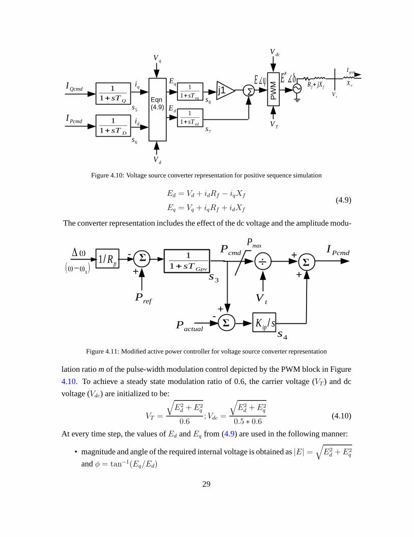
Figure 4.10: Voltage source converter representation for positive sequence simulation
Ed = Vd + idRf − iqXf
Eq = Vq + iqRf + idXf
(4.9)
The converter representation includes the effect of the dc voltage and the amplitude modu-
Figure 4.11: Modified active power controller for voltage source converter representation
lation ratiomof the pulse-width modulation control depicted by the PWM block in Figure
4.10. To achieve a steady state modulation ratio of 0.6, the carrier voltage (VT ) and dc
voltage (Vdc) are initialized to be:
VT =
√
E2d + E2
q
0.6;Vdc =
√
E2d + E2
q
0.5 ∗ 0.6 (4.10)
At every time step, the values ofEd andEq from (4.9) are used in the following manner:
• magnitude and angle of the required internal voltage is obtained as|E| =√
E2d + E2
q
andφ = tan−1(Eq/Ed)
29

• The modulation index is calculated asm = |E|/VT . The value ofm is limited to be
between 0.4 and 1.0.
• The phase voltage values are then obtained asEa,b,c = 0.5mVdc cos(ωst+φ− 120i)
whereωs is 377rad/s andi = 0, 1, 2
• value ofE∗
d andE∗
q (E∗∠δ) is obtained by applying Park’s transformation onEa,b,c.
A lower steady state modulation ratio will require a higher dc voltage magnitude to main-
tain the same ac voltage and would restrict the lower band gapof the modulation ratio.
A steady state modulation ratio of 0.6 has been chosen to allow for a sufficient range of
values for the transient modulation ratio.
In addition, two protection schemes have been incorporated:
• As the converters have a hard current limit, an instantaneous overcurrent protection
has been implemented with a cut-off current of 1.7 pu [2].
• A time dependent overvoltage protection has also been implemented. If the voltage
at the terminalVt rises 0.15 pu more than the steady state voltage for more than0.1s,
the converter is tripped.
The implementation of this converter and its associated controller for positive sequence
time domain simulation was carried out in PSLF [50] by writing an EPCL code as given
in AppendixA. EPCL is PSLF’s in-built programming language.
4.4 Induction Motor Drive Model
The need for precise speed control of induction motors has resulted in the development
of speed control power electronic drives. In a futuristic grid, both the generation source
and the loads could be interfaced through converters. It is thus important to simultaneously
develop positive sequence models for converter interfacedloads.
The equations representing the induction motor are as developed in [16] given here by
(4.11)-(4.13). As a squirrel cage induction motor is assumed to be used, the rotor side
equations of the machine are not present and only the stator equations are required along
with the swing equation of the machine.dωrind
dt=
1
2Hind
(Tm − Te) (4.11)
T ′
o
dv′ddt
= −v′d −X2
m
Xr
iqs +sXrv
′
q
Rr
(4.12)
30

T ′
o
dv′qdt
= −v′q +X2
m
Xr
ids −sXrv
′
d
Rr
(4.13)
The control diagram of the speed control drive model is shownin Figure4.12[51]. The
Figure 4.12: Control diagram of induction motor speed control drive
rectifier for the drive was considered to be an uncontrolled full bridge diode rectifier while
the sinusoidal pulse-width modulation reference signal, denoted byV refs andωref
s , was
generated to maintain constant flux inside the motor and maintain a constant rotor speed
of ωrefr .
In the following chapter, a discussion of the results verifying the performance of this
converter control for various system configurations and theinduction motor drive model
is recorded.
31

5. Simulation and Results
The performance of the converter and its associated controlwas first validated with the
performance of the converter in PLECS by using a simple test system. Following this, the
performance of the converter was analyzed in a 3 generator system and the 2012 WECC
system.
5.1 Converter Model Validation in a Two Machine System
A C code was written to simulate the time domain dynamic response of the converter
representation shown in Figures.4.5 and4.10. A simple test system as shown in Figure
5.1was constructed to compare the behavior of the converter model in positive sequence
with its behavior in PLECS. The loads were treated as constant admittance loads. For the
Figure 5.1: Two machine system
simulation, the synchronous machine was represented by a round rotorgenroumodel with
an inertia constantH = 2.2s along with an associated governor and static exciter model.
To observe the response of the converter, an additional 8MW was switched on att = 1s at
bus 2. Following this, att = 1.1s, the reference command to the converter (Pref in Figure
4.5(b)) was changed from 0MW to 8MW.
In the PLECS simulation, a 5 kHz switching frequency was usedto obtain the pulse
width modulated waveform. The reactive power loop had gainsof 4.0 and 20.0 respec-
32

tively for the proportional and integral controllers in both PLECS and the positive se-
quence simulation. The active power integral controller inthe positive sequence simula-
tion had a gain of 0.5.
The comparison between the PLECS simulation and the positive sequence model is
shown by the active power output of the converter in Figure5.2. Further, Figures.5.3and
5.4show the 3 phase voltage and current waves at the converter terminals. From these fig-
ures it can be seen that the response of the converter is completed in approximately 50ms
and the demand is quickly met. However, the positive sequence response differs from
0 0.5 1 1.5 2 2.5 3 3.5 4 4.5 5−2
0
2
4
6
8
10
12
Time (s)
Pow
er (
MW
)
PLECSPositive Sequence
0.8 1 1.2 1.4 1.6 1.8 2
0
2
4
6
8
10
Time (s)
Pow
er (
MW
)
PLECSPositive Sequence
Figure 5.2: Comparison of the converter active power outputbetween PLECS and positive sequencesimulation
the PLECS model response at the instant of disturbance. One reason for this difference is
the fact that in PLECS, a differential equation model is usedto depict the filter inductors
of the converter whereas in the positive sequence model, thefilter inductor is represented
algebraically as a simple reactance. Hence the PLECS response to a disturbance shows a
small finite time constant as opposed to the instantaneous response obtained from the pos-
itive sequence simulation. This representation of the inductor is required for the point on
wave type of simulation carried out in PLECS whereas the phasor simulation is unable to
represent this feature. Secondly, as the PLECS simulation works on instantaneous values
of voltage and current, a phased locked loop is required to track the phase angle of the
voltage at the converter terminal and a small time constant is associated with this tracking.
As expected, the response of the converter to the step changein Pref is completed
33

0.95 1 1.05 1.1 1.15 1.2 1.25−600
−400
−200
0
200
400
600
Time (s)
Vol
tage
(V
)
Figure 5.3: Phase voltage waveforms at the converter terminal from PLECS
0.95 1 1.05 1.1 1.15 1.2 1.25−1.5
−1
−0.5
0
0.5
1
1.5x 10
4
Time (s)
Cur
rent
(A
)
Figure 5.4: Line current waveforms at the converter terminal from PLECS
in approximately 50ms. The 0.1s delay in triggering the change in reference command
is used to simulate a transfer trip situation. This scenariotherefore depicts the natural
response of the converter model to a change in the reference command.
The simplified positive sequence model representing the converter as a controlled volt-
34

age source without the explicit representation of the innercurrent control loop shows the
same behavioral trend as the electromagnetic transient simulation. Thus while simulating
large systems, this simplified model can be utilized.
The behavior of the PLL is intertwined with the value of the filter inductor and the gains
of the inner current control loop. In order to restrict the percentage of ripple in the output
current, the value of the filter inductor is decided based on the switching frequency. In
addition, the switching frequency imposes a limit on the current loop bandwidth. Further,
the PLL bandwidth should generally be lower than 60Hz in gridconnected applications.
In this project, the value of the filter inductor was so chosenas to restrict the current ripple
to a maximum of 5%.
The sensitivity of the converter response to the PLL gain is as shown in Figure5.5.
Indirectly, the sensitivity of the converter response to the value of the filter inductor is also
conveyed by the same curve. It can be seen that as the PLL becomes slower (lower gain),
its effect is reflected in the performance of the converter inthe few milliseconds following
the disturbance. For this value of filter inductance, a faster PLL makes the system unstable.
The next section will discuss the implementation of the simplified time domain converter
1 1.5 2 2.5 3−2
0
2
4
6
8
10
12
Time (s)
Pow
er (
MW
)
Original PLL gainHalf PLL gainQuarter PLL gain
Figure 5.5: Converter active power output for different PLLgains
model in commercial positive sequence time domain simulation software.
5.2 Results in Commercial Software
The two positive sequence converter models namely, the boundary current injection
and the voltage source representation of the converter, were implemented with the ‘user
written model’ feature of the large scale grid simulation program PSLF.
35

5.2.1 Small Scale System-Validation of Results
A three machine nine bus equivalent system [44] shown in Figure5.6 was used to
validate the performance of the developed converter controller model in PSLF. This system
Figure 5.6: Three machine nine bus equivalent system
consists of 9 buses, 3 generators and 3 static loads. Though the size of the system is small,
it is sufficient to showcase a variety of stability concepts.The powerflow solution of this
network, power consumed by the load at buses 5, 6 and 8 and the dynamic data is given in
AppendixB.
From the structure of the system it can be seen that any type offault will significantly
affect all three sources. However the purpose of this systemis to analyze the effect of
small disturbances that occur frequently in the power system. The load in a system is
continuously changing and the generation sources have to appropriately adjust their load
setpoints to meet the demand. Thus, the behavior of the converter model to an increase in
load was compared with its behavior in PLECS for the same disturbance.
With the loads treated as constant admittance, the load at bus 6 was increased by 10MW
36
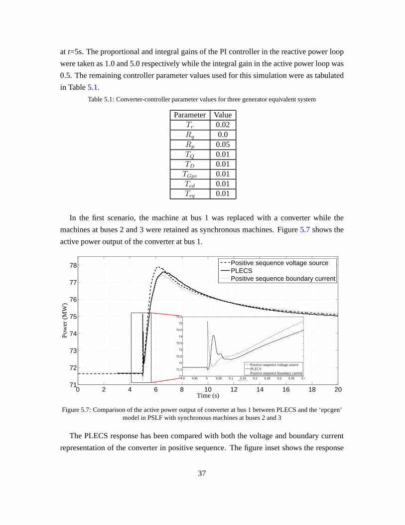
at t=5s. The proportional and integral gains of the PI controller in the reactive power loop
were taken as 1.0 and 5.0 respectively while the integral gain in the active power loop was
0.5. The remaining controller parameter values used for this simulation were as tabulated
in Table5.1.
Table 5.1: Converter-controller parameter values for three generator equivalent system
Parameter ValueTr 0.02Rq 0.0Rp 0.05TQ 0.01TD 0.01TGpv 0.01Ted 0.01Teq 0.01
In the first scenario, the machine at bus 1 was replaced with a converter while the
machines at buses 2 and 3 were retained as synchronous machines. Figure5.7 shows the
active power output of the converter at bus 1.
0 2 4 6 8 10 12 14 16 18 2071
72
73
74
75
76
77
78
Time (s)
Pow
er (
MW
)
Positive sequence voltage sourcePLECSPositive sequence boundary current
4.9 4.95 5 5.05 5.1 5.15 5.2 5.25 5.3 5.35 5.471
71.5
72
72.5
73
73.5
74
74.5
75
75.5
Time (s)
Positive sequence voltage sourcePLECSPositive sequence boundary current
Figure 5.7: Comparison of the active power output of converter at bus 1 between PLECS and the ‘epcgen’model in PSLF with synchronous machines at buses 2 and 3
The PLECS response has been compared with both the voltage and boundary current
representation of the converter in positive sequence. The figure inset shows the response
37
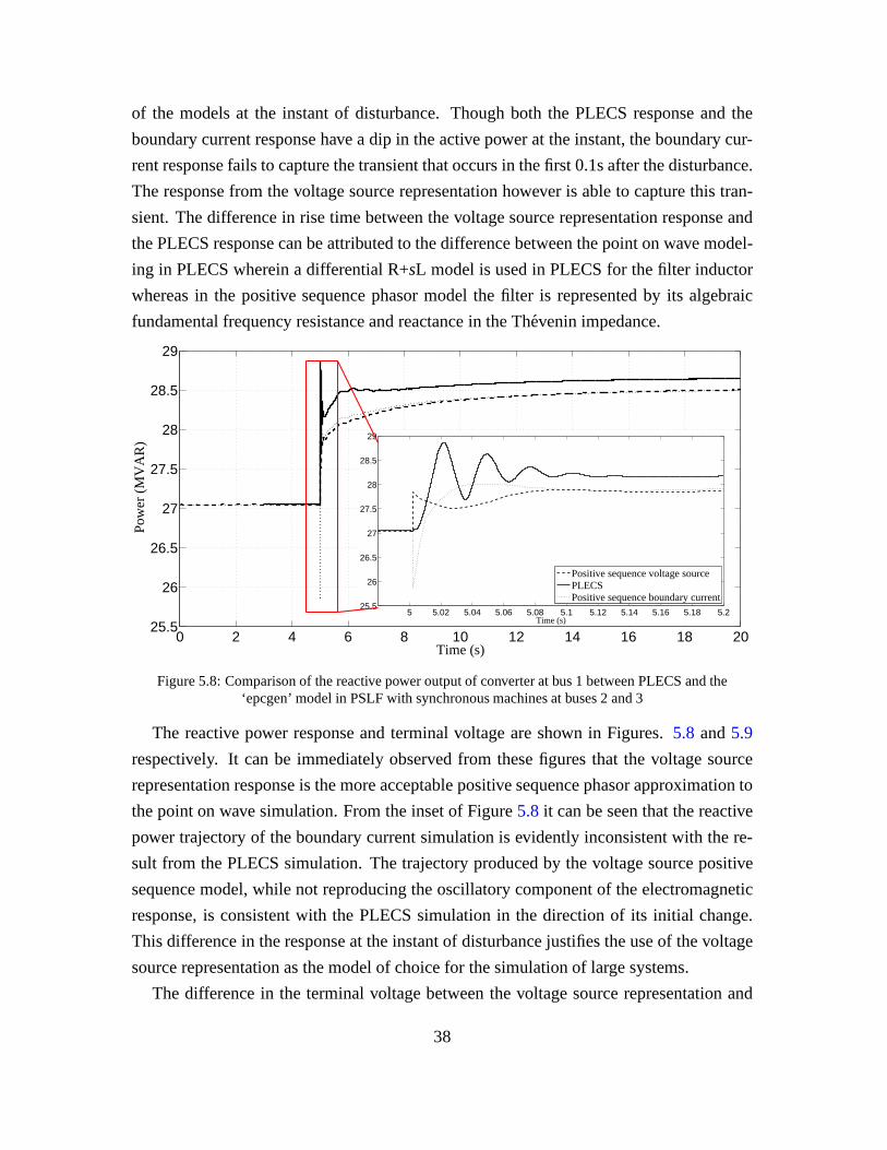
of the models at the instant of disturbance. Though both the PLECS response and the
boundary current response have a dip in the active power at the instant, the boundary cur-
rent response fails to capture the transient that occurs in the first 0.1s after the disturbance.
The response from the voltage source representation however is able to capture this tran-
sient. The difference in rise time between the voltage source representation response and
the PLECS response can be attributed to the difference between the point on wave model-
ing in PLECS wherein a differential R+sL model is used in PLECS for the filter inductor
whereas in the positive sequence phasor model the filter is represented by its algebraic
fundamental frequency resistance and reactance in the Thevenin impedance.
0 2 4 6 8 10 12 14 16 18 2025.5
26
26.5
27
27.5
28
28.5
29
Time (s)
Pow
er (
MV
AR
)
5 5.02 5.04 5.06 5.08 5.1 5.12 5.14 5.16 5.18 5.225.5
26
26.5
27
27.5
28
28.5
29
Time (s)
Pow
er (
MV
AR
)
Positive sequence voltage sourcePLECSPositive sequence boundary current
Figure 5.8: Comparison of the reactive power output of converter at bus 1 between PLECS and the‘epcgen’ model in PSLF with synchronous machines at buses 2 and 3
The reactive power response and terminal voltage are shown in Figures.5.8 and5.9
respectively. It can be immediately observed from these figures that the voltage source
representation response is the more acceptable positive sequence phasor approximation to
the point on wave simulation. From the inset of Figure5.8 it can be seen that the reactive
power trajectory of the boundary current simulation is evidently inconsistent with the re-
sult from the PLECS simulation. The trajectory produced by the voltage source positive
sequence model, while not reproducing the oscillatory component of the electromagnetic
response, is consistent with the PLECS simulation in the direction of its initial change.
This difference in the response at the instant of disturbance justifies the use of the voltage
source representation as the model of choice for the simulation of large systems.
The difference in the terminal voltage between the voltage source representation and
38

0 2 4 6 8 10 12 14 16 18 201.03
1.032
1.034
1.036
1.038
1.04
1.042
Time (s)
Vol
tage
(pu
)
4.95 5 5.05 5.1 5.15 5.2 5.251.03
1.032
1.034
1.036
1.038
1.04
Time (s)
Positive sequence voltage sourcePLECSPositive sequence boundary current
Figure 5.9: Comparison of the terminal voltage of converterat bus 1 between PLECS and the ‘epcgen’model in PSLF with synchronous machines at buses 2 and 3
the boundary current representation at the instant of disturbance can be attributed to the
presence of the filter inductor. In both the voltage source representation and the PLECS
response, the presence of the filter inductor provides a connection to ground and thereby
reduces the voltage dip as can be seen from Figure5.9.
The sensitivity of the terminal voltage to the value of the filter inductor is as shown
in Figure5.10. It can be seen that as the per unit value of the filter inductorincreases,
the nadir of the terminal voltage decreases. The boundary current representation of the
converter is akin to a voltage source representation with a very high value of filter induc-
tance as voltage sources are represented by their Norton equivalent in positive sequence
time domain simulation software. Thus, as the value of the filter inductor increases, the
impedance to ground increases thereby causing a higher voltage drop at the terminal bus.
It could be argued that the nadir of the terminal voltage can be affected by the con-
trol mechanism used for the boundary current source representation. However to achieve
the same nadir as the electromagnetic transient simulationresponse, an exceptionally high
value of control gains would be required. This would howeverstill not represent the first
peak obtained and it could make the control structure unstable. Practically, a wide range
of control techniques for converter interfaced generationexists. The intricacies of the con-
trol structure vary with the type of energy source and the manufacturer of the equipment
used to harness said energy source. These control techniques can however become quite
complicated and since the focus of this research was to be on the representation of the
39

0 2 4 6 8 10 12 14 16 18 201.034
1.035
1.036
1.037
1.038
1.039
1.04
1.041
1.042
Time (s)
Vol
tage
(pu
)
4.95 5 5.05 5.1 5.15 5.2 5.251.034
1.035
1.036
1.037
1.038
1.039
1.04
1.041
Time (s)
Xf = 0.5pu
Xf = 0.3pu
Xf = 0.8pu
Figure 5.10: Sensitivity of the terminal voltage of converter at bus 1 for positive sequence voltage sourcerepresentation to different values of filter inductor
converter, a simplified control structure was used.
In order to look at an all CIG system, the machines at buses 2 and 3 were also replaced
with both forms of the positive sequence converter model. The instantaneous rise in the
active power of the voltage source representation can be calculated on the same lines as
the distribution of impact calculation for synchronous machines.
Based on the electrical distance between the internal voltage source of the converter
and the disturbance point, the instantaneous response of a converter at busi for an impact
at busk can be obtained as:
Pi∆(0+) =
(
Psik/n∑
j=1
Psjk
)
PL∆(0+) i = 1, 2, .., n (5.1)
where
Psik = ViVk (Bik cos δik0 −Gik sin δik0) (5.2)
andPL∆(0+) is the load impact at busk. The entire derivation of (5.1) is available in [44].
Though the PLECS response is not instantaneous, the peak of the first oscillation falls at
around the same value as the instantaneous response as can beseen from Figure5.7. Thus
(5.1) can be used to obtain the approximate peak value of the converter response following
a disturbance.
For the same load increase of 10 MW at bus 6 att=1s, the active power output from
the converters is as shown in Figure5.11 while Figure5.12 shows the reactive power
40

output. With the final steady state values being almost the same, the behavior of the
models at the instant of disturbance becomes the deciding factor. It can be seen that in an
all CIG system too, the boundary current representation response instantaneously moves
in a direction opposite to what would be expected while the response from the voltage
source representation is as expected and it conforms to (5.1).
0 1 2 3 4 5 6 760
70
80
Pow
er(M
W)
Active power at bus 1
Positive sequence voltage sourcePositive sequence boundary current
0 1 2 3 4 5 6 7150
160
170
Pow
er(M
W)
Active power at bus 2
Positive sequence voltage sourcePositive sequence boundary current
0 1 2 3 4 5 6 780
85
90
Pow
er(M
W)
Time(s)
Active power at bus 3
Positive sequence voltage sourcePositive sequence boundary current
Figure 5.11: Active power output of the converters for an allCIG system with increase in active power load
To further compare the two positive sequence converter representations, the reactive
power load at bus 6 was increased by 10MVAR att=1s while the active part remained
unchanged, in an all CIG system. In a synchronous machine, the rotor speed gives an
indication of the network frequency. However since converters are static sources, an ap-
proximate network frequency is obtained by performing a numerical differentiation of the
bus voltage angle. In PSLF, the dynamic modelfmetr performs this task. With the load
change as mentioned, Figure5.13shows the frequency response. This response was ob-
tained at bus 5.
The figure shows a large difference in transient frequency between the two converter
representations. A possible explanation can be as follows:for the boundary current repre-
sentation of the converter, at the instant of disturbance, the bus voltage angles can experi-
ence a step change which upon differentiation can produce a large change in frequency. In
the voltage source representation however, the bus voltageangles does not change drasti-
cally.
41

0 1 2 3 4 5 6 726
28
30
Pow
er(M
VA
R) Reactive power at bus 1
Positive sequence voltage sourcePositive sequence boundary current
0 1 2 3 4 5 6 76
8
10
Pow
er(M
VA
R) Reactive power at bus 2
Positive sequence voltage sourcePositive sequence boundary current
0 1 2 3 4 5 6 7−11
−10
−9
Pow
er(M
VA
R)
Time(s)
Reactive power at bus 3
Positive sequence voltage sourcePositive sequence boundary current
Figure 5.12: Reactive power output of the converters for an all CIG system with increase in active powerload
0 1 2 3 4 5 6 760
60.1
60.2
60.3
60.4
60.5
60.6
60.7
60.8
Time (s)
Fre
quen
cy (
Hz)
Positive sequence voltage sourcePositive sequence boundary current
Figure 5.13: Frequency response of an all CIG system with increase in reactive power load
The plot of the voltage magnitude at the terminals of the converters and at the load bus is
as shown in Figure5.14. It can be seen that the drop in voltage magnitude at the terminals
of the converters is around 0.02pu while the drop at the load bus is around 0.03pu. For a 10
MVAR increase in load, this is a nominal decrease in voltage magnitude and the fast action
42

0 1 2 3 4 5 6 71
1.05
1.1
Vol
tage
(pu
)
Terminal voltage at bus 1
Positive sequence voltage sourcePositive sequence boundary current
0 1 2 3 4 5 6 71
1.02
1.04
1.06
Vol
tage
(pu
)
Terminal voltage at bus 2
Positive sequence voltage sourcePositive sequence boundary current
0 1 2 3 4 5 6 71
1.02
1.04
1.06
Vol
tage
(pu
)
Terminal voltage at bus 3
Positive sequence voltage sourcePositive sequence boundary current
0 1 2 3 4 5 6 70.98
1
1.02
1.04
Time (s)
Vol
tage
(pu
)
Terminal voltage at bus 6
Positive sequence voltage sourcePositive sequence boundary current
Figure 5.14: Voltage magnitudes of an all CIG system with increase in reactive power load
of the converters bring the voltage back to the pre-contingency value within 1s. Due to the
increase in load, the voltage at the load bus is lower, as expected. The change in active and
reactive power of the converters are shown in Figures5.15and5.16respectively.
0 1 2 3 4 5 6 766
68
70
72
Pow
er (
MW
)
Active Power at bus 1
Positive sequence voltage sourcePositive sequence boundary current
0 1 2 3 4 5 6 7155
160
165
Pow
er (
MW
)
Active Power at bus 2
Positive sequence voltage sourcePositive sequence boundary current
0 1 2 3 4 5 6 780
82
84
86
Time (s)
Pow
er (
MW
)
Active Power at bus 3
Positive sequence voltage sourcePositive sequence boundary current
Figure 5.15: Active power output of the converters for an allCIG system with increase in reactive powerload
It has thus been established that the voltage source representation of the converter is the
43

0 1 2 3 4 5 6 726
28
30
32
34
Pow
er (
MV
AR
)
Reactive Power at bus 1
Positive sequence voltage sourcePositive sequence boundary current
0 1 2 3 4 5 6 76
8
10
12
Pow
er (
MV
AR
)
Reactive Power at bus 2
Positive sequence voltage sourcePositive sequence boundary current
0 1 2 3 4 5 6 7−11
−10
−9
−8
−7
Time (s)
Pow
er (
MV
AR
)
Reactive Power at bus 3
Positive sequence voltage sourcePositive sequence boundary current
Figure 5.16: Reactive power output of the converters for an all CIG system with increase in reactive powerload
more appropriate representation in positive sequence phasor simulations of large systems.
5.2.2 Large Scale System-Economy of Computation
To ensure that this model is practical in a large scale system, the WECC 2012 system
has been used. At this stage, it is important to test the robustness and numerical behavior
of the model when large number of converters are present in the system. This system has
18205 buses, 13670 lines and 3573 generators. The total generation is 176 GW while the
total load is 169 GW. The power flow diagram of the system is as shown in Figure5.17[5].
To obtain a sizable presence of converters, all the generators in the Arizona and Southern
California area (528 units) were replaced with converters represented by the proposed
voltage source representation. This accounted for 24.3% ofthe total system generation
with 25.6 GW in Arizona and 17 GW in Southern California.
For a CIG to take part in frequency regulation, a reserve margin has to be present. As
per the associated material for the WECC system operating case [5], all areas of the sys-
tem have a defined amount of headroom available for frequencyregulation. This reserve
is however not distributed equally among all generators in the area, with few generators
operating without a governor. In this project, the maximum active power deliverable by a
CIG unit has been assumed to be equal to the MW rating of the turbine of the generator
which the CIG replaces while the MVA rating of the CIG has beenassumed to be the
44

Figure 5.17: Power flow in the WECC system [5]
45

same as the MVA rating of the generator. If the CIG replaces a generator without an asso-
ciated governor, then it has been assumed that the CIG too cannot take part in frequency
regulation.
Thus, with an available headroom on almost all converter interfaced sources, the value
of the droop coefficientRp was taken to be the same as that used by the governor of the
synchronous machine it replaced whileRq was taken to be 0.05pu on a machine MVA
base. The reactive power PI controller gains of all converters were set toKp=1.0 and
Ki=5.0 while the active power integral controller had a gain ofKip=0.5. The values of all
other parameters were kept the same as in Table5.1.
This initial penetration of 24.3% is used to test the numerical stability of the converter
model for three system contingencies.
Generation Outage (24.3% CIG penetration)
At t=15s, two of the Palo Verde units were tripped resulting in a generation outage of
2755 MW. Fig5.18shows the power output from the remaining sources in the Arizona
area while the effect on the adjacent area of Southern California has been shown in Figure
5.19.
0 10 20 30 40 50 602.26
2.28
2.3
2.32
2.34
2.36
2.38
2.4
2.42x 10
4
Time (s)
Pow
er (
MW
)
14.95 15 15.05 15.1 15.15 15.2 15.25 15.3 15.35 15.4 15.452.28
2.3
2.32
2.34
2.36
2.38
2.4
2.42
x 104
Time (s)
Figure 5.18: Active power generation in the Arizona area dueto trip of two Palo Verde units
The system frequency plot is shown in Figure5.20. It can be seen that the reduction in
frequency is quickly arrested due to the fast action of the converters and the system has no
problem in absorbing the substantial CIG presence.
46

0 10 20 30 40 50 601.67
1.68
1.69
1.7
1.71
1.72
1.73
1.74
1.75
1.76x 10
4
Time (s)
Pow
er (
MW
)
Figure 5.19: Total generation in Southern California area due to trip of two Palo Verde units
0 10 20 30 40 50 6059.84
59.86
59.88
59.9
59.92
59.94
59.96
59.98
60
60.02
Time(s)
Fre
quen
cy(H
z)
Figure 5.20: System frequency due to trip of two Palo Verde units
In terms of computation time, PSLF took 7:04 minutes to run this 60 second simulation
with the first 20 seconds of simulation taking 1:52 minutes. In comparison to this, when
all machines were represented in the conventional manner, the same 60 second simulation
took 6:41 minutes with the first 20 seconds of simulation being completed in 1:39 minutes.
Both simulations were run on a machine with an i7 processor and 16.0 gb of RAM with a
simulation time step of 0.0041s.
47

Line Fault followed by Outage (24.3% CIG penetration)
A three phase fault was applied on a tie line between Arizona and Southern California at
t=15s. Subsequently, att=15.1s, the breakers at both ends of the line were opened. The
initial flow on the line was 1408.6 MW and 134.4 MVAR from the Arizona side. Figures.
5.21, 5.22and5.23show the changes in the power transfer between Southern California
and the areas of Arizona, Los Angeles Department of Water andPower (LADWP) and
San Diego. Negative values indicate that the power flow is into Southern California while
positive values indicate power flow out of the region. The opening of the line causes a
reduction in flow between Arizona and Southern California asexpected.
0 10 20 30 40 50 60−2600
−2400
−2200
−2000
−1800
−1600
−1400
−1200
−1000
−800
Time(s)
Pow
er (
MW
)
Figure 5.21: Active power flow to Southern California from Arizona with the opening of a tie line betweenArizona and Southern California following a line fault
It should be noted that only the voltage source representation of the converter was
able to function reliably following the fault. The boundarycurrent representation of the
converters resulted in frequent non convergence issues with regard to the network solution
following the occurrence of the fault.
Bus Fault (24.3% CIG penetration)
The third contingency carried out on the WECC system was applying a bus fault for 0.1s
at t=15s near the Four Corners generation plant in the Arizona area. The active power
and terminal voltage of one of the units is as shown in Figures. 5.24and5.25. From the
active power plot the familiar damped rotor angle oscillations can be observed from the
output of the synchronous machine. In addition, it can also be seen that a large electronic
48

0 10 20 30 40 50 60−4500
−4000
−3500
−3000
−2500
−2000
Time(s)
Pow
er(M
W)
Figure 5.22: Active power flow to Southern California from LADWP with the opening of a tie line betweenArizona and Southern California following a line fault
0 10 20 30 40 50 60100
200
300
400
500
600
700
800
Time(s)
Pow
er(M
W)
Figure 5.23: Active power flow from Southern California to San Diego with the opening of a tie linebetween Arizona and Southern California following a line fault
source brings about a highly damped response. However, the voltage dip in the converter
response is larger than that of the corresponding synchronous machine. The value of the
filter inductor along with the absence of a sub-transient capability influences the magni-
tude of this dip in voltage. The magnitude of the converter current for the voltage source
representation is as shown in Figure5.26. The current is well within its short time current
rating of 1.7pu. It has also been observed that for few other significant bus faults, the
49

0 5 10 15 20 25 30180
200
220
240
260
280
300
320
Time (s)
Pow
er (
MW
)
Synchronous MachineConverters as voltage source
Figure 5.24: Active power output of a unit at Four Corners fora bus fault close to the unit
0 5 10 15 20 25 300.75
0.8
0.85
0.9
0.95
1
1.05
1.1
Time (s)
Vol
tage
(pu
)
Synchronous MachineConverter as voltage source
14.6 14.8 15 15.2 15.4 15.6 15.8 16 16.20.75
0.8
0.85
0.9
0.95
1
1.05
Time (s)
Vol
tage
(pu
)
Synchronous MachineConverters as voltage source
Figure 5.25: Terminal voltage of a unit at Four Corners for a bus fault close to the unit
network solution diverges when the boundary current representation is used.
The performance of the developed converter model and its associated control structure
has been validated for a large system by these three contingencies. The simulation is
numerically stable and not computationally intensive.
50

0 5 10 15 20 25 300.95
1
1.05
1.1
1.15
1.2
1.25
1.3
1.35
Time (s)
Cur
rent
(pu
)
Figure 5.26: Magnitude of converter current for a voltage source representation of the converter for a busfault close to the unit
5.3 Note on Boundary Current Representation of Converter
In order to study the effect of large penetration of converter interfaced generation in
the power system, it is very important that the computer simulation models have a reliable
representation of the converter. Based on the results of theprevious two sections, it has
been shown that the boundary current representation is not asuitable representation due to
the following reasons:
1. It is unable to capture the transient that occurs in the first 100ms following a distur-
bance.
2. The initial change of the reactive power trajectory does not conform with the ex-
pected change.
3. The absence of the filter inductor results in a larger voltage dip as compared to the
voltage source representation and the PLECS response.
4. The network solution fails to converge for simulations ofcertain contingencies in
large systems.
In each case mentioned above, the voltage source representation is consistent with the
properties of these devices and is thus a more appropriate approximation of the electro-
51
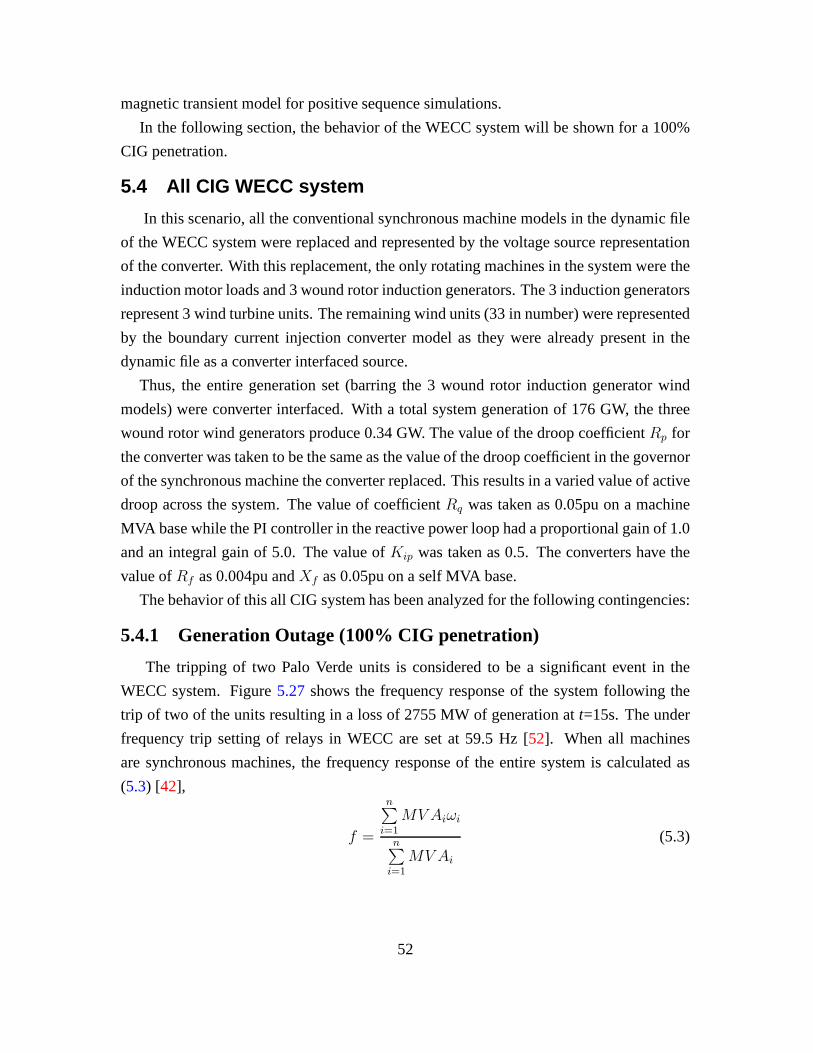
magnetic transient model for positive sequence simulations.
In the following section, the behavior of the WECC system will be shown for a 100%
CIG penetration.
5.4 All CIG WECC system
In this scenario, all the conventional synchronous machinemodels in the dynamic file
of the WECC system were replaced and represented by the voltage source representation
of the converter. With this replacement, the only rotating machines in the system were the
induction motor loads and 3 wound rotor induction generators. The 3 induction generators
represent 3 wind turbine units. The remaining wind units (33in number) were represented
by the boundary current injection converter model as they were already present in the
dynamic file as a converter interfaced source.
Thus, the entire generation set (barring the 3 wound rotor induction generator wind
models) were converter interfaced. With a total system generation of 176 GW, the three
wound rotor wind generators produce 0.34 GW. The value of thedroop coefficientRp for
the converter was taken to be the same as the value of the droopcoefficient in the governor
of the synchronous machine the converter replaced. This results in a varied value of active
droop across the system. The value of coefficientRq was taken as 0.05pu on a machine
MVA base while the PI controller in the reactive power loop had a proportional gain of 1.0
and an integral gain of 5.0. The value ofKip was taken as 0.5. The converters have the
value ofRf as 0.004pu andXf as 0.05pu on a self MVA base.
The behavior of this all CIG system has been analyzed for the following contingencies:
5.4.1 Generation Outage (100% CIG penetration)
The tripping of two Palo Verde units is considered to be a significant event in the
WECC system. Figure5.27 shows the frequency response of the system following the
trip of two of the units resulting in a loss of 2755 MW of generation at t=15s. The under
frequency trip setting of relays in WECC are set at 59.5 Hz [52]. When all machines
are synchronous machines, the frequency response of the entire system is calculated as
(5.3) [42],
f =
n∑
i=1
MVAiωi
n∑
i=1
MV Ai
(5.3)
52
5 10 15 20 25 30 35 4059.8
59.85
59.9
59.95
60
Time (s)
Fre
quen
cy (
Hz)
ArizonaSouthern CaliforniaPacific Gas and ElectricNorthwestB.C.Hydro 15 15.5 16 16.5 17 17.5 18
59.88
59.9
59.92
59.94
59.96
59.98
60
60.02
Time (s)
ArizonaSouthern CaliforniaPacific Gas and ElectricNorthwestB.C.Hydro
Figure 5.27: Frequency across five generation areas for the trip of two Palo Verde units (droop coefficientof each CIG unit isRp)
whereMV Ai is the rating of the machine,ωi is the speed of the machine andn is the
number of synchronous machines. However in a system where all sources are interfaced
through converters, the speed of rotation of a machine (if present) behind the converter
will not give any picture of the system frequency as it is electrically decoupled from the
network. Thus an approximate frequency has been obtained byperforming a numerical
differentiation of the bus voltage angle. The plots in Figure 5.27 show the calculated
frequency in the five major generating areas of the WECC system which account for 63.4%
of the total system generation while Figure5.28shows the actual active power in four of
these areas.
It can be seen that the largest excursion in frequency occursin the Arizona area as ex-
pected. Further, even with the total inertia of the system being close to zero, the frequency
nadir is well above the under frequency trip setting. The fast action of the converters and
their associated control help in arresting the rate of decrease of frequency and bring about
a steady state operation quickly. The frequency settles at 59.965 Hz. Due to the highly
meshed network, the bus voltage angles in different parts ofthe network change in varied
ways and this can also be observed from the frequency plot.
As the third unit at Palo Verde is the closest to the outage, the response of the converter
representing this unit can be informative. The active power, reactive power, terminal volt-
53

5 10 15 20 25 30 35 401.65
1.7
1.75x 10
4
Time (s)
Pow
er (
MW
)
5 10 15 20 25 30 35 402.85
2.9
2.95x 10
4
Time (s)
Pow
er (
MW
)
5 10 15 20 25 30 35 402.9
2.95x 10
4
Time (s)
Pow
er (
MW
)
5 10 15 20 25 30 35 401.1
1.12
1.14x 10
4
Time (s)
Pow
er (
MW
)
(b) Pacific Gas and Electric
(a) Southern California
(d) B. C. Hydro
(c) Northwest
Figure 5.28: Active power output in four areas of WECC following the trip of two Palo Verde units
age and current of the converter representing the third PaloVerde unit is as shown in
Figure5.29. It can be seen that the converter response is quick and none of the limits are
violated. The converter current is well within its maximum rating and the voltage control
loop maintains the voltage at the pre-fault value. As the Palo Verde units are operated
close to their maximum active power limit, there is very little reserve margin available.
To observe the effect of the active power droop coefficient, two further simulations were
run. In the first, the values of the droop coefficient were doubled while in the second they
were halved. Thus, if we denoteRp as the droop coefficient of each CIG unit for the plot
in Figure5.27, the values of the droop coefficients were made2Rp andRp/2 in order to
observe the effect of droop. Individual CIG units may still have different values of droop
as the coefficientRp takes on different values for each unit as mentioned at the start of
this section. The frequency plots of Figures.5.30and5.31show the performance for the
trip of two Palo Verde units when the values of the droop coefficient were2Rp andRp/2
respectively.
It can be observed that changing the value of the coefficient changes the final steady
state value of the frequency. When the coefficient value is increased, it signifies that the
same change in active power will cause a greater reduction infrequency while when the
coefficient value is decreased, the reduction in frequency is lower. In Figure5.30, the
frequency settles around 59.933 Hz while in Figure5.31, the frequency settles at 59.982
54

5 10 15 20 25 30 35 401200
1400
1600
1800
Pow
er (
MW
)
5 10 15 20 25 30 35 40300
350
400
Pow
er (
MV
AR
)
5 10 15 20 25 30 35 40
0.9951.0
1.01
1.02
Vol
tage
(pu
)
5 10 15 20 25 30 35 400.8
1
1.2
Time (s)
Cur
rent
(pu
)
(b) Reactive Power
(c) Terminal Voltage
(a) Active Power
(d) Converter Current
Figure 5.29: Behavior of the third Palo Verde unit for the trip of two other Palo Verde units
5 10 15 20 25 30 35 40 45 50 55 6059.88
59.9
59.92
59.94
59.96
59.98
60
60.02
60.04
60.06
60.08
Time (s)
Fre
quen
cy (
Hz)
ArizonaSouthern CaliforniaPacific Gas and ElectricNorthwestB.C.Hydro
15 15.5 16 16.5 17 17.5 1859.88
59.9
59.92
59.94
59.96
59.98
60
60.02
Time (s)
ArizonaSouthern CaliforniaPacific Gas and ElectricNorthwestB.C.Hydro
Figure 5.30: Frequency across five generation areas for the trip of two Palo Verde units (droop coefficientof each CIG unit is2Rp)
Hz. This is in comparison to the settling frequency of 59.965Hz in Figure5.27. The
frequency nadir changes slightly with change in the value ofthe droop coefficient. With
droop coefficientRp, the frequency nadir is 59.8973 Hz. With a droop value of2Rp, the
55

5 10 15 20 25 30 35 40
59.86
59.88
59.9
59.92
59.94
59.96
59.98
60
60.02
Time (s)
Fre
quen
cy (
Hz)
ArizonaSouthern CaliforniaPacific Gas and ElectricNorthwestB.C.Hydro 15 15.5 16 16.5 17 17.5 18
59.88
59.9
59.92
59.94
59.96
59.98
60
Time (s)
ArizonaSouthern CaliforniaPacific Gas and ElectricNorthwestB.C.Hydro
Figure 5.31: Frequency across five generation areas for the trip of two Palo Verde units (droop coefficientof each CIG unit isRp/2)
nadir is 59.896 Hz while with a droop value ofRp/2, the nadir is 59.902 Hz.
In addition, this comparison brings to light the fact that although CIG units are fast
acting, a finite time is required to bring about a steady stateoperation as rotating elements
are still present in the system in the form of induction motors. The inertia of these motors
play a role in the transient behavior of the system. There is also a difference in settling
time with different values of droop coefficients and this canbe seen from all frequency
plots.
In all subsequent scenarios, the value of the droop coefficient has been assumed to be
Rp.
In terms of computation time, with a droop coefficientRp, PSLF took 8:10 minutes to
run the 40 second simulation of this generation outage scenario with the first 20 seconds of
simulation taking 3:52 minutes. The simulation was run on a machine with an i7 processor
and 16.0 gb of RAM with a simulation time step of 0.0041s. It can be concluded that an
all CIG system is capable of providing a stable frequency response through the fast action
of the controllers and the simulation is numerically stabletoo.
56

5.4.2 Dc Voltage Dip and Subsequent Recovery (100% CIG penetra-
tion)
In all of the above scenarios, the dc voltage has been assumedto be constant, implying
a battery as a source of power. However, even for units of a size as low as 100 MVA, the
assumption of a battery as a constant source of power is not realistic. A practical source
can either be a gas or hydro turbine (synchronous machine) ora solar/wind farm. Such
sources would require a capacitor on the dc bus to maintain a constant voltage input to the
inverter. However, a disturbance in the network would causefluctuations in the current
levels causing the dc voltage across the capacitor and thus across the converter switches
to vary. It is hence important to study the effect of this variable dc voltage on the system
behavior.
At t=15s, two Palo Verde units are tripped resulting in a generation outage of 2755MW.
With a capacitor on the dc link, the immediate response to this contingency would be an
increase in the converter current and a decrease in capacitor voltage. Gradually as the
active power control reacts (with synchronous machine control being the slowest), the
capacitor voltage will be restored. To simulate this situation, the dc voltage on all CIG
units participating in frequency regulation was reduced by1%, 20ms after the generation
outage. Gradually, over the subsequent 10s, the dc voltage was restored. The frequency
plot for this scenario is as shown in Figure5.32while Figure5.33shows the active power,
reactive power, terminal voltage and current of the third Palo Verde unit.
The sudden reduction in generation att=15s causes the frequency to drop to 59.89 Hz
in the Arizona area. The subsequent reduction in dc voltage causes the terminal voltage
of CIG units to drop by a larger extent when compared to the terminal voltage drop for
just the trip of the units. This can be observed by comparing Figure5.33(c) with Figure
5.29(c). This drop in voltage results in a reduction of load (voltage dependent load) thereby
causing the frequency to rise. The voltage drop also resultsin the tripping of a motor due to
activation of the under voltage load shedding relay at the motor terminals. The subsequent
recovery of the dc voltage and its effect on the system is apparent from Figure5.33.
The results of this scenario are a set of conservative results as the dc voltage has been
assumed to drop only on those CIG units that take part in frequency regulation. In reality,
the voltage would drop at all units. However, the recovery ofthe voltage is possible only on
units that take part in frequency regulation. Further, for adc voltage drop greater than 1%,
multiple converters trip due to overcurrent and multiple motors trip due to under voltage.
In practice, the size of the capacitor at the dc bus would haveto be designed so as to
57

5 10 15 20 25 30 35 4059.85
59.9
59.95
60
60.05
60.1
60.15
60.2
Time (s)
Fre
quen
cy (
Hz)
ArizonaSouthern CaliforniaPacific Gas and ElectricNorthwestB.C.Hydro
15 15.5 16 16.5 17 17.5 18
59.9
59.95
60
60.05
60.1
60.15
60.2
Time (s)
ArizonaSouthern CaliforniaPacific Gas and ElectricNorthwestB.C.Hydro
Figure 5.32: Frequency across five generation areas for the trip of two Palo Verde units followed by thereduction in dc voltage by 1% and its subsequent recovery
5 10 15 20 25 30 35 401200
1400
1600
1800
Pow
er (
MW
)
5 10 15 20 25 30 35 40200
300
400
500
Pow
er (
MV
AR
)
5 10 15 20 25 30 35 400.85
0.9
0.95
1
1.05
Vol
tage
(pu
)
5 10 15 20 25 30 35 400.8
1
Time (s)
Cur
rent
(pu
)
(a) Active Power
(b) Reactive Power
(c) Terminal Voltage
(d) Converter Current
Figure 5.33: Behavior of the third Palo Verde unit for the trip of two other Palo Verde units followed by thereduction in dc voltage by 1% and its subsequent recovery
restrict the drop in voltage to less than 1%. Additionally, fast acting units may have to
be brought online to support the voltage and in order to maintain the system reliability, a
coordinated, well designed wide area control action may be required.
58
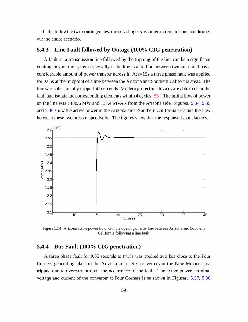
In the following two contingencies, the dc voltage is assumed to remain constant through-
out the entire scenario.
5.4.3 Line Fault followed by Outage (100% CIG penetration)
A fault on a transmission line followed by the tripping of theline can be a significant
contingency on the system especially if the line is a tie linebetween two areas and has a
considerable amount of power transfer across it. Att=15s a three phase fault was applied
for 0.05s at the midpoint of a line between the Arizona and Southern California areas. The
line was subsequently tripped at both ends. Modern protection devices are able to clear the
fault and isolate the corresponding elements within 4 cycles [53]. The initial flow of power
on the line was 1408.6 MW and 134.4 MVAR from the Arizona side.Figures.5.34, 5.35
and5.36show the active power in the Arizona area, Southern California area and the flow
between these two areas respectively. The figures show that the response is satisfactory.
5 10 15 20 25 30 35 402.1
2.15
2.2
2.25
2.3
2.35
2.4
2.45
2.5
2.55
2.6x 10
4
Time(s)
Pow
er (
MW
)
Figure 5.34: Arizona active power flow with the opening of a tie line between Arizona and SouthernCalifornia following a line fault
5.4.4 Bus Fault (100% CIG penetration)
A three phase fault for 0.05 seconds att=15s was applied at a bus close to the Four
Corners generating plant in the Arizona area. Six converters in the New Mexico area
tripped due to overcurrent upon the occurrence of the fault.The active power, terminal
voltage and current of the converter at Four Corners is as shown in Figures.5.37, 5.38
59
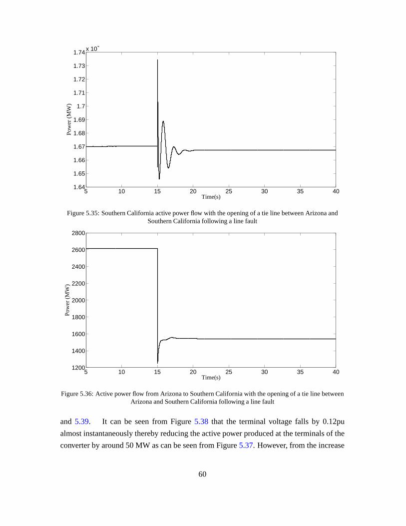
5 10 15 20 25 30 35 401.64
1.65
1.66
1.67
1.68
1.69
1.7
1.71
1.72
1.73
1.74x 10
4
Time(s)
Pow
er (
MW
)
Figure 5.35: Southern California active power flow with the opening of a tie line between Arizona andSouthern California following a line fault
5 10 15 20 25 30 35 401200
1400
1600
1800
2000
2200
2400
2600
2800
Time(s)
Pow
er (
MW
)
Figure 5.36: Active power flow from Arizona to Southern California with the opening of a tie line betweenArizona and Southern California following a line fault
and 5.39. It can be seen from Figure5.38 that the terminal voltage falls by 0.12pu
almost instantaneously thereby reducing the active power produced at the terminals of the
converter by around 50 MW as can be seen from Figure5.37. However, from the increase
60

5 10 15 20 25 30 35 40190
200
210
220
230
240
250
260
270
Time (s)
Pow
er (
MW
)
Figure 5.37: Active power of a Four Corner unit for a three phase bus fault near the unit
5 10 15 20 25 30 35 400.86
0.88
0.9
0.92
0.94
0.96
0.98
1
1.02
1.04
Time (s)
Vol
tage
(pu
)
Figure 5.38: Terminal voltage of a Four Corner unit for a three phase bus fault near the unit
in current in Figure5.39, it can be inferred that the reactive power produced increases to
bring the voltage level back to 1.0pu within 3 seconds. The absence of an oscillatory mode
for a fault close to a source is a significant observation thatcan be made from this scenario.
61

5 10 15 20 25 30 35 400.98
1
1.02
1.04
1.06
1.08
1.1
1.12
1.14
Time (s)
Cur
rent
(pu
)
Figure 5.39: Current of a Four Corner unit for a three phase bus fault near the unit
5.4.5 Line Reconnection (100% CIG penetration)
To observe the effect of a line re-closure over large terminal bus voltage angles, the line
between Moenkopi and Four Corners was initially outaged andthe power flow was solved.
This resulted in an angle difference of around 40 degrees between the buses. During the
simulation, att = 15s, the line was reclosed. The current of one of the Four Corners
units, located near the line is as shown in Figure5.40. It can be seen from the figure that
the current rises to 1.5pu at the instant of re-closure but regains its pre-disturbance value
within a second. The maximum value of current has been taken to be 1.7pu in this case.
The current of another Four Corners unit located one bus awayfrom this unit is as shown
in Figure5.41. It can be seen from the figures that the converters have no problem in
dealing with the line re-closure and the performance is satisfactory. In order to observe
the behavior with a lower current rating, the maximum current of the just the Four Corners
units were set as 1.4pu. With this setting, the simulation was run once again. This time,
due to the lower current setting and due to the overcurrent trip mechanism, the unit located
closer to the line tripped while the remaining units took up the surplus power. This can be
seen from the current of the Four Corners unit located one busaway as shown in Figure
5.42.
The total active power output from the Arizona area for both values of maximum cur-
rent is as shown in Figure5.43. From the figures, it can be seen that the system is capable
62

Time (s)5 10 15 20 25 30 35 40
Cur
rent
(pu
)
0.8
0.9
1
1.1
1.2
1.3
1.4
1.5
Figure 5.40: Current of a Four Corners unit for a line re-closure near the unit
Time (s)5 10 15 20 25 30 35 40
Cur
rent
(pu
)
0.85
0.9
0.95
1
1.05
1.1
Figure 5.41: Current of a Four Corners unit located one bus away
of withstanding the re-closure of a large line. The results of this section show that the
preliminary tests on the performance of an all CIG system arepositive.
The next section describes the performance of the inductionmotor drive model
63

Time (s)5 10 15 20 25 30 35 40
Cur
rent
(pu
)
0.85
0.9
0.95
1
1.05
1.1
1.15
1.2
1.25
Figure 5.42: Current of a Four Corners unit located one bus away for lower maximum current
Time (s)5 10 15 20 25 30 35 40
Pow
er (
MW
)
×104
2.44
2.46
2.48
2.5
2.52
2.54
2.56
2.58
Four Corners Imax - 1.7puFour Corners Imax - 1.4pu
Figure 5.43: Total Arizona active power for line re-closure
5.5 Induction Motor Drive Model
The validation of the motor speed drive model was carried outin an independently
developed, in-house C program capable of performing positive sequence time domain
simulations. The network of Figure5.6 was used as a test system and the static load at
64

0 1 2 3 4 5 6 7 8 9 100.9048
0.905
0.9052
0.9054
0.9056
0.9058
0.906
0.9062
Time (s)
Spe
ed (
pu)
With constant speed driveWithout constant speed drive
Figure 5.44: Speed of induction motor for both the presence and absence of a constant speed drive for a 10MW load increase
0 1 2 3 4 5 6 7 8 9 10−1.145
−1.14
−1.135
−1.13
−1.125
−1.12
−1.115
−1.11
Time (s)
Tor
que
(pu)
With constant speed driveWithout constant speed drive
0.8 0.85 0.9 0.95 1 1.05 1.1 1.15 1.2
−1.14
−1.135
−1.13
−1.125
−1.12
−1.115
Time (s)
With constant speed driveWithout constant speed drive
Figure 5.45: Load torque of induction motor for both the presence and absence of a constant speed drivefor a 10 MW load increase
bus 5 was replaced by an induction motor with an inertiaH=1.2s. In order to obtain the
value of slip and the reactive power consumed by the motor fora given active power load,
the procedure of incorporating the equations of the motor into the Newton Raphson power
flow algorithm as detailed in [54] was made use off.
For an active power load increase of 10 MW at bus 6 att=1s, Figure5.44shows the
65

0 1 2 3 4 5 6 7 8 9 10−125.5
−125
−124.5
−124
−123.5
−123
−122.5
−122
−121.5
Time (s)
Pow
er (
MW
)
With constant speed driveWithout constant speed drive
0.85 0.9 0.95 1 1.05 1.1 1.15 1.2
−125
−124.5
−124
−123.5
−123
−122.5
−122
Time (s)
With constant speed driveWithout constant speed drive
Figure 5.46: Active power consumed by induction motor for both the presence and absence of a constantspeed drive for a 10 MW load increase
0 1 2 3 4 5 6 7 8 9 10−43.7
−43.6
−43.5
−43.4
−43.3
−43.2
−43.1
−43
−42.9
−42.8
−42.7
Time (s)
Pow
er (
MV
AR
)
With constant speed driveWithout constant speed drive
Figure 5.47: Reactive power consumed by induction motor forboth the presence and absence of a constantspeed drive for a 10 MW load increase
speed of the induction motor for both the presence and absence of the constant speed drive.
The proportional and integral controller gains of the drivewere 5.0 and 4.0 respectively. It
can be seen that the positive sequence constant speed drive model is able to maintain the
speed of the motor at the pre-contingency value. The load torque on the motor is shown in
Figure5.45.
66

The negative value indicates that it is a load on the system. As the load on the induction
motor has not changed, the load torque is expected to remain the same and it can be seen
that is the case. However, due to the change in speed, the electrical power drawn by the
motor from the network would have changed to maintain the same level of torque. This
can be seen from Figures5.46and5.47wherein the active and reactive power consumed
by the motor is shown.
When a motor is enabled with a constant speed drive, the active power consumed re-
duces as the speed is maintained at a higher value when compared to the drop in speed
without a drive. A load increase in the system reduces the voltage magnitude at all un-
controlled buses in the system and this causes the speed of the motor to drop. However,
when the motor is enabled with a constant speed drive, the speed is maintained by ensur-
ing that the flux in the air gap remains constant. Thus, if the terminal voltage drops, then
the frequency of the inverter output is also reduced to maintain the value of flux thereby
maintaining the speed.
67

6. Conclusion and Future Research
The future grid will be served by sources of energy whose characteristics will be de-
coupled from the network due to the presence of an interface converter. For the scope of
this project, these sources are known as converter interfaced generation (CIG). With an
increasing penetration of such sources, the behavior of thebulk power system has been
analyzed. To do this, reliable models for the converter and its control were developed for
use in commercial grade software to showcase the complex interactions of these models
with one another.
The goals achieved by this research work are listed as below:
1. A reliable converter model based on the voltage source representation of the con-
verter was developed by using an electromagnetic transientlevel model of the con-
verter as a basis.
2. A straightforward control structure for the converter was developed.
3. The converter model and its associated control was incorporated into the commercial
software PSLF using ’user written models’ after being tested on an independently
developed, in-house C code capable of performing positive sequence time domain
simulations on small test systems.
4. The greater accuracy of the voltage source representation of the converter over the
boundary current injection representation was showcased.
5. The behavior of the large WECC system with all converter interfaced sources was
analyzed under various contingent situations and the behavior was found to be
largely satisfactory with the converters contributing to both frequency regulation
and reactive power support.
6. A positive sequence model for an induction motor speed control drive was developed
and its performance was observed in a small all CIG test system.
During the course of this research work, new questions were raised which can lead to
avenues for future research work such as:
1. When the dc voltage of the inverter dropped by more than 1% upon the occurrence
of a contingency, widespread tripping of induction motors due to undervoltage and
68

converters due to overcurrent occurred. It is possible thata well coordinated wide
area control strategy could increase the system reliability by bringing voltage sup-
port units online quickly.
2. As a planning problem, a capacitor of appropriate size will have to be placed on the
dc bus to reduce the voltage drop. Further, it is possible that different locations in
the system can withstand different amounts of drop in voltage on the dc bus. This
problem would have to be analyzed and addressed.
3. Until now, the source behind the inverter has not been modeled. However, it is
important to model these sources as the recovery of the dc side voltage depends on
the characteristics and control of the source. Developmentof a complete positive
sequence model of the source and its associated converter for use in commercial
time domain simulation software is the need of the hour.
4. For large systems, a robust analytical tuning procedure of the controller gains is
required. This would ensure the maximum utilization of the converter bandwidth
and bring about a healthy system operation.
5. Currently, the stress on the blades of a steam turbine determines the operating fre-
quency range of the system. With an all CIG system, an optimalfrequency range is
yet to be determined.
6. The behavior of induction motors and their associated drive mechanism has been
tested only on a small system. Their behavior and interaction with CIG in a large
system is yet to be seen.
69

References
[1] “Electricity in the United States,” U.S. Energy Information Administration, April 10,
2013, [Online]: http://www.eia.gov/energyexplained/index.cfm?page=electricity in
the unitedstates[Accessed: August 10, 2014].
[2] K. Clark, N. W. Miller, and R. Walling, “Modeling of GE solar photovoltaic plants
for grid studies,” GE Energy, Tech. Rep. 1.1, April 2010.
[3] N. W. Miller, W. W. Price, and J. J. Sanchez-Gasca, “Dynamic modeling of ge 1.5
and 3.6 wind turbine-generators,” GE Power Systems, Tech. Rep. 3.0, October 2003.
[4] PSLF User’s Manual, General Electric International, Inc., 2013.
[5] “Associated material for 2012 HS4A approved operating case,” Western Electricity
Coordinating Council, January 2012.
[6] I. Kolesnikov, “World reserves of fossil fuels,” 2013, [Online]: http://knoema.com/s
msfgud/world-reserves-of-fossil-fuels[Accessed: August 10, 2014].
[7] S. Shafiee and E. Topal, “When will fossil fuel reserves bediminished?” Energy
Policy, vol. 37, no. 1, pp. 181 – 189, 2009.
[8] A. Breidthardt, “German government want nuclear exit by2022 at latest,” Reuters,
May 30, 2011, [Online]:http://uk.reuters.com/article/2011/05/30/us-germany-nucle
ar-idUKTRE74Q2P120110530[Accessed: August 10, 2014].
[9] “Nuclear power: When the steam clears,” The Economist, March 24, 2011, [Online]:
http://www.economist.com/node/18441163[Accessed: August 10, 2014].
[10] J. Chandler, “Is this the end of the nuclear revival,” The Sydney Morning Her-
ald, March 19, 2011, [Online]:http://www.smh.com.au/environment/energy-smart/
is-this-the-end-of-the-nuclear-revival-20110318-1c0i9.html [Accessed: August 10,
2014].
[11] D. Gautam, V. Vittal, and T. Harbour, “Impact of increased penetration of dfig-based
wind turbine generators on transient and small signal stability of power systems,”
IEEE Trans. Power Syst., vol. 24, no. 3, pp. 1426–1434, Aug 2009.
70

[12] A. Azmy and I. Erlich, “Impact of distributed generation on the stability of electrical
power system,” in2005 IEEE Power Engineering Society General Meeting, June
2005, pp. 1056–1063.
[13] H. Storm, “Static magnetic exciter for synchronous alternators,”Transactions of the
American Institute of Electrical Engineers, vol. 70, no. 1, pp. 1014–1017, July 1951.
[14] L. M. Domeratzky, A. Rubenstein, and M. Temoshok, “A static excitation system
for industrial and utility steam turbine-generators,”Transactions of the American
Institute of Electrical Engineers Power Apparatus and Systems, Part III., vol. 80,
no. 3, pp. 1072–1077, April 1961.
[15] I. Report, “Proposed excitation system definitions forsynchronous machines,”IEEE
Trans. Power App. Syst., vol. PAS-88, no. 8, pp. 1248–1258, Aug 1969.
[16] P. Kundur, Power System Stability and Control, N. Balu and M. Lauby, Eds.
McGraw-Hill Education, 1994.
[17] S. Mishra, D. Ramasubramanian, and P. Sekhar, “A seamless control methodology
for a grid connected and isolated pv-diesel microgrid,”IEEE Trans. Power Syst.,
vol. 28, no. 4, pp. 4393–4404, Nov 2013.
[18] H. Bevrani, A. Ghosh, and G. Ledwich, “Renewable energysources and frequency
regulation: survey and new perspectives,”IET Renewable Power Generation, vol. 4,
no. 5, pp. 438–457, September 2010.
[19] R. de Almeida and J. Pecas Lopes, “Participation of doubly fed induction wind gen-
erators in system frequency regulation,”IEEE Trans. Power Syst., vol. 22, no. 3, pp.
944–950, Aug 2007.
[20] I. Erlich and M. Wilch, “Primary frequency control by wind turbines,” in2010 IEEE
Power and Energy Society General Meeting, July 2010, pp. 1–8.
[21] J. F. Conroy and R. Watson, “Frequency response capability of full converter wind
turbine generators in comparison to conventional generation,” IEEE Trans. Power
Syst., vol. 23, no. 2, pp. 649–656, May 2008.
[22] A. Attya and T. Hartkopf, “Control and quantification ofkinetic energy released by
wind farms during power system frequency drops,”IET Renewable Power Genera-
tion, vol. 7, no. 3, pp. 210–224, May 2013.
71

[23] T. Vandoorn, B. Meersman, J. De Kooning, and L. Vandevelde, “Transition from
islanded to grid-connected mode of microgrids with voltage-based droop control,”
IEEE Trans. Power Syst., vol. 28, no. 3, pp. 2545–2553, Aug 2013.
[24] K. Vidyanandan and N. Senroy, “Primary frequency regulation by deloaded wind
turbines using variable droop,”IEEE Trans. Power Syst., vol. 28, no. 2, pp. 837–846,
May 2013.
[25] R. Majumder, B. Chaudhuri, A. Ghosh, R. Majumder, G. Ledwich, and F. Zare, “Im-
provement of stability and load sharing in an autonomous microgrid using supple-
mentary droop control loop,”IEEE Trans. Power Syst., vol. 25, no. 2, pp. 796–808,
May 2010.
[26] Y. A. R. I. Mohamed and E. El-Saadany, “Adaptive decentralized droop controller
to preserve power sharing stability of paralleled inverters in distributed generation
microgrids,”IEEE Trans. Power Electron., vol. 23, no. 6, pp. 2806–2816, Nov 2008.
[27] E. Barklund, N. Pogaku, M. Prodanovic, C. Hernandez-Aramburo, and T. Green,
“Energy management in autonomous microgrid using stability-constrained droop
control of inverters,”IEEE Trans. Power Electron., vol. 23, no. 5, pp. 2346–2352,
Sept 2008.
[28] S. Ashabani and Y.-R. Mohamed, “General interface for power management of
micro-grids using nonlinear cooperative droop control,”IEEE Trans. Power Syst.,
vol. 28, no. 3, pp. 2929–2941, Aug 2013.
[29] G. Diaz, C. Gonzalez-Moran, J. Gomez-Aleixandre, and A. Diez, “Scheduling of
droop coefficients for frequency and voltage regulation in isolated microgrids,”IEEE
Trans. Power Syst., vol. 25, no. 1, pp. 489–496, Feb 2010.
[30] H. Xin, Y. Liu, Z. Wang, D. Gan, and T. Yang, “A new frequency regulation strat-
egy for photovoltaic systems without energy storage,”IEEE Trans. Sustain. Energy,
vol. 4, no. 4, pp. 985–993, Oct 2013.
[31] W. Omran, M. Kazerani, and M. Salama, “Investigation ofmethods for reduction of
power fluctuations generated from large grid-connected photovoltaic systems,”IEEE
Trans. Energy Convers., vol. 26, no. 1, pp. 318–327, March 2011.
72

[32] M. Datta, T. Senjyu, A. Yona, T. Funabashi, and C.-H. Kim, “A frequency-control
approach by photovoltaic generator in a pv-diesel hybrid power system,”IEEE Trans.
Energy Convers., vol. 26, no. 2, pp. 559–571, June 2011.
[33] N. Kakimoto, S. Takayama, H. Satoh, and K. Nakamura, “Power modulation of pho-
tovoltaic generator for frequency control of power system,” IEEE Trans. Energy Con-
vers., vol. 24, no. 4, pp. 943–949, Dec 2009.
[34] M. Morjaria and D. Anichkov, ““Grid Friendly” utility-scale PV plants,” White Pa-
per, First Solar, Aug 2013.
[35] M. A. Eltawil and Z. Zhao, “Grid-connected photovoltaic power systems: Techni-
cal and potential problemsa review,”Renewable and Sustainable Energy Reviews,
vol. 14, no. 1, pp. 112 – 129, January 2010.
[36] E. Vittal, M. O’Malley, and A. Keane, “Rotor angle stability with high penetrations
of wind generation,”IEEE Trans. Power Syst., vol. 27, no. 1, pp. 353–362, Feb 2012.
[37] J. Slootweg and W. Kling, “Impacts of distributed generation on power system tran-
sient stability,” in2002 IEEE Power Engineering Society Summer Meeting, vol. 2,
July 2002, pp. 862–867.
[38] R. Pearmine, Y. H. Song, and A. Chebbo, “Influence of windturbine behaviour on
the primary frequency control of the british transmission grid,” IET Renewable Power
Generation, vol. 1, no. 2, pp. 142–150, June 2007.
[39] D. Gautam, L. Goel, R. Ayyanar, V. Vittal, and T. Harbour, “Control strategy to
mitigate the impact of reduced inertia due to doubly fed induction generators on
large power systems,”IEEE Trans. Power Syst., vol. 26, no. 1, pp. 214–224, Feb
2011.
[40] S. Eftekharnejad, V. Vittal, G. Heydt, B. Keel, and J. Loehr, “Impact of increased
penetration of photovoltaic generation on power systems,”IEEE Trans. Power Syst.,
vol. 28, no. 2, pp. 893–901, May 2013.
[41] J. Quintero, V. Vittal, G. Heydt, and H. Zhang, “The impact of increased penetration
of converter control-based generators on power system modes of oscillation,”IEEE
Trans. Power Syst., vol. 29, no. 5, pp. 2248–2256, Sept 2014.
73

[42] N. W. Miller, M. Shao, S. Pajic, and R. D’Aquila, “Western wind and solar integra-
tion study phase 3 - frequency response and transient stability,” NREL, Tech. Rep.
NREL Report No. SR-5D00-62906, Dec 2014.
[43] N. Bottrell, M. Prodanovic, and T. Green, “Dynamic stability of a microgrid with
an active load,”IEEE Trans. Power Electron., vol. 28, no. 11, pp. 5107–5119, Nov
2013.
[44] P. Anderson and A. Fouad,Power system control and stability. IEEE Press, 2003.
[45] J. M. Undrill, “Structure in the computation of power-system nonlinear dynamical
response,”IEEE Trans. Power App. Syst., vol. PAS-88, no. 1, pp. 1–6, January 1969.
[46] K. Clark, R. Walling, and N. Miller, “Solar photovoltaic (pv) plant models in pslf,”
in 2011 IEEE Power and Energy Society General Meeting, July 2011, pp. 1–5.
[47] A. Ghoshal and V. John, “Anti-windup schemes for proportional integral and propor-
tional resonant controller,” inNational Power Electronic Conference, 2010.
[48] “PLECS,” Plexim Electrical Engineering Software,http://www.plexim.com/home.
[49] S. Yang, Q. Lei, F. Peng, and Z. Qian, “A robust control scheme for grid-connected
voltage-source inverters,”IEEE Trans. Ind. Electron., vol. 58, no. 1, pp. 202–212,
Jan 2011.
[50] “PSLF,” GE Energy Consulting,http://www.geenergyconsulting.com/practice-area/
software-products/pslf.
[51] B. K. Bose,Modern Power Electronics and AC Drives. Prentice Hall PTR, 2002.
[52] “Frequency response initiative report - the reliability role of frequency response,”
NERC, Tech. Rep., Oct 2012.
[53] M. Seelig, “Impact of new generator circuit-breaker technologies on power plant
availability and profitability,”Proceedings CEPSI, 2000.
[54] D. Ruiz-Vega, T. Asiain Olivares, and D. Olguin Salinas, “An approach to the initial-
ization of dynamic induction motor models,”IEEE Trans. Power Syst., vol. 17, no. 3,
pp. 747 – 751, Aug 2002.
74

Appendix A. EPCL Code for User Defined Converter Control
Model
/ * ************************************************** ************************************ * /
/ * ****** epcgen model f o r c o n v e r t e r a long w i th a s s o c i a t e d c o n t r o l********************** * /
/ * ************************************************** ************************************ * /
/ * Model comments and data d e s c r i p t i o n
Th is model d e p i c t s t h e c o n v e r t e r as a v o l t a g e sou rce and t h u shas x s r c as 0 . 05
Model I n p u t Parameters
r s r c 0 . 0
x s r c 0 . 05
Tr V o l tage t r a n s d u c e r t ime c o n s t a n t ( sec )
Kp P r o p o r t i o n a l Gain
Ki I n t e g r a l Gain
Kip I n t e g r a l Gain in a c t i v e power loop
K l i m i t Ant i−windup ga in
Rq Q−V droop c o e f f i c i e n t
TQ Q t ime de lay ( sec )
Rp P−f droop c o e f f i c i e n t
Tg Time c o n s t a n t ( sec )
T1 Lead t ime c o n s t a n t ( sec )
T2 Lag t ime c o n s t a n t ( sec )
TD P t ime de lay ( sec )
Ted Ed t ime de lay ( sec )
Teq Eq t ime de lay ( sec )
MWcap Maximum MW cap f o r t h e governor p a r t o f t h e c o n v e r t e r
Pmax Maximum A c t i v e power
Qmax Maximum R e a c t i v e Power
Qmin Minimum R e a c t i v e Power
dV V o l tage v a r i a t i o n f o r t r i p
d t Time f o r v o l t a g e v a r i a t i o n
Imax Max Cur ren t
T f l 1 . 0 − i n d i c a t e s t h a t governor i s a c t i v e
0 . 0 − i n d i c a t e s t h a t governor i s no t a c t i v e
Sample I n p u t dynamic data reco rd :
epcgen Busno . ”Bus Name” kV ” id ” : #9 mva =100.0 ” convepcv . p” 5 . 0 ” r s r c ” 0 .004 ” x s r c ” 0 . 05 ”Tr” 0 . 0 2 . . .
***** End o f comments* /
d e f i n e INIT 2
d e f i n e SORC 3
d e f i n e ALGE 4
d e f i n e RATE 5
75

d e f i n e OUTP 7
d e f i n e NETW 8
@mx = dypar [ 0 ] . cmi
@k = model [@mx] . k
@bus=model [@mx] . bus
@mode = dypar [ 0 ] . mode
@kgen = genbc [@k] . kgen
swi tch (@mode )
case SORC:
i f ( epcgen [@mx] . er>0.)
@delt = a r c t a n ( epcgen [@mx] . e i / epcgen [@mx] . e r )
e l s e i f ( epcgen [@mx] . er<0. and epcgen [@mx] . e i>=0.)
@delt = a r c t a n ( epcgen [@mx] . e i / epcgen [@mx] . e r )+ (1 . 570796327* 2 )
e l s e i f ( epcgen [@mx] . er<0. and epcgen [@mx] . e i<0.)
@delt = a r c t a n ( epcgen [@mx] . e i / epcgen [@mx] . e r )− (1.570796327* 2)
e l s e i f ( epcgen [@mx] . e r =0. and epcgen [@mx] . e i>0.)
@delt =1.570796327
e l s e i f ( epcgen [@mx] . e r =0. and epcgen [@mx] . e i<0.)
@delt =−1.570796327
e n d i f
/ * Using Vdc to g e t t h e r e q u i r e d v o l t a g e* /
@E = s q r t ( ( epcgen [@mx] . s6* epcgen [@mx] . s6 )+ ( epcgen [@mx] . s7* epcgen [@mx] . s7 ) )
@Vdc = epcgen [@mx] . v12
/ * d ropp ing Vdc 0 . 02 s a f t e r P a love rde t r i p
i f ( dypar [ 0 ] . t ime>=15.02 and dypar [ 0 ] . t ime<=25.02)
i f ( epcgen [@mx] . T f l =1 .0)
@drop =1.0 /100
@Vdc = ( ( dypar [ 0 ] . t ime−1 5 . 0 2 )* ( 1 / 1 0 . 0 )* @drop* epcgen [@mx] . v12 )+((1.0−@drop )* epcgen [@mx] . v12 )
e n d i f
e n d i f * /
@VT = epcgen [@mx] . v13
@wst = 2* (22 /7 )* 60* dypar [ 0 ] . t ime
@m = @E/@VT
i f (@m>1.0)
@m=1.0
/ * l og te rm (”Max modu la t i on index a t bus ” , busd [@bus ] . extnum,” <”) * /
e n d i f
i f (@m<0.4)
@m=0.4
/ * l og te rm (” Min modu la t i on index a t bus ” , busd [@bus ] . extnum,” <”) * /
e n d i f
i f ( epcgen [@mx] . s6>0.)
76

@delt1 = a r c t a n ( epcgen [@mx] . s7 / epcgen [@mx] . s6 )
e l s e i f ( epcgen [@mx] . s6<0. and epcgen [@mx] . s7>=0.)
@delt1 = a r c t a n ( epcgen [@mx] . s7 / epcgen [@mx] . s6 )+ (1 . 570796327* 2 )
e l s e i f ( epcgen [@mx] . s6<0. and epcgen [@mx] . s7<0.)
@delt1 = a r c t a n ( epcgen [@mx] . s7 / epcgen [@mx] . s6 )− (1.570796327* 2)
e l s e i f ( epcgen [@mx] . s6 =0. and epcgen [@mx] . s7>0.)
@delt1 =1.570796327
e l s e i f ( epcgen [@mx] . s6 =0. and epcgen [@mx] . s7<0.)
@delt1 =−1.570796327
e n d i f
@Va = 0 . 5*@m*@Vdc* cos ( ( @wst )+ @delt1 )
@Vb = 0 . 5*@m*@Vdc* cos ( ( @wst )+ @delt1−2.094395102)
@Vc = 0 . 5*@m*@Vdc* cos ( ( @wst )+ @delt1 +2.094395102)
@Ed = ( 2 / 3 )* ( (@Va* cos ( @wst ) ) + (@Vb* cos ( @wst−2.094395102) )+(@Vc* cos ( @wst +2 . 094395102) ) )
@Eq = (−2 /3 )* ( (@Va* s i n ( @wst ) ) + (@Vb* s i n ( @wst−2.094395102) )+(@Vc* s i n ( @wst +2 . 094395102) ) )
epcgen [@mx] . ang le = 1.570796327+ @delt
epcgen [@mx] . ed=@Ed
epcgen [@mx] . eq=@Eq
break
case NETW:
break
case ALGE:
break
case RATE:
@vmon = v o l t [ @bus ] . vm
@mvabase = gens [ @kgen ] . mbase
/ * S e t t i n g o f t h e l i m i t s * /
@x=epcgen [@mx] . Imax
@Qmax1=epcgen [@mx] . Qmax
@Qmax2= s q r t ( pow ( (@x* @mvabase ) , 2 ) / 1 . 1 9 0 4 7 ) / * 0 . 4 power f a c t o r * /
@deninv =2.0
i f (@vmon>0.8)
@qmax=@Qmax1−((@Qmax2−@Qmax1 )* (@vmon−1 . 0 )* 4 . 0 ) / * Qmax acco rd ing to v o l t a g e* /
e l s e
77

@qmax=@Qmax1−((@Qmax2−@Qmax1 )* ( 0 . 8−1 . 0 )* 4 . 0 ) / * Qmax acco rd ing to v o l t a g e* /
e n d i f
@qmin=epcgen [@mx] . Qmin
@lim=pow ( (@x* @mvabase ) ,2)−pow (@qmax, 2 )
i f ( @lim<0.0)
@qmax=0.9*@x* @mvabase
@lim=pow ( (@x* @mvabase) ,2)−pow (@qmax , 2 )
e n d i f
@pmax= s q r t ( @lim ) / * to p r e s e r v e t h e MVA* /
/ * V o l tage Transducer * /
epcgen [@mx] . ds1 = (@vmon−epcgen [@mx] . s1 ) / epcgen [@mx] . Tr
@verr = genbc [@k ] . v re f−epcgen [@mx] . s1−(epcgen [@mx] . Rq* gens [ @kgen ] . qgen / @mvabase )
/ * PI B lock * /
epcgen [@mx] . ds0 = epcgen [@mx] . Ki* ( @verr−(epcgen [@mx] . K l im i t* epcgen [@mx] . v3 ) )
@prop = epcgen [@mx] . Kp* @verr
@Qcmd = @prop+epcgen [@mx] . s0
@a=@Qcmd
i f ( (@Qcmd* @mvabase)>@qmax )
@Qcmd=@qmax / @mvabase
e n d i f
i f ( (@Qcmd* @mvabase)<@qmin )
@Qcmd=@qmin / @mvabase
e n d i f
epcgen [@mx] . v3=@a−@Qcmd
@Iqcmd =−@Qcmd/ epcgen [@mx] . s1
/ * Q t ime de lay * /
epcgen [@mx] . ds4 = ( @Iqcmd−epcgen [@mx] . s4 ) / epcgen [@mx] . TQ
/ * Governor t ime c o n s t a n t * /
@perr = genbc [@k ] . p re f−(netw [ @bus ] . f / ( 1 . 0* epcgen [@mx] . Rp ) )
epcgen [@mx] . ds2 = ( @perr−epcgen [@mx] . s2 ) / epcgen [@mx] . Tg
/ * Lead lag b lock * /
epcgen [@mx] . ds3 = ( epcgen [@mx] . s2−epcgen [@mx] . s3−(epcgen [@mx] . s2* epcgen [@mx] . T1 / epcgen [@mx] . T2 ) )
/ epcgen [@mx] . T2
@Pcmd = ( epcgen [@mx] . s3 +( epcgen [@mx] . s2* epcgen [@mx] . T1 / epcgen [@mx] . T2 ) )* epcgen [@mx] . MWcap/ @mvabase
78

i f ( ( @Pcmd* @mvabase)>@pmax )
@Pcmd=@pmax / @mvabase
e n d i f
i f ( epcgen [@mx] . T f l =0 . 0 )
@Pcmd=genbc [@k] . p r e f* epcgen [@mx] . MWcap/ @mvabase
e n d i f
@Ipcmd = (@Pcmd/ epcgen [@mx] . s1 )+ epcgen [@mx] . s8
/ * P t ime de lay * /
epcgen [@mx] . ds5 = ( @Ipcmd−epcgen [@mx] . s5 ) / epcgen [@mx] . TD
/ * C a l c u l a t i n g t h e i n n e r v o l t a g e * /
i f ( epcgen [@mx] . er>0.)
@delt = a r c t a n ( epcgen [@mx] . e i / epcgen [@mx] . e r )
e l s e i f ( epcgen [@mx] . er<0. and epcgen [@mx] . e i>=0.)
@delt = a r c t a n ( epcgen [@mx] . e i / epcgen [@mx] . e r )+ (1 . 570796327* 2 )
e l s e i f ( epcgen [@mx] . er<0. and epcgen [@mx] . e i<0.)
@delt = a r c t a n ( epcgen [@mx] . e i / epcgen [@mx] . e r )− (1.570796327* 2)
e l s e i f ( epcgen [@mx] . e r =0. and epcgen [@mx] . e i>0.)
@delt =1.570796327
e l s e i f ( epcgen [@mx] . e r =0. and epcgen [@mx] . e i<0.)
@delt =−1.570796327
e n d i f
@vq=(−epcgen [@mx] . e r* s i n ( @delt ) ) + ( epcgen [@mx] . e i* cos ( @delt ) )
@vd=( epcgen [@mx] . e r* cos ( @delt ) ) + ( epcgen [@mx] . e i* s i n ( @delt ) )
@iq=epcgen [@mx] . s4
@id=epcgen [@mx] . s5
@ed=@vd+(@id* epcgen [@mx] . r s r c )−(@iq* epcgen [@mx] . x s r c )
@eq=@vq+(@iq* epcgen [@mx] . r s r c )+ ( @id* epcgen [@mx] . x s r c )
epcgen [@mx] . ds6 = (@ed−epcgen [@mx] . s6 ) / epcgen [@mx] . Ted
epcgen [@mx] . ds7 = (@eq−epcgen [@mx] . s7 ) / epcgen [@mx] . Teq
epcgen [@mx] . ds8 = epcgen [@mx] . Kip* (@Pcmd−(gens [ @kgen ] . pgen / @mvabase ) )
/ * s e t v a r i a b l e s f o r o u t p u t f i l e * /
epcgen [@mx] . v0 = gens [ @kgen ] . pgen
epcgen [@mx] . v1 = gens [ @kgen ] . qgen
epcgen [@mx] . v2 = v o l t [ @bus ] . vm
/ * r ema in ing o u t p u t v a r i a b l e s* /
epcgen [@mx] . v4=@Qcmd* @mvabase
epcgen [@mx] . v5=@Pcmd* @mvabase
79

epcgen [@mx] . v6=@iq
epcgen [@mx] . v7=@id
epcgen [@mx] . v8= s q r t ( ( epcgen [@mx] . i t r* epcgen [@mx] . i t r )+ ( epcgen [@mx] . i t i* epcgen [@mx] . i t i ) )
epcgen [@mx] . v9= s q r t ( ( @id* @id )+ ( @iq* @iq ) )
/ * S e t t i n g t h e t r i p s e t t i n g s* /
/ * Overcu r ren t t r i p* /
i f ( dypar [ 0 ] . t ime>8.0)
i f ( epcgen [@mx] . v8> epcgen [@mx] . Imax )
gens [ @kgen ] . s t =0
epcgen [@mx] . v11= dypar [ 0 ] . t ime
log te rm ( ” T r i p p i n g c o n v e r t e r a t bus ” , busd [ @bus ] . extnum , ” due to o v e r c u r r e n t<” )
e n d i f
e n d i f
/ * Over v o l t a g e t r i p * /
i f ( dypar [ 0 ] . t ime>8.0)
i f ( ( @vmon−genbc [@k] . v r e f )>epcgen [@mx] . dV)
i f ( epcgen [@mx] . v10 =0 . 0 )
epcgen [@mx] . v10= dypar [ 0 ] . t ime
/ * l og te rm (” Over v o l t a g e t i m e r s t a r t e d a t bus ” , busd [@bus ] . extnum ,”<”) * /
e n d i f
i f ( ( dypar [ 0 ] . t ime−epcgen [@mx] . v10 )> epcgen [@mx] . d t )
gens [ @kgen ] . s t =0
log te rm ( ” T r i p p i n g c o n v e r t e r a t bus ” , busd [ @bus ] . extnum , ”due to o v e r v o l t a g e<” )
e n d i f
e n d i f
i f ( ( @vmon−genbc [@k] . v r e f )<epcgen [@mx] . dV and epcgen [@mx] . v10>0.0)
epcgen [@mx] . v10 =0.0
/ * l og te rm (” Over v o l t a g e t i m e r r e s e t a t bus ” , busd [@bus ] . extnum ,”<”) * /
e n d i f
e n d i f
break
case INIT :
@mvabase = gens [ @kgen ] . mbase
@pgen = gens [ @kgen ] . pgen / @mvabase
@qgen = gens [ @kgen ] . qgen / @mvabase
epcgen [@mx] . s1 = v o l t [ @bus ] . vm
genbc [@k] . v r e f = epcgen [@mx] . s1 +( epcgen [@mx] . Rq* @qgen )
epcgen [@mx] . s0 = @qgen
@iqcmd =−@qgen / epcgen [@mx] . s1
epcgen [@mx] . s4 = @iqcmd
epcgen [@mx] . v3 =0.0
80

genbc [@k] . p r e f = @pgen* @mvabase / epcgen [@mx] . MWcap
epcgen [@mx] . s2 = @pgen* @mvabase / epcgen [@mx] . MWcap
epcgen [@mx] . s3 = epcgen [@mx] . s2* (1−( epcgen [@mx] . T1 / epcgen [@mx] . T2 ) )
@pcmd = @pgen
@ipcmd = @pcmd / epcgen [@mx] . s1
epcgen [@mx] . s5 = @ipcmd
/ * C a l c u l a t i n g t h e i n n e r v o l t a g e * /
i f ( epcgen [@mx] . er>0.)
@delt = a r c t a n ( epcgen [@mx] . e i / epcgen [@mx] . e r )
e l s e i f ( epcgen [@mx] . er<0. and epcgen [@mx] . e i>=0.)
@delt = a r c t a n ( epcgen [@mx] . e i / epcgen [@mx] . e r )+ (1 . 570796327* 2 )
e l s e i f ( epcgen [@mx] . er<0. and epcgen [@mx] . e i<0.)
@delt = a r c t a n ( epcgen [@mx] . e i / epcgen [@mx] . e r )− (1.570796327* 2)
e l s e i f ( epcgen [@mx] . e r =0. and epcgen [@mx] . e i>0.)
@delt =1.570796327
e l s e i f ( epcgen [@mx] . e r =0. and epcgen [@mx] . e i<0.)
@delt =−1.570796327
e n d i f
@vq=(−epcgen [@mx] . e r* s i n ( @delt ) ) + ( epcgen [@mx] . e i* cos ( @delt ) )
@vd=( epcgen [@mx] . e r* cos ( @delt ) ) + ( epcgen [@mx] . e i* s i n ( @delt ) )
@iq=epcgen [@mx] . s4
@id=epcgen [@mx] . s5
@ed=@vd+(@id* epcgen [@mx] . r s r c )−(@iq* epcgen [@mx] . x s r c )
@eq=@vq+(@iq* epcgen [@mx] . r s r c )+ ( @id* epcgen [@mx] . x s r c )
epcgen [@mx] . s6 = @ed
epcgen [@mx] . s7 = @eq
epcgen [@mx] . s8 = 0 . 0
/ * o b t a i n i n g t h e va lue o f dc l i n k v o l t a g e* /
@E = s q r t ( ( @ed*@ed)+( @eq* @eq ) )
@VT = @E/ 0 . 6
@Vdc = @E/ ( 0 . 5* 0 . 6 )
epcgen [@mx] . v4=@qgen
i f ( epcgen [@mx] . T f l =0 . 0 )
epcgen [@mx] . v5=@pgen
e l s e
epcgen [@mx] . v5=@pgen
e n d i f
epcgen [@mx] . v6=@iq
epcgen [@mx] . v7=@id
epcgen [@mx] . v8= s q r t ( ( epcgen [@mx] . i t r* epcgen [@mx] . i t r )+ ( epcgen [@mx] . i t i* epcgen [@mx] . i t i ) )
epcgen [@mx] . v9= s q r t ( ( @id* @id )+ ( @iq* @iq ) )
epcgen [@mx] . v10 =0.0
81

epcgen [@mx] . v11 =0.0
epcgen [@mx] . v12=@Vdc
epcgen [@mx] . v13=@VT
epcgen [@mx] . ds0 = 0 . 0
epcgen [@mx] . ds1 = 0 . 0
epcgen [@mx] . ds2 = 0 . 0
epcgen [@mx] . ds3 = 0 . 0
epcgen [@mx] . ds4 = 0 . 0
epcgen [@mx] . ds5 = 0 . 0
epcgen [@mx] . ds6 = 0 . 0
epcgen [@mx] . ds7 = 0 . 0
epcgen [@mx] . ds8 = 0 . 0
epcgen [@mx] . ds9 = 0 . 0
channe l head [ 0 ] . t ype = ” pg ”
channe l head [ 0 ] . cmin = 0 .
channe l head [ 0 ] . cmax = 150.0
channe l head [ 1 ] . t ype = ” qg ”
channe l head [ 1 ] . cmin = −50.0
channe l head [ 1 ] . cmax = 50 . 0
channe l head [ 2 ] . t ype = ” v t ”
channe l head [ 2 ] . cmin = 0 .
channe l head [ 2 ] . cmax = 1.050
channe l head [ 3 ] . t ype = ” qwindup ”
channe l head [ 3 ] . cmin = 0 .
channe l head [ 3 ] . cmax = 1.050
channe l head [ 4 ] . t ype = ”qcmd”
channe l head [ 4 ] . cmin = 0 .
channe l head [ 4 ] . cmax = 1.050
channe l head [ 5 ] . t ype = ”pcmd”
channe l head [ 5 ] . cmin = 0 .
channe l head [ 5 ] . cmax = 1.050
channe l head [ 6 ] . t ype = ” iqcmd ”
channe l head [ 6 ] . cmin = 0 .
channe l head [ 6 ] . cmax = 1.050
channe l head [ 7 ] . t ype = ” ipcmd ”
channe l head [ 7 ] . cmin = 0 .
channe l head [ 7 ] . cmax = 1.050
channe l head [ 8 ] . t ype = ” I c u r r ”
channe l head [ 8 ] . cmin = 0 .
channe l head [ 8 ] . cmax = 1.050
channe l head [ 9 ] . t ype = ” Icmd”
channe l head [ 9 ] . cmin = 0 .
channe l head [ 9 ] . cmax = 1.050
break
case OUTP:
break
endcase
end
82

Appendix B. Three Generator Equivalent System Data
B.1 Power flow solution
The power flow solution along with the power demand and generation at each bus is as
tabulated in TableB.1.
Table B.1: Power Flow Solution for the three generator equivalent system
Bus Number V(pu) Ang(deg) Pd(MW) Qd(MVAR) Pg(MW) Qg(MVAR)
1 1.040 0.0 0.0 0.0 71.6 27.02 1.025 9.3 0.0 0.0 163.0 6.73 1.025 4.7 0.0 0.0 85.0 -10.94 1.026 -2.2 0.0 0.0 0.0 0.05 0.996 -4.0 125.0 50.0 0.0 0.06 1.013 -3.7 90.0 30.0 0.0 0.07 1.026 3.7 0.0 0.0 0.0 0.08 1.016 0.7 100.0 35.0 0.0 0.09 1.032 2.0 0.0 0.0 0.0 0.0
B.2 Dynamic data
The generator, exciter and governor data is as given as in Table B.2, B.3 andB.4 respec-
tively. The reactances in the generator data are given inpu on a 100 MVA base while the
time constants and the inertia constant are in seconds. The machine at bus 1 was modeled
using the GENSAL model while the other two machines were modeled using the GEN-
ROU models. A static exciter EXST1 was used on all machines while the governor model
Table B.2: Generator dynamic data for the three generator equivalent system
Bus Number MVA kV xd x′
d xq x′
q xℓ τ ′d0 τ ′q0 H
1 247.5 16.5 0.1460 0.0608 0.0969 0.0969 0.0336 8.96 0 23.642 192.0 18.0 0.8958 0.1198 0.8645 0.1969 0.0521 6.00 0.535 6.43 128.0 13.8 1.3125 0.1813 1.2578 0.25 0.0742 5.89 0.6 3.01
TGOV1 was used as a governor on all machines.
Table B.3: Exciter dynamic data for the three generator equivalent system
Bus Number Tr Vimax Vimin Tc Tb Ka Ta Vrmax Vrmin Kc Kf Tf Tc1 Tb1 Vamax Vamin Xe Ilr Klr
1 0.0 0.1 -0.1 1.0 10.0 200.0 0.02 5.0 -5.0 0.05 0.0 1.0 1.0 1.0 5.0 -5.0 0.04 2.8 5.02 0.0 0.1 -0.1 1.0 10.0 200.0 0.02 5.0 -5.0 0.05 0.0 1.0 1.0 1.0 5.0 -5.0 0.04 2.8 5.03 0.0 0.1 -0.1 1.0 10.0 200.0 0.02 5.0 -5.0 0.05 0.0 1.0 1.0 1.0 5.0 -5.0 0.04 2.8 5.0
83

Table B.4: Governor dynamic data for the three generator equivalent system
Bus Number MWcap R T1 Vmax Vmin T2 T3 Dt
1 247.5 0.05 0.5 1.0 0.01 1.0 10.0 0.02 192.0 0.05 0.5 1.0 0.01 1.0 10.0 0.03 128.0 0.05 0.5 1.0 0.01 1.0 10.0 0.0
84
Related Documents


