Stability of networked control systems

84 IEEE Control Systems Magazine February 2001

Feedback control systemswherein the control loops areclosed through a real-timenetwork are called net-worked control systems(NCSs) [1]-[4]. The defining

feature of an NCS is that information(reference input, plant output, controlinput, etc.) is exchanged using a net-work among control system compo-nents (sensors, controller, actuators,etc.). Fig. 1 illustrates a typical setupand the information flows of an NCS.The primary advantages of an NCS arereduced system wiring, ease of systemdiagnosis and maintenance, and in-creased system agility.

The insertion of the communication network in the feed-back control loop makes the analysis and design of an NCScomplex. Conventional control theories with many ideal as-sumptions, such as synchronized control and nondelayedsensing and actuation, must be reevaluated before they canbe applied to NCSs. Specifically, the following issues need tobe addressed. The first issue is the network-induced delay(sensor-to-controller delay and controller-to-actuator de-

lay) that occurs while exchanging data among devices con-nected to the shared medium. This delay, either constant(up to jitter) or time varying, can degrade the performanceof control systems designed without considering the delayand can even destabilize the system. Next, the network canbe viewed as a web of unreliable transmission paths. Somepackets not only suffer transmission delay but, even worse,can be lost during transmission. Thus, how such packet

Stability ofNetworked

Control Systems

Stability ofNetworked

Control Systems

By Wei Zhang, Michael S. Branicky, and Stephen M. Phillips

Zhang, Branicky ([email protected]), and Phillips are with the Electrical Engineering and Computer Science Department, Case WesternReserve University, 10900 Euclid Ave., Cleveland, OH 44106-7221, U.S.A.

0272-1708/01/$10.00©2001IEEE

©20

00Im

age

100

Ltd.

dropouts affect the performance of an NCS is an issuethat must be considered. Another issue is that plantoutputs may be transmitted using multiple networkpackets (so-called multiple-packet transmission), due tothe bandwidth and packet size constraints of the net-work. Because of the arbitration of the network me-dium with other nodes on the network, chances arethat all/part/none of the packets could arrive by thetime of control calculation.

The implementation of distributed control can betraced back at least to the early 1970s whenHoneywell’s Distributed Control System (DCS) was in-troduced. Control modules in a DCS are loosely con-nected because most of the real-time control tasks (sensing,calculation, and actuation) are carried out within individualmodules. Only on/off signals, monitoring information, alarminformation, and the like are transmitted on the serial net-work. Today, with help from ASIC chip design and significantprice drops in silicon, sensors and actuators can beequipped with a network interface and thus can become in-dependent nodes on a real-time control network. Hence, inNCSs, real-time sensing and control data are transmitted onthe network, and network nodes need to work closely to-gether to perform control tasks.

Current candidate networks for NCS implementationsare DeviceNet [5], Ethernet [6], and FireWire [7], to name afew. Each network has its own protocols that are designedfor a specific range of applications. Also, the behavior of anNCS largely depends on the performance parameters of theunderlying network, which include transmission rate, me-dium access protocol, packet length, and so on.

There are two main approaches for accommodating all ofthese issues in NCS design. One way is to design the controlsystem without regard to the packet delay and loss but designa communication protocol that minimizes the likelihood ofthese events. For example, various congestion control andavoidance algorithms have been proposed [8], [9] to gainbetter performance when the network traffic is above the limitthat the network can handle. The other approach is to treat thenetwork protocol and traffic as given conditions and designcontrol strategies that explicitly take the above-mentioned is-sues into account. To handle delay, one might formulate con-trol strategies based on the study of delay-differentialequations [10]. Here, we discuss analysis and design strate-gies for both network-induced delay and packet loss.

This article is organized as follows. First, we review someprevious work on NCSs and offer some improvements.Then, we summarize the fundamental issues in NCSs and ex-amine them with different underlying network-schedulingprotocols. We present NCS models with network-induceddelay and analyze their stability using stability regions and ahybrid systems technique. Following that, we discuss meth-ods to compensate network-induced delay and present ex-perimental results over a physical network. Then, we modelNCSs with packet dropout and multiple-packet transmis-

sion as asynchronous dynamical systems (ADSs) [11] andanalyze their stability. Finally, we present our conclusions.

Review of Previous WorkHalevi and Ray [1] consider a continuous-time plant and dis-crete-time controller and analyze the integrated communica-tion and control system (ICCS) using a discrete-timeapproach. They study a clock-driven controller with mis-syn-chronization between plant and controller. The system is rep-resented by an augmented state vector that consists of pastvalues of the plant input and output, in addition to the cur-rent state vectors of the plant and controller. This results in afinite-dimensional, time-varying discrete-time model. Theyalso take message rejection and vacant sampling into account.

Nilsson [2] also analyzes NCSs in the discrete-time do-main. He further models the network delays as constant, in-dependently random, and random but governed by anunderlying Markov chain. From there, he solves the LQG op-timal control problem for the various delay models. He alsopoints out the importance of time-stamping messages,which allows the history of the system to be known.

In Walsh et al. [3], the authors consider a continuousplant and a continuous controller. The control network,shared by other nodes, is only inserted between the sensornodes and the controller. They introduce the notion of maxi-mum allowable transfer interval (MATI), denoted by τ,which supposes that successive sensor messages are sepa-rated by at most τ seconds. Their goal is to find that value ofτ for which the desired performance (e.g., stability) of anNCS is guaranteed to be preserved.

It is assumed that the nonnetworked feedback system

[ ]( ) ( ), ( ) ( ), ( )x t A x t x t x t x tp c

T= =11

(where xp and xc represent the plant and controller state) isglobally exponentially stable. Thus, there exists a P such that

A P PA IT11 11+ = − . (1)

Next, it is assumed that the network’s effects can be com-puted by the error, e(t), between the plant output and con-troller input. So the networked system’s state vector is

February 2001 IEEE Control Systems Magazine 85

... Sensor n

ProcessesOtherControl Network

ProcessesOther

Controller

Actuator mActuator 1

Physical Plant

Sensor 1 ...

Figure 1. A typical NCS setup and information flows.

z t x t e tT T T( ) [ ( ), ( )]= , and thus the networked closed-loopsystem is

( ) ( )z t Az t=

where A can be partitioned as

AA A

A A=

11 12

21 22

.(2)

Walsh et al. study two scheduling methods: try-once-discard (TOD) and token-ring-type static scheduling. As-suming there are p sensor nodes connected to the NCS,static scheduling simply means that each node transmitsexactly once every p transmissions in a fixed order. Underthe MATI constraint, the controller must receive a transmis-sion from at least one of the sensors every τ seconds. Hence,under static scheduling, all sensor values are updated in atmost pτ seconds.

TOD is a scheduling protocol in which the node with the

greatest weighted error from its last reported value (to thecontroller) transmits its message. Again, the MATI con-straint ensures at least one such transmission every τ sec-onds. However, TOD does not guarantee that each node willtransmit once every p transmissions.

For each of these protocols, one can compute an upperbound on the MATI τ that preserves stability of theclosed-loop system. The result is given in the followingtheorem.

Theorem 1 [3, Theorem 2]: Given an NCS with p sensornodes operating under TOD or static scheduling, defineλ λ λ λ1 2= =min max( ), ( )P P (where P was defined above). If theMATI satisfies

τλ λ

λ λ λ

<+

=∑min

ln( ),

( / ),

/ (

2 1

8 1

1

16

2 1 1

2 2 12

p A A i

A

i

p

λ λ2 1 11/ )

,+

=∑ ii

p

then the NCS is globally exponentially stable.The calculation of the bound for τ can be generalized and

tightened by the following corollary.

Corollary 2: If the Lyapunov functionV x x PxT( ) = of the

nonnetworked, closed-loop system satisfies

A P PA QT11 11+ = − , (3)

(more general than (1)), where P Q, are positive-definitesymmetric matrices, the bound on τ becomes

τλ λ

λλ λ

<+

=∑min

ln( ),

( / ),

( )

2 1

8 1

16

2 1 1

2 2

p A A i

Q

i

p

min

/ ( / ).

λ λ λ12

2 1 11A i

i

p+

=∑

Furthermore, the third term is always the smallest, so

τ λλ λ λ λ λ

<+

=∑min( )

/ ( / )

Q

A ii

p16 12 2 1

22 1 1 (4)

guarantees the global exponential stability ofthe NCS.

Proof: See the Appendix.Corollary 2 shows that the MATI τ depends

on A p, , and Q; Q in turn determines P using(3). A and p are fixed for a particular systemsetup; thus Q is the only variable in choosing τ.One might use an analytic method to find the Qthat could maximize τ. By maximization wemean the largest τ possible that could still pre-serve stability of the NCS. However, the follow-

ing example illustrates the use of random search inchoosing τ.

Example 1: Consider the state-space plant model

. .,

x

x

x

xu

y

1

2

1

2

0 1

0 01

0

01

=

−

+

=

[ ] .1 0 1

2

x

x (5)

A continuous-state feedback controller is u Kx= − , whereK = [ . , . ]3 75 115 (closed-loop poles at –1/2 and –3/4).

Using Theorem 1, for p =1 (only one node, whichis a nonnetworked sampled-data system), we obtainτ = × −2 7 10 4. s. By randomly selecting Q and solving for P, wecan calculate τ using the formula in Corollary 2. In 200 trials,the maximum τ found was 4 5 10 4. × − s. However, the maxi-mum stable constant sampling period for this feedback con-trol system is 1.7 s (this can be determined using the“stability region” technique we discuss below), whichshows that Theorem 1 and Corollary 2 may be conservative.

Theorem 1 and Corollary 2 give sufficient conditions onthe network sampling rate to guarantee that the originalnonnetworked system remains stable when the control loopis closed over the network. They might be too conservative,

86 IEEE Control Systems Magazine February 2001

The defining feature of an NCS isthat information is exchanged usinga network among control systemcomponents.

however, to be of practical use. We later examine stabilityfor some specific examples to develop some insight into theproblem.

Fundamental Issues in NCSsIn this section, we will analyze some basic problems inNCSs, including network-induced delay, single-packet ormultiple-packet transmission of plant inputs and outputs,and dropping of network packets.

Network-Induced DelayThe network-induced delay in NCSs occurs when sensors,actuators, and controllers exchange data across the net-work. This delay can degrade the performance of controlsystems designed without considering it and can evendestabilize the system.

Depending on the medium access control (MAC) proto-col of the control network, network-induced delay can beconstant, time varying, or even random. MAC protocols gen-erally fall into two categories: random access and scheduling[12]. Carrier sense multiple access (CSMA) is most oftenused in random access networks, whereas token passing(TP) and time division multiple access (TDMA) are com-monly employed in scheduling networks.

Control networks using CSMA protocols includeDeviceNet [5] and Ethernet [6]. Fig. 2 illustrates various pos-sible situations for this type of network. The figure depictstwo nodes continually transmitting messages (with respectto a fixed time line). A node on a CSMA network monitors thenetwork before each transmission. When the network is idle,it begins transmission immediately, as shown in Case 1 of Fig.2. Otherwise it waits until the network is not busy. When twoor more nodes try to transmit simultaneously, a collision oc-curs. The way to resolve the collision is protocol dependent.DeviceNet, which is a controller area network (CAN), usesCSMA with a bitwise arbitration (CSMA/BA) protocol. SinceCAN messages are prioritized, the message with the highestpriority is transmitted without interruption when a collision

occurs, and transmission of the lower priority messageis terminated and will be retried when the network isidle, as shown in Case 2 of Fig. 2. Ethernet employs aCSMA with collision detection (CSMA/CD) protocol.When there is a collision, all of the affected nodes willback off, wait a random time (usually decided by the bi-nary exponential backoff algorithm [6]), and retransmit,as shown in Case 3 of Fig. 2. Packets on these types ofnetworks are affected by random delays, and theworst-case transmission time of packets is unbounded.Therefore, CSMA networks are generally considerednondeterministic. However, if network messages areprioritized, higher priority messages have a betterchance of timely transmission.

The TP protocol appears in token bus (IEEE Stan-dard 802.4), token ring (IEEE Standard 802.5) [6], andthe fiber distributed data interface (FDDI) MAC [13] ar-

chitectures; TDMA is used in FireWire [7]. A timing diagramfor this type of network is shown in Fig. 3. These protocolseliminate the contention for the shared network medium byallowing each node on the network to transmit according toa predetermined schedule. In a token bus, the token ispassed around a logical ring, whereas in a token ring, it ispassed around a physical ring. In scheduling networks, it ispossible to arrange for periodic transmission of messages.For example, FireWire has a transmission cycle (125 µs) di-vided into small time slots, where each isochronous trans-action is guaranteed a time slot to transmit in every cycle.Packet transmission delays on scheduling networks occurwhile waiting for the token or time slot. They can be madeboth bounded and constant by transmitting packets peri-odically.

Single-Packet versusMultiple-Packet TransmissionSingle-packet transmission means that sensor or actuatordata are lumped together into one network packet andtransmitted at the same time, whereas in multiple-packettransmission, sensor or actuator data are transmitted inseparate network packets, and they may not arrive at thecontroller and plant simultaneously. One reason for multi-ple-packet transmission is that packet-switched networkscan only carry limited information in a single packet due topacket size constraints. Thus, large amounts of data mustbe broken into multiple packets to be transmitted. The

February 2001 IEEE Control Systems Magazine 87

Case 2:When a collison occurson DeviceNet, one withhigher priority transmits

( +1)k h

( +1)k h ( +2)k h

( +2)k h

Case 3:When a collison occurson Ethernet, both backoff and transmit again

Node i

Node j

occursNo collisionCase 1:

kh

kh

Figure 2. Timing diagram for two nodes on a random access network.

Waiting for Tokenor Time Slot

Signal Ready

( +1)k h ( +2)k h

Signal Sent

kh

Node i

Figure 3. Timing diagram for an arbitrary node on a schedulingnetwork.

other reason is that sensors and actuators in an NCS are of-ten distributed over a large physical area, and it is impossi-ble to put the data into one network packet.

Conventional sampled-data systems assume that plantoutputs and control inputs are delivered at the same time,which may not be true for NCSs with multiple-packet trans-missions. Due to network access delays, the controller maynot be able to receive all of the plant output updates at thetime of the control calculation.

Different networks are suitable for different types oftransmissions. Ethernet, originally designed for transmit-ting information such as data files, can hold a maximum of1500 bytes of data in a single packet [6]. Hence, it is more ef-ficient to lump the sensor data into one packet and transmitit together—single-packet transmission. On the other hand,DeviceNet, featuring frequent transmission of small-sizecontrol data, has a maximum 8-byte data field in eachpacket; thus, sensor data often must be shuttled in differentpackets on DeviceNet.

Dropping Network PacketsNetwork packet drops occasionally happen on an NCS whenthere are node failures or message collisions. Althoughmost network protocols are equipped with transmis-sion-retry mechanisms, they can only retransmit for a lim-ited time. After this time has expired, the packets aredropped. Furthermore, for real-time feedback control datasuch as sensor measurements and calculated control sig-nals, it may be advantageous to discard the old,untransmitted message and transmit a new packet if it be-comes available. In this way, the controller always receivesfresh data for control calculation.

Normally, feedback-controlled plants can tolerate a cer-tain amount of data loss, but it is valuable to determinewhether the system is stable when only transmitting thepackets at a certain rate and to compute acceptable lowerbounds on the packet transmission rate.

Stability of NCSs withNetwork-Induced Delay

Modeling NCSs withNetwork-Induced DelayThe NCS model considering network-induced delay isshown in Fig. 4. The model consists of a continuous plant

( ) ( ) ( )

( ) ( )

x t Ax t Bu t

y t Cx t

= += (6)

and a discrete controller

u kh Kx kh k( ) ( ), , , ,= − =0 1 2 . (7)

Here, x n∈ R , u m∈ R , y p∈ R , and A B C K, , , are of compatibledimensions.

There are two sources of delays from the network: sen-sor-to-controller τ sc and controller-to-actuator τ ca . Any con-troller computational delay can be absorbed into either τ sc

or τ ca without loss of generality [2]. For fixed control law(time-invariant controllers), the sensor-to-controller delayand controller-to-actuator delay can be lumped together asτ τ τ= +sc ca for analysis purposes.

We consider the setup with a) clock-driven sensors thatsample the plant outputs periodically at sampling instants;b) an event-driven controller, which can be implemented byan external event interrupt mechanism and which calcu-lates the control signal as soon as the sensor data arrives;and c) event-driven actuators, which means the plant inputsare changed as soon as the data become available. The tim-ing of signals of the setup with τ < h is shown in Fig. 5.

Delay Less than One Sampling PeriodFirst consider the case where the delay of each sample, τ k , isless than one sampling period, h. (Here the subscript repre-sents the sampling instant.) This constraint means that at

88 IEEE Control Systems Magazine February 2001

ControlNetwork

τca

ControlNetwork

τsc

ContinuousTime Plant

Discrete TimeController

ZOHActuator Sensor

Continuous Signal

Digital Signal

h

Figure 4. NCS model with network-induced delay.

τk

τca,k

τsc,k u(kh)

u(kh)

( +2)k h

kh

( +2)k h

kh ( +1)k h

( +1)k h ( +2)k h

( +1)k h

Controller

Plant

Actuator

kh

x kh y kh( ) or ( )

Figure 5. Network-induced delay.

most two control samples,u k h(( ) )−1 andu kh( ), need be ap-plied during the kth sampling period. The system equationscan be written as

( ) ( ) ( ), [ , ( ) ),

( ) ( )

x t Ax t Bu t t kh k h

y t Cx tk k= + ∈ + + +

=+τ τ1 1

,

( ) ( ), , , , , u t Kx t t kh kk k+ = − − ∈ + =τ τ 0 1 2 (8)

where u t( )+ is piecewise continuous and only changes valueat kh k+τ . Sampling the system with period h we obtain [14]

x k h x kh u kh u k h

y khk k(( ) ) ( ) ( ) ( ) ( ) (( ) ),

( )

+ = + + −1 10 1Φ Γ Γτ τ= Cx kh( )

where

ΦΓ

Γ

==

=

−

−

∫∫

e

e B ds

e B ds

Ah

kAsh

kAs

h

h

k

k

,

( ) ,

( ) .

0 0

1

τ

τ

τ

τ

Defining z kh x kh u k hT T T( ) [ ( ), (( ) )]= −1 as the augmentedstate vector, the augmented closed-loop system is

z k h k z kh(( ) )~

( ) ( )+ =1 Φ (9)

where

~( )

( ) ( ).Φ

Φ Γ Γk

K

Kk k=

−−

0 1

0

τ τ

If the delay is constant (i.e., τ τk = for k = 0 1 2, , ,), the sys-tem is still time invariant, which simplifies the system analy-sis. Thus we can envision static scheduling networkprotocols, such as token ring or token bus, which can pro-vide constant delay. Even in this simplified setup, the nextquestion is, “How much delay can the system tolerate?”

Another observation is that the sensor-controller delaycan be compensated by an estimator if the messages sent outby sensors are time stamped (cf. [2]). Traditional one-stepprediction estimation can compensate delays less than onesampling period, since the estimate of x kh( )only depends onthe value of y k h(( ) )−1 . We will revisit this problem in the sec-tion on compensation for network-induced delay.

Longer DelaysWhen the delays can be longer than one sampling period(say, 0 < <τ k lh, l >1), one may receive zero, one, or morethan one (up to l) control sample(s) in a single sampling pe-riod. In the special case where ( )l h lhk− < <1 τ for all k, onecontrol sample is received every sample period for k l> . Inthis case, the analysis follows that in [14], resulting in

~( )

( ) ( )

Φ

Φ Γ Γ

kI

K

k k

=

′ ′

−

1 0 0

0 0 0

0 0 0

τ τ

,

(10)

where τ τk k l h′ = − −( )1 and the augmented state vector isz kh x kh u k l h u k hT T T T( ) [ ( ), (( ) ), , (( ) )]= − − 1 .

In the more general case, tedious bookkeeping must beperformed, as even the block structure of the matrix

~Φ istime varying, since it depends on the schedule of the receiptof the control samples.

Stability RegionsConventionally, a faster sampling rate is desirable in sam-pled-data systems so the discrete-time control design andperformance can approximate that of the continuous sys-tem. But in NCSs, a faster sampling rate can increase the net-work load, which in turn results in longer delay of thesignals. Thus finding a sampling rate that can both toleratethe network-induced delay and achieve desired system per-formance is important in NCS design.

Plotting the stability region of an NCS with respect to thesampling rate, h, and network delay, τ, is helpful to see therelationship between these two parameters. Note that herewe are considering constant delay, which can be achievedby using an appropriate network protocol.

Integrator CaseThe relationship between h and τ can be derived analyticallyfor simple scalar systems.

Example 2: Consider the integrator example

( ) ( ), [ ,( ) ), ,

( ) ( ),

x t u t t kh k h h

u t Kx t t

= ∈ + + + <= − − ∈+

τ τ ττ

1

, , , , , .kh k K+ = >τ 0 1 2 0

(11)

Defining z kh( ) as in (9)

~.Φ =

− +−

1

0

hK K

K

τ τ

For this2 2× case, we can use the stability triangle [15] toexplicitly calculate the relation between τ and h. For a stableNCS, the delay τ must satisfy

max , min ,12

10

1h

K Kh−

< <

τ(12)

or

max , min ,12

10

11−

< <

Kh h Kh

τ.

The analytically determined stability region for 0 ≤ <τ his shown in Fig. 6. We can see from the stability region that

February 2001 IEEE Control Systems Magazine 89

when the sampling period h is small, the system can toler-ate a delay up to one full sampling period. As h becomeslarger, the upper bound on τ/h becomes smaller. Note thatforK h> 2 , even the system with no delay is unstable.

General Scalar SystemIt may be analytically infeasible to derive the exact stabilityregion for general systems; however, stability regions forsuch systems can still be determined by simulation. The sta-bility region is plotted by incrementally increasing the delay,τ, and testing the closed-loop system matrix, as formulated in(9) and (10). If the closed-loop system matrix is stable, a pointis marked in that location of the stability region.

Example 3: For a general scalar system

( ) ( ) ( ), [ ,( ) ),

( ) ( ),

x t ax t u t t kh k h

u t Kx t

= + ∈ + + += − −+

τ ττ

1

t kh k∈ + = , , , , .τ 0 1 2

Defining z kh( ) as in (9)

( ) ( )~ ( )

Φ = − − −

−

− −eKa

ea

e e

K

ah a h ah aτ τ11

1

0.

The stability region can be determined by simulation. A spe-cial scalar case with a =1 and K = 2 is shown in Fig. 7. For thissimulation, we considered delays between 0 and 4h. We cansee that when0 ≤ <τ h, the region has a shape similar to the in-tegrator case. The shape of the stability region is also affectedby the feedback controller (in this case, the scalar feedbackgain).

Analyzing Stability Using aHybrid Systems TechniqueThe stability of an NCS with network-induced delay can alsobe analyzed using a hybrid systems stability analysis tech-nique. Hybrid systems contain continuous dynamics anddiscrete events [16]. The NCS model we are studying resem-bles a class of hybrid systems with fixed instants of impulseeffect. The stability of such continuous-discrete systemswas reviewed and extended in [17], where linearized hybridsystems of the following form are considered:

( ) ( ) ( ) ( ( ), ( ), ), \ ,

( ) ( )

x t Ax t Bu t f x t u t t t I

u t Cx t

= + + ∈=+

Θ+ + φ ∈Du t x t u t t t( ) ( ( ), ( ), ), ,Θ (13)

where x un m∈ ∈R R, , and Θ = = |t t khk k , h > 0, k = 0 1 2, , , .Let z t x t u tT T T( ) [ ( ), ( )]= ; then f z t I Rn( , ):Ω0 × → is continu-ous in z in the neighborhoodΩ0 ⊂ +R n m for any t in the inter-val I ⊂ +R . Furthermore, f t t I t t( , ) , , ( , ) ,0 0 0 0= ∈ φ = ∈Θ andfor z z′ ′ ′∈, Ω0 , the conditions

f z t f z t L z z L t I( , ) ( , ) ; , ;′ − ′′ ≤ ′− ′′ > ∈+1

11 0α α

and

φ ′ − φ ′′ ≤ ′− ′′ > ∈+( , ) ( , ) ; , ;z t z t L z z L t21

2 0α α Θ

hold. The stability of this type of system reduces to evaluat-ing the Schur-ness (i.e., whether all the eigenvalues of a ma-trix have magnitude less than one) of

He B

Ce CB D

Ah

Ah=

+

~

~ ,

where~

( )( )B e B ds E h BA h sh

= ≡−∫0

.

Theorem 3 [17, Corollary 14]: If H is Schur, then thezeroth solution of (13) is asymptotically stable.

We now apply this to an NCS. Using the NCS model in (8)and referring to the timing of the signals shown in Fig. 5, thefollowing is suitable for our analysis:

( ) ( ) ( ), [ ,( ) ),( ) (

x t Ax t BKx t t kh k h

x t x t

= − ∈ + + += −+

τ ττ

1

), , , , , .t kh k∈ + =τ 0 1 2 (14)

90 IEEE Control Systems Magazine February 2001

100%

80%

60%

40%

20%

0

τ/h

0 1/K 2/K 3/K 4/K

Stable

Unstable

1/( )hK

1/2–1/( )hK

h

Figure 6. Stability region of a controlled integrator.

4

3.5

3

2.5

2

1.5

1

0.5

00 0.2 0.4 0.6 0.8 1 1.2 1.4 1.6

h

τ/h

Figure 7. Simulation of the stability region of ( ) ( ) ( )x t x t Kx t= − − τwith K = 2 and 0 4< <τ h.

Writing x t( )− τ in terms of x t( ) and ( )x t , we obtain

x t e x t e E BKx tA A( ) ( ) ( ) ( )− = +− −τ ττ τ

and

C e

D e E BK

A

A

==

−

−

τ

τ τ,

( ) .

Comparing this to (13), we obtain the following corollary.Corollary 4: The stability of an NCS with constant delay

reduces to examining the Schur-ness of

He E h BK

e e E h E BK

Ah

A h A=

−− −

− −

( )

( ( ) ( ))( )τ τ τ.

We can use this to recalculate the integrator example of(11). By setting A = 0 and B =1 in (14), we find

HhK

h K=

−− −

1

1 ( )τ.

For H to be Schur, τ must satisfy (12), which verifies Ex-ample 2.

Compensation forNetwork-Induced DelaySensor-to-controller delay, τ sc, and controller-to-actuatordelay, τ ca , have different natures. Sensor-to-controller delaycan be known when the controller uses the sensor’s data togenerate the control signal, provided the sensor and con-troller clocks are synchronized and the message is timestamped. Thus an estimator can be used to reconstruct anapproximation to the undelayed plant state and make itavailable for the control calculation. Controller-to-actuatordelay is different, however, in that the controller does notknow how long it will take the control signal to reach the ac-tuator; therefore, no exact correction can be made at thetime of control calculation.

We present a method of estimating the undelayed plantstate using time domain solutions of the plant state equations.

An NCS estimator should have two primary functions.One is to work as a conventional state estimator to estimatethe full state of the plant using partial state measurements(i.e., the plant outputs); the other is to compensate for thesensor delay to make a more accurate estimate. Thus, twosituations should be analyzed: systems with full-state feed-back and those with partial-state feedback. The estimationof the plant state x kh sc k( ),+ τ is based on the sensor mea-surement at time kh and the sensor-to-controller delay τ sc k, .Here we assume single-packet transmission and delay lessthan one sampling period (i.e., τ sc h< ).

Full-State Feedback

With full-state feedback, the only task of the estimator is tocompensate for the delay, τ sc, to achieve a more accurateplant state at the time the control signal is calculated. As-suming the plant and controller models are given by (6) and(7), this can be done using

x t e x e Bu s dsAt t A t s( ) ( ) ( )( )= + ∫ −00

. (15)

The estimation scheme is illustrated in Fig. 8. There, τ sc k, de-notes the sensor-to-controller delay for plant state x kh( ),and x kh sc k( ),+ τ denotes the plant state estimate at the timex kh( ) is received. Assuming there is no measurement noise,x kh sc k( ),+ τ can be calculated by

x kh x kh

e x kh e

sc k sc k

A A kh ssc k sc k

( ) ( )

( )

, ,

(, ,

+ = +

= + + −

τ ττ τ ),

( )kh

kh sc kBu s ds

+∫ τ

(16)and the control law is computed by

u kh K x khsc k sc k( ) ( ), ,+ = − +τ τ . (17)

Using this control law, the closed-loop system becomes

( ) ( )x k h x khk k k( )~

( )+ + = ++1 1τ δ τΦ (18)

where

δ τ τδ δ δδ δ

k sc k sc k

k k k

kA

h

K

e k

= + −= −=

+, , ,~

( ) ( ) ( ) ,

( ) ,

1

Φ Φ ΓΦΓ( ) .δ

δ

kAse Bds

k= ∫0

Output FeedbackWhen full-state information is not available for calculationof the control signal, a state estimator is built to estimate theplant state. A conventional current-state estimator esti-

February 2001 IEEE Control Systems Magazine 91

sc,kτ

x k h(( +1) ) x((k+2)h)

( +2)k h( +1)k h

( +1)k h ( +2)k hkh

x kh( )

kh

Plant

EstimatorController

x( +kh τsc,k )

Figure 8. Plant and estimator timing diagram with full-statefeedback.

mates the plant state x kh( ) using the plant outputy kh Cx kh( ) ( )= , as described in [15]:

(( ) ) ( ) ( )x k h x kh u kh+ = +1 Φ Γ (19)

x k h x k h L y k h Cx k hc(( ) ) (( ) ) ( (( ) ) (( ) ))+ = + + + − +1 1 1 1

(20)

where Lc denotes the current estimator gain. The calcula-tion is done in two steps; first, the estimator state x kh( ) isprojected forward by one sampling period to obtain(( ) )x k h+1 , and then (( ) )x k h+1 is corrected based on theplant output received.

The estimator with sensor measurement delay is basedon the current-state estimator. Fig. 9 shows how the estima-tion is carried out. The estimation scheme at time kh is asfollows:

1) Correction based on y kh( ):

( )x kh x kh L y kh Cx khc( ) ( ) ( ) ( )= + − (21)

2) Forward to kh sc k+ τ , :

x kh e x kh esc kA A kh s

kh

khsc k sc ksc k

( ) ( ),( ), ,,+ = + + −+∫τ τ ττ

Bu s ds( )

(22)3) Calculate control law:

u kh K x khsc k sc k( ) ( ), ,+ = − +τ τ (23)

4) Forward to ( )k h+1 :

(( ) ) ( )( ),

(( ) )

,x k h e x kh

e

A hsc k

A k h s

kh

sc k+ = +

+

−

+ −

+

1

1

τ

τ

τ

sc k

k hBu s ds

,

( )( ) .

+∫ 1

(24)

Remark 5: The separation principle holds for the estima-t ion scheme described by (21)-(24). Letz kh x khk

Tk( ) [ ( )+ = +τ τ , ~ ( )]x khT

kT+ τ , where ~( )x kh k+ τ is

the estimation error and is defined as

( ) ( ) ( )~x kh x kh x khk k k+ = + − +τ τ τ . (25)

Using the notation defined in (18), the closed-loop systemwith the estimator is

( )z k h z khk k k( )~

( ) ( )+ + = ++1 1τ δ τΦ (26)

where

~( )

( ) ( ) ( )

( ) ( )Φ

Φ Γ ΓΦ Φ

δδ δ δ

δ δkk k k

k c k

K K

L H=

− −−

0.

Proof: See the Appendix.We can see that the separation principle holds for the esti-

mation scheme. Thus the plant and the estimator can be de-signed separately, and we can guarantee the stability of both.

Control Experimentsover a Physical Network

Setup

92 IEEE Control Systems Magazine February 2001

sc,kτ

( +khx τ sc,k )

( +1)k h ( +2)k h

( +2)k h( +1)k h

y kh( ) y k h(( +1) ) y k h(( +2) )

kh

kh

Plant

EstimatorController

x (( +1) )k hx( )kh

Figure 9. Plant and estimator timing diagram with output feedback.

Plant Computer

Plant Computation(MATLAB)

Plant(C++ Program)

Controller(C++ Program)

Controller Computation(MATLAB)

Controller Computer

ActiveXAutomation

ActiveXAutomation

ActuatorData

SensorData

Figure 10. Experimental setup.

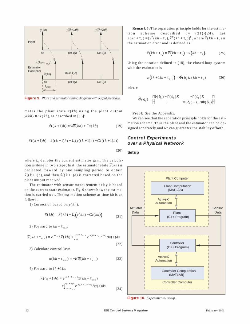
To show the influence of networks on control system perfor-mance and to test the compensation and control strategies,control experiments over a physical network were per-formed. This experiment allows real network traffic to be in-volved in the feedback control of the plant. Theexperimental setup is shown in Fig. 10.

For our experiments, we use the Case Western ReserveUniversity campus-wide network (CWRUnet), which is awide-area network containing both Ethernet and ATM at thephysical layer. Communication between nodes is done us-ing TCP/IP sockets (at the transport and network layer, re-spectively). TCP/IP sockets provide reliable transmission ofdata packets, regardless of possible collisions that mighthappen on the physical transmission medium. Therefore,TCP/IP will result in packet delay but not packet loss.

In our control setup, two computers, working as plant andcontroller, respectively, are connected over CWRUnet. Eachcomputer runs a Visual C++ program as the user interface forsetting up the sockets between them and accepting variousconfiguration parameters, such as sampling period, controlwith estimation, and clock synchronization. The computa-tion for simulating the plant and controller is carried out us-ing MATLAB; that is, MATLAB works as a computation enginefor each program on its own computer. MATLAB is invoked asan ActiveX automation server. On the plant computer, theC++ program obtains the control signal from the network,passes it to MATLAB for plant state and output calculation,and then sends the plant output to the controller computer.On the controller computer, the C++ program obtains theplant output from the network, uses MATLAB to calculate thecontrol signal, and sends the signal to the plant computer. Inthis way, sensor data and control data are passed on the net-work, along with other campus network traffic, and may ex-perience collision or delay.

For a detailed description of an alternate experimentaltestbed for controlling systems over the Internet, see [18].

Clock SynchronizationIn the experiment, every message sent out by the plant andcontroller is time stamped. To calculate the delay accu-rately, plant and controller clocks must be synchronized.

Clock synchronization can be achieved in several ways,such as software synchronization, hardware synchroniza-tion, or a combination of the two. Clock synchronization inour experiment has been done as in [19]. Suppose the con-troller wants to synchronize its clock with the plant. It sendsa message to the plant, and the plant will send its clock read-ing back to the controller. The controller records the clockoffset and the round-trip time. The measurement is carriedout many times, and the controller uses the clock offset withthe minimum round-trip time.

An ExampleThe following example illustrates the effectiveness of thecompensation scheme described above.

Example 4: Consider the state-space plant model

[ ]

x

x

x

xu

yx

1

2

1

2

0 5

0 0

0

1

1 0

=

+

= 1

2x

.

A state feedback controller is u Kx= − , where K = [ , ]25 10(closed-loop poles at − ±5 10 j).

The plant and controller are implemented in twoMATLAB M-files that run on two computers, as describedabove. The plant state x t( ) and the control signal u t( ) aresent using TCP/IP sockets. A scaled step response usingfull-state feedback is shown in Fig. 11, with comparison tothe nonnetworked sampled data system. Network-induceddelay causes the closed-loop plant to be underdamped, re-sulting in larger overshoot in the step response. After using

February 2001 IEEE Control Systems Magazine 93

1.6

1.4

1.2

1

0.8

0.6

0.4

0.2

0

Out

put

w/o Delayw/ Networkw/ Estimation

0 0.5 1 1.5 2

Time (s)

Figure 11. Comparison of scaled step responses with full-statefeedback.

w/o Delayw/ Networkw/ Estimation

1.6

1.4

1.2

1

0.8

0.6

0.4

0.2

0

Out

put

0 0.5 1 1.5 2Time (s)

Figure 12. Comparison of scaled step responses with unmodelednonlinearity.

delay compensation, the response is very similar to thenonnetworked system. Indeed, the difference is caused bythe controller-to-actuator delay, which is not compensatedby this scheme.

This linear estimator also works well when there is anunmodeled nonlinearity in the plant model. For example,consider the plant

( ), .

x x

x u1 2

2

5==

sin

The experimental result, shown in Fig. 12, illustrates that thecompensation scheme still works well.

Stability of NCSwith Data Packet DropoutWhen using an NCS, one must consider not only net-work-induced delay, but also data packet dropout. Net-works can be viewed as unreliable data transmission paths,where packet collision and network node failure occasion-ally occur. When there is a packet collision, instead of re-peated retransmission attempts, it might be advantageousto drop the old packet and transmit a new one. Thus it isvaluable to analyze the rate (percentage successful) atwhich the data should be transmitted to achieve the desiredperformance (stability).

An NCS with data packet dropout can be modeled as anasynchronous dynamical system (ADS) with rate con-straints on events. The stability of this type of system isstudied in [11]. We will extend a result therein to NCSs.

ADSs with Rate ConstraintsADSs, like hybrid systems, are systems that incorporatecontinuous and discrete dynamics. The continuous dynam-ics are governed by differential or difference equations,whereas the discrete dynamics are governed by finite au-tomata that are driven asynchronously by external discreteevents with fixed rates [11].

We consider a simplified ADS with rate constraints thatcan be described by a set of difference equations

x k f x k s Ns( ) ( ( )), , , ,+ = =1 1 2 ,

with continuous-valued state x k n( ) ∈ R . Here, 1 2, , , N rep-resents the set of discrete states, which has a correspond-ing set of rates r r rN1 2, , , . These rates represent the fractionof time that each discrete state occurs; thus Σi

Nir= =1 1.

The stability of such an ADS is given by the following the-orem.

Theorem 6 [11]: Given an ADS as defined above. If thereexist a Lyapunov function V x k n( ( )):R R→ + and scalarsα α α1 2, , , N corresponding to each rate such that

α α α α1 21 2 1r r

NrN⋅ ⋅ ⋅ > > (27)

and

( )V x k V x k V x k s Ns( ( )) ( ( )) ( ( )), , , , ,+ − ≤ − =−1 1 1 22α

(28)then the ADS remains exponentially stable, with decay rategreater than α .

Theorem 6 requires the ADS to be stable on the average.It does not require every difference equation of the ADS tobe stable, but rather it guarantees the ADS to be stable onthe whole. If the discrete state dynamics is given byx k h x khs(( ) ) ( )+ =1 Φ for s N=1 2, , , , the search for theLyapunov function of type V x kh x kh Px khT( ( )) ( ) ( )= andthe scalars α α α1 2, , , N can be cast into a bilinear matrix in-equality (BMI) problem [11]. Equations (27) and (28) can berewritten as

r r rN N1 1 2 2 0log log logα α α+ + ⋅⋅⋅ + >

and

Φ ΦsT

s sP P s N≤ =−α 2 1 2, , , , .

This is a BMI problem in P and the logα is.

Modeling an NCSwith Data Packet DropoutFig. 13 illustrates an NCS setup with the possibility of drop-ping data packets. Here we assume that the nonnetworkedsystem is stable and the network is only inserted from theplant to the controller. The network can be modeled as aswitch that closes at a certain rate r. When the switch isclosed (position S1), the network packet containing x kh( ) istransmitted, whereas when it is open (position S2), the out-put of the switch is held at the previous value and the packetis lost. Thus the dynamics of the switch (state x) can bemodeled as

S x kh x kh

S x kh x k h1

2 1

: ( ) ( ),

: ( ) (( ) ).

== −

Let z kh x kh x khT T T( ) [ ( ), ( )]= be the augmented state vec-tor; the closed-loop system with the network packet drop-out effect is represented by

94 IEEE Control Systems Magazine February 2001

x kh( )Φ + Γ u kh( )x k h(( +1) ) =

x kh( )

1S 2S

ControllerK x kh( )

Plant x kh( )

Figure 13. NCS with data packet dropout.

z k h z khs(( ) )~

( )+ =1 Φ

for s =1 2, . When the switch is in position S1,

~;Φ

Φ ΓΦ Γ1 =

−−

K

K

when the switch is position S2,

~.Φ

Φ Γ2 0

=−

K

I

Normally, a feedback control system can tolerate a certainamount of feedback data loss. The following corollary can beused to test the system stability for a certain rate of data loss.

Corollary 7: For the above system setup, assume theplant state x kh( )is transmitted at the rate of r. If there exist aLyapunov functionV x kh x kh Px khT( ( )) ( ) ( )= and scalars α 1

and α 2 such that

α ααα

1 21

1 1 12

2 2 22

1r r

T

T

P P

P P

−

−

−

>≤≤

,~ ~

,~ ~Φ ΦΦ Φ

the system is still exponentially stable.With the plant state being transmitted at rate r, the effec-

tive sampling period becomes h h reff = / . This suggests thatthe plant can be stabilized by a slower sampling rate. Inother words, the result shows that when we have fast sam-pling, we can drop the samples at a certain rate to save net-work bandwidth and still provide a stable feedback controlsystem.

Example 5: Consider the state-space plant model in Ex-ample 1. When the plant is sampled with a sampling periodh = 0 3. s, we obtain

Φ Γ=

=

10 0 2955

0 0 9704

0 0167 0 0512

01108 0 33

. .

.,

. .

. .K

99

,

and the closed-loop system ( )Φ Γ− K is still stable with thecontinuous controller. With the setup shown in Fig. 13, andassuming the transmission rate r = 0 7. , we solve the LMIproblem [20], [21] in Corollary 7 to find

α α1 211288 0 7552= =. , .

and

P =

− −− −

0 9210 0 9196 0 6578 0 5144

0 9196 24788 0 5232 1

. . . .

. . . .6644

0 6578 0 5232 0 7003 0 6461

0 5144 16644 0 6461

− −− −

. . . .

. . . 20562.

,

which proves the stability of the system. This means thatwhen the plant state is sampled every 0.3 s, if 70% of the pack-ets are delivered to the controller, we can still guarantee thestability of the feedback control system. The result shows aneffective sampling period of h h reff = =/ .0 43 s; in fact, the max-imum stable constant sampling period for this system is 1.7 s.The comparison of step responses with packet dropouts isshown is Fig. 14. We can see that the step response with 70%packets transmitted is similar to the original system. A largedifference can be seen when only 20% of packets are transmit-ted (but the system is still stable, as we prove below).

The setup in Fig. 13 has also been considered by Walsh etal. [3], who used a different approach to determine the MATIτ when the feedback loop is closed over the network. Usingthis conservative approach, the MATI τ of this example is4 5 10 4. × − s, which will consume a lot of network bandwidth ifit is implemented in a real application. The method pre-sented here takes a probabilistic approach while guarantee-ing the exponential stability of the NCS, and it only requiresplant state to be transmitted at a certain rate. This reducesnetwork traffic without sacrificing stability.

The lower the transmission rate, the less network band-width used. The next question would be, “What is the lowerbound on transmission rate r that still guarantees the stabil-ity of the system?” Theorem 8 involves the bound on thetransmission rate r for a stable NCS.

Theorem 8: Consider the setup of Fig. 13, assuming thatthe closed-loop system with no dropout is stable (i.e.,Φ Γ− Kis Schur).

• If the open-loop system (Φ) is marginally stable, thenthe system is exponentially stable for all 0 1< ≤r .

• If the open-loop system is unstable, then the system isexponentially stable for all

11

11 2−

< ≤γ γ/

r

where

February 2001 IEEE Control Systems Magazine 95

w/o Packet Dropoutw/ 70% Packets Transmittedw/ 20% Packets Transmitted

1.4

1.2

1

0.8

0.6

0.4

0.2

00 5 10 15 20 25 30

Time (s)

Out

put

Figure 14. Comparison of scaled step responses with packetdropouts.

[ ] [ ]γ λ γ λ12

22= − =log ( ) , log ( ) .max maxΦ Γ ΦK

Proof: See the Appendix.

Example 6: Example 5 hasΦ marginally stable, so the net-worked controller is stable for all r > 0.

Modeling an NCSwith Multiple-Packet TransmissionAn NCS with multiple-packet transmission can also be mod-eled as an ADS. In multiple-packet transmission mode, plantstate or output are split into separate packets. Fig. 15 illus-trates a case where the plant state is transmitted in twopackets. The dynamics of the network is given by

S x kh x kh x kh x k h

S x kh x k1 1 1 2 2

2 1 1

1: ( ) ( ), ( ) (( ) ),

: ( ) ((

= = −= − =1 2 2) ), ( ) ( ).h x kh x kh

Assume

x kh x kh x khT T T( ) [ ( ), ( )] , ,= =

=

1 211 12

21 22

1

ΦΦ ΦΦ Φ

ΓΓΓ2

1 2

=, [ , ].K K K

Let the augmented state be ( ) ( )[ ( )z kh x kh x khT T= 1 2, ,x kh x khT T T

1 2( ), ( )] . We can now write the closed-loop systemwith two-packet transmission as

z k h z khs(( ) )~

( )+ =1 Φ

for s =1 2, . When the switch is at S1,

~Φ

Φ Φ Γ ΓΦ Φ Γ ΓΦ Φ Γ Γ1

11 12 1 1 1 2

21 22 2 1 2 2

11 12 1 1 1

=

− −− −− −

K K

K K

K K

I2

0 0 0

,

whereas when the switch is at S2,

~Φ

Φ Φ Γ ΓΦ Φ Γ Γ

Φ Φ Γ

2

11 12 1 1 1 2

21 22 2 1 2 2

21 22 2

0 0 0=

− −− −

−

K K

K K

I

K 1 2 2−

Γ K

.

The modeling can be easily extended to systems withmore than two packets.

Stability in Scheduling NetworksWe know that in scheduling networks, packets are sent outsequentially in a predetermined order, as shown in Fig. 16.The packet sequence received by the controller isx x x x1 2 1 2→ → → → ⋅⋅⋅.

Remark 9: If~ ~Φ Φ1 2⋅ is Schur, the NCS with static schedul-

ing of transmitting plant states is exponentially stable.This shows that it is not necessary to ensure that both

~Φ 1

and~Φ 2 are Schur. The NCS is stable if

~ ~Φ Φ1 2⋅ is Schur, as thefollowing example illustrates.

Example 7: Consider the system in Example 5 with theplant state x x1 2, transmitted separately in two packets.With h = 0 3. s, we have

~

. . . .

. . .

.Φ 1

10 0 2995 0 0167 0 0512

0 0 9704 01108 0 3399

1=

− −− −

0 0 2995 0 0167 0 0512

0 0 10 010 0 29

2

. . .

.

~

. .

− −

=Φ

95 0 0167 0 0512

0 0 9704 01108 0 3399

0 0 10 0

0 0 9704

− −− −

. .

. . .

.

. − −

01108 0 3399. .

.

Neither~Φ 1 nor

~Φ 2 is Schur; however,~ ~Φ Φ1 2⋅ is Schur,

which proves the stability of the system if a scheduling net-work is applied.

Using static scheduling on this two-packet setup, eachpacket is transmitted 50% of the time; thus the effectivesampling period is h heff = =/ . .0 5 0 6 s. The step response ofthis two-packet transmission setup is similar to the origi-nal system.

ConclusionsThis article analyzed several fundamental issues in networkcontrol systems. One issue is the network-induced delaywhen transmitting sensor data and control data. Dependingon the control network protocol employed, the delay can beeither constant or time varying. The relationship between

96 IEEE Control Systems Magazine February 2001

x kh( )2

x kh( )1

1S

2S

= Φ x kh( ) +x k h(( +1) ) u kh( )Γ

T1

T2

x kh x kh x kh( ) = ( ), ( )[ ]TK x kh( )Controller

Plant

–

Figure 15. NCS with multiple-packet transmission.

x1x2 x1 x2

...kh ( +1)k h ( +3)k h( +2)k h

Figure 16. Multiple-packet transmission with static scheduling.

February 2001 IEEE Control Systems Magazine 97

the sampling rate h and the network-induced delay τ wascaptured using a stability region plot. Stability of an NCS wasalso characterized using a hybrid systems stability analysistechnique. Methods to compensate network-induced delayusing the time-domain solution of the plant model were dis-cussed, and experimental results over a physical network(CWRUnet) were presented. We then modeled an NCS withpacket dropout and multiple-packet transmission (whichmay occur due to the limitation of the control network) asan asynchronous dynamical system. We determinedwhether the NCS is stable at a certain rate of data loss, andwe searched for the highest rate of data loss for the NCS tobe stable.

References[1] Y. Halevi and A. Ray, “Integrated communication and control systems:Part I—Analysis,” J. Dynamic Syst., Measure. Contr., vol. 110, pp. 367-373, Dec.1988.[2] J. Nilsson, “Real-time control systems with delays,” Ph.D. dissertation,Dept. Automatic Control, Lund Institute of Technology, Lund, Sweden, Janu-ary 1998.[3] G.C. Walsh, H. Ye, and L. Bushnell, “Stability analysis of networked controlsystems,” in Proc. Amer. Control Conf., San Diego, CA, June 1999, pp. 2876-2880.[4] M.S. Branicky, S.M. Phillips, and W. Zhang, “Stability of networked controlsystems: Explicit analysis of delay,” in Proc. Amer. Control Conf., Chicago, IL,June 2000, pp. 2352-2357.[5] W. Lawrenz, CAN System Engineering: From Theory to Practical Applica-tions. New York: Springer-Verlag, 1997.[6] A.S. Tanenbaum, Computer Networks, 3rd ed. Upper Englewood Cliffs, NJ:Prentice-Hall, 1996.[7] D. Anderson, FireWire System Architecture. Reading, MA: Addison-Wesley,1998.[8] E. Altman, T. Bas,ar, and R. Srikant, “Congestion control as a stochastic con-trol problem with action delays,” Automatica, vol. 35, pp. 1937-1950, Dec. 1999.[9] S. Mascolo, “Classical control theory for congestion avoidance inhigh-speed Internet,” in Proc. IEEE Conf. Decision and Control, Phoenix, Dec.1999, pp. 2709-2714.[10] L. Dugard and E.I. Verriest, Eds., Stability and Control of Time-Delay Sys-tems (Lecture Notes in Control and Information Sciences), vol. 228. Heidel-berg, Germany: Springer-Verlag, 1997.[11] A. Hassibi, S.P. Boyd, and J.P. How, “Control of asynchronous dynamicalsystems with rate constraints on events,” in Proc. IEEE Conf. Decision and Con-trol, Phoenix, AZ, Dec. 1999, pp. 1345-1351.[12] J.D. Spragins, J.L. Hammond, and K. Pawlikowski, Telecommunications:Protocols and Designs. Reading, MA: Addison-Wesley, 1991.[13] M. Tangemann and K. Sauer, “Performance analysis of the timed tokenprotocol of FDDI and FDDI-II,” IEEE J. Select. Areas Commun., vol. 9, pp.271-278, Feb. 1991.[14] K.J. Åström and B. Wittenmark, Computer-Controlled Systems: Theory andDesign, 3rd ed. Englewood Cliffs, NJ: Prentice-Hall, 1997.[15] G.F. Franklin, J.D. Powell, and M. Workman, Digital Control of Dynamic Sys-tems, 3rd ed. Reading, MA: Addison Wesley Longman, 1997.[16] M.S. Branicky, “Hybrid systems: Modeling, analysis, and control,” Sc.D.dissertation, Dept. Electrical Engineering and Computer Science, Massachu-setts Institute of Technol., Cambridge, MA, June 1995.[17] M.S. Branicky, “Stability of hybrid systems: State of the art,” in Proc. IEEEConf. Decision and Control, San Diego, CA, Dec. 1997, pp. 120-125.[18] J.W. Overstreet and A. Tzes, “An Internet-based real-time control engi -neering laboratory,” IEEE Contr. Syst. Mag., vol. 19, pp. 19-34, Oct. 1999.[19] D. Mills, “Internet time synchronization: The network time protocol,”IEEE Trans. Commun., vol. 39, pp. 1482-1493, Oct. 1991.[20] S. Boyd, L. El Ghaoui, E. Feron, and V. Balakrishnan, Linear Matrix Inequal-ities in System and Control Theory. Philadelphia, PA: SIAM, 1994.[21] P. Gahinet, A. Nemirovshi, A. Laub, and M. Chilali, MATLAB LMI ControlToolbox. Natick, MA: MathWorks, May 1995

[22] G.H. Golub and C.F. Van Loan, Matrix Computations, 3rd ed. Baltimore,MD: Johns Hopkins Univ. Press, 1996.

AppendixProof (Corollary 2): Throughout, we use vector and ma-

trix norm definitions and inequalities [22].The Lyapunov function V x( ) must satisfy the following

inequalities:

λ λ

λ1

22

2

2

x V x x

V x X QX Q xT

≤ ≤

= − ≤ −

( )

( ) ( ) .min

Thus, following the proof of [3, Theorem 2], (8) of [3] shouldbe rewritten as:

( )( ( )) ( ) ( ) ( ) ( ) .V x t x t Q x t A z t≤ − +λ λ γmin 2 2 1 0

Because of the choice of τ,

γ λλ λ λ

λλ1

2 2 1 28 8< ≤min min( )

/( )Q

A

QA

.

The same result as in [3] can then be obtained: for allt t p V x t z t> + <0 2 0

2τ γ, ( ( )) || ( )|| . Setting

γ λλ λ λ1

2 2 1

14 8

<

min ,( )/

min Q

A

we still have V x t z t e t z t( ( )) ( ) , ( ) ( )< <γ γ2 02

1 0 for allt t p> +0 τ.

Viewing the NCS as perturbed by the bounded error sig-nal e t( ), consider the system

( ) ( ) ( )x t A x t A e tz z= +11 12

star ting at t t p= +0 τ with zero init ial conditionx t p( )0 0+ =τ . We can conclude that for all t t p> +0 τ,

V x tA z t

Q

x tA

z z

z

( ( ))( )

( )

( )/

<

<

4

2

23 2

12

0

2

2 2 1 1

λ γλ

λ λ λ γ

2min

z t

Q

( )

( )0

λmin

and, by the choice of γ1 above, x t z tz ( ) ( / ) ( )< 1 4 0 . The restof the proof for this part continues as in [3].

We now proceed to prove that the third bound is alwaysthe smallest among the three terms above. We first prove

1

8 1

2

2 1 1A i p A

i

p( / )

ln( )

λ λ +<

=∑.

We know that λ λ2 1 1/ ≥ , i p pi

p= +

=∑ ( ) /1 21

and p ≥1, hence

1

8 1

18 1

18

2 1 1A i A p p p A

i

p( / ) ( )λ λ +

≤+

<=∑

.

Since ln( )2 is greater than 0.125,

ln( )2 18p A p A

>

and the result follows. We then can prove

λλ λ λ λ λ

λ λ

min( )

/ ( / )

( / )

Q

A i

A i

i

p

i

16 1

1

8 1

2 2 12

2 1 1

2 1 1

+

≤+

=

=

∑p∑

.

Canceling common terms, we must show

λλ λ λ

min( )/Q

A21

2 2 1

≤ .

Since λ λ2 1 1/ ≥ by definition, it is enough to show

λλ

min( )QA2

12

≤ .

Taking norms on both sides of (3), we obtain

− = +≤ +=

Q A P PA

A P P A

P A

T

T

11 11

11 11

112

where the inequality follows from the triangle inequalityplus the submultiplicative property of the matrix 2-norm.Now, since P is posit ive-definite symmetric,P P= =λ λmax ( ) 2. Also, A A≥ 11 follows easily from the def-inition of the induced norm, since the latter is a submatrix ofthe former (cf. (2)). Therefore,

λ λmin( )Q Q A≤ − ≤ 2 2

and

λλ

min( )QA2

12

≤ .

Q.E.D.Proof (Corollary 5): The plant model is given by

( )x k h x kh u khsc k k sc k k sc k( ) ( ) ( ) ( ) ( ), , ,+ + = + + ++1 1τ δ τ δ τΦ Γ ,

where δk , Φ( )δk , and Γ( )δk are given (18).The estimation scheme is given by (21)-(24); from (21)

and (24) we have

x k h e x kh

e B ds u

A hsc k

Ash

sc k

sc k

(( ) ) ( )

(

( ),

,

,

+ = +

+

−

−∫1

0

τ

τ

τ

( )kh

L He x kh x kh

sc k

cA h

sc k sc ksc k

+

+ + − +−

τ

τ ττ

,

( ), ,

)

( ) ( ),

and from (22) we have

( )x k h x kh

u khsc k k sc k

k sc k

( ) ( ) ( )

( ) ( ), ,

,

+ + = +

+ +

+

+1 1τ δ τ

δ τ

Φ

Γ

()

L H x kh

x kh

c k sc k

sc k

Φ( ) ( )

( ) .

,

,

δ τ

τ

+

− +

The estimation error is defined in (25), and the error equa-tion is

( ) ( ) ( )~ ( ) ( ) ( ) ~, ,x k h L H x khsc k k c k sc k+ + = − ++1 1τ δ δ τΦ Φ .

(29)Now apply the control law to form the closed-loop sys-

tem

u kh Kx khsc k sc k( ) ( ), ,+ = − +τ τ .

The closed-loop system is

( ) ( )( )

x k h x kh

Kx kh

sc k k sc k

k sc k

( ) ( )

( )

(

, ,

,

+ + = +

− +=

+1 1τ δ τ

δ τδ

Φ

ΓΦ( ) ( )

( )k k sc k

k sc k

K x kh

Kx kh

) ( )

( ) ~ .

,

,

− +

− +

Γ

Γ

δ τ

δ τ (30)

Combining (29) and (30), we have (26).Q.E.D.

Proof (Theorem 8): Consider the setup of Corollary 7,and define β αi i= −2 for i =1 2, . Substituting and taking logs, ifthe transmission rate r satisfies

loglog log

ββ β

2

2 1

1−

< ≤r(31)

where β1 1< andβ β2 1> are positive constants and P is a pos-itive-definite symmetric matrix such that

~ ~,

~ ~Φ Φ

Φ Φ1 1 1

2 2 2

T

T

P P

P P

≤

≤

β

β

the system is exponentially stable.Transmission rate r depends onβ1 andβ2, and the choice

of β1, β2 must satisfy β λ12

1≥ max (~

)Φ and β λ22

2≥ max (~

)Φ .Looking at (31), it makes sense to minimize both logβ2

and logβ1 0< to obtain the weakest lower bound on rpossible from that equation.

Now note that

98 IEEE Control Systems Magazine February 2001

( )λ λmax max

~( )2

12Φ Φ Γ= − K ,

since the two matrices share the same spectrum (althougheach eigenvalue of the former has twice the multiplicity ofthe latter). Also note that the block-diagonal structure of

~Φ 2

implies

( ) λ λmax max

~max , ( )2

221Φ Φ= ,

with one achieving the maximum if and only if Φ is stable.The theorem is now seen to easily follow.

Q.E.D.

Wei Zhang received his B.S. and M.S. degrees in electricalengineering from Tianjin University, Tianjin, China, in 1993and 1996, respectively. He then worked for the Industrial Au-tomation and Control Division of Honeywell (Tianjin) Ltd. asa Systems Engineer from 1996 to 1997. He is now pursuinghis Ph.D. degree in electrical engineering and computer sci-ence at Case Western Reserve University. His research inter-ests include the modeling, analysis, and design ofnetworked control systems.

Michael S. Branicky received the B.S. (1987) and M.S.(1990) degrees in electrical engineering and applied physics

from Case Western Reserve University (CWRU). In 1995, hereceived his Sc.D. in electrical engineering and computerscience from the Massachusetts Institute of Technology. In1997, he rejoined CWRU as an Assistant Professor of Electri-cal Engineering and Computer Science. He has held re-search positions at MIT’s AI Lab, Wright-Patterson AFB,NASA Ames, Siemens Corporate Research (Munich), andLund Institute of Technology’s Dept. of Automatic Control.His research interests include hybrid systems, intelligentcontrol, and learning, with applications to robotics, flexiblemanufacturing, and control over networks.

Stephen M. Phillips received the B.S. degree with distinctionin electrical engineering from Cornell University in 1984 andthe M.S. and Ph.D. degrees in electrical engineering fromStanford University in 1985 and 1988, respectively. He joinedthe faculty of Case Western Reserve University in 1988, wherehe is currently Associate Professor in the Department of Elec-trical Engineering and Computer Science. He serves as Direc-tor of the Center for Automation and Intelligent Systems andis a registered professional engineer. His research interestsinclude sampled-data control, system identification, andadaptive control, with applications to manufacturing, aero-space, and microelectromechanical systems.

February 2001 IEEE Control Systems Magazine 99