STABILITY ANALYSIS OF PIPE RACKS FOR INDUSTRIAL FACILITIES By David A. Nelson B.S., Walla Walla University, 2008 A thesis submitted to University of Colorado Denver in partial fulfillment of the requirements for the degree of Master of Science, Civil Engineering 2012

Welcome message from author
This document is posted to help you gain knowledge. Please leave a comment to let me know what you think about it! Share it to your friends and learn new things together.
Transcript

STABILITY ANALYSIS OF PIPE RACKS FOR INDUSTRIAL FACILITIES
By
David A. Nelson
B.S., Walla Walla University, 2008
A thesis submitted to
University of Colorado Denver
in partial fulfillment
of the requirements for the degree of
Master of Science, Civil Engineering
2012

This thesis for the Master of Science
degree by
David A. Nelson
has been approved
by
Fredrick Rutz
Kevin Rens
Rui Liu

Nelson, David A. (M.S., Civil Engineering)
Stability Analysis of Pipe Racks for Industrial Facilities
Thesis directed by Professor Fredrick Rutz
ABSTRACT Pipe rack structures are used extensively throughout industrial facilities
worldwide. While stability analysis is required in pipe rack design per the AISC
Specification for Structural Steel Buildings (AISC 360-10), the most compelling
reason for uniform application of stability analysis is more fundamental. Improper
application of stability analysis methods could lead to unconservative results and
potential instability in the structure jeopardizing the safety of not only the pipe rack
structure but the entire industrial facility.
The direct analysis method, effective length method and first order method are
methods of stability analysis that are specified by AISC 360-10. Pipe rack structures
typically require moment frames in the transverse direction creating intrinsic
susceptibility to second order effects. This tendency for large second order effects
demands careful attention in stability analysis. Proper application as well as clear a
understanding of the limitations of each method is crucial for accurate pipe rack
design.

A comparison of the three AISC 360-10 methods of stability analysis was
completed for a representative pipe rack structure using the 3D structural analysis
program STAAD.Pro V8i. For the model chosen, all three methods of stability
analysis met AISC 360-10 requirements.
For typical pipe rack structures, all three methods of stability analysis are
acceptable as long as limitations are met and the methods are applied correctly. The
first order method typically provided conservative results while the effective length
method was determined to underestimate the moment demand in beams or
connections that resist column rotation. The direct analysis method was found to be a
powerful analysis tool as it requires no additional calculations to calculate additional
notional loads, calculate effective length factors or verify AISC 360-10 limitations.
This abstract accurately represents the content of the candidate’s thesis. I recommend
its publication.
Fredrick Rutz

ACKNOWLEDGEMENT
I would like to thank first and foremost Dr. Fredrick Rutz for the support and
guidance in completion of this thesis. I would also like to thank Dr. Rens and Dr. Li
for participating on my graduate advisory committee. Lastly, I would like to thank
various work associates for their help with either editing or discussion of the topic.

vi
TABLE OF CONTENTS
LIST OF FIGURES ........................................................................................................... ix
LIST OF TABLES ............................................................................................................ xii
Chapter
1. Introduction ..............................................................................................................1
1.1 Stability Analysis of Steel Structures ......................................................................1
1.2 Pipe Racks in Industrial Facilities............................................................................3
2. Problem Statement ...................................................................................................6
2.1 Introduction ..............................................................................................................6
2.2 Significance of Research..........................................................................................8
2.3 Research Objective ..................................................................................................8
3. Literature Review...................................................................................................10
3.1 Introduction ............................................................................................................10
3.2 Pipe Rack Loading .................................................................................................10
3.2.1 Load Definitions ............................................................................................10
3.2.2 Dead Loads ....................................................................................................14
3.2.3 Live Loads .....................................................................................................15
3.2.4 Thermal and Self Straining Loads .................................................................16
3.2.5 Snow Load and Rain Loads ...........................................................................16

vii
3.2.6 Wind Loads ....................................................................................................17
3.2.7 Seismic Loads ................................................................................................21
3.2.8 Load Combinations ........................................................................................22
3.3 Column Failure and Euler Buckling ......................................................................25
3.4 Stability Analysis ...................................................................................................29
3.4.1 AISC Specification Requirements .................................................................29
3.4.2 Second Order Effects .....................................................................................29
3.4.3 Flexural, Shear and Axial Deformation .........................................................34
3.4.4 Geometric Imperfections ...............................................................................35
3.4.5 Residual Stresses and Reduction in Stiffness ................................................37
3.5 AISC Methods of Stability Analysis......................................................................41
3.5.1 Rigorous Second Order Elastic Analysis .......................................................43
3.5.2 Approximate Second Order Elastic Analysis ................................................46
3.5.3 Direct Analysis Method .................................................................................47
3.5.4 Effective Length Method ...............................................................................52
3.5.5 First Order Method ........................................................................................58
4. Research Plan .........................................................................................................61
5. Member Design ......................................................................................................63
6. Pipe Rack Analysis ................................................................................................68
6.1 Generalized Pipe Rack ...........................................................................................68
6.2 Pipe Rack Loading .................................................................................................72

viii
6.3 Pipe Rack Load Combinations...............................................................................83
6.4 Strength and Serviceability Checks .......................................................................86
6.5 Base Support Conditions........................................................................................87
6.6 Effective Length Factor .........................................................................................88
6.7 Notional Load Development for First Order Method ............................................91
6.8 STAAD Benchmark Validation .............................................................................93
7. Comparison of Results ...........................................................................................96
8. Conclusions ..........................................................................................................111
References ........................................................................................................................116
Appendix A – STAAD Input Pinned Base Analysis - Effective Length Method ...........123
Appendix B – STAAD Input Pinned Base Analysis - Direct Analysis Method ..............132
Appendix C – STAAD Input Pinned Base Analysis - First Order Method .....................141

ix
LIST OF FIGURES
Figure
1-1 Typical Four-Level Pipe Rack Consisting of Eight Transverse Frames
Connection by Longitudinal Struts ....................................................................4
2-1 Typical Elevation View of Pipe Rack ................................................................7
2-2 Section View Showing Moment Resisting Frame .............................................7
3-1 Load vs. Deflection – Yielding of Perfect Column .........................................26
3-2 Visual Definition of Critical Buckling Load Pcr ..............................................27
3-3 Load vs. Deflection – Euler Buckling..............................................................28
3-4 Second Order P-δ and P-Δ moments (Adapted from Ziemian, 2010) .............30
3-5 Comparison of First Order Analysis to Second Order Analysis (Adapted from
Gerschwindner, 2009) ......................................................................................31
3-6 Quebec Bridge Prior to Collapse (Canada, 1919) ............................................32
3-7 Quebec Bridge after Failure (Canada, 1919) ...................................................33
3-8 Deformation from Flexure, Shear and Axial (Adapted from Gerschwindner,
2009) ................................................................................................................35
3-9 Load vs. Deflection – Real Column Behavior with Initial Imperfections .......37
3-10 Residual Stress Patterns in Hot Rolled Wide Flange Shapes ..........................38
x
3-11 Influence of Residual Stress on Average Stress-Strain Curve (Salmon and
Johnson, 2008) .................................................................................................39
3-12 Idealized Residual Stresses for Wide Flange Shape Members – Lehigh Pattern
(Adapted from Ziemian, 2010) ........................................................................40
3-13 Load vs. Deflection – Comparison of Analysis Types (Adapted from White
and Hajjar, 1991) .............................................................................................42
3-14 Visual Representation of Incremental-Iterative Solution Procedure (Adapted
from Ziemian, 2010) ........................................................................................45
3-15 Reduced Modulus Relationship (Powell, 2010) ..............................................52
3-16 Alignment Chart – Sidesway Inhibited (Braced Frame) (Adapted from AISC
360-10) .............................................................................................................54
3-17 Alignment Chart – Sidesway Uninhibited (Moment Frame)
(Adapted from AISC 360-10) ..........................................................................55
5-1 Simple Cantilever Design Example .................................................................64
5-2 Simple Cantilever Design Example Results ....................................................66
6-1 Isometric View of Typical Pipe Rack Structure Used for Analysis ................70
6-2 Section View of Moment Frame in Typical Pipe Rack ...................................71
6-3 Section View of Moment Frame – Operating Dead Load ...............................74
6-4 Section View of Moment Frame – Pipe Anchor Load ....................................77

xi
6-5 Section View of Moment Frame – Wind Load ................................................81
6-6 Section View of Moment Frame – Operating Seismic ....................................83
6-7 Effective Length Factor K – Pinned Base ........................................................90
6-8 Effective Length Factor K – Fixed Base ..........................................................91
6-9 AISC Benchmark Problems (Adapted from AISC 360-10) ............................94

xii
LIST OF TABLES
Table
3-1 Force coefficient, Cf for open structures trussed towers (Adapted from ASCE
7-05) .................................................................................................................18
3-2 Cf force coefficient (Adapted from ASCE 7-05) ...........................................20
3-3 Comparison of direct analysis method and equivalent length method (Adapted
from Nair, 2009) ..............................................................................................57
6-1 Velocity pressure for cable tray and structural members .................................78
6-2 Velocity pressure for pipe ................................................................................79
6-3 Resultant design wind force from pipe ............................................................80
6-4 Lateral seismic forces – operating ...................................................................82
6-5 Lateral seismic forces – empty ........................................................................82
6-6 Benchmark solutions ........................................................................................95
7-1 Ratio Δ2/Δ1 effective length method – pinned base .........................................97
7-2 Ratio Δ2/Δ1 direct analysis method – pinned base ...........................................99
7-3 Maximum demand to capacity ratio – pinned base .......................................100
7-4 Maximum demand forces – pinned base .......................................................101
7-5 Ratio Δ2/Δ1 effective length method – fixed base ..........................................103

xiii
7-6 Ratio Δ2/Δ1 direct analysis method – fixed base ............................................104
7-7 Maximum demand to capacity ratio – fixed base ..........................................105
7-8 Maximum demand forces – fixed base ..........................................................105
7-9 Ratio Δ2/Δ1 effective length method – pinned base serviceability limits .......107
7-10 Ratio Δ2/Δ1 direct analysis method – pinned base serviceability limits .........108
7-11 Maximum demand to capacity ratio – pinned base serviceability limits .......109

1
1. Introduction
1.1 Stability Analysis of Steel Structures
The engineering knowledge base continues to grow and expand. This growth
creates on-going challenges as designs demand adaptation in response to new
information and technology. Although the value of stability analysis has long been
recognized, implementation in design has historically been difficult as calculations
were performed primarily by hand. Various methods were created to simplify the
analysis and allow the engineer to partially include the effects of stability via hand
calculations. However, with the development of powerful analysis software, rigorous
methods to account for stability effects were developed. While stability analysis
calculations can still be done by hand, most engineers now have access to software
that will complete a rigorous stability analysis. The majority of the methods
presented here assume that software analysis is utilized.
Stability analysis is a broad term that covers many aspects of the design
process. According to the 2010 AISC Specification for Structural Steel Buildings
(AISC 360-10) stability analysis shall consider the influence of second order effects
(P-Δ and P-δ effects), flexural, shear and axial deformations, geometric
imperfections, and member stiffness reduction due to residual stresses.

2
Both the 2005 and 2010 AISC Specification for Structural Steel Buildings
recognize at least three methods for stability analysis: (AISC 360-05 and AISC 360-
10)
1. First-Order Analysis Method
2. Effective Length Method
3. Direct Analysis Method
Other methods for analysis may be used as long as all elements addressed in the
prescribed methods are considered.
Stability analysis is required for all steel structures according to AISC 360-10.
The application of methods for stability analysis in design of structures varies greatly
from firm to firm and from engineer to engineer. A crucial principle for engineers in
the process of design is the inclusion of stability analysis in design. If stability
analysis is not performed or a method of analysis is incorrectly applied, the ability of
the structure to support the required load is potentially jeopardized. The analysis of
nearly all complex structures is completed using advanced analysis software capable
of performing various methods of analysis. Therefore omitting stability analysis in
the design of structures creates unnecessary risk and is unjustified.

3
1.2 Pipe Racks in Industrial Facilities
Pipe racks are structures used in various types of plants to support pipes and
cable trays. Although pipe racks are considered non-building structures, they should
still be designed with the effects of stability analysis considered.
Pipe racks are typically long, narrow structures that carry pipe in the
longitudinal direction. Figure 1-1 shows a typical pipe rack used in an industrial
facility. Pipe routing, maintenance access, and access corridors typically require that
the transverse frames are moment-resisting frames. The moment frames resist
gravity loads as well as lateral loads from either pipe loads or wind and seismic loads.
The transverse frames are typically connected using longitudinal struts with one bay
typically braced. Any longitudinal loads are transferred to the longitudinal struts and
carried to the braced bay. (Drake and Walter, 2010)

4
Figure 1-1 Typical Four-Level Pipe Rack Consisting of Eight Transverse Frames Connection by
Longitudinal Struts
Pipe racks are essential for the operation of industrial facilities but because
pipe racks are considered non-building structures, code referenced documents will
usually not cover the design and analysis of the structure. The lack of industry
standards for pipe rack design leads to each individual firm or organization adopting
its own standards, many without clear understanding of the concepts and design of
pipe rack structures. (Bendapodi, 2010) Process Industry Practices Structural Design
Criteria (PIP STC01015) has tried to develop a uniform standard for design but it
should be noted that this is not considered a code document.

5
The lack of code referenced documents can lead to confusion in the design of
pipe racks. The concept of stability analysis should not be ignored based the lack on
code referenced documents AISC 360-10 should still be used as reference for stability
analysis and design.
6
2. Problem Statement
2.1 Introduction
Industrial facilities typically have pipes and utilities running throughout the
plant which require large and lengthy pipe racks. Pipe racks not only are used for
carrying pipes and cable trays, but many times defines access corridors or roadways.
It is relatively easy to add a braced bay in the longitudinal direction of a pipe rack
because pipes and utilities run parallel to access roads. It is much more difficult to
add bracing to the pipe rack in the transverse direction because of the potential for
interference with pipes, utilities, corridors and access roads. Therefore moment
connections in the transverse direction of the pipe rack are typically used. Figure 2-1
shows an elevation view of a length of pipe rack. Figure 2-2 shows a section view of
the same pipe rack showing the moment resisting frame.
Pipe racks are a good example of structures that can be subject to large second
order effects. The current AISC 360-10 defines three methods for stability analysis:
1. First Order Analysis Method
2. Effective Length Method
3. Direct Analysis Method
Limitations restrict practical application for certain methods.

7
Figure 2-1 Typical Elevation View of Pipe Rack
Figure 2-2 Section View Showing Moment Resisting Frame

8
2.2 Significance of Research
If stability analysis is not performed or a method is incorrectly applied, this
could jeopardize the ability of the structure to support the required loads.
Most of the current literature on pipe racks discusses the application of loads
and has suggestions on design and layout of pipe racks, while little applicable
information is available on comparing the three methods of stability analysis for pipe
racks. Currently the design engineer must research each method of stability analysis
and decide which method to apply for analysis. After the analysis is completed, the
engineer must then verify that the pipe rack meets all the requirements of the applied
analysis method. If the requirements of AISC 360-10 methods are not met for the
structure, then the engineer must completely reanalyze the structure using a new
method of stability analysis which will meet the requirements. Comparing the
various types of stability analysis will not only show the engineer which method will
provide the most accurate analysis based on method limitations, but will also show
why stability analysis is crucial.
2.3 Research Objective
The main purpose of this thesis will be to analyze various types of pipe rack
structures, compare the results from stability analyses, and describe both positive and
negative aspects of each method of stability analysis as it applies specifically to pipe

9
rack structures. The paper will also look at some of the various issues with applying
each of the methods.
Some engineers are accustomed to braced frames structures, which are not
susceptible to large second order effects, therefore those designers can tend to neglect
or incorrectly apply methods of stability analysis. This thesis will not only show the
importance of stability analysis, but also provide suggestions on practical
implementation of each method. This could potentially save time in analysis and
design because the process of selecting the appropriate stability analysis method will
no longer be based on trial and error but rather on educated considerations that can
easily be verified after analysis.

10
3. Literature Review
3.1 Introduction
This section will focus on review of the available literature on the subject of
both pipe rack loading as well as stability analysis. Literature on the general theory
of stability analysis will be reviewed. The main focus of this literature review will be
on the three methods prescribed by AISC 360-10. Layout and loading guidelines for
pipe racks will also be reviewed as this has a major influence on stability.
3.2 Pipe Rack Loading
3.2.1 Load Definitions
Pipe racks are unique structures that have unique loading when compared to
typical buildings and structure. Pipe racks design is not covered under Minimum
Design Loads for Buildings and Other Structures (ASCE 7-05) or International
Building Code (IBC 2009) however the design philosophies should remain the same
as that for all structures. Most company design criteria and Process Industry Practices
(PIP) documents will list ASCE 7-05 or IBC as the basis for load definition and load
combinations. There are several primary loads which should be considered in the
design of pipe racks in addition to loads defined by ASCE 7-05 or IBC 2009. ASCE
7-05 primary load cases are as follows:

11
Ak = load or load effect arising from extraordinary event A
D = dead load
Di = weight of ice
E = earthquake load
F = load due to fluids with well defined pressures and maximum heights
Fa = flood load
H = load due to lateral earth pressure, ground water pressure, or pressure of
bulk materials
L = live load
Lr = roof live load
R = rain load
S = snow load
T = self-straining force
W = wind load
Wi = wind-on-ice determined in accordance with ASCE 7-05 Chapter 10
According to AISC 360-10, regardless of the method of analysis,
consideration of notional loads is required. The notional loads may be required in all
load combinations if certain requirements of the stability analysis are not satisfied.

12
The magnitude of notional load will vary based on the method used. Therefore the
additional primary load cases per AISC 360-10 are as follows:
N = notional load per AISC, applied in the direction that provides the
greatest destabilizing effect
PIP STC01015 states that pipe racks shall be designed to resist the minimum
loads defined in ASCE 7-05 as well as the additional loads described therein. PIP
STC01015 breaks down the dead load into various categories that are not defined in
ASCE 7-05. In addition, various loads from plant operation are defined and required
for consideration in design.
PIP STC01015 breaks down the ASCE 7-05 Dead Load (D) by dividing the
dead load into the subcategories listed below.
Ds = Structure dead load is the weight of materials forming the structure
(not the empty weight of process equipment, vessels, tanks, piping nor
cable trays), foundation, soil above the foundation resisting uplift, and
all permanently attached appurtenances (e.g., lighting, instrumentation,
HVAC, sprinkler and deluge systems, fireproofing, and insulation,
etc…).
Df = Erection dead load is the fabricated weight of process equipment or
vessels.

13
De = Empty dead load is the empty weight of process equipment, vessels,
tanks, piping, and cable trays.
Do = Operating dead load is the empty weight of process equipment,
vessels, tanks, piping and cable trays plus the maximum weight of
contents (fluid load) during normal operation.
Dt = Test dead load is the empty weight of process equipment, vessels,
tanks, and/or piping plus the weight of the test medium contained in
the system.
PIP STC01015 also provides additional primary load cases from the effects of
thermal loads caused from operational temperatures in the pipes.
T = Self-straining thermal forces caused by restrained expansion of
horizontal vessels, heat exchangers, and structural members in pipe
racks or in structures. This is essentially the same load case as defined
in ASCE 7-05.
Af = Pipe anchor and guide forces.
Ff = Pipe rack friction forces cause by the sliding of pipes or friction forces
cause by the sliding of horizontal vessels or heat exchanges on their
supports, in response to thermal expansion.

14
Seismic loads are also discussed in PIP STC01015. Seismic events can occur
either when the plant is in operation or during shutdown when the pipes are empty.
Therefore two seismic load cases are defined as follows:
Eo = Earthquake load considering the unfactored operating dead load and
the applicable portion of the unfactored structure dead load.
Ee = Earthquake load considering the unfactored empty dead load and the
applicable portion of the unfactored structure dead load.
3.2.2 Dead Loads
Further information on the dead loads specifically for pipe racks is defined in
PIP STC01015. The operating dead load for piping on a pipe rack shall be 40 psf
uniformly distributed over each pipe level. The 40 psf load is equivalent to 8 – inch
diameter, schedule 40 pipes, full of water, at 15 inch spacing. For pipes larger than 8
inch, the actual load of pipe and contents shall be calculated and applied as a
concentrated load.
The empty dead load (De) is defined for checking uplift and minimum load
conditions. Empty dead load (De) is approximately 60% of the operating dead load
(Do) which is equivalent to 24 psf uniformly distributed over each pipe rack level.
This is an acceptable approximation unless calculations indicate a different
percentage should be used. (PIP STC01015)
15
Pipe racks for industrial applications are usually designed with consideration
for potential future expansion. Therefore, additional space or an additional level
should be provided and the rack should be uniformly loaded across the entire width to
account for pipes that may be placed there in the future.
Cable trays are often supported on pipe racks and typically occupy a level
within the rack specifically designated for cable tray. The operating dead load (Do)
for cable tray levels on pipe racks shall be 20 psf for a single level of cable tray and
40 psf for a double level. These uniform loads are based on estimates of full cable
tray over the area of load application. (PIP STC01015)
The degree of usage for cable trays can vary greatly. The empty dead load
(De) should be considered on a case by case basis. Engineering judgment should be
used in defining the cable tray loading, because empty dead load (De) is defined for
checking uplift and minimum load conditions.
3.2.3 Live Loads
Live load should be applied to pipe racks as needed. Pipe racks typically have
very few platform or catwalks. When platforms are required for access to valves or
equipment located on the pipe rack structure, the platform and supporting structure
should be designed in accordance with ASCE 7-05 Live Loads.
16
3.2.4 Thermal and Self Straining Loads
Temperature effects on structural steel members should be included in design.
PIP STC01015 introduces two additional self straining loads. These additional loads
are caused by the operation effects on the pipes. The operational temperatures of
pipes need to be considered in design.
Support conditions of pipes vary greatly and need to be considered in design.
A pipe may be supported to resist gravity only, or may have varying degrees of
restraint from guided in a single direction to fully anchored supports. Pipe stress
analysis can be completed for all the pipes located in the pipe rack. This stress
analysis takes into account the support type and location for each support and
provides individual design forces for each pipe at that specific location. These
resultant pipe loads can be used for design. However, application of loads in this
manner does not include additional loads for futures expansion. Therefore, a uniform
load at each level of the rack is typically applied in lieu of actual pipe forces. Local
support condition should also be verified where large anchor forces are present.
3.2.5 Snow Load and Rain Loads
Snow loading should be considered in the design of pipe racks. Pipe racks
typically do not have roofs or solid surfaces that large amounts of snow can collect
on, therefore the engineer may reduce the snow load by a percentage using
engineering judgment based on percentage of solid area and operational temperatures

17
of pipes. Based on the reduced area for snow to accumulate, snow load combinations
will usually not control the design of pipe racks. (Drake, Walter, 2010)
Rain loads are intended for roofs where rain can accumulate. Because pipe
racks typically have no solid surfaces where rain can collect, rain load usually does
not need to be considered in design of pipe racks. (Drake, Walter, 2010)
3.2.6 Wind Loads
ASCE 7-05 provides very little, if any guidance for application of wind load
for pipe racks. The most appropriate application would be to assume the pipe rack is
an open structure and design the structure assuming a design philosophy similar to
that of a trussed tower. See Table 3-1 below for Cf, force coefficient. This method
requires the engineer to calculate the ratio of solid area to gross area of one tower face
for the segment under consideration. This may become very tedious for pipe rack
structures because each face can have varying ratios of solids to gross areas.

18
Table 3-1 Force coefficient, Cf for open structures trussed towers (Adapted from ASCE 7-05)
Tower Cross Section Cf
Square 4.0ε2-5.9ε+4.0
Triangle 3.4ε2-4.7ε+3.4
Notes: 1. For all wind directions considered, the area Af consistent with the specified force
coefficients shall be the solid area of a tower face projected on the plane of that face for the tower segment under consideration.
2. The specified force coefficients are for towers with structural angles or similar flat sided members.
3. For towers containing rounded member, it is acceptable to multiply the specified force coefficients by the following factor when determining wind forces on such members: 0.51ε2+5.7, but not > 1.0
4. Wind forces shall be applied in the directions resulting in maximum member forces and reactions. For towers with square cross-sections, wind forces shall be multiplied by the following factor when the wind is directed along a tower diagonal: 1+0.75ε, but not > 1.2
5. Wind forces on tower appurtenances such as ladders, conduits, lights, elevators, etc., shall be calculated using appropriate force coefficients for these elements.
6. Loads due to ice accretion as described in Section 11 shall be accounted for.
7. Notation:
ε: ratio of solid area to gross area of one tower face for the segment under consideration.
The method generally used for pipe rack wind load application comes from
Wind Loads for Petrochemical and Other Industrial Facilities (ASCE, 2011). This
report provides an approach for wind loading based on current practices, internal
company standards, published documents and the work of related organizations.

19
Design wind force is defined as: (ASCE 7-05 Eqn 5.1)
F = qz*G* Cf *A
With:
qz = Velocity pressure determined from ASCE 7-05 Section 6.5.10
G = Gust effect factor determined from ASCE 7-05 Section 6.5.8
Cf is defined as the force coefficient and varies based on the shape and
direction of wind. Structural members can have force coefficients between 1.5 and 2.
Cf can be taken as 1.8 for all structural members or equal to 2 at and below the first
level and 1.6 above the first level. No shielding shall be considered. Cf for pipes
should be 0.7 as a minimum. Cf for cable should be taken as 2.0. (ASCE, 2011)
These values of Cf are developed based on the Table 3-2 below. Cable tray are
considered square in shape with h/D = 25 corresponding to Cf = 2.0. Pipe are round
in shape with h/D = 25 and a moderately smooth surface corresponding to Cf = 0.7.

20
Table 3-2 Cf force coefficient (Adapted from ASCE 7-05)
Cross-Section Type of Surface h/D
1 7 25
Square (wind normal to face) All 1.3 1.4 2
Square (wind along diagonal) All 1 1.1 1.5
Hexagonal or octagonal All 1 1.2 1.4
Round (D√qz > 2.5) Moderately smooth 0.5 0.6 0.7
Rough (D`/D = 0.02) 0.7 0.8 0.9 Very rough (D`/D = 0.08) 0.8 1 1.2
Round (D√qz ≤ 2.5) All 0.7 0.8 1.2
Notes:
1. The design wind force shall be calculated based on the area of the structure projected on a plane normal to the wind direction. The force shall be assumed to act parallel to the wind direction.
2. Linear interpolation is permitted for h/D vales other than shown.
3. Notation: D: Diameter of circular cross-section and least horizontal dimension of square, hexagonal or
octagonal cross-section at elevation under consideration in feet D`: Depth of protruding elements such as ribs and spoilers, in feet
h: Height of structure, in feet qz: Velocity pressure evaluated at height z above ground, in pounds per square foot
The tributary area (A) for pipes is based on the diameter of the largest pipe
(D) plus 10% of the width of the pipe rack (W), then multiplied by the length of the
pipes (L) (usually the spacing of the bent frames). The tributary area for pipes is the
projected area of the pipes based on wind in the direction perpendicular to the length
of pipe. Wind load parallel to pipe is typically not considered in design since there is
typically very little projected area of pipe for applying wind pressure. (ASCE, 2011)

21
A = L(D+0.1W)
The tributary area takes into account the effects of shielding on the leeward
pipes or cable tray. The 10% of width of pipe rack is added to account for the drag of
pipe or cable tray behind the first windward pipe. It is based on the assumption that
wind will strike at an angle horizontal with a slope of 1 to 10 and that the largest pipe
is on the windward side. (ASCE, 2011)
The tributary area for structural steel members and other attachments should
be based on the projected area of the object perpendicular to the direction of the wind.
Because the structural members are typically spaced at greater distances than pipes,
no shielding effects should be considered on structural members and the full wind
pressures should be applied to each structural member.
The gust effect factor G, and the velocity pressure qz, should be determined
based on ASCE 7-05 sections referenced above.
3.2.7 Seismic Loads
Pipe racks are typically considered non-building structures, therefore seismic
design should be carried out in accordance with ASCE 7-05, Chapter 15. A few
slight variations from ASCE 7-05 are recommended. The operating earthquake load
Eo is developed based on the operating dead load as part of the effective seismic
weight. The empty earthquake load Ee is developed based on the empty dead load as
part of the effective seismic weight. (Drake and Walter, 2010)
22
The operating earthquake load and the empty earthquake load are discussed in
more detail in the load combinations for pipe racks. Primary loads, Eo and Ee are
developed and used in separate load combinations to envelope the seismic design of
the pipe rack.
ASCE Guidelines for Seismic Evaluation and Design of Petrochemical
Facilities (1997) also provides further guidance and information on seismic design of
pipe racks. The ASCE guideline is however based on the 1994 Uniform Building
Code (UBC) which has been superseded in most states by ASCE 7-05 or ASCE 7-10.
Therefore the ASCE guideline should be considered as a reference document and not
a design guideline.
3.2.8 Load Combinations
Based on the inclusion of additional primary load cases as specified by PIP
STC01015, additional load combinations need to be considered. PIP STC01015
specifies load combinations to be used for pipe rack design. Both LRFD and ASD
load combinations are specified. LRDF load combinations will be the focus of this
section as AISC LRFD will be used for analysis and design. ASD load combinations
should be considered when checking serviceability limits on pipe racks.
Because additional primary load cases are included in the design and ASCE 7-
05 does not govern the design of pipe racks because they are typically considered
non-building structures, PIP STC01015 load combinations should be used. In

23
practice, PIP STC01015 load combinations and ASCE 7-050 load combinations are
very similar and a combination of the specified load combinations can be used.
ASCE 7-05 primary load cases must be redefined with the additional subcategories of
loads defined by the general primary load cases. Example: Dead load as defined by
ASCE 7-05 needs to be broken down into additional primary load cases such as the
dead load of the structure, the dead load of the empty pipe, etc…
PIP STC01015 LRFD load combinations specified for pipe racks are listed
below:
1. 1.4(Ds+Do+Ff+T+Af)
2. 1.2(Ds+Do+ Af)+(1.6W or 1.0Eo)
3. 0.9(Ds+De)+1.6W
4. a) 0.9(Ds+Do)+1.2Af+1.0Eo
b) 0.9(Ds+De)+1.0Ee
5. 1.4(Ds+Dt)
6. 1.2(Ds+Dt)+1.6Wp
ASCE 7-05 LRFD load combinations are listed below:
1. 1.4(D+F)
2. 1.2(D+F+T)+1.6(L+H)+0.5(Lr or S or R)
3. 1.2D+1.6(Lr or S or R)+(L or 0.8W)
4. 1.2D+1.6W+L+0.5(Lr or S or R)
5. 1.2D+1.0E+L+0.2S

24
6. 0.9D+1.6W+1.6H
7. 0.9D+1.0E+1.6H
When comparing the two sets of load combinations, there are some
similarities. Certain primary loads such as live load, live roof load, snow load and
rain load do not typically apply or control the design of the pipe racks, therefore most
load combinations with these primary load cases will not control the design.
Therefore ASCE 7-05 load combination 2 and 3 will not be considered in design.
Taking into account the subcategories of primary load cases used in PIP STC01015,
ASCE 7-05 load combinations can be compared directly and a comprehensive list of
all load combinations can be developed.
Below is listed the combined load combinations to be used in this research for
design of pipe racks referenced from PIP STC01015. Reference of specific load
combination number from ASCE 7-05 is also included if applicable.
1. 1.4(Ds+Do+Ff+T+Af) - ASCE 1
2. 1.2(Ds+Do+Af)+(1.6W or 1.0Eo) - ASCE 4 and 5
3. 0.9(Ds+De)+1.6W – ASCE 6
4. a) 0.9(Ds+Do)+1.2Af+1.0Eo – ASCE 7
b) 0.9(Ds+De)+1.0Ee
5. 1.4(Ds+Dt)
6. 1.2(Ds+Dt)+1.6Wp

25
It can be seen in the above load combinations that ASCE 7-05 load
combinations 1, 4, 5, 6 and 7 are covered by the PIP STC01015 load combinations.
Slight changes such as the inclusion of Af are added to load combinations per the
direction of PIP STC01015. Additional load combinations to cover test load
conditions, partial wind, Wp, during test and seismic on the empty condition are
covered by PIP. Engineering judgment should be used to determine if any additional
load combinations should be considered in design.
ASD load combinations from both PIP STC01015 and ASCE7-05 are
combined in a similar fashion to come up with a combined list of load combinations
used for design.
3.3 Column Failure and Euler Buckling
An ideal column is considered to be perfectly straight with the load applied
directly through the centroid of the cross section. Theoretically the load on an ideal
column can increase until the limit state occurs by yielding or rupture. Figure 3-1
shows a graph of axial load “P” vs lateral deflection “y”. The axial load is increased
until yielding occurs with no lateral deflection.

26
Figure 3-1 Load vs. Deflection – Yielding of Perfect Column
For slender columns, this yielding is never reached. The axial load is
increased to a point of critical loading where the column is on the verge of becoming
unstable. The critical load is determined as the point where, if a small lateral load (F)
were applied at the mid-span of the column, the column would remain in the
deflected position even after the lateral load was removed. Any additional load will
cause further lateral displacement. This is shown in Figure 3-2

27
Figure 3-2 Visual Definition of Critical Buckling Load Pcr
This critical load for slender columns is based on Euler buckling. Euler
buckling load is the theoretical maximum load that an ideal pin ended column can
support without buckling. (Euler, 1744) It is stated as:
Pcrπ
2 E⋅ I⋅
L2
Pcr = Euler Buckling Load or Critical Buckling Load
L = Length of Column
E = Modulus of Elasticity
I = Moment of Inertia of Column
Bifurcation is the point when the column is in a state of neutral equilibrium as
the critical buckling load is applied to the column. At the point of bifurcation, the
column is on the verge of buckling. Instead of the graph shown in Figure 3-1, the

28
graph now is shown in Figure 3-3. The load is increased to the critical load where the
column becomes unstable and buckling can occur. (Hibbeler, 2005)
Figure 3-3 Load vs. Deflection – Euler Buckling
Euler’s formula for critical load was derived based on the assumption of an
ideal column. However, ideal columns do not exist. The load is never applied
directly through the centroid and the column is never perfectly straight. The
existence of load eccentricities, out of plumb members, member geometric
imperfections, material flaws, residual stresses, therefore second order effects become
the basis for stability analysis. Based on the discussion above, most real columns will
never suddenly buckle but will slowly bend due to the eccentricities and out of
straightness. (Hibbeler, 2005)

29
3.4 Stability Analysis
3.4.1 AISC Specification Requirements
AISC 360-10 Specification for Structural Steel Building states in section C1.
Stability shall be provided for the structure as a whole and for each of its elements. The effects of all of the following on the stability of the structure and its elements shall be considered: (1) flexural, shear and axial member deformations, and all other deformations that contribute to displacements of the structure; (2) second-order effects (both P-Δ and P-δ effects); (3) geometric imperfections; (4) stiffness reductions due to inelasticity; and (5) uncertainty in stiffness and strength. All load-dependant effects shall be calculated at a level of loading corresponding to LRFD load combinations of 1.6 times ASD load combinations.
3.4.2 Second Order Effects
Second order effects are a means to account for the increase in forces based on
the deformed shape of the member or frame. Second order effects can be further
broken down to P-δ and P-Δ effects. P-Δ effects are the effects of loads acting on the
displaced location of joints or nodes in a structure. P-δ effects are the effects of loads
acting on the deflected shape of a member between joints or nodes. Figure 3-4b
shows the effects of P-δ and Figure 3-4a shows the effects of P-Δ. (AISC 360-10)
(Ziemian, 2010)
30
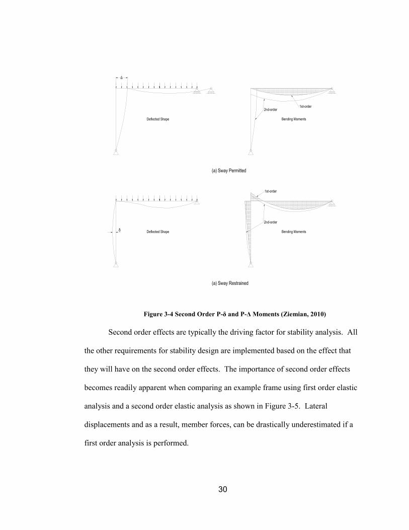
Figure 3-4 Second Order P-δ and P-Δ Moments (Ziemian, 2010)
Second order effects are typically the driving factor for stability analysis. All
the other requirements for stability design are implemented based on the effect that
they will have on the second order effects. The importance of second order effects
becomes readily apparent when comparing an example frame using first order elastic
analysis and a second order elastic analysis as shown in Figure 3-5. Lateral
displacements and as a result, member forces, can be drastically underestimated if a
first order analysis is performed.

31
Figure 3-5 Comparison of First Order Analysis to Second Order Analysis
(Adapted from Gerschwindner, 2009)
Second order analysis can be carried out per AISC 360-10 methods of either
rigorous second order analysis or the approximate second order analysis, both of
which are discussed in more detail in further sections.
The importance of second order effects on overall stability of structure can be
seen in various structural failures over the years. For example, in 1907, the Quebec
Bridge collapsed during construction due to failure of the compression chords of the

32
truss. In the weeks previous to the collapse, deflections in the chords was noticed and
reported but nothing was done and work continued until the eventual collapse of the
bridge. While many factors led to the failure of the bridge, one of the errors made in
the design of the bridge was in the design of the compression chords. The
compression chords were fabricated slightly curved for aesthetic reasons. However,
because this member curvature complicated the calculations, the members were
designed as straight members. Therefore, the actual second order effects were
increased and the buckling capacity was reduced when compared to the straight
member as designed. (Delatte, 2009) As can be seen from Figure 3-4 and 3-5, the
second order effects can increase both the displacement and moments to failure much
before Euler buckling load is ever reached. Figure 3-6 shows the Quebec Bridge
prior to collapse and Figure 3-7 shows the result of the failure.
Figure 3-6 Quebec Bridge Prior to Collapse (Canada, 1919)

33
Figure 3-7 Quebec Bridge after Failure (Canada, 1919)
Some general points concerning second order analysis made by Ziemian
(2010) are as follows:
1. Second order behavior can affect all components and internal member
forces within a structure.
2. Second order moments do not necessarily have the same distribution as
the first order moments and therefore the first order moments cannot be
simply amplified. LeMessurier (1977) and Kanchanalai and Lu (1979)
however give several practical applications where amplification of first
order moments to achieve an approximation of second order moments is
applicable.
34
3. All structures will experience both P-δ and P-Δ effects but the magnitude
of the effects will vary greatly between structures.
4. Linear superposition of effects cannot be used with second order analysis;
the response is non-linear.
3.4.3 Flexural, Shear and Axial Deformation
Second order effects are required in stability analysis as explained in the
previous section. Accurate deformation must be calculated because second order
effects are based on deformation to determine the amplified moments and forces.
The AISC 360-10 requires that flexural, shear and axial deformations be
considered in the design. Although flexural deformations will usually be the largest
contributor to overall structural deformation, axial and shear deformations should not
be ignored. Figure 3-8 shows a frame and the calculated deformations from flexural,
shear and axial. If shear and axial deformations were ignored in the design and
analysis, the amplifications of moments and forces from second order effects could be
underestimated and the structure could become unstable.

35
Figure 3-8 Deformation from Flexure, Shear and Axial (Adapted from Geschwindner,
2009)
3.4.4 Geometric Imperfections
Geometric imperfections refer to the out-of-straightness, out-of-plumbness,
material imperfections and fabrication imperfections. The maximum allowable
geometric imperfections are set by AISC Code of Standard Practice for Steel Building
and Bridges. The main geometric imperfections of concern in stability analysis are
member out-of-straightness and frame out-of-plumbness. Member out-of-straightness
is limited to L/1000, where L is the member length between brace or frame points.

36
Frame out-of-plumbness is limited to H/500, where H is the story height. (AISC 360-
10) (AISC 303-10)
Geometric imperfections cause eccentricities for axial loads in the structure
and members. These eccentricities need to be accounted for in stability analysis
because they can cause destabilizing effects and increased moments. Eccentricities
also increase the second order effects in the analysis of the structure. Maximum
tolerances specified by AISC Code of Standard Practice for Steel Buildings and
Bridges should be assumed for analysis unless actual imperfection values are known.
(AISC 360-10)
Columns are never perfectly straight and contain either member out-of-
straightness or general out-of-plumbness, therefore an initial eccentricity of the axial
load will be experienced. Figure 3-9 shows how the real column will behave with an
initial imperfection (yo). Nominal column capacity (Pn) will be reached well before
Euler Buckling load (Pcr). Second order effects are included in this graph of axial
load vs. deformation. Based on the presence of the initial displacement, moment will
develop and the column will typically yield based on flexure and compression while
the theoretical Euler buckling will never be reached.

37
Figure 3-9 Load vs. Deflection – Real Column Behavior with Initial Imperfections
3.4.5 Residual Stresses and Reduction in Stiffness
Residual stresses are internal stresses contained in a structural steel member.
There are several sources of residual stresses: (Salmon and Johnson, 2008)
1. Uneven cooling after hot rolling of the structural member. 2. Cold bending or cambering during fabrication.
3. Punching holes or cutting during fabrication.
4. Welding.
Uneven cooling and welding typically produce the largest residual stresses in
a member. Local welding for connections does produce residual stresses but the
presence of these stresses tend to be localized and are not considered in overall
column or beam design strength. Residual stress from uneven cooling happens when
the rolled shape is cooled at room temperature from the rolling temperatures. Certain

38
areas of the member will cool more rapidly than others. For example, the flange tips
of a wide flange shape are surrounded by air on three sides and cool more rapidly
than the material at the junction of the flange and web. As the flange tips cool, they
can contract freely because the other regions have yet to develop axial stiffness.
When the slower cooling sections begin to cool and contract, the axial stiffness from
the cooled regions restrains the contraction thus creating compression on the faster
cooling section and tension in the slower cooling sections. Figure 3-10 shows the
residual stresses typically seen in hot rolled wide flange shapes from uneven cooling.
(Vinnakota, 2006) (Huber and Beedle, 1954) (Yang et al., 1952)
Figure 3-10 Residual Stress Patterns in Hot Rolled Wide Flange Shapes
Welding of built up sections produces residual stresses as a result of the
localized heating applied during the welding. A built up wide flange shape will have

39
compression on the flange tips and middle of the web and tension around the junction
of the web and flange. (Vinnakota, 2006)
The presence of residual stresses results in a non-linear behavior of the stress
strain curve. The average yield stress of the section is reduced by the amount of
residual stress in the member. Therefore the section will start to yield before the
stress reaches the theoretical yield stress of a member with no residual stress. Linear
elastic behavior is experienced to the point of theoretical yield stress (Fy) minus the
residual stress (see Figure 3-11). After this point, non-linear behavior is experienced
and plasticity begins to spread through the section. (Salmon and Johnson, 2008)
Figure 3-11 Influence of Residual Stress on Average Stress-Strain Curve (Salmon and
Johnson, 2008)

40
Residual stresses need to be considered in stability analysis because of the
effect of general softening of the structure from the spread of plasticity through the
cross section causing reduced stiffness. The reduced stiffness increases deflections
and therefore increases the second order effects on the structure. (AISC 360-10)
Beam and column design strength is calculated based on empirical equations
which take into account the residual stress which is assumed to follow a Lehigh
pattern which is a linear variation across the flanges and uniform tension in the web.
The AISC 360-10 strength equations were developed and calibrated based on
research from Kanchanalai (1977) and ASCE Task Committee (1997). Figure 3-12
shows the idealized residual stresses for typical wide flange sections which follows
the Lehigh pattern. The residual stresses are assumed to be 0.3Fy in wide flange
shapes. (AISC 360-10) (Ziemian, 2010) (Deierlien and White, 1998)
Figure 3-12 Idealized Residual Stresses for Wide Flange Shape Members – Lehigh
Pattern (Adapted from Ziemian, 2010)

41
3.5 AISC Methods of Stability Analysis
As discussed before, AISC 360-10 states that any method that considers the
influence of second-order effects, flexural, shear and axial deformation, geometric
imperfections, and member stiffness reduction due to residual stresses on the stability
of the structure and its elements is permitted.
Various types of methods of have been developed and AISC 360-10 detailed
the requirements for a few of these methods. Each method listed, does in some way,
address all the various requirements specified by AISC 360-10. All methods listed in
AISC 360-10, excluding the first order analysis method, require a second order
analysis. Table 2-2 from AISC 360-10 provides a summary of requirements and
limitations of each of the methods. AISC 360-10 allows two types of second order
analysis; Approximate Second Order Analysis and Rigorous Second Order Analysis.
Both methods of second order analysis either accurately account for or
approximate geometric nonlinear behavior. In reality, geometric nonlinear behavior
is only one of the nonlinear types of behavior that should be considered in design.
Material nonlinear behavior (inelastic analysis) caused by reduction in stiffness
should also be considered in design. Figure 3-13 shows the results from various types
of analyses.

42
Figure 3-13 Load vs. Deflection – Comparison of Analysis Types (Adapted from White and
Hajjar, 1991)
While software is available that performs a true second order inelastic
analysis, it is very computationally expensive, and therefore other measures must be
considered in analysis and design. AISC 360-10 strength equations are typically
based on the results from a second order elastic analysis. The AISC LRFD general
approach for strength and stability can be represented by the following equation:
Σγi*Qi ≤ ΦRn

43
The left hand side of the formula represents the effects of factored loads on a
structural member, connection and the right side represents the design resistance or
design strength of the specified element with:
Qi = internal forces created by applied load
Rn = Nominal member or connection strength
γi = factor to account for variability in load (load factor)
Φ= factor to account for variability in resistance (strength reduction factor)
Geometric nonlinear behavior can be accounted for using a second order
elastic analysis (left side of the equation). These load effects are then compared to
resistance based on material and geometric inelasticity (right side of the equation).
(Yura el al., 1996) As Figure 3-13 shows, a direct comparison of load effects from
second order elastic analysis and member resistance is not compatible because the
inelastic material deflections are not considered in an elastic second order analysis.
Therefore AISC 360-10 design equations should be calibrated for the results of an
elastic second order analysis or the effects of material inelasticity must be accounted
for in the elastic second order analysis. (Ziemian, 2010) This can be accomplished
through various methods discussed in more detail in further sections.
3.5.1 Rigorous Second Order Elastic Analysis
To fully capture the second order effects as described in previous sections,
non-linear geometric behavior should be accurately calculated. With the constant

44
increase of computational capabilities, rigorous second order analysis is becoming
much more common in design practice. It should be noted that the AISC 360-10
definition of rigorous second order analysis is typically not meant to represent a true
non-linear second order analysis but will still produce results that accurately calculate
the second order effects. Many methods can be used for analysis but the general form
is usually expressed as: (Ziemian, 2010)
{dF}-{dR} = K{dΔ}
With:
{dF} = Vector of incremental applied nodal forces
{dR} = Vector of unbalanced nodal forces, difference between current internal
forces and applied loads
K = Stiffness matrix
{dΔ} = Vector of incremental nodal displacements and rotations
Most solutions use an iterative approach for solving for second order effects.
The unbalanced forces are calculated based on the deformed geometry at the end of
each iteration and used as the basis for the next iteration. Iterations can be performed
until the unbalanced force vector is determined to be negligible. Figure 3-14 shows a
method commonly referred to as the Newton-Raphson incremental – iterative
solution.

45
Figure 3-14 Visual Representation of Incremental – Iterative Solution Procedure (Adapted from
Ziemian, 2010)
Additional methods based on the Newton-Raphson incremental-iterative
solution have been developed based on the limitation imposed by the use of this
solution. McQuire et al. (2000) and Chen and Lui (1991) have provided general
overview of additional methods.
A variation of these methods that can be used by STAAD.Pro V8i is referred
to as the Lagrangian procedure. This procedure revises the stiffness matrix, K, to
take the following form:
[K] = [Ke] + [Kg]
46
With Ke being the standard linear elastic stiffness matrix and Kg being the geometric
stiffness matrix. This method recognizes that as the structure deforms the stiffness
associated with the member forces is changed at each increment of the solutions.
This leads to more accurate results and the ability to use this type of solution for
dynamic analyses because the method accounts for change in the natural period due
to second order effects and the stiffening of the structure. (Galambos, 1998) This
procedure is given in more detail by Crisfield (1991), Yang and Quo (1994) and
Bathe (1996). STAAD Technical Manual (2007) also gives details of how this
method is applied for analysis.
3.5.2 Approximate Second Order Elastic Analysis
In lieu of a rigorous second order elastic analysis which is iterative and can
demand extensive computational effort, approximate second order analysis methods
have been developed over the years to potentially simplify analysis. Rutenberg
(1981, 1982), White et al (2007a,b) and LeMessurier (1976, 1977) have each
developed approximate methods of analysis to either simplify analysis in computer
applications or simplify hand calculations. (Ziemian, 2010)
The AISC 360-10 method of approximate second order analysis uses
amplification factors B1 and B2 to account for P-δ and P-Δ effects, respectively. See
AISC 360-10 Appendix 8 for the procedure.

47
Because this approximate second order analysis is typically used for hand
calculations of frame analysis, no additional discussion will ensue based on the
assumption that the engineer has access to software capable of a rigorous second
order analysis.
3.5.3 Direct Analysis Method
Introduced in AISC 360-05, the direct analysis method represents a
fundamentally new alternative to traditional stability analysis methods. (Griffis and
White, 2010) The most significant development addressed in this method is that
column strength can be based on the unbraced length of the member therefore
eliminating the need to calculate the effective length of the member (K may be taken
as 1 for all members). (Ziemian, 2010)
While all the requirements for AISC stability analysis are covered with this
method, slight variations in each requirement are allowed and discussed in further
detail. One major advantage of the direct analysis method is that it has been
developed and verified for application to all types of structural systems and therefore
has no limitations for use. (Maleck and White, 2003)
Accurate second order analysis is the cornerstone of the direct analysis
method. As previously discussed, two types of second order analysis are allowed by
AISC 360-10, rigorous second order analysis and approximate second order analysis.
As with all AISC 360-10 methods that use second order analysis results, the direct

48
analysis method is built around the assumption of LRFD loads and therefore if ASD
loads are to be used in analysis, they must be multiplied by 1.6 before second order
analysis is completed because of the nonlinearity of second order effects. (AISC 360-
10) (Nair, 2009)
Flexural, shear and axial deformations need to be considered in analysis. As
previously discuss, accurate deformations are needed for calculation of second order
effects. However, in discussion of shear and axial deformation AISC 360-10
explicitly uses the word “consider” instead of “include”. This allows the engineer to
ignore certain deformations based on the type of structural system. For example, the
shear deformations could feasibly be neglected in a low rise moment frame and
produce results with an error of less than 3%. High rise moment frame systems on
the other hand, could produce much higher errors if shear deformations were to be
neglected. (AISC 360-10) Most modern analysis software is capable of calculating
accurate flexure, shear and axial deformations, and very little effort by the engineer is
required to achieve the most accurate results available by the software.
The direct analysis method is calibrated on the assumption that geometric
imperfections are equal to the maximum material, fabrication and erection tolerances
permitted by the Code of Standard Practice for Steel Buildings and Bridges (AISC
303-10). Geometric imperfection may be accounted for by two methods; direct
modeling of imperfections or notional loads. (AISC 360-10) Direct modeling of
imperfections can become quite tedious because as a minimum, four models must be
49
developed, each with the deflection in one of the four principle directions with the
additional member out of straightness modeled corresponding to the worst case
direction. Notional loads are defined as horizontal forces added to the structure to
account for the effects of geometric imperfections. (Ericksen, 2011) For the direct
analysis method the magnitude of notional loads applied to the structure is 0.2% of
the total factored gravity load at each story.
Ni = 0.002αYi
With:
α = 1.0 (LRFD); 1.6 (ASD)
Ni = Notional lateral load applied at level i, kips
Yi = Gravity load applied at level i from the LRFD or ASD load
combinations as applicable, kips
It can be see that 0.2% of gravity loads is appropriately selected as 1/500
which also corresponds to the maximum out-of-plumbness for columns from AISC
303-10. Analysis will show that either applying a notional load of 0.2% or directly
modeling out-of-plumbness will produce similar results. (Malek and White, 1998)
Member out-of-plumbness is accounted for by notional loads, but member out-of-
straightness still needs to be considered in design. AISC 360-10 has developed the
column strength equations based on maximum out-of-straightness tolerances.
(Ziemian, 2010) (White et al., 2006)
50
For the direct analysis method, notional loads should be applied in
combination with all gravity and lateral load combinations to create the worst effects.
AISC 360-10 does however, allow notional loads to be applied only to gravity load
combinations as long as the ratio of second order to first order drifts does not exceed
1.5 using the unreduced elastic stiffness or 1.7 if the reduced elastic stiffness is used
in analysis. The errors seen by this simplification are relatively small as long as the
ratio of drifts remains below the specified limits. (AISC 360-10)
Reduction in stiffness of the structure is caused by partial yielding of
members. This yielding is further accentuated by residual stresses. The direct
analysis method specifies reduced stiffnesses of EI* and EA* with:
EI* = 0.8τbEI
EA* = 0.8EA
The reduced stiffness factor of 0.8 is applied for two reasons. The first and
most readily apparent is the reduction in stiffness in intermediate and stocky
members, namely columns, due to inelastic softening of members before they reach
their design strength. The second reason relates to slender members that are governed
by elastic stability. 0.8 is roughly equivalent to the product of Φ= 0.9 and the factor
0.877. These factors are used in development of the AISC column curve (AISC 360-
10 Eqn. E3-3) which is modified by the above factors for slender elements to account
for member out-of-straightness. (Ziemian, 2010) (AISC 360-10)

51
The τb value is an adjustment factor to account for additional reduction in
stiffness in cases where high axial stresses are present which can reduce the bending
stiffness of the member. (AISC 360-10)
τb = 1.0 when αPr/Py ≤ 0.5
τb = 4(αPr/Py)[1-( αPr/Py)] when αPr/Py ≥ 0.5
where:
α = 1.0 (LRFD); 1.6 (ASD)
Pr = Required axial compressive strength using LRFD or ASD load
combinations.
Py = Axial Yield strength (Ag*Fy)
AISC 360-10 does allow τb = 1.0 for all cases if the notional load is increased
by 0.1%Yi. This additional notional load is meant to increase the lateral deformation
to envelope the effects caused by reduction in stiffness in high axial loaded members.
However, Powell notes that this method does not appear to be logical because
notional loads are meant to account for initial out of plumbness and not for reduction
in stiffness (Powell, 2010). Figure 3-15 shows a graphical representation of the effect
of τb on the reduction in stiffness.

52
Figure 3-15 Reduced Modulus Relationship (Powell, 2010)
3.5.4 Effective Length Method
In recent years, the traditional method for stability analysis has been the
effective length method. In general, the effective length method calculates the
nominal column buckling resistance using an effective length (KL) and the load
effects are calculated based on either a rigorous or approximate second order analysis.
(Ziemian, 2010)
As with the direct analysis method, the effective length is built around
determining accurate second order effects. This can be done by either a rigorous
second order analysis or by an approximate second order analysis. (AISC 360-10)
Both methods of second order analysis are based on the assumption that flexural,
shear and axial deformations are considered in calculations of second order effects.

53
Prior to AISC 360-05, there were few limitations on applications of the
effective length method. Several studies by Deierlein et al. (2002), Maleck and White
(2003), and Surovek-Maleck and White (2004a and 2004b) have shown that use of
the effective length method could produce significantly unconservative results in
certain types of framing systems. Therefore AISC 360-05 imposed additional
requirements and limitations.
1. Notional loads need to be included in gravity only load combinations to
account for member out-of-plumbness.
2. The ratio of second order drift to first order drift or B2 is limited to 1.5.
Geometric imperfections are covered by applications of notional loads or
direct modeling of imperfections for analysis. Notional loads are applied in the same
manner as described with the direct analysis method with: (AISC 360-10)
Ni = 0.002αYi
However, based on the limitation of the ratio of second order drift to first
order drift or B2, by definition, notional loads need only be applied to gravity load
combinations.
One of the main components of the effective length method is the calculation
of the effective length factor K. The most common method for determining K is
through the use of the alignment charts found in the commentary for Appendix 7 in
AISC 360-10 which can be seen in Figures 3-16 and 3-17.

54
Figure 3-16 Alignment Chart – Sidesway Inhibited (Braced Frame) (AISC 360-10)

55
Figure 3-17 Alignment Chart – Sidesway Uninhibited (Moment Frame) (AISC 360-10)
The alignment charts were developed based on the following assumptions:
1. Behavior is purely elastic.
2. All members have constant cross section.
3. All joints are rigid.
4. For columns in frames with sidesway inhibited, rotations at opposite ends
of the restraining beams are equal in magnitude and opposite in direction,
producing single curvature bending.

56
5. For columns in frames with sidesway uninhibited, rotation at opposite
ends of the restraining beams are equal in magnitude and direction,
producing reverse curvature bending.
6. The stiffness of parameter L√(P/EI) of all columns is equal.
7. Joint restraint is distributed to the column above and below the joint in
proportion to EI/L for the two columns.
8. All columns buckle simultaneously
9. No significant axial compression force exists in the girders.
The assumptions listed above, seldom if ever are seen in a real structure and
therefore additional methods of determining K have been developed.
Geschwindner(2002) and ASCE Task Committee (1997) have provided an overview
of the various methods for determining accurate values of K. In addition to methods
listed in AISC 360-10, Yura (1971) and LeMessurier (1995) presented various
approaches for calculation of the effect length factor K. Folse and Nowak (1995) also
presented examples that included the effect of leaning columns.
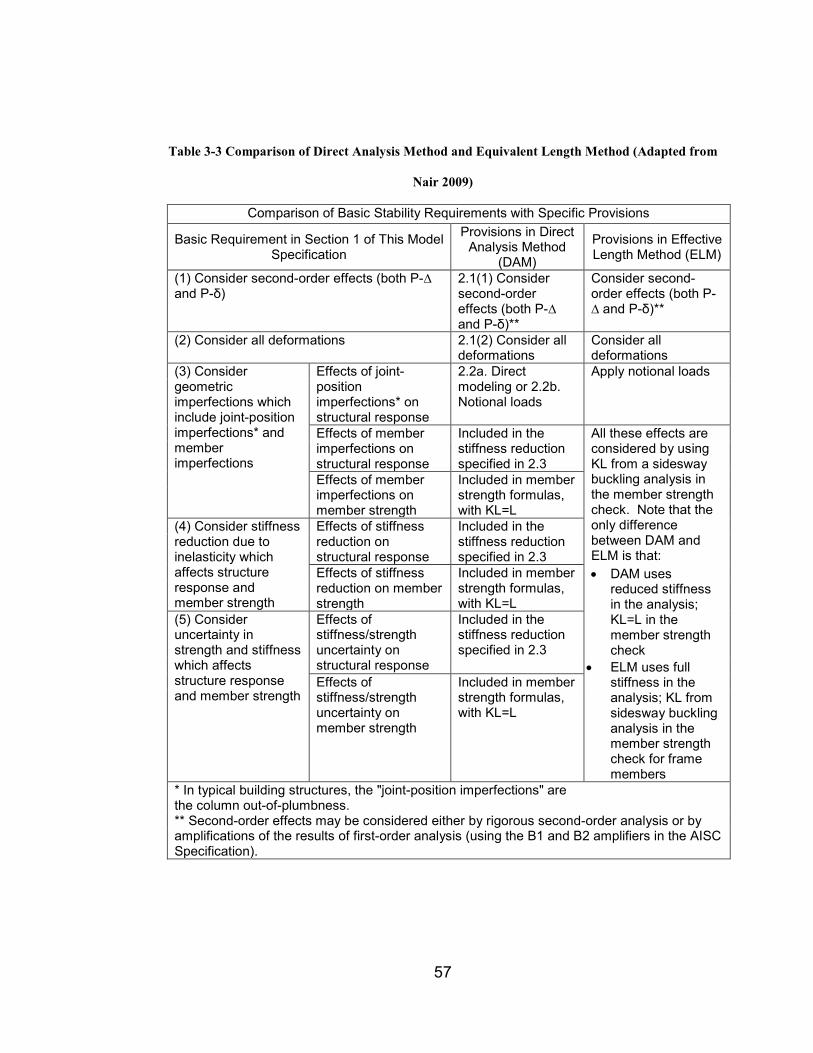
The table below gives a comparison of the equivalent length method and the
direct analysis method and describes how each method addresses the stability analysis
requirements of AISC 360-10.
57
Table 3-3 Comparison of Direct Analysis Method and Equivalent Length Method (Adapted from
Nair 2009)
Comparison of Basic Stability Requirements with Specific Provisions
Basic Requirement in Section 1 of This Model Specification
Provisions in Direct Analysis Method
(DAM)
Provisions in Effective Length Method (ELM)
(1) Consider second-order effects (both P-∆ and P-δ)
2.1(1) Consider second-order effects (both P-∆ and P-δ)**
Consider second-order effects (both P-∆ and P-δ)**
(2) Consider all deformations 2.1(2) Consider all deformations
Consider all deformations
(3) Consider geometric imperfections which include joint-position imperfections* and member imperfections
Effects of joint-position imperfections* on structural response
2.2a. Direct modeling or 2.2b. Notional loads
Apply notional loads
Effects of member imperfections on structural response
Included in the stiffness reduction specified in 2.3
All these effects are considered by using KL from a sidesway buckling analysis in the member strength check. Note that the only difference between DAM and ELM is that:
Effects of member imperfections on member strength
Included in member strength formulas, with KL=L
(4) Consider stiffness reduction due to inelasticity which affects structure response and member strength
Effects of stiffness reduction on structural response
Included in the stiffness reduction specified in 2.3
Effects of stiffness reduction on member strength
Included in member strength formulas, with KL=L
• DAM uses reduced stiffness in the analysis; KL=L in the member strength check
(5) Consider uncertainty in strength and stiffness which affects structure response and member strength
Effects of stiffness/strength uncertainty on structural response
Included in the stiffness reduction specified in 2.3
• ELM uses full stiffness in the analysis; KL from sidesway buckling analysis in the member strength check for frame members
Effects of stiffness/strength uncertainty on member strength
Included in member strength formulas, with KL=L
* In typical building structures, the "joint-position imperfections" are the column out-of-plumbness. ** Second-order effects may be considered either by rigorous second-order analysis or by amplifications of the results of first-order analysis (using the B1 and B2 amplifiers in the AISC Specification).

58
3.5.5 First Order Method
The first order analysis method is a simplified method derived from the direct
analysis method. (Kuchenbecker et al., 2004) The main benefit of this method is that
only a first order analysis is required. In addition, because it is based on the direct
analysis method, K can be set at 1 for all cases. (AISC 360-10)
The main simplification in this method comes from the assumption that the
ratio of second order drift to first order drift or B2, is assumed to be equal to1.5.
From this assumption, equivalent notional lateral loads can be back calculated which
simulate the effects of second order effects as well as reduction in stiffness due to
partial yielding which are both accounted for using the direct analysis method.
(Ziemian, 2010)
The simplification and assumptions which are made in development of the
first order method lead to limitations on use of this method. The ratio of second order
drift to first order drift or B2 is assumed to be 1.5, which sets the maximum allowed
value for application of this method. The stiffness reduction of 0.8 was also assumed
in calculations of additional notion loads and therefore, based on the previous
discussion of the reduction in stiffness, αPr/Py ≤ 0.5 must be maintained for the 0.8
reduction in stiffness to remain true.
The notional load Ni for the first order analysis method is defined as:
(Kuchenbecker et al., 2004)
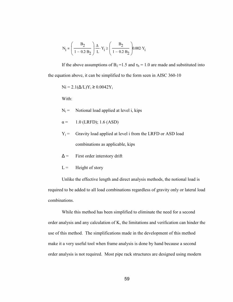
59
NiB2
1 0.2 B2⋅−
∆
L⋅ Yi⋅
B21 0.2 B2⋅−
0.002 Yi⋅≥
If the above assumptions of B2 =1.5 and τb = 1.0 are made and substituted into
the equation above, it can be simplified to the form seen in AISC 360-10
Ni = 2.1(Δ/L)Yi ≥ 0.0042Yi
With:
Ni = Notional load applied at level i, kips
α = 1.0 (LRFD); 1.6 (ASD)
Yi = Gravity load applied at level i from the LRFD or ASD load
combinations as applicable, kips
Δ = First order interstory drift
L = Height of story
Unlike the effective length and direct analysis methods, the notional load is
required to be added to all load combinations regardless of gravity only or lateral load
combinations.
While this method has been simplified to eliminate the need for a second
order analysis and any calculation of K, the limitations and verification can hinder the
use of this method. The simplifications made in the development of this method
make it a very useful tool when frame analysis is done by hand because a second
order analysis is not required. Most pipe rack structures are designed using modern

60
analysis software which is capable of performing a second order analysis, therefore
the first order method will likely see limited use for pipe rack applications.
61
4. Research Plan
A literature review was first conducted to gather and review the available
information pertaining to the design and engineering of pipe rack structures for use in
industrial facilities. The industry is constantly evolving, and the most current
literature discussing the design and engineering of pipe racks was targeted for review.
Next, a literature review was conducted to gather and review the available
information pertaining to AISC stability analysis. Literature that described the
various methods used by both AISC 360-05 and AISC 360-10 were the focus of the
review. The direct analysis method literature was of particular interest as it was a
relatively new development in regards to stability analysis.
A general plan for the research that was conducted is presented here and is
described as follows:
1. Use Benchmark Problems from AISC 360-10 to test the second order analysis
capabilities of STAAD and report on the validity of the STAAD approach.
2. Describe in detail a typical pipe rack to be used for comparison of the
methods.
3. Develop general loads and load combinations for use in the analysis models.

62
4. Develop a general STAAD.Pro V8i model that can be used for analysis of the
Equivalent Length Method, Direct Analysis Method and First Order Method
with input from [2] and [3].
5. Complete a first order analysis of the pipe rack structure developed in [4] for
use in calculation of the Δ2/Δ1 ratio as well as for use in the First Order
Method and discuss the results and validity of the method based on AISC
limitations
6. Optimize strength only design of test pipe rack structure developed in [4]
using Equivalent Length Method and determine validity of method for current
structure based on AISC limitations
7. Optimize the strength only design of the test pipe rack structure developed in
[4] using the Direct Analysis Method and compare the results to the
Equivalent Length Method.
8. Use the models developed in [6] and [7] and vary member sizes and base
fixity based on the serviceability limits and compare the results.
9. Compare the results of [5 to 8].

63
5. Member Design
The available strength of members should be calculated in accordance with
the provisions of AISC 360-10 Chapters D, E, F, G, H, I, J and K. These chapters
should be used regardless of the method of stability analysis chosen. Column design
can become a major point of focus during stability analysis based on several factors.
The effective length factor for column design can become complex for even simple
structures when using the effective length method of stability analysis. Columns
typically experience combined flexural, shear and axial load and the interaction
between each stress must be investigated.
The two methods of stability analysis; effective length and direct analysis, as
expected, produce varying load effects. A design example is shown in Figure 5-1
showing a simple cantilever W10X60 column bent about the strong axis with an axial
load P and the horizontal load H = 10%P. The column is assumed to be supported
out of plane resulting in only strong axis buckling. Stability analyses using both the
equivalent length method and the direct analysis method were performed. A linear
elastic analysis was performed as well to establish a first order baseline for
comparison. STAAD.Pro V8i was used for both methods of stability analysis while
hand calculations were done to compute the linear elastic forces.

64
Figure 5-1 Simple Cantilever Design Example
The cantilever column was then checked against the code specified available
strength. The column in this example will experience both axial and flexural loads,
therefore AISC 360-10 Chapter H will be used to determine the available strength.
A simple cantilever column was chosen to simplify the selection of the effect
length factor K. The theoretical value of K for a fixed base cantilever column is 2.
Therefore the effective length of the column used for the determining the available
strength using the effective length method will be 30 ft.
65
Figure 5-2 shows a graph of axial load vs. moment for the simple cantilever
example. AISC 360-10 equations H1-1a and H1-1b are included on the graph for
design purposes. When comparing methods of analysis, with the linear elastic
method as a baseline, the differences are readily apparent. As expected, the linear
elastic method produces linear results of axial load vs. moment. Based on the theory
of stability analysis, the linear elastic method is expected to produce results that
overestimate the axial resistance and underestimate the moment demand. When
comparing the results of both the effective length and direct analysis methods, the
resistance based on AISC 360-10 equations H1-1a and H1-1b must be adjusted based
on the effective length factor K. This will affect the axial resistance of the column
section. The direct analysis method assumes that K = 1 and the effective length
method assumes that K = 2 for a fixed base cantilever column. This changes the
“anchor point” interaction equations.

66
0
100
200
300
400
500
600
700
800
900
0 50 100 150 200 250 300
M (ft-kips)
P (k
ips) Direct Analysis Method
(Demand)
Effective Length Method(Demand)
Linear Elastic Method(Demand)
ΦcPn K=1
ΦcPn KL
AISC Eqn. H1-1a(Resistance)
AISC Eqn. H1-1b(Resistance)
Figure 5-2 Simple Cantilever Design Example Results
One of the main differences in results between the effective length method
and the direct analysis method is the moment demand. The axial load resistance is
comparable between the two methods but the moment demands can differ
significantly. The column capacity is adjusted between the methods based on the
effective length factor which calibrates the axial capacity. The difference in moment
demand is due to the reduction in stiffness used in the direct analysis which increases
deformations which in turn increases eccentricities and therefore moment demand is
increased.

67
Based on the results of this design example, several observations can be made:
(AISC 360-10)
1. Accurate calculations of the effective length factor, K, are critical to
achieving accurate results using the effective length method.
2. The moment demand is underestimated when using the effective length
method. This can significantly affect the design loads for beams and
connections which provide rotational resistance for the column.
68
6. Pipe Rack Analysis
6.1 Generalized Pipe Rack
A typical pipe rack will be developed and used for comparison purposes for
this thesis. The typical pipe rack was chosen and modeled based on idealized
conditions. A width of 15 feet was chosen to allow one-way traffic along the pipe
rack corridor. The height of the first level of the pipe rack was set at 20 feet to
provide sufficient height clearance along the access corridor.
The overall length of the pipe rack was set at 100 feet. Longer pipe rack
sections are typically broken into shorter segments (100 to 200 feet) with each shorter
segment separated by expansion joints to allow thermal expansion or contraction
between segments. One of the lengthwise central bays of each segment is typically
braced in the longitudinal direction. This allows the length of the pipe rack to expand
and contract about a central braced bay and reduces thermally induced loads cause
from restraint of thermal movement. If each end of the segment were to consist of a
braced frame, the length of the pipe rack would essentially be locked in place and
higher thermally induced loads would be seen.
Moment frames are typically spaced at 15-20 feet. This spacing is typically
chosen based on the maximum allowable spans for the pipes or cable trays being
supported. This spacing can vary based on the estimated size and allowable
deflection limits of the pipe being supported

69
Longitudinal struts are usually offset from the beams used to support the
pipes. Levels of the pipe rack are assumed to be fully loaded with pipe, and when the
pipes need to exit the rack to the side to connect to equipment, a flat turn cannot be
used as this would clash with the other pipes on the same level. The pipe is typically
routed to turn either up or down and then out of the rack at the level of the
longitudinal struts where the pipe can be supported on the longitudinal struts before
exiting the rack.
To allow room for pipes to enter and exit the pipe rack, a spacing of 5 feet
between levels is typically used. If the pipe rack carries larger pipes, additional room
may be required between levels. This spacing should be determine with the help of
the piping engineer on the project. Spacing between pipe rack levels of 5 feet will be
used in this thesis.
Figure 6-1 shows an isometric view of the typical pipe rack that will be used
for analysis and comparison of stability analysis methods. While this is not
representative of all pipe racks, it will still provide a useful basis for comparison
purposes in pipe rack structures.

70
Figure 6-1 Isometric View of Typical Pipe Rack Used for Analysis
To simplify the design and analysis, a typical moment frame will be selected
and isolated for analysis and design. Figure 6-2 shows an elevation view of a typical
moment frame.

71
Figure 6-2 Section View of Moment Frame in Typical Pipe Rack
Out-of-plane supports were added at the locations of longitudinal struts which
will restrain any movement in and out of the page (see Figure 6-1). Longitudinal
struts all tie into the braced bay, therefore relatively small deflections will be
experienced in the weak axis of the columns and the restraint of any movement in this
direction is a reasonable assumption.
Based on initial calculations that compare the results of the isolated moment
frame and the entire pipe rack segment, relatively small differences were seen.
Because the braced bay supports any longitudinal loading, relatively very little weak
axis column moment or longitudinal deflection occurs that would affect the design of

72
the columns or beams that are part of the moment frame. Ratios of demand to
capacity showed errors of less than 5% on member design when using the single
frame compared to the full pipe rack structure. Therefore, analysis of a single
moment frame will be used to simplify calculations. The focus of this thesis will
mainly be on the analysis of the moment frame; the braced frame will not be
considered in analysis and design.
In actual design, engineering judgment should be used to determine if the
analysis of a single frame simplification can be made. In many cases, pipe racks are
not symmetric and loading can vary from frame to frame and the overall structure
should be analyzed as a whole to determine the load effects. Bracing systems should
also be designed to resist the longitudinal loads of the entire segment and therefore
modeling of the entire pipe rack segment may be required to determine load path and
design loads for struts and braces.
6.2 Pipe Rack Loading
The pipe rack used for analysis and comparison of methods will have
consistent loading between methods to limit the number of variables. In general,
loads in the longitudinal direction will not be considered in design and comparison
because the focus of analysis will be on the behavior and performance of the moment
frame. Therefore, wind and seismic loading, will only be considered in the transverse
directions.

73
In practice, engineering judgment should be used in determining all applicable
loads. The following discussion is meant to define loads only for analysis and
comparison of the stability analysis and therefore certain simplifications are made to
facilitate analysis but still provide results that are typical of pipe racks.
All loads are developed based on the assumption that the pipe rack is
considered an Occupancy Category III. (PIP STC01015) This will affect the
importance factor used for development of wind and seismic loading.
The primary load cases, which were defined previously, were chosen
according to PIP STC01015. Additional primary load cases may be required based
on the requirements of AISC 360-10 for notional loads. Loads are developed based
in input from ASCE 7-05. While ASCE 7-10 is available, PIP STC01015 has not
been updated to reflect the changes made by ASCE 7-10.
The first primary load case defined was the dead load of the structure (Ds).
This is considered as the self-weight of the steel. For design, an additional 10% of
the self-weight was added to account for fabrication tolerances and additional
materials used for connections. No other loads were assumed at this time for the dead
load of the structure.
The operating dead load as discussed previously is typically applied at 40 psf,
which assumes a fully loaded level with 8 inch pipes full of water spaced at 15
inches. The representative pipe rack will use 40 psf applied over the entire tributary

74
area of the pipe rack. The spacing of the moment frames was chosen as 20 feet,
therefore the uniform load applied at each level of the pipe rack is 800 pounds per
foot. This load can be seen in Figure 6-3.
Figure 6-3 Section View of Moment Frame - Operating Dead Load
The empty dead load of the pipe can be taken as 60% of the operating dead
load unless further information is known. This calculates to 480 pounds per foot.
The empty dead load of the pipe is applied in a similar fashion as seen in Figure 6-3.
Test dead load is the weight of the pipe plus the weight of the test medium.
This type of loading will typically control when the majority of the pipes in the pipe

75
rack are filled with gas or steam during operation. Hydro-testing is typically done to
test the piping prior to startup. Pipes were assumed to be full of water for the
operating load, therefore for this analysis, the test dead load is equivalent to the
operating dead load and the load is exactly as seen in Figure 6-3.
The erection dead load can account for any additional loads or reduction in
loads due to erection activities. This is typically used for any equipment and is based
on the fabricated weight. For piping, the erection dead load and the empty dead load
are typically the same. Therefore, the erection dead load case is not defined at this
time and if required in load combinations, the empty dead load can be used in place
of the erection dead load.
Pipe anchor and pipe friction loads are typically based on actual loading
conditions of pipes located in the pipe rack. However, without final pipe loading, an
estimate of pipe loads must be made. Friction forces can be estimated based on the
coefficient of friction between the pipe shoe and support beam. This coefficient of
friction is usually assumed to be 0.4. Application of 40% of the operating dead load
tends to be extremely conservative. Friction loads are cause by expansion and
contraction of pipes. Based on the expansion and contraction of pipes, friction loads
are typically seen in the longitudinal direction of the pipe rack. Because it is highly
unlikely that all pipes will expand and contract simultaneously and some pipes may
contract while others expand, a more realistic value of 10% of operating dead load
will be applied in the longitudinal direction. Friction loads are applied to the pipe

76
rack because the location of the loading could cause additional second order effects in
the beams in the moment frames.
While friction loads and anchor loads are typically only seen in the
longitudinal direction of the pipe rack, cases where anchor loads are seen in the
transverse direction could happen. Therefore apply 5% of the operating dead load as
a conservative estimate for the representative pipe rack. Figure 6-4 shows the
application of pipe anchor loads. In practice, local members should be checked for
pipe anchor loads and friction loads as the individual member design may be
controlled by high anchor loads.

77
Figure 6-4 Section View of Moment Frame - Pipe Anchor Load
Self-straining thermal loads will not be considered in design. A design ΔT of
0 degrees Fahrenheit will be applied to all members. Thermal loading can cause
problems if members are restrained from expansion or contraction. As the 2-D
moment frame has very little resistance for thermal movements, thermal loads will
not be considered in design of the representative model. Additional thermal
considerations could be considered but are outside the scope of this thesis.

78
Live load is typically only applicable to platforms or walkways required for
access, therefore live load will not be applied based on the assumption of no access
platforms or walkways on the simplified pipe rack.
Similarly, snow load typically will not control the design and therefore will
not be considered in the simplified analysis model. (PIP STC01015)
Wind load is applied consistent with ASCE 7-05 principles. For comparison
purposes, a 3 second gust wind velocity was assumed to be 100 miles per hour which
should cover a larger majority of sites. Additional information given by ASCE Wind
Loads for Petrochemical Facilities is included in wind load development. The
following velocity pressures at specified heights was developed according to ASCE
7-05. Table 6-1 shows velocity pressures for cable tray and structural members and
Table 6-2 shows velocity pressures for pipes.
Table 6-1 Velocity pressures for cable tray and structural members
Cable Tray and Structural Members
Height qz (ft) (psf)
0-15 21.270 20 22.522 25 23.523 30 24.524 40 26.025

79
Table 6-2 Velocity pressures for pipe
Pipe Height qz
(ft) (psf) 0-15 23.77 20 25.17 25 26.29 30 27.41 40 29.09
The design wind force for structural members varies based on the projected
area perpendicular to the wind direction and therefore will vary based on member
size. In the case where the wind is parallel to the strong axis, the flange width defines
the projected area. Structural shapes are assumed to have an average coefficient of
drag (Cf) of 2.0 for all wind directions. Pipes were assumed to have a coefficient of
drag (Cf) of 0.8 for wind perpendicular to pipe.
The design wind force for pipe is calculated based on the assumption of the
largest pipe being 8 inches. 10% of the pipe rack width is added to the pipe added to
the largest pipe diameter and multiplied by the bay spacing to determine a tributary
area. (ASCE, 2011) To simplify the design, the total force from the pipes on each
level is evenly divided and applied to each joint. This load could also be applied as a
uniform load across the entire length of the beam. Table 6-3 shows the resulting joint
loads resulting from wind loading on pipes.

80
Table 6-3 Resultant design wind force from pipe
Height F F/2 (ft) (lbs) (lbs)
0-15 701 350 20 742 371 25 775 387 30 808 404 40 857 429
Figure 6-5 shows the application of wind load for the typical pipe rack. The
resultant load from pipe wind load is evenly distributed at the end joints. The design
wind force shown for structural members is based on a column size of W10X33 with
a flange width of 8 inches. This design wind force will vary based on column size but
will provide a basis for application of wind load.

81
Figure 6-5 Section View of Moment Frame - Wind Load
Seismic loading is based on specific site information. The ASCE 7-05
Equivalent Lateral Force Procedure will be used for seismic loading. Because this is
a representative model, estimates on seismic loading will be made to simulate the
general seismic load effects. The pipe rack is assumed be in located in site class C or
below. An R value of 3 is chosen to simplify detailing requirements. The assumed
seismic response coefficient, Cs, will be 0.15. While the natural period of the
structure will depend on member size and base support conditions, the natural period

82
will be assumed to be greater than 0.5 seconds which is used to determine the vertical
distribution.
Based on the above assumptions, seismic forces can be developed and applied
to the structure. The effective seismic mass is based on previously discussed dead
loads, both operating and empty dead loads. Table 6-4 shows the applied operating
seismic load applied at each level of the pipe rack while Table 6-5 shows the applied
empty seismic load. The lateral force at each level will be evenly divided and applied
to each joint. See Figure 6-6 for operating seismic loading. Empty seismic loading is
similar to loading shown in Figure 6-6
Table 6-4 Lateral seismic forces - operating
Fx (lbs) Fx/2 (lbs) Level 1 950 475 Level 2 1450 725 Level 3 2100 1050 Level 4 2850 1425
Table 6-5 Lateral seismic forces - empty
Fx (lbs) Fx/2 (lbs) Level 1 600 300 Level 2 900 450 Level 3 1250 625 Level 4 1700 850

83
Figure 6-6 Section View of Moment Frame Lateral Seismic Load – Operating Seismic
6.3 Pipe Rack Load Combinations
Load combinations used for the representative model were developed from the
PIP STC01015 load combinations as discussed in previous sections. As the model
was simplified to isolate a moment resisting frame and study the results from
essentially a 2-D analysis, loading in the transverse direction was the focus for

84
developing load combinations. Because lateral loads are typically reversible, this can
create hundreds of load combinations if all load directions are considered. Transverse
only loading simplified the loading and resulted in fewer load combinations. In the
cases where notional loads are required, the notional load was considered to act only
in the direction causing the worst effect on stability which is typically in the same
direction as the lateral load.
Two sets of load combinations were developed for analysis and comparison
purposes. The first set applied notional loads to only the gravity only load
combinations. This set of load combinations is used for analysis using both the
effective length and direct analysis methods. The first set of load combinations can
only be used for the direct analysis when the ratio of second order to first order drift
is less than 1.7 if using reduced stiffness or 1.5 using unreduced stiffness per AISC
360-10.
The second set of load combinations applies the notional loads as additive in
all load combinations to create the worst effect on stability. The second set of load
combinations was developed for analysis using the direct analysis method where the
ratio of second order to first order drift is greater than 1.7 if using reduced stiffness or
1.5 using unreduced stiffness. The second set of load combinations can also be used
for the first order method where the notional loads are additive for all load
combinations. Although the magnitude of notional loads varies between the direct
analysis and first order method, the notional loads can be adjusted in the primary load

85
combinations and the same load combinations can be used. Based on the limitation
for use of the effective length method, the second set of load combinations with
notional load applied in all load combinations is not required to be used in the
effective length method.
A few observations on application of methods can be made by investigating
the load combinations and requirements. First, in cases where the ratio of second
order drift to first order drift is greater than 1.7 if using reduced stiffness or 1.5 using
unreduced stiffness, the direct analysis method using the set of load combinations
with additive notional loads in all load combinations is the suggested method of
AISC 360-10. Next, all three methods can be used for analysis when the ratio of
second order drift to first order drift is less than 1.7 if using reduced stiffness or 1.5
using unreduced stiffness. If this is the case, the direct analysis and effective length
method do not require load combinations where the notional loads are additive in all
cases, while the first order method requires additive notional loads in all load
combinations.
Strength and serviceability will both be of interest in analysis and design,
therefore both LRFD and ASD load combinations will be developed. LRFD load
combinations will be used for member strength checks, while the serviceability
checks will be made using the ASD load combinations. The load combinations used
in analysis can be seen in Appendix 1 through 3.

86
6.4 Strength and Serviceability Checks
Strength and serviceability check are made using the capabilities of
STAAD.Pro V8i. Strength checks are based on AISC 360-05. While AISC 360-10
has been released, STAAD.Pro V8i has yet to include the specification in design
capabilities. Very few changes have been made in member capacity calculations and
therefore the AISC 360-05 can be used for determining member capacity. The ratio
of demand to capacity is a point of comparison between the various methods of
stability analysis.
Serviceability checks are made using the calculated deflections from
STAAD.Pro V8i. Unfactored loads combinations are used to calculated service
deflections. Various limits on serviceability can be set based on specific project
requirements.
AISC 360-10 states that both geometric imperfections and reduction in
stiffness are not required in determining serviceability checks. Therefore, notional
loads are not needed in service load combinations. Reduction in stiffness is also not
included in calculations of deformations used for serviceability checks.
It should be noted that when using the direct analysis method in STAAD.Pro
V8i, the reported deformations are calculated based on the reduced stiffness. AISC
does not require the reduced stiffness to be used in serviceability checks, therefore the
models should be analyzed using the unreduced stiffness for serviceability checks or
87
the reported deformations should be adjusted to account for the inclusion of reduced
stiffness. Although not exact, reported deformations based on reduced stiffness could
be multiplied by 0.8 to provide relatively accurate estimates of the actual
deformations to be used in serviceability checks. This was based on several test
models that were analyzed using both methods and the results were compared and
found to be reasonable.
6.5 Base Support Conditions
Column base support conditions are affected by various factors. True fixed
base columns, in actual conditions, can be very hard to achieve. Foundation types
and anchor bolt layout and design can significantly affect the rotational resistance of
the column base. Fixed base moment frames typically can see savings in member
size but additional considerations in foundation and anchor bolt design could offset
the savings in member sizing. Fixed base moment frames will also typically see a
reduction in deformations due to the additional moment capacity generated by the
base fixity. Pinned base moment frames on the other hand will typically require
heavier members and experience potentially larger deformations compared to similar
fixed base moment frames. Base support conditions can have a significant effect on
overall frame behavior, therefore both fixed and pinned conditions were analyzed.
Base support conditions also become important in the calculation of the
effective length factor (K) used in the effective length method. The alignment charts

88
from AISC 360-10 are based on the value G which is a function of the rotational
resistance provided by end constrains. For pinned conditions, G is theoretically
infinity. However, unless the connection is design as a true friction-free pin, G
should be assumed to be 10 for use in practical design. Unless true pin connections
are used, this recognizes that pin connections have some moment resistance which
affects the effective length factor. On the other hand, rigid connections have a
theoretical G value of 0, but for practical design, a value of 1 should be used. (AISC
360-10) This again recognizes that rigid or moment connections are not completely
rigid and can have a slight rotation before full rigidity is reached. Based on AISC
360-10 recommendation, G is assumed to equal 10 for the pin column support
condition and 1 for the fixed column support condition. Additional modification in
the calculation of the effective length factor, K, will be discussed in further sections.
6.6 Effective Length Factor
Many papers and books have extensive discussions on the calculation of the
effective length factor K. The previous discussion of this topic in the Literature
Review section provided additional sources and information for calculation of K. As
the representative pipe rack structure used for analysis is a relatively straightforward
moment resisting frame, the standard AISC 360-10 determination of K can be used.
However, AISC 360-10 does suggest a few adjustments when using the alignment
charts. The adjustments are recommended based on the fact that the alignment charts

89
are developed based on the previously discussed assumptions. Adjustments made
based on the column end conditions was discussed in the previous section.
Additional adjustments must be made based girder end connections, significant axial
loads in girders, column inelasticity, and connection flexibility. (AISC 360-10)
For pinned base support conditions the following adjustments were used:
G = 10 for pinned base column condition.
EI/L for girders was multiplied by 2/3 to account for fixed end girders.
EI for columns was reduced to 0.8EI to account for column inelasticity.
Small axial loads were assumed in the girders, therefore no adjustments were
made based on the axial load present in the girders.
K values were calculated using the alignment charts and the equations for G
from AISC 360-10. For pinned base support conditions the following values were
determined. See Figure 6-7 for K values of each column section. K values shown are
based on W10X49 columns and W10X33 girders. For models where the member
sizes were changed, K values were recalculated based on actual members.

90
Figure 6-7 Effective Length Factor K – Pinned Base
For the fixed base column condition, all the same adjustments were made
except for the adjustment for column end condition. For the fixed base condition, G
was set equal to 1. See Figure 6-8 for K values for each column section. K values
shown are based on W10X33 columns and W10X26 girders. For models where the
member sizes were changed, K values were recalculated based on actual members.

91
Figure 6-8 Effective Length Factor K – Fixed Base
6.7 Notional Load Development for First Order Method
Notional loads must be developed for use of the first order method. Notional
loads used in the first order method account for second order effects, geometric
imperfections and reduction in stiffness. Notional load were developed based on the
following AISC 360-10 equation as defined previously:

92
Ni = 2.1(Δ/L)Yi ≥ 0.0042Yi
Notional loads based on the above equation must be developed based on the
drift ratio at strength load levels. Initial target drifts may be calculated and therefore
be used in the calculation of notional loads. These notional loads are then applied and
the strength level drifts are verified to be less than the targeted drifts. The closer the
strength level drift is to the target drift used in calculation of notional loads, the more
accurate the results will be with this method.
Several iterations in the development of notional loads were completed to
optimize and accurately apply the first order method. For the pinned base support
condition, a target drift ratio Δ/L was set at h/65. Using the drift ratio of h/65, the
notional load can be calculated to be 0.0323Yi or 3.23% of the gravity load at each
level. It should be noted that this is significantly higher than the 0.002Yi required for
the effective length and direct analysis methods. Analysis based on the application of
the previously calculated notional loads resulted in a strength level drift ratio of
approximately h/67, therefore notional loads are correct. Additional calculations
could be completed to determine notional loads which would provide more accurate
results but the accuracy of the above target drift ratio is sufficient for comparison
purposes.
Similarly, the target drift ratio for the fixed base condition was set at h/175.
This drift ratio calculates to 0.012Yi or 1.2% of the gravity load at each level.
Analysis based on the application of the previously calculated notional loads resulted

93
in a strength level drift ratio of approximately h/182. Again, additional calculations
could be completed which provide more accurate results. However, the initial target
drift ratio is sufficient for comparison purposes.
Notional load used in the first order method are additive in all load
combinations. Load combinations were developed to apply these notional loads in all
load combinations to create the most destabilizing effect. See Appendix 3 for
STAAD input file for the representative model using the first order method.
6.8 STAAD Benchmark Validation
Some analysis software packages are capable of performing a rigorous second
order analysis which can be used in any method that requires the inclusion of second
order effects, such as the direct analysis method or equivalent length method. AISC
360-05 and 360-10 both give two benchmark problems to determine if the analysis
procedure meets the requirements of a rigorous second order analysis. The
benchmark problems can be seen in Figure 6-9.

94
Figure 6-9 AISC Benchmark Problems (AISC 360-10)
STAAD.Pro V8i was used for modeling and analysis of pipe racks. To verify
second order analysis capabilities in STAAD.Pro V8i, both benchmark problems
from AISC 360-10 were run with the results listed in Table 6-6. AISC 360-10
specifies that moment corresponding to all axial load cases should agree within 3%
and deflections within 5%. When comparing the solutions, it can be seen that the
STAAD results have less than 0.5% variance from the AISC solutions. (AISC 360-
10) Most of these small differences can probably be explained by rounding errors or
precision of reported solutions. Therefore, STAAD.Pro V8i can be assumed to be
correctly carrying out a rigorous second order analysis and therefore can be used to
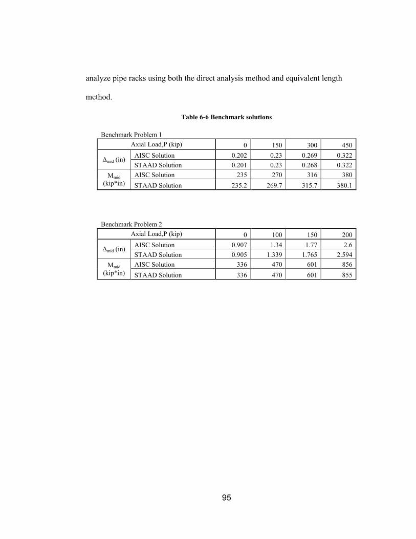
95
analyze pipe racks using both the direct analysis method and equivalent length
method.
Table 6-6 Benchmark solutions
Benchmark Problem 1 Axial Load,P (kip) 0 150 300 450
Δmid (in) AISC Solution 0.202 0.23 0.269 0.322 STAAD Solution 0.201 0.23 0.268 0.322
Mmid (kip*in)
AISC Solution 235 270 316 380 STAAD Solution 235.2 269.7 315.7 380.1
Benchmark Problem 2
Axial Load,P (kip) 0 100 150 200
Δmid (in) AISC Solution 0.907 1.34 1.77 2.6 STAAD Solution 0.905 1.339 1.765 2.594
Mmid (kip*in)
AISC Solution 336 470 601 856 STAAD Solution 336 470 601 855
96
7. Comparison of Results
Both pinned base and fixed base support condition models were developed for
analysis and comparison of the three methods of stability analysis. See Appendix 1
for STAAD.Pro V8i input file for pipe rack analysis using the effective length
method. Appendix 2 and 3 contain similar inputs for the direct analysis and first
order method respectively. The first model was analyzed with a pinned base column.
The member sizes were chosen without regard to serviceability and picked only to
satisfy the load demand. First order method, effective length method and direct
analysis method were all applied to the model and the results compiled. A first order
linear elastic analysis was completed to provide a benchmark for comparison and
calculation of the ratio of second order drift to first order drift.
Table 7-1 shows the ratio of second order to first order drift (Δ2/Δ1) based on
the comparison of the benchmark linear elastic analysis to the effective length method
analysis. It should be noted that these maximum deflections are based on LRFD load
combinations. See Appendix 1 and 2 for details of LRFD load combinations. The
maximum Δ2/Δ1 ratio is calculated as 1.15.
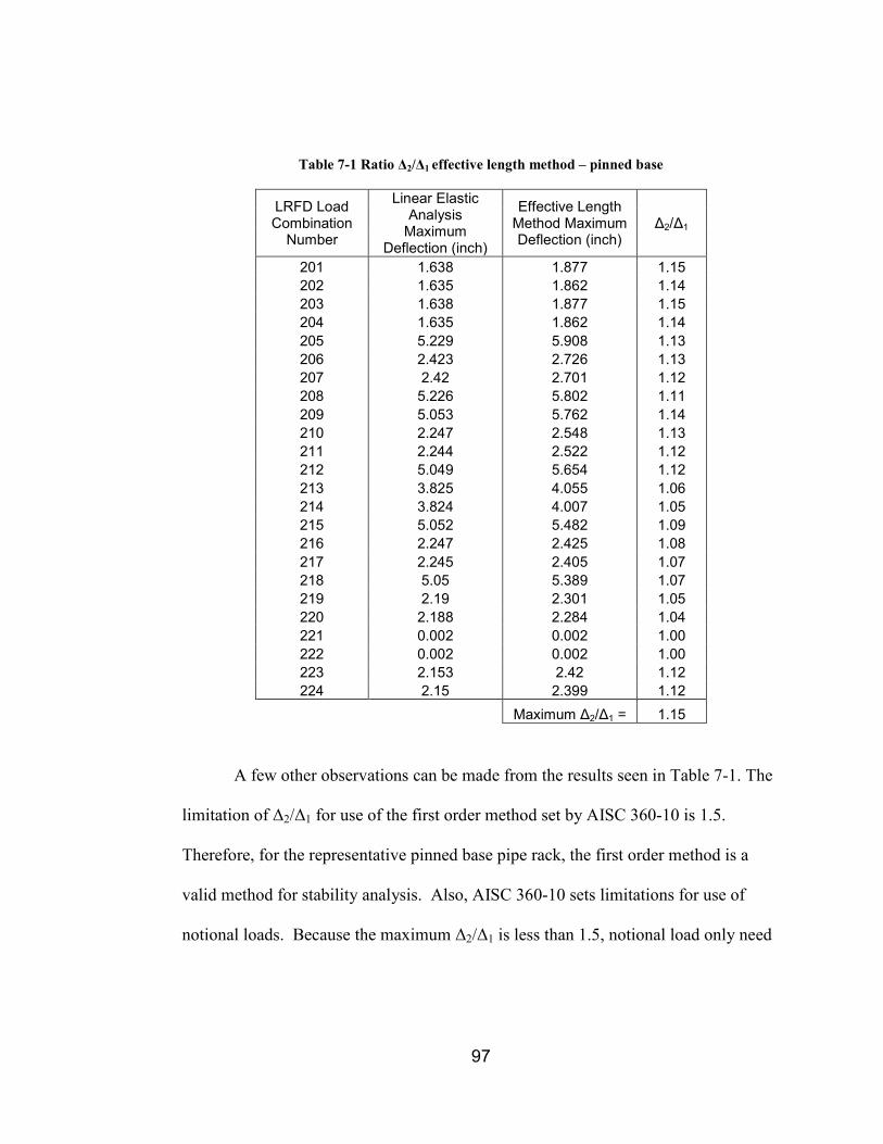
97
Table 7-1 Ratio Δ2/Δ1 effective length method – pinned base
LRFD Load Combination
Number
Linear Elastic Analysis
Maximum Deflection (inch)
Effective Length Method Maximum Deflection (inch)
Δ2/Δ1
201 1.638 1.877 1.15 202 1.635 1.862 1.14 203 1.638 1.877 1.15 204 1.635 1.862 1.14 205 5.229 5.908 1.13 206 2.423 2.726 1.13 207 2.42 2.701 1.12 208 5.226 5.802 1.11 209 5.053 5.762 1.14 210 2.247 2.548 1.13 211 2.244 2.522 1.12 212 5.049 5.654 1.12 213 3.825 4.055 1.06 214 3.824 4.007 1.05 215 5.052 5.482 1.09 216 2.247 2.425 1.08 217 2.245 2.405 1.07 218 5.05 5.389 1.07 219 2.19 2.301 1.05 220 2.188 2.284 1.04 221 0.002 0.002 1.00 222 0.002 0.002 1.00 223 2.153 2.42 1.12 224 2.15 2.399 1.12
Maximum Δ2/Δ1 = 1.15
A few other observations can be made from the results seen in Table 7-1. The
limitation of Δ2/Δ1 for use of the first order method set by AISC 360-10 is 1.5.
Therefore, for the representative pinned base pipe rack, the first order method is a
valid method for stability analysis. Also, AISC 360-10 sets limitations for use of
notional loads. Because the maximum Δ2/Δ1 is less than 1.5, notional load only need

98
be applied to the gravity only load combinations for use in the effective length
method.
Table 7-2 shows the ratio of second order to first order drift (Δ2/Δ1) based on
the comparison of the benchmark linear elastic analysis to the direct analysis method
analysis. As expected, the ratio Δ2/Δ1 is slightly higher based on the reduction in
stiffness. The benchmark first order linear elastic analysis for this comparison
included a reduced stiffness used in analysis. The increase in the ratio Δ2/Δ1 seen in
Table 7-2 shows that the reduction in stiffness can amplify the second order effects.
The maximum ratio Δ2/Δ1 is 1.21. Because the ratio Δ2/Δ1 is less than 1.7 (reduced
stiffness is used to calculate drift), notional load need only be applied in the gravity
only load combinations. (AISC 360-10)

99
Table 7-2 Ratio Δ2/Δ1 direct analysis method – pinned base
LRFD Load Combination
Number
Linear Elastic Analysis Maximum Deflection
(inch) - Reduced Stiffness
Effective Length Method Maximum Deflection (inch)
Δ2/Δ1
201 2.048 2.477 1.21 202 2.043 2.472 1.21 203 2.048 2.477 1.21 204 2.043 2.472 1.21 205 6.536 7.68 1.18 206 3.029 3.562 1.18 207 3.025 3.558 1.18 208 6.532 7.676 1.18 209 6.316 7.518 1.19 210 2.809 3.339 1.19 211 2.805 3.335 1.19 212 6.312 7.514 1.19 213 4.782 5.147 1.08 214 4.78 5.145 1.08 215 6.315 7.003 1.11 216 2.809 3.112 1.11 217 2.806 3.109 1.11 218 6.313 7 1.11 219 2.737 2.92 1.07 220 2.735 2.919 1.07 221 0.002 0.002 1.00 222 0.002 0.002 1.00 223 2.691 3.163 1.18 224 2.687 3.158 1.18
Maximum Δ2/Δ1 = 1.21
Both Table 7-1 and 7-2 show the importance of consideration of stability
analysis in design for pinned base conditions. For the representative pinned base
model, stability analysis can amplify the deformation by up to 21% for this specific
model. Deformation may not always be the focus of analysis and design but when

100
checking serviceability limits, stability analysis can increase deformations
significantly when compared to an elastic first order analysis.
The first order method was performed on the same model but as the method
name implies, only a first order analysis is done and therefore the ratio Δ2/Δ1 cannot
be directly calculated based on the drifts alone. However, based on the results of the
previous two analyses, the ratio Δ2/Δ1 will be well below the 1.5 limitation set be
AISC 360-10. Therefore the first order method is a valid type of stability analysis for
the representative pinned base pipe rack.
Demand to capacity for members should also be used when comparing the
types of stability analysis methods. Maximum demand to capacity ratio for both
column and beam design is shown in Table 7-3.
Table 7-3 Maximum demand to capacity ratio – pinned base
Column (10X49) Maximum Demand to Capacity Ratio Linear Elastic
Analysis First Order
Method Effective Length
Method Direct Analysis
Method 0.665 0.78 0.977 0.76
Beam (W10X33) Maximum Demand to Capacity Ratio Linear Elastic
Analysis First Order
Method Effective Length
Method Direct Analysis
Method 0.834 0.966 0.914 0.943
The linear elastic analysis was included as a benchmark for comparison. The
linear elastic analysis can be seen to underestimate the demand to capacity ratios of

101
members, sometimes significantly. When comparing the direct analysis method and
the first order method, it can be seen that the demand to capacity ratio is slightly
higher when using the first order method. This is to be expected since the first order
method is a simplification of the direct analysis built on conservative assumptions
which will envelope the design. The effective length method has slightly higher
ratios for column design and slightly lower for beam design. As discussed in
previous sections for the effective length method, the column strength equations are
adjusted using K to account for reduction in stiffness, but the moment can be
underestimated for beams and connections which resist column rotation. The actual
demand forces are listed in Table 7-4.
Table 7-4 Maximum demand forces – pinned base
Column (W12X53) Maximum Forces Linear Elastic
Analysis First Order
Method Effective
Length Method Direct Analysis
Method Strong Axis Moment (kip*ft) 102.94 130.34 122.41 126.83 Axial Load (kip) 54.88 58.61 56.9 57.63 Beam (W12X40) Maximum Forces Linear Elastic
Analysis First Order
Method Effective
Length Method Direct Analysis
Method Strong Axis Moment (kip*ft) 97.02 112.42 106.44 109.82 Axial Load (kip) 5.46 5.74 5.72 5.92
Based on Table 7-3 and 7-4 good correlation can be seen between the
methods. The demand to capacity ratios for each method show results that are

102
expected based on the theory used to develop each method. The member forces have
slight variation between methods based on the slight differences required in analysis
in the methods. All results show similar relationships between each method. It should
be noted that varying geometry could have a significant effect on the ratio Δ2/Δ1
which could limit the use of either the first order method or effective length method.
In general for the pinned base support condition, columns have relatively low axial
demand when compared to the compression failure load Py. Large moments are
developed in both the columns and beams and therefore the majority of the member
capacity is used to resist the moment demand
Similar tables to those seen above were also developed based on the fixed
base support condition which can be seen on the following pages.

103
Table 7-5 Ratio Δ2/Δ1 effective length method – fixed base
LRFD Load Combination
Number
Linear Elastic Analysis
Maximum Deflection (inch)
Effective Length Method Maximum Deflection (inch)
Δ2/Δ1
201 0.687 0.72 1.05 202 0.682 0.715 1.05 203 0.687 0.72 1.05 204 0.682 0.715 1.05 205 2.03 2.116 1.04 206 0.856 0.892 1.04 207 0.852 0.886 1.04 208 2.026 2.105 1.04 209 2.148 2.246 1.05 210 0.974 1.017 1.04 211 0.97 1.01 1.04 212 2.144 2.233 1.04 213 1.442 1.47 1.02 214 1.44 1.465 1.02 215 2.147 2.208 1.03 216 0.973 0.999 1.03 217 0.971 0.995 1.02 218 2.145 2.197 1.02 219 0.936 0.952 1.02 220 0.935 0.949 1.01 221 0.002 0.002 1.00 222 0.002 0.002 1.00 223 0.812 0.846 1.04 224 0.808 0.841 1.04
Maximum Δ2/Δ1 = 1.05
When comparing the fixed base ratio Δ2/Δ1 for the effective length method, it
can be seen that the maximum value is 1.05. While this is slightly less than for the
pinned base support condition model, it still shows the significance of stability
analysis in design. Table 7-6 below shows the same ratio Δ2/Δ1 for the direct analysis
with both the linear elastic and direct analysis using the reduced stiffness in
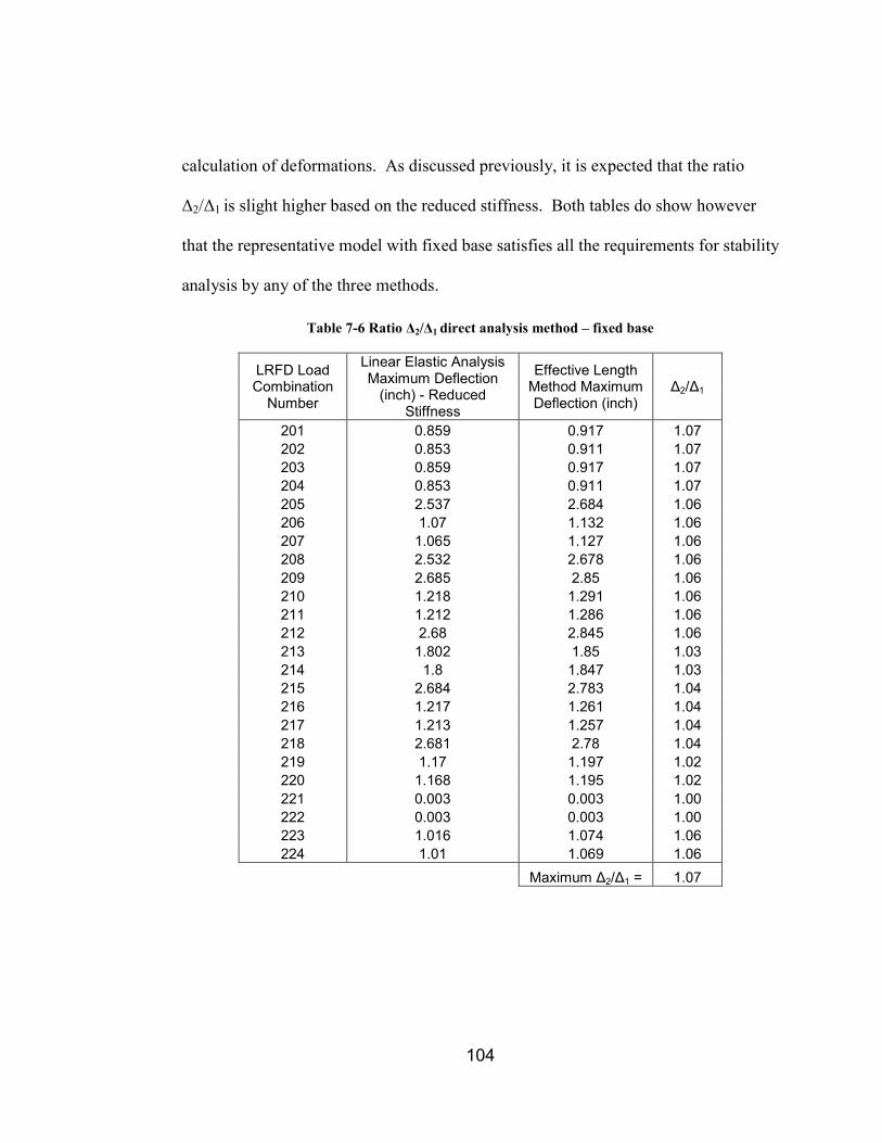
104
calculation of deformations. As discussed previously, it is expected that the ratio
Δ2/Δ1 is slight higher based on the reduced stiffness. Both tables do show however
that the representative model with fixed base satisfies all the requirements for stability
analysis by any of the three methods.
Table 7-6 Ratio Δ2/Δ1 direct analysis method – fixed base
LRFD Load Combination
Number
Linear Elastic Analysis Maximum Deflection
(inch) - Reduced Stiffness
Effective Length Method Maximum Deflection (inch)
Δ2/Δ1
201 0.859 0.917 1.07 202 0.853 0.911 1.07 203 0.859 0.917 1.07 204 0.853 0.911 1.07 205 2.537 2.684 1.06 206 1.07 1.132 1.06 207 1.065 1.127 1.06 208 2.532 2.678 1.06 209 2.685 2.85 1.06 210 1.218 1.291 1.06 211 1.212 1.286 1.06 212 2.68 2.845 1.06 213 1.802 1.85 1.03 214 1.8 1.847 1.03 215 2.684 2.783 1.04 216 1.217 1.261 1.04 217 1.213 1.257 1.04 218 2.681 2.78 1.04 219 1.17 1.197 1.02 220 1.168 1.195 1.02 221 0.003 0.003 1.00 222 0.003 0.003 1.00 223 1.016 1.074 1.06 224 1.01 1.069 1.06
Maximum Δ2/Δ1 = 1.07

105
Table 7-7 Maximum demand to capacity ratio – fixed base
Column (W10X33) Maximum Demand to Capacity Ratio Linear Elastic
Analysis First Order
Method Effective Length
Method Direct Analysis
Method 0.864 0.908 0.887 0.896
Beam (W10X26) Maximum Demand to Capacity Ratio Linear Elastic
Analysis First Order
Method Effective Length
Method Direct Analysis
Method 0.835 0.876 0.859 0.868
Table 7-8 Maximum demand forces – fixed base
Column (W10X33) Maximum Forces Linear Elastic
Analysis First Order
Method Effective
Length Method Direct Analysis
Method Strong Axis Moment (kip*ft) 60.136 63.35 62.35 63.19 Axial Load (kip) 46.03 46.83 46.42 46.56 Beam (W10X26) Maximum Forces Linear Elastic
Analysis First Order
Method Effective
Length Method Direct Analysis
Method Strong Axis Moment (kip*ft) 61.1 64.12 62.91 63.56 Axial Load (kip) 5.12 5.23 5.15 5.15
In general, the first order method tends to be inherently more conservative
based on the analysis assumptions which increase demand to account for the second
order effects and reduction in stiffness. The effective length method on the other
hand, tends to underestimate the demand while the capacity is adjusted to account for

106
the underestimation in demand by using the K factor. The direct analysis method will
typically provide the most accurate results.
When comparing the two support condition models, several observations can
be made. The representative fixed base model tends to have slightly lower second
order effects compared to the pinned based model. The fixed base model also tends
to have lower deformations even when smaller member sizes are used. When
demand to capacity is the only consideration in design, the deformations can easily
become relatively significant and exceed standard serviceability limits especially in
the case of pinned base support conditions.
Serviceability limits were considered for additional analysis models. The
representative pin based model was the focus based on large drift ratios when strength
was the only consideration. A target serviceability limit was set at H/200. Members
were resized based on this target and the results can be seen in the following tables.
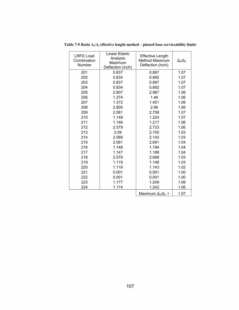
107
Table 7-9 Ratio Δ2/Δ1 effective length method – pinned base serviceability limits
LRFD Load Combination
Number
Linear Elastic Analysis
Maximum Deflection (inch)
Effective Length Method Maximum Deflection (inch)
Δ2/Δ1
201 0.837 0.897 1.07 202 0.834 0.892 1.07 203 0.837 0.897 1.07 204 0.834 0.892 1.07 205 2.807 2.987 1.06 206 1.374 1.46 1.06 207 1.372 1.451 1.06 208 2.805 2.96 1.06 209 2.581 2.758 1.07 210 1.149 1.224 1.07 211 1.146 1.217 1.06 212 2.579 2.733 1.06 213 2.09 2.155 1.03 214 2.089 2.142 1.03 215 2.581 2.691 1.04 216 1.148 1.194 1.04 217 1.147 1.188 1.04 218 2.579 2.668 1.03 219 1.119 1.148 1.03 220 1.118 1.143 1.02 221 0.001 0.001 1.00 222 0.001 0.001 1.00 223 1.177 1.249 1.06 224 1.174 1.242 1.06
Maximum Δ2/Δ1 = 1.07

108
Table 7-10 Ratio Δ2/Δ1 direct analysis method – pinned base serviceability limits
LRFD Load Combination
Number
Linear Elastic Analysis Maximum Deflection
(inch) - Reduced Stiffness
Effective Length Method Maximum Deflection (inch)
Δ2/Δ1
201 1.046 1.151 1.10 202 1.043 1.147 1.10 203 1.046 1.151 1.10 204 1.043 1.147 1.10 205 3.509 3.807 1.08 206 1.718 1.865 1.09 207 1.715 1.862 1.09 208 3.506 3.804 1.08 209 3.227 3.522 1.09 210 1.436 1.566 1.09 211 1.433 1.563 1.09 212 3.223 3.519 1.09 213 2.613 2.716 1.04 214 2.611 2.715 1.04 215 3.226 3.401 1.05 216 1.435 1.512 1.05 217 1.433 1.51 1.05 218 3.224 3.399 1.05 219 1.398 1.447 1.04 220 1.397 1.446 1.04 221 0.002 0.002 1.00 222 0.002 0.002 1.00 223 1.471 1.596 1.08 224 1.468 1.593 1.09
Maximum Δ2/Δ1 = 1.10
Comparing the results of the pinned base (Tables 7-1 and 7-2) with the pinned
base with serviceability limits imposed (Tables 7-9 and 7-10) shows an overall
reduction in second order effects when serviceability controls the design. The overall
structural stiffness is increased to limit deflections due to serviceability and therefore
second order effects are minimized since the loads are acting on a less deformed
shape.

109
Demand to capacity ratios show similar results when compared to previous
results. Table 7-11 shows demand to capacity ratios when serviceability limits are
imposed on the design. The demand to capacity ratios are much lower based on the
additional stiffness required to meet serviceability limits.
Table 7-11 Maximum demand to capacity ratio – pinned base serviceability limits
Column (W12X65) Maximum Demand to Capacity Ratio Linear Elastic
Analysis First Order
Method Effective Length
Method Direct Analysis
Method 0.418 0.452 0.483 0.447
Beam (W12X45) Maximum Demand to Capacity Ratio Linear Elastic
Analysis First Order
Method Effective Length
Method Direct Analysis
Method 0.515 0.555 0.539 0.547
As seen in the results, both from the representative models and the cantilever
column example, the effective length method tends to underestimate the moment
demand in both the column and any beam or connection that resists column rotation.
This fact should be considered in design if the effective length method is used for
stability analysis.
The results also show the importance of stability analysis. Linear elastic
analysis is not sufficient especially when designing moment frames. The results from
above showed that the demand to capacity ratio could be underestimated by
approximately 10-20% for the worst case when conducting a linear elastic analysis.

110
Varying the stiffness or geometry could easily produce greater errors in analysis if
stability analysis is not considered.

111
8. Conclusions
For the representative pipe rack model, both pinned and fixed base conditions,
the first order, effective length, and direct analysis methods were all found to be valid
methods of stability analysis according to AISC 360-10. When the ratios Δ2/Δ1 and
Pr/Py are below the limits specified by AISC 360-10, all methods gave comparable
results. Several observations on each method can be made based on the analysis and
results.
The direct analysis method provides the most accurate results since reduction
in stiffness is considered in analysis. There are also many benefits in application of
this method with the most significant benefit being that the effective length factor K
can be set to 1 for all cases. This can significantly simplify calculations required to
perform analysis especially for moment frames. Additionally, the direct analysis
method has no limitations for use. Without limitations, no validation after analysis is
required and therefore less time is required for this method. However, the best results
from use of this method typically come from utilization of modern analysis software
capable of performing rigorous second order analysis. Although an approximate
second order analysis can be done by hand, this can become quite tedious and time
consuming when other methods could produce similar results with less work.

112
The first order analysis is a mathematically simplified analysis method. The
greatest benefit as the name implies, is that the method only requires a first order
analysis. As with the direct analysis method, K can also be set at 1 for all cases.
Based on the above simplifications, analysis can be significantly simplified. The
simplified analysis tends to be the most beneficial for hand calculations of frames.
The simplifications made in development of the method do however impose
limitations on use. While the analysis portion may be less intensive, the post-analysis
validation required can sometimes outweigh the benefits if the simplified analysis.
Additionally, several iterations in analysis may be required to achieve the most
accurate results since notional loads are calculated based on target drift limits.
Application of notional load in all load combinations can also create significantly
more load combinations which need to be considered in design. Simplifications in
analysis also tend to create the most conservative results when compared to other
methods of stability analysis.
The effective length method is probably the most well known method for
stability analysis. However as the name implies, the effective length factor K must be
calculated. Based on the discussions in previous sections, this can become very
complex even for relatively simple structures. The accuracy of the effective length
method is critically linked to accurate calculation of the effective length factor.
Various methods for determining K have been developed but the most widely known
is still the alignment charts. When using the alignment charts from AISC 360-10 the
113
engineer should be aware of the assumptions made in the development of the charts
and the limitations for use. AISC 360-10 has set limitations for use of this method.
Verification of applicability of effective length method after analysis could limit the
use of this method. Second order effects should be considered in design which can be
done using either a rigorous or approximate analysis. Results from this method show
that the moment demand for beams and connections that resist column rotation can be
underestimated. The underestimation of moments in elements resisting column
rotation is due to no reduction in stiffness considered in analysis. The engineer
should be aware of the underestimation of moment demand when designing beams
and connections with results found using the effective length method.
When comparing the pro’s and con’s of each method, some observations can
be made. If modern software analysis is available, the direct analysis method will
most likely require the least amount of work to achieve the most accurate results.
Although the effective length method is the most well known, engineers should be
aware of limitations and the tendency for underestimation of moments in results. The
first order method can be a powerful method if certain limitations are met and slightly
conservative results are acceptable. However, with modern analysis software, the
first order method will likely see limited applicability unless calculations are
completed by hand.
Stability analysis as it relates specifically to pipe rack structures provides
several points of interest. Base support conditions have a relatively large influence on

114
results of stability analysis. Pinned base pipe racks could have large deformations
which tend to produce larger second order effects. If fixed base support conditions
can be developed, member strength can be further utilized before serviceability limits
are reached. However, fixed base support conditions in many cases can be difficult to
achieve.
If each method is applied appropriately to pipe rack structures, based on the
results above, good correlation can be seen between the first order, effective length
and direct analysis methods. However, AISC 360-10 limitation must be verified for
use of the first order and effective length methods on a case by case basis. For the
representative models used above, all three methods met AISC 360-10 requirements
and were found acceptable for stability analysis.
Pipe racks moment frames tend to support relatively large lateral loads
through flexural resistance. Because the majority of the member capacity is used to
resist the lateral loads, little capacity is left to resist axial loads, therefore the member
is sized based primarily on the flexural demand. Based on the lower axial demands,
the additional reduction in stiffness used in the direct analysis method due to large
axial demand typically is not required.
The representative pipe rack chosen for analysis was a moderately simple
frame and calculation of the effective length factor was relatively straightforward.
However, actual pipe racks may require more complex structures which can greatly
complicate the calculation of the effective length factor. Based on the possibility for

115
complex effective length factor calculations, the direct analysis and first order method
could be much less calculation intensive and provide more accurate results.
Based on the above results and observations, I recommend the direct analysis
as the first choice in stability analysis for pipe racks. While both the effective length
and first order method provide relatively accurate results as long their respective
requirements are met the direct analysis provides the most accurate results and has no
limitations for use. The direct analysis method can also be the simplest method to
apply if modern software analysis is utilized as no front end calculations or post-
analysis verification are required.

116
REFERENCES
American Institute of Steel Construction (AISC). (2005). “Specification for structural
steel buildings (ANSI/AISC 360-05).” American Institute of Steel
Construction, Inc. Chicago.
American Institute of Steel Construction (AISC). (2010) “Specification for structural
steel buildings (ANSI/AISC 360-10).” American Institute of Steel
Construction, Inc. Chicago.
American Institute of Steel Construction (AISC). (2010) “Code of standard practice
for steel buildings and bridges (AISC 303-10).” American Institute of Steel
Construction, Inc. Chicago.
ASCE Task Committee on Effective Length. (1997) “Effective length and notional
load approaches for assessing frame stability: implications for American steel
design.” American Society of Civil Engineers, New York.
American Society of Civil Engineers (ASCE). (2006) “Minimum Design Loads for
Buildings and Other Structures (ASCE 7-05).” American Society of Civil
Engineers, Reston, VA.
American Society of Civil Engineers (ASCE). (2010) “Minimum design loads for
buildings and other structures (ASCE 7-10).” American Society of Civil
Engineers, Reston, VA.

117
American Society of Civil Engineers (ASCE). (2011) “Wind load for petrochemical
and other industrial facilities.” American Society of Civil Engineers, Reston,
VA.
American Society of Civil Engineers (ASCE). (1997) “Guideline for seismic
evaluation and design of petrochemical facilities.” American Society of Civil
Engineers, Reston, VA.
Bathe, K. J. (1995). “Finite element procedures.” Prentice, Upper Saddle River, NJ.
Hall.
Bendapudi, K. V. (2010). “Structural design of steel pipe support structures.”
Structure Magazine, 17 (2), 6-8.
Bendapudi, K. V. (2010). “Discussion on structural design of steel pipe support
structures.” Structure Magazine, 17 (11), 38-40.
Canada Department of Railways and Canals. (1919). “The Quebec bridge over the
St. Lawrence River near the city of Quebec on the line of the Canadian
National Railways (Report No. 1).” Canada Department of Railways and
Canals, Ottawa Canada
Chen, W. F., and Lui, E. M. (1991). “Stability design of steel frames.” CRC Press,
Boca Raton, FL.
Crisfield, M. A. (1991). “Nonlinear finite element analysis of solids and structures.”
Wiley, New York.

118
Deierlein, G. G., Hajjar, J. F., Yura, J. A., White, D. W., and Baker, W. F. (2002).
“Proposed new provisions for frame stability using second-order analysis.”
Proceedings 2002 Annual Technical Session, Seattle, April. Structural
Stability Research Council, Rolla, MO.
Delatte, N. J. (2009). “Beyond failure: forensic case studies for civil engineers.”
ASCE Press, Reston, VA, 51-70.
Drake, R.M., & Walter, R.J. (2010). ”Design of structural steel pipe racks.” AISC
Engineering Journal, 47 (4). 241-252.
Euler, L. (1744). “Methodus inveniendi lineas curvas….” Bousquet, Lausanne.
Ericksen, J. R. (2011). “A how-to approach to notional loads.” AISC Modern Steel
Construction, 51 (1). 44-45
Folse, M. D., and Nowak, P. S. (1995). “Steel rigid frames with leaning columns –
1993 LRFD example.” AISC Engineering Journal, 32 (4). 125-131.
Galambos, T. V. ed (1998). “Guide to stability design criteria for metal structures, 5th
Edition.” John Wiley & Sons, Inc., Hoboken, NJ.
Geschwindner, L. F. (2002). “A practical look at frame analysis stability and leaning
columns.” AISC Engineering Journal, 39 (4). 167-181
Geschwindner, L. F. (2009). “Design for stability using 2005 AISC specification.”
seminar notes, presented Sept 18, 2009, Sponsored by AISC, Chicago, IL.
Huber, A. W., and Beedle, L. S. (1954). “Residual stress and compressive strength of
steel.” Welding Journal, December. 589-614.
119
Hibbeler, R. C. (2005). “Mechanics of materials 6th Edition.” Pearson Prentice Hall,
New Jersey.
Kanchanalai, T. (1977). “The Design and Behavior of Beam-Columns in Unbraced
Steel Frames.” AISI Project Number 189, Report Number 2, Civil
Engineering/Structures Research Laboratories, University of Texas, Austin,
TX.
Kanchanalai, T., and Lu, L.-W. (1979) “Analysis and design of framed columns
under minor axis bending.” AISC Engineering Journal, 16 (2). 29-41.
Kuchenbecker, G. H., White, D. W., and Surovek-Malek, A. E. (2004). “Simplified
design of building frames using first-order analysis and K = 1.” Proceedings
of the Annual Technical Session and Meetings, Long Beach, CA, March 24-
27, 2004. Structural Stability Research Council, Rolla, MO. 119-138.
LeMessurier, W. J. (1976). “A practical method of second order analysis part 1 – pin
jointed systems.” AISC Engineering Journal, 13 (4). 89-96
LeMessurier, W. J. (1977). “A practical method of second order analysis part 2 –
rigid frames.” AISC Engineering Journal, 14 (2). 49-67
LeMessurier, W. J. (1995). “Simplified K factors for stiffness controlled designs“,
restructuring: America and beyond.” Proceedings of ASCE Structures
Congress XIII, Boston, MA , April 2-5. American Society of Civil Engineers,
New York. 1797-1812.
120
Maleck, A.E., and White, D.W. (1998). “Effects of imperfections on steel framing
systems.” Proceedings 1998 Annual Technical Sessions, Atlanta, September.
Structural Stability Research Council, Rolla, MO.
Maleck, A. E., and White, D. W. (2003). “Direct analysis approach for the assessment
of frame stability: verification studies.” Proceedings Annual Technical
Sessions, Structural Stability Research Council, Rolla, MO. 18
McGuire, W., Gallegher, R. H., and Ziemian, R. D. (2000). “Matrix structural
analysis, 2nd Edition.” John Wiley & Sons Inc., Hoboken, NJ.
Nair, S. R. (2009). “A model specification for stability design by direct analysis.”
AISC Engineering Journal, 46 (1). 29-38
Process Industry Practices (PIP) (2007). “Structural design criteria (PIP STC01015).”
Construction Industry Institute, Process Industry Practices, Austin, TX.
Powell, G. H. (2010). “Modeling for structural analysis: behavior and basics.”
Computers and Structures, Inc. Berkeley, CA.
Rutenberg, A. (1981). “A direct p-delta analysis using stand plane frame computer
programs.” ASCE Journal Engineering Mechanical Division, 86 (EM1). 61-
78.
Rutenberg, A. (1982). “Simplified p-delta analysis for asymmetric structures.” ASCE
Journal Engineering Mechanical Division, 108 (ST9). 1995-2013.

121
Salmon, C. G., and Johnson, J. E. (2008). “Steel structures: design and behavior,
emphasizing load and resistance design 5th Edition.” Harper Collins, New
York.
STAAD.Pro V8i (2007). “Technical Reference Manual.” Bentley Systems, Inc.,
Yorba Linda, CA.
Surovek-Maleck, A. E., and White, D. W. (2004a). “Alternative approaches for
elastic analysis and design of steel frames. I: overview.” ASCE Journal of
Structural Engineering, 130 (8). 1186-1196.
Surovek-Maleck, A.E., and White, D.W. (2004b) “Alternative approaches for elastic
analysis and design of steel frames. II: verification studies.” ASCE Journal of
Structural Engineering, 130 (8). 1197-1205.
Trakov, J. (1986). “Quebec bridge: a disaster in the making.” Invention &
Technology, American Heritage, 1 (4). 10-17
Vinnakota, S. (2006). “Steel structures: behavior and LRFD”, 1st Edition.” McGraw-
Hill, New York.
White, D. W., and Hajjar, J. F. (1991). “Application of second-order elastic analysis
in LRFD: research to practice.” AISC Engineering Journal, 28 (4). 133-148.
White, D. W., Surovek, A. E., Alemdar, B. N., Chang, C., Kim, Y. D., and
Kuchenbecker, G. H. (2006). “Stability analysis and design of steel building
frames using the AISC 2005 specification.” International Journal of Steel
Structures, 6. 71-91

122
White, D. W., Surovek, A. E., and Kin, S-C. (2007a). “Direct analysis and design
using amplified first-order analysis. part 1 – combined braced and gravity
framing systems.” AISC Engineering Journal, 44 (4). 305-322.
White, D. W., Surovek, A. E., and Chang, C-J. (2007b). “Direct analysis and design
using amplified first-order analysis. part 2 – moment frames and general
framing systems.” AISC Engineering Journal, 44 (4). 323-340.
Yang, C. H., Beedle, L. S., and Johnson, B. G. (1952). “Residual stress and the yield
strength of steel beams.” Welding Journal, April 1952. 589-614.
Yang, C. H., and Quo, S. R. (1994). “Theory and analysis of nonlinear framed
structures.” Prentice Hall, Upper Saddle River, NJ.
Yura, J. A. (1971). “The effective length of columns in unbraced frames.” .” AISC
Engineering Journal, 8 (2). 37-42.
Yura, J. A., Kanchanalai, T., and Chotichanathawenwong, S. (1996). “Verification of
steel beam-column design based on the AISC-LRFD method.” Proceeding 5th
International Colloquium Stability Metal Structures, Lehigh University,
Bethlehem, PA, Structural Stability Research Council, Rolla, MO. 21-30.
Ziemianm, R. A. ed (2010). “Guide to stability design criteria for metal structures, 6th
Edition.” John Wiley & Sons, Inc., Hoboken, NJ.

123
Appendix A – STAAD Input Pinned Base Analysis - Effective Length Method STAAD SPACE START JOB INFORMATION ENGINEER DATE 1-25-2012 ENGINEER NAME DAN END JOB INFORMATION * *EQUIVALENT LENGTH METHOD *PINNED BASE MODEL * INPUT WIDTH 79 * *DEFINES JOINT LOCATIONS UNIT FEET KIP JOINT COORDINATES 1 0 0 0; 2 0 20 0; 3 0 25 0; 4 0 30 0; 5 0 35 0; 6 15 0 0; 7 15 20 0; 8 15 25 0; 9 15 30 0; 10 15 35 0; * *DEFINES MEMBERS MEMBER INCIDENCES 1 1 2; 2 2 3; 3 3 4; 4 4 5; 5 2 7; 6 3 8; 7 4 9; 8 5 10; 9 6 7; 10 7 8; 11 8 9; 12 9 10; * *DEFINE PROPERITIES OF STEEL DEFINE MATERIAL START ISOTROPIC STEEL E 4.176e+006 POISSON 0.3 DENSITY 0.489024 ALPHA 6.5e-006 DAMP 0.03 END DEFINE MATERIAL * * *DEFINE MEMBER SHAPE MEMBER PROPERTY AMERICAN 1 TO 4 9 TO 12 TABLE ST W10X49 5 TO 8 TABLE ST W10X33 * * CONSTANTS *SETS ALL MEMBERS TO BE STEEL MATERIAL STEEL ALL *

124
*DEFINES SUPPORT CONDITIONS SUPPORTS 1 6 PINNED 2 TO 5 7 TO 10 FIXED BUT FX FY MX MY MZ * *DEFINES WIND VELOCITY PRESSURE QZ FOR APPLICATION DEFINE WIND LOAD TYPE 1 INT 0.02127 0.02127 0.02252 0.02352 0.02452 0.02602 HEIG 0 15 20 25 30 40 * * * ********************************** *PRIMARY LOAD CASES ********************************** * LOAD 1 DEAD LOAD (DS) STEEL AND FIREPROOFING *SELFWEIGHT OF THE STRUCTURE PLUS 10% FOR CONNECTIONS SELFWEIGHT Y -1.1 * * * * LOAD 2 OPERATING DEAD LOAD (DO) *40 PSF UNIFORM LOAD OVER TRIBUTARY AREA *40PSF*20FEET = 800 PLF = 0.8 KLF MEMBER LOAD 5 TO 8 UNI GY -0.8 * * * LOAD 3 EMPTY DEAD LOAD (DE) *60% OF OPERATING DEAD LOAD MEMBER LOAD 5 TO 8 UNI GY -0.48 * * * LOAD 4 TEST DEAD LOAD (DT) *40 PSF UNIFORM LOAD OVER TRIBUTARY AREA *40PSF*20FEET = 800 PLF = 0.8 KLF MEMBER LOAD 5 TO 8 UNI GY -0.8 * * * LOAD 5 WIND LOAD X DIRECTION (WX) *APPLIES PRESSURE GRADIENT TO MEMBERS IN MODEL, *FACTOR = (GUST * SHAPE FACTOR) *G = 0.85, CD = 2.0

125
*WIND LOAD ON STRUCTURAL MEMBERS *APPLIED BASED ON PROJECTED AREA WIND LOAD X 1.7 TYPE 1 OPEN *WIND ON PIPE OR CABLE TRAY JOINT LOAD 2 7 FX 0.371 3 8 FX 0.387 4 9 FX 0.404 5 10 FX 0.429 * * * LOAD 7 SEISMIC LOAD X DIRECTION (EX) *SEISMIC LOAD APPLIED BASED ON VERTICAL DISTRIBUTION JOINT LOAD 2 7 FX 0.475 3 8 FX 0.725 4 9 FX 1.05 5 10 FX 1.425 * * * LOAD 14 SEISMIC LOAD Y DIRECTION (EY) *PRIMARY LOADS 1 AND 2 MULTIPLIED BY 10% *LOAD 1 DEAD LOAD (DS) STEEL AND FIREPROOFING SELFWEIGHT Y -0.11 * *LOAD 2 OPERATING DEAD LOAD (DO) MEMBER LOAD 5 TO 8 UNI GY -0.08 * * * LOAD 9 PIPE FRICTION LOAD (FF) *10% OF OPERATING DEAD LOAD APPLIED LONGITUDINAL MEMBER LOAD 5 TO 8 UNI GZ 0.08 * * * LOAD 10 PIPE ANCHOR LOAD (AF) *5% OF OPERATING DEAD LOAD APPLIED TRANSVERSE MEMBER LOAD 5 TO 8 UNI GX 0.04 * * * LOAD 11 THERMAL EXPANSION FORCE (T) *DELTA T OF 0 DEGREES APPLIED TO ALL STRUCTURAL MEMBERS TEMPERATURE LOAD
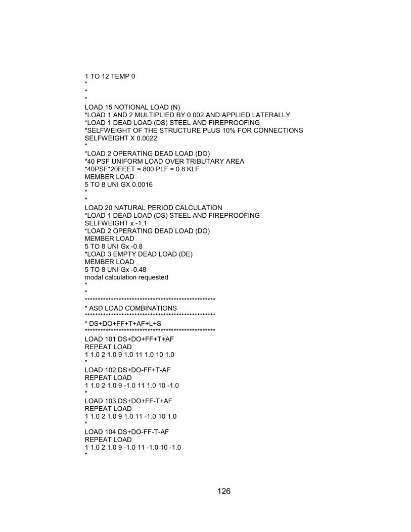
126
1 TO 12 TEMP 0 * * * LOAD 15 NOTIONAL LOAD (N) *LOAD 1 AND 2 MULTIPLIED BY 0.002 AND APPLIED LATERALLY *LOAD 1 DEAD LOAD (DS) STEEL AND FIREPROOFING *SELFWEIGHT OF THE STRUCTURE PLUS 10% FOR CONNECTIONS SELFWEIGHT X 0.0022 * *LOAD 2 OPERATING DEAD LOAD (DO) *40 PSF UNIFORM LOAD OVER TRIBUTARY AREA *40PSF*20FEET = 800 PLF = 0.8 KLF MEMBER LOAD 5 TO 8 UNI GX 0.0016 * * LOAD 20 NATURAL PERIOD CALCULATION *LOAD 1 DEAD LOAD (DS) STEEL AND FIREPROOFING SELFWEIGHT x -1.1 *LOAD 2 OPERATING DEAD LOAD (DO) MEMBER LOAD 5 TO 8 UNI Gx -0.8 *LOAD 3 EMPTY DEAD LOAD (DE) MEMBER LOAD 5 TO 8 UNI Gx -0.48 modal calculation requested * * ************************************************** * ASD LOAD COMBINATIONS ************************************************** * DS+DO+FF+T+AF+L+S ************************************************** LOAD 101 DS+DO+FF+T+AF REPEAT LOAD 1 1.0 2 1.0 9 1.0 11 1.0 10 1.0 * LOAD 102 DS+DO-FF+T-AF REPEAT LOAD 1 1.0 2 1.0 9 -1.0 11 1.0 10 -1.0 * LOAD 103 DS+DO+FF-T+AF REPEAT LOAD 1 1.0 2 1.0 9 1.0 11 -1.0 10 1.0 * LOAD 104 DS+DO-FF-T-AF REPEAT LOAD 1 1.0 2 1.0 9 -1.0 11 -1.0 10 -1.0 *

127
************************************************** * DS+DO+AF+W ************************************************** LOAD 105 DS+DO+AF+WX REPEAT LOAD 1 1.0 2 1.0 10 1.0 5 1.0 * LOAD 106 DS+DO-AF+WX REPEAT LOAD 1 1.0 2 1.0 10 -1.0 5 1.0 * LOAD 107 DS+DO+AF-WX REPEAT LOAD 1 1.0 2 1.0 10 1.0 5 -1.0 * LOAD 108 DS+DO-AF-WX REPEAT LOAD 1 1.0 2 1.0 10 -1.0 5 -1.0 * ************************************************** * DS+DO+AF+0.7E ************************************************** LOAD 109 DS+DO+AF+0.7EX+0.7EY REPEAT LOAD 1 1.0 2 1.0 10 1.0 7 0.7 14 0.7 * LOAD 110 DS+DO-AF+0.7EX+0.7EY REPEAT LOAD 1 1.0 2 1.0 10 -1.0 7 0.7 14 0.7 * LOAD 111 DS+DO+AF-0.7EX+0.7EY REPEAT LOAD 1 1.0 2 1.0 10 1.0 7 -0.7 14 0.7 * LOAD 112 DS+DO-AF-0.7EX+0.7EY REPEAT LOAD 1 1.0 2 1.0 10 -1.0 7 -0.7 14 0.7 * ************************************************** * DS+DE+W ************************************************** LOAD 113 DS+DE+WX REPEAT LOAD 1 1.0 3 1.0 5 1.0 * LOAD 114 DS+DE-WX REPEAT LOAD 1 1.0 3 1.0 5 -1.0 * **************************************************

128
* 0.9DS+0.6DO+AF+0.7E ************************************************** LOAD 115 0.9DS+0.6DO+AF+0.7EX-0.7EY REPEAT LOAD 1 0.9 2 0.6 10 1.0 7 0.7 14 -0.7 * LOAD 116 0.9DS+0.6DO-AF+0.7EX-0.7EY REPEAT LOAD 1 0.9 2 0.6 10 -1.0 7 0.7 14 -0.7 * LOAD 117 0.9DS+0.6DO+AF-0.7EX-0.7EY REPEAT LOAD 1 0.9 2 0.6 10 1.0 7 -0.7 14 -0.7 * LOAD 118 0.9DS+0.6DO-AF-0.7EX-0.7EY REPEAT LOAD 1 0.9 2 0.6 10 -1.0 7 -0.7 14 -0.7 * ************************************************** * 0.9(DS+DE)+0.7EE ************************************************** LOAD 119 0.9(DS+DE)+0.42EX-0.42EY REPEAT LOAD 1 0.9 3 0.9 7 0.42 14 -0.42 * LOAD 120 0.9(DS+DE)-0.42EX-0.42EY REPEAT LOAD 1 0.9 3 0.9 7 -0.42 14 -0.42 * ************************************************** * DS+DT+WP ************************************************** LOAD 121 DS+DT+WPX REPEAT LOAD 1 1.0 4 1.0 5 0.56 * LOAD 122 DS+DT-WPX REPEAT LOAD 1 1.0 4 1.0 5 -0.56 * * * * * ************************************************** * LRFD LOAD COMBINATIONS ************************************************** * 1.4(DS+DO+FF+T+AF) ************************************************** LOAD 201 1.4(DS+DO+FF+T+AF)
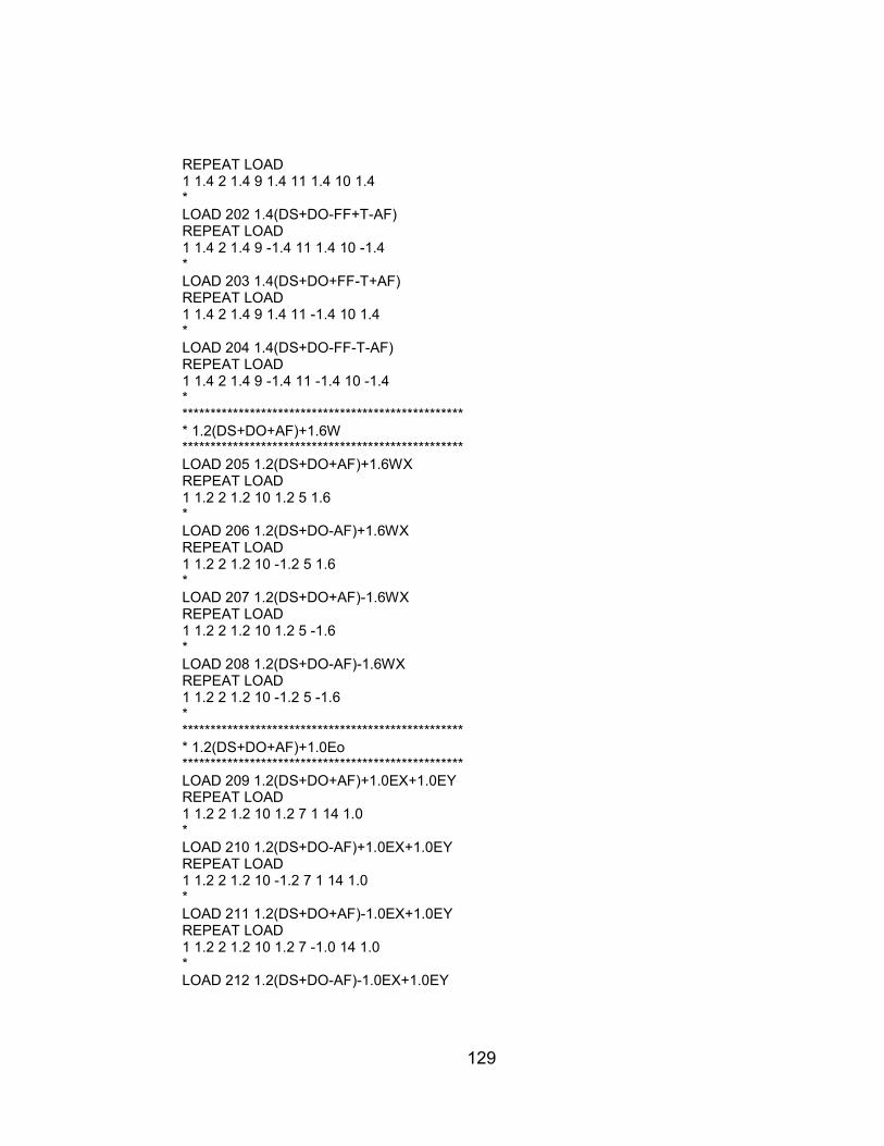
129
REPEAT LOAD 1 1.4 2 1.4 9 1.4 11 1.4 10 1.4 * LOAD 202 1.4(DS+DO-FF+T-AF) REPEAT LOAD 1 1.4 2 1.4 9 -1.4 11 1.4 10 -1.4 * LOAD 203 1.4(DS+DO+FF-T+AF) REPEAT LOAD 1 1.4 2 1.4 9 1.4 11 -1.4 10 1.4 * LOAD 204 1.4(DS+DO-FF-T-AF) REPEAT LOAD 1 1.4 2 1.4 9 -1.4 11 -1.4 10 -1.4 * ************************************************** * 1.2(DS+DO+AF)+1.6W ************************************************** LOAD 205 1.2(DS+DO+AF)+1.6WX REPEAT LOAD 1 1.2 2 1.2 10 1.2 5 1.6 * LOAD 206 1.2(DS+DO-AF)+1.6WX REPEAT LOAD 1 1.2 2 1.2 10 -1.2 5 1.6 * LOAD 207 1.2(DS+DO+AF)-1.6WX REPEAT LOAD 1 1.2 2 1.2 10 1.2 5 -1.6 * LOAD 208 1.2(DS+DO-AF)-1.6WX REPEAT LOAD 1 1.2 2 1.2 10 -1.2 5 -1.6 * ************************************************** * 1.2(DS+DO+AF)+1.0Eo ************************************************** LOAD 209 1.2(DS+DO+AF)+1.0EX+1.0EY REPEAT LOAD 1 1.2 2 1.2 10 1.2 7 1 14 1.0 * LOAD 210 1.2(DS+DO-AF)+1.0EX+1.0EY REPEAT LOAD 1 1.2 2 1.2 10 -1.2 7 1 14 1.0 * LOAD 211 1.2(DS+DO+AF)-1.0EX+1.0EY REPEAT LOAD 1 1.2 2 1.2 10 1.2 7 -1.0 14 1.0 * LOAD 212 1.2(DS+DO-AF)-1.0EX+1.0EY

130
REPEAT LOAD 1 1.2 2 1.2 10 -1.2 7 -1.0 14 1.0 * ************************************************** * 0.9(DE+DE)+1.6W ************************************************** LOAD 213 0.9(DS+DE)+1.6WX REPEAT LOAD 1 0.9 3 0.9 5 1.6 * LOAD 214 0.9(DS+DE)-1.6WX REPEAT LOAD 1 0.9 3 0.9 5 -1.6 * ************************************************** * 0.9(DS+DO)+1.2AF+1.0E ************************************************** LOAD 215 0.9(DS+DO)+1.2AF+EX-EY REPEAT LOAD 1 0.9 2 0.9 10 1.2 7 1.0 14 -1.0 * LOAD 216 0.9(DS+DO)-1.2AF+EX-EY REPEAT LOAD 1 0.9 2 0.9 10 -1.2 7 1.0 14 -1.0 * LOAD 217 0.9(DS+DO)+1.2AF-EX-EY REPEAT LOAD 1 0.9 2 0.9 10 1.2 7 -1.0 14 -1.0 * LOAD 218 0.9(DS+DO)-1.2AF-EX-EY REPEAT LOAD 1 0.9 2 0.9 10 -1.2 7 -1.0 14 -1.0 * ************************************************** * 0.9(DS+DE)+1.0EE ************************************************** LOAD 219 0.9(DS+DE)+EEX-EEY REPEAT LOAD 1 0.9 3 0.9 7 0.6 14 -0.6 * LOAD 220 0.9(DS+DE)-EEX-EEY REPEAT LOAD 1 0.9 3 0.9 7 -0.6 14 -0.6 * ************************************************** * 1.4(DS+DT) ************************************************** LOAD 221 1.4(DS+DT+NX) REPEAT LOAD 1 1.4 4 1.4

131
* LOAD 222 1.4(DS+DT-NX) REPEAT LOAD 1 1.4 4 1.4 * ************************************************** * 1.2(DS+DT)+1.6(0.56W) ************************************************** LOAD 223 1.2(DS+DT)+1.6(0.56WX) REPEAT LOAD 1 1.2 4 1.2 5 0.9 * LOAD 224 1.2(DS+DT)-1.6(0.56WX) REPEAT LOAD 1 1.2 4 1.2 5 -0.9 * * * * * PDELTA KG ANALYSIS LOAD LIST 201 TO 224 PARAMETER 1 CODE AISC UNIFIED FYLD 7200 ALL * KZ 2.7 MEMB 1 9 KZ 2.7 MEMB 2 10 KZ 3 MEMB 3 11 KZ 2.2 MEMB 4 12 KY 1 ALL * CHECK CODE ALL * FINISH
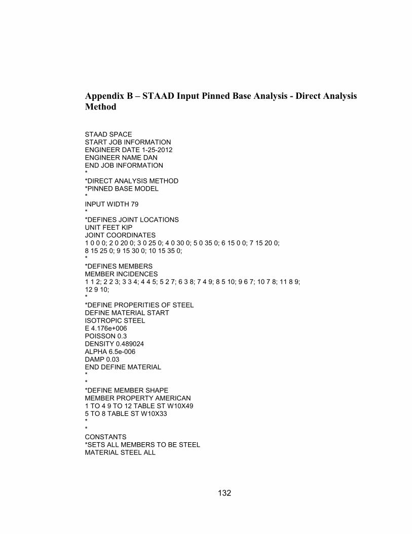
132
Appendix B – STAAD Input Pinned Base Analysis - Direct Analysis Method
STAAD SPACE START JOB INFORMATION ENGINEER DATE 1-25-2012 ENGINEER NAME DAN END JOB INFORMATION * *DIRECT ANALYSIS METHOD *PINNED BASE MODEL * INPUT WIDTH 79 * *DEFINES JOINT LOCATIONS UNIT FEET KIP JOINT COORDINATES 1 0 0 0; 2 0 20 0; 3 0 25 0; 4 0 30 0; 5 0 35 0; 6 15 0 0; 7 15 20 0; 8 15 25 0; 9 15 30 0; 10 15 35 0; * *DEFINES MEMBERS MEMBER INCIDENCES 1 1 2; 2 2 3; 3 3 4; 4 4 5; 5 2 7; 6 3 8; 7 4 9; 8 5 10; 9 6 7; 10 7 8; 11 8 9; 12 9 10; * *DEFINE PROPERITIES OF STEEL DEFINE MATERIAL START ISOTROPIC STEEL E 4.176e+006 POISSON 0.3 DENSITY 0.489024 ALPHA 6.5e-006 DAMP 0.03 END DEFINE MATERIAL * * *DEFINE MEMBER SHAPE MEMBER PROPERTY AMERICAN 1 TO 4 9 TO 12 TABLE ST W10X49 5 TO 8 TABLE ST W10X33 * * CONSTANTS *SETS ALL MEMBERS TO BE STEEL MATERIAL STEEL ALL

133
* *DEFINES SUPPORT CONDITIONS SUPPORTS 1 6 PINNED 2 TO 5 7 TO 10 FIXED BUT FX FY MX MY MZ * DEFINE DIRECT ANALYSIS FYLD 7200 ALL FLEX 1 ALL AXIAL ALL NOTIONAL LOAD FACTOR 0.002 END *DEFINES WIND VELOCITY PRESSURE QZ FOR APPLICATION DEFINE WIND LOAD TYPE 1 INT 0.02127 0.02127 0.02252 0.02352 0.02452 0.02602 HEIG 0 15 20 25 30 40 * * * ********************************** *PRIMARY LOAD CASES ********************************** * LOAD 1 DEAD LOAD (DS) STEEL AND FIREPROOFING *SELFWEIGHT OF THE STRUCTURE PLUS 10% FOR CONNECTIONS SELFWEIGHT Y -1.1 * * * * LOAD 2 OPERATING DEAD LOAD (DO) *40 PSF UNIFORM LOAD OVER TRIBUTARY AREA *40PSF*20FEET = 800 PLF = 0.8 KLF MEMBER LOAD 5 TO 8 UNI GY -0.8 * * * LOAD 3 EMPTY DEAD LOAD (DE) *60% OF OPERATING DEAD LOAD MEMBER LOAD 5 TO 8 UNI GY -0.48 * * * LOAD 4 TEST DEAD LOAD (DT) *40 PSF UNIFORM LOAD OVER TRIBUTARY AREA *40PSF*20FEET = 800 PLF = 0.8 KLF MEMBER LOAD

134
5 TO 8 UNI GY -0.8 * * * LOAD 5 WIND LOAD X DIRECTION (WX) *APPLIES PRESSURE GRADIENT TO MEMBERS IN MODEL, *FACTOR = (GUST * SHAPE FACTOR) *G = 0.85, CD = 2.0 *WIND LOAD ON STRUCTURAL MEMBERS *APPLIED BASED ON PROJECTED AREA WIND LOAD X 1.7 TYPE 1 OPEN *WIND ON PIPE OR CABLE TRAY JOINT LOAD 2 7 FX 0.371 3 8 FX 0.387 4 9 FX 0.404 5 10 FX 0.429 * * * LOAD 7 SEISMIC LOAD X DIRECTION (EX) *SEISMIC LOAD APPLIED BASED ON VERTICAL DISTRIBUTION JOINT LOAD 2 7 FX 0.475 3 8 FX 0.725 4 9 FX 1.05 5 10 FX 1.425 * * * LOAD 14 SEISMIC LOAD Y DIRECTION (EY) *PRIMARY LOADS 1 AND 2 MULTIPLIED BY 10% *LOAD 1 DEAD LOAD (DS) STEEL AND FIREPROOFING SELFWEIGHT Y -0.11 * *LOAD 2 OPERATING DEAD LOAD (DO) MEMBER LOAD 5 TO 8 UNI GY -0.08 * * * LOAD 9 PIPE FRICTION LOAD (FF) *10% OF OPERATING DEAD LOAD APPLIED LONGITUDINAL MEMBER LOAD 5 TO 8 UNI GZ 0.08 * * * LOAD 10 PIPE ANCHOR LOAD (AF) *5% OF OPERATING DEAD LOAD APPLIED TRANSVERSE

135
MEMBER LOAD 5 TO 8 UNI GX 0.04 * * * LOAD 11 THERMAL EXPANSION FORCE (T) *DELTA T OF 0 DEGREES APPLIED TO ALL STRUCTURAL MEMBERS TEMPERATURE LOAD 1 TO 12 TEMP 0 * * * LOAD 15 NOTIONAL LOAD (N) *LOAD 1 AND 2 MULTIPLIED BY 0.002 AND APPLIED LATERALLY *LOAD 1 DEAD LOAD (DS) STEEL AND FIREPROOFING *SELFWEIGHT OF THE STRUCTURE PLUS 10% FOR CONNECTIONS SELFWEIGHT X 0.0022 * *LOAD 2 OPERATING DEAD LOAD (DO) *40 PSF UNIFORM LOAD OVER TRIBUTARY AREA *40PSF*20FEET = 800 PLF = 0.8 KLF MEMBER LOAD 5 TO 8 UNI GX 0.0016 * * LOAD 20 NATURAL PERIOD CALCULATION *LOAD 1 DEAD LOAD (DS) STEEL AND FIREPROOFING SELFWEIGHT x -1.1 *LOAD 2 OPERATING DEAD LOAD (DO) MEMBER LOAD 5 TO 8 UNI Gx -0.8 *LOAD 3 EMPTY DEAD LOAD (DE) MEMBER LOAD 5 TO 8 UNI Gx -0.48 modal calculation requested * * ************************************************** * ASD LOAD COMBINATIONS ************************************************** * DS+DO+FF+T+AF+L+S ************************************************** LOAD 101 DS+DO+FF+T+AF REPEAT LOAD 1 1.0 2 1.0 9 1.0 11 1.0 10 1.0 * LOAD 102 DS+DO-FF+T-AF REPEAT LOAD 1 1.0 2 1.0 9 -1.0 11 1.0 10 -1.0 *

136
LOAD 103 DS+DO+FF-T+AF REPEAT LOAD 1 1.0 2 1.0 9 1.0 11 -1.0 10 1.0 * LOAD 104 DS+DO-FF-T-AF REPEAT LOAD 1 1.0 2 1.0 9 -1.0 11 -1.0 10 -1.0 * ************************************************** * DS+DO+AF+W ************************************************** LOAD 105 DS+DO+AF+WX REPEAT LOAD 1 1.0 2 1.0 10 1.0 5 1.0 * LOAD 106 DS+DO-AF+WX REPEAT LOAD 1 1.0 2 1.0 10 -1.0 5 1.0 * LOAD 107 DS+DO+AF-WX REPEAT LOAD 1 1.0 2 1.0 10 1.0 5 -1.0 * LOAD 108 DS+DO-AF-WX REPEAT LOAD 1 1.0 2 1.0 10 -1.0 5 -1.0 * ************************************************** * DS+DO+AF+0.7E ************************************************** LOAD 109 DS+DO+AF+0.7EX+0.7EY REPEAT LOAD 1 1.0 2 1.0 10 1.0 7 0.7 14 0.7 * LOAD 110 DS+DO-AF+0.7EX+0.7EY REPEAT LOAD 1 1.0 2 1.0 10 -1.0 7 0.7 14 0.7 * LOAD 111 DS+DO+AF-0.7EX+0.7EY REPEAT LOAD 1 1.0 2 1.0 10 1.0 7 -0.7 14 0.7 * LOAD 112 DS+DO-AF-0.7EX+0.7EY REPEAT LOAD 1 1.0 2 1.0 10 -1.0 7 -0.7 14 0.7 * ************************************************** * DS+DE+W ************************************************** LOAD 113 DS+DE+WX
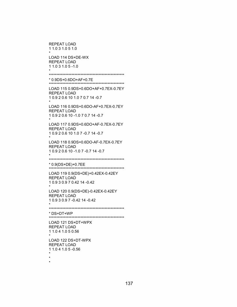
137
REPEAT LOAD 1 1.0 3 1.0 5 1.0 * LOAD 114 DS+DE-WX REPEAT LOAD 1 1.0 3 1.0 5 -1.0 * ************************************************** * 0.9DS+0.6DO+AF+0.7E ************************************************** LOAD 115 0.9DS+0.6DO+AF+0.7EX-0.7EY REPEAT LOAD 1 0.9 2 0.6 10 1.0 7 0.7 14 -0.7 * LOAD 116 0.9DS+0.6DO-AF+0.7EX-0.7EY REPEAT LOAD 1 0.9 2 0.6 10 -1.0 7 0.7 14 -0.7 * LOAD 117 0.9DS+0.6DO+AF-0.7EX-0.7EY REPEAT LOAD 1 0.9 2 0.6 10 1.0 7 -0.7 14 -0.7 * LOAD 118 0.9DS+0.6DO-AF-0.7EX-0.7EY REPEAT LOAD 1 0.9 2 0.6 10 -1.0 7 -0.7 14 -0.7 * ************************************************** * 0.9(DS+DE)+0.7EE ************************************************** LOAD 119 0.9(DS+DE)+0.42EX-0.42EY REPEAT LOAD 1 0.9 3 0.9 7 0.42 14 -0.42 * LOAD 120 0.9(DS+DE)-0.42EX-0.42EY REPEAT LOAD 1 0.9 3 0.9 7 -0.42 14 -0.42 * ************************************************** * DS+DT+WP ************************************************** LOAD 121 DS+DT+WPX REPEAT LOAD 1 1.0 4 1.0 5 0.56 * LOAD 122 DS+DT-WPX REPEAT LOAD 1 1.0 4 1.0 5 -0.56 * * *
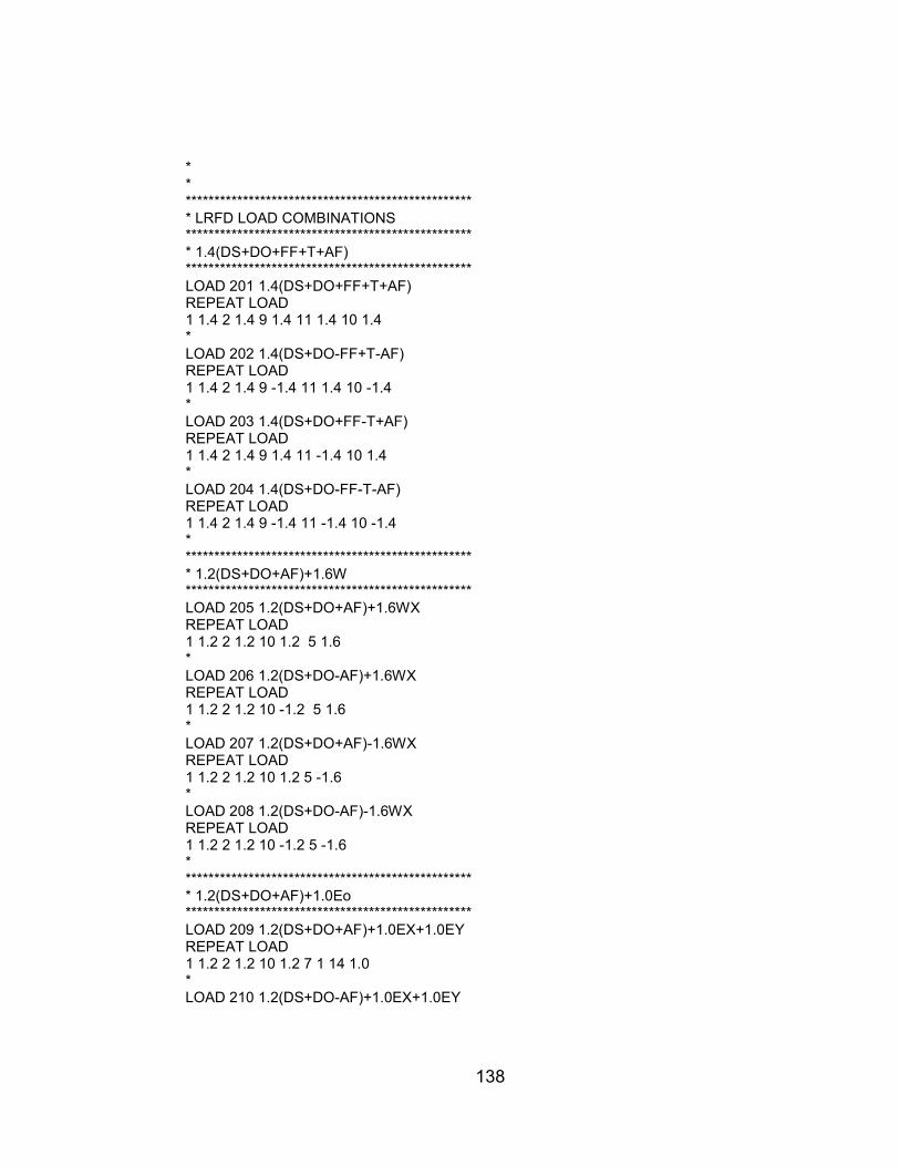
138
* * ************************************************** * LRFD LOAD COMBINATIONS ************************************************** * 1.4(DS+DO+FF+T+AF) ************************************************** LOAD 201 1.4(DS+DO+FF+T+AF) REPEAT LOAD 1 1.4 2 1.4 9 1.4 11 1.4 10 1.4 * LOAD 202 1.4(DS+DO-FF+T-AF) REPEAT LOAD 1 1.4 2 1.4 9 -1.4 11 1.4 10 -1.4 * LOAD 203 1.4(DS+DO+FF-T+AF) REPEAT LOAD 1 1.4 2 1.4 9 1.4 11 -1.4 10 1.4 * LOAD 204 1.4(DS+DO-FF-T-AF) REPEAT LOAD 1 1.4 2 1.4 9 -1.4 11 -1.4 10 -1.4 * ************************************************** * 1.2(DS+DO+AF)+1.6W ************************************************** LOAD 205 1.2(DS+DO+AF)+1.6WX REPEAT LOAD 1 1.2 2 1.2 10 1.2 5 1.6 * LOAD 206 1.2(DS+DO-AF)+1.6WX REPEAT LOAD 1 1.2 2 1.2 10 -1.2 5 1.6 * LOAD 207 1.2(DS+DO+AF)-1.6WX REPEAT LOAD 1 1.2 2 1.2 10 1.2 5 -1.6 * LOAD 208 1.2(DS+DO-AF)-1.6WX REPEAT LOAD 1 1.2 2 1.2 10 -1.2 5 -1.6 * ************************************************** * 1.2(DS+DO+AF)+1.0Eo ************************************************** LOAD 209 1.2(DS+DO+AF)+1.0EX+1.0EY REPEAT LOAD 1 1.2 2 1.2 10 1.2 7 1 14 1.0 * LOAD 210 1.2(DS+DO-AF)+1.0EX+1.0EY

139
REPEAT LOAD 1 1.2 2 1.2 10 -1.2 7 1 14 1.0 * LOAD 211 1.2(DS+DO+AF)-1.0EX+1.0EY REPEAT LOAD 1 1.2 2 1.2 10 1.2 7 -1.0 14 1.0 * LOAD 212 1.2(DS+DO-AF)-1.0EX+1.0EY REPEAT LOAD 1 1.2 2 1.2 10 -1.2 7 -1.0 14 1.0 * ************************************************** * 0.9(DE+DE)+1.6W ************************************************** LOAD 213 0.9(DS+DE)+1.6WX REPEAT LOAD 1 0.9 3 0.9 5 1.6 * LOAD 214 0.9(DS+DE)-1.6WX REPEAT LOAD 1 0.9 3 0.9 5 -1.6 * ************************************************** * 0.9(DS+DO)+1.2AF+1.0E ************************************************** LOAD 215 0.9(DS+DO)+1.2AF+EX-EY REPEAT LOAD 1 0.9 2 0.9 10 1.2 7 1.0 14 -1.0 * LOAD 216 0.9(DS+DO)-1.2AF+EX-EY REPEAT LOAD 1 0.9 2 0.9 10 -1.2 7 1.0 14 -1.0 * LOAD 217 0.9(DS+DO)+1.2AF-EX-EY REPEAT LOAD 1 0.9 2 0.9 10 1.2 7 -1.0 14 -1.0 * LOAD 218 0.9(DS+DO)-1.2AF-EX-EY REPEAT LOAD 1 0.9 2 0.9 10 -1.2 7 -1.0 14 -1.0 * ************************************************** * 0.9(DS+DE)+1.0EE ************************************************** LOAD 219 0.9(DS+DE)+EEX-EEY REPEAT LOAD 1 0.9 3 0.9 7 0.6 14 -0.6 * LOAD 220 0.9(DS+DE)-EEX-EEY REPEAT LOAD

140
1 0.9 3 0.9 7 -0.6 14 -0.6 * ************************************************** * 1.4(DS+DT) ************************************************** LOAD 221 1.4(DS+DT+NX) REPEAT LOAD 1 1.4 4 1.4 * LOAD 222 1.4(DS+DT-NX) REPEAT LOAD 1 1.4 4 1.4 * ************************************************** * 1.2(DS+DT)+1.6(0.56W) ************************************************** LOAD 223 1.2(DS+DT)+1.6(0.56WX) REPEAT LOAD 1 1.2 4 1.2 5 0.9 * LOAD 224 1.2(DS+DT)-1.6(0.56WX) REPEAT LOAD 1 1.2 4 1.2 5 -0.9 * * * PERFORM DIRECT ANALYSIS LRFD ITERATION 10 TAUTOL 0.01 DISPTOL 1e-014 LOAD LIST 201 TO 224 PARAMETER 1 CODE AISC UNIFIED FYLD 7200 ALL * KZ 1 ALL KY 1 ALL * CHECK CODE ALL * FINISH

141
Appendix C – STAAD Input Pinned Base Analysis - First Order Method STAAD SPACE START JOB INFORMATION ENGINEER DATE 1-25-2012 ENGINEER NAME DAN END JOB INFORMATION * *FIRST ORDER METHOD *PINNED BASE MODEL * INPUT WIDTH 79 * *DEFINES JOINT LOCATIONS UNIT FEET KIP JOINT COORDINATES 1 0 0 0; 2 0 20 0; 3 0 25 0; 4 0 30 0; 5 0 35 0; 6 15 0 0; 7 15 20 0; 8 15 25 0; 9 15 30 0; 10 15 35 0; * *DEFINES MEMBERS MEMBER INCIDENCES 1 1 2; 2 2 3; 3 3 4; 4 4 5; 5 2 7; 6 3 8; 7 4 9; 8 5 10; 9 6 7; 10 7 8; 11 8 9; 12 9 10; * *DEFINE PROPERITIES OF STEEL DEFINE MATERIAL START ISOTROPIC STEEL E 4.176e+006 POISSON 0.3 DENSITY 0.489024 ALPHA 6.5e-006 DAMP 0.03 END DEFINE MATERIAL * * *DEFINE MEMBER SHAPE MEMBER PROPERTY AMERICAN 1 TO 4 9 TO 12 TABLE ST W10X49 5 TO 8 TABLE ST W10X33 * * CONSTANTS *SETS ALL MEMBERS TO BE STEEL MATERIAL STEEL ALL *
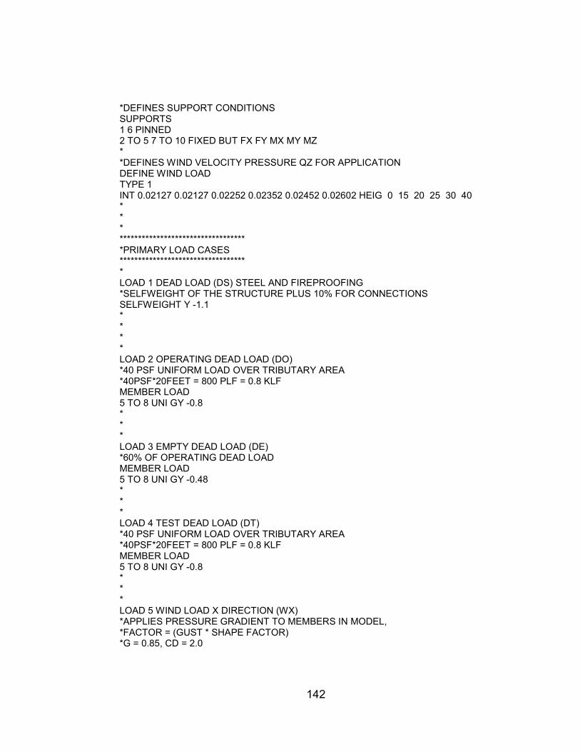
142
*DEFINES SUPPORT CONDITIONS SUPPORTS 1 6 PINNED 2 TO 5 7 TO 10 FIXED BUT FX FY MX MY MZ * *DEFINES WIND VELOCITY PRESSURE QZ FOR APPLICATION DEFINE WIND LOAD TYPE 1 INT 0.02127 0.02127 0.02252 0.02352 0.02452 0.02602 HEIG 0 15 20 25 30 40 * * * ********************************** *PRIMARY LOAD CASES ********************************** * LOAD 1 DEAD LOAD (DS) STEEL AND FIREPROOFING *SELFWEIGHT OF THE STRUCTURE PLUS 10% FOR CONNECTIONS SELFWEIGHT Y -1.1 * * * * LOAD 2 OPERATING DEAD LOAD (DO) *40 PSF UNIFORM LOAD OVER TRIBUTARY AREA *40PSF*20FEET = 800 PLF = 0.8 KLF MEMBER LOAD 5 TO 8 UNI GY -0.8 * * * LOAD 3 EMPTY DEAD LOAD (DE) *60% OF OPERATING DEAD LOAD MEMBER LOAD 5 TO 8 UNI GY -0.48 * * * LOAD 4 TEST DEAD LOAD (DT) *40 PSF UNIFORM LOAD OVER TRIBUTARY AREA *40PSF*20FEET = 800 PLF = 0.8 KLF MEMBER LOAD 5 TO 8 UNI GY -0.8 * * * LOAD 5 WIND LOAD X DIRECTION (WX) *APPLIES PRESSURE GRADIENT TO MEMBERS IN MODEL, *FACTOR = (GUST * SHAPE FACTOR) *G = 0.85, CD = 2.0

143
*WIND LOAD ON STRUCTURAL MEMBERS *APPLIED BASED ON PROJECTED AREA WIND LOAD X 1.7 TYPE 1 OPEN *WIND ON PIPE OR CABLE TRAY JOINT LOAD 2 7 FX 0.371 3 8 FX 0.387 4 9 FX 0.404 5 10 FX 0.429 * * * LOAD 7 SEISMIC LOAD X DIRECTION (EX) *SEISMIC LOAD APPLIED BASED ON VERTICAL DISTRIBUTION JOINT LOAD 2 7 FX 0.475 3 8 FX 0.725 4 9 FX 1.05 5 10 FX 1.425 * * * LOAD 14 SEISMIC LOAD Y DIRECTION (EY) *PRIMARY LOADS 1 AND 2 MULTIPLIED BY 10% *LOAD 1 DEAD LOAD (DS) STEEL AND FIREPROOFING SELFWEIGHT Y -0.11 * *LOAD 2 OPERATING DEAD LOAD (DO) MEMBER LOAD 5 TO 8 UNI GY -0.08 * * * LOAD 9 PIPE FRICTION LOAD (FF) *10% OF OPERATING DEAD LOAD APPLIED LONGITUDINAL MEMBER LOAD 5 TO 8 UNI GZ 0.08 * * * LOAD 10 PIPE ANCHOR LOAD (AF) *5% OF OPERATING DEAD LOAD APPLIED TRANSVERSE MEMBER LOAD 5 TO 8 UNI GX 0.04 * * * LOAD 11 THERMAL EXPANSION FORCE (T) *DELTA T OF 0 DEGREES APPLIED TO ALL STRUCTURAL MEMBERS TEMPERATURE LOAD

144
1 TO 12 TEMP 0 * * * LOAD 15 NOTIONAL LOAD (N) *LOAD 1 AND 2 MULTIPLIED BY 0.0323 AND APPLIED LATERALLY *BASED ON 1/DELTA = 65 *LOAD 1 DEAD LOAD (DS) STEEL AND FIREPROOFING *SELFWEIGHT OF THE STRUCTURE PLUS 10% FOR CONNECTIONS SELFWEIGHT X 0.03553 * *LOAD 2 OPERATING DEAD LOAD (DO) *40 PSF UNIFORM LOAD OVER TRIBUTARY AREA *40PSF*20FEET = 800 PLF = 0.8 KLF MEMBER LOAD 5 TO 8 UNI GX 0.02584 * * LOAD 20 NATURAL PERIOD CALCULATION *LOAD 1 DEAD LOAD (DS) STEEL AND FIREPROOFING SELFWEIGHT x -1.1 *LOAD 2 OPERATING DEAD LOAD (DO) MEMBER LOAD 5 TO 8 UNI Gx -0.8 *LOAD 3 EMPTY DEAD LOAD (DE) MEMBER LOAD 5 TO 8 UNI Gx -0.48 modal calculation requested * * ************************************************** * ASD LOAD COMBINATIONS ************************************************** * DS+DO+FF+T+AF ************************************************** LOAD COMB 101 DS+DO+FF+T+AF 1 1.0 2 1.0 9 1.0 11 1.0 10 1.0 * LOAD COMB 102 DS+DO-FF+T-AF 1 1.0 2 1.0 9 -1.0 11 1.0 10 -1.0 * LOAD COMB 103 DS+DO+FF-T+AF 1 1.0 2 1.0 9 1.0 11 -1.0 10 1.0 * LOAD COMB 104 DS+DO-FF-T-AF 1 1.0 2 1.0 9 -1.0 11 -1.0 10 -1.0 * ************************************************** * DS+DO+AF+W **************************************************
145
LOAD COMB 105 DS+DO+AF+WX 1 1.0 2 1.0 10 1.0 5 1.0 * LOAD COMB 106 DS+DO-AF+WX 1 1.0 2 1.0 10 -1.0 5 1.0 * LOAD COMB 107 DS+DO+AF-WX 1 1.0 2 1.0 10 1.0 5 -1.0 * LOAD COMB 108 DS+DO-AF-WX 1 1.0 2 1.0 10 -1.0 5 -1.0 * ************************************************** * DS+DO+AF+0.7E ************************************************** LOAD COMB 109 DS+DO+AF+0.7EX+0.7EY 1 1.0 2 1.0 10 1.0 7 0.7 14 0.7 * LOAD COMB 110 DS+DO-AF+0.7EX+0.7EY 1 1.0 2 1.0 10 -1.0 7 0.7 14 0.7 * LOAD COMB 111 DS+DO+AF-0.7EX+0.7EY 1 1.0 2 1.0 10 1.0 7 -0.7 14 0.7 * LOAD COMB 112 DS+DO-AF-0.7EX+0.7EY 1 1.0 2 1.0 10 -1.0 7 -0.7 14 0.7 * ************************************************** * DS+DE+W ************************************************** LOAD COMB 113 DS+DE+WX 1 1.0 3 1.0 5 1.0 * LOAD COMB 114 DS+DE-WX 1 1.0 3 1.0 5 -1.0 * ************************************************** * 0.9DS+0.6DO+AF+0.7E ************************************************** LOAD COMB 115 0.9DS+0.6DO+AF+0.7EX-0.7EY 1 0.9 2 0.6 10 1.0 7 0.7 14 -0.7 * LOAD COMB 116 0.9DS+0.6DO-AF+0.7EX-0.7EY 1 0.9 2 0.6 10 -1.0 7 0.7 14 -0.7 * LOAD COMB 117 0.9DS+0.6DO+AF-0.7EX-0.7EY 1 0.9 2 0.6 10 1.0 7 -0.7 14 -0.7 * LOAD COMB 118 0.9DS+0.6DO-AF-0.7EX-0.7EY 1 0.9 2 0.6 10 -1.0 7 -0.7 14 -0.7

146
* ************************************************** * 0.9(DS+DE)+0.7EE ************************************************** LOAD COMB 119 0.9(DS+DE)+0.42EX-0.42EY 1 0.9 3 0.9 7 0.42 14 -0.42 * LOAD COMB 120 0.9(DS+DE)-0.42EX-0.42EY 1 0.9 3 0.9 7 -0.42 14 -0.42 * ************************************************** * DS+DT+WP ************************************************** LOAD COMB 121 DS+DT+WPX 1 1.0 4 1.0 5 0.56 * LOAD COMB 122 DS+DT-WPX 1 1.0 4 1.0 5 -0.56 * * * ************************************************** * LRFD LOAD COMBINATIONS (WITH NOTIONAL) ************************************************** * 1.4(DS+DO+FF+T+AF) ************************************************** LOAD COMB 201 1.4(DS+DO+FF+T+AF+NX) 1 1.4 2 1.4 9 1.4 11 1.4 10 1.4 15 1.4 * LOAD COMB 202 1.4(DS+DO-FF+T-AF-NX) 1 1.4 2 1.4 9 -1.4 11 1.4 10 -1.4 15 -1.4 * LOAD COMB 203 1.4(DS+DO+FF-T+AF+NX) 1 1.4 2 1.4 9 1.4 11 -1.4 10 1.4 15 1.4 * LOAD COMB 204 1.4(DS+DO-FF-T-AF-NX) 1 1.4 2 1.4 9 -1.4 11 -1.4 10 -1.4 15 -1.4 * ************************************************** * 1.2(DS+DO+AF)+1.6W ************************************************** LOAD COMB 205 1.2(DS+DO+AF+NX)+1.6WX 1 1.2 2 1.2 10 1.2 5 1.6 15 1.2 * LOAD COMB 206 1.2(DS+DO-AF+NX)+1.6WX 1 1.2 2 1.2 10 -1.2 5 1.6 15 1.2 * LOAD COMB 207 1.2(DS+DO+AF-NX)-1.6WX 1 1.2 2 1.2 10 1.2 5 -1.6 15 -1.2 *

147
LOAD COMB 208 1.2(DS+DO-AF-NX)-1.6WX 1 1.2 2 1.2 10 -1.2 5 -1.6 15 -1.2 * LOAD COMB 209 1.2(DS+DO+AF-NX)+1.6WX 1 1.2 2 1.2 10 1.2 5 1.6 15 -1.2 * LOAD COMB 210 1.2(DS+DO-AF-NX)+1.6WX 1 1.2 2 1.2 10 -1.2 5 1.6 15 1.2 * LOAD COMB 211 1.2(DS+DO+AF+NX)-1.6WX 1 1.2 2 1.2 10 1.2 5 -1.6 15 1.2 * LOAD COMB 212 1.2(DS+DO-AF+NX)-1.6WX 1 1.2 2 1.2 10 -1.2 5 -1.6 15 1.2 * ************************************************** * 1.2(DS+DO+AF)+1.0Eo ************************************************** LOAD COMB 213 1.2(DS+DO+AF+NX)+1.0EX+1.0EY 1 1.2 2 1.2 10 1.2 7 1 14 1.0 15 1.2 * LOAD COMB 214 1.2(DS+DO-AF+NX)+1.0EX+1.0EY 1 1.2 2 1.2 10 -1.2 7 1 14 1.0 15 1.2 * LOAD COMB 215 1.2(DS+DO+AF+NX)-1.0EX+1.0EY 1 1.2 2 1.2 10 1.2 7 -1.0 14 1.0 15 1.2 * LOAD COMB 216 1.2(DS+DO-AF+NX)-1.0EX+1.0EY 1 1.2 2 1.2 10 -1.2 7 -1.0 14 1.0 15 1.2 * LOAD COMB 217 1.2(DS+DO+AF-NX)+1.0EX+1.0EY 1 1.2 2 1.2 10 1.2 7 1 14 1.0 15 -1.2 * LOAD COMB 218 1.2(DS+DO-AF-NX)+1.0EX+1.0EY 1 1.2 2 1.2 10 -1.2 7 1 14 1.0 15 -1.2 * LOAD COMB 219 1.2(DS+DO+AF-NX)-1.0EX+1.0EY 1 1.2 2 1.2 10 1.2 7 -1.0 14 1.0 15 -1.2 * LOAD COMB 220 1.2(DS+DO-AF-NX)-1.0EX+1.0EY 1 1.2 2 1.2 10 -1.2 7 -1.0 14 1.0 15 -1.2 * ************************************************** * 0.9(DE+DE)+1.6W ************************************************** LOAD COMB 221 0.9(DS+DE+NX)+1.6WX 1 0.9 3 0.9 5 1.6 15 0.9 * LOAD COMB 222 0.9(DS+DE-NX)-1.6WX 1 0.9 3 0.9 5 -1.6 15 -0.9

148
* ************************************************** * 0.9(DS+DO)+1.2AF+1.0E ************************************************** LOAD COMB 223 0.9(DS+DO+NX)+1.2AF+EX-EY 1 0.9 2 0.9 10 1.2 7 1.0 14 -1.0 15 0.9 * LOAD COMB 224 0.9(DS+DO+NX)-1.2AF+EX-EY 1 0.9 2 0.9 10 -1.2 7 1.0 14 -1.0 15 0.9 * LOAD COMB 225 0.9(DS+DO+NX)+1.2AF-EX-EY 1 0.9 2 0.9 10 1.2 7 -1.0 14 -1.0 15 0.9 * LOAD COMB 226 0.9(DS+DO+NX)-1.2AF-EX-EY 1 0.9 2 0.9 10 -1.2 7 -1.0 14 -1.0 15 0.9 * LOAD COMB 227 0.9(DS+DO-NX)+1.2AF+EX-EY 1 0.9 2 0.9 10 1.2 7 1.0 14 -1.0 15 -0.9 * LOAD COMB 228 0.9(DS+DO-NX)-1.2AF+EX-EY 1 0.9 2 0.9 10 -1.2 7 1.0 14 -1.0 15 -0.9 * LOAD COMB 229 0.9(DS+DO-NX)+1.2AF-EX-EY 1 0.9 2 0.9 10 1.2 7 -1.0 14 -1.0 15 -0.9 * LOAD COMB 230 0.9(DS+DO-NX)-1.2AF-EX-EY 1 0.9 2 0.9 10 -1.2 7 -1.0 14 -1.0 15 -0.9 * ************************************************** * 0.9(DS+DE)+1.0E ************************************************** LOAD COMB 231 0.9(DS+DE+NX)+EEX-EEY 1 0.9 3 0.9 7 0.6 14 -0.6 15 0.9 * LOAD COMB 232 0.9(DS+DE-NX)-EEX-EEY 1 0.9 3 0.9 7 -0.6 14 -0.6 15 -0.9 * ************************************************** * 1.4(DS+DT) ************************************************** LOAD COMB 233 1.4(DS+DT+NX) 1 1.4 4 1.4 15 1.4 * LOAD COMB 234 1.4(DS+DT-NX) 1 1.4 4 1.4 15 1.4 * ************************************************** * 1.2(DS+DT)+1.6(0.56W) ************************************************** LOAD COMB 235 1.2(DS+DT+NX)+1.6(0.56WX)

149
1 1.2 4 1.2 5 0.9 15 1.2 * LOAD COMB 236 1.2(DS+DT-NX)-1.6(0.56WX) 1 1.2 4 1.2 5 -0.9 15 -1.2 * * * * PERFORM ANALYSIS LOAD LIST 201 TO 236 PARAMETER 1 CODE AISC UNIFIED FYLD 7200 ALL * KZ 1 ALL KY 1 ALL * CHECK CODE ALL * FINISH
Related Documents