SQL in the Clouds - Western Washington University

12 This arTicle has been peer-reviewed. Computing in SCienCe & engineering

C l o u dC o m p u t i n g

T he distinguishing features of a cloud computing environment are a large collection of inexpensive, off-the-shelf commodity processors and a

generic interconnection network. No customized components address reliability, computational speed, or network efficiency. Instead, a redundant system dynamically circumvents failures, bottle-necks, and imbalances. Each node’s data files, for example, have replicas throughout the system, and periodic comparisons maintain data existence and integrity across isolated failures. Processor components are also under surveillance; the sys-tem addresses a slow or nonfunctional node by lightening its workload or moving it entirely to other nodes. Invisible to the cloud user, this infra-structure maintenance ensures a stable, reliable, and massively parallel computing engine.

Internet information companies, notably Google, have successfully deployed large cloud computing systems for which their applications seem particularly well suited. Maintaining search-engine query histories and attaining petabyte

sizes, Web logs, for example, are systematically mined for patterns that inform crucial business decisions. Many inquiries against such data take a select-group-aggregate form, such as “Find queries subsequent to January 1, 2008, contain-ing the word ‘car’ or ‘automobile,’ and count them by state.” The user expects answers such as “Ken-tucky 4,538,006” and similar entries for other states. To explore such data mining operations in a cloud computing context, Google evolved a cloud adaptation of the MapReduce algorithm, based on primitives long available in Lisp. In pro-posing solutions for select-group-aggregate data mining requests, however, the MapReduce approach enters competition with traditional da-tabase management systems. SQL is the premier data-extraction language of relational databases, and select-group-aggregate extractions cor-respond to a popular SQL template. The auto-mobile example might appear in SQL as

select state, count(∗) as carCountfrom queryLog

where queryDate > ‘2008.01.01’groupby state

Research efforts have produced several data mining languages, each purporting to implement a cloud computing solution for certain SQL con-

Exploring algorithms that exploit cloud computing’s inherent dataflow nature reveals that a few customizable templates, assembled recursively as necessary, can handle a wide class of SQL data mining queries.

1521-9615/09/$25.00 © 2009 ieee

CopubliShed by the ieee CS and the aip

James L. JohnsonWestern Washington University

SQL in the Clouds

July/auguSt 2009 13

structions (see the “Related Work in Data Mining Languages” sidebar). Each of these constructions, in turn, attempts to reduce the considerable effort needed to launch a MapReduce job. For select-group-aggregate queries, the map phase selects relevant data from each input record. Because its selection logic involves only fields in a record, the map could, in theory, consider all records simulta-neously. In practice, however, the user apportions the input among a prescribed number of map in-stances through a job configuration specification. Each map then operates serially on its assigned input, emitting keyed tuples for grouping by a systemwide sort. The sorted output proceeds to a bank of reduce jobs, all running in parallel, each performing the final aggregation for some key’s

subset. In general, both the map and reduce phas-es execute arbitrary code, subject only to some general formatting constraints. This complexity contrasts sharply with SQL, where simple syntax embeds certain application identifiers and con-stants, as in the automobile example.

The appearance of these languages has provoked a lively debate in the database management com-munity. Prominent players have suggested that the cloud approach offers no new functionality and ignores years of accumulated best practices. Nevertheless, Google presents a persuasive proof of concept in its restricted application domain. Moreover, several commercial software vendors have announced cloud database undertakings, such as the Sun Microsystems Drizzle project (www.h-

Related WoRk in data Mining languages

Several data mining languages purport to implement a cloud computing solution for certain SQL construc-

tions, each attempting to reduce the effort needed to launch a MapReduce job.

Google’s proprietary software, both its distributed file system1 and its Bigtable relational overlay,2 have open source equivalents in the Apache-supported Hadoop3 project. Both use the MapReduce algorithm, and both find writing code for the parallel map and reduce phases to be a tedious and error-prone task. Consequently, both evolved scripting languages to capture query intent and produce MapReduce code automatically. In a Google Sawzall4 script, concise filter and aggregate syntax generate, respectively, map and reduce code. The Hadoop counterpart, Pig-Latin,5 acknowledges SQL’s influence on an inventory of impera-tive transformations that compile into MapReduce code. With both languages, the user must manually reconstruct nonprocedural SQL as a data-transformation sequence suit-able for eventual MapReduce implementation. Simple SQL queries admit such manipulation; more complex queries don’t. Among its transformations, Pig-Latin achieves SQL joins, but neither supports correlated subqueries.

Accepting certain SQL syntax almost verbatim and sup-porting both inner and outer relational joins, Microsoft’s Structure Computations Optimized for Parallel Execution (Scope) language6 nevertheless precludes subqueries. However, by cleverly exploiting outer joins and redefining SQL’s standard treatment of null values, Scope attains some results SQL typically reaches through subqueries. Such indirect subquery support requires programmer inter-vention to reconstruct the SQL as a data-transformation sequence in an imperative script subset of the language.

In the main text, I elaborate two SQL-query classes useful in data mining, the distinguishing feature being whether or not the query, expressed in the predicate calculus, requires universal quantifiers or their negated existential equivalents. If so, a relational algebra solution uses division operations, and well-known equivalent expressions achieve the same result with joins and set differences alone; if not, a subquery-free SQL solution typically exists.7 Scope offers a combine operation that executes user-defined code on tuple collections and should therefore easily support set operations. Consequently, it appears that Scope can reach the level of SQL expressions this article promotes, albeit with imperative script programs rather than nonprocedural SQL syntax.

ReferencesS. Ghemawat et al., “The Google File System,” 1. Proc. 19th ACM

Symp. Operating System Principles (SOSP 03), ACM Press, 2003, pp.

29–43.

F. Chang et al., “Bigtable: A Distributed Storage System for 2.

Structured Data,” Proc. 7th Usenix Symp. Operating Systems Design

and Implementation (OSDI 06), Usenix Assoc., 2006, pp. 205–218.

D. Borthakur, 3. The Hadoop Distributed File System: Architecture and

Design, Apache Software Foundation; http://hadoop.apache.org/

core/docs/r0.16.4/hdfs_design.html.

R. Pike et al., “Interpreting the Data: Parallel Analysis with Sawzall,” 4.

Scientific Programming, vol. 13, no. 4, 2005, pp. 277–298.

C. Olston et al., “Pig-Latin: A Not-So-Foreign Language for Data 5.

Processing,” Proc. ACM SIGMOD Int’l Conf. Management of Data

(SIGMOD 08), ACM Press, 2008, pp. 1099–1110.

R. Chaiken et al., “SCOPE: Easy and Efficient Parallel Processing of 6.

Massive Data Sets,” Proc. Int’l Conf. Very Large Data Bases (VLDB

08), Very Large Data Base Endowment, 2008, pp. 1265–1276.

J.L. Johnson, 7. Database: Models, Languages, Design, Oxford Univ.

Press, 1997.

14 Computing in SCienCe & engineering

online.com/news/Drizzle-a-MySQL-fork-for-web -applications--/111154). I take no position in this controversy. Rather, in this article, I suggest al-gorithms that exploit a computing cloud’s inher-ent dataflow nature to solve a broad range of SQL data-mining queries. In particular, I emphasize a pattern that interlaces elementary but massively parallel cloud computations with systemwide sorting and redistribution of results. To the ex-tent possible, the heavy lifting occurs in the sort-ing and redistribution phases, which constitute a generic service available to all queries. In the end, algorithm performance will depend on this redis-tribution process’s efficiency.

This effort is worthwhile because SQL is a widely recognized standard for specifying how to extract desired information from a relational data-base. SQL queries reflect an underlying predicate calculus and consequently provide a powerful tool for expressing the desired extraction. In practice, if the required information is definable with a first-order predicate, a user can express it in SQL.

A Broadly inclusive SQl SubsetI propose a restricted subset of SQL queries,

covering a range of applications and amenable to parallel implementation through cloud comput-ing concepts. Following my textbook’s approach,1 I first examine the predicates underlying a SQL query. In abstract terms, I use SQL to identify database tuples satisfying a predicate. Normally, a user wants to view certain attribute extractions from such tuples, and consequently the SQL ex-pression encodes a set construction, such as {x.a, y.b | P(x, y)}. In this example, free variables x and y range over all tuples in the database, and P is a first-order predicate calculus expression that’s true for the desired tuples. Attributes a and b, ex-tracted from surviving tuples x and y, respectively, constitute the answer set.

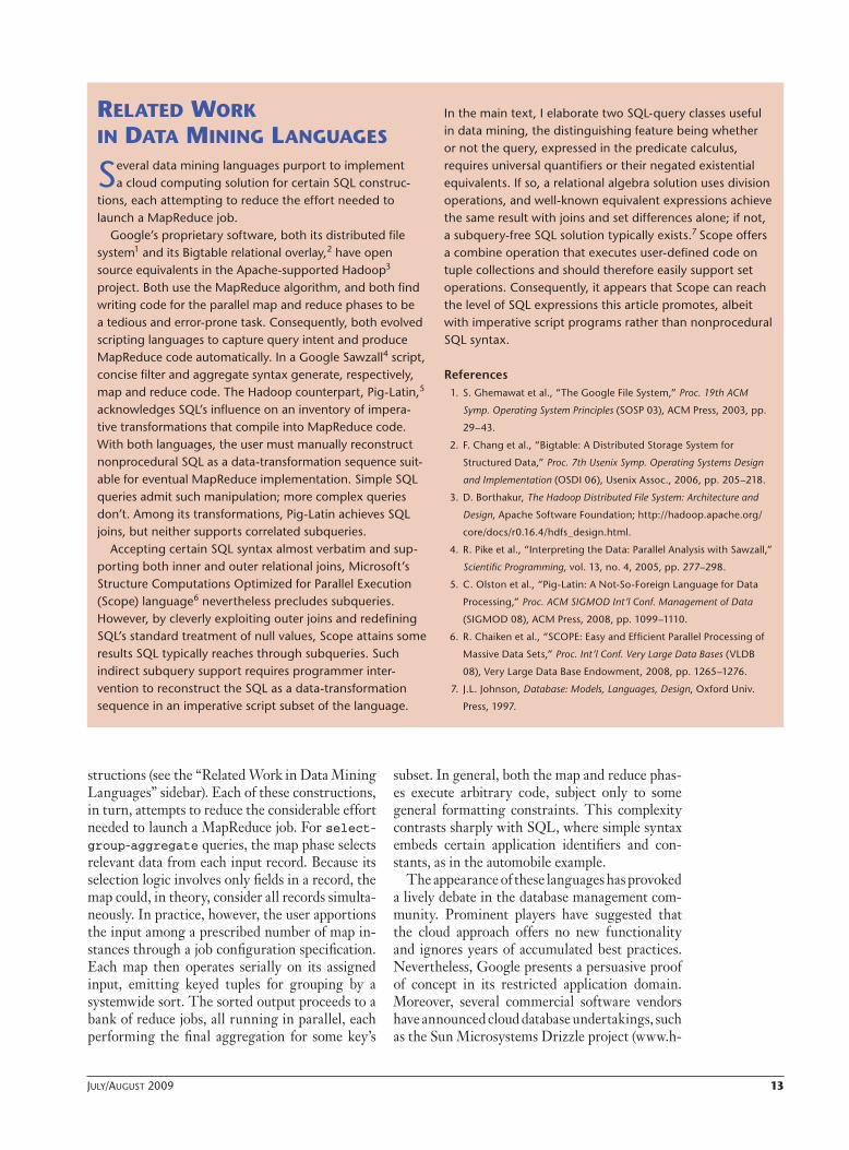
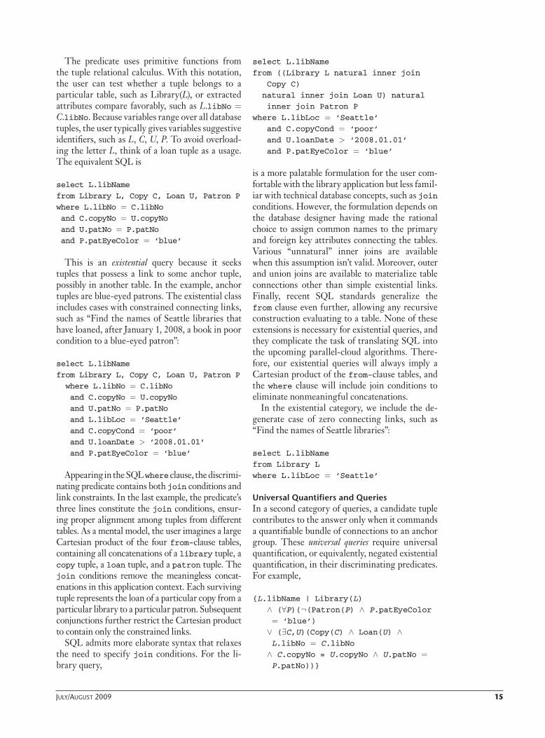
I’ll use a simple database in these examples. De-scribing a library system’s relevant entities, Figure 1 is an abbreviated entity-relationship diagram, a common standard for expressing relational database designs. In this example, four relationships connect the five entities. A library typically holds many books, but to distinguish among a book’s multiple copies, I interpose the Copy entity between Li-brary and Book. A book is now an abstraction; a library or a copy is a physical object. In this context, tuples with the same libNo attribute constitute a meaningful collection, an instance of the one-to-many relationship between Library and Copy, containing exactly one library tuple and zero or more copy tuples. Similar comments apply to the remaining entities. Copies, for example, can partici-pate in many loans, each of which involves a single patron. I developed queries against this database to illustrate that a small number of generic templates covers most of the desired recovery patterns.

Existential Quantifiers and QueriesCategorizing predicates supporting SQL expres-sions first requires distinguishing those involving only nonnegated existential quantifiers. In prac-tice, this constraint means that a tuple contributes to the answer when it has a connection to any one of certain anchor tuples. An example involving only nonnegated existential quantifiers appears in the following query, requesting the names of libraries that loaned a book to a blue-eyed patron. The wedge, ∧, is a logical conjunction; the invert-ed wedge, ∨, is a logical disjunction.

{L.libName | Library(L) ∧ (∃C, U, P) (Copy(C) ∧ Loan(U) ∧ Patron(P) ∧ L.libNo = C.libNo ∧ C.copyNo = U.copyNo ∧ U.patNo = P.patNo ∧ P.patEyeColor = ‘blue’)}

LoanloanNoloanDateloanDuecopyNopatNo

LibrarylibNolibNamelibLoc

BookbookNobookTitlebookPages

CopycopyNocopyDatecopyCondlibNobookNo

PatronpatNopatNamepatEyeColorpatAgepatWeight

Figure 1. Entity-relationship diagram. This abbreviated entity-relationship diagram describes a library system’s relevant entities. The boldfaced entries are primary keys; matching italicized identifiers in other tables constitute foreign keys. The arrows indicate one-to-many relationships, tuple groupings on a common value in the common attribute.

July/auguSt 2009 15

The predicate uses primitive functions from the tuple relational calculus. With this notation, the user can test whether a tuple belongs to a particular table, such as Library(L), or extracted attributes compare favorably, such as L.libNo = C.libNo. Because variables range over all database tuples, the user typically gives variables suggestive identifiers, such as L, C, U, P. To avoid overload-ing the letter L, think of a loan tuple as a usage. The equivalent SQL is

select L.libName

from Library L, Copy C, Loan U, Patron P

where L.libNo = C.libNo and C.copyNo = U.copyNo and U.patNo = P.patNo and P.patEyeColor = ‘blue’

This is an existential query because it seeks tuples that possess a link to some anchor tuple, possibly in another table. In the example, anchor tuples are blue-eyed patrons. The existential class includes cases with constrained connecting links, such as “Find the names of Seattle libraries that have loaned, after January 1, 2008, a book in poor condition to a blue-eyed patron”:

select L.libName

from Library L, Copy C, Loan U, Patron P

where L.libNo = C.libNo and C.copyNo = U.copyNo and U.patNo = P.patNo and L.libLoc = ‘Seattle’ and C.copyCond = ‘poor’ and U.loanDate > ‘2008.01.01’ and P.patEyeColor = ‘blue’

Appearing in the SQL where clause, the discrimi-nating predicate contains both join conditions and link constraints. In the last example, the predicate’s three lines constitute the join conditions, ensur-ing proper alignment among tuples from different tables. As a mental model, the user imagines a large Cartesian product of the four from-clause tables, containing all concatenations of a library tuple, a copy tuple, a loan tuple, and a patron tuple. The join conditions remove the meaningless concat-enations in this application context. Each surviving tuple represents the loan of a particular copy from a particular library to a particular patron. Subsequent conjunctions further restrict the Cartesian product to contain only the constrained links.

SQL admits more elaborate syntax that relaxes the need to specify join conditions. For the li-brary query,

select L.libName

from ((Library L natural inner join

Copy C)

natural inner join Loan U) natural

inner join Patron P

where L.libLoc = ‘Seattle’ and C.copyCond = ‘poor’ and U.loanDate > ‘2008.01.01’ and P.patEyeColor = ‘blue’

is a more palatable formulation for the user com-fortable with the library application but less famil-iar with technical database concepts, such as join conditions. However, the formulation depends on the database designer having made the rational choice to assign common names to the primary and foreign key attributes connecting the tables. Various “unnatural” inner joins are available when this assumption isn’t valid. Moreover, outer and union joins are available to materialize table connections other than simple existential links. Finally, recent SQL standards generalize the from clause even further, allowing any recursive construction evaluating to a table. None of these extensions is necessary for existential queries, and they complicate the task of translating SQL into the upcoming parallel-cloud algorithms. There-fore, our existential queries will always imply a Cartesian product of the from-clause tables, and the where clause will include join conditions to eliminate nonmeaningful concatenations.

In the existential category, we include the de-generate case of zero connecting links, such as “Find the names of Seattle libraries”:

select L.libName

from Library L

where L.libLoc = ‘Seattle’

universal Quantifiers and QueriesIn a second category of queries, a candidate tuple contributes to the answer only when it commands a quantifiable bundle of connections to an anchor group. These universal queries require universal quantification, or equivalently, negated existential quantification, in their discriminating predicates. For example,

{L.libName | Library(L)

∧ (∀P)(¬(Patron(P) ∧ P.patEyeColor = ‘blue’) ∨ (∃C,U)(Copy(C) ∧ Loan(U) ∧ L.libNo = C.libNo ∧ C.copyNo = U.copyNo ∧ U.patNo = P.patNo))}

ritascanlan

Callout

first


requests the names of libraries that have served all blue-eyed patrons. Because SQL quantification is existential by default, we transform the predicate before translating it to the SQL not exists syn-tax, a construction for testing a subquery’s empty status:


∧ ¬(∃P)((Patron(P) ∧ P.patEyeColor = ‘blue’) ∧ ¬(∃C,U)(Copy(C) ∧ Loan(U) ∧ L.libNo = C.libNo ∧ C.copyNo = U.copyNo ∧ U.patNo = P.patNo))}

select L.libName

from Library L

where not exists

(select ∗ from Patron P

where P.patEyeColor = ‘blue’ and not exists

(select ∗ from Copy C, Loan U

where L.libNo = C.libNo and C.copyNo = U.copyNo and U.patNo = P.patNo))

The double negation construction isn’t particu-larly intuitive, so it’s helpful to rephrase the quali-fying condition as “The set of blue-eyed patrons with no connections to the candidate library must be empty.” The SQL syntax constructs certain intermediate tables in the where clause and then tests them for empty content. These intermediate tables constitute SQL subqueries.

It’s always possible that a subquery doesn’t de-pend on the particular candidate tuple under test. This case would arise in the previous example if the subquery construction were independent of the variable L. On occasion this simplification does occur, typically in statements containing multiple subqueries. However, the interesting subqueries are correlated subqueries—subqueries that do depend on the tuple under test and must, in principle, be reconstructed for each such tuple. Convoluted alternative constructions exist in some cases, but the simplest universal-query SQL rendition uses correlated subqueries.

Although correlated subqueries complicate par-allel computation schemes, universal queries are too important to neglect. Entities of interest are often identifiable through their connections to all or to a significant portion of known anchors. For instance, the user might want to know librar-

ies that serve more than 70 percent of the blue-eyed patrons. This variant requires a higher-order predicate calculus expression:


∧ (∃S)(S ∈ ω(Patron) ∧ |S| > 0.7 × |Patron| ∧ (∀P)( ¬(P ∈ S ∧ P.patEyeColor = ‘blue’) ∨ (∃C,U)(Copy(C) ∧ Loan(U) ∧ L.libNo = C.libNo ∧ C.copyNo = U.copyNo ∧ U.patNo = P.patNo)))}

where ω(Patron) denotes the set of all patron tuple subsets, and the notation |S| means the number of tuples in collection S. Current SQL doesn’t support such expressions, specifically those that involve quantification over tuple sub-sets, although the literature reports explorations in this direction.2,3

Nevertheless, SQL admits restricted subset manipulation through a procedural refinement of the query semantics. Ideally SQL would simply be a more user-friendly translation of the underly-ing nonprocedural predicate calculus. However, most SQL users envision a particular processing order—that is, the from clause implies a Carte-sian product, subsequently filtered by the where clause and partitioned on attributes specified in a groupby clause. A having-clause predicate filters the generated equivalence classes, and the final re-sult contains selections from the filtered classes.

This procedural algorithm has two conse-quences. First, it lets a user work with subsets of tuples, the aforementioned equivalence classes. This artifice doesn’t extend SQL to higher-or-der predicate calculus expressions: it enables no quantification over tuple subsets. Rather, it allows procedural manipulation of sets obtained via pre-specified groupings. Second, the answer set must now contain attribute selections from the surviv-ing equivalence classes. Such a selection is either an attribute from the unpartitioned table, which happens to have the same value across all mem-bers of the equivalence class, or an aggregate of some sort over the members. As a boundary case, if the select clause contains an aggregate, but no groupby clause exists, then the entire table (after the where-clause filtration) constitutes one equivalence class.

The groupby and having clauses will find use in later queries. For the moment, the boundary case will more simply locate the libraries that serve all blue-eyed patrons by counting the num-

July/auguSt 2009 17

ber of blue-eyed patrons and comparing the total with the number of blue-eyed patrons reachable from the candidate library. In the solution below, the second subquery correlates with the library under test, although the first doesn’t. Moreover, both subqueries select an aggregate (a count) but specify no groupby clause. Consequently, the count operates over the full table that the where-clause filter delivers. Because each subquery con-structs just one equivalence class, each evaluates to a single tuple containing a single attribute, the count. In this case, SQL overloads arithmetic operators and comparisons, letting the user treat these tables as singleton numbers:

select L.libName

from Library L

where(select count(P.patNo)

from Patron P

where P.patEyeColor = ‘blue’) = (select count(distinct P.patNo)

from Patron P, Loan U, Copy C

where L.libNo = C.libNo and C.copyNo = U.copyNo and U.patNo = P.patNo and P.patEyeColor = ‘blue’)

This flexibility conveniently permits the follow-ing solution to the related query, “Find the names of libraries that serve more than 70 percent of the blue-eyed patrons”:

select L.libName

from Library L

where 0.7 × (select count(P.patNo) from Patron P

where P.patEyeColor = ‘blue’) < (select count(distinct P.patNo)



Incidentally, the “count(distinct P.patNo)” in the second subquery is necessary to avoid over-counting the blue-eyed patrons linked to the candi-date library. The where-clause predicate operates on the Cartesian product of Patron, Loan, and Copy, retaining each concatenation with appro-priate connections among its segments and to the library under test. If a blue-eyed patron borrows several books from the target library, his patNo

occurs multiple times in the filtered result. There-fore, an unqualified count will overcount such patrons, possibly admitting a library that hasn’t covered 70 percent of the blue-eyed patrons.

groupby and Having ClausesI introduced the SQL aggregate feature to devise a more implementation-friendly syntax for univer-sal queries, but the examples to this point haven’t used the groupby and having clauses. However, I do mean to include them in the restricted SQL. As a final example, consider the query, “For li-braries with an average page count per book greater than 500, report the library name and a count of its books.” Here, the assumption is that the user desires an unduplicated count—that is, a library’s multiple copies of a given book don’t increase its book count. Nor do multiple copies affect the average page count, which I take to mean an unweighted average over the books in a library’s collection:

select L.libNo, L.libName, count(∗) as bookCount

from Library L, Book B

where exists (select ∗ from Copy C

where L.libNo = C.libNo and C.bookNo = B.bookNo)groupby L.libNo, L.libName

having average(B.pages) > 500

The logic pairs libraries with their books and then assigns the resulting tuples to equivalence classes, each containing the pairings for a particu-lar library. If the average page count of the books is small, the system discards the class, computing book counts only for the surviving classes. The where-clause subquery operates on the Carte-sian product of Library and Book and retains only those concatenations in which the prefix library holds one or more copies of the suffix book. Consequently, multiple book copies don’t introduce multiple entries in the result that the filtering operation passes to the grouping phase. The latter operation breaks the surviving tuples into groups, one for each library. Because a book appears at most once with a given library, the user can employ the simpler count(∗) to count the books. This syntax simply produces a tuple count for each group.

Using count(distinct B.bookNo) to count the books in a group formed from the filtered Cartesian product of Library, Copy, and Book seems a legitimate way to avoid the subquery.


This simpler strategy worked in the preceding ex-ample but doesn’t here because the having clause commands a more precise computation over the groups. If a group contains library-copy-book concatenations, a given book can appear in mul-tiple tuples, one for each copy the library holds. The average page count computation would then be a weighted average. As this example illustrates, an existential query might also require a subquery when aggregates are involved.

In the translations to cloud dataflows that fol-low, proper input SQL syntax is the user’s assumed responsibility—that is, the user will construct correct SQL, taking into account the nuances I’ve mentioned.

Cloud Computing and the mapReduce AlgorithmMapReduce is the cloud computing environment’s most popular algorithm. Web search companies, needing rapid search response to user queries, pi-oneered this parallel approach to index very large files of essentially immutable data. It appears that they seldom, if ever, entertain a join query and certainly never a universal query of the sort that I’ve described. Their queries typically fall into the existential category, specifically the case in which the linking tuple chain’s length is zero.

The MapReduce algorithm derives from simi-larly named Lisp primitives: the map, transform-ing a function and a list to a new list, and the reduce, transforming a function and a list to a new value:

map( f,(a1, a2, … , an)) → ( f(a1), f (a2), … , f (an))

reduce( f,(a1, a2, … , an)) → f ( f (··· f ( f(a1, a2), a3), … , an)) …)

The map operation clearly invites parallelism because no dependence exists among the func-tional evaluations. Given sufficient processors, an algorithm can safely pursue all n evaluations in parallel. A reduce operation recursively applies its associative, commutative, binary function argu-ment—for example, reduce(×, (2, 5, 3)) = (2 × 5) × 3 = 30. Actually, this particular variant is called foldl in Lisp, as it rolls up the input list from the left side. Parallelism ensues because of the ability to iterate parallel operations on pairs, giving the result in time proportional to the logarithm of the input-list length.

Google’s cloud map is directly analogous to the Lisp map, but its reduce is more general than the Lisp version, allowing an arbitrary list function. Because I introduce variants in the next section,

I refer to Google’s MapReduce as the traditional algorithm. The traditional MapReduce formula-tion accepts a user-defined split of the input data, launches parallel map functions for each segment, collects the map output in groups, and then per-forms parallel reduce actions on each group. A job tracker—the “system” in the following explana-tion—orchestrates these activities.

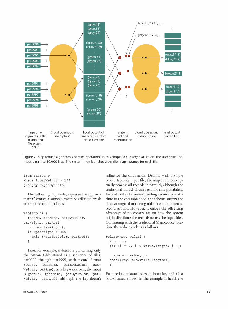
Figure 2 shows the dataflow associated with a simple SQL query evaluation and provides an overview of the MapReduce algorithm. In this al-gorithm, the user first splits the input data into files, and for each file, the system launches a par-allel map instance. Ideally, each map executes on the node where its data file resides. If this optimal allocation isn’t possible, the interconnecting net-work moves data as necessary. Each map accesses its file through a user-defined reader object that presents the data as a sequence of key-value pairs, say (k1, v1)—that is, the reader constructs a pair (k1, v1) from each input line. Typically, both k1 and v1 are strings. The map’s user-specified code con-verts each (k1, v1) into zero, one, or more key-value pairs. Each map output is then a list with elements of the form (k2, v2).

Next, through a configuration file, the user specifies the number of parallel reduce operations, say R, and a corresponding partition of the possible k2 values. That is, a certain subset of k2 keys associ-ates with reducer 1, another disjoint subset with reducer 2, and so forth through an assignment for reducer R. A map instance writes its output to a partitioned file on the local node disk. An output k2 inhabits a partition subset of the possible k2 val-ues, which specifies a reducer target. The target determines the output file segment for the emitted (k2, v2) pair. Upon completing all map instances, the system collects corresponding partition seg-ments across all nodes, sorts these segments on the k2 values, and starts a parallel reduce operation for each of them. Because of the intervening system sort, each reduce instance serially processes inputs of the form (k2, {v2})—that is, a key and its associ-ated value list—and outputs records of the form f(k2, {v2}). The function f indicates a second user-specified function, which executes on all reducers. Finally, the R reduce instances leave R files in the global distributed file system.

More specifically, Figure 2 charts the dataflow paths for the following SQL query, which com-putes the average age of patrons who weigh more than 150 pounds by eye color:

select P.patEyeColor,

average(P.patAge) as avgAge

July/auguSt 2009 19

from Patron P

where P.patWeight > 150groupby P.patEyeColor

The following map code, expressed in approxi-mate C syntax, assumes a tokenize utility to break an input record into fields:

map(input) {

(patNo, patName, patEyeColor,

patWeight, patAge)

= tokenize(input);

if (patWeight > 150) emit ((patEyeColor, patAge));

}

Take, for example, a database containing only the patron table stored as a sequence of files, pat0000 through pat9999, with record format (patNo, patName, patEyeColor, pat-

Weight, patAge). As a key-value pair, the input is (patNo, (patName, patEyeColor, pat-Weight, patAge)), although the key doesn’t

influence the calculation. Dealing with a single record from its input file, the map could concep-tually process all records in parallel, although the traditional model doesn’t exploit this possibility. Instead, with the system feeding records one at a time to the common code, the scheme suffers the disadvantage of not being able to compute across record groups. However, it enjoys the offsetting advantage of no constraints on how the system might distribute the records across the input files. Continuing with the traditional MapReduce solu-tion, the reduce code is as follows:

reduce(key, value) {

sum = 0;

for (i = 0; i < value.length; i++)

sum += value[i];

emit((key, sum/value.length));

}

Each reduce instance sees an input key and a list of associated values. In the example at hand, the

...

...

...

...

...

pat9999

pat9998

pat9997

pat9996

pat9995

...

...

pat0004

pat0003

pat0002

pat0001

pat0000

...

(green,20)(hazel,28)

...

(brown,18)(brown,28)

...

(blue,23)(gray,32)(blue,48)

...

...

(green,41)(green,27)

...

(brown,33)(brown,19)

...

(gray,45)(blue,15)(gray,25)

...

(blue,22.9)

(gray,31.4)

...

blue:15,23,48,

gray:45,25,32,

brown21.1

green31.1

hazel41.2

Input filesegments in the

distributedfile system

(DFS)

Cloud operation: map phase

Local output of two representative

cloud elements

System sort and

redistribution

Cloud operation: reduce phase

Final output in the DFS

Figure 2. MapReduce algorithm’s parallel operation. In this simple SQL query evaluation, the user splits the input data into 10,000 files. The system then launches a parallel map instance for each file.

ritascanlan

Callout

add parens around each entry and commas between the data -- (brown,21.1) ...

ritascanlan

Pencil


key is an eye color, and the list contains the ages of patrons with that eye color. The logic computes the average age by traversing the list as usual, with value[i] addressing the list’s ith entry.

Operating over the 10,000 files in parallel, each map instance emits (patEyeColor, patAge) pairs, such as (blue, 46), storing them in a seg-mented local file. The figure shows blue and gray assigned to one segment and brown assigned to another. When the map phase is complete, each map instance tells the system where its blue-and-gray segment, for example, is located. The system gathers the information, sorts it by eye color, and forwards it to a reducer. The user specifies the number of parallel reducers and consequently the number of segments in each map output.

In this example, the reduce instance associat-ed with the blue-and-gray segment receives two input bundles, which it processes serially. One bundle contains the key “blue” and a list of ages extracted from heavy, blue-eyed patrons; the sec-ond bundle delivers a similar age list for heavy, gray-eyed patrons. The same reduce code executes for both inputs—that is, the two executions could proceed in parallel, although the user has chosen to assign them to the same cloud-processor node. Other reduce instances handle sorted map emis-sions buffered in other map output segments and corresponding to other eye colors.

A more effective data storage format and a vari-ant of the traditional MapReduce algorithm will facilitate the SQL query algorithms in the follow-ing section.

Restricted SQl parallel EvaluationI propose four changes to the data-processing approach of the preceding section. First, I use a special encoding to store all the data in a single Bigtable structure, incorporating some redun-dancy and using the row identifiers to encode information about a tuple’s neighbors in the enti-ty-relationship diagram.

Second, I change how the system distributes map instances, launching a map instance for each Bigtable tablet. The map code is small, as the previous example illustrates, and the tablets are large, typically 100 Mbytes. Consequently, dis-tributing code is more efficient than transferring data. Moreover, a map instance processes only a local data tablet and therefore induces no network data traffic.

Third, I generalize the dataflow to incorpo-rate multiple reduce phases that execute serially. I allow any phase to emit input to a downstream phase through the traditional system sort and re-

distribution. Current practice frequently chains MapReduce jobs, so this modification merely ac-knowledges existing tradition.

Finally, a cloud phase can emit static constant data directly to a subsequent phase, bypassing the normal system-sort activity and propagating to all replicas of the target reduce operation. The traditional MapReduce algorithm employs coun-ter objects, which I didn’t describe in the previ-ous section’s overview; readers familiar with the algorithm’s refinements will recognize the static emissions as similar to these counters.

data Storage FormatGoogle’s Bigtable software provides a large table structure stored on the distributed file system and able to accommodate heterogeneous data. I can store library, copy, book, loan, and patron tuples in a single Bigtable, wasting no storage on null representations for the many missing attri-butes in each tuple. Bigtable stores data units ad-dressable with a row identifier and a column name. Consequently, each tuple comprises a group of rows, each with the same row identifier and con-taining a (column-name, column-data) pair. The group contains as many such rows as tuple attri-bute values. Inapplicable attributes, such as book-Title in the case of a library tuple, simply aren’t among the row groups representing that library. An applicable attribute that happens to be missing receives the same treatment. Moreover, Bigtable’s compression scheme collapses multiple string oc-currences, negating storage implications of re-peated column names. Bigtable maintains its data in 100-Mbyte tablets, any of which can reside on any cloud node.

For the next section’s query evaluation algo-rithms, I assume not only a cloud self-repairing infrastructure but also a Bigtable-like database storage format. For the parallel algorithms’ ben-efit, my Bigtable implementation distributes the database tablets across all nodes, even if the data-base size doesn’t force this dispersion. Finally, the row group representing an application tuple isn’t split across tablets.

In an entity-relationship diagram, the term “child” refers to an entity on the many end of a one-to-many relationship, and “parent” refers to the one end. In our library example, Copy is a child with parents Library and Book. A child entity typically has many more tuples than any of its parents, and relationship groupings (involv-ing one parent tuple and potentially many child tuples) might exhibit widely varying average sizes, depending on the particular parent entity. The

July/auguSt 2009 21

library diagram’s one-to-many relationships sug-gest the smallest tuple counts for the library, book, and patron entities and the largest for the loan entity. The copy entity lies somewhere be-tween the two extremes. A library-copy grouping might be larger, on average, than a book-copy grouping. The former represents copies in the same library; the latter multiple copies of the same book. The expectation is an assumption that a given library typically holds more copies, dis-tributed across many books, than there are copies of any given book across all libraries. The truth of this assumption is arguable, but the point is that the parent that induces larger child collections, on average, merits special treatment.

In Google’s Bigtable format, a patron tuple might appear as

row id: 368; patNo: 48

row id: 368; patName: Joe Smith

row id: 368; patEyeColor: blue

row id: 368; patAge: 46

row id: 368; patWeight: 170

A patron with an unknown eye color, for ex-ample, would have a similar pattern, except the patEyeColor association would be missing. Wasting no storage on null values, this scheme also opens opportunities to add unexpected fields. Encountering a patron record that just happens to contain hair color, the user adds row id:

769; hairColor: brown for that patron with-out any effect on existing computations that use the schema. Hair color is simply missing for most patrons. For a child tuple, the designer can take advantage of this flexibility to include parent attri-butes normally indexed. Specifically, the designer can embed certain discerning parent attributes in selected child tuples to facilitate the SQL query evaluation’s filtering phase. Relational design phi-losophy argues against such inclusions, but the redundancy can enhance performance.

Being a long string (up to 64 Kbytes in the Google documentation), a Bigtable row identifier can encode its tuple’s keys, both primary and for-eign. The topmost levels in the entity-relationship diagram represent nonchild entries, having no foreign keys that would link them to yet higher parents. The following three tuples illustrate the storage format for these entities:

row id: Pxxx; patName: Joe Smith

row id: Pxxx; patEyeColor: blue

row id: Pxxx; patAge: 46

row id: Pxxx; patWeight: 170

row id: Lxxx; libName: Jefferson

row id: Lxxx; libLoc: Seattle

row id: Bxxx; bookTitle: The Forgery

row id: Bxxx; bookPages: 539

The row identifiers encode the primary keys, patNo, libNo, and bookNo, represented as xxx in the example, with the leading letter identify-ing the appropriate table. Now consider the child entity Copy with parents Library and Book. In context, suppose a collection of copies with a given library parent is typically larger than a collection with a given book parent. In this sense, Library is the dominant parent of Copy, a status reflected in the generic Copy record:

row id: L1xxx-Byyy-Czzz;

copyDate: 2006.06.30


copyCond: poor

The key-encoding scheme is essentially the same, except that an “L1” prefix identifies a library. Foreign keys precede the tuple’s primary key in the row identifier, and the dominant parent’s for-eign key is leftmost. Because Bigtable maintains each data tablet in ascending row-identifier order, copy tuples appear grouped by library. Indeed, as the database grows, a tablet eventually comprises copies from a single library. In any case, the num-ber of distinct libraries in a tablet is small, justify-ing the inclusion of discerning library attributes in occasional copy tuples. On each tablet, the sys-tem places these library attributes in the first copy tuple corresponding to that library’s group. This anomalous tuple has the format


copyDate: 2006.06.30


copyCond: poor


libName: Jefferson


libLoc: Seattle

The “L0” prefix sorts this tuple at the begin-ning of the corresponding library group, because other copy tuples in the group have the “L1” pre-fix. In this example, both libName and libLoc are discerning attributes, although in the general case, an entity might contain a small number of discerning attributes, together with a bag of words not amenable to indexing. Only the discerning at-tributes appear in scattered copy tuples, although

ritascanlan

Text Box

//I shortened the book title and library name to fit on one line.//


the library tuple, stored elsewhere in the data structure, holds the complete record.

Some early database products included a physi-cal component in the data definition language, letting a designer specify how parent-child re-cords should cluster in storage. Although modern databases typically leave such placement decisions to the database management software, judicious clustering of related tuples remains an important performance consideration. Nevertheless, there are good reasons for questioning specific cluster-ing schemes; one being that a child entity can have more than one parent. This case prevails in my example, and I can’t simultaneously cluster copies with their libraries and with their books. Except for the case in which a library possesses multiple copies of a book, a library’s copy group refers to distinct books. The upcoming SQL query evalu-ation algorithm doesn’t assume embedded attri-butes from nondominant parents, a situation that forces an additional reduce phase to coordinate such parent-child relationship instances.

The Loan child entity regards Copy as the dom-inant parent. Consequently, a tablet groups loan tuples associated with a common copy parent and installs occasional anomalous loan tuples contain-ing the parent copy’s attributes. Differing only in the table identifiers, the format is analogous to the previous example.

Anomalous tuples before copy and loan group-ings imply a table-maintenance complication. As the number of loans grows, for example, the loans associated with a given copy eventually spill onto another tablet. To retain local access to par-ent tuple attributes, the update process must copy the anomalous tuple into the new tablet. Despite this replication, row identifiers remain unique. A duplicated anomalous loan tuple, for example, contains a new “Uzzz” segment in its row identi-fier, corresponding to a new loan on the new tab-let. Consequently, the full-row identifier remains unique. As a final implementation detail, note that anomalous tuples break with the tradition of dis-joint row-identifier ranges on distinct tablets.

Query Evaluation AlgorithmConsider again the existential query, “Find the names of Seattle libraries that have loaned, after January 1, 2008, a book in poor condition to a blue-eyed patron”:

select distinct L.libName

from Library L, Copy C, Loan U,

Patron P

where L.libNo = C.libNo

and C.copyNo = U.copyNo and U.patNo = P.patNo and L.libLoc = ‘Seattle’ and C.copyCond = ‘poor’ and U.loanDate > ‘2008.01.01’ and P.patEyeColor = ‘blue’

In this SQL solution, I added the keyword “dis-tinct” to the select clause because SQL doesn’t suppress duplicates by default. Although this addi-tion necessitates one more reduce phase than does the unadorned query, it nevertheless seems a more suitable example because the SQL user would likely command the duplicate suppression.

Following traditional heuristics by minimizing join inputs, an SQL interpreter might construct Figure 3’s execution plan for this query. Specifi-cally, filter operations pass only relevant tuples from the database tables to the first level joins, and both filter and join operations trim their out-put tuples, retaining only attributes needed in subsequent stages. Viewed from a cloud-hosted MapReduce context, this plan presents several parallel-evaluation opportunities. The initial map phase operates on database tablets and can there-fore perform all four filters in parallel. Of course, each map instance sees only tuples on its assigned tablet, but the code provides conditional execu-tion paths, tailoring the logic to the data present. A more significant advantage derives from the storage format I discussed in the previous section. In particular, Library is the dominant parent for Copy, and anomalous tuples among the cop-ies provide information about the parent library. The map instance scanning a tablet of copy tuples can filter the copies for copyCond = poor, filter the owning library for libLoc = Seattle, and emit qualifying (copyNo, libName) tuples to the top join in Figure 3. A simple scan delivers the results of the lower-left join.

Unfortunately, the same shortcut isn’t avail-able for the lower-right join because Patron isn’t Loan’s dominant parent. However, this join’s pur-pose is to deliver (copyNo) tuples to the upper join, where each such tuple represents a copy that a blue-eyed patron borrowed during the specified loanDate range. Moreover, knowing that only poor-condition copies will survive the upper join, (copyNo), output shouldn’t flow to the upper join unless it meets this condition. Of course, the SQL plan can’t obtain this information from the Loan or Patron tables and therefore can’t take this op-portunity to reduce the upper join’s work. Howev-er, the cloud system can employ anomalous copy tuples embedded among the loans to do so—that

July/auguSt 2009 23

is, the system can achieve much of the lower-right join functionality by scanning the Loan table. In particular, those map instances that encounter loan tuples on their assigned database tablets can filter the loans for loanDate > 2008.01.01, fil-ter the owning copy for copyCond = poor, and emit qualifying (patNo, copyNo) to a later reduce phase, which will filter patrons for eye color.

The system provides an entire tablet—an input tuple stream sorted on increasing row identifier—to each map instance. This structure contrasts sharply with that of a traditional mapper, which treats each input record in isolation. The follow-ing map code assumes utility functions to read tuples and to extract attributes. Because several reduce phases can follow the mapping phase, the emit instruction contains an initial argument that indicates the proper reduce-phase target. A map instance varies its emissions, depending on the tuple type the tablet delivers. For a copy tuple, it exploits the grouping by library and an initial anomalous tuple’s presence. Library location is available from this initial tuple, which presents the opportunity to bypass the entire copy group if the libLoc attribute isn’t Seattle. Otherwise, the map instance emits the pair (copyNo, lib-Info), provided the copy condition is poor. These emissions proceed directly to the second reduce phase. Figure 4 clarifies the reduce-phase targets. For a patron tuple, the map checks the eye-color attribute and conditionally outputs a pair (patNo, null) to reduce-1. Employing a similar strategy, loan-tuple processing skips the loan group associ-ated with a particular copy, if the copy isn’t a poor one. Otherwise, it checks individual loans for timeliness and outputs (patNo, copyNo). Both of these latter emission types flow to the first reduce phase, which completes the lower-right join in Figure 3.

The following reduce code clarifies this process:

map(tablet) {

while ((t = tablet.getTuple) ! = null) if (t.type == copy) { if (t.anomalous)

skipCopy = (t.libLoc ! = ‘Seattle’);

if (!skipCopy && t.anomalous)

libInfo = t.libName; if (!skipCopy && (t.copyCond == poor))

emit(2, (t.copyNo, libInfo));

}

else if (t.type == patron) {

if (t.patEyeColor == ‘blue’) emit(1, (t.patNo, null));

}

else if (t.type == loan) { if (t.anomalous)

skipLoan = (t.copyCond ! = ‘poor’);

if (!skipLoan && (t.loanDate > ‘2008.01.01’))

emit(1, (t.patNo, t.copyNo));

}

}

Figure 4 provides an overview of the cloud computation phases. The map computes the out-put from the lower-left join in Figure 3 from a copy tuple scan and forwards the (copyNo, lib-Name) results to reduce-2, which computes the top join. Throughout Figure 4 and subsequent data-flow diagrams, italicized attributes denote, some-

Library L Copy C Loan U Patron P

L.libLoc = Seattle C.copyCond = poorU.loanDate >2008.01.01

P.patEyeColor =blue

(libNo, libName) (libNo, copyNo)

(copyNo, patNo)

(patNo)

(copyNo, libName) (copyNo)

libName

join

join join

Figure 3. SQL execution plan for a simple existential query. Viewed from a cloud-hosted MapReduce context, this plan presents several parallel-evaluation opportunities.

Copy

Loan

Patron

map

(patNo, null)

(patNo, copyNo)

(copyNo, libName)

(copyNo, null)

(libName) (libName)

reduce-1

reduce-2

reduce-3

Figure 4. Dataflow diagram for a cloud implementation of Figure 3. The map phase alone achieves the lower-left join in Figure 3, whereas the map in conjunction with reduce-1 computes the lower-right join. Reduce-2 suffices for the upper-join, and reduce-3 exists solely to suppress duplicates in the final answer.


what incompletely, values the appropriate SQL query constraint has filtered. For example, when (copyNo, libName) pairs arrive at the reduce-2 interface, the copyNo identifies a poor-condition copy, and the libName is that of a Seattle library. However, in the (patNo, copyNo) pairs arriving at the reduce-1 interface, only the copyNo rep-resents a poor-condition copy; the patNo might or might not correspond to a blue-eyed patron. Moreover, the copyNo represents a poor-condi-tion copy involved in a timely loan. This status is apparent because these copy numbers derive from a scan of loan tuples, although the italicized no-tation can’t carry all of this information—in this case, because no loan attributes propagate to this dataflow location, leaving nothing to italicize.

My storage format is incapable of completely bypassing the lower-right join in Figure 3, which must deliver (copyNo) values that participate in timely loans to blue-eyed patrons. Instead, the map phase exploits the available anomalous loan tuples to emit (patNo, copyNo) values to reduce-1, where they encounter (patNo, null) values rep-resenting blue-eyed patrons. Because they derive from loan tuples, the copyNo values represent poor-condition copies involved in timely loans. Both tuple streams proceed to reduce-1, which forwards only copyNo values that represent poor-condition copies involved in timely loans to blue-eyed patrons. Reduce-1 recognizes such a copyNo when the same patNo pairs both with that copyNo and with a null payload. Fully qualified (copyNo, null) tuples then flow to reduce-2, where similar logic completes the required top join. Library names satisfying the entire SQL query then flow to reduce-3, which removes duplicates. A library name might appear in the reduce-3 input from a variety of paths, each representing a timely loan of a poor-condition book to a blue-eyed patron. It’s unlikely that the user wants to see this repeti-tion. To eliminate duplicates, the system sends the tuples as a payload vector of identical entries to a reducer operating with the common key. That reducer forwards just one entry downstream.

The reduce codes themselves, even more so than the previous map code, represent extremely concise and simple programs. Following the map phase, a system sort prepares the input for the first reduce phase. The sort orders the collection of (patNo, copyNo) and (patNo, null) pairs by patNo, and consequently, a given reduce-1 in-stance sees a single patNo key and a vector of pay-loads, each a copyNo or a null. Because the null payloads arrived from the Patron table, where patNo is a primary key, at most one null payload

will occur. If the null is present, then all copyNo entries represent timely loans of poor-condition copies to this blue-eyed patron, and reduce-1 for-wards (copyNo, null) emissions to reduce-2, us-ing the upper-code segment’s simple logic.

Each reduce-2 instance sees a copyNo and a payload vector of nulls, among which a single libName entry can appear. Consequently, the code need check for only the nonnull entry and emit its libName, providing at least one other null entry appears. The following reduce code details this logic:

reduce1(key, {value}) {

detect = false; i = 0; while (!detect && (i < value.length))

detect = (value[i++] == null); if (detect)

for (i = 0; i < value.length; i++) if (value[i] ! = null) emit(2, (value[i], null));

}

reduce2(key, value) {

detect = false; i = 0; while (!detect && (i < value.length))

detect = (value[i++] ! = null); if (detect && (value.length > 1)) emit(3, (value[i − 1], null)); }

reduce3(key, value) {

emit(4, (key, null));

}

The final segment above shows the simple logic that removes duplicates. In this case, each re-duce-3 instance sees a libName key and a payload vector of nulls. It emits a single tuple, the key, to a subsequent reduce-4. No reduce-4 phase in this computation means that these reduce-3 emis-sions constitute the existential SQL query’s solu-tion. The concise and simple nature of the map and reduce code segments suggests that most of the computational effort occurs in the interven-ing system sorts and data redistributions. These operations are precisely those in which network bandwidth might pose performance difficulties. Using the cloud model to compute existential SQL queries, however, is conceptually simple.

To confirm that this observation extends to SQL involving subqueries, I’ll explore a univer-

July/auguSt 2009 25

sal query. Consider again the following universal query to find the names of libraries serving all blue-eyed patrons. The following set-comparison template, with minor variations, expresses most universal queries:

select L.libName

from Library L

where (select count(P.patNo)

from Patron P

where P.patEyeColor = ‘blue’) = (select count(distinct P.patNo)



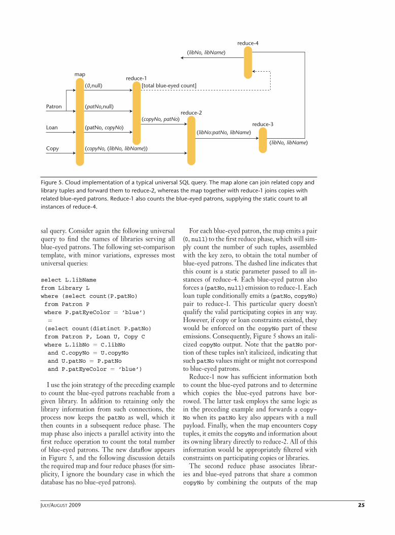
I use the join strategy of the preceding example to count the blue-eyed patrons reachable from a given library. In addition to retaining only the library information from such connections, the process now keeps the patNo as well, which it then counts in a subsequent reduce phase. The map phase also injects a parallel activity into the first reduce operation to count the total number of blue-eyed patrons. The new dataflow appears in Figure 5, and the following discussion details the required map and four reduce phases (for sim-plicity, I ignore the boundary case in which the database has no blue-eyed patrons).

For each blue-eyed patron, the map emits a pair (0, null) to the first reduce phase, which will sim-ply count the number of such tuples, assembled with the key zero, to obtain the total number of blue-eyed patrons. The dashed line indicates that this count is a static parameter passed to all in-stances of reduce-4. Each blue-eyed patron also forces a (patNo, null) emission to reduce-1. Each loan tuple conditionally emits a (patNo, copyNo) pair to reduce-1. This particular query doesn’t qualify the valid participating copies in any way. However, if copy or loan constraints existed, they would be enforced on the copyNo part of these emissions. Consequently, Figure 5 shows an itali-cized copyNo output. Note that the patNo por-tion of these tuples isn’t italicized, indicating that such patNo values might or might not correspond to blue-eyed patrons.

Reduce-1 now has sufficient information both to count the blue-eyed patrons and to determine which copies the blue-eyed patrons have bor-rowed. The latter task employs the same logic as in the preceding example and forwards a copy-No when its patNo key also appears with a null payload. Finally, when the map encounters Copy tuples, it emits the copyNo and information about its owning library directly to reduce-2. All of this information would be appropriately filtered with constraints on participating copies or libraries.

The second reduce phase associates librar-ies and blue-eyed patrons that share a common copyNo by combining the outputs of the map

Copy

Loan

Patron

map

(patNo,null)

(patNo, copyNo)

(copyNo, (libNo, libName))

(copyNo, patNo)

[total blue-eyed count]

(libNo:patNo, libName)

(libNo, libName)

reduce-1

reduce-2

reduce-3

reduce-4

(0,null)

(libNo, libName)

Figure 5. Cloud implementation of a typical universal SQL query. The map alone can join related copy and library tuples and forward them to reduce-2, whereas the map together with reduce-1 joins copies with related blue-eyed patrons. Reduce-1 also counts the blue-eyed patrons, supplying the static count to all instances of reduce-4.


and first reduce phases. Specifically, a reduce-2 instance sees a single copyNo key and a payload vector containing patNo values and one (libNo, libName) entry designating the owning library. Reduce-2 detects the latter entry and treats the rest as a collection of blue-eyed patrons who’ve used this library. Unfortunately, some duplica-tion might occur because a given blue-eyed pa-tron might be connected to this copy through several loans. Consequently, reduce-2 composes emissions of the form (libNo:patNo, libName), which contains a concatenated key.

When reduce-3 sees a key with a long payload vector, it knows it’s receiving duplicates. Reduce-3 passes just one of these values, in the form (libNo, libName) to reduce-4, in which each such entry signals a unique blue-eyed patron for the desig-nated library. Reduce-4 counts these emissions and compares the result with the total number of blue-eyed patrons, received as a static argument from reduce-1. Note that this dataflow extends readily to the related query, “Find the names of libraries that serve more than 70 percent of the blue-eyed patrons.” Reduce-4 simply compares its count with 0.7 times the static parameter.

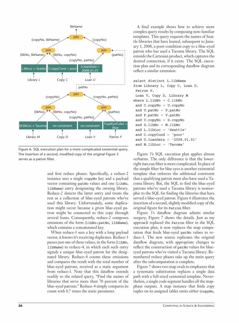
A final example shows how to achieve more complex query results by composing now-familiar templates. This query requests the names of Seat-tle libraries that have loaned, subsequent to Janu-ary 1, 2008, a poor-condition copy to a blue-eyed patron who has used a Tacoma library. The SQL extends the Cartesian product, which captures the desired connection, if it exists. The SQL execu-tion plan and its corresponding dataflow diagram reflect a similar extension:

select distinct L.libName

from Library L, Copy C, Loan U,

Patron P,

Loan V, Copy D, Library M

where L.libNo = C.libNo and C.copyNo = U.copyNo and U.patNo = P.patNo and P.patNo = V.patNo and V.copyNo = D.copyNo and D.libNo = M.libNo and L.libLoc = ‘Seattle’ and C.copyCond = ‘poor’ and U.loanData < ‘2008.01.01’ and M.libLoc = ‘Tacoma’

Figure 3’s SQL execution plan applies almost verbatim. The only difference is that the lower-right Patron filter is more complicated. In place of the simple filter for blue eyes is another existential template that enforces the additional constraint that a qualifying patron must also have used a Ta-coma library. But, the SQL to find the blue-eyed patrons who’ve used a Tacoma library is isomor-phic to the SQL for finding the libraries that have served a blue-eyed patron. Figure 6 illustrates the insertion of a second, slightly modified copy of the original figure for its Patron filter.

Figure 3’s dataflow diagram admits similar surgery; Figure 7 shows the details. Just as my approach replaced the Patron filter in the SQL execution plan, it now replaces the map compu-tation that feeds blue-eyed patNo values to re-duce-1. The new source replicates the original dataflow diagram, with appropriate changes to reflect the construction of patNo values for blue-eyed patrons who’ve visited a Tacoma library. Re-numbered reduce phases take up the main query after the subcomputation is complete.

Figure 7 shows two map ovals to emphasize that a systematic substitution replaces a single data path with a full-sized existential template. Never-theless, a single code segment handles all the map-phase outputs. A map instance that finds copy tuples on its assigned tablet emits either (copyNo,

Library L Copy C Loan U

patNo

L.libLoc = Seattle C.copyCond = poorU.loanDate >2008.01.01

(libNo, libName) (libNo, copyNo)

(copyNo, patNo)

(patNo)

(copyNo, libName) (copyNo)

libName

join

join join

Library M Copy D Loan V Patron P

M.libLoc = Tacoma no constraint no constraintP.patEyeColor =

blue

(libNo) (libNo, copyNo)

(copyNo, patNo)

(patNo)

join

join join

(copyNo) (copyNo, patNo)

Figure 6. SQL execution plan for a more complicated existential query. The insertion of a second, modified copy of the original Figure 3 serves as a patron filter.

July/auguSt 2009 27

libName) tuples to reduce-5, when the owning library is in Seattle, or (copyNo, null) tuples to reduce-2, when the owning library is in Tacoma. In either case, an anomalous tuple provides the needed library location information, and the code maintains two state elements to enable skipping entire copy groups that belong to libraries in nei-ther Seattle nor Tacoma. On patron tuples, the map activity remains unchanged.

The system must still filter patron tuples for eye color, but the output now streams to the new-ly inserted subsidiary dataflow at the top of Fig-ure 7. Only after this subcomputation confirms that the patNo represents a blue-eyed patron of a Tacoma library does the flow return to its origi-nal destination, now relabeled as reduce-4. On loans, the map emits (patNo, copyNo) tuples to reduce-4, if the copy condition is poor and the loan is timely. It also unconditionally emits these tuples to reduce-1 because neither Copy D nor Loan V is subject to a filter. Employing logic that I’ve already analyzed, the six reduce phases com-plete join computations by recognizing payload vectors containing two kinds of inputs and by suppressing duplicates.

This example illustrates how to embed an ex-istential dataflow inside another of the same kind to compose a cloud solution for those queries that qualify a candidate tuple via a longer existential path. SQL from clauses with a large number of tables signal this kind of complexity. However,

similar reasoning holds for other combinations. To find the names of Seattle libraries that have loaned, subsequent to January 1, 2008, a poor-condition copy to a blue-eyed patron who has visited fewer than 50 percent of the Tacoma li-braries, we can substitute a suitably modified universal template, such as that of Figure 5, for the (patNo, null) input to reduce-1. This cut-and-paste procedure embeds a universal template inside a larger existential one. Although space considerations preclude further examples here, it’s clear that I can assemble these two templates in a various combinations to achieve wide cover-age of SQL queries.

T his method’s true worth lies in how it scales to very large databases. It’s here that I should attend the criticism of the traditional database community,

which in pursuit of performance, has accumulated decades of wisdom. For example, the approach I advocate seems to need no indexes because the cloud can see the entire database at once.

In my examples, the map delivers only filtered tuples to the subsequent reduce phases because the SQL constraints apply at the individual table level. This fortuitous happenstance isn’t the most gen-eral case, which means that a large portion of the database might participate in the dataflow. This volume, in turn, implies high network traffic and

Copy D

Loan V

Patron P

map

(patNo, null)

(patNo, copyNo)

(copyNo, libName)

(copyNo, patNo)

(patNo, null) (patNo, null)

reduce-1

reduce-2

reduce-3

Copy C

Loan U

map

(patNo, copyNo)

(copyNo, libName)

(copyNo, null)

(libName) (libName)

reduce-4

reduce-5

reduce-6

Figure 7. Cloud implementation of Figure 6. This dataflow diagram includes renumbered reduce phases to take up the main query after the upper subcomputation.


slower system sorts between reduce phases, both of which negatively impact performance. Even with table-level constraints to throttle map-phase emissions, joins in a subsequent reduce phase might encounter very large data volumes. In the fi rst existential example, all poor-condition cop-ies from Seattle libraries proceed to reduce-2 in search of a matching poor-condition copy involved in a timely loan to a blue-eyed patron. The match-detection logic is trivial; nevertheless, a distinct reduce instance handles each copyNo from either source. In a sense, isn’t this reindexing, anew with each query, an information stream on copyNo? Might some innovative indexing technique exist, suitably structured to exploit the cloud’s architec-tural strengths, to address this problem?

Traditional database research has also developed a large body of theory and practice in construct-ing SQL execution plans. After parsing the input SQL and confi rming its syntactical correctness, the typical SQL engine constructs an execution plan, which it then optimizes for data movement, speed, and size. This process results in a proce-

dural plan, which transforms raw database input in stages to evolve the desired result. These plans correspond roughly to the trees in Figures 3 and 6, but the resemblance is only superfi cial. Where the execution plans in my examples use only the sim-plest heuristics to push selections and projection to the leaves, a commercial-strength optimizer explores a large inventory of rewrite rules to re-structure the initial execution tree. Of particular interest are techniques that enable advantageous subquery elimination. Although this optimization theory is complex and some methods remain pro-prietary to database management vendors, Hec-tor Garcia-Molina and his colleagues’ database text provides an accessible introduction.4 Might similar transformations apply to execution plans targeted to a cloud architecture?

Having an appropriately optimized execution plan, the SQL engine then considers several physi-cal plans, which further identify specifi c algorithms for the procedural steps. The datafl ow diagrams in Figures 4, 5, and 6 are analogous to such plans. To choose a particular plan from many competi-tors, the SQL engine uses database metaknowl-edge: current table sizes, clustering and blocking parameters, the number of tuples with a common value in a specifi ed attribute, the existence of in-dices, and the locations of tuple collections on the network. My research hasn’t considered any of these factors. Here, I’ve simply written straight-forward algorithms that relegate the heavy work to the intervening system sorts. Might there be some method for tuning these algorithms based on metaknowledge of the database?

Although I demonstrate here that SQL evalu-ation in a cloud environment is possible, further study remains to determine if high performance evaluation is achievable.

ReferencesJ.L. Johnson, 1. Database: Models, Languages, Design, Oxford Univ. Press, 1997.

C. Germaine et al., “Online Estimation for Subset-Based SQL 2. Queries,” VLDB J., vol. 16, no. 1, 2007, pp. 745–756.

S.R. Valluri and K. Karlapalem, 3. Subset Queries in Relational Databases, tech. report TR 2003-1, Univ. Augsburg, 2004; http://arxiv.org/ftp/cs/papers/0406/0406029.pdf.

H. Garcia-Molina, J.D. Ullman, and J. Widom, 4. Database Systems: The Complete Book, 2nd ed., Prentice-Hall, 2008.

James l. Johnson is professor of computer science at Western Washington University. His research inter-ests include databases and probabilistic methods in computing. Johnson has a PhD in mathematics from the University of Minnesota. Contact him at [email protected].

Learn about computing history and the people who shaped it.

COMPUTING THEN

http://computingnow.computer.org/ct

SQL in the Clouds - Western Washington University

Documents