Spreading speeds and traveling waves for periodic evolution systems

Spreading Speeds and Traveling Waves

for Periodic Evolution Systems

Xing Liang∗

Department of Mathematics

University of Science and Technology of China

Hefei, Anhui 230026, P. R. China

E-mail: [email protected]

Yingfei Yi†

School of Mathematics

Georgia Institute of Technology

Atlanta, GA 30332-0160, USA

E-mail: [email protected]

Xiao-Qiang Zhao‡

Department of Mathematics and Statistics

Memorial University of Newfoundland

St. John’s, NL A1C 5S7, Canada

E-mail: [email protected]

Abstract The theory of spreading speeds and traveling waves for monotone

autonomous semiflows is extended to periodic semiflows in the monostable case.

∗Research supported in part by the NSF of China.†Research supported in part by the NSF of USA grant DMS0204119.‡Research supported in part by the NSERC of Canada and the MITACS of Canada.

1

Then these abstract results are applied to a periodic system modeling man-

environment-man epidemics, a periodic time-delayed and diffusive equation, and

a periodic reaction-diffusion equation on a cylinder.

Key words and phrases: Monotone systems, spreading speeds, periodic

traveling waves.

2000 Math Subject Classification: 37C65, 37B55, 35K57, 35R10, 92D25

Short title for page headings: Spreading Speeds and Periodic Waves

1 Introduction

There have been extensive investigations on traveling waves and the asymp-

totic (long-time) behavior in terms of asymptotic speeds of spread for various

evolution systems arising in applied sciences, see, e.g., [1]–[4], [6], [10]–[13],

[18]–[20], [22]–[26], [29] and references therein. Asymptotic speed of spread (in

short, spreading speed) was first introduced by Aronson and Weinberger [2] for

reaction-diffusion equations. This concept has proved to be very important in

the study of biological invasions and disease spread. There is an intuitive inter-

pretation for the spreading speed c∗ in a spatial epidemic model: if one runs at

a speed c > c∗, then one will leave the epidemic behind; whereas if one runs at a

speed c < c∗, then one will eventually be surrounded by the epidemic. Recently,

the theory of asymptotic speeds of spread and traveling waves for monotone

semiflows has been developed by Liang and Zhao [11] in such a way that it can

be applied to various autonomous evolution equations admitting the comparison

principle.

It is well known that interactive populations often live in a fluctuating envi-

ronment. For example, physical environmental conditions such as temperature

and humidity and the availability of food, water, and other resources usually

vary in time with seasonal or daily variations. Therefore, more realistic models

should be nonautonomous systems. In particular, if the data in a model are

periodic functions of time with commensurate period, a periodic system arises;

2

if these periodic functions have different (minimal) periods, we get an almost

periodic system. There are a few results on traveling waves for such systems:

Alikakos, Bates and Chen [1], Bates and Chen [3], and Shen [20] established the

existence and global stability of periodic traveling waves for periodic local, non-

local and lattice equations with bistable nonlinearities, respectively; Shen [18]

and Chen [6] also discussed almost periodic traveling waves for almost periodic

local and nonlocal equations in the bistable case; and Shen [19] showed, among

other things, the existence of a family of almost automorphic traveling waves for

a class of almost periodic KPP-type reaction-diffusion equations. However, it

seems that there are at present no exact results for asymptotic speeds of spread

for periodic and almost periodic evolution systems with monostable nonlineari-

ties. Our purpose in the current paper is to study spreading speeds and periodic

traveling waves for monotone periodic semiflows in the monostable case and to

apply the obtained results to three types of periodic evolution systems. Our

results show that the spreading speed coincides with the minimal speed for

monotone periodic traveling waves under reasonable assumptions.

Our approach is to apply the abstract results of [11] on monotone operators

to the Poincare (period) map associated with a given periodic semiflow. We

should also point out that in the case of the continuous spatial habitat, the com-

pactness of the operator with respect to the compact open topology is needed

for the existence of traveling waves in [11] (see also [24, 10]). We will show that

this compactness condition can be replaced with a much weaker one: the map

is a contraction with respect to the Kuratowski measure of noncompactness

(see Remarks 2.1 and 2.3). This new observation makes the developed theory

applicable to some evolution systems consisting of reaction-diffusion equations

coupled with ordinary differential equations (see, e.g., section 3).

The organization of this paper is as follows. In section 2, we summarize the

abstract results for monotone maps (Theorems A, B, C and D) based on [11]. In

order to weaken the compactness condition in [11], we present some properties

of the Kuratowski measure of noncompactness on a Banach space (Lemma 2.1)

and prove the asymptotic precompactness of a sequence of sets associated with

3

the monotone map (Lemma 2.2). Then we show the existence of spreading speed

(Theorem 2.1) for a monotone periodic semiflow, and its coincidence with the

minimal wave speed for monotone periodic traveling waves (Theorems 2.2 and

2.3). In the rest of the paper we apply the general results of section 2 to three

types of periodic differential systems: in section 3 to a periodic system modeling

man-environment-man epidemics; in section 4 to a periodic time-delayed and

diffusive equation; and in section 5 to a periodic reaction-diffusion equation on

a cylinder.

2 Periodic semiflows

Let (X, ‖ · ‖) be a Banach space over R or C. For a bounded subset B of X , the

Kuratowski measure of noncompactness of B is defined as

α(B) = inf r > 0 : B has a finite cover of diameter ≤ r .

Let B be covered by a finite number of subsets M1, · · · ,Mm of X each with

diameter ≤ r. Then B = ∪mi=1(Mi ∩ B) with the diameter of Mi ∩ B ≤ r.

Thus, in the definition of α(B), we can always assume that each set in the finite

cover is a subset of B. For various properties of the Kuratowski measure of

noncompactness, we refer to [14]. The following lemma is a generalization of

[14, Lemma I.5.3]. For the completeness, we provide a proof of it below.

Lemma 2.1. Let d be the distance induced by the norm ‖ · ‖ on X. For two

bounded subsets A,B of X, denote δ(B,A) := supx∈B d(x,A). Let An∞n=1 be

a non-increasing family of non-empty, bounded and closed subsets (i.e., m ≥ n

implies Am ⊂ An). Assume that α(An) → 0 as n → +∞. Then A∞ =⋂

n≥1

An

is non-empty and compact, and δ(An, A∞) → 0 as n→ +∞.

Proof. Given a sequence of points xn with xn ∈ An, ∀n ≥ 1. Since

α(xnn≥1) = α(xnn≥m) ≤ α(Am) → 0, as m→ ∞,

we have α(xnn≥1) = 0. It follows that xn : n ≥ 1 is compact, and hence

xn has a convergent subsequence. Since each An is nonempty, we can choose

4

a sequence of points yn ∈ An. It follows that there is a subsequence nk →∞ such that lim

k→∞ynk

= y0. Thus, the closedness and monotonicity of An

imply that y0 ∈ A∞, and hence A∞ 6= ∅. Clearly, A∞ is closed. Given a

sequence of points zn ⊂ A∞, we have zn ∈ An, ∀n ≥ 1. By what we have

proved, zn has a convergent subsequence. So A∞ is compact. Assume, by

contradiction, that limn→∞

δ(An, A∞) 6= 0. Then there exist a number ε0 > 0, a

sequence of integers mk → ∞, and a sequence of points wmk∈ Amk

such that

d(wmk, A∞) ≥ ε0 for all k ≥ 1. Again by what we have proved, without loss of

generality, we may assume that limk→∞

wmk= w0. Then we have w0 ∈ A∞, and

hence limk→∞

d(wmk, A∞) = d(w0, A∞) = 0, a contradiction.

Let τ be a nonnegative real number and C be the set of all bounded and

continuous functions from [−τ, 0] ×H to Rk, where H = R or Z. Clearly, any

vector in Rk and any element in the Banach space C := C([−τ, 0],Rk) can be

regarded as the functions in C.

For u = (u1, · · · , uk), v = (v1, · · · , vk) ∈ C, we write u ≥ v(u v) provided

ui(θ, x) ≥ vi(θ, x)(ui(θ, x) > vi(θ, x)), ∀i = 1, · · · k, θ ∈ [−τ, 0], x ∈ H; and

u > v provided u ≥ v but u 6= v. For any two vectors a, b in Rk or two functions

a, b ∈ C, we can define a ≥ (>,) b similarly. For any r ∈ C with r 0, we

define Cr := u ∈ C : r ≥ u ≥ 0 and Cr := u ∈ C : r ≥ u ≥ 0.We equip C with the maximum norm topology and C with the compact open

topology, that is, vn → v in C means that the sequence of functions vn(θ, x)

converges to v(θ, x) uniformly for (θ, x) in every compact set. Moreover, we can

define the metric function d(·, ·) in C with respect to this topology by

d(u, v) =

∞∑

k=1

max|x|≤k,θ∈[−τ,0]

|u(θ, x) − v(θ, x)|

2k, ∀u, v ∈ C

such that (C, d) is a metric space.

Define the reflection operator R by R[u](θ, x) = u(θ,−x). Given y ∈ H,

define the translation operator Ty by Ty[u](θ, x) = u(θ, x− y).

Let β ∈ C with β 0 and Q = (Q1, · · · , Qk) : Cβ → Cβ. Assume that

(A1) Q[R[u]] = R[Q[u]], Ty[Q[u]] = Q[Ty[u]], ∀y ∈ H.

5

(A2) Q : Cβ → Cβ is continuous with respect to the compact open topology.

(A3) One of the following two properties holds:

(a) Q[u](·, x) : u ∈ Cβ, x ∈ H is a family of equicontinuous functions

of θ ∈ [−τ, 0].

(b) There is a nonnegative number ς < τ such that Q = S + L, where

S[u](θ, x) =

u(0, x),−τ ≤ θ < −ςQ[u](θ, x),−ς ≤ θ ≤ 0,

is a continuous operator on Cβ and S[u](·, x) : u ∈ Cβ , x ∈ H is a

family of equicontinuous functions of θ ∈ [−τ, 0], and

L[u](θ, x) =

u(θ + ς, x) − u(0, x),−τ ≤ θ < −ς0,−ς ≤ θ ≤ 0.

(A4) Q : Cβ → Cβ is monotone (order-preserving) in the sense that Q[u] ≥ Q[v]

whenever u ≥ v in Cβ.

(A5) Q : Cβ → Cβ admits exactly two fixed points 0 and β, and for any positive

number ε, there is α ∈ Cβ with ‖α‖ < ε such that Qn[α] → β and Q[α] α.

Theorem A. ([11, Theorems 2.11 and 2.15 and Corollary 2.16]) Suppose that

Q satisfies (A1)-(A5). Let u0 ∈ Cβ and un = Q[un−1] for n ≥ 1. Then there is

a real number c∗ such that the following statements are valid:

(1) For any c > c∗, if 0 ≤ u0 β and u0(·, x) = 0 for x outside a bounded

interval, then limn→∞,|x|≥nc

un(θ, x) = 0 uniformly for θ ∈ [−τ, 0].

(2) For any c < c∗ and any σ ∈ Cβ with σ 0, there exists rσ > 0 such that if

u0(·, x) ≥ σ(·) for x on an interval of length 2rσ, then limn→∞,|x|≤nc

un(θ, x) =

β(θ) uniformly for θ ∈ [−τ, 0]. If, in addition, Q is subhomogeneous on

Cβ, then rσ can be chosen to be independent of σ 0.

6

Remark 2.1. Note that the assumption (A3)(a) is equivalent to that the set

Q[u](·, x) : u ∈ Cβ , x ∈ H is precompact in C. In the case where Q has the

translation invariance property in (A1), we have Ty[Cβ] = Cβ for any y ∈ H. It

then follows that Q[u](·, x) : u ∈ Cβ = Q[u](·, 0) : u ∈ Cβ for any x ∈ H,

and hence Q[u](·, x) : u ∈ Cβ, x ∈ H = Q[u](·, 0) : u ∈ Cβ. Theorem A is

still valid if we replace (A3)(a) with the following weaker assumption (A3)(a′):

(a′) There is a number l ∈ [0, 1) such that for any A ⊂ Cβ and x ∈ H,

α(Q[u](·, x) : u ∈ A) ≤ lα(u(·, x) : u ∈ A), where α is the Kura-

towski measure of noncompactness on the Banach space C.

To prove Theorem A in this case, it suffices to show that for any s ∈ R the set

an(c; ·, s) : n ≥ 0, as defined in [11], is precompact in C. This can be done

easily with the use of Lemma 2.1. For some details, see Lemma 2.2 and the

arguments in Remark 2.3.

Recall that a mapQ : Cβ → Cβ is said to be subhomogeneous ifQ[ρv] ≥ ρQ[v]

for all ρ ∈ [0, 1] and v ∈ Cβ . We call c∗ in Theorem A the asymptotic speed

of spread (in short, spreading speed) of a discrete-time semiflow Qn∞n=0

on Cβ . In order to estimate the spreading speed, we introduce the following

notations and assumptions.

Let M : C → C be a linear operator with the following properties:

(C1) M is continuous with respect to the compact open topology.

(C2) M is a positive operator, that is, M [v] ≥ 0 whenever v > 0.

(C3) M satisfies (A3) with Cβ replaced by any subset of C consisting of uni-

formly bounded functions.

(C4) M [R[u]] = R[M [u]], Ty[M [u]] = M [Ty[u]], ∀u ∈ C, y ∈ H.

(C5) M can be extended to a linear operator on the linear space C of all function

v ∈ C([−τ, 0] ×H,Rk) having the form

v(θ, x) = v1(θ, x)eµ1x + v2(θ, x)e

µ2x, v1, v2 ∈ C, µ1, µ2 ∈ R,

7

such that if vn, v ∈ C and vn(θ, x) → v(θ, x) uniformly on any bounded

set, then M [vn](θ, x) → M [v](θ, x) uniformly on any bounded set.

We note that the hypothesis (C4) implies that M [v] ∈ C whenever v ∈ C,

and hence, M is also a linear operator on C.

Define the linear map Bµ : C → C by

Bµ[α](θ) = M [αe−µx](θ, 0), ∀θ ∈ [−τ, 0].

In particular, B0 = M on C. If αn, α ∈ C and αn → α as n → ∞, then

αn(θ)e−µx → α(θ)e−µx uniformly on any bounded subset of [−τ, 0]×H. Thus,

Bµ[αn] = M [αne−µx](·, 0) →M [αe−µx](·, 0) = Bµ[α], and hence Bµ is continu-

ous. Moreover, Bµ is a positive operator on C. We assume that

(C6) For any µ ≥ 0, Bµ is a positive operator, and there is n0 such that

Bn0µ = Bµ · · · Bµ

︸ ︷︷ ︸

n0

is a compact and strongly positive linear operator

on C.

It then follows from [11, Lemma 3.1] that Bµ has a principal eigenvalue λ(µ)

with a strongly positive eigenfunction. The following condition is needed for

the estimate of the spreading speed c∗.

(C7) The principal eigenvalue λ(0) of B0 is larger than 1.

Theorem B. ([11, Theorem 3.10]) Let Q be an operator on Cβ satisfying (A1)–

(A5) and c∗ be its asymptotic speed of spread. Assume that the linear operator

M satisfies (C1)–(C7) and that either M has compact support, or the infimum

of Φ(µ) := 1µ lnλ(µ) is attained at some finite value µ∗ and Φ(+∞) > Φ(µ∗).

Then the following statements are valid:

(1) If Q[u] ≤M [u] for all u ∈ Cβ, then c∗ ≤ infµ>0 Φ(µ).

(2) If there is some η ∈ C with η 0 such that Q[u] ≥ M [u] for any u ∈ Cη,

then c∗ ≥ infµ>0 Φ(µ).

8

Remark 2.2. Theorem B is still valid if we replace (C6) with the following

assumption:

(C6 ′) For any µ ≥ 0, Bµ is a positive operator, and there exist n0 and l ∈ [0, 1)

such that Bn0µ = Bµ · · · Bµ

︸ ︷︷ ︸

n0

is a strongly positive linear operator on C

and α(Bn0µ (A)) ≤ lα(A) for any bounded subset A of C.

To prove Theorem B in this case, it suffices to show that Bµ has a principal

eigenvalue. But this can be done by the use of a generalized Krein-Rutman

theorem (see [16]).

Recall that M is said to have compact support provided there is some ρ such

that for any α ∈ C, M [α](θ, x) only depends on the value of α in [−τ, 0] × [x−ρ, x+ ρ].

For any real number c, we define the set

Dc := x−mc : x ∈ H,m ∈ Z.

We say that W (θ, x − nc) is a traveling wave of the map Q with the wave

speed c if W : [−τ, 0]×Dc → Rk and Qn[W ](θ, x) = W (θ, x−nc). We say that

W (θ, x− nc) connects β to 0 if W (·,−∞) = β and W (·,∞) = 0.

Theorem C. ([11, Theorem 4.1]) Let Q satisfy (A1)–(A5), and c∗ be its asymp-

totic speed of spread. Then for any c < c∗, Q has no traveling wave W (θ, x−nc)connecting β to 0.

In order to obtain the existence of the traveling wave with the wave speed

c ≥ c∗, we need to strengthen the hypothesis (A3) into the following one.

(A6) One of the following two conditions holds:

(a) Q[Cβ] is precompact in Cβ.

(b) There is a nonnegative number ς < τ such thatQ[u](θ, x) = u(θ+ς, x)

for −τ ≤ θ < −ς , the operator

S[u](θ, x) :=

u(0, x),−τ ≤ θ < −ςQ[u](θ, x),−ς ≤ θ ≤ 0,

9

is continuous on Cβ , and S[Cβ] is precompact in Cβ.

We note that (A6) is stronger than (A3) and if H is discrete, then the

hypothesis (A3) on Q implies the hypothesis (A6). Moreover, if (A6)(b) holds

and there is an integer n such that nς ≥ τ , then Qn[u] : u ∈ Cβ is precompact

in Cβ.

Theorem D. ([11, Theorem 4.2]) Let Q satisfy (A1)–(A6), and c∗ be its asymp-

totic speed of spread. Then for any c ≥ c∗, Q has a traveling wave W (θ, x−nc)

connecting β to 0 such that W (θ, x) is nonincreasing in x. Moreover, if H = R,

then W (θ, x) is continuous in (θ, x).

Given a function φ ∈ Cβ and a bounded interval I = [a, b] ⊂ H, we define a

function φI ∈ C([−τ, 0]× I,Rk) by φI (θ, x) = φ(θ, x). Moreover, for any subset

D of Cβ , we define

DI := φI ∈ C([−τ, 0] × I,Rk) : φ ∈ D.

Remark 2.3. Note that the assumption (A6)(a) implies that for any interval

I = [a, b] of the length r, the set (Q[Cβ ])I is precompact in the Banach space

C([−τ, 0] × I,Rk), and hence α((Q[Cβ ])I ) = 0. Theorem D is still valid if we

replace (A6)(a) with the following weaker assumption (A6)(a′):

(a′) For any number r > 0, there exists l = l(r) ∈ [0, 1) such that for any

D ⊂ Cβ and any interval I = [a, b] of the length r, we have α((Q[D])I ) ≤lα(DI ), where α is the Kuratowski measure of noncompactness on the

Banach space C([−τ, 0] × I,Rk).

Let φ and an(c, κ; θ, s) be defined as in the proof of [11, Theorem 4.2]. Let

A0 = Cβ and Ai =∞⋃

n=1Rc,1/n[Ai−1] for i ≥ 1. To prove Theorem D in this

case, it then suffices to show that the sequence of functions a(c, 1/k; ·), k ≥ 1,

has a convergent subsequence in Cβ. For any interval I = [a, b] of the length r,

we define A∗I := ∩∞

n=1(An)I , where the closure is taken in C([−τ, 0] × I,Rk).

By Lemma 2.2 below, it follows that An+1 ⊂ An and limn→∞

α((An)I) = 0. Then

Lemma 2.1 implies that A∗I is a nonempty and compact set in C([−τ, 0]× I,Rk)

10

and that limn→∞

δ((An)I , A∗I) = 0. Note that an(c, 1/k; ·) ∈ An for all k ≥ 1

and hence (an(c, 1/k; ·))I ∈ (An)I . Since for each k and x ∈ R, an(c, 1/k;x)

converges to a(c, 1/k;x), it follows from the compactness and attractivity of A∗I

that a(c, 1/k; ·)I ∈ A∗I for all k ≥ 1. Thus, the family of functions a(c, 1/k; ·)

with parameter k ≥ 1 is equicontinuous for (θ, s) in any bounded subset of

[−τ, 0]×R. In particular, the standard diagonal method implies that there exist

km → ∞ such that the subsequence a(c, 1/km; ·) converges with respect to the

compact open topology.

Lemma 2.2. Let the assumption (A6)(a′) hold, and φ ∈ Cβ be fixed. For any

c ∈ R and κ ∈ (0, 1], define an operator Rc,κ on Cβ by

Rc,κ[a](θ, x) := maxκφ(θ, s), T−c[Q[a]](θ, x).

Let A0 = Cβ and Ai =∞⋃

n=1Rc,1/n[Ai−1] for i ≥ 1. Then Ai ⊂ Aj for any i > j,

and α((Ai)I) ≤ l(r)iα((A0)I) for any interval I = [a, b] of the length r and

i ≥ 1.

Proof. The conclusion Ai ⊂ Aj for i > j follows easily from the induction

argument. Let l = l(r) and m = α((A0)I). Since limn→∞

φn = φ in Cβ im-

plies limn→∞

(φn)I = φI with respect to the maximum norm, we have (Ai)I ⊂∞⋃

n=N

(Rc,1/n[Ai])I .

Assume, by induction, that the conclusion holds for i, that is, α((Ai)I) ≤ lim

for any interval I of length r. Now, we consider i+1. First, by our assumption,

α((Q[Ai])I+c) ≤ li+1m, where I + c = x ∈ R, x − c ∈ I. This implies

α((T−c[Q[Ai]])I) ≤ li+1m. Since

(Rc,1/n[Ai])I =

max

(φI

n, fI

)

: fI ∈ (T−c[Q[Ai]])I

=

φI

n + fI

2+

|φI

n − fI |2

: fI ∈ (T−c[Q[Ai]])I

,

we have α(Rc,1/n[Ai])I ≤ li+1m.

By the discussion above, we can suppose that for any ε > 0, (T−cQ[Ai])I is

covered by a finite number of sets with diameter less than li+1m + ε. Denote

11

these sets by B1, · · · , Bp. Moreover, there is some N such that ‖φI‖ ≤ Nli+1m,

that is,

maxφ(θ, x)/N : x ∈ I, θ ∈ [−τ, 0] ≤ li+1m.

We claim that the diameter of the set Bi =∞⋃

n=N

u = max(v, φI/n), v ∈ Bi

is also less than li+1m + ε, and hence∞⋃

n=N

(Rc,1/n[Ai])I ⊂p⋃

i=1

Bi. Moreover,

∞⋃

n=1(Rc,1/n[Ai])I is covered by a finite number of sets with diameter less than

li+1m+ ε. Since ε is arbitrary, we have

α

( ∞⋃

n=N

(Rc,1/n[Ai])I

)

= α

( ∞⋃

n=N

(Rc,1/n[Ai])I

)

≤ li+1m

and hence, our lemma holds. It remains to prove our claim. For any u1, u2 ∈ Bi,

there is some v1, v2 ∈ Bi and n1, n2 ≥ N such that uj = max(vj , φI/nj), j = 1, 2.

Then |v1(θ, x) − v2(θ, x)| ≤ li+1m, θ ∈ [−τ, 0], x ∈ I . For any θ ∈ [−τ, 0], x ∈ I ,

one of the following three cases holds:

(1) v1(θ, x) ≥ max(φI (θ, x)/n1, v2(θ, x)).

(2) v2(θ, x) ≥ max(φI (θ, x)/n1, v1(θ, x)).

(3) φI (θ, x)/n1 ≥ max(v1(θ, x), v2(θ, x)).

For case (1), u1(θ, x) = v1(θ, x) and hence |u1(θ, x) − v2(θ, x)| = |v1(θ, x) −v2(θ, x)| ≤ li+1m. For case (2), |v2(θ, x) − u1(θ, x)| ≤ |v2(θ, x) − v2(θ, x)| ≤li+1m. For case (3), |v2(θ, x) − u1(θ, x)| ≤ |φI(x)|/n1, and if n ≥ N , then

|v2(θ, x) − u1(θ, x)| ≤ li+1m.

Furthermore, we also have one of the following three cases:

(a) v2(θ, x) ≥ max(φI (θ, x)/n2, u1(θ, x)).

(b) u1(θ, x) ≥ max(φI (θ, x)/n2, v2(θ, x)).

(c) φI (θ, x)/n2 ≥ max(u1(θ, x), v2(θ, x)).

By similar arguments as above, we obtain |u2(θ, x) − u1(θ, x)| ≤ li+1m. Thus,

our claim holds.

12

Let ω > 0 and r ∈ C with r 0 be given. A family of mappings Qt∞t=0

is said to be an ω-periodic semiflow on Cr provided Qt has the following

properties:

(i) Q0[v] = v, ∀v ∈ Cr.

(ii) Qt+ω[v] = Qt[Qω[v]], ∀t ≥ 0, v ∈ Cr.

(iii) Q(t, v) := Qt(v) is continuous in (t, v) on [0,∞) × Cr.

The mapping Qω is called the Poincare map associated with this periodic semi-

flow.

It is easy to see that the property (iii) holds if Q(·, v) is continuous on [0,+∞)

for each v ∈ Cr, and Q(t, ·) is continuous uniformly for t in bounded intervals

in the sense that for any v0 ∈ Cr, bounded interval I and ε > 0, there exists

δ = δ(v0, I, ε) > 0 such that if d(v, v0) < δ, then d(Qt[v], Qt[v0]) < ε for all

t ∈ I .

Theorem 2.1. Let Qt∞t=0 be an ω-periodic semiflow on Cr with two

x-independent ω-periodic orbits 0 β(t). Suppose that the Poincare map

Q = Qω satisfies all hypotheses (A1)–(A5) with β = β(0), and Qt satisfies

(A1) for any t > 0. Let c∗ be the asymptotic speed of spread for Qω. Then the

following statements are valid:

(1) For any c > c∗/ω, if v ∈ Cβ with 0 ≤ v β, and v(·, x) = 0 for x

outside a bounded interval, then limt→∞,|x|≥tc

Qt[v](θ, x) = 0 uniformly for

θ ∈ [−τ, 0].

(2) For any c < c∗/ω and σ ∈ Cβ with σ 0, there is a positive number rσ

such that if v ∈ Cβ and v(·, x) σ(·) for x on an interval of length 2rσ,

then limt→∞,|x|≤tc

(Qt[v](θ, x) − β(t)(θ)) = 0 uniformly for θ ∈ [−τ, 0]. If, in

addition, Qω is subhomogeneous, then rσ can be chosen to be independent

of σ 0.

Proof. First, it is easy to see that for any vn → 0, Qt[vn] → 0 uniformly for

t ∈ [0, ω]. In other words, for any ε > 0 and any bounded interval I , there

13

exist δ > 0 and a sufficiently large positive number r such that if v(θ, x) < δ

for x ∈ [−r, r], θ ∈ [−τ, 0], then |Qt[v](θ, x)| < ε for any x ∈ I, θ ∈ [−τ, 0], and

t ∈ [0, ω]. In particular, since Qt satisfies (A1), for any ε > 0 we can find a

sufficiently large positive number r such that for any x0 ∈ R, if v(θ, x) < δ for

x ∈ [−r + x0, r + x0], θ ∈ [−τ, 0], then |Qt[v](θ, x0)| < ε for any θ ∈ [−τ, 0] and

t ∈ [0, ω].

By Theorem A, it follows that for any v ∈ Cβ with 0 ≤ v β and v = 0

outside a bounded subset of [−τ, 0]× R and any c > c∗/ω, we have

limn→∞,|x|≥nωc

Qnω[v](θ, x) = 0

uniformly for θ ∈ [−τ, 0]. Hence, for the positive number δ fixed above, we can

find an integer N such that if n ≥ N , then |Qnω[v](θ, x)| < δ for any θ ∈ [−τ, 0]

and |x| ≥ nωc. Therefore, |Qt[v](θ, x)| < ε for any n ≥ N, t ∈ [nω, (n + 1)ω]

and θ ∈ [−τ, 0], |x| ≥ nωc+ r. For any ρ > 0, there is an integer N ′ such that if

n ≥ N ′ and t ∈ [nω, (n+1)ω], then t(c+ρ) > nωc+r. Thus, |Qt[v](θ, x)| < ε for

any t ≥ max(N,N ′) · ω and |x| ≥ t(c+ ρ). Since c > c∗/ω, ρ > 0 are arbitrary,

the conclusion (1) holds. The conclusion (2) can be proved in a similar way.

We say that W (θ, t, x− ct) is a periodic traveling wave of the ω-periodic

semiflow Qt∞t=0 if the vector-valued function W (θ, t, z) is ω-periodic in t and

Qt[W (·, 0, ·)](θ, x) = W (θ, t, x − ct), and that W (θ, t, x− ct) connects β(t) to

0 if W (·, t,−∞) = β(t) and W (·, t,+∞) = 0.

Theorem 2.2. Suppose that Q = Qω satisfies the hypotheses (A1)–(A5) with

β = β(0), and let c∗ be the asymptotic speed of spread of Qω. Then for any 0 <

c < c∗/ω, Qt∞t=0 has no ω-periodic traveling wave W (θ, t, x − ct) connecting

β(t) to 0.

Proof. If the periodic semiflow Qt has a periodic traveling wave W (θ, t, x− ct),

then W (θ, 0, x− cωn) is a traveling wave for Qω. Thus, Theorem C implies that

Qt admits no periodic traveling wave.

14

Theorem 2.3. Suppose that H = R and Qω satisfies hypothesis (A1)–(A6)

with β = β(0), and let c∗ be the asymptotic speed of spread of Qω. Moreover,

assume that Qt satisfies (A1) and (A4) for each t > 0. Then for any c ≥ c∗/ω,

Qt∞t=0 has an ω-periodic traveling wave U(θ, t, x − ct) connecting β(t) to 0

such that U(θ, t, s) is continuous, and nonincreasing in s ∈ R.

Proof. Given ω-periodic semiflow Qt, t ≥ 0, we define Pt = T−ctQt, t ≥ 0. Then

we have

(1) P0[v] = T0Q0[v] = v for any v ∈ Cβ .

(2) Pt+ω = T−c(t+ω)Qt+ω = T−ctT−cωQtQω = T−ctQtT−cωQω = PtPω since

(A1) holds for any t ≥ 0.

(3) P (t, v) = Pt(v) = T−ct[Qt[v]] is continuous in (t, v).

Thus, Pt, t ≥ 0, is an ω-periodic semiflow on Cβ. Since cω ≥ c∗, Theorem

D implies that Qω admits a traveling wave W (θ, x − cωn), that is, Qnω[W ] =

W (θ, x−cωn), ∀n ≥ 0. Then Qω[W ] = Tcω[W ], that is, Pω [W ] = T−cωQω[W ] =

W . Thus, W is a fixed point of the Poincare map, Pω, of the periodic semiflow

Pt.

It follows that Pt[W ] is an ω-periodic orbit of Pt, that is, Pt+ω [W ] = Pt[W ].

Let U(θ, t, x) := Pt[W ](θ, x), ∀t ≥ 0. Clearly, U(θ, t, x) is continuous in (θ, x).

We then have Qt[W ](θ, x) = TctPt[W ](θ, x) = U(θ, t, x − ct). Since W (θ, x) is

nonincreasing in x and connects β to zero, and Qt satisfies (A1) and (A4), it

follows that U(θ, t, x) is nonincreasing in x and connects β(t) to 0.

Remark 2.4. The above theorems are still valid provided that the interval

[−τ, 0] is replaced with a compact metric space and that the hypotheses (A3)

and (A6) are replaced with (A3)(a′) and (A6)(a′), respectively.

15

3 A periodic epidemic model

We consider the following reaction-diffusion system modeling man-environment-

man epidemics (see, e.g., [5])

∂u1(x,t)∂t = d∂2u1(x,t)

∂x2 − a11u1(x, t) + a12u2(x, t)

∂u2(x,t)∂t = −a22u2(x, t) + g(t, u1(x, t))

(3.1)

where d, a11, a12 and a22 are positive constants, u1(x, t) denotes the spatial

density of infectious agent at a point x in the habitat at time t ≥ 0, and u2(x, t)

denotes the spatial density of the infective human population at time t, 1/a11 is

the mean lifetime of the agent in the environment, 1/a22 is the mean infectious

period of the human infectives, a12 is the multiplicative factor of the infectious

agent due to the human population, and g(t, z) is the force of infection on the

human population due to a concentration z of the infectious agent. In view of

seasonal variations, we assume that g(t + ω, z) = g(t, z) for some ω > 0. Note

that system (3.1) models random dispersal of the pollutant while ignoring the

small mobility of the infective human population. Mathematically it suffices to

study the following dimensionless system

∂u1(x,t)∂t = d∂2u1(x,t)

∂x2 − u1(x, t) + αu2(x, t)

∂u2(x,t)∂t = −βu2(x, t) + g(t, u1(x, t))

(3.2)

with

α =a12

a211

, β =a22

a11.

Motivated by the biological interpretation of g, we assume that

(G1) g ∈ C1(R2+,R+), g(·, 0) ≡ 0, and ∂g(t,z)

∂z > 0, ∀(t, z) ∈ R2+.

Let ρ be the principal Floquet multiplier of the linear periodic cooperative

and irreducible system

u′1 = −u1 + αu2

u′2 = −βu2 + ∂zg(t, 0)u1,(3.3)

16

that is, ρ is the principal eigenvalue of the strongly positive matrix U(ω), where

U(t) is the fundamental matrix solution of (3.3) with U(0) = I . In order to get

a monostable case, we further make the following assumptions on g(t, z):

(G2) ρ > 1, and g(z)z ≤ β

α for some z > 0, where g(z) = maxt∈[0,ω]

g(t, z).

(G3) For each t ≥ 0, g(t, ·) is strictly subhomogeneous on R+ in the sense that

g(t, sz) > sg(t, z), ∀z > 0, s ∈ (0, 1).

It is easy to see that u(t) = u := (z, z/α) is an upper solution of the periodic

cooperative and irreducible system

u′1 = −u1 + αu2

u′2 = −βu2 + g(t, u1).(3.4)

By [28, Theorem 2.3.4], as applied to the Poincare map associated with (3.4)

on the order interval [0, u] ⊂ R2+ (see also [28, Theorem 3.1.2]), it follows that

(3.4) has a positive ω-periodic solution u∗(t), which is globally asymptotically

stable in [0, u] \ 0.

Let C be defined as in section 2 with τ = 0, H = R and k = 2, that is,

C is the space of all bounded and continuous functions from R to R2 with the

compact open topology. Let T1(t) be the semigroup generated by

∂u1(t, x)

∂t= d∆u1(t, x) − u1(t, x),

and T2(t)φ2 = e−βtφ2. Then T (t) = (T1(t), T2(t)) is a linear semigroup on C.

Note that the reaction system (3.4) is cooperative. Using the standard linear

semigroup theory (see, e.g., [17, 15]), we see that for any φ ∈ Cu, (3.2) has

a unique solution u(t, φ) with u(0, φ) = φ, which exists globally on [0,+∞).

Define Qt(φ) = u(t, φ). It then follows that Qt is a monotone periodic semiflow

on Cu (see, e.g., [15, Corollary 5] and the proof of [22, Theorem 2.2]). By the

comparison method (or the integral form of (3.2)), we can further show that

for each t ≥ 0, Qt is subhomogeneous on Cu. Let Qt be the restriction of Qt

to [0, u]. It is easy to see that Qt is the periodic semiflow on [0, u] generated

by the periodic cooperative and irreducible system (3.4). Thus, for each t > 0,

17

Qt is strongly monotone on [0, u]. As mentioned before, (3.4) has a positive

ω-periodic solution u∗(t), which is globally asymptotically stable in [0, u] \ 0.

By the Dancer-Hess connecting orbit lemma (see, e.g., [9, Proposition 2.1]), the

map Qω admits a strongly monotone full orbit connecting 0 to u∗ := u∗(0).

Thus, assumption (A5) holds for the map Qω. The following result shows that

Qω satisfies assumption (A6)(a′) on Cu∗ .

Lemma 3.1. For any D ⊂ Cu and any bounded interval I = [a, b], we have

α((QtD)I) ≤ e−βtα(DI ).

Proof. Define a linear operator

S(t)φ = (0, T2(t)φ2), ∀φ = (φ1, φ2) ∈ C,

and a nonlinear map

U(t)φ =

(

u1(t, ·, φ),

∫ t

0

T2(t− s)g(s, u1(s, ·, φ))ds

)

, ∀φ = (φ1, φ2) ∈ Cu.

It is easy to see that

Qtφ = S(t)φ+ U(t)φ, ∀φ ∈ Cu, t ≥ 0.

Let ‖ · ‖I be the maximum norm associated with the Banach space C(I,R2).

Since ‖(S(t)φ)I‖I ≤ e−βt‖φI‖I , we have α((S(t)D)I ) ≤ e−βtα(DI). Note that

u1(t, ·, φ) = T1(t)φ1 + α

∫ t

0

T1(t− s)u2(s, ·, φ)ds.

Since for each t > 0, T1(t) is a compact map with respect to the compact open

topology, so is U(t) : Cu → Cu. This implies that (U(t)D)I is precompact in

C(I,R2), and hence α((U(t)D)I ) = 0. Thus, we have

α((QtD)I ) ≤ α((S(t)D)I ) + α((U(t)D)I ) ≤ e−βtα(DI ), ∀t > 0.

This completes the proof.

Since Qω satisfies (A1)-(A6) with τ = 0 and β = u∗, Theorem A implies

that Qω admits a spreading speed c∗. Next we use Theorem B to obtain an

explicit expression for c∗.

18

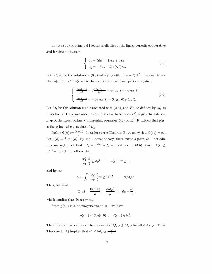
Let ρ(µ) be the principal Floquet multiplier of the linear periodic cooperative

and irreducible system

u′1 = (dµ2 − 1)u1 + αu2

u′2 = −βu2 + ∂zg(t, 0)u1.(3.5)

Let v(t, w) be the solution of (3.5) satisfying v(0, w) = w ∈ R2. It is easy to see

that u(t, x) = e−µxv(t, w) is the solution of the linear periodic system

∂u1(x,t)∂t = d∂2u1(x,t)

∂x2 − u1(x, t) + αu2(x, t)

∂u2(x,t)∂t = −βu2(x, t) + ∂zg(t, 0)u1(x, t).

(3.6)

Let Mt be the solution map associated with (3.6), and Btµ be defined by Mt as

in section 2. By above observation, it is easy to see that Btµ is just the solution

map of the linear ordinary differential equation (3.5) on R2. It follows that ρ(µ)

is the principal eigenvalue of Bωµ .

Define Φ(µ) := ln ρ(µ)µ . In order to use Theorem B, we show that Φ(∞) = ∞.

Let λ(µ) = 1ω ln ρ(µ). By the Floquet theory, there exists a positive ω-periodic

function w(t) such that v(t) = eλ(µ)tw(t) is a solution of (3.5). Since v′1(t) ≥(dµ2 − 1)v1(t), it follows that

w′1(t)

w1(t)≥ dµ2 − 1 − λ(µ), ∀t ≥ 0,

and hence

0 =

∫ ω

0

w′1(t)

w1(t)dt ≥ (dµ2 − 1 − λ(µ))ω.

Thus, we have

Φ(µ) =ln ρ(µ)

µ=ωλ(µ)

µ≥ ωdµ− ω

µ,

which implies that Φ(∞) = ∞.

Since g(t, ·) is subhomogeneous on R+, we have

g(t, z) ≤ ∂zg(t, 0)z, ∀(t, z) ∈ R2+.

Then the comparison principle implies that Qωφ ≤Mωφ for all φ ∈ Cu∗ . Thus,

Theorem B (1) implies that c∗ ≤ infµ>0lnρ(µ)

µ .

19

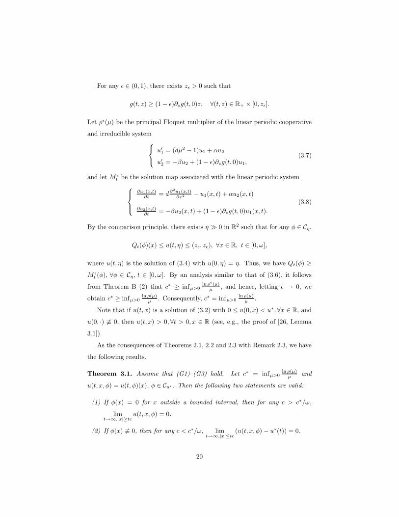
For any ε ∈ (0, 1), there exists zε > 0 such that

g(t, z) ≥ (1 − ε)∂zg(t, 0)z, ∀(t, z) ∈ R+ × [0, zε].

Let ρε(µ) be the principal Floquet multiplier of the linear periodic cooperative

and irreducible system

u′1 = (dµ2 − 1)u1 + αu2

u′2 = −βu2 + (1 − ε)∂zg(t, 0)u1,(3.7)

and let M εt be the solution map associated with the linear periodic system

∂u1(x,t)∂t = d∂2u1(x,t)

∂x2 − u1(x, t) + αu2(x, t)

∂u2(x,t)∂t = −βu2(x, t) + (1 − ε)∂zg(t, 0)u1(x, t).

(3.8)

By the comparison principle, there exists η 0 in R2 such that for any φ ∈ Cη,

Qt(φ)(x) ≤ u(t, η) ≤ (zε, zε), ∀x ∈ R, t ∈ [0, ω],

where u(t, η) is the solution of (3.4) with u(0, η) = η. Thus, we have Qt(φ) ≥M ε

t (φ), ∀φ ∈ Cη, t ∈ [0, ω]. By an analysis similar to that of (3.6), it follows

from Theorem B (2) that c∗ ≥ infµ>0lnρε(µ)

µ , and hence, letting ε → 0, we

obtain c∗ ≥ infµ>0ln ρ(µ)

µ . Consequently, c∗ = infµ>0lnρ(µ)

µ .

Note that if u(t, x) is a solution of (3.2) with 0 ≤ u(0, x) < u∗, ∀x ∈ R, and

u(0, ·) 6≡ 0, then u(t, x) > 0, ∀t > 0, x ∈ R (see, e.g., the proof of [26, Lemma

3.1]).

As the consequences of Theorems 2.1, 2.2 and 2.3 with Remark 2.3, we have

the following results.

Theorem 3.1. Assume that (G1)–(G3) hold. Let c∗ = infµ>0ln ρ(µ)

µ and

u(t, x, φ) = u(t, φ)(x), φ ∈ Cu∗ . Then the following two statements are valid:

(1) If φ(x) = 0 for x outside a bounded interval, then for any c > c∗/ω,

limt→∞,|x|≥tc

u(t, x, φ) = 0.

(2) If φ(x) 6≡ 0, then for any c < c∗/ω, limt→∞,|x|≤tc

(u(t, x, φ) − u∗(t)) = 0.

20

Theorem 3.2. Assume that (G1)–(G3) hold, and let c∗ be defined as in The-

orem 3.1. Then for any c ≥ c∗/ω, (3.2) has a periodic traveling wave solution

U(t, x−tc) such that U(t, s) is nonincreasing in s ∈ R, and lims→−∞

U(t, s) = u∗(t)

and lims→∞

U(t, s) = 0. Moreover, for any c < c∗/ω, (3.2) has no traveling wave

U(t, x− tc) connecting u∗(t) to 0.

We note that the autonomous version of system (3.2) was studied earlier in

[29] for traveling waves and in [23] for spreading speeds and traveling waves.

4 A periodic delayed and diffusive equation

Let τ > 0 be fixed and C := C([−τ, 0],R). For any u ∈ C([−τ, σ) × R,R) with

σ > 0, and any (t, x) ∈ [0, σ)× ∈ R, we use ut(·, x) to denote the member of Cdefined by

ut(θ, x) = u(t+ θ, x), ∀θ ∈ [−τ, 0].

Consider a periodic delay differential equation with diffusion on R:

∂u(t, x)

∂t= d

∂2u(t, x)

∂x2+ f(t, u(t, x), u(t− τ, x)), t > 0, x ∈ R, (4.1)

where d > 0, f ∈ C1(R3+,R), and f(t, u, v) is ω-periodic in t for some ω > 0. We

need the following assumption on f to study the spreading speed and periodic

traveling waves for (4.1).

(F) f(·, 0, 0) ≡ 0, ∂f(t,u,v)∂v > 0, ∀(t, u, v) ∈ R3

+, and there is a real number

L > 0 such that f(t, L, L) ≤ 0 and for each t ≥ 0, f(t, ·, ·) is strictly

subhomogeneous on [0, L]2 in the sense that f(t, αu, αv) > αf(t, u, v)

whenever α ∈ (0, 1), 0 < u, v ≤ L.

Define f : R+ × C → R by

f(t, φ) = f(t, φ(0), φ(−τ)), ∀(t, φ) ∈ R+ × C.

Then it is easy to see that for each t ≥ 0, f(t, ·) is quasimonotone on C in the

sense that f(t, φ) ≤ f(t, ψ) whenever φ ≤ ψ in C and φ(0) = ψ(0).

21

Let C be defined as in section 2 with H = R and k = 1, that is, C is the

space of all bounded and continuous functions from [−τ, 0] × R to R with the

compact open topology. Using the semigroup generated by the heat equation

and [15, Corollary 5] (see, e.g., the proof of [22, Theorem 2.2]), we can show

that (4.1) generates a monotone periodic semiflow Qt : CL → CL defined by

Qt(φ)(θ, x) = ut(θ, x, φ), ∀(θ, x) ∈ [−τ, 0] × R, φ ∈ CL,

where u(t, x, φ) is the unique solution of (4.1) satisfying u0(·, ·, φ) = φ ∈ CL.

Let Qt be the restriction of Qt to CL. It is easy to see that Qt : CL → CL

is the periodic semiflow generated by the following periodic delay differential

equationdu(t)

dt= f(t, u(t), u(t− τ)), t ≥ 0, (4.2)

with initial date u0 = φ ∈ CL. By the nonautonomous version of [21, Theorem

5.3.4], it follows that the map Qt is strongly monotone for t ≥ 2τ . Let r0 be the

spectral radius of the Poincare map associated with the linear periodic delay

differential equation

du(t)

dt= f ′

u(t, 0, 0)u(t) + f ′v(t, 0, 0)u(t− τ), t ≥ 0. (4.3)

Assume that r0 > 1. Then [27, Theorem 2.1] implies that system (4.2) has

a positive ω-periodic solution β(t), which is globally asymptotically stable in

CL \ 0. By the Dancer-Hess connecting orbit lemma (see, e.g., [9, Proposition

2.1]), the map Qω admits a strongly monotone full orbit connecting 0 to β :=

β(0). Thus, assumption (A5) holds for the map Qω.

Define the linear operator L(t) : C → C, t ≥ 0, by the relation

L(t)φ(θ, x) =

φ(t+ θ, x) − φ(0, x), t+ θ < 0, x ∈ R

0, t+ θ ≥ 0, −τ ≤ θ ≤ 0, x ∈ R.

Clearly, L(t) = 0 for t ≥ τ . Define S(t) := Qt − L(t), t ≥ 0. By the smoothing

property of the semigroup associated with the heat equation, it then follows

that Qt satisfies (A6)(a) for t ≥ τ , and (A6)(b) with ς = t for t ∈ (0, τ) (see also

22

the proof of [8, Theorem 6.1]). Now it is easy to see that the map Qω satisfies

all assumptions (A1)–(A6).

Let r(µ) be the spectral radius of the Poincare map associated with the

following linear periodic delay differential equation

dv(t)

dt= dµ2v(t) + f ′

u(t, 0, 0)v(t) + f ′v(t, 0, 0)v(t− τ). (4.4)

Then [27, Theorem 2.1] implies that r(µ) > 0. Furthermore, we have the fol-

lowing result on the spreading speed c∗ of the Poincare map Qω associated with

(4.1).

Lemma 4.1. Let c∗ be the asymptotic speed of spread of the map Qω. Then

c∗ = infµ>0ln r(µ)

µ .

Proof. Since f(t, ·) is subhomogeneous on [0, L]2, it follows from [28, Lemma

2.3.2] that

f(t, u, v) ≤ f ′(t, 0, 0)u+ f ′v(t, 0, 0)v, ∀(u, v) ∈ [0, L]2.

We fix a positive number α such that α + f ′u(t, 0, 0) > 0, ∀t ∈ [0, ω]. Let

f(t, u, v) := αu+ f(t, u, v). Then f ′u(t, 0, 0) > 0, f ′

v(t, 0, 0) > 0, ∀t ∈ [0, ω]. It is

easy to see that for any ε ∈ (0, 1), there exists δ = δ(ε) ∈ (0, L) such that

f(t, u, v) ≥ (1 − ε)f ′u(t, 0, 0)u+ (1 − ε)f ′

v(t, 0, 0)v, ∀(u, v) ∈ [0, δ]2.

Since f(t, u, v) = −αu+ f(t, u, v), we further have

f(t, u, v) ≥ [(1 − ε)f ′(t, 0, 0) − εα]u+ (1 − ε)f ′v(t, 0, 0)v, ∀(u, v) ∈ [0, δ]2.

Let v(t, φ) be the solution of the linear periodic equation (4.4) satisfying

v0 = φ ∈ C. It is easy to see that u(t, x) = e−µxv(t, φ) is the solution of the

linear periodic delay differential equation with diffusion

∂u

∂t= d

∂2u(t, x)

∂x2+ f ′

u(t, 0, 0)u(t, x) + f ′v(t, 0, 0)u(t− τ, x). (4.5)

Let Mt be the solution map associated with (4.5), and Btµ be defined by Mt as

in section 2. By above observation, it is easy to see that Btµ is just the solution

map of the linear functional differential equation (4.4) on C.

23

By the proof of [27, Theorem 2.1], it follows that there exists a positive ω-

periodic function w(t) such that v(t) = eλ(µ)tw(t) is a solution of (4.4), where

λ(µ) = 1ω ln r(µ). Define ψ ∈ C by ψ(θ) = eλ(µ)θw(θ), ∀θ ∈ [−τ, 0]. Clearly,

v(t, ψ) = eλ(µ)tw(t), ∀t ≥ 0. Then we have

Btµ(ψ)(θ) = v(t+ θ, ψ) = eλ(µ)teλ(µ)θ)w(t+ θ), ∀θ ∈ [−τ, 0], t ≥ 0.

By the ω-periodicity of w(t), it follows that

Bωµ (ψ)(θ) = eλ(µ)ωeλ(µ)θw(θ) = eλ(µ)ωψ(θ), ∀θ ∈ [−τ, 0],

that is, Bωµ (ψ) = eλ(µ)ωψ. This implies that eλ(µ)ω is the principal eigenvalue

of Bωµ with positive eigenfunction ψ. Then we have

Φ(µ) :=1

µln(

eλ(µ)ω)

=λ(µ)ω

µ=

ln r(µ)

µ.

By a similar argument as in section 3, we can show that Φ(∞) = ∞. Thus,

Theorem B (1) implies that c∗ ≤ infµ>0ln r(µ)

µ .

For any ε ∈ (0, 1), let rε(µ) be the spectral radius of the Poincare map

associated with the linear periodic delay differential equation

dv(t)

dt= dµ2v(t) + [(1 − ε)f ′(t, 0, 0)− εα]v(t) + (1 − ε)f ′

v(t, 0, 0)v(t− τ).

By an analysis similar to that of (4.4), it follows from Theorem B (2) that

c∗ ≥ infµ>0ln rε(µ)

µ , and hence, letting ε → 0, we have c∗ ≥ infµ>0ln r(µ)

µ .

Consequently, c∗ = infµ>0ln r(µ)

µ .

By Theorems 2.1, 2.2 and 2.3, we then have the following result.

Theorem 4.1. Assume that (F) holds and r0 > 1. Let c∗ be defined as in

Lemma 4.1. Then the following statements are valid:

(1) For any c > c∗/ω, if φ ∈ Cβ with 0 ≤ φ β, and φ(·, x) = 0 for x outside

a bounded interval, then limt→∞,|x|≥tc

u(t, x, φ) = 0.

(2) For any c < c∗, if φ ∈ Cβ with φ 6≡ 0, then limt→∞,|x|≤tc

(u(t, x, φ)−β(t)) = 0.

24

Theorem 4.2. Assume that (F) holds and r0 > 1. Let c∗ be defined as in

Lemma 4.1. Then for any c ≥ c∗/ω, (4.1) has a periodic traveling wave solution

U(t, x−ct) connecting β(t) to 0 such that U(t, s) is continuous and nonincreasing

in s ∈ R. Moreover, for any c < c∗/ω, (4.1) has no traveling wave U(t, x− ct)

connecting β(t) to 0.

5 A reaction-diffusion equation in a cylinder

We consider the ω-periodic reaction-diffusion equation in a cylinder

∂u∂t = ∂2u

∂x2 + ∆yu+ ug(t, y, u), x ∈ R, y = (y1 · · · , ym) ∈ Ω, t > 0,

∂u∂ν = 0 onR × ∂Ω × (0,+∞),

(5.1)

where Ω is a bounded domain in Rm with smooth boundary ∂Ω, ∆y =m∑

i=1

∂2

∂y2i

,

and ν is the outer unit normal vector to ∂Ω × R. Assume that

(G) g ∈ C1(R+×Ω×R+,R), ω-periodic in t, ∂g∂u < 0, ∀(t, y, u) ∈ R+×Ω×R+,

and there is K > 0 such that g(t, y,K) ≤ 0, ∀(t, y) ∈ R+ × Ω.

Let µ0 be the principal eigenvalue of the periodic-parabolic eigenvalue prob-

lem

∂v∂t = ∆yv + vg(t, y, 0) + µv, y ∈ Ω,

∂v∂ν = 0 on ∂Ω,

v ω − periodic in t

(5.2)

with a positive eigenfunction ϕ(t, y), ω-periodic in t (see [9, Section II.14]).

Assume that µ0 < 0. By [28, Theorem 3.1.5], it then follows that the reaction-

diffusion equation

∂u∂t = ∆yu+ ug(t, y, u), y ∈ Ω, t > 0,

∂v∂ν = 0 on ∂Ω × (0,+∞),

(5.3)

admits a unique positive periodic solution β(t, y), which is globally asymptot-

ically stable in C(Ω,R+) \ 0. Moreover, the Dancer-Hess connecting orbit

lemma (see, e.g., [9, Proposition 2.1]) implies that the Poincare map associated

with (5.3) admits a strongly monotone full orbit connecting 0 to β := β(0, ·).

25

Let C be the set of all bounded and continuous functions from R × Ω to R.

We consider the linear equation

∂u∂t = ∂2u

∂x2 + ∆yu, x ∈ R, y ∈ Ω, t > 0,

∂v∂ν = 0 on R × ∂Ω × (0,+∞).

(5.4)

Let G(t, y, w) be the Green function of the equation (see, e.g., [7])

∂u∂t = ∆yu, y ∈ Ω, t > 0,

∂v∂ν = 0 on ∂Ω × (0,+∞).

(5.5)

Then it is easy to verify that e−(x−z)2

4πt G(t, y, w) is the Green function of equation

(5.4), that is, the solution of (5.4) with initial value u(0, ·) = φ(·) ∈ C can be

expressed as

u(t, x, y, φ) = 1√4πt

∫ +∞−∞

∫

Ωe−

(x−z)2

4πt G(t, y, w)φ(z, w)dwdz.

Define T (t)φ = u(t, ·, φ), ∀φ ∈ C. It then follows that T (t)∞t=0 is a linear

semigroup on the space C with respect to the compact open topology. For any

a, b ∈ C, define [a, b]C := φ ∈ C, a ≤ φ ≤ b. For any t > 0 and a, b ∈ C, it is

easy to verify that T (t)[a, b]C is a family of equicontinuous functions.

Now we write (5.1) subject to u(0, ·) = φ ∈ C as an integral equation

u(t, x, y) = T (t)[φ](x, y) +∫ t

0 T (s)f(t− s, y, u(t− s, x, y))ds, (5.6)

where f(t, y, u) = ug(t, y, u). Using the standard linear semigroup theory (see,

e.g., [17, 15]), we see that for any φ ∈ CK , (5.1) has a unique solution u(t, φ)

with u(0, φ) = φ, which exists globally on [0,+∞). Define Qt(φ) = u(t, φ).

With the expression of the semigroup T (t) and (5.6), we can show that Qt∞t=0

is a subhomogeneous ω-periodic semiflow on CK . Moreover, for each t > 0,

Qt satisfies hypotheses (A1),(A2), (A3)(a), (A4), (A5) and (A6)(a) with [−τ, 0]

replaced by Ω.

Let Mt∞t=0 be the periodic semiflow associated with the linear equation

∂u∂t = ∂2u

∂x2 + ∆yu+ ug(t, y, 0), x ∈ R, y ∈ Ω, t > 0,

∂u∂ν = 0 on R × ∂Ω × (0,+∞).

(5.7)

26

Since g(t, y, 0) ≥ g(t, y, u), we have Mt[φ] ≥ Qt[φ] for any φ ∈ Cβ. Let M εt be

the periodic semiflow associated with the linear equation

∂u∂t = ∂2u

∂x2 + ∆yu+ (1 − ε)ug(t, y, 0), x ∈ R, y ∈ Ω, t > 0,

∂u∂ν = 0 on R × ∂Ω × (0,+∞).

(5.8)

Then for any ε, there is a δ 0 such that M εt [φ] ≤ Qt[φ] for any φ ∈ Cδ and

t ∈ [0, ω].

Let ρ ∈ R be a parameter. It is easy to see that if η(t, y) is a solution of the

linear equation

∂u∂t = ∆yu+ ug(y, 0) + ρ2u, y ∈ Ω, t > 0,

∂u∂ν = 0 on ∂Ω × (0,+∞),

(5.9)

then u(t, x, y) = η(t, y)e−ρx is a solution of (5.7). Define

Btρ[α](y) = Mt[α(y)e−ρx](0, y), ∀α ∈ C := C(Ω,R), y ∈ Ω.

It follows that Btµ is the solution map associated with (5.9). Let µρ := µ0 − ρ2.

It is easy to verify that e−µρtϕ(t, y) is a solution of (5.9). Thus, we have

Btρ[ϕ(0, ·)] = e−µρtϕ(t, ·), ∀t ≥ 0,

and hence

Bωρ [ϕ(0, ·)] = e−µρωϕ(ω, ·) = e−µρωϕ(0, ·).

This implies that e−µρω is the principal eigenvalue of Bωρ with positive eigen-

function ϕ(0, ·). Define

Φ(ρ) :=ln e−µρω

ρ=

(

ρ− µ0

ρ

)

ω.

Clearly, Φ(∞) = ∞. Let c∗ be the spreading speed of Qω. Note that that Mω

satisfies (C1)-(C7). By similar arguments as in sections 3 and 4, it follows from

Theorem B that c∗ = infρ>0

Φ(ρ) == 2ω√−µ0.

Note that if u(t, x, y) is a solution of (5.1) with 0 ≤ u(0, x, y) < β(y), ∀y ∈Ω, x ∈ R, and u(0, x, y) 6≡ 0, then u(t, x, y) > 0, ∀t > 0, y ∈ Ω, x ∈ R (see, e.g.,

the proof of [26, Lemma 3.1]).

As the consequences of Theorems 2.1, 2.2 and 2.3 with Remark 2.4, we have

the following results.

27

Theorem 5.1. Assume that (G) holds and µ0 < 0. Let u(t, x, y) be a solution

of (5.1) with u(0, ·) ∈ Cβ. Then the following two statements are valid:

(1) If u(0, x, y) = 0 for y ∈ Ω and x outside a bounded interval, then for any

c > 2√−µ0, lim

t→∞,|x|≥tcu(t, x, y) = 0 uniformly for y ∈ Ω.

(2) If u(0, x, y) 6≡ 0, then for any c < 2√−µ0, lim

t→∞,|x|≤tc(u(t, x, y) − β(t, y)) =

0 uniformly for y ∈ Ω.

Theorem 5.2. Assume that (G) holds and µ0 < 0. For any c ≥ 2√−µ0,

(5.1) has a periodic traveling wave solution U(t, x− tc, y) such that U(t, s, y) is

nonincreasing in s ∈ R, and lims→−∞

U(t, s, y) = β(t, y) and lims→∞

U(t, s, y) = 0

uniformly for y ∈ Ω. Moreover, for any c < 2√−µ0, (5.1) has no traveling wave

U(t, x− tc, y) connecting β(t, ·) to 0.

We should mention that some autonomous parabolic equations in cylinders

were studied earlier in [4, 13] for traveling waves and in [11] for spreading speeds

and traveling waves.

Acknowledgment: X.-Q. Zhao would like to thank Georgia Institute of

Technology for its kind hospitality during his leave there.

References

[1] N. D. Alikakos, P. W. Bates and X. Chen, Periodic traveling waves and

locating oscillating patterns in multidimensional domains, Trans. Amer.

Math. Soc., 351(1999), 2777–2805.

[2] D. G. Aronson and H. F. Weinberger, Nonlinear diffusion in population

genetics, combustion, and nerve pulse propagation, Partial Differential

Equations and Related Topics, J. A. Goldstein, ed., 5–49, Lecture Notes in

Mathematics Ser., 446, Springer-Verlag, 1975.

[3] P. Bates and F. Chen, Periodic traveling waves for a nonlocal integro-

differential model, Electric J. Differential Equations, 26(1999), 1–19.

28

[4] H. Berestycki and L. Nirenberg, Traveling fronts in cylinders, Ann. Inst.

H. Poincare Anal. NonLinaire, 9(1992), 497–572.

[5] V. Capasso, Mathematical Structures of Epidemic Systems, Lecture Notes

in Biomath. 97, Springer-Verlag, Heidelberg, 1993.

[6] F. Chen, Almost periodic traveling waves of nonlocal evolution equations,

Nonlinear Analysis, 50(2002), 807–838.

[7] M. G. Garroni and J. L. Menaldi, Green Functions for Second Order

Parabolic Integro-differential Problems, Longman Scientific & Technical,

Harlow, 1992.

[8] J. K. Hale and S. M. Verduyn Lunel, Introduction to Functional Differen-

tial Equations, Springer-Verlag, New York, 1993.

[9] P. Hess, Periodic-Parabolic Boundary Value Problems and Positivity, Long-

man Scientific and Technical, New York, 1991.

[10] B. Li, H. F. Weinberger and M. A. Lewis, Spreading speeds as slowest wave

speeds for cooperative systems, Math. Biosci., in press.

[11] X. Liang and X.-Q. Zhao, Asymptotic speeds of spread and traveling waves

for monotone semiflows with applications, Communications on Pure and

Appl. Math., in press.

[12] R. Lui, Biological growth and spread modeled by systems of recursions, I.

Mathematical theory, Math. Biosci., 93(1989), 269–295.

[13] J.-F. Mallordy and J.-M. Roquejoffre, A parabolic equation of the KPP

type in higher dimensions, SIAM J. Math. Anal., 26(1995), 1–20.

[14] R. H. Martin, Nonlinear Operators and Differential Equations in Banach

Spaces, John Wiley & Sons, 1976.

[15] R. H. Martin and H. L. Smith, Abstract functional differential equations

and reaction-diffusion systems, Trans. Amer. Math. Soc., 321(1990), 1–44.

29

[16] R. D. Nussbaum, Eigenvectors of nonlinear positive operator and the linear

Krein-Rutman theorem, in Fixed Point Theory, Lecture Notes in Mathe-

matics, Vol. 886, pp.309-331, Springer-Verlag, New York/Berlin, 1981.

[17] A. Pazy, Semigroups of Linear Operators and Applications to Partial Dif-

ferential Equations, Springer-Verlag, New York, 1983.

[18] W. Shen, Traveling waves in time almost periodic structures governed by

bistable nonlinearities, I & II, J. Differential Equations, 159(1999), 1–101.

[19] W. Shen, Dynamical systems and traveling waves in almost periodic struc-

tures, J. Differential Equations, 169(2001), 493–548.

[20] W. Shen, Traveling waves in time periodic lattice differential equations,

Nonlinear Analysis, 54(2003), 319–339.

[21] H. L. Smith, Monotone Dynamical Systems: An introduction to the theory

of competitive and cooperative systems, Math Surveys and Monographs 41,

American Mathematical Society, Providence, RI, 1995.

[22] H. L. Smith and X.-Q. Zhao, Global asymptotic stability of traveling waves

in delayed reaction-diffusion equations, SIAM J. Math. Anal., 31(2000),

514–534.

[23] H. R. Thieme and X.-Q. Zhao, Asymptotic speeds of spread and travel-

ing waves for integral equations and delayed reaction-diffusion models, J.

Differential Equations, 195(2003), 430–470.

[24] H. F. Weinberger, Long-time behavior of a class of biological models, SIAM

J. Math. Anal., 13(1982), 353–396.

[25] H. F. Weinberger, M. A. Lewis and B. Li, Analysis of linear determinacy

for spread in cooperative models, J. Math. Biol., 45(2002), 183–218.

[26] D. Xu and X.-Q. Zhao, Bistable waves in an epidemic model, J. Dynamics

and Differential Equations, 16(2004), 679–707.

30

[27] D. Xu and X.-Q. Zhao, Dynamics in a periodic competitive model with

stage structure, J. Math. Anal. Appl., 311(2005), 417–438.

[28] X.-Q. Zhao, Dynamical Systems in Population Biology, Springer-Verlag,

New York, 2003.

[29] X.-Q. Zhao and W. Wang, Fisher waves in an epidemic model, Discrete

and Continuous Dynamical Systems (Ser. B), 4(2004), 1117–1128.

31