Spectroscopy of High-Redshift Supernovae from the ESSENCE Project: The First 2 Years

arX

iv:a

stro

-ph/

0411

357v

1 1

2 N

ov 2

004

Spectroscopy of High-Redshift Supernovae from the ESSENCE Project: The

First Two Years1

Thomas Matheson,2 Stephane Blondin,3 Ryan J. Foley,4 Ryan Chornock,4 Alexei V. Filippenko,4

Bruno Leibundgut,3 R. Chris Smith, 5 Jesper Sollerman,6 Jason Spyromilio,3 Robert P.

Kirshner,7 Alejandro Clocchiatti,8 Claudio Aguilera,5 Brian Barris,9 Andrew C. Becker,10 Peter

Challis,7 Ricardo Covarrubias,10 Peter Garnavich,11 Malcolm Hicken,7,12 Saurabh Jha,4 Kevin

Krisciunas,11 Weidong Li,4 Anthony Miceli,10 Gajus Miknaitis,13 Jose Luis Prieto,14 Armin Rest,5

Adam G. Riess,15 Maria Elena Salvo,16 Brian P. Schmidt,16 Christopher W. Stubbs,7,12 Nicholas

B. Suntzeff,5 and John L. Tonry9

http://arXiv.org/abs/astro-ph/0411357v1

– 2 –

ABSTRACT

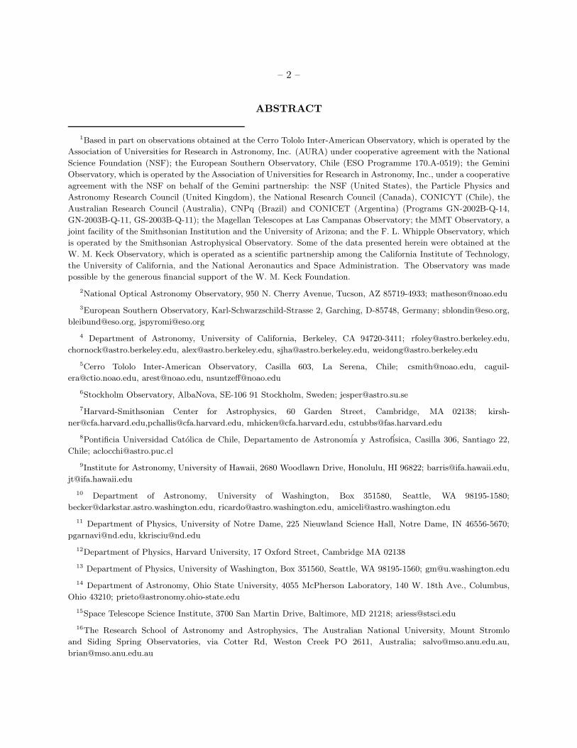
1Based in part on observations obtained at the Cerro Tololo Inter-American Observatory, which is operated by the

Association of Universities for Research in Astronomy, Inc. (AURA) under cooperative agreement with the National

Science Foundation (NSF); the European Southern Observatory, Chile (ESO Programme 170.A-0519); the Gemini

Observatory, which is operated by the Association of Universities for Research in Astronomy, Inc., under a cooperative

agreement with the NSF on behalf of the Gemini partnership: the NSF (United States), the Particle Physics and

Astronomy Research Council (United Kingdom), the National Research Council (Canada), CONICYT (Chile), the

Australian Research Council (Australia), CNPq (Brazil) and CONICET (Argentina) (Programs GN-2002B-Q-14,

GN-2003B-Q-11, GS-2003B-Q-11); the Magellan Telescopes at Las Campanas Observatory; the MMT Observatory, a

joint facility of the Smithsonian Institution and the University of Arizona; and the F. L. Whipple Observatory, which

is operated by the Smithsonian Astrophysical Observatory. Some of the data presented herein were obtained at the

W. M. Keck Observatory, which is operated as a scientific partnership among the California Institute of Technology,

the University of California, and the National Aeronautics and Space Administration. The Observatory was made

possible by the generous financial support of the W. M. Keck Foundation.

2National Optical Astronomy Observatory, 950 N. Cherry Avenue, Tucson, AZ 85719-4933; [email protected]

3European Southern Observatory, Karl-Schwarzschild-Strasse 2, Garching, D-85748, Germany; [email protected],

[email protected], [email protected]

4 Department of Astronomy, University of California, Berkeley, CA 94720-3411; [email protected],

[email protected], [email protected], [email protected], [email protected]

5Cerro Tololo Inter-American Observatory, Casilla 603, La Serena, Chile; [email protected], caguil-

[email protected], [email protected], [email protected]

6Stockholm Observatory, AlbaNova, SE-106 91 Stockholm, Sweden; [email protected]

7Harvard-Smithsonian Center for Astrophysics, 60 Garden Street, Cambridge, MA 02138; kirsh-

[email protected],[email protected], [email protected], [email protected]

8Pontificia Universidad Catolica de Chile, Departamento de Astronomia y Astrofisica, Casilla 306, Santiago 22,

Chile; [email protected]

9Institute for Astronomy, University of Hawaii, 2680 Woodlawn Drive, Honolulu, HI 96822; [email protected],

[email protected]

10 Department of Astronomy, University of Washington, Box 351580, Seattle, WA 98195-1580;

[email protected], [email protected], [email protected]

11 Department of Physics, University of Notre Dame, 225 Nieuwland Science Hall, Notre Dame, IN 46556-5670;

[email protected], [email protected]

12Department of Physics, Harvard University, 17 Oxford Street, Cambridge MA 02138

13 Department of Physics, University of Washington, Box 351560, Seattle, WA 98195-1560; [email protected]

14 Department of Astronomy, Ohio State University, 4055 McPherson Laboratory, 140 W. 18th Ave., Columbus,

Ohio 43210; [email protected]

15Space Telescope Science Institute, 3700 San Martin Drive, Baltimore, MD 21218; [email protected]

16The Research School of Astronomy and Astrophysics, The Australian National University, Mount Stromlo

and Siding Spring Observatories, via Cotter Rd, Weston Creek PO 2611, Australia; [email protected],

[email protected]

– 3 –

We present the results of spectroscopic observations of targets discovered during the

first two years of the ESSENCE project. The goal of ESSENCE is to use a sample

of ∼200 Type Ia supernovae (SNe Ia) at moderate redshifts (0.2 . z . 0.8) to place

constraints on the equation of state of the Universe. Spectroscopy not only provides

the redshifts of the objects, but also confirms that some of the discoveries are indeed

SNe Ia. This confirmation is critical to the project, as techniques developed to determine

luminosity distances to SNe Ia depend upon the knowledge that the objects at high

redshift are the same as the ones at low redshift. We describe the methods of target

selection and prioritization, the telescopes and detectors, and the software used to

identify objects. The redshifts deduced from spectral matching of high-redshift SNe Ia

with low-redshift SNe Ia are consistent with those determined from host-galaxy spectra.

We show that the high-redshift SNe Ia match well with low-redshift templates. We

include all spectra obtained by the ESSENCE project, including 52 SNe Ia, 5 core-

collapse SNe, 12 active galactic nuclei, 19 galaxies, 4 possibly variable stars, and 16

objects with uncertain identifications.

Subject headings: galaxies: distances and redshifts — cosmology: distance scale —

supernovae: general

1. Introduction

The revolution wrought in modern cosmology using luminosity distances of Type Ia supernovae

(SNe Ia) (Schmidt et al. 1998; Riess et al. 1998; Perlmutter et al. 1999; Riess et al. 2001; Knop et al.

2003; Tonry et al. 2003; Barris et al. 2004; Riess et al. 2004b) relies upon the fact that the objects

so employed are, in fact, SNe of Type Ia. Although the light-curve shape alone is useful (e.g.,

Barris & Tonry 2004), the only way to be sure of the true nature of an object as a SN Ia is through

spectroscopy. The calculation of luminosity distances depends upon the high-redshift objects being

SNe Ia so that low-redshift calibration methods can be employed. The classification scheme for

SNe is based upon the optical spectrum near maximum (see Filippenko 1997, for a review of SN

types), so rest-wavelength optical spectroscopy is necessary to properly identify SNe Ia at high

redshifts. Despite this significance, relatively little attention has been paid to the spectroscopy of

the high-redshift SNe Ia, with some notable exceptions (Coil et al. 2000). Other publications that

include high-redshift SN Ia spectra include Schmidt et al. (1998), Riess et al. (1998), Perlmutter et

al. (1998), Leibundgut & Sollerman (2001), Tonry et al. (2003), Barris et al. (2004), Blondin et al.

(2004), Riess et al. (2004b), and Lidman et al. (2004).

In addition to providing evidence for the acceleration of the expansion of the Universe, it was

recognized at an early stage that high-redshift SNe Ia could put constraints on the equation of

state for the Universe (Garnavich et al. 1998), parameterized as w = P/(ρc2), the ratio of the dark

energy’s pressure to its density. To further explore this, the ESSENCE project was begun. The

– 4 –

ESSENCE (Equation of State: SupErNovae trace Cosmic Expansion) project is a five-year ground-

based SN survey designed to place constraints on the equation-of-state parameter for the Universe

using ∼200 SNe Ia over a redshift range of 0.2 . z . 0.8 (see Miknaitis et al. 2005; Smith et al.

2005, for a more extensive discussion of the goals and implementation of the ESSENCE project).

Spectroscopic identification of optical transients is a major component of the ESSENCE

project. In addition to confirming some targets as SNe Ia, the spectroscopy provides redshifts,

allowing the derived luminosity distances to be compared with a given cosmological model. So

many targets are discovered during the ESSENCE survey that a large amount of telescope time

on 6.5 m to 10 m telescopes is required. In the first two years of the program, we were fortunate

enough to have been awarded over 60 nights at large-aperture telescopes. Even with this much

time, though, our resources were insufficient to spectroscopically identify all of the potentially use-

ful candidates. This remains the most significant limiting factor in achieving the ESSENCE goal

of finding, identifying, and following the desired number of SNe Ia with the appropriate redshift

distribution.

Nonetheless, spectroscopic observations of ESSENCE targets in the time available have been

successful, with almost fifty SNe Ia clearly identified, and several more characterized as likely SNe Ia.

Other identifications include core-collapse SNe, active galactic nuclei (AGNs), and galaxies. The

galaxy spectra may include an unidentified SN component.

This paper will describe the results of the spectroscopic component of the first two years of

the ESSENCE program. Year One refers to our 2002 Sep-Dec campaign; Year Two was our 2003

Sep-Dec campaign. In Section 2, we describe the process of target selection and prioritization.

Section 3 describes the technical aspects of the observations. We discuss target identification in

Section 4. The summary of results in terms of types of objects and success rates is given in Section

5. In addition, we present in Section 5 all of the spectra obtained, including those of the SNe Ia

(with low-redshift templates), core-collapse SNe, AGNs, galaxies, stars, and objects that remain

unidentified.

2. Target Selection

The ESSENCE survey uses the Blanco 4 m telescope at CTIO with the MOSAIC wide-field

CCD camera to detect many kinds of optical transients (Smith et al. 2005). Temporal coverage helps

to identify solar-system objects such as Kuiper Belt Objects (KBOs) and asteroids. Known AGNs

and variable stars can also be eliminated from the possible SN Ia list. The remaining transients

are all potentially SNe. They are also faint, requiring large-aperture telescopes to obtain spectra

of the quality necessary to securely identify the object. Exposure times on 8-10 m telescopes are

typically about half an hour, but can be as much as two hours. Such telescope time is difficult

to obtain in quantity, so not all of the detected transients can be examined spectroscopically. We

apply several criteria to prioritize target selection for spectroscopic observation.

– 5 –

The first step in sorting targets is based upon the spectroscopic resources available. The

equatorial fields used for the ESSENCE program are accessible from most major astronomical

sites, so the main concern with matching targets to spectroscopic telescopes is the aperture size of

the telescope. The ESSENCE targets are generally in the range 18 . mR . 24 mag. When 8-10 m

telescopes are unavailable, the fainter targets become lower in priority. The limit for low-dispersion

spectroscopy to identify SNe with the 6.5 m telescopes is mR ≈ 22 − 23 mag, although this will

vary with weather conditions and seeing. If the full range of telescopes is available, then targets

are prioritized by magnitude for observation at a given telescope. The longitudinal distribution of

spectroscopic resources can be important if confirmation of a high-priority target is made during

a night when multiple spectroscopic resources are available. By the time a target is confirmed,

the fields may have set for telescopes in Chile, while they are still accessible from Hawaii. This

requires active, real-time collaboration between the group finding SN candidates and those running

the spectroscopic observations.

One advantage of the ESSENCE program is that fields are imaged in multiple filters, allowing

for discrimination of targets by color. Tonry et al. (2003) present a table of expected SN Ia peak

magnitudes as a function of redshift; see also Poznanski et al. (2002), Gal-Yam et al. (2004), Riess

et al. (2004a), Strolger et al. (2004), and Smith et al. (2005) for discussions of color selection for

SN candidates. Given apparent R-band and I-band magnitudes, one can calculate the R − I color

and compare that with an expected color for those magnitudes. The cadence of the ESSENCE

program (returning to the same field every four days) will likely catch SNe at early phases (i.e.,

before maximum brightness). Early core-collapse SNe are bluer than SNe Ia, as are AGNs. For

example, when selecting for higher-redshift targets, objects with R − I . 0.2 mag were considered

unlikely to be SNe Ia, while objects with R−I & 0.4 mag were made high priority for spectroscopic

observation. The exact values of R − I used for selection depended on the observed R-band

magnitude. This method was used more consistently in the last month of Year Two, reducing the

fraction of spectroscopic targets that were identified as AGNs from ∼ 10% over the lifetime of the

project to ∼ 5% during that month.

The cadence of the ESSENCE program is designed to catch SNe early. At the start of an

observing campaign or after periods of bad weather, though, we may have missed SNe during their

rise to maximum brightness and only caught them while they are declining from maximum. If a

target is brightening, then it is a higher priority than one that is not. This prioritization by phase of

the SN became even more important when our Hubble Space Telescope (HST ) program to observe

some of the ESSENCE SNe Ia was active (see Krisciunas et al. 2005). The response time of HST

for a new target, even if the rough position on the sky is known from our chosen search fields, is

still on the order of several days. To ensure that HST was not generally looking at SNe Ia after

maximum brightness, we would emphasize targets for spectroscopic identification that appeared to

be at an early epoch. In addition, we chose fainter objects, as higher-redshift SNe Ia were a prime

motivation for HST photometry. The HST observations, while still targets of opportunity, were

scheduled for specific ESSENCE search fields, so new targets in those fields were given the highest

– 6 –

priority.

The position of the SN in the host galaxy also influences the priority for observation. An

optical transient located at the core of a galaxy is often an AGN, rather than an SN. The color

selection described above is a less-biased predictor. In addition, even if the object is an SN, the

signal of the SN itself is diluted by the light of the galaxy, making proper identification difficult.

Objects that are well-separated from the host galaxy are given a higher priority. Being too far from

the galaxy can, however, present another problem—the difficulty in obtaining a spectrum of the

host in addition to the SN. Without a high signal-to-noise ratio (S/N) spectrum of the host, there

is no precise measure of the redshift. This is especially true if the host galaxy cannot be included

in the slit with the target, either to orient the slit at the parallactic angle or as a result of other

observational constraints. In addition, host galaxies can be faint, so the large luminosity contrast

with the SN makes detection of the host problematic (the so-called “hostless” SNe), although we

did not reject any candidates solely for this reason. The best compromise is to have an object

well separated from the host, but with the host still in the spectrograph slit. Without narrow-

line features from the host (either emission or absorption lines), the redshift can be difficult to

determine. This lack of a host-galaxy spectrum became less of a concern, though, as we found that

the SN spectrum itself is a relatively accurate, if less precise, measure of the redshift (see discussion

below). The light curve alone can be used to estimate distances in a redshift-independent way

(Barris & Tonry 2004), but only with a well-sampled and accurate light curve.

The target selection process is complex and dynamic. Biases are introduced by some of the

steps; for example, SN candidates near the centers of galaxies are less likely to be observed. Since

the goal is to optimize the spectroscopic telescope time to identify SNe Ia in a specific redshift

range, we have chosen these selection processes as our best compromise. The biases introduced

may make the sample of SNe Ia identified problematic for uses in statistical studies of the nature

of SNe Ia at high redshift.

3. Observations

Spectroscopic observations of ESSENCE targets were obtained at a wide variety of telescopes:

the Keck I and II 10 m telescopes, the VLT 8 m telescopes, the Gemini North and South 8 m

telescopes, the Magellan Baade and Clay 6.5 m telescopes, the MMT 6.5 m telescope, and the

Tillinghast 1.5 m telescope at the F. L. Whipple Observatory (FLWO). The spectrographs used

were LRIS (Oke et al. 1995) with Keck I, ESI (Sheinis et al. 2002) with Keck II, FORS1 with VLT

(Appenzeller et al. 1998), GMOS (Hook et al. 2002) at Gemini (North and South), IMACS (Dressler

2004) with Baade, LDSS2 (Mulchaey 2001) with Clay, the Blue Channel (Schmidt et al. 1989) at

MMT, and FAST (Fabricant et al. 1998) at FLWO. Nod-and-shuffle techniques (Glazebrook &

Bland-Hawthorn 2001) were used with GMOS (North and South) and IMACS to improve sky

subtraction in the red portion of the spectrum.

– 7 –

Standard CCD processing and spectrum extraction were accomplished with IRAF17. Most

of the data were extracted using the optimal algorithm of Horne (1986); for the VLT data, an

alternative extraction method based upon Richardson-Lucy restoration (Blondin et al. 2004) was

employed. Low-order polynomial fits to calibration-lamp spectra were used to establish the wave-

length scale. Small adjustments derived from night-sky lines in the object frames were applied. We

employed IRAF and our own IDL routines to flux calibrate the data and, in most cases, to remove

telluric lines using the well-exposed continua of the spectrophotometric standards (Wade & Horne

1988; Matheson et al. 2000).

4. Target Identification

Once a calibrated spectrum is available, the next step is to properly classify the object. For

brighter objects that yield high S/N spectra, an SN is often easy to distinguish and classify. Most of

the ESSENCE targets are faint enough to be difficult objects even for large-aperture telescopes. The

resulting noisy spectra can be confusing. Even for well-exposed spectra, though, exact classification

can occasionally still be challenging.

For SNe, the classification scheme is based upon the optical spectrum near maximum brightness

(Filippenko 1997). Type II SNe are distinguished by the presence of hydrogen lines. The Type

I SNe lack hydrogen, and are further subdivided by the presence or absence of other features. The

hallmark of SNe Ia is a strong Si II λ6355 absorption feature. Near maximum brightness, this

absorption is blueshifted by ∼10,000 km s−1 and appears near 6150 A. In SNe Ib, this line is not as

strong, and the optical helium series dominates the spectrum. The SNe Ic lack all these identifying

lines.

At high redshift, the Si II λ6355 feature is at wavelengths inaccessible to optical spectrographs,

so the identification relies upon the pattern of features in the rest-frame ultraviolet (UV) and blue-

optical wavelengths. The Ca II H&K λλ3934, 3968 doublet is a distinctive feature in SNe Ia, but it

is also present in SNe Ib/c, so the overall pattern is important for a clear identification as a SN Ia.

Other important features to identify SNe Ia include Si II λ4130, Mg II λ4481, Fe II λ4555, Si III

λ4560, S II λ4816, and Si II λ5051 (see, e.g., Coil et al. 2000; Jeffery et al. 1992; Kirshner et al.

1993; Mazzali et al. 1993).

The first stage of classification is done by eye. Drawing upon the extensive experience of

the spectroscopic observers associated with ESSENCE, we can provide a solid evaluation of the

spectrum. Objects such as AGNs and normal galaxies are fairly easy to distinguish. The SNe Ia

are also often clear, but some fraction of the data will require more extensive analysis. The first

step is simply to make certain that the collective expertise is used, rather than just the individual

17IRAF is distributed by the National Optical Astronomy Observatory, which is operated by the Association of

Universities for Research in Astronomy, Inc., under cooperative agreement with the National Science Foundation.

– 8 –

at the telescope. Spectroscopic results are widely disseminated via e-mail and through an internal

web page, allowing rapid examination of any questionable spectrum by the entire collaboration.

Broad discussion often leads to a consensus.

In addition to the traditional by-eye approach, we employ automated comparisons. If the object

is likely to be a SN Ia, and if the S/N ratio is sufficiently high and the rest-wavelength coverage

appropriate, we can use a spectral-feature aging routine (Riess et al. 1997) that compares specific

components of the SN Ia spectrum with a library of SN Ia spectra at known phases. This can pin

down the epoch of a SN Ia to within a few days. This program, though, is limited to normal SNe Ia

(i.e., not spectroscopically peculiar objects, which are often overluminous or underluminous). In

addition, it does not identify objects that do not match the Type Ia SN spectra in the library.

For a more general identification routine, we use an algorithm called SuperNova IDentification

(SNID; Tonry et al. 2005). This program takes the input spectrum and compares it against a

library of objects of many types. The templates include SNe Ia of various luminosity classes and

at a range of ages, core-collapse SNe, and galaxies. The offset in wavelength caused by redshift

is a free parameter, so the output includes an estimate of the redshift of the object. The routine

compares the input with the library and returns the most likely match. The comparison is weighted

by the amount of overlap between the input spectrum and the template. For a subset of the objects

(. 10%), the SNID comparison is not optimal. This may be the result of contamination by galaxy

light, the lack of a matching template in the SNID library, poor S/N of the spectrum in question,

or a problem in the routine. All SNID comparisons are checked by eye for a qualitative judgment

of the goodness of fit.

The redshift of the object can also be directly determined from the spectrum itself if narrow

emission or absorption lines associated with the host galaxy are present. Occasionally, observations

are set up to include the host galaxy in the spectrograph slit specifically for the purpose of obtaining

a redshift. If there is a strong enough signal of a galaxy spectrum, but no clearly identifiable narrow

emission or absorption lines, cross-correlation with an absorption template could be used. For the

spectra that had narrow emission or absorption lines (or were cross-correlated with a template),

we report the redshift to three significant digits. If the redshift determination is based solely on a

comparison of the SN spectrum to a low-redshift analog, the redshift is less certain, and we only

report the value to two significant digits.

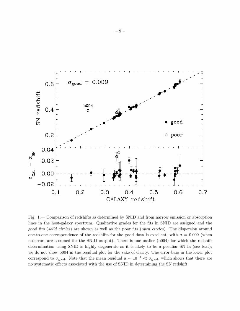
For the objects with a more precise redshift derived from the host galaxy, we can compare

the galactic redshift with the value of the redshift estimated by SNID. Figure 1 shows that the

SNID redshifts agree well with the galaxy redshifts. Thus, for objects without precise redshifts

from host galaxy spectra, the SNID redshifts can be used as reliable substitutes. In the cases where

SNID did not agree with a galaxy redshift, we forced the redshift to match in order to find the

best-fitting template, but all the supernova-based redshifts reported in this paper correspond to

the “un-forced” SNID result.

– 9 –

Fig. 1.— Comparison of redshifts as determined by SNID and from narrow emission or absorption

lines in the host-galaxy spectrum. Qualitative grades for the fits in SNID are assigned and the

good fits (solid circles) are shown as well as the poor fits (open circles). The dispersion around

one-to-one correspondence of the redshifts for the good data is excellent, with σ = 0.009 (when

no errors are assumed for the SNID output). There is one outlier (b004) for which the redshift

determination using SNID is highly degenerate as it is likely to be a peculiar SN Ia (see text);

we do not show b004 in the residual plot for the sake of clarity. The error bars in the lower plot

correspond to σgood. Note that the mean residual is ∼ 10−4 ≪ σgood, which shows that there are

no systematic effects associated with the use of SNID in determining the SN redshift.

– 10 –

5. Results

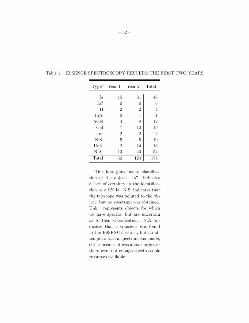
The results of our spectroscopic observations during the first two years of the ESSENCE

program are summarized in Table 1. There are 46 SNe Ia (and 5 additional likely SNe Ia), along

with 5 core-collapse SNe. Note also that there were 54 transients in the first two years that were not

observed spectroscopically. Through the target selection methods described in Section 2, we were

able to prioritize the more likely candidates, but many of these were not observed solely because of

the lack of sufficient spectroscopic resources. This became more of an issue toward the end of Year

Two, when good weather and increasingly efficient detection algorithms increased the number of

transients discovered.

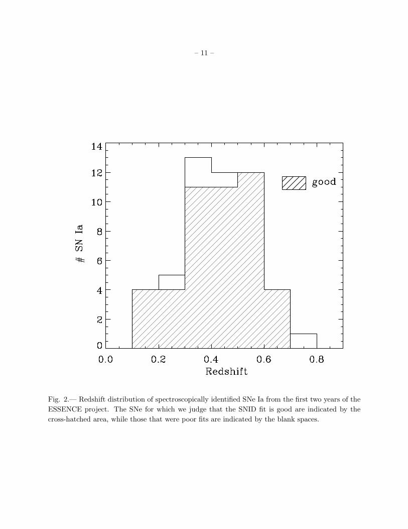
The goal of the ESSENCE project is to find ∼200 SNe Ia over the redshift range 0.2 . z .

0.8. In Figure 2, we show the actual distribution in redshift of the SNe Ia from the ESSENCE

project that are spectroscopically confirmed. There are SNe over the entire targeted redshift range,

although there are fewer at the high end (z & 0.6). A significant fraction of the signal of w is

accessible at z ≈ 0.5 (Miknaitis et al. 2005), but a goal for the last three years of the program is

to ensure that the SNe Ia observed spectroscopically are distributed optimally over our targeted

redshift range. This highlights the importance of the 8-10 m telescopes such as Gemini, the VLT,

and Keck that are critical to spectroscopy of the faint objects at the high-redshift end of our range.

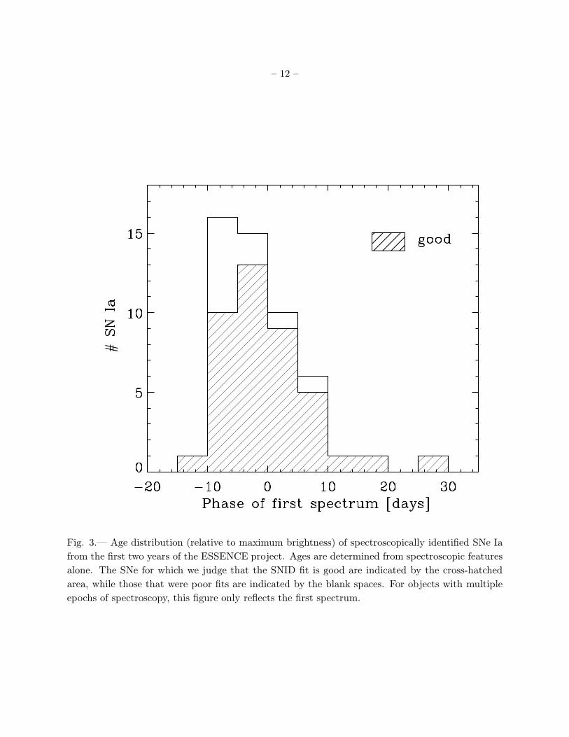
Both SNID and the spectral-feature aging method described in Section 4 give an indication

of the age of the SN Ia. Light curves will provide a more precise measure of the age of the SN

at the time of the spectroscopy, but an estimate of the epoch of the spectrum to within a few

days is possible from the spectral features alone. Figure 3 shows the distribution in age (relative

to maximum brightness) at the time of spectroscopy (not discovery, as spectra are often taken

up to several days after discovery). In the 15 cases18 where we have spectra of the same SN Ia

at multiple epochs, the relative ages are consistent with the times of the spectroscopic exposures

(also considering the effects of cosmological time dilation and probable errors of the fits of ∼ ±3

days). There is one exception to this consistency (b027), but at later epochs when the spectra are

changing less.

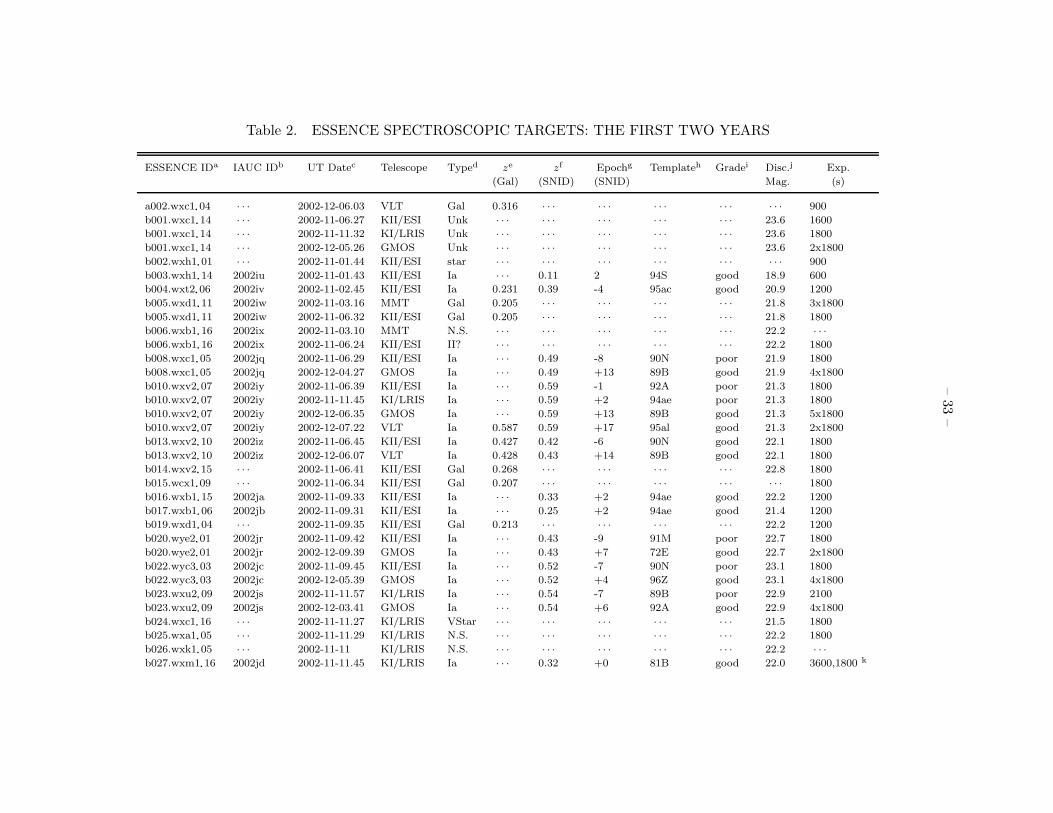
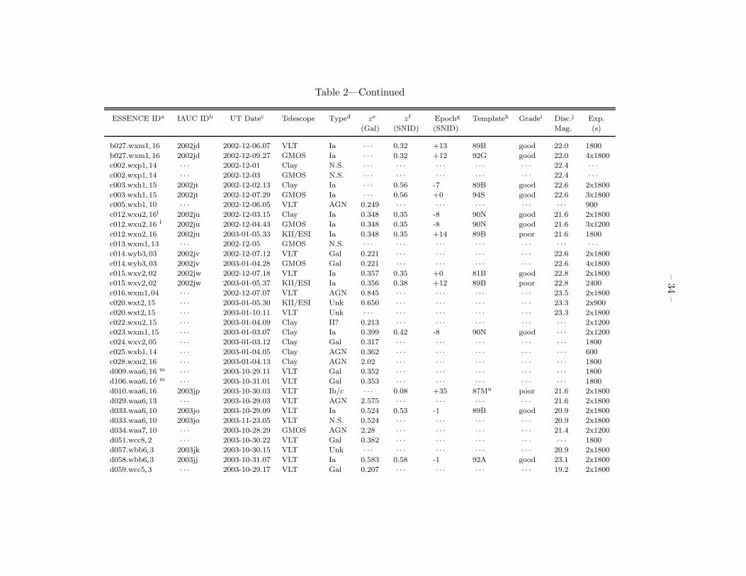
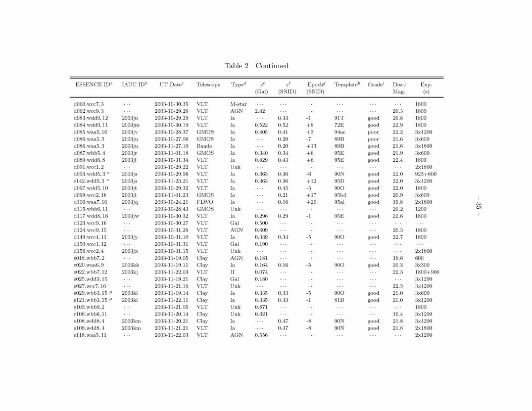
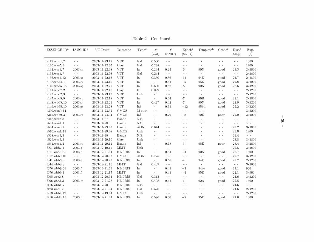
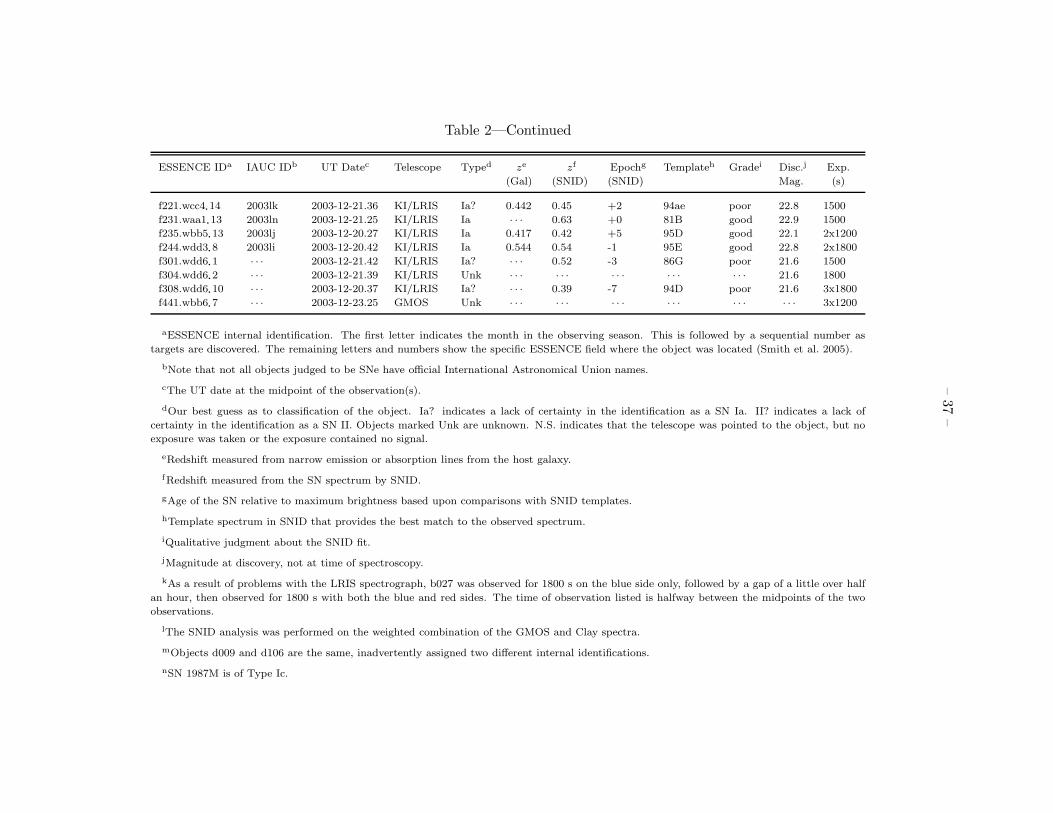
Table 2 is a list of all ESSENCE targets that were selected for spectroscopic identification.

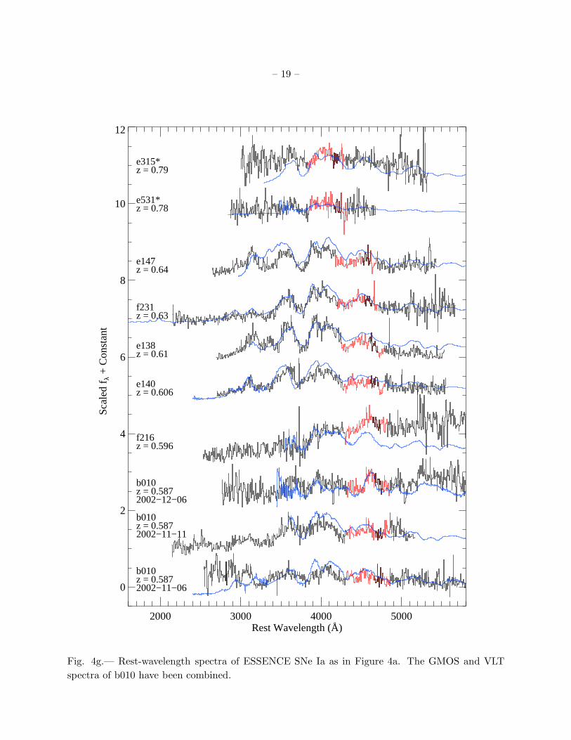
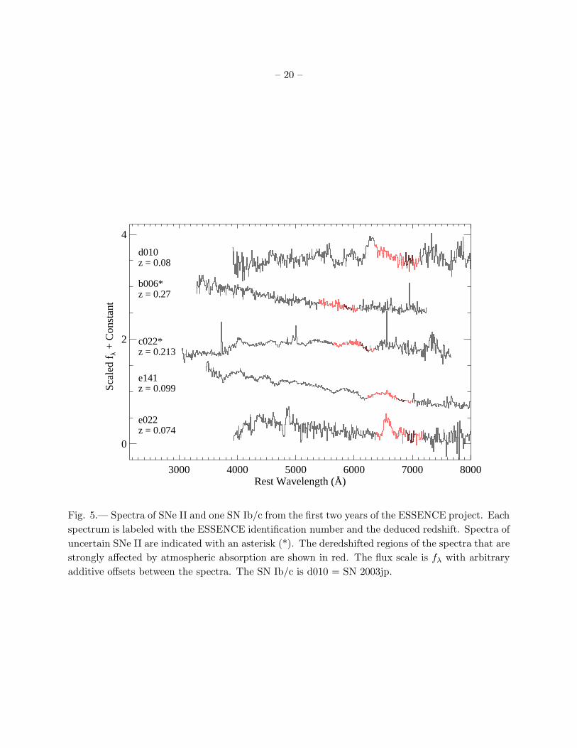
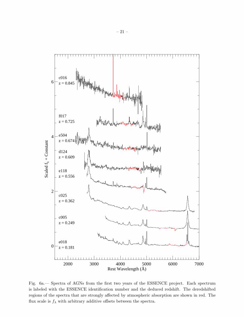
The results for these first two years include 52 SNe Ia or likely SNe Ia (Figure 4), 4 SNe II (Figure

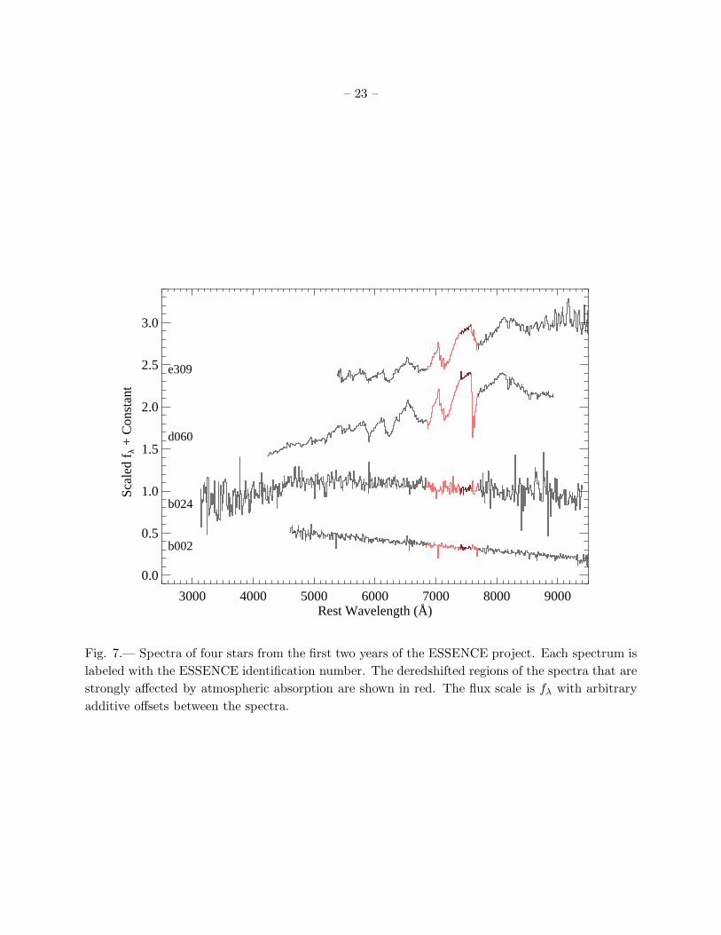
5), 1 SN Ib/c (Figure 5), 12 AGNs (Figure 6), 4 possibly variable stellar objects (Figure 7), 19

galaxies (Figure 8), and 16 objects of unknown classification (Figure 9). There were 10 objects for

which we pointed the telescope at the target and did not get a spectrum, either because of poor

sky conditions or the target was actually a solar-system object and had moved out of the field.

No attempt has been made to remove host-galaxy contamination for any object presented in

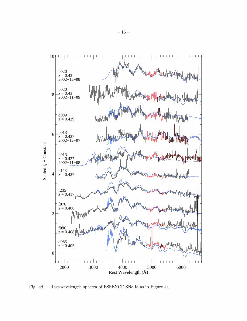
Figures 4 and 5. The amount of galaxy light is significant for some objects (e.g., f221 on Figure 4d).

18These are b008, b010, b013, b020, b022, b023, b027, c003, c012, c015, d086, d093, e029, e108, and f076.

– 11 –

Fig. 2.— Redshift distribution of spectroscopically identified SNe Ia from the first two years of the

ESSENCE project. The SNe for which we judge that the SNID fit is good are indicated by the

cross-hatched area, while those that were poor fits are indicated by the blank spaces.

– 12 –

Fig. 3.— Age distribution (relative to maximum brightness) of spectroscopically identified SNe Ia

from the first two years of the ESSENCE project. Ages are determined from spectroscopic features

alone. The SNe for which we judge that the SNID fit is good are indicated by the cross-hatched

area, while those that were poor fits are indicated by the blank spaces. For objects with multiple

epochs of spectroscopy, this figure only reflects the first spectrum.

– 13 –

3000 4000 5000 6000 7000 8000Rest Wavelength (Å)

0

2

4

6

8

10

Sca

led

f λ +

Con

stan

t

z = 0.11b003

z = 0.16d100

z = 0.164e020

2003−10−27z = 0.20d086

2003−11−27z = 0.20d086

z = 0.21d099

z = 0.231b004

z = 0.244e132

z = 0.25b017

z = 0.296d117

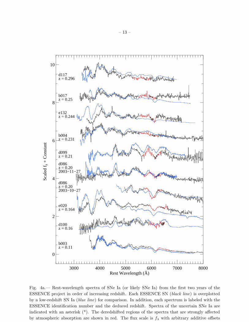
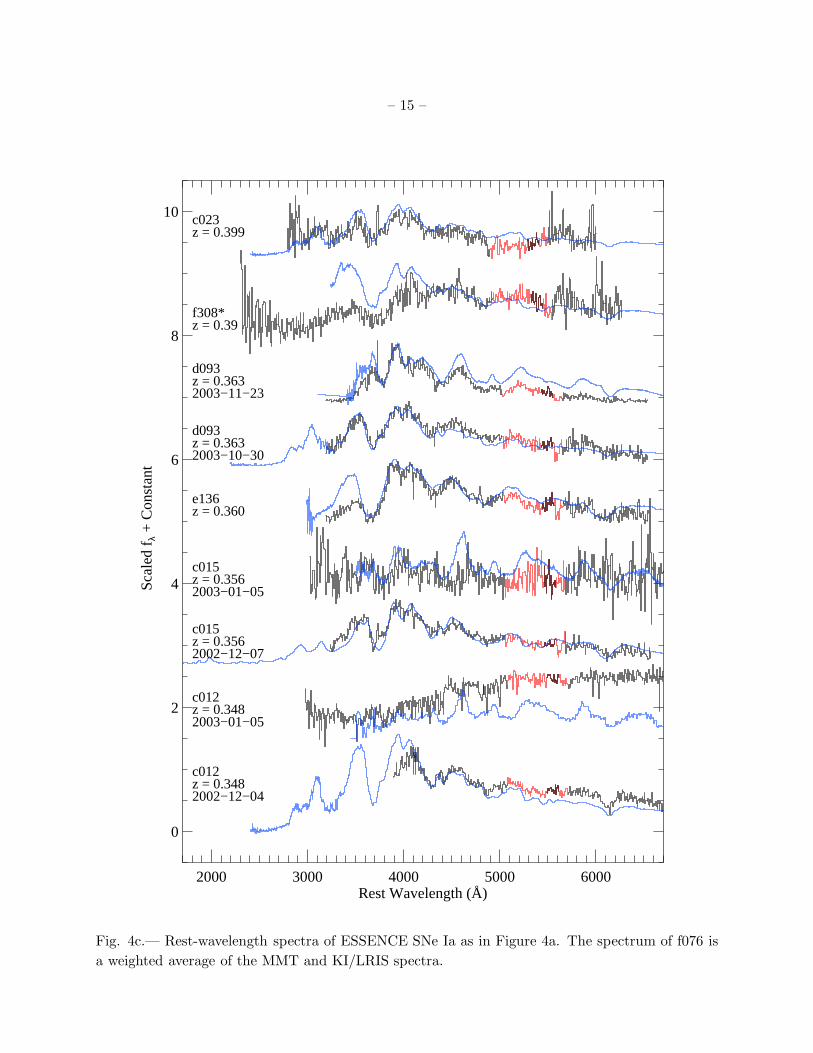
Fig. 4a.— Rest-wavelength spectra of SNe Ia (or likely SNe Ia) from the first two years of the

ESSENCE project in order of increasing redshift. Each ESSENCE SN (black line) is overplotted

by a low-redshift SN Ia (blue line) for comparison. In addition, each spectrum is labeled with the

ESSENCE identification number and the deduced redshift. Spectra of the uncertain SNe Ia are

indicated with an asterisk (*). The deredshifted regions of the spectra that are strongly affected

by atmospheric absorption are shown in red. The flux scale is fλ with arbitrary additive offsets

between the spectra.

– 14 –

3000 4000 5000 6000 7000Rest Wavelength (Å)

0

2

4

6

8

Sca

led

f λ +

Con

stan

t

2002−11−11z = 0.32b027

2002−12−06z = 0.32b027

2002−12−07z = 0.32b027

z = 0.33b016

z = 0.33d083

2003−11−19z = 0.335e029

2003−11−22z = 0.335e029

z = 0.339d149

z = 0.340d087

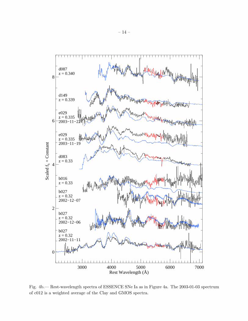
Fig. 4b.— Rest-wavelength spectra of ESSENCE SNe Ia as in Figure 4a. The 2003-01-03 spectrum

of c012 is a weighted average of the Clay and GMOS spectra.

– 15 –


0

2

4

6

8

10

Sca

led

f λ +

Con

stan

t

2002−12−04z = 0.348c012

2003−01−05z = 0.348c012

2002−12−07z = 0.356c015

2003−01−05z = 0.356c015

z = 0.360e136

2003−10−30z = 0.363d093

2003−11−23z = 0.363d093

z = 0.39f308*

z = 0.399c023

Fig. 4c.— Rest-wavelength spectra of ESSENCE SNe Ia as in Figure 4a. The spectrum of f076 is

a weighted average of the MMT and KI/LRIS spectra.

– 16 –


0

2

4

6

8

10

Sca

led

f λ +

Con

stan

t

z = 0.405d085

z = 0.408f096

z = 0.406f076

z = 0.417f235

z = 0.427e148

2002−11−08z = 0.427b013

2002−12−07z = 0.427b013

z = 0.429d089

2002−11−09z = 0.43b020

2002−12−09z = 0.43b020

Fig. 4d.— Rest-wavelength spectra of ESSENCE SNe Ia as in Figure 4a.

– 17 –


0

2

4

6

8

10

Sca

led

f λ +

Con

stan

t

z = 0.442f221*

z = 0.45d097

2003−11−20z = 0.47e108

2003−11−21z = 0.47e108

2002−11−06z = 0.49b008

2002−11−0z = 0.49b008

z = 0.51e149*

z = 0.52f301*

2002−11−09z = 0.52b022

2002−12−05z = 0.52b022

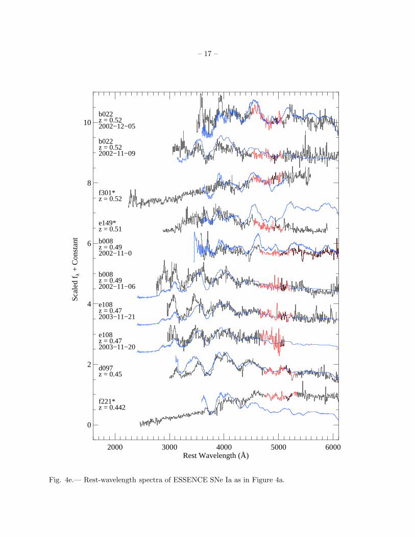
Fig. 4e.— Rest-wavelength spectra of ESSENCE SNe Ia as in Figure 4a.

– 18 –

2000 3000 4000 5000Rest Wavelength (Å)

0

2

4

6

8

10

Sca

led

f λ +

Con

stan

t

z = 0.522d084

z = 0.524d033

z = 0.54f011

2002−11−11z = 0.54b023

2002−12−03z = 0.54b023

z = 0.544f244

2002−12−02z = 0.56c003

2002−12−07z = 0.56c003

z = 0.56f041

z = 0.583d058

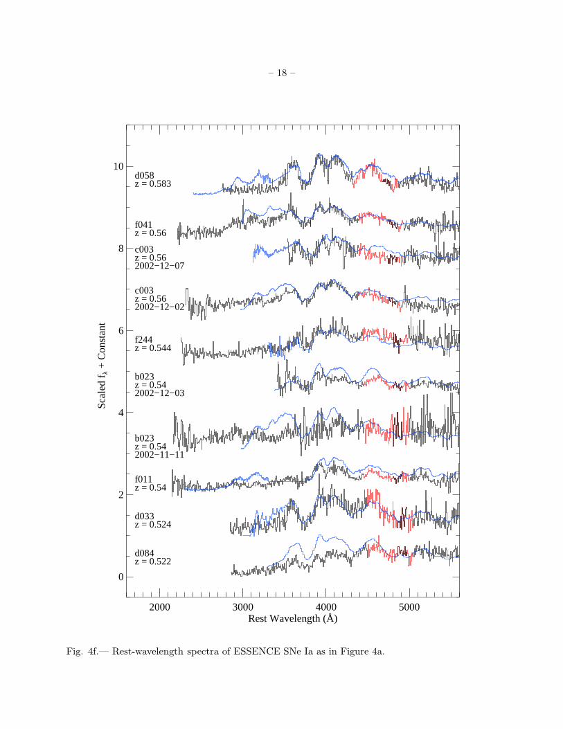
Fig. 4f.— Rest-wavelength spectra of ESSENCE SNe Ia as in Figure 4a.

– 19 –

2000 3000 4000 5000Rest Wavelength (Å)

0

2

4

6

8

10

12

Sca

led

f λ +

Con

stan

t

2002−11−06z = 0.587b010

2002−11−11z = 0.587b010

2002−12−06z = 0.587b010

z = 0.596f216

z = 0.606e140

z = 0.61e138

z = 0.63f231

z = 0.64e147

z = 0.78e531*

z = 0.79e315*

Fig. 4g.— Rest-wavelength spectra of ESSENCE SNe Ia as in Figure 4a. The GMOS and VLT

spectra of b010 have been combined.

– 20 –


0

2

4

Sca

led

f λ +

Con

stan

t

z = 0.074e022

z = 0.099e141

z = 0.213c022*

z = 0.27b006*

z = 0.08d010

Fig. 5.— Spectra of SNe II and one SN Ib/c from the first two years of the ESSENCE project. Each

spectrum is labeled with the ESSENCE identification number and the deduced redshift. Spectra of

uncertain SNe II are indicated with an asterisk (*). The deredshifted regions of the spectra that are

strongly affected by atmospheric absorption are shown in red. The flux scale is fλ with arbitrary

additive offsets between the spectra. The SN Ib/c is d010 = SN 2003jp.

– 21 –


0

2

4

6

Sca

led

f λ +

Con

stan

t

z = 0.181e018

z = 0.249c005

z = 0.362c025

z = 0.556e118

z = 0.609d124

z = 0.674e504

z = 0.725f017

z = 0.845c016

Fig. 6a.— Spectra of AGNs from the first two years of the ESSENCE project. Each spectrum

is labeled with the ESSENCE identification number and the deduced redshift. The deredshifted

regions of the spectra that are strongly affected by atmospheric absorption are shown in red. The

flux scale is fλ with arbitrary additive offsets between the spectra.

– 22 –


0

2

Sca

led

f λ +

Con

stan

t

z = 2.02c028

z = 2.28d034

z = 2.419d062

z = 2.575d029

Ly α

C IV

C III

Mg II

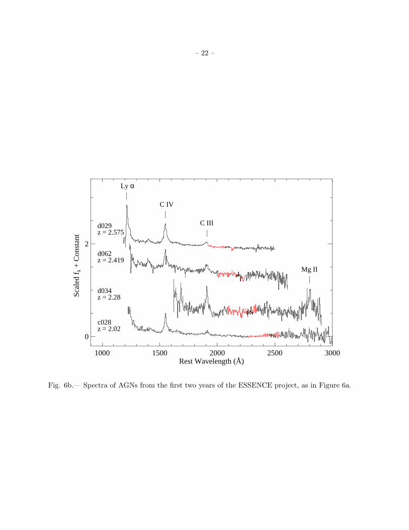
Fig. 6b.— Spectra of AGNs from the first two years of the ESSENCE project, as in Figure 6a.

– 23 –

3000 4000 5000 6000 7000 8000 9000Rest Wavelength (Å)

0.0

0.5

1.0

1.5

2.0

2.5

3.0

Sca

led

f λ +

Con

stan

t

b002

b024

d060

e309

Fig. 7.— Spectra of four stars from the first two years of the ESSENCE project. Each spectrum is

labeled with the ESSENCE identification number. The deredshifted regions of the spectra that are

strongly affected by atmospheric absorption are shown in red. The flux scale is fλ with arbitrary

additive offsets between the spectra.

– 24 –


0

2

4

6

8

Sca

led

f λ +

Con

stan

t

z = 0.180e025

z = 0.190d150

z = 0.205b005

z = 0.207d059

z = 0.207b015

z = 0.213b019

z = 0.221c014

z = 0.244e133

z = 0.268b014

z = 0.298e120

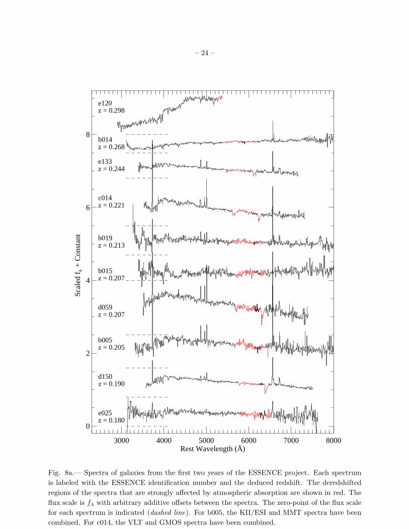
Fig. 8a.— Spectra of galaxies from the first two years of the ESSENCE project. Each spectrum

is labeled with the ESSENCE identification number and the deduced redshift. The deredshifted


flux scale is fλ with arbitrary additive offsets between the spectra. The zero-point of the flux scale

for each spectrum is indicated (dashed line). For b005, the KII/ESI and MMT spectra have been

combined. For c014, the VLT and GMOS spectra have been combined.

– 25 –


0

2

4

6

Sca

led

f λ +

Con

stan

t

z = 0.313f095

z = 0.316a002

z = 0.317c024

z = 0.352d009

z = 0.382d051

z = 0.409f044

z = 0.500d123

z = 0.526

f123

z = 0.560e119

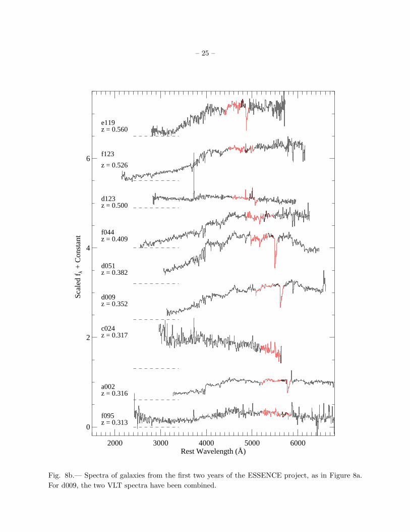
Fig. 8b.— Spectra of galaxies from the first two years of the ESSENCE project, as in Figure 8a.

For d009, the two VLT spectra have been combined.

– 26 –

3000 4000 5000 6000 7000 8000Observed Wavelength (Å)

0

2

4

6

8

Sca

led

f λ +

Con

stan

t

2002−11−06b001

2002−12−05b001

2003−01−05c020

2003−01−10c020

d057

d091

d115

d156

e027

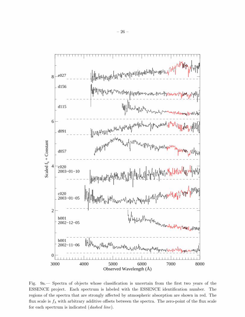
Fig. 9a.— Spectra of objects whose classification is uncertain from the first two years of the

ESSENCE project. Each spectrum is labeled with the ESSENCE identification number. The


flux scale is fλ with arbitrary additive offsets between the spectra. The zero-point of the flux scale

for each spectrum is indicated (dashed line).

– 27 –

3000 4000 5000 6000 7000 8000 9000Observed Wavelength (Å)

0

2

4

6

8

Sca

led

f λ +

Con

stan

t

z >= 0.871e103

Host z = 0.321e106

e143

e510

e529

f001

f213

f304

f441

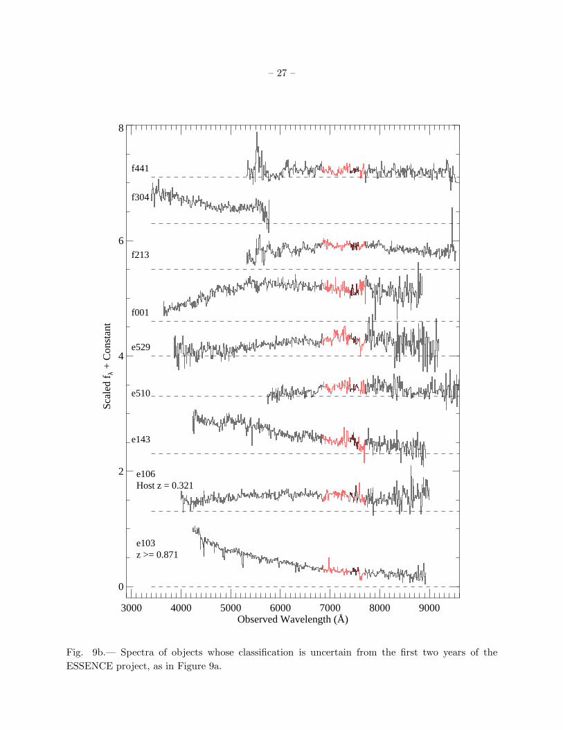
Fig. 9b.— Spectra of objects whose classification is uncertain from the first two years of the

ESSENCE project, as in Figure 9a.

– 28 –

In addition, no extinction corrections have been applied, either for Galactic reddening or extinction

in the host galaxy. Given the Galactic latitudes of the ESSENCE fields (Smith et al. 2005) and our

preference for targets well separated from the host galaxy, the effects of extinction are likely to be

minimal (Blondin et al. 2005; Foley et al. 2005).

For each SN Ia in Figure 4, the best match low-redshift comparison spectrum as determined

using SNID is included. In general, the high-redshift SNe Ia look very similar to those at low

redshift, implying that there are no significant evolutionary effects. Future papers will deal in

much greater detail with the comparison with low-redshift SNe Ia, as well as removal of galactic

contamination and the effects of extinction (Blondin et al. 2005; Foley et al. 2005).

While most of the high-redshift SNe Ia appear to be normal, there are some examples of

peculiar SNe Ia. Both b004 (SN 2002iv; Figure 4a) and d083 (SN 2003jn; Figure2b) show strong

similarities with SN 1991T, an overluminous Type Ia SN (Filippenko et al. 1992; Phillips et al.

1992). Given the high rate of peculiar SNe Ia at low redshift (Li et al. 2001), we would expect to

find such objects in a high-redshift sample.

We note that in Figure 4, there are several examples of high-redshift SNe Ia from the ESSENCE

sample for which the low-redshift template appears to be a poor match. Examples include d086

(2003-10-27), b008 (2002-11-06), e149, and b022 (2002-12-05) . The most likely explanation for this

is that the templates included in SNID do not cover the complete range of possibilities, although

problems with the spectrum (e.g., poor S/N or sky subtraction) may also play a role. Rather

than perform a non-objective search for the best match, we leave these as examples of the current

limitations in SNID. We plan to expand the SNID templates to eliminate such occurrences in the

future.

Two unusual cases in the sample of SNe Ia spectra are e315 (SN 2003ku) and b004 (SN 2002iv).

They are the only SNe for which the redshift determination in SNID was ambiguous. For e315, if

we assume that it is a Ia, then the best fit redshift is 0.79, but a fit at a redshift of 0.41 is only

marginally worse. All other SNe Ia spectra in the ESSENCE sample had redshifts determined by

SNID that were unambiguous. If we rely on the spectrum alone, the SNID result of z = 0.79 is

what we would choose, and so we report it in this paper. Analysis presented by Krisciunas et

al. (2005) shows that neither of the redshifts suggested by SNID gives a very satisfactory fit to

the photometry. In the case of b004, the SNID result is z = 0.39, while the fit when z = 0.231,

known from galaxy features, is almost as good. As b004 is similar to SN 1991T (see above), the

lack of good templates in SNID may be the source of this discrepancy. Correlation of b004 with

SN 1991T templates yields a redshift of z = 0.22, close to the value derived from the host galaxy.

This highlights some of the perils of identifying optical transients with low S/N spectra. Sometimes

the spectrum alone is not enough. A consideration of all the information (spectrum, light curve,

host galaxy, etc.) is necessary to draw the appropriate conclusion.

Among the unknown spectra (Figure 9a), there are three spectra that require some discussion.

For e106, the redshift is known because the host galaxy was also observed. The emission line

– 29 –

appearing at the observed wavelength of 9457 A in f213 is real. If this is Hα then z = 0.44; if it is

[O III] λ5007, then z = 0.89. There is an apparent doublet absorption line in e103 at an observed

wavelength of 5240 A. We interpret this as Mg II λ2800 at a redshift of 0.871, implying that this

object has a redshift at least that high. It is likely to be a high-redshift AGN, but we do not have

enough information to move it out of the unknown category.

6. Conclusions

We have presented optical spectroscopy of the targets selected for follow-up observations from

the first two years of the ESSENCE project. As the target selection process has improved, we

have increased our yield of SNe Ia that are needed for the primary purpose of the ESSENCE

project—measuring luminosity distances to ∼200 SNe Ia over the redshift range (0.2 . z . 0.8).

The SNe Ia show strong similarities with low-redshift SNe Ia, implying that there are no significant

evolutionary changes in the nature of Type Ia SNe and that our methods for identifying objects

have been successful. This is also shown by the concordance of redshifts derived from SN spectra

and those found from the host galaxy itself. Over the next three years, ESSENCE will continue to

discover high-redshift SNe Ia. With enough spectroscopic telescope time, we plan to be even more

successful in correctly identifying Type Ia SNe than we have been during the first two years.

All spectra presented in this paper will be made publicly available upon publication.

We would like to thank the staffs of the Paranal, Gemini, Keck, Las Campanas, MMT, F. L.

Whipple, and Cerro Tololo Inter-American Observatories for their extensive assistance and support

during this project. We would also like to thank Warren Brown and Craig Heinke for assistance

with the MMT observations. This work is supported primarily by NSF grants AST-0206329 and

AST-0443378. In addition, A.V.F.’s group at UC Berkeley acknowledges NSF grant AST-0307894.

C.W.S thanks the McDonnell Foundation and Harvard University for their support. A.C. acknowl-

edges the support of CONICYT (Chile) through FONDECYT grants 1000524 and 7000524.

REFERENCES

Appenzeller, I., et al. 1998, The Messenger, 94, 1

Barris, B. J., & Tonry, J. L. 2004, ApJ, 613, L21

Barris, B. J., et al. 2004, ApJ, 602, 571

Blondin, S., Walsh, J. R., Leibundgut, B., & Sainton, G. 2004, A&A, in press (astro-ph/0410406)

Blondin, S., et al. 2005, in preparation

– 30 –

Coil, A. L., et al. 2000, ApJ, 544, L111

Dressler, A. 2004,

http://www.ociw.edu/lco/magellan/instruments/IMACS/observing with IMACS 2.html

Fabricant, D., Cheimets, P., Caldwell, N., & Geary, J. 1998, PASP, 110, 79

Filippenko, A. V. 1997, ARA&A, 35, 309

Filippenko, A. V., et al. 1992, ApJ, 384, L15

Foley, R. J., et al. 2005, in preparation

Gal-Yam, A., Poznanski, D., Maoz, D., Filippenko, A. V., & Foley, R. J. 2004, PASP, 116, 597

Garnavich, P. M., et al. 1998, ApJ, 509, 74

Glazebrook, K., & Bland-Hawthorn, J. 2001, PASP, 113, 197

Hook, I., et al. 2002, SPIE, 4841

Horne, K. 1986, PASP, 98, 609

Jeffery, D. J., Leibundgut, B., Kirshner, R. P., Benetti, S., Branch, D., & Sonneborn, G. 1992,

ApJ, 397, 304

Kirshner, R. P., et al. 1993, ApJ, 415, 589

Knop, R. A., et al. 2003, ApJ, 598, 102

Krisciunas, K., et al. 2005, in preparation

Leibundgut, B., & Sollerman, J. 2001, Europhysics News, 32, 121

Li, W., Filippenko, A. V., Treffers, R. R., Riess, A. G., Hu, J., & Qiu, Y. 2001, ApJ, 546, 734

Lidman, C., et al. 2004, A&A, in press (astro-ph/0410506)

Matheson, T., Filippenko, A. V., Ho, L. C., Barth, A. J., & Leonard, D. C. 2000, AJ, 120, 1499

Mazzali, P. A., Lucy, L. B., Danziger, I. J., Gouiffes, C., Cappellaro, E., & Turatto, M. 1993, A&A,

269, 423

Miknaitis, G., et al. 2005, in preparation

Mulchaey, J. 2001, http://www.ociw.edu/lco/magellan/instruments/LDSS2/ldss2 usersguide.html

Oke, J. B., et al. 1995, PASP, 107, 375

Perlmutter, S., et al. 1998, Nature, 391, 51

– 31 –

Perlmutter, S., et al. 1999, ApJ, 517, 565

Phillips, M. M., Wells, L. A., Suntzeff, N. B., Hamuy, M., Leibundgut, B., Kirshner, R. P., & Foltz,

C. B. 1992, AJ, 103, 1632

Poznanski, D., Gal-Yam, A., Maoz, D., Filippenko, A. V., Leonard, D. C., & Matheson, T. 2002,

PASP, 114, 833

Riess, A. G., et al. 1997, AJ, 114, 722

Riess, A. G., et al. 1998, AJ, 116, 1009

Riess, A. G., et al. 2001, ApJ, 560, 49

Riess, A. G., et al. 2004a, ApJ, 600, L163

Riess, A. G., et al. 2004b, ApJ, 607, 665

Schmidt, B. P., et al. 1998, ApJ, 507, 46

Schmidt, G., Weymann, R., & Foltz, C. 1989, PASP, 101, 713

Sheinis, A. I., Bolte, M., Epps, H. W., Kibrick, R. I., Miller, J. S., Radovan, M. V., Bigelow, B. C.,

& Sutin, B. M. 2002, PASP, 114, 851

Smith, R. C., et al. 2005, in preparation

Strolger, L., et al. 2004, ApJ, 613, 200

Tonry, J. L., et al. 2003, ApJ, 594, 1

Tonry, J. L., et al. 2005, in preparation

Wade, R. A., & Horne, K. D. 1988, ApJ, 324, 411

This preprint was prepared with the AAS LATEX macros v5.2.

– 32 –

Table 1. ESSENCE SPECTROSCOPY RESULTS: THE FIRST TWO YEARS

Typea Year 1 Year 2 Total

Ia 15 31 46

Ia? 0 6 6

II 2 2 4

Ib/c 0 1 1

AGN 4 8 12

Gal 7 12 19

star 2 2 4

N.S. 5 5 10

Unk. 2 14 16

N.A. 13 43 54

Total 50 124 174

aOur best guess as to classifica-

tion of the object. Ia? indicates

a lack of certainty in the identifica-

tion as a SN Ia. N.S. indicates that

the telescope was pointed to the ob-

ject, but no spectrum was obtained.

Unk. represents objects for which

we have spectra, but are uncertain

as to their classification. N.A. in-

dicates that a transient was found

in the ESSENCE search, but no at-

tempt to take a spectrum was made,

either because it was a poor target or

there were not enough spectroscopic

resources available.

–33

–

Table 2. ESSENCE SPECTROSCOPIC TARGETS: THE FIRST TWO YEARS

ESSENCE IDa IAUC IDb UT Datec Telescope Typed ze zf Epochg Templateh Gradei Disc.j Exp.

(Gal) (SNID) (SNID) Mag. (s)

a002.wxc1 04 · · · 2002-12-06.03 VLT Gal 0.316 · · · · · · · · · · · · · · · 900

b001.wxc1 14 · · · 2002-11-06.27 KII/ESI Unk · · · · · · · · · · · · · · · 23.6 1600

b001.wxc1 14 · · · 2002-11-11.32 KI/LRIS Unk · · · · · · · · · · · · · · · 23.6 1800

b001.wxc1 14 · · · 2002-12-05.26 GMOS Unk · · · · · · · · · · · · · · · 23.6 2x1800

b002.wxh1 01 · · · 2002-11-01.44 KII/ESI star · · · · · · · · · · · · · · · · · · 900

b003.wxh1 14 2002iu 2002-11-01.43 KII/ESI Ia · · · 0.11 2 94S good 18.9 600

b004.wxt2 06 2002iv 2002-11-02.45 KII/ESI Ia 0.231 0.39 -4 95ac good 20.9 1200

b005.wxd1 11 2002iw 2002-11-03.16 MMT Gal 0.205 · · · · · · · · · · · · 21.8 3x1800

b005.wxd1 11 2002iw 2002-11-06.32 KII/ESI Gal 0.205 · · · · · · · · · · · · 21.8 1800

b006.wxb1 16 2002ix 2002-11-03.10 MMT N.S. · · · · · · · · · · · · · · · 22.2 · · ·

b006.wxb1 16 2002ix 2002-11-06.24 KII/ESI II? · · · · · · · · · · · · · · · 22.2 1800

b008.wxc1 05 2002jq 2002-11-06.29 KII/ESI Ia · · · 0.49 -8 90N poor 21.9 1800

b008.wxc1 05 2002jq 2002-12-04.27 GMOS Ia · · · 0.49 +13 89B good 21.9 4x1800

b010.wxv2 07 2002iy 2002-11-06.39 KII/ESI Ia · · · 0.59 -1 92A poor 21.3 1800

b010.wxv2 07 2002iy 2002-11-11.45 KI/LRIS Ia · · · 0.59 +2 94ae poor 21.3 1800

b010.wxv2 07 2002iy 2002-12-06.35 GMOS Ia · · · 0.59 +13 89B good 21.3 5x1800

b010.wxv2 07 2002iy 2002-12-07.22 VLT Ia 0.587 0.59 +17 95al good 21.3 2x1800

b013.wxv2 10 2002iz 2002-11-06.45 KII/ESI Ia 0.427 0.42 -6 90N good 22.1 1800

b013.wxv2 10 2002iz 2002-12-06.07 VLT Ia 0.428 0.43 +14 89B good 22.1 1800

b014.wxv2 15 · · · 2002-11-06.41 KII/ESI Gal 0.268 · · · · · · · · · · · · 22.8 1800

b015.wcx1 09 · · · 2002-11-06.34 KII/ESI Gal 0.207 · · · · · · · · · · · · · · · 1800

b016.wxb1 15 2002ja 2002-11-09.33 KII/ESI Ia · · · 0.33 +2 94ae good 22.2 1200

b017.wxb1 06 2002jb 2002-11-09.31 KII/ESI Ia · · · 0.25 +2 94ae good 21.4 1200

b019.wxd1 04 · · · 2002-11-09.35 KII/ESI Gal 0.213 · · · · · · · · · · · · 22.2 1200

b020.wye2 01 2002jr 2002-11-09.42 KII/ESI Ia · · · 0.43 -9 91M poor 22.7 1800

b020.wye2 01 2002jr 2002-12-09.39 GMOS Ia · · · 0.43 +7 72E good 22.7 2x1800

b022.wyc3 03 2002jc 2002-11-09.45 KII/ESI Ia · · · 0.52 -7 90N poor 23.1 1800

b022.wyc3 03 2002jc 2002-12-05.39 GMOS Ia · · · 0.52 +4 96Z good 23.1 4x1800

b023.wxu2 09 2002js 2002-11-11.57 KI/LRIS Ia · · · 0.54 -7 89B poor 22.9 2100

b023.wxu2 09 2002js 2002-12-03.41 GMOS Ia · · · 0.54 +6 92A good 22.9 4x1800

b024.wxc1 16 · · · 2002-11-11.27 KI/LRIS VStar · · · · · · · · · · · · · · · 21.5 1800

b025.wxa1 05 · · · 2002-11-11.29 KI/LRIS N.S. · · · · · · · · · · · · · · · 22.2 1800

b026.wxk1 05 · · · 2002-11-11 KI/LRIS N.S. · · · · · · · · · · · · · · · 22.2 · · ·

b027.wxm1 16 2002jd 2002-11-11.45 KI/LRIS Ia · · · 0.32 +0 81B good 22.0 3600,1800 k

–34

–

Table 2—Continued



b027.wxm1 16 2002jd 2002-12-06.07 VLT Ia · · · 0.32 +13 89B good 22.0 1800

b027.wxm1 16 2002jd 2002-12-09.27 GMOS Ia · · · 0.32 +12 92G good 22.0 4x1800

c002.wxp1 14 · · · 2002-12-01 Clay N.S. · · · · · · · · · · · · · · · 22.4 · · ·

c002.wxp1 14 · · · 2002-12-03 GMOS N.S. · · · · · · · · · · · · · · · 22.4 · · ·

c003.wxh1 15 2002jt 2002-12-02.13 Clay Ia · · · 0.56 -7 89B good 22.6 2x1800

c003.wxh1 15 2002jt 2002-12-07.29 GMOS Ia · · · 0.56 +0 94S good 22.6 3x1800

c005.wxb1 10 · · · 2002-12-06.05 VLT AGN 0.249 · · · · · · · · · · · · · · · 900

c012.wxu2 16l 2002ju 2002-12-03.15 Clay Ia 0.348 0.35 -8 90N good 21.6 2x1800

c012.wxu2 16 l 2002ju 2002-12-04.43 GMOS Ia 0.348 0.35 -8 90N good 21.6 3x1200

c012.wxu2 16 2002ju 2003-01-05.33 KII/ESI Ia 0.348 0.35 +14 89B poor 21.6 1800

c013.wxm1 13 · · · 2002-12-05 GMOS N.S. · · · · · · · · · · · · · · · · · · · · ·

c014.wyb3 03 2002jv 2002-12-07.12 VLT Gal 0.221 · · · · · · · · · · · · 22.6 2x1800

c014.wyb3 03 2002jv 2003-01-04.28 GMOS Gal 0.221 · · · · · · · · · · · · 22.6 4x1800

c015.wxv2 02 2002jw 2002-12-07.18 VLT Ia 0.357 0.35 +0 81B good 22.8 2x1800

c015.wxv2 02 2002jw 2003-01-05.37 KII/ESI Ia 0.356 0.38 +12 89B poor 22.8 2400

c016.wxm1 04 · · · 2002-12-07.07 VLT AGN 0.845 · · · · · · · · · · · · 23.5 2x1800

c020.wxt2 15 · · · 2003-01-05.30 KII/ESI Unk 0.650 · · · · · · · · · · · · 23.3 2x900

c020.wxt2 15 · · · 2003-01-10.11 VLT Unk · · · · · · · · · · · · · · · 23.3 2x1800

c022.wxu2 15 · · · 2003-01-04.09 Clay II? 0.213 · · · · · · · · · · · · · · · 2x1200

c023.wxm1 15 · · · 2003-01-03.07 Clay Ia 0.399 0.42 -8 90N good · · · 2x1200

c024.wxv2 05 · · · 2003-01-03.12 Clay Gal 0.317 · · · · · · · · · · · · · · · 1800

c025.wxb1 14 · · · 2003-01-04.05 Clay AGN 0.362 · · · · · · · · · · · · · · · 600

c028.wxu2 16 · · · 2003-01-04.13 Clay AGN 2.02 · · · · · · · · · · · · · · · 1800

d009.waa6 16 m· · · 2003-10-29.11 VLT Gal 0.352 · · · · · · · · · · · · · · · 1800

d106.waa6 16 m· · · 2003-10-31.01 VLT Gal 0.353 · · · · · · · · · · · · · · · 1800

d010.waa6 16 2003jp 2003-10-30.03 VLT Ib/c · · · 0.08 +35 87Mn poor 21.6 2x1800

d029.waa6 13 · · · 2003-10-29.03 VLT AGN 2.575 · · · · · · · · · · · · 21.6 2x1800

d033.waa6 10 2003jo 2003-10-29.09 VLT Ia 0.524 0.53 -1 89B good 20.9 2x1800

d033.waa6 10 2003jo 2003-11-23.05 VLT N.S. 0.524 · · · · · · · · · · · · 20.9 2x1800

d034.waa7 10 · · · 2003-10-28.29 GMOS AGN 2.28 · · · · · · · · · · · · 21.4 2x1200

d051.wcc8 2 · · · 2003-10-30.22 VLT Gal 0.382 · · · · · · · · · · · · · · · 1800

d057.wbb6 3 2003jk 2003-10-30.15 VLT Unk · · · · · · · · · · · · · · · 20.9 2x1800

d058.wbb6 3 2003jj 2003-10-31.07 VLT Ia 0.583 0.58 -1 92A good 23.1 2x1800

d059.wcc5 3 · · · 2003-10-29.17 VLT Gal 0.207 · · · · · · · · · · · · 19.2 2x1800

–35

–

Table 2—Continued



d060.wcc7 3 · · · 2003-10-30.35 VLT M-star · · · · · · · · · · · · · · · · · · 1800

d062.wcc9 3 · · · 2003-10-29.26 VLT AGN 2.42 · · · · · · · · · · · · 20.3 1800

d083.wdd9 12 2003jn 2003-10-29.29 VLT Ia · · · 0.33 -1 91T good 20.8 1800

d084.wdd9 11 2003jm 2003-10-30.19 VLT Ia 0.522 0.52 +8 72E good 22.9 1800

d085.waa5 16 2003jv 2003-10-28.37 GMOS Ia 0.405 0.41 +3 94ae poor 22.2 3x1200

d086.waa5 3 2003ju 2003-10-27.06 GMOS Ia · · · 0.20 -7 89B poor 21.6 3x600

d086.waa5 3 2003ju 2003-11-27.10 Baade Ia · · · 0.20 +13 89B good 21.6 3x1800

d087.wbb5 4 2003jr 2003-11-01.18 GMOS Ia 0.340 0.34 +6 95E good 21.9 3x600

d089.wdd6 8 2003jl 2003-10-31.34 VLT Ia 0.429 0.43 +6 95E good 22.4 1800

d091.wcc1 2 · · · 2003-10-29.22 VLT Unk · · · · · · · · · · · · · · · · · · 2x1800

d093.wdd5 3 o 2003js 2003-10-29.96 VLT Ia 0.363 0.36 -6 90N good 22.0 923+600

e142.wdd5 3 o 2003js 2003-11-23.21 VLT Ia 0.363 0.36 +12 95D good 22.0 3x1200

d097.wdd5 10 2003jt 2003-10-29.32 VLT Ia · · · 0.45 -5 90O good 22.0 1800

d099.wcc2 16 2003ji 2003-11-01.23 GMOS Ia · · · 0.21 +17 95bd good 20.9 3x600

d100.waa7 16 2003jq 2003-10-24.21 FLWO Ia · · · 0.16 +26 95al good 19.8 2x1800

d115.wbb6 11 · · · 2003-10-28.43 GMOS Unk · · · · · · · · · · · · · · · 20.2 1200

d117.wdd8 16 2003jw 2003-10-30.32 VLT Ia 0.296 0.29 -1 95E good 22.6 1800

d123.wcc9 16 · · · 2003-10-30.27 VLT Gal 0.500 · · · · · · · · · · · · · · · · · ·

d124.wcc9 15 · · · 2003-10-31.26 VLT AGN 0.609 · · · · · · · · · · · · 20.5 1800

d149.wcc4 11 2003jy 2003-10-31.10 VLT Ia 0.339 0.34 -5 90O good 22.7 1800

d150.wcc1 12 · · · 2003-10-31.31 VLT Gal 0.190 · · · · · · · · · · · · · · · · · ·

d156.wcc2 4 2003jx 2003-10-31.15 VLT Unk · · · · · · · · · · · · · · · · · · 2x1800

e018.wbb7 2 · · · 2003-11-19.05 Clay AGN 0.181 · · · · · · · · · · · · 18.6 600

e020.waa6 9 2003kk 2003-11-19.11 Clay Ia 0.164 0.16 -5 90O good 20.3 3x300

e022.wbb7 12 2003kj 2003-11-22.03 VLT II 0.074 · · · · · · · · · · · · 22.3 1800+900

e025.wdd3 15 · · · 2003-11-19.21 Clay Gal 0.180 · · · · · · · · · · · · · · · 3x1200

e027.wcc7 16 · · · 2003-11-21.16 VLT Unk · · · · · · · · · · · · · · · 22.5 3x1200

e029.wbb3 15 p 2003kl 2003-11-19.14 Clay Ia 0.335 0.33 -5 90O good 21.0 3x600

e121.wbb3 15 p 2003kl 2003-11-22.11 Clay Ia 0.335 0.33 -1 81B good 21.0 3x1200

e103.wbb9 2 · · · 2003-11-21.05 VLT Unk 0.871 · · · · · · · · · · · · · · · 1800

e106.wbb6 11 · · · 2003-11-20.14 Clay Unk 0.321 · · · · · · · · · · · · 19.4 3x1200

e108.wdd8 4 2003km 2003-11-20.21 Clay Ia · · · 0.47 -8 90N good 21.8 3x1200

e108.wdd8 4 2003km 2003-11-21.21 VLT Ia · · · 0.47 -8 90N good 21.8 2x1800

e118.waa5 11 · · · 2003-11-22.03 VLT AGN 0.556 · · · · · · · · · · · · · · · 2x1200

–36

–

Table 2—Continued



e119.wbb1 7 · · · 2003-11-23.19 VLT Gal 0.560 · · · · · · · · · · · · · · · 1800

e120.waa5 9 · · · 2003-11-22.05 Clay Gal 0.298 · · · · · · · · · · · · · · · 1200

e132.wcc1 7 2003kn 2003-11-22.08 VLT Ia 0.244 0.24 -6 90N good 21.3 2x1800

e133.wcc1 7 · · · 2003-11-22.08 VLT Gal 0.244 · · · · · · · · · · · · · · · 2x1800

e136.wcc1 12 2003ko 2003-11-22.13 VLT Ia 0.360 0.36 -11 94D good 21.7 2x1800

e138.wdd4 1 2003kt 2003-11-23.10 VLT Ia · · · 0.61 +5 95D good 22.8 3x1200

e140.wdd5 15 2003kq 2003-11-22.29 VLT Ia 0.606 0.62 -8 90N good 22.6 3x1200

e141.wdd7 2 · · · 2003-11-22.16 Clay II 0.099 · · · · · · · · · · · · · · · 2x1200

e143.wdd7 3 · · · 2003-11-23.15 VLT Unk · · · · · · · · · · · · · · · · · · 2x1200

e147.wdd5 9 2003kp 2003-11-22.18 VLT Ia · · · 0.64 -7 89B good 22.1 2x1800

e148.wdd5 10 2003kr 2003-11-22.23 VLT Ia 0.427 0.42 -7 90N good 22.0 3x1200

e149.wdd5 10 2003ks 2003-11-23.28 VLT Ia? · · · 0.51 +12 95bd good 22.2 3x1200

e309.waa9 14 · · · 2003-11-23.32 GMOS M-star · · · · · · · · · · · · · · · · · · 3x1200

e315.wbb9 3 2003ku 2003-11-24.31 GMOS Ia? · · · 0.79 +8 72E poor 22.9 3x1200

e418.wcc2 8 · · · 2003-11-27 Baade N.S. · · · · · · · · · · · · · · · · · · · · ·

e501.waa1 1 · · · 2003-11-28 Baade N.S. · · · · · · · · · · · · · · · · · · · · ·

e504.waa3 4 · · · 2003-11-29.05 Baade AGN 0.674 · · · · · · · · · · · · 23.2 3x1800

e510.waa1 13 · · · 2003-11-29.08 GMOS Unk · · · · · · · · · · · · · · · 23.0 1800

e528.wcc5 3 · · · 2003-11-28 Baade N.S. · · · · · · · · · · · · · · · 23.4 · · ·

e529.wcc5 3 · · · 2003-11-29.10 Clay Unk · · · · · · · · · · · · · · · 23.8 3x1800

e531.wcc1 4 2003kv 2003-11-29.14 Baade Ia? · · · 0.78 -3 95E poor 23.4 3x1800

f001.wbb7 1 2003lg 2003-12-19.17 MMT Unk · · · · · · · · · · · · · · · 22.5 3x1800

f011.wcc7 12 2003lh 2003-12-21.31 KI/LRIS Ia · · · 0.54 +4 90N good 22.7 1500

f017.wbb9 10 · · · 2003-12-20.33 GMOS AGN 0.725 · · · · · · · · · · · · 22.7 3x1200

f041.wbb6 8 2003le 2003-12-20.23 KI/LRIS Ia · · · 0.56 -4 94D good 22.7 2x1200

f044.wbb8 8 · · · 2003-12-21.10 MMT Gal 0.409 · · · · · · · · · · · · · · · 3x1800

f076.wbb9 01 2003lf 2003-12-21.29 KI/LRIS Ia · · · 0.41 +3 94ae good 22.1 900

f076.wbb9 1 2003lf 2003-12-21.17 MMT Ia · · · 0.41 +4 95D good 22.1 3x900

f095.wcc2 8 · · · 2003-12-20.31 KI/LRIS Gal 0.313 · · · · · · · · · · · · 21.6 3x1200

f096.waa3 3 2003lm 2003-12-21.28 KI/LRIS Ia 0.408 0.41 -1 92A good 22.5 1500

f116.wbb1 7 · · · 2003-12-20 KI/LRIS N.S. · · · · · · · · · · · · · · · 21.6 · · ·

f123.wcc1 7 · · · 2003-12-21.34 KI/LRIS Gal 0.526 · · · · · · · · · · · · 21.6 2x1200

f213.wbb4 12 · · · 2003-12-19.34 GMOS Unk · · · · · · · · · · · · · · · · · · 2x1200

f216.wdd4 15 2003ll 2003-12-21.44 KI/LRIS Ia 0.596 0.60 +5 95E good 21.6 1800

–37

–

Table 2—Continued



f221.wcc4 14 2003lk 2003-12-21.36 KI/LRIS Ia? 0.442 0.45 +2 94ae poor 22.8 1500

f231.waa1 13 2003ln 2003-12-21.25 KI/LRIS Ia · · · 0.63 +0 81B good 22.9 1500

f235.wbb5 13 2003lj 2003-12-20.27 KI/LRIS Ia 0.417 0.42 +5 95D good 22.1 2x1200

f244.wdd3 8 2003li 2003-12-20.42 KI/LRIS Ia 0.544 0.54 -1 95E good 22.8 2x1800

f301.wdd6 1 · · · 2003-12-21.42 KI/LRIS Ia? · · · 0.52 -3 86G poor 21.6 1500

f304.wdd6 2 · · · 2003-12-21.39 KI/LRIS Unk · · · · · · · · · · · · · · · 21.6 1800

f308.wdd6 10 · · · 2003-12-20.37 KI/LRIS Ia? · · · 0.39 -7 94D poor 21.6 3x1800

f441.wbb6 7 · · · 2003-12-23.25 GMOS Unk · · · · · · · · · · · · · · · · · · 3x1200

aESSENCE internal identification. The first letter indicates the month in the observing season. This is followed by a sequential number as

targets are discovered. The remaining letters and numbers show the specific ESSENCE field where the object was located (Smith et al. 2005).

bNote that not all objects judged to be SNe have official International Astronomical Union names.

cThe UT date at the midpoint of the observation(s).

dOur best guess as to classification of the object. Ia? indicates a lack of certainty in the identification as a SN Ia. II? indicates a lack of

certainty in the identification as a SN II. Objects marked Unk are unknown. N.S. indicates that the telescope was pointed to the object, but no

exposure was taken or the exposure contained no signal.

eRedshift measured from narrow emission or absorption lines from the host galaxy.

fRedshift measured from the SN spectrum by SNID.

gAge of the SN relative to maximum brightness based upon comparisons with SNID templates.

hTemplate spectrum in SNID that provides the best match to the observed spectrum.

iQualitative judgment about the SNID fit.

jMagnitude at discovery, not at time of spectroscopy.

kAs a result of problems with the LRIS spectrograph, b027 was observed for 1800 s on the blue side only, followed by a gap of a little over half

an hour, then observed for 1800 s with both the blue and red sides. The time of observation listed is halfway between the midpoints of the two

observations.

lThe SNID analysis was performed on the weighted combination of the GMOS and Clay spectra.

mObjects d009 and d106 are the same, inadvertently assigned two different internal identifications.

nSN 1987M is of Type Ic.

–38

–oObjects d093 and e142 are the same, inadvertently assigned two different internal identifications.

pObjects e029 and e121 are the same, inadvertently assigned two different internal identifications.

Spectroscopy of High-Redshift Supernovae from the ESSENCE Project: The First 2 Years

Documents