The SN Ia Rate in High-Redshift Galaxy Clusterssupernova.lbl.gov/PDFs/barbary10.pdf · 2010-10-28 · 2 Barbary et al. 1. INTRODUCTION Type Ia supernovae (SNe Ia) are widely accepted

SUBMITTED TO THE ASTROPHYSICALJOURNALPreprint typeset using LATEX style emulateapj v. 8/13/10

THE HUBBLE SPACE TELESCOPE* CLUSTER SUPERNOVA SURVEY:THE TYPE Ia SUPERNOVA RATE IN HIGH-REDSHIFT GALAXY CLUSTERS

K. BARBARY1,2, G. ALDERING2, R. AMANULLAH 1,3, M. BRODWIN4,5, N. CONNOLLY6, K. S. DAWSON2,7, M. DOI8, P. EISENHARDT9,L. FACCIOLI2, V. FADEYEV10, H. K. FAKHOURI1,2, A. S. FRUCHTER11, D. G. GILBANK 12, M. D. GLADDERS13, G. GOLDHABER1,2,26,

A. GOOBAR3,14, T. HATTORI15, E. HSIAO2, X. HUANG1, Y. IHARA8,25, N. KASHIKAWA 16, B. KOESTER13,17, K. KONISHI18,M. KOWALSKI19, C. LIDMAN 20, L. LUBIN21, J. MEYERS1,2, T. MOROKUMA8,16,25, T. ODA22, N. PANAGIA 11, S. PERLMUTTER1,2,

M. POSTMAN11, P. RIPOCHE2, P. ROSATI23, D. RUBIN1,2, D. J. SCHLEGEL2, A. L. SPADAFORA2, S. A. STANFORD21,24,M. STROVINK1,2, N. SUZUKI 2, N. TAKANASHI 16, K. TOKITA 8, N. YASUDA18

(THE SUPERNOVA COSMOLOGY PROJECT)Submitted to the Astrophysical Journal

ABSTRACTWe report a measurement of the Type Ia supernova (SN Ia) rate in galaxy clusters at0.9 < z < 1.45 from

theHubble Space Telescope (HST)Cluster Supernova Survey. This is the first cluster SN Ia ratemeasurementwith detectedz > 0.9 SNe. Finding8 ± 1 cluster SNe Ia, we determine a SN Ia rate of0.50+0.23

−0.19 (stat)+0.10−0.09

(sys)h270 SNuB (SNuB≡ 10−12 SNeL−1

⊙,B yr−1). In units of stellar mass, this translates to0.36+0.16−0.13 (stat)

+0.07−0.06 (sys)h2

70 SNuM (SNuM≡ 10−12 SNeM−1⊙ yr−1). This represents a factor of≈ 5 ± 2 increase over

measurements of the cluster rate atz < 0.2. We parameterize the late-time SN Ia delay time distributionwith a power law:Ψ(t) ∝ ts. Under the assumption of a cluster formation redshift ofzf = 3, our ratemeasurement in combination with lower-redshift cluster SNIa rates constrainss = −1.31+0.55

−0.40, consistentwith measurements of the delay time distribution in the field. This measurement is also consistent with thevalue ofs ≈ −1 typically expected for the “double degenerate” SN Ia progenitor scenario, and inconsistentwith some models for the “single degenerate” scenario predicting a steeper delay time distribution at large delaytimes. We check for environmental dependence and the influence of younger stellar populations by calculatingthe rate specifically in cluster red-sequence galaxies and in morphologically early-type galaxies, finding resultssimilar to the full cluster rate. Finally, the upper limit ofone host-less cluster SN Ia detected in the surveyimplies that the fraction of stars in the intra-cluster medium is less than 0.47 (95% confidence), consistent withmeasurements at lower redshifts.Subject headings:Supernovae: general — white dwarfs — cosmology: observations

[email protected]* Based in part on observations made with the NASA/ESAHubble Space

Telescope, obtained from the data archive at the Space Telescope Institute.STScI is operated by the association of Universities for Research in Astron-omy, Inc. under the NASA contract NAS 5-26555. The observations areassociated with program GO-10496.

1 Department of Physics, University of California, Berkeley,CA 947202 E. O. Lawrence Berkeley National Lab, 1 Cyclotron Rd., Berkeley, CA

947203 The Oskar Klein Centre for Cosmo Particle Physics, AlbaNova,SE-106

91 Stockholm, Sweden4 Harvard-Smithsonian Center for Astrophysics, 60 Garden Street, Cam-

bridge, MA 021385 W. M. Keck Postdoctoral Fellow at the Harvard-Smithsonian Center for

Astrophysics6 Hamilton College Department of Physics, Clinton, NY 133237 Department of Physics and Astronomy, University of Utah, SaltLake

City, UT 841128 Institute of Astronomy, Graduate School of Science, University of Tokyo

2-21-1 Osawa, Mitaka, Tokyo 181-0015, Japan9 Jet Propulsion Laboratory, California Institute of Technology, Pasadena,

CA 9110910 Santa Cruz Institute for Particle Physics, University of California, Santa

Cruz, CA 9406411 Space Telescope Science Institute, 3700 San Martin Drive, Baltimore,

MD 2121812 Department of Physics and Astronomy, University Of Waterloo,Water-

loo, Ontario, Canada N2L 3G113 Department of Astronomy and Astrophysics, University of Chicago,

Chicago, IL 6063714 Department of Physics, Stockholm University, Albanova University

Center, SE-106 91, Stockholm, Sweden15 Subaru Telescope, National Astronomical Observatory of Japan, 650

North A’ohaku Place, Hilo, HI 9672016 National Astronomical Observatory of Japan, 2-21-1 Osawa, Mitaka,

Tokyo,181-8588, Japan17 Kavli Institute for Cosmological Physics, The University ofChicago,

Chicago IL 6063718 Institute for Cosmic Ray Research, University of Tokyo, 5-1-5, Kashi-

wanoha, Kashiwa, Chiba, 277-8582, Japan19 Physikalisches Institut, Universitat Bonn, Bonn, Germany20 Australian Astronomical Observatory, PO Box 296, Epping, NSW 1710,

Australia21 University of California, Davis, CA 9561822 Department of Astronomy, Kyoto University, Sakyo-ku, Kyoto 606-

8502, Japan23 ESO, Karl-Schwarzschild-Strasse 2, D-85748 Garching, Germany24 Institute of Geophysics and Planetary Physics, Lawrence Livermore Na-

tional Laboratory, Livermore, CA 9455025 JSPS Fellow26 Deceased

2 Barbary et al.

1. INTRODUCTION

Type Ia supernovae (SNe Ia) are widely accepted to bethe result of the thermonuclear explosion of a carbon-oxygen(CO) white dwarf (WD). The explosion is believed to occuras the WD nears the Chandrasekhar mass by accreting massfrom its companion star in a binary system. Despite the con-fidence in this basic model, many uncertainties remain aboutthe process that leads to SNe Ia (seeLivio 2001, for a re-view). Chief amongst them is the nature of the companiondonor star. The leading models fall into two classes: thesingledegeneratescenario (SD;Whelan & Iben 1973), and thedou-ble degeneratescenario (DD;Iben & Tutukov 1984; Webbink1984). In the SD scenario the companion is a red giant ormain sequence star that overflows its Roche lobe. In the DDscenario, the companion is a second WD which merges withthe primary after orbital decay due to the emission of gravita-tional radiation.

A better understanding of the SN Ia progenitor is de-manded from both an astrophysical and a cosmological per-spective. Astrophysically, SNe Ia dominate the produc-tion of iron (e.g.,Matteucci & Greggio 1986; Tsujimoto et al.1995; Thielemann et al. 1996) and provide energy feedback(Scannapieco et al. 2006) in galaxies. Knowledge of theSN Ia rate is necessary to include these effects in galaxyevolution models. However, an accurate prediction of theSN Ia rate in galaxies of varying ages, masses and star for-mation histories requires a good understanding of the pro-genitor process. This is particularly true for higher redshiftswhere direct SN rate constraints are unavailable. From acosmological perspective, the progenitor has become a cen-tral concern following the use of SNe Ia as standardizablecandles in the discovery of dark energy (Riess et al. 1998;Perlmutter et al. 1999). With hundreds of SNe now beingused in the precision measurement of cosmological param-eters (e.g.,Hicken et al. 2009; Amanullah et al. 2010), astro-physical sources of systematic error will soon become signif-icant. While the unknown nature of the SN progenitor systemis unlikely to bias measurements at the current level of uncer-tainty (Yungelson & Livio 2000; Sarkar et al. 2008), it couldbecome a significant source of uncertainty in the future, as itleaves open the question of whether high-redshift SNe are dif-ferent than low-redshift SNe in a way that affects the inferreddistance.

Measuring the SN Ia rate as a function of environ-ment has long been recognized as one of the few avail-able methods for probing the SN Ia progenitor (e.g.,Ruiz-Lapuente et al. 1995; Ruiz-Lapuente & Canal 1998;Yungelson & Livio 2000). SN Ia rates constrain the progeni-tor scenario via the delay time distribution (DTD), where “de-lay time” refers to the time between star formation and SN Iaexplosion. The DTD is the distribution of these times for apopulation of stars, and is equivalent to the SN Ia rate as afunction of time after a burst of star formation. The delaytime is governed by different physical mechanisms in the dif-ferent progenitor scenarios. For example, in the SD scenario,when the donor is a red giant star the delay time is set by thetime the companion takes to evolve off the main sequence. Inthe DD scenario, it is dominated by the time the orbit takesto decay due to gravitational radiation. The result is that theshape of the DTD depends on the progenitor scenario.

However, the interpretation of the DTD is complicated byits dependence on other factors, not all of which are com-pletely understood. These include the initial mass func-

tion (IMF) of the stellar population, the distribution of ini-tial separation and mass ratio in binary systems, and theevolution of the binary through one or more common enve-lope (CE; see, e.g.,Yungelson 2005) phases. Theoretical de-lay time distributions were computed analytically followingthe proposal of both the SD (Greggio & Renzini 1983) andDD (Tornambe & Matteucci 1986; Tornambe 1989) scenar-ios. Later, theoretical DTDs were extended to include var-ious subclasses of each model and a wider range of param-eters (Tutukov & Yungelson 1994; Yungelson & Livio 2000;Matteucci & Recchi 2001; Belczynski et al. 2005; Greggio2005). In various recent numerical simulations, differentplausible prescriptions for the initial conditions and forthe bi-nary evolution have lead to widely ranging DTDs, even withinone scenario (Hachisu et al. 2008; Kobayashi & Nomoto2009; Ruiter et al. 2009; Mennekens et al. 2010). A measure-ment of the DTD then must constrain not only the relativecontribution of various progenitor scenarios, but also theini-tial conditions and CE phase, which is particularly poorly con-strained. Still, most simulations show a difference in the DTDshape between the SD and DD scenarios. In both scenarios,the SN rate is greatest shortly after star formation and gradu-ally decreases with time. However, the SD scenario typicallyshows a strong drop off in the SN rate at large delay times notseen in the DD scenario (but seeHachisu et al. 2008).

The DTD can be measured empirically from the SN Ia ratein stellar populations of different ages. Measurements corre-lating SN rate with host star formation rate or star formationhistory have now confirmed that the delay time spans a widerange, from less than 100 Myr (e.g.,Aubourg et al. 2008) tomany Gyr (e.g.,Schawinski 2009). Correlations with starformation rates (Mannucci et al. 2005, 2006; Sullivan et al.2006; Pritchet et al. 2008) show that SNe with progenitor ages. a few hundred Myr comprise perhaps∼50% of all SNe Ia.Measurements as a function of stellar age (Totani et al. 2008;Brandt et al. 2010), show that the rate declines with delaytime as expected.

It is more straightforward to extract the DTD in stellar pop-ulations with a narrow range of ages (with a single burst of starformation being the ideal). Galaxy clusters, which are dom-inated by early-type galaxies, provide an ideal environmentfor constraining the shape of the DTD at large delay times.Early-type galaxies are generally expected to have formedearly (z & 2) with little star formation since (Stanford et al.1998; van Dokkum et al. 2001). Cluster early-type galaxiesin particular form even earlier than those in the field, withmost star formation occurring atz & 3 (Thomas et al. 2005;Sanchez-Blazquez et al. 2006; Gobat et al. 2008). Measuringthe cluster SN Ia rate over a range of redshifts fromz = 0to z > 1 provides a measurement of the SN Ia rate at delaytimes from∼2 to 11 Gyr. Obtaining an accurate rate at thehighest-possible redshift is crucial for constraining theshapeof the late-time DTD: a larger redshift range corresponds toalarger lever arm in delay time.

In addition to DTD constraints, there are also strong moti-vations for measuring the cluster SN Ia rate from a perspec-tive of cluster studies. SNe Ia are an important source of ironin the intracluster medium (e.g.,Loewenstein 2006). ClusterSN rates constrain the iron contribution from SNe and, pairedwith measured iron abundances, can also constrain possibleenrichment mechanisms (Maoz & Gal-Yam 2004). The high-redshift cluster rate is particularly important: measurementsshow that most of the intracluster iron was produced at highredshift (Calura et al. 2007). The poorly-constrained high-

The SN Ia Rate in High-Redshift Galaxy Clusters 3

redshift cluster rate is one of the largest sources of uncer-tainty in constraining the metal-loss fraction from galaxies(Sivanandam et al. 2009).

Cluster SNe Ia can also be used to trace the diffusein-tracluster stellar component. Intracluster stars, bound tothe cluster potential rather than individual galaxies, havebeen found to account for anywhere from5% to 50%of the stellar mass in clusters (e.g.,Ferguson et al. 1998;Feldmeier et al. 1998; Gonzalez et al. 2000; Feldmeier et al.2004; Lin & Mohr 2004; Zibetti et al. 2005; Gonzalez et al.2005; Krick et al. 2006; Mihos et al. 2005). The use ofSNe Ia as tracers of this component was first demonstrated byGal-Yam et al.(2003) who found two likely host-less SNe Iaout of a total of seven cluster SNe Ia in0.06 < z < 0.19Abell clusters. After correcting for the greater detectionef-ficiency of host-less SNe, they determined that on average,the intracluster medium contained20+20

−12% of the total clusterstellar mass. The intrinsic faintness of the light from intra-cluster stars, combined with(1 + z)4 surface brightness dim-ming, makes surface brightness measurements impossible atredshifts much higher thanz = 0.3. Type Ia supernovae,which are detectable up to and beyondz = 1, provide a wayto measure the intracluster stellar component and its possibleevolution with redshift.

The cluster SN Ia rate has recently been measured at lowerredshifts (z > 0.3) in several studies (Sharon et al. 2007;Mannucci et al. 2008; Dilday et al. 2010), and at intermedi-ate redshift (z ∼ 0.6) by Sharon et al.(2010). However, athigher redshifts (z & 0.8), only weak constraints on the high-redshift cluster Ia rate exist, based on 1–2 SNe Ia atz = 0.83(Gal-Yam et al. 2002). In this paper, we calculate the SN Iarate in0.9 < z < 1.45 clusters observed in theHSTClus-ter Supernova Survey. We address the host-less SN Ia frac-tion, and use our result to place constraints on the late-timeDTD in clusters.Maoz et al.(2010, hereafter Maoz10) havealready combined our results with iron abundance measure-ments and rate measurements in other environments to placeeven tighter constraints on the SN Ia DTD.

This paper is organized as follows. In§2 we review the sur-vey, placing particular emphasis on the aspects relevant totherate calculation. In§3 we describe the selection of supernovacandidates used in this rate calculation and the determinationof supernova type for these candidates. In§4 we carry outefficiency studies to determine the detection efficiency of ourSN selection. In§5 we measure the luminosity of the clustersbased on data from the survey. In§6 we present results andcharacterize systematic errors. We discuss interpretations forthe delay time distribution and conclude in§7. Throughoutthe paper we use a cosmology withH = 70 km s−1 Mpc−1,ΩM = 0.3, ΩΛ = 0.7. Unless otherwise noted, magnitudesare in the Vega system.

This is one of a series of papers presenting supernova re-sults from theHST Cluster Supernova Survey (PI Perlmut-ter; HST program GO-10496). The survey design, super-nova search, spectroscopic confirmation, and an initial listof supernova candidates is described inDawson et al.(2009,hereafter Dawson09). Additional spectroscopy is reportedinMorokuma et al.(2010), and ground-based IR photometry isreported inMelbourne et al.(2007). Several other papers areeither submitted or in preparation, including a detailed studyof the cluster and SN host environments (Meyers et al., here-after Meyers10), a determination of the NICMOS zeropointfor faint sources (Ripoche et al.), and light curve fitting and

cosmological constraints (Suzuki et al.) The volumetric (non-cluster) SN rate from the survey will also be presented in aseparate paper (Barbary et al.) using the SN selection andtyping presented here.

2. THE SURVEY

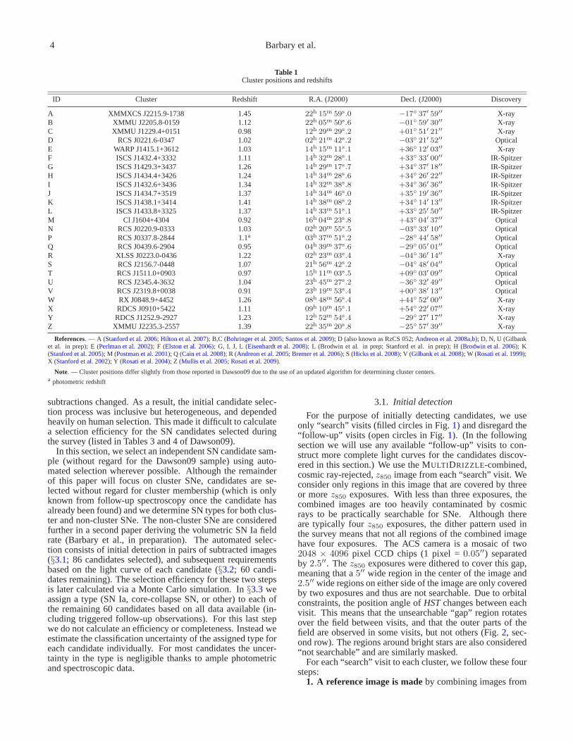
The details of theHST Cluster SN Survey are describedin Dawson09. Here, we briefly summarize the survey andhighlight the details relevant to the rate calculation. Thesur-vey targeted 25 massive galaxy clusters in a rolling searchbetween July 2005 and December 2006. Clusters were se-lected from X-ray, optical and IR surveys and cover the red-shift range0.9 < z < 1.45. Twenty-four of the clusters havespectroscopically confirmed redshifts and the remaining clus-ter has a photometric redshift estimate. Cluster positions, red-shifts and discovery methods are listed in Table1. Note thatcluster positions differ slightly from those reported in Daw-son09 due to the use of an updated algorithm for determiningcluster centers.

During the survey, each cluster was observed once every 20to 26 days during itsHST visibility window (typically fourto seven months). Figure1 shows the dates of visits to eachcluster. Each visit consisted of four exposures in the F850LPfilter (hereafterz850). Most visits also included a fifth expo-sure in the F775W filter (hereafteri775). We revisited clustersD, N, P, Q, R and Z towards the end of the survey when theybecame visible again.

Immediately following each visit, the fourz850 expo-sures were cosmic ray-rejected and combined using MUL-TIDRIZZLE (Fruchter & Hook 2002; Koekemoer et al. 2002)and searched for supernovae. Following the technique em-ployed in the earliest Supernova Cosmology Project searches(Perlmutter et al. 1995, 1997), we used the initial visit as areference image, flagged candidates with software and thenconsidered them by eye. Likely supernovae were followedup spectroscopically using pre-scheduled time on the Keck,VLT and Subaru telescopes. For nearly all SN candidates,either a live SN spectrum or host galaxy spectrum was ob-tained. In many cases, spectroscopy of cluster galaxies wasobtained contemporaneously using slit masks. Candidatesdeemed likely to be at higher redshift (z > 1) were also ob-served with the NICMOS camera onHST, but these data arenot used in this work.

A number of visits were contingent on the existence of anactive SN. At the end of a cluster’s visibility window, the lasttwo scheduled visits were cancelled if there was no live SNpreviously discovered. This is because a SN discovered onthe rise in either of the last two visits could not be followedlong enough to obtain a cosmologically useful light curve. Inaddition, supplementary visits between pre-scheduled visitswere occasionally added to provide more complete light curveinformation for SNe (in the case of clusters A, C, Q, and U).We call all visits contingent on the existence of an active SN“follow-up” visits (designated by open circles in Fig.1).

3. SUPERNOVA SELECTION

During the survey, our aim was to find as many supernovaeas possible and find them as early as possible in order to trig-ger spectroscopic and NICMOS followup. Thus, softwarethresholds for flagging candidates for consideration were setvery low, and all possible supernovae were carefully consid-ered by a human screener. Over the course of the survey,thresholds were changed and the roster of people scanning the

4 Barbary et al.

Table 1Cluster positions and redshifts

ID Cluster Redshift R.A. (J2000) Decl. (J2000) Discovery

A XMMXCS J2215.9-1738 1.45 22h 15m 59s.0 −17 37′ 59′′ X-rayB XMMU J2205.8-0159 1.12 22h 05m 50s.6 −01 59′ 30′′ X-rayC XMMU J1229.4+0151 0.98 12h 29m 29s.2 +01 51′ 21′′ X-rayD RCS J0221.6-0347 1.02 02h 21m 42s.2 −03 21′ 52′′ OpticalE WARP J1415.1+3612 1.03 14h 15m 11s.1 +36 12′ 03′′ X-rayF ISCS J1432.4+3332 1.11 14h 32m 28s.1 +33 33′ 00′′ IR-SpitzerG ISCS J1429.3+3437 1.26 14h 29m 17s.7 +34 37′ 18′′ IR-SpitzerH ISCS J1434.4+3426 1.24 14h 34m 28s.6 +34 26′ 22′′ IR-SpitzerI ISCS J1432.6+3436 1.34 14h 32m 38s.8 +34 36′ 36′′ IR-SpitzerJ ISCS J1434.7+3519 1.37 14h 34m 46s.0 +35 19′ 36′′ IR-SpitzerK ISCS J1438.1+3414 1.41 14h 38m 08s.2 +34 14′ 13′′ IR-SpitzerL ISCS J1433.8+3325 1.37 14h 33m 51s.1 +33 25′ 50′′ IR-SpitzerM Cl J1604+4304 0.92 16h 04m 23s.8 +43 04′ 37′′ OpticalN RCS J0220.9-0333 1.03 02h 20m 55s.5 −03 33′ 10′′ OpticalP RCS J0337.8-2844 1.1a 03h 37m 51s.2 −28 44′ 58′′ OpticalQ RCS J0439.6-2904 0.95 04h 39m 37s.6 −29 05′ 01′′ OpticalR XLSS J0223.0-0436 1.22 02h 23m 03s.4 −04 36′ 14′′ X-rayS RCS J2156.7-0448 1.07 21h 56m 42s.2 −04 48′ 04′′ OpticalT RCS J1511.0+0903 0.97 15h 11m 03s.5 +09 03′ 09′′ OpticalU RCS J2345.4-3632 1.04 23h 45m 27s.2 −36 32′ 49′′ OpticalV RCS J2319.8+0038 0.91 23h 19m 53s.4 +00 38′ 13′′ OpticalW RX J0848.9+4452 1.26 08h 48m 56s.4 +44 52′ 00′′ X-rayX RDCS J0910+5422 1.11 09h 10m 45s.1 +54 22′ 07′′ X-rayY RDCS J1252.9-2927 1.23 12h 52m 54s.4 −29 27′ 17′′ X-rayZ XMMU J2235.3-2557 1.39 22h 35m 20s.8 −25 57′ 39′′ X-ray

References. — A (Stanford et al. 2006; Hilton et al. 2007); B,C (Bohringer et al. 2005; Santos et al. 2009); D (also known as RzCS 052;Andreon et al. 2008a,b); D, N, U (Gilbanket al. in prep); E (Perlman et al. 2002); F (Elston et al. 2006); G, I, J, L (Eisenhardt et al. 2008); L (Brodwin et al. in prep; Stanford et al. in prep); H (Brodwin et al. 2006); K(Stanford et al. 2005); M (Postman et al. 2001); Q (Cain et al. 2008); R (Andreon et al. 2005; Bremer et al. 2006); S (Hicks et al. 2008); V (Gilbank et al. 2008); W (Rosati et al. 1999);X (Stanford et al. 2002); Y (Rosati et al. 2004); Z (Mullis et al. 2005; Rosati et al. 2009).

Note. — Cluster positions differ slightly from those reported in Dawson09 due to the use of an updated algorithm for determining cluster centers.a photometric redshift

subtractions changed. As a result, the initial candidate selec-tion process was inclusive but heterogeneous, and dependedheavily on human selection. This made it difficult to calculatea selection efficiency for the SN candidates selected duringthe survey (listed in Tables 3 and 4 of Dawson09).

In this section, we select an independent SN candidate sam-ple (without regard for the Dawson09 sample) using auto-mated selection wherever possible. Although the remainderof this paper will focus on cluster SNe, candidates are se-lected without regard for cluster membership (which is onlyknown from follow-up spectroscopy once the candidate hasalready been found) and we determine SN types for both clus-ter and non-cluster SNe. The non-cluster SNe are consideredfurther in a second paper deriving the volumetric SN Ia fieldrate (Barbary et al., in preparation). The automated selec-tion consists of initial detection in pairs of subtracted images(§3.1; 86 candidates selected), and subsequent requirementsbased on the light curve of each candidate (§3.2; 60 candi-dates remaining). The selection efficiency for these two stepsis later calculated via a Monte Carlo simulation. In§3.3 weassign a type (SN Ia, core-collapse SN, or other) to each ofthe remaining 60 candidates based on all data available (in-cluding triggered follow-up observations). For this last stepwe do not calculate an efficiency or completeness. Instead weestimate the classification uncertainty of the assigned type foreach candidate individually. For most candidates the uncer-tainty in the type is negligible thanks to ample photometricand spectroscopic data.

3.1. Initial detection

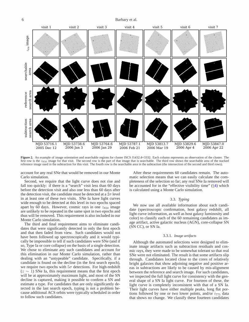
For the purpose of initially detecting candidates, we useonly “search” visits (filled circles in Fig.1) and disregard the“follow-up” visits (open circles in Fig.1). (In the followingsection we will use any available “follow-up” visits to con-struct more complete light curves for the candidates discov-ered in this section.) We use the MULTI DRIZZLE-combined,cosmic ray-rejected,z850 image from each “search” visit. Weconsider only regions in this image that are covered by threeor morez850 exposures. With less than three exposures, thecombined images are too heavily contaminated by cosmicrays to be practically searchable for SNe. Although thereare typically fourz850 exposures, the dither pattern used inthe survey means that not all regions of the combined imagehave four exposures. The ACS camera is a mosaic of two2048 × 4096 pixel CCD chips (1 pixel =0.05′′) separatedby 2.5′′. Thez850 exposures were dithered to cover this gap,meaning that a5′′ wide region in the center of the image and2.5′′ wide regions on either side of the image are only coveredby two exposures and thus are not searchable. Due to orbitalconstraints, the position angle ofHSTchanges between eachvisit. This means that the unsearchable “gap” region rotatesover the field between visits, and that the outer parts of thefield are observed in some visits, but not others (Fig.2, sec-ond row). The regions around bright stars are also considered“not searchable” and are similarly masked.

For each “search” visit to each cluster, we follow these foursteps:

1. A reference image is madeby combining images from

The SN Ia Rate in High-Redshift Galaxy Clusters 5

53600 53700 53800 53900 54000modified julian date

ABCDEFGHIJKL

MNPQRSTUVWXYZ

clu

ster

1 Jul 05 1 Oct 05 1 Jan 06 1 Apr 06 1 Jul 06 1 Oct 06

calendar date

Figure 1. Dates of visits to each cluster. All visits includedz850 exposures(usually four). Most visits also included onei775 exposure. Filled circles in-dicate “search” visits (used for finding SNe). Open circles indicate “follow-up” visits (contingent on the existence of an active SN candidate). Clusters D,N, P, Q and R were re-visited once towards the end of the survey, with addi-tional follow-up visits devoted to clusters in which promising SN candidateswere found (N, Q, R).

other visits to the cluster. All visits that are either 50 or moredays before the search epoch or 80 or more days after thesearch epoch are included. If there are no epochs outside this130 day range, the range is narrowed symmetrically until oneepoch qualifies. Masked pixels in each visit’s image do notcontribute to the stacked reference image (Fig.2, third row).

2. A subtracted image is madeby subtracting the stackedreference image from the search epoch image. A map of thesky noise level in the subtraction is made by considering thenoise level of the search epoch image and the noise level ofeach reference image contributing to a given region. Any areamasked in either the search epoch or stacked reference imageis masked in the subtracted image (Fig.2, fourth row).

3. Candidates in the subtraction are identified by soft-ware. To be flagged, a candidate must have three contiguouspixels with a flux 3.4 times the local sky noise level in thesubtraction (as determined by the sky noise map above). Onceflagged, it must fulfill the following four requirements:

• MULTI DRIZZLE-combined image: A total signal-to-noise ratio (including sky and Poisson noise) of 5 ormore in a 3 pixel radius aperture.

• MULTI DRIZZLE-combined image: A total signal-to-noise ratio of 1.5 or more in a 10 pixel radius aperture.

• Individual exposures: A signal-to-noise ratio of 1 or

Table 2Light Curve Requirements

Requirement Candidates Remaining

Before light curve requirements 86Positivei775 flux (if observed ini775) 812σ Detection in surrounding epochs 73If declining, Require two5σ detections 60

greater in a 3 pixel radius aperture in three or more in-dividual exposures.

• Individual exposures: A candidate cannot have an indi-vidual exposure with a flux more than20σ greater thanthe flux in the lowest flux exposureand a second indi-vidual exposure with flux more than10σ greater thanthe flux in the lowest flux exposure.

The first requirement is designed to eliminate low significancedetections on bright galaxies. The second requirement helpseliminate dipoles on bright galaxy cores caused by slight im-age misalignment. The third and fourth requirements areaimed at false detections due to cosmic ray coincidence. Theyrequire the candidate to be detected in most of the exposuresand allow no more than one exposure to be greatly affected bya cosmic ray. On the order of five to ten candidates per sub-traction pass all the requirements, resulting in approximately1000 candidates automatically flagged across the 155 searchvisits.

4. Each candidate is evaluated by eye in the subtraction.Because the position angle changes between each epoch, theorientation of stellar diffraction spikes changes, causing themajority of the false detections. These are easy to detect andeliminate by eye. Occasionally there are mis-subtractionsonthe cores of bright galaxies that pass the above requirements.Only completely unambiguous false detections are eliminatedin this step. If there is any possibility the candidate is a realSN, it is left in the sample for further consideration.

After carrying out the above four steps for all 155 searchvisit, 86 candidates remain. At this point, candidates havebeen selected based only on information from a singlez850subtraction.

3.2. Lightcurve Requirements

The 86 remaining candidates still include a considerablenumber of non-SNe. We wish to trim the sample down asmuch as possible in an automated way, so that we can easilycalculate the efficiency of our selection. For each candidate,we now make three further automated requirements based oni775 data (if available) and the shape of thez850 light curve.The requirements and number of candidates remaining aftereach requirement are summarized in Table2.

First, we require that ifi775 data exists for the epoch inwhich the candidate was detected, there be positive flux in a2 pixel radius aperture at the candidate location in thei775image. From our SN light curve simulations, we find that vir-tually all SNe should pass (near maximum light there is typ-ically enough SN flux in thei775 filter to result in a positivetotal flux, even with large negative sky fluctuations). Mean-while, about half of the cosmic rays located far from galaxieswill fail this test (due to negative sky fluctuations). If there isno i775 data for the detection epoch, this requirement is notapplied. Even though nearly all SNe are expected to pass, we

6 Barbary et al.

sub

tract

ion

searc

h a

rea

refe

ren

cese

arc

h a

rea

searc

hab

leare

az 8

50 i

mag

evisit 1

MJD 53716.12005 Dec 12

visit 2

MJD 53738.62006 Jan 3

visit 3

MJD 53764.62006 Jan 29

visit 4

MJD 53787.12006 Feb 21

visit 5

MJD 53813.72006 Mar 19

visit 6

MJD 53829.62006 Apr 4

visit 7

MJD 53847.02006 Apr 22

Figure 2. An example of image orientation and searchable regions for cluster ISCS J1432.4+3332. Each column represents an observation of the cluster. Thefirst row is thez850 image for that visit. The second row is the part of that image that is searchable. The third row shows the searchable area of the stackedreference image used in the subtraction for this visit. The fourth row is the searchable area in the subtraction (the intersection of the second and third rows).

account for any real SNe that would be removed in our MonteCarlo simulation.

Second, we require that the light curve does not rise andfall too quickly: if there is a “search” visit less than 60 daysbefore the detection visit and also one less than 60 days afterthe detection visit, the candidate must be detected at a2σ levelin at least one of these two visits. SNe Ia have light curveswide enough to be detected at this level in two epochs spacedapart by 60 days. However, cosmic rays in onez850 imageare unlikely to be repeated in the same spot in two epochs andthus will be removed. This requirement is also included in ourMonte Carlo simulation.

The third and final requirement aims to eliminate candi-dates that were significantly detected in only the first epochand that then faded from view. Such candidates would nothave been followed up spectroscopically and it would typi-cally be impossible to tell if such candidates were SNe (and ifso, Type Ia or core collapse) on the basis of a single detection.We chose to eliminate any such candidates and account forthis elimination in our Monte Carlo simulation, rather thandealing with an “untypeable” candidate. Specifically, if acandidate is found on the decline (in the first search epoch),we require two epochs with5σ detections. For high-redshift(z ∼ 1) SNe Ia, this requirement means that the first epochwill be at approximately maximum light, and most of the SNdecline is captured, making it possible to confirm a SN andestimate a type. For candidates that are only significantly de-tected in the last search epoch, typing is not a problem be-cause additional ACS orbits were typically scheduled in orderto follow such candidates.

After these requirements 60 candidates remain. The auto-matic selection means that we can easily calculate the com-pleteness of the selection so far; any real SNe Ia removed willbe accounted for in the “effective visibility time” (§4) whichis calculated using a Monte Carlo simulation.

3.3. Typing

We now use all available information about each candi-date (spectroscopic confirmation, host galaxy redshift, alllight curve information, as well as host galaxy luminosity andcolor) to classify each of the 60 remaining candidates as im-age artifact, active galactic nucleus (AGN), core-collapse SN(SN CC), or SN Ia.

3.3.1. Image artifacts

Although the automated selections were designed to elim-inate image artifacts such as subtraction residuals and cos-mic rays, they were made to be somewhat tolerant so that realSNe were not eliminated. The result is that some artifacts slipthrough. Candidates located close to the cores of relativelybright galaxies that show adjoining negative and positive ar-eas in subtractions are likely to be caused by mis-alignmentbetween the reference and search image. For such candidates,we inspected the full light curve for consistency with the gen-eral shape of a SN Ia light curve. For fourteen of these, thelight curve is completely inconsistent with that of a SN Ia.Their light curves have either multiple peaks, long flat por-tions followed by one or two lower points, and/ori775 datathat shows no change. We classify these fourteen candidates

The SN Ia Rate in High-Redshift Galaxy Clusters 7

as subtraction residuals with negligible classification uncer-tainty (very unlikely that any are SNe Ia).

Candidates where one or two of the fourz850 exposureswas clearly affected by a cosmic ray or hot pixel may be falsedetections. These can pass the automated cosmic ray rejec-tion when they occur on a galaxy. For two such candidates,we used the lack of any change in thei775 light curve to ruleout a SN Ia: fitting SN templates with a range of redshiftsand extinctions resulted in observedi775 fluxes too low by4σ or more, given thez850 increase. One other candidate,SCP06W50, is less certain. It was discovered in the last visitto the cluster, making it difficult to constrain a template lightcurve. There is clearly a hot pixel or cosmic ray in onez850exposure, but there appears to be some excess flux in the otherthree exposures as well. Also, there is a point-source like de-tection ini775, but offset∼1.2 pixels from thez850 detection.While thei775 detection may also be a cosmic ray, it is pos-sible that this candidate is a SN caught very early. The el-liptical “host” galaxy was not observed spectroscopically, butwe estimate its redshift to be0.60 < z < 0.85 based on thecolor of i775 − z850 = 0.55 and stellar population models ofBruzual & Charlot(2003, hereafter BC03).

Of the 17 total candidates classified as image artifacts,SCP06W50 is the only one with significant uncertainty. How-ever, this uncertainty does not affect the cluster SN Ia rateasthe host galaxy is clearly in the cluster foreground.

3.3.2. AGN

Candidates positioned directly on the cores of their hostgalaxies may be AGN. Four such candidates were spec-troscopically confirmed as AGN: SCP06L22 (z = 1.369),SCP06V6 (z = 0.903) and SCP05X13 (z = 1.642) andSCP06U3 (z = 1.534). A fifth candidate, SCP06F3, is spec-troscopically consistent with an AGN atz = 1.21, but is lesscertain (see spectroscopy reported inMorokuma et al. 2010).SCP06L22, SCP05X13, SCP06U3 and SCP06F3 also havelight curves that are clearly inconsistent with SNe Ia (observerframe rise times of 100 days or more, or declining phases pre-ceding rising phases). Of the “on core” candidates that werenot observed spectroscopically, five exhibit light curves thatdecline before rising or have rise times of 100 days or more. Asixth candidate, SCP06Z51 exhibited slightly varying fluxesthat could be due to either subtraction residuals or an AGN.However, its light curve is clearly inconsistent with a SN Ia,especially considering the apparent size, magnitude and colorof the host galaxy. Summarizing, there are 11 “on-core” can-didates certain not to be SNe Ia.

Three other “on-core” candidates are also consideredlikely AGN on the basis of their light curves: SCP06Z50,SCP06U50 and SCP06D51. These three candidates areshown in Fig.3. SCP06Z50 (Fig.3, top left), has a rise-fall behavior in the first threez850 observations of its lightcurve thatcouldbe consistent with a SN Ia light curve. How-ever, given that the host galaxy is likely atz . 1 based on itsmagnitude and color, the SN would be fainter than a normalSN Ia by 1 magnitude or more. Considering the proximityto the galaxy core and the additional variability seen in thelast two observations, SCP06Z50 is most likely an AGN. Thelight curve of candidate SCP06U50 (Fig.3, top right) alsoexhibits a rise-fall that could be consistent with a supernovalight curve. However, its host is morphologically ellipticaland likely atz . 0.7 based on its color. Atz . 0.7, a SN Iawould have to be very reddened (E(B − V ) & 1) to matchthe color and magnitude of the SCP06U50 light curve. As

this is very unlikely (considering that the elliptical hostlikelycontains little dust), we conclude that SCP06U50 is also mostlikely an AGN. Finally, SCP06D51 (Fig.3, bottom left) wasdiscovered in the last visit, on the core of a spiral galaxy. Weclassify it as an AGN based on the earlier variability in thelight curve. As these galaxies are all most likely in the clus-ter foregrounds, even the small uncertainty in these classifica-tions is not a concern for the cluster rate calculation here.

Note that one of the candidates classified here as a clearAGN, SCP06U6, was reported as a SN with unknown red-shift by Dawson09, due to the fact that spectroscopy revealedno evidence of an AGN. However, it is on the core of a com-pact galaxy, and has a clear& 100 day rise in bothz850 andi775 (Fig. 3, bottom right). While it could possibly be a verypeculiar SN with a long rise time, what is important for thisanalysis is that it is clearly not a SN Ia.

3.3.3. Supernovae

After removing 17 image artifacts and 14 AGN, 29 candi-dates remain (listed in Table3). One of these is the peculiartransient SCP 06F6 (also known as SN SCP06F6) reported byBarbary et al.(2009). Various explanations have been con-sidered by, e.g.,Gansicke et al.(2009), Soker et al.(2010)and Chatzopoulos et al.(2009). It appears that SCP 06F6may be a rare type of supernova, with redshiftz = 1.189(Quimby et al. 2009). While its precise explanation is still un-certain, SCP 06F6 is clearly not a SN Ia, so we don’t considerit further here.

Note that Table3 contains 10 fewer candidates than thelist presented by Dawson09. This is unsurprising; here wehave intentionally used a stricter selection than in the origi-nal search, the source for the Dawson09 sample. Still, afterfinalizing our selection method we checked that there were nounexpected discrepancies. Five of the Dawson09 candidates(SCP06B4, SCP06U2, SCP06X18, SCP06Q31, SCP06T1)fell just below either the detection or signal-to-noise thresh-olds in our selection. These were found in the original searchbecause detection thresholds were set slightly lower, and be-cause the images were sometimes searched in several differentways. For example, in the original search SCP06B4 was onlyfound by searching ani775 subtraction. Two Dawson09 can-didates (SCP05D55, SCP06Z52) were found too far on thedecline and failed the light curve requirements (§3.2). ThreeDawson09 candidates (SCP06X27, SCP06Z13, SCP06Z53)were found while searching in “follow-up” visits, which werenot searched here. SCP06U6 passed all requirements, but isclassified here as an AGN, as noted above. With the excep-tion of SCP06U6, all of these candidates are likely to be su-pernovae (mostly core collapse). However, the types of candi-dates that did not pass our requirements are not of concern forthis analysis. Finally, SCP06M50 was not reported in Daw-son09, but is classified here as a SN, although a highly uncer-tain one (discussed in detail in§3.3.4).

Thanks to the extensive ground-based spectroscopic fol-lowup campaign, we were able to obtain spectroscopic red-shifts for 25 of the 29 SNe. The redshift reported in Table3is derived from the SN host galaxy for all but one candidate(SCP06C1) where the redshift is from the SN spectrum itself.Of the 25 candidates with redshifts, eight are in clusters and17 are in the field. Note that this high spectroscopic com-pleteness is particularly important for determining the clusteror non-cluster status of each SN, which directly affects thedetermination of the cluster SN Ia rate. The possible clus-ter memberships of the four candidates lacking redshifts are

8 Barbary et al.

SCP06Z50AGN

1.0" E

N

ref new sub

4.6

4.8

5.0

5.2

5.4

z850

50 1007.2

7.4

7.6

7.8

8.0

i775

350 400 450

SCP06U50AGN

ref new sub

7.8

8.0

8.2

8.4

8.6 z850

400 450 50013.6

13.8

14.0

14.2

14.4 i775

SCP06D51AGN

ref new sub

3.94.04.14.24.34.44.54.64.7

z850

50 100 150 2003.8

4.0

4.2

4.4

4.6 i775

450

SCP06U6AGN

ref new sub

0.6

0.8

1.0

1.2

1.4z850

400 450 500 550

1.21.41.61.82.02.2 i775

MJD - 53500 MJD - 53500

Figure 3. Images and light curves of four of the 14 candidates classifiedas AGN. For each candidate, the upper left panel shows the two-color stacked image(i775 andz850) of the host galaxy, with the position of the transient indicated. The three smaller panels below the stacked image show thereference, new, andsubtracted images for the discovery visit. The right panel shows the light curve at the SN position (including host galaxylight) in thez850 (top) andi775 (bottom)bands. The y axes have units of counts per second in a3 pixel radius aperture. The effective zeropoints are 23.94 and 25.02 forz850 andi775, respectively. Thediscovery visit is indicated with an arrow in thez850 plot.

discussed below.We determine the type of each of the 29 supernovae using

a combination of methods in order to take into account allavailable information for each supernova. This includes (a)spectroscopic confirmation, (b) the host galaxy environment,and (c) the SN light curve. To qualify the confidence of eachsupernova’s type, we rank the type as “secure,” “probable,”or“plausible”:

Secure SN Ia:Has spectroscopic confirmation orbothof thefollowing: (1) an early-type host galaxy with no recentstar formation and (2) a light curve with shape, colorand magnitude consistent with SNe Ia and inconsistentwith other types.

Probable SN Ia: Fulfills either the host galaxy requirementor the light curve requirement, but not both.

Plausible SN Ia: The light curve is indicative of a SN Ia, butthere is not enough data to rule out other types.

Secure SN CC:Has spectroscopic confirmation (note thatthere are no such candidates in this sample).

Probable SN CC: The light curve is consistent with a core-collapse SN and inconsistent with a SN Ia.

Plausible SN CC: Has a light curve indicative of a core-collapse SN, but not inconsistent with a SN Ia.

This ranking system is largely comparable to the “gold,” “sil-ver,” “bronze” ranking system ofStrolger et al.(2004), exceptthat we do not use their “UV deficit” criterion. This is becauseour data do not include the bluer F606W filter, and becauseSNe Ia and CC are only distinct in UV flux for a relativelysmall window early in the light curve. Below, we discuss indetail the three typing methods used.

(a) Spectroscopic confirmation:During the survey, sevencandidates were spectroscopically confirmed as SNe Ia (Daw-son09,Morokuma et al. 2010). These seven (three of whichare in clusters) are designated with an “a” in the “typing” col-umn of Table3. All seven candidates have a light curve shape,absolute magnitude and color consistent with a SN Ia. Al-though the spectroscopic typing by itself has some degree ofuncertainty, the corroborating evidence from the light curvemakes these “secure” SNe Ia.

(b) Early-type host galaxy: The progenitors of core-collapse SNe are massive stars (> 8M⊙) with main sequencelifetimes of< 40 Myr. Thus, core-collapse SNe only occur ingalaxies with recent star formation. Early-type galaxies,hav-ing typically long ceased star formation, overwhelmingly hostType Ia SNe (e.g.,Cappellaro et al. 1999; Hamuy et al. 2000).In fact, in an extensive literature survey of core-collapseSNereported in early-type hosts,Hakobyan et al.(2008) foundthat only three core-collapse SNe have been recorded in early-type hosts, and that the three host galaxies in question had ei-ther undergone a recent merger or were actively interacting.In all three cases there are independent indicators of recentstar formation. Therefore, in the cases where the host galaxymorphology, photometric color, and spectrum all indicate anearly-type galaxy with no signs of recent star formation or in-teraction, we can be extremely confident that the SN type is Ia.These cases are designated by a “b” in the “typing” column ofTable3. We emphasize that in all of these cases, spectroscopyreveals no signs of recent star formation and there are no vi-sual or morphological signs of interaction. (See Meyers10 fordetailed studies of these SN host galaxy properties.)

(c) Light curve: SNe Ia can be distinguished from mostcommon types of SNe CC by some combination of light curveshape, color, and absolute magnitude. We compare the lightcurve of each candidate to template light curves for SN Ia

The SN Ia Rate in High-Redshift Galaxy Clusters 9

Table 3Supernovae

ID Nickname R.A. (J2000) Decl. (J2000) z SN Type Confidence Typing

Cluster Members

SN SCP06C1 Midge 12h 29m 33s.012 +01 51′ 36′′.67 0.98 Ia secure a,cSN SCP05D0 Frida 02h 21m 42s.066 −03 21′ 53′′.12 1.014 Ia secure a,b,cSN SCP06F12 Caleb 14h 32m 28s.748 +33 32′ 10′′.05 1.11 Ia probable cSN SCP06H5 Emma 14h 34m 30s.139 +34 26′ 57′′.29 1.231 Ia secure b,cSN SCP06K18 Alexander 14h 38m 10s.663 +34 12′ 47′′.19 1.412 Ia probable bSN SCP06K0 Tomo 14h 38m 08s.366 +34 14′ 18′′.08 1.416 Ia secure b,cSN SCP06R12 Jennie 02h 23m 00s.082 −04 36′ 03′′.04 1.212 Ia secure b,cSN SCP06U4 Julia 23h 45m 29s.429 −36 32′ 45′′.73 1.05 Ia secure a,c

Cluster Membership Uncertain

SN SCP06E12 Ashley 14h 15m 08s.141 +36 12′ 42′′.94 · · · Ia plausible cSN SCP06N32 · · · 02h 20m 52s.368 −03 34′ 13′′.32 · · · CC plausible c

Not Cluster Members

SN SCP06A4 Aki 22h 16m 01s.077 −17 37′ 22′′.09 1.193 Ia probable cSN SCP06B3 Isabella 22h 05m 50s.402 −01 59′ 13′′.34 0.743 CC probable cSN SCP06C0 Noa 12h 29m 25s.654 +01 50′ 56′′.58 1.092 Ia secure b,cSN SCP06C7 · · · 12h 29m 36s.517 +01 52′ 31′′.47 0.61 CC probable cSN SCP05D6 Maggie 02h 21m 46s.484 −03 22′ 56′′.18 1.314 Ia secure b,cSN SCP06F6 · · · 14h 32m 27s.394 +33 32′ 24′′.83 1.189 non-Ia secure aSN SCP06F8 Ayako 14h 32m 24s.525 +33 33′ 50′′.75 0.789 CC probable cSN SCP06G3 Brian 14h 29m 28s.430 +34 37′ 23′′.13 0.962 Ia plausible cSN SCP06G4 Shaya 14h 29m 18s.743 +34 38′ 37′′.38 1.35 Ia secure a,b,cSN SCP06H3 Elizabeth 14h 34m 28s.879 +34 27′ 26′′.61 0.85 Ia secure a,cSN SCP06L21 · · · 14h 33m 58s.990 +33 25′ 04′′.21 · · · CC plausible cSN SCP06M50 · · · 16h 04m 25s.300 +43 04′ 51′′.85 · · · · · · · · · · · ·

SN SCP05N10 Tobias 02h 20m 52s.878 −03 33′ 40′′.20 0.203 CC plausible cSN SCP06N33 Naima 02h 20m 57s.699 −03 33′ 23′′.97 1.188 Ia probable cSN SCP05P1 Gabe 03h 37m 50s.352 −28 43′ 02′′.66 0.926 Ia probable cSN SCP05P9 Lauren 03h 37m 44s.512 −28 43′ 54′′.58 0.821 Ia secure a,cSN SCP06U7 Ingvar 23h 45m 33s.867 −36 32′ 43′′.48 0.892 CC probable cSN SCP06X26 Joe 09h 10m 37s.889 +54 22′ 29′′.07 1.44 Ia plausible cSN SCP06Z5 Adrian 22h 35m 24s.966 −25 57′ 09′′.61 0.623 Ia secure a,c

Note. — Typing: (a) Spectroscopic confirmation. (b) Host is morphologically early-type, with no signs of recent star formation. (c) Light curve shape, color, magnitude consistentwith type. We do not assign a type for SCP06M50 because there is significant uncertainty that the candidate is a SN at all.

and various SN CC subtypes to test if the candidate couldbe a SN Ia or a SN CC. For candidates lacking both spec-troscopic confirmation and an elliptical host galaxy, if thereis sufficient light curve data to rule out all SN CC subtypes,the candidate is considered a “probable” SN Ia. If SN Ia canbe ruled out, it is considered a “probable” SN CC. If neitherSN Ia nor SN CC can be ruled out, the candidate is consid-ered a “plausible” SN Ia or SN CC based on how typicalthe candidate’s absolute magnitude and/or color would be ofeach type. This approach can be viewed as a qualitative ver-sion of the pseudo-Bayesian light curve typing approachesof, e.g., Kuznetsova & Connolly(2007); Kuznetsova et al.(2008); Poznanski et al.(2007a,b). SNe classified as “prob-able” here would likely have a Bayesian posterior probabilityapproaching1, while “plausible” SNe would have an inter-mediate probability (likely between 0.5 and 1.0). We con-sciously avoid the full Bayesian typing approach because itcan obscure large uncertainties in the priors such as lumi-nosity distributions, relative rates, light curve shapes,andSN subtype fractions. Also, the majority of our candidateshave more available light curve information than those ofKuznetsova et al.(2008) andPoznanski et al.(2007b), mak-ing a calculation of precise classification uncertainty less nec-essary. In general, classification uncertainty from light curve

fitting is not a concern for the cluster rate calculation as mostcluster-member candidates are securely typed using methods(a) and/or (b), above. It is more of a concern for the volumet-ric field rate calculation based on the non-cluster candidates(Barbary et al., in preparation), though the uncertainty inthefield rate is still dominated by Poisson error.

For each candidate we fit template light curves for SN Ia,Ibc, II-P, II-L, and IIn. We use absolute magnitude and coloras a discriminant by limiting the allowed fit ranges accord-ing to the known distributions for each subtype. For SN Iawe start with the spectral time series template ofHsiao et al.(2007), while for the core-collapse types we use templates ofNugent et al.(2002)28. Each spectral time series is redshiftedto the candidate redshift and warped according to the desiredcolor. Observer-frame template light curves are then gener-ated by synthetic photometry in thei775 andz850 filters. Themagnitude, color, date of maximum light, and galaxy flux ini775 andz850 are allowed to vary to fit the light curve data.For the SN Ia template, the linear timescale or “stretch” (e.g.,Perlmutter et al. 1997; Guy et al. 2005) is also allowed to varywithin the range0.6 < s < 1.3. We constrain the abso-lute magnitude for each subtype to the range observed by

28 Seehttp://supernova.lbl.gov/∼nugent/nugenttemplates.html.

10 Barbary et al.

Table 4SN light curve template parameter ranges

SN type Template ObservedMB E(B − V ) s

Ia Hsiao −17.5 –−20.1 −0.2 – 0.6 0.6 – 1.3Ibc Nugent −15.5 –−18.5 −0.1 – 0.5 1.0II-L Nugent −16.0 –−19.0 −0.1 – 0.5 1.0II-P Nugent −15.5 –−18.0 −0.1 – 0.5 1.0IIn Nugent −15.5 –−19.1 −0.1 – 0.5 1.0

Li et al. (2010); Our allowed range fully encompasses theirobserved luminosity functions (uncorrected for extinction) fora magnitude-limited survey for each subtype. We correct fromtheir assumed value ofH0 = 73 km s−1 Mpc−1 to our as-sumed value ofH0 = 70 km s−1 Mpc−1 and K-correctfrom R to B band. To avoid placing too strict of an up-per limit on SN CC brightness, we use the bluest maximum-light spectrum available whenK-correcting (e.g., for SN Ibcwe use a bluer spectrum than that ofNugent et al.(2002), asbluer SNe Ibc have been observed). The resulting allowedMB range for each subtype is shown in Table4. Note thatthe range for Ibc does not include ultra-luminous SNe Ic(such as those in the luminosity functions ofRichardson et al.(2002)) as none were discovered byLi et al. (2010). Whilesuch SNe can mimic a SN Ia photometrically, theLi et al.(2010) results indicate that they are intrinsically rare, andevenRichardson et al.(2002) show that they make up at most∼20% of all SNe Ibc. Still, we keep in mind that even can-didates compatible only with our SN Ia template and incom-patible with SN CC templates may in fact be ultra-luminousSNe Ic, though the probability is low. This is why any candi-date typed based on light curve alone has a confidence of atmost “probable,” rather than “secure.” The allowed ranges of“extinction,”E(B−V ), are also shown in Table4. For SN Ia,E(B−V ) is the difference inB−V color from theHsiao et al.(2007) template. As the observed distribution of SNe includesSNe bluer than this template, SNe Ia as blue asE(B − V ) =−0.2 are allowed. Given anE(B − V ), the spectral tem-plate is warped according to theSALT color law (Guy et al.2005), with an effectiveRB = 2.28 (Kowalski et al. 2008).For SN CC templates, extinction as low asE(B−V ) = −0.1is allowed to reflect the possibility of SNe that are intrinsicallybluer than theNugent et al.(2002) templates. Templates arethen warped using aCardelli et al.(1989) law withRB = 4.1.Extinctions are limited toE(B − V ) < 0.5 (implying an ex-tinction ofAB ∼ 2 magnitudes for SNe CC).

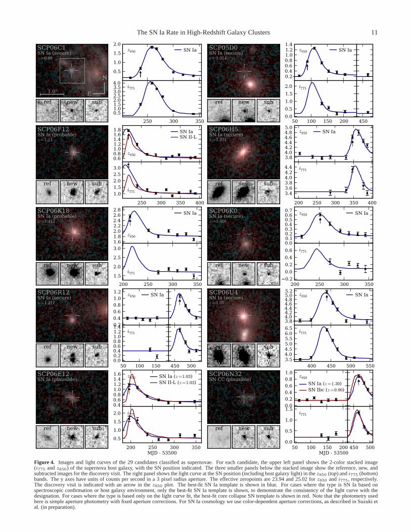
The light curve template with the largestχ2 P -value is gen-erally taken as the type. We also evaluate each fit by eye tocheck that the best-fit template adequately describes the lightcurve. Figure4 shows the best-fit template for each candidate.For candidates typed on the basis of spectroscopic confirma-tion or an elliptical host galaxy only the SN Ia template isshown. For candidates typed on the basis of the light curvealone, we show both the best-fit SN Ia and best-fit SN CCtemplates for comparison. The confidence in the best-fit tem-plate is either “probable” or “plausible” depending on howwell other templates fit: If the next-best fit has aP -value thatis smaller than10−3 × Pbest, the best-fit template is consid-ered the only acceptable fit and the confidence is “probable.”If the next-best fit has aP -value larger than10−3 × Pbest theconfidence is “plausible.” Finally, note that the photometryused here is simple aperture photometry with fixed aperturecorrections. For SN Ia cosmology we use color-dependent

aperture corrections, as described in Suzuki et al. (in prepara-tion).

3.3.4. Comments on individual SN light curves

Here we comment in greater detail on a selection of individ-ual candidates, particularly those with the greatest uncertaintyin typing. For each candidate, see the corresponding panel ofFig. 4 for an illustration of the candidate host galaxy and lightcurve.

SN SCP06E12. We were unable to obtain a host galaxyredshift due to the faintness of the host. The color of thehost galaxy is consistent with the cluster red sequence. Thecandidate light curve is consistent with a SN Ia at the clusterredshift ofz = 1.03, but is also consistent with SN II-L atz = 1.03. Different SN types provide an acceptable fit over afairly wide range of redshifts. As the SN Ia template providesa good fit with typical parameters, we classify the candidateas a “plausible” SN Ia. However, there is considerable uncer-tainty due to the uncertain redshift.

SN SCP06N32also lacks a host galaxy redshift. If thecluster redshift ofz = 1.03 is assumed, the candidate lightcurve is best fit by a SN Ibc template. A SN Ia template alsoyields an acceptable fit, but requires an unusually red colorof E(B − V ) ∼ 0.6. Given the best-fits andMB values,the candidate would have an unusually large Hubble diagramresidual of approximately−0.8 magnitudes. If the redshift isallowed to float, a SN Ia template with more typical param-eters provides an acceptable fit atz = 1.3. A SN Ibc tem-plate still provides a better fit, with the best fit redshift beingz ∼ 0.9. As SN Ibc provides a better fit in both cases, weclassify this as a “plausible” SN CC. However, there is con-siderable uncertainty in both the type and cluster membershipof this candidate.

SN SCP06A4. We note that this candidate was observedspectroscopically, as reported in Dawson09. While the spec-trum was consistent with a SN Ia, there was not enough evi-dence to conclusively assign a type. The host galaxy is mor-phologically and photometrically consistent with an early-type galaxy, but there is detected [OII], a possible indicationof star formation. We therefore rely on light curve typingfor this candidate, assigning a confidence of “probable” ratherthan “secure.”

SN SCP06G3has only sparse light curve coverage. Thebest fit template is a SN Ia withs = 1.3, E(B − V ) = 0.3andMB = −18.5, although these parameters are poorly con-strained. A large stretch and red color would not be surprisinggiven the spiral nature of the host galaxy. It is also consistentwith a II-L template, although the best fit color is unusuallyblue:E(B − V ) = −0.1. Given that SN Ia yields more “typ-ical” fit parameters and that, atz ∼ 1 a detected SN is morelikely to be Type Ia than II, we classify this as a “plausible”Type Ia, with considerable uncertainty in the type.

SN SCP06L21lacks a spectroscopic redshift, but has a dis-tinct slowly-declining light curve that rules out az > 0.6SN Ia light curve. Even the best-fit Ia template atz = 0.55,shown in Fig.4), is unusually dim (MB ≈ −17.5), makingit unlikely that the candidate is a lower-redshift SN Ia. Thelight curve is better fit by a SN II-P template (with the best-fitredshift beingz = 0.65). We therefore classify the candidateas a “probable” SN CC.

SN SCP06M50is the most questionable “SN” candidate,having no obviousi775 counterpart to the increase seen inz850. It may in fact be an image artifact or AGN. However,it appears to be off the core of the galaxy by∼2 pixels (mak-

The SN Ia Rate in High-Redshift Galaxy Clusters 11

SCP06C1SN Ia (secure)z=0.98

1.0" E

N

ref new sub

0.5

1.0

1.5

2.0z850 SN Ia

250 300 350

0.51.01.52.02.53.03.54.0

i775

SCP05D0SN Ia (secure)z=1.014

ref new sub

0.20.40.60.81.01.21.4

z850 SN Ia

50 100 150 2000.0

0.5

1.0

1.5

2.0 i775

450

SCP06F12SN Ia (probable)z=1.11

ref new sub

0.60.81.01.21.41.61.8

z850

SN IaSN II-L

250 300 350 400

1.01.52.02.53.0

i775

SCP06H5SN Ia (secure)z=1.231

ref new sub

3.84.04.24.44.64.85.0

z850 SN Ia

200 250 300 350 400

3.43.63.84.04.24.4 i775

SCP06K18SN Ia (probable)z=1.412

ref new sub

1.61.82.02.22.42.62.8

z850

SN Ia

200 250 300 350

1.5

2.0

2.5

3.0

i775

SCP06K0SN Ia (secure)z=1.416

ref new sub

0.00.10.20.30.40.50.60.7 z850 SN Ia

200 250 300 3500.2

0.0

0.2

0.4

0.6 i775

SCP06R12SN Ia (secure)z=1.212

ref new sub

0.20.40.60.81.01.2 z850 SN Ia

50 100 1500.00.20.40.60.81.01.21.4

i775

450 500

SCP06U4SN Ia (secure)z=1.05

ref new sub

3.84.04.24.44.64.85.05.2

z850 SN Ia

400 450 500 5503.54.04.55.05.56.06.5

i775

SCP06E12SN Ia (plausible)

ref new sub

0.40.60.81.01.21.41.6 z850 SN Ia (z=1.03)

SN II-L (z=1.03)

200 250 300 350

0.5

1.0

1.5

2.0 i775

SCP06N32SN CC (plausible)

ref new sub

0.00.20.40.60.81.0

z850SN Ia (z=1.30)SN Ibc (z=0.90)

50 100 150 2000.0

0.5

1.0

1.5i775

450 500MJD - 53500 MJD - 53500

Figure 4. Images and light curves of the 29 candidates classified as supernovae. For each candidate, the upper left panel shows the 2-color stacked image(i775 andz850) of the supernova host galaxy, with the SN position indicated. The three smaller panels below the stacked image show the reference, new, andsubtracted images for the discovery visit. The right panel shows the light curve at the SN position (including host galaxylight) in thez850 (top) andi775 (bottom)bands. The y axes have units of counts per second in a3 pixel radius aperture. The effective zeropoints are 23.94 and 25.02 forz850 andi775, respectively.The discovery visit is indicated with an arrow in thez850 plot. The best-fit SN Ia template is shown in blue. For cases where the type is SN Ia based onspectroscopic confirmation or host galaxy environment, only the best-fit SN Ia template is shown, to demonstrate the consistency of the light curve with thedesignation. For cases where the type is based only on the light curve fit, the best-fit core collapse SN template is shown in red. Note that the photometry usedhere is simple aperture photometry with fixed aperture corrections. For SN Ia cosmology we use color-dependent aperture corrections, as described in Suzuki etal. (in preparation).

12 Barbary et al.

SCP06A4SN Ia (probable)z=1.193

1.0" E

N

ref new sub

0.20.40.60.81.01.2 z850

SN IaSN II-L

350 400 4500.20.40.60.81.01.21.4

i775

SCP06B3SN CC (probable)z=0.743

ref new sub

0.00.20.40.60.81.0 z850 SN IIn

SN II-LSN Ia

350 400 450

0.0

0.5

1.0

1.5

2.0i775

SCP06C0SN Ia (secure)z=1.092

ref new sub

0.2

0.4

0.6

0.8

1.0

1.2z850 SN Ia

250 300 350

0.20.40.60.81.01.21.41.6

i775

SCP06C7SN CC (probable)z=0.61

ref new sub

0.60.81.01.21.4 z850 SN Ia

SN II-L

250 300

1.0

1.5

2.0

2.5

3.0i775

SCP05D6SN Ia (secure)z=1.314

ref new sub

0.4

0.6

0.8

1.0

1.2z850

SN Ia

50 100 150 2000.20.40.60.81.01.21.41.6

i775

450

SCP06F6SN non-Ia (secure)z=1.189

ref new sub

02468

101214

z850 No templatematched

250 300 350 40005

101520253035

i775

SCP06F8SN CC (probable)z=0.789

ref new sub

0.6

0.8

1.0

1.2 z850SN II-PSN Ia

250 300 350 400

1.0

1.5

2.0

2.5i775

SCP06G3SN Ia (plausible)z=0.962

ref new sub

0.0

0.5

1.0

1.5 z850 SN IaSN II-L

250 300 350

0.51.01.52.02.5 i775

SCP06G4SN Ia (secure)z=1.35

ref new sub

0.00.20.40.60.81.0

z850 SN Ia

250 300 350 4000.0

0.5

1.0

1.5 i775

SCP06H3SN Ia (secure)z=0.85

ref new sub

0.5

1.0

1.5

2.0

2.5z850 SN Ia

200 250 300 350 400

12345 i775

MJD - 53500 MJD - 53500

Figure 4. Continued

The SN Ia Rate in High-Redshift Galaxy Clusters 13

SCP06L21SN CC (plausible)

1.0" E

N

ref new sub

0.20.40.60.81.01.2

z850

SN Ia (z=0.55)SN II-P (z=0.65)

200 250 3000.5

1.0

1.5

2.0

2.5

i775

SCP06M50SN ?

ref new sub

5.4

5.6

5.8

6.0

6.2

6.4z850 SN II-L (z=0.92)

SN Ia (z=0.92)

200 250 3005.65.86.06.26.46.66.8

i775

SCP05N10SN CC (plausible)z=0.203

ref new sub

0.20.40.60.81.01.2

z850

No templatematched

50 100 150 200

0.2

0.4

0.6

0.8

1.0

i775

450 500

SCP06N33SN Ia (probable)z=1.188

ref new sub

0.00.20.40.60.81.01.2

z850 SN IaSN II-L

50 100 150 2000.0

0.5

1.0

1.5 i775

450 500

SCP05P1SN Ia (probable)z=0.926

ref new sub

0.40.60.81.01.21.41.61.8

z850 SN IaSN Ibc

100 150 200

1.01.52.02.53.03.54.0

i775

450

SCP05P9SN Ia (secure)z=0.821

ref new sub

0.0

0.5

1.0

1.5

2.0z850

SN Ia

100 150 200012

34

5i775

450

SCP06U7SN CC (probable)z=0.892

ref new sub

0.5

1.0

1.5

2.0 z850 SN IaSN II-LSN IIn

400 450 500 550

1.01.52.02.53.03.5 i775

SCP06X26SN Ia (plausible)z=1.44

ref new sub

0.20.30.40.50.60.70.80.9

z850 SN IaSN IIn

150 200 250 300

0.4

0.6

0.8

1.0

1.2i775

SCP06Z5SN Ia (secure)z=0.623

ref new sub

6.57.07.58.08.59.09.5

10.0z850

50 10010

12

14

16

18 i775

SN Ia

350 400 450

MJD - 53500

MJD - 53500

Figure 4. Continued

14 Barbary et al.

ing AGN a less likely explanation), and shows an increasein z850 flux in two consecutive visits, with no obvious cos-mic rays or hot pixels (making an image artifact less likely aswell). The galaxy is likely to be a cluster member: its colorand magnitude put it on the cluster red sequence, it is morpho-logically early-type, and it is only19′′ from the cluster center.Under the assumption that the candidate is a supernova and atthe cluster redshift ofz = 0.92, no template provides a goodfit due to the lack of ani775 detection and the constraints onE(B − V ). In particular, a SN Ia template would requireE(B − V ) > 0.6. (The best-fit template shown in Fig.4 iswith E(B− V ) = 0.6.) If the redshift is allowed to float, it ispossible to obtain a good fit at higher redshift (z ∼ 1.3), butstill with E(B − V ) & 0.4, regardless of the template type.Given the color and early-type morphology of the host galaxy,it is unlikely to contain much dust. There is thus no consistentpicture of this candidate as a SN, and we do not assign a type.However, note that the candidate is unlikely to be a clusterSN Ia.

SN SCP05N10is the lowest-redshift SN candidate in oursample atz = 0.203. Its light curve shape is inconsistent witha SN Ia occurring well before the first observation, and its lu-minosity is too low for a SN Ia with maximum only slightlybefore the first observation. Therefore, we call this a “proba-ble” SN CC. For all SN types, the best fit requires maximumlight to occur well before the first observation, making all fitspoorly constrained.

SN SCP06X26has a tentative redshift ofz = 1.44, de-rived from a possible [OII] emission line in its host galaxy.Given this redshift, a Ia template provides an acceptable fit,consistent with a typical SN Ia luminosity and color. How-ever, we consider this a “plausible,” rather than “probable, ”SN Ia, given the uncertain redshift and low signal-to-noiseofthe light curve data.

3.4. Summary

In the previous section we addressed the type of all 29 can-didates thought to be SNe. However only the cluster-memberSNe Ia are of interest for the remainder of this paper. Thereare six “secure” cluster-member SNe Ia, and two “probable”SNe Ia, for a total of eight. In addition, SCP06E12 is a “plau-sible” SN Ia and may be a cluster member. Two other can-didates, SCP06N32 and SCP06M50, cannot be definitivelyruled out as cluster-member SNe Ia, but are quite unlikely forreasons outlined above. We take eight cluster SNe Ia as themost likely total. It is unlikely thatboth of the “probable”SNe Ia are in fact SNe CC. We therefore assign a classifica-tion error of+0.0

−0.5 for each of these, resulting in a lower limitof seven cluster-member SNe Ia. There is a good chance thatSCP06E12 is a cluster-member SN Ia, while there is only asmall chance that SCP06N32 and SCP06M50 are either clus-ter SNe Ia. For these three candidates together, we assign aclassification error of+1

−0, for an upper limit of nine. Thus,8± 1 is the total number of observed cluster SNe Ia.

4. EFFECTIVE VISIBILITY TIME

With a systematically selected SN Ia sample now in hand,the cluster SN Ia rate is given by

R =NSN Ia∑

j TjLj, (1)

whereNSN Ia is the total number of SNe Ia observed in clus-ters in the survey, and the denominator is the total effective

time-luminosity for which the survey is sensitive to SNe Ia inclusters.j denotes the cluster.Lj is the luminosity of clusterj visible to the survey in a given band.Tj is the “effectivevisibility time” (also known as the “control time”) for clusterj. This is the effective time for which the survey is sensitiveto detecting a SN Ia, calculated by integrating the probabilityof detecting a SN Ia as a function of time over the span of thesurvey. It depends on the redshift of the SN Ia to be detectedand the dates and depths of the survey observations. As eachcluster has a different redshift and different observations, thecontrol time is determined separately for each cluster. To cal-culate a rate per stellar mass,Lj is replaced byMj .

Equation (1) is for the case where the entire observed areafor each cluster is observed uniformly, yielding a control timeT that applies to the entire area. In practice, different areasof each cluster may have different observation dates and/ordepths, resulting in a control time that varies with position.This is particularly true for this survey, due to the rotation ofthe observed field between visits and the gap between ACSchips. Therefore, we calculate the control time as a functionof position in each observed field,Tj(x, y). As the clusterluminosity is also a function of position, we weight the controltime at each position by the luminosity at that position. Inother words, we make the substitution

TjLj ⇒∫

x,y

Tj(x, y)Lj(x, y). (2)

The effective visibility timeT at a position(x, y) on the skyis given by

T (x, y) =

∫ t=∞

t=−∞

η∗(x, y, t)ǫ(x, y, t)dt. (3)

The integrand here is simply the probability for the surveyand our selection method to detect (and keep) a SN Ia at thecluster redshift that explodes at timet, and position(x, y).This probability is split into the probabilityη∗ of detectingthe supernova and the probabilityǫ that the supernova passesall “light curve” cuts. As each SN has multiple chances fordetection, the total probability of detectionη∗ is a combina-tion of the probabilities of detection in each observation.Forexample, if we have two search visits at position(x, y), η∗(t)is given by

η∗(t) = η1(t) + (1− η1(t))η2(t), (4)

whereηi(t) is the probability of detecting a SN Ia exploding attimet in visit i. In other words, the total probability of findingthe SN Ia exploding at timet is the probability of finding itin visit 1 plus the probability that it wasnot found in visit1 times the probability of finding it in visit 2. This can begeneralized to many search visits: The contribution of eachadditional visit to the total probability is the probability of notfinding the SN in any previous visit times the probability offinding the SN in that visit.

In practice, we calculateT (x, y) in two steps: First, we de-termine the probabilityη of detecting a new point source ina single image as a function of the point source magnitude.This is discussed in§4.1. Second, for each(x, y) position inthe observed area we simulate a variety of SN Ia light curvesat the cluster redshift occurring at various times during thesurvey. By considering the dates of the observations madeduring the survey at that specific position, we calculate thebrightness and significance each simulated SN Ia would havein eachz850 andi775 image. We then use our calculation of

The SN Ia Rate in High-Redshift Galaxy Clusters 15

η as a function of magnitude to convert the observed bright-ness into a probability of detecting the simulated SN in eachobservation. The light curve simulation is discussed in§4.2.The calculation of cluster luminosities,Lj(x, y), is discussedin §5.

4.1. Detection Efficiency Versus Magnitude

Here we calculate the probability of detecting a new pointsource as a function of magnitude in a single subtraction. Weuse a Monte Carlo simulation in which artificial point sourcesof various magnitudes are added to each of the individual ex-posure images from the survey, before they are combined us-ing MULTI DRIZZLE. Starting from the individual exposuresallows us to test both the efficiency of the MULTI DRIZZLEprocess and our cosmic ray rejection (which uses the flux ob-served in the individual exposures). The point sources areplaced on galaxies in positions that follow the distribution oflight in each galaxy. Poisson noise is added to each pixel inthe point source. The altered images are then run throughthe full image reduction and SN detection pipeline used in thesearch, and flagged candidates are compared to the input pointsources.

We parameterize the detection efficiency by the ratio ofpoint source flux to sky noise. This is a good choice because,in most cases, the detection efficiency will depend only on thecontrast between the point source and the sky noise. However,there is an additional dependence on the surface brightnessatthe location of the point source: point sources near the coreof galaxies will have a lower detection efficiency due to ad-ditional Poisson noise from the galaxy. For0.6 < z < 1.5galaxies, we estimate that only∼10% of SNe will fall on re-gions where galaxy Poisson noise is greater than the sky noise(assuming SNe follow the galaxy light distribution). Still, wetake this effect into account by splitting our sample of artifi-cial point sources into four bins in underlying surface bright-ness. The detection efficiency is calculated separately in eachbin (Fig. 5, top left panel). The first two bins,µ > 22.0 and22.0 > µ > 20.6 mag arcsec−2, correspond to lower surfacebrightnesses where sky noise is dominant. As expected, theirefficiency curves are very similar. In the third and fourth bins,corresponding to higher surface brightness, the Poisson noisefrom the galaxy dominates the sky noise, and the efficiencydrops as a result.

For reference, the distribution of sky noise in the sub-tractions is shown in Figure5 (right panel). Nearly allthe searched area has a sky noise level between 0.006 and0.012 counts sec−1 pixel−1. For a typical value of 0.008, weshow the corresponding point sourcez850 magnitude on thetop axis of the left panel.

We find that the efficiency curve in each bin is well-described by the function

η(x) =

12(1 + ae−bx)[erf((x− c)/d1) + 1], x < c

12(1 + ae−bx)[erf((x− c)/d2) + 1], x ≥ c

,

(5)wherex is the ratio of point source flux to sky noise, anda, b, c, d1 andd2 are free parameters. An error function isthe curve one would expect with a constant cut and Gaussiannoise, but we find that two different scales (d1 andd2) in theerror function, as well as an additional exponential term, arenecessary to describe the slow rise toη = 1 at largex. Thisslow rise is due to rarer occurrences, such as cosmic rays co-inciding with new point sources. The fitted functions for thefour bins are plotted in the top left of Figure5 and reproduced

in the bottom left of the figure for comparison. We use thesefitted functions to calculate the effective visibility timein thefollowing section.

4.2. Simulated Lightcurves

We simulate SN Ia light curves with a distribution ofshapes, colors and absolute magnitudes. We use the (origi-nal) SALT (Guy et al. 2005) prescription in which the diver-sity of SN Ia light curves is characterized as a two-parameterfamily with an additional intrinsic dispersion in luminosity.The two parameters are the linear timescale of the light curve(“stretch”, s) and theB − V color excess,c. For each simu-lated SN,s andc are randomly drawn from the distributionsshown in Figure6 (solid lines). The stretch distribution isbased on the observed distribution in passive hosts (Fig.6,left panel, grey histogram) in the first-year Supernova LegacySurvey (SNLS) sample (Sullivan et al. 2006). Similarly, thecolor distribution is based on the observed color distribution(Fig. 6, right panel, grey histogram) in the first-year SNLSsample (Astier et al. 2006). The absolute magnitude of eachsimulated SN is set to

MB = −19.31− α(s− 1) + βc+ I (6)

where−19.31 is the magnitude of ans = 1, c = 0 SN Iain our assumed cosmology (Astier et al. 2006), α = 1.24,β = 2.28 (Kowalski et al. 2008), andI is an added “intrin-sic dispersion”, randomly drawn from a Gaussian distributioncentered at zero withσ = 0.15 mag.

We have chosen distributions that represent as accuratelyas possible the full distribution of SNe Ia occurring in real-ity. However, note that the control time is not actually verysensitive to the assumed distributions. This is because, forthe majority of cluster redshifts in the survey, the detectionefficiency is close to 100% during the time of the survey. Su-pernovae would thus have to be significantly less luminous inorder to change the detection efficiency significantly. In thefollowing section§4.3 we quantify the effect on the controltime arising from varying the assumed SN Ia properties andshow that they are sub-dominant compared to the Poisson er-ror in the number of SNe observed. All sources of systematicerrors are also summarized in§6.2.

To generate the simulated light curves in the observedbands, we use theHsiao et al.(2007) SN Ia spectral time se-ries template. For each simulated SN, the spectral time seriesis warped to match the selected colorc and redshifted to thecluster restframe. Light curves are generated in the observedi775 andz850 filters using synthetic photometry, and the timeaxis is scaled according to the chosen value ofs.

For each cluster, we calculateT (x, y) in bins of 50×50 pixels (2′′.5 × 2′′.5). In each bin, we simulate 100 SNlight curves at random positions within the bin. For each sim-ulated SN light curve, we shift the light curve in time acrossthe entire range of observations, starting with maximum lightoccurring 50 days before the first observation and ending withmaximum light occurring 50 days after the last observation.For each step in time we get thez850 andi775 magnitude ofthe SN at every date of observation. From the sky noise maps,we know the noise at the position of the simulated SN in ev-ery image. Using the curves in Figure5, we convert the SNflux-to-noise ratio to the probability of the SN being detectedin eachz850 exposure. (Each simulated SN is also assigned ahost galaxy surface brightness chosen from a distribution,inaddition to the randomly selecteds, c andI parameters; we

16 Barbary et al.

0.0

0.2

0.4

0.6

0.8

1.0

1.2

1.4

1.6

eff

icie

ncy

+ o

ffse

t

(mag arcsec2 ) >22.0 (offset 0.6)22.0>>20.6 (offset 0.4)20.6>>19.5 (offset 0.2)19.5>>18.5 (offset 0.0)

0 50 100 150 200total SN flux / subtraction

0.00.20.40.60.81.0

eff

icie

ncy

25.34 24.59 24.15 23.84

z850 magnitude for typical subtraction =0.008

0.004 0.006 0.008 0.010 0.012 0.014

subtraction (counts sec1 pixel1 )

0.00

0.05

0.10

0.15

0.20

rela

tive

are

a s

earc

hed

Figure 5. Point source detection efficiency in a single subtraction, as a function of the ratio of total point source flux to subtraction noise σ

(counts sec−1 pixel−1). The artificial point sources are split into four bins depending on the underlying galaxy surface brightnessµ (mag arcsec−2) at thepoint source position. The efficiency curve is calculated separately for each bin. In the upper left panel, the four bins are shown, offset for clarity. In the lowerleft panel, the fitted curves are reproduced without offset for comparison. Approximately 72,000 artificial point sourceswere used in total. The right panel showsthe distribution of the noise level in the subtractions. Thenoise level differs by a factor of about two from the deepest to shallowest subtractions searched.

0.6 0.8 1.0 1.2s

0

2

4

6

8

10

nu

mb

er

of

SN

e

0.20.0 0.2 0.4 0.6 0.8c

0

2

4

6

8

10

Figure 6. Left panel:stretch distribution used for simulated SNe (solid line)and the stretch distribution of first-year SNLSz < 0.75 SNe in passivehosts (Sullivan et al. 2006) (grey histogram). Note that the distribution is notchanged significantly by cutting the sample atz < 0.6. Therefore we do notexpect the sample to be significantly Malmquist biased.Right panel:colordistribution of the first-year SNLSz < 0.6 SNe (Astier et al. 2006) (grey his-togram) and the color distribution used for simulated SNe (solid line). Thedotted linesshow alternative color distributions used to assess the possiblesystematic error due to varying amounts of SNe being affected by dust.

use the Fig.5 curve that corresponds to this surface bright-ness.) At the same time, we calculate the probability that theSN passes our light curve cuts (using bothz850 andi775 sim-ulated magnitudes). Multiplying these two probabilities givesthe total probability of the simulated SN being included in thesample if it peaks at the given date. Integrating the probabilityover time (the entire range of dates) gives the control time foreach simulated SN. We take the average control time of the100 SNe as the value for the given bin. The resulting controltime map,T (x, y), therefore has a resolution of2′′.5 × 2′′.5.T (x, y) is shown for two example clusters in Figure7.

4.3. Effect of Varying SN Properties

If the real distributions of SN Ia properties differs signif-icantly from those assumed in our simulation, theT (x, y)

maps we have derived could misrepresent the true efficiencyof the survey. Above we argued that the effect is likely tobe small because the detection efficiency is close to 100% formost of the survey. Here we quantify the size of the possibleeffect on the control time by varying the assumed distribu-tions.

To first order, changing the assumed distributions ofs orc or changing the assumed spectral time series will affectthe detection efficiency by increasing or decreasing the lumi-nosity of the simulated SN. To jointly capture these effects,we shift the absolute magnitude of the simulated SNe Ia by+0.2−0.2 mag and recalculate the control times. To first order, thisis equivalent to shifting thes distribution by∆s = 0.2/α ∼0.16 or shifting thec distribution by∆c = 0.2/β ∼ 0.09.A −0.2 mag shift in absolute magnitude increases the controltime, decreasing the inferred SN Ia rate by6%. A +0.2 magshift decreases the control time, increasing the SN Ia rate by8%. These effects are sub-dominant compared to the Poissonerror of& 30% in the number of SNe observed. (Sources oferror are summarized in§6.2and Table8.)

For the color distribution, in addition to a simple shift, wealso quantify the effect of including a smaller or larger frac-tion of SNe significantly reddened by dust. In fact, we havegood reasons to believe that most cluster SNe Ia will be indust-free environments. A large fraction of the stellar massin the clusters (∼ 80%) is contained in red-sequence galax-ies expected to have little or no dust. Our spectroscopic andphotometric analysis (Meyers10) of the red-sequence galaxiesconfirms this expectation. Therefore, for our defaultc distri-bution (Fig.6, right panel, solid line), we assumed that20%of SNe (those occurring in galaxies not on the red sequence)could be affected by dust, and that the extinction of these SNe

The SN Ia Rate in High-Redshift Galaxy Clusters 17

(F) ISCS J1432.4+3332 (z=1.11)

0

20

40

60

80

100

120

140

160

180

Eff

ect

ive v

isib

ilit

y ti

me (

ob

serv

er-

fram

e d

ays

)

(K) ISCS J1438.1+3414 (z=1.41)

0

15

30

45

60

75

90

105

120

Eff

ect

ive v

isib

ilit

y ti

me (

ob

serv

er-

fram

e d

ays

)

Figure 7. Example maps of effective visibility time for clusters ISCS J1432.4+3332 (F) and ISCS J1438.1+3414 (K). The dot denotes thecluster center and theinner and outer circles represent 0.5 Mpc and 1.0 Mpc radius,respectively. The “noise” in these maps is due to the finite number (100) of SNe simulated at eachposition. At lower redshift nearly all simulated SNe are recovered at each position, whereas at higher redshift a sizablefraction of simulated SNe are missed,resulting in a higher “noise” level.

would be distributed according toP (AV ) ∝ exp(−AV /0.33)[the inferred underlyingAV distribution of the SDSS-II sam-ple (Kessler et al. 2009)]. All SNe are assumed to have an in-trinsic dispersion in color to match the observed SNLS distri-bution atc < 0.3. It might be the case that even fewer SNe areaffected by dust, or (unlikely) more SNe are affected by dust.As extreme examples, we tested two alternative distributions(dotted lines in Fig.6). In the first, we assumed that the SNLSsample was complete and characterized the fullc distribution,with a negligible number ofc > 0.4 SNe. This increasesthe control time by only2%. In the second, we increase thefraction of dust-affected SNe from20% to 50%. Even thoughthis alternative distribution includes an additional∼30% morereddened SNe (unlikely to be true in reality), the average con-trol time is only lower by9% (increasing the rate by10%).We use these values as the systematic error in the assumeddust distribution.

5. CLUSTER LUMINOSITIES AND MASSES

In this section, we calculate the total luminosity of eachcluster and use the luminosity to infer a stellar mass. Only asmall subset of galaxies in each field have known redshifts,making it impossible to cleanly separate cluster galaxies fromfield galaxies. Therefore, we use a “background subtraction”method to estimate cluster luminosities statistically: wesumthe luminosity of all detected galaxies in the field and subtractthe average “background luminosity” in a non-cluster field.To increase the significance, we discard from both measure-ments all galaxies brighter than the cD galaxy (or estimatedBCG magnitude when there is no obvious cD galaxy). Thisapproach follows that ofSharon et al.(2007). For the blankfield, we use the GOODS29 fields (Giavalisco et al. 2004) asthey have similarly deep or deeper observations in both ACSi775 and z850. We estimate cluster stellar masses based onthe cluster luminosities and stellar mass-to-light ratiosderivedfrom stellar evolution models.

29 Based on observations made with the NASA/ESAHubble Space Tele-scope. The observations are associated with programs GO-9425, GO-9583and GO-10189

5.1. Galaxy Selection and Photometry

We use the stackedi775 and z850 band images of eachcluster, which have total exposure times in the range 1060– 4450 seconds and 5440 – 16,935 seconds, respectively.Galaxy catalogs are created using the method described in de-tail by Meyers10: We run SEXTRACTOR (Bertin & Arnouts1996) in dual-image mode using thez850 image for detection,and use a two-pass Cold/Hot method (Rix et al. 2004) to op-timally de-blend galaxies. We remove stars from the catalogbased on the CLASSSTAR and FLUXRADIUS parametersfrom thez850 image.

It is notoriously difficult to determine accurate total fluxesfor extended sources. However, as we are only concernedwith the summed flux of many galaxies, it is not importantthat the estimate be accurate for each individual galaxy, onlythat the estimate is unbiased in the aggregate. We use theSEXTRACTOR MAG AUTO photometry (which gives the to-tal flux within a flexible elliptical aperture) and apply a correc-tion determined using the Monte Carlo simulation describedbelow. In order to make the aperture correction as small aspossible, we use a relatively large “Kron factor” of 5.0, mean-ing that the MAGAUTO aperture is scaled to 5.0 times theKron radius of the galaxy. MAGAUTO is only used to de-terminez850 magnitudes;i775 − z850 colors are determinedusing PSF matching and a smaller aperture, as described inMeyers10.

5.2. Galaxy Detection Completeness and Magnitude Bias

To count all the flux in all cluster galaxies, we must maketwo corrections: (1) add the galaxy light outside of theMAG AUTO aperture, and (2) add the luminosity of all clus-ter galaxies below the detection threshold of our galaxy cat-alog. We use a Monte Carlo simulation of galaxies placedon our real survey data to determine both the detection effi-ciency as a function of galaxy magnitude, and the fraction ofgalaxy light inside the MAGAUTO aperture. Each simulatedgalaxy has aSersic (1968) profile, with the Sersic indexnsimply selected from a flat distribution ranging fromn = 0.7to n = 4.5, and the minor to major axis ratioq selected froma flat distribution ranging fromq = 0.3 to q = 1. The dis-tribution of galaxy angular sizes will also affect the results.

18 Barbary et al.

21 22 23 24 25 26 27 28galaxy z850 total magnitude

0.0

0.2

0.4

0.6

0.8

1.0fr

act

ion

of

gala

xies

dete

cted

80% detectionefficiency:z850=24.72

GOODS

clusters

Figure 8. Percentage of simulated galaxies recovered by SEXTRACTOR asa function of total galaxyz850 magnitude for simulated galaxies placed oncluster fields (black circles) and GOODS fields (grey squares). The detectionefficiency drops to 80% atz850 = 24.72 for cluster fields (vertical line). Wediscard all galaxies dimmer than this value.

For guidance on the size of the galaxies of concern (namely,those atz & 0.9) we turned to the subsample of the 672 galax-ies having spectroscopic redshifts0.85 < z < 1.6. These 672galaxies were all fit withGALFIT (Peng et al. 2002), which fitsa value forre. Based on the distribution ofre as a function ofmagnitude for these galaxies, we chosere for each simulatedgalaxy (based on its magnitude). A total of 15000 and 12000simulated galaxies were placed on cluster and GOODS fieldsrespectively.

The detection efficiency as a function of galaxy magnitudeis shown in Figure8. For the average of all cluster fields,the detection efficiency drops to 80% atz850 = 24.72. Weuse this magnitude as a cutoff in our selection, discardingall galaxies dimmer than this magnitude. We later correcttotal cluster luminosities for the uncounted light from thesegalaxies by using an assumed cluster luminosity function. Inreality, the detection efficiency varies slightly from fieldtofield (and even within a field) due to exposure time variations.However, to first order, the variation is accounted for by us-ing the average efficiency in all fields. In addition, the totalluminosity ofz850 > 24.72 cluster galaxies is expected to besmall (as we show below), so slight changes in the cutoff willhave a negligible effect on the total luminosity.

For each simulated galaxy, we determine the difference(∆M ) between the MAGAUTO magnitude and the truetotal magnitude. Binning the simulated galaxies by theirMAG AUTO magnitude, we derive a relation between∆Mand the galaxy brightness (Fig.9, black circles).∆M gen-erally increases with galaxy magnitude because the outskirtsof dimmer galaxies are increasingly buried in noise, caus-ing SEXTRACTOR to underestimate the true extent of thegalaxy, and thereby underestimate the Kron radius, resultingin a smaller MAGAUTO aperture. We find that the relationis well-fit by a second-order polynomial (Fig.9, thick blackline), given by

∆M =0.238 + 0.081(MMAG AUTO − 23) +

+0.009(MMAG AUTO − 23)2. (7)

We use this to correct the magnitude of each detected galaxy.

20 21 22 23 24 25MAG_AUTO z850 magnitude

0.1

0.0

0.1

0.2

0.3

0.4

0.5

M=

MA

G_A

UT

O

Tru

e M

ag

nit

ud

e all simulated galaxiesgalaxies 1.0<n<2.0galaxies 2.0<n<3.0galaxies 3.0<n<4.0

Figure 9. Galaxy MAG AUTO aperture correction as a function of galaxymagnitude. Black circles: Average correction for the full distribution ofgalaxies simulated, including all Sersic indicesn. Theblack line is a fit tothese points and is the relation we use. Note that it is not extrapolated beyondthe range shown. To illustrate the effect ofn on the aperture correction, weplot the aperture correction for subsets of galaxies with different Sersic in-dices (Grey squares and triangles). Galaxies with larger Sersic indices havea larger aperture correction.

Note that the correction is not extrapolated beyond the fittedrange shown.

Because we cannot reliably determinere or the Sersic in-dexn for each galaxy, we rely on the simulated distributionof re andn to accurately represent the true distributions. (Theblack circles in Fig.9 include all simulated galaxies.) Wehave based our distribution ofre on actual galaxies, butn isless well-known. To estimate the effect of varying then dis-tribution, we show∆M for subsets of the simulated galaxies,divided by Sersic index (Fig.9, grey points and lines).∆Mincreases with Sersic index, because a larger Sersic index im-plies a larger fraction of light in the outskirts of the galaxy,under the detection threshold. This leads to a smaller esti-mate of the Kron radius, and a smaller MAGAUTO aperture.If, instead of the flat1 < n < 4 distribution used, all galax-ies had1 < n < 2, the aperture correction would be lowerby approximately0.10 magnitudes. If instead all galaxies had3 < n < 4, the correction would be higher by approximately0.07 magnitudes. We use0.07 mag as the systematic uncer-tainty in the aperture correction. (All systematic uncertaintiesare summarized in§6.2and Table8.)

5.3. K-Corrections

We use aK-correction based on the BC03 stellar popula-tion spectral models to convert the observedz850 magnitudeto a rest-frameB magnitude for each cluster. Rather thanusing a singleK-correction for all the light in each cluster,we apply aK-correction to each galaxy magnitude based onits i775 − z850 color. For each cluster’s redshift, we deter-mine the relation betweenK-correction (MB (rest)−z850)andi775 − z850 color, using BC03 spectra with initial metal-licities in the range0.004 < Z < 0.05 and ages in the range1 × 108 − 5 × 109 yr. For most cluster redshifts in our sam-ple, all of the spectra over this wide range fall along the sameline in K-correction versus color, meaning that the color de-termines theK-correction, regardless of the metallicity or ageassumed. The dispersion of the models about the best-fit line

The SN Ia Rate in High-Redshift Galaxy Clusters 19

is < 0.03 mag at redshifts. 1.1 and& 1.4, and reachesits largest value of 0.09 mag atz = 1.26. We calculate theK-correction for each galaxy using this best-fit relation, ef-fectively assuming that every galaxy is at the cluster redshift.This results in an incorrect luminosity for non-cluster mem-ber galaxies, but this is accounted for by performing the sameK-correction on the galaxies in the GOODS fields prior tosubtracting their luminosity.

5.4. Luminosity function correction

We estimate the total luminosity of all galaxies below thedetection limit ofz850 = 24.72 using aSchechter(1976) lu-minosity function, which gives the number of galaxies in theluminosity interval[L,L+ dL] in a given sample,

Φ(L)dL = Φ∗(L/L∗)αe−L/L∗

d(L/L∗). (8)

Φ∗ is a normalization,L∗ is a characteristic galaxy luminos-ity, andα is a unit-less constant. The ratio of total to observedluminosity is then

C =

∫∞

0LΦ(L)dL

∫∞

LlimLΦ(L)dL

, (9)

and we multiply each observed cluster luminosity by C to getthe total luminosity.

We assume values forL∗ andα determined in other studiesand use our data to perform a rough consistency check. Forα, studies have shown that the value does not evolve muchfrom low redshift, at least for redder galaxies. Analyzing onlyred galaxies in 28 clusters spanning0 < z < 1.3, Andreon(2008) find α = −0.91 ± 0.06 (rest-frameV -band) withno discernible trend in redshift (see alsoAndreon 2006b,c).From five intermediate-redshift clusters (0.54 < z < 0.9),Crawford et al.(2009) find a somewhat flatter faint-end slopeα ∼ −0.6 (rest-frameB-band) for the red-sequence lumi-nosity function. Looking at the full luminosity function,Goto et al.(2005) find α = −0.82 ± 0.10 in one cluster atz = 0.83 (rest-frameB-band), compared toα = −1.00±0.06in 204 low-redshift clusters (rest-frameg-band) (Goto et al.2002). In redder bands,Strazzullo et al.(2006) find α ∼ −1for three clusters at redshifts1.11 < z < 1.27 (in approxi-mately rest-framez band). Summarizing, most studies find avalue consistent withα ∼ −0.9, and we assume this value incomputingC.

Values forM∗ are also reported in most of the above-mentioned studies. Studies of red galaxies find that the vari-ation of M∗ with redshift is consistent with passive evolu-tion, with M∗ decreasing towards higher redshifts (Andreon2006c; Crawford et al. 2009). Crawford et al.(2009) findM∗

B = −21.1 andM∗B ∼ −21.3 (with errors of approxi-

mately a half magnitude) for two clusters at redshifts 0.75 and0.83. K-correcting from the observed[3.6]-band,Andreon(2006c) find M∗

B ∼ −21.7 at z ∼ 1.1, with approximately0.5 magnitudes of evolution betweenz = 0.3 andz = 1.1.At lower redshift (considering all galaxies)Goto et al.(2002)findM∗

B ∼ −21.6, compared toM∗B ∼ −21.0 for one cluster

atz = 0.83 (Goto et al. 2005). On the basis of these measure-ments, we assume a value ofM∗

B = −21.7.We have checked our assumedM∗

B andα for consistencywith our data. With the set of spectroscopically-confirmedcluster galaxies from our clusters atz < 1.2, we confirmedthat the bright end of the luminosity function is consistentwith M∗

B = −21.7, and strongly inconsistent with values out-

Table 5Bright cutoff magnitudes and luminosity function parameters

ID z Cutoff from Mbrightz850,obs

M∗z850,obs

C

A 1.45 Max cD 21.06 22.80 1.143B 1.12 cD 20.11 21.38 1.033C 0.98 cD 19.87 20.79 1.018D 1.02 BCG 20.13 20.95 1.021E 1.03 cD 19.40 20.99 1.022F 1.11 Max cD 19.63 21.34 1.031G 1.26 BCG 20.34 22.04 1.064H 1.24 BCG 20.33 21.95 1.058I 1.34 Max cD 20.65 22.37 1.092J 1.37 Max cD 20.77 22.50 1.104K 1.41 Max cD 20.92 22.65 1.122L 1.37 Max cD 20.77 22.50 1.104M 0.92 Max cD 18.78 20.53 1.014N 1.03 BCG 20.22 20.99 1.022P 1.1 Max cD 19.58 21.29 1.030Q 0.95 cD 20.01 20.66 1.015R 1.22 Max cD 20.15 21.86 1.054S 1.07 Max cD 19.44 21.16 1.026T 0.97 Max cD 19.00 20.75 1.017U 1.04 Max cD 19.31 21.04 1.022V 0.91 cD 18.89 20.49 1.013W 1.26 Max cD 20.33 22.04 1.064X 1.11 Max cD 19.63 21.34 1.031Y 1.23 cD 20.29 21.90 1.056Z 1.39 cD 20.85 22.58 1.112

Note. — “Cutoff from” refers to howMbright is determined. “cD”: magnitudeof visually central dominant galaxy. “BCG”: magnitude of visually classifiedbrightestcluster elliptical (but not central) galaxy. “Max cD”: Cluster does not have obvious cDgalaxy or clear BCG. In this case,Mbright is K-corrected fromMB = −23.42, theabsolute magnitude of the brightest cD galaxy in the entire sample.

side the rangeM∗B = −21.7±0.5. We also determined the lu-

minosity function using a statistical subtraction of the “back-ground” luminosity function from the GOODS fields, findingexcellent agreement with the assumedM∗

B andα values overthe range−24 < MB < −19.8 (MB = −19.8 correspondsto the detection limit in the highest-redshift clusters).

For each cluster, we calculateC in the observer frame, con-vertingM∗

B = −21.7 to the observedz850 band, using thecluster redshift and aK-correction based on a passive galaxytemplate. In Table5 we report the valueM∗

z850,obsand the

resulting correctionC for each cluster. The correction isless than5% for the majority of clusters, rising to a maxi-mum of 14% for the highest-redshift cluster. VaryingM∗

B

by ±0.5 mag changes the average correction by only+4−2%,

which we take as the systematic uncertainty in the faint-endluminosity correction (§6.2).

5.5. Cluster Luminosities and Aggregate Cluster Profile

For each cluster we sum theK-correctedB-band lu-minosity of all galaxies brighter than the detection limitz850 = 24.72 and dimmer than the bright cutoff magni-tude,Mbright

z850,obs, listed in Table5. In clusters with a central

dominant (cD) galaxy or dominant (but not central) bright-est cluster galaxy(BCG), the bright cutoff magnitude is settothe magnitude of the cD galaxy or BCG. In clusters lackinga clearly dominant galaxy, we conservatively set the cutoffbased on the absolute magnitude of the most luminous cDgalaxy in any cluster,MB = −23.42 (from cluster XMMUJ2235.3−2557).

For each cluster we apply the same selection criteria andK-corrections to the GOODS fields to determine the “back-ground” specific to that cluster. The error in the luminos-

20 Barbary et al.

ity comes from the error in this background determination,which we estimate in the following way: We select 30 non-connected circular regions (15 in each of GOODS North andSouth) of radius1.4′, similar to the size of the cluster fields.We determine the luminosity density in each of these fields.The average is taken as the background luminosity for thecluster, and the standard deviation (typically 15 – 20 % of theaverage) is taken as the error in this “background” luminositydue to variations between fields.

We have implicitly assumed that the GOODS average ac-curately represents the cosmic average. GOODS incorporatesonly two widely separated fields. As a result, the average lu-minosity density may differ from the cosmic average due tovariations in large scale structure. As a rough estimate of thecosmic variance, we compare the two GOODS fields. Theaverage luminosity density of the GOODS-North regions isconsistently higher than that of the GOODS-South regions by15 – 20%. This means that the “standard deviation” of thesetwo samples of large scale structure is∼8%. We checkedthis using the cosmic variance calculator made available byTrenti & Stiavelli (2008)30. The expected cosmic variance ingalaxy number counts in the redshift window0.7 < z < 1.7for one GOODS field is approximately∼6%, in good agree-ment with our naıve estimate. Conservatively, we take8% asthe cosmic variance for one GOODS field. For theaverageofthe North and South fields, this implies a cosmic variance of8%/

√2 ∼ 6%.

One might be additionally concerned that the “background”in the cluster fields is biased higher than the cosmic averagebecause clusters form in regions of large-scale overdensities.However, each cluster field is a “pencil-beam” galaxy survey,so the vast majority of non-cluster galaxies will not be as-sociated with the high-density region in which each clusterformed.

Ideally one would measure a two-dimensional luminositydensity,L(x, y), for each cluster, as in Equation (2). How-ever, the large background makes this difficult. For our pur-pose (which is to account for variations in control time withradius), it is sufficient to assume the clusters have a circu-larly symmetric luminosity distribution,L(r). For each clus-ter, we sum the total luminosity in annuli of width 0.1 Mpc.For nearly all clusters there is a clear overdensity relative tothe background out tor ∼ 0.3 Mpc. Beyond0.3 Mpc, the lu-minosity measurement is dominated by background noise formost clusters. This might appear to be a problem; we wishto characterize the cluster luminosities out tor & 0.7 Mpc,the area over which we searched for SNe. In fact, it is onlynecessary to accurately measure theaverageluminosity pro-file over the full area (the denominator of Eq.1 is the sum ofthe cluster luminosities, weighted by control time). Averag-ing all 25 clusters, there is a significant measurement of theluminosity profile out to> 0.5 Mpc (Fig.10, left panels), andthe average cluster luminosity withinr < 0.6 Mpc has anerror of12% (statistical only) and∼ 20% (statistical+ cos-mic variance), below the Poisson error in the number of SNedetected.

Beyondr < 0.6 Mpc, the control time is generally small(that is, there are few observations covering the outskirtsofthe clusters) and the cluster luminosity density is low, mean-ing that these regions will not contribute greatly to the ratemeasurement. Still, we include these regions in our rate cal-

30 http://casa.colorado.edu/∼trenti/CosmicVariance.html

culation, using the entirely reasonable prior that the luminos-ity density is decreasing with radius pastr < 0.6 Mpc. Howrapidly the luminosity density decreases will not have a sig-nificant impact on the result, but as a convenient analytic de-scription we fit aβ-model of the form

L(r) =Σ0

(1 + (r/rcore)2)β(10)

over the ranger < 0.6 Mpc and apply this function atr > 0.6 Mpc. The data are well-fit by this model, with best-fit parametersrcore = 0.074 Mpc andβ = 0.91. Varying thismodel luminosity by∆Σ0 = ±20% (easily enclosing the al-lowed range ofL(r)) only changes our results by±4%. Thisand other systematic uncertainties are summarized in Table8.

5.6. Galaxy subsets

In addition to measuring the total luminosity of all galaxiesin the clusters, we also measure the total luminosity of onlyred-sequence galaxies and the total luminosity of only red-sequence, morphologically early-type galaxies. These mea-surements enable us to compute the cluster SN Ia rate specifi-cally in these galaxy subsets. For the red-sequence-only mea-surement we follow the same procedure as above, but elim-inate from the analysis all galaxies withi775 − z850 colorsmore than 0.2 mag from their respective cluster red sequences(galaxy colors and cluster red sequences are determined asin Meyers10). For the red-sequence early-type measurement,we make the same requirement in color, and additionally usethe quantitative morphology requirements of Meyers10. Mey-ers10 use two parameters, asymmetry and Gini coefficient, toautomatically divide galaxies into early- and late-type sub-sets. Here we require the asymmetry to be< 0.10 and theGini coefficient to be> 0.40. We also require the galaxiesto bez850 < 24 as the asymmetry and Gini coefficient aresomewhat less reliable at fainter magnitudes.

The luminosity profiles for these two subsets are shown inthe center and right columns of Figure10. The profiles arebroadly consistent with the profile of the full cluster lumi-nosity (left column), but the “subset” profiles are much bettermeasured. This is because by excluding bluer galaxies, wehave eliminated much of the background while still retainingthe majority of cluster galaxies. The red-sequence subset con-tains77% of the luminosity of the full cluster within0.6 Mpc(Table6). The red-sequence early-type subset has62% of thelight contained in the red-sequence subset. However, keep inmind that in the early-type subset we have excludedz850 > 24galaxies, whereas they are included in the red-sequence sub-set: In fact68% of z850 > 24 red-sequence galaxies pass the“early-type” morphology requirements.

Note that our definition of “red-sequence” here is a rela-tively simple one. It is sufficient to select a subsample of“more red” galaxies for the purpose of looking for a de-pendence of the SN rate with galaxy color within the clus-ter. However, for measuring the red fraction in clusters (e.g.,the Butcher-Oemler effect (Butcher & Oemler 1978, 1984)),defining red-sequences with a constant color width for all red-shifts is not ideal (Andreon 2006a). The luminosity content ofthe subsets are reported above only to give the relative sizeofeach sample; a full analysis of the cluster content is beyondthe scope of this paper.

The SN Ia Rate in High-Redshift Galaxy Clusters 21

0

5

10

15

20

25

1012L

,B M

pc

2

all galaxies

0.0 0.1 0.2 0.3 0.4 0.5 0.6 0.7 0.8radius (Mpc)

0.0

0.5

1.0

1.5

2.0

2.5

3.0

3.5

4.0

1012L

,B e

ncl

ose

d

0

2

4

6

8

10

12

14

16

18

1012L

,B M

pc

2

red sequence

0.0 0.1 0.2 0.3 0.4 0.5 0.6 0.7 0.8radius (Mpc)

0.0

0.5

1.0

1.5

2.0

2.5

3.0

1012L

,B e

ncl

ose

d

0

2

4

6

8

10

12

1012L

,B M

pc

2

red sequence early type

0.0 0.1 0.2 0.3 0.4 0.5 0.6 0.7 0.8radius (Mpc)

0.0

0.5

1.0

1.5

1012L

,B e

ncl

ose

d

Figure 10. Average luminosity profile of the 25 clusters.Top row:Average luminosity density in the cluster fields in annuli of width 0.1 Mpc extending out fromthe cluster center. The grey line and shaded region show the estimated “background” luminosity in each annulus and the error on that background, respectively.The darker grey region is the statistical-only error, whilethe light grey is the statistical+ cosmic variance error, added in quadrature.Bottom row: The totalenclosed luminosity as a function of radius, derived by subtracting the background from the total luminosity density in each bin in the top row plot. The left plotsinclude galaxies of all colors and morphologies, while the center plots include only galaxies withi775 − z850 colors within±0.2 mag of the red sequence intheir respective clusters. The right plots include only galaxies that satisfy the color requirement and also havez850 < 24 and are morphologically early type. Byexcluding bluer galaxies (center and right plots) the background (and error) is reduced dramatically.

Table 6Average cluster luminosities withinr < 0.6 Mpc

Cluster subset Nclusters z All galaxies (1012L⊙,B) RS galaxies (1012L⊙,B) RSE galaxies (1012L⊙,B)

X-ray discovered 9 1.20 2.85± 0.54± 0.44 2.41± 0.16± 0.05 1.47± 0.12± 0.02IR-Spitzer discovered 7 1.30 2.88± 0.70± 0.52 1.83± 0.24± 0.07 0.96± 0.16± 0.03Optical discovered 9 1.00 2.02± 0.37± 0.32 1.79± 0.09± 0.03 1.31± 0.06± 0.01

z < 1.2 14 1.03 2.18± 0.31± 0.33 1.82± 0.07± 0.03 1.31± 0.05± 0.01z > 1.2 11 1.32 3.04± 0.57± 0.54 2.28± 0.19± 0.07 1.22± 0.14± 0.04

All Clusters 25 1.16 2.56± 0.31± 0.42 2.02± 0.09± 0.05 1.27± 0.07± 0.02

Note. — “RS”: galaxies within±0.2 mag of the cluster red sequence. “RSE”: galaxies fulfilling the “RS” requirement, and alsoz850 < 24, and morphologically early-type. Thefirst and second confidence intervals are the statistical error and cosmic variance error, respectively. These luminosities do not include the faint-galaxy correctionC.

5.7. Stellar Mass-to-Light Ratio

In order to compare SN rates at different redshifts or in dif-ferent environments, rates must be normalized by stellar massrather than stellar luminosity. Here, we convert our luminos-ity measurements to stellar mass measurements using an as-sumed stellar mass-to-light ratio. The observedz850 band cor-responds to approximately rest-frameB-band for the most ofthe clusters. In general,B-band light is not a good tracer ofstellar mass, as it is sensitive to small amounts of young stars(see, e.g.Mannucci et al. 2005). However, the majority of thecluster light comes from red-sequence galaxies with littleorno recent star formation. For these galaxies,B-band light isnot heavily affected by young stars and provides a reasonablestellar mass estimate. To account for a reduced mass-to-lightratio in the bluer galaxies, we use an assumed color-dependentmass-to-light ratio and the observedi775 − z850 galaxy colorto obtain a mass-to-light ratio on a galaxy-by-galaxy basis.

Bell et al. (2003, hereafter Bell03) derive color-dependentmass-to-light ratios as a function of various rest-frame galaxycolors. These mass-to-light ratios have been used in thelower-redshift cluster rate studies ofSharon et al.(2007),Sharon et al.(2010), and by extension,Dilday et al. (2010).We chose to use the same mass-to-light ratio for consistency.However, the Bell03 relations are based onugrizK photom-etry of low-redshift galaxies, corrected for evolution toz = 0.As such, they are not directly applicable at high redshift. Astellar population passively evolving from age∼ a few Gyr(atz ∼ 1) to> 10 Gyr (atz = 0) will dim significantly whileonly growing slightly redder (see, e.g. BC03), in a mannerthat does not follow the Bell03 relations.

Bell03 derived stellar masses by fitting a grid ofPEGASE2(Fioc & Rocca-Volmerange 1997) synthetic galaxy spectralenergy distributions (SEDs) to galaxy photometry. Theyassumed a galaxy formation redshift ofzf = 4 and an

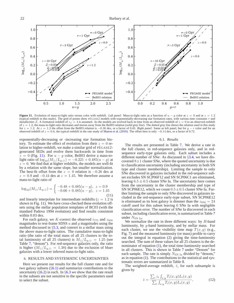
22 Barbary et al.

0.5 1.0 1.5 2.0 2.5ug

0.4

0.2

0.0

0.2

0.4

0.6

0.8

1.0

log10 (M

/Lg,

)

Z=0.01Z=0.02

z=0.0

Z=0.05

=0 Gyr=1 Gyr

=3 Gyr

=10 Gyrz=1.2

PEGASE model

Bell03 relation

0.0 0.2 0.4 0.6 0.8 1.0gr

0.4

0.2

0.0

0.2

0.4

0.6

0.8

1.0

log10 (M

/Lg,

)

Z=0.01Z=0.02

z=0.0

Z=0.05

=0 Gyr=1 Gyr

=3 Gyr

=10 Gyr

z=0.6

PEGASE model

Bell03 relation

Figure 11. Evolution of mass-to-light ratio versus color with redshift. Left panel: Mass-to-light ratio as a function ofu − g color atz = 0 and atz = 1.2(typical redshift in this study). The grid of points showPEGASE2 models with exponentially-decreasing star formation rates, with various time constantsτ andmetallicitiesZ. A formation redshift ofzf = 4 is assumed. As the models are evolved back in time from an observed redshift ofz = 0 to an observed redshiftof z = 1.2, the mass-to-light ratio decreases and moves away from the Bell03 relation (solid grey line). Thedotted grey lineshows the relation used in this studyfor z = 1.2. At z = 1.2 the offset from the Bell03 relation is−0.36 dex, or a factor of 0.43.Right panel:Same as left panel, but forg − r color and for anobserved redshift ofz = 0.6, the typical redshift in the rate study ofSharon et al.(2010). The offset here is only−0.14 dex, or a factor of 0.72.

exponentially-decreasing or -increasing star formation his-tory. To estimate the effect of evolution from theirz = 0 re-lation to higher-redshift, we make a similar grid ofPEGASE2-generated SEDs and evolve them backwards in time fromz = 0 (Fig. 11). For u − g color, Bell03 derive a mass-to-light ratio of log10(M⊙/Lg,⊙) = −0.221 + 0.485(u − g) atz = 0. We find that at higher redshifts, the models are well-fitby a relation with the same slope, but smaller normalization.The best-fit offset from thez = 0 relation is−0.26 dex atz = 0.9 and−0.44 dex atz = 1.45. We therefore assume amass-to-light ratio of

log10(M⊙/Lg,⊙) =

−0.48 + 0.485(u− g), z = 0.9−0.66 + 0.485(u− g), z = 1.45

(11)and linearly interpolate for intermediate redshifts (z = 1.2 isshown in Fig.11). We have cross-checked these evolution off-sets using the stellar population templates of BC03 (with thestandard Padova 1994 evolution) and find results consistentwithin 0.03 dex.

For each galaxy, weK-correct the observedi775 andz850magnitudes to rest-frame SDSSu andg magnitudes using themethod discussed in§5.3, and convert to a stellar mass usingthe above mass-to-light ratios. The cumulative mass-to-lightratio (the ratio of the total mass of all 25 clusters to the to-tal luminosity of all 25 clusters) isM⊙/Lg,⊙ = 1.25 (seeTable7, “denom”). For red-sequence galaxies only, the ratiois higher (M⊙/Lg,⊙ = 1.38) due to the exclusion of bluergalaxies with a lower inferred mass-to-light ratio.

6. RESULTS AND SYSTEMATIC UNCERTAINTIES

Here we present our results for the full cluster rate and fortwo galaxy subsets (§6.1) and summarize contributions to theuncertainty (§6.2) in each. In§6.3we show that the rate resultin the subsets are not sensitive to the specific parameters usedto select the subset.

6.1. Results

The results are presented in Table7. We derive a rate inthe full cluster, in red-sequence galaxies only, and in red-sequence early-type galaxies only. Each subset includes adifferent number of SNe: As discussed in§3.4, we have dis-covered8±1 cluster SNe, where the quoted uncertainty is dueto classification uncertainty (including uncertainty in both SNtype and cluster membership). Limiting the sample to onlySNe discovered in galaxies included in the red-sequence sub-set excludes SN SCP06F12 and SN SCP06C1 are eliminated,leaving6.5± 0.5 cluster SNe Ia. The uncertainty here comesfrom the uncertainty in the cluster membership and type ofSN SCP06E12, which we count0.5±0.5 cluster SNe Ia. Fur-ther limiting the sample to only SNe discovered in galaxies in-cluded in the red-sequence early-type subset, SN SCP06E12is eliminated as its host galaxy is dimmer than thez850 = 24cutoff used for this subset leaving6 SNe Ia with negligibleclassification error. The number of SNe Ia discovered in eachsubset, including classification error, is summarized in Table7underNSN Ia.

We normalize the rate in three different ways: byB-bandluminosity, byg-band luminosity, and by stellar mass. Foreach cluster, we use the visibility time mapT (x, y) (e.g.,Fig. 7) and the measured luminosity (or mass) profile to carryout the integral in equation (2) giving the time-luminositysearched. The sum of these values for all 25 clusters is the de-nominator of equation (1), the total time-luminosity searchedin all clusters. This is shown in Table7 under “Denom” foreach sample. The rate is simplyNSN Ia divided by “denom,”as in equation (1). The contributions to the statistical and sys-tematic errors are summarized in Table8.

The weighted-average redshift,z, for each subsample isgiven by

z =

∑

i zi∫

x,yTi(x, y)Li(x, y)

∑

i

∫

x,yTi(x, y)Li(x, y)

, (12)

The SN Ia Rate in High-Redshift Galaxy Clusters 23

Table 7Results

Environment Unit z NSN Ia Denom Rate (stat) (sys)

Full cluster SNuB 1.14 8.0± 1.0 15.87 0.50 +0.23−0.19

+0.10−0.09

Full cluster SNug · · · · · · 15.96 0.50 +0.23−0.19

+0.10−0.08

Full cluster SNuM · · · · · · 22.41 0.36 +0.16−0.13

+0.07−0.06

Red-sequence SNuB 1.136.5± 0.5 11.95 0.54 +0.25−0.19

+0.07−0.07

Red-sequence SNug · · · · · · 12.20 0.53 +0.24−0.19

+0.07−0.07

Red-sequence SNuM · · · · · · 17.61 0.37 +0.17−0.13

+0.05−0.05

Red-sequence early-type SNuB 1.106.0± 0.0 7.29 0.82 +0.39−0.30

+0.09−0.08

Red-sequence early-type SNug · · · · · · 7.59 0.79 +0.38−0.29

+0.09−0.08

Red-sequence early-type SNuM · · · · · · 11.77 0.51 +0.24−0.19

+0.06−0.05

Note. — “Denom” is the denominator of equation (1) and has units of1012L⊙,B years,1012L⊙,g years and1012M⊙ years for rate units of SNuB, SNugand SNuM respectively.

Table 8Sources of Uncertainty

Full Red- Red-sequencecluster sequence early-type

Source of error (%) (%) (%)

StatisticalPoisson +40

−32+45−35

+47−36

Luminosity (stat) ±12 ±6 ±6Luminosity (cosmic var.) ±16 ±4 ±3

Total statistical +45−38

+46−35

+48−37

SystematicSN type classification ±13 ±8 · · ·

Control time: varyingMB+8−6

+8−6

+8−6

Control time: dust distribution +10−2 · · · · · ·

Luminosity: MAG AUTO corr. ±7 ±7 ±7Luminosity:K-correction ±3 ±3 ±3Luminosity: Faint galaxy corr. +2

−4 · · · · · ·

Luminosity:r > 0.6(0.8) Mpc ±4 ±1 ±1

Total systematic +20−17

+14−12

+11−10

Total statistical + systematic +49−42

+48−37

+49−38

wherezi, Li andTi are the redshift, luminosity and effectivevisibility time of the i-th cluster, respectively. The weighted-average redshift is slightly smaller for the red-sequence andred-sequence early-type galaxy subsets. This is because inthehigher-redshift clusters, a smaller fraction of galaxies meetthe subset requirements (seez < 1.2 versusz > 1.2 averagecluster luminosity in Table6).

6.2. Summary of Systematic Uncertainties

Throughout the paper, we have highlighted and addressedpossible sources of systematic uncertainty. Here we summa-rize these sources. In Table8 we show the relative contri-bution of each to the total systematic error, and compare tosources of statistical error.

(1) SN type classification:The uncertainty in the numberof SNe observed in each galaxy subset was addressed in§6.1.The fractional error in the rate is simply the fractional error inthe number observed.

(2) Control time: VaryingMB : In our control time simula-tions, we assumed a distribution of SN Ia light curve shapesand absolute magnitudes. To first order, the impact of these

assumptions on the control time is captured by varying theassumed SN Ia absolute magnitude (§4.3). Variations of±0.2 mag resulted in a rate change of+8

−6%(3) Control time: dust distribution:In §4.3 we assessed

the impact of varying amounts of dust extinction on the con-trol time. Assuming an unrealistically large amount of dust-affected SNe decreased the control time by 9% (increasingthe SN rate by10%), while decreasing the amount of dust-affected SNe increased the control time by2% (decreasingthe SN rate by2%). We do not apply this systematic errorto the red-sequence or red-sequence early-type subsets, aswehave independent evidence that the amount of dust is limitedin these environments.

(4) MAG AUTO correction: In computing the totalz850luminosity of each galaxy, we made a correction to theMAG AUTO magnitude ranging from∼10% atz850 = 20to ∼30% atz850 = 25. Varying the range ofn used in thesimulation by±1 affects the correction by±7%.

(5)K-correction: In §5.3, we noted that the scatter of BC03templates about the best-fitK-correction is typically less than0.03 mag. We use this value as the systematic error on theK-correction.

(6) Faint galaxy correction:The average correctionC re-ported in Table5 is 1.054. VaryingM∗ by ± 0.5 magnitudesresults in an average correction of 1.032 and 1.092 for−0.5

and+0.5 magnitudes, respectively. Thus, we assign+2%−4%

asthe systematic error on the rate associated with this correction.This error is not applied to the red-sequence or red-sequenceearly type subsets as faint galaxy light is counted in these sub-sets.

(7) Luminosity at large radii:In §5.5we assumed a modelfor the cluster luminosity profile atr > 0.6 Mpc (0.8 Mpc forred-sequence and red-sequence early-type subsets). Varyingthe model luminosity by±20% resulted in a±4% changein the full cluster rate. The change is much smaller (±1%)for the red galaxy subsets because the model is only used atr > 0.8 Mpc.

6.3. Effect of Varying Subset Requirements

In selecting our red-sequence and red-sequence early-typegalaxy subsamples, we required red-sequence galaxies to bewithin ±0.2 mag of the color of their cluster red sequence.For early-type galaxies, we required the asymmetry parame-ter to be< 0.1 and the Gini coefficient to be> 0.40. It isinteresting to test the sensitivity of the results to variations in

24 Barbary et al.

0.05 0.10 0.15 0.20 0.25Red sequence half-width (mag)

0.0

0.2

0.4

0.6

0.8

1.0S

N I

a R

ate

(10

12M

1

yr

1)

Red-sequence SN Ia rate

Figure 12. The effect of varying the width of the red sequence. The nominalred-sequence rate result corresponds to a half-width of 0.20 mag. The innerand outer error bars represent the statistical and total uncertainty, respectively.

0.06 0.04 0.02 0.00 0.02 0.04 0.06 Gini, Asymmetry

0.0

0.2

0.4

0.6

0.8

1.0

SN

Ia R

ate

(10

12M

1

yr

1)

Red-sequence early-type SN Ia rate

Figure 13. The effect of varying the morphology parameter requirements.Negative∆ values correspond to a more strict selection and a higher-purityearly-type galaxy sample. The requirements are asymmetry< 0.1 + ∆ andGini coefficient> 0.40 − ∆. The nominal red-sequence early-type ratecorresponds to∆ = 0. The red-sequence half-width is fixed at 0.2 mag.The inner and outer error bars represent the statistical andtotal uncertainty,respectively.

the requirements. In Figures12 and13 we vary the require-ments and observe the effect on the rates. As requirements aremade more strict (for example, narrowing the red sequence)the total mass of the sample decreases. At the same time,SNe fall out of the sample when their host galaxies are cut.The Poisson error increases as the number of included SNeshrinks.

There is not a strong dependence of the SN Ia rate withgalaxy color residual from the red sequence (Fig.12). Evenin cluster galaxies that lie in a tight range around the red-sequence (±0.08 mag), we find a SN Ia rate consistent withthe full cluster rate. Similarly, there is no significant rate trendwith the purity of the early-type sample (Fig.13). We hap-pened to pick morphology requirements that yield a slightlyhigher rate than other choices, but such variations are ex-pected with small-number statistics and are accounted for bythe Poisson uncertainty in the result (Tables7 and8). Even inthe most-selective subset (∆ = −0.04), the rate is consistentwith the full cluster rate.

7. DISCUSSION AND CONCLUSIONS

7.1. Host-less Cluster SNe Ia

As reported by Dawson09, we have discovered one poten-tial host-less cluster SN Ia among the8 ± 1 cluster SNe Ia.SN SCP06C1 is projected near two possible host galaxies: Az850 = 21.6 spiral galaxy1′′.1 West of the SN, and a sig-nificantly fainterz850 = 24.6 galaxy0′′.45 (∼3.5 kpc at thecluster redshift) Northeast of the SN (See Dawson09, Fig. 2).

The galaxy-subtracted SN spectrum clearly shows a SN Iaat redshiftz = 0.98 near maximum light, consistent with thelight curve fit. The redshift ofz = 0.98 ± 0.01 is consistentwith the cluster redshift of 0.974. The bright spiral galaxyisactually in the background of the cluster, atz = 1.091. Strong[OII ] emission is visible in the spectrum, along with Ca H &K and Hδ absorption. Unfortunately, the small separation be-tween the main galaxy and the smaller galaxy to the Northeastmeans that the spectrum of the smaller galaxy is dominated bylight from the larger galaxy, making it impossible to assessaredshift. It is thus possible that the small galaxy is at the clus-ter redshift and is the actual host of the SN. Alternatively,thesmall galaxy might be at the same redshift as the larger galaxyand physically associated with it (either as a satellite galaxyor as part of the spiral structure of the galaxy).

We might hope to gain insight into the host from the SNparameters. We expect the intracluster medium to host an oldstellar component. SNe occurring in this population wouldhave parameters similar to those in passive elliptical galax-ies, namely a low stretch value. If the stretch were& 1.2,we might be able to conclude that the SN came from a youngpopulation (e.g.,Brandt et al. 2010). However, the stretch ofSN SCP06C1 is approximately 1.0 (Suzuki et al., in prepara-tion), which is on the high side of the distribution in passivegalaxies, but not unusual.

It is interesting to note that the SN is only20′′ (160 kpc)projected radius from the center of the cluster, perhaps giv-ing more weight to the hypothesis that it is associated with adiffuse intracluster stellar component.

Not being able to confirm or reject this SN as host-less,we have an upper limit of one host-less SN out of a total of8 ± 1. Discovering one host-less SNe Ia out of seven totalwould imply an intrinsic host-less SN Ia fraction of14%+18%

−7%

(binomial 68% confidence intervals), and a 95% upper limitof < 47%. These confidence intervals are similar to thoseof lower-redshift host-less SN Ia constraints (Gal-Yam et al.2003; Sharon et al. 2010) (although Gal-Yam et al. were ableto confirm the host-less nature of their SNe using deeperfollow-up imaging). The upper limit is consistent with di-rect measurements of intracluster light at low redshift, butdoes not strongly constrain evolution. A sample twice the sizeor larger, with deeper follow-up to confirm host-less SNe Iawould begin to place interesting constraints on hypothesesforthe formation of the intracluster stellar component fromz > 1to today.

7.2. Comparison to Other Cluster Rate Measurements

Cluster SN Ia rates have been reported at lower redshiftsby several groups. In nearby (z . 0.2) clusters, measure-ments include those ofSharon et al.(2007) at z ∼ 0.14,Mannucci et al.(2008) at z ∼ 0.02, andDilday et al.(2010)at z ∼ 0.09 and z ∼ 0.22. At intermediate redshifts,Sharon et al.(2010) recently reported the rate in0.5 <

The SN Ia Rate in High-Redshift Galaxy Clusters 25

z < 0.9 clusters (medianz ∼ 0.6). At higher redshifts,Gal-Yam et al.(2002) placed the first constraints on thez &0.8 cluster rate using a sample of three clusters atz = 0.83,0.89 andz = 1.27. However, their SN sample included onlyone firm SN Ia atz = 0.83. The resulting rate has corre-spondingly large uncertainties and essentially places only anupper limit on thez > 0.9 cluster rate. Our result is thus alarge step forward in the measurement of the SN rate in thehighest-redshift clusters.

In Figure 14 we compare our full cluster rate to thelower-redshift rate measurements that have been normalizedby stellar mass, permitting a comparison across redshifts.Here we have made an adjustment to the value reported bySharon et al.(2010). Sharon et al. used the mass-to-light ra-tio of Bell03 for the SDSSg andr bands, but did not applya correction for evolution betweenz ∼ 0.6 andz = 0. Us-ing the method described in§5.7 we find that a−0.14 dexoffset should be applied to the mass to account for evolutionfrom z = 0.6 to z = 0 (Fig. 11, right panel). We thereforeadjust the reported rate of Sharon et al. upward by 0.14 dex(38%). The rate compilation of Maoz10 reflects this adjust-ment. Whereas the adjusted Sharon et al. rate shows an in-dication that the cluster rate is increasing with redshift,forthe first time we find an increasing rate with high significance(> 2σ).

We point out that the popular “A + B” model(Scannapieco & Bildsten 2005) is insufficient for describingthe change in cluster rate with redshift. In this model theSN rate is the sum of a term proportional to the total stel-lar mass and a term proportional to the recent star formationrate:RSN Ia = AM∗ + BM∗. This simple model is conve-nient for predicting the SN rate in environments with vary-ing amounts of recent star formation as it accounts for theincreased SN Ia rate at short delay times. (In fact, we usethis model in Meyers10 to derive limits on the expected ratioof SNe Ia to SNe CC in early-type galaxies.) However, be-yond the fact that it matches predictions of an increased rateat short delay times, it is not theoretically motivated. In par-ticular, it is not detailed enough to describe the cluster rateobservations: In clusters, theA component is dominant at allredshifts observed. AsM∗ is not changing significantly withredshift, the rate would be expected to remain constant underthis model. To describe these observations, we require a DTDmodel wherein the rate decreases at large delay times (as itdoes in most theoretically-motivated models).

7.3. The Cluster SN Ia Delay Time Distribution

To illustrate the cluster rate constraints on the DTD, We pa-rameterize the late-time delay time distribution with a powerlaw in time,Ψ(t) ∝ ts. A power law is not only a conve-nient parameterization in the face of limited data, but is atheoretically-motivated function for the DD scenario, wherethe late-time (t & 1 Gyr) DTD shape is set by the distributionof WD separation after the second CE phase (Greggio 2005).

The cluster rates constrainΨ(t) from delay times of a fewGyr to∼ 10 Gyr. Here, we assume that the cluster ages corre-spond to the elapsed time since a formation redshift ofzf = 3(Fig. 14). This is consistent with measurements of clusterelliptical galaxies showing that star formation was mostlycompleted by this redshift (e.g.,Gobat et al. 2008). Our ratemeasurements in red and early-type galaxies provide a goodconsistency check that recent star formation does not signif-icantly contribute to the SN Ia rate: if it did, we would ob-

0.0 0.2 0.4 0.6 0.8 1.0 1.2 1.4z

10-1

100

SN

Ia R

ate

(10

12M

1

yr

1) t1.31

t1.71

t0.76

Sharon et al. (2010) 1.38Sharon et al. (2007)Mannucci et al. (2008)Dilday et al. (2010)This Work

2345678910

Time since zf =3 in Gyr

Figure 14. Cluster rate measurements (all galaxy types) from this work andthe literature. The rate ofSharon et al.(2010) shown has been adjusted up-ward by 38% from the reported rate (see text). The top axis shows the timeelapsed since an assumed cluster formation redshift ofzf = 3. The solidgrey linerepresents the best-fit power-law DTD (Ψ(t) ∝ ts), while thedot-ted grey linesshow the range of1σ error ons.

serve a higher rate in the full cluster than in these subsamples.Mannucci et al.(2008) find similar limits on the contributionto the cluster rate from late-type galaxies at low redshift.

With the inferred stellar ages, the cluster rate measure-ments can be interpreted as the DTD, after a correction: thecluster rate measurements are normalized bycurrent stellarmass whereas the DTD is normalized byinitial stellar mass.The DTD, Ψ(t) is therefore related to the cluster rate byΨ(t) = m(t)RSN Ia(t) wherem(t) is the fraction of stel-lar mass remaining at timet after the star formation burst.Stellar population synthesis models (e.g., BC03 orPEGASE2)show that over the age range of interest (∼3 to 11 Gyr) thestellar mass declines by about 10%. We follow Maoz10 in us-ing the stellar mass decline tabulated by BC03, but correctedby m(t) = 1 − 0.7mloss(t) to effectively convert from theSalpeter IMF used in BC03 to a “diet” Salpeter IMF. We finda best-fit value of

s = −1.31+0.55−0.40, (13)

and in Figure14, we plotRSN Ia(t) = Ψ(t)/m(t) for thisvalue. Theχ2 of the best-fit model is particularly small: 0.76for 4 degrees of freedom. (The probability of finding a smallerχ2 value is∼ 6%.) Varying our assumption ofzf = 3 doesnot have a significant impact on the results, given the mea-surement uncertainty. Withzf = 4, we finds = −1.43 andwith zf = 2.5, s = −1.21. (See Maoz10 for a detailed treat-ment of variations from the single-burst assumption.)

This result is consistent with measurements of the late-timeDTD in the field (Totani et al. 2008). It is also consistentwith the value ofs ∼ −1 typically predicted for the DDscenario (but note that this prediction can vary depending onthe distribution of WD separation). Most predictions for the

26 Barbary et al.

SD scenario show a steeper late-time DTD (Greggio 2005;Ruiter et al. 2009; Mennekens et al. 2010) with an effectivevalue fors ranging froms ∼ −1.3 (Greggio 2005) to s < −3(Mennekens et al. 2010). However, some groups have foundthat the SD scenario could be consistent withs ∼ −1 giventhe right combination of main sequence and red giant secon-daries (Hachisu et al. 2008).

7.4. Conclusions

In this paper, we have made a measurement of the high-redshift cluster SN Ia rate. Thanks to an unusually com-plete dataset (particularly for a rate study) the measurementis quite robust, with statistical and systematic uncertainties onpar with or better than measurement uncertainties at low red-shift. We highlight several important and/or unique aspects ofthe measurement:

• The SN classification approach takes advantage of allrelevant information. Thanks to the “rolling search”strategy of the survey and the nearly complete spec-troscopic follow-up, most candidates have a full lightcurve and a host galaxy redshift, greatly reducing clas-sification uncertainty.

• The position-dependent control time allows one to cal-culate a supernova rate given an arbitrary observing pat-tern and luminosity distribution.

• The control time calculation includes a full distributionof SN properties and the systematic uncertainty associ-ated with the assumed distribution is carefully quanti-fied. Thanks to the depth of the observations, the de-tection efficiency approaches 100% during the periodof the survey for most of the clusters, meaning that thesystematic uncertainty is low.

• Statistical uncertainties associated with the cluster lu-minosities, including both statistical variations and cos-mic variance, are included in the total uncertainty.Also, light in the outskirts of each galaxy (outside theSEXTRACTOR MAG AUTO aperture) is accounted for.This is a significant component of the total cluster lu-minosity.

• Cluster SN Ia rate measurements are normalized con-sistently across redshifts using a redshift-dependentmass-to-light versus color relation.

For the first time our result shows at the> 2σ level that thecluster SN Ia rate is increasing with redshift. Simply by com-paring the low- and high-redshift cluster rate measurements,the shape of the late-time SN Ia delay time distribution can beconstrained. The power of the measurement for this purposecomes both from the high redshift and relatively low statis-tical and systematic uncertainties in the measurement. Whilewe cannot conclusively rule out either the single degenerate ordouble degenerate class of progenitors via the delay time dis-tribution, the binary evolution that could lead to each modelare constrained. The DD scenario is consistent with the mea-surement under a wide range of plausible binary evolution pa-rameters, while there is a stronger constraint on binary scenar-ios that could lead to an SD scenario. Finally, this measure-ment is unique in constraining the delay time distribution atdelay times of a few Gyr. In future studies, it can be used incombination with other cluster rates and other delay time dis-tribution measurements (e.g., Maoz10) to place even tighter

constraints on models for binary evolution and SN Ia progen-itor scenarios.

We thank Eric Bell and Dan Maoz for helpful discussion.T. M. is financially supported by the Japan Society for thePromotion of Science (JSPS) through the JSPS Research Fel-lowship. C. L. is financially supported by the AustralianResearch Council (ARC) through the ARC Future Fellow-ship program. Financial support for this work was providedby NASA through program GO-10496 from the Space Tele-scope Science Institute, which is operated by AURA, Inc., un-der NASA contract NAS 5-26555. This work was also sup-ported in part by the Director, Office of Science, Office ofHigh Energy and Nuclear Physics, of the U.S. Department ofEnergy under Contract No. AC02-05CH11231, as well as aJSPS core-to-core program “International Research Networkfor Dark Energy” and by a JSPS research grant (20040003).The authors wish to recognize and acknowledge the very sig-nificant cultural role and reverence that the summit of MaunaKea has always had within the indigenous Hawaiian commu-nity. We are most fortunate to have the opportunity to conductobservations from this mountain. Finally, this work would nothave been possible without the dedicated efforts of the day-time and nighttime support staff at the Cerro Paranal Obser-vatory.

Facilities: HST (ACS), Subaru (FOCAS), Keck:I (LRIS),Keck:II (DEIMOS), VLT:Antu (FORS2)

REFERENCES

Amanullah, R., et al. 2010, ApJ, 716, 712Andreon, S. 2006a, in The Fabulous Destiny of Galaxies: Bridging Past and

Present, ed. V. Le Brun, A. Mazure, S. Arnouts, & D. Burgarella, 463Andreon, S. 2006b, MNRAS, 369, 969—. 2006c, A&A, 448, 447—. 2008, MNRAS, 386, 1045Andreon, S., de Propris, R., Puddu, E., Giordano, L., & Quintana, H. 2008a,

MNRAS, 383, 102Andreon, S., Puddu, E., de Propris, R., & Cuillandre, J. 2008b, MNRAS,

385, 979Andreon, S., Valtchanov, I., Jones, L. R., Altieri, B., Bremer, M., Willis, J.,

Pierre, M., & Quintana, H. 2005, MNRAS, 359, 1250Astier, P., et al. 2006, A&A, 447, 31Aubourg,E., Tojeiro, R., Jimenez, R., Heavens, A., Strauss, M. A., &

Spergel, D. N. 2008, A&A, 492, 631Barbary, K., et al. 2009, ApJ, 690, 1358Belczynski, K., Bulik, T., & Ruiter, A. J. 2005, ApJ, 629, 915Bell, E. F., McIntosh, D. H., Katz, N., & Weinberg, M. D. 2003,ApJS, 149,

289 (Bell03)Bertin, E. & Arnouts, S. 1996, A&AS, 117, 393Bohringer, H., Mullis, C., Rosati, P., Lamer, G., Fassbender, R., Schwope,

A., & Schuecker, P. 2005, The Messenger, 120, 33Brandt, T. D., Tojeiro, R., Aubourg,E., Heavens, A., Jimenez, R., & Strauss,

M. A. 2010, AJ, 140, 804Bremer, M. N., et al. 2006, MNRAS, 371, 1427Brodwin, M., et al. 2006, ApJ, 651, 791Bruzual, G. & Charlot, S. 2003, MNRAS, 344, 1000 (BC03)Butcher, H. & Oemler, Jr., A. 1978, ApJ, 219, 18—. 1984, ApJ, 285, 426Cain, B., et al. 2008, ApJ, 679, 293Calura, F., Matteucci, F., & Tozzi, P. 2007, MNRAS, 378, L11Cappellaro, E., Evans, R., & Turatto, M. 1999, A&A, 351, 459Cardelli, J. A., Clayton, G. C., & Mathis, J. S. 1989, ApJ, 345, 245Chatzopoulos, E., Wheeler, J. C., & Vinko, J. 2009, ApJ, 704, 1251Crawford, S. M., Bershady, M. A., & Hoessel, J. G. 2009, ApJ, 690, 1158Dawson, K. S., et al. 2009, AJ, 138, 1271 (Dawson09)Dilday, B., et al. 2010, ApJ, 713, 1026Eisenhardt, P. R. M., et al. 2008, ApJ, 684, 905Elston, R. J., et al. 2006, ApJ, 639, 816Feldmeier, J. J., Ciardullo, R., & Jacoby, G. H. 1998, ApJ, 503, 109Feldmeier, J. J., Ciardullo, R., Jacoby, G. H., & Durrell, P. R. 2004, ApJ,

615, 196Ferguson, H. C., Tanvir, N. R., & von Hippel, T. 1998, Nature,391, 461Fioc, M. & Rocca-Volmerange, B. 1997, A&A, 326, 950Fruchter, A. S. & Hook, R. N. 2002, PASP, 114, 144

The SN Ia Rate in High-Redshift Galaxy Clusters 27

Gal-Yam, A., Maoz, D., Guhathakurta, P., & Filippenko, A. V. 2003, AJ,125, 1087

Gal-Yam, A., Maoz, D., & Sharon, K. 2002, MNRAS, 332, 37Gansicke, B. T., Levan, A. J., Marsh, T. R., & Wheatley, P. J. 2009, ApJ,

697, L129Giavalisco, M., et al. 2004, ApJ, 600, L93Gilbank, D. G., Yee, H. K. C., Ellingson, E., Hicks, A. K., Gladders, M. D.,

Barrientos, L. F., & Keeney, B. 2008, ApJ, 677, L89Gobat, R., Rosati, P., Strazzullo, V., Rettura, A., Demarco,R., & Nonino, M.

2008, A&A, 488, 853Gonzalez, A. H., Zabludoff, A. I., & Zaritsky, D. 2005, ApJ, 618, 195Gonzalez, A. H., Zabludoff, A. I., Zaritsky, D., & Dalcanton, J. J. 2000,

ApJ, 536, 561Goto, T., et al. 2002, PASJ, 54, 515Goto, T., et al. 2005, ApJ, 621, 188Greggio, L. 2005, A&A, 441, 1055Greggio, L. & Renzini, A. 1983, A&A, 118, 217Guy, J., Astier, P., Nobili, S., Regnault, N., & Pain, R. 2005, A&A, 443, 781Hachisu, I., Kato, M., & Nomoto, K. 2008, ApJ, 683, L127Hakobyan, A. A., Petrosian, A. R., McLean, B., Kunth, D., Allen, R. J.,

Turatto, M., & Barbon, R. 2008, A&A, 488, 523Hamuy, M., Trager, S. C., Pinto, P. A., Phillips, M. M., Schommer, R. A.,

Ivanov, V., & Suntzeff, N. B. 2000, AJ, 120, 1479Hicken, M., Wood-Vasey, W. M., Blondin, S., Challis, P., Jha, S., Kelly,

P. L., Rest, A., & Kirshner, R. P. 2009, ApJ, 700, 1097Hicks, A. K., et al. 2008, ApJ, 680, 1022Hilton, M., et al. 2007, ApJ, 670, 1000Hsiao, E. Y., Conley, A., Howell, D. A., Sullivan, M., Pritchet, C. J.,

Carlberg, R. G., Nugent, P. E., & Phillips, M. M. 2007, ApJ, 663, 1187Iben, Jr., I. & Tutukov, A. V. 1984, ApJS, 54, 335Kessler, R., et al. 2009, ApJS, 185, 32Kobayashi, C. & Nomoto, K. 2009, ApJ, 707, 1466Koekemoer, A. M., Fruchter, A. S., Hook, R. N., & Hack, W. 2002,in The

2002 HST Calibration Workshop : Hubble after the Installation of theACS and the NICMOS Cooling System, ed. S. Arribas, A. Koekemoer, &B. Whitmore, 337

Kowalski, M., et al. 2008, ApJ, 686, 749Krick, J. E., Bernstein, R. A., & Pimbblet, K. A. 2006, AJ, 131,168Kuznetsova, N., et al. 2008, ApJ, 673, 981Kuznetsova, N. V. & Connolly, B. M. 2007, ApJ, 659, 530Li, W., et al. 2010, submitted (arXiv:1006.4612)Lin, Y.-T. & Mohr, J. J. 2004, ApJ, 617, 879Livio, M. 2001, in Supernovae and Gamma-Ray Bursts: the Greatest

Explosions since the Big Bang, ed. M. Livio, N. Panagia, & K. Sahu,334–355

Loewenstein, M. 2006, ApJ, 648, 230Mannucci, F., Della Valle, M., & Panagia, N. 2006, MNRAS, 370, 773Mannucci, F., Della Valle, M., Panagia, N., Cappellaro, E.,Cresci, G.,

Maiolino, R., Petrosian, A., & Turatto, M. 2005, A&A, 433, 807Mannucci, F., Maoz, D., Sharon, K., Botticella, M. T., DellaValle, M.,

Gal-Yam, A., & Panagia, N. 2008, MNRAS, 383, 1121Maoz, D. & Gal-Yam, A. 2004, MNRAS, 347, 951Maoz, D., Sharon, K., & Gal-Yam, A. 2010, ApJ, 722, 1879 (Maoz10)Matteucci, F. & Greggio, L. 1986, A&A, 154, 279Matteucci, F. & Recchi, S. 2001, ApJ, 558, 351Melbourne, J., et al. 2007, AJ, 133, 2709Mennekens, N., Vanbeveren, D., De Greve, J. P., & De Donder, E. 2010,

A&A, 515, A89Mihos, J. C., Harding, P., Feldmeier, J., & Morrison, H. 2005,ApJ, 631, L41Morokuma, T., et al. 2010, PASJ, 62, 19Mullis, C. R., Rosati, P., Lamer, G., Bohringer, H., Schwope, A., Schuecker,

P., & Fassbender, R. 2005, ApJ, 623, L85Nugent, P., Kim, A., & Perlmutter, S. 2002, PASP, 114, 803Peng, C. Y., Ho, L. C., Impey, C. D., & Rix, H. 2002, AJ, 124, 266Perlman, E. S., Horner, D. J., Jones, L. R., Scharf, C. A., Ebeling, H.,

Wegner, G., & Malkan, M. 2002, ApJS, 140, 265

Perlmutter, S., et al. 1999, ApJ, 517, 565Perlmutter, S., et al. 1997, ApJ, 483, 565Perlmutter, S., et al. 1995, ApJ, 440, L41Postman, M., Lubin, L. M., & Oke, J. B. 2001, AJ, 122, 1125Poznanski, D., Maoz, D., & Gal-Yam, A. 2007a, AJ, 134, 1285Poznanski, D., et al. 2007b, MNRAS, 382, 1169Pritchet, C. J., Howell, D. A., & Sullivan, M. 2008, ApJ, 683,L25Quimby, R. M., et al. 2009, preprint (arXiv:0910.0059)Richardson, D., Branch, D., Casebeer, D., Millard, J., Thomas, R. C., &

Baron, E. 2002, AJ, 123, 745Riess, A. G., et al. 1998, AJ, 116, 1009Rix, H., et al. 2004, ApJS, 152, 163Rosati, P., Stanford, S. A., Eisenhardt, P. R., Elston, R., Spinrad, H., Stern,

D., & Dey, A. 1999, AJ, 118, 76Rosati, P., et al. 2004, AJ, 127, 230Rosati, P., et al. 2009, A&A, 508, 583Ruiter, A. J., Belczynski, K., & Fryer, C. 2009, ApJ, 699, 2026Ruiz-Lapuente, P., Burkert, A., & Canal, R. 1995, ApJ, 447, L69Ruiz-Lapuente, P. & Canal, R. 1998, ApJ, 497, L57Sanchez-Blazquez, P., Gorgas, J., Cardiel, N., & Gonzalez, J. J. 2006, A&A,

457, 809Santos, J. S., et al. 2009, A&A, 501, 49Sarkar, D., Amblard, A., Cooray, A., & Holz, D. E. 2008, ApJ, 684, L13Scannapieco, C., Tissera, P. B., White, S. D. M., & Springel, V. 2006,

MNRAS, 371, 1125Scannapieco, E. & Bildsten, L. 2005, ApJ, 629, L85Schawinski, K. 2009, MNRAS, 397, 717Schechter, P. 1976, ApJ, 203, 297Sersic, J. L. 1968, Atlas de galaxias australes, ed. Sersic, J. L.Sharon, K., et al. 2010, ApJ, 718, 876Sharon, K., Gal-Yam, A., Maoz, D., Filippenko, A. V., & Guhathakurta, P.

2007, ApJ, 660, 1165Sivanandam, S., Zabludoff, A. I., Zaritsky, D., Gonzalez, A.H., & Kelson,

D. D. 2009, ApJ, 691, 1787Soker, N., Frankowski, A., & Kashi, A. 2010, New A, 15, 189Stanford, S. A., et al. 2005, ApJ, 634, L129Stanford, S. A., Eisenhardt, P. R., & Dickinson, M. 1998, ApJ, 492, 461Stanford, S. A., Holden, B., Rosati, P., Eisenhardt, P. R., Stern, D., Squires,

G., & Spinrad, H. 2002, AJ, 123, 619Stanford, S. A., et al. 2006, ApJ, 646, L13Strazzullo, V., et al. 2006, A&A, 450, 909Strolger, L.-G., et al. 2004, ApJ, 613, 200Sullivan, M., et al. 2006, ApJ, 648, 868Thielemann, F., Nomoto, K., & Hashimoto, M. 1996, ApJ, 460, 408Thomas, D., Maraston, C., Bender, R., & Mendes de Oliveira, C.2005, ApJ,

621, 673Tornambe, A. 1989, MNRAS, 239, 771Tornambe, A. & Matteucci, F. 1986, MNRAS, 223, 69Totani, T., Morokuma, T., Oda, T., Doi, M., & Yasuda, N. 2008, PASJ, 60,

1327Trenti, M. & Stiavelli, M. 2008, ApJ, 676, 767Tsujimoto, T., Nomoto, K., Yoshii, Y., Hashimoto, M., Yanagida, S., &

Thielemann, F. 1995, MNRAS, 277, 945Tutukov, A. V. & Yungelson, L. R. 1994, MNRAS, 268, 871van Dokkum, P. G., Franx, M., Kelson, D. D., & Illingworth, G. D. 2001,

ApJ, 553, L39Webbink, R. F. 1984, ApJ, 277, 355Whelan, J. & Iben, I. J. 1973, ApJ, 186, 1007Yungelson, L. R. 2005, in Astrophysics and Space Science Library, Vol. 332,

White dwarfs: cosmological and galactic probes, ed. E. M. Sion,S. Vennes, & H. L. Shipman, 163–173

Yungelson, L. R. & Livio, M. 2000, ApJ, 528, 108Zibetti, S., White, S. D. M., Schneider, D. P., & Brinkmann, J. 2005,

MNRAS, 358, 949