Spectral estimates on the sphere

SPECTRAL ESTIMATES ON THE SPHERE

JEAN DOLBEAULT, MARIA J. ESTEBAN, AND ARI LAPTEV

Abstract. In this article we establish optimal estimates for the first eigenvalue of Schrodinger operatorson the d-dimensional unit sphere. These estimates depend on Lp norms of the potential, or of its inverse,

and are equivalent to interpolation inequalities on the sphere. We also characterize a semi-classical

asymptotic regime and discuss how our estimates on the sphere differ from those on the Euclidean space.

1. Introduction

Let ∆ be the Laplace-Beltrami operator on the unit d-dimensional sphere Sd. Our first result isconcerned with the sharp estimate of the first negative eigenvalue λ1 = λ1(−∆ − V ) of the Schrodingeroperator −∆− V on Sd (with potential −V ) in terms of Lp-norms of V .

The literature on spectral estimates for the negative eigenvalues of Schrodinger operators on manifoldsis limited. We can quote two papers of P. Federbusch and O.S. Rothaus, [16, 33], which establish alink between logarithmic Sobolev inequalities and the ground state energy of Schrodinger operators. TheRozenbljum-Lieb-Cwikel inequality (case γ = 0 with standard notations: see below) on manifolds has beenstudied in [25, Section 5]; we may also refer to [26] for the semi-classical regime, and to [24, 31] for morerecent results in this direction. In two articles (see [20, 21]) on Lieb-Thirring type inequalities (also see[24, 31] for other results on manifolds), A. Ilyin considers Schrodinger operators on unit spheres restrictedto the space of functions orthogonal to constants and uses the original method of E. Lieb and W. Thirringin [27]. The exclusion of the zero mode of the Laplace-Beltrami operator results in semi-classical estimatessimilar to those for negative eigenvalues of Schrodinger operators in Euclidean spaces.

The results in this paper are somewhat complementary. We show that if the Lp-norm of V is smallerthan an explicit value, then the first eigenvalue λ1(−∆−V ) cannot satisfy the semi-classical inequality andthus it is impossible to obtain standard Lieb-Thirring type inequalities for the whole negative spectrum.However, we show that if the Lp-norm of the potential is large then the first eigenvalue behaves semi-classically and the best constant in the inequality asymptotically coincides with the best constants L1

γ,d

of the corresponding inequality in the Euclidean space of same dimension (see below). In this regime thefirst eigenfunction is concentrated around some point on Sd and can be identified with an eigenfunctionof the Schrodinger operator on the tangent space, up to a small error. In Appendix A, we illustrate thetransition between the small Lp-norm regime and the asymptotic, semi-classical regime by numericallycomputing the optimal estimates for the eigenvalue λ1(−∆− V ) in terms of the norms ‖V ‖Lp(Sd).

In order to formulate our first theorem let us introduce the measure dω induced by Lebesgue’s measureon Sd ⊂ Rd+1 and the uniform probability measure dσ = dω/|Sd| with |Sd| = ω(Sd). We shall denote by‖·‖Lq(Sd) the quantity ‖u‖Lq(Sd) =

( ∫Sd |u|q dσ

)1/q for any q > 0 (hence including in the case q ∈ (0, 1),

for which ‖·‖Lq(Sd) is not anymore a norm, but only a quasi-norm). Because of the normalization of dσ,when making comparisons with corresponding results in the Euclidean space, we will need the constant

κq,d := |Sd|1− 2q .

The well-known optimal constant L1γ,d in the one bound state Keller-Lieb-Thirring inequality is defined as

follows: for any function φ on Rd, if λ1(−∆−φ) denotes the lowest negative eigenvalue of the Schrodinger

Date: December 12, 2013.Key words and phrases. Spectral problems; Partial differential operators on manifolds; Quantum theory; Estimation

of eigenvalues; Sobolev inequality; interpolation; Gagliardo-Nirenberg-Sobolev inequalities; logarithmic Sobolev inequality;Schrodinger operator; ground state; one bound state Keller-Lieb-Thirring inequality

Mathematics Subject Classification (2010). Primary: 58J50; 81Q10; 81Q35; 35P15. Secondary: 47A75; 26D10; 46E35;

58E35; 81Q20.

arX

iv:1

301.

1210

v2 [

mat

h.A

P] 1

6 Ju

n 20

13

2 J. DOLBEAULT , M.J. ESTEBAN, A. LAPTEV

operator −∆− φ (with potential −φ) when it exists, and 0 otherwise, we have

(1) |λ1(−∆− φ)|γ ≤ L1γ,d

∫Rdφγ+ d

2+ dx ,

provided γ ≥ 0 if d ≥ 3, γ > 0 if d = 2, and γ ≥ 1/2 if d = 1. Notice that only the positive part φ+ of φ isinvolved in the right-hand side of the above inequality. Assuming that γ > 1− d/2 if d = 1 or 2, we shallconsider the exponents

q = 22 γ + d

2 γ + d− 2and p =

q

q − 2= γ +

d

2,

which are therefore such that 2 < q = 2 pp−1 ≤ 2∗ with 2∗ := 2 d

d−2 if d ≥ 3, and q = 2 pp−1 ∈ (2,+∞) if

d = 1 or 2. To simplify notations, we adopt the convention 2∗ :=∞ if d = 1 or 2. It is also convenient tointroduce the notation

α∗ :=1

4d (d− 2) .

In Section 2 we shall prove the following result.

Theorem 1. Let d ≥ 1, p ∈(

max{1, d/2},+∞). Then there exists a convex increasing function α :

R+ → R+ with α(µ) = µ for any µ ∈[0, d2 (p− 1)

]and α(µ) > µ for any µ ∈

(d2 (p− 1),+∞

), such that

(2) |λ1(−∆− V )| ≤ α(‖V ‖Lp(Sd)

)for any nonnegative V ∈ Lp(Sd). Moreover, for large values of µ, we have

α(µ)p−d2 = L1

p− d2 ,d(κq,d µ)p (1 + o(1)) .

The estimate (2) is optimal in the sense that there exists a nonnegative function V such that µ = ‖V ‖Lp(Sd)

and |λ1(−∆ − V )| = α(µ) for any µ ∈(d2 (p − 1),+∞

). If µ ≤ d

2 (p − 1), equality in (2) is achieved byconstant potentials.

If p = d/2 and d ≥ 3, then (2) is satisfied with α(µ) = µ only for µ ∈ [0, α∗]. If d = p = 1, then (2)is also satisfied for some nonnegative, convex function α on R+ such that µ ≤ α(µ) ≤ µ + π2 µ2 for anyµ ∈ (0,+∞), equality in (2) is achieved and α(µ) = π2 µ2(1 + o(1)) as µ→ +∞.

Since λ1(−∆− V ) is nonpositive for any nonnegative, nontrivial V , inequality (2) is a lower estimate.We have indeed found that

0 ≥ λ1(−∆− V ) ≥ −α(‖V ‖Lp(Sd)

).

If V changes sign, the above inequality still holds if V is replaced by the positive part V+ of V , providedthe lowest eigenvalue is negative. We can then write

(3) |λ1(−∆− V )| ≤ α(‖V+‖Lp(Sd)

)∀V ∈ Lp(Sd) .

The expression of L1γ,d is not explicit (except in the case d = 1: see [27, p. 290]) but can be given in terms

of an optimal constant in some Gagliardo-Nirenberg-Sobolev inequality (see [27], and (9)–(10) below inSection 2.1). In case d = p = 1, notice that L1

1/2,1 = 1/2 (see Appendix B.2) and κ∞,1 = 2π so that our

formula in the asymptotic regime µ→ +∞ is consistent with the other cases.

The reader is invited to check that Theorem 1 can be reformulated in a more standard language ofspectral theory as follows. We recall that γ = p − d/2 and that dω is the standard measure induced onthe unit sphere Sd by Lebesgue’s measure on Rd+1.

Corollary 2. Let d ≥ 1 and consider a nonnegative function V . For µ = ‖V ‖Lγ+

d2 (Sd)

large, we have

(4) |λ1(−∆− V )|γ . L1γ,d

∫SdV γ+ d

2 dω

if either γ > max{0, 1 − d/2} or γ = 1/2 and d = 1. However, if µ = ‖V ‖Lγ+

d2 (Sd)

≤ 14 d (2 γ + d − 2),

then we have

(5) |λ1(−∆− V )|γ+ d2 ≤

∫SdV γ+ d

2 dω

for any γ ≥ max{0, 1− d/2} and this estimate is optimal.

SPECTRAL ESTIMATES ON THE SPHERE 3

Here the notation f . g as µ → +∞ means that f ≤ c(µ) g with limµ→∞ c(µ) = 1. The limit caseγ = max{0, 1 − d/2} in (5) is covered by approximations. We may also notice that optimality in (5) isachieved by constant potentials. Let us give some details.

If we consider a sequence of constant functions (Vn)n∈N uniformly converging towards 0, for instanceVn = 1/n, then we get that

limn→∞

|λ1(−∆− Vn)|γ∫Sd V

γ+ d2

n dω= +∞

which clearly forbids the possibility of an inequality of the same type as (4) for small values of∫Sd V

γ+ d2 dω.

This is however compatible with the results of A. Ilyin in dimension d = 2. In [21, Theorem 2.1], theauthor states that if P is the orthogonal projection defined by P u := u −

∫S2 u dω, then the negative

eigenvalues λk(P (−∆− V )P ) satisfy the semi-classical inequality∑k

|λk(P (−∆− V )P )| ≤ 3

8

∫S2V 2 dω .

Another way of seeing that inequalities like (4) are incompatible with small potentials is based on thefollowing observation. Inequality (5) shows that

|λ1(−∆− V )| ≤(∫

S2V 2 dω

)1/2

if the L2-norm of V is smaller than 1. Since such an inequality is sharp, the semi-classical Lieb-Thirringinequalities for the Schrodinger operator on the sphere S2 are therefore impossible for small potentials andcan be achieved only in a semi-classical asymptotic regime, that is, when the norm ‖V ‖L2(S2) is large.

Our second main result is concerned with the estimates from below for the first eigenvalue of Schrodingeroperators with positive potentials. In this case, by analogy with (1), it is convenient to introduce theconstant L1

−γ,d with γ > d/2 which is the optimal constant in the inequality:

(6) λ1(−∆ + φ)−γ ≤ L1−γ,d

∫Rdφd2−γ dx ,

where φ is any positive potential on Rd and λ1(−∆ +φ) denotes the lowest positive eigenvalue if it exists,or +∞ otherwise. Inequality (6) is less standard than (1): we refer to [15, Theorem 12] for a statementand a proof. As in Theorem 1, we shall also introduce exponents p and q such that

q = 22 γ − d

2 γ − d+ 2and p =

q

2− q = γ − d

2,

so that p (resp. q = 2 pp+1 ) takes arbitrary values in (0,+∞) (resp. (0, 2)). With these notations, we have

the counterpart of Theorem 1 in the case of positive potentials.

Theorem 3. Let d ≥ 1, p ∈ (0,+∞). There exists a concave increasing function ν : R+ → R+ withν(β) = β for any β ∈

[0, d2 (p + 1)

]if p > 1, ν(β) ≤ β for any β > 0 and ν(β) < β for any β ∈(

d2 (p+ 1),+∞

), such that

(7) λ1(−∆ +W ) ≥ ν(β)

with β = ‖W−1‖−1Lp(Sd)

,

for any positive potential W such that W−1 ∈ Lp(Sd). Moreover, for large values of β, we have

ν(β)− (p+ d2 ) . L1

−(p+ d2 ),d

(κq,d β)−p

.

The estimate (7) is optimal in the sense that there exists a nonnegative potential W such that β−1 =‖W−1‖Lp(Sd) and λ1(−∆+W ) = ν(β) for any positive β and p. If β ≤ d

2 (p+1) and p > 1, equality in (7)is achieved by constant potentials.

Again the expression of L1−γ,d is not explicit when d ≥ 2 but can be given in terms of an optimal

constant in some Gagliardo-Nirenberg-Sobolev inequality (see [15], and (17)–(18) below in Section 4).

We can rewrite Theorem 3 in terms of γ = p+ d/2 and explicit integrals involving W .


Corollary 4. Let d ≥ 1 and γ > d/2. For β = ‖W−1‖−1

Lγ−d2 (Sd)

large, we have

(λ1(−∆ +W )

)−γ. L1

−γ,d

∫SdW

d2−γ dω .

However, if γ ≥ d2 + 1 and if β = ‖W−1‖−1

Lγ−d2 (Sd)

≤ 14 d (2 γ − d+ 2), then we have

(λ1(−∆ +W )

) d2−γ ≤

∫SdW

d2−γ dω ,

and this estimate is optimal.

This paper is organized as follows. Section 2 contains various results on interpolation inequalities; themost important one for our purpose is stated in Lemma 5. Theorem 1, Corollary 2 and various spectralestimates for Schrodinger operators with negative potentials are established in Section 3. Section 4 dealswith the case of positive potentials and contains the proofs of Theorem 3 and Corollary 4. Section 5 isdevoted to the threshold case (q = 2, that is, p, γ → +∞) of exponential estimates for eigenvalues or, interms of interpolation inequalities, to logarithmic Sobolev inequalities. Finally numerical and technicalresults have been collected in two appendices.

2. Interpolation inequalities and consequences for negative potentials

2.1. Inequalities in the Euclidean space. Let us start by some considerations on inequalities in theEuclidean space, which play a crucial role in the semi-classical regime.

We recall that we denote by 2∗ the Sobolev critical exponent 2dd−2 if d ≥ 3 and consider Sobolev’s

inequality on Rd, d ≥ 3,

(8) ‖v‖2L2∗ (Rd) ≤ Sd ‖∇v‖2L2(Rd) ∀ v ∈ D1,2(Rd)

where Sd is the optimal constant and D1,2(Rd) is the Beppo-Levi space obtained by completion of smoothcompacty supported functions with respect to the norm v 7→ ‖∇v‖L2(Rd). See Appendix B.4 for detailsand comments on the expression of Sd.

Assume now that d ≥ 1 and recall that 2∗ = +∞ if d = 1 or 2. In the subcritical case, that is,q ∈ (2, 2∗), let

Kq,d := infv∈H1(Rd)\{0}

‖∇v‖2L2(Rd) + ‖v‖2L2(Rd)

‖v‖2Lq(Rd)

be the optimal constant in the Gagliardo-Nirenberg-Sobolev inequality

(9) Kq,d ‖v‖2Lq(Rd) ≤ ‖∇v‖2L2(Rd) + ‖v‖2L2(Rd) ∀ v ∈ H1(Rd) .

The optimal constant L1γ,d in the one bound state Keller-Lieb-Thirring inequality is such that

(10) L1γ,d := (Kq,d)

− pwith p = γ +

d

2, q = 2

2 γ + d

2 γ + d− 2.

See Appendix B.5 for a proof and references, and [27] for a detailed discussion. Also see [27, Appendix A.Numerical studies, by J.F. Barnes] for numerical values of Kq,d.

We shall also define the exponent

ϑ := dq − 2

2 q

which plays an important role in the scale invariant form of the Gagliardo-Nirenberg-Sobolev interpolationinequalities associated to Kq,d: see Appendix B.1 for details.


2.2. Interpolation inequalities on the sphere. Using the inverse stereographic projection (see Ap-pendix B.3), it is possible to relate interpolation inequalities on Rd with interpolation inequalities on Sd.In this section we consider the case of the sphere. Notice that α∗ = d/(q − 2) when q = 2∗ = 2 d/(d− 2),d ≥ 3.

Lemma 5. Let q ∈ (2, 2∗). Then there exists a concave increasing function µ : R+ → R+ with thefollowing properties

µ(α) = α ∀α ∈[0, d

q−2

]and µ(α) < α ∀α ∈

(dq−2 ,+∞

),

µ(α) =Kq,dκq,d

α1−ϑ (1 + o(1)) as α→ +∞ ,

such that

(11) ‖∇u‖2L2(Sd) + α ‖u‖2L2(Sd) ≥ µ(α) ‖u‖2Lq(Sd) ∀u ∈ H1(Sd) .

If d ≥ 3 and q = 2∗, the inequality also holds for any α > 0 with µ(α) = min {α, α∗}.

The remainder of this section is mostly devoted to the proof of Lemma 5. A fundamental tool is arigidity result proved by M.-F. Bidaut-Veron and L. Veron in [9, Theorem 6.1] for q > 2, which goes asfollows. Any positive solution of

(12) − ∆f + α f = fq−1

has a unique solution f ≡ α1/(q−2) for any 0 < α ≤ d/(q − 2). A straightforward consequence of thisrigidity result is the following interpolation inequality (see [9, Corollary 6.2]):

(13)

∫Sd|∇u|2 dσ ≥ d

q − 2

[(∫Sd|u|q dσ

)2/q

−∫Sd|u|2 dσ

]∀u ∈ H1(Sd, dσ) .

Inequality (13) holds for any q ∈ [1, 2) ∪ (2, 2∗] if d ≥ 3 and for any q ∈ [1, 2) ∪ (2,∞) if d = 1 or 2. Analternative proof of (13) has been established in [5] for q > 2 using previous results by E. Lieb in [28] andthe Funk-Hecke formula (see [17, 19]). The whole range p ∈ [1, 2) ∪ (2, 2∗) was covered in the case of theultraspherical operator in [7, 8]. Also see [4, 23] for the carre du champ method, and [14] for an elementaryproof. Inequality (13) is tight as defined by D. Bakry in [3, Section 2], in the sense that equality is achievedonly by constants.

Remark 6. Inequality (13) is equivalent to

infu∈H1(Sd)\{0}

(q − 2) ‖∇u‖2L2(Sd)

‖u‖2Lq(Sd)

− ‖u‖2L2(Sd)

= d .

Although we will not make use of them in this paper, we may notice that the following properties hold true:

(i) If q < 2∗, the above infimum is not achieved in H1(Sd) \ {0} but

limε→0+

(q − 2) ‖∇uε‖2L2(Sd)

‖uε‖2Lq(Sd)− ‖uε‖2L2(Sd)

= d

if uε := 1 + εϕ, where ϕ is a non-trivial eigenfunction of the Laplace-Beltrami operator corre-sponding the first nonzero eigenvalue (see below Section 2.3).

(ii) If q = 2∗, d ≥ 3, there are non-trivial optimal functions for (13), due to the conformal invariance.Alternatively, these solutions can be constructed from the family of Aubin-Talenti optimal functionsfor Sobolev’s inequality, using the inverse stereographic projection.

(iii) If α > α∗ and q = 2∗, d ≥ 3, there are no optimal functions for (11), since otherwise α 7→ µ(α)would not be constant on (α∗, α): see Proposition 7 below.


2.3. Properties of the function α 7→ µ(α) in the subcritical case. Assume that q ∈ (2, 2∗). For anyα > 0, consider

Qα[u] :=‖∇u‖2L2(Sd) + α ‖u‖2L2(Sd)

‖u‖2Lq(Sd)

∀u ∈ H1(Sd, dσ) .

It is a standard result of the calculus of variations that

infu ∈ H1(Sd, dσ)∫Sd |u|q dσ = 1

Qα[u] := µ(α)

is achieved by a minimizer u ∈ H1(Sd, dσ) which solves the Euler-Lagrange equations

(14) − ∆u+ αu− µ(α)uq−1 = 0 .

Indeed we know that there is a Lagrange multiplier associated to the constraint∫Sd |u|q dσ = 1, and

multiplying (14) by u and integrating on Sd, we can identify it with µ(α). As a corollary, we have shownthat (11) holds. The fact that the Lagrange multiplier can be identified so easily is a consequence of thefact that all terms in (11) are two-homogeneous.

We can now list some basic properties of the function α 7→ µ(α).

(1) For any α > 0, µ(α) is positive, since the infimum is achieved by a nonnegative function u andu = 0 is incompatible with the constraint

∫Sd |u|q dσ = 1. By taking a constant test function, we

see that µ(α) ≤ α, for all α > 0. The function α 7→ µ(α) is monotone nondecreasing since for agiven u ∈ H1(Sd, dσ) \ {0}, the function α 7→ Qα[u] is monotone increasing. It is actually strictlymonotone. Indeed if µ(α1) = µ(α2) with α1 < α2, then one can notice that Qα1

[u2] < µ(α1)if u2 is a minimizer of Qα2 satisfying the constraint

∫Sd |u2|q dσ = 1, which provides an obvious

contradiction.(2) We have

µ(α) = α ∀α ∈(

0, dq−2

].

Indeed, if u is a solution of (14), then f = µ(α)1/(q−2) u solves (12) and is therefore a constantfunction if α ≤ d/(q − 2) according to [9, Theorem 6.1], and so is u as well. Because of thenormalization constraint ‖u‖Lq(Sd) = 1, we get that u = 1, which proves the statement.

On the contrary, we have

µ(α) < α ∀α > d

q − 2.

Let us prove this. Let ϕ be a non-trivial eigenfunction of the Laplace-Beltrami operator corre-sponding the first nonzero eigenvalue:

−∆ϕ = dϕ .

If x = (x1, x2, ...xd, z) are cartesian coordinates of x ∈ Rd+1 so that Sd ⊂ Rd+1 is characterized

by the condition∑di=1 x

2i + z2 = 1, then a simple choice of such a function ϕ is ϕ(x) = z. By

orthogonality with respect to the constants, we know that∫Sd ϕ dσ = 0. We may now Taylor

expand Qα around u = 1 by considering u = 1 + εϕ as ε→ 0 and obtain that

µ(α) ≤ Qα[1 + εϕ] =(d+ α) ε2

∫Sd |ϕ|2 dσ + α(∫

Sd |1 + εϕ|q dσ)2/q = α+

[d+ α (2− q)

]ε2

∫Sd|ϕ|2 dσ + o(ε2) .

By taking ε small enough, we get µ(α) < α for all α > d/(q−2). Optimizing on the value of ε > 0(not necessarily small) provides an interesting test function: see Section A.1.

(3) The function α 7→ µ(α) is concave, because it is the minimum of a family of affine functions.


2.4. More estimates on the function α 7→ µ(α). We first consider the critical case q = 2∗, d ≥ 3.As in the subcritical case q < 2∗, we have µ(α) = α for α ≤ α∗. For α > α∗, the function α 7→ µ(α) isconstant:

Proposition 7. With the notations of Lemma 5, if d ≥ 3 and q = 2∗, then

µ(α) = α∗ ∀α > α∗ =d

q − 2=

1

4d (d− 2) .

Proof. Consider the Aubin-Talenti optimal functions for Sobolev’s inequality and more specifically, let uschoose the functions

vε(x) :=(

εε2+|x|2

) d−22 ∀x ∈ Rd , ∀ ε > 0 ,

which are such that ‖vε‖L2∗ (Rd) = ‖v1‖L2∗ (Rd) is independent of ε. With standard notations (see Appen-

dix B.3), let N ∈ Sd be the North Pole. Using the stereographic projection Σ, i.e. for the functions definedfor any y ∈ Sd \ {N} by

uε(y) =(|x|2+1

2

) d−22

vε(x) with x = Σ(y) ,

we find that ‖uε‖L2∗ (Sd) = ‖v1‖L2∗ (Rd) for any ε > 0, so that

µ(α) ≤ Qα[uε] =‖∇vε‖2L2(Rd) + (α− α∗)

∫Rd |vε|2

(2

1+|x|2)2dx

κ2∗,d ‖vε‖2L2∗ (Rd)

= α∗ + 4 |Sd|1− 2d (α− α∗)

δ(d, ε)

‖v1‖2L2∗ (Rd)

where we have used the fact that κ2∗,d Sd = 1/α∗ (see Appendix B.4) and

δ(d, ε) :=

∫ ∞0

(ε

ε2 + r2

)d−2rd−1

(1 + r2)2dr = ε2

∫ ∞0

(1

1 + s2

)d−2sd−1

(1 + ε2 s2)2ds .

One can check that limε→0+δ(d, ε) = 0 since

δ(d, ε) ≤ ε2

∫ ∞0

sd−1

(1 + s2)d−2ds if d ≥ 5 and δ(d, ε) ≤ ε cd

∫ +∞

0

ds

(1 + s2)2if d = 3 or 4 ,

with c3 = 1 and c4 = 3√

3/16. �

The next step is devoted to a lower estimate for the function α 7→ µ(α) in the subcritical case, whichshows that limα→+∞ µ(α) = +∞ in contrast with the critical case.

Proposition 8. With the notations of Lemma 5, if d ≥ 3 and q ∈ (2, 2∗), then for any α > α∗ we have

α > µ(α) ≥ αϑ∗ α1−ϑ ,

with ϑ = d q−22 q . For every s ∈ (2, 2∗) if d ≥ 3, or every s ∈ (2,+∞) if d = 1 or 2, such that s > q, we

also have that

α > µ(α) ≥(

ds−2

)θα1−θ ,

for any α > d/(s− 2) and θ = θ(s, q, d) := s (q−2)q (s−2) .

Proof. The first case can be seen as a limit case of the second one as s → 2∗ and ϑ = θ(2∗, q, d). UsingHolder’s inequality, we can estimate ‖u‖Lq(Sd) by

‖u‖Lq(Sd) ≤ ‖u‖θLs(Sd) ‖u‖1−θL2(Sd)

and get the result using

Qα[u] ≥(‖∇u‖2L2(Sd) + α ‖u‖2L2(Sd)

‖u‖2Ls(Sd)

)θ (‖∇u‖2L2(Sd) + α ‖u‖2L2(Sd)

‖u‖2L2(Sd)

)1−θ

≥(

ds−2

)θα1−θ .

�

Proposition 9. With the notations of Lemma 5, for every q ∈ (2, 2∗) we have

lim supα→+∞

αϑ−1µ(α) ≤ Kq,dκq,d

.


Proof. Let v be an optimal function for Kq,d and define for any x ∈ Rd the function

vα(x) := v(2√α− α∗ x

)with α∗ = 1

4 d (d− 2) and α > α∗, so that∫Rd|∇vα|2 dx = 22−d (α− α∗)1− d2

∫Rd|∇v|2 dx ,

∫Rd|vα|q

(2

1+|x|2)d−(d−2) q2

dx = 2−(d−2) q2 (α− α∗)−d2

∫Rd|v|q

(1 + |x|2

4 (α−α∗))−d+(d−2) q2 dx .

Now we observe that the function uα(y) :=( |x|2+1

2

)(d−2)/2vα(x), where y = Σ−1(x) and Σ is the stereo-

graphic projection (see Appendix B.3), is such that

Qα[uα] =1

κq,d

∫Rd |∇vα|2 dx+ (α− α∗)

∫Rd |vα|2

(2

1+|x|2)2

dx[ ∫Rd |vα|q

(2

1+|x|2)d−(d−2) q2

dx] 2q

.

Passing to the limit as α→ +∞, we get

limα→+∞

∫Rd|v|q

(1 + |x|2

4 (α−α∗))−d+(d−2) q2 dx =

∫Rd|v|q dx

by Lebesgue’s theorem of dominated convergence. The limit also holds with q replaced by 2. This provesthat

Qα[uα] = (α− α∗)1− d2 + dq

(Kq,dκq,d

+ o(1)

)as α→ +∞

which concludes the proof because ϑ = d (q − 2)/(2 q). �

2.5. The semi-classical regime: behavior of the function α 7→ µ(α) as α → +∞. Assume thatq ∈ (2, 2∗). If we combine the results of Propositions 8 and 9, we know that µ(α) ∼ α1−ϑ as α → +∞ ifd ≥ 3. If d = 1 or 2, we know that limα→+∞ µ(α) = +∞ with a growth at least equivalent to α2/q−ε withε > 0, arbitrarily small, according to Proposition 8, and at most equivalent to α1−ϑ by Proposition 9. Tocomplete the proof of Lemma 5, it remains to determine the precise behavior of µ(α) as α→ +∞.

Proposition 10. With the notations of Lemma 5, for every q ∈ (2, 2∗), with ϑ = d q−22 q we have

µ(α) =Kq,dκq,d

α1−ϑ(1 + o(1)) as α→ +∞ .

Proof. Suppose by contradiction that there is a positive constant η and a sequence (αn)n∈N such thatlimn→+∞ αn = +∞ and

(15) limn→+∞

αϑ−1n µ(αn) ≤ Kq,d

κq,d− η .

Consider a sequence (un)n∈N of functions in H1(Sd) such that Qαn [un] = µ(αn) and ‖un‖Lq(Sd) = 1 forany n ∈ N. From (15), we know that

αn ‖un‖2L2(Sd) ≤ Qαn [un] = µ(αn) ≤ α1−ϑn

(Kq,dκq,d

− η)

(1 + o(1)) as n→ +∞

that is

lim supn→+∞

αϑn ‖un‖2L2(Sd) ≤Kq,dκq,d

− η .

The normalization ‖un‖Lq(Sd) = 1 for any n ∈ N and the limit limn→+∞ ‖un‖L2(Sd) = 0 mean that the

sequence (un)n∈N concentrates: there exists a sequence (yi)i∈N of points in Sd (eventually finite) andtwo sequences of positive numbers (ζi)i∈N and (ri,n)i,n∈N such that limn→+∞ ri,n = 0, Σi∈Nζi = 1 and∫Sd∩B(yi,ri,n)

|ui,n|q dσ = ζi + o(1), where ui,n ∈ H1(Sd), ui,n = un on Sd ∩ B(yi, ri,n) and supp ui,n ⊂Sd∩B(yi, 2 ri,n). Here o(1) means that uniformly with respect to i, the remainder term converges towards


0 as n→ +∞. A computation similar to those of the proof of Proposition 9, we can blow up each functionui,n and prove

(αn − α∗)ϑ−1

∫Sd

(|∇ui,n|2 + αn |ui,n|2

)dσ ≥ Kq,d

κq,dζ

2/qi + o(1) ∀ i .

Let us choose an integer N such that(ΣNi=1ζi

)2/q> 1− κq,d η

2Kq,d. Then we find that

(αn−α∗)ϑ−1

∫Sd

(|∇un|2 + αn |un|2

)dσ ≥ Kq,d

κq,dΣN1 ζ

2/qi +o(1) ≥ Kq,d

κq,d

(ΣN1 ζi

)2/q+o(1) ≥ Kq,d

κq,d− η

2+o(1) ,

a contradiction with (15). �

For details on the behavior of Kq,d as q varies, see Proposition 15. Collecting all results of this section,this completes the proof of Lemma 5.

3. Spectral estimates for the Schrodinger operator on the sphere

This section is devoted to the proof of Theorem 1. As a consequence of the results of Lemma 5, thefunction α 7→ µ(α) is invertible, of inverse µ 7→ α(µ), if d = 1, 2 or d ≥ 3 and q < 2∗, and we have theinequality

(16)

∫Sd|∇u|2 dσ − µ

(∫Sd|u|q dσ

) 2q

≥ −α(µ)

∫Sd|u|2 dσ ∀u ∈ H1(Sd, dσ) , ∀µ > 0 .

Moreover, the function µ 7→ α(µ) is monotone increasing, convex, satisfies α(µ) = µ for any µ ∈ (0, dq−2 ]

and α(µ) > µ for any µ > d/(q − 2).

Consider the Schrodinger operator −∆−V for some function V ∈ Lp(Sd) and the corresponding energyfunctional

E [u] :=

∫Sd|∇u|2 dσ −

∫SdV |u|2 dσ .

Letλ1(−∆− V ) := inf

u ∈ H1(Sd, dσ)∫Sd |u|2 dσ = 1

E [u] .

By Holder’s inequality, we have

E [u] ≥∫Sd|∇u|2 dσ − ‖V+‖Lp(Sd) ‖u‖2Lq(Sd) ,

with 1p + 2

q = 1. From Section 2, with µ = ‖V+‖Lp(Sd), we deduce

E [u] ≥ −α(µ) ‖u‖2L2(Sd) ∀u ∈ H1(Sd, dσ) , ∀V ∈ Lp(Sd) ,

which amounts to a Keller-Lieb-Thirring inequality on the sphere (3), or equivalently∫Sd|∇u|2 dσ −

∫SdV |u|2 dσ + α

(‖V+‖Lp(Sd)

) ∫Sd|u|2 dσ ≥ 0 ∀u ∈ H1(Sd, dσ) , ∀V ∈ Lp(Sd) .

Notice that this inequality contains simultaneously (3) and (16), by optimizing either on u or on V .

Optimality in (3) still needs to be proved. This can be done by taking an arbitrary µ ∈ (0,∞) andconsidering an optimal function for (16), for which we have∫

Sd|∇u|2 dσ − µ

(∫Sd|u|q dσ

) 2q

= α(µ)

∫Sd|u|2 dσ .

Because the above expression is homogeneous of degree two, there is no restriction to assume that∫Sd |u|q dσ = 1 and, since the solution is optimal, it solves the Euler-Lagrange equation

−∆u− V u = α(µ)u

with V = µuq−2, such that

‖V+‖Lp(Sd) = µ ‖u‖q/pLq(Sd)

= µ .

Hence such a function V realizes the equality in (3).


Taking into account Lemma 5 and (10), this completes the proof of Theorem 1 in the general case.The case d = 1 and γ = 1/2 has to be treated specifically. Using u ≡ 1 as a test function, we know that|λ1(−∆ − V )| ≤ µ =

∫S1 V dx. On the other hand consider u ∈ H1(S1) such that ‖u‖L2(S1) = 1. Since

H1(S1) is embedded into C0,1/2(S1), there exists x0 ∈ S1 ≈ [0, 2π) such that u(x0) = 1 and

|u(x)|2 − 1 = 2

∫ x

x0

u(y)u′(y) dy = 2

∫ x

x0+2π

u(y)u′(y) dy

can be estimated by∣∣ |u(x)|2 − 1∣∣ ≤ 2

∫ x

x0

|u(y)| |u′(y)| dy = 2

∫ x

x0+2π

|u(y)| |u′(y)| dy

≤∫ 2π

0

|u(y)| |u′(y)| dy ≤(∫ 2π

0

|u(y)|2 dy∫ 2π

0

|u′(y)|2 dy)1/2

using the Cauchy-Schwarz inequality, that is∣∣ |u(x)|2 − 1∣∣ ≤ 2π ‖u′‖L2(S1) ,

since ‖u′‖2L2(S1) = 12π

∫ 2π

0|u′(y)|2 dy and ‖u‖2L2(S1) = 1

2π

∫ 2π

0|u(y)|2 dy = 1 (recall that dσ is a probability

measure). Thus we get

|u(x)|2 ≤ 1 + 2π ‖u′‖L2(S1) ,

from which it follows that

λ1(−∆− V ) ≥ ‖u′‖2L2(S1) − µ(1 + 2π ‖u′‖L2(S1)

)≥ −µ− π2 µ2 .

This shows that µ ≤ α(µ) ≤ µ + π2 µ2. By the Arzela-Ascoli theorem, the embedding of H1(S1) intoC0,1/2(S1) is compact. When d = 1 and γ = 1/2, the proof of the asymptotic behavior of α(µ) asµ→ +∞ can then be completed as in the other cases.

4. Spectral inequalities in the case of positive potentials

In this section we address the case of Schrodinger operators −∆ + W where W is a positive potentialon Sd and we derive estimates from below for the first eigenvalue of such operators. In order to do so, wefirst study interpolation inequalities in the Euclidean space Rd, like those studied in Section 2 (for q > 2).

For this purpose, let us define for q ∈ (0, 2) the constant

K∗q,d := infv∈H1(Rd)\{0}

‖∇v‖2L2(Rd) + ‖v‖2Lq(Rd)

‖v‖2L2(Rd)

,

that is the the optimal constant in the Gagliardo-Nirenberg-Sobolev inequality

(17) K∗q,d ‖v‖2L2(Rd) ≤ ‖∇v‖2L2(Rd) + ‖v‖2Lq(Rd) ∀ v ∈ H1(Rd)

(with the convention that the r.h.s. is infinite if |v|q is not integrable).

The optimal constant L1−γ,d in (6) is such that

(18) L1−γ,d :=

(K∗q,d

)−γwith q = 2

2 γ − d2 γ − d+ 2

.

See Appendix B.6 for a proof. Let us define the exponent

δ :=2 q

2 d− q (d− 2).

Lemma 11. Let q ∈ (0, 2) and d ≥ 1. Then there exists a concave increasing function ν : R+ → R+ withthe following properties:

ν(β) ≤ β ∀β > 0 and ν(β) < β ∀β ∈(

d2−q ,+∞

),

ν(β) = β ∀β ∈[0, d

2−q]

if q ∈ [1, 2) , and limβ→0+

ν(β)

β= 1 if q ∈ (0, 1) ,

ν(β) = K∗q,d (κq,d β)δ

(1 + o(1)) as β → +∞ ,


such that

(19) ‖∇u‖2L2(Sd) + β ‖u‖2Lq(Sd) ≥ ν(β) ‖u‖2L2(Sd) ∀u ∈ H1(Sd) .

Proof. Inequality (19) is obtained by minimizing the l.h.s. under the constraint ‖u‖L2(Sd) = 1: there is aminimizer which satisfies

−∆u+ β uq−1 − ν(β)u = 0 .

Case q ∈ (1, 2). The proof is very similar to that of Lemma 5, so we leave it to the reader. Written forthe optimal value of ν(β), inequality (19) is optimal in the following sense:

(i) If 0 < β ≤ d/(2− q), equality is achieved by constants. See [14] for rigidity results on Sd.(ii) If β = d/(2 − q), the sequence (un)n∈N with un := 1 + 1

n ϕ where ϕ is an eigenfunction of theLaplace-Beltrami operator, is a minimizing sequence of the quotient to the l.h.s. of (19) dividedby the r.h.s. which converges to the optimal value of ν(β) = β = d/(2− q), that is,

limn→∞

‖∇un‖2L2(Sd)

‖un‖2L2(Sd)− ‖un‖2Lq(Sd)

=d

2− q .

(iii) If β > d/(2− q), there exists a non-constant positive function u ∈ H1(Sd) \ {0} such that equalityholds in (19).

Case q ∈ (0, 1]. In this case, since Sd is compact, the case q ≤ 1 does not differ from the case q ∈ (1, 2) asfar as the existence of ν(β) is concerned. The only difference is that there is no known rigidity result forq < 1. However we can prove that

limβ→0+

ν(β)

β= 1 .

Indeed, let us notice that ν(β) ≤ β (use constants as test functions). On the other hand, let uβ = cβ + vβbe a minimizer for ν(β) such that cβ =

∫Sd uβ dσ and, as a consequence,

∫Sd vβ dσ = 0. Without

l.o.g. we can set∫Sd |cβ + vβ |2 dσ = c2β +

∫Sd |vβ |2 dσ = 1. Using the Poincare inequality, we know that

‖∇vβ‖2L2(Sd) ≥ d ‖vβ‖2L2(Sd) and hence

d ‖vβ‖2L2(Sd) + β ‖cβ + vβ‖2Lq(Sd) ≤ ‖∇vβ‖2L2(Sd) + β ‖cβ + vβ‖2Lq(Sd) = ν(β) ≤ β

which shows that limβ→0+‖vβ‖L2(Sd) = 0 and limβ→0+

cβ = 1. As a consequence, ‖cβ + vβ‖2Lq(Sd) =

c2β (1 + o(1)) as β → 0+ and we obtain that

β (1 + o(1)) = β c2β (1 + o(1)) ≤ ν(β) ,

which concludes the proof.

Asymptotic behavior of ν(β). Finally, the asymptotic behavior of ν(β) when β is large can be investigatedusing concentration-compactness methods similar to those used in the proofs of Propositions 8, 9 and 10.Details are left to the reader. �

Proof of Theorem 3. By Holder’s inequality we have

‖u‖2Lq(Sd) =

(∫SdW−

q2

(W |u|2

) q2 dσ

)2/q

≤ ‖W−1‖L

q2−q (Sd)

∫SdW |u|2 dσ .

Using (19), we get∫Sd|∇u|2 dσ +

∫SdW |u|2 dσ ≥

∫Sd|∇u|2 dσ + ‖W−1‖−1

Lp(Sd)‖u‖2Lq(Sd) ≥ ν

(‖W−1‖−1

Lp(Sd)

) ∫Sd|u|2 dσ

with p = q/(2− q), which proves (7). Then Theorem 3 is an easy consequence of Lemma 11. �


5. The threshold case: q = 2

The limiting case q = 2 in the interpolation inequality (13) corresponds to the logarithmic Sobolevinequality ∫

Sd|u|2 log

(|u|2

‖u‖2L2(Sd)

)dσ ≤ 2

d

∫Sd|∇u|2 dσ ∀u ∈ H1(Sd, dσ)

which has been studied, e.g., in [5, 12, 11]. For earlier results on the sphere, see [16, 33, 30] and referencestherein (in particular for the circle). Now, if we consider inequality (11), in the limiting case q = 2 weobtain the following interpolation inequality.

Lemma 12. For any p > max{1, d/2}, there exists a concave nondecreasing function ξ : (0 ,+∞) → Rwith the properties

ξ(α) = α ∀ α ∈ (0, α0) and ξ(α) < α ∀α > α0

for some α0 ∈[d2 (p− 1), d2 p

], and

ξ(α) ∼ α1− d2 p as α→ +∞

such that(20)∫

Sd|u|2 log

(|u|2

‖u‖2L2(Sd)

)dσ + p log

( ξ(α)α

)‖u‖2L2(Sd) ≤ p ‖u‖2L2(Sd) log

(1 +‖∇u‖2L2(Sd)

α ‖u‖2L2(Sd)

)∀u ∈ H1(Sd) .

Proof. Consider Holder’s inequality: ‖u‖Lr(Sd) ≤ ‖u‖θL2(Sd) ‖u‖1−θLq(Sd), with 2 ≤ r < q and θ = 2

rq−rq−2 . To

emphasize the dependence of θ in r, we shall write θ = θ(r). By taking the logarithm of both sides of theinequality, we find that

1

rlog

∫Sd|u|r dσ ≤ θ(r)

2log

∫Sd|u|2 dσ +

1− θ(r)q

log

∫Sd|u|q dσ .

The inequality becomes an equality when r = 2, so that we may differentiate at r = 2 and get, withq = 2 p

p−1 < 2∗, i.e. p = qq−2 , the logarithmic Holder inequality∫

Sd|u|2 log

(|u|2

‖u‖2L2(Sd)

)dσ ≤ p ‖u‖2L2(Sd) log

(‖u‖2Lq(Sd)

‖u‖2L2(Sd)

)∀u ∈ H1(Sd) .

We may now use inequality (11) to estimate

‖u‖2Lq(Sd)

‖u‖2L2(Sd)

≤ α

µ(α)

(1 +

1

α

‖∇u‖2L2(Sd)

‖u‖2L2(Sd)

)where µ = µ(α) is the constant which appears in Lemma 5. Thus we get∫

Sd|u|2 log

(|u|2

‖u‖2L2(Sd)

)dσ + p log

(µ(α)α

)‖u‖2L2(Sd) ≤ p ‖u‖2L2(Sd) log

(1 +‖∇u‖2L2(Sd)

α ‖u‖2L2(Sd)

),

which proves that the inequality∫Sd|u|2 log

(|u|2

‖u‖2L2(Sd)

)dσ + p log ξ(α) ‖u‖2L2(Sd) ≤ p ‖u‖2L2(Sd) log

(α+‖∇u‖2L2(Sd)

‖u‖2L2(Sd)

)holds for some optimal constant ξ(α) ≥ µ(α), which is therefore concave and such that limα→+∞ ξ(α) =+∞. This establishes (20). The fact that equality is achieved for every α > 0 follows from the method of[13, Proposition 3.3].

Testing (20) with constant functions, we find that ξ(α) ≤ α for any α > 0. On the other hand,ξ(α) ≥ µ(α) = α for any α ≤ d

q−2 = d2 (p − 1). Testing (20) with u = 1 + εϕ, we find that ξ(α) < α if

α > d2 p.


By Proposition 10, we know that ξ(α) ≥ µ(α) ∼ α1−ϑ with ϑ = d q−22 q = d

2 p as α → +∞. As in the

proof of Propositions 9 and 10, let us consider an optimal function uα for (20). Then we have

p log( ξ(α)

α

)= p log

(1 +

1

α‖∇uα‖2L2(Sd)

)−∫Sd|uα|2 log |uα|2 dσ ∼

p

α‖∇uα‖2L2(Sd)−

∫Sd|uα|2 log |uα|2 dσ

as α → +∞ and uα concentrates at a single point like in the case q > 2 so that, after a stereographicprojection which transforms uα into vα, the function vα is, up to higher order terms, optimal for theEuclidean logarithmic Sobolev inequality∫

Rd|v|2 log

(|v|2

‖v‖2L2(Rd)

)dx+

d

2log(π ε e2) ‖v‖2L2(Rd) ≤ ε ‖∇v‖2L2(Rd)

which holds for any ε > 0 and any v ∈ H1(Rd). Here we have of course ε = p/α and find that

p log( ξ(α)

α

)= d

2 log(π pα e

2)

(1 + o(1)) as α→ +∞ ,

which concludes the proof. �

Corollary 13. With the notations of Lemma 12, for any α > 0 we have

α

p

∫Sd|u|2 log

(|u|2

‖u‖2L2(Sd)

)dσ + α log

( ξ(α)α

)‖u‖2L2(Sd) ≤ ‖∇u‖2L2(Sd) ∀u ∈ H1(Sd) .

Proof. This is a straightforward consequence of Lemma 12 using the fact that log(1 + x) ≤ x for anyx > 0. �

As in the case q 6= 2, Corollary 13 provides some spectral estimates. Let u ∈ H1(Sd) be such that‖u‖L2(Sd) = 1. A straightforward optimization with respect to an arbitrary function W shows that

infW

[∫SdW |u|2 dσ + µ log

(∫Sde−W/µ dσ

)]= −µ

∫Sd|u|2 log |u|2 dσ ,

with optimality case achieved by W such that

|u|2 =e−W/µ∫

Sd e−W/µ dσ

.

Notice that, up to the addition of a constant, we can always assume that∫Sd e−W/µ dσ = 1, which uniquely

determines the optimal W . Now, by Corollary 13 applied with µ = α/p, we find that∫Sd|∇u|2 dσ +

∫SdW |u|2 dσ ≥ α log

( ξ(α)α

)− α

plog

(∫Sde− pW/α dσ

).

This leads us to the following statement.

Corollary 14. Let d ≥ 1. With the notations of Lemma 12, we have the following estimate

e−λ1(−∆−W )/α ≤ α

ξ(α)

(∫Sde− pW/α dσ

)1/p

for any function W such that e− pW/α is integrable. This estimate is optimal in the sense that there existsa nonnegative function W for which the inequality becomes an equality.

Appendix A. Further estimates and numerical results

A.1. A refined upper estimate. Let q ∈ (2, 2∗). For α > d/(q − 2), we can give an upper estimate ofthe optimal constant µ(α) in inequality (11) of Lemma 5. Consider functions which depend only on z,with the notations of Section 2.3. Then (11) is equivalent to an inequality that can be written as

Fα[f ] :=

∫ 1

−1|f ′|2 ν dνd + α

∫ 1

−1|f |2 dνd(∫ 1

−1|f |q dνd

)2/q≥ µ(α)


where dνd is the probability measure defined by

νd(z) dz = dνd(z) := Z−1d ν

d2−1 dz with ν(z) := 1− z2 , Zd :=

√π

Γ(d2 )

Γ(d+12 )

.

See [14] for details. To get an estimate, it is enough to take a well chosen test function: consider fε(z) :=1 + εϕ(z) and as in Section 2.3 we can choose ϕ(z) = z. Then one can optimize hα(ε) = Fα[fε] with

respect to ε ∈ (0, 1), and observe that∫ 1

−1|f ′ε|2 ν dνd = d ε2

∫ 1

−1z2 dνd, so that hα(ε) can be written as

hα(ε) =α+ (d+ α) ε2

∫ 1

−1z2 dνd(∫ 1

−1|1 + ε z|q dνd

)2/q≥ µ(α) .

When ε→ 0+, we recover that hα(ε)−α ∼[d−α (q− 2)

]ε2∫ 1

−1z2 dνd < 0 if α > d/(q− 2), but a better

estimate can be achieved simply by considering µ+(α) := infε∈(0,1) hα(ε) so that µ(α) ≤ µ+(α) < α. Thefunction α 7→ µ+(α) can be computed explicitly (using hypergeometric functions) and is shown in Fig. 1.

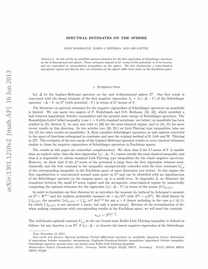
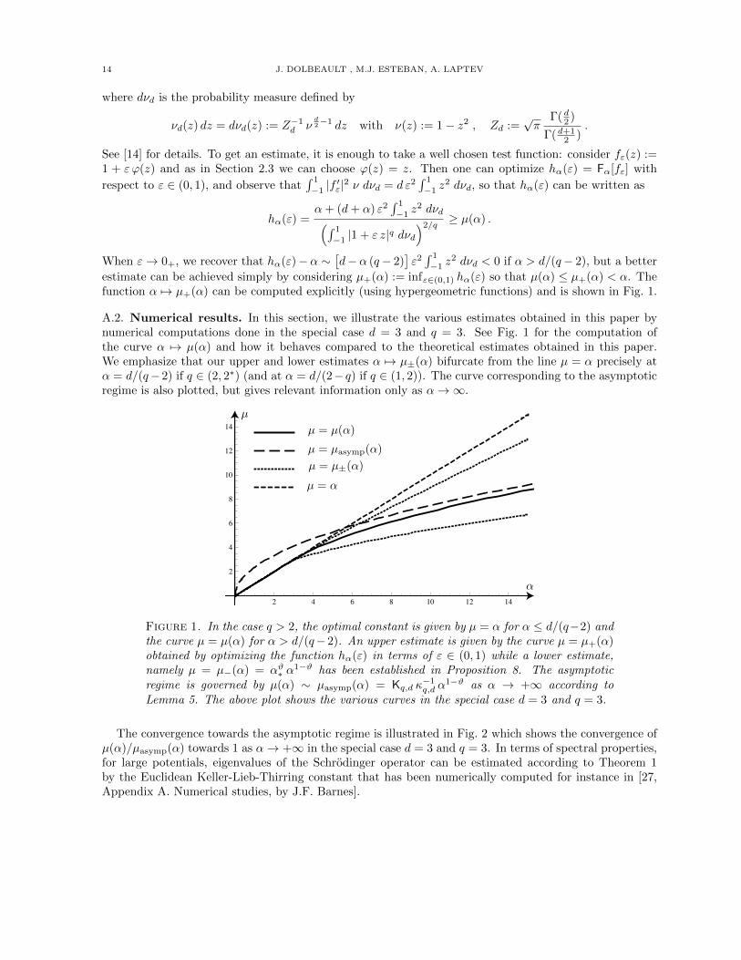
A.2. Numerical results. In this section, we illustrate the various estimates obtained in this paper bynumerical computations done in the special case d = 3 and q = 3. See Fig. 1 for the computation ofthe curve α 7→ µ(α) and how it behaves compared to the theoretical estimates obtained in this paper.We emphasize that our upper and lower estimates α 7→ µ±(α) bifurcate from the line µ = α precisely atα = d/(q− 2) if q ∈ (2, 2∗) (and at α = d/(2− q) if q ∈ (1, 2)). The curve corresponding to the asymptoticregime is also plotted, but gives relevant information only as α→∞.

2 4 6 8 10 12 14

2

4

6

8

10

12

14

α

µ

µ = µ(α)

µ = α

µ = µ±(α)

µ = µasymp(α)

Figure 1. In the case q > 2, the optimal constant is given by µ = α for α ≤ d/(q−2) andthe curve µ = µ(α) for α > d/(q−2). An upper estimate is given by the curve µ = µ+(α)obtained by optimizing the function hα(ε) in terms of ε ∈ (0, 1) while a lower estimate,namely µ = µ−(α) = αϑ∗ α

1−ϑ has been established in Proposition 8. The asymptoticregime is governed by µ(α) ∼ µasymp(α) = Kq,d κ

−1q,d α

1−ϑ as α → +∞ according toLemma 5. The above plot shows the various curves in the special case d = 3 and q = 3.

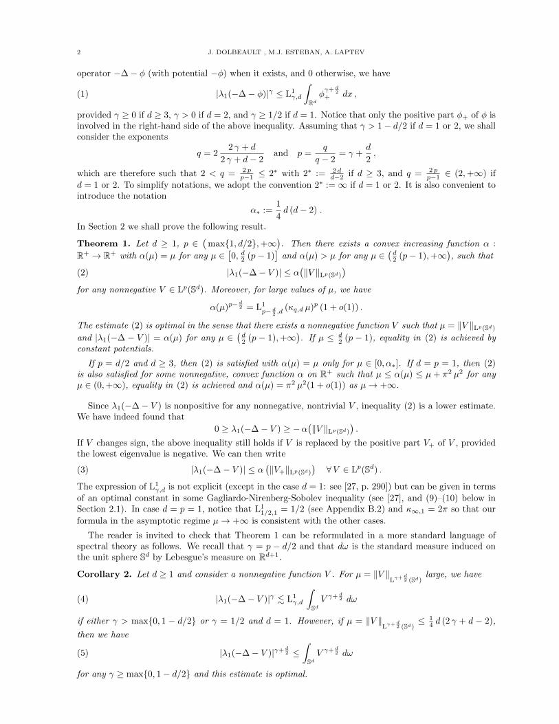
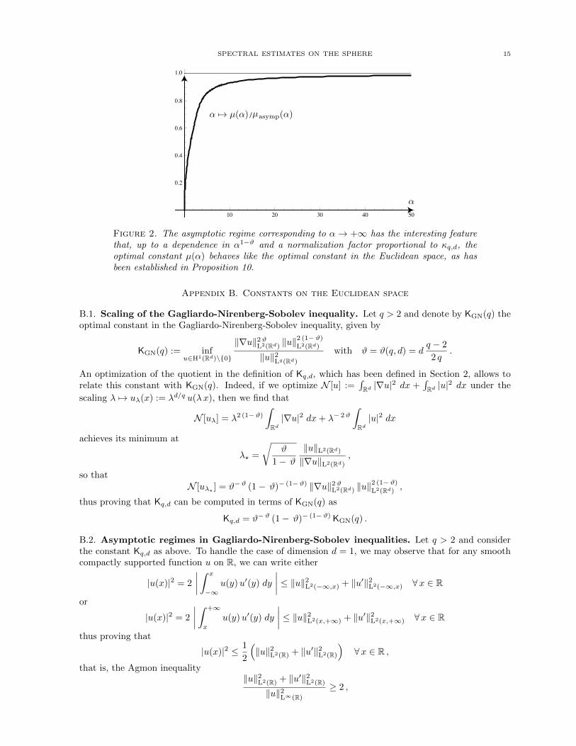
The convergence towards the asymptotic regime is illustrated in Fig. 2 which shows the convergence ofµ(α)/µasymp(α) towards 1 as α→ +∞ in the special case d = 3 and q = 3. In terms of spectral properties,for large potentials, eigenvalues of the Schrodinger operator can be estimated according to Theorem 1by the Euclidean Keller-Lieb-Thirring constant that has been numerically computed for instance in [27,Appendix A. Numerical studies, by J.F. Barnes].


10 20 30 40 50

0.2

0.4

0.6

0.8

1.0

α

α �→ µ(α) asymp(α)µ

Figure 2. The asymptotic regime corresponding to α → +∞ has the interesting featurethat, up to a dependence in α1−ϑ and a normalization factor proportional to κq,d, theoptimal constant µ(α) behaves like the optimal constant in the Euclidean space, as hasbeen established in Proposition 10.

Appendix B. Constants on the Euclidean space

B.1. Scaling of the Gagliardo-Nirenberg-Sobolev inequality. Let q > 2 and denote by KGN(q) theoptimal constant in the Gagliardo-Nirenberg-Sobolev inequality, given by

KGN(q) := infu∈H1(Rd)\{0}

‖∇u‖2ϑL2(Rd) ‖u‖2 (1−ϑ)

L2(Rd)

‖u‖2Lq(Rd)

with ϑ = ϑ(q, d) = dq − 2

2 q.

An optimization of the quotient in the definition of Kq,d, which has been defined in Section 2, allows torelate this constant with KGN(q). Indeed, if we optimize N [u] :=

∫Rd |∇u|2 dx +

∫Rd |u|2 dx under the

scaling λ 7→ uλ(x) := λd/q u(λx), then we find that

N [uλ] = λ2 (1−ϑ)

∫Rd|∇u|2 dx+ λ− 2ϑ

∫Rd|u|2 dx

achieves its minimum at

λ? =

√ϑ

1− ϑ

‖u‖L2(Rd)

‖∇u‖L2(Rd)

,

so thatN [uλ? ] = ϑ−ϑ (1− ϑ)− (1−ϑ) ‖∇u‖2ϑL2(Rd) ‖u‖

2 (1−ϑ)

L2(Rd),

thus proving that Kq,d can be computed in terms of KGN(q) as

Kq,d = ϑ−ϑ (1− ϑ)− (1−ϑ) KGN(q) .

B.2. Asymptotic regimes in Gagliardo-Nirenberg-Sobolev inequalities. Let q > 2 and considerthe constant Kq,d as above. To handle the case of dimension d = 1, we may observe that for any smoothcompactly supported function u on R, we can write either

|u(x)|2 = 2

∣∣∣∣ ∫ x

−∞u(y)u′(y) dy

∣∣∣∣ ≤ ‖u‖2L2(−∞,x) + ‖u′‖2L2(−∞,x) ∀x ∈ R

or

|u(x)|2 = 2

∣∣∣∣ ∫ +∞

x

u(y)u′(y) dy

∣∣∣∣ ≤ ‖u‖2L2(x,+∞) + ‖u′‖2L2(x,+∞) ∀x ∈ R

thus proving that

|u(x)|2 ≤ 1

2

(‖u‖2L2(R) + ‖u′‖2L2(R)

)∀x ∈ R ,

that is, the Agmon inequality‖u‖2L2(R) + ‖u′‖2L2(R)

‖u‖2L∞(R)

≥ 2 ,


and hence K∞,1 ≥ 2. Equality is achieved by the function u(x) = e−|x|, x ∈ R, and we have shown that

K∞,1 = 2 .

Proposition 15. Assume that q > 2. For all d ≥ 1,

limq→2+

Kq,d = 1

and, for all d ≥ 3,

limq→2∗

Kq,d = Sd

where Sd is the best constant in inequality (8). If d = 1, then limq→+∞ Kq,1 = K∞,1.

Proof. For any v ∈ H1(Rd) and d ≥ 3, we have

limq→2∗

‖∇v‖2L2(Rd) + ‖v‖2L2(Rd)

‖v‖2Lq(Rd)

≥ limq→2∗

‖∇v‖2L2(Rd)

‖v‖2Lq(Rd)

=‖∇v‖2L2(Rd)

‖v‖2L2∗ (Rd)

≥ Sd ,

thus proving that limq→2∗ Kq,d ≥ Sd. On the other hand, we may use the Aubin-Talenti function

(21) u(x) = (1 + |x|2)−d−22 ∀x ∈ Rd

as test function for Kq,d if d ≥ 5, i.e.

Kq,d ≤ ϑ−ϑ (1− ϑ)− (1−ϑ)‖∇u‖2ϑL2(Rd) ‖u‖

2 (1−ϑ)

L2(Rd)

‖u‖2Lq(Rd)

and observe that the right-hand side converges to Sd since limq→2∗ ϑ(q, d) = 1. If d = 3 or 4, standardadditionnal truncations are needed. The case corresponding to q →∞, d = 1 is dealt with as above.

Now we investigate the limit as q → 2+. For any v ∈ H1(Rd), we have

limq→2+

‖∇v‖2L2(Rd) + ‖v‖2L2(Rd)

‖v‖2Lq(Rd)

≥ limq→2+

‖v‖2L2(Rd)

‖v‖2Lq(Rd)

= 1 ,

thus proving that limq→2+ Kq,d ≥ 1, and for any v ∈ H1(Rd), the right-hand side in

Kq,d ≤ ϑ−ϑ (1− ϑ)− (1−ϑ)‖∇v‖2ϑL2(Rd) ‖v‖

2 (1−ϑ)

L2(Rd)

‖v‖2Lq(Rd)

converges to 1 as q → 2+. This completes the proof. �

B.3. Stereographic projection. On Sd ⊂ Rd+1, we can introduce the coordinates y = (ρ φ, z) ∈ Rd×Rsuch that ρ2 + z2 = 1, z ∈ [−1, 1], ρ ≥ 0 and φ ∈ Sd−1, and consider the stereographic projection

Σ : Sd\{N} → Rd defined by Σ(y) = x where, using the above notations, x = r φ with r =√

(1 + z)/(1− z)for any z ∈ [−1, 1). In this setting the North Pole N corresponds to z = 1 (and is formally sent at infinity)while the equator (corresponding to z = 0) is sent onto the unit sphere Sd−1 ⊂ Rd. Hence x ∈ Rd is suchthat r = |x|, φ = x

|x| , and we have the useful formulae

z =r2 − 1

r2 + 1= 1− 2

r2 + 1, ρ =

2 r

r2 + 1.

With these notations in hand, we can transform any function u on Sd into a function v on Rd using

u(y) =(rρ

) d−22 v(x) =

(r2+1

2

) d−22 v(x) = (1− z)− d−2

2 v(x)

and a painful but straightforward computation shows that, with α∗ = 14 d (d− 2),∫

Sd|∇u|2 dω + α∗

∫Sd|u|2 dω =

∫Rd|∇v|2 dx and

∫Sd|u|q dω =

∫Rd|v|q

(2

1+|x|2)d−(d−2) q2 dx .

As a consequence, Inequalities (11) and (19) are transformed respectively into∫Rd|∇v|2 dx+4 (α−α∗)

∫Rd|v|2 dx

(1 + |x|2)2≥ µ(α)κq,d

[ ∫Rd|v|q

(2

1+|x|2)d−(d−2) q2

dx

] 2q

∀ v ∈ D1,2(Rd)


if q ∈ (2, 2∗) and α ≥ α∗, and∫Rd|∇v|2 dx+ β κq,d

[ ∫Rd|v|q

(2

1+|x|2)d−(d−2) q2

dx

] 2q

≥ 4 (ν(β) +α∗)∫Rd|v|2 dx

(1 + |x|2)2∀ v ∈ D1,2(Rd)

if q ∈ (1, 2) and β > 0.

B.4. Sobolev’s inequality: expression of the constant and references. The proof that Sobolev’sinequality (8) becomes an equality if and only if u = u given by (21) up to a multiplication by a constant,a translation and a scaling is due to T. Aubin and G. Talenti: see [2, 34]. However, G. Rosen in [32]showed (by linearization) that the function given by (21) is a local minimum when d = 3 and computedthe critical value.

Much earlier, G. Bliss in [10] (also see [18]) established that, among radial functions, the followinginequality holds (∫

Rd|f |p |x|r+1−d−p dx

) 2p

≤ CBliss

∫Rd|∇f |2 |x|1−d dx

when r = p2 − 1. With the change of variables f(x) = v

(|x|− 1

d−2 x|x|

), the inequality is changed into(∫

Rd|v| 2d

d−2 dx

) d−2d

≤ CBliss

(d− 2)2 d−1d

∫Rd|∇v|2 dx

if p = 2∗ and it is a straightforward consequence of [10] that the equality is achieved with v = u.

According to the duplication formula (see for instance [1]) for the Γ function, we know that

Γ(x) Γ(x+ 1

2

)= 21− 2 x

√π Γ(2x) .

As a consequence, the best constant in Sobolev’s inequality (8) can be written either as

Sd =4

d (d− 2) |Sd|2/d

where the surface of the d-dimensional unit sphere is given by |Sd| = 2πd+12 /Γ

(d+1

2

)(see for instance [5]),

or as

Sd =1

π d (d− 2)

(Γ(d)

Γ( d2 )

) 2d

according to [2, 10, 32, 34]. This last expression can easily be recovered using the fact that optimalityin (8) is achieved by u defined in (21), while the first one, namely 1/Sd = 1

4 d (d − 2)κ2∗,d, is an easyconsequence of the stereographic projection and the computations of Section B.3 with α = α∗ and q = 2∗.

B.5. A proof of (10). Assume that q > 2 and let us relate the optimal constant L1γ,d in the one bound state

Keller-Lieb-Thirring inequality (1) with the optimal constant Kq,d in the Gagliardo-Nirenberg-Sobolev

inequality (9). In this case, recall that p = qq−2 = γ + d

2 . For any nonnegative function φ defined on Rd

such that ‖φ‖Lp(Rd) = Kq,d, using Holder’s inequality we can write that∫Rd

(|∇v|2 − φ |v|2

)dx ≥ ‖∇v‖2L2(Rd) − ‖φ‖Lp(Rd) ‖v‖2Lq(Rd)

for any v ∈ H1(Rd). Using (9), namely

‖∇v‖2L2(Rd) − Kq,d ‖v‖2Lq(Rd) ≥ −‖v‖2L2(Rd) ,

this proves that

(22) |λ1(−∆− φ)| ≤ 1 ∀φ ∈ Lp(Rd) such that ‖φ‖Lp(Rd) = Kq,d .

Next one can observe that inequality (1) can be rephrased as

L1γ,d = sup

φ∈Lp(Sd)

supv∈H1(Rd)\{0}

(R[v, φ]

)γwith R[v, φ] :=

∫Rd(φ |v|2 − |∇v|2

)dx

‖v‖2L2(Rd)

‖φ‖2 p

2 p−dLp(Rd)


where p = γ + d/2 so that the exponent 2 p2 p−d is precisely the one for which we get the scaling invariance

of R. Indeed, with vλ(x) := v(λx) and φλ(x) := φ(λx), we get that R[vλ, λ2 φλ] = R[v, φ] for any λ > 0.

Hence we find that

supv∈H1(Rd)\{0}

R[v, φ] =|λ1(−∆− φ)|‖φ‖

2 p2 p−dLp(Rd)

= supv∈H1(Rd)\{0}

R[vλ, λ2 φλ] =

|λ1(−∆− λ2 φλ)|‖λ2 φλ‖

2 p2 p−dLp(Rd)

and if we choose λ such that

λ2 p−dp ‖φ‖Lp(Rd) = ‖λ2 φλ‖Lp(Rd) = Kq,d ,

we obtain|λ1(−∆− φ)|‖φ‖

2 p2 p−dLp(Rd)

≤ 1

K2 p

2 p−dq,d

using (22), which proves that L1γ,d ≤ (Kq,d)

− pwith p = γ + d

2 . Since optimality can be preserved at each

step, this actually proves (10).

See [22, 27, 35, 36, 6, 15] for further details. In the Euclidean case, notice that the equivalence can beextended to the case of systems on the one hand and to Lieb-Thirring inequalities on the other hand: see[27, 29, 15].

B.6. A proof of (18). As in [15], we can also relate L1−γ,d and K∗q,d when q = 2 2 γ−d

2 γ−d+2 takes values

in (0, 2). The method is similar to that of Appendix B.5. For any function v ∈ H1(Rd) such that vq isintegrable and any positive potential φ such that φ−1 is in Lp(Rd) with p = q/(2− q), we can use Holder’sinequality as in the proof of Theorem 3 and get∫

Rd

(|∇v|2 + φ |v|2

)dx ≥ ‖∇v‖2L2(Rd) +

‖v‖2Lq(Rd)

‖φ−1‖Lp(Rd)

.

Using (17), namely ‖∇v‖2L2(Rd) + ‖v‖2Lq(Rd) ≥ K∗q,d ‖v‖2L2(Rd), this proves that

λ1(−∆ + φ) ≥ K∗q,d ∀φ ∈ Lp(Rd) such that ‖φ−1‖Lp(Rd) = 1 .

Inequality (6) can be rephrased as

L1− γ,d = sup

φ∈Lp(Sd)

supv∈H1(Rd)\{0}

(R[v, φ])−γ

with R[v, φ] :=

∫Rd(|∇v|2 + φ |v|2

)dx

‖v‖2L2(Rd)

‖φ−1‖p/γLp(Rd)

with γ = p+ d2 . The same scaling as in Appendix B.5 applies: with vλ(x) := v(λx) and φλ(x) := φ(λx),

we get that R[vλ, λ2 φλ] = R[v, φ] for any λ > 0 and hence

L1− γ,d =

(K∗q,d

)−γ,

which completes the proof of (18).

Acknowledgements. J.D. and M.J.E. have been partially supported by ANR grants CBDif and NoNAP.They thank the Mittag-Leffler Institute, where part of this research was carried out, for hospitality.

c© 2013 by the authors. This paper may be reproduced, in its entirety, for non-commercial purposes.

References

[1] M. Abramowitz and I. A. Stegun, Handbook of mathematical functions with formulas, graphs, and mathematical ta-

bles, vol. 55 of National Bureau of Standards Applied Mathematics Series, U.S. Government Printing Office, Washington,D.C., 1964.

[2] T. Aubin, Problemes isoperimetriques et espaces de Sobolev, J. Differential Geometry, 11 (1976), pp. 573–598.[3] D. Bakry, Functional inequalities for Markov semigroups, in Probability measures on groups: recent directions and

trends, Tata Inst. Fund. Res., Mumbai, 2006, pp. 91–147.

[4] D. Bakry and M. Ledoux, Sobolev inequalities and Myers’s diameter theorem for an abstract Markov generator, DukeMath. J., 85 (1996), pp. 253–270.

[5] W. Beckner, Sharp Sobolev inequalities on the sphere and the Moser-Trudinger inequality, Ann. of Math. (2), 138(1993), pp. 213–242.


[6] R. D. Benguria and M. Loss, Connection between the Lieb-Thirring conjecture for Schrodinger operators and anisoperimetric problem for ovals on the plane, in Partial differential equations and inverse problems, vol. 362 of Contemp.

Math., Amer. Math. Soc., Providence, RI, 2004, pp. 53–61.

[7] A. Bentaleb and S. Fahlaoui, Integral inequalities related to the Tchebychev semigroup, Semigroup Forum, 79 (2009),pp. 473–479.

[8] , A family of integral inequalities on the circle S1, Proc. Japan Acad. Ser. A Math. Sci., 86 (2010), pp. 55–59.

[9] M.-F. Bidaut-Veron and L. Veron, Nonlinear elliptic equations on compact Riemannian manifolds and asymptoticsof Emden equations, Invent. Math., 106 (1991), pp. 489–539.

[10] G. Bliss, An integral inequality, Journal of the London Mathematical Society, 1 (1930), p. 40.

[11] C. Brouttelande, The best-constant problem for a family of Gagliardo-Nirenberg inequalities on a compact Riemann-ian manifold, Proc. Edinb. Math. Soc. (2), 46 (2003), pp. 117–146.

[12] , On the second best constant in logarithmic Sobolev inequalities on complete Riemannian manifolds, Bull. Sci.Math., 127 (2003), pp. 292–312.

[13] J. Dolbeault and M. J. Esteban, Extremal functions for Caffarelli-Kohn-Nirenberg and logarithmic Hardy inequali-

ties, Proceedings of the Royal Society of Edinburgh, Section: A Mathematics, 142 (2012), pp. 745–767.[14] J. Dolbeault, M. J. Esteban, M. Kowalczyk, and M. Loss, Sharp interpolation inequalities on the sphere : new

methods and consequences, Chin. Ann. Math. Series B, 34 (2013), pp. 1–14.

[15] J. Dolbeault, P. Felmer, M. Loss, and E. Paturel, Lieb-Thirring type inequalities and Gagliardo-Nirenberg in-equalities for systems, J. Funct. Anal., 238 (2006), pp. 193–220.

[16] P. Federbush, Partially alternate derivation of a result of Nelson, Journal of Mathematical Physics, 10 (1969), pp. 50–

52.[17] P. Funk, Beitrage zur Theorie der Kegelfunktionen, Math. Ann., 77 (1915), pp. 136–162.

[18] G. H. Hardy and J. E. Littlewood, Notes on the theory of series (xii): On certain inequalities connected with the

calculus of variations, Journal of the London Mathematical Society, s1-5 (1930), pp. 34–39.

[19] E. Hecke, Uber orthogonal-invariante Integralgleichungen, Math. Ann., 78 (1917), pp. 398–404.

[20] A. A. Ilyin, Lieb-Thirring inequalities on the N-sphere and in the plane, and some applications, Proc. London Math.Soc. (3), 67 (1993), pp. 159–182.

[21] A. A. Ilyin, Lieb-Thirring inequalities on some manifolds, J. Spectr. Theory, 2 (2012), pp. 57–78.

[22] J. B. Keller, Lower bounds and isoperimetric inequalities for eigenvalues of the Schrodinger equation, J. MathematicalPhys., 2 (1961), pp. 262–266.

[23] M. Ledoux, The geometry of Markov diffusion generators, Ann. Fac. Sci. Toulouse Math. (6), 9 (2000), pp. 305–366.

Probability theory.[24] D. Levin, On some new spectral estimates for Schrodinger-like operators, Cent. Eur. J. Math., 4 (2006), pp. 123–137.

[25] D. Levin and M. Solomyak, The Rozenblum-Lieb-Cwikel inequality for Markov generators, J. Anal. Math., 71 (1997),pp. 173–193.

[26] E. Lieb, Bounds on the eigenvalues of the Laplace and Schroedinger operators, Bull. Amer. Math. Soc., 82 (1976),

pp. 751–753.[27] E. Lieb and W. Thirring, E. Lieb, B. Simon, A. Wightman Eds., Princeton University Press, 1976, ch. Inequalities for

the moments of the eigenvalues of the Schrodinger Hamiltonian and their relation to Sobolev inequalities, pp. 269–303.

[28] E. H. Lieb, Sharp constants in the Hardy-Littlewood-Sobolev and related inequalities, Ann. of Math. (2), 118 (1983),pp. 349–374.

[29] , On characteristic exponents in turbulence, Commun. Math. Phys., 92 (1984), pp. 473–480.

[30] C. E. Mueller and F. B. Weissler, Hypercontractivity for the heat semigroup for ultraspherical polynomials and onthe n-sphere, J. Funct. Anal., 48 (1982), pp. 252–283.

[31] E. M. Ouhabaz and C. Poupaud, Remarks on the Cwikel-Lieb-Rozenblum and Lieb-Thirring estimates for Schrodingeroperators on Riemannian manifolds, Acta Appl. Math., 110 (2010), pp. 1449–1459.

[32] G. Rosen, Minimum value for c in the Sobolev inequality ‖φ3‖ ≤ c ‖∇φ‖3, SIAM J. Appl. Math., 21 (1971), pp. 30–32.

[33] O. S. Rothaus, Logarithmic Sobolev inequalities and the spectrum of Schrodinger operators, J. Funct. Anal., 42 (1981),pp. 110–120.

[34] G. Talenti, Best constant in Sobolev inequality, Ann. Mat. Pura Appl. (4), 110 (1976), pp. 353–372.[35] E. J. M. Veling, Lower bounds for the infimum of the spectrum of the Schrodinger operator in RN and the Sobolev

inequalities, J. Inequal. Pure Appl. Math., 3 (2002), pp. Article 63, 22 pp. (electronic).

[36] , Corrigendum on [35], J. Inequal. Pure Appl. Math., 4 (2003), pp. Article 109, 2 pp. (electronic).

J. Dolbeault & M.J. Esteban: Ceremade CNRS UMR 7534, Universite Paris-Dauphine, Place de Lattre de

Tassigny, 75775 Paris Cedex 16, France. E-mail addresses: [email protected], [email protected]

A. Laptev: Department of Mathematics, Imperial College London, Huxley Building, 180 Queen’s Gate, Lon-

don SW7 2AZ, UK. E-mail address: [email protected]

Spectral estimates on the sphere

Documents