Estimates of Ocean Macro-turbulence: Structure Function and Spectral Slope from Argo Profiling Floats

Generated using version 3.2 of the official AMS LATEX template

Estimates of Ocean Macro-turbulence: Structure Function and1

Spectral Slope from Argo Profiling Floats2

Katherine McCaffrey ∗

National Oceanic and Atmospheric Administration, Earth Systems Research Laboratory,

Physical Sciences Division, Boulder, CO 80305, USA

3

and Baylor Fox-Kemper

Department of Earth, Environmental, and Planetary Sciences, Brown University, Providence, RI 02912, USA

Cooperative Institute for Research in Environmental Sciences, Boulder, CO 80309, USA

Gael Forget

Program in Atmospheres, Oceans and Climate, Massachusetts Institute of Technology, Cambridge, MA 02139, USA

4

∗Corresponding author address: Katherine Lynn McCaffrey (formerly of the University of Colorado atBoulder), NOAA-ESRL, 325 Broadway, Boulder 80305. E-mail: [email protected]

1

ABSTRACT5

The Argo profiling float network has repeatedly sampled much of the world’s ocean. This6

study uses Argo temperature and salinity data to form the tracer structure function of7

ocean variability at the macro-scale (10 − 1000 km, mesoscale and above). Here, second-8

order temperature and salinity structure functions over horizontal separations are calculated9

along either pressure or potential density surfaces, which allows analysis of both active and10

passive tracer structure functions. Using Argo data, a map of global variance is created11

from the climatological average and each datum. When turbulence is homogeneous, the12

structure function slope from Argo can be related to the wavenumber spectrum slope in ocean13

temperature or salinity variability. This first application of structure function techniques to14

Argo data gives physically meaningful results based on bootstrapped confidence intervals,15

showing geographical dependence of the structure functions with slopes near 23

on average,16

independent of depth.17

1

1. Introduction18

Understanding the nature of the turbulent processes in the atmosphere and ocean is19

crucial to determining large-scale circulation, and therefore climate prediction, but the re-20

lationship between large-scale circulation and small-scale turbulence is poorly understood.21

Atmospheric turbulence has been studied through spectral and structure function analyses22

for decades (Nastrom and Gage 1985; Lindborg 1999; Frehlich and Sharman 2010), and23

the results have been duplicated by high resolution General Circulation Models (GCMs)24

and mesoscale Numerical Weather Prediction (NWP) models as well (Koshyk and Hamilton25

2001; Skamarock 2004; Frehlich and Sharman 2004; Takahashi et al. 2006; Hamilton et al.26

2008). As realistic ocean climate models become increasingly turbulent, a similar dataset to27

the Nastrom and Gage spectrum would be a useful evaluation tool.28

It is often assumed that constraining a horizontal power spectral density curve, or spec-29

trum, requires a nearly-continuous synoptic survey, such as by satellite (Scott and Wang30

2005), tow-yo (Rudnick and Ferrari 1999), ship (Callies and Ferrari 2013), or glider (Cole31

and Rudnick 2012). Near-surface spectra from tow-yo and satellite have been studied by32

the authors and collaborators among many others (Fox-Kemper et al. 2011), but a similar33

comprehensive analysis has not been done deeper than 1000 m because of the limited avail-34

ability of continuous observations. However, the recent atmospheric rawinsonde method of35

Frehlich and Sharman (2010) demonstrates that a collection of individual observations may36

be used to form the structure function, which is closely related to the power spectrum in37

stationary, isotropic, homogeneous turbulence. Bennett (1984) also used balloon soundings38

to determine the local versus non-local dynamics in the atmosphere. Furthermore, struc-39

ture function analysis is quite common in the engineering literature on turbulence (She and40

Leveque 1994, is a well-known example).41

With the increased density of Argo profiling floats sampling down to 2000 m over the past42

two decades, as well as the success of the rawinsonde method in the atmosphere, this method43

is attempted to quantify large-scale (> 10 km) turbulence in the oceans. Roullet et al. (2014)44

2

recently used Argo to compute maps of eddy available potential energy to a similar end,45

but with a different method that doesn’t specify the interactions of scales and turbulence46

cascades. The structure function statistic is a useful constraint on high-resolution models,47

as structure functions are easy to calculate in a model from even a single output snapshot.48

In this study, temperature and salinity data from Argo are used to characterize large-scale49

turbulence at depth by constructing structure functions and, when relevant, inferring the50

related temperature and salinity variance spectra.51

2. Framework52

Ocean surface observations suggest that the spectral behavior for scales larger than about53

1 km differs from smaller scale turbulence (e.g., Hosegood et al. 2006). Here, we call variabil-54

ity at scales between 10 and 104 km “macro-turbulence” to emphasize that, aside from being55

large scale (meso-scale and larger), little is known about which turbulent regime is being56

observed (see also Forget and Wunsch (2007)). While dynamical frameworks for mesoscale,57

quasi-geostrophic turbulence spanning this range of scales are heavily studied at sub-inertial58

frequencies, they may not fully describe the composite nature of observed variability seen59

in real ocean data. Macro-turbulence as defined above includes mesoscale eddy activity, in-60

ternal waves, and other signals such as responses to atmospheric forcing. A complementary61

approach is to distinguish amongst observed macro-turbulence according to its spatial scale.62

To this end, structure functions provide an adequate tool that is here applied to in situ63

profiles of salinity collected by the global array of Argo floats.64

a. Structure Function - Spectrum Relationship65

The tracer autocorrelation function, Rθ is a statistical measure of the similarity (or66

difference) between a given location x and another location separated from x by the distance67

vector s, and is generally defined as68

3

Rθ(s,x) = θ′(x)θ′(x + s), (1)

where θ is a generic tracer, usually conserved, (e.g., potential temperature or salinity), the69

prime symbol denotes its deviation from an appropriate mean, and the overbar denotes70

averaging. The nth-order tracer structure function, Dθ,n, is accordingly defined as71

Dθ,n(s,x) = (θ(x)− θ(x + s))n, (2)

and its n = 2 form is simply related to the autocorrelation function by72

Dθ,2(s,x) = 2(θ′2 −Rθ(s,x)

)(3)

for homogeneous turbulence. In the case of isotropic turbulence, Rθ and Dθ,n both are in-73

dependent of direction (e.g., Dθ,n(s,x) = Dθ,n(s,x)), and for homogeneous and isotropic74

turbulence, they are further independent of x (e.g., Dθ,n(s,x) = Dθ,n(s)). Estimating75

Dθ(s) = Dθ,2(s) and exploiting the relationship in Equation (3) is of primary interest. Higher76

order structure functions can be revealing of subtle aspects of intermittency and the dissipa-77

tion of energy and variance (Kraichnan 1994) and structure-function-like statistics formed78

from the combination of velocity and tracer correlations are potentially challenging tests for79

statistical theories of turbulence (Yaglom 1949). Unfortunately, the accuracy and data re-80

quired for estimation of these statistics is beyond that of the second order structure function,81

which as we will see is rather noisy in the ocean. Also, the assumptions of homogeneity and82

isotropy will not be commonly satisfied in the ocean, but the presentation of theory will83

begin following these assumptions. Later they will be relaxed as far as the data quantity84

and quality allow.85

If a given homogeneous, isotropic turbulence spectrum (of energy or tracer variance)86

has power-law behavior over a range of wavenumbers between the energy injection and87

dissipation scales, then a related scaling law for the structure function is expected (Webb88

4

1964). Suppose the spectrum’s power law is given by B(k) = αBkλ, with spectral slope, λ.89

The structure function will also have a polynomial form: Dθ(s) = cDsγ + C0 with structure90

function slope, γ, and a constant C0 representing contributions from other portions of the91

spectrum not adhering to the B(k) = αBkλ law (shown to be negligible in Webb (1964)).92

The relationship between the two slopes (derived in Appendix A) is93

γ = −λ− 1. (4)

However, structure functions calculated here often have a bend point with two slopes, so94

an analysis is needed to determine whether that was a sign of two separate power laws in the95

spectrum (a common example occurs in Nastrom and Gage (1985), where a spectral slope96

of λ = −53

is seen below 500 km, and λ = −3 is seen above 500 km). As shown in Appendix97

A, if spectral slopes of the two power-law scalings are λ1 and λ2, then the structure function98

can be written as99

Dθ(s) = c1sγ1 + c2s

γ2 , (5)

where the same relationship between structure function slope, γ, and spectral slope, λ,100

i.e. Equation (4), applies between the large scale structure function slope versus small101

wavenumber spectral slope, and for the small scale structure function slope versus large102

wavenumber spectral slope. As long as the inertial range over which each power law applies103

is large enough and γ1 < γ2, the first term dominates the small scale, and the second term104

dominates the large scales.105

Observational estimates of structure functions often, and expectedly, show flat slopes106

at extreme separation distances. For large enough s, Equation (3) indeed predicts that107

Dθ(s → ∞) → 2θ′2 (or θ′2(x1) + θ′2(x2) in heterogeneous cases) in the limit where remote108

locations are fully uncorrelated (so that Rθ(s → ∞) → 0). For small enough s, a similar109

behavior can sometimes be seen, as the assumption of simultaneous observations can break110

down, the signal of interest goes to 0 and data noise becomes predominant. The scale of111

5

transition at which these limiting cases begin to dominate is difficult to predict, and generally112

unknown. It may be that the scale of transition is meaningful (e.g., indicating the scale of113

the largest coherent structures), but conclusive evidence of a meaningful transition generally114

requires more information that just the structure function alone. However, the matter of115

interest here is Dθ(s) within the inertial range(s), away from these limiting cases.116

A primary goal of this paper will be to estimate γ from data over length scales where a117

single power law is suspected, or both γ1 and γ2 when a single linear fit is not apparent, and118

compare it to relevant theories, reviewed below, predicting γ or a spectral equivalent.119

b. Relevant Theories120

Kolmogorov (1941) introduced the idea of an inertial range in isotropic, homogeneous tur-121

bulence through dimensional analysis, arriving at a kinetic energy spectrum of E(k) ∝ k−5/3.122

Using Kolmogorov-like dimensional arguments, Obukhov (1949) and Corrsin (1951) predict123

a temperature spectrum with slope λ = −53. Due to rotation, stratification, and limited124

total depth, large-scale (> O(10 km)) ocean flows are quasi-two-dimensional (dominantly125

horizontal), and not expected to follow the simple scalings first derived by Kolmogorov and126

Obukhov-Corrsin. Two-dimensional turbulence scalings by Kraichnan (1967) of the kinetic127

energy slope of E(k) ∝ k−3 in the enstrophy cascade range (plus a logarithmic correction128

neglected here) at small scales and E(k) ∝ k−5/3 in the inverse energy cascade at large scales129

could potentially describe barotropic motions. Batchelor (1959) and Vallis (2006) argue that130

in turbulence where each wavenumber is dominated by a single eddy-turnover timescale, a131

passive tracer spectrum should exhibit a slope of λ = −1 (γ = 0). The Obukhov and Batche-132

lor passive tracer spectra are examined in a relevant limit by Pierrehumbert (1994). Charney133

(1971), Salmon (1982), and Blumen (1978) all describe kinetic energy spectra for the quasi-134

geostrophic flows. For all cases, passive tracers should behave as Obukhov-Corrsin predict135

when E(k) ∝ k−5/3, or as the single eddy-turnover timescale result of λ = −1 (γ = 0) when136

E(k) ∝ k−3. However, the wavenumber range where these spectral slopes should appear in137

6

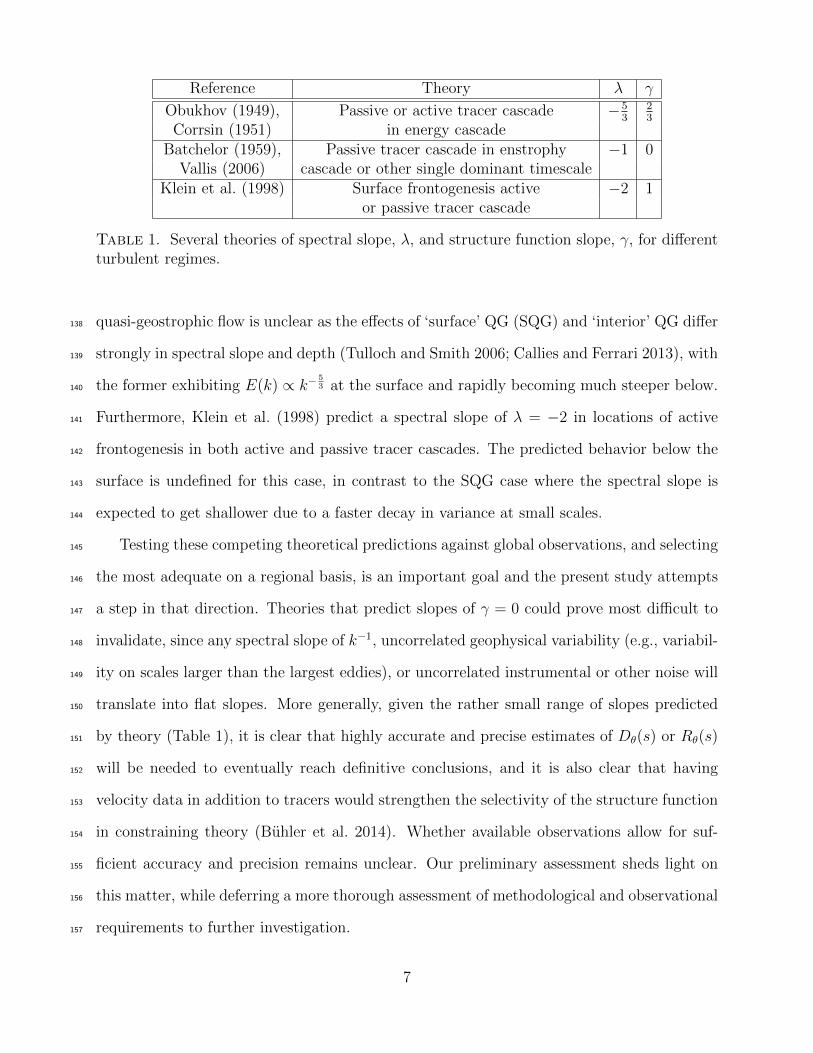
Reference Theory λ γ

Obukhov (1949), Passive or active tracer cascade −53

23

Corrsin (1951) in energy cascadeBatchelor (1959), Passive tracer cascade in enstrophy −1 0

Vallis (2006) cascade or other single dominant timescaleKlein et al. (1998) Surface frontogenesis active −2 1

or passive tracer cascade

Table 1. Several theories of spectral slope, λ, and structure function slope, γ, for differentturbulent regimes.

quasi-geostrophic flow is unclear as the effects of ‘surface’ QG (SQG) and ‘interior’ QG differ138

strongly in spectral slope and depth (Tulloch and Smith 2006; Callies and Ferrari 2013), with139

the former exhibiting E(k) ∝ k−53 at the surface and rapidly becoming much steeper below.140

Furthermore, Klein et al. (1998) predict a spectral slope of λ = −2 in locations of active141

frontogenesis in both active and passive tracer cascades. The predicted behavior below the142

surface is undefined for this case, in contrast to the SQG case where the spectral slope is143

expected to get shallower due to a faster decay in variance at small scales.144

Testing these competing theoretical predictions against global observations, and selecting145

the most adequate on a regional basis, is an important goal and the present study attempts146

a step in that direction. Theories that predict slopes of γ = 0 could prove most difficult to147

invalidate, since any spectral slope of k−1, uncorrelated geophysical variability (e.g., variabil-148

ity on scales larger than the largest eddies), or uncorrelated instrumental or other noise will149

translate into flat slopes. More generally, given the rather small range of slopes predicted150

by theory (Table 1), it is clear that highly accurate and precise estimates of Dθ(s) or Rθ(s)151

will be needed to eventually reach definitive conclusions, and it is also clear that having152

velocity data in addition to tracers would strengthen the selectivity of the structure function153

in constraining theory (Buhler et al. 2014). Whether available observations allow for suf-154

ficient accuracy and precision remains unclear. Our preliminary assessment sheds light on155

this matter, while deferring a more thorough assessment of methodological and observational156

requirements to further investigation.157

7

c. Data Analysis Techniques158

The data used in this analysis were obtained from Argo floats distributed over the world159

ocean, from 2000 to 2013. The extensive Argo float array introduced the first systematic,160

near-real time, sampling of temperature and salinity of the global ocean on a large spectrum161

of scales with accuracy of approximately .01◦C and .01 psu, respectively (Argo Science162

Team 1998). The International Argo Program currently collects and provides profiles from163

an array of 3600 floats. Each Argo float takes a vertical profile of temperature and salinity164

as it ascends from 2000 m to the surface, where it transmits the data via satellite (using165

Argos or Iridium systems) before descending and drifting for, typically, 9 days. Calibration166

and quality control is done on all profiles at one of the national data centers, and though an167

incorrect or missing calibration could skew the statistics computed here, they are assumed168

to be correct (Carval et al. 2011). In processing the data, we relied on the Argo delayed-169

mode procedures for checking sensor drifts and offsets in salinity, and made use of the Argo170

quality flags. Density was computed for each Argo temperature/salinity profile, which was171

then interpolated to standard density levels, ∼ 24.0−27.8 kg m−3 in intervals of 0.1 kg m−3,172

and standard depth levels, 5 m at the surface, with increasing intervals down to 2000 m.173

Salinity is here analyzed along either isobars or isopycnals, taken as a representative174

of active and passive tracers respectively. A reasonable alternative would be to analyze,175

e.g., temperature on isobars (active) and “spice” on isopycnals (passive), but we choose to176

follow the simplest approach for a first assessment of Argo data. In interpolating salinity to177

standard density level, potential density is computed using the Thermodynamic Equation of178

Seawater (Millero et al. 2008). The presented results, however, are largely insensitive to a179

change in assumed equation of state compared to other approximations (e.g., neutral density,180

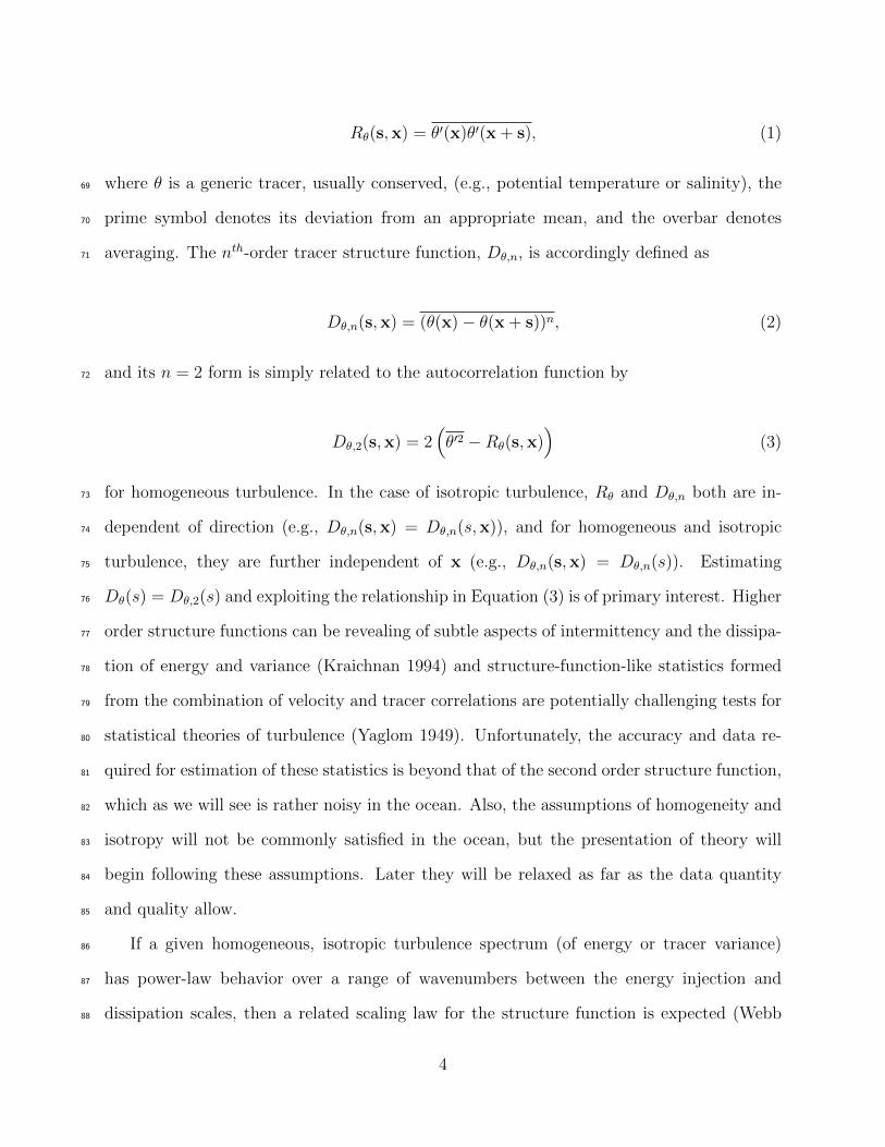
not shown). Figure 1 shows potential density from the Ocean Comprehensive Atlas (OCCA)181

climatology (Forget 2010) varying with depth in the western Atlantic (a) and central Pacific182

(b) Oceans, and highlights the σ0 = 25.8 kg m−3 and σ0 = 27.3 kg m−3 isopycnals analyzed183

in this study.184

8

Latitude

Dep

th (m

)

Atlantic

27.8

27.827.6

27.4

27.2

2726.8

26.6

25.526.4

27.8

27.627.427.22726.826.626.6

27.3

25.7

−60 −40 −20 0 20 40 60

500

1000

1500

2000

Latitude

Dep

th (m

)

Pacific

27.6

27.4

27.2

27

26.826.626.4

27.6

27.427.2

2726.826.6

26.826.6

27.6

27.4

27.227

27.327.3

27.3

25.725.7

−60 −40 −20 0 20 40 60

500

1000

1500

2000

a)

b)

Fig. 1. Potential density (in kg m−3) along 23.5W in the eastern Atlantic Ocean (a) and180W in the Pacific (b), calculated from the OCCA climatology of temperature, salinity,and pressure with the Thermodynamics Equation of Seawater. The 25.7 and 27.3 kg m−3

isopycnals are highlighted for analysis in Section 3d.

9

The global data coverage by Argo is much denser and more homogeneous than that of185

ship-based measurements. This fact, and the continued growth of the profiles database,186

motivate our focus on Argo data. As compared with, e.g., along-track altimetry, the dis-187

tribution of Argo profiles is highly irregular, as a result of the complex drifting patterns of188

a multitude of individual floats. In this context, the use of structure functions is a rather189

obvious methodological choice. Fast Fourier Transforms, for example, require data follow-190

ing a straight, regular, gap-free path (or statistical interpolation techniques to impute an191

equivalent).192

Isotropic structure functions for salinity are computed according to193

DS(s) = (S ′(x)− S ′(x+ s))2, (6)

where S ′(x) − S ′(x + s) denotes the difference in salinity anomalies for an Argo data pair194

separated by distance s, and the double overbar denotes a weighted sample average. Com-195

putations are carried out in logarithmically spaced s bins, between 10 and 10, 000 km. Other196

computational details (regarding salinity anomalies, weighted sample averages, weighting for197

unequal directional bins, and computational domains) are reported below. Isobaric structure198

function estimates are denoted as DS(s)|p, while isopycnic structure function estimates are199

denoted as DS(s)|σ.200

There are no pairs of Argo floats measuring at the exact same time, but the lack of strict201

simultaneity is not crucial. Indeed, observations that occur close enough together in time202

(∆t) and over sufficient spatial separation (s) form an effectively simultaneous pair, to the203

extent that oceanic signals cannot travel fast enough between paired observations. Thus,204

following Frehlich and Sharman (2010), data pairs such that s > cmax∆t are considered205

“effectively simultaneous,” and included in the average. An example of the probability206

distribution of ∆t and s, for observations within a given Pacific region, is shown in Figure 2.207

The trade-off involved in choosing cmax is as follows: a large cmax (e.g. 10 m s−1) reduces208

10

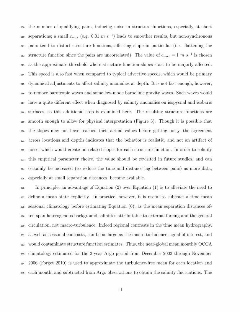
the number of qualifying pairs, inducing noise in structure functions, especially at short209

separations; a small cmax (e.g. 0.01 m s−1) leads to smoother results, but non-synchronous210

pairs tend to distort structure functions, affecting slope in particular (i.e. flattening the211

structure function since the pairs are uncorrelated). The value of cmax = 1 m s−1 is chosen212

as the approximate threshold where structure function slopes start to be majorly affected.213

This speed is also fast when compared to typical advective speeds, which would be primary214

dynamical adjustments to affect salinity anomalies at depth. It is not fast enough, however,215

to remove barotropic waves and some low-mode baroclinic gravity waves. Such waves would216

have a quite different effect when diagnosed by salinity anomalies on isopycnal and isobaric217

surfaces, so this additional step is examined here. The resulting structure functions are218

smooth enough to allow for physical interpretation (Figure 3). Though it is possible that219

the slopes may not have reached their actual values before getting noisy, the agreement220

across locations and depths indicates that the behavior is realistic, and not an artifact of221

noise, which would create un-related slopes for each structure function. In order to solidify222

this empirical parameter choice, the value should be revisited in future studies, and can223

certainly be increased (to reduce the time and distance lag between pairs) as more data,224

especially at small separation distances, become available.225

In principle, an advantage of Equation (2) over Equation (1) is to alleviate the need to226

define a mean state explicitly. In practice, however, it is useful to subtract a time mean227

seasonal climatology before estimating Equation (6), as the mean separation distances of-228

ten span heterogenous background salinities attributable to external forcing and the general229

circulation, not macro-turbulence. Indeed regional contrasts in the time mean hydrography,230

as well as seasonal contrasts, can be as large as the macro-turbulence signal of interest, and231

would contaminate structure function estimates. Thus, the near-global mean monthly OCCA232

climatology estimated for the 3-year Argo period from December 2003 through November233

2006 (Forget 2010) is used to approximate the turbulence-free mean for each location and234

each month, and subtracted from Argo observations to obtain the salinity fluctuations. The235

11

Fig. 2. Log of the joint probability distribution of pairs (color) depending on separationdistance (x-axis) and separation time (y-axis) for all observations in the heterogeneous regionin the Pacific Ocean between 10N-30N and 140W-160W. Left: all pairs of observations.Right: the pairs limited by cmax < 1 m s−1. Both plots have dotted lines showing threedifferent cmax limits with increasing line thickness: 0.01, 1, and 10 m s−1.

12

structure function average (the double-bar in Equation 6) is then computed for all simulta-236

neous pairs, independent of season, though it is possible to analyze those differences as in237

Cole and Rudnick (2012) and Figure 3.238

The structure function is a statistic that is adequate, in its own right, to describe ocean239

macro-turbulence. The slopes relation Equation (4) makes it interchangeable with power240

spectra, but only under assumptions of homogeneity and isotropy. When these assumptions241

are violated (and in practice they are never perfectly valid) the interpretation of either statis-242

tic, and of their mutual relation, becomes much more difficult. Hence caution in analyzing243

either statistic is recommended, and it is crucial to assess and possibly mitigate departures244

from homogeneity and isotropy. We note that is it possible, for statistically stationary tur-245

bulence, to reduce or remove spatial and directional averaging in Equations (1-3), retaining246

only a temporal or ensemble average, producing structure functions suitable for heteroge-247

neous and anisotropic conditions. Nonetheless, the continued growth of Argo is bound to248

allow for refined analyses in the future. The heterogeneity seen in Argo data is discussed in249

Section 3.250

In order to mitigate the impact of anisotropy, structure functions are first computed in251

directional bins, and a weighted average of directional bins is then performed (see Appendix252

B). Since structure function slope estimates are of particular interest, and to gain insight253

into their statistical significance, they are presented with bootstrap confidence intervals (see254

Appendices B and C). A detail of importance is that slope calculations should omit large255

separations, where DS expectedly asymptotes to 2θ′2. To this end, a bend point is determined256

in DS and slopes are computed below the bend point (Appendix D).257

13

3. Structure Function Results258

a. Preliminary Assessment259

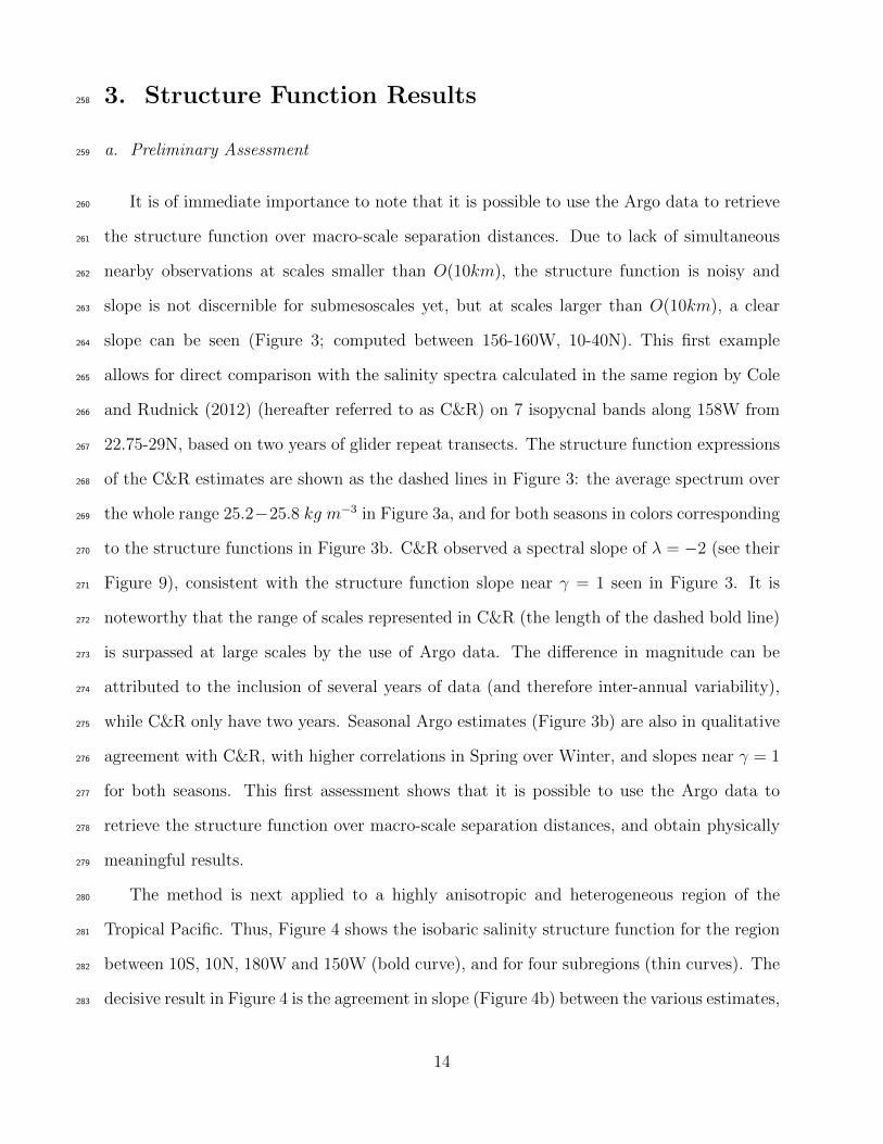
It is of immediate importance to note that it is possible to use the Argo data to retrieve260

the structure function over macro-scale separation distances. Due to lack of simultaneous261

nearby observations at scales smaller than O(10km), the structure function is noisy and262

slope is not discernible for submesoscales yet, but at scales larger than O(10km), a clear263

slope can be seen (Figure 3; computed between 156-160W, 10-40N). This first example264

allows for direct comparison with the salinity spectra calculated in the same region by Cole265

and Rudnick (2012) (hereafter referred to as C&R) on 7 isopycnal bands along 158W from266

22.75-29N, based on two years of glider repeat transects. The structure function expressions267

of the C&R estimates are shown as the dashed lines in Figure 3: the average spectrum over268

the whole range 25.2−25.8 kg m−3 in Figure 3a, and for both seasons in colors corresponding269

to the structure functions in Figure 3b. C&R observed a spectral slope of λ = −2 (see their270

Figure 9), consistent with the structure function slope near γ = 1 seen in Figure 3. It is271

noteworthy that the range of scales represented in C&R (the length of the dashed bold line)272

is surpassed at large scales by the use of Argo data. The difference in magnitude can be273

attributed to the inclusion of several years of data (and therefore inter-annual variability),274

while C&R only have two years. Seasonal Argo estimates (Figure 3b) are also in qualitative275

agreement with C&R, with higher correlations in Spring over Winter, and slopes near γ = 1276

for both seasons. This first assessment shows that it is possible to use the Argo data to277

retrieve the structure function over macro-scale separation distances, and obtain physically278

meaningful results.279

The method is next applied to a highly anisotropic and heterogeneous region of the280

Tropical Pacific. Thus, Figure 4 shows the isobaric salinity structure function for the region281

between 10S, 10N, 180W and 150W (bold curve), and for four subregions (thin curves). The282

decisive result in Figure 4 is the agreement in slope (Figure 4b) between the various estimates,283

14

Fig. 3. a) Salinity structure function, DS(s)|σ, along 158W for 10-40N along isopycnals of25.2 − 25.8 kg m−3, 25.8 − 26.4 kg m−3, 26.4 − 26.6 kg m−3, 26.6 − 26.8 kg m−3, 26.8 −27.0 kg m−3, 27.0− 27.2 kg m−3, 27.2− 27.3 kg m−3. Dashed line is the structure functionmodel equivalent to the spectrum found by Cole and Rudnick (2012). b) Structure functionsat 25.2 − 25.8 kg m−3 for the seasons specified in C&R. April-May: red, Nov-Dec: blue.Dashed lines are the structure function model equivalent to a fit of C&R’s spectrum for theApril-May and Nov-Dec, respectively.

indicating that the four subregions are not governed by fundamentally different dynamics284

despite heterogeneity in simpler statistics (e.g. salinity variance, as plotted in Figure 5). The285

90% confidence interval, shown for the full region, is indicative of the statistical significance286

of the differences between the average and the subregion estimates. Bootstrap confidence287

intervals are expectedly wider for the data subgroups (since the sample size is smaller;288

see Table 3 in Appendix B). Despite the overall agreement, it is still possible that such289

differences could be an artifact resulting from heterogeneity and uneven sampling. The first290

order conclusion from Figure 4, however, is that robust structure function patterns (with291

confidence intervals) can emerge, even in the presence of anisotropy and heterogeneity, when292

considering regions of similar dynamics.293

Taken all together, the relative success of the two presented tests (Figures 3-4) warrants294

further investigation of Argo structure function estimates. The rest of this section thus295

proceeds to assess the dependence of Argo structure function estimates on depth, level of296

eddy energy, and latitude.297

15

s (km)102 103

DS

(s) (

psu2 )

10-3

10-2

10-1

10S-10N, 180-210W10S-Eq, 180-165W10S-Eq, 165-150WEq-10N, 180-165WEq-10N, 165-150W

a)

Slope0 0.5 1 1.5

180-150W, -10-10N

180-165W, -10-0N

165-150W, -10-0N

180-165W, 0-10N

165-150W, 0-10N

Amplitude (psu2)10-2 10-1

c)b)

Fig. 4. a) Isobaric salinity structure function at 5 m in the central Equatorial Pacificbetween 10S and 10N and 180W and 150W (dotted region in Figure 5). The bold line is thestructure function computed for the entire region, with a 90% confidence interval in grayshading, and each of the four lines is a subregion: red - 10S-Eq, 180-165W; blue - 10S-Eq,165-150W; magenta - Eq-10N, 180-165W; green - Eq-10N, 165-150W. The small scale slopes(b) and amplitudes (c) for each subregion are shown on the right, including a 90% bootstrapconfidence interval.

b. Depth Dependence298

One tantalizing aspect of the Argo data is that estimates of structure function can be299

made at depths exceeding the depth where continuous data is presently available. Glider300

and submarine data remain rare, and tow-yos at substantial depth are not feasible. Thus,301

the first analysis here concerns how the structure function estimates depend on depth.302

Beginning the assessment of ocean turbulence with the structure function as its own303

statistic, both isobaric and isopycnal structure functions are calculated at different depths,304

first in a relatively quiet region of the mid-latitude Pacific (Figures 6 & 7). This region305

shows some degree of heterogeneity in salinity variance (see Figure 5) but is far removed306

from the most energetic ocean jets (the Kuroshio and Equatorial Undercurrent in particular).307

Variance in the upper 250 m is near constant in Figure 6, which is consistent with a low308

level of eddy energy (a point further discussed in the next section).309

Both isobaric and isopycnal structure functions generally show positive slopes, with 90%310

16

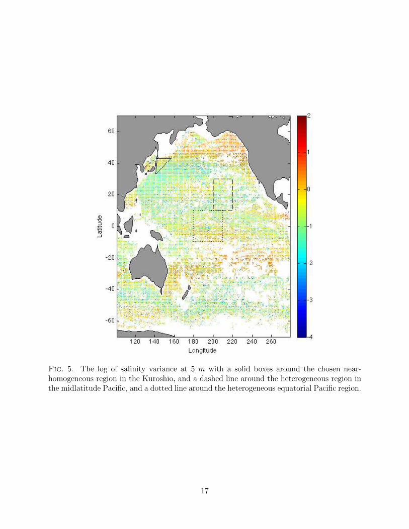
Fig. 5. The log of salinity variance at 5 m with a solid boxes around the chosen near-homogeneous region in the Kuroshio, and a dashed line around the heterogeneous region inthe midlatitude Pacific, and a dotted line around the heterogeneous equatorial Pacific region.

17

confidence based upon bootstrap distributions, and bootstrap mean slopes that are often near311

23. Differences between pressure and density surfaces can be instructive about the effects of312

internal waves and eddies on the structure function. Furthermore, since the region analyzed313

in Figures 6 and 7 is eddy-poor, isobaric structure functions may rather characterize internal314

wave activity, while structure functions computed along isopycnals are expected to filter out315

some of the internal wave signals. However, the current level of uncertainty indicated by316

bootstrap intervals is too high to draw conclusions with a high confidence on those grounds317

(Figures 6b & 7b). Additional data will be needed to reduce uncertainties and challenge318

the general behavior seen in Figures 6 & 7 – i.e. the fact that slopes are positive with 90%319

confidence, with a mean slope near 23, throughout the upper 1900 m, on isopycnals as well320

as on isobaric surfaces.321

The isobaric salinity structure function estimates in this region are relatively constant in322

amplitude (quantified as the average of the large scale fit-line) near the surface mixed layer323

(i.e., within 250 m of the surface), and then decay roughly exponentially with depth. The324

isopycnal structure function is nearly constant until a much greater depth (near 26.8 kg m−3,325

near 500 m depth), and then decays. It is tempting to compare this result to SQG theory,326

where an exponential decay with depth is predicted, and has nearly constant amplitude327

within the mixed layer. However, the slope of the structure function is consistent across all328

depths, where SQG predicts strong steepening with depth as short separation scales become329

de-correlated. As will be shown below, however, this pattern of slope and amplitude is not330

universal.331

c. Eddy-Rich vs. Eddy-Poor Regions332

A similarly contrasting, yet conclusive picture emerges when comparing regions of high333

versus low meso-scale eddy energy. In order to assess the effect of eddies on structure334

functions, the Kuroshio region, where eddy activity is very high, is compared to the eddy-335

poor region discussed above. Figure 8, based upon interpolated data distributed by Aviso336

18

101 102 103 104

10−4

10−3

10−2

10−1

100

s (km)

D S(s) (

psu2 )

m

5

500

1500

1900

−1 2 1 2

5

155

305

455

605

755

905

1055

1205

1355

1505

1655

18051900

Dep

th (m

)

Slope(psu2 km−1)

10−410−310−210−1100

Amplitude (psu2)

a) b) c)

Slope

Fig. 6. Isobaric salinity structure functions, DS(s)|p, (a) between 10-30N and 140-160W inthe Pacific Ocean (a heterogeneous region with high and low salinity variance) on pressuresurfaces (5− 1900 m, represented by color). b) Small scale slopes of the structure functionat each latitude band, including 90% bootstrap confidence interval. c) Amplitude of thethe large-scale structure function at each latitude band, including 90% bootstrap confidenceinterval. Reference slopes of γ = 0 (dashed) and 2

3(solid) are shown in bold in a and dashed

lines in b.

19

101 102 103 104

10−4

10−3

10−2

10−1

s (km)

D S(s) (

psu2 )

25.1

27.6

−1 0 1 2

25.2

25.4

25.6

25.8

26

26.2

26.4

26.6

26.8

27

27.2

27.4

27.6

Den

sity

(kg

m−3

)

Slope (psu2 km−1)

10−410−310−210−1100

Amplitude (psu2)

10−410−310−210−1100

a) b) c)

Slope

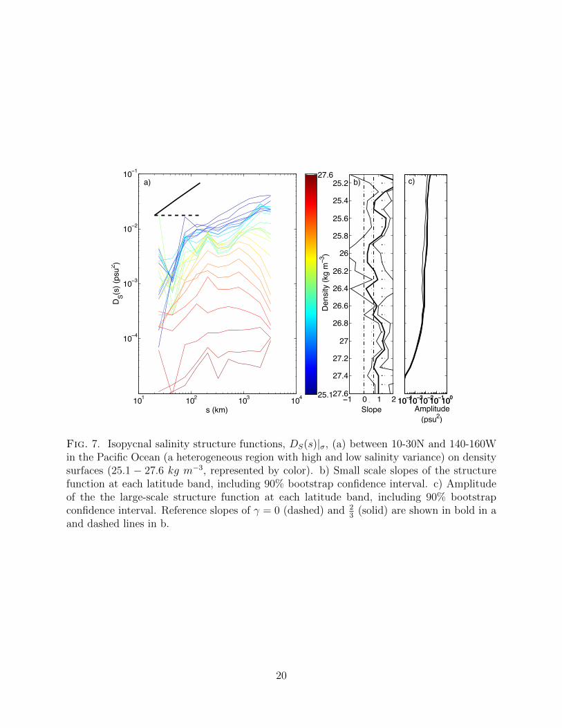
Fig. 7. Isopycnal salinity structure functions, DS(s)|σ, (a) between 10-30N and 140-160Win the Pacific Ocean (a heterogeneous region with high and low salinity variance) on densitysurfaces (25.1 − 27.6 kg m−3, represented by color). b) Small scale slopes of the structurefunction at each latitude band, including 90% bootstrap confidence interval. c) Amplitudeof the the large-scale structure function at each latitude band, including 90% bootstrapconfidence interval. Reference slopes of γ = 0 (dashed) and 2

3(solid) are shown in bold in a

and dashed lines in b.

20

Fig. 8. Log10 of eddy kinetic energy (cm2 s−2) on the surface from AVISO satellite altimetrymeasurements from 1993-2010.

(http://www.aviso.oceanobs.com/), confirms the clear contrast in eddy energy between the337

two selected regions. In order to mitigate the impact of heterogeneity associated with the338

quieter surroundings of energetic jets, the region of analysis was further guided by the map339

of salinity variance at 5 m (Figure 5).340

Figure 9 shows much increased isobaric variance near the surface, again consistent with341

the exponential decay expected from SQG theory (see Callies and Ferrari 2013). Further-342

more, variance on isopycnals is near constant above ∼ 26.5 kg m−3, both in eddy-rich and343

eddy-poor regimes (Figures 7 & 9), and it decreases gradually below ∼ 26.5 kg m−3. If344

one takes the isobaric structure functions as indicating primarily (or dominated by) inter-345

nal waves, and the isopycnal structure function as indicating (or dominated by) geostrophic346

variability, then this result is the opposite of what is expected from popular theories: SQG347

(strong decay in isopycnal structure function) and bottom-generated internal waves (increas-348

ing variability as the bottom is approached). The increased surface variability in isobaric349

structure functions may be an indicator of strong near-inertial internal waves generated by350

winds at the surface (Kunze 1985). Again, a slope of γ ≈ 23

is seen in the Kuroshio region,351

on both isobars and isopycnals, with no obvious dependence on depth (Figure 7b & 9b ),352

21

101 102 103

10−4

10−3

10−2

10−1

100

s (km)

DS(s

) (ps

u2 )

m

200

400

600

800

1000

1200

1400

1600

1800a)

Slope-1 0 1

Dep

th (m

)

75145216286356426496566637707777847917988

1058112811981268133914091479154916191689176018301900

Amplitude (psu2)10-3 10-2 10-1

b) c)

Fig. 9. Isobaric salinity structure function, DS(s)|p, (a) in the Kuroshio uniform varianceregion at depths from 5 m to 2000 m, represented in color. b) Small scale slopes of thestructure function at each latitude band, including 90% bootstrap confidence interval. c)Amplitude of the the large-scale structure function at each latitude band, including 90%bootstrap confidence interval. Reference slopes of γ = 0 and 2

3are shown in bold in a (solid

and dashed, respectively) and dashed lines in b.

corresponding (in homogeneous turbulence) to the spectral slope of λ = −53. Figure 10 also353

adheres to this slope at all depths, but again the isopycnal structure function stays nearly354

constant until a much greater depth (26.4 kg m−3), beyond which exponential weakening355

with depth occurs.356

The γ = 23

behavior may also be described by the theory of passive tracer variance of357

Obukhov (1949) and Corrsin (1951), with structure function slopes equivalent to a spectral358

slope of λ = −53. The persistence of the γ = 2

3slope deep in the water column is an359

indicator of the energy (and therefore tracer) cascade to larger scales as a function of depth360

on isopycnals. At larger scales, the slope of γ = 0 may indicate that the structure function361

slope is uncorrelated, random motions, or that it is equivalent to a spectral slope of λ = −1,362

which coincides with the theory of Vallis (2006) of the passive tracer. This theory would363

suggest that the largest eddies are the size of the onset of the γ = 0 regime, and the bend364

point is found around 200 km.365

The fact that isobaric structure function slopes only weakly depend on depth may reflect366

22

102 10310−4

10−3

10−2

10−1

100

s (km)

D S(s) (

psu2 )

25.4

27.6

−2 0 2

25.4

25.6

25.8

26

26.2

26.4

26.6

26.8

27

27.2

27.4

27.6Slope

(psu2 km−1)

Den

sity

(kg

m−1

)

10−410−310−210−1100

Amplitude (psu2)

a) c)b)

2 0 2Slope

Fig. 10. Isopycnal salinity structure function, DS(s)|σ, (a) in the Kuroshio region, chosenas uniform on the 5 m isobar, from 25.4 to 27.6 kg m−3, represented by color. b) Small scaleslopes of the structure function at each latitude band, including 90% bootstrap confidenceinterval. c) Amplitude of the the large-scale structure function at each latitude band, in-cluding 90% bootstrap confidence interval. Reference slopes of γ = 0 and 2

3are shown in

bold in a (solid and dashed, respectively) and dashed lines in b.

23

the presence of internal waves throughout the water column. Differences between isobaric367

and isopycnal structure functions could be attributed to internal wave signals that should be368

partially omitted by construction of isopycnal structure functions. In further investigation,369

such hypotheses could be investigated by calculating predictions from, e.g., the Garrett-Munk370

spectrum (Garrett and Munk 1972) of internal waves. Such theories are still evolving, but371

would not change the diagnosis of this dataset. For more recent discussion and observations372

of the internal wave spectrum, the reader is referred to Klymak and Moum (2007) and Callies373

and Ferrari (2013).374

Figures 6-7-9-10 do not exclude the possibility that subtle differences may be found375

between eddy-rich versus eddy-poor, isopycnal versus isobaric structure functions. However,376

additional data is necessary to increase the degree of confidence and draw more definitive377

conclusions. At this stage, the null hypothesis being tested, based upon the robust behavior378

seen in Figures 6-7-9-10, is that structure function slopes are positive with high confidence379

and near 23

on average. Structure function amplitude tends to decay with depth, and more380

slowly in the isopycnal structure function than in the isobaric, but without changing the381

slope. How universal this behavior may be and the implications for theoretical work remains382

to be established.383

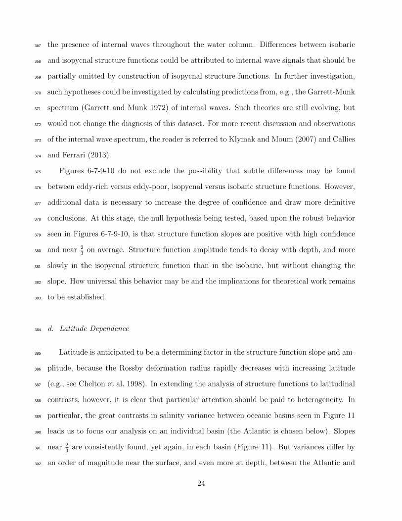
d. Latitude Dependence384

Latitude is anticipated to be a determining factor in the structure function slope and am-385

plitude, because the Rossby deformation radius rapidly decreases with increasing latitude386

(e.g., see Chelton et al. 1998). In extending the analysis of structure functions to latitudinal387

contrasts, however, it is clear that particular attention should be paid to heterogeneity. In388

particular, the great contrasts in salinity variance between oceanic basins seen in Figure 11389

leads us to focus our analysis on an individual basin (the Atlantic is chosen below). Slopes390

near 23

are consistently found, yet again, in each basin (Figure 11). But variances differ by391

an order of magnitude near the surface, and even more at depth, between the Atlantic and392

24

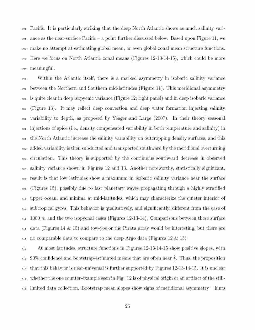
Pacific. It is particularly striking that the deep North Atlantic shows as much salinity vari-393

ance as the near-surface Pacific – a point further discussed below. Based upon Figure 11, we394

make no attempt at estimating global mean, or even global zonal mean structure functions.395

Here we focus on North Atlantic zonal means (Figures 12-13-14-15), which could be more396

meaningful.397

Within the Atlantic itself, there is a marked asymmetry in isobaric salinity variance398

between the Northern and Southern mid-latitudes (Figure 11). This meridional asymmetry399

is quite clear in deep isopycnic variance (Figure 12; right panel) and in deep isobaric variance400

(Figure 13). It may reflect deep convection and deep water formation injecting salinity401

variability to depth, as proposed by Yeager and Large (2007). In their theory seasonal402

injections of spice (i.e., density compensated variability in both temperature and salinity) in403

the North Atlantic increase the salinity variability on outcropping density surfaces, and this404

added variability is then subducted and transported southward by the meridional overturning405

circulation. This theory is supported by the continuous southward decrease in observed406

salinity variance shown in Figures 12 and 13. Another noteworthy, statistically significant,407

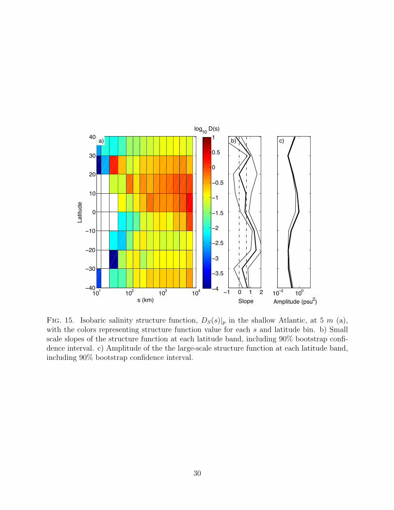
result is that low latitudes show a maximum in isobaric salinity variance near the surface408

(Figures 15), possibly due to fast planetary waves propagating through a highly stratified409

upper ocean, and minima at mid-latitudes, which may characterize the quieter interior of410

subtropical gyres. This behavior is qualitatively, and significantly, different from the case of411

1000 m and the two isopycnal cases (Figures 12-13-14). Comparisons between these surface412

data (Figures 14 & 15) and tow-yos or the Pirata array would be interesting, but there are413

no comparable data to compare to the deep Argo data (Figures 12 & 13)414

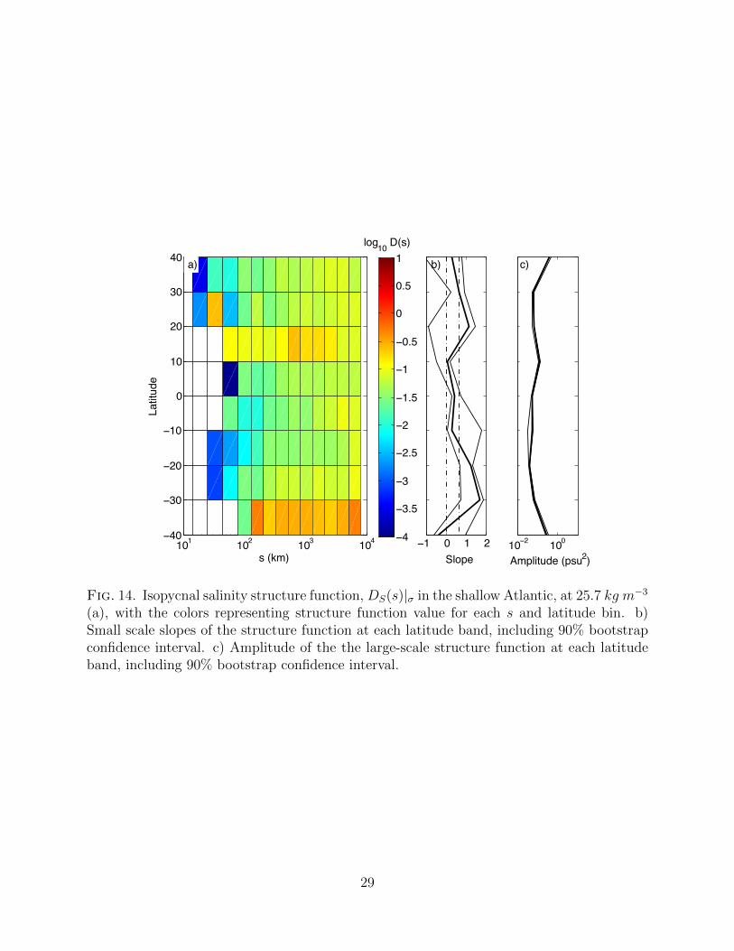
At most latitudes, structure functions in Figures 12-13-14-15 show positive slopes, with415

90% confidence and bootstrap-estimated means that are often near 23. Thus, the proposition416

that this behavior is near-universal is further supported by Figures 12-13-14-15. It is unclear417

whether the one counter-example seen in Fig. 12 is of physical origin or an artifact of the still-418

limited data collection. Bootstrap mean slopes show signs of meridional asymmetry – hints419

25

101 102 103 10410−4

10−3

10−2

10−1

100

s (km)

D S(s) (

psu2 )

a)

101 102 103 10410−4

10−3

10−2

10−1

100

s (km)

D S(s) (

psu2 )

b)

Fig. 11. Isobaric salinity structure function, DS(s)|p, in the a) North (30-40N) and b)South (30-40S, right) Atlantic (red) and Pacific (blue) Oceans at 5 (solid) and 1000 (dashed)meters. Reference slopes of γ = 0 (dashed) and 2

3(solid) are shown in bold.

of slightly steeper slopes in the Northern Hemisphere, and maybe of tropical slope minima.420

However, these slope differences are small and far from being statistically significant, which421

again leads to the conclusion that further accumulation of Argo data is needed to challenge422

the proposed null hypothesis.423

4. Conclusions424

This first application of structure function techniques to Argo data gives physically mean-425

ingful results. 90% confidence intervals estimated by bootstrapping show that there is both426

regional and depth dependence of the structure functions. The majority of the estimates427

discussed here have a slope near 23

on average (the equivalent of a k−5/3 tracer spectrum) in428

an inertial range between 10 and 100 km that varies with location, and slope shows little429

dependence on depth. Many aspects of the method should be re-evaluated (homogeneity,430

isotropy, simultaneity, noise handling, potential biases, mean handling, etc) but a map of431

slopes from Argo, as is done for sea surface height spectra in Xu and Fu (2012), will be432

possible in the near future. Unlike Xu and Fu, the Argo-based map will vary with depth as433

26

101 102 103 104

−30

−20

−10

0

10

20

30

s (km)

Latit

ude

log10 D(s)

−5

−4.5

−4

−3.5

−3

−2.5

−2

−1.5

−1

−2 0 2Slope (psu2 km−1)

10−4 10−2 100

−30

−20

−10

0

10

20

30

Amplitude (psu2)

a) b) c)

Slope

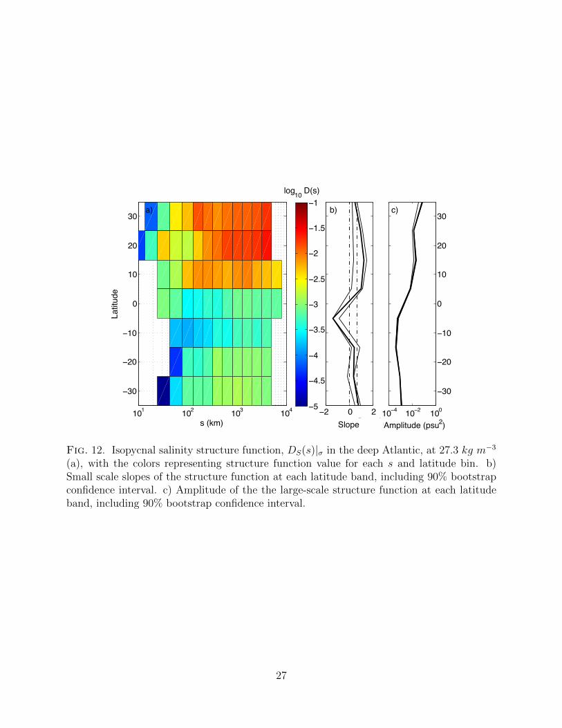
Fig. 12. Isopycnal salinity structure function, DS(s)|σ in the deep Atlantic, at 27.3 kg m−3

(a), with the colors representing structure function value for each s and latitude bin. b)Small scale slopes of the structure function at each latitude band, including 90% bootstrapconfidence interval. c) Amplitude of the the large-scale structure function at each latitudeband, including 90% bootstrap confidence interval.

27

101 102 103 104

−30

−20

−10

0

10

20

30

s (km)

Latit

ude

log10 D(s)

−5

−4.5

−4

−3.5

−3

−2.5

−2

−1.5

−1

0 1 2Slope (psu2 km−1)

10−4 10−2 100

−30

−20

−10

0

10

20

30

Latit

ude

Amplitude (psu2)

a) b) c)

Slope

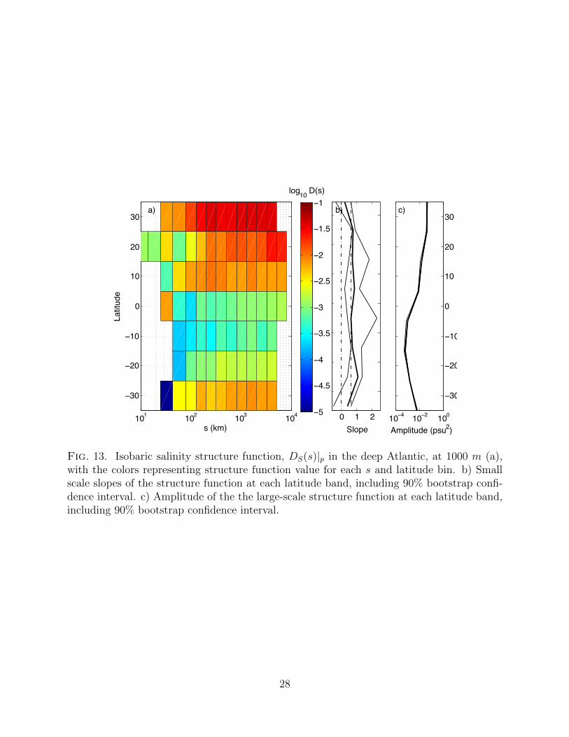
Fig. 13. Isobaric salinity structure function, DS(s)|p in the deep Atlantic, at 1000 m (a),with the colors representing structure function value for each s and latitude bin. b) Smallscale slopes of the structure function at each latitude band, including 90% bootstrap confi-dence interval. c) Amplitude of the the large-scale structure function at each latitude band,including 90% bootstrap confidence interval.

28

101 102 103 104−40

−30

−20

−10

0

10

20

30

40

s (km)

Latit

ude

log10 D(s)

−4

−3.5

−3

−2.5

−2

−1.5

−1

−0.5

0

0.5

1

−1 0 1 2Slope (psu2 km−1)

10−2 100

Amplitude (psu2)

a) b) c)

Slope

Fig. 14. Isopycnal salinity structure function, DS(s)|σ in the shallow Atlantic, at 25.7 kg m−3

(a), with the colors representing structure function value for each s and latitude bin. b)Small scale slopes of the structure function at each latitude band, including 90% bootstrapconfidence interval. c) Amplitude of the the large-scale structure function at each latitudeband, including 90% bootstrap confidence interval.

29

101 102 103 104−40

−30

−20

−10

0

10

20

30

40

s (km)

Latit

ude

log10 D(s)

−4

−3.5

−3

−2.5

−2

−1.5

−1

−0.5

0

0.5

1

−1 0 1 2Slope (psu2 km−1)

10−2 100

Amplitude (psu2)

a) b) c)

Slope

Fig. 15. Isobaric salinity structure function, DS(s)|p in the shallow Atlantic, at 5 m (a),with the colors representing structure function value for each s and latitude bin. b) Smallscale slopes of the structure function at each latitude band, including 90% bootstrap confi-dence interval. c) Amplitude of the the large-scale structure function at each latitude band,including 90% bootstrap confidence interval.

30

the estimates do here (Figures 12-13-14-15). This work provides a first step in that direction.434

The scale of the bend point–if it indeed signifies the largest scale of coherent variability–is435

also a potentially useful measure. Estimates of eddy scales (e.g., Tulloch et al. 2011) rarely436

use in situ data, as the data volume required is enormous. These scales can be read off of the437

left panels of Figures 12-13-14-15 as the s value for each latitude where all larger values are438

of similar magnitude. Roughly, this scale is 100 km, but latitudinal and depth variations are439

indicated (although noisily). The structure function of Argo offers a potentially inexpensive440

estimate of these scales.441

Finally, it is possible, or even likely, that sampling biases are inherent in the style of442

sampling based on Lagrangian float technology. That is, floats will be unlikely to drift into443

or out of coherent structures, and are likely to be ejected from regions of high eddy activity444

toward lower energy regions (e.g., Davis 1991). Without a substantially higher density of445

observations, such biases due to sampling heterogeneity are not easily detected generically446

and so are neglected here. However, all structure functions result from a large number447

of observational pairs (see Appendix B), and instrument error analysis and bootstrapping448

confidence intervals are used to verify these assumptions (see Appendices B and C). A com-449

parison between the Argo structure functions and those from stationary Eulerian moorings,450

e.g., TAO/TRITON, RAMA, and PIRATA, would help quantify such biases.451

Neither structure function nor spectral slope is a conclusive proof of any particular be-452

havior, but they are very useful in eliminating theories or models that are erroneous. Even453

with discontinuous and spotty temperature or salinity measurements, an appreciation of the454

turbulence statistics at greater depths and over broader geographic regions than previously455

observed is now possible, and will only improve with the growth of the Argo dataset. The456

ability to infer a spectrum from a structure function, even in a case where two distinct struc-457

ture function slopes are present and data is filled with gaps is suited to Argo data analyses.458

The primary limitation is data density, as spatial refinement reduces the amount of obser-459

vation pairs that can be used. As more Argo data become available, the noisiness in the460

31

structure functions can be smoothed, the limiting velocity, cmax can be increased to include461

more pairs with smaller separation times, and bootstrap intervals can be narrowed.462

This work has opened many possibilities for future studies beyond the results already463

presented. Alongside the increasing number of Argo floats measuring at depth, it would be464

beneficial to include other sources of data (e.g., mooring data) to fill in the spatial gaps465

in Argo’s network that would allow the structure function to be calculated further into466

the inertial range of the oceans at smaller scales. Adding a method for estimating the467

velocity and velocity-tracer covariances would greatly enhance the dynamical detail possible468

from structure function analysis. This method can also be extended to scattered velocity469

observations in order to directly measure the kinetic energy structure function.470

Acknowledgments.471

This paper was inspired by conversations with Rod Frehlich. We wish that there had472

been more time with Rod, so that we could learn more from him. The Argo Program is part473

of the Global Ocean Observing System. KM was supported by the CIRES/NOAA-ESRL474

Graduate Research Fellowship. BF-K was supported by NSF 0855010 and 1245944 and GF475

was supported in part through NASA project “Estimating the Circulation and Climate of476

the Ocean (ECCO) for CLIVAR” and NSF 1023499.477

32

APPENDIX A478

479

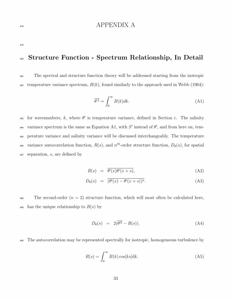
Structure Function - Spectrum Relationship, In Detail480

The spectral and structure function theory will be addressed starting from the isotropic481

temperature variance spectrum, B(k), found similarly to the approach used in Webb (1964):482

θ′2 =

∫ ∞0

B(k)dk. (A1)

for wavenumbers, k, where θ′ is temperature variance, defined in Section c. The salinity483

variance spectrum is the same as Equation A1, with S ′ instead of θ′, and from here on, tem-484

perature variance and salinity variance will be discussed interchangeably. The temperature485

variance autocorrelation function, R(s), and nth-order structure function, Dθ(s), for spatial486

separation, s, are defined by487

R(s) = θ′(x)θ′(x+ s), (A2)

Dθ(s) = (θ′(x)− θ′(x+ s))n. (A3)

The second-order (n = 2) structure function, which will most often be calculated here,488

has the unique relationship to R(s) by489

Dθ(s) = 2(θ′2 −R(s)). (A4)

The autocorrelation may be represented spectrally for isotropic, homogeneous turbulence by490

R(s) =

∫ ∞0

B(k) cos[ks]dk. (A5)

33

Using the relationship between the autocorrelation and structure function from (A4), and491

the spectral definition of autocorrelation in (A5), the structure function can be written492

spectrally by493

Dθ(s) = 2

∫ ∞0

B(k) (1− cos[ks]) dk. (A6)

As mentioned in Section a, for a given spectrum, B(k) = αBkλ, with a single spectral slope,494

λ, over a range from kmin < k < kmax and a given structure function, Dθ(s) = αDsγ, with a495

single structure function slope, γ, a change of variables (ks→ ξ) yields496

Dθ(s) = 2

∫ ∞0

αBkλ (1− cos[ks]) dk

= 2αBs−λ−1

∫ ∞0

ξλ (1− cos ξ) dξ

= sγ[2αB

∫ ∞0

ξλ (1− cos ξ) dξ]. (A7)

This shows that γ = −λ− 1, relating the slope of the structure function, γ, to the spectral497

slope, λ. Webb (1964) shows that outside of the inertial range [kmin, kmax], the contribution498

to the spectrum is small, so (A7) can be truncated and written as499

Dθ(s) = sγ[2αB

∫ kmaxs

kmins

ξλ (1− cos ξ) dξ]. (A8)

One could make the same argument for the kinetic energy spectrum, E(k), and velocity500

structure function, DU(s). Thus,501

U2 =

∫ ∞0

E(k)dk (A9)

DU(s) = (u(x)− u(x+ s))2. (A10)

Following the same method, DU(s) ∝ sβD and E(k) ∝ kβE produce the same relationship:502

βD = −βE − 1.503

34

In the case of a tracer variance spectrum with a direct and indirect cascade producing504

two power-law scalings (as is the case in Nastrom and Gage (1985)), (A6) can be split into505

four pieces spanning intervals in k:506

Dθ(s) = 2

∫ ∞0

B(k) (1− cos[ks]) dk

= 2

(∫ kmin

0

B(k) (1− cos[ks]) dk +

∫ k1

kmin

α1kλ1 (1− cos[ks]) dk

)+

2

(∫ kmax

k1

α2kλ2 (1− cos[ks]) dk +

∫ ∞kmax

B(k) (1− cos[ks]) dk

). (A11)

Since the first and the last integrals are definite and negligible (Webb 1964), inserting507

the continuity of B(k) (α1kλ11 = α2k

λ21 ) produces508

Dθ(s) = 2α1

(∫ k1

kmin

kλ1 (1− cos[ks]) dk + kλ1−λ21

∫ kmax

k1

kλ2 (1− cos[ks]) dk

)(A12)

Assuming each of the two inertial ranges is large (kmin << k1 << kmax) the structure509

function is dominated by only one of the two integrals in (A12), depending on scale of s510

when compared with the wavenumber (kmin < 1/s < k1 or k1 < 1/s < kmax). Performing511

the change of variables as done above for the single power law case, gives the structure512

function in terms of s,513

Dθ(s) = 2

(α1s

−λ1−1∫ k1s

kmins

ξλ1 (1− cos[ξ]) dξ + α2s−λ2−1

∫ kmaxs

k1s

ξλ2 (1− cos[ξ]) dξ

).

(A13)

Thus, when the inertial ranges are deep, the structure function is closely approximated by514

a polynomial with two terms:515

Dθ(s) = c1sγ1 + c2s

γ2 , (A14)

with γ1 = −λ2−1 and γ2 = −λ1−1, and an internal dependence on s that determines which516

term dominates the spectrum. The analysis of Nastrom and Gage (1985) confirmed that the517

bend point where the structure function switches from being dominated by the second to the518

35

first term happens near s ∼ 1/k1, although this result was much clearer when the inertial519

ranges were made wider than those in the actual observations of Nastrom and Gage (1985).520

Other prototypical dual cascade spectra were also tested, yielding similar results (e.g., the521

direct and indirect cascades of 2D turbulence from Kraichnan 1967).522

36

APPENDIX B523

524

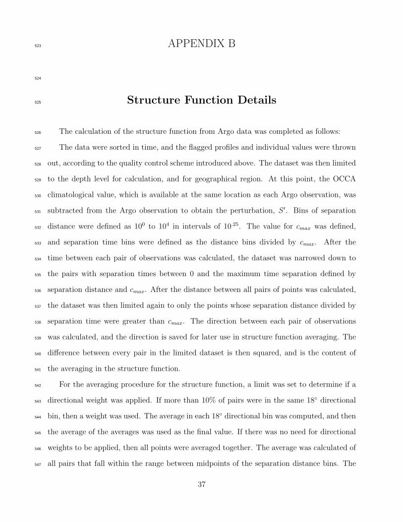
Structure Function Details525

The calculation of the structure function from Argo data was completed as follows:526

The data were sorted in time, and the flagged profiles and individual values were thrown527

out, according to the quality control scheme introduced above. The dataset was then limited528

to the depth level for calculation, and for geographical region. At this point, the OCCA529

climatological value, which is available at the same location as each Argo observation, was530

subtracted from the Argo observation to obtain the perturbation, S ′. Bins of separation531

distance were defined as 100 to 104 in intervals of 10.25. The value for cmax was defined,532

and separation time bins were defined as the distance bins divided by cmax. After the533

time between each pair of observations was calculated, the dataset was narrowed down to534

the pairs with separation times between 0 and the maximum time separation defined by535

separation distance and cmax. After the distance between all pairs of points was calculated,536

the dataset was then limited again to only the points whose separation distance divided by537

separation time were greater than cmax. The direction between each pair of observations538

was calculated, and the direction is saved for later use in structure function averaging. The539

difference between every pair in the limited dataset is then squared, and is the content of540

the averaging in the structure function.541

For the averaging procedure for the structure function, a limit was set to determine if a542

directional weight was applied. If more than 10% of pairs were in the same 18◦ directional543

bin, then a weight was used. The average in each 18◦ directional bin was computed, and then544

the average of the averages was used as the final value. If there was no need for directional545

weights to be applied, then all points were averaged together. The average was calculated of546

all pairs that fall within the range between midpoints of the separation distance bins. The547

37

Region # of profiles # of pairs

10S-10N, 180W-150W 14236 109873410S-Eq, 180-165W 3537 2919410S-Eq, 165-150W 3758 39664Eq-10N, 180-165W 3484 32588Eq-10N, 165-150W 3456 32509

Table 2. Number of profiles and pairs used to compute the structure function in theheterogeneous region analysis in Figure 4.

values that contributed to each separation distance’s bin were saved for calculation of the548

confidence intervals, which will be discussed below.549

The tables included here show the details of the structure function calculations; Tables 2550

& 4 list the numbers of float profiles in each calculation and the number of “simultaneous”551

pairs used, and Tables 3 & 5 list the 95% bootstrap confidence intervals for the structure552

functions.553

The 95% bootstrap confidence interval was calculated because the population of pairs554

that contribute to the average in the structure function are not normally distributed, so the555

standard deviation of the observations is not sufficient. Using the Central Limit Theorem556

(Devore 2009), which states that the means, xn from n samples of a population (here, the557

pairs of simultaneous observations), are normally distributed, and therefore, the population558

mean (µ, the true quantity of the structure function) is the mean of the sample means559

(µ = xn). Therefore, the confidence interval is the area with a 95% probability that it560

contains the true structure function value. This theorem is only true when n is sufficiently561

large (usually larger than n = 30, though some populations may require more), so n = 200562

was used here.563

Kuroshio homogeneous region, “uniform” at 5 m:564

SW: lon = 141; lat= 33;565

NW: lon = 142; lat= 43;566

SE: lon = 155; lat= 42;567

38

Region 10S-10N, 10S-Eq, 10S-Eq, Eq-10N,W Eq-10N,180W-150W 180-165W 165-150W 180-165W 165-150W

s (103 km)

0.0139 2.3±0.3069 NaN NaN NaN 0.9±0.30680.0247 1.6±0.1153 NaN NaN NaN 0.7±0.08460.0439 3.4± 0.1492 7.2±0.4158 0.5±0.0203 5.8±0.3515 4.7±0.27220.0781 9.3±0.2352 11.7±0.9514 8.1±0.2947 13.4±0.6854 9.5±0.48170.1292 25.4±0.2157 31.5±0.6355 10.4±0.1810 31.1±0.6352 26.6±0.40080.2048 30.4±0.1330 31.9±0.2762 15.4±0.1035 61.4±0.4863 30.3±0.31920.3246 42.7±0.1127 35.2±0.2894 29.1±0.1250 83.0±0.4407 51.6±0.27030.5145 54.5±0.0728 65.2±0.1959 31.7±0.0779 104.8±0.2505 71.5±0.19700.8155 66.9±0.0393 71.7±0.1704 46.2±0.0550 85.9±0.1561 74.0±0.12901.2924 73.7±0.0266 94.6±0.1830 51.3±0.0645 88.5±0.1539 67.8±0.10372.0484 90.5±0.0252 99.3±0.6636 62.2±0.2756 65.7±0.4382 70.6±0.37113.2465 105.8±0.0426 NaN NaN NaN NaN

Table 3. The structure function plus/minus the 95% bootstrap confidence interval for thestructure function in the heterogeneous region analysis in Figure 4. All values are 10−3 psu2.

Depth # of profiles # of pairs

25.5 3649 3422826.1 4549 6054626.4 4620 6525126.6 4608 6589426.8 4668 6641727.0 4768 6793027.2 4764 67848

Table 4. Number of profiles and pairs used to compute the structure function in Figure 3.

NE: lon = 157; lat= 42;568

Heterogeneous region, “non-uniform” at 25.9kg m−3 and 5 m:569

SW: lon = -160; lat= 10;570

NW: lon = -160; lat= 30;571

SE: lon = -140; lat= 10;572

NE: lon = -140; lat= 30;573

39

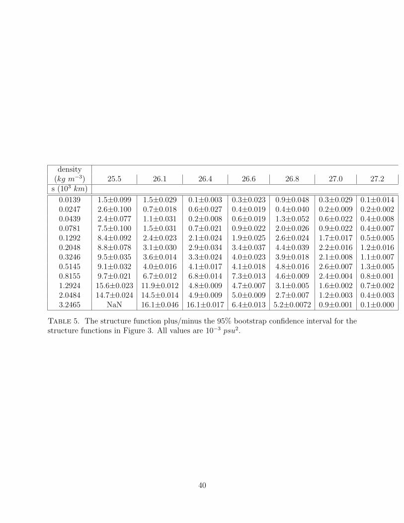
density(kg m−3) 25.5 26.1 26.4 26.6 26.8 27.0 27.2

s (103 km)

0.0139 1.5±0.099 1.5±0.029 0.1±0.003 0.3±0.023 0.9±0.048 0.3±0.029 0.1±0.0140.0247 2.6±0.100 0.7±0.018 0.6±0.027 0.4±0.019 0.4±0.040 0.2±0.009 0.2±0.0020.0439 2.4±0.077 1.1±0.031 0.2±0.008 0.6±0.019 1.3±0.052 0.6±0.022 0.4±0.0080.0781 7.5±0.100 1.5±0.031 0.7±0.021 0.9±0.022 2.0±0.026 0.9±0.022 0.4±0.0070.1292 8.4±0.092 2.4±0.023 2.1±0.024 1.9±0.025 2.6±0.024 1.7±0.017 0.5±0.0050.2048 8.8±0.078 3.1±0.030 2.9±0.034 3.4±0.037 4.4±0.039 2.2±0.016 1.2±0.0160.3246 9.5±0.035 3.6±0.014 3.3±0.024 4.0±0.023 3.9±0.018 2.1±0.008 1.1±0.0070.5145 9.1±0.032 4.0±0.016 4.1±0.017 4.1±0.018 4.8±0.016 2.6±0.007 1.3±0.0050.8155 9.7±0.021 6.7±0.012 6.8±0.014 7.3±0.013 4.6±0.009 2.4±0.004 0.8±0.0011.2924 15.6±0.023 11.9±0.012 4.8±0.009 4.7±0.007 3.1±0.005 1.6±0.002 0.7±0.0022.0484 14.7±0.024 14.5±0.014 4.9±0.009 5.0±0.009 2.7±0.007 1.2±0.003 0.4±0.0033.2465 NaN 16.1±0.046 16.1±0.017 6.4±0.013 5.2±0.0072 0.9±0.001 0.1±0.000

Table 5. The structure function plus/minus the 95% bootstrap confidence interval for thestructure functions in Figure 3. All values are 10−3 psu2.

40

Depth No. profiles No. pairs Depth No. profiles No. pairs

5m 3927 19383 360m 5665 4303415m 5747 51574 380m 5743 4432025m 6209 62357 400m 5561 4253135m 6292 62408 420m 4378 2660545m 5966 61334 440m 4589 3162755m 6278 61816 460m 5200 3948865m 6208 61002 480m 5182 3797175m 6017 58401 500m 5370 4138685m 6111 56751 550m 5381 4120495m 6110 54444 600m 5365 40905105m 5532 45353 650m 5119 36565115m 5806 44674 700m 5257 39031125m 5592 42608 750m 5096 36193135m 5611 44095 800m 5304 39631145m 5590 42647 850m 5020 35310155m 5834 44958 900m 5260 39069165m 5380 41946 950m 4937 34395175m 5802 44475 1000m 4917 36343185m 5577 42378 1100m 4796 34845200m 5838 45174 1200m 4627 32091220m 5840 45391 1300m 4551 31028240m 5840 45135 1400m 3573 22269260m 5712 43950 1500m 3428 20762280m 5783 44871 1600m 3319 20461300m 5014 31869 1700m 3270 20042320m 5704 43439 1800m 3187 19231340m 5828 44912 1900m 2831 14045

Table 6. Number of profiles and profile pairs used to compute the isobaric structure functionfor each depth in the “uniform” region of the Kuroshio, shown in Figure 9.

41

Depth No. profiles No. pairs Depth No. profiles No. pairs

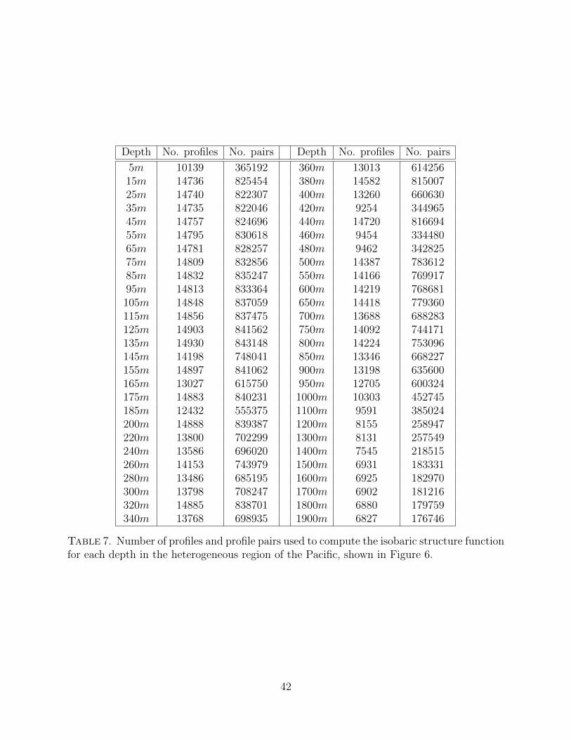
5m 10139 365192 360m 13013 61425615m 14736 825454 380m 14582 81500725m 14740 822307 400m 13260 66063035m 14735 822046 420m 9254 34496545m 14757 824696 440m 14720 81669455m 14795 830618 460m 9454 33448065m 14781 828257 480m 9462 34282575m 14809 832856 500m 14387 78361285m 14832 835247 550m 14166 76991795m 14813 833364 600m 14219 768681105m 14848 837059 650m 14418 779360115m 14856 837475 700m 13688 688283125m 14903 841562 750m 14092 744171135m 14930 843148 800m 14224 753096145m 14198 748041 850m 13346 668227155m 14897 841062 900m 13198 635600165m 13027 615750 950m 12705 600324175m 14883 840231 1000m 10303 452745185m 12432 555375 1100m 9591 385024200m 14888 839387 1200m 8155 258947220m 13800 702299 1300m 8131 257549240m 13586 696020 1400m 7545 218515260m 14153 743979 1500m 6931 183331280m 13486 685195 1600m 6925 182970300m 13798 708247 1700m 6902 181216320m 14885 838701 1800m 6880 179759340m 13768 698935 1900m 6827 176746

Table 7. Number of profiles and profile pairs used to compute the isobaric structure functionfor each depth in the heterogeneous region of the Pacific, shown in Figure 6.

42

Density No. profiles No. pairs Density No. profiles No. pairs

24.9kgm−3 11652 483239 26.4kgm−3 13841 73691725.0kgm−3 11997 512881 26.5kgm−3 13928 73910125.1kgm−3 11823 496640 26.6kgm−3 13956 74143325.2kgm−3 11483 470120 26.7kgm−3 14043 74868725.3kgm−3 11034 425446 26.8kgm−3 14169 76102525.4kgm−3 10927 424389 26.9kgm−3 14373 78229125.5kgm−3 10987 427971 27.0kgm−3 14340 77176625.6kgm−3 11129 443197 27.1kgm−3 14320 76762125.7kgm−3 11547 480032 27.2kgm−3 14358 77287825.8kgm−3 11680 488667 27.3kgm−3 14287 76554025.9kgm−3 12160 538459 27.4kgm−3 10154 43928526.0kgm−3 12490 571559 27.5kgm−3 8155 25951026.1kgm−3 13101 637287 27.6kgm−3 6932 18370126.2kgm−3 13621 700790 27.7kgm−3 26 326.3kgm−3 13905 733375

Table 8. Number of profiles and profile pairs used to compute the isopycnal structurefunction for each density level in the heterogeneous region of the Pacific, shown in Figure 7.

43

APPENDIX C574

575

Error Analysis576

An important aspect of structure function analysis that must be included is an under-577

standing of random noise. Lester et al. (1970) showed that the structure function of Gaussian578

white noise has a slope of γ = 0, so those results were replicated with a randomly generated579

dataset of temperatures and salinities with changing standard deviations. The same calcu-580

lation was particularly important to determine the noise level generated by measurement581

error. Using the square of the known standard error of the Argo measurements of temper-582

ature and salinity (.01 degree Celsius and .01 psu, respectively) as the standard deviation,583

and a typical temperature and salinity value for the mean, a Gaussian dataset was created,584

and the structure function was calculated. A noise floor for the structure function includ-585

ing the error from the climatology was also considered, using the total standard deviation,586

σtot =√σ2Argo + σ2

clim. This more realistic noise floor of O(10−4) is still below the majority587

of the structure functions calculated, allowing this analysis of turbulence from Argo data to588

continue without fear of data measurement errors interfering.589

44

APPENDIX D590

591

Line-Fitting Algorithm592

In order to quantify the differences among structure functions, a line-fitting algorithm593

was created to extract the slopes of the structure functions with one (or two) linear fit(s).594

A test was first performed to decide whether more than one linear fit was needed. On595

the structure functions with only one slope, a least-squares method of linear regression was596

performed, using the bootstrap method of sampling to obtain a confidence interval. The597

advantage of using the bootstrap method for the confidence interval is that the assumption598

of normality for the individual observations is not necessary.599

Since the relationship to the spectral slope no longer holds in heterogeneous regions,600

there could be two separate linear slope regimes with no relation to the spectrum. In this601

case, the same linear regression was performed, but in steps so as to find the amplitude and602

approximate bend point where a change in slope occurs. A bootstrap analysis was completed603

for this process. First, randomly chosen data points were fitted by two lines with the bend604

point at each separation distance bin. A least-squares error was calculated for the lines fit605

for each bend point, and the bend point with the smallest error was chosen (sbend). Using606

that bend point, all data points were then considered for the best-fit line. Another bootstrap607

regime was then run, choosing random data points and calculating the resulting slopes of the608

best-fit lines for the sub-sets of the original data. A bootstrap interval using 200 subsamples609

was calculated from these results, providing a confidence interval for the chosen best fit from610

all points. The amplitudes discussed are determined as the average of the points above the611

bend point.612

The resulting bend points were not presented here because the changes in bend point613

between structure functions were small compared to the confidence intervals. With the614

45

addition of more data, and subsequently less-noisy structure functions, this metric can also615

be used to quantify the bend point, which is the largest eddy scale measured.616

In the homogeneous regions where two structure function slopes are discerned, the same617

linear fitting regime was used, and the relation to the spectral slope was applied to the618

results. The bend point for the spectral slope could then computed to be k1 = 1/sbend.619

46

620

REFERENCES621

Argo Science Team, 1998: On the design and implementation of argo. International CLIVAR622

Project Office Rep. 21, GODAE Rep. 5.623

Batchelor, G. K., 1959: Small-scale variation of convected quantities like temperature in624

turbulent fluid .1. General discussion and the case of small conductivity. Journal of Fluid625

Mechanics, 5 (1), 113–133.626

Bennett, A., 1984: Relative dispersion: Local and nonlocal dynamics. Journal of the atmo-627

spheric sciences, 41 (11), 1881–1886.628

Blumen, W., 1978: Uniform potential vorticity flow .1. Theory of wave interactions and629

2-dimensional turbulence. Journal of the Atmospheric Sciences, 35 (5), 774–783.630

Buhler, O., J. Callies, and R. Ferrari, 2014: Wave-vortex decomposition of one-dimensional631

ship-track data. Journal of Fluid Mechanics, 756, 1007–1026.632

Callies, J. and R. Ferrari, 2013: Interpreting energy and tracer spectra of upper-ocean633

turbulence in the submesoscale range (1-200 km). Journal of Physical Oceanography, in634

press.635

Carval, T., et al., 2011: Argo user’s manual, version 2.31. Tech. rep., Argo Data Management.636

Charney, J. G., 1971: Geostrophic turbulence. Journal of the Atmospheric Sciences, 28,637

1087–1095.638

Chelton, D. B., R. A. Deszoeke, M. G. Schlax, K. El Naggar, and N. Siwertz, 1998: Geo-639

graphical variability of the first baroclinic rossby radius of deformation. Journal of Physical640

Oceanography, 28 (3), 433–460.641

47

Cole, S. and D. Rudnick, 2012: The spatial distribution and annual cycle of upper ocean642

thermohaline structure. Journal of Geophysical Research-Oceans, 117.643

Corrsin, S., 1951: On the spectrum of isotropic temperature fluctuations in isotropic turbu-644

lence. Journal of Applied Physics, 22 (469).645

Davis, R. E., 1991: Lagrangian ocean studies. Annual Review of Fluid Mechanics, 23 (1),646

43–64.647

Devore, J., 2009: Probability and Statistics for Engineering and the Scientes, Seventh Edi-648

tion. Brooks/Cole, Belmont, CA.649

Forget, G., 2010: Mapping ocean observations in a dynamical framework: A 2004-06 ocean650

atlas. Journal of Physical Oceanography, 40, 1201–1221.651

Forget, G. and C. Wunsch, 2007: Estimated global hydrographic variability. Journal of652

Physical Oceanography, 37 (8), 1997–2008, doi:DOI10.1175/JPO3072.1.653

Fox-Kemper, B., et al., 2011: Parameterization of mixed layer eddies. III: Implementation654

and impact in global ocean climate simulations. Ocean Modelling, 39, 61–78, doi:10.1016/655

j.ocemod.2010.09.002, URL http://dx.doi.org/10.1016/j.ocemod.2010.09.002.656

Frehlich, R. and R. Sharman, 2004: Estimates of turbulence from numerical weather pre-657

diction model output with applications to turbulence diagnosis and data assimilation.658

Monthly Weather Review, 132, 2308–2324.659

Frehlich, R. and R. Sharman, 2010: Climatology of velocity and temperature turbulence660

statistics determined from rawinsonde and ACARS/AMDAR data. Journal of Applied661

Meteorology and Climatology, 49 (6), 1149–1169.662

Garrett, C. and W. Munk, 1972: Space-time scales of internal waves. Geophysical Fluid663

Dynamics, 2, 225–264.664

48

Hamilton, K., Y. O. Takahashi, and W. Ohfuchi, 2008: Mesoscale spectrum of atmospheric665

motions investigated in a very fine resolution global general circulation model. Journal of666

Geophysical Research, 118.667

Hosegood, P., M. C. Gregg, and M. H. Alford, 2006: Sub-mesoscale lateral density struc-668

ture in the oceanic surface mixed layer. Geophysical Research Letters, 33 (L22604),669

doi:10.1029/2006GL026 797.670

Klein, P., A. M. Treguier, and B. L. Hua, 1998: Three-dimensional stirring of thermohaline671

fronts. Journal of Marine Research, 56 (3), 589–612.672

Klymak, J. M. and J. N. Moum, 2007: Oceanic isopycnal slope spectra. part i: Internal673

waves. Journal of physical oceanography, 37 (5), 1215–1231.674

Kolmogorov, A. N., 1941: The local structure of turbulence in incrompressible viscous fluid675

for very large reynolds number. Dokl. Akad. Nauk. SSSR, 30, 9–13.676

Koshyk, J. N. and K. Hamilton, 2001: The horizontal kinetic energy spectrum and spectral677

budget simulated by a high-resolution troposphere-stratosphere mesosphere gcm. Journal678

of Atmospheric Sciences, 58, 329–348.679

Kraichnan, R. H., 1967: Inertial ranges in two-dimensional turbulence. Physics of Fluids,680

16, 1417–1423.681

Kraichnan, R. H., 1994: Anomalous scaling of a randomly advected passive scalar. Physical682

review letters, 72 (7), 1016.683

Kunze, E., 1985: Near-inertial wave propagation in geostrophic shear. Journal of Physical684

Oceanography, 15 (5), 544–565.685

Lester, P., E. Reiter, and C. S. U. D. of Atmospheric Science, 1970: The Application of Shear686

Functions in the Study of the Meso- and Microstructure of the Atmosphere. Atmospheric687

49

science paper, Department of Atmospheric Science, Colorado State University, URL http:688

//books.google.com/books?id=F\_nVSgAACAAJ.689

Lindborg, E., 1999: Can the atmospheric kinetic energy spectrum be explained by two-690

dimensional turbulence? Journal of Fluid Mechanics, 388, 259–288.691

Millero, F. J., R. Feistel, D. G. Wright, and T. J. McDougall, 2008: The composition of692

standard seawater and the definition of the reference-composition salinity scale. Deep Sea693

Research Part I: Oceanographic Research Papers, 55 (1), 50–72.694

Nastrom, G. D. and K. S. Gage, 1985: A climatology of atmospheric wavenumber spectra695

of wind and temperature observed by commercial aircraft. Journal of the Atmospheric696

Sciences, 42, 950–960.697

Obukhov, A. M., 1949: The structure of the temperature field in a turbulent flow. Izv. Akad.698

Nauk. SSSR, Ser. Geog. and Geophys., 13 (58).699

Pierrehumbert, R., 1994: Tracer microstructure in the large-eddy dominated regime. Chaos,700

Solitons & Fractals, 4 (6), 1091–1110.701

Roullet, G., X. Capet, and G. Maze, 2014: Global interior eddy available potential energy702

diagnosed from argo floats. Geophysical Research Letters, 41 (5), 1651–1656.703

Rudnick, D. L. and R. Ferrari, 1999: Compensation of horizontal temperature and salinity704

gradients in the ocean mixed layer. Science, 283 (5401), 526–529.705

Salmon, R., 1982: Geostrophic turbulence. Topics in Ocean Physics, A. R. Osborne and706

P. M. Rizzoli, Eds., Proceedings of the International School of Physics Enrico Fermi (July707

1980), Course LXXX.708

Scott, R. B. and F. Wang, 2005: Direct evidence of an oceanic inverse kinetic energy cascade709

from satellite altimetry. Journal of Physical Oceanography, 35, 1650–1666.710

50

She, Z.-S. and E. Leveque, 1994: Universal scaling laws in fully developed turbulence. Phys-711

ical Review Letters, 72, 336–339.712

Skamarock, W. C., 2004: Evaluating mesoscale NWP models using kinetic energy spectra.713

Monthly Weather Review, 132, 3019–3032.714

Takahashi, Y. O., K. Hamilton, and W. Ohfuchi, 2006: Explicit global simulation of the715

mesoscale spectrum of atmospheric motions. Geophysical Research Letters, 33.716

Tulloch, R., J. Marshall, C. Hill, and K. S. Smith, 2011: Scales, growth rates, and spectral717

fluxes of baroclinic instability in the ocean. Journal of Physical Oceanography, 41 (6),718

1057–1076.719

Tulloch, R. and K. S. Smith, 2006: A theory for the atmospheric energy spectrum: Depth-720

limited temperature anomalies at the tropopause. Proceedings of the National Academy of721

Sciences, 103 (40), 14 690 14 694.722

Vallis, G. K., 2006: Atmospheric and Oceanic Fluid Dynamics : Fundamentals and Large-723

Scale Circulation. Cambridge University Press, Cambridge.724

Webb, E. K., 1964: Ratio of spectrum and structure-function constants in the inertial sub-725

range. Quarterly Journal of the Royal Meteorological Society, 90 (385), 344–345.726

Xu, Y. and L.-L. Fu, 2012: The effects of altimeter instrument noise on the estimation of the727

wavenumber spectrum of sea surface height. Journal of Physical Oceanography, 42 (12),728

2229–2233.729

Yaglom, A., 1949: Local structure of the temperature field in a turbulent flow. Doklady730

Akademii Nauk, 69 (6), 743–746.731

Yeager, S. G. and W. G. Large, 2007: Observational evidence of winter spice injection.732

Journal of Physical Oceanography, 37, 2895–2919, doi:DOI10.1175/2007JPO3629.1.733

51