Spatial variability of seabird distribution associated with environmental factors: a case study of marine Important Bird Areas in the Azores

Spatial variability of seabird distribution associated withenvironmental factors: a case study of marine ImportantBird Areas in the Azores

Patrıcia Amorim, Miguel Figueiredo, Miguel Machete, Telmo Morato, Ana Martins,and Ricardo Serrao Santos

Amorim, P., Figueiredo, M., Machete, M., Morato, T., Martins, A., and Serrao Santos, R. 2009. Spatial variability of seabird distribution associatedwith environmental factors: a case study of marine Important Bird Areas in the Azores. – ICES Journal of Marine Science, 66: 29–40.

The spatial structure and distribution at sea of Cory’s shearwaters (Calonectris diomedea borealis), common terns (Sterna hirundo), androseate terns (Sterna dougallii) were analysed in the Azores for various environmental factors: sea surface temperature, chlorophyll aconcentration, distance to fronts, wind, distance to island shore or tern colonies, distance to seamounts, seabed slope, and depth. Dataon seabird sightings were collected by observers on board fishing vessels, 2002 –2006. Generalized linear modelling (GLM) explained 43and 11% of the abundance variability for terns (both species pooled) and Cory’s shearwaters, respectively. Variability in seabird abun-dance was mainly explained by month, wind, distance to shore and/or tern colonies, and distance to seamounts. Variogram modellingindicated that species distribution presented a small-scale spatial structure (i.e. low autocorrelation). Cory’s shearwater predictive dis-tribution maps showed widespread distribution patterns of abundance, despite occurring at a greater intensity around the islands andaround some seamounts, which are areas of fishery interest. Conversely, terns were essentially concentrated near the shore. The estab-lishment of marine important bird areas should be encouraged close to seabird colonies and around some seamount areas.

Keywords: Azores, geostatistics, marine IBAs, regression models, seabirds, spatial statistics.

Received 27 October 2007; accepted 27 May 2008; advance access publication 5 November 2008.

P. Amorim, M. Figueiredo, M. Machete, T. Morato, A. Martins and R. Serrao Santos: IMAR/Azores and Department of Oceanography and Fisheries,University of the Azores, PT- 9901-862 Horta, Portugal. Correspondence to P. Amorim: tel: þ351 292 200 400; fax: þ351 292 200 411; e-mail:[email protected].

IntroductionIt is widely recognized that species distribution varies over space andtime as a result of the selection of preferred habitat and environ-mental conditions (e.g. Ballance et al., 2006). The influence ofenvironmental factors in the at-sea spatial distribution of seabirdshas been widely investigated, although most studies have focusedon productive continental shelves in subpolar and coastal upwellingsystems (see reviews by Hunt and Schneider, 1987; Hunt et al., 1999).Yet, considerably less is known about the habitats of oceanic birds insubtropical and tropical waters, especially in the oceanic realm (for areview, see Ballance and Pitman, 1999). The most common par-ameters used to explain spatial seabird distribution are water masstypes quantified through sea surface temperature (SST) and salinitymeasurements (Ainley et al., 2005; Hyrenbach et al., 2007), oceanproductivity indexed using the concentration of chlorophyll a (Chla) as a proxy (e.g. Louzao et al., 2006; Yen et al., 2006), windspeed(e.g. Spear and Ainley, 1998; Suryan et al., 2006), mesoscale featuresincluding eddies (e.g. Hyrenbach et al., 2006; Yen et al., 2006) andtemperature–salinity fronts (e.g. Begg and Reid, 1997; Ainley et al.,2005), topographic features (e.g. Schneider, 1997; Yen et al., 2004;Morato et al., 2008a), and distance to colonies (e.g. Garthe, 1997;Hyrenbach et al., 2007).

The Azores Archipelago is located in the subtropical NortheastAtlantic, and it represents an ornithological transition between the

tropical and temperate waters (Monteiro et al., 1996a). Cory’sshearwater (Calonectris diomedea borealis) is the most abundantseabird in the area (Table 1), representing the largest concentrationof the subspecies borealis in the world (Monteiro, 2000; BirdLifeInternational, 2004). The common tern (Sterna hirundo) alsooccurs very frequently in the Azores (Table 1), whereas the popu-lation of the roseate tern (Sterna dougallii) in the Azores is esti-mated to be the largest in Europe (Santos et al., 1995; Monteiro,2000). The global conservation status of these species is of “leastconcern” (BirdLife International). However, at the Europeanlevel, the three species are listed in Annex I of the EC BirdsDirective, i.e. are considered of conservation concern. The mainthreats that affect shearwaters and terns in the Azores are relatedto predation (rats, gulls, etc.), anthropogenic disturbance, changesin vegetation, habitat damage by herbivores, and potential compe-tition for food resources with fisheries (Monteiro et al., 1996a).

Seabird conservation is well advanced in the Azores, where 13special protection areas (SPAs) have been designated under theEC Birds Directive. However, these are terrestrial SPAs and there-fore do not encompass any of the critical coastal and offshorewaters such as at-sea feeding or resting areas. Because the Azoresarchipelago is an important breeding area, chiefly for Cory’sshearwaters, proactive measures are necessary to protect theseimportant ecological resources. In particular, information on the

# 2008 International Council for the Exploration of the Sea. Published by Oxford Journals. All rights reserved.For Permissions, please email: [email protected]

29

critical habitats where these seabirds forage and interact with fish-eries is essential to identify and delineate potential protected areas.

The main objective of this study is to analyse potential relation-ships between the spatial structure and distribution of the threeseabird species breeding in the Azores (Cory’s shearwater and twospecies of tern) and environmental factors, taking into account sea-sonal variability along with the development of predictive habitatmodels. This study is the first that incorporates geostatisticalmethods. This information will be applied to the identificationand delineation of marine Important Bird Areas (IBAs).

Material and methodsStudy areaThe Azores archipelago is a group of nine volcanic islands andmany small islets situated along a 600 km transect surrounded

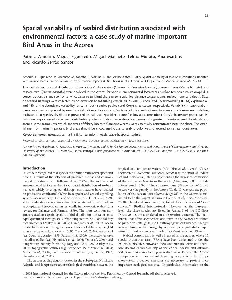
by narrow shelves. The Azorean exclusive economic zone (EEZ)crosses the Mid-Atlantic Ridge in the Northeast Atlantic Oceanand encloses an area of almost 1 million km2. This study wasconducted in a rectangular area of �226 000 km2 (368390 –398580N and 248260 –318260W), which includes most of thespatial data existing on seabirds (Figure 1).

Seabird dataData on seabirds were collected during the Azores FisheriesObservers Programme (POPA; www.popaobserver.org). The pro-gramme runs with trained observers on board fishing vessels,recording georeferenced data on fishing activities and otherrelevant information, such as sightings of associated species ofcetaceans, seabirds, and sea turtles (Feio et al., 2005; Macheteand Santos, 2007; Morato et al., 2008a). Data on seabird sightings

Figure 1. Location of the seabird snapshot counts conducted in the Azores, 2002–2006 (n ¼ 9183). The outline shape in the inset representsthe EEZ of the Azores.

. . . . . . . . . . . . . . . . . . . . . . . . . . . . . .. . . . . . . . . . . . . . . . . . . . . . . . . . . . . . . . . . . .. . . . . . . . . . . . . . . . . . . . . . . . . . .. . . . . . . . . . . . . . . . . . . . . . . . . . . . . . . . . . . . . . . . . . . . . . .. . . . . . . . . . . . . . . . . . . . . . . . . . . . . . . . . . . .. . . . . . . . . . . . . . . . . . . . . . . . . . . . . . . . . . . . . . . . . . . . . . . . . . . . . . . . . . . . . . . . . . . . . . . . . . . . . . . . . . . . .

. . . . . . . . . . . . . . . . . . . . . . . . . . . . . .. . . . . . . . . . . . . . . . . . . . . . . . . . . . . . . . . . . .. . . . . . . . . . . . . . . . . . . . . . . . . . .. . . . . . . . . . . . . . . . . . . . . . . . . . . . . . . . . . . . . . . . . . . . . . .. . . . . . . . . . . . . . . . . . . . . . . . . . . . . . . . . . . .. . . . . . . . . . . . . . . . . . . . . . . . . . . . . . . . . . . . . . . . . . . . . . . . . . . . . . . . . . . . . . . . . . . . . . . . . . . . . . . . . . . . .

Table 1. Cory’s shearwater and tern breeding and feeding characteristics in the Azores (adapted from Monteiro et al., 1996a, b; Neves,2007).

Species Breeding sites Breedingpairs

Period in Azores Nesting Main prey

Cory’sshearwater

All islands 160 000 Late February until lateOctober

Late May untilearly June

Small pelagic fish, small squids, crustaceans, andzooplankton (occasionally)

Common tern All islands 2 805 March–April until lateSeptember

Early May untilmid-July

Small and juvenile fish

Roseate tern All islands exceptCorvo

1 100 March–April until lateSeptember

Early May untilmid-July

Small and juvenile fish

30 P. Amorim et al.

were collected using a snapshot type of methodology, i.e. countingseabirds sighted around the boat (up to 300 m) during six dailyfixed periods, separated by 2-h intervals (09:00, 11:00, 13:00,15:00, 17:00, and 19:00). If no seabirds were observed, a zerocount was recorded. Otherwise, seabird sightings were recordedin quantity ranges (shearwaters: 1–10, 11–25, 26–50, 51–100,101–250, 251–500, 501–1000, and .1000; terns: 1–3, 4–10,11–25, 26–50, 51–75, 76–100, and .100). These categoricaldata were converted into continuous variables by assigning themean value of each class of abundance. We used data collectedduring 9183 snapshot counts performed from May to October,2002–2006. During this period, the most frequently observed sea-birds were Cory’s shearwater, common and roseate terns (pooled),and the yellow-legged gull (Larus michahellis atlantis). However, inthis study, we will focus on the first three species because of theirconservation-concern status.

Environmental dataSST in the Azores was obtained by satellite imagery at the “HAZO”HRPT station (http://oceano.horta.uac.pt/detra/), using theadvanced, very high-resolution radiometer (AVHRR) sensor. Chla was obtained using the MODIS sensor of the Aqua satellite(http://oceancolor.gsfc.nasa.gov/). Images were processed atIMAR-DOP/UAc (Figueiredo et al., 2004). Monthly medianvalues of SST and Chl a were obtained with a resolution of�1.2 � 1.2 km, 2002–2006.

Distances to productivity fronts are defined as discontinuityareas that presented simultaneously values of SST lower andvalues of Chl a higher than their adjacent areas. These distanceswere estimated using the methodology developed by Valavaniset al. (2005) and produced monthly mean grids of productivityfronts with a resolution of 1.852 � 1.852 km.

Information on wind was obtained with a resolution of �55 �55 km from QuikSCAT satellite imagery (http://www.ifremer.fr/cersat/en/general/general.htm), processed and distributed bythe Centre ERS d’Archivage et de Traitement at IFREMER,Plouzane, France. Wind components (speed, divergence, zonal,and meridional) were subsampled using the inverse distanceweighting to produce monthly mean grids of 1.852 � 1.852 km.

Additionally, depth, seabed slope, minimum distance to shore(islands), minimum distance to tern colonies, and minimum dis-tance to large and shallow seamounts were calculated for each cell.Depth was estimated using a bathymetry grid 1.85 � 1.85 km(Lourenco et al., 1998), and the slope angle (in degrees) was calcu-lated with the slope algorithm (in the ArcGIS software, ESRIArcMap 9.1). The location of large seamounts (.1000 mheight) and shallow seamounts (summit up to 300-m depth)was obtained from Morato et al. (2008b).

Statistical analysisMean monthly values of seabird counts and environmental vari-ables were estimated for each sampled cell of 1.852 � 1.852 kmfor the period 2002–2006. Pearson correlation coefficients werecalculated between all the environmental parameters to test forpossible covariation. The same coefficients were also calculatedbetween the mean numbers of seabirds sighted (log transformed)and the mean value of each environmental variable, by cell, todetermine potential linear relationships (Dalgaard, 2002).

Generalized linear models (GLM) were used to determine ifvariability in seabird sightings was significantly explained byenvironmental parameters. Monthly mean values of seabird sight-ings and environmental data (SST, Chl a, distance to fronts,and wind components) by cell were pooled, and “month” wasintegrated in the GLM as a categorical temporal variable.A quasi-Poisson family of probability distributions was usedwith the log-link function because of the large number of zerocounts (i.e. overdispersion). Seabed slope and distance to shore/

. . . . . . . . . . . . . . . . . . . . . . . .. . . . . . . . . . . . . . . . . . . . . . . .. . . . . . . . . . . . . . . . . . . . . . . . . . . . . .. . . . . . . . . . . . . . . . . . . . . . . . . . .. . . . . . . . . . . . . . . . . . . . . . .

. . . . . . . . . . . . . . . . . . . . . . . .. . . . . . . . . . . . . . . . . . . . . . . .. . . . . . . . . . . . . . . . . . . . . . . . . . . . . .. . . . . . . . . . . . . . . . . . . . . . . . . . .. . . . . . . . . . . . . . . . . . . . . . .

. . . . . . . . . . . . . . . . . . . . . . . .. . . . . . . . . . . . . . . . . . . . . . . .. . . . . . . . . . . . . . . . . . . . . . . . . . . . . .. . . . . . . . . . . . . . . . . . . . . . . . . . .. . . . . . . . . . . . . . . . . . . . . . .

. . . . . . . . . . . . . . . . . . . . . . . .. . . . . . . . . . . . . . . . . . . . . . . .. . . . . . . . . . . . . . . . . . . . . . . . . . . . . .. . . . . . . . . . . . . . . . . . . . . . . . . . .. . . . . . . . . . . . . . . . . . . . . . .

. . . . . . . . . . . . . . . . . . . . . . . .. . . . . . . . . . . . . . . . . . . . . . . .. . . . . . . . . . . . . . . . . . . . . . . . . . . . . .. . . . . . . . . . . . . . . . . . . . . . . . . . .. . . . . . . . . . . . . . . . . . . . . . .

Table 2. Monthly survey effort and seabird observations using thesnapshot method.

Month Snapshots Counts withbirds (%)

Mean (+++++s.d.; individualsper sighting)

Shearwaters Terns

May 1 164 84.0 22.7 (+80.4) 0.4 (+9.7)

June 2 132 76.6 23.4 (+61.4) 0.8 (+5.2)

July 2 271 74.5 37.2 (+87.7) 2.9 (+13.1)

August 2 309 87.3 53.8 (+100.9) 13.9 (+15.4)

September 1 088 88.3 17.6 (+67.6) 5.1 (+14.9)

October 219 88.6 2.0 (+25.4) 0.2 (+7.7)

The standard deviation is represented by s.d.

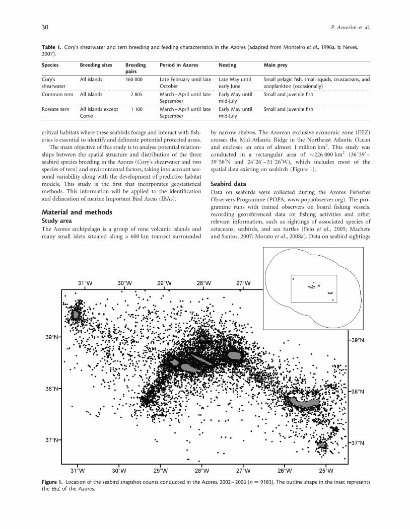
Figure 2. Monthly mean values of the median SST and the median chlorophyll-a (Chl a) concentration in the sampled area, 2002–2006.Vertical bars indicate standard deviation values. SST missing data: November and December 2004; Chl a missing data: January–May 2002.

Marine Important Bird Areas in the Azores 31

. . . . . . . . . . . . . . . . . . . . . . . . . . . . . . . . . . . . . . . . . . . . . . . . .. . . . . . . . . . . . . . . . .. . . . . . . . . . . . . . . . . . . . . . . . . .. . . . . . . . . . . . . . . . . . . . . . . . . . .. . . . . . . . . . . . . . . . . . . . . . . . . . . . . . . . . . . .. . . . . . . . . . . . . . . . .. . . . . . . . . . . . . . . . .. . . . . . . . . . . . .. . . . . . . . . . . . . . . . . . . . . . . . . .. . . . . . . . . . . . . . . . . . . . . . . . . . . . .. . . . . . . . . . . . . . . . . . . . . . . . . . . . .. . . . . . . . . . . . . . . . . . . . . . . . .. . . . . . . . . . . . . . . . . . . .. . . . . . . . . . . . . . . . . . . . . . . . . .

. . . . . . . . . . . . . . . . . . . . . . . . . . . . . . . . . . . . . . . . . . . . . . . . .. . . . . . . . . . . . . . . . .. . . . . . . . . . . . . . . . . . . . . . . . . .. . . . . . . . . . . . . . . . . . . . . . . . . . .. . . . . . . . . . . . . . . . . . . . . . . . . . . . . . . . . . . .. . . . . . . . . . . . . . . . .. . . . . . . . . . . . . . . . .. . . . . . . . . . . . .. . . . . . . . . . . . . . . . . . . . . . . . . .. . . . . . . . . . . . . . . . . . . . . . . . . . . . .. . . . . . . . . . . . . . . . . . . . . . . . . . . . .. . . . . . . . . . . . . . . . . . . . . . . . .. . . . . . . . . . . . . . . . . . . .. . . . . . . . . . . . . . . . . . . . . . . . . .

. . . . . . . . . . . . . . . . . . . . . . . . . . . . . . . . . . . . . . . . . . . . . . . . .. . . . . . . . . . . . . . . . .. . . . . . . . . . . . . . . . . . . . . . . . . .. . . . . . . . . . . . . . . . . . . . . . . . . . .. . . . . . . . . . . . . . . . . . . . . . . . . . . . . . . . . . . .. . . . . . . . . . . . . . . . .. . . . . . . . . . . . . . . . .. . . . . . . . . . . . .. . . . . . . . . . . . . . . . . . . . . . . . . .. . . . . . . . . . . . . . . . . . . . . . . . . . . . .. . . . . . . . . . . . . . . . . . . . . . . . . . . . .. . . . . . . . . . . . . . . . . . . . . . . . .. . . . . . . . . . . . . . . . . . . .. . . . . . . . . . . . . . . . . . . . . . . . . .

. . . . . . . . . . . . . . . . . . . . . . . . . . . . . . . . . . . . . . . . . . . . . . . . .. . . . . . . . . . . . . . . . .. . . . . . . . . . . . . . . . . . . . . . . . . .. . . . . . . . . . . . . . . . . . . . . . . . . . .. . . . . . . . . . . . . . . . . . . . . . . . . . . . . . . . . . . .. . . . . . . . . . . . . . . . .. . . . . . . . . . . . . . . . .. . . . . . . . . . . . .. . . . . . . . . . . . . . . . . . . . . . . . . .. . . . . . . . . . . . . . . . . . . . . . . . . . . . .. . . . . . . . . . . . . . . . . . . . . . . . . . . . .. . . . . . . . . . . . . . . . . . . . . . . . .. . . . . . . . . . . . . . . . . . . .. . . . . . . . . . . . . . . . . . . . . . . . . .

. . . . . . . . . . . . . . . . . . . . . . . . . . . . . . . . . . . . . . . . . . . . . . . . .. . . . . . . . . . . . . . . . .. . . . . . . . . . . . . . . . . . . . . . . . . .. . . . . . . . . . . . . . . . . . . . . . . . . . .. . . . . . . . . . . . . . . . . . . . . . . . . . . . . . . . . . . .. . . . . . . . . . . . . . . . .. . . . . . . . . . . . . . . . .. . . . . . . . . . . . .. . . . . . . . . . . . . . . . . . . . . . . . . .. . . . . . . . . . . . . . . . . . . . . . . . . . . . .. . . . . . . . . . . . . . . . . . . . . . . . . . . . .. . . . . . . . . . . . . . . . . . . . . . . . .. . . . . . . . . . . . . . . . . . . .. . . . . . . . . . . . . . . . . . . . . . . . . .

. . . . . . . . . . . . . . . . . . . . . . . . . . . . . . . . . . . . . . . . . . . . . . . . .. . . . . . . . . . . . . . . . .. . . . . . . . . . . . . . . . . . . . . . . . . .. . . . . . . . . . . . . . . . . . . . . . . . . . .. . . . . . . . . . . . . . . . . . . . . . . . . . . . . . . . . . . .. . . . . . . . . . . . . . . . .. . . . . . . . . . . . . . . . .. . . . . . . . . . . . .. . . . . . . . . . . . . . . . . . . . . . . . . .. . . . . . . . . . . . . . . . . . . . . . . . . . . . .. . . . . . . . . . . . . . . . . . . . . . . . . . . . .. . . . . . . . . . . . . . . . . . . . . . . . .. . . . . . . . . . . . . . . . . . . .. . . . . . . . . . . . . . . . . . . . . . . . . .

. . . . . . . . . . . . . . . . . . . . . . . . . . . . . . . . . . . . . . . . . . . . . . . . .. . . . . . . . . . . . . . . . .. . . . . . . . . . . . . . . . . . . . . . . . . .. . . . . . . . . . . . . . . . . . . . . . . . . . .. . . . . . . . . . . . . . . . . . . . . . . . . . . . . . . . . . . .. . . . . . . . . . . . . . . . .. . . . . . . . . . . . . . . . .. . . . . . . . . . . . .. . . . . . . . . . . . . . . . . . . . . . . . . .. . . . . . . . . . . . . . . . . . . . . . . . . . . . .. . . . . . . . . . . . . . . . . . . . . . . . . . . . .. . . . . . . . . . . . . . . . . . . . . . . . .. . . . . . . . . . . . . . . . . . . .. . . . . . . . . . . . . . . . . . . . . . . . . .

. . . . . . . . . . . . . . . . . . . . . . . . . . . . . . . . . . . . . . . . . . . . . . . . .. . . . . . . . . . . . . . . . .. . . . . . . . . . . . . . . . . . . . . . . . . .. . . . . . . . . . . . . . . . . . . . . . . . . . .. . . . . . . . . . . . . . . . . . . . . . . . . . . . . . . . . . . .. . . . . . . . . . . . . . . . .. . . . . . . . . . . . . . . . .. . . . . . . . . . . . .. . . . . . . . . . . . . . . . . . . . . . . . . .. . . . . . . . . . . . . . . . . . . . . . . . . . . . .. . . . . . . . . . . . . . . . . . . . . . . . . . . . .. . . . . . . . . . . . . . . . . . . . . . . . .. . . . . . . . . . . . . . . . . . . .. . . . . . . . . . . . . . . . . . . . . . . . . .

. . . . . . . . . . . . . . . . . . . . . . . . . . . . . . . . . . . . . . . . . . . . . . . . .. . . . . . . . . . . . . . . . .. . . . . . . . . . . . . . . . . . . . . . . . . .. . . . . . . . . . . . . . . . . . . . . . . . . . .. . . . . . . . . . . . . . . . . . . . . . . . . . . . . . . . . . . .. . . . . . . . . . . . . . . . .. . . . . . . . . . . . . . . . .. . . . . . . . . . . . .. . . . . . . . . . . . . . . . . . . . . . . . . .. . . . . . . . . . . . . . . . . . . . . . . . . . . . .. . . . . . . . . . . . . . . . . . . . . . . . . . . . .. . . . . . . . . . . . . . . . . . . . . . . . .. . . . . . . . . . . . . . . . . . . .. . . . . . . . . . . . . . . . . . . . . . . . . .

. . . . . . . . . . . . . . . . . . . . . . . . . . . . . . . . . . . . . . . . . . . . . . . . .. . . . . . . . . . . . . . . . .. . . . . . . . . . . . . . . . . . . . . . . . . .. . . . . . . . . . . . . . . . . . . . . . . . . . .. . . . . . . . . . . . . . . . . . . . . . . . . . . . . . . . . . . .. . . . . . . . . . . . . . . . .. . . . . . . . . . . . . . . . .. . . . . . . . . . . . .. . . . . . . . . . . . . . . . . . . . . . . . . .. . . . . . . . . . . . . . . . . . . . . . . . . . . . .. . . . . . . . . . . . . . . . . . . . . . . . . . . . .. . . . . . . . . . . . . . . . . . . . . . . . .. . . . . . . . . . . . . . . . . . . .. . . . . . . . . . . . . . . . . . . . . . . . . .

. . . . . . . . . . . . . . . . . . . . . . . . . . . . . . . . . . . . . . . . . . . . . . . . .. . . . . . . . . . . . . . . . .. . . . . . . . . . . . . . . . . . . . . . . . . .. . . . . . . . . . . . . . . . . . . . . . . . . . .. . . . . . . . . . . . . . . . . . . . . . . . . . . . . . . . . . . .. . . . . . . . . . . . . . . . .. . . . . . . . . . . . . . . . .. . . . . . . . . . . . .. . . . . . . . . . . . . . . . . . . . . . . . . .. . . . . . . . . . . . . . . . . . . . . . . . . . . . .. . . . . . . . . . . . . . . . . . . . . . . . . . . . .. . . . . . . . . . . . . . . . . . . . . . . . .. . . . . . . . . . . . . . . . . . . .. . . . . . . . . . . . . . . . . . . . . . . . . .

. . . . . . . . . . . . . . . . . . . . . . . . . . . . . . . . . . . . . . . . . . . . . . . . .. . . . . . . . . . . . . . . . .. . . . . . . . . . . . . . . . . . . . . . . . . .. . . . . . . . . . . . . . . . . . . . . . . . . . .. . . . . . . . . . . . . . . . . . . . . . . . . . . . . . . . . . . .. . . . . . . . . . . . . . . . .. . . . . . . . . . . . . . . . .. . . . . . . . . . . . .. . . . . . . . . . . . . . . . . . . . . . . . . .. . . . . . . . . . . . . . . . . . . . . . . . . . . . .. . . . . . . . . . . . . . . . . . . . . . . . . . . . .. . . . . . . . . . . . . . . . . . . . . . . . .. . . . . . . . . . . . . . . . . . . .. . . . . . . . . . . . . . . . . . . . . . . . . .

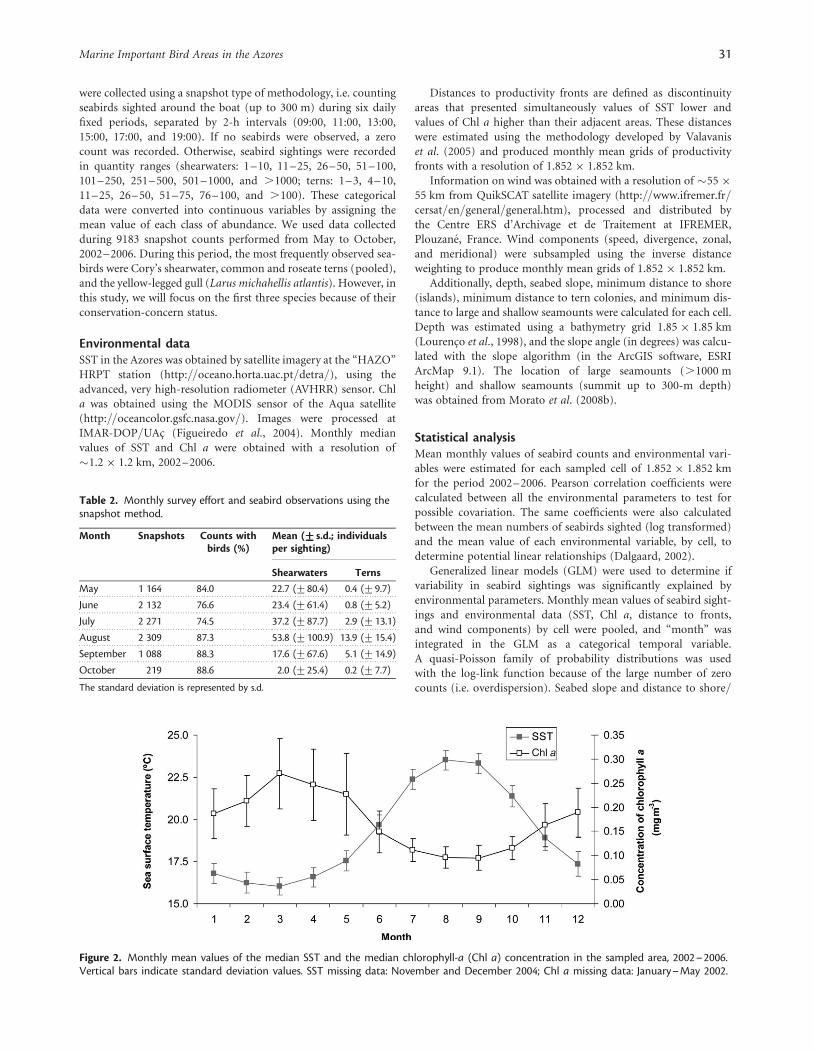
Table 3. Pearson correlation coefficients calculated between all environmental variables.

Parameter Depth Distanceshore

Distanceseamounts

Distance shallowseamounts

Slope SST Chla

Distancefronts

Winddivergence

Windmeridional

Windspeed Windzonal

Distance terncolonies

Depth 1

Distance shore 0.37 1

Distance seamounts 0.08 20.34 1

Distance shallowseamounts

0.06 20.11 0.60 1

Slope 20.24 20.28 20.01 20.04 1

SST 20.10 20.09 0.14 0.26 0.10 1

Chl a 20.09 0.05 20.09 20.14 20.07 20.52 1

Distance fronts 0.09 20.14 0.13 0.03 0.03 20.15 0.01 1

Wind divergence 20.07 20.08 20.11 20.06 0.02 20.01 0.22 20.02 1

Wind meridional 20.02 20.01 0.08 20.02 20.03 20.21 0.24 0.18 20.12 1

Windspeed 20.11 20.05 20.06 20.11 0.01 20.39 0.09 0.02 20.28 0.07 1

Wind zonal 0.01 0.14 0.03 0.03 20.07 20.28 0.26 0.02 0.05 0.12 0.39 1

Distance tern colonies 0.38 1.00 20.34 20.11 20.28 20.10 0.05 20.12 20.09 20.01 20.04 0.14 1

SST, sea surface temperature; chl a, chlorophyll a.Emboldened values indicate significant correlations (p-value , 0.01).

32P.

Am

orimet

al.

colonies were log10-transformed to achieve normality. Linear andquadratic relationships between seabird abundance and environ-mental variables were fitted. All models were built by a forwardstepwise selection of variables, adding the significant terms (a �0.05) sequentially. Thereafter, non-significant variables weredeleted from the final model (Bio, 2000). The final adjustmentof the model was made by the analysis of the pseudo-determination coefficient (pseudo-R2), i.e. the fraction of thetotal variability explained by the model.

Additionally, to investigate whether or not different parametersmight be affecting shearwater abundance close to colonies and off-shore feeding areas, the shearwater sightings data were divided intotwo datasets: (i) onshore (based on sightings undertaken up to30 km from shore; n ¼ 4419) and offshore (distance to shore�30 km; n ¼ 2532). This break was selected based on the resultsof the general model that indicated an accentuated decrease inthe number of shearwaters �30 km from shore.

Because the variance caused by autocorrelation cannot be prop-erly quantified by the GLMs, the seabird spatial structure wasanalysed using geostatistical methods by (i) modelling the spatialstructure of the seabirds through the variogram fit and (ii) estimat-ing the seabird distribution through kriging techniques. Theresiduals were transformed to achieve a constant variance.Standardized Pearson residuals were analysed through the vario-gram fit to assess spatial autocorrelation (Pebesma, 2004; Pebesmaet al., 2005), considering geometric anisotropy and based on thespherical model. The parameters of each model—nugget effect(the discontinuity at the origin), sill (variance of the randomfield), range (distance beyond which the observations are not corre-lated), and direction—were determined by an interactive process.

The spatial component was added to the GLM results to yield aprediction of the seabird distribution based on the predictorvariables (environmental parameters) and on the part of spatialstructure of the seabirds (autocorrelation) to improve the accuracyof seabird numbers estimates. Spatial prediction for the wholestudy area was performed through block kriging (Pebesma,2004). The mean error and the percentage of dispersion of theerror in relation to sample mean were calculated to compare theobserved and predicted values.

ResultsSeabird sightingsIn all, 9183 snapshot counts were performed during the studyperiod (May–October 2002–2006), with the highest effort June–August (Table 2). Seabirds occurred in more than 80% of all snap-shots, with Cory’s shearwaters observed in 64% of the snapshots andterns in only 25%. The mean number of seabirds sighted variedamong species, with a mean of �20 shearwaters and three ternsobserved per snapshot. There were monthly differences in meanseabird numbers, with a peak in August for both taxa (Table 2).

Environmental dataThe monthly mean values obtained from the median SST and Chla images, 2002–2006, varied seasonally (Figure 2). SST around theAzores ranged from 16.08C to 23.58C, and near-surface Chl aranged from 0.1 to 0.3 mg m23. Comparison of monthly SSTand Chl a values revealed an out-of-phase seasonal response,with periods of higher temperatures associated with lower Chl a(Figure 2) showing a significant negative correlation (r ¼2 0.52,p , 0.01, n ¼ 6950; Table 3).

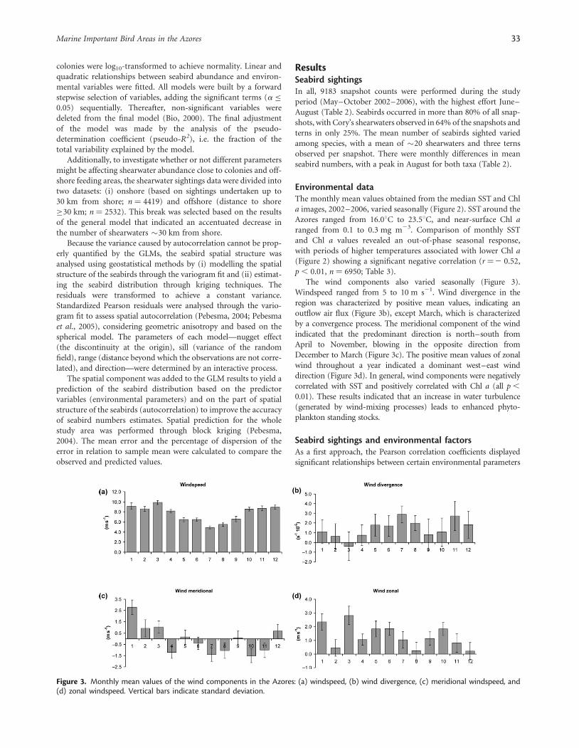
The wind components also varied seasonally (Figure 3).Windspeed ranged from 5 to 10 m s21. Wind divergence in theregion was characterized by positive mean values, indicating anoutflow air flux (Figure 3b), except March, which is characterizedby a convergence process. The meridional component of the windindicated that the predominant direction is north–south fromApril to November, blowing in the opposite direction fromDecember to March (Figure 3c). The positive mean values of zonalwind throughout a year indicated a dominant west–east winddirection (Figure 3d). In general, wind components were negativelycorrelated with SST and positively correlated with Chl a (all p ,

0.01). These results indicated that an increase in water turbulence(generated by wind-mixing processes) leads to enhanced phyto-plankton standing stocks.

Seabird sightings and environmental factorsAs a first approach, the Pearson correlation coefficients displayedsignificant relationships between certain environmental parameters

Figure 3. Monthly mean values of the wind components in the Azores: (a) windspeed, (b) wind divergence, (c) meridional windspeed, and(d) zonal windspeed. Vertical bars indicate standard deviation.

Marine Important Bird Areas in the Azores 33

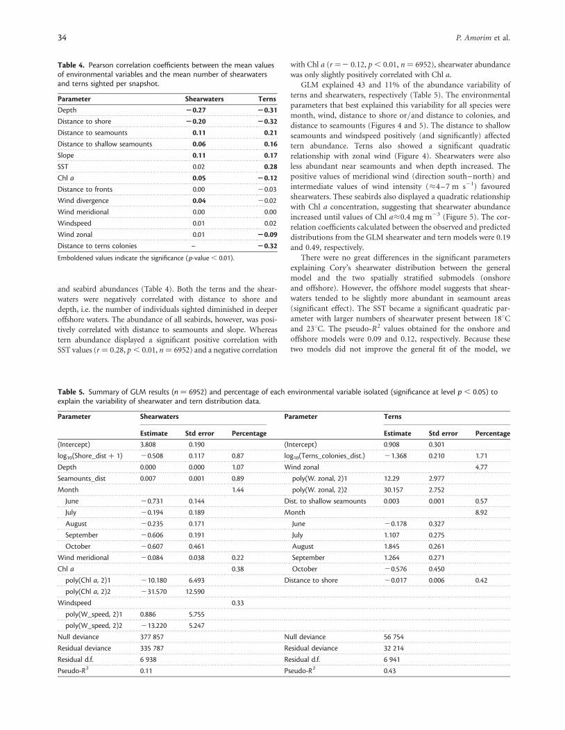
and seabird abundances (Table 4). Both the terns and the shear-waters were negatively correlated with distance to shore anddepth, i.e. the number of individuals sighted diminished in deeperoffshore waters. The abundance of all seabirds, however, was posi-tively correlated with distance to seamounts and slope. Whereastern abundance displayed a significant positive correlation withSST values (r ¼ 0.28, p , 0.01, n ¼ 6952) and a negative correlation

with Chl a (r ¼2 0.12, p , 0.01, n ¼ 6952), shearwater abundancewas only slightly positively correlated with Chl a.

GLM explained 43 and 11% of the abundance variability ofterns and shearwaters, respectively (Table 5). The environmentalparameters that best explained this variability for all species weremonth, wind, distance to shore or/and distance to colonies, anddistance to seamounts (Figures 4 and 5). The distance to shallowseamounts and windspeed positively (and significantly) affectedtern abundance. Terns also showed a significant quadraticrelationship with zonal wind (Figure 4). Shearwaters were alsoless abundant near seamounts and when depth increased. Thepositive values of meridional wind (direction south–north) andintermediate values of wind intensity (�4–7 m s21) favouredshearwaters. These seabirds also displayed a quadratic relationshipwith Chl a concentration, suggesting that shearwater abundanceincreased until values of Chl a�0.4 mg m23 (Figure 5). The cor-relation coefficients calculated between the observed and predicteddistributions from the GLM shearwater and tern models were 0.19and 0.49, respectively.

There were no great differences in the significant parametersexplaining Cory’s shearwater distribution between the generalmodel and the two spatially stratified submodels (onshoreand offshore). However, the offshore model suggests that shear-waters tended to be slightly more abundant in seamount areas(significant effect). The SST became a significant quadratic par-ameter with larger numbers of shearwater present between 188Cand 238C. The pseudo-R2 values obtained for the onshore andoffshore models were 0.09 and 0.12, respectively. Because thesetwo models did not improve the general fit of the model, we

. . . . . . . . . . . . . . . . . . . . . . . . . . . . . . . . . . . . . . . . . . . . . . . . . . . . . . . . . . . . . . . . . . . . . . . . . .. . . . . . . . . . . . . . . . . . . . . . . . . . . . . . . . . . . . . . . . .. . . . . . . . . . . .

. . . . . . . . . . . . . . . . . . . . . . . . . . . . . . . . . . . . . . . . . . . . . . . . . . . . . . . . . . . . . . . . . . . . . . . . . .. . . . . . . . . . . . . . . . . . . . . . . . . . . . . . . . . . . . . . . . .. . . . . . . . . . . .

. . . . . . . . . . . . . . . . . . . . . . . . . . . . . . . . . . . . . . . . . . . . . . . . . . . . . . . . . . . . . . . . . . . . . . . . . .. . . . . . . . . . . . . . . . . . . . . . . . . . . . . . . . . . . . . . . . .. . . . . . . . . . . .

. . . . . . . . . . . . . . . . . . . . . . . . . . . . . . . . . . . . . . . . . . . . . . . . . . . . . . . . . . . . . . . . . . . . . . . . . .. . . . . . . . . . . . . . . . . . . . . . . . . . . . . . . . . . . . . . . . .. . . . . . . . . . . .

. . . . . . . . . . . . . . . . . . . . . . . . . . . . . . . . . . . . . . . . . . . . . . . . . . . . . . . . . . . . . . . . . . . . . . . . . .. . . . . . . . . . . . . . . . . . . . . . . . . . . . . . . . . . . . . . . . .. . . . . . . . . . . .

. . . . . . . . . . . . . . . . . . . . . . . . . . . . . . . . . . . . . . . . . . . . . . . . . . . . . . . . . . . . . . . . . . . . . . . . . .. . . . . . . . . . . . . . . . . . . . . . . . . . . . . . . . . . . . . . . . .. . . . . . . . . . . .

. . . . . . . . . . . . . . . . . . . . . . . . . . . . . . . . . . . . . . . . . . . . . . . . . . . . . . . . . . . . . . . . . . . . . . . . . .. . . . . . . . . . . . . . . . . . . . . . . . . . . . . . . . . . . . . . . . .. . . . . . . . . . . .

. . . . . . . . . . . . . . . . . . . . . . . . . . . . . . . . . . . . . . . . . . . . . . . . . . . . . . . . . . . . . . . . . . . . . . . . . .. . . . . . . . . . . . . . . . . . . . . . . . . . . . . . . . . . . . . . . . .. . . . . . . . . . . .

. . . . . . . . . . . . . . . . . . . . . . . . . . . . . . . . . . . . . . . . . . . . . . . . . . . . . . . . . . . . . . . . . . . . . . . . . .. . . . . . . . . . . . . . . . . . . . . . . . . . . . . . . . . . . . . . . . .. . . . . . . . . . . .

. . . . . . . . . . . . . . . . . . . . . . . . . . . . . . . . . . . . . . . . . . . . . . . . . . . . . . . . . . . . . . . . . . . . . . . . . .. . . . . . . . . . . . . . . . . . . . . . . . . . . . . . . . . . . . . . . . .. . . . . . . . . . . .

. . . . . . . . . . . . . . . . . . . . . . . . . . . . . . . . . . . . . . . . . . . . . . . . . . . . . . . . . . . . . . . . . . . . . . . . . .. . . . . . . . . . . . . . . . . . . . . . . . . . . . . . . . . . . . . . . . .. . . . . . . . . . . .

. . . . . . . . . . . . . . . . . . . . . . . . . . . . . . . . . . . . . . . . . . . . . . . . . . . . . . . . . . . . . . . . . . . . . . . . . .. . . . . . . . . . . . . . . . . . . . . . . . . . . . . . . . . . . . . . . . .. . . . . . . . . . . .

Table 4. Pearson correlation coefficients between the mean valuesof environmental variables and the mean number of shearwatersand terns sighted per snapshot.

Parameter Shearwaters Terns

Depth 20.27 20.31

Distance to shore 20.20 20.32

Distance to seamounts 0.11 0.21

Distance to shallow seamounts 0.06 0.16

Slope 0.11 0.17

SST 0.02 0.28

Chl a 0.05 20.12

Distance to fronts 0.00 20.03

Wind divergence 0.04 20.02

Wind meridional 0.00 0.00

Windspeed 0.01 0.02

Wind zonal 0.01 20.09

Distance to terns colonies – 20.32

Emboldened values indicate the significance (p-value , 0.01).

. . . . . . . . . . . . . . . . . . . . . . . . . . . . . . . . . . . . . . . . . . . . . . . .. . . . . . . . . . . . . . . . . . . . . . . . . .. . . . . . . . . . . . . . . . . . . . . . . . . . .. . . . . . . . . . . . . . . . . . . . . . . . . . . . . .. . . . . . . . . . . . . . . . . . . . . . . . . . . . . . . . . . . . . . . . . . . . . . . . . . . . . . . . . .. . . . . . . . . . . . . . . . . . . . . . . . . .. . . . . . . . . . . . . . . . . . . . . . . . . . .. . . . . . . . . . . . . . . . . . . .

. . . . . . . . . . . . . . . . . . . . . . . . . . . . . . . . . . . . . . . . . . . . . . . .. . . . . . . . . . . . . . . . . . . . . . . . . .. . . . . . . . . . . . . . . . . . . . . . . . . . .. . . . . . . . . . . . . . . . . . . . . . . . . . . . . .. . . . . . . . . . . . . . . . . . . . . . . . . . . . . . . . . . . . . . . . . . . . . . . . . . . . . . . . . .. . . . . . . . . . . . . . . . . . . . . . . . . .. . . . . . . . . . . . . . . . . . . . . . . . . . .. . . . . . . . . . . . . . . . . . . .

. . . . . . . . . . . . . . . . . . . . . . . . . . . . . . . . . . . . . . . . . . . . . . . .. . . . . . . . . . . . . . . . . . . . . . . . . .. . . . . . . . . . . . . . . . . . . . . . . . . . .. . . . . . . . . . . . . . . . . . . . . . . . . . . . . .. . . . . . . . . . . . . . . . . . . . . . . . . . . . . . . . . . . . . . . . . . . . . . . . . . . . . . . . . .. . . . . . . . . . . . . . . . . . . . . . . . . .. . . . . . . . . . . . . . . . . . . . . . . . . . .. . . . . . . . . . . . . . . . . . . .

. . . . . . . . . . . . . . . . . . . . . . . . . . . . . . . . . . . . . . . . . . . . . . . .. . . . . . . . . . . . . . . . . . . . . . . . . .. . . . . . . . . . . . . . . . . . . . . . . . . . .. . . . . . . . . . . . . . . . . . . . . . . . . . . . . .. . . . . . . . . . . . . . . . . . . . . . . . . . . . . . . . . . . . . . . . . . . . . . . . . . . . . . . . . .. . . . . . . . . . . . . . . . . . . . . . . . . .. . . . . . . . . . . . . . . . . . . . . . . . . . .. . . . . . . . . . . . . . . . . . . .

. . . . . . . . . . . . . . . . . . . . . . . . . . . . . . . . . . . . . . . . . . . . . . . .. . . . . . . . . . . . . . . . . . . . . . . . . .. . . . . . . . . . . . . . . . . . . . . . . . . . .. . . . . . . . . . . . . . . . . . . . . . . . . . . . . .. . . . . . . . . . . . . . . . . . . . . . . . . . . . . . . . . . . . . . . . . . . . . . . . . . . . . . . . . .. . . . . . . . . . . . . . . . . . . . . . . . . .. . . . . . . . . . . . . . . . . . . . . . . . . . .. . . . . . . . . . . . . . . . . . . .

. . . . . . . . . . . . . . . . . . . . . . . . . . . . . . . . . . . . . . . . . . . . . . . .. . . . . . . . . . . . . . . . . . . . . . . . . .. . . . . . . . . . . . . . . . . . . . . . . . . . .. . . . . . . . . . . . . . . . . . . . . . . . . . . . . .. . . . . . . . . . . . . . . . . . . . . . . . . . . . . . . . . . . . . . . . . . . . . . . . . . . . . . . . . .. . . . . . . . . . . . . . . . . . . . . . . . . .. . . . . . . . . . . . . . . . . . . . . . . . . . .. . . . . . . . . . . . . . . . . . . .

. . . . . . . . . . . . . . . . . . . . . . . . . . . . . . . . . . . . . . . . . . . . . . . .. . . . . . . . . . . . . . . . . . . . . . . . . .. . . . . . . . . . . . . . . . . . . . . . . . . . .. . . . . . . . . . . . . . . . . . . . . . . . . . . . . .. . . . . . . . . . . . . . . . . . . . . . . . . . . . . . . . . . . . . . . . . . . . . . . . . . . . . . . . . .. . . . . . . . . . . . . . . . . . . . . . . . . .. . . . . . . . . . . . . . . . . . . . . . . . . . .. . . . . . . . . . . . . . . . . . . .

. . . . . . . . . . . . . . . . . . . . . . . . . . . . . . . . . . . . . . . . . . . . . . . .. . . . . . . . . . . . . . . . . . . . . . . . . .. . . . . . . . . . . . . . . . . . . . . . . . . . .. . . . . . . . . . . . . . . . . . . . . . . . . . . . . .. . . . . . . . . . . . . . . . . . . . . . . . . . . . . . . . . . . . . . . . . . . . . . . . . . . . . . . . . .. . . . . . . . . . . . . . . . . . . . . . . . . .. . . . . . . . . . . . . . . . . . . . . . . . . . .. . . . . . . . . . . . . . . . . . . .

. . . . . . . . . . . . . . . . . . . . . . . . . . . . . . . . . . . . . . . . . . . . . . . .. . . . . . . . . . . . . . . . . . . . . . . . . .. . . . . . . . . . . . . . . . . . . . . . . . . . .. . . . . . . . . . . . . . . . . . . . . . . . . . . . . .. . . . . . . . . . . . . . . . . . . . . . . . . . . . . . . . . . . . . . . . . . . . . . . . . . . . . . . . . .. . . . . . . . . . . . . . . . . . . . . . . . . .. . . . . . . . . . . . . . . . . . . . . . . . . . .. . . . . . . . . . . . . . . . . . . .

. . . . . . . . . . . . . . . . . . . . . . . . . . . . . . . . . . . . . . . . . . . . . . . .. . . . . . . . . . . . . . . . . . . . . . . . . .. . . . . . . . . . . . . . . . . . . . . . . . . . .. . . . . . . . . . . . . . . . . . . . . . . . . . . . . .. . . . . . . . . . . . . . . . . . . . . . . . . . . . . . . . . . . . . . . . . . . . . . . . . . . . . . . . . .. . . . . . . . . . . . . . . . . . . . . . . . . .. . . . . . . . . . . . . . . . . . . . . . . . . . .. . . . . . . . . . . . . . . . . . . .

. . . . . . . . . . . . . . . . . . . . . . . . . . . . . . . . . . . . . . . . . . . . . . . .. . . . . . . . . . . . . . . . . . . . . . . . . .. . . . . . . . . . . . . . . . . . . . . . . . . . .. . . . . . . . . . . . . . . . . . . . . . . . . . . . . .. . . . . . . . . . . . . . . . . . . . . . . . . . . . . . . . . . . . . . . . . . . . . . . . . . . . . . . . . .. . . . . . . . . . . . . . . . . . . . . . . . . .. . . . . . . . . . . . . . . . . . . . . . . . . . .. . . . . . . . . . . . . . . . . . . .

. . . . . . . . . . . . . . . . . . . . . . . . . . . . . . . . . . . . . . . . . . . . . . . .. . . . . . . . . . . . . . . . . . . . . . . . . .. . . . . . . . . . . . . . . . . . . . . . . . . . .. . . . . . . . . . . . . . . . . . . . . . . . . . . . . .. . . . . . . . . . . . . . . . . . . . . . . . . . . . . . . . . . . . . . . . . . . . . . . . . . . . . . . . . .. . . . . . . . . . . . . . . . . . . . . . . . . .. . . . . . . . . . . . . . . . . . . . . . . . . . .. . . . . . . . . . . . . . . . . . . .

. . . . . . . . . . . . . . . . . . . . . . . . . . . . . . . . . . . . . . . . . . . . . . . .. . . . . . . . . . . . . . . . . . . . . . . . . .. . . . . . . . . . . . . . . . . . . . . . . . . . .. . . . . . . . . . . . . . . . . . . . . . . . . . . . . .. . . . . . . . . . . . . . . . . . . . . . . . . . . . . . . . . . . . . . . . . . . . . . . . . . . . . . . . . .. . . . . . . . . . . . . . . . . . . . . . . . . .. . . . . . . . . . . . . . . . . . . . . . . . . . .. . . . . . . . . . . . . . . . . . . .

. . . . . . . . . . . . . . . . . . . . . . . . . . . . . . . . . . . . . . . . . . . . . . . .. . . . . . . . . . . . . . . . . . . . . . . . . .. . . . . . . . . . . . . . . . . . . . . . . . . . .. . . . . . . . . . . . . . . . . . . . . . . . . . . . . .. . . . . . . . . . . . . . . . . . . . . . . . . . . . . . . . . . . . . . . . . . . . . . . . . . . . . . . . . .. . . . . . . . . . . . . . . . . . . . . . . . . .. . . . . . . . . . . . . . . . . . . . . . . . . . .. . . . . . . . . . . . . . . . . . . .

. . . . . . . . . . . . . . . . . . . . . . . . . . . . . . . . . . . . . . . . . . . . . . . .. . . . . . . . . . . . . . . . . . . . . . . . . .. . . . . . . . . . . . . . . . . . . . . . . . . . .. . . . . . . . . . . . . . . . . . . . . . . . . . . . . .. . . . . . . . . . . . . . . . . . . . . . . . . . . . . . . . . . . . . . . . . . . . . . . . . . . . . . . . . .. . . . . . . . . . . . . . . . . . . . . . . . . .. . . . . . . . . . . . . . . . . . . . . . . . . . .. . . . . . . . . . . . . . . . . . . .

. . . . . . . . . . . . . . . . . . . . . . . . . . . . . . . . . . . . . . . . . . . . . . . .. . . . . . . . . . . . . . . . . . . . . . . . . .. . . . . . . . . . . . . . . . . . . . . . . . . . .. . . . . . . . . . . . . . . . . . . . . . . . . . . . . .. . . . . . . . . . . . . . . . . . . . . . . . . . . . . . . . . . . . . . . . . . . . . . . . . . . . . . . . . .. . . . . . . . . . . . . . . . . . . . . . . . . .. . . . . . . . . . . . . . . . . . . . . . . . . . .. . . . . . . . . . . . . . . . . . . .

. . . . . . . . . . . . . . . . . . . . . . . . . . . . . . . . . . . . . . . . . . . . . . . .. . . . . . . . . . . . . . . . . . . . . . . . . .. . . . . . . . . . . . . . . . . . . . . . . . . . .. . . . . . . . . . . . . . . . . . . . . . . . . . . . . .. . . . . . . . . . . . . . . . . . . . . . . . . . . . . . . . . . . . . . . . . . . . . . . . . . . . . . . . . .. . . . . . . . . . . . . . . . . . . . . . . . . .. . . . . . . . . . . . . . . . . . . . . . . . . . .. . . . . . . . . . . . . . . . . . . .

. . . . . . . . . . . . . . . . . . . . . . . . . . . . . . . . . . . . . . . . . . . . . . . .. . . . . . . . . . . . . . . . . . . . . . . . . .. . . . . . . . . . . . . . . . . . . . . . . . . . .. . . . . . . . . . . . . . . . . . . . . . . . . . . . . .. . . . . . . . . . . . . . . . . . . . . . . . . . . . . . . . . . . . . . . . . . . . . . . . . . . . . . . . . .. . . . . . . . . . . . . . . . . . . . . . . . . .. . . . . . . . . . . . . . . . . . . . . . . . . . .. . . . . . . . . . . . . . . . . . . .

. . . . . . . . . . . . . . . . . . . . . . . . . . . . . . . . . . . . . . . . . . . . . . . .. . . . . . . . . . . . . . . . . . . . . . . . . .. . . . . . . . . . . . . . . . . . . . . . . . . . .. . . . . . . . . . . . . . . . . . . . . . . . . . . . . .. . . . . . . . . . . . . . . . . . . . . . . . . . . . . . . . . . . . . . . . . . . . . . . . . . . . . . . . . .. . . . . . . . . . . . . . . . . . . . . . . . . .. . . . . . . . . . . . . . . . . . . . . . . . . . .. . . . . . . . . . . . . . . . . . . .

. . . . . . . . . . . . . . . . . . . . . . . . . . . . . . . . . . . . . . . . . . . . . . . .. . . . . . . . . . . . . . . . . . . . . . . . . .. . . . . . . . . . . . . . . . . . . . . . . . . . .. . . . . . . . . . . . . . . . . . . . . . . . . . . . . .. . . . . . . . . . . . . . . . . . . . . . . . . . . . . . . . . . . . . . . . . . . . . . . . . . . . . . . . . .. . . . . . . . . . . . . . . . . . . . . . . . . .. . . . . . . . . . . . . . . . . . . . . . . . . . .. . . . . . . . . . . . . . . . . . . .

Table 5. Summary of GLM results (n ¼ 6952) and percentage of each environmental variable isolated (significance at level p , 0.05) toexplain the variability of shearwater and tern distribution data.

Parameter Shearwaters Parameter Terns

Estimate Std error Percentage Estimate Std error Percentage

(Intercept) 3.808 0.190 (Intercept) 0.908 0.301

log10(Shore_dist þ 1) 20.508 0.117 0.87 log10(Terns_colonies_dist.) 21.368 0.210 1.71

Depth 0.000 0.000 1.07 Wind zonal 4.77

Seamounts_dist 0.007 0.001 0.89 poly(W. zonal, 2)1 12.29 2.977

Month 1.44 poly(W. zonal, 2)2 30.157 2.752

June 20.731 0.144 Dist. to shallow seamounts 0.003 0.001 0.57

July 20.194 0.189 Month 8.92

August 20.235 0.171 June 20.178 0.327

September 20.606 0.191 July 1.107 0.275

October 20.607 0.461 August 1.845 0.261

Wind meridional 20.084 0.038 0.22 September 1.264 0.271

Chl a 0.38 October 20.576 0.450

poly(Chl a, 2)1 210.180 6.493 Distance to shore 20.017 0.006 0.42

poly(Chl a, 2)2 231.570 12.590

Windspeed 0.33

poly(W_speed, 2)1 0.886 5.755

poly(W_speed, 2)2 213.220 5.247

Null deviance 377 857 Null deviance 56 754

Residual deviance 335 787 Residual deviance 32 214

Residual d.f. 6 938 Residual d.f. 6 941

Pseudo-R2 0.11 Pseudo-R2 0.43

34 P. Amorim et al.

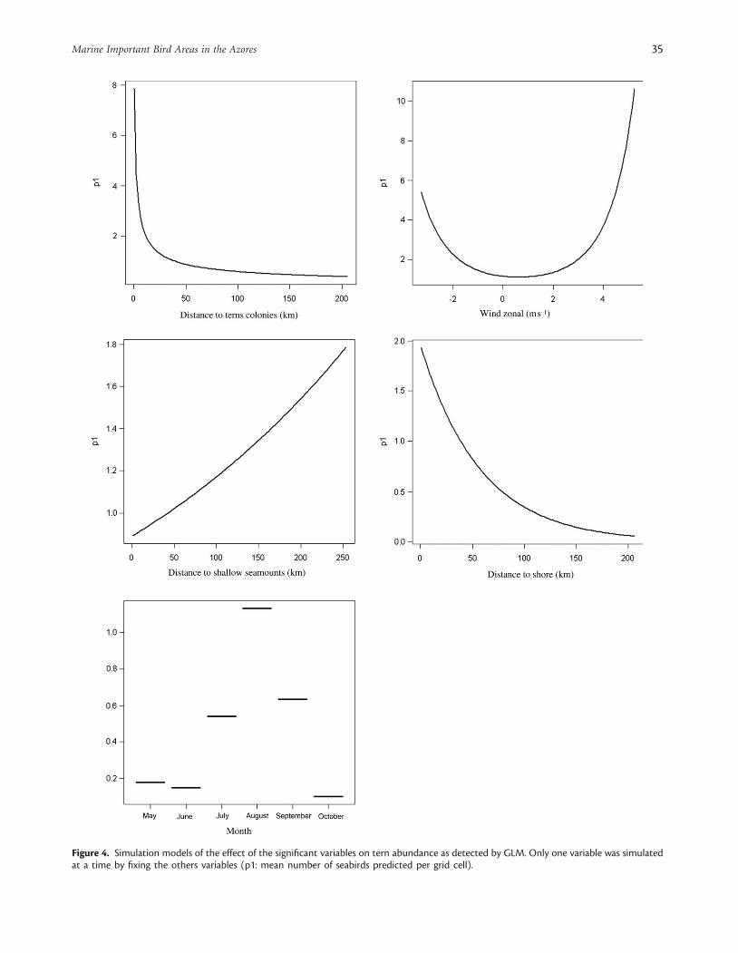
Figure 4. Simulation models of the effect of the significant variables on tern abundance as detected by GLM. Only one variable was simulatedat a time by fixing the others variables (p1: mean number of seabirds predicted per grid cell).

Marine Important Bird Areas in the Azores 35

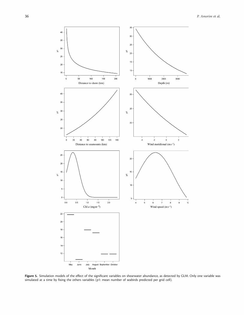
Figure 5. Simulation models of the effect of the significant variables on shearwater abundance, as detected by GLM. Only one variable wassimulated at a time by fixing the others variables (p1: mean number of seabirds predicted per grid cell).

36 P. Amorim et al.

resorted to pooling the shearwater data and using the modelresults from the combined onshore–offshore observations.

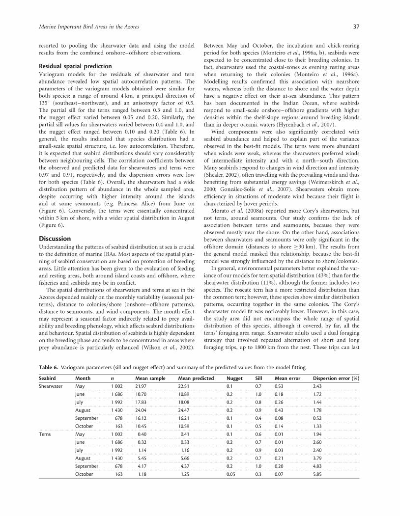
Residual spatial predictionVariogram models for the residuals of shearwater and ternabundance revealed low spatial autocorrelation patterns. Theparameters of the variogram models obtained were similar forboth species: a range of around 4 km, a principal direction of1358 (southeast–northwest), and an anisotropy factor of 0.5.The partial sill for the terns ranged between 0.3 and 1.0, andthe nugget effect varied between 0.05 and 0.20. Similarly, thepartial sill values for shearwaters varied between 0.4 and 1.0, andthe nugget effect ranged between 0.10 and 0.20 (Table 6). Ingeneral, the results indicated that species distribution had asmall-scale spatial structure, i.e. low autocorrelation. Therefore,it is expected that seabird distributions should vary considerablybetween neighbouring cells. The correlation coefficients betweenthe observed and predicted data for shearwaters and terns were0.97 and 0.91, respectively, and the dispersion errors were lowfor both species (Table 6). Overall, the shearwaters had a widedistribution pattern of abundance in the whole sampled area,despite occurring with higher intensity around the islandsand at some seamounts (e.g. Princesa Alice) from June on(Figure 6). Conversely, the terns were essentially concentratedwithin 5 km of shore, with a wider spatial distribution in August(Figure 6).

DiscussionUnderstanding the patterns of seabird distribution at sea is crucialto the definition of marine IBAs. Most aspects of the spatial plan-ning of seabird conservation are based on protection of breedingareas. Little attention has been given to the evaluation of feedingand resting areas, both around island coasts and offshore, wherefisheries and seabirds may be in conflict.

The spatial distributions of shearwaters and terns at sea in theAzores depended mainly on the monthly variability (seasonal pat-terns), distance to colonies/shore (onshore–offshore patterns),distance to seamounts, and wind components. The month effectmay represent a seasonal factor indirectly related to prey avail-ability and breeding phenology, which affects seabird distributionsand behaviour. Spatial distribution of seabirds is highly dependenton the breeding phase and tends to be concentrated in areas whereprey abundance is particularly enhanced (Wilson et al., 2002).

Between May and October, the incubation and chick-rearingperiod for both species (Monteiro et al., 1996a, b), seabirds wereexpected to be concentrated close to their breeding colonies. Infact, shearwaters used the coastal-zones as evening resting areaswhen returning to their colonies (Monteiro et al., 1996a).Modelling results confirmed this association with nearshorewaters, whereas both the distance to shore and the water depthhave a negative effect on their at-sea abundance. This patternhas been documented in the Indian Ocean, where seabirdsrespond to small-scale onshore–offshore gradients with higherdensities within the shelf-slope regions around breeding islandsthan in deeper oceanic waters (Hyrenbach et al., 2007).

Wind components were also significantly correlated withseabird abundance and helped to explain part of the varianceobserved in the best-fit models. The terns were more abundantwhen winds were weak, whereas the shearwaters preferred windsof intermediate intensity and with a north–south direction.Many seabirds respond to changes in wind direction and intensity(Shealer, 2002), often travelling with the prevailing winds and thusbenefiting from substantial energy savings (Weimerskirch et al.,2000; Gonzalez-Solıs et al., 2007). Shearwaters obtain moreefficiency in situations of moderate wind because their flight ischaracterized by hover periods.

Morato et al. (2008a) reported more Cory’s shearwaters, butnot terns, around seamounts. Our study confirms the lack ofassociation between terns and seamounts, because they wereobserved mostly near the shore. On the other hand, associationsbetween shearwaters and seamounts were only significant in theoffshore domain (distances to shore �30 km). The results fromthe general model masked this relationship, because the best-fitmodel was strongly influenced by the distance to shore/colonies.

In general, environmental parameters better explained the var-iance of our models for tern spatial distribution (43%) than for theshearwater distribution (11%), although the former includes twospecies. The roseate tern has a more restricted distribution thanthe common tern; however, these species show similar distributionpatterns, occurring together in the same colonies. The Cory’sshearwater model fit was noticeably lower. However, in this case,the study area did not encompass the whole range of spatialdistribution of this species, although it covered, by far, all theterns’ foraging area range. Shearwater adults used a dual foragingstrategy that involved repeated alternation of short and longforaging trips, up to 1800 km from the nest. These trips can last

. . . . . . . . . . . . . . . . . . . . . . . . . . . . . .

. . . . . . . . . . . . . . . . . . . . . . . . . . . . .. . . . . . . . . . . . . . . . . . . .. . . . . . . . . . . . . . . . . . . . . . . . . . . . . . . . . . .. . . . . . . . . . . . . . . . . . . . . . . . . . . . . . . . . . . . . . . .. . . . . . . . . . . . . . . . . . . . . . . .. . . . . . . . . . . . . . . .. . . . . . . . . . . . . . . . . . . . . . . . . . . . . . .. . . . . . . . . . . . . . . . . . . . . . . . . . . . . . . . . . . . . .

. . . . . . . . . . . . . . . . . . . . . . . . . . . . .. . . . . . . . . . . . . . . . . . . .. . . . . . . . . . . . . . . . . . . . . . . . . . . . . . . . . . .. . . . . . . . . . . . . . . . . . . . . . . . . . . . . . . . . . . . . . . .. . . . . . . . . . . . . . . . . . . . . . . .. . . . . . . . . . . . . . . .. . . . . . . . . . . . . . . . . . . . . . . . . . . . . . .. . . . . . . . . . . . . . . . . . . . . . . . . . . . . . . . . . . . . .

. . . . . . . . . . . . . . . . . . . . . . . . . . . . .. . . . . . . . . . . . . . . . . . . .. . . . . . . . . . . . . . . . . . . . . . . . . . . . . . . . . . .. . . . . . . . . . . . . . . . . . . . . . . . . . . . . . . . . . . . . . . .. . . . . . . . . . . . . . . . . . . . . . . .. . . . . . . . . . . . . . . .. . . . . . . . . . . . . . . . . . . . . . . . . . . . . . .. . . . . . . . . . . . . . . . . . . . . . . . . . . . . . . . . . . . . .

. . . . . . . . . . . . . . . . . . . . . . . . . . . . .. . . . . . . . . . . . . . . . . . . .. . . . . . . . . . . . . . . . . . . . . . . . . . . . . . . . . . .. . . . . . . . . . . . . . . . . . . . . . . . . . . . . . . . . . . . . . . .. . . . . . . . . . . . . . . . . . . . . . . .. . . . . . . . . . . . . . . .. . . . . . . . . . . . . . . . . . . . . . . . . . . . . . .. . . . . . . . . . . . . . . . . . . . . . . . . . . . . . . . . . . . . .

. . . . . . . . . . . . . . . . . . . . . . . . . . . . .. . . . . . . . . . . . . . . . . . . .. . . . . . . . . . . . . . . . . . . . . . . . . . . . . . . . . . .. . . . . . . . . . . . . . . . . . . . . . . . . . . . . . . . . . . . . . . .. . . . . . . . . . . . . . . . . . . . . . . .. . . . . . . . . . . . . . . .. . . . . . . . . . . . . . . . . . . . . . . . . . . . . . .. . . . . . . . . . . . . . . . . . . . . . . . . . . . . . . . . . . . . .

. . . . . . . . . . . . . . . . . . . . . . . . . . . . .. . . . . . . . . . . . . . . . . . . .. . . . . . . . . . . . . . . . . . . . . . . . . . . . . . . . . . .. . . . . . . . . . . . . . . . . . . . . . . . . . . . . . . . . . . . . . . .. . . . . . . . . . . . . . . . . . . . . . . .. . . . . . . . . . . . . . . .. . . . . . . . . . . . . . . . . . . . . . . . . . . . . . .. . . . . . . . . . . . . . . . . . . . . . . . . . . . . . . . . . . . . .

. . . . . . . . . . . . . . . . . . . . . . . . . . . . .. . . . . . . . . . . . . . . . . . . .. . . . . . . . . . . . . . . . . . . . . . . . . . . . . . . . . . .. . . . . . . . . . . . . . . . . . . . . . . . . . . . . . . . . . . . . . . .. . . . . . . . . . . . . . . . . . . . . . . .. . . . . . . . . . . . . . . .. . . . . . . . . . . . . . . . . . . . . . . . . . . . . . .. . . . . . . . . . . . . . . . . . . . . . . . . . . . . . . . . . . . . .

. . . . . . . . . . . . . . . . . . . . . . . . . . . . .. . . . . . . . . . . . . . . . . . . .. . . . . . . . . . . . . . . . . . . . . . . . . . . . . . . . . . .. . . . . . . . . . . . . . . . . . . . . . . . . . . . . . . . . . . . . . . .. . . . . . . . . . . . . . . . . . . . . . . .. . . . . . . . . . . . . . . .. . . . . . . . . . . . . . . . . . . . . . . . . . . . . . .. . . . . . . . . . . . . . . . . . . . . . . . . . . . . . . . . . . . . .

. . . . . . . . . . . . . . . . . . . . . . . . . . . . .. . . . . . . . . . . . . . . . . . . .. . . . . . . . . . . . . . . . . . . . . . . . . . . . . . . . . . .. . . . . . . . . . . . . . . . . . . . . . . . . . . . . . . . . . . . . . . .. . . . . . . . . . . . . . . . . . . . . . . .. . . . . . . . . . . . . . . .. . . . . . . . . . . . . . . . . . . . . . . . . . . . . . .. . . . . . . . . . . . . . . . . . . . . . . . . . . . . . . . . . . . . .

. . . . . . . . . . . . . . . . . . . . . . . . . . . . .. . . . . . . . . . . . . . . . . . . .. . . . . . . . . . . . . . . . . . . . . . . . . . . . . . . . . . .. . . . . . . . . . . . . . . . . . . . . . . . . . . . . . . . . . . . . . . .. . . . . . . . . . . . . . . . . . . . . . . .. . . . . . . . . . . . . . . .. . . . . . . . . . . . . . . . . . . . . . . . . . . . . . .. . . . . . . . . . . . . . . . . . . . . . . . . . . . . . . . . . . . . .

. . . . . . . . . . . . . . . . . . . . . . . . . . . . .. . . . . . . . . . . . . . . . . . . .. . . . . . . . . . . . . . . . . . . . . . . . . . . . . . . . . . .. . . . . . . . . . . . . . . . . . . . . . . . . . . . . . . . . . . . . . . .. . . . . . . . . . . . . . . . . . . . . . . .. . . . . . . . . . . . . . . .. . . . . . . . . . . . . . . . . . . . . . . . . . . . . . .. . . . . . . . . . . . . . . . . . . . . . . . . . . . . . . . . . . . . .

Table 6. Variogram parameters (sill and nugget effect) and summary of the predicted values from the model fitting.

Seabird Month n Mean sample Mean predicted Nugget Sill Mean error Dispersion error (%)

Shearwater May 1 002 21.97 22.51 0.1 0.7 0.53 2.43

June 1 686 10.70 10.89 0.2 1.0 0.18 1.72

July 1 992 17.83 18.08 0.2 0.8 0.26 1.44

August 1 430 24.04 24.47 0.2 0.9 0.43 1.78

September 678 16.12 16.21 0.1 0.4 0.08 0.52

October 163 10.45 10.59 0.1 0.5 0.14 1.33

Terns May 1 002 0.40 0.41 0.1 0.6 0.01 1.94

June 1 686 0.32 0.33 0.2 0.7 0.01 2.60

July 1 992 1.14 1.16 0.2 0.9 0.03 2.40

August 1 430 5.45 5.66 0.2 0.7 0.21 3.79

September 678 4.17 4.37 0.2 1.0 0.20 4.83

October 163 1.18 1.25 0.05 0.3 0.07 5.85

Marine Important Bird Areas in the Azores 37

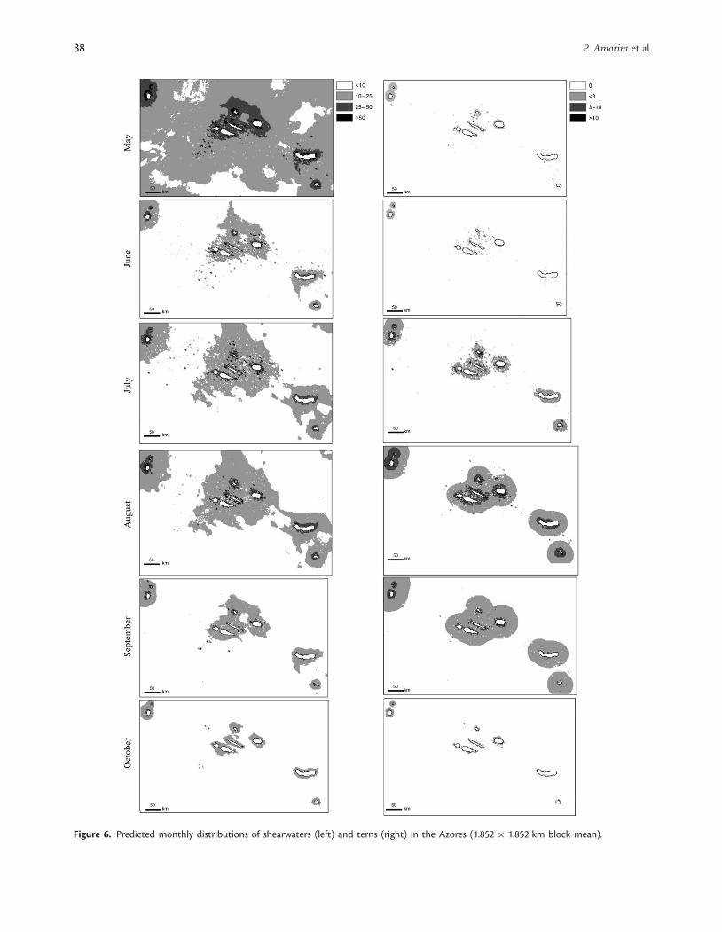
Figure 6. Predicted monthly distributions of shearwaters (left) and terns (right) in the Azores (1.852 � 1.852 km block mean).

38 P. Amorim et al.

for several days (mean 9 d; +2.7 s.d.) and occurred in areas ofhigher productivity north of the Azores EEZ, whereas short tripswere evenly distributed around breeding colonies (Magalhaeset al., 2008). However, the variance explained by this type ofmodel is within common values for such studies. For example,Louzao et al. (2006) used a similar approach to characterize thepresence or absence of the Balearic shearwater (Puffinus maurita-nicus) and developed a model explaining 21% of the observedvariability. Another reason for the low variability explained bythe GLM might be related to data collection, because our samplingwas not spatially random but was heavily influenced by the beha-viour of the tuna fishing fleet. Usually, the tuna fleet tends tooperate around the islands and in some well-known seamounts(e.g. Princesa Alice). Additionally, the data do not includeseabird behaviour, which could also enhance the effect of colonylocation because birds travelling between the colonies and foragingareas would be seen more often close to the colony. Hence, tounderstand the behaviour and distribution of the Cory’s shear-water at sea better, it would be necessary to widen the investigationto include their whole geographic distribution range, by addition-ally compiling data on seabird distribution and behaviour duringthe entire period that they are present in the Azores, includingthe post-breeding winter dispersal from breeding colonies. Inparticular, movement data collected with geolocation dataloggers may be a good complement to traditional census andcould furnish detailed information on the offshore foraging areas.

In summary, the geostatistical methods used in this study,incorporating environmental parameters, contributed to a betterunderstanding of the spatial at-sea distribution of Cory’s shear-water and tern populations in the Azores coastal and offshoreregions. The predictive maps that result from this study are animportant tool for defining marine IBAs in the Azores. Monthlymaps (May–October) of predicted shearwater and tern distri-bution in the Azores were produced. Terns appeared mostlyconcentrated within 5 km of shore, with a broad distribution inAugust when most tern chicks have fledged (Monteiro et al.,1996b), resulting in a wider tern foraging range. Cory’s shearwaterswere evenly distributed in the whole study area, although theyoccurred in larger numbers around the islands from June on,coinciding with the egg-laying and incubation period (Monteiroet al., 1996b). The results of this study (Figure 6) revealed higherconcentrations of shearwaters and/or terns in Corvo, Flores, thenorth and west coasts of Faial, the northwest shore of Pico, theeast and west extremes of Sao Jorge, Graciosa, the east coast ofTerceira, Sao Miguel (Ilheu de Vila Franca), and Santa Maria.These data will be compared with recent census data and data-logger information to help define the future coastal IBAs. Theareas around the seamounts (Princesa Alice, Formigas, andDollabarat; Figure 6) were also preferred areas of Cory’s shearwateroccurrence. These seamounts should be considered as potentialoffshore IBAs.

Our findings demonstrate that, at an archipelago level, thewaters surrounding breeding colonies are the most relevant interms of seabird concentrations. However, these areas wereexcluded from the Natura 2000 SPAs that were declared for theapplication of the Birds Directive (79/409/ECC). In particular,these areas pose potential conflicts between seabird protectionand fisheries. Small pelagic fish, such as jack mackerel(Trachurus picturatus) and young black-spot sea bream (Pagellusbogaraveo), are caught seasonally close to shore by the Azoreantuna fleet to be used as live bait. The shore areas are also where

greater abundances of shearwaters and terns are found duringthe breeding season. Therefore, marine protected areas encom-passing the waters surrounding seabird breeding areas should beencouraged, at least during the breeding season or when thepursuit of commercial fisheries for small pelagic fish mayoverlap temporally with dense concentrations of resting orforaging seabirds. However, to improve the spatial and temporaldefinition of MPAs, further studies are certainly required, e.g. toquantify the spatial overlap between live-bait fishing and seabirddistributions, to infer potential competition strategies for thesame resources (e.g. species and size classes targeted), or toevaluate possible negative impacts on seabirds populations (e.g.lowered reproductive success).

AcknowledgementsThis work was funded by the project EU/LIFE-IBAs (LIF04NAT/PT/000213): Important Areas for Marine Birds in Portugal.Biological data used in this study were obtained from the AzoresFisheries Observers Programme (POPA), which is funded mainlyby the Regional Directorate of Fisheries of the Azores. Between2002 and 2006, POPA was also funded by ORPAM – InterREG:MAC/4.2/A1 (part FEDER). Satellite data were obtained fromthe HAZO station in the Azores and from NASA/GSFC. Thesedata were processed and distributed by the OceanographySection at the Department of Oceanography and Fisheries of theUniversity of the Azores (DOP/UAc), and funded through scien-tific projects RAA-SRAPA/DRP-DETRA and OPALINA (PDCTE/CTA/49965/2003). We also thank the IFREMER Centre ERSd’Archivage et de Traitement (CERSAT) for providing onlinedata on wind components. The presentation of this work at theEuropean Symposium on Marine Protected Areas was funded bythe Azores Regional Directorate of Science and Technology(DRCT). We are also grateful to A. Bio for assistance helpingwith data analysis and to J. Bried, V. Neves, M. Magalhaes, andthe two anonymous referees for their comments, which greatlyimproved this paper. Research at IMAR-DOP/UAc (UI&D #531and ISR LA#9) is funded by FCT and DRCT/Azores throughpluri-annual and programmatic funding schemes (part FEDER).TM acknowledges support from the Fundacao para a Ciencia eTecnologia (Portugal, SFRH//BPD/27007/2006).

ReferencesAinley, D. G., Spear, L. B., Tynan, C. T., Barth, J. A., Pierce, S. D., Ford,

R. G., and Cowles, T. J. 2005. Physical and biological variablesaffecting seabird distributions during the upwelling season of thenorthern California Current. Deep Sea Research II, 52: 123–143.

Ballance, L. T., and Pitman, R. L. 1999. Foraging ecology of tropicalseabirds. In Proceedings of the 22nd International OrnithologicalCongress, Durban, pp. 2057–2071. Ed. by N. Adams, and R.Slotow. BirdLife South Africa, Johannesburg.

Ballance, L. T., Pitman, R. L., and Fiedler, P. C. 2006. Oceanographicinfluences on seabirds and cetaceans of the eastern tropical Pacific:a review. Progress in Oceanography, 69: 360–390.

Begg, G. S., and Reid, J. B. 1997. Spatial variation in seabird density at ashallow sea tidal mixing front in the Irish Sea. ICES Journal ofMarine Science, 54: 552–565.

Bio, A. M. F. 2000. Does vegetation suit our models? Data and modelassumptions and the assessment of species distribution in space.Nederlandse Geografische Studies 265. Utrecht.

BirdLife International. 2004. Birds in Europe: Population Estimates,Trends and Conservation Status. BirdLife International, BirdLifeConservation Series, 12. Cambridge, UK. 374 pp.

Marine Important Bird Areas in the Azores 39

Dalgaard, P. 2002. Introductory Statistics with R. Springer-Verlag,New York. 267 pp.

Feio, R., Dias, L., and Machete, M. 2005. Manual do Observador.Series internas do DOP. 88 pp. www.popaobserver.org.

Figueiredo, M., Martins, A., Castellanos, P., Mendonca, A., Macedo,L., Rodrigues, M., Lafon, V., et al. 2004. HAZO: a softwarepackage for automated AVHRR and SeaWiFS acquisition andprocessing. Arquivos do DOP, Serie Relatorios Internos, 3/2004.92 pp.

Garthe, S. 1997. Influence of hydrography, fishing activity, and colonylocation on summer seabird distribution in the south-easternNorth Sea. ICES Journal of Marine Science, 54: 566–577.

Gonzalez-Solıs, J., Croxall, J. P., Oro, D., and Ruiz, X. 2007.Trans-equatorial migration and mixing in the wintering areas ofa pelagic seabird. Frontiers in Ecology and the Environment, 5:297–301.

Hunt, G. L., Mehlum, F., Russell, R. W., Irons, D., Decker, M. B., andBecker, P. H. 1999. Physical processes, prey abundance, and theforaging ecology of seabirds. In Proceedings of the 22ndInternational Ornithological Congress, Durban, pp. 2040–2056.Ed. by N. Adams, and R. Slotow. BirdLife South Africa,Johannesburg.

Hunt, G. L., and Schneider, D. C. 1987. Scale dependent processesin the physical and biological environment of seabirds. InThe Feeding Ecology of Seabirds and their Role in MarineEcosystems, pp. 7–41. Ed. by J. P. Croxall. Cambridge UniversityPress, Cambridge. 416 pp.

Hyrenbach, K. D., Veit, R. R., Weimerskirch, H., and Hunt, G. L. 2006.Seabird associations with mesoscale eddies: the subtropical IndianOcean. Marine Ecology Progress Series, 324: 271–279.

Hyrenbach, K. D., Veit, R. R., Weimerskirch, H., Metzl, N., and Hunt,G. L. 2007. Community structure across a large-scale oceanproductivity gradient: marine bird assemblages of the southernIndian Ocean. Deep Sea Research I, 54: 1129–1145.

Lourenco, N., Miranda, J. M., Luis, J. F., Ribeiro, A., Mendes Vıtor,L. A., Madeira, J., et al. 1998. Morpho-tectonic analysis of theAzores volcanic plateau from a new bathymetric compilation ofthe area. Marine Geophysical Researches, 20: 141–156.

Louzao, M., Hyrenbach, K. D., Arcos, J. M., Abello, P., de Sola, L. G.,and Oro, D. 2006. Oceanographic habitat of an endangeredMediterranean procellariiform: implications for marine protectedareas. Ecological Applications, 16: 1683–1695.

Machete, M., and Santos, R. S. 2007. Azores Fisheries ObserverProgram (POPA): a case study of the multidisciplinary use ofobserver data. In Proceedings of the 5th International FisheriesObserver Conference, Victoria, British Columbia, Canada, 15–18May 2007, pp. 114–116. Ed. by T. A. McVea, and S. J. Kennelly.NSW Department of Primary Industries, Cronulla FisheriesResearch Centre of Excellence, Cronulla, Australia. 412 pp.

Magalhaes, M. S., Santos, R. S., and Hamer, K. C. 2008. Dual-foragingof Cory’s shearwaters in the Azores: feeding locations, behaviourat-sea and implications for food provisioning of chicks. MarineEcology Progress Series, 359: 283–293.

Monteiro, L. R. 2000. The Azores. In Important Bird Areas in Europe:Priority Sites for Conservation. 2: Southern Europe, pp. 463–472.Ed. by M. F. Heath, and M. I. Evans. BirdLife International BirdLifeConservation Series, 8. Cambridge, UK. 791 pp.

Monteiro, L. R., Ramos, J. A., and Furness, R. W. 1996a. Past andpresent status and conservation of the seabirds breeding in theAzores Archipelago. Biological Conservation, 78: 319–328.

Monteiro, L. R., Ramos, J. A., Furness, R. W., and Del Nevo, A. J.1996b. Movements, morphology, breeding, molt, diet andfeeding of seabirds in the Azores. Colonial Waterbirds, 19: 82–97.

Morato, T., Machete, M., Kitchingman, A., Tempera, F., Lai, S.,Menezes, G., Pitcher, T. J., et al. 2008b. Abundance and distri-bution of seamounts in the Azores. Marine Ecology ProgressSeries, 357: 17–21.

Morato, T., Varkey, D. A., Damaso, C., Machete, M., Santos, M.,Prieto, R., Santos, R. S., et al. 2008a. Evidence of seamount effecton aggregating visitors. Marine Ecology Progress Series, 357:23–32.

Neves, V. 2007. Azores 2007 Tern Census. Arquivos do DOP, SerieEstudos, 4/2007. 21 pp.

Pebesma, E. J. 2004. Multivariate geostatistics in S: the gstat package.Computers and Geosciences, 30: 683–691.

Pebesma, E. J., Duin, R. N. M., and Burrough, P. A. 2005. Mapping seabird densities over the North Sea: spatially aggregated estimatesand temporal changes. Environmetrics, 16: 573–587.

Santos, R. S., Hawkins, S. J., Monteiro, L. R., Alves, M., and Isidro, E. J.1995. Marine research, resources and conservation in the Azores.Aquatic Conservation. Marine and Freshwater Ecosystems, 5:311–354.

Schneider, D. C. 1997. Habitat selection by marine birds in relation towater depth. Ibis, 139: 175–178.

Shealer, D. A. 2002. Foraging behaviour and food of seabirds. InBiology of Marine Birds, pp. 137–178. Ed. by E. A. Schreiber,and J. Burger. CRC Press, Boca Raton, FL. 744 pp.

Spear, L. B., and Ainley, D. G. 1998. Morphological differences relativeto ecological segregation in petrels (family: Procellariidae) of theSouthern Ocean and Tropical Pacific. Auk, 115: 1017–1033.

Suryan, R. M., Sato, F., Balogh, G. R., Hyrenbach, K. D., Sievert, P. R.,and Ozaki, K. 2006. Foraging destinations and marine habitat useof short-tailed albatrosses. A multi-scale approach using first-passage time analysis. Deep Sea Research II, 53: 370–386.

Valavanis, V. D., Katara, I., and Palialexis, A. 2005. Marine GIS: identi-fication of mesoscale oceanic thermal fronts. International Journalof Geographical Information Science, 19: 1131–1147.

Weimerskirch, H., Guionnet, T., Martin, J., Shaffer, S. A., and Costa,D. P. 2000. Fast and fuel efficient? Optimal use of wind by flyingalbatrosses. Proceedings of the Royal Society of London, Series B,267: 1869–1874.

Wilson, R. P., Gremillet, D., Syder, J., Kierspel, M. A. M., Garthe, S.,Weimerskirch, H., Schafer-Neth, C., et al. 2002. Remote-sensingsystems and seabirds: their use, abuse and potential for measuringmarine environmental variables. Marine Ecology Progress Series,228: 241–261.

Yen, P. P. W., Sydeman, W. J., Bograd, S. J., and Hyrenbach, K. D. 2006.Spring-time distributions of migratory marine birds in thesouthern California Current: oceanic eddy associations andcoastal habitat hotspots over 17 years. Deep Sea Research II, 53:399–418.

Yen, P. P. W., Sydeman, W. J., and Hyrenbach, K. 2004. Marine birdand cetacean associations with bathymetric habitats and shallow-water topographies: implications for trophic transfer and conserva-tion. Journal of Marine Systems, 50: 79–99.

doi:10.1093/icesjms/fsn175

40 P. Amorim et al.