Spatial regression modeling for compositional data with many zeros Thomas J. Leininger Alan E. Gelfand Jenica M. Allen John A. Silander, Jr. * April 13, 2013 Abstract Compositional data analysis considers vectors of nonnegative-valued variables sub- ject to a unit-sum constraint. Our interest lies in spatial compositional data, in par- ticular, land use/land cover (LULC) data in the northeastern United States. Here, the observations are vectors providing the proportions of LULC types observed in each 3km × 3km grid cell, yielding order 10 4 cells. On the same grid cells, we have an additional compositional dataset supplying forest fragmentation proportions. Poten- tially useful and available covariates include elevation range, road length, population, median household income, and housing levels. We propose a spatial regression model that is also able to capture flexible depen- dence among the components of the observation vectors at each location as well as spatial dependence across the locations of the simplex-restricted measurements. A key * Thomas J. Leininger is a Ph.D. candidate (Email: [email protected]) and Alan E. Gelfand is a professor (E-mail: [email protected]), Department of Statistical Science, Duke University, Box 90251, Durham, NC 27708-0251, USA. Jenica M. Allen is an assistant professor in residence (Email: [email protected]) and John A. Silander, Jr., is a professor (Email: [email protected]), De- partment of Ecology and Evolutionary Biology, University of Connecticut, 75 North Eagleville Road, Unit 3043, Storrs, Connecticut 06269, USA. The authors thank Daniel Civco and James Hurd for acquiring and processing the data and Adam Wilson and Corey Merow for useful conversations. This work was supported in part by USDA-NRI 2008-003237. 1

Welcome message from author
This document is posted to help you gain knowledge. Please leave a comment to let me know what you think about it! Share it to your friends and learn new things together.
Transcript
Spatial regression modeling for compositional data with
many zeros
Thomas J. Leininger Alan E. Gelfand Jenica M. Allen
John A. Silander, Jr. ∗
April 13, 2013
Abstract
Compositional data analysis considers vectors of nonnegative-valued variables sub-
ject to a unit-sum constraint. Our interest lies in spatial compositional data, in par-
ticular, land use/land cover (LULC) data in the northeastern United States. Here,
the observations are vectors providing the proportions of LULC types observed in each
3km × 3km grid cell, yielding order 104 cells. On the same grid cells, we have an
additional compositional dataset supplying forest fragmentation proportions. Poten-
tially useful and available covariates include elevation range, road length, population,
median household income, and housing levels.
We propose a spatial regression model that is also able to capture flexible depen-
dence among the components of the observation vectors at each location as well as
spatial dependence across the locations of the simplex-restricted measurements. A key
∗Thomas J. Leininger is a Ph.D. candidate (Email: [email protected]) and Alan E. Gelfandis a professor (E-mail: [email protected]), Department of Statistical Science, Duke University, Box90251, Durham, NC 27708-0251, USA. Jenica M. Allen is an assistant professor in residence (Email:[email protected]) and John A. Silander, Jr., is a professor (Email: [email protected]), De-partment of Ecology and Evolutionary Biology, University of Connecticut, 75 North Eagleville Road, Unit3043, Storrs, Connecticut 06269, USA. The authors thank Daniel Civco and James Hurd for acquiring andprocessing the data and Adam Wilson and Corey Merow for useful conversations. This work was supportedin part by USDA-NRI 2008-003237.
1
issue is the high incidence of observed zero proportions for the LULC dataset, requiring
incorporation of local point masses at 0. We build a hierarchical model prescribing a
power scaling first stage and using latent variables at the second stage with spatial
structure for these variables supplied through a multivariate CAR specification. Anal-
yses for the LULC and forest fragmentation data illustrate the interpretation of the
regression coefficients and the benefit of incorporating spatial smoothing.
Keywords: areal data; conditionally autoregressive model; continuous ranked probabil-
ity score; hierarchical modeling; Markov Chain Monte Carlo
1 Introduction
Compositional data analysis is concerned with inference for data in the form of vectors
of nonnegative observations that are subject to a constant-sum constraint (without loss of
generality, a unit-sum constraint). This defines, for a D-dimensional vector Y, a sample
space referred to as the simplex SD−1 = Y : 0 ≤ Yk ≤ 1, YT1 = 1 (Aitchison, 1986).
One setting where compositional data arises is in the analysis of proportions of land cover
composing geographical regions. Each observation is a vector of proportions, with entries
specifying the proportion of that region covered by a specific land cover category. Early work
ignored these constraints and applied standard multivariate analysis. However, much effort
has been devoted in the last 30 years to understanding the nature of such data and developing
appropriate methods for their analysis, as discussed in, e.g., Aitchison and Egozcue (2005).
The contribution of this paper is to present a novel model specification for spatial re-
gression on compositional data. The novelty addresses the issue that, for our observation
vectors, components take on the value 0 sufficiently often to require point masses at 0. We
view a 0 entry for a component of a vector at a location as arising at random, rather than
as an essential zero, i.e., an entry that must be 0 for that component at that location. It is
also possible that a zero value is observed due to rounding or to the true value being below
2

some minimum detection level. Observed zeros arise frequently with nominal categorical
data if we seek to avoid collapsing and aggregating of categories. Current methods lack
ease of implementation and/or suitable interpretation when having to handle zero values,
complicating regression and inference. A model that permits point masses to explain the
zero values becomes useful in this context. Moreover, the compositional data vectors are
each associated with a distinct areal unit and compositions in neighboring cells are expected
to be similar. As a result, we first present the non-spatial case but readily move to the
spatial setting through introduction of spatial random effects. In fact, with dynamic spatial
compositional data, spatio-temporal random effects could also be introduced. The model is
specified hierarchically, where fitting is done within a Bayesian framework.
One setting where compositional data arises is in the analysis of proportions of land
cover types comprising geographical units. We illustrate the compositional data regression
problem using data consisting of the proportions of a set of land use/land cover (LULC)
classes at the scale of 3km × 3km grid cells over a region covering the northeastern United
States, resulting in n = 19, 210 cells. Individual proportions are often zero. For instance,
many cells in rural areas exhibit a high concentration of forest but no urbanization. In fact,
for the Developed classification in our dataset, zero values occur in 21% of the cells. Potential
explanatory variables for the regression modeling are drawn from US Census data along with
measurements of road length and elevation change. The observations are also collected at
four different times, providing the possibility of modeling change in land use/land cover
over time. A second setting considered is that of forest fragmentation. Here, working again
in the northeastern United States, grid cells describe a forest fragmentation process which
yields the classifications: Patch, Edge, Perforated, or Core forest as well as Other. Potential
explanatory variables for regression modeling include the same covariates as above.
3
2 Previous work
While the Dirichlet distribution might seem a natural choice for modeling data with a unit-
sum constraint, the implicit negative pairwise correlations between all components can be
overly restrictive. Additionally, the fact that the mean of a Dirichlet distribution determines
the covariance structure is also restrictive. Compositional data are therefore often analyzed
using transformations such as the additive logratio (alr) transformation (Aitchison, 1986) or
isometric logratio (ilr) transformation (Egozcue et al., 2003), whence standard multivariate
methods can then be applied to the transformed data. Model fitting software for both
transformations is available, e.g., using CoDaPack or the compositions package (van den
Boogaart and Tolosana-Delgado, 2008) in R (R Core Team, 2012).
One shortcoming of these methods is that they do not allow zero values in the compo-
nents. Handling rounded zeros can be done by assigning a pre-determined small value to the
component or through an imputation algorithm (Fry et al., 2000; Martın-Fernandez et al.,
2003). However, adding a small value seems arbitrary and may not be satisfying when there
are numerous zero values.
Scealy and Welsh (2011), building on work by Stephens (1982), employ a square-root
transformation to convert the compositional data to directional data, where the occurrence
of zeros is no longer an issue. They then specify the Kent distribution (Kent, 1982), a distri-
bution defined on the hypersphere, to provide regression models. Butler and Glasbey (2009)
handle zeros by introducing a latent Gaussian variable Z, which maps the data from the
simplex to the unit hyperplane HD = W ∈ RD : WT1 = 1. They use the transforma-
tion Y = g(W) which minimizes the squared Euclidean distance (Y −W)T (Y −W). The
truncation imposed by their method enables a point mass at 0. However, accommodating
D > 3 seems very challenging. Stewart and Field (2010) model zero values separately using
mixture specifications. Conditional models are specified given the set of nonzero components
and usually take the form of a multiplicative logistic (possibly skewed) normal distribution.
4

Salter-Townshend and Haslett (2006) suggest a one-stage approach representing compo-
nents of Y in the form Yk = max(0, Zk)/(∑D
k′=1 max(0, Zk′)), where Zk is a latent random
variable that is presumed normally distributed. The function max(0, Zk) takes the maxi-
mum between 0 and Zk, which ensures that negative values of Yk are not allowed by mapping
negative values of Zk to a point mass at Yk = 0. The use of a Box-Cox transformation from
the data Y to transformed data Z using Zk = ((Yk/YD)γ − 1)/γ, for k = 1, . . . , D − 1, with
a (possibly component-specific) scaling parameter γ is considered in Aitchison (1986), Fry
et al. (2000), and Tsagris et al. (2011). This approach requires that one component, taken
here to be the last component, YD, is always nonzero so it can serve as a baseline. Our
proposed method, building on these approaches, uses a simple transformation by employing
a latent Gaussian variable, allowing direct incorporation of regression and spatial effects.
We create a point mass at 0 similar to the Butler-Glasbey and Stewart-Field models, but
through a comparison of the components to a baseline, similar to the alr transformation.
There has been some previous spatial compositional data work. Billheimer et al. (1997)
studied the composition of benthic species across sample sites. Using the alr transforma-
tion to Z = alr(Y), they modeled Z with regression and random spatial effects, the latter
being modeled with a multivariate spatial conditional autoregressive model (Mardia, 1988).
Tjelmeland and Lund (2003) extended the logistic normal distribution, incorporating Gaus-
sian processes to model spatial structure. Similarly, Haslett et al. (2006) introduce a spatial
process using a linear variogram approach, incorporating spatial effects in a two-stage model.
When working with data on, for example, a regular 3km grid, one customarily adopts
areal data spatial models. Conditionally autoregressive (CAR) models, dating to Besag
(1974), are a common choice. Multivariate CAR (MCAR) specifications (Mardia, 1988) are
required for multivariate observations at areal units. Further development is provided in
Gelfand and Vounatsou (2003). Coregionalizaton, that is, linear transformation of indepen-
dent univariate CAR processes, is considered in Gelfand et al. (2004).
The format of the remainder of the paper is as follows. In Section 3 we introduce the
5
compositional datasets used to investigate land use/land cover and forest fragmentation
changes in the northeastern United States. In Section 4, we present a compositional model
that allows point masses at zero and discuss properties of the model along with model fitting
and inference. In sections 5 and 6 we present analyses with simulated and real data to
highlight the usefulness and performance of our proposed model. We offer a brief summary
and possibilities for future work in Section 7.
3 Datasets
With the goal of studying changes in land use and land cover in the northeastern United
States, we analyze LULC data collected as part of the National Land Cover Dataset (NLCD)
(Fry et al., 2009) and the Coastal Change Analysis Program (CCAP) (National Oceanic and
Atmospheric Administration, 2006) from LANDSAT imagery at 30 meter resolution. Maps
generated from these satellite images describe the usage type of each 30 meter pixel and
provide a summary of the proportions of each LULC class within each of the 3km × 3km
grid cells, altogether a total of 19,210 grid cells. There are fourteen available LULC classes,
which we collapsed into four broader classes, as shown in Table 1. (Still, many zero values
are observed, as we quantify below.) The collapsing decisions were made in consultation
with ecologists involved in this project.
Explaining the observed proportions of these resulting classes illuminates the LULC
process. The data are available at four time periods: 1992, 1996, 2001, and 2005/2006
(hereafter called 2006). There was little observed change in the components over time; most
of cells showed less than 5% change from 1992 to 2006. Therefore, we do not consider
dynamics in LULC and focus on the most recent time period.
The Forest classification is of primary interest, with goals of better understanding rela-
tionships with other classes and identifying factors that explain forest cover variation across
the region. Forest fragmentation effects on invasive plant species is of special interest. Fig-
6

Table 1: New LULC classifications based on collapsing the original classes.
New Class Developed Crops and Grass Forest Other
Original High Intensity Developed Urban Grassland Deciduous Forest Scrub and ShrublandClasses Medium Intensity Developed Pastures and Grassland Evergreen Forest Open Water
Low Intensity Developed Crops Mixed Forest Emergent Wetland
Woody Wetland Barren Land
ure 1(a) shows, for each classification in the LULC data, the locations where there is an
observed zero proportion. The observed incidence of 0’s for each class is: Developed, 0.2102;
Crops/Grass, 0.0433; Other, 0.0006; Forest, 0.0014. Figure 1(a) emphasizes the need for a
model for LULC data that accommodates many 0’s.
Developed
Crops/Grass
Other
Forest
(a) 2006 LULC data
Patch
Edge
Perforated
Core
Other
(b) 2006 forest fragmentation data
Figure 1: The black dots mark the incidence of a zero value in the (a) 2006 LULC data and(b) 2006 forest fragmentation data.
Using a GIS tool (Parent and Hurd, 2010), the forest cover classes were divided into
subclasses of core, patch, perforated, and edge forest. These subclasses address the issue of
forest fragmentation. Core forest represents regions of forest that are a pre-specified distance
from any non-forest regions. Edge forest represents parts of the forest surrounding the core
forest. Patch forest represents small groups of forest that are too small to include any core
forest. Perforated forest accounts for any forest cover surrounding a non-forest clearing in the
7

midst of a larger forest region containing areas of core forest. Forest fragmentation occurs
as the core forest class decreases and the remaining classes increase.
For the forest fragmentation data, the proportions of zeros are: Patch, 0.0369; Edge,
0.0340; Perforated, 0.0216; Core, 0.0095; Other, 0. Figure 1(b) shows the locations of the
observed zero values for each classification. Evidently, incidence of 0’s is less of an issue but
our model can still be applied; our analysis can be compared with a customary alr or ilr
specification.
For both datasets, the covariates considered in the regression model include measure-
ments for each cell regarding change in elevation, road length, median household income,
population, and a single-family housing ratio. Change in elevation measurements are drawn
from the National Elevation Dataset (U.S. Geological Survey, 1999) and are taken to be the
difference between the maximum and minimum elevations within the cell. High values will
indicate a large range of elevations and possibly imply a hilly location where wooded regions
would be more likely. The road lengths variable records the sum of road lengths in each
cell in 2008 (U.S. Census Bureau, 2008); more roads will usually indicate higher incidence
of developed regions.
The remaining covariates are taken from the 2000 US Census (most appropriate for
examining compositional data for 2006), where the values for a grid cell were an areally
weighted average from the possibly multiple census tracts observed in the cell (Minnesota
Population Center, 2004). The usual housing indicators in the census are highly correlated
with population, so we employ the single-family housing ratio, the ratio of single-family
housing to total housing in a region. A higher single-family housing ratio would imply that
single-family homes are more common in the cell and possibly indicate a suburban or rural
region. Highly developed regions with housing complexes and a dense population have a
lower single-family housing ratio.
8

4 A power scaling model allowing point masses at zero
We first present the local model and its properties before discussing the full spatial specifi-
cation. Hence, here and in Section 4.1, locations are suppressed. For any cell, we assume
the compositional data vector, Y, is generated from a latent multivariate Gaussian random
variable, Z, where the transformation from Z to Y sets the kth component Yk = 0 when
Zk ≤ 0 and Yk > 0 when Zk > 0. As in the Introduction, the primary assumption is that
there exists one component that is nonzero for all observed YD and is used as a baseline.
Without loss of generality, YD denotes the baseline component. With our land cover data,
the Forest category is almost always nonzero. The 27 zero values in the Forest category
out of 19,210 cells were set to the value 0.01 for computational stability. Thus, it seems
appropriate to also set the nonzero values in the Forest component smaller than 0.01 to this
value. Then, all observations were rescaled to sum to 1.
The general transformation is given by
Yk =(max(0, Zk))
γ
1 +∑d
k′=1(max(0, Zk′))γ, k = 1, 2, . . . , d, (1)
with d ≡ D − 1, γ > 0, and YD = (1 +∑d
k′=1(max(0, Zk′))γ)−1. The corresponding inverse
transformation is
Zk = (Yk/YD)1/γ if Yk > 0,
Zk ≤ 0 (latent) if Yk = 0,k = 1, 2, . . . , d. (2)
The vector Z is now modeled as a d−variate normal distribution where regression and
spatial effects are easily incorporated, as described below. The latent Zk where Yk = 0 are
considered as censored data; hence, Pr(Yk = 0) = Pr(Zk ≤ 0). In MCMC model fitting, the
Zk can be sampled from a truncated multivariate normal distribution. It might be natural
to allow γ to be unknown, assigning a prior to it and allowing the data to inform about it.
However, model fitting is easier if γ is fixed, so we ran the model for several choices of γ and
converted the selection of γ to a model choice problem. Perhaps γ = 1 would provide the
9
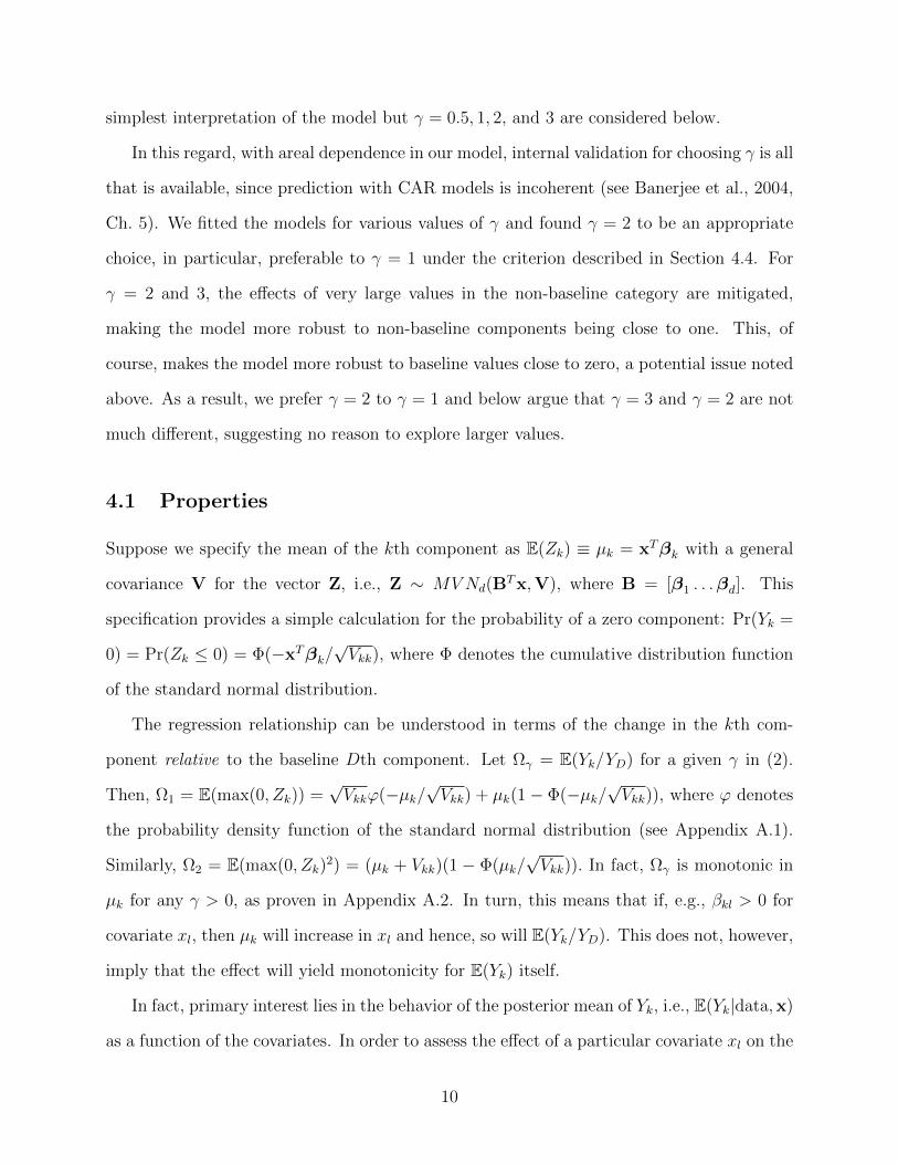
simplest interpretation of the model but γ = 0.5, 1, 2, and 3 are considered below.
In this regard, with areal dependence in our model, internal validation for choosing γ is all
that is available, since prediction with CAR models is incoherent (see Banerjee et al., 2004,
Ch. 5). We fitted the models for various values of γ and found γ = 2 to be an appropriate
choice, in particular, preferable to γ = 1 under the criterion described in Section 4.4. For
γ = 2 and 3, the effects of very large values in the non-baseline category are mitigated,
making the model more robust to non-baseline components being close to one. This, of
course, makes the model more robust to baseline values close to zero, a potential issue noted
above. As a result, we prefer γ = 2 to γ = 1 and below argue that γ = 3 and γ = 2 are not
much different, suggesting no reason to explore larger values.
4.1 Properties
Suppose we specify the mean of the kth component as E(Zk) ≡ µk = xTβk with a general
covariance V for the vector Z, i.e., Z ∼ MVNd(BTx,V), where B = [β1 . . .βd]. This
specification provides a simple calculation for the probability of a zero component: Pr(Yk =
0) = Pr(Zk ≤ 0) = Φ(−xTβk/√Vkk), where Φ denotes the cumulative distribution function
of the standard normal distribution.
The regression relationship can be understood in terms of the change in the kth com-
ponent relative to the baseline Dth component. Let Ωγ = E(Yk/YD) for a given γ in (2).
Then, Ω1 = E(max(0, Zk)) =√Vkkϕ(−µk/
√Vkk) + µk(1− Φ(−µk/
√Vkk)), where ϕ denotes
the probability density function of the standard normal distribution (see Appendix A.1).
Similarly, Ω2 = E(max(0, Zk)2) = (µk + Vkk)(1 − Φ(µk/
√Vkk)). In fact, Ωγ is monotonic in
µk for any γ > 0, as proven in Appendix A.2. In turn, this means that if, e.g., βkl > 0 for
covariate xl, then µk will increase in xl and hence, so will E(Yk/YD). This does not, however,
imply that the effect will yield monotonicity for E(Yk) itself.
In fact, primary interest lies in the behavior of the posterior mean of Yk, i.e., E(Yk|data,x)
as a function of the covariates. In order to assess the effect of a particular covariate xl on the
10

expected response of a particular component, Yk, we would like to track the movement of
the posterior mean over [0, 1] as xl is varied, holding the other covariates fixed (say, at their
mean levels). Unfortunately, E(Yk|data,x) = E(gk(B,V,x)|data,x) involves an untractable
function gk(B,V,x) = E(Yk|B,V,x). However, with MCMC model fitting, the conditional
distribution [Yk|data,x] can be sampled by composition using posterior samples of B and V
and making draws of Y from [Y|B,V,x]. These posterior samples will provide a Monte Carlo
integration for E(Yk|data,x) over a range of xl’s. The analyses in Section 6 supply such a
posterior summary across components and covariates for the LULC and forest fragmentation
datasets.
4.2 The hierarchical model and prior specifications
With cells indexed by i = 1, 2, ..., n, in the non-spatial model we have conditionally inde-
pendent Yi’s generated from latent Zi’s, with component k having mean E(Zik) = xTi βk.
To introduce spatial dependence, E(Zik) is revised to E(Zik) = xTi βk + φik. Here, φi =
(φi1, φi2, ..., φid)T is a vector of spatial random effects for cell i and φini=1 follow a d-
dimensional multivariate CAR model specified explicitly below. The regression coefficients
are fitted in the presence of the spatial random effects but the resulting interpretation with
regard to regression relationships is as in the non-spatial case. In our first example, Forest is
used as the baseline variable, which allows us to capture how changes in covariates affect the
proportions of the other components relative to the Forest category. We can also implement
the covariate analysis proposed above for E(Yk|data,x) in the spatial case, setting the spatial
effects to 0.
The Bayesian model is fully specified after including the prior distributions for the pa-
rameters, as shown below in (3). The notation j ∼ i means that cell j is a contiguous
neighbor of cell i and ni is the number of neighbors that cell i has. The number of covariates
is denoted by p and the number of grid cells is n. The full multi-level model is:
11
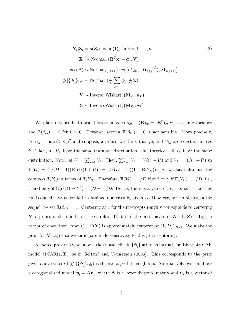
Yi|Zi = g(Zi) as in (1), for i = 1, . . . , n (3)
Ziind∼ Normald
(BTxi + φi,V
)vec(B) ∼ Normald(p+1)
(vec([µ1d×1 0d×p
]T ), λId(p+1)
)φi|φjj 6=i ∼ Normald
(1ni
∑j∼i
φj,1ni
Σ)
V ∼ Inverse Wishartd(MV ,mV
)Σ ∼ Inverse Wishartd
(MΣ,mΣ
)We place independent normal priors on each βkl ≡ (B)lk = (BT )kl with a large variance
and E(βkl) = 0 for l > 0. However, setting E(βk0) = 0 is not sensible. More precisely,
let Uk = max(0, Zk)2 and suppose, a priori, we think that µk and Vkk are constant across
k. Then, all Uk have the same marginal distribution, and therefore all Yk have the same
distribution. Now, let U =∑d
k=1 Uk. Then,∑d
k=1 Yk = U/(1 + U) and YD = 1/(1 + U) so
E(Yk) = (1/(D − 1))E(U/(1 + U)) = (1/(D − 1))(1 − E(YD)), i.e., we have obtained the
common E(Yk) in terms of E(YD). Therefore, E(Yk) = 1/D if and only if E(YD) = 1/D, i.e.,
if and only if E(U/(1 + U)) = (D − 1)/D. Hence, there is a value of µk = µ such that this
holds and this value could be obtained numerically, given D. However, for simplicity, in the
sequel, we set E(βk0) = 1. Centering at 1 for the intercepts roughly corresponds to centering
Y, a priori, in the middle of the simplex. That is, if the prior mean for Z is E(Z) = 1d×1, a
vector of ones, then, from (1), E(Y) is approximately centered at (1/D)1D×1. We make the
prior for V vague so we anticipate little sensitivity to this prior centering.
As noted previously, we model the spatial effects φi using an intrinsic multivariate CAR
model MCAR(1,Σ), as in Gelfand and Vounatsou (2003). This corresponds to the prior
given above where E(φi|φjj 6=i) is the average of its neighbors. Alternatively, we could use
a coregionalized model φi = Aui, where A is a lower diagonal matrix and ui is a vector of
12
independent univariate intrinsic CAR (1, σ2) models (Gelfand et al., 2004). Specification to
make these priors equivalent can be provided. The usual benefits of coregionalization include
univariate updates of each univariate CAR process. However, we do not gain that advantage
here because of the nonzero off-diagonals in the covariance matrix V. To identify the intrinsic
specification of the MCAR model, we assume that each dimension of the MCAR process sums
to zero, i.e.,∑n
i=1 φik = 0 for each k = 1, . . . , d. This is implemented computationally by
centering each dimension on the fly, as in Besag et al. (1995).
4.3 Model fitting
With the prior specification complete, posterior computation is done by Gibbs sampling.
The full conditional distributions are presented in Appendix B. The regression coefficients
B are updated simultaneously, using the fact that the prior and full conditional can be
written as a matrix Normal distribution. Assuming that X has been centered and scaled,
we set λ = 10 in the covariance for B, a weak specification since prior predictive simulations
show that effects for a scaled covariate will rarely be larger than 1. V and Σ are updated
from Inverse Wishart distributions, with scale matrices MV = MΣ = 2Id and degrees of
freedom mV = mΣ = d+ 3. This specification provides E(V) = E(Σ) = Id, which implies a
priori independence among the components.
The MCAR prior for the spatial effects provides local updating in the MCMC, i.e., the
vector φi, consisting of d random spatial effects, is updated as a unit. Though this is
straightforward, the need to update one location at a time still leads to a bottleneck with
regard to computational run time. However, due to the local structure of the MCAR model,
it is possible to usefully parallelize the updating process by dividing the region into blocks
and updating within the blocks in parallel, followed by updating the locations on the borders
of the blocks (Chakraborty et al., 2010). The number of blocks must be chosen to balance the
speed gains by adding more blocks with the speed costs due to increased overhead of more
blocks. For our analysis, with over 19,000 locations, the ability to update the spatial effects
13
in parallel blocks provides significant speed gains; we achieved good efficiency with four
blocks. Furthermore, the covariance matrix for each of these local updates is just a function
of the number of neighbors, which implies that there are only a few unique combinations to
be calculated each MCMC iteration.
We note that the negative, latent Zi’s can also be updated in parallel fashion due to the
conditional independence of the Zi’s. That is, a latent component of Zi, corresponding to a
zero Yi component, needs to be imputed through Gibbs sampling in order to enable sampling
of the model parameters and the spatial effects. When a large number of zero components
are observed, the need to sample the latent Zi’s can significantly decrease the efficiency of
the computation unless parallelization is introduced. Fortunately, the parallelization scheme
for the Zi’s is even simpler to implement than that for the φi’s.
4.4 Choosing γ
Choosing a value for γ is a model selection issue which we addressed by fitting the 2006
LULC data for several values of γ. Given that the predicted values contain point masses at
zero proportions, we used the continuous ranked probability score (CRPS) (Unger, 1985)
to provide comparison between observed values and the sampled posterior predictive values.
The CRPS is a proper scoring rule (Gneiting and Raftery, 2007) which compares the posterior
predictive CDF F to the empirical (degenerate) CDF for an observed value y using
CRPS(F, y) =
∫ ∞−∞
[F (x)− 1(x ≥ y)]2 dx, (4)
where 1(·) is the indicator function.
The CRPS is especially useful in our context because the comparison of distribution
functions seamlessly integrates the point masses at zero and values in the unit interval,
which will arise from predictions using our compositional data model. For an observed value
y = 0, the CRPS will prefer the point mass over any predictions in the unit interval and will
14
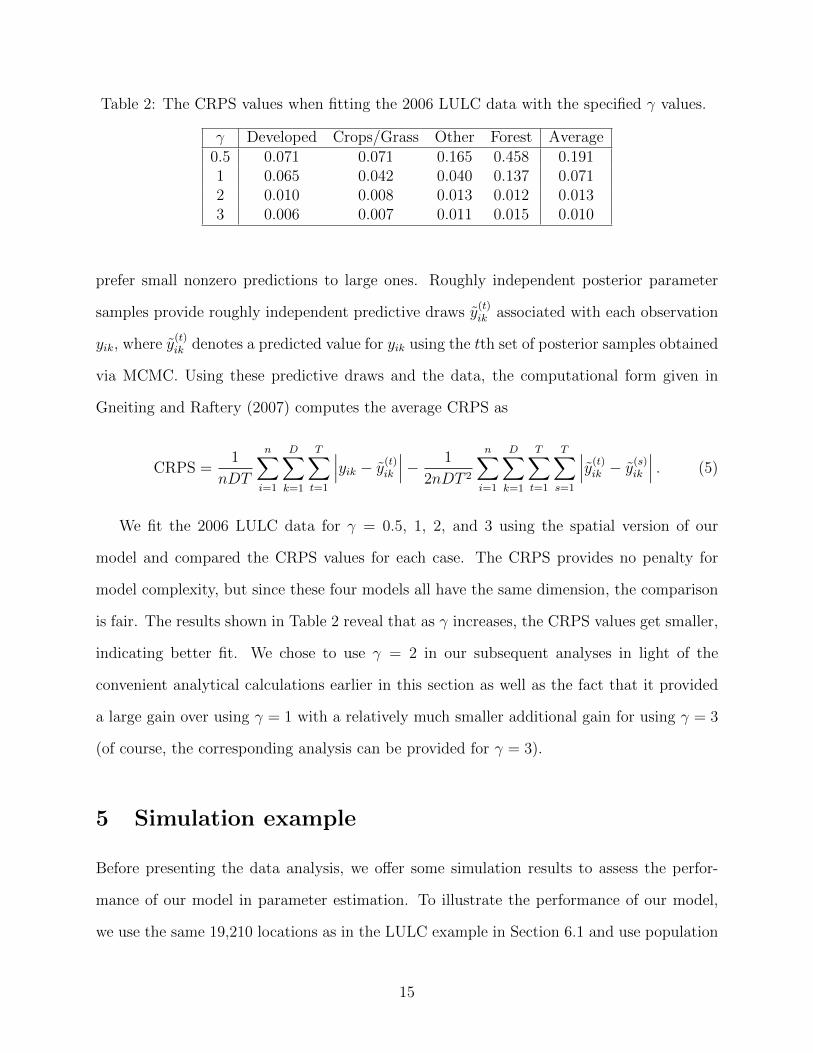
Table 2: The CRPS values when fitting the 2006 LULC data with the specified γ values.
γ Developed Crops/Grass Other Forest Average0.5 0.071 0.071 0.165 0.458 0.1911 0.065 0.042 0.040 0.137 0.0712 0.010 0.008 0.013 0.012 0.0133 0.006 0.007 0.011 0.015 0.010
prefer small nonzero predictions to large ones. Roughly independent posterior parameter
samples provide roughly independent predictive draws y(t)ik associated with each observation
yik, where y(t)ik denotes a predicted value for yik using the tth set of posterior samples obtained
via MCMC. Using these predictive draws and the data, the computational form given in
Gneiting and Raftery (2007) computes the average CRPS as
CRPS =1
nDT
n∑i=1
D∑k=1
T∑t=1
∣∣∣yik − y(t)ik
∣∣∣− 1
2nDT 2
n∑i=1
D∑k=1
T∑t=1
T∑s=1
∣∣∣y(t)ik − y
(s)ik
∣∣∣ . (5)
We fit the 2006 LULC data for γ = 0.5, 1, 2, and 3 using the spatial version of our
model and compared the CRPS values for each case. The CRPS provides no penalty for
model complexity, but since these four models all have the same dimension, the comparison
is fair. The results shown in Table 2 reveal that as γ increases, the CRPS values get smaller,
indicating better fit. We chose to use γ = 2 in our subsequent analyses in light of the
convenient analytical calculations earlier in this section as well as the fact that it provided
a large gain over using γ = 1 with a relatively much smaller additional gain for using γ = 3
(of course, the corresponding analysis can be provided for γ = 3).
5 Simulation example
Before presenting the data analysis, we offer some simulation results to assess the perfor-
mance of our model in parameter estimation. To illustrate the performance of our model,
we use the same 19,210 locations as in the LULC example in Section 6.1 and use population
15
as a covariate. We chose to have four components in the response (D = 4). The parameter
values considered are
BT =
0.15 0.15
0.3 −0.15
0.5 0
, V =
0.01 0 −0.005
0 0.02 0.005
−0.005 0.005 0.01
, and Σ =
0.2 0.02 −0.05
0.02 0.1 0.05
−0.05 0.05 0.1
.
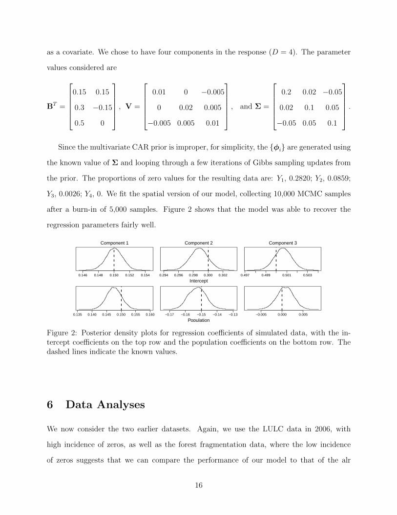
Since the multivariate CAR prior is improper, for simplicity, the φi are generated using
the known value of Σ and looping through a few iterations of Gibbs sampling updates from
the prior. The proportions of zero values for the resulting data are: Y1, 0.2820; Y2, 0.0859;
Y3, 0.0026; Y4, 0. We fit the spatial version of our model, collecting 10,000 MCMC samples
after a burn-in of 5,000 samples. Figure 2 shows that the model was able to recover the
regression parameters fairly well.
0.146 0.148 0.150 0.152 0.154
Component 1
0.294 0.296 0.298 0.300 0.302
Component 2
Intercept0.497 0.499 0.501 0.503
Component 3
0.135 0.140 0.145 0.150 0.155 0.160 −0.17 −0.16 −0.15 −0.14 −0.13
Population−0.005 0.000 0.005
Figure 2: Posterior density plots for regression coefficients of simulated data, with the in-tercept coefficients on the top row and the population coefficients on the bottom row. Thedashed lines indicate the known values.
6 Data Analyses
We now consider the two earlier datasets. Again, we use the LULC data in 2006, with
high incidence of zeros, as well as the forest fragmentation data, where the low incidence
of zeros suggests that we can compare the performance of our model to that of the alr
16
model. In both cases, we use the covariates described in Section 3 to explain changes in the
composition of the responses at each location. The models fitted in each analysis ran for
50,000 iterations after a 5,000 iteration burn-in and we retained every fifth sample, resulting
in 10,000 posterior samples. MCMC convergence was monitored using standard algorithms
provided by the coda package in R (Plummer et al., 2006).
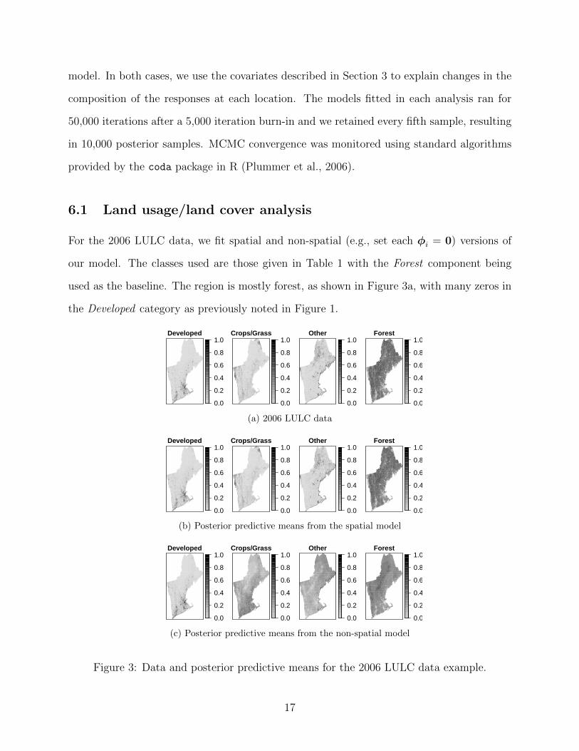
6.1 Land usage/land cover analysis
For the 2006 LULC data, we fit spatial and non-spatial (e.g., set each φi = 0) versions of
our model. The classes used are those given in Table 1 with the Forest component being
used as the baseline. The region is mostly forest, as shown in Figure 3a, with many zeros in
the Developed category as previously noted in Figure 1.
Developed
0.0
0.2
0.4
0.6
0.8
1.0Crops/Grass
0.0
0.2
0.4
0.6
0.8
1.0Other
0.0
0.2
0.4
0.6
0.8
1.0Forest
0.0
0.2
0.4
0.6
0.8
1.0
(a) 2006 LULC data
Developed
0.0
0.2
0.4
0.6
0.8
1.0Crops/Grass
0.0
0.2
0.4
0.6
0.8
1.0Other
0.0
0.2
0.4
0.6
0.8
1.0Forest
0.0
0.2
0.4
0.6
0.8
1.0
(b) Posterior predictive means from the spatial model
Developed
0.0
0.2
0.4
0.6
0.8
1.0Crops/Grass
0.0
0.2
0.4
0.6
0.8
1.0Other
0.0
0.2
0.4
0.6
0.8
1.0Forest
0.0
0.2
0.4
0.6
0.8
1.0
(c) Posterior predictive means from the non-spatial model
Figure 3: Data and posterior predictive means for the 2006 LULC data example.
17

Figure 3 shows the fit of the posterior predictive means to the LULC data for both the
spatial and non-spatial models. We note that the spatial model yields a very similar picture
when compared with the actual data, capturing the local variation in each of the components
while introducing a small amount of smoothing. The non-spatial version, however, only
seems to perform well for the Developed category, failing to capture much of the detail in the
remaining components. Though including additional covariates might help to ameliorate this
issue, the spatial random effects are evidently successful in capturing the local dependence
structure.
We then compared the models with and without spatial random effects using continuous
ranked probability scores as a rough guide for model comparison, though the issue with
model dimension is at hand here. The CRPS for each model is shown in Table 3, indicating
a very strong preference for the spatial version of the model. In fact, in terms of CRPS, the
spatial model was, on average, more than five times closer to the observed values than the
non-spatial version.
Table 3: Comparison of CRPS for non-spatial and spatial versions of our model on the 2006LULC data.
Model Developed Crops/Grass Other Forest AverageNon-spatial 0.023 0.042 0.095 0.119 0.070Spatial 0.010 0.008 0.014 0.020 0.013
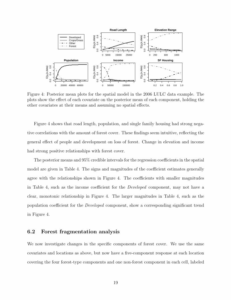
Illustration of the effects of the regression coefficients is given in Figure 4, where the
change in the posterior mean for each component can be seen as a function of the change in
the covariate level. These plots show E(Yk|data,x), the posterior mean for a component Yk
given the data and a covariate value xl, changing one covariate at a time while holding the
other covariates at their mean. We see how changing each covariate affects the posterior mean
for each component, taking into account the indirect effects of the regression coefficients, the
intercepts for each component, and the correlation structure in V. These plots assume no
spatial effect is present; adding a spatial effect will modify the local regression intercepts.
18
DevelopedCrops/GrassOtherForest
0 5000 15000 25000
0.0
0.4
0.8
Road Length
E(y
k|x,
data
)
0 200 600 1000
0.0
0.4
0.8
Elevation Range
E(y
k|x,
data
)
0 20000 40000 60000
0.0
0.4
0.8
Population
E(y
k|x,
data
)
0 50000 150000
0.0
0.4
0.8
Income
E(y
k|x,
data
)
0.2 0.4 0.6 0.8 1.0
0.0
0.4
0.8
SF Housing
E(y
k|x,
data
)
Figure 4: Posterior mean plots for the spatial model in the 2006 LULC data example. Theplots show the effect of each covariate on the posterior mean of each component, holding theother covariates at their means and assuming no spatial effects.
Figure 4 shows that road length, population, and single family housing had strong nega-
tive correlations with the amount of forest cover. These findings seem intuitive, reflecting the
general effect of people and development on loss of forest. Change in elevation and income
had strong positive relationships with forest cover.
The posterior means and 95% credible intervals for the regression coefficients in the spatial
model are given in Table 4. The signs and magnitudes of the coefficient estimates generally
agree with the relationships shown in Figure 4. The coefficients with smaller magnitudes
in Table 4, such as the income coefficient for the Developed component, may not have a
clear, monotonic relationship in Figure 4. The larger magnitudes in Table 4, such as the
population coefficient for the Developed component, show a corresponding significant trend
in Figure 4.
6.2 Forest fragmentation analysis
We now investigate changes in the specific components of forest cover. We use the same
covariates and locations as above, but now have a five-component response at each location
covering the four forest-type components and one non-forest component in each cell, labeled
19

Table 4: Posterior means and 95% credible intervals for the regression coefficients for thespatial model using the 2006 LULC data. The Forest category is used as the baseline.
Covariate Developed Crops/Grass OtherIntercept 0.277 (0.274, 0.280) 0.326 (0.325, 0.327) 0.513 (0.512, 0.515)Road Length 0.114 (0.109, 0.120) 0.047 (0.043, 0.050) -0.057 (-0.067, -0.047)Elevation Range -0.047 (-0.056, -0.038) -0.059 (-0.065, -0.054) -0.129 (-0.145, -0.113)Population 0.435 (0.427, 0.444) 0.087 (0.080, 0.093) -0.030 (-0.046, -0.013)Income -0.098 (-0.111, -0.084) -0.050 (-0.060, -0.041) -0.874 (-0.900, -0.844)SF Housing 0.026 (0.011, 0.041) 0.023 (0.013, 0.033) 0.245 (0.214, 0.275)
as the Other category. The Other category is used as the baseline here, since it has no zero
values.
Again, we fit a spatial and non-spatial version of our model, but we now compare the
results to the alternative of using the alr transformation on the data. For the alr, we assign
a small value, 0.01, where a zero occurs, and rescale the remaining non-zero components as
in the multiplicative strategy of Martın-Fernandez et al. (2003). This imputed dataset can
now be used to fit the alr model, though we use the original, non-imputed dataset for model
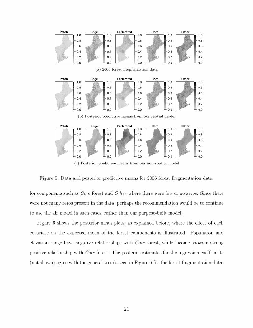
comparison via CRPS. Figure 5 shows the data and the posterior predictive means for the
2006 forest fragmentation data for the spatial and non-spatial versions of our model. Again,
the spatial version strongly outperforms the non-spatial version in terms of model fit.
Table 5: Comparison of CRPS for non-spatial and spatial versions of our point mass model(PM) and the alr model using the 2006 forest fragmentation data.
Model Spatial effects Patch Edge Perforated Core Other AveragePM Non-spatial 0.010 0.023 0.015 0.056 0.085 0.038PM Spatial 0.004 0.007 0.005 0.020 0.022 0.012alr Spatial 0.006 0.007 0.004 0.012 0.011 0.008
We use CRPS to compare the spatial and non-spatial models, also adding the CRPS for
the alr transformation with spatial effects. From Table 4, again, the non-spatial version of
our model had a much higher CRPS, roughly three times larger than the spatial version of
our model. We see, in Table 5, that our model seems to do a bit worse than the alr model
20
Patch
0.0
0.2
0.4
0.6
0.8
1.0Edge
0.0
0.2
0.4
0.6
0.8
1.0Perforated
0.0
0.2
0.4
0.6
0.8
1.0Core
0.0
0.2
0.4
0.6
0.8
1.0Other
0.0
0.2
0.4
0.6
0.8
1.0
(a) 2006 forest fragmentation data
Patch
0.0
0.2
0.4
0.6
0.8
1.0Edge
0.0
0.2
0.4
0.6
0.8
1.0Perforated
0.0
0.2
0.4
0.6
0.8
1.0Core
0.0
0.2
0.4
0.6
0.8
1.0Other
0.0
0.2
0.4
0.6
0.8
1.0
(b) Posterior predictive means from our spatial model
Patch
0.0
0.2
0.4
0.6
0.8
1.0Edge
0.0
0.2
0.4
0.6
0.8
1.0Perforated
0.0
0.2
0.4
0.6
0.8
1.0Core
0.0
0.2
0.4
0.6
0.8
1.0Other
0.0
0.2
0.4
0.6
0.8
1.0
(c) Posterior predictive means from our non-spatial model
Figure 5: Data and posterior predictive means for 2006 forest fragmentation data.
for components such as Core forest and Other where there were few or no zeros. Since there
were not many zeros present in the data, perhaps the recommendation would be to continue
to use the alr model in such cases, rather than our purpose-built model.
Figure 6 shows the posterior mean plots, as explained before, where the effect of each
covariate on the expected mean of the forest components is illustrated. Population and
elevation range have negative relationships with Core forest, while income shows a strong
positive relationship with Core forest. The posterior estimates for the regression coefficients
(not shown) agree with the general trends seen in Figure 6 for the forest fragmentation data.
21

PatchEdgePerforatedCoreOther
0 5000 15000 25000
0.0
0.4
0.8
Road Length
E(y
k|x,
data
)
0 200 600 1000
0.0
0.4
0.8
Elevation Range
E(y
k|x,
data
)
0 20000 40000 60000
0.0
0.4
0.8
Population
E(y
k|x,
data
)
0 50000 150000
0.0
0.4
0.8
Income
E(y
k|x,
data
)
0.2 0.4 0.6 0.8 1.0
0.0
0.4
0.8
SF Housing
E(y
k|x,
data
)
Figure 6: Posterior mean plots for the spatial version of our model on 2006 forest fragmen-tation data.
6.3 Sensitivity to grid cell resolution
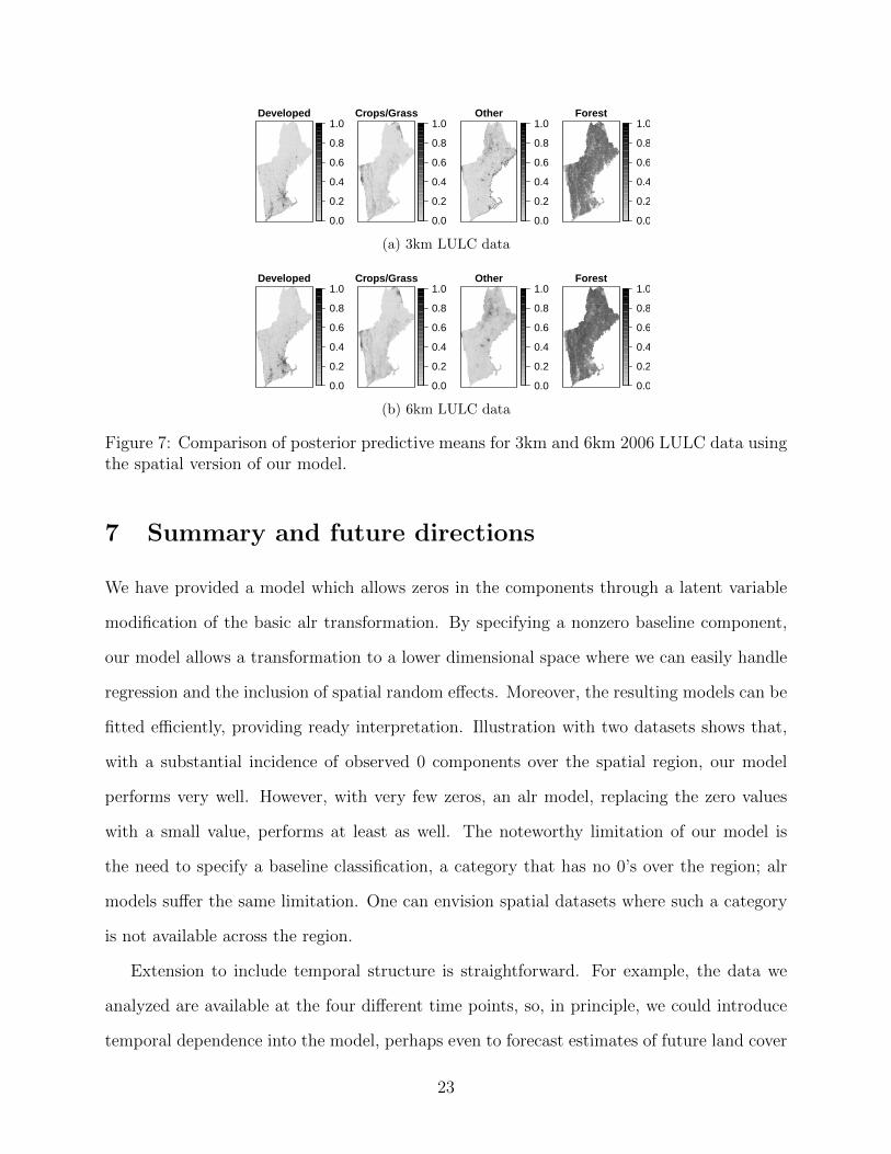
Finally, we compare the results at different resolutions. We present the posterior predictive
means using our spatial model with the 2006 LULC data at 3km and at 6km resolution. The
6km resolution dataset contains 4,614 observations, compared to the 19,210 observations
in the 3km dataset, and the developed class still has a large incidence of observed zero
proportions.
The averaging to achieve the lower resolution implies less local detail in the 6km dataset.
In Figure 7, we see that very similar predicted values are obtained for both the 3km and 6km
datasets. However, for the latter, the resultant smoothing succeeds in losing many of the
high values in the Other category along the eastern coast. The fitted regression coefficients
tell the same story at both scales (not shown). The variance components, i.e., the entries in
V, tend to be a bit larger at the 3km scale, reflecting the increased detail, hence increased
component variability, at the higher resolution (again, not shown). In summary, the 3km
and 6km grid cells are artificial partitions of a continuous landscape but we find consistent
inference results between the resolutions.
22
Developed
0.0
0.2
0.4
0.6
0.8
1.0Crops/Grass
0.0
0.2
0.4
0.6
0.8
1.0Other
0.0
0.2
0.4
0.6
0.8
1.0Forest
0.0
0.2
0.4
0.6
0.8
1.0
(a) 3km LULC data
Developed
0.0
0.2
0.4
0.6
0.8
1.0Crops/Grass
0.0
0.2
0.4
0.6
0.8
1.0Other
0.0
0.2
0.4
0.6
0.8
1.0Forest
0.0
0.2
0.4
0.6
0.8
1.0
(b) 6km LULC data
Figure 7: Comparison of posterior predictive means for 3km and 6km 2006 LULC data usingthe spatial version of our model.
7 Summary and future directions
We have provided a model which allows zeros in the components through a latent variable
modification of the basic alr transformation. By specifying a nonzero baseline component,
our model allows a transformation to a lower dimensional space where we can easily handle
regression and the inclusion of spatial random effects. Moreover, the resulting models can be
fitted efficiently, providing ready interpretation. Illustration with two datasets shows that,
with a substantial incidence of observed 0 components over the spatial region, our model
performs very well. However, with very few zeros, an alr model, replacing the zero values
with a small value, performs at least as well. The noteworthy limitation of our model is
the need to specify a baseline classification, a category that has no 0’s over the region; alr
models suffer the same limitation. One can envision spatial datasets where such a category
is not available across the region.
Extension to include temporal structure is straightforward. For example, the data we
analyzed are available at the four different time points, so, in principle, we could introduce
temporal dependence into the model, perhaps even to forecast estimates of future land cover
23

patterns. However, as there was little change evident in the data, we have not investigated
this. Another path to explore would be joint modeling of LULC and forest fragmentation in
order to see if joint analysis benefits our explanatory story.
One issue we have not addressed here is that of potential spatial confounding between
the fixed effects in the regression and random effects in the multivariate CAR model. The
results presented here exhibited some spatial confounding when comparing the spatial and
non-spatial models. The results were similar for both versions, though the regression effects
in the spatial model were generally stronger than in the non-spatial model, making the
effects in Figure 4 more dramatic than those in the non-spatial model. In one case, for the
population effect on the Other component in the LULC analysis, the regression coefficient
switched signs when removing the spatial effects.
Hence, future work to address spatial confounding might prove beneficial. The papers
of Reich et al. (2006) and Hughes and Haran (2013) provide methods for alleviating this
problem, though these approaches would be more challenging for multivariate spatial random
effects.
Appendices
A Calculations using Ωγ
Without loss of generality, we’ll assume Zk has mean µ and variance v and let φ and Φ denote
the probability density and distribution functions of the standard normal distribution.
24

A.1 Value of Ω1
We can calculate, letting γ = 1, the value of Ω1 as
Ω1 = Emax(0, Zk) =
∫ ∞−∞
max(0, z)pZk(z)dz =
∫ ∞0
z pZk(z)dz
=
∫ ∞0
z1√2πv
exp
−(z − µ)2
2v
dz
=
∫ ∞0
(z − µ)1√2πv
exp
−(z − µ)2
2v
dz +
∫ ∞0
µ1√2πv
exp
−(z − µ)2
2v
dz
=
(−√v√
2πexp
−(z − µ)2
2v
) ∣∣∣∣∞0
+ µ(1− Φ(−µ/√v))
=√vφ(−µ/
√v) + µ(1− Φ(−µ/
√v)).
The proof for Ω2 is similar.
A.2 Proof of monotonicity of Ωγ
Start by modifying the notation to write Ωγ(µ, v) as an explicit function of µ and v. Without
loss of generality, consider increasing µ to µ+ δ for some δ > 0. We see that
Ωγ(µ+ δ, v) =
∫ ∞0
z1√2πv
exp−(z − µ− δ)2/2v
dz
=
∫ ∞−δ
(y + δ)1√2πv
exp−(y − µ)2/2v
dy
=
∫ 0
−δ(y + δ)
1√2πv
exp−(y − µ)2/2v
dy︸ ︷︷ ︸
> 0
+
∫ ∞0
(y + δ)1√2πv
exp−(y − µ)2/2v
dy︸ ︷︷ ︸
> Ωγ(µ, v) because (y + δ) > y
> Ωγ(µ, v).
Hence Ωγ is a monotonically increasing function in µk for arbitrary γ.
25

B Full conditionals for spatial regression model
[vec(B)|−] ∼ Normal(Ω(V−1 ⊗XTX)(XTX)−1
∑i
xTi (Zi − φi) , Ω)
where Ω = (λ−1Id×p + V−1 ⊗XTX)−1
[V|−] ∼ Inverse Wishart(mV + n, MV +
∑i
(Zi −BTxi − φi)(Zi −BTxi − φi)T)
[φi|−] ∼ Normald((V−1 + niΣ
−1)−1(V−1(Zi −BTxi) + Σ−1
(∑i∼j
φj
)), (V−1 + niΣ
−1)−1)
[Σ|−] ∼ Inverse Wishart(mΣ + n, MΣ +
∑i
∑j
(DW −W)ijφiφTj
)where DW is a diagonal matrix with elements (DW )ii = ni
and W is the spatial adjacency matrix with Wij = 1 if i ∼ j and 0 otherwise
Sample code can be found at http://stat.duke.edu/∼tjl13/research.html.
References
Aitchison, J. (1986), The Statistical Analysis of Compositional Data, Chapman and Hall,
New York.
Aitchison, J. and Egozcue, J. J. (2005), “Compositional Data Analysis: Where Are We and
Where Should We Be Heading?” Mathematical Geology, 37, 829–850.
Banerjee, S., Carlin, B. P., and Gelfand, A. E. (2004), Hierarchical modeling and analysis
for spatial data, Boca Raton, FL: Chapman and Hall/CRC Press.
Besag, J. (1974), “Spatial interaction and the statistical analysis of lattice systems,” Journal
of the Royal Statistical Society: Series B (Statistical Methodology), 36, 192–236.
Besag, J., Green, P., Higdon, D., and Mengersen, K. (1995), “Bayesian computation and
stochastic systems,” Statistical Science, 10, 3–66.
26
Billheimer, D., Cardoso, T., Freeman, E., Guttorp, P., Ko, H.-W., and Silkey, M. (1997),
“Natural variability of benthic species composition in the Delaware Bay,” Environmental
and Ecological Statistics, 4, 95–115.
Butler, A. and Glasbey, C. (2009), “Corrigendum: A latent Gaussian model for compositional
data with zeros,” Journal of the Royal Statistical Society: Series C (Applied Statistics),
58, 141–141.
Chakraborty, A., Gelfand, A., Wilson, A. M., Latimer, A. M., and Silander, J. A. (2010),
“Modeling large scale species abundance with latent spatial processes,” The Annals of
Applied Statistics, 4, 1403–1429.
Egozcue, J. J., Pawlowsky-Glahn, V., Mateu-Figueras, G., and Barcelo-Vidal, C. (2003),
“Isometric Logratio Transformations for Compositional Data Analysis,” Mathematical Ge-
ology, 35, 279–300.
Fry, J., Fry, T., and McLaren, K. (2000), “Compositional data analysis and zeros in micro
data,” Applied Economics, 32, 953–959.
Fry, J. A., Coan, M. J., Homer, C. G., Meyer, D. K., and Wickham, J. (2009), “Completion
of the National Land Cover Database (NLCD) 19922001 Land Cover Change Retrofit
Product,” U.S. Geological Survey Open-File Report 20081379, 18 p.
Gelfand, A. E., Schmidt, A. M., Banerjee, S., and Sirmans, C. F. (2004), “Nonstationary
multivariate process modelling through spatially varying coregionalization (with discus-
sion),” Test, 13, 1–50.
Gelfand, A. E. and Vounatsou, P. (2003), “Proper multivariate conditional autoregressive
models for spatial data analysis.” Biostatistics (Oxford, England), 4, 11–25.
Gneiting, T. and Raftery, A. E. (2007), “Strictly Proper Scoring Rules, Prediction, and
Estimation,” Journal of the American Statistical Association, 102, 359–378.
27
Haslett, J., Whiley, M., Bhattacharya, S., Salter-Townshend, M., Wilson, S. P., Allen, J.
R. M., Huntley, B., and Mitchell, F. J. G. (2006), “Bayesian palaeoclimate reconstruction,”
Journal of the Royal Statistical Society: Series A (Statistics in Society), 169, 395–438.
Hughes, J. and Haran, M. (2013), “Dimension reduction and alleviation of confounding for
spatial generalized linear mixed models,” Journal of the Royal Statistical Society: Series
B (Statistical Methodology), 75, 139–159.
Kent, J. T. (1982), “The Fisher-Bingham distribution on the sphere,” Journal of the Royal
Statistical Society: Series B (Statistical Methodology), 44, 71–80.
Mardia, K. V. (1988), “Multi-dimensional Multivariate Gaussian Markov Random Fields
with Application to Image Processing,” Journal of Multivariate Analysis, 284, 265–284.
Martın-Fernandez, J. A., Barcelo-Vidal, C., and Pawlowsky-Glahn, V. (2003), “Dealing with
zeros and missing values in compositional data sets using nonparametric imputation,”
Mathematical Geology, 35, 253–278.
Minnesota Population Center (2004), “National Historical Geographic Information System:
Pre-release Version 0.1,” University of Minnesota, Minneapolis, MN, available at: http:
//www.nhgis.org/.
National Oceanic and Atmospheric Administration (2006), “Coastal Change Analysis Pro-
gram Land Cover,” available at: http://www.csc.noaa.gov/crs/lca/northeast.html.
Parent, J. and Hurd, J. (2010), “Landscape Fragmentation Tool (LFT v2.0).” Center for
Land use Education and Research. Available at: http://clear.uconn.edu/tools/lft/
lft2/index.htm.
Plummer, M., Best, N., Cowles, K., and Vines, K. (2006), “CODA: Convergence Diagnosis
and Output Analysis for MCMC,” R News, 6, 7–11.
28
R Core Team (2012), R: A Language and Environment for Statistical Computing, R Foun-
dation for Statistical Computing, Vienna, Austria, ISBN 3-900051-07-0.
Reich, B. J., Hodges, J. S., and Zadnik, V. (2006), “Effects of Residual Smoothing on the
Posterior of the Fixed Effects in Disease-Mapping Models,” Biometrics, 62, 1197–1206.
Salter-Townshend, M. and Haslett, J. (2006), “Modelling zero inflation of compositional
data,” in Proceedings of the 21st International Workshop on Statistical Modelling, pp.
448–456.
Scealy, J. L. and Welsh, A. H. (2011), “Regression for compositional data by using distri-
butions defined on the hypersphere,” Journal of the Royal Statistical Society: Series B
(Statistical Methodology), 73, 351–375.
Stephens, M. A. (1982), “Use of the von Mises distribution to analyse continuous propor-
tions,” Biometrika, 69, 197–203.
Stewart, C. and Field, C. (2010), “Managing the essential zeros in quantitative fatty acid
signature analysis,” Journal of Agricultural, Biological, and Environmental Statistics, 16,
45–69.
Tjelmeland, H. and Lund, K. V. (2003), “Bayesian modelling of spatial compositional data,”
Journal of Applied Statistics, 30, 87–100.
Tsagris, M. T., Preston, S., and Wood, A. T. (2011), “A data-based power transformation
for compositional data,” in Proceedings of CoDaWork’11: 4th international workshop on
Compositional Data Analysis, eds. Egozcue, J., Tolosana-Delgado, R., and Ortego, M.
Unger, D. A. (1985), “A Method to Estimate the Continuous Ranked Probability Score,” in
Preprints of the Ninth Conference on Probability and Statistics in Atmospheric Sciences,
Virginia Beach, Virginia, American Meteorological Society, Boston, pp. 206–213.
29
U.S. Census Bureau (2008), “TIGER/Line Shapefiles [machine-readable data files],” avail-
able at: http://www.census.gov/geo/maps-data/data/tiger.html.
U.S. Geological Survey (1999), “National Elevation Dataset,” available at: http://
nationalmap.gov/viewer.html.
van den Boogaart, K. G. and Tolosana-Delgado, R. (2008), “compositions: A unified R
package to analyze compositional data,” Computers and Geosciences, 34, 320–338.
30
Related Documents