KERNEL REGRESSION ESTIMATION FOR SPATIAL ...

HAL Id: hal-00605923https://hal.archives-ouvertes.fr/hal-00605923

Preprint submitted on 4 Jul 2011

HAL is a multi-disciplinary open accessarchive for the deposit and dissemination of sci-entific research documents, whether they are pub-lished or not. The documents may come fromteaching and research institutions in France orabroad, or from public or private research centers.

L’archive ouverte pluridisciplinaire HAL, estdestinée au dépôt et à la diffusion de documentsscientifiques de niveau recherche, publiés ou non,émanant des établissements d’enseignement et derecherche français ou étrangers, des laboratoirespublics ou privés.

KERNEL REGRESSION ESTIMATION FORSPATIAL FUNCTIONAL RANDOM VARIABLES

Sophie Dabo-Niang, Mustapha Rachdi, Anne-Françoise yao

To cite this version:Sophie Dabo-Niang, Mustapha Rachdi, Anne-Françoise yao. KERNEL REGRESSION ESTIMATIONFOR SPATIAL FUNCTIONAL RANDOM VARIABLES. 2010. hal-00605923

Kernel regression estimation for spatial functional random

variables

Sophie Dabo-Niang ♯, Mustapha Rachdi ∓ and Anne-Françoise Yao §

Corresponding author : ♯ University Charles De Gaulle, Lille 3, Laboratoire EQUIPPE, maison de la

recherche, domaine du pont de bois, BP 60149, 59653 Villeneuve d’ascq cedex, France.

[email protected]

§ University Aix-Marseille 2, Laboratoire LMGEM, Campus de Luminy, case 901, 13288 Marseille

cedex 09, France. [email protected]

∓ University Grenoble 2, UFR SHS, BP. 47 38040 Grenoble Cedex 09 France,

[email protected]

Abstract

Given a spatial random process(Xi, Yi) ∈ E × R, i ∈ Z

N, we investigate a nonpara-

metric estimate of the conditional expectation of the real random variable Yi given the

functional random field Xi valued in a semi-metric space E . The weak and strong consis-

tencies of the estimate are shown and almost sure rates of convergence are given. Special

attention is paid to apply the regression estimate introduced to spatial prediction prob-

lems.

Key Words: Regression estimation; Random fields; Functional variables; Infinite dimen-

sional space; Small balls probabilities;.

1. Introduction

Nowadays, the progress of informatics tools permits the recuperation of increasingly

bulky data. These large data sets are available essentially by real time monitoring and

computers can manage such databases. The object of statistical study can then be curves

(consecutive discrete recordings are aggregated and viewed as sampled values of a random

curve) not numbers or vectors. Functional data analysis (see Bosq [4], Ferraty and Vieu

[18], Ramsay and Silverman [30]) can help to analyze such high-dimensional data sets.

The statistical problems involved in modeling functional random variables offer increasing

interests in recent literature. For prediction problems, functional data analysis techniques

outdo the other approaches because they take advantage of past information. See for

example Bosq [4], Besse et al. [2], Cardot and Johannes [8], Fernandez de Castro et al. [17],

Ferraty and Vieu [18], Dabo-Niang and Ferraty [11], Dabo-Niang and Rhomari [12], Ferré

Preprint submitted to Elsevier July 4, 2011

and Yao [19], Rachdi and Vieu [29] for some regression and forecasts results obtained by

several functional models (linear, nonlinear, neural networks and semi-parametric models)

for non spatial variables. It is proved in some of these papers that the best predictions

were generally obtained by the functional methods (either autoregressive or functional

kernel).

To the best of our knowledge, although potential applications of regression estimation

(or prediction) to functional spatial data are without number, only the papers of Dabo-

Niang and Yao [14], Delicado et al. [15] and Nerini et al. [28], have paid attention to study

regression or prediction for functional random fields.

The last two works deal with spatial kriging (linear predictor) methods for spatial

functional data. Dabo-Niang and Yao [14] introduced a nonparametric predictor for

functional random fields, for which the behavior has not been investigated. We want to

go further and extend functional data nonparametric analysis techniques to the spatial

domain. We suggest a nonparametric regression estimation approach which is to aggregate

over space.That is, we are mainly concerned with kernel regression methods for functional

random fields (spatial curves). Note that Lakasaci and Fouzia [23] considered the case

of conditional quantile estimation where the regressor take values in a semi-metric space

and showed the strong and weak consistency of the conditional quantile.

Spatial regression estimation is an interesting and crucial problem in statistical infer-

ence for a number of applications (as in a variety of fields, including soil science, geology,

oceanography, econometrics, epidemiology, environmental science, forestry,...), where the

influence of a vector of covariates on some response variable is to be studied in a context

of spatial dependence.

The literature on parametric spatial modeling is relatively abundant and we refer to Chilès

and P. [9], Guyon [20], Anselin and Florax [1], Cressie [10] or Ripley [32] for a list of ref-

erences. However, the nonparametric treatment of functional or multivariate spatial data

is limited. Actually, if some references on spatial nonparametric regression estimation in

the multidimensional setting (key refererences are: Lu and Chen [25, 26], Hallin et al.

[22], Hallin and Yu [21], Carbon et al. [5], Dabo-Niang and Yao [14], Li and Tran [24],...)

already exist, no work have been devoted to nonparametric regression for functionnal

spatial data. The aim of this paper is to study the behavior of the functional spatial

counterpart of the Nadaraya-Watson Nadaraya [27], Watson [34]’s estimator.

The paper is organized as follows. In Section 2, we provide the notations, assump-

tions and introduce a kernel estimate of the conditional mean. Section 3 is devoted to

convergence in probability and strong convergence of the kernel estimate. To check the

performance of our estimator, simulations results will be given in Section 4. Conclusion

is given on Section 5 and Proofs and technical lemmas are given in the last section.

2

2. General setting

Let ZN (N ≥ 1), be the integer lattice points in the N−dimensional Euclidean space.

A point in bold i = (i1, ..., iN) ∈ ZN will be referred as a site. In fact, spatial data can

be seen as realizations of a measurable strictly stationary spatial process Zi, defined on

a probability space (Ω, A,P). In this paper we deal with process of the feature: Zi =

(Xi, Yi), i ∈ ZN such that: the Z ′

is have the same distribution as a variable Z = (X, Y ),

where Y is a real-valued and integrable variable and X valued in a separable semi-metric

space (E , d(., .)) (of eventually infinite dimension).

In the following, we will denote by µ the probability distribution of X and ∀ i, j by

νi,j the joint probability distribution of (Xi, Xj), ‖.‖ will denote any norm over ZN , C an

arbitrary constant and B(x, ρ) the opened ball of center x and radius ρ. We will write

n → +∞ if mink=1,...,N nk → +∞ and we set n = n1 × ... × nN and NN , will denotes

subspace of ZN of vectors with non-negative components.

For a seek of simplicity, we will suppose that the variable Y is bounded. Instead of

this condition one can assume (as in Tran [33], Dabo-Niang and Yao [14] and Ferraty and

Vieu [18]) that one of the following assumptions holds:

• For all i 6= j, E [YiYj|(Xi, Xj)] ≤ C for some constant C > 0.

• For all m ≥ 2, E [Y m|X = x] ≤ gm(x) < ∞, where gm is a continuous function at

x ∈ E .

The proofs given here remain valid in one of these above cases.

2.1. The spatial kernel regression estimator for functional data

We aim to estimate the regression function r(x) = E (Y |X = x) of Y given X. To

do this, we propose the kernel estimate of the function r based on observations of the

process (Zi) in some region In and without the lost of generality, we suppose that In is

a rectangular region In :=i ∈N

N : 1 ≤ ik ≤ nk, k = 1, ..., N

:

rn(x) =

∑i∈In

YiWi,x if∑

i∈InWi,x 6= 0;

1bn

∑i∈In

Yi else.

where

Wi,x =K (d(Xi, x)h

−1n )∑

j∈InK (d(Xj, x)h−1

n ).

This estimate can also be written as follows:

3

rn(x) =

ϕn(x)/fn(x) if∑

i∈InWi,x 6= 0;

1bn

∑i∈In

Yi else.

with

ϕn(x) =1

nE (K (d(X, x)h−1n ))

∑

i∈In

YiK(d(Xi, x)h

−1n

), x ∈ E ,

fn (x) =1

nE (K (d(X, x)h−1n ))

∑

i∈In

K(d(Xi, x)h

−1n

), x ∈ E ,

where limn→+∞ hn = 0 (+) , the kernel K is a function from R+ to R

+.

That is an extension of the well known of Nadaraya [27], Watson [34]’s estimate in-

troduced for i.i.d observations.

Since we are dealing with spatial data, as any spatial model, ours must take into

account the dependance between observations. Let us now consider some measures of

dependence.

2.2. Spatial dependence measures

As it often occurs in spatial dependent data analysis, one needs to defined the type of

dependence. We consider here the following two dependence measures:

2.2.1. Local dependence condition

We assume also that for all i, j ∈ NN the joint probability distribution νi,j of Xi and

Xj satisfies

∃ǫ1 ∈ (0, 1], νi,j (B(x, hn) ×B(x, hn)) = (pxhn

)1+ǫ1 , (2.1)

where pxhn

= P (X ∈ B(x, hn)) = µ(B(x, hn)). We recall that νi,j is the joint distribution

of (Xi, Xj).

Remark 1. Note that this condition leads to νi,j (B(x, hn) ×B(x, hn)) −(px

hn

)2=

(pxhn

)2((px

hn)ǫ1−1 − 1

)≥ 0 so∣∣∣νi,j (B(x, hn) ×B(x, hn)) −

(px

hn

)2∣∣∣ = (pxhn

)2((px

hn)ǫ1−1 − 1

)≤ (px

hn)1+ǫ1 ≤ 1. Then, it

can be link with the classical local dependence condition met in the literature when Xand (Xi, Xj) admitted respectively the densities f and fi,j:

|fi,j (x, y) − f (x) f (y)| ≤ C,

for some constant C > 0 and for all x, y ∈ E and i, j ∈ NN , i 6= j.

Actually, this condition can be replace by the more general version (which is notnecessary here):

∃ǫ1 ∈ (0, 1], P ((Xi, Xj) ∈ B(x, hn) ×B(y, hn)) = (pxhnpy

hn)

1+ǫ12 ;

4

then,∣∣νi,j (B(x, hn) ×B(y, hn)) − px

hnpy

hn

∣∣ = (pxhnpy

hn)((px

hnpy

hn)

ǫ1−12 − 1

)≤ (px

hnpy

hn)

1+ǫ12 ≤

1.

Such local dependency condition is necessary to reach the same rate of convergence as

in the i.i.d. case.

2.2.2. Mixing conditions

Another complementary dependency condition concerned the mixing condition which

measures the dependency by means of α-mixing. We assume that(Zi, i ∈ Z

N)

satisfies

the following mixing condition: there exists a function ϕ (t) ↓ 0 as t → ∞, such that for

E, E′

subsets of ZN with finite cardinals,

α(B (E) , B

(E

′

))= sup

B∈B(E), C∈B(E′)|P (B ∩ C) − P (B)P (C)|

≤ χ(Card (E) ,Card

(E

′

))ψ(dist

(E,E

′

)), (2.2)

where B (E)(resp. B(E

′)) denotes the Borel σ-field generated by (Zi, i ∈ E) (resp.(

Zi, i ∈ E′)), Card(E) (resp. Card

(E

′)) the cardinality of E (resp. E

′

), dist(E, E

′)

the Euclidean distance between E and E′

and χ : N2 → R

+ is a nondecreasing symmet-

ric positive function in each variable. Throughout the paper, it will be assumed that χ

satisfies either

χ (n,m) ≤ Cmin (n,m) , ∀n,m ∈ N (2.3)

or

χ (n,m) ≤ C (n+m+ 1)eβ , ∀n,m ∈ N (2.4)

for some β ≥ 1 and some C > 0. If χ ≡ 1, then Zi is called strongly mixing. Many

stochastic processes, among them various useful time series models satisfy strong mixing

properties, which are relatively easy to check . Conditions (2.3)-(2.4) are weaker than

strong mixing condition and have been used for finite dimensional variables in (for exam-

ple) Tran [33], Carbon et al. [6, 7] and Biau and Cadre [3]. We refer to Doukhan [16] and

Rio [31] for discussion on mixing and examples.

Concerning the function ψ(.), we will only study the case where ψ(i) tends to zero at

a polynomial rate, ie.

ψ(i) ≤ Ci−θ, for some θ > 0. (2.5)

In the following, we denote by:

θ1 =−θ +N

N(1 + 2β) − θ, θ2 =

−θ + 2N

2N(β + 1) − θ,

5

θ3 =−θ +N

N(1 + 2β + 2β) − θ.

θ∗1 =2N − θ

4N − θ, θ∗2 =

−θ +N

N(2β + 3) − θ,

θ∗3 =−θ + 2N

−θ + 2N(β + 2), θ∗4 =

−θ +N

N(3 + 2β + 2β) − θ.

Remark 2. The results obtained below can be extend to the case where ψ(i) tends to zeroat an exponential rate: i.e ψ(i) = C exp(−si) for some s > 0.

• Each of the two dependence measures have the following specificity: if the first onecontrol the local dependence, the second one control the dependence of sites whichare far from each other.

• Clearly, one has, for a fixed hn (note that the same argument can be easily gener-alized to the case where one deals with two different bandwidths) :

α(‖i − j‖) ≥ ‖gi,j‖∞

withgi,j(x, y) = νi,j (B(x, hn) ×B(y, hn)) − px

hnpy

hn.

2.3. Assumptions on the kernel

We assume that the kernel K : R → R+ is of integral 1 and is such that:

HK1 : there exist two constants 0 < C1 < C2 <∞:

C1I[0,1] ≤ K ≤ C2I[0,1].

where I[0,1] is the indicator function in [0, 1].

or

The support of K is [0, 1], the derivative K ′ of K exists and satisfies

−∞ < C1 ≤ K ′ ≤ C2 < 0 and −∃C > 0,∃ε0 > 0,∀ε < ε0,

ˆ ε

0

µ(B(x, z)) dz > Cεµ(B(x, ε)).

In some cases, we will assume that:

HK2 : K is a Lipschitz function.

6

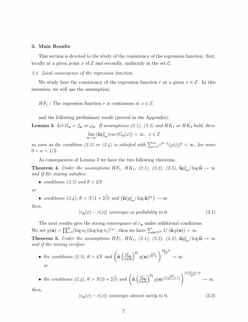
3. Main Results

This section is devoted to the study of the consistency of the regression function: first,

locally at a given point x of E and secondly, uniformly in the set C.

3.1. Local convergence of the regression function

We study here the consistency of the regression function r at a given x ∈ E . In this

intention, we will use the assumption:

HF1 - The regression function r is continuous at x ∈ E ,

and the following preliminary result (proved in the Appendix):

Lemma 3. Let Gn = fn or ϕn. If assumptions (2.1), (2.2) and HK1 or HK2 hold, then:

limn→∞

(npxhn

)var(Gn(x)) <∞, x ∈ E

as soon as the condition (2.3) or (2.4) is satisfied with∑∞

i=1 iN−1(ϕ(i))a < ∞, for some

0 < a < 1/2.

As consequences of Lemma 3 we have the two following theorems.

Theorem 4. Under the assumptions HF1, HK1, (2.1), (2.2), (2.5), npxhn/ log n → ∞

and if the mixing satisfies:

• conditions (2.3) and θ > 2N

or

• conditions (2.4), θ > N(1 + 2β) and(n(px

hn/ log n)θ1

)→ ∞

then,|rn(x) − r(x)| converges in probability to 0. (3.1)

The next results give the strong convergence of rn under additional conditions.

We set g(n) =∏N

i=1(log ni)(log log ni)1+ǫ, then we have

∑n∈NN 1/ (n g(n)) <∞.

Theorem 5. Under the assumptions HF1, HK1, (2.1), (2.2), (2.5), npxhn/ log n → ∞

and if the mixing verifies:

• the conditions (2.3), θ > 4N and

(n(

pxhn

log bn

)θ∗1g(n)

2N4N−θ

) 4N−θ2N

→ ∞

or

• the conditions (2.4), θ > N(3 + 2β) and

(n(

pxhn

log bn

)θ∗2g(n)

2N

N(2eβ+3)−θ

)N(2eβ+3)−θ

2N

→ ∞

then,|rn(x) − r(x)| converges almost surely to 0. (3.2)

7

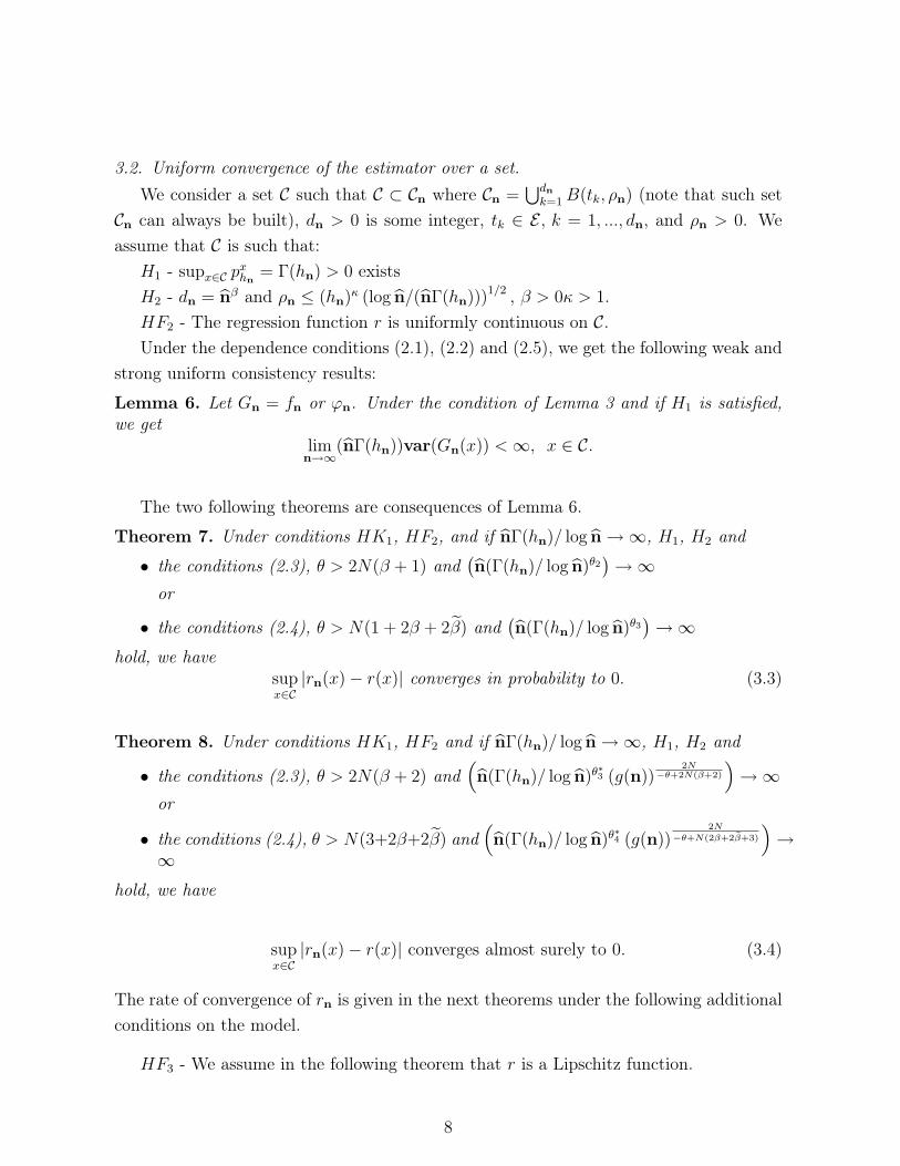
3.2. Uniform convergence of the estimator over a set.

We consider a set C such that C ⊂ Cn where Cn =⋃dn

k=1B(tk, ρn) (note that such set

Cn can always be built), dn > 0 is some integer, tk ∈ E , k = 1, ..., dn, and ρn > 0. We

assume that C is such that:

H1 - supx∈C pxhn

= Γ(hn) > 0 exists

H2 - dn = nβ and ρn ≤ (hn)κ (log n/(nΓ(hn)))1/2 , β > 0κ > 1.

HF2 - The regression function r is uniformly continuous on C.

Under the dependence conditions (2.1), (2.2) and (2.5), we get the following weak and

strong uniform consistency results:

Lemma 6. Let Gn = fn or ϕn. Under the condition of Lemma 3 and if H1 is satisfied,we get

limn→∞

(nΓ(hn))var(Gn(x)) <∞, x ∈ C.

The two following theorems are consequences of Lemma 6.

Theorem 7. Under conditions HK1, HF2, and if nΓ(hn)/ log n → ∞, H1, H2 and

• the conditions (2.3), θ > 2N(β + 1) and(n(Γ(hn)/ log n)θ2

)→ ∞

or

• the conditions (2.4), θ > N(1 + 2β + 2β) and(n(Γ(hn)/ log n)θ3

)→ ∞

hold, we havesupx∈C

|rn(x) − r(x)| converges in probability to 0. (3.3)

Theorem 8. Under conditions HK1, HF2 and if nΓ(hn)/ log n → ∞, H1, H2 and

• the conditions (2.3), θ > 2N(β + 2) and(n(Γ(hn)/ log n)θ∗3 (g(n))

2N−θ+2N(β+2)

)→ ∞

or

• the conditions (2.4), θ > N(3+2β+2β) and(n(Γ(hn)/ log n)θ∗4 (g(n))

2N

−θ+N(2β+2eβ+3)

)→

∞

hold, we have

supx∈C

|rn(x) − r(x)| converges almost surely to 0. (3.4)

The rate of convergence of rn is given in the next theorems under the following additional

conditions on the model.

HF3 - We assume in the following theorem that r is a Lipschitz function.

8

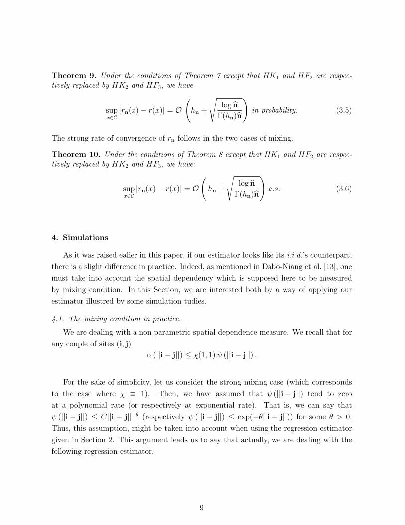
Theorem 9. Under the conditions of Theorem 7 except that HK1 and HF2 are respec-tively replaced by HK2 and HF3, we have

supx∈C

|rn(x) − r(x)| = O

(hn +

√log n

Γ(hn)n

)in probability. (3.5)

The strong rate of convergence of rn follows in the two cases of mixing.

Theorem 10. Under the conditions of Theorem 8 except that HK1 and HF2 are respec-tively replaced by HK2 and HF3, we have:

supx∈C

|rn(x) − r(x)| = O

(hn +

√log n

Γ(hn)n

)a.s. (3.6)

4. Simulations

As it was raised ealier in this paper, if our estimator looks like its i.i.d.’s counterpart,

there is a slight difference in practice. Indeed, as mentioned in Dabo-Niang et al. [13], one

must take into account the spatial dependency which is supposed here to be measured

by mixing condition. In this Section, we are interested both by a way of applying our

estimator illustred by some simulation tudies.

4.1. The mixing condition in practice.

We are dealing with a non parametric spatial dependence measure. We recall that for

any couple of sites (i, j)

α (||i − j||) ≤ χ(1, 1)ψ (||i − j||) .

For the sake of simplicity, let us consider the strong mixing case (which corresponds

to the case where χ ≡ 1). Then, we have assumed that ψ (||i − j||) tend to zero

at a polynomial rate (or respectively at exponential rate). That is, we can say that

ψ (||i − j||) ≤ C||i − j||−θ (respectively ψ (||i − j||) ≤ exp(−θ||i − j||)) for some θ > 0.

Thus, this assumption, might be taken into account when using the regression estimator

given in Section 2. This argument leads us to say that actually, we are dealing with the

following regression estimator.

9

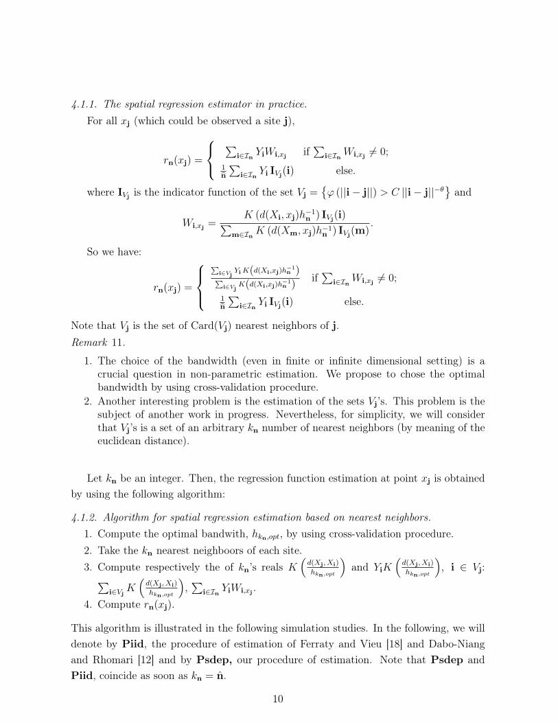
4.1.1. The spatial regression estimator in practice.

For all xj (which could be observed a site j),

rn(xj) =

∑i∈In

YiWi,xjif∑

i∈InWi,xj

6= 0;

1bn

∑i∈In

Yi IVj(i) else.

where IVjis the indicator function of the set Vj =

ϕ (||i − j||) > C ||i − j||−θ

and

Wi,xj=

K (d(Xi, xj)h−1n ) IVj

(i)∑m∈In

K (d(Xm, xj)h−1n ) IVj

(m).

So we have:

rn(xj) =

P

i∈VjYi K(d(Xi,xj)h

−1n )

P

i∈VjK(d(Xi,xj)h

−1n )

if∑

i∈InWi,xj

6= 0;

1bn

∑i∈In

Yi IVj(i) else.

Note that Vj is the set of Card(Vj) nearest neighbors of j.

Remark 11.

1. The choice of the bandwidth (even in finite or infinite dimensional setting) is acrucial question in non-parametric estimation. We propose to chose the optimalbandwidth by using cross-validation procedure.

2. Another interesting problem is the estimation of the sets Vj’s. This problem is thesubject of another work in progress. Nevertheless, for simplicity, we will considerthat Vj’s is a set of an arbitrary kn number of nearest neighbors (by meaning of theeuclidean distance).

Let kn be an integer. Then, the regression function estimation at point xj is obtained

by using the following algorithm:

4.1.2. Algorithm for spatial regression estimation based on nearest neighbors.

1. Compute the optimal bandwith, hkn,opt, by using cross-validation procedure.

2. Take the kn nearest neighboors of each site.

3. Compute respectively the of kn’s reals K(

d(Xj, Xi)

hkn,opt

)and YiK

(d(Xj, Xi)

hkn,opt

), i ∈ Vj:

∑i∈Vj

K(

d(Xj, Xi)

hkn,opt

),∑

i∈InYiWi,xj

.

4. Compute rn(xj).

This algorithm is illustrated in the following simulation studies. In the following, we will

denote by Piid, the procedure of estimation of Ferraty and Vieu [18] and Dabo-Niang

and Rhomari [12] and by Psdep, our procedure of estimation. Note that Psdep and

Piid, coincide as soon as kn = n.

10

4.2. Simulations studies

In order to illustrate our results, we have done some simulations based on observations

(Xi,j, Yi,j), 0 ≤ i, j ≤ 25 such that ∀ i, j, :

Xi,j(t) = Ai,j ∗ (t− 0.5)2 +Bi,j

and

Yi,j = 4A2i,j + εi,j, (4.1)

where A = (Ai, j), B = (Bi, j) and ε = (εi,j) are random variables which will be

specified later on. Note that here we have r(X) = 4.X ′′ (where f ′′ denotes the second

derivatives of a funtion f )). We are first (on Section 1.2.1.) interesting with the estimation

of Model (4.1) based on i.i.d. observations Zi = (Xi, Yi) (the sequences A, B and ε are

then i.i.d. random variables); after that we deal on Section 1.2.2, with Model (4.1)

generated with the spatial dependence structure.

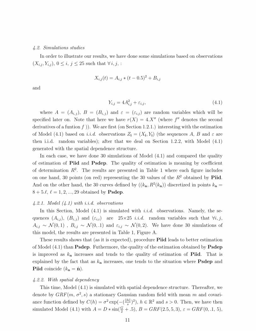
In each case, we have done 30 simulations of Model (4.1) and compared the quality

of estimation of Piid and Psdep. The quality of estimation is meaning by coefficient

of determination R2. The results are presented in Table 1 where each figure includes

on one hand, 30 points (on red) representing the 30 values of the R2 obtained by Piid.

And on the other hand, the 30 curves defined by ((kn, R2(kn)) discretized in points kn =

8 + 5.ℓ, ℓ = 1, 2, ..., 29 obtained by Psdep.

4.2.1. Model (4.1) with i.i.d. observations

In this Section, Model (4.1) is simulated with i.i.d. observations. Namely, the se-

quences (Ai,j), (Bi, j) and (εi,i) are 25×25 i.i.d. random variables such that ∀i, j,

Ai,j ∼ N (0, 1) , Bi,j ∼ N (0, .1) and εi,j ∼ N (0, 2). We have done 30 simulations of

this model, the results are presented in Table 1, Figure A.

These results shows that (as it is expected), procedure Piid leads to better estimation

of Model (4.1) than Psdep. Futhermore, the quality of the estimation obtained by Psdep

is improved as kn increases and tends to the quality of estimation of Piid. That is

explained by the fact that as kn increases, one tends to the situation where Psdep and

Piid coincide (kn = n).

4.2.2. With spatial dependency

This time, Model (4.1) is simulated with spatial dependence structure. Thereafter, we

denote by GRF (m, σ2, s) a stationary Gaussian random field with mean m and covari-

ance function defined by C(h) = σ2 exp(−(‖h‖s

)2), h ∈ R2 and s > 0. Then, we have then

simulated Model (4.1) with A = D ∗ sin(G2

+ .5), B = GRF (2.5, 5, 3), ε = GRF (0, .1, 5),

11

20 40 60 80 100 120 140

0.0

0.2

0.4

0.6

0.8

1.0

Number of neighbourbs

Coeffic

ient of dete

rmin

ation

********

**

*****************

***

20 40 60 80 100 120 140

0.0

0.2

0.4

0.6

0.8

1.0

Number of neighbourbs

Co

eff

icie

nt

of

de

term

ina

tio

n

************

****

*

********

*****

A. With i.i.d. observations B. With spatial dependency, with a=50

20 40 60 80 100 120 140

0.0

0.2

0.4

0.6

0.8

1.0

Number of neighbourbs

Coeffic

ient of dete

rmin

ation

**

**

*

***

*

*

**

**

*

**

***

*

*

*

**

*

*

***

20 40 60 80 100 120 140

0.0

0.2

0.4

0.6

0.8

1.0

Number of neighbourbs

Coeffic

ient of dete

rmin

ation

*

****************

*

***

********

*

C. With spatial dependency,with a=20 D. With spatial dependency,with a=5

Table 1: Values of the coefficient of determination R2

12

0 5 10 15 20 25

01

23

45

h

valu

es o

f C

(h)

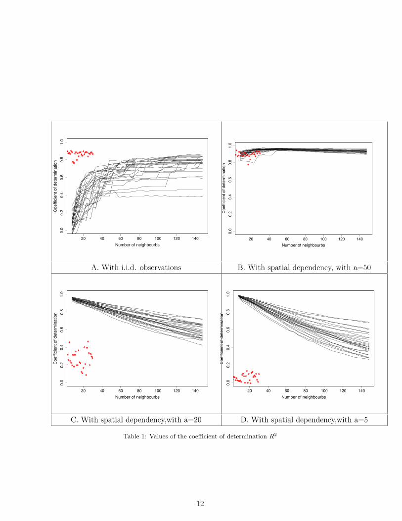
Figure 4.1: Covariance function with σ2= 5 and s = 5

G = GRF (0, 5, 3) and Di = 1n

∑j exp

(−‖i−j‖

a

)

(D(i,j) = 125×25

∑1≤m,t≤25 exp

(−‖(i,j)−(m,t)‖

a

)). The function D is here to ensure and con-

trol the spatial mixing condition (even if using the Gaussian Random Fields also brings

some spatial dependency). Indeed, our model can be seen verifying a mixing condition

with ψ (h) → 0 at exponential rate. Then, the greater is a, the weaker is the spatial

dependency. Futhermore, if a→ ∞ , Di → 1.

Now, let us respectively consider cases a = 50, 20, 5. The case a = 50 corresponds to

the one we discuss just before since Di ≃ 1. The results are presented on Table 1-Figure B

where, whatever the values of kn, one has a good quality of estimation both with Psdep

and Piid and the values are almost equal. The fact that quality of estimation by Piid

is as good (despite the existence of dependence) is explained by the high valued of a

and the number of independent observations is then not negligeable. Actually, this later

case corresponds to A ≃ sin(G2

+ .5) and Model (4.1) is based both on spatial dependent

observations and nearly i.i.d. observations. In fact, since (in these conditions) Model

(4.1) is based on Gaussian random fields with covariance function C and scale s ≤ 5 (see

13

0 20 40 60 80 100

0.6

00.6

50.7

00

.75

0.8

00

.85

0.9

00

.95

kn

valu

es o

f R

^2

Figure 4.2: kn versus R2 with a = 20

Figure 4.1), observations of sites i and j with ‖i − j‖ < 15 are spatial dependent and

nearly independent from ‖i − j‖ ≥ 15. So, our observations are a mixture of i.i.d. and

dependent observations. Thus, to move away from independence, it suffises to lower the

value of a. That is done in the context of Table1, figures C and D respectively with a = 20

and a = 5. One can see that the quality of estimation of Piid deteriorate as a decreases

and is very bad with a = 5.

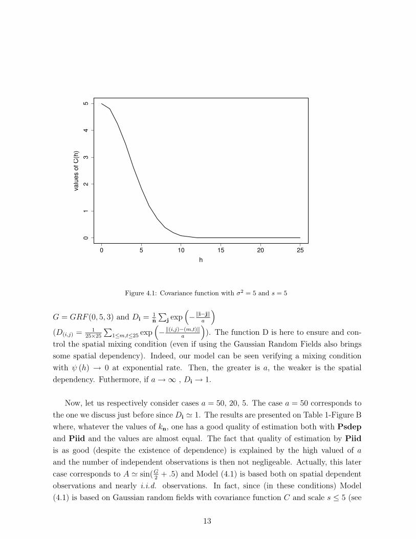
Other interesting results are the evolution of quality estimation of Psdep in Table 1,

figures B, C and D which are different from Figure 4.1.A. In fact, as one can see on Figure

4.2 there is an optimal kn around which the quality of estimation is better and quality is

increasingly bad when away from this values and tends to that of Piid. These results are

not visible in the previous figures the discretization is to coarse.

14

0 5 10 15 20 25

05

10

15

20

25

0 5 10 15 20 25

05

10

15

20

25

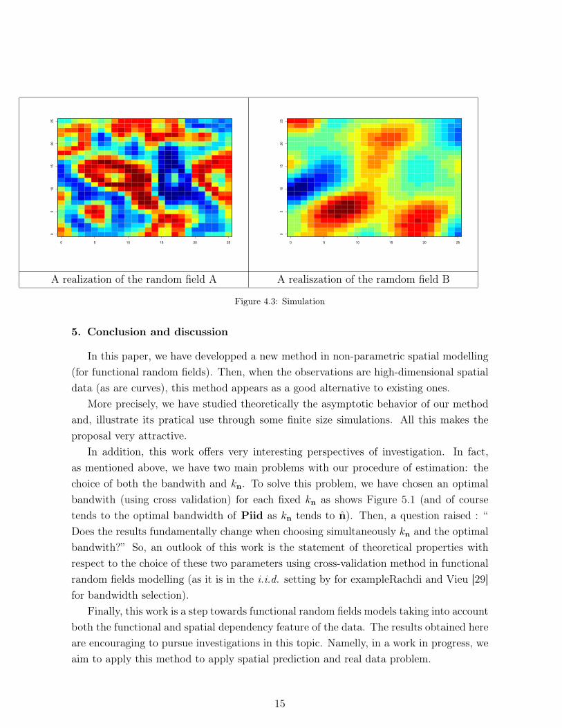
A realization of the random field A A realiszation of the ramdom field B

Figure 4.3: Simulation

5. Conclusion and discussion

In this paper, we have developped a new method in non-parametric spatial modelling

(for functional random fields). Then, when the observations are high-dimensional spatial

data (as are curves), this method appears as a good alternative to existing ones.

More precisely, we have studied theoretically the asymptotic behavior of our method

and, illustrate its pratical use through some finite size simulations. All this makes the

proposal very attractive.

In addition, this work offers very interesting perspectives of investigation. In fact,

as mentioned above, we have two main problems with our procedure of estimation: the

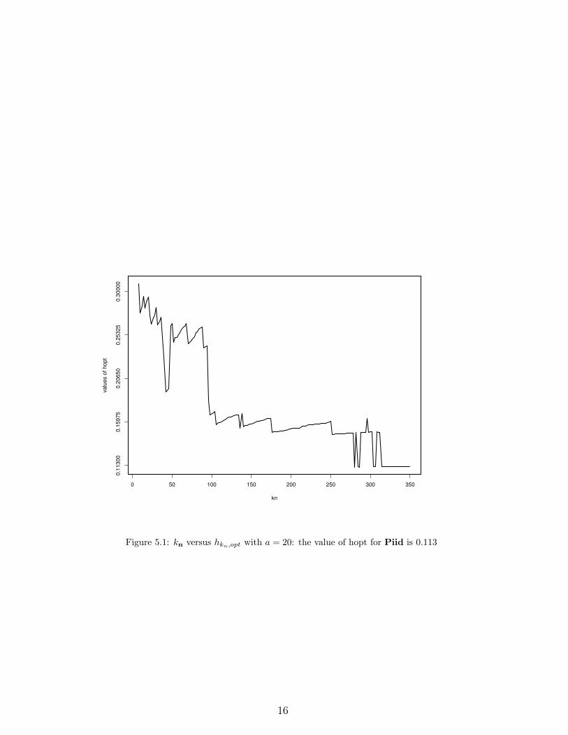
choice of both the bandwith and kn. To solve this problem, we have chosen an optimal

bandwith (using cross validation) for each fixed kn as shows Figure 5.1 (and of course

tends to the optimal bandwidth of Piid as kn tends to n). Then, a question raised : “

Does the results fundamentally change when choosing simultaneously kn and the optimal

bandwith?” So, an outlook of this work is the statement of theoretical properties with

respect to the choice of these two parameters using cross-validation method in functional

random fields modelling (as it is in the i.i.d. setting by for exampleRachdi and Vieu [29]

for bandwidth selection).

Finally, this work is a step towards functional random fields models taking into account

both the functional and spatial dependency feature of the data. The results obtained here

are encouraging to pursue investigations in this topic. Namelly, in a work in progress, we

aim to apply this method to apply spatial prediction and real data problem.

15

0 50 100 150 200 250 300 350

0.1

1300

0.1

5975

0.2

0650

0.2

5325

0.3

0000

kn

valu

es o

f hopt

Figure 5.1: kn versus hkn,opt with a = 20: the value of hopt for Piid is 0.113

16

6. Appendix

This section is devoted to prove the consistency result stated in the previous sections.

For that, we recall three lemmas which can be find to Carbon et al. [5] which will be used

in the following. As previously, along this section we will denote by C a positive generic

constant.

Lemma 12. Suppose E1, ..., Er be sets containing m sites each with dist(Ei, Ej) ≥ γ forall i 6= j where 1 ≤ i ≤ r and 1 ≤ j ≤ r. Suppose Z1, ..., Zr is a sequence of real-valuedr.v.’s measurable with respect to B(E1), ...,B(Er) respectively, and Zi takes values in [a, b].Then there exists a sequence of independent r.v.’s Z∗

1 , ..., Z∗r independent of Z1, ..., Zr such

that Z∗i has the same distribution as Zi and satisfies

r∑

i=1

E|Zi − Z∗i | ≤ 2r(b− a)χ((r − 1)m,m)ψ(γ) (6.1)

Lemma 13.

(i) Suppose that (2.2) holds. Denote by Lr(F) the class of F−measurable r.v.’s X sat-isfying ‖X‖r = (E|X|r)1/r < ∞. Suppose X ∈ Lr(B(E)) and X ∈ Lr(B(E ′)). Assumealso that 1 ≤ r, s, t <∞ and r−1 + s−1 + t−1 = 1. Then

|EXY − EXEY | ≤ C‖X‖r‖Y ‖sχ(Card(E), Card(E ′))ψ(dist(E,E ′))1/t. (6.2)

(ii) For r.v.’s bounded with probability 1, the right-hand side of (6.2) can be replaced by

Cχ(Card(E), Card(E ′))ψ(dist(E,E ′)).

Lemma 14.

If (2.5) holds for θ > 2N , then

∞∑

i=1

iN−1(ψ(i))a <∞ (6.3)

for some 0 < a < 1/2.

6.1. Proofs of the results for the local convergence case.

Proof. of Lemma 3: Let

Zi, x =Ki

∆x

K(d (Xi, x)h

−1n

)− E

(Ki

∆x

K(d (Xi, x)h

−1n

)), Sn =

∑

i∈In

Zi, x,

17

where ∆x = E (K (d (X, x)h−1n )), Ki = 1 (for the case of fn) or Ki = Yi (for the case of

ϕn).

We have var(Gn(x)) = var(Sn/n), then

var(Gn(x)) ≤ n−2

(∑

i∈In

E(Z2i,x) +

∑

i∈In

∑

j∈In, ik 6=jk for some k

|E(Zi,xZj,x)|

).

Let us first consider the case whereKi = 1 and set J1,x,n = (npxhn

)(n−2

∑i∈In

E(Z2i,x)).

Then, we have the inequality

J1,x,n ≤px

hn

(∆x)2

[E(K2

(d (X, x)h−1

n

))]

which leads by assumption HK1 to:

J1,x,n ≤ Cpx

hn

∆x

E (K (d (X, x)h−1n ))

∆x

= Cpx

hn

∆x

.

Furthermore, it is easy to see that 0 < C ≤ pxhn/∆x ≤ C ′ (see for example Lemma 4.3

or 4.4 of Ferraty and Vieu [18]) where C and C ′ are two real constants, so:

limn→∞

J1,x,n <∞.

To continue the proof, we set:

J2,x,n =(npx

hn))n−2

∑ ∑

0<dist(i,j)≤mn

E(Zi,xZj,x) +∑ ∑

dist(i,j)>mn

E(Zi,xZj,x)

= J1

2,x,n+J22,x,n.

where mn is a positive real (depending on n).

Now, since

E(Zi,xZj,x) ≤C

(∆x)2|P ((Xi, Xj) ∈ B(x, hn) ×B(x, hn))| ,

by assumptions HK1, where 0 < ǫ1 < 1 one get:

E(Zi,xZj,x) ≤C

(∆x)2(px

hn)1+ǫ1 ≤ C(px

hn)ǫ1−1

and by the way the inequality:

J12,x,n ≤ C(npx

hn)nmN

n n−2(pxhn

)ǫ1−1 = CmNn p

xhn

ǫ1 .

Setting mn = pxhn

−(1−γ)ǫ1/ν , where ν = −N − ǫ1 + (1 − γ)ǫ1Na−1 with γ and ǫ1 some

small positive numbers such that a−1ǫ1 − (N + ǫ1)(N(1− γ))−1 > 1 (this is possible since

0 < a < 1/2), we get:

J12,x,n ≤ C(px

hn)1−N(1−γ)/ν ,

18

thus limn→∞ J12,x,n = 0 since ν > N(1 − γ).

Let us turn to J22,x,n and let γ′ = 1−(1−γ)ǫ1, δ = 2(1−γ′)/γ′. Notice that γ′ = 2/(2+δ)

and 1−γ′ = δ/(2+δ). We apply Lemma 2.1 of Tran [33]with r = s = 2+δ; h = (2+δ)/δ

and get the inequality:

|E (Zi,xZj,x)| ≤ C

(1

(∆x)2+δE2+δ

[K(d (Xk, x)h

−1n

)])γ′

(ψ(‖i − j‖))1−γ′

;

which leads to:

J22,x,n ≤ (n−1px

hn)∑ ∑

‖i−j‖>mn

C

(1

(∆x)2+δE2+δ

[K(d (Xk, x)h

−1n

)])γ′

(ψ(‖i − j‖))1−γ′

.

≤ C(n−1pxhn

)(pxhn

)−γ′(1+δ)∑ ∑

‖i−j‖>mn

(ψ(‖i − j‖))1−γ′

≤ C(n−1pxhn

)(pxhn

)−γ′(1+δ)n∑

‖i‖>mn

(ψ(‖i‖))1−γ′

≤ C(pxhn

)−1+γ′∑

‖i‖>mn

(ϕ(‖i‖))1−γ′

.

It comes from assumption∑∞

i=1 iN−1(ψ(i))a < ∞ that ψ(i) = o(i−N/a) and since ϕ is

a decreasing function we have ϕ(t) = o(t−N/a) as t→ ∞ and

‖i‖ν (ψ(‖i‖))1−γ′

= ‖i‖νo(‖i‖−N(1−γ′)/a) = o(‖i‖−N−ǫ1),

because ν = −N − ǫ1 + (1 − γ)ǫ1Na−1 > 0. Then,

∑

i∈In

‖i‖ν (ψ(‖i‖))1−γ′

<∞.

Furthermore (pxhn

)1−γ′

m−νn = 1 so:

lim sup J22,x,n ≤ C lim sup (px

hn)−1+γ′

∑

‖i‖>mn

(ψ(‖i‖))1−γ′

≤ C lim sup(pxhn

)−1+γ′

m−νn

∑

‖i‖>mn

‖i‖ν (ψ(‖i‖))1−γ′

≤ C lim sup∑

‖i‖>mn

‖i‖ν (ψ(‖i‖))1−γ′

.

This last term tends to zero as mn tends to infinity. For the case Ki = Yi the proof is the

same as the previous one since Y is bounded. This yields the proof.

19

Proof. of Theorem 4.

We consider the decomposition:

rn(x)−r(x) =1

fn(x)ϕn(x) − E(ϕn(x)) − (r(x) − E(ϕn(x)))−

r(x)

fn(x)fn(x) − 1 , x ∈ E .

(6.4)

Let:

I1(x) = ϕn(x) − E(ϕn(x)),

I2(x) = r(x) − E(ϕn(x)).

and

I3(x) = fn(x) − 1.

Then, we have for a given k ∈ NN

I2(x) = r(x) − E

(Y

∆x

K(d (X, x)h−1

n

))= r(x) − E

(E

(Yk

∆x

K(d (Xk, x)h

−1n

)|Xk

))

= r(x) − E

(r(Xk)

(K (d (Xk, x)h

−1n )

∆x

))

= E

((r(x) − r(Xk))

(K (d (Xk, x)h

−1n )

∆x

)).

Since the support of the function K is [0, 1], we have:

r(x) − r(Xk) ≤ supu∈B(x,hn)

|r(x) − r(u)|.

So, I2(x) ≤ supu∈B(x,hn) |r(x) − r(u)| converges to zero by the continuity assumption of r

at x.

We now focus on the convergence of I1(x). Note that the proof of I3(x) is derive from

the one of I1(x) by setting Yi = 1.

Let :

Qn(x) = ϕn (x) − E (ϕn (x)) =∑

i∈In

Zi,n, x − E (Zi,n) =∑

i∈In

Z ′i,n, x, x ∈ E ,

where

Zi,n, x =Yi∆i

n, ∆i =

K (d (Xi, x)h−1n )

EK (d (X, x)h−1n )

20

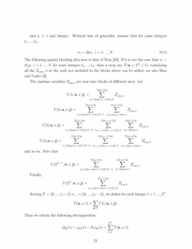
and p ≥ 1 and integer. Without loss of generality assume that for some integers

t1, ..., tN ,

ni = 2pti, i = 1, ..., N. (6.5)

The following spatial blocking idea here is that of Tran [33]. If it is not the case that ni =

2tip, i = 1, ..., N for some integers t1, ..., tN , then a term say T (n, x, 2N + 1), containing

all the Zi,n, x’s at the ends not included in the blocks above can be added, see also Biau

and Cadre [3].

The random variables Z ′i,n, x are now into blocks of different sizes. Let

U(1,n, x, j) =

(2jk+1)p∑

ik=2jkp+1, 1≤k≤N

Z ′i,n, x,

U(2,n, x, j) =

(2jk+1)p∑

ik=2jkp+1, 1≤k≤N−1

2(jN+1)p∑

iN=(2jN+1)p+1

Z ′i,n, x,

U(3,n, x, j) =

(2jk+1)p∑

ik=2jkp+1, 1≤k≤N−2

2(jN−1+1)p∑

iN−1=(2jN−1+1)p+1

(2jN+1)p∑

iN=2jNp+1

Z ′i,n, x,

U(4,n, x, j) =

(2jk+1)p∑

ik=2jkp+1, 1≤k≤N−2

2(jN−1+1)p∑

iN−1=(2jN−1+1)p+1

2(jN+1)p∑

iN=(2jN+1)p+1

Z ′i,n, x,

and so on. Note that

U(2N−1,n, x, j) =

2(jk+1)p∑

ik=(2jk+1)p+1, 1≤k≤N−1

(2jN+1)p∑

iN=2jNp+1

Z ′i,n, x.

Finally,

U(2N ,n, x, j) =

2(jk+1)p∑

ik=(2jk+1)p+1, 1≤k≤N

Z ′i,n, x.

Setting T = 0, ..., t1 −1× ...×0, ..., tN −1, we define for each integer l = 1, ..., 2N ,

T (n, x, l) =∑

j∈T

U(l,n, x, j).

Then we obtain the following decomposition

Qn(x) = ϕn(x) − Eϕn(x) =2N∑

l=1

T (n, x, l).

21

To prove that Qn(x) = O(√

log bn

bnpxhn

)in probability or a.s., it is sufficient to show that

T (n, x, l) = O

(√log n

npxhn

)a.s. or in probability (6.6)

for each l = 1, ..., N . Without loss of generality we will show (6.6) for l = 1.

Let us prove that given an arbitrary large positive constant c, there exists a positive

constant C such that for any η > 0

P

[|T (n, x, 1)| > η

√log n

npxhn

]≤ C(n−c + β1bn)

where β1bn = χ(n, pN)ϕ(p)ǫ−1n .

Let

T (n, x, 1) =∑

j∈T

U(1,n, x, j).

be the sum of

t = t1 × ...× tN (6.7)

of the U(1,n, x, j)’s. Note that U(1,n, x, j) is measurable with respect to the σ−field

generated by Xi with i belonging to the set of sites

Ii, j = i : 2jkp+ 1 ≤ ik ≤ (2jk + 1)p, k = 1, ..., N

These sets of sites are separated by a distance greater than p. Enumerate the random

variables’s U(1,n, x, j) and the corresponding σ−field with which they are measurable in

an arbitrary manner and refer to them respectively as V1, ..., Vbt and B1, ...,Bbt. By Lemma

6.1 of Carbon et al (1997), we approximate V1, ..., Vbt by V ∗1 , ..., V

∗bt. We have

|Vi| = |U(1,n, x, j)| < CpN n−1. (6.8)

Let ǫn = η√

log bn

bnpxhn

where η > 0 is a constant to be chosen later.

Since we have T (n, x, 1) =∑

bt

i=1 Vi, then

P [|T (n, x, 1)| > ǫn] ≤ P

∣∣∣∣∣∣

bt∑

i=1

V ∗i

∣∣∣∣∣∣> ǫn/2

+ P

bt∑

i=1

|Vi − V ∗i | > ǫn/2

. (6.9)

By Markov’s inequality and using (6.8), (6.1) and recall that the sets of sites with respect

to which Vi’s are measurable are separated by a distance greater than p, we get

22

P

bt∑

i=1

|Vi − V ∗i | > ǫn

≤ C tpN n−1χ(n, pN)ψ(p)ǫ−1

n ∼ β1bn. (6.10)

Let

λn =(npx

hnlog n

)1/2, (6.11)

p =

[(npx

hn

4λn

)1/N]∼

(npx

hn

log n

)1/2N

. (6.12)

It is clear that, λnǫn = η log n.

If (2.5) holds for θ > 2N , we have (by Lemma 3)

limn→∞

npxhn

(Rn(x) + Un(x)) < C (6.13)

where C is a positive constant and

Un(x) =∑

i∈In

E(Zi,n,x)2

Rn(x) =∑

i∈In

∑

l∈In, ik 6=lk for some k

|Cov(Zi,n,x, Zl,n,x)|.

By (6.3) and (6.13), we have

λ2n

bt∑

i=1

E(V ∗i )2 ≤ Cnpx

hn(Un(x) +Rn(x)) log n < C log n.

Using (6.8), we get |λnV∗i | < 1/2 for large n. We deduce from Berstein’s inequality

that

P

∣∣∣∣∣∣

bt∑

i=1

V ∗i

∣∣∣∣∣∣> ǫn

≤ 2 exp(−λnǫn + λ2

n

bt∑

i=1

E(V ∗i )2) ≤ 2 exp((−η + C) log n) ≤ n−c

(6.14)

for sufficiently large n. We deduce from (6.9), (6.10) and (6.14) that

P [|T (n, x, 1)| > ǫn] ≤ C(n−c + β1bn)

To complete the proof, we will show that β1bn → 0. Recall that

β1bn = χ(n, pN)ψ(p)ǫ−1n . (6.15)

23

Furthermore, condition (2.3) allows to show that θ > 2N is equivalent to (β1bn)−1 → ∞.

Actually, we have

β1bn ≤ Cχ(n, pN)p−θǫ−1n

≤ C

(npx

hn

log n

)(1/2)−(θ/2N) ((npx

hn/ log n)

) 12

= C

(npx

hn

log n

)−θ+2N2N

Analogously to the condition (2.3), we have under (2.4):

β1bn ≤ Cψ(n, pN)p−θǫ−1n

≤ Cneβ

(npx

hn

log n

)(1/2)−(θ/2N)

= C(n(px

hn/ log n)θ1

)−θ+N(2eβ+1)2N .

Then, condition(n(px

hn/ log n)θ1

)→ ∞ leads to β1bn → 0.

Proof. of Theorem 5

Under (2.3), we get (see the proof of Theorem 4):

β1bn ≤ C

(npx

hn

log n

)−θ+2N2N

,

then

β1bnng(n) ≤

(n

(px

hn

log n

)θ∗1

g(n)2N

4N−θ

) 4N−θ2N

.

Analogously to (2.3), we have under (2.4):

β1bnng(n) ≤

(n

(px

hn

log n

)θ∗2

g(n)2N

N(2eβ+3)−θ

)N(2eβ+3)−θ

2N

Then the assumption

(n(

pxhn

log bn

)θ∗1g(n)

2N4N−θ

) 4N−θ2N

→ ∞ or

(n(

pxhn

log bn

)θ∗2g(n)

2N

N(2eβ+3)−θ

)N(2eβ+3)−θ

2N

→

∞ implies that β1bnng(n) → 0, this last yields that∑

n∈NN β1bn <∞ and the proof is com-

plete by Borel-Cantelli’s Lemma.

24

6.2. Proofs of results of uniform convergence case.

Proof. of Lemma 6: It is similar to that of Lemma 3, it suffices to replace pxhn

by

Γ(hn).

To show theorems 7-10, we consider the fact that the set C is covered by dn balls

Bk = B(xk, ρn) of radius ρn and center at xk and we define:

S1n = max1≤k≤dn

supx∈Bk

|ϕn(x) − ϕn(xk)|,

S2n = max1≤k≤dn

supx∈Bk

|Eϕn(xk) − Eϕn(x)|,

S3n = max1≤k≤dn

|ϕn(xk) − Eϕn(xk)|.

Then,

supx∈C

|ϕn(x) − Eϕn(x)| ≤ S1n + S2n + S3n.

It easy to see that under H2 and HK2, S1n and S2n are equal to o(√

log bn

Γ(hn)bn

)in probability

(or almost surely).

It remains to show that S3n = O(√

log bn

Γ(hn)bn

)in probability (resp. almost surely)

which is equivalent to show that max1≤j≤dn|T (n, xj, 1)| = O

(√log bn

Γ(hn)bn

)probability (resp.

almost surely).

Proof. of Theorem 7

We have:

P [supx∈C

|T (n, x, 1)| > ǫn] ≤ Cdn(n−c + β1bn),

where pxhn

is replaced by Γ(hn) in the expressions of ǫn and β1bn of the previous proof.

To complete the proof, we will show that dnn−c → 0 and dnβ1bn → 0. We have

dnn−c ≤ Cnβ−c

which goes to zero if c > β. We get the following inequality, under (2.3):

dnβ1bn ≤ Cnβ

(nΓ(hn)

log n

)−θ+2N2N

=(n(Γ(hn)/ log n)θ2

)−θ+2N(β+1)2N . (6.16)

25

Analogously to (2.3), we have under (2.4):

dnβ1bn ≤ Cnβneβ

(nΓ(hn)

log n

)(1/2)−(θ/2N)

=(n(Γ(hn)/ log n)θ3

)−θ+N(2β+2eβ+1)2N . (6.17)

This yields the proof.

Proof. of Theorem 8

We have under (2.3):

dnβ1bn ≤ Cnβ

(nΓ(hn)

log n

)−θ+2N2N

,

Then,

dnβ1bnng(n) ≤ C

(n

(Γ(hn)

log n

)θ∗3

g(n)2N

N(2β+4)−θ

)N(2β+4)−θ

2N

.

In the case where (2.4) is satisfied, we get:

dnβ1bnng(n) ≤ C

(n

(Γ(hn)

log n

)θ∗4

g(n)2N

N(2β+2eβ+3)−θ

)N(2β+2eβ+3)−θ

2N

.

Then, condition(n(Γ(hn)/ log n)θ∗3 (g(n))

2N−θ+2N(β+2)

)→ ∞ or

(n(Γ(hn)/ log n)θ∗4 (g(n))

2N

−θ+N(2β+2eβ+3)

)→ ∞ is equivalent to ng(n)β1bn → 0 which implies∑

n∈NN β1bn <∞, then the theorem follows by Borel-Cantelli Lemma.

Proof. of Theorem 9

According to Theorem 7, we have:

supx∈C

|ϕn(x) − E(ϕn(x))| = O

(√log n

Γ(hn)n

), in probability.

and

supx∈C

|fn(x) − 1| = O

(√log n

Γ(hn)n

), in probability.

26

We get also by HF3 (see the proof of Theorem 4):

supx∈C

|r(x) − E(ϕn(x))| ≤ supx∈C

supu∈B(x,hn)

|r(x) − r(u)| = O (hn) .

Proof. of Theorem 10

According to Theorem 8 and HF3, we have:

supx∈C

|ϕn(x) − E(ϕn(x))| = supx∈C

|fn(x) − 1| = O

(√log n

Γ(hn)n

), a.s

and

supx∈C

|r(x) − E(ϕn(x))| ≤ supx∈C

supu∈B(x,hn)

|r(x) − r(u)| = O (hn) .

The proof is therefore complete.

References

[1] Anselin, L., Florax, R. J. M., 1995. New Directions in Spatial Econometrics. Springer,

Berlin.

[2] Besse, P., Cardot, H., Stephenson, D., 2000. Autoregressive forecasting of some func-

tional climatic variations. Scand. J. Statist. 27, 673–687.

[3] Biau, G., Cadre, B., 2004. Nonparametric spatial prediction. Stat. Inference Stoch.

Process. 7, 327–349.

[4] Bosq, D., 2000. Linear Processes in Function Spaces: Theory and applications. Lec-

ture Notes in Statistics, Springer-Verlag, New York.

[5] Carbon, M., Francq, C., Tran, L. T., 2007. Kernel regression estimation for random

fields. J. Statist. Plann. Inference 137 (Issue 3), 778–798.

[6] Carbon, M., Hallin, M., Tran, L. T., 1996. Kernel density estimation for random

fields. Stat. Proba. Lett. 36, 115–125.

[7] Carbon, M., Tran, L. T., Wu, B., 1997. Kernel density estimation for random fields:

The l1 theory. J. Nonparametr. Stat. 6, 157–170.

[8] Cardot, H., Johannes, J., 2010. Thresholding projection estimators in functional

linear models. J. Multivariate Anal. 101, 395–408.

27

[9] Chilès, J., P., D., 1999. Geostatistics. Modeling spatial uncertainty. Wiley Series in

Probability and Mathematical Statistics, New-York.

[10] Cressie, N. A., 1991. Statistics for Spatial Data. Wiley Series in Probability and

Mathematical Statistics, New-York.

[11] Dabo-Niang, S., Ferraty, F., 2008. Functional and Operatorial Statistics. Springer-

Verlag, New-York.

[12] Dabo-Niang, S., Rhomari, N., 2009. Kernel regression estimate in a banach space. J.

Statist. Plann. Inf. 139, 1421–1434.

[13] Dabo-Niang, S., Yao, A., Pischedda, L., Cuny, P., Gilbert, F., 2009. Spatial kernel

mode estimation for functional random, with application to bioturbation problem.

Stochastic Environmental Research and Risk Assessment 24 (4), 487–497.

[14] Dabo-Niang, S., Yao, A. F., 2007. Kernel regression estimation for continuous spatial

processes. Math. Method. Stat. 16 (4), 1–20.

[15] Delicado, P., Giraldo, R., Mateu, J., 2008, pp 135-141. Point-wise kriging for spatail

prediction of functional data. Springer Verlag, Functional and Operatorial Statistics,

edited by S. Dabo-Niang and F. Ferraty.

[16] Doukhan, P., 1994. Mixing - Properties and Examples. Lecture Notes in Statistics,

Springer-Verlag, New York.

[17] Fernandez de Castro, B., Guillas, S., W., G. M., 2005. Technometrics 47 (2), 212–222.

[18] Ferraty, F., Vieu, P., 2006. Nonparametric Functional Data Analysis. Springer-

Verlag, berlin.

[19] Ferré, L., Yao, A., 2005. Smoothed functional inverse regression. Statist. Sinica 15 (3),

665–683.

[20] Guyon, X., 1995. Random Fields on a Network - Modeling, Statistics, and Applica-

tions. Springer, New-York.

[21] Hallin, M., L. Z., Yu, K., 2009. Local linear spatial quantile regression. Bernoulli 15,

659–686.

[22] Hallin, M., Lu, Z., Tran, L. T., 2004. Local linear spatial regression. Ann. Statist.

32 (6), 2469–2500.

28

[23] Lakasaci, A., Fouzia, M., 2009. Nonparametric estimation of conditional quantiles

for functional and spatial dependent variables. C. R. Acad. Sci. Paris Ser. I Math

347 (17-18), 1075–1080.

[24] Li, J., Tran, L., 2008. Nonparametric estimation of conditional expectation. Statist.

Plann. Inference 139, 164–175.

[25] Lu, Z., Chen, X., 2002. Spatial nonparametric regression estimation: Non-isotropic

case. Acta Math. Appl. Sin. Engl. Ser. 18 (4), 641–656.

[26] Lu, Z., Chen, X., 2004. Spatial kernel regression estimation: Weak concistency. Stat.

Proba. Lett 68, 125–136.

[27] Nadaraya, E., 1964. On estimating regression. Theor.Prob.Appl., 141–142.

[28] Nerini, D., Monestiez, P., Manté, C., 2010. A cokriging method for spatial functional.

Journal of Multivariate Analysis 101 (2), 409–418.

[29] Rachdi, M., Vieu, P., 2007. Nonparametric regression for functional data: automatic

smoothing parametrer selection. Statist. Plann. Inference 137 (9), 2784–2801.

[30] Ramsay, J., Silverman, B., 2002. Applied functional data analysis; Methods and case

studies. Springer-Verlag, New York.

[31] Rio, E., 2000. Théorie Asymptotic des Processus Aléatoires Faiblement Dépendants.

Springer-Verlag, Berlin.

[32] Ripley, B., 1981. Spatial Statistics. Wiley, New-York.

[33] Tran, L. T., 1990. Kernel density estimation on random fields. J. Multivariate Anal.

34, 37–53.

[34] Watson, G., 1964. Smooth regression analysis. Sankhya, Ser. A 26, 359–372.

29